multiple echo diffusion tensor acquisition technique

Magnetic Resonance

Multiple echo diffusion tensor acquisition technique

Eric E. Sigmund4, Yi-Qiao SongSchlumberger-Doll Research, Ridgefield, CT 06877, USA

Received 9 August 2005; accepted 21 October 2005

Abstract

The standard method of diffusion tensor imaging (DTI) involves one diffusion-sensitizing gradient direction per acquired signal. This

paper describes an alternative method in which the entire direction set required for calculating the diffusion tensor is captured in a few scans.

In this method, a series of radiofrequency (RF) pulses are applied, resulting in a train of spin echoes. A pattern of applied magnetic field

gradients between the RF pulses generates a different diffusion weighting in both magnitude and direction for each echo, resulting in a dataset

sufficient to determine the tensor. This significantly reduces the time required for a full DTI scan and potentially allows a tradeoff of this time

for image quality. In the present work, this method is demonstrated in an anisotropic diffusion phantom (asparagus).

D 2006 Elsevier Inc. All rights reserved.

Keywords: DTI; MMME; Multiple echo; Diffusion tensor

1. Introduction

1.1. Standard DTI

Diffusion tensor imaging (DTI) [1,2] is a specific type of

diffusion-weighted MRI that maps out anisotropically

restricted diffusion in three dimensions. In this type of

scan, the diffusion-weighting gradient is typically varied in

both orientation and strength to determine the apparent

diffusion coefficient along many different directions. This

information is then used to determine the diffusion tensor,

which is the 3D generalization of the diffusion coefficient to

anisotropic motion. Mathematically, the diffusion tensor D

is a 3�3 matrix that enters the spin magnetization

attenuation in a quadratic form:

M

M0

¼ exp �Xij

bijDij

! ð1Þ

or written in the form of a set of linear equations,

� ln M=M0ð Þnumn ¼Xij

bij;nDij ð2Þ

where n labels acquisitions corresponding to different

applied gradient directions, and bij,n are the diffusion-

0730-725X/$ – see front matter D 2006 Elsevier Inc. All rights reserved.

doi:10.1016/j.mri.2005.10.015

4 Corresponding author. Tel.: +1 203 431 5561; fax: +1 203 438 3819.

E-mail address: [email protected] (E.E. Sigmund).

weighting factors for each experiment, determined by the

particular radiofrequency (RF) and gradient pulse sequence

[3–5]. The eigenvalues of the diffusion tensor are the

principal diffusivities ki, and the eigenvectors are the

principal orientations ei. These parameters are used to

calculate scalar properties of the tensor such as the fractional

anisotropy (FA) and the average diffusivity or Trace(D),

according to Ref. [1].

FA ¼

ffiffiffiffiffiffiffiffiffiffiffiffiffiffiffiffiffiffiffiffiffiffiffiffiffiffiffiffiffiffiffi3

2

P3i¼1

ðki�hkiÞ2

P3i¼1

k2i

vuuuuuut ð3Þ

TraceðDÞ=3 ¼ hki ¼ k1 þ k2 þ k33

: ð4Þ

The FA and Trace parameters offer complementary scalar

information in that the former quantifies the orientational

anisotropy in the object, while the latter averages over it. Both

are clinically useful in tissue identification and diagnosis.

In order to measure the diffusion tensor elements Dij in

the laboratory frame, at least six linearly independent

vectors b=[bxx, byy, bzz, bxy, byz, bxz] must be generated

and an amplitude collected for each. In each voxel of the

image, these amplitudes are divided by that from another

experiment with no diffusion weighting (b=0). The range of

diffusion weighting is often covered by choosing one

Imaging 24 (2006) 7–18

Fig. 1. MMME diffusion tensor acquisition technique. The four RF pulses applied generate a series of 13 separate echoes, each of which carries different

diffusion weighting in up to three dimensions. Each gradient direction (Gx, Gy, Gz) serves a dual role of imaging resolution (read, phase, slice gradients) and

diffusion weighting.

E.E. Sigmund, Y.-Q. Song / Magnetic Resonance Imaging 24 (2006) 7–188

gradient direction and one weighting magnitude per

acquisition, and executing as many acquisitions as direc-

tions needed. This is true for most DTI modalities employed

today, including the most common echo-planar imaging

(EPI) [7] as well as steady-state free precession [8–10].

There are some notable exceptions employing multiple spin

echoes for multiple diffusion directions [11]. The minimal

direction set is six acquisitions, although most research or

clinical DTI measurements employ many more (12, 20, 100,

etc.) [12–14] for either enhanced SNR of processed images

or the measurement of anatomical structures that are not

describable by the tensor model (Eq. (1)), such as crossing

white matter fibers in the brain [15]. Much research

attention has been devoted to optimizing the set of applied

gradient directions [13,14,16–19]. While the standard EPI

modality is by far the fastest imaging method, it also carries

well-known image artifacts such as blurring, signal dropout,

and ghosting due to either its sensitivity to magnetic

susceptibility contrast or the eddy currents generated by

its rapid gradient switching. Alternative DTI modalities

without these artifacts are thus highly desirable. However, to

make up for the loss of speed compared to EPI, other

innovations are required to shorten the overall scan time.

One candidate is to improve directional efficiency, i.e., the

number of different diffusion directions sampled within one

excitation. Particularly for scans involving many directional

samples, this efficiency is quite important.

Recent work [20,21] has demonstrated the utility of a

new diffusometry modality with potential applications to

both spectroscopy and imaging. In this technique, termed

multiple modulation multiple echo (MMME), diffusion

weightings of multiple magnitudes and directions are

applied and measured within a single scan. For cases where

the directional phase space is a significant contributor to

scan time, this technique provides an improvement in

efficiency. In the present work, we show the first diffusion

tensor images acquired with this pulse sequence, termed

MMME Diffusion Tensor Acquisition Technique (MEDI-

TATE). We also elaborate on the optimization of this

method with regard to minimizing correlated errors between

different elements of the diffusion tensor.

Numerous methods have been previously developed that

successfully use multiple echoes for relaxation, diffusion,

image encoding or contrast, or 2D spectroscopy [11,22–30].

In the diffusion tensor case, previous work has employed

multiple spin echoes from multiple inversion pulses [11]

combined with a cylindrical symmetry approximation to

accelerate the DTI scan. We emphasize that the present

work, as in Ref. [21], focuses upon using the full 13 echoes

of the four-pulse MMME sequence to image multidimen-

sional diffusion. The implementation is described in the next

section, followed by a description of the sequence’s

optimization. Finally, we present experimental results on

an asparagus phantom.

1.2. MEDITATE sequence — basic theory

The principle of the MEDITATE technique is described

as follows and illustrated in Fig. 1. A series of four RF

pulses are rapidly applied in uneven time intervals. This

preparation is similar to others such as BURST [25],

DANTE and DUFIS [27]. This action generates a large

number of independently evolving echo pathways, with

magnitudes determined by the flip angles of the RF pulses

[5,31–33]. Different pathways include differing portions of

longitudinal and transverse evolution. We denote each echo

or coherence pathway q by a series of values �1, 0 or 1,

corresponding to co-rotating, longitudinal and counter-

rotating magnetization periods, respectively. The pathways

giving rise to the 13 echoes in the MMME train are listed in

the first column of Table 1.

Between and after the RF pulses, magnetic field gradient

pulses are applied in different combinations. Each of the

three gradients (Gx, Gy, Gz) plays a dual role of position

encoding (read, phase, slice) and diffusion weighting. Along

Table 1

Coherence pathways and relaxation coefficients for the 13 echoes of the

four-pulse MMME sequence

Echo # { q} c1q c2q c1qV c2qV

0 +00� 12 2 4 0

1 0+0� 10 5 3 2

2 ��+0� 9 7 3 2

3 ++0� 9 8 3 2

4 �+� 0 18 0 6

5 0�+� 1 18 0 6

6 +�+� 0 20 0 6

7 �0+� 3 18 1 6

8 00+� 4 18 1 6

9 +0+� 3 20 1 6

10 �++� 0 24 0 8

11 0++� 1 24 0 8

12 +++� 0 26 0 8

The pathways are described by a sequence of values corresponding to the

magnetization states in the four time intervals between the RF pulses of the

sequence (see Fig. 1).

E.E. Sigmund, Y.-Q. Song / Magnetic Resonance Imaging 24 (2006) 7–18 9

one direction (x), a constant field gradient is applied

between and after the RF pulses. This gradient provides a

gradually increasing diffusion weighting along one direction

to the echo train and also serves as a readout gradient for its

detection. This gradient is deactivated during the RF pulses

to avoid slice selection effects. Along the other two

directions ( y and z), pulsed gradients of duration d are

applied in a pattern that preserves the formation of each

echo in the train. The first two gradient pulses are arbitrary,

but once they are fixed the last four are derived from the

echo formation conditionR TE0

q tð ÞG tð Þdt ¼ 0, where TE is

the echo time, q(t) is the coherence pathway and G(t) is the

gradient waveform. The gradient pulses provide diffusion

weighting along the two remaining directions in an amount

and direction that vary from echo to echo. The diffusion-

weighting factors bij for each echo can be calculated in the

standard way [3,4]:

bij ¼ZTE0

ki tð Þkj tð Þdt ð5Þ

where i=x,y,z and TE is the echo time, and the vector k is

calculated from

*k tð Þ ¼

Zt0

cq tVð Þ*G tVð ÞdtV: ð6Þ

c is the proton gyromagnetic ratio. Thus, the directional

phase space in the MMME diffusion sequence is covered

with a combination of gradient waveforms G and magne-

tization histories q. Only those echo pathways that are

transverse ( q=F1) during the pulsed Gy and Gz gradients

will suffer their diffusion weighting. For example, the

pathway generating Echo 2 is exposed to the first gradient

pulse but not the second, whereas the pathway for Echo 5 is

exposed to both, etc. Each echo will have a different

diffusion weighting bij given by Eqs. (5) and (6). Once the

diffusion weightings are determined and the echo magni-

tudes M measured, the diffusion tensor elements Dij are

calculated exactly as is done in a standard diffusion tensor

experiment, by solving the linear set of equations in Eq. (2).

Since there are 13 echoes in this sequence and only six

independent elements of the diffusion tensor, this problem is

overdetermined. However, flip angle and relaxation effects

must be separated out as follows. The full expression of the

amplitude of the qth echo can be written

Mq ¼ M0 fq að Þexp�� c1q

sT1

� cV1qsVT1

� c2qsT2

� cV2qsVT2

�

� exp

��Xij

bij;qDij

�; ð7Þ

where M0 is the total magnetization, fq(a) is a magnetiza-

tion fraction (0b fq(a)b1) depending on the RF flip angles aand the coherence pathway q [20], {c1q, c2q, c1qV , c2qV } are

relaxation coefficients that depend on the coherence

pathway and are listed in Table 1, T1 and T2 are relaxation

times, bij,q is the diffusion-weighting matrix for echo q and

Dij are the diffusion tensor elements. The nondiffusive

terms in this expression can be separated from the data using

analytical calculations or empirical measurements. For

example, the fractions fq(a) can be calculated for any set

of flip angles a [20]. However, if the RF field is spatially

inhomogeneous, this correction will be imperfect. In this

case, a reference experiment without diffusion weighting is

preferable to divide out the terms fq(a). In this spirit, each

measurement in this work involved the ratio of two MMME

scans with the same excitation pulses a: one including both

the steady gradient Gx and the pulsed gradients Gy and Gz,

and one with the steady gradient only and (in general)

different pulse timing. The ratio of the echo magnitudes for

the two cases thus eliminates the coherence pathway factors

fq(a). The pulse timing must be different between the two

scans to avoid canceling the diffusion weighting along the

constant gradient (x) direction, since the gradient magnitude

was kept constant to produce equal readout fields-of-view

(FOVs). This unequal timing means that relaxation con-

tributions must be incorporated in the analysis. This can be

done through a separate measurement of the relaxation rates

to divide out their contributions. Alternatively, the solution

for the diffusion tensor can be expanded to include the

relaxation times as independent variables, since they enter

the problem linearly (Eq. (7)). In practice, this combined

solution was found to be poorly conditioned since the

T2 weighting and diffusion weighting along the constant

gradient axis have similar trends. The conditioning of the

diffusion tensor calculation will be discussed further in the

next section.

This spectroscopic sequence is converted to a 2D

imaging sequence with an additional phase encoding pulse

(GPE), just after the last RF pulse that encodes transverse

position for all of the detected echoes. Although the above

sequence does not contain any slice selection, it could be

-400

-200

0

200

400

b (s

/mm

2 )

121086420

Echo number

bxx

byy

bxy

-1000

-500

0

500

1000

b (s

/mm

2 )

121086420

Echo number

byy

bzz

byz

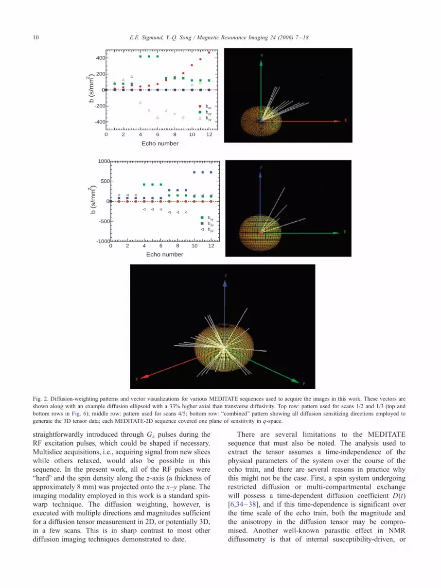
Fig. 2. Diffusion-weighting patterns and vector visualizations for various MEDITATE sequences used to acquire the images in this work. These vectors are

shown along with an example diffusion ellipsoid with a 33% higher axial than transverse diffusivity. Top row: pattern used for scans 1/2 and 1/3 (top and

bottom rows in Fig. 6); middle row: pattern used for scans 4/5; bottom row: bcombined Q pattern showing all diffusion sensitizing directions employed to

generate the 3D tensor data; each MEDITATE-2D sequence covered one plane of sensitivity in q-space.


straightforwardly introduced through Gz pulses during the

RF excitation pulses, which could be shaped if necessary.

Multislice acquisitions, i.e., acquiring signal from new slices

while others relaxed, would also be possible in this

sequence. In the present work, all of the RF pulses were

bhardQ and the spin density along the z-axis (a thickness of

approximately 8 mm) was projected onto the x–y plane. The

imaging modality employed in this work is a standard spin-

warp technique. The diffusion weighting, however, is

executed with multiple directions and magnitudes sufficient

for a diffusion tensor measurement in 2D, or potentially 3D,

in a few scans. This is in sharp contrast to most other

diffusion imaging techniques demonstrated to date.

There are several limitations to the MEDITATE

sequence that must also be noted. The analysis used to

extract the tensor assumes a time-independence of the

physical parameters of the system over the course of the

echo train, and there are several reasons in practice why

this might not be the case. First, a spin system undergoing

restricted diffusion or multi-compartmental exchange

will possess a time-dependent diffusion coefficient D(t)

[6,34–38], and if this time-dependence is significant over

the time scale of the echo train, both the magnitude and

the anisotropy in the diffusion tensor may be compro-

mised. Another well-known parasitic effect in NMR

diffusometry is that of internal susceptibility-driven, or


bbackgroundQ, gradients whose contribution to the spin

dephasing artificially enhances the measured diffusivity. A

variety of pulse sequences have been developed that

compensate for this effect through tailored gradient wave-

forms [39–50], sometimes involving inversions of the

applied gradient that are not duplicated by the internal

gradient. For the MEDITATE sequence, every echo

originates from a different coherence pathway and diffusion

gradient waveform; some are spin-echo pathways, some

stimulated echo pathways, etc. This means that different

echoes will have different susceptibility gradient compen-

sation, which can distort the tensor calculation. Also,

multiple environments, such as intracellular/extracellular

spaces, intra-axonal/extra-axonal spaces, etc., can lead to

multi-exponential relaxation behavior that will confuse the

diffusion information. Finally, unlike the standard EPI

imaging modality, the spin-warp modality employed here

may suffer ghosting artifacts if subject motion occurs

between successive phase encodes. These artifacts would

also vary from echo to echo since each has a different

formation time. All of these effects are each discussed

individually as they apply to the present study in Methods.

1.3. MEDITATE sequence — optimization

Much research attention has been devoted to the

optimization of gradient direction sets for DTI experiments

[12–14,16–19]. Many different direction sets have been

generated and applied; some are motivated by symmetry

arguments, others by minimization of noise propagation and

still others by maximal angular resolution of higher order

structures. Several scalar indices have been proposed to

quantify the quality of one direction set vs. another. While

the MMME sequence affords less flexibility in direction

selection, we will see that it nevertheless compares

favorably with existing DTI direction schemes.

A visual representation of the diffusion weighting of the

MEDITATE-2D sequences used in the present work is

shown in Fig. 2. On the left-hand side of this figure are

shown the numerical values of the coefficient matrix bij for

several scans used in this article. On the right-hand side

are vectors proportional to tvb ¼ffiffiffiffiffiffibxx

p;

ffiffiffiffiffiffibyy

p;

ffiffiffiffiffiffibzz

p� �for

the corresponding patterns at left. The bottom figure

shows the combined direction set for all data contributing

to the 3D tensor measurement described in Results; note

that each of the three MEDITATE-2D sequences contributes

a range of vectors within one plane. This representation

provides a general sense of the angular coverage of a

MEDITATE-2D sequence.

We now proceed to describe the optimization of the

gradient patterns used in the MEDITATE sequence. In the

following discussion, we adopt the following conventional

notation for the processing required to extract the diffusion

tensor. The linear equation set in Eq. (2) can be written in

matrix form:

Bdtd ¼ t

m ð8Þ

where

B ¼

bxx1 byy1 bzz1 2bxy1 2byz1 2bxz1bxx2 byy2 bzz2 2bxy2 2byz2 2bxz2v v v v v v

bxxN byyN bzzN bxyN byzN bxzN

1CCA

0BB@ ð9Þ

is the diffusion-weighting coefficient matrix,

td ¼

Dxx

Dyy

Dzz

Dxy

Dyz

Dxz

1CCCCCCA

0BBBBBB@

ð10Þ

is the diffusion tensor written in vector form, and

tm ¼

� ln M=M0ð Þ1� ln M=M0ð Þ2

v� ln M=M0ð ÞN

1CCA

0BB@ ð11Þ

is the set of measured signals.

We briefly review a quantitative measure of sequence

quality employed for optimization. The goal of this

optimization is the extraction of all the desired elements

Dij, with a minimum of (a) absolute variance and (b)

covariance. In other words, we wish to prepare the

coefficient matrix bij so as to extract each measured value

Dij with the least error and the least confusion with other

tensor elements. An ideal figure of merit for this purpose is

the condition number [13,51,52], which relates the relative

error in the input data to that in the output parameters:

yd

d¼ condðBÞ ym

mð12Þ

and is also equal to the ratio of the maximum and minimum

singular values of B. The condition number can be

calculated from the coefficient matrix according to

condðBÞ ¼ kBkkB�1k ð13Þ

where ||B|| equals the largest singular value of B, and B�1

may represent the pseudoinverse of B if it is not a square

matrix. It is clear that lower condition numbers are more

favorable, with a minimum ideal condition number of 1. In

practice, condition numbers for DTI experiments have been

shown to have a slightly higher limit of 1.3 [13].

The variables for optimization of the MEDITATE-2D

sequence include the pulse delay s and the diffusion

gradient amplitudes Gx, Gy1, Gy2. However, not all of these

parameters are equally important. The determining factor in

the structure of the diffusion-weighting matrix is the ratio of

the two pulsed gradient amplitudes, Gy2/Gy1. Variation of

s and Gx produces a faster or slower diffusion-weighting

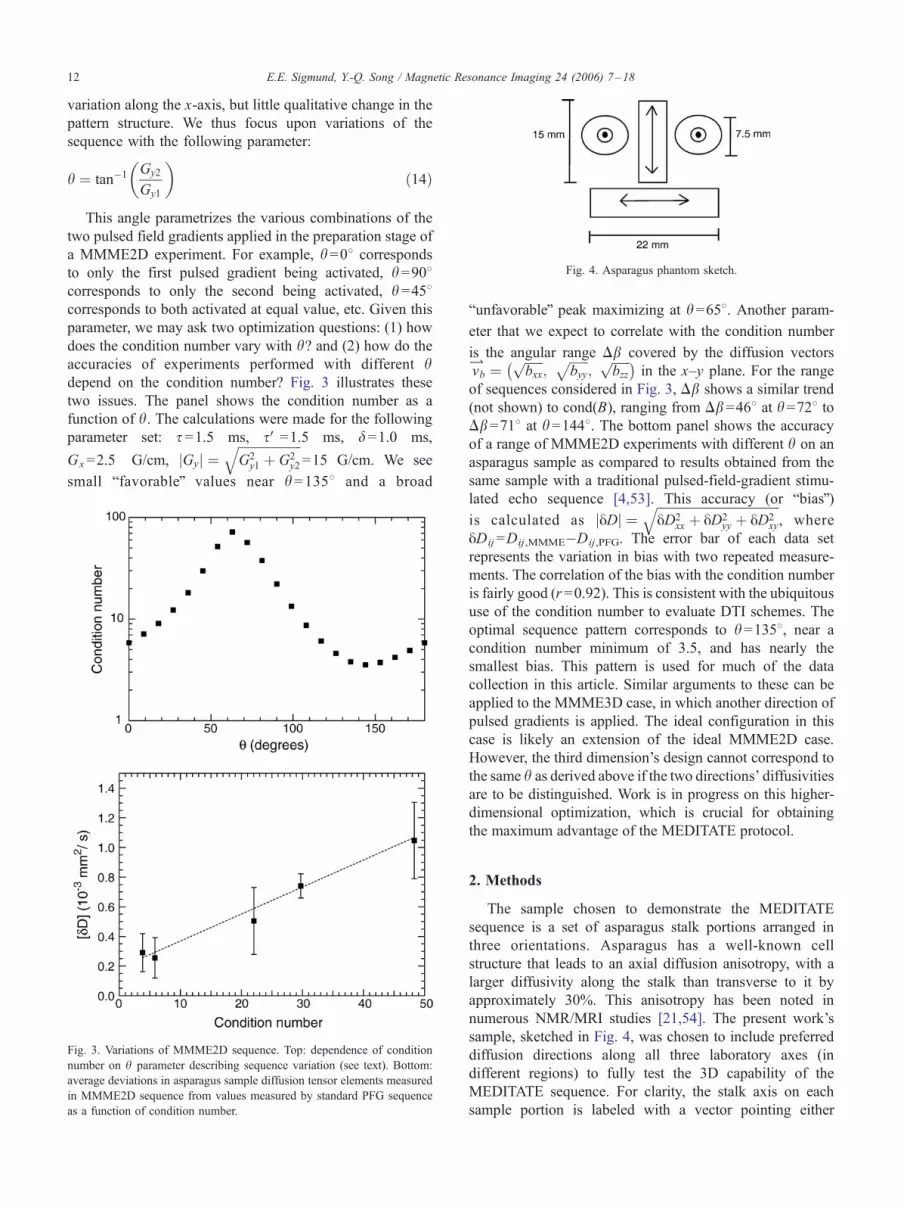
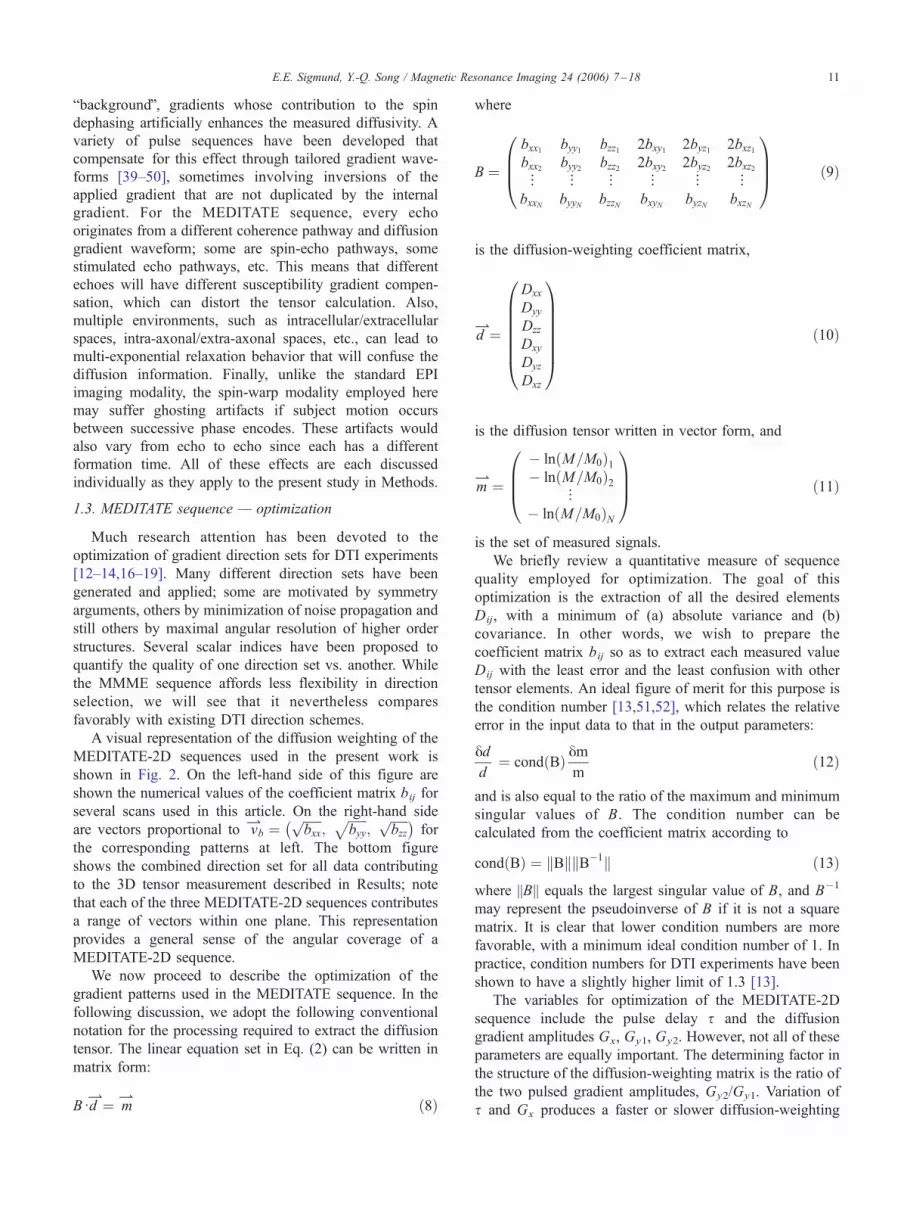
Fig. 4. Asparagus phantom sketch.


variation along the x-axis, but little qualitative change in the

pattern structure. We thus focus upon variations of the

sequence with the following parameter:

h ¼ tan�1 Gy2

Gy1

��ð14Þ

This angle parametrizes the various combinations of the

two pulsed field gradients applied in the preparation stage of

a MMME2D experiment. For example, h=08 corresponds

to only the first pulsed gradient being activated, h=908corresponds to only the second being activated, h=458corresponds to both activated at equal value, etc. Given this

parameter, we may ask two optimization questions: (1) how

does the condition number vary with h? and (2) how do the

accuracies of experiments performed with different hdepend on the condition number? Fig. 3 illustrates these

two issues. The panel shows the condition number as a

function of h. The calculations were made for the following

parameter set: s=1.5 ms, sV=1.5 ms, d=1.0 ms,

Gx=2.5 G/cm, jGyj ¼ffiffiffiffiffiffiffiffiffiffiffiffiffiffiffiffiffiffiffiffiG2

y1 þ G2y2

q=15 G/cm. We see

small bfavorableQ values near h=1358 and a broad

Fig. 3. Variations of MMME2D sequence. Top: dependence of condition

number on h parameter describing sequence variation (see text). Bottom:

average deviations in asparagus sample diffusion tensor elements measured

in MMME2D sequence from values measured by standard PFG sequence

as a function of condition number.

bunfavorableQ peak maximizing at h=658. Another param-

eter that we expect to correlate with the condition number

is the angular range Db covered by the diffusion vectorstvb ¼

ffiffiffiffiffiffibxx

p;

ffiffiffiffiffiffibyy

p;

ffiffiffiffiffiffibzz

p� �in the x–y plane. For the range

of sequences considered in Fig. 3, Db shows a similar trend

(not shown) to cond(B), ranging from Db=468 at h=728 toDb=718 at h=1448. The bottom panel shows the accuracy

of a range of MMME2D experiments with different h on an

asparagus sample as compared to results obtained from the

same sample with a traditional pulsed-field-gradient stimu-

lated echo sequence [4,53]. This accuracy (or bbiasQ)is calculated as jyDj ¼

ffiffiffiffiffiffiffiffiffiffiffiffiffiffiffiffiffiffiffiffiffiffiffiffiffiffiffiffiffiffiffiffiffiffiffiffiffiffiffiyD2

xx þ yD2yy þ yD2

xy

q, where

yDij=Dij,MMME�Dij,PFG. The error bar of each data set

represents the variation in bias with two repeated measure-

ments. The correlation of the bias with the condition number

is fairly good (r=0.92). This is consistent with the ubiquitous

use of the condition number to evaluate DTI schemes. The

optimal sequence pattern corresponds to h=1358, near a

condition number minimum of 3.5, and has nearly the

smallest bias. This pattern is used for much of the data

collection in this article. Similar arguments to these can be

applied to the MMME3D case, in which another direction of

pulsed gradients is applied. The ideal configuration in this

case is likely an extension of the ideal MMME2D case.

However, the third dimension’s design cannot correspond to

the same h as derived above if the two directions’ diffusivities

are to be distinguished. Work is in progress on this higher-

dimensional optimization, which is crucial for obtaining

the maximum advantage of the MEDITATE protocol.

2. Methods

The sample chosen to demonstrate the MEDITATE

sequence is a set of asparagus stalk portions arranged in

three orientations. Asparagus has a well-known cell

structure that leads to an axial diffusion anisotropy, with a

larger diffusivity along the stalk than transverse to it by

approximately 30%. This anisotropy has been noted in

numerous NMR/MRI studies [21,54]. The present work’s

sample, sketched in Fig. 4, was chosen to include preferred

diffusion directions along all three laboratory axes (in

different regions) to fully test the 3D capability of the

MEDITATE sequence. For clarity, the stalk axis on each

sample portion is labeled with a vector pointing either

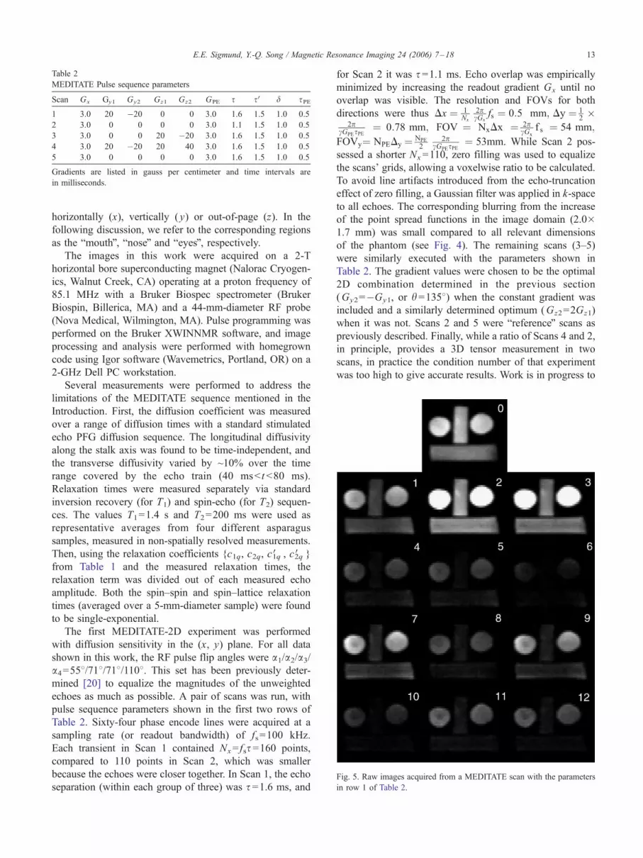
Table 2

MEDITATE Pulse sequence parameters

Scan Gx Gy1 Gy2 Gz1 Gz2 GPE s sV d sPE

1 3.0 20 �20 0 0 3.0 1.6 1.5 1.0 0.5

2 3.0 0 0 0 0 3.0 1.1 1.5 1.0 0.5

3 3.0 0 0 20 �20 3.0 1.6 1.5 1.0 0.5

4 3.0 20 �20 20 40 3.0 1.6 1.5 1.0 0.5

5 3.0 0 0 0 0 3.0 1.6 1.5 1.0 0.5

Gradients are listed in gauss per centimeter and time intervals are

in milliseconds.

Fig. 5. Raw images acquired from a MEDITATE scan with the parameters

in row 1 of Table 2.


horizontally (x), vertically ( y) or out-of-page (z). In the

following discussion, we refer to the corresponding regions

as the bmouthQ, bnoseQ and beyesQ, respectively.The images in this work were acquired on a 2-T

horizontal bore superconducting magnet (Nalorac Cryogen-

ics, Walnut Creek, CA) operating at a proton frequency of

85.1 MHz with a Bruker Biospec spectrometer (Bruker

Biospin, Billerica, MA) and a 44-mm-diameter RF probe

(Nova Medical, Wilmington, MA). Pulse programming was

performed on the Bruker XWINNMR software, and image

processing and analysis were performed with homegrown

code using Igor software (Wavemetrics, Portland, OR) on a

2-GHz Dell PC workstation.

Several measurements were performed to address the

limitations of the MEDITATE sequence mentioned in the

Introduction. First, the diffusion coefficient was measured

over a range of diffusion times with a standard stimulated

echo PFG diffusion sequence. The longitudinal diffusivity

along the stalk axis was found to be time-independent, and

the transverse diffusivity varied by ~10% over the time

range covered by the echo train (40 msb tb80 ms).

Relaxation times were measured separately via standard

inversion recovery (for T1) and spin-echo (for T2) sequen-

ces. The values T1=1.4 s and T2=200 ms were used as

representative averages from four different asparagus

samples, measured in non-spatially resolved measurements.

Then, using the relaxation coefficients {c1q, c2q, c1qV , c2qV }

from Table 1 and the measured relaxation times, the

relaxation term was divided out of each measured echo

amplitude. Both the spin–spin and spin–lattice relaxation

times (averaged over a 5-mm-diameter sample) were found

to be single-exponential.

The first MEDITATE-2D experiment was performed

with diffusion sensitivity in the (x, y) plane. For all data

shown in this work, the RF pulse flip angles were a1/a2/a3/a4=558/718/718/1108. This set has been previously deter-

mined [20] to equalize the magnitudes of the unweighted

echoes as much as possible. A pair of scans was run, with

pulse sequence parameters shown in the first two rows of

Table 2. Sixty-four phase encode lines were acquired at a

sampling rate (or readout bandwidth) of fs=100 kHz.

Each transient in Scan 1 contained Nx= fss=160 points,

compared to 110 points in Scan 2, which was smaller

because the echoes were closer together. In Scan 1, the echo

separation (within each group of three) was s=1.6 ms, and

for Scan 2 it was s=1.1 ms. Echo overlap was empirically

minimized by increasing the readout gradient Gx until no

overlap was visible. The resolution and FOVs for both

directions were thus Dx ¼ 1Nx

2pcGx

fs ¼ 0:5 mm; Dy ¼ 12�

2pcGPEsPE

¼ 0:78 mm; FOV ¼ NxDx ¼ 2pcGx

f s ¼ 54 mm;

FOVy¼ NPEDy ¼ NPE

22p

cGPEsPE¼ 53mm. While Scan 2 pos-

sessed a shorter Nx=110, zero filling was used to equalize

the scans’ grids, allowing a voxelwise ratio to be calculated.

To avoid line artifacts introduced from the echo-truncation

effect of zero filling, a Gaussian filter was applied in k-space

to all echoes. The corresponding blurring from the increase

of the point spread functions in the image domain (2.0�1.7 mm) was small compared to all relevant dimensions

of the phantom (see Fig. 4). The remaining scans (3–5)

were similarly executed with the parameters shown in

Table 2. The gradient values were chosen to be the optimal

2D combination determined in the previous section

(Gy2=�Gy1, or h=1358) when the constant gradient was

included and a similarly determined optimum (Gz2=2Gz1)

when it was not. Scans 2 and 5 were breferenceQ scans as

previously described. Finally, while a ratio of Scans 4 and 2,

in principle, provides a 3D tensor measurement in two

scans, in practice the condition number of that experiment

was too high to give accurate results. Work is in progress to

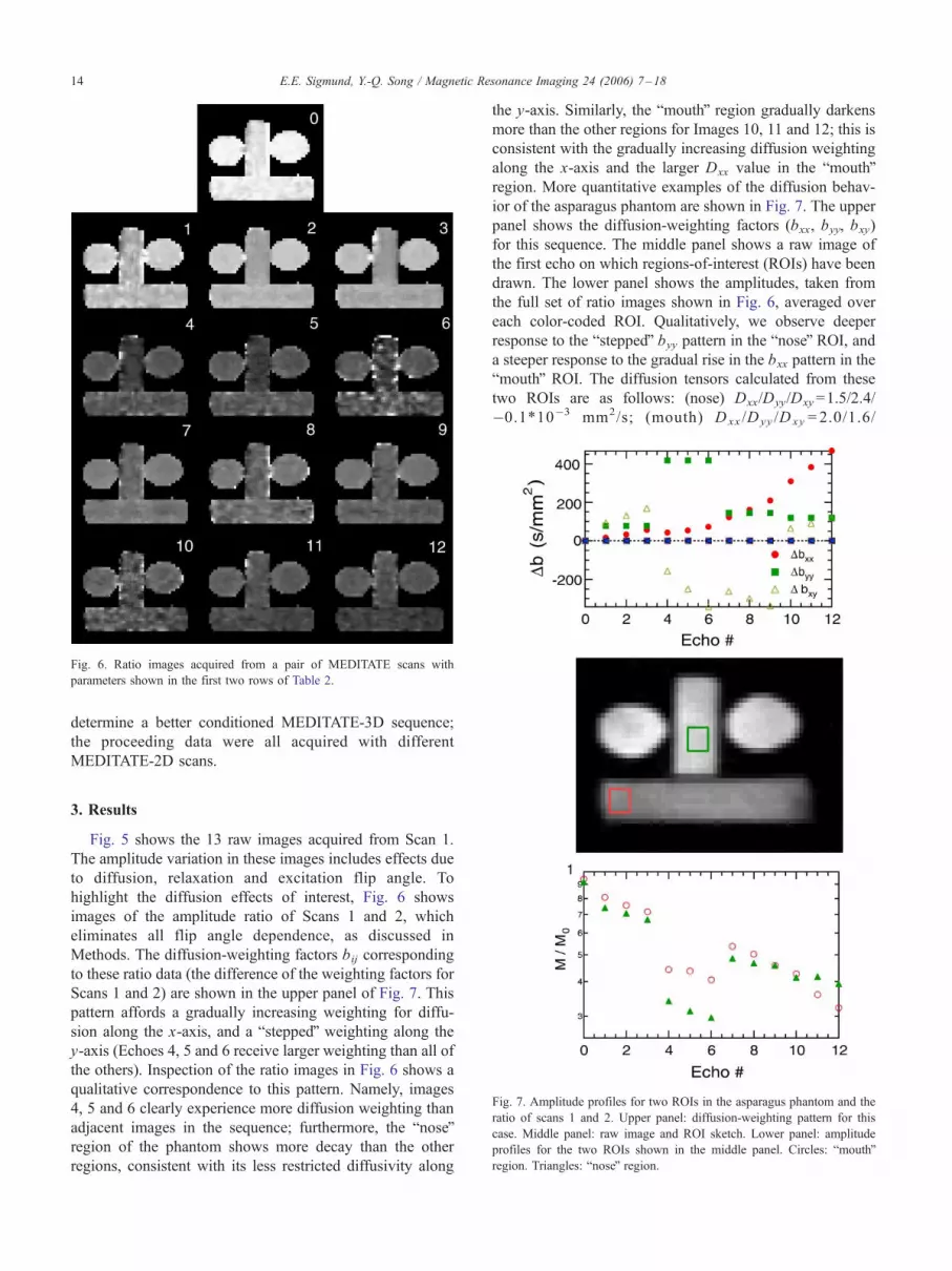
Fig. 6. Ratio images acquired from a pair of MEDITATE scans with

parameters shown in the first two rows of Table 2.


determine a better conditioned MEDITATE-3D sequence;

the proceeding data were all acquired with different

MEDITATE-2D scans.

Fig. 7. Amplitude profiles for two ROIs in the asparagus phantom and the

ratio of scans 1 and 2. Upper panel: diffusion-weighting pattern for this

case. Middle panel: raw image and ROI sketch. Lower panel: amplitude

profiles for the two ROIs shown in the middle panel. Circles: bmouthQregion. Triangles: bnoseQ region.

3. Results

Fig. 5 shows the 13 raw images acquired from Scan 1.

The amplitude variation in these images includes effects due

to diffusion, relaxation and excitation flip angle. To

highlight the diffusion effects of interest, Fig. 6 shows

images of the amplitude ratio of Scans 1 and 2, which

eliminates all flip angle dependence, as discussed in

Methods. The diffusion-weighting factors bij corresponding

to these ratio data (the difference of the weighting factors for

Scans 1 and 2) are shown in the upper panel of Fig. 7. This

pattern affords a gradually increasing weighting for diffu-

sion along the x-axis, and a bsteppedQ weighting along the

y-axis (Echoes 4, 5 and 6 receive larger weighting than all of

the others). Inspection of the ratio images in Fig. 6 shows a

qualitative correspondence to this pattern. Namely, images

4, 5 and 6 clearly experience more diffusion weighting than

adjacent images in the sequence; furthermore, the bnoseQregion of the phantom shows more decay than the other

regions, consistent with its less restricted diffusivity along

the y-axis. Similarly, the bmouthQ region gradually darkens

more than the other regions for Images 10, 11 and 12; this is

consistent with the gradually increasing diffusion weighting

along the x-axis and the larger Dxx value in the bmouthQregion. More quantitative examples of the diffusion behav-

ior of the asparagus phantom are shown in Fig. 7. The upper

panel shows the diffusion-weighting factors (bxx, byy, bxy)

for this sequence. The middle panel shows a raw image of

the first echo on which regions-of-interest (ROIs) have been

drawn. The lower panel shows the amplitudes, taken from

the full set of ratio images shown in Fig. 6, averaged over

each color-coded ROI. Qualitatively, we observe deeper

response to the bsteppedQ byy pattern in the bnoseQ ROI, anda steeper response to the gradual rise in the bxx pattern in the

bmouthQ ROI. The diffusion tensors calculated from these

two ROIs are as follows: (nose) Dxx/Dyy/Dxy=1.5/2.4/

�0.1*10�3 mm2/s; (mouth) Dxx /Dyy /Dxy = 2.0/1.6/

Dxx Dyy Dzz Directivity

3.0

2.5

2.0

1.5

1.0

0.5

0.0

D (1

0-3 m

m2/s)

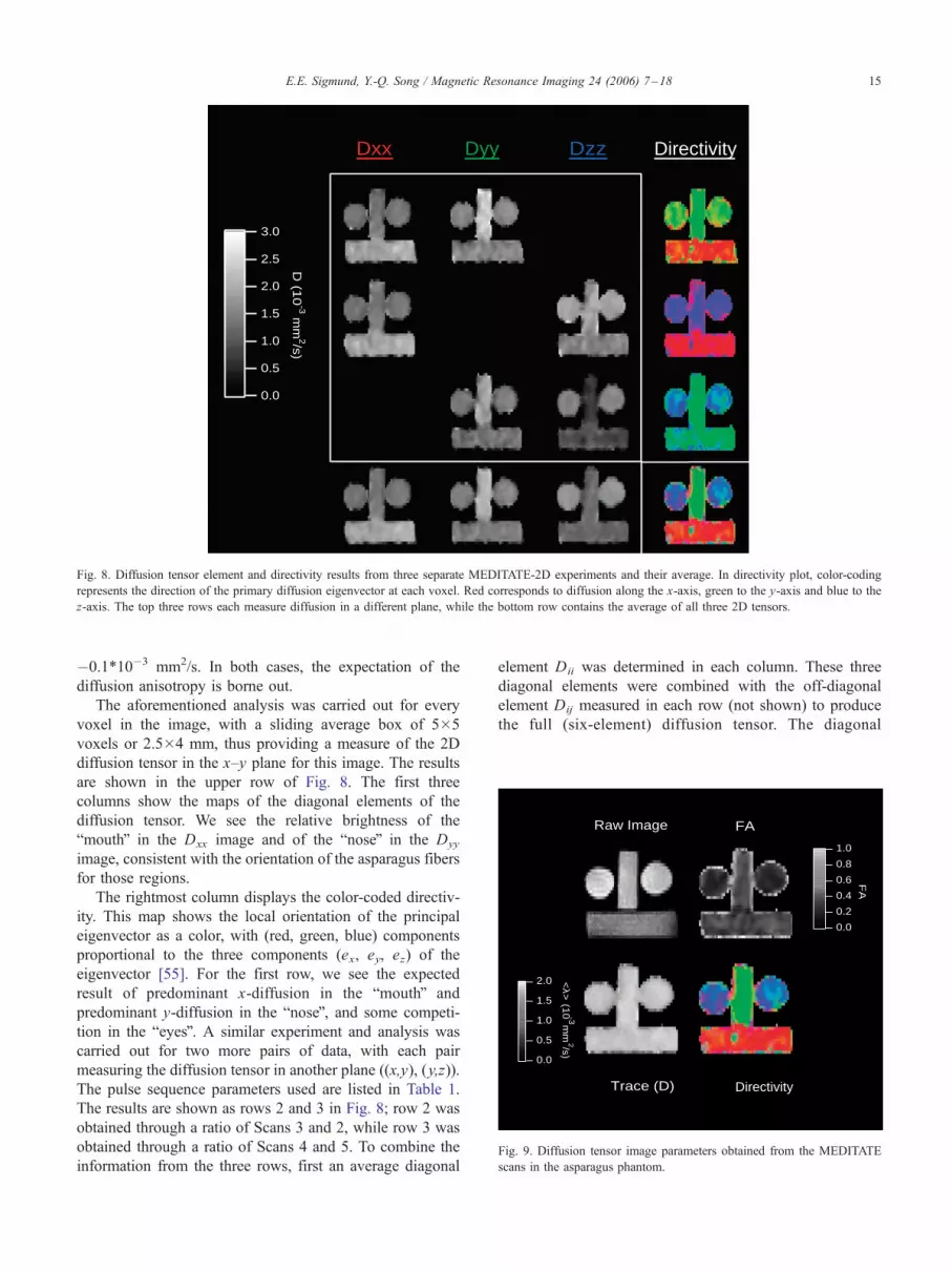
Fig. 8. Diffusion tensor element and directivity results from three separate MEDITATE-2D experiments and their average. In directivity plot, color-coding

represents the direction of the primary diffusion eigenvector at each voxel. Red corresponds to diffusion along the x-axis, green to the y-axis and blue to the

z-axis. The top three rows each measure diffusion in a different plane, while the bottom row contains the average of all three 2D tensors.

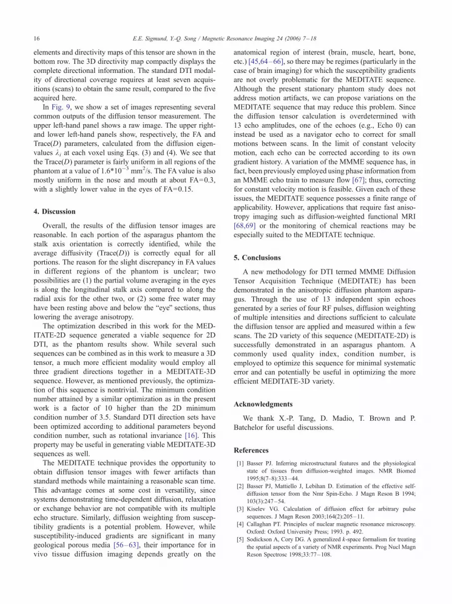
Raw Image FA

Trace (D) Directivity

1.0

0.8

0.6

0.4

0.2

0.0

FA

2.0

1.5

1.0

0.5

0.0

<λ>

(10 m

m2/s)

-3

Fig. 9. Diffusion tensor image parameters obtained from the MEDITATE

scans in the asparagus phantom.


�0.1*10�3 mm2/s. In both cases, the expectation of the

diffusion anisotropy is borne out.

The aforementioned analysis was carried out for every

voxel in the image, with a sliding average box of 5�5

voxels or 2.5�4 mm, thus providing a measure of the 2D

diffusion tensor in the x–y plane for this image. The results

are shown in the upper row of Fig. 8. The first three

columns show the maps of the diagonal elements of the

diffusion tensor. We see the relative brightness of the

bmouthQ in the Dxx image and of the bnoseQ in the Dyy

image, consistent with the orientation of the asparagus fibers

for those regions.

The rightmost column displays the color-coded directiv-

ity. This map shows the local orientation of the principal

eigenvector as a color, with (red, green, blue) components

proportional to the three components (ex, ey, ez) of the

eigenvector [55]. For the first row, we see the expected

result of predominant x-diffusion in the bmouthQ and

predominant y-diffusion in the bnoseQ, and some competi-

tion in the beyesQ. A similar experiment and analysis was

carried out for two more pairs of data, with each pair

measuring the diffusion tensor in another plane ((x,y), (y,z)).

The pulse sequence parameters used are listed in Table 1.

The results are shown as rows 2 and 3 in Fig. 8; row 2 was

obtained through a ratio of Scans 3 and 2, while row 3 was

obtained through a ratio of Scans 4 and 5. To combine the

information from the three rows, first an average diagonal

element Dii was determined in each column. These three

diagonal elements were combined with the off-diagonal

element Dij measured in each row (not shown) to produce

the full (six-element) diffusion tensor. The diagonal


elements and directivity maps of this tensor are shown in the

bottom row. The 3D directivity map compactly displays the

complete directional information. The standard DTI modal-

ity of directional coverage requires at least seven acquis-

itions (scans) to obtain the same result, compared to the five

acquired here.

In Fig. 9, we show a set of images representing several

common outputs of the diffusion tensor measurement. The

upper left-hand panel shows a raw image. The upper right-

and lower left-hand panels show, respectively, the FA and

Trace(D) parameters, calculated from the diffusion eigen-

values ki at each voxel using Eqs. (3) and (4). We see that

the Trace(D) parameter is fairly uniform in all regions of the

phantom at a value of 1.6*10�3 mm2/s. The FA value is also

mostly uniform in the nose and mouth at about FA=0.3,

with a slightly lower value in the eyes of FA=0.15.

4. Discussion

Overall, the results of the diffusion tensor images are

reasonable. In each portion of the asparagus phantom the

stalk axis orientation is correctly identified, while the

average diffusivity (Trace(D)) is correctly equal for all

portions. The reason for the slight discrepancy in FA values

in different regions of the phantom is unclear; two

possibilities are (1) the partial volume averaging in the eyes

is along the longitudinal stalk axis compared to along the

radial axis for the other two, or (2) some free water may

have been resting above and below the beyeQ sections, thuslowering the average anisotropy.

The optimization described in this work for the MED-

ITATE-2D sequence generated a viable sequence for 2D

DTI, as the phantom results show. While several such

sequences can be combined as in this work to measure a 3D

tensor, a much more efficient modality would employ all

three gradient directions together in a MEDITATE-3D

sequence. However, as mentioned previously, the optimiza-

tion of this sequence is nontrivial. The minimum condition

number attained by a similar optimization as in the present

work is a factor of 10 higher than the 2D minimum

condition number of 3.5. Standard DTI direction sets have

been optimized according to additional parameters beyond

condition number, such as rotational invariance [16]. This

property may be useful in generating viable MEDITATE-3D

sequences as well.

The MEDITATE technique provides the opportunity to

obtain diffusion tensor images with fewer artifacts than

standard methods while maintaining a reasonable scan time.

This advantage comes at some cost in versatility, since

systems demonstrating time-dependent diffusion, relaxation

or exchange behavior are not compatible with its multiple

echo structure. Similarly, diffusion weighting from suscep-

tibility gradients is a potential problem. However, while

susceptibility-induced gradients are significant in many

geological porous media [56–63], their importance for in

vivo tissue diffusion imaging depends greatly on the

anatomical region of interest (brain, muscle, heart, bone,

etc.) [45,64–66], so there may be regimes (particularly in the

case of brain imaging) for which the susceptibility gradients

are not overly problematic for the MEDITATE sequence.

Although the present stationary phantom study does not

address motion artifacts, we can propose variations on the

MEDITATE sequence that may reduce this problem. Since

the diffusion tensor calculation is overdetermined with

13 echo amplitudes, one of the echoes (e.g., Echo 0) can

instead be used as a navigator echo to correct for small

motions between scans. In the limit of constant velocity

motion, each echo can be corrected according to its own

gradient history. A variation of the MMME sequence has, in

fact, been previously employed using phase information from

an MMME echo train to measure flow [67]; thus, correcting

for constant velocity motion is feasible. Given each of these

issues, the MEDITATE sequence possesses a finite range of

applicability. However, applications that require fast aniso-

tropy imaging such as diffusion-weighted functional MRI

[68,69] or the monitoring of chemical reactions may be

especially suited to the MEDITATE technique.

5. Conclusions

A new methodology for DTI termed MMME Diffusion

Tensor Acquisition Technique (MEDITATE) has been

demonstrated in the anisotropic diffusion phantom aspara-

gus. Through the use of 13 independent spin echoes

generated by a series of four RF pulses, diffusion weighting

of multiple intensities and directions sufficient to calculate

the diffusion tensor are applied and measured within a few

scans. The 2D variety of this sequence (MEDITATE-2D) is

successfully demonstrated in an asparagus phantom. A

commonly used quality index, condition number, is

employed to optimize this sequence for minimal systematic

error and can potentially be useful in optimizing the more

efficient MEDITATE-3D variety.

Acknowledgments

We thank X.-P. Tang, D. Madio, T. Brown and P.

Batchelor for useful discussions.

References

[1] Basser PJ. Inferring microstructural features and the physiological

state of tissues from diffusion-weighted images. NMR Biomed

1995;8(7–8):333–44.

[2] Basser PJ, Mattiello J, Lebihan D. Estimation of the effective self-

diffusion tensor from the Nmr Spin-Echo. J Magn Reson B 1994;

103(3):247–54.

[3] Kiselev VG. Calculation of diffusion effect for arbitrary pulse

sequences. J Magn Reson 2003;164(2):205–11.

[4] Callaghan PT. Principles of nuclear magnetic resonance microscopy.

Oxford7 Oxford University Press; 1993. p. 492.

[5] Sodickson A, Cory DG. A generalized k-space formalism for treating

the spatial aspects of a variety of NMR experiments. Prog Nucl Magn

Reson Spectrosc 1998;33:77–108.


[6] Inglis BA, Bossart EL, Buckley DL, Wirth III ED, Mareci TH.

Visualization of neural tissue water compartments using biexponential

diffusion tensor MRI. Magn Reson Med 2001;45(4):580–7.

[7] StehlingMK, Turner R,Mansfield P. Echo-planar imaging—magnetic-

resonance-imaging in a fraction of a second. Science 1991;254(5028):

43–50.

[8] Deoni SCL, Peters TM, Rutt BK. Quantitative diffusion imaging

with steady-state free precession. Magn Reson Med 2004;51(2):

428–33.

[9] Wu EX, Buxton RB. Effect of diffusion on the steady-state

magnetization with pulsed field gradients. J Magn Reson 1990;

90(2):243–53.

[10] Zur Y, Bosak E, Kaplan N. A new diffusion SSFP imaging technique.

Magn Reson Med 1997;37(5):716–22.

[11] Gulani V, Iwamoto GA, Jiang H, Shimony JS, Webb AG, Lauterbur

PC. A multiple echo pulse sequence for diffusion tensor imaging and

its application in excised spinal cords. Magn Reson Med 1997;

38:868–73.

[12] Papadakis NG, Xing D, Huang CL-H, Hall LD, Carpenter TA. A

comparative study of acquisition schemes for diffusion tensor imaging

using MRI. J Magn Reson 1999;137(2):67–82.

[13] Skare S, Hedehus M, Moseley ME, Li TQ. Condition number as a

measure of noise performance of diffusion tensor data acquisition

schemes with MRI. J Magn Reson 2000;147(2):340–52.

[14] Jones DK, Horsfield MA, Simmons A. Optimal strategies for

measuring diffusion in anisotropic systems by magnetic resonance

imaging. Magn Reson Med 1999;42(3):515–25.

[15] Tuch DS, Reese TG, Wiegell MR, Makris N, Belliveau JW, Wedeen

VJ. High angular resolution diffusion imaging reveals intravoxel

white matter fiber heterogeneity. Magn Reson Med 2002;48:577–82.

[16] Batchelor PG, Atkinson D, Hill DLG, Calmante F, Connelly A.

Anisotropic noise propagation in diffusion tensor MRI sampling

schemes. Magn Reson Med 2003;49(6):1143–51.

[17] Hasan KM, Parker DL, Alexander AL. Comparison of gradient

encoding schemes for diffusion-tensor MRI. J Magn Reson Imaging

2001;13(5):769–80.

[18] Ozcan A. (Mathematical) Necessary conditions for the selection of

gradient vectors in DTI. J Magn Reson 2004;172:238–41.

[19] Poonawalla AH, Zhou XHJ. Analytical error propagation in

diffusion anisotropy calculations. J Magn Reson Imaging 2004;

19(4):489–98.

[20] Song Y-Q, Tang X-P. A one-shot method for measurement of

diffusion. J Magn Reson 2004;170:136–48.

[21] Tang X-P, Sigmund EE, Song Y-Q. Simultaneous measurement of

diffusion along multiple directions. J Am Chem Soc 2004;

126(50):16336–7.

[22] Counsell CJ. PREVIEW: a new ultrafast imaging sequence requiring

minimal gradient switching. Magn Reson Imaging 1993;11:603–16.

[23] Heid O, Deimling M, Huk W. QUEST—A quick echo split NMR

imaging technique. Magn Reson Med 1993;29:280–3.

[24] Ong H, Chin C-L, Wehrli SL, Tang X-P, Wehrli FW. A new approach

for simultaneous measurement of ADC and T_2 from echoes

generated via multiple coherence pathways. J Magn Reson 2005;

173:153–9.

[25] Doran SJ, Decorps M. A robust, single-shot method for measuring

diffusion coefficients using the bBurstQ sequence. J Magn Reson, Ser

A 1995;117:311.

[26] Doran SJ, Jakob P, Decorps M. Rapid repetition of the bBurstQsequence: the role of diffusion and consequences for imaging. Magn

Reson Med 1996;35(4):547–53.

[27] Lowe IJ, Wysong RE. DANTE ultrafast imaging sequence (DUFIS).

J Magn Reson B 1993;101:106.

[28] Stamps JP, Ottink B, Visser JM, van Duynhoven JPM, Hulst R.

Difftrain: a novel approach to a true spectroscopic single-scan

diffusion measurement. J Magn Reson 2001;151:28–31.

[29] Chin CL, Tang XP, Bouchard LS, Saha PK, Warren WS, Wehrli FW.

Isolating quantum coherences in structural imaging using intermolec-

ular double-quantum coherence MRI. J Magn Reson 2003;165(2):

309–14.

[30] Shannon KL, Branca RT, Galiana G, Cenzano S, Bouchard LS,

Soboyejo W, et al. Simultaneous acquisition of multiple orders of

intermolecular multiple-quantum coherence images in vivo. Magn

Reson Imaging 2004;22(10):1407–12.

[31] Haacke EM, Brown RW, Thompson MR, Venkatesan R. Magnetic

resonance imaging: physical principles and sequence design. New

York7 Wiley-Liss; 1999.

[32] Hurlimann MD. Diffusion and relaxation effects in general stray field

NMR experiments. J Magn Reson 2001;148:367–78.

[33] Song YQ. Categories of coherence pathways for the CPMG sequence.

J Magn Reson 2002;157(1):82–91.

[34] Hurlimann MD, Helmer KG, Latour LL, Sotak CH. Restricted

diffusion in sedimentary rocks. Determination of surface-to-volume

ratio and surface relaxivity. J Magn Reson, Ser A 1994;111:169–78.

[35] McCall KR, Johnson DL, Guyer RA. Magnetization evolution in

connected pore system: II. Pulse field gradient NMR and pore-space

geometry. Phys Rev, B 1993;48:5997–6006.

[36] Mitra PP, Sen PN, Schwartz LM. Short-time behavior of the diffusion

coefficient as a geometrical probe of porous media. Phys Rev, B

1993;47:8565.

[37] Parsons EC, Does MD, Gore JC. Modified oscillating gradient pulses

for direct sampling of the diffusion spectrum suitable for imaging

sequences. Magn Reson Imaging 2003;21(3–4):279–85.

[38] Sen PN. Time-dependent diffusion coefficient as a probe of geometry.

Concepts Magn Reson 2004;23:1–21.

[39] Williams WD, Seymour EFW, Cotts RM. A pulsed-gradient multiple-

spin-echo NMR technique for measuring diffusion in the presence

of background magnetic field gradients. J Magn Reson 1978;31:

271–82.

[40] Karlicek JRF, Lowe IJ. A modified pulsed gradient technique for

measuring diffusion in the presence of large background gradients.

J Magn Reson (1969) 1980;37(1):75.

[41] Corns RM, Hoch MJR, Sun T, Markert JT. Pulsed field gradient

stimulated echo methods for improved NMR diffusion measurements

in heterogeneous systems. J Magn Reson 1989;83(2):252.

[42] Latour LL, Li LM, Sotak CH. Improved PFG stimulated-echo method

for the measurement of diffusion in inhomogeneous fields. J Magn

Reson B 1993;101(1):72.

[43] Lian J, Williams DS, Lowe IJ. Magnetic resonance imaging of

diffusion in the presence of background gradients and imaging of

background gradients. J Magn Reson, Ser A 1994;106(1):65.

[44] Trudeau JD, Dixon WT, Hawkins J. The effect of inhomogeneous

sample susceptibility on measured diffusion anisotropy using NMR

imaging. J Magn Reson B 1995;108(1):22.

[45] Clark CA, Barker GJ, Tofts PS. An in vivo evaluation of the effects

of local magnetic susceptibility-induced gradients on water

diffusion measurements in human brain. J Magn Reson 1999;141(1):

52–61.

[46] Johnson CS. Diffusion ordered nuclear magnetic resonance spectros-

copy: principles and applications. Prog Nucl Magn Reson Spectrosc

1999;34(3–4):203–56.

[47] Seland JG, Sorland GH, Zick K, Hafskjold B. Diffusion measure-

ments at long observation times in the presence of spatially variable

internal magnetic field gradients. J Magn Reson 2000;146(1):14–9.

[48] Mohoric A. A modified PGSE for measuring diffusion in the pre-

sence of static magnetic field gradients. J Magn Reson 2005;174(2):

223–8.

[49] Galvosas P, Stallmach F, Karger J. Background gradient suppression

in stimulated echo NMR diffusion studies using magic pulsed field

gradient ratios. J Magn Reson 2004;166(2):164.

[50] Sun PZ, Seland JG, Cory D. Background gradient suppression in

pulsed gradient stimulated echo measurements. J Magn Reson 2003;

161(2):168.

[51] Press WH, Teukolsky SA, Vetterling WT, Flannery BP. Numerical

recipes in C. Cambridge7 Cambridge University Press; 1997.


[52] Strang G. Introduction to linear Algebra. Wellesley, MA7 Wellesley-

Cambridge Press; 1998.

[53] Stejskal EO, Tanner JE. Spin diffusion measurements: spin echoes in

the presence of a time-dependent field gradient. J Chem Phys 1965;

42:288–92.

[54] Boujraf S, Luypaert R, Eisendrath H, Osteaux M. Echo planar

magnetic resonance imaging of anisotropic diffusion in asparagus

stems. Magn Reson Mater Phys Biol Med 2001;13:82–90.

[55] Pajevic S, Pierpaoli C. Color schemes to represent the orientation of

anisotropic tissues from diffusion tensor data: Application to white

matter fiber tract mapping in the human brain. Magn Reson Med

1999;42(3):526–40.

[56] Audoly B, Sen PN, Ryu S, Song Y-Q. Correlation functions for

inhomogeneous magnetic field in random media with application to a

dense random pack of spheres. J Magn Reson 2003;164:154–9.

[57] Borgia GC, Brown RJS, Fantazzini P. The effect of diffusion and

susceptibility differences on T2 measurements for fluid in porous

media and biological tissues. Magn Reson Imaging 1996;14:731–6.

[58] Hurlimann MD. Effective gradients in porous media due to

susceptibility differences. J Magn Reson 1998;131:232–40.

[59] Petkovic J, Huinink HP, Pel L, Kopinga K. Diffusion in porous

building materials with high internal magnetic field gradients. J Magn

Reson 2004;167:97–106.

[60] Seland JG, Washburn KE, Anthonsen HW, Krane J. Correlations

between diffusion, internal magnetic field gradients, and transverse

relaxation in porous systems containing oil and water. Phys Rev, E

2004;70(5):051305.

[61] Sen PN, Axelrod S. Inhomogeneity in local magnetic field due to

susceptibility contrast. J Appl Phys 1999;86:4548–54.

[62] Song Y-Q. Using internal magnetic fields to obtain pore size

distributions of porous media. Concepts Magn Reson 2003;18A(2):

97–110.

[63] Song Y-Q, Ryu S, Sen PN. Determining multiple length scales in

rocks. Nature (London) 2000;406:178–81.

[64] Kiselev VG. Effect of magnetic field gradients induced by microvas-

culature on NMR measurements of molecular self-diffusion in

biological tissues. J Magn Reson 2004;170(2):228–35.

[65] Majumdar S, Gore JC. Studies of diffusion in random fields produced

by variations in susceptibility. J Magn Reson 1988;78:41–55.

[66] Zhong J, Kennan RP, Gore JC. Effects of susceptibility variations on

NMR measurements of diffusion. J Magn Reson 1991;95(2):267.

[67] Song YQ, Scheven UM. An NMR technique for rapid measurement of

flow. J Magn Reson 2005;172(1):31–5.

[68] Song AW, Harshbarger T, Li TL, Kim KH, Ugurbil K, Mori S, et al.

Functional activation using apparent diffusion coefficient-dependent

contrast allows better spatial localization to the neuronal activity:

evidence using diffusion tensor imaging and fiber tracking. Neuro-

Image 2003;20(2):955–61.

[69] Song AW, Wong EC, Tan SG, Hyde JS. Diffusion weighted fMRI at

1.5 T. Magn Reson Med 1996;35(2):155–8.

multiple echo diffusion tensor acquisition technique

Documents