stability and bifurcation of predator-prey
TRANSCRIPT

STABILITY AND BIFURCATION OF
PREDATOR-PREY MODELS WITH THE
ALLEE EFFECT
SINAN KAPCAK
JULY 2013

STABILITY AND BIFURCATION OF
PREDATOR-PREY MODELS WITH THE
ALLEE EFFECT
a dissertation submitted to
the graduate school of natural
and applied sciences of
izmir university of economics
by
SINAN KAPCAK
in partial fulfillment of the requirements
for the degree of doctor of philosophy
in the graduate school of natural and applied sciences
JULY 2013


ABSTRACT
STABILITY AND BIFURCATION OF
PREDATOR-PREY MODELS WITH THE ALLEE
EFFECT
SINAN KAPCAK
Ph.D. in Applied Mathematics and Statistics
Graduate School of Natural and Applied Sciences
Supervisor: Prof. Dr. Unal Ufuktepe
Co-Supervisor: Prof. Dr. Saber Elaydi
July 2013
One of the most well-known model with several interacting populations is
Nicholson-Bailey host-parasitoid model [44]. This is a nonlinear discrete-time
model to a biological system involved two insects, a parasitoid and its host.
Beddington et al investigated a density-dependent version of Nicholson-Bailey
model where the host rate of increase is logistic [4]. Another more realistic version
of the system was studied by Hone, Irle, and Thurura where the model displays the
more biologically relevant possibilities that the two populations can asymtotically
approach positive steady-state values or move towards an attracting invariant
curve in the phase plane [21].
This thesis will investigate the generalization of Beddington model and the
Beddington model with Allee effect.
Keywords: discrete dynamical systems, beddington model, allee effect, stability,
invariant curves, bifurcation.
iii
OZ
AV-AVCI MODELLERININ ALLEE ETKISI ALTINDA
STABILITE VE DALLANMASI
SINAN KAPCAK
Uygulamalı Matematik ve Istatistik, Doktora
Fen Bilimleri Enstitusu
Tez Danısmanı: Prof. Dr. Unal Ufuktepe
Ikinci Tez Danısmanı: Prof. Dr. Saber Elaydi
Temmuz 2013
Birbirinden farklı populasyonların etkilesiminin en iyi bilinen orneklerinden
biri Nicholson-Bailey konakcı-parazitoid modelidir [44]. Bu, bir parazitoid ve
konakcısından olusan, dogrusal olmayan bir kesikli-zaman modelidir. Bedding-
ton ve arkadasları, Nicholson-Bailey modelinin, konakcı sayısının lojistik olarak
buyudugu, yogunluga baglı versiyonunu arastırmıslardır [4]. Yine aynı sistemin
gercekci baska bir hali Hone, Irle ve Thurura tarafından modellenmistir. Bu mod-
elde, faz duzleminde, iki populasyon da asimtotik olarak sabit noktalara veya
invaryant bir egriye yakınsayabiliyor [21].
Bu tezde, Beddington modelinin genellestirilmis halini ve bu modelin Allee
etkisi altındaki dinamiklerini arastıracagız.
Anahtar Kelimeler : kesikli dinamik sistemler, beddington modeli, allee etkisi,
stabilite, invaryant egriler, dallanma.
iv

ACKNOWLEDGEMENT
I would like to express my very great appreciation to Prof. Dr. Unal Ufuktepe
for his patient guidance, enthusiastic encouragement and useful critiques of this
Ph.D. thesis. He is not only supervisor but dear friend. His positive outlook
and confidence in my research inspired me and gave me confidence. I would like
to express my heartfelt gratitude to my co-supervisor Prof. Dr. Saber Elaydi
for his help and support during this research and my visit to Trinity University,
TX, U.S.A. His willingness to give his time so generously has been very much
appreciated.
I would like to express my appreciation to the advice of the committee mem-
bers, Prof. Dr. Murat Adıvar and Assoc. Prof. Dr. Serap Topal, for their
critical comments, which enabled me to notice the weaknesses of my dissertation
and make the necessary improvements according to their comments.
I would like to acknowledge the academic support of Izmir University of Eco-
nomics, in the award of a Postgraduate Studentship. My sincere thanks go to
The Scientific & Technological Research Council of Turkey (TUBITAK) for their
financial support for my visit to Trinity University. I would also like to thank
Trinity University for hosting me during the period the part of this thesis was
written.
Special thanks should be given to my dear friends Assoc. Prof. Gozde Yazgı
Tutuncu, Goknur Giner, Gulder Kemalbay, Nalan Gunduz, Abdulkadir Dogru,
Ugur Akduman, Savas Yucel, and my cousins Emre Bostan, Elif Esra Dom, and
Veysel Bilge for their support and encouragement.
Last but not least, I am greatly indebted to my family who form the backbone
and origin of my happiness. Their love and support without any complaint or
v

vi
regret has enabled me to complete this Ph.D. research.

To my family
vii

TABLE OF CONTENTS
Front Matter i
Abstract . . . . . . . . . . . . . . . . . . . . . . . . . . . . . . . . . . . iii
Oz . . . . . . . . . . . . . . . . . . . . . . . . . . . . . . . . . . . . . . iv
Acknowledgement . . . . . . . . . . . . . . . . . . . . . . . . . . . . . . v
Table of Contents . . . . . . . . . . . . . . . . . . . . . . . . . . . . . . x
List of Tables . . . . . . . . . . . . . . . . . . . . . . . . . . . . . . . . xi
List of Figures . . . . . . . . . . . . . . . . . . . . . . . . . . . . . . . . xiv
1 Introduction 1
2 Preliminaries 4
2.1 Stability of Fixed Points for One-Dimesional Maps . . . . . . . . 4
2.2 Stability of Fixed Points for Two-Dimensional Maps . . . . . . . . 6
2.3 Invariant Manifolds . . . . . . . . . . . . . . . . . . . . . . . . . . 9
2.3.1 Center Manifolds . . . . . . . . . . . . . . . . . . . . . . . 11
2.3.2 Stable and Unstable Manifolds . . . . . . . . . . . . . . . . 13
viii
2.4 Bifurcation . . . . . . . . . . . . . . . . . . . . . . . . . . . . . . 14
2.5 Related Population Models . . . . . . . . . . . . . . . . . . . . . . 17
2.5.1 One-Dimensional Population Models . . . . . . . . . . . . 17
2.5.2 Two-Dimensional Population Models . . . . . . . . . . . . 18
3 Population Models with Allee Effect 28
3.1 Allee Effect . . . . . . . . . . . . . . . . . . . . . . . . . . . . . . 28
3.2 A Predator-prey Model with Allee Effect . . . . . . . . . . . . . . 30
3.2.1 Stability of Fixed Points for System (3.4) . . . . . . . . . . 31
3.2.2 Instability of Exclusion Fixed Point . . . . . . . . . . . . . 32
4 Main Problem 40
4.1 Generalized Beddington Model . . . . . . . . . . . . . . . . . . . 40
4.1.1 Fixed Points . . . . . . . . . . . . . . . . . . . . . . . . . . 41
4.1.2 Stability of Fixed Points for system (4.2) . . . . . . . . . . 49
4.1.3 Stable and Unstable Manifolds . . . . . . . . . . . . . . . . 57
4.1.4 Bifurcation Scenarios . . . . . . . . . . . . . . . . . . . . . 61
4.2 Beddington Model with Allee Effect . . . . . . . . . . . . . . . . . 65
4.2.1 Allee Effect on Parasitoid Population . . . . . . . . . . . . 65
4.2.2 Allee Effect on Host Population . . . . . . . . . . . . . . . 74
5 Conclusion and Further Studies 90
ix

A Mathematica Codes 91
A.1 Cobweb Diagram . . . . . . . . . . . . . . . . . . . . . . . . . . . 91
A.2 Time Series Diagram . . . . . . . . . . . . . . . . . . . . . . . . . 92
A.3 Phase Diagram . . . . . . . . . . . . . . . . . . . . . . . . . . . . 93
A.4 Bifurcation Diagram . . . . . . . . . . . . . . . . . . . . . . . . . 95
B Stability of Fixed Points 97
x

LIST OF TABLES
2.1 Types of bifurcation of fixed points. . . . . . . . . . . . . . . . . . 17
3.1 Allee effect may stabilize or destabilize the system. . . . . . . . . 36
B.1 Stability of Fixed Points for 2-dimensional linear system. . . . . . 98
B.2 Stability of Fixed Points for 2-dimensional linear system. . . . . . 99
B.3 Stability of Fixed Points for 2-dimensional linear system. . . . . . 100
xi

LIST OF FIGURES
2.1 Stable and centre manifolds. . . . . . . . . . . . . . . . . . . . . . 12
2.2 Stable and unstable manifolds. . . . . . . . . . . . . . . . . . . . . 14
2.3 y = R(b+c+cx)c(1+x+bx)
and y = (1 + x)b. . . . . . . . . . . . . . . . . . . . . 24
2.4 z = F (x), z = R. . . . . . . . . . . . . . . . . . . . . . . . . . . . 25
2.5 Phase portrait of system (2.18). . . . . . . . . . . . . . . . . . . . 27
2.6 Phase portrait of the system (2.18). . . . . . . . . . . . . . . . . . 27
3.1 Some orbits of the system (3.4). . . . . . . . . . . . . . . . . . . 33
3.2 Trajectories of the prey-predator system. . . . . . . . . . . . . . 37
3.3 Trajectories of the prey-predator system. . . . . . . . . . . . . . 38
4.1 z = F (x), z = r. . . . . . . . . . . . . . . . . . . . . . . . . . . . . 42
4.2 Regions R1, R2, R3, R4. . . . . . . . . . . . . . . . . . . . . . . . 44
4.3 f(x), g(x). . . . . . . . . . . . . . . . . . . . . . . . . . . . . . . . 45
4.4 yt+1 = G(yt). . . . . . . . . . . . . . . . . . . . . . . . . . . . . . 47
4.5 Isoclines and the iterations of yt = G(yt). . . . . . . . . . . . . . . 48
4.6 The map P on the center manifold u = h(v) . . . . . . . . . . . . 52
xii

4.7 The center manifold u = h(v). . . . . . . . . . . . . . . . . . . . . 53
4.8 A5 ∩ B5 ∩ C5. . . . . . . . . . . . . . . . . . . . . . . . . . . . . . 57
4.9 Approximated stability region for coexistence fixed point. . . . . . 58
4.10 Stable manifold for the fixed point (1, 0) (the dashed curve). . . . 60
4.11 Stable and unstable manifolds for the fixed point (1, 0). . . . . . . 62
4.12 Types of bifurcation on the borderline of the stability region. . . . 63
4.13 Tr-Det Diagram for general 2-dimensional discrete-time system. . 63
4.14 Corresponding regions for system (4.2). . . . . . . . . . . . . . . . 64
4.15 (r, µ) is inside the stability region. . . . . . . . . . . . . . . . . . . 64
4.16 (r, µ) is outside the stability region. . . . . . . . . . . . . . . . . . 65
4.17 z = F (x). . . . . . . . . . . . . . . . . . . . . . . . . . . . . . . . 67
4.18 The map P on the center manifold v = h(u). . . . . . . . . . . . 72
4.19 Stable and unstable manifolds for the fixed point (1, 0). . . . . . 75
4.20 The system without Allee effect. . . . . . . . . . . . . . . . . . . . 76
4.21 The system with Allee effect. . . . . . . . . . . . . . . . . . . . . 77
4.22 The system with Allee effect. . . . . . . . . . . . . . . . . . . . . 78
4.23 z = F (x), z = B. . . . . . . . . . . . . . . . . . . . . . . . . . . . 78
4.24 Isoclines of the system. . . . . . . . . . . . . . . . . . . . . . . . . 80
4.25 Isoclines of the system. . . . . . . . . . . . . . . . . . . . . . . . . 81
4.26 The effect of the parameter q. . . . . . . . . . . . . . . . . . . . . 82
xiii
4.27 The effect of the parameter q. . . . . . . . . . . . . . . . . . . . . 83
4.28 Map P on the center manifold v = h(u). . . . . . . . . . . . . . . 85
4.29 Map Q on the center manifold u = h(v). . . . . . . . . . . . . . . 86
4.30 Invariant manifolds. . . . . . . . . . . . . . . . . . . . . . . . . . 87
4.31 The estimated stability region of exclusion fixed point P ∗3 . . . . . 88
4.32 Phase diagram of the system when there are no positive fixed points. 88
4.33 Phase diagram of the system when there exists a positive fixed point. 89
xiv
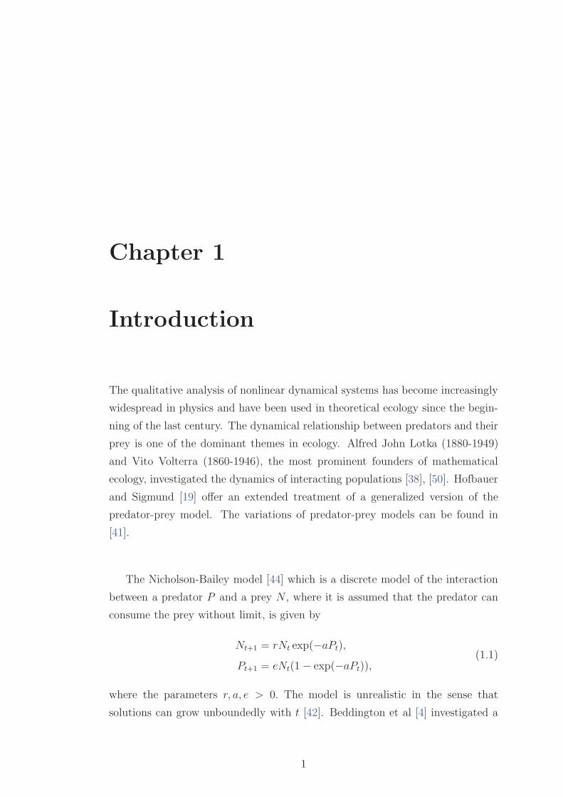
Chapter 1
Introduction
The qualitative analysis of nonlinear dynamical systems has become increasingly
widespread in physics and have been used in theoretical ecology since the begin-
ning of the last century. The dynamical relationship between predators and their
prey is one of the dominant themes in ecology. Alfred John Lotka (1880-1949)
and Vito Volterra (1860-1946), the most prominent founders of mathematical
ecology, investigated the dynamics of interacting populations [38], [50]. Hofbauer
and Sigmund [19] offer an extended treatment of a generalized version of the
predator-prey model. The variations of predator-prey models can be found in
[41].
The Nicholson-Bailey model [44] which is a discrete model of the interaction
between a predator P and a prey N , where it is assumed that the predator can
consume the prey without limit, is given by
Nt+1 = rNt exp(−aPt),
Pt+1 = eNt(1− exp(−aPt)),(1.1)
where the parameters r, a, e > 0. The model is unrealistic in the sense that
solutions can grow unboundedly with t [42]. Beddington et al [4] investigated a
1
CHAPTER 1. INTRODUCTION 2
density-dependent predator-prey model where the host rate of increase is logistic:
Nt+1 = Nt exp
[
r
(
1− Nt
K
)
− aPt
]
,
Pt+1 = eNt(1− exp(−aPt))
(1.2)
where K is the carrying capacity.
Hone, Irle, and Thurura [21] has studied the following predator-prey system
which is the more general form of the system (1.1):
Nt+1 = rNt exp(−aPt),
Pn+1 = eNt(1− exp(−bPt)).(1.3)
The main goal of this thesis is to investigate the following density-dependent
predator-prey model, which is the generalization of models (1.1), (1.2), and (1.3):
Nt+1 = Nt exp
[
r
(
1− Nt
K
)
− aPt
]
,
Pt+1 = eNt[1− exp(−bPt)],
(1.4)
where the parameters r,K, a, b, e are positive.
In this thesis, we also discuss the stability analysis of the Beddington model
with an Allee effect. The Allee effect is a phenomenon in biology characterized by
a positive correlation between population size or density and the mean individual
fitness of a population or species [1]. Although the concept of Allee effect had no
title at the time, it was first described in the 1930s by its namesake, Warder Clyde
Allee. Through experimental studies, Allee was able to demonstrate that goldfish
grow more rapidly when there are more individuals within the tank [1]. This led
him to conclude that aggregation can improve the survival rate of individuals,
and that cooperation may be crucial in the overall evolution of social structure.
The classical view of population dynamics stated that due to competition for
CHAPTER 1. INTRODUCTION 3
resources, a population will experience a reduced overall growth rate at higher
density and increased growth rate at lower density. In other words, we would be
better off when there are fewer of us around due to a limited amount of resources.
However, the Allee effect concept introduced the idea that the reverse holds true
when the population density is low. Individuals within a species generally require
the assistance of another for more than simple reproductive reasons in order to
persist. Examples of these can easily be seen in animals that hunt for prey or
defend against predators as a group.
This thesis is organized as follows: A review of the basic theory of discrete
dynamical systems and related population models are contained in Chapter 2. In
Chapter 3, the concept of Allee effect and an example of a predator-prey model
with Allee effect are presented. We investigate the stability analysis of the model.
The main problem, namely, the generalized Beddington model is given in Chapter
4. The stability and bifurcation for the problem is investigated and the numerical
computations are also confirm our results. We also discuss the stability analysis
of the Beddington model with an Allee effect. In the last chapter, we present the
final remarks and future work of our research.

Chapter 2
Preliminaries
2.1 Stability of Fixed Points for One-Dimesional
Maps
Most of the definitions and the theorems given in this chapter are taken directly
from [13], [35], [18], and [3].
Definition. Consider the difference equation
xn+1 = f(xn). (2.1)
A point x∗ is said to be a fixed point of the map f or an equilibrium point of
equation (2.1) if f(x∗) = x∗.
Closely related fixed points are the eventually fixed points. These are the
points that reach a fixed point after finitely many iterations. More explicitely,
a point x is said to be an eventually fixed point of a map f if there exist a
positive integer r and a fixed point x∗ of f such that f r(x) = x∗, but f r−1(x) 6= x∗,
where f r = f ◦ f ◦ f ◦ · · · f ◦ f︸ ︷︷ ︸
r compositions
.
The set of all fixed points is denoted by Fix(f), the set of all eventually fixed
4
CHAPTER 2. PRELIMINARIES 5
points by EFix(f), and the set of all eventually fixed points of the fixed point
x∗ by EFixx∗(f).
Theorem 2.1 Let f : I → I be a continuous map, where I = [a, b] is a closed
interval in R. Then, f has a fixed point.
Theorem 2.2 Let f : I → R be a continuous map such that f(I) ⊃ I. Then f
has a fixed point in I.
Definition. Let f : I → I be a map and x∗ ∈ I be a fixed point of f , where I is
an interval in the set of real numbers R. Then
1. x∗ is said to be stable if for any ε > 0 there exists δ > 0 such that for all
x ∈ I with |x− x∗| < δ we have |fn(x)− x∗| < ε for all n ∈ Z+. Otherwise,
the fixed point x∗ will be called unstable.
2. x∗ is said to be attracting if there exists η > 0 such that |x − x∗| < η
implies limn→∞
fn(x) = x∗.
3. x∗ is said to be asymptotically stable if it is both stable and attracting.
If in (2) η =∞, then x∗ is said to be globally asymptotically stable.
Fixed points may be divided into two types: hyperbolic and nonhyper-
bolic. A fixed point x∗ of a map f is said to be hyperbolic if |f(x∗)| 6= 1.
Otherwise, it is nonhyperbolic.
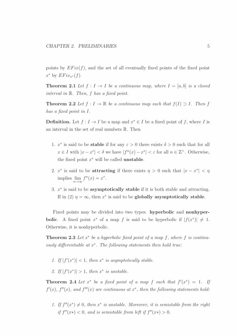
Theorem 2.3 Let x∗ be a hyperbolic fixed point of a map f , where f is continu-
ously differentiable at x∗. The following statements then hold true:
1. If |f ′(x∗)| < 1, then x∗ is asymptotically stable.
2. If |f ′(x∗)| > 1, then x∗ is unstable.
Theorem 2.4 Let x∗ be a fixed point of a map f such that f ′(x∗) = 1. If
f ′(x), f ′′(x), and f ′′′(x) are continuous at x∗, then the following statements hold:
1. If f ′′(x∗) 6= 0, then x∗ is unstable. Moreover, it is semistable from the right
if f ′′(x∗) < 0, and is semistable from left if f ′′(x∗) > 0.

CHAPTER 2. PRELIMINARIES 6
2. If f ′′(x∗) = 0 and f ′′′(x∗) > 0, then x∗ is unstable.
3. If f ′′(x∗) = 0 and f ′′′(x∗) < 0, then x∗ is asymptotically stable.
Definition. The Schwarzian derivative, Sf , of a function f is defined by
Sf(x) =f ′′′(x)
f ′(x)− 3
2
[f ′′(x)
f ′(x)
]2
.
And if f ′(x∗) = −1, then
Sf(x∗) = −f ′′′(x∗)− 3
2[f ′′(x∗)]2.
Theorem 2.5 Let x∗ be a fixed point of a map f such that f ′(x∗) = −1. If f ′(x),f ′′(x), and f ′′′(x) are continuous at x∗, then the following statements hold:
1. If Sf(x∗) < 0, then x∗ is asymptotically stable.
2. If Sf(x∗) > 0, then x∗ is unstable. Moreover, it cannot be semistable.
2.2 Stability of Fixed Points for Two-Dimensional
Maps
Definition. A fixed point X∗ of a map f : R2 → R2 is said to be
1. stable if given ε > 0 there exists δ > 0 such that |X − X∗| < δ implies
|fn(X)−X∗| < ε for all n ∈ Z+.
2. attracting (sink) if there exists ν > 0 such that |X − X∗| < ν implies
limn→∞ fn(X) = X∗. It is globally attracting if ν =∞.
3. asymptotically stable if it is both stable and attracting. It is globally
asymptotically stable if it is both stable and globally attracting.
CHAPTER 2. PRELIMINARIES 7
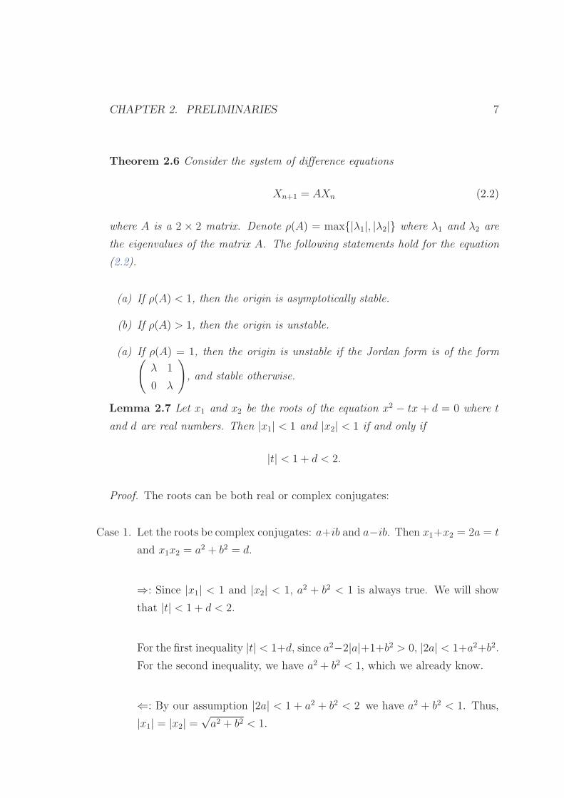
Theorem 2.6 Consider the system of difference equations
Xn+1 = AXn (2.2)
where A is a 2 × 2 matrix. Denote ρ(A) = max{|λ1|, |λ2|} where λ1 and λ2 are
the eigenvalues of the matrix A. The following statements hold for the equation
(2.2).
(a) If ρ(A) < 1, then the origin is asymptotically stable.
(b) If ρ(A) > 1, then the origin is unstable.
(a) If ρ(A) = 1, then the origin is unstable if the Jordan form is of the form(
λ 1
0 λ
)
, and stable otherwise.
Lemma 2.7 Let x1 and x2 be the roots of the equation x2 − tx + d = 0 where t
and d are real numbers. Then |x1| < 1 and |x2| < 1 if and only if
|t| < 1 + d < 2.
Proof. The roots can be both real or complex conjugates:
Case 1. Let the roots be complex conjugates: a+ib and a−ib. Then x1+x2 = 2a = t
and x1x2 = a2 + b2 = d.
⇒: Since |x1| < 1 and |x2| < 1, a2 + b2 < 1 is always true. We will show
that |t| < 1 + d < 2.
For the first inequality |t| < 1+d, since a2−2|a|+1+b2 > 0, |2a| < 1+a2+b2.
For the second inequality, we have a2 + b2 < 1, which we already know.
⇐: By our assumption |2a| < 1 + a2 + b2 < 2 we have a2 + b2 < 1. Thus,
|x1| = |x2| =√a2 + b2 < 1.
CHAPTER 2. PRELIMINARIES 8
Case 2. Now, let the roots be real.
⇒: Since |x1| < 1 and |x2| < 1, we have 0 < (1 − x1)(1 − x2) =
1 − x1 − x2 + x1x2 from which we get x1 + x2 < 1 + x1x2. Similarly,
using the fact that 0 < (1 + x1)(1 + x2), we get −(x1 + x2) < 1 + x1x2.
Combining these two inequalities, we obtain |x1 + x2| < 1 + x1x2. The
second part of the inequality is obvious.
⇐: We assume that |x1 + x2| < 1 + x1x2 and x1x2 < 1 which yields
−1 − x1x2 < x1 + x2 < 1 + x1x2
or
−(1 + x1)(1 + x2) < 0 < (1− x1)(1− x2).
Thus, we have
(1− x1)(1− x2) > 0,
(1 + x1)(1 + x2) > 0.
By the assumption, we also have that x1x2 < 1.
If |x1| ≥ 1 or/and |x2| ≥ 1, then at least one of the conditions above can
not be satisfied. Further, |x1| < 1 and |x2| < 1 satisfy the conditions above.
Hence, we have the following theorem:
Theorem 2.8 In equation (2.2), the origin is asymptotically stable if the follow-
ing condition holds true:
|trA| − 1 < detA < 1.
CHAPTER 2. PRELIMINARIES 9
In Appendix B, Table B.1, B.2, and B.3 represent some trace and determinant
values in the Trace-Determinant plane, their corresponding eigenvalues, and the
orbits of a linear system in the phase diagram. On the column Eigenvalues, two
dots represent the eigenvalues on the complex plane with the unit circle. The
phase diagram of the linear system with the corresponding eigenvalues is given
on the column Phase Plane. The black dot represents the final point after 100
iterations.
On the column Tr-Det Diagram, if the point is in the region given by the
Theorem 2.8, then the system is stable. Hence, the eigenvalues are inside the
unit circle and final point is at the origin. If the point is outside the region given
by the Theorem 2.8, then the system is unstable. So, the eigenvalues are outside
the unit circle and final point is far from the origin.
2.3 Invariant Manifolds
In this section, the appropriate tools that allows us to compute the center mani-
folds and the stable and unstable manifolds are presented [18], [13].
Let F : Rk → Rk be a map such that F ∈ C2 and F (0) = 0. Then one may
write F as a perturbation of a linear map L,
F (X) = LX +R(X)
where L is a k × k matrix defined by L = D(F (0)), R(0) = 0, and DR(0) = 0,
where D denotes the derivative. Now we will introduce special subspace of Rk,
called invariant manifolds [53].
An invariant manifold is a manifold embedded in its phase space with the
property that it is invariant under the dynamical system generated by F. A
subspace M of Rk is an invariant manifold if whenever X ∈M, then F n(X) ∈M,
CHAPTER 2. PRELIMINARIES 10
for all n ∈ Z+. For the linear map L, one may split its spectrum σ(L) into three
sets σs, σu, and σc, for which λ ∈ σs if |λ| < 1, λ ∈ σu if |λ| > 1, and λ ∈ σc if
|λ| = 1.
Corresponding to these sets, we have three invariant manifolds (linear sub-
spaces) Es, Eu, and Ec which are the generalized eigenspaces corresponding to
σs, σu, and σc, respectively.
The main question is how to extend this linear theory to nonlinear maps.
Corresponding to the linear subspaces Es, Eu, and Ec, we will have the invariant
manifolds the stable manifold W s, the unstable manifold W u, and the center
manifold W c.
The center manifolds theory is interesting only if W u = {0}. In this case, the
dynamics on the center manifold W c determines the dynamics of the system. The
other interesting case is when W c = {0} and we have a saddle. For the center
manifold theory we reference [6],[7],[32],[53],[40],[51].
Let Es ⊂ Rs, Eu ⊂ R
u, and Ec ⊂ Rt, with s + u + t = k. Then one may
formally define the above-mentioned invariant manifolds as follows:
W s = {x ∈ Rk : F n(x)→ 0 as n→∞},
W u = {x ∈ Rk : F n(x)→ 0 as n→ −∞}.
Since the stability on the center manifold is not a priori known, it is defined as a
manifold of dimension t whose graph is tangent to Ec at the origin.
Theorem 2.9 (Invariant Manifolds Theorem) [23],[40] Suppose that F ∈ C2.
Then there exist C2 stable W s and unstable W u manifolds tangent to Es and Eu,
respectively, at X = 0 and C1 center manifold W c tangent to Ec at X = 0.
Moreover, the manifolds W c, W s, and W u are all invariant.
CHAPTER 2. PRELIMINARIES 11
2.3.1 Center Manifolds
In this section, we focus on the case when σu = ∅. Hence the eigenvalues of L are
either inside the unit disc or on the unit disc. By suitable change of variables,
one may represent the map F as a system of difference equation such as
xn+1 = Axn + f(xn, yn),
yn+1 = Byn + g(xn, yn).(2.3)
First we assume that all eigenvalues of At×t are on the unit circle and all the
eigenvalues of Bs×s are inside the unit circle, with t+ s = k. Moreover,
f(0, 0) = 0, g(0, 0) = 0, Df(0, 0) = 0, Dg(0, 0) = 0.
Since W c is tangent to Ec = {(x, y) ∈ Rt×R
t : y = 0}, it may be represented
locally as the graph of a function h : Rt → Rt such that
W c = {(x, y) ∈ Rt×Rt : y = h(x), h(0) = 0, Dh(0) = 0, |x| < δ for a sufficently small δ}.
Furthermore, the dynamics restricted to W c is given locally by the equations
xn+1 = Axn + f(xn, h(xn)), x ∈ Rt. (2.4)
The main feature of equation (2.4) is that its dynamics determine the dynam-
ics of equation (2.3). So if x∗ = 0 is a stable, asymptotically stable, or unstable
fixed point of equation (2.4), then the fixed point (x∗, y∗) = (0, 0) of equation
(2.3) possesses the corresponding property.
To find the map y = h(x), we substitute for y in equation (2.3) and obtain
CHAPTER 2. PRELIMINARIES 12
� �� � � �� �
(a)
� � � �� �� �
(b)
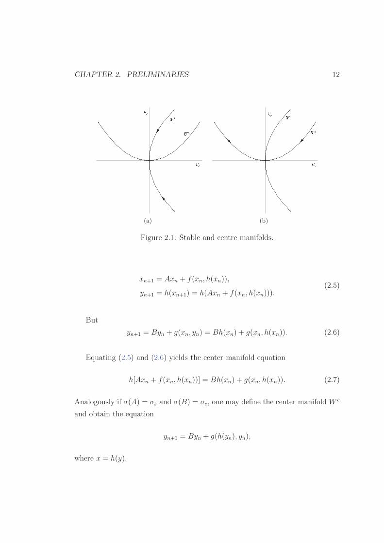
Figure 2.1: Stable and centre manifolds.
xn+1 = Axn + f(xn, h(xn)),
yn+1 = h(xn+1) = h(Axn + f(xn, h(xn))).(2.5)
But
yn+1 = Byn + g(xn, yn) = Bh(xn) + g(xn, h(xn)). (2.6)
Equating (2.5) and (2.6) yields the center manifold equation
h[Axn + f(xn, h(xn))] = Bh(xn) + g(xn, h(xn)). (2.7)
Analogously if σ(A) = σs and σ(B) = σc, one may define the center manifold W c
and obtain the equation
yn+1 = Byn + g(h(yn), yn),
where x = h(y).
CHAPTER 2. PRELIMINARIES 13
2.3.2 Stable and Unstable Manifolds
Suppose now that the map F is hyperbolic, that is σc = ∅. Then by Theorem 2.9,
there are two unique invariant manifolds W s and W u tangent to Es and Eu at
X = 0, which are graphs of the maps
ϕ1 : E1 → E2 and ϕ2 : E2 → E1,
such that
ϕ1(0) = ϕ2(0) = 0 and D(ϕ1(0)) = D(ϕ2(0)) = 0.
Letting yn = ϕ1(xn) yields
yn+1 = ϕ1(xn+1) = ϕ1(Axn + f(xn, ϕ1(xn))).
But
yn+1 = Bϕ1(xn) + g(xn, ϕ1(xn)).
Equating the two equations above yields
ϕ1(Axn + Cϕ1(xn) + f(xn, ϕ1(xn))) = Bϕ1(xn) + g(xn, ϕ(xn)), (2.8)
where we can take, without loss of generality,
ϕ1(x) = α1x2 + β1x
3 +O(|x|4).
Similarly, letting xn = ϕ2(yn) yields
xn+1 = ϕ2(yn+1) = ϕ2(Byn + g(ϕ2(yn), yn)), (2.9)
where we can take, without loss of generality,
ϕ2(x) = α2x+ β2x2 +O(|x|3).
But
xn+1 = Aϕ2(yn) + Cyn + f(ϕ2(yn), yn), (2.10)
CHAPTER 2. PRELIMINARIES 14
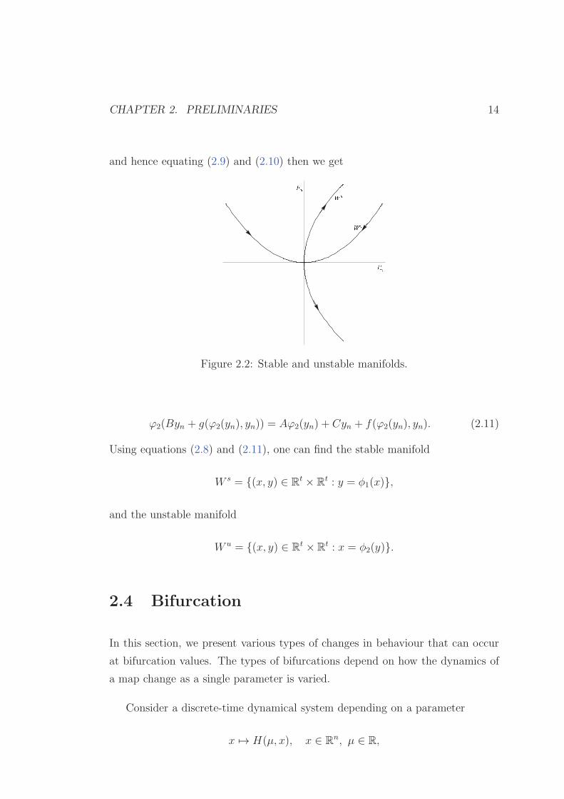
and hence equating (2.9) and (2.10) then we get
� �� � � �� �
Figure 2.2: Stable and unstable manifolds.
ϕ2(Byn + g(ϕ2(yn), yn)) = Aϕ2(yn) + Cyn + f(ϕ2(yn), yn). (2.11)
Using equations (2.8) and (2.11), one can find the stable manifold
W s = {(x, y) ∈ Rt × R
t : y = φ1(x)},
and the unstable manifold
W u = {(x, y) ∈ Rt × R
t : x = φ2(y)}.
2.4 Bifurcation
In this section, we present various types of changes in behaviour that can occur
at bifurcation values. The types of bifurcations depend on how the dynamics of
a map change as a single parameter is varied.
Consider a discrete-time dynamical system depending on a parameter
x 7→ H(µ, x), x ∈ Rn, µ ∈ R,
CHAPTER 2. PRELIMINARIES 15
where the map H is smooth with respect to both x and µ.
Let x = x0 be a hyperbolic fixed point of the system for µ = µ0. Let us monitor
this fixed point and its eigenvalues while this parameter varies. It is clear that
there are, generically, only three ways in which the hyperbolicity condition can
be violated. Either a simple positive eigenvalue approaches the unit circle and
we have λ1 = 1, or a simple negative eigenvalue approaches the unit circle and
we have λ1 = −1, or a pair of simple complex eigenvalues reach the unit circle
and we have λ1,2 = e±iθ0 , 0 < θ0 < π, for some value of parameter. Now, we give
the following definitions.
Definition. The bifurcation associated with the appearance of λ1 = 1 is called
a fold (or tangent) bifurcation.
This bifurcation is also referred to as a limit point, saddle-node bifurca-
tion, turning point, among others.
Definition. The bifurcation associated with the appearance of λ1 = −1 is called
a flip (or period doubling) bifurcation.
Definition. The bifurcation corresponding to the presence of λ1,2 = e±iθ0, 0 <
θ0 < π, is called a Neimark-Sacker (or torus) bifurcation [43], [46].
Notice that the fold and flip bifurcations are possible if n ≥ 1, but for the
Neimark-Sacker bifurcation we need n ≥ 2.
Theorem 2.10 (The Saddle-node Bifurcation) Suppose that Hµ(x) ≡H(µ, x) is a C2 one-parameter family of one-dimensional maps. (i.e., both∂2H∂x2 and ∂2H
∂µ2 exist and are continuous), and x∗ is a fixed point of Hµ∗ , with
H ′
µ∗(x∗) = 1. Assume further that
A =∂H
∂µ(µ∗, x∗) 6= 0 and B =
∂2H
∂x2(µ∗, x∗) 6= 0.
Then there exists an interval I around x∗ and a C2 map µ = p(x), where p : I → R
such that p(x∗) = µ∗, and Hp(x)(x) = x. Moreover, if AB < 0, the fixed points
exist for µ > µ∗, and if AB > 0, the fixed point exist for µ < µ∗.
CHAPTER 2. PRELIMINARIES 16
The proof of the above theorem can be found in [13]. For the proof, a version
of Implicit Function Theorem is used. We state the theorem below:
Theorem 2.11 (The Implicit Function Theorem) Suppose that G : R×R→R is a C1 map in both variables such that for some (µ∗, x∗) ∈ R×R, G(µ∗, x∗) = 0
and ∂G∂µ
(µ∗, x∗) 6= 0. Then, there exists an open interval J around µ∗, an open
interval I around x∗, and a C1 map µ = p(x), where p : I → J such that
1. p(x∗) = µ∗.
2. G(p(x), x) = 0, for all x ∈ I.
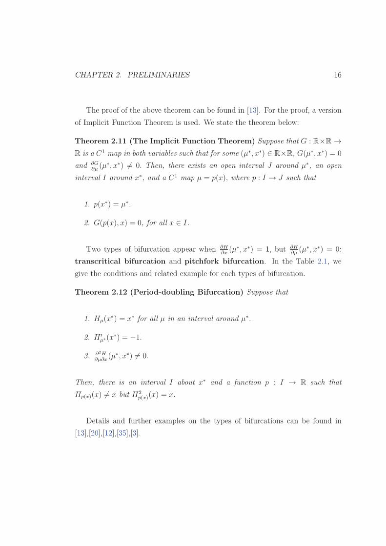
Two types of bifurcation appear when ∂H∂x
(µ∗, x∗) = 1, but ∂H∂µ
(µ∗, x∗) = 0:
transcritical bifurcation and pitchfork bifurcation. In the Table 2.1, we
give the conditions and related example for each types of bifurcation.
Theorem 2.12 (Period-doubling Bifurcation) Suppose that
1. Hµ(x∗) = x∗ for all µ in an interval around µ∗.
2. H ′
µ∗(x∗) = −1.
3. ∂2H∂µ∂x
(µ∗, x∗) 6= 0.
Then, there is an interval I about x∗ and a function p : I → R such that
Hp(x)(x) 6= x but H2p(x)(x) = x.
Details and further examples on the types of bifurcations can be found in
[13],[20],[12],[35],[3].
CHAPTER 2. PRELIMINARIES 17
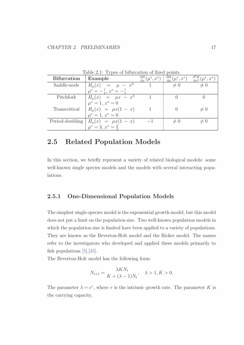
Table 2.1: Types of bifurcation of fixed points.
Bifurcation Example ∂H∂x
(µ∗, x∗) ∂H∂µ
(µ∗, x∗) ∂2H∂x2 (µ
∗, x∗)
Saddle-node Hµ(x) = µ − x2
µ∗ = −14, x∗ = −1
2
1 6= 0 6= 0
Pitchfork Hµ(x) = µx − x3
µ∗ = 1, x∗ = 01 0 0
Transcritical Hµ(x) = µx(1 − x)µ∗ = 1, x∗ = 0
1 0 6= 0
Period-doubling Hµ(x) = µx(1 − x)µ∗ = 3, x∗ = 2
3
−1 6= 0 6= 0
2.5 Related Population Models
In this section, we briefly represent a variety of related biological models: some
well-known single species models and the models with several interacting popu-
lations.
2.5.1 One-Dimensional Population Models
The simplest single-species model is the exponential growth model, but this model
does not put a limit on the population size. Two well-known population models in
which the population size is limited have been applied to a variety of populations.
They are known as the Beverton-Holt model and the Ricker model. The names
refer to the investigators who developed and applied these models primarily to
fish populations [5],[45].
The Beverton-Holt model has the following form:
Nt+1 =λKNt
K + (λ− 1)Nt
, λ > 1, K > 0.
The parameter λ = er, where r is the intrinsic growth rate. The parameter K is
the carrying capacity.
CHAPTER 2. PRELIMINARIES 18
The Ricker model has the following form:
Nt+1 = Nt exp
[
r
(
1− Nt
K
)]
,
where r > 0 is interpreted as intrinsic growth rate and K > 0 is the carrying
capacity.
This model is a limiting case of the Hassell model [16] which takes the form
Nt+1 =RNn
(1 + kNn)b,
where R, k > 0 and b > 1. When b = 1, the Hassel model is simply the Beverton-
Holt model.
2.5.2 Two-Dimensional Population Models
2.5.2.1 Nicholson-Bailey Model
One of the most well-known model for many experimental and theoretical in-
vestigations in ecology is Nicholson-Bailey host-parasitoid model [44]. This is a
discrete-time model to a biological system involved two insects, a parasitoid and
its host. Nicholson and Bailey developed the model (1935) and applied it to the
parasitiod (Encarsia formosa) and the host (Trialeurodes vaporariorum). The
term “parasitoid” means a parasite which is free living as an adult but lays eggs
in the larvae or pupae of the host. Hosts that are not parasitized give rise to their
own progeny. Hosts that are successfully parasitized die but the eggs laid by the
parasitoid may survive to be the next generation of parasitoids.
The general host-parasitoid model has the form
Nt+1 = rNtf(Nt, Pt), (2.12)
Pt+1 = eNt(1− f(Nt, Pt)), (2.13)
CHAPTER 2. PRELIMINARIES 19
where Nt is the density of host species in generation t, Pt is the density of para-
sitoid species in generation t, f(Nt, Pt) is the fraction of hosts not parasitized, r
is the number of eggs laid by a host that survive through the larvae, pupae, and
adult stages, and e is the number of eggs laid by a parasitoid on a single host
that survive through larvae, pupae, and adult stages. The parameter r and e are
positive.
The function f can be interpreted as the probability that each individual
host escapes the parasites, so that the complementary term 1 − f in the second
equation is the probability of being parasitized. Note that if Nt = 0, then Pt = 0
that is the parasitoid cannot survive without the host. That is why parasitoids
are good biological control agents.
Nicholson and Bailey model assumes a simple functional form for f(Nt, Pt). f
depends on the searching behavior of the parasitoid. The number encounters of
the parasitoids, Pt, with the hosts, Nt is in direct proportion to host density Nt,
that is, follows the law of mass action, aNtPt. The parameter a is the searching
efficiency of the parasitoid which is the probability that a given parasitoid will
encounter a given host during its searching lifetime. Since the number of encoun-
ters are distributed randomly among the available hosts, Nicholson and Bailey
used the Poisson distribution: p(n) = e−µµn
n!, where n is the number of encounters
and µ is the mean of encounters per host in one generation. Once the host is
parasitized, it will not be parasitized again. Host with no encounters, p(0), are
separated from those with more than one encounter, 1 − p(0). The probability
of encounters of the host by parasitoid represents the fraction of hosts that are
not parasitized, that is, p(0) = e−µµ0
0!= eµ, where µ = encounters
Nt= aPt, thus
p(0) = f(Nt, Pt) = exp(−aPt):
Nt+1 = rNt exp(−aPt),
Pt+1 = eNt(1− exp(−aPt)).(2.14)
CHAPTER 2. PRELIMINARIES 20
2.5.2.2 Beddington Model
The following density-dependent predator-prey model was investigated by Bed-
dington et al [4]:
Nt+1 = Nt exp
[
r
(
1− Nt
K
)
− aPt
]
,
Pt+1 = eNt[1− exp(−aPt)],
(2.15)
where K is the carrying capacity and represents maximum population size that
can be supported due to availability of all the potentially limiting resources.
Note that model (2.14) reduces to the density independent one-species model
Nt+1 = rNt if the parasitoid is not present. Since this is not realistic for most of
the species, model (2.15) rectifies this situation by adopting the density-depending
Ricker model Nt+1 = Nt exp[r(1− Nt
K)], where K is the carrying capacity of the
host and is the sustainable size of the host. Moreover, in the absence of the para-
sitiod, the equilibrium K is globally asymptotically stable for 0 < r < 2 on (0,∞)
[13]. It is assumed that the parameters a, r, e,K are all positive real numbers.
2.5.2.3 The Host-Parasitoid Model Discussed in [21]
Hone, Irle, and Thurura [21] has studied the following predator-prey system which
is the more general form of the Nicholson-Bailey model, system (2.14):
Nt+1 = rNt exp(−aPt),
Pt+1 = eNt(1− exp(−bPt)).(2.16)
For the special case a = b, the dynamics is uninteresting in the sense that
either the two species can both die out, or the solutions can grow without bound.
However, in general, the model displays the more biologically relevant possibilities
that the two populations can asymptotically approach positive steady-state values
or move towards an attracting invariant curve in the phase plane. The latter
CHAPTER 2. PRELIMINARIES 21
scenario arises from a Neimark-Sacker bifurcation [43], [46] that takes place in
the (r, a) parameter space [21].
2.5.2.4 Generalized Beddington Model
In this thesis, we consider the following density-dependent predator-prey model
which is the generalization of models (2.14), (2.15), and (2.16). In [21], the
authors introduced the model as an open problem.
Nt+1 = Nt exp
[
r
(
1− Nt
K
)
− aPt
]
,
Pt+1 = eNt[1− exp(−bPt)],
(2.17)
where the parameters r,K, a, b, e are positive.
Notice that in equation (2.17), when a = b this is the Beddington model. With
unlimited capacity, for which the term Nt
Kvanishes, equation (2.17) becomes the
model discussed by Hone, et al. Further, if a = b and the capacity is unlimited,
we have Nicholson-Bailey model.
2.5.2.5 An Example of Stability Analysis of a Predator-prey Model
[49]
In equation (2.12), the growth factor is rN. In Hassell’s model [27], the growth
factor is of the formR
(1 + kHt)b,
where a, b > 0 and H is the host species. Hassell et al. [27] collected R- and
b-values for about two dozen species from field and laboratory observations, and
noted that the majority of these cases were within the stable region.
In this section, we study the stability analysis of the following host-parasite
model which is studied by Misra and Mitra [29] where the growing host is infected

CHAPTER 2. PRELIMINARIES 22
with the parasite:
Ht+1 =RHt
(1 +Ht)be−cPt
Pt+1 = Ht(1− e−cPt).
(2.18)
Note that such simplifications, including the convention k = 1 in the Hassell
model, lead to the interpretation of the “population” variable as a “suitable mul-
tiple of the population”.
Fixed Points of System (2.18)
In order to find the fixed points (H∗, P ∗) of system (2.18), we setHt = Ht+1 = H∗
and Pt = Pt+1 = P ∗:
H∗ =RH∗
(1 +H∗)be−cP
∗
,
P ∗ = H∗(1− e−cP∗
).
(2.19)
We first observe that for H∗ = 0, we have the extinction fixed point (0, 0)
for any values of parameters. For H∗ 6= 0 and P ∗ = 0, we obtain the solution
(R1b −1, 0). For H∗ 6= 0 and P ∗ 6= 0, from the first equation of the system (2.19),
we have
P ∗ =1
cln
[R
(1 +H∗)b
]
. (2.20)
Now, we can see that the parameter R is important for the existence of the fixed
points other than the extinction fix point (0,0). We have the following cases:
Case 1. R ≤ 1
For this case, we have R1b − 1 ≤ 0 and 1
cln[
R(1+H∗)b
]
< 0. Hence, there is no
exclusion and coexistence fixed point for R ≤ 1.
CHAPTER 2. PRELIMINARIES 23
Case 2. R > 1
In the first equation of the system (2.19), assuming that H∗ 6= 0, we have
e−cP∗
=(1 +H∗)b
R. (2.21)
Combining the equation (2.21) and the second equation of the system (2.19),
we obtain
P ∗ = H∗
(
1− (1 +H∗)b
R
)
.
Now, we can write the first equation of the system (2.18) as
H∗ =RH∗
(1 +H∗)be−cH∗
(
1− (1+H∗)b
R
)
,
or
(1 +H∗)b ecH∗−
cRH∗(1+H∗)b = R, (2.22)
an equation in the variable H∗. Let us denote
z = F (x) = (1 + x)b ecx−cRx(1+x)b .
When the graph of F intersects the horizontal line z = R, some fixed points are
obtained. Note that x = R1b − 1 is a solution of the equation F (x) = R, which
corresponds to the fixed point (R1b−1, 0) of the system (2.18). We will investigate
if there exist some other intersection points.
Setting F ′(x) = 0, we obtain the equation
R(b+ c+ cx)
c(1 + x+ bx)= (1 + x)b.
For x ≥ 0, the function on the right-hand side has y-intercept 1, and is mono-
tonically increasing without bound. On the other hand, the function on the
left-hand side is monotonically decreasing, has y-intercept R(1 + b/c) > 1, and
CHAPTER 2. PRELIMINARIES 24
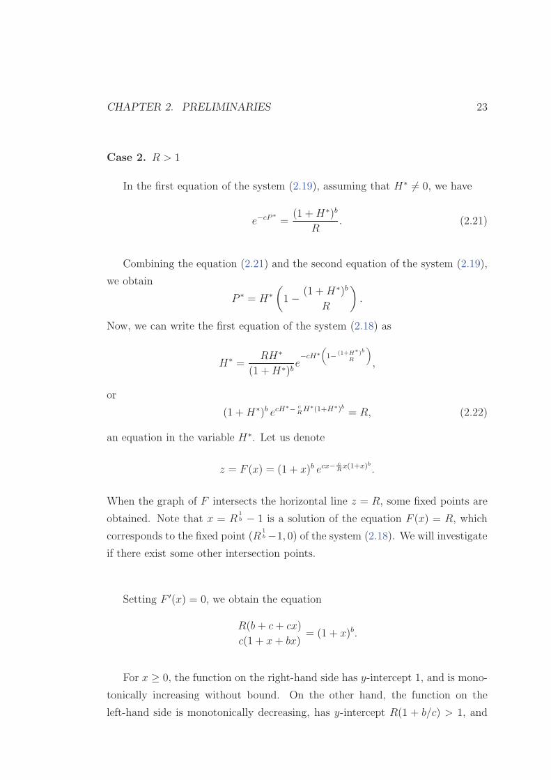
converges to R/(1 + b) as x → ∞. Thus, there is a unique intersection point
which means there exists only one critical point. See Figure 2.3.
� � � � � � � � � � � � � � � �����
Figure 2.3: y = R(b+c+cx)c(1+x+bx)
and y = (1 + x)b.
The intersection point is the point where F ′(x) = 0.
Since F (0) = 1, F ′(0) = c(R−1)+bR
R> 0, and F (x)→ 0 as x→∞, the critical
point is a local maximum. See Figure 2.4.
In Figure 2.4, we know that one of the intersection points is the solution
x = R1b −1. The other intersection point, say H , may or may not be a component
of a positive fixed point. In order to guarantee that P component is also positive,
we solve P ∗ > 0 in the equation (2.20) and obtain
H∗ < R1b − 1.
Thus, there exists a positive fixed point if F ′(R1b −1) < 0. Solving this inequality,
we obtain the condition for the existence of the positive fixed point: R >(
1 + 1c
)b.
Thus, we obtain the following result.
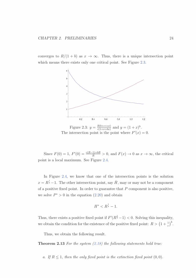
Theorem 2.13 For the system (2.18) the following statements hold true:
a. If R ≤ 1, then the only fixed point is the extinction fixed point (0, 0).
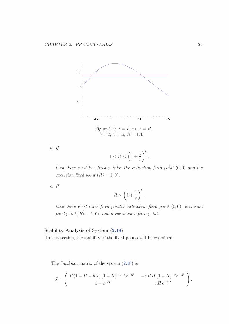
CHAPTER 2. PRELIMINARIES 25
� � � � � � � � � � � � � � �� � � � �� � Figure 2.4: z = F (x), z = R.
b = 2, c = .6, R = 1.4.
b. If
1 < R ≤(
1 +1
c
)b
,
then there exist two fixed points: the extinction fixed point (0, 0) and the
exclusion fixed point (R1b − 1, 0).
c. If
R >
(
1 +1
c
)b
,
then there exist three fixed points: extinction fixed point (0, 0), exclusion
fixed point (R1b − 1, 0), and a coexistence fixed point.
Stability Analysis of System (2.18)
In this section, the stability of the fixed points will be examined.
The Jacobian matrix of the system (2.18) is
J =
(
R (1 +H − bH) (1 +H)−1−b e−cP −cRH (1 +H)−be−cP
1− e−cP cH e−cP
)
.
CHAPTER 2. PRELIMINARIES 26
At (0, 0), the Jacobian becomes
J0 =
(
R 0
0 0
)
.
The eigenvalues for the fixed point (0, 0) are λ1 = R and λ2 = 0. Hence, (0, 0) is
asymptotically stable if R < 1. We will now consider the exclusion fixed point.
Theorem 2.14 For the system (2.18), the exclusion fixed point (R1b − 1, 0) is
asymptotically stable if
max
(
c
c+ 1,b− 2
b
)
< R−1b < 1.
Proof. The Jacobian matrix evaluated at this point is given by
J2 =
1 + b(
−1 +R−1b
)
−c(
−1 +R1b
)
0 c(
−1 +R1b
)
,
where the eigenvalues are λ1 = 1+b(
−1 +R−1b
)
and λ2 = c(
−1 +R1b
)
. Apply-
ing the stability conditions |λ1| < 1 and |λ2| < 1, we obtain the desired result.
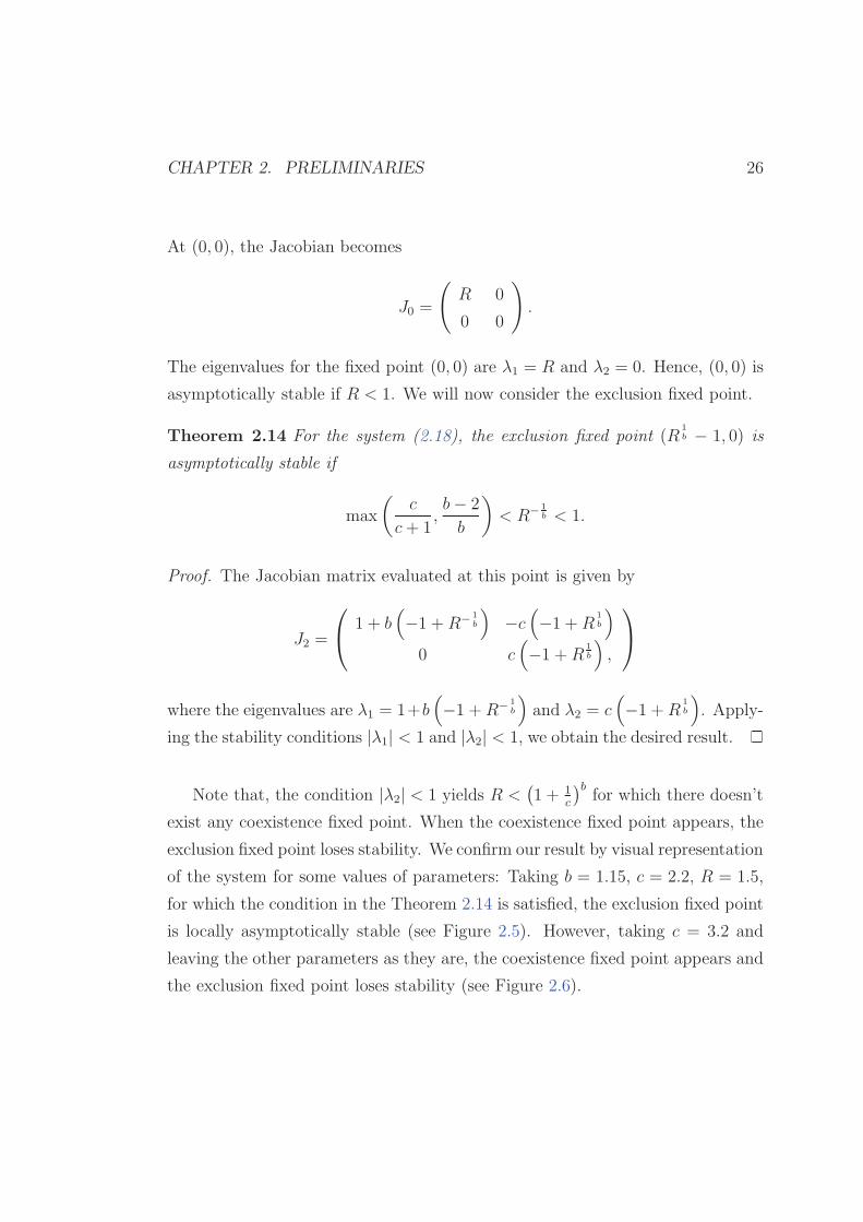
Note that, the condition |λ2| < 1 yields R <(
1 + 1c
)bfor which there doesn’t
exist any coexistence fixed point. When the coexistence fixed point appears, the
exclusion fixed point loses stability. We confirm our result by visual representation
of the system for some values of parameters: Taking b = 1.15, c = 2.2, R = 1.5,
for which the condition in the Theorem 2.14 is satisfied, the exclusion fixed point
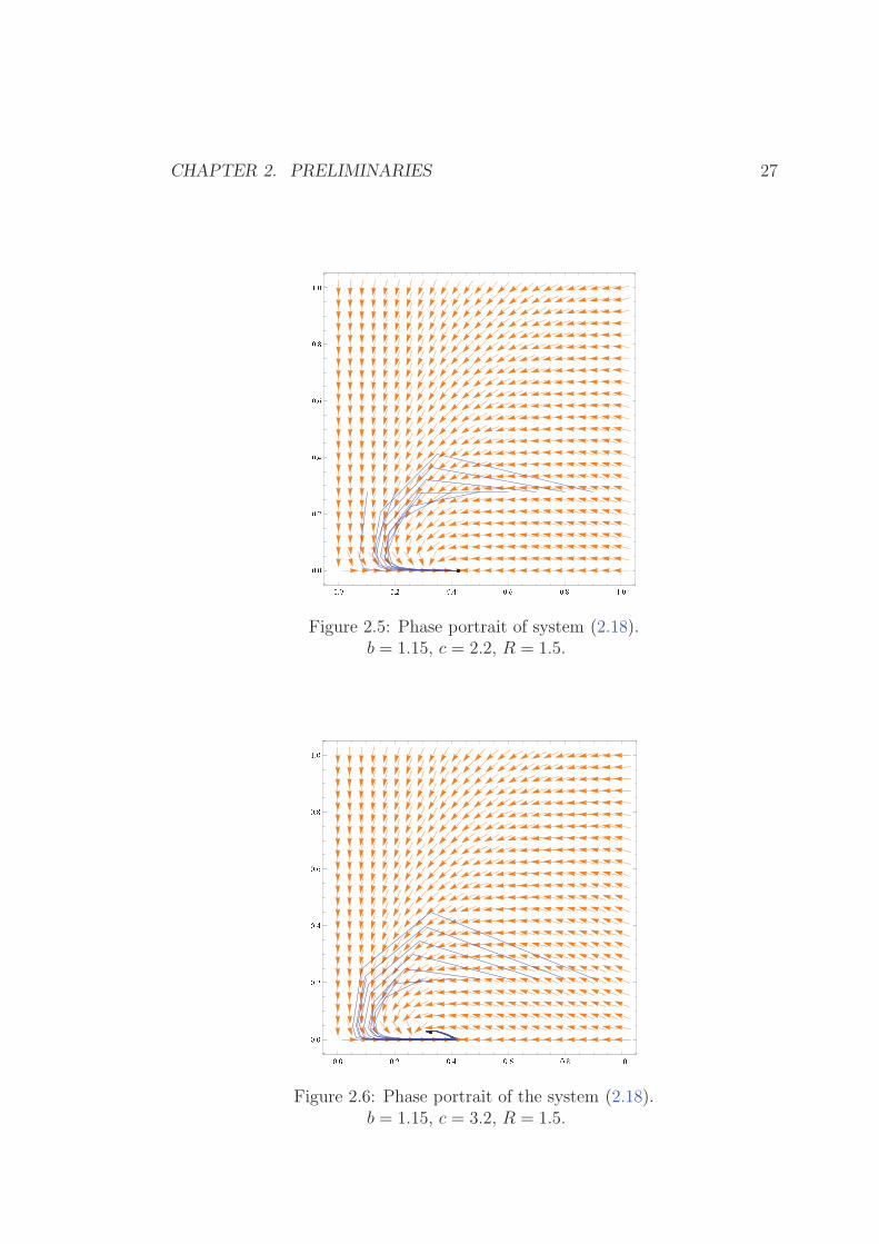
is locally asymptotically stable (see Figure 2.5). However, taking c = 3.2 and
leaving the other parameters as they are, the coexistence fixed point appears and
the exclusion fixed point loses stability (see Figure 2.6).
CHAPTER 2. PRELIMINARIES 27
� � � � � � � � � � � � � � � � � �� � �� � �� � �� � �� � �� � �
Figure 2.5: Phase portrait of system (2.18).b = 1.15, c = 2.2, R = 1.5.
� � � � � � � � � � � � � � � � � �� � �� � �� � �� � �� � �� � �
Figure 2.6: Phase portrait of the system (2.18).b = 1.15, c = 3.2, R = 1.5.
Chapter 3
Population Models with Allee
Effect
3.1 Allee Effect
Ecologist W.C. Allee (1931) was one of the first to write extensively on the ecolog-
ical significance of animal aggregation; hence, the positive relationship between
population density and the individual’s fitness is often known as “Allee Effect”.
This effect can be caused by difficulties in, for example, mate finding, social dys-
function, inbreeding depression, food exploitation (e.g., host resistance can only
be overcome by sufficient numbers of consumers), and predator avoidance or de-
fense [1].
The most important distinction within the Allee effect domain is between
component and demographic Allee effects. Component Allee effects are at the
level of components of individual fitness, for example juvenile survival or litter
size. Conversely, demographic Allee effects are at the level of the overall mean in-
dividual fitness, practically always viewed through the demography of the whole
population as the per capita population growth rate [9]. The two are related in
that component Allee effects may result in demographic Allee effects.
28
CHAPTER 3. POPULATION MODELS WITH ALLEE EFFECT 29
Allee proposed that the per capita birth rate declines at low population densi-
ties. Under such scenario, a population at low densities may slide into extinction.
Allee found that the highest per capita growth rates of the population of the flour
beetles, Tribolium cofusum, were at intermediate densities. Moreover, when fewer
mates were available, the females produced fewer eggs, a rather unexpected out-
come. Allee did not provide a definite and precise definition of this new notion.
Stephens, Sutherland, and Freckleton [24] defined the Allee effect as “a positive
relationship between any component of individual fitness and either numbers or
density of conspecifics.” In classical dynamics, we have a negative density depen-
dence, that is, fitness decreases with increasing density. The Allee effect, however,
produces a positive density dependence, that is, fitness increases with increasing
density [14].
The instability of the lower equilibrium (Allee threshold) [9] means that nat-
ural populations subject to a demographic Allee effect are unlikely to persist in
the range of population sizes where the effect is manifest. Another issue that may
cause some confusion in the use of the term Allee effect whether the phenomenon
is caused by low population sizes or by low population densities. Though for
field ecologists, a drop in number will be inseparable from a corresponding reduc-
tion in density. Allee himself considered both types of Allee effect and observed
the Allee effect caused by reduction in the number of mice, and the Allee effect
caused by the reduction in density of our beetles, Tribolium confusum [2]. In [25],
Stephens and Sutherland described several scenarios that cause the Allee effect in
both animals and plants. For example, cod and many freshwater fish species have
high juvenile mortality when there are fewer adults. While fewer red sea urchin
give rise to worsening feeding conditions of their young and less protection from
predation. In some mast flowering trees, such as Spartina alterniflora, with a low
density have a lower probability of pollen grain finding stigma in wind-pollinated
plants.

CHAPTER 3. POPULATION MODELS WITH ALLEE EFFECT 30
Any function f whose graph passes through the origin and remains below the
diagonal near zero and later crosses the diagonal twice will give rise to the Allee
effect [14].
As an example of modelling the Allee effect, consider the single-species pop-
ulation model
xn+1 = xner−xn, x0 > 0 (3.1)
where parameter r is positive. Model (3.1) with an Allee effect can be considered
to be
xn+1 = xner−xn
xn
m+ xn
, x0 > 0. (3.2)
The expression xn
m+xndenotes the probability of an individual successfully finding
a mate to reproduce or a cooperative individual to exploit resources, where pa-
rameter m > 0 is Allee constant [22].
3.2 A Predator-prey Model with Allee Effect
Now, we present an example of a predator-prey model with Allee effect and anal-
yse the stability of fixed points for the model.
The following discrete-time predator-prey system was studied by Celik and
Duman [10] with an Allee effect on the prey population and by Wang, Zhang,
and Liu [52] with Allee effects both on prey and predator:
Nt+1 = Nt + rNt(1−Nt)− aNtPt,
Pt+1 = Pt + aPt(Nt − Pt),(3.3)
where the parameters a, r are positive, Nt is prey density at time t and Pt is
predator density at time t, r is the intrinsic growth rate. The term aNt is per
capita predator increase due to prey consumption.
CHAPTER 3. POPULATION MODELS WITH ALLEE EFFECT 31
Now, we consider the system (3.3) when the predator population is subject
to an Allee effect which is more general form of the system (3.1) in [52].
Nt+1 = Nt + rNt(1−Nt)− aNtPt,
Pt+1 = Pt + aPt(Nt − Pt)P dt
m+ P dt
,(3.4)
where the parameters a, r,m are positive and d ≥ 1.
When d = 1, the system is the model with Allee effect on predator discussed
by Wang, Zhang, and Liu [52]. We will investigate the stability of fixed points for
the model (3.4) and analyse the stability of exclusion fixed point, which is non-
hyperbolic, for the particular cases when d = 1 and d = 2 by using the Center
Manifold Theory.
3.2.1 Stability of Fixed Points for System (3.4)
The fixed points are (0, 0), (1, 0), and ( ra+r
, ra+r
). The Jacobian matrix of the
planar map in (3.4) is
J =
1 + r − 2rN − aP −aNaP 1+d
m+P d
m2+(1+a(N−2P ))P 2d−mP d(−2−a((1+d)N−(2+d)P ))
(m+P d)2
.
The Jacobian matrix for the extinction fixed point (0, 0) is
J0 =
(
1 + r 0
0 1
)
.
CHAPTER 3. POPULATION MODELS WITH ALLEE EFFECT 32
(0,0) is unstable fixed point since one of the eigenvalues λ1 and λ2 is greater than
1. The Jacobian for the exclusion fixed point (1, 0) is
J1 =
(
1− r −a0 1
)
.
Since one of the eigenvalues of the matrix J1 is 1, this point is non-hyperbolic.
By using the Center manifold theory, we will show for some particular cases, in
the next section that this point is unstable.
Now, let us discuss the coexistence fixed point ( ra+r
, ra+r
): Jacobian matrix for
this point is
J∗ =
a+r−r2
a+r− ar
a+r
a( ra+r)
1+d
m+( ra+r)
d 1− a( ra+r)
1+d
m+( ra+r)
d
.
By using the Trace-Determinant formula, after some computation we obtain the
following result:
Theorem 3.1 The positive fixed point ( ra+r
, ra+r
) is asymptotically stable if
0 < r[(K +m)r + a(K −Kr)] < 4a(K +m)− aKr − (K +m)(−4 + r)r
where K =(
ra+r
)d.
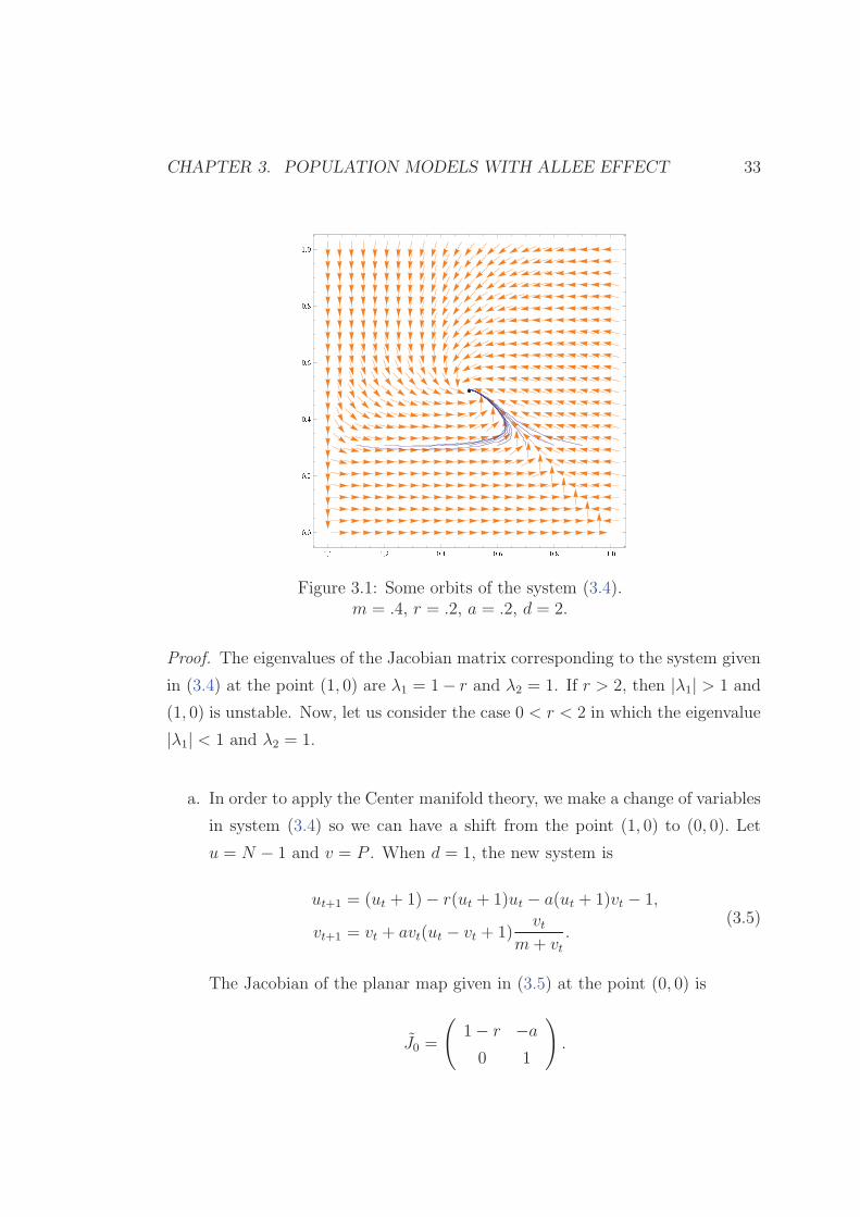
In Figure 3.1, we give the numerical evidence for some particular values of the
parameters that the positive fixed point is asymptotically stable.
3.2.2 Instability of Exclusion Fixed Point
In this section, by using the Center manifold theory, we show for some values of
d for the system (3.4), the fixed point (1, 0) is unstable.
Theorem 3.2 For the system (3.4), the following statements hold true:
a. If d = 1, then (1, 0) is unstable.
b. If d = 2, then (1, 0) is unstable.
CHAPTER 3. POPULATION MODELS WITH ALLEE EFFECT 33
� � � � � � � � � � � � � � � � � �� � �� � �� � �� � �� � �� � �
Figure 3.1: Some orbits of the system (3.4).m = .4, r = .2, a = .2, d = 2.
Proof. The eigenvalues of the Jacobian matrix corresponding to the system given
in (3.4) at the point (1, 0) are λ1 = 1− r and λ2 = 1. If r > 2, then |λ1| > 1 and
(1, 0) is unstable. Now, let us consider the case 0 < r < 2 in which the eigenvalue
|λ1| < 1 and λ2 = 1.
a. In order to apply the Center manifold theory, we make a change of variables
in system (3.4) so we can have a shift from the point (1, 0) to (0, 0). Let
u = N − 1 and v = P . When d = 1, the new system is
ut+1 = (ut + 1)− r(ut + 1)ut − a(ut + 1)vt − 1,
vt+1 = vt + avt(ut − vt + 1)vt
m+ vt.
(3.5)
The Jacobian of the planar map given in (3.5) at the point (0, 0) is
J0 =
(
1− r −a0 1
)
.
CHAPTER 3. POPULATION MODELS WITH ALLEE EFFECT 34
Now we can rewrite the equations in system (3.5) as
ut+1 = (1− r)ut − avt + f(ut, vt),
vt+1 = vt + g(ut, vt),(3.6)
where
f(ut, vt) = −ut(rut + avt)
and
g(ut, vt) =a(1 + ut − vt)v
2t
m+ vt.
Since invariant manifold is tangent to the corresponding eigenspace by The-
orem 2.9, we assume that the map h takes the form
h(u) = −r
au+ αu2 + βu3 +O(u4), α, β ∈ R.
Now we can compute the constants α and β. The function h must satisfy
the center manifold equation
h(
(1− r)u− ah(u) + f(u, h(u)))
− h(u)− g(u, h(u)) = 0.
By using the Taylor series expansion we can solve the functional equation
above: we obtain
αr − r2
ma= 0
and
αr + βr +2αr
m− r2
ma− r3
m2a2− r3
ma2− 2α
(
r + a(
α− r
a
))
= 0.
By solving the system we get α = rma
, β = r2+mr2
m2a2. Hence
h(u) = −r
au+
r
mau2 +
r2 +mr2
m2a2u3.
Thus on the center manifold v = h(u) we have the following map
S(u) = −u ((1 +m)r2u2(1 + u) +ma(−m+ ru(1 + u)))
m2a.
CHAPTER 3. POPULATION MODELS WITH ALLEE EFFECT 35
Since S ′(0) = 1 and S ′′(0) = −2rm
< 0. Hence, in that case the exclusion
fixed point (1, 0) is unstable.
b. Similarly, when d = 2, the new system is given by
ut+1 = (ut + 1)− r(ut + 1)ut − a(ut + 1)vt − 1,
vt+1 = vt + avt(ut − vt + 1)v2t
m+ v2t.
(3.7)
The Jacobian of the planar map which is given in (3.7) at the point (0, 0)
is
J0 =
(
1− r −a0 1
)
.
Now we can write the equations in system (3.7) as
ut+1 = (1− r)ut − avt + f(ut, vt),
vt+1 = vt + g(ut, vt),(3.8)
where
f(ut, vt) = −ut(rut + avt)
and
g(ut, vt) =a(1 + ut − vt)v
3t
m+ v2t.
Since invariant manifold is tangent to the corresponding eigenspace by The-
orem 2.9, let us assume that the map h takes the form
h(u) = −r
au+ αu2 + βu3 +O(u4), α, β ∈ R.
Now we can compute the constants α and β. The function h must satisfy
the center manifold equation
h(
(1− r)u− ah(u) + f(u, h(u)))
− h(u)− g(u, h(u)) = 0.
By using the Taylor series expansion we can solve the functional equation
above: we obtain
αr = 0

CHAPTER 3. POPULATION MODELS WITH ALLEE EFFECT 36
and
−2aα2 + (α + β)r +r3
ma2= 0
By solving the system we get α = 0, β = − r2
ma2. Hence
h(u) = −r
au− r2
ma2u3.
Thus on the center manifold v = h(u) we have the following map
R(u) =mau+ r2u3(1 + u)
ma.
Since R′(0) = 1 and R′′(0) = 0, we need the calculate the Schwarzian
derivative [13] at the origin: The Schwarzian derivative is 6r2
ma> 0 thus the
exclusion fixed point (1, 0) is unstable.
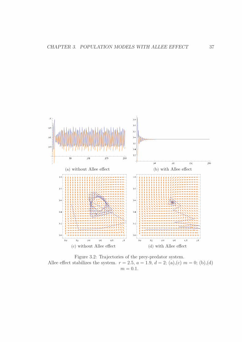
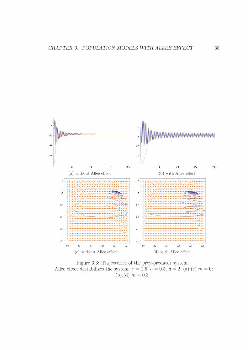
We show the influence of Allee effect on the local stability of fixed points for
system (3.4). In Figure 3.2 and Figure 3.3, we show the trajectories of predator-
prey densities in the system we studied. Figure 3.2 presents that the correspond-
ing equilibrium points can move from instability to stability under Allee effect.
On the other hand, Allee effect may be a destabilizing force in the predator-prey
system which made the equilibrium point change from stable to unstable. Fig-
ure 3.3 presents this fact. Table 3.1 also gives a compact information about the
stabilizing and destabilizing of Allee effect in the model.
Table 3.1: Allee effect may stabilize or destabilize the system.Figure r a d m Fixed Point Initial Point3.2(a), 3.2(c) 2.5 1.9 2 0 Unstable (0.3,0.2)3.2(b), 3.2(d) 2.5 1.9 2 0.1 Stable (0.3,0.2)3.3(a), 3.3(c) 2.5 0.5 2 0 Stable (0.3,0.2)3.3(b), 3.3(d) 2.5 0.5 2 0.3 Unstable (0.3,0.2)
CHAPTER 3. POPULATION MODELS WITH ALLEE EFFECT 37
� � � � � � � � � � �� !� "� #� �(a) without Allee effect
� � � � � � � � � � �� $� !� �� "� %� #� &(b) with Allee effect
� � � � � ! � " � # � �� �� �� !� "� #� �
(c) without Allee effect
� � � � � ! � " � # � �� �� �� !� "� #� �
(d) with Allee effect
Figure 3.2: Trajectories of the prey-predator system.Allee effect stabilizes the system. r = 2.5, a = 1.9, d = 2; (a),(c) m = 0; (b),(d)
m = 0.1.
CHAPTER 3. POPULATION MODELS WITH ALLEE EFFECT 38
� � � � � � � � � � �� !� "� #� �(a) without Allee effect
� � � � � � � � � � �� !� "� #� �(b) with Allee effect
� � � � � ! � " � # � �� �� �� !� "� #� �
(c) without Allee effect
� � � � � ! � " � # � �� �� �� !� "� #� �
(d) with Allee effect
Figure 3.3: Trajectories of the prey-predator system.Allee effect destabilizes the system. r = 2.5, a = 0.5, d = 2; (a),(c) m = 0;
(b),(d) m = 0.3.

CHAPTER 3. POPULATION MODELS WITH ALLEE EFFECT 39
For more details on Allee effect, see [1],[34],[36]. Many variants of predator-
prey models with Allee effect subject to predator and/or prey can be found in
[9],[14],[37].
Chapter 4
Main Problem
4.1 Generalized Beddington Model
We consider the following density-dependent predator-prey model which is a gen-
eralized version of the discrete systems (2.14), (2.15), and (2.16). In [21], the
authors introduced the model as an open problem.
Nt+1 = Nt exp
[
r
(
1− Nt
K
)
− aPt
]
,
Pt+1 = eNt[1− exp(−bPt)],
(4.1)
where the parameters a, b, e,K, and r are positive.
Notice that in equation (4.1), when a = b we obtain the Beddington model.
With unlimited capacity, for which the term Nt
Kvanishes, equation (4.1) becomes
the model discussed by Hone, et al. Further, if a = b and the capacity is unlim-
ited, we have Nicholson-Bailey model.
Now, we eliminate some of the parameters by changing the variables. Taking
40

CHAPTER 4. MAIN PROBLEM 41
xt =Nt
K, and yt = bPt, we obtain
xt+1 = xt exp [r (1− xt)− qyt] ,
yt+1 = µxt[1− exp(−yt)],(4.2)
where µ = beK and q = ab.
All the procedures we maintain for the case a 6= b in this thesis can be done
for the case a = b by taking q = 1.
4.1.1 Fixed Points
The fixed points of the discrete system (4.2) are obtained:
Theorem 4.1 For the system given in (4.2),
a. if µ ≤ 1, then there exist two non-negative fixed points which are (0, 0) and
(1, 0).
b. if µ > 1, there exist three fixed points which are (0, 0), (1, 0) and (`, rq(1−`))
where 0 < ` < 1. In this case, (`, rq(1 − `)) is coexistence (positive) fixed
point.
Proof. To find the fixed points of the system given in (4.2), the following system
of equations must be solved:
x = x exp [r (1− x)− qy] ,
y = µx[1− exp(−y)].(4.3)
If x = 0, we have the extinction fixed point (0, 0) and if x 6= 0, the system of
CHAPTER 4. MAIN PROBLEM 42
' ( ) * ( ' * ( ) + ( '-
' ( +-' ( *' ( *' ( +' ( ,' ( -
(a) µ = 1
' ( ) * ( ' * ( ) + ( '' ( )* ( '* ( )+ ( '(b) µ < 1
' ( ) * ( ' * ( ) + ( '-
' ( --' ( +' ( +' ( -
(c) µ > 1
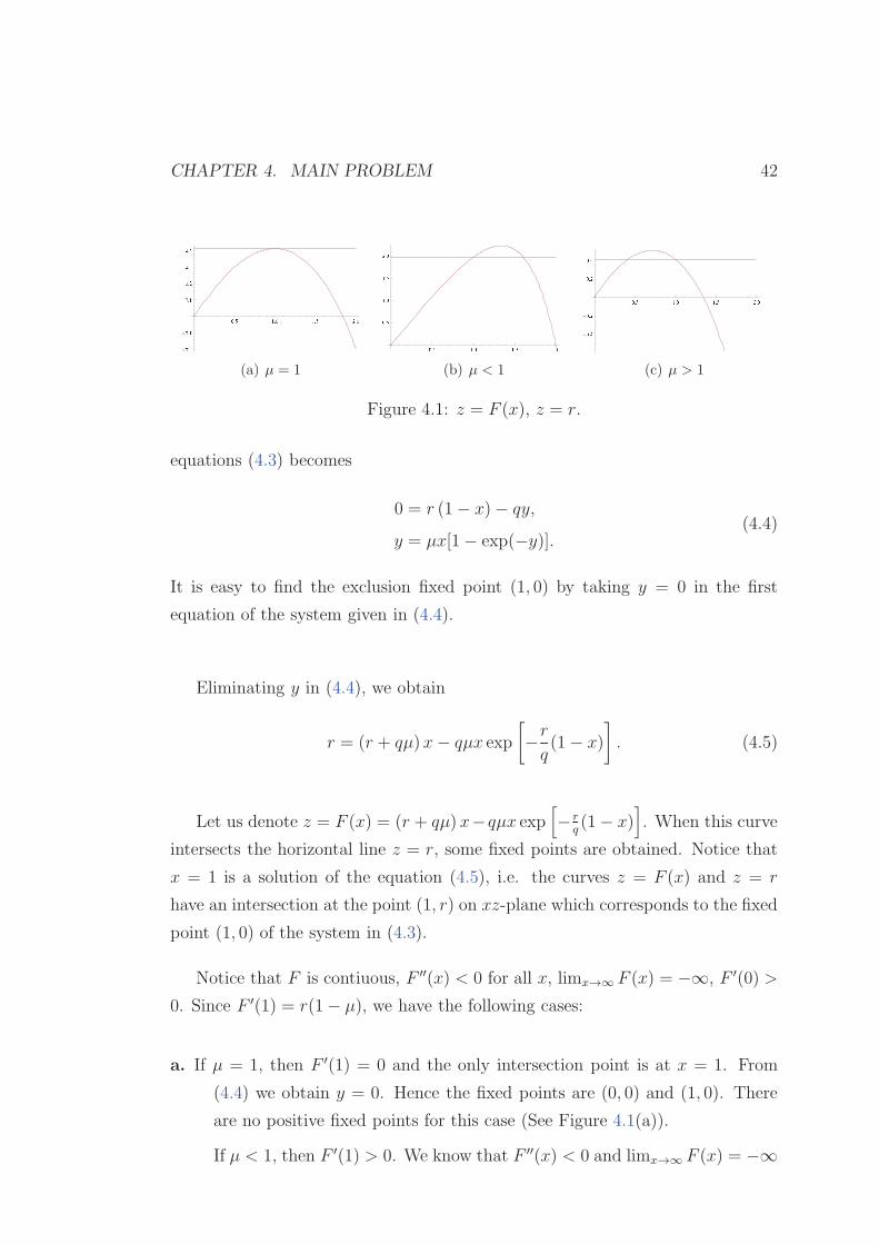
Figure 4.1: z = F (x), z = r.
equations (4.3) becomes
0 = r (1− x)− qy,
y = µx[1− exp(−y)].(4.4)
It is easy to find the exclusion fixed point (1, 0) by taking y = 0 in the first
equation of the system given in (4.4).
Eliminating y in (4.4), we obtain
r = (r + qµ)x− qµx exp
[
−r
q(1− x)
]
. (4.5)
Let us denote z = F (x) = (r + qµ) x−qµx exp[
− rq(1− x)
]
. When this curve
intersects the horizontal line z = r, some fixed points are obtained. Notice that
x = 1 is a solution of the equation (4.5), i.e. the curves z = F (x) and z = r
have an intersection at the point (1, r) on xz-plane which corresponds to the fixed
point (1, 0) of the system in (4.3).
Notice that F is contiuous, F ′′(x) < 0 for all x, limx→∞ F (x) = −∞, F ′(0) >
0. Since F ′(1) = r(1− µ), we have the following cases:
a. If µ = 1, then F ′(1) = 0 and the only intersection point is at x = 1. From
(4.4) we obtain y = 0. Hence the fixed points are (0, 0) and (1, 0). There
are no positive fixed points for this case (See Figure 4.1(a)).
If µ < 1, then F ′(1) > 0. We know that F ′′(x) < 0 and limx→∞ F (x) = −∞
CHAPTER 4. MAIN PROBLEM 43
for all x. This means that there exists another fixed point which is different
from (1, 0). Let us denote the x-component of this fixed point by x = ω,
then ω > 1. We have y = rq(1− ω) < 0 by (4.4) (See Figure 4.1(b)). Since
one component of (ω, rq(1−ω)) is negative, this fixed point is not of interest
in biology and hence it will be omitted.
b. If µ > 1, then F ′(1) < 0. We know that F ′′(x) < 0 for all x and F ′(0) > 0.
Hence there exists another fixed point which is different from (1, 0). Let
us denote the x-component of this fixed point by x = `. Then ` < 1 and
hence y = rq(1 − `) > 0 by (4.4) (See Figure 4.1(c)). Hence (`, r
q(1 − `)) is
the coexistence fixed point.
Lemma 4.2 Let f : R → R be in C2 where f ′(x) > 0, f ′′(x) < 0 for all x ∈ R,
and let g(x) = αx + β where α, β ∈ R and α < 0. Furthermore, assume that
y = f(x) and y = g(x) have an intersection point at (x, y) (Note that, there isn’t
another intersection point.). Take any point (x0, y0) on the curve y = f(x) such
that x0 > x.
Then, the line tangent to the curve y = f(x) at the point (x0, y0) intersects
g(x) at the point (x1, y1) where y < y1 < y0.
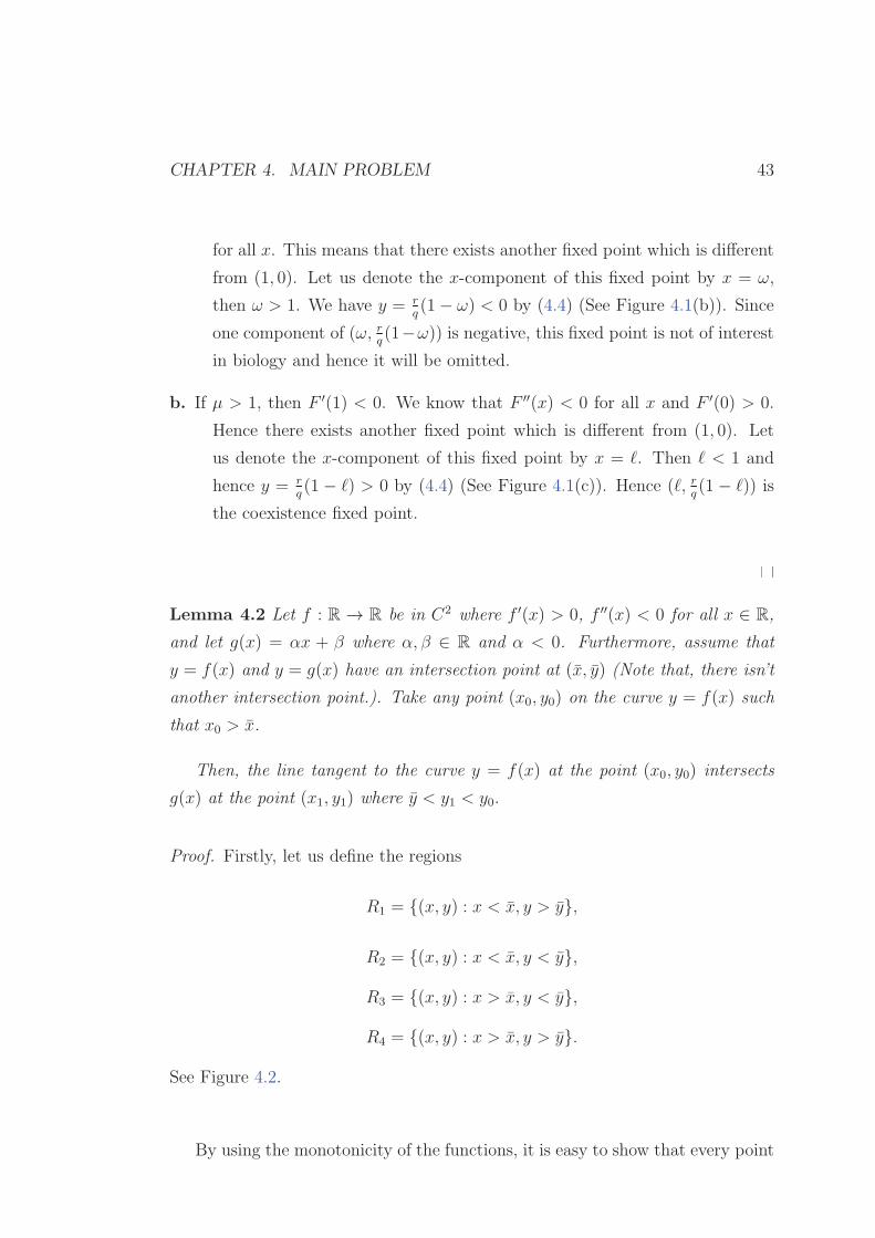
Proof. Firstly, let us define the regions
R1 = {(x, y) : x < x, y > y},
R2 = {(x, y) : x < x, y < y},
R3 = {(x, y) : x > x, y < y},
R4 = {(x, y) : x > x, y > y}.
See Figure 4.2.
By using the monotonicity of the functions, it is easy to show that every point
CHAPTER 4. MAIN PROBLEM 44
on the curve y = f(x) lay in the set R2∪R4∪{(x, y)}. Similarly, the line y = g(x)
lays in the set R1 ∪R3 ∪ {(x, y)}.Take any point (x0, y0) on the curve y = f(x) such that x0 > x. Since f ′′(x) < 0,
H. / 0L
1 21 3 1 4
1 5Figure 4.2: Regions R1, R2, R3, R4.
except the tangent point, every point of the tangent line at (x0, y0) is above the
curve y = f(x). The tangent line and the line y = g(x) intersect at some point
(xg, y1) since the slopes of the lines have different signs. The point (xg, y1) is
above the function y = f(x). The points on the line y = g(x) which are above
the curve y = f(x) must be in the set R1. Hence, the intersection occurs in that
region which guaranties that y < y1. And, since the tangent line is monotonically
increasing, xg < x0 implies y1 < y0. So, we have the desired result, y < y1 < y0
(See Figure 4.3).
Now we construct an iteration in order to approach the intersection point of
the graphs of the two functions in Lemma (4.2).
Let (x0, y0) be a point in the region R4. Now, the tangent line to the curve
y = f(x) and passing through the point (x0, y0) will intersect the line y = g(x)
at a point, let us call it (x1g, y1). Now the horizontal line passing through the
point (x1g, y1) will intersect the curve y = f(x) at a point which will be denoted
CHAPTER 4. MAIN PROBLEM 45
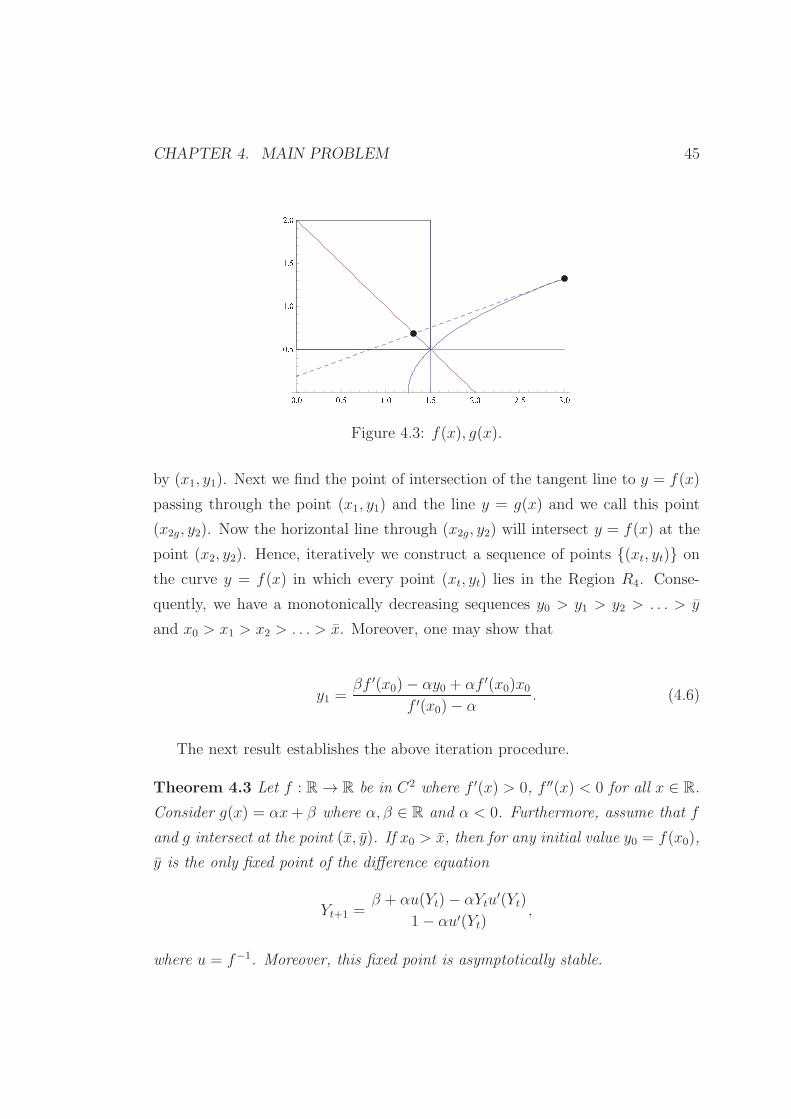
6 7 6 6 7 8 9 7 6 9 7 8 : 7 6 : 7 8 ; 7 66 7 89 7 69 7 8: 7 6
Figure 4.3: f(x), g(x).
by (x1, y1). Next we find the point of intersection of the tangent line to y = f(x)
passing through the point (x1, y1) and the line y = g(x) and we call this point
(x2g, y2). Now the horizontal line through (x2g, y2) will intersect y = f(x) at the
point (x2, y2). Hence, iteratively we construct a sequence of points {(xt, yt)} on
the curve y = f(x) in which every point (xt, yt) lies in the Region R4. Conse-
quently, we have a monotonically decreasing sequences y0 > y1 > y2 > . . . > y
and x0 > x1 > x2 > . . . > x. Moreover, one may show that
y1 =βf ′(x0)− αy0 + αf ′(x0)x0
f ′(x0)− α. (4.6)
The next result establishes the above iteration procedure.
Theorem 4.3 Let f : R→ R be in C2 where f ′(x) > 0, f ′′(x) < 0 for all x ∈ R.
Consider g(x) = αx+ β where α, β ∈ R and α < 0. Furthermore, assume that f
and g intersect at the point (x, y). If x0 > x, then for any initial value y0 = f(x0),
y is the only fixed point of the difference equation
Yt+1 =β + αu(Yt)− αYtu
′(Yt)
1− αu′(Yt),
where u = f−1. Moreover, this fixed point is asymptotically stable.
CHAPTER 4. MAIN PROBLEM 46
Proof. In order to find the fixed points we solve the following equation:
Y =β + αu(Y )− αY u′(Y )
1− αu′(Y ).
Hence, we obtain
Y = αf−1(Y ) + β. (4.7)
It is clear that y is a solution. Since the function f is increasing (f ′(x) > 0),
so is f−1. Hence, by the fact that the function at the left-hand side of equation
(4.7) is increasing and the one on the right-hand side is decreasing, there can be
only one solution. We conclude that Y = y is the only solution.
By Lemma 4.2, Yt is decreasing and bounded below. Hence, its limit is the
fixed point Y = y.
Now, we are ready to focus on the isoclines of system (4.2):
y = −r
qx+
r
q,
y = µx(
1− e−y)
.(4.8)
By Theorem 4.3 we have
g(x) = −r
qx+
r
q,
x = f−1(y) =y
µ (1− e−y).
(4.9)
By Lemma 4.1, if µ > 1 we have a positive fixed point which means that the
isoclines have a point of intersection. We have α = − rq< 0 and β = r
q. Moreover,
f ′(x) > 0 and f ′′(x) < 0. Hence, by Theorem 4.3, the difference equation that
have y as its fixed point is given by
yt+1 =r (µ+ e2ytµ− eyt (y2t + 2µ))
qµ+ e2yt(r + qµ)− eyt(r + ryt + 2qµ)= G(yt). (4.10)
CHAPTER 4. MAIN PROBLEM 47
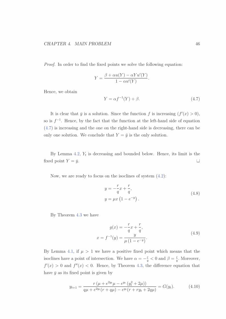
<= =
6 7 : 6 7 > 6 7 ? 6 7 @ 9 7 6 < A6 7 :6 7 >6 7 ?6 7 @9 7 6BH
< AL
Figure 4.4: yt+1 = G(yt).µ = 2.1, r = 2.7, q = 1.2.
The graph of the function yt+1 = G(yt), in equation (4.10), is given in Figure
4.4 for some particular values of parameters.
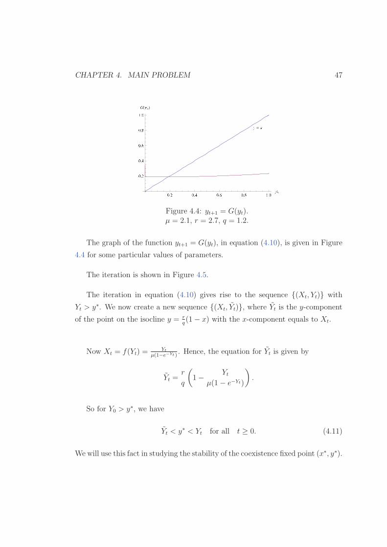
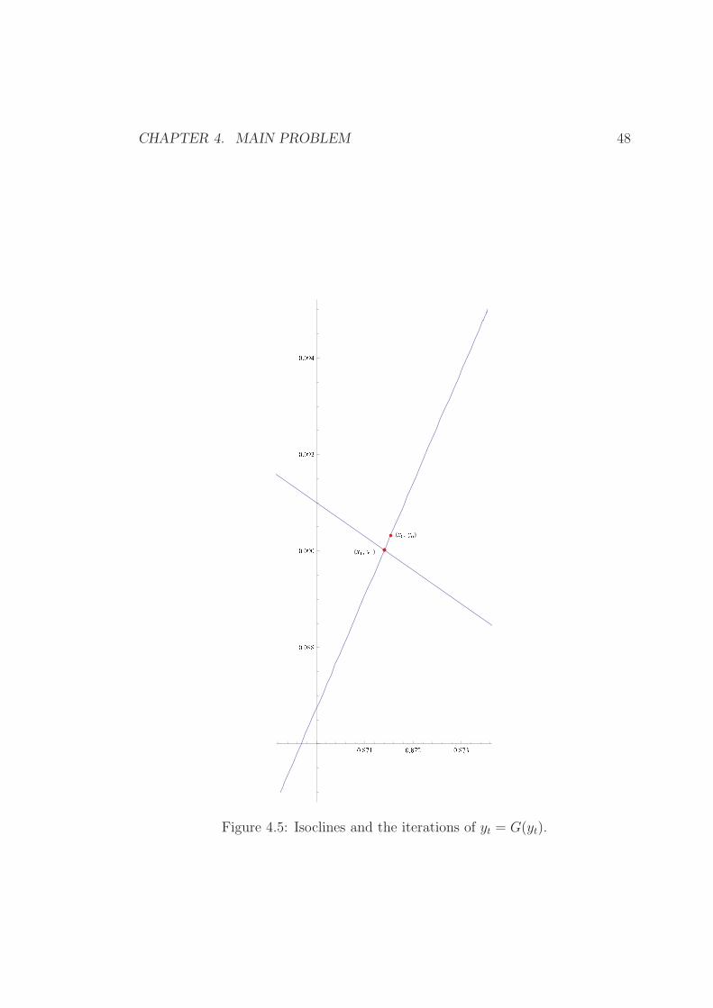
The iteration is shown in Figure 4.5.
The iteration in equation (4.10) gives rise to the sequence {(Xt, Yt)} with
Yt > y∗. We now create a new sequence {(Xt, Yt)}, where Yt is the y-component
of the point on the isocline y = rq(1− x) with the x-component equals to Xt.
Now Xt = f(Yt) =Yt
µ(1−e−Yt ). Hence, the equation for Yt is given by
Yt =r
q
(
1− Yt
µ(1− e−Yt)
)
.
So for Y0 > y∗, we have
Yt < y∗ < Yt for all t ≥ 0. (4.11)
We will use this fact in studying the stability of the coexistence fixed point (x∗, y∗).
CHAPTER 4. MAIN PROBLEM 48
HC D E F D
L
HC G E F G
L
H I J K L H I J K M H I J K NH I H J JH I H O HH I H O MH I H O P
Figure 4.5: Isoclines and the iterations of yt = G(yt).

CHAPTER 4. MAIN PROBLEM 49
4.1.2 Stability of Fixed Points for system (4.2)
4.1.2.1 Stability of extinction and exclusion fixed points
Theorem 4.4 For system (4.2), the following statements hold true:
a. (0, 0) is unstable.
b. (1, 0) is asymptotically stable if 0 < µ < 1 and 0 < r ≤ 2 or 0 < µ ≤ 1 and
0 < r < 2.
Proof. The Jacobian matrix of the map
G(x, y) = (x exp [r (1− x)− qy] , µx[1− exp(−y)])
is
JG(x, y) =
(
er−rx−qy(1− rx) −qer−rx−qyxµ− e−yµ e−yµx
)
.
a. The Jacobian evaluated at the point (0, 0) is
JG(0, 0) =
(
er 0
0 0
)
.
The eigenvalues of JG(0, 0) are 0 and er. Since r > 0, er > 1. Thus (0, 0)
is unstable. We also notice that any point with the form (0, y) is eventually
fixed point, because starting with (0, y), we get G(0, y) = (0, 0).
b. The Jacobian evaluated at (1, 0) is
JG(1, 0) =
(
1− r −q0 µ
)
.
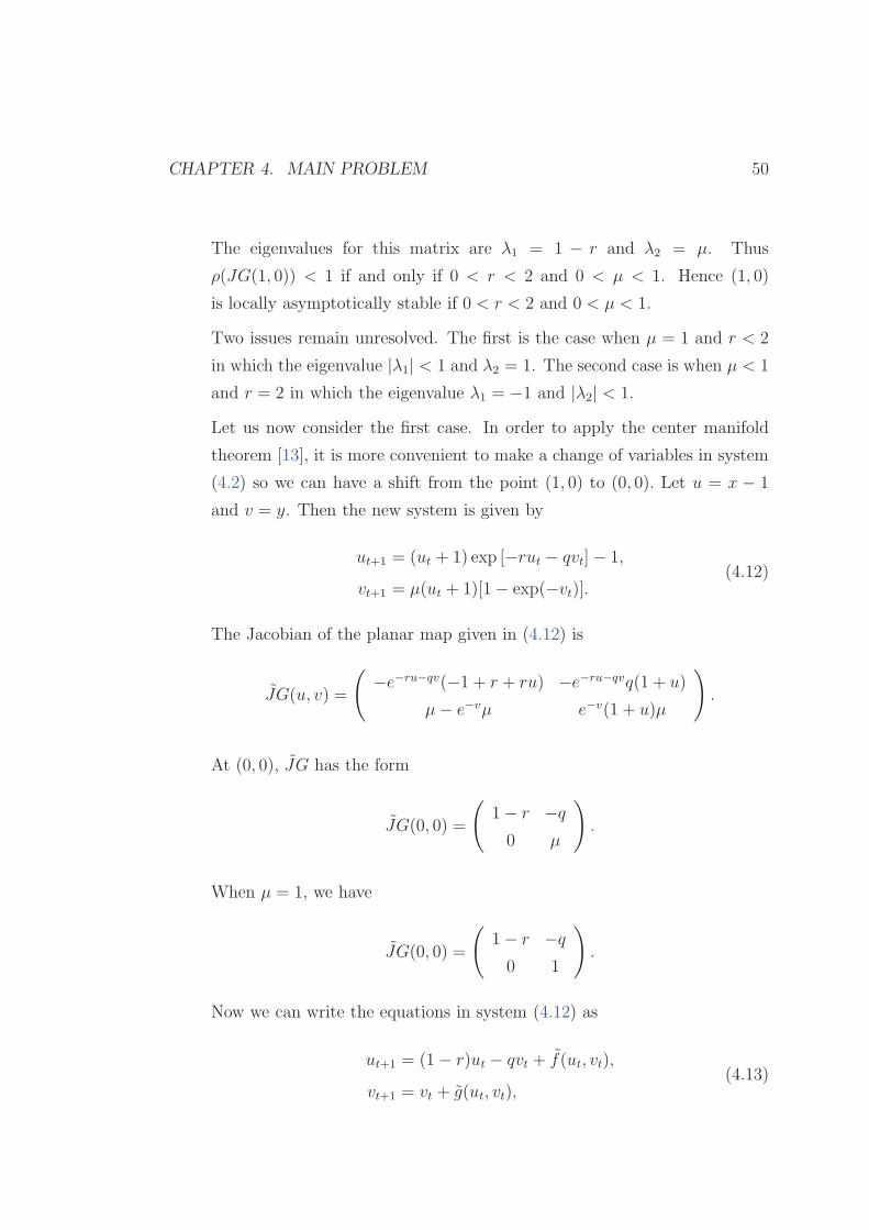
CHAPTER 4. MAIN PROBLEM 50
The eigenvalues for this matrix are λ1 = 1 − r and λ2 = µ. Thus
ρ(JG(1, 0)) < 1 if and only if 0 < r < 2 and 0 < µ < 1. Hence (1, 0)
is locally asymptotically stable if 0 < r < 2 and 0 < µ < 1.
Two issues remain unresolved. The first is the case when µ = 1 and r < 2
in which the eigenvalue |λ1| < 1 and λ2 = 1. The second case is when µ < 1
and r = 2 in which the eigenvalue λ1 = −1 and |λ2| < 1.
Let us now consider the first case. In order to apply the center manifold
theorem [13], it is more convenient to make a change of variables in system
(4.2) so we can have a shift from the point (1, 0) to (0, 0). Let u = x − 1
and v = y. Then the new system is given by
ut+1 = (ut + 1) exp [−rut − qvt]− 1,
vt+1 = µ(ut + 1)[1− exp(−vt)].(4.12)
The Jacobian of the planar map given in (4.12) is
JG(u, v) =
(
−e−ru−qv(−1 + r + ru) −e−ru−qvq(1 + u)
µ− e−vµ e−v(1 + u)µ
)
.
At (0, 0), JG has the form
JG(0, 0) =
(
1− r −q0 µ
)
.
When µ = 1, we have
JG(0, 0) =
(
1− r −q0 1
)
.
Now we can write the equations in system (4.12) as
ut+1 = (1− r)ut − qvt + f(ut, vt),
vt+1 = vt + g(ut, vt),(4.13)
CHAPTER 4. MAIN PROBLEM 51
where
f(ut, vt) = −1 + (−1 + r)ut + e−rut−qvt(1 + ut) + qvt
and
g(ut, vt) = µ(1 + ut)− µe−vt(1 + ut)− vt.
Since invariant manifold is tangent to the corresponding eigenspace by The-
orem 2.9, let us assume that the map h takes the form
h(v) = −q
rv + αv2 + βv3 +O(v4), α, β ∈ R.
Now we are going to compute the constants α and β. The function h must
satisfy the center manifold equation
h(v + g(h(v), v))−[
(1− r)h(v) + qv − f(h(v), v)]
= 0.
The Taylor series expansions, at the point v = 0, are evaluated for the
equation above. Equating the coefficients of the series, we obtain the system
of equationsq2
r2+
q
2r+ αr = 0
and
3q2 + 6r2(α− βr) + qr (1 + 6α(3 + r)) = 0.
Solving the system we get
α = −q(2q + r)
2r3,
β =q (−15qr + (−3 + r)r2 − 6q2(3 + r))
6r5.
Thus on the center manifold u = h(v) we have the following map
P (v) =1
6
(
6− 6qv
r− 3q(2q + r)v2
r3+
q (−15qr + (−3 + r)r2 − 6q2(3 + r)) v3
r5
)
×(
1− e−v)
.
CHAPTER 4. MAIN PROBLEM 52
-6 7 9 6
-6 7 6 8 6 7 6 8 6 7 9 6
-6 7 9 6-6 7 6 86 7 6 86 7 9 68Q / R
<
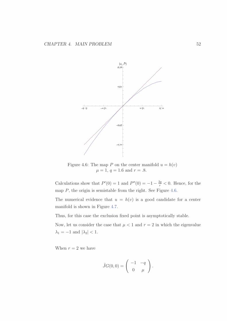
Figure 4.6: The map P on the center manifold u = h(v)µ = 1, q = 1.6 and r = .8.
Calculations show that P ′(0) = 1 and P ′′(0) = −1− 2qr< 0. Hence, for the
map P , the origin is semistable from the right. See Figure 4.6.
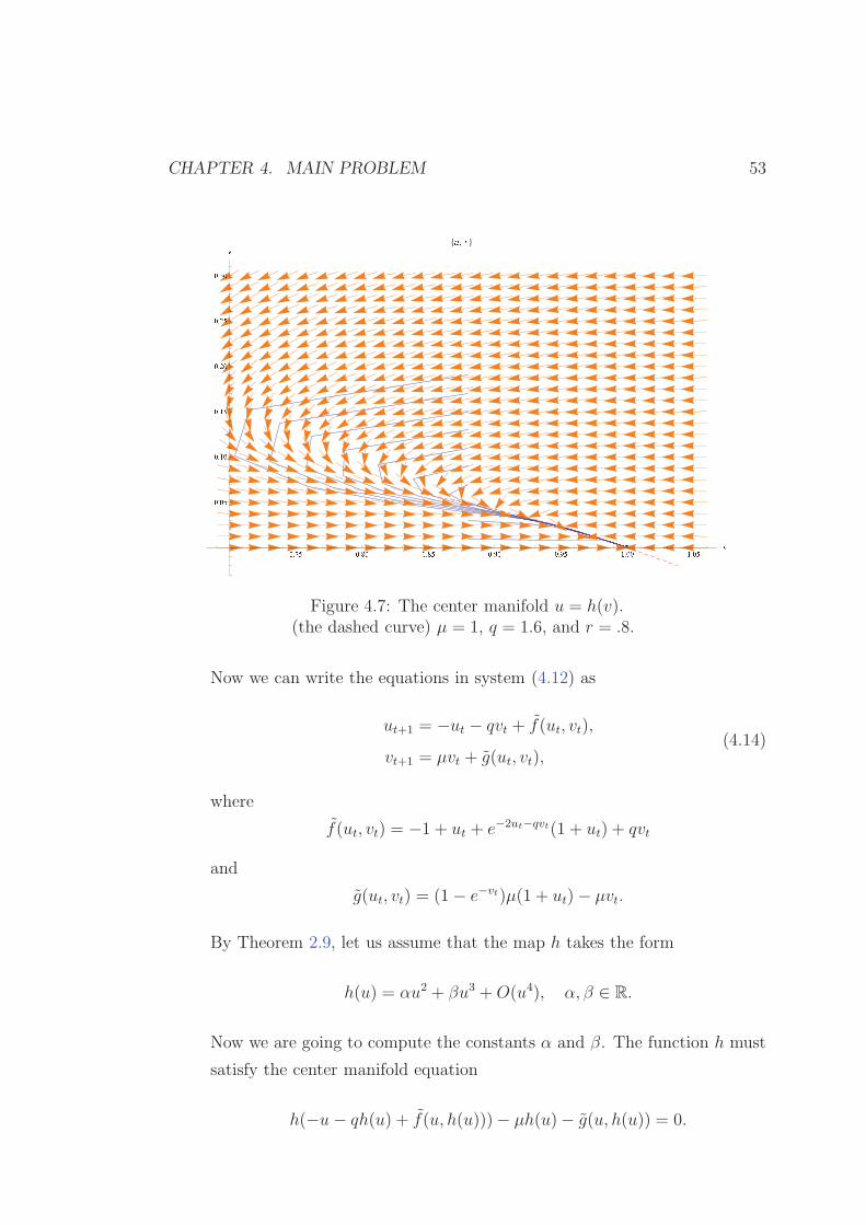
The numerical evidence that u = h(v) is a good candidate for a center
manifold is shown in Figure 4.7.
Thus, for this case the exclusion fixed point is asymptotically stable.
Now, let us consider the case that µ < 1 and r = 2 in which the eigenvalue
λ1 = −1 and |λ2| < 1.
When r = 2 we have
JG(0, 0) =
(
−1 −q0 µ
)
.
CHAPTER 4. MAIN PROBLEM 53
S T U V S T W S S T W V S T X S S T X V Y T S S Y T S V ZS T S VS T Y SS T Y VS T [ SS T [ VS T \ S ] 8_ `<
Figure 4.7: The center manifold u = h(v).(the dashed curve) µ = 1, q = 1.6, and r = .8.
Now we can write the equations in system (4.12) as
ut+1 = −ut − qvt + f(ut, vt),
vt+1 = µvt + g(ut, vt),(4.14)
where
f(ut, vt) = −1 + ut + e−2ut−qvt(1 + ut) + qvt
and
g(ut, vt) = (1− e−vt)µ(1 + ut)− µvt.
By Theorem 2.9, let us assume that the map h takes the form
h(u) = αu2 + βu3 +O(u4), α, β ∈ R.
Now we are going to compute the constants α and β. The function h must
satisfy the center manifold equation
h(−u − qh(u) + f(u, h(u)))− µh(u)− g(u, h(u)) = 0.
CHAPTER 4. MAIN PROBLEM 54
Solving the above functional equation yields:
α− αµ = 0
and
2α2q − αµ− β(1 + µ) = 0.
Hence, α = β = 0. Hence h(u) = 0. Thus on the center manifold v = 0 we
have the following map
Q(u) = −1 + e−2u(1 + u).
Simple calculations show that Q′(0) = −1. The Schwarzian derivative of
the map Q at the origin is −4 < 0. Hence, the exclusion fixed point (1, 0)
is asymptotically stable.
4.1.2.2 The estimation of the stability region of the coexistence fixed
point in the parameter space
In this section, the estimation of the stability region of the coexistence fixed point
in r-µ parameter space is presented.
Lemma 4.5 For the functions f, g, f , g : R2 → R, let
A = {(a, b) : f(a, b) < g(a, b)},
A = {(a, b) : f(a, b) < g(a, b)}.
If f(a, b) < f(a, b) and g(a, b) < g(a, b) for all a, b ∈ R, then A ⊂ A.
Proof. For A = ∅, it is trivial. Now let A 6= ∅. Take (x0, y0) ∈ A. Then f(x0, y0) <
g(x0, y0). Hence, f(x0, y0) < f(x0, y0) < g(x0, y0) < g(x0, y0) from which we
conclude that (x0, y0) ∈ A. Thus, A ⊂ A.
CHAPTER 4. MAIN PROBLEM 55
In Section 4.1.1, we give a symbolic approximation of the coexistence fixed
point. To obtain the stability region for the fixed point, we use equation (4.11),
Lemma 4.5 and the following Trace-Determinant Formula:
|Tr(J∗)| − 1 < Det(J∗) < 1,
where J∗ is the Jacobian matrix evaluated at the coexistence fixed point.
It is equivalent to
Det(J∗) < 1 ∧ Det(J∗) > Tr(J∗)− 1 ∧ Det(J∗) > −Tr(J∗)− 1.
Firstly, we convert the Jacobian of the system at the coexistence fixed point
(x∗, y∗) to the following form in which, x∗ is eliminated:
J∗ =
(
1− r + qy∗ −q + q2y∗
r
ry∗
r−qy∗µ− y∗ − µqy∗
r
)
.
The determinant and the trace of J∗ are:
Det (J∗) =1
r
[
r2(y∗ − µ)− qy∗(1 + qy∗)µ+ r(
−qy∗2 + µ+ y∗(−1 + q + 2qµ))]
,
T r (J∗) = 1− r + (−1 + q)y∗ + µ− qy∗µ
r.
Case 1. Det(J∗) < 1
The region on r-µ parameter space for the condition Det(J∗) < 1 is given by
A = {(r, µ) : µr − µr2 − r + (2µrq + r2 + qr)y∗ < (qr + q2µ)y∗2 + (r + qµ)y∗}.
Let
At = {(r, µ) : µr−µr2−r+(2µrq+r2+qr)Yt < (qr+q2µ)Y 2t +(r+qµ)Yt}. (4.15)
CHAPTER 4. MAIN PROBLEM 56
By Lemma 4.5 and the bounds in equation (4.11), we have At ⊂ A for all t ≥ 0.
Similarly, we obtain A0 ⊂ A1 ⊂ A2 ⊂ · · · ⊂ At ⊂ · · · ⊂ A. Hence, for every point
(r, µ) in the region At, the condition Det(J∗) < 1 is satisfied for any t.
Case 2. Tr(J∗) < 1 +Det(J∗)
By using the similar idea as Case 1, we convert this inequality to the form where
both sides are monotonic functions with respect to y∗ and use the bounds in
equation (4.11) to obtain the region
Bt = {(r, µ) : r2 − µr2 + (2µqr + r2)Yt > (µq2 + qr)Yt2}. (4.16)
Case 3. −1 −Det(J∗) < Tr(J∗)
For this case, similarly we obtain the region
Ct = {(r, µ) : −2r − 2µr + r2 + µr2 + (2µq + 2r)Yt + (mq2 + qr)Yt2 <
(
2mqr + r2 + 2qr)
Yt}.(4.17)
In order to obtain the stability region in the (r, µ) plane, let us take q = 1.6.
By numeric computations, we obtain the regions A5, B5, and C5 which are
subsets of the regions satisfying Det(J∗) < 1, Det(J∗) > Tr(J∗) − 1 and
Det(J∗) > −Tr(J∗) − 1, respectively. Since the intersection of the sets A5, B5,
and C5 is a subset of the stability region, finally, we obtain the approximated sta-
bility region of the coexistence fixed point. Furthermore, on the borderline of the
stability region, we have Neimark-Sacker bifurcation when Det(J∗) = 1; saddle-
node bifurcation when Det(J∗) = Tr(J∗) − 1 and period-doubling bifurcation
when Det(J∗) = −Tr(J∗) − 1. In Figure 4.8, the approximated stability region
and the types of bifurcation appearing on the borderline of the region is presented.
The approximated stability region for some particular values of parameter q
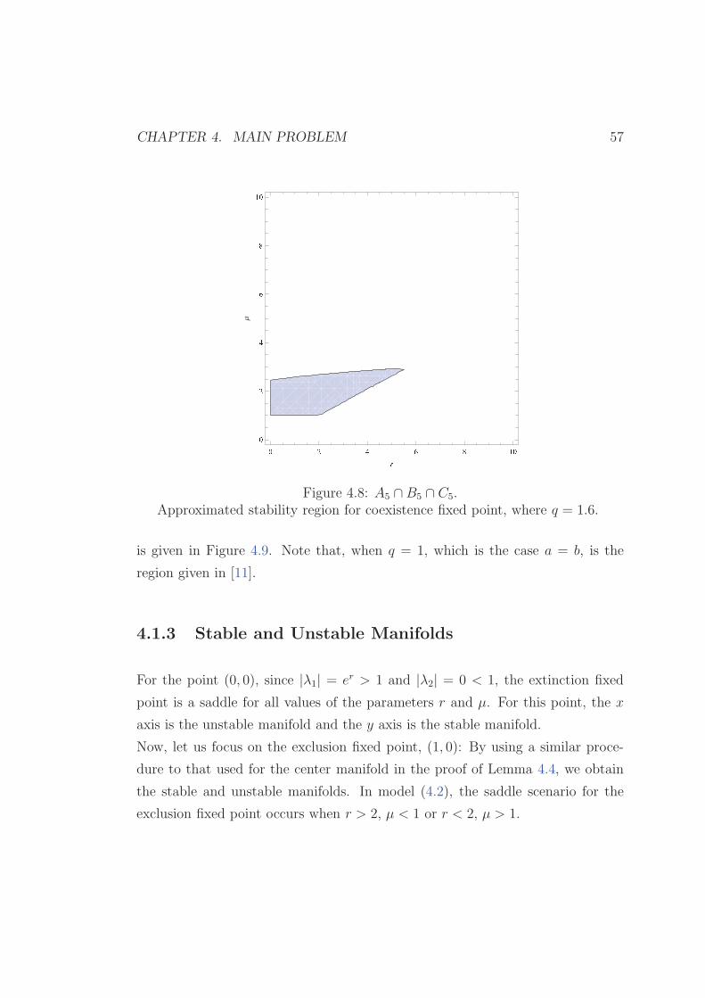
CHAPTER 4. MAIN PROBLEM 57
6 : > ? @ 9 66:>?@9 6
a
Μ
Figure 4.8: A5 ∩B5 ∩ C5.Approximated stability region for coexistence fixed point, where q = 1.6.
is given in Figure 4.9. Note that, when q = 1, which is the case a = b, is the
region given in [11].
4.1.3 Stable and Unstable Manifolds
For the point (0, 0), since |λ1| = er > 1 and |λ2| = 0 < 1, the extinction fixed
point is a saddle for all values of the parameters r and µ. For this point, the x
axis is the unstable manifold and the y axis is the stable manifold.
Now, let us focus on the exclusion fixed point, (1, 0): By using a similar proce-
dure to that used for the center manifold in the proof of Lemma 4.4, we obtain
the stable and unstable manifolds. In model (4.2), the saddle scenario for the
exclusion fixed point occurs when r > 2, µ < 1 or r < 2, µ > 1.
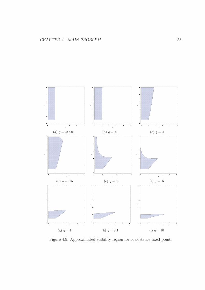
CHAPTER 4. MAIN PROBLEM 58
b c d e f g bbcdefg b
hΜ
(a) q = .00001
b c d e f g bbcdefg b
hΜ
(b) q = .01
b c d e f g bbcdefg b
hΜ
(c) q = .1
b c d e f g bbcdefg b
hΜ
(d) q = .15
b c d e f g bbcdefg b
hΜ
(e) q = .5
b c d e f g bbcdefg b
hΜ
(f) q = .6
b c d e f g bbcdefg b
hΜ
(g) q = 1
b c d e f g bbcdefg b
hΜ
(h) q = 2.4
b c d e f g bbcdefg b
hΜ
(i) q = 10
Figure 4.9: Approximated stability region for coexistence fixed point.
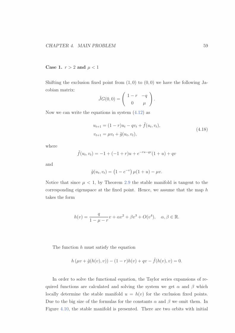
CHAPTER 4. MAIN PROBLEM 59
Case 1. r > 2 and µ < 1
Shifting the exclusion fixed point from (1, 0) to (0, 0) we have the following Ja-
cobian matrix:
JG(0, 0) =
(
1− r −q0 µ
)
.
Now we can write the equations in system (4.12) as
ut+1 = (1− r)ut − qvt + f(ut, vt),
vt+1 = µvt + g(ut, vt),(4.18)
where
f(ut, vt) = −1 + (−1 + r)u+ e−ru−qv(1 + u) + qv
and
g(ut, vt) =(
1− e−v)
µ(1 + u)− µv.
Notice that since µ < 1, by Theorem 2.9 the stable manifold is tangent to the
corresponding eigenspace at the fixed point. Hence, we assume that the map h
takes the form
h(v) =q
1− µ− rv + αv2 + βv3 +O(v4), α, β ∈ R.
The function h must satisfy the equation
h (µv + g(h(v), v))− (1− r)h(v) + qv − f(h(v), v) = 0.
In order to solve the functional equation, the Taylor series expansions of re-
quired functions are calculated and solving the system we get α and β which
locally determine the stable manifold u = h(v) for the exclusion fixed points.
Due to the big size of the formulas for the constants α and β we omit them. In
Figure 4.10, the stable manifold is presented. There are two orbits with initial
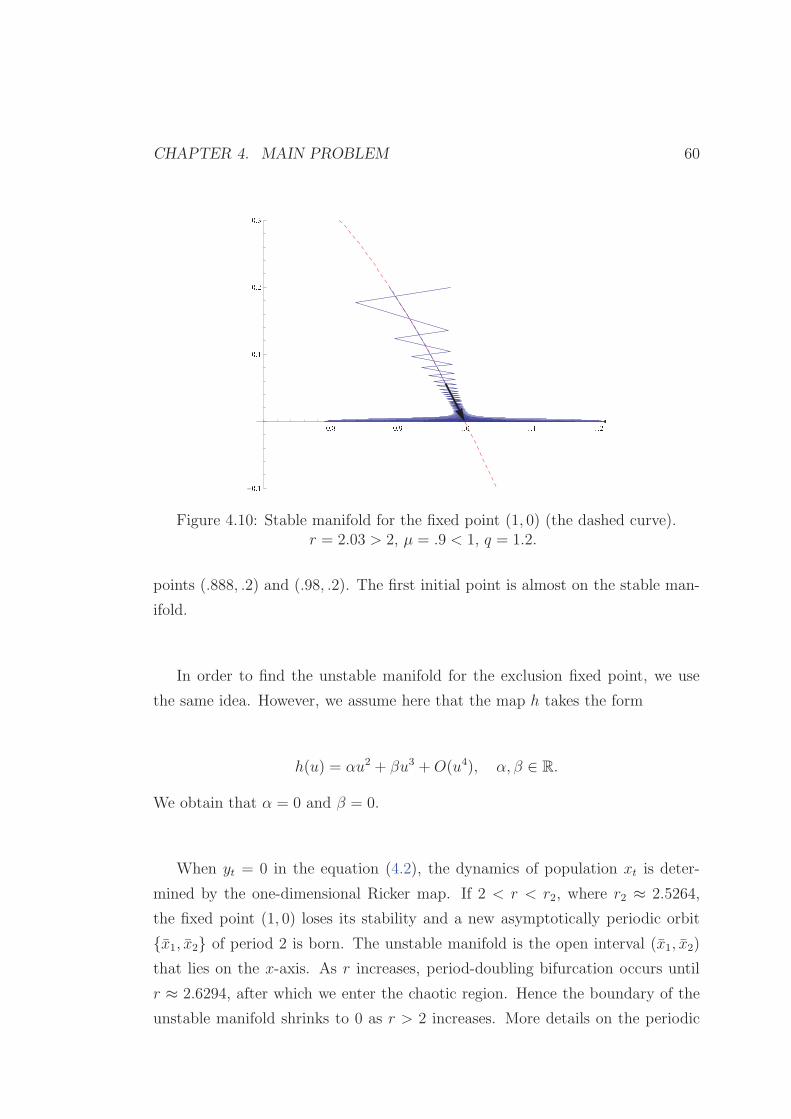
CHAPTER 4. MAIN PROBLEM 60
H I J H I O L I H L I L L I M-
H I LH I LH I MH I N
Figure 4.10: Stable manifold for the fixed point (1, 0) (the dashed curve).r = 2.03 > 2, µ = .9 < 1, q = 1.2.
points (.888, .2) and (.98, .2). The first initial point is almost on the stable man-
ifold.
In order to find the unstable manifold for the exclusion fixed point, we use
the same idea. However, we assume here that the map h takes the form
h(u) = αu2 + βu3 +O(u4), α, β ∈ R.
We obtain that α = 0 and β = 0.
When yt = 0 in the equation (4.2), the dynamics of population xt is deter-
mined by the one-dimensional Ricker map. If 2 < r < r2, where r2 ≈ 2.5264,
the fixed point (1, 0) loses its stability and a new asymptotically periodic orbit
{x1, x2} of period 2 is born. The unstable manifold is the open interval (x1, x2)
that lies on the x-axis. As r increases, period-doubling bifurcation occurs until
r ≈ 2.6294, after which we enter the chaotic region. Hence the boundary of the
unstable manifold shrinks to 0 as r > 2 increases. More details on the periodic
CHAPTER 4. MAIN PROBLEM 61
points of the Ricker map and the basin of attractions of its periodic orbits may
be found in [15].
Case 2. r < 2 and µ > 1
In order to find the unstable manifold for this case; since invariant manifold is
tangent to the corresponding eigenspace by Theorem 2.9, let us assume that the
map h takes the form
h(v) =q
1− µ− rv + αv2 + βv3 +O(v4), α, β ∈ R.
Since µ > 1, the unstable manifold is tangent to the corresponding eigenvector
at the fixed point.
Since the method we use for this case is the same as in the previous case, we
omit the details.
In order to find the stable manifold for the exclusion fixed point, we assume that
the map h takes the form
h(u) = αu2 + βu3 +O(u4), α, β ∈ R.
See Figure 4.11.
4.1.4 Bifurcation Scenarios
In this section, a bifurcation diagram for the positive fixed point is presented.
In Figure 4.13, Tr-Det Diagram for a general system is shown. We give the
corresponding regions for system (4.2) in Figure 4.14: Bi is the corresponding
region for Ai.
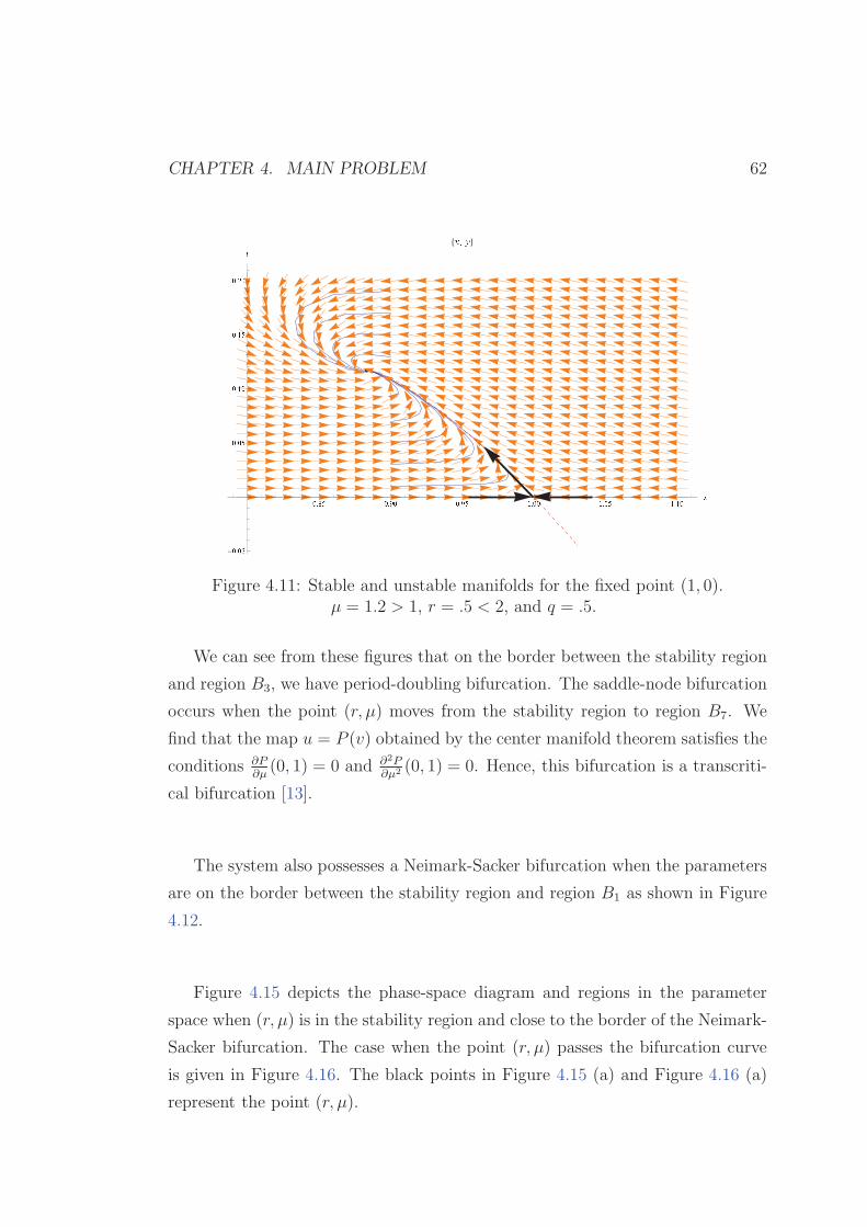
CHAPTER 4. MAIN PROBLEM 62
S T W V S T X S S T X V Y T S S Y T S V Y T Y S i-
S T S VS T S VS T Y SS T Y VS T [ S j 8
k _ l<
Figure 4.11: Stable and unstable manifolds for the fixed point (1, 0).µ = 1.2 > 1, r = .5 < 2, and q = .5.
We can see from these figures that on the border between the stability region
and region B3, we have period-doubling bifurcation. The saddle-node bifurcation
occurs when the point (r, µ) moves from the stability region to region B7. We
find that the map u = P (v) obtained by the center manifold theorem satisfies the
conditions ∂P∂µ(0, 1) = 0 and ∂2P
∂µ2 (0, 1) = 0. Hence, this bifurcation is a transcriti-
cal bifurcation [13].
The system also possesses a Neimark-Sacker bifurcation when the parameters
are on the border between the stability region and region B1 as shown in Figure
4.12.
Figure 4.15 depicts the phase-space diagram and regions in the parameter
space when (r, µ) is in the stability region and close to the border of the Neimark-
Sacker bifurcation. The case when the point (r, µ) passes the bifurcation curve
is given in Figure 4.16. The black points in Figure 4.15 (a) and Figure 4.16 (a)
represent the point (r, µ).
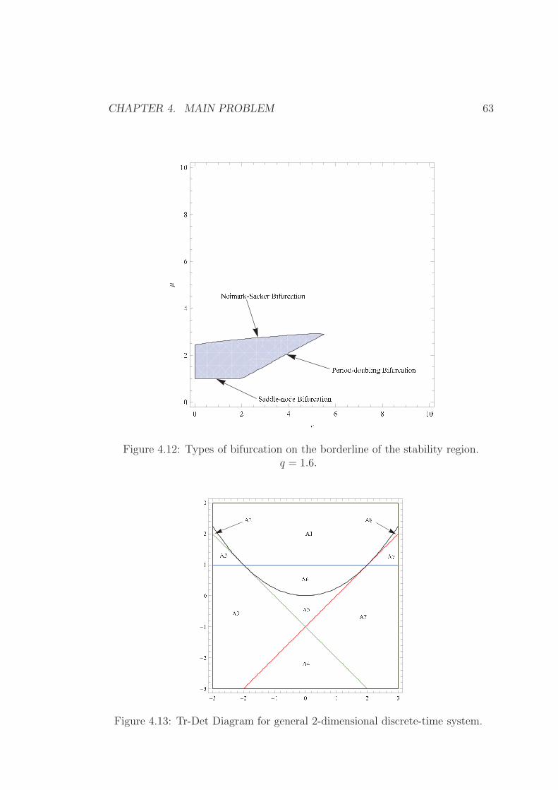
CHAPTER 4. MAIN PROBLEM 63
m n o p q r s t u q v s n r w o x y r v q z o { |} n r o { ~ t ~ { y � � o | � w o x y r v q z o { |u q ~ ~ � n t | { ~ n w o x y r v q z o { |� � � � � � ����
��� �
�
Μ
Figure 4.12: Types of bifurcation on the borderline of the stability region.q = 1.6.
� 9� :� ; � ; � >� 8� ? � �� �� @
-;
-:
-9 6 9 : ;-
;- :- 969:;
Figure 4.13: Tr-Det Diagram for general 2-dimensional discrete-time system.
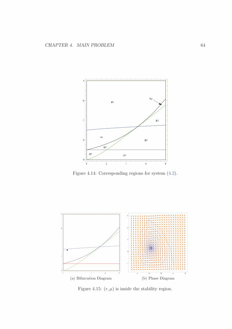
CHAPTER 4. MAIN PROBLEM 64
� 9� ? � 8� � � > � ; � ;� :
6 : > ? @6:>?@
Figure 4.14: Corresponding regions for system (4.2).
b c d e fbcdef
(a) Bifurcation Diagram
� �� � �� � �� � �� � ��� ��� ��� ��� ��� ��
(b) Phase Diagram
Figure 4.15: (r, µ) is inside the stability region.
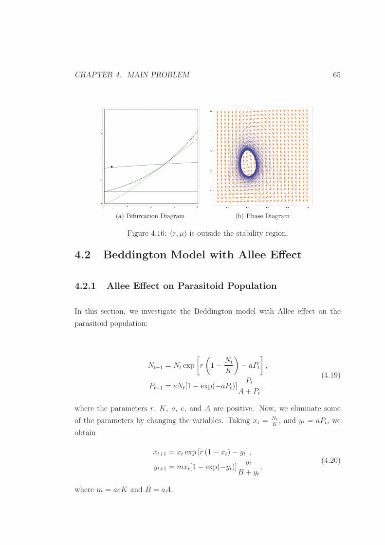
CHAPTER 4. MAIN PROBLEM 65
� � � � ������
(a) Bifurcation Diagram
� �� � �� � �� � �� � ��� ��� ��� ��� ��� ��
(b) Phase Diagram
Figure 4.16: (r, µ) is outside the stability region.
4.2 Beddington Model with Allee Effect
4.2.1 Allee Effect on Parasitoid Population
In this section, we investigate the Beddington model with Allee effect on the
parasitoid population:
Nt+1 = Nt exp
[
r
(
1− Nt
K
)
− aPt
]
,
Pt+1 = eNt[1− exp(−aPt)]Pt
A+ Pt
,
(4.19)
where the parameters r, K, a, e, and A are positive. Now, we eliminate some
of the parameters by changing the variables. Taking xt =Nt
K, and yt = aPt, we
obtain
xt+1 = xt exp [r (1− xt)− yt] ,
yt+1 = mxt[1− exp(−yt)]yt
B + yt,
(4.20)
where m = aeK and B = aA.
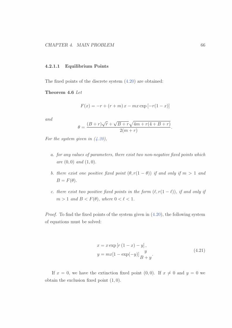
CHAPTER 4. MAIN PROBLEM 66
4.2.1.1 Equilibrium Points
The fixed points of the discrete system (4.20) are obtained:
Theorem 4.6 Let
F (x) = −r + (r +m)x−mx exp [−r(1− x)]
and
θ =(B + r)
√r +
√B + r
√
4m+ r(4 +B + r)
2(m+ r).
For the system given in (4.20),
a. for any values of parameters, there exist two non-negative fixed points which
are (0, 0) and (1, 0).
b. there exist one positive fixed point (θ, r(1 − θ)) if and only if m > 1 and
B = F (θ).
c. there exist two positive fixed points in the form (`, r(1 − `)), if and only if
m > 1 and B < F (θ), where 0 < ` < 1.
Proof. To find the fixed points of the system given in (4.20), the following system
of equations must be solved:
x = x exp [r (1− x)− y] ,
y = mx[1− exp(−y)] y
B + y.
(4.21)
If x = 0, we have the extinction fixed point (0, 0). If x 6= 0 and y = 0 we
obtain the exclusion fixed point (1, 0).
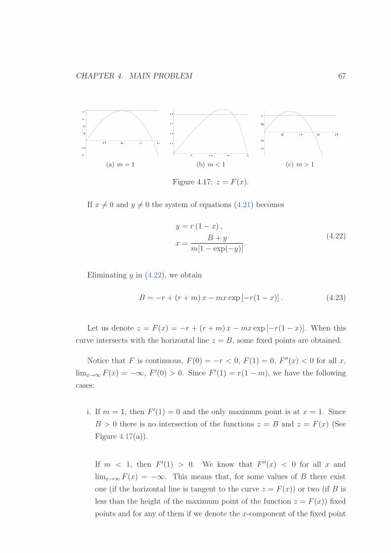
CHAPTER 4. MAIN PROBLEM 67
� � � � � � � � � � � �-
� � �-� � �� � �� � �� � �� � �
(a) m = 1
� � � � � � � � � � � �� � �� � �� � �� � �(b) m < 1
� � � � � � � � � � � �-
� � �-� � �� � �� � �
(c) m > 1
Figure 4.17: z = F (x).
If x 6= 0 and y 6= 0 the system of equations (4.21) becomes
y = r (1− x) ,
x =B + y
m[1− exp(−y)] .(4.22)
Eliminating y in (4.22), we obtain
B = −r + (r +m) x−mx exp [−r(1 − x)] . (4.23)
Let us denote z = F (x) = −r + (r +m) x −mx exp [−r(1− x)]. When this
curve intersects with the horizontal line z = B, some fixed points are obtained.
Notice that F is continuous, F (0) = −r < 0, F (1) = 0, F ′′(x) < 0 for all x,
limx→∞ F (x) = −∞, F ′(0) > 0. Since F ′(1) = r(1 −m), we have the following
cases:
i. If m = 1, then F ′(1) = 0 and the only maximum point is at x = 1. Since
B > 0 there is no intersection of the functions z = B and z = F (x) (See
Figure 4.17(a)).
If m < 1, then F ′(1) > 0. We know that F ′′(x) < 0 for all x and
limx→∞ F (x) = −∞. This means that, for some values of B there exist
one (if the horizontal line is tangent to the curve z = F (x)) or two (if B is
less than the height of the maximum point of the function z = F (x)) fixed
points and for any of them if we denote the x-component of the fixed point
CHAPTER 4. MAIN PROBLEM 68
by x = ω, then ω > 1. We have y = r(1 − ω) < 0 by the first equation of
system (4.22) (See Figure 4.17(b)). Since one component of (ω, r(1−ω)) is
negative, this fixed point is not of interest in biology and hence it will be
omitted.
ii. If m > 1, then F ′(1) < 0. We know that F ′′(x) < 0 for all x and
F (0) = −r < 0. Hence, for some values of B there exist one (if the hori-
zontal line is tangent to the curve z = F (x)) or two (if B is less than the
height of the maximum point of the function z = F (x)) fixed points. Let
us denote the x-component of this fixed point by x = `. Then ` < 1 and
hence y = r(1 − `) > 0 by (4.22) (See Figure 4.17(c)). Hence, (`, r(1 − `))
is a candidate to be a coexistence fixed point.
Now, we have to determine that in which condition the horizontal line z = B
intersects the function z = F (x) for m > 1. That is the condition when
the number B is less than the height of the maximum value of the curve
z = F (x). Let us denote the maximum point by (x, y). In order to find
that point, we have
F ′(x) = r −m(
−1 + er(−1+x)(1 + rx))
= 0.
We focus on the case where the horizontal line z = B is tangent to the
curve z = F (x), that is F (x) = B:
−r + (r +m) x−mx exp [−r(1− x)] = B.
Eliminating the term er(1−x) in the two equations above, we obtain
− r + (m+ r)x− (m+ r)x
1 + rx= B. (4.24)
The positive solution of equation (4.24) for x is as follows:
x =(B + r)
√r +
√B + r
√
4m+ r(4 +B + r)
2(m+ r). (4.25)
CHAPTER 4. MAIN PROBLEM 69
Hence, the condition for existence of the positive fixed point in part (b) and
(c) is obtained: There exist one intersection point (x, r(1− x)) if and only
if m > 1 and B = F (x). And there exist two intersection points if and only
if m > 1 and B < F (x).
4.2.1.2 Stability of Fixed Points for System (4.20)
Theorem 4.7 For system (4.20), the following statements hold true:
a. (0, 0) is unstable.
b. if 0 < r ≤ 2, then (1, 0) is asymptotically stable .
Proof. The Jacobian matrix of the map
G(x, y) =
(
xer(1−x)−y, mx(1− e−y)y
B + y
)
is
JG(x, y) =
er−rx−y(1− rx) −er−rx−yx(1−e−y)my
B+y
e−ymx(y2+B(−1+ey+y))(B+y)2
.
a. The Jacobian evaluated at the point (0, 0) is
JG(0, 0) =
(
er 0
0 0
)
.
The eigenvalues of JG(0, 0) are 0 and er. Since r > 0, er > 1. Thus (0, 0)
is unstable. We also notice that any point with the form (0, y) is eventually
fixed point, because starting with (0, y), we get (0, 0) after one iteration.
CHAPTER 4. MAIN PROBLEM 70
b. The Jacobian evaluated at (1, 0) is
JG(1, 0) =
(
1− r −10 0
)
.
The eigenvalues for this matrix are λ1 = 1 − r and λ2 = 0. Thus, the
fixed point (1, 0) is locally asymptotically stable if ρ(JG(1, 0)) < 1, that
is 0 < r < 2. If r > 2, the fixed point (1, 0) is unstable. If r = 2, then
the eigenvalue are λ1 = −1 and λ2 = 0. Now, we have to apply the center
manifold theorem [13]: by changing variables, let u = x − 1 and v = y in
system (4.20), we have a shift from the point (1, 0) to (0, 0). Then the new
system is given by
ut+1 = (ut + 1) exp [−rut − vt]− 1,
vt+1 = m(ut + 1)[1− exp(−vt)]vt
B + vt.
(4.26)
The Jacobian of the planar map given in (4.26) is
JG(u, v) =
−e−ru−v(−1 + r + ru) −e−ru−v(1 + u)(1−e−v)mv
B+v
e−vm(1+u)(v2+B(−1+ev+v))(B+v)2
. (4.27)
At (0, 0), JG has the form
JG(0, 0) =
(
1− r −10 0
)
.
When r = 2 we have
JG(0, 0) =
(
−1 −10 0
)
.
Now we can write the equations in system (4.26) as
ut+1 = −ut − vt + f(ut, vt),
vt+1 = g(ut, vt),(4.28)
CHAPTER 4. MAIN PROBLEM 71
where
f(ut, vt) = −1 + ut + e−2ut−vt(1 + ut) + vt
and
g(ut, vt) =(1− e−vt)m(1 + ut)vt
B + vt.
By Theorem 2.9, let us assume that the map v = h(u) takes the form
h(u) = αu2 + βu3 +O(u4), α, β ∈ R.
Now, we are going to compute the constants α and β. The function v = h(u)
must satisfy the center manifold equation
h[
−u− h(u) + f(u, h(u))]
− g(u, h(u)) = 0.
The Taylor series expansion at the point u = 0 is evaluated for the equation
above. Equating the coefficients of the series, we obtain α = β = 0.
Thus on the center manifold v = 0 we have the following map
P (u) = −1 + e−2u(1 + u).
Calculations show that P ′(0) = −1 and Schwarzian derivative of the map
Q at the origin is −43< 0. Hence, the exclusion fixed point (1, 0) is locally
asymptotically stable (See Figure 4.18).
4.2.1.3 Stable and Unstable Manifolds
For the point (0, 0), since |λ1| = er > 1 and |λ2| = 0 < 1, the extinction fixed
point is saddle for any values of parameters r and m. For this point, x axis is
unstable and y axis is stable manifold.
Now, let us focus on the exclusion fixed point, (1, 0): By using the similar proce-
dure that is used for the center manifold in the proof of Theorem 4.7, we obtain
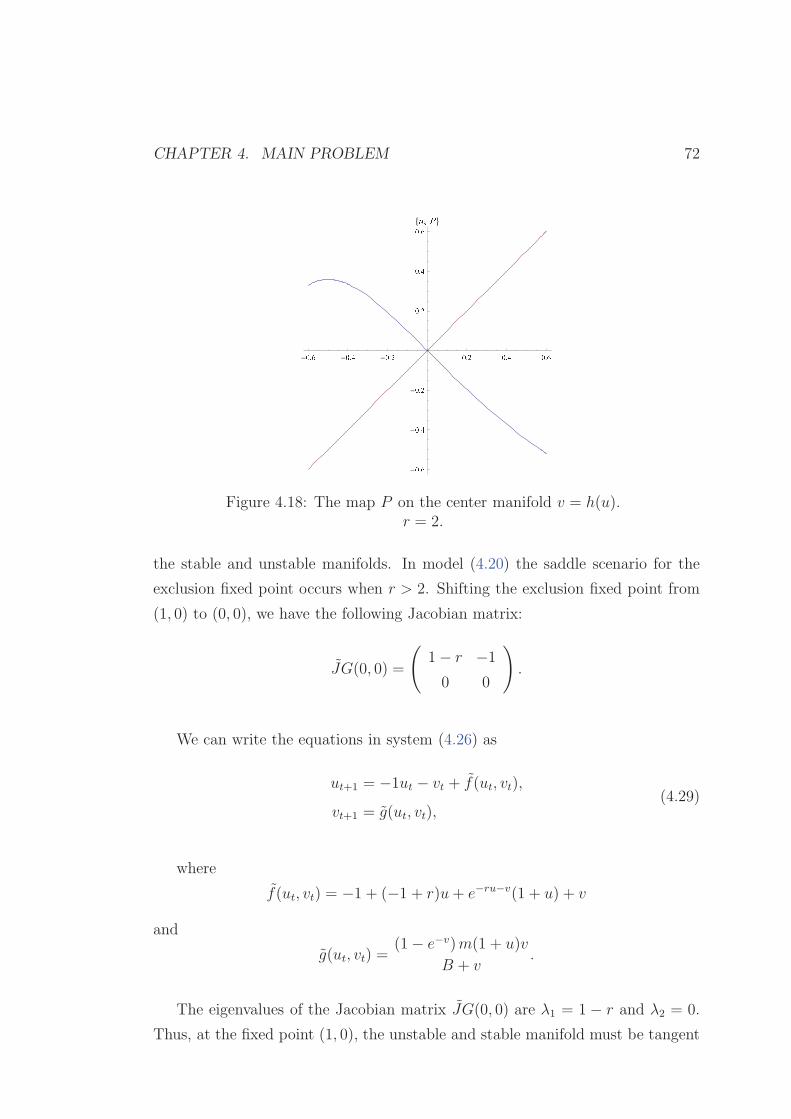
CHAPTER 4. MAIN PROBLEM 72
-� � �
-� � �
-� � � � � � � � � �
-� � �-� � �-� � � � � � �� � �8¡ ¢ £
<
Figure 4.18: The map P on the center manifold v = h(u).r = 2.
the stable and unstable manifolds. In model (4.20) the saddle scenario for the
exclusion fixed point occurs when r > 2. Shifting the exclusion fixed point from
(1, 0) to (0, 0), we have the following Jacobian matrix:
JG(0, 0) =
(
1− r −10 0
)
.
We can write the equations in system (4.26) as
ut+1 = −1ut − vt + f(ut, vt),
vt+1 = g(ut, vt),(4.29)
where
f(ut, vt) = −1 + (−1 + r)u+ e−ru−v(1 + u) + v
and
g(ut, vt) =(1− e−v)m(1 + u)v
B + v.
The eigenvalues of the Jacobian matrix JG(0, 0) are λ1 = 1 − r and λ2 = 0.
Thus, at the fixed point (1, 0), the unstable and stable manifold must be tangent
CHAPTER 4. MAIN PROBLEM 73
to the eigenvectors
(
1
0
)
and
(
1
1− r
)
, respectively.
In order to find the unstable manifold for the exclusion fixed point, we assume
that the map v = h(u) takes the form
h(u) = αu2 + βu3 +O(u4), α, β ∈ R.
The map h must satisfy the following center manifold equation
h(
(1− r)u− h(u) + f(u, h(u)))
− g(u, h(u)) = 0.
The Taylor expansion at the point (0, 0) yields
α(−1 + r)2u2 − (−1 + r)(
−2α2 + β(−1 + r)2 + α(−2 + r)r)
u3 +O[u]4 = 0.
Thus, we obtain α = β = 0. Hence, the unstable manifold is h(u) = 0 and the
map on the unstable manifold is
Q(u) = −1 + e−ru(1 + u).
Notice that |Q′(0)| = |1− r| > 1 when r > 2.
In order to find the stable manifold for the exclusion fixed point, we assume
that map h takes the form
h(v) =1
1− rv + αv2 + βv3 +O(v4), α, β ∈ R.
Hence, the center manifold equation is
h (g(h(v), v))− (1− r)h(v) + v − ˜f(h(v), v) = 0.
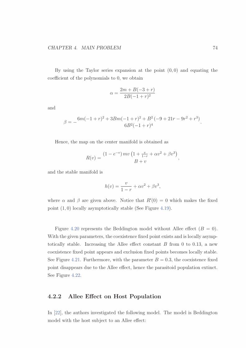
CHAPTER 4. MAIN PROBLEM 74
By using the Taylor series expansion at the point (0, 0) and equating the
coefficient of the polynomials to 0, we obtain
α =2m+B(−3 + r)
2B(−1 + r)2
and
β = −6m(−1 + r)2 + 3Bm(−1 + r)2 +B2 (−9 + 21r − 9r2 + r3)
6B2(−1 + r)4.
Hence, the map on the center manifold is obtained as
R(v) =(1− e−v)mv
(
1 + v1−r
+ αv2 + βv3)
B + v,
and the stable manifold is
h(v) =v
1− r+ αv2 + βv3,
where α and β are given above. Notice that R′(0) = 0 which makes the fixed
point (1, 0) locally asymptotically stable (See Figure 4.19).
Figure 4.20 represents the Beddington model without Allee effect (B = 0).
With the given parameters, the coexistence fixed point exists and is locally asymp-
totically stable. Increasing the Allee effect constant B from 0 to 0.13, a new
coexistence fixed point appears and exclusion fixed points becomes locally stable.
See Figure 4.21. Furthermore, with the parameter B = 0.3, the coexistence fixed
point disappears due to the Allee effect, hence the parasitoid population extinct.
See Figure 4.22.
4.2.2 Allee Effect on Host Population
In [22], the authors investigated the following model. The model is Beddington
model with the host subject to an Allee effect:
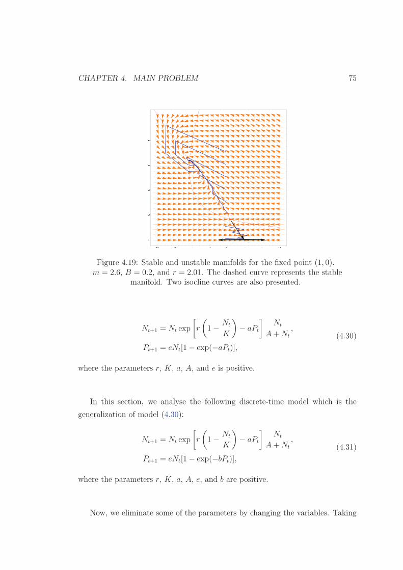
CHAPTER 4. MAIN PROBLEM 75
¤ ¥ ¦ ¤ ¥ § ¤ ¥ ¨ ¤ ¥ © ¤ ¥ ª « ¥ ¤ « ¥ « « ¥ ¬¤ ¥ ¤¤ ¥ ¬¤ ¥ ¤ ¥ §¤ ¥ ©« ¥ ¤
Figure 4.19: Stable and unstable manifolds for the fixed point (1, 0).m = 2.6, B = 0.2, and r = 2.01. The dashed curve represents the stable
manifold. Two isocline curves are also presented.
Nt+1 = Nt exp
[
r
(
1− Nt
K
)
− aPt
]
Nt
A+Nt
,
Pt+1 = eNt[1− exp(−aPt)],
(4.30)
where the parameters r, K, a, A, and e is positive.
In this section, we analyse the following discrete-time model which is the
generalization of model (4.30):
Nt+1 = Nt exp
[
r
(
1− Nt
K
)
− aPt
]
Nt
A+Nt
,
Pt+1 = eNt[1− exp(−bPt)],
(4.31)
where the parameters r, K, a, A, e, and b are positive.
Now, we eliminate some of the parameters by changing the variables. Taking
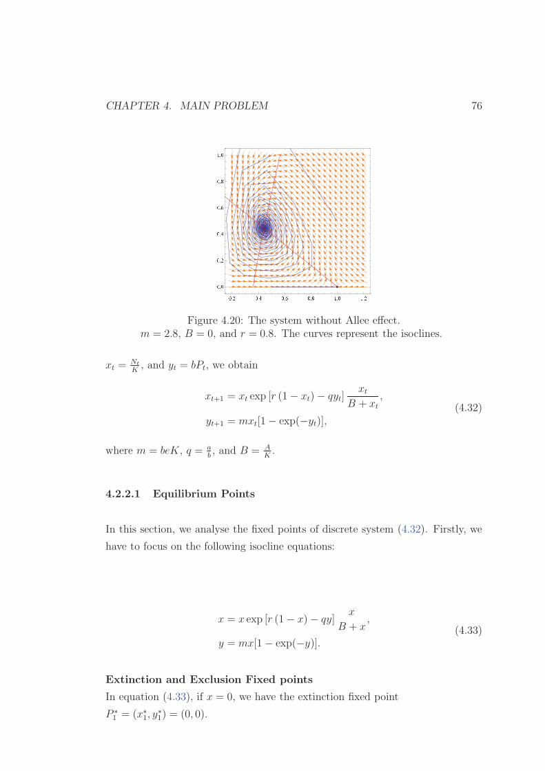
CHAPTER 4. MAIN PROBLEM 76
� � � � � � � � � � ® ¯ � � ¯ � � � �� � � � �� � �� � ®¯ � �
Figure 4.20: The system without Allee effect.m = 2.8, B = 0, and r = 0.8. The curves represent the isoclines.
xt =Nt
K, and yt = bPt, we obtain
xt+1 = xt exp [r (1− xt)− qyt]xt
B + xt
,
yt+1 = mxt[1− exp(−yt)],(4.32)
where m = beK, q = ab, and B = A
K.
4.2.2.1 Equilibrium Points
In this section, we analyse the fixed points of discrete system (4.32). Firstly, we
have to focus on the following isocline equations:
x = x exp [r (1− x)− qy]x
B + x,
y = mx[1 − exp(−y)].(4.33)
Extinction and Exclusion Fixed points
In equation (4.33), if x = 0, we have the extinction fixed point
P ∗
1 = (x∗
1, y∗
1) = (0, 0).
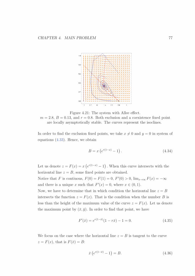
CHAPTER 4. MAIN PROBLEM 77
° ± ° ° ± ² ° ± ³ ° ± ´ ° ± µ ¶ ± ° ¶ ± ²° ± °° ± ²° ± ³° ± ´° ± µ¶ ± °
Figure 4.21: The system with Allee effect.m = 2.8, B = 0.13, and r = 0.8. Both exclusion and a coexistence fixed point
are locally asymptotically stable. The curves represent the isoclines.
In order to find the exclusion fixed points, we take x 6= 0 and y = 0 in system of
equations (4.33). Hence, we obtain
B = x(
er(1−x) − 1)
. (4.34)
Let us denote z = F (x) = x(
er(1−x) − 1)
. When this curve intersects with the
horizontal line z = B, some fixed points are obtained.
Notice that F is contiuous, F (0) = F (1) = 0, F ′(0) > 0, limx→∞ F (x) = −∞and there is a unique x such that F ′(x) = 0, where x ∈ (0, 1).
Now, we have to determine that in which condition the horizontal line z = B
intersects the function z = F (x). That is the condition when the number B is
less than the height of the maximum value of the curve z = F (x). Let us denote
the maximum point by (x, y). In order to find that point, we have
F ′(x) = er(1−x)(1− rx)− 1 = 0. (4.35)
We focus on the case where the horizontal line z = B is tangent to the curve
z = F (x), that is F (x) = B:
x(
er(1−x) − 1)
= B. (4.36)
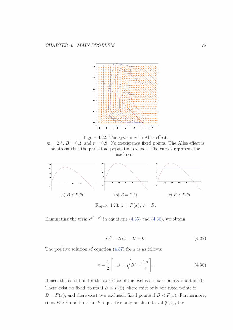
CHAPTER 4. MAIN PROBLEM 78
� � � � � � � � � � � � � ® ¯ � � ¯ � � � �� � � � �� � �� � ®¯ � �
Figure 4.22: The system with Allee effect.m = 2.8, B = 0.3, and r = 0.8. No coexistence fixed points. The Allee effect isso strong that the parasitoid population extinct. The curves represent the
isoclines.
� � � � � � � � � � � � � � � � � �-
� � �� � �� � �� � �� � �(a) B > F (θ)
� � � � � � � � � � � � � � � � � �-
� � �� � �� � �� � �� � �(b) B = F (θ)
� � � � � � � � � � � � � � � � � �-
� � �� � �� � �� � �� � �(c) B < F (θ)
Figure 4.23: z = F (x), z = B.
Eliminating the term er(1−x) in equations (4.35) and (4.36), we obtain
rx2 +Brx− B = 0. (4.37)
The positive solution of equation (4.37) for x is as follows:
x =1
2
[
−B +
√
B2 +4B
r
]
. (4.38)
Hence, the condition for the existence of the exclusion fixed points is obtained:
There exist no fixed points if B > F (x); there exist only one fixed points if
B = F (x); and there exist two exclusion fixed points if B < F (x). Furthermore,
since B > 0 and function F is positive only on the interval (0, 1), the
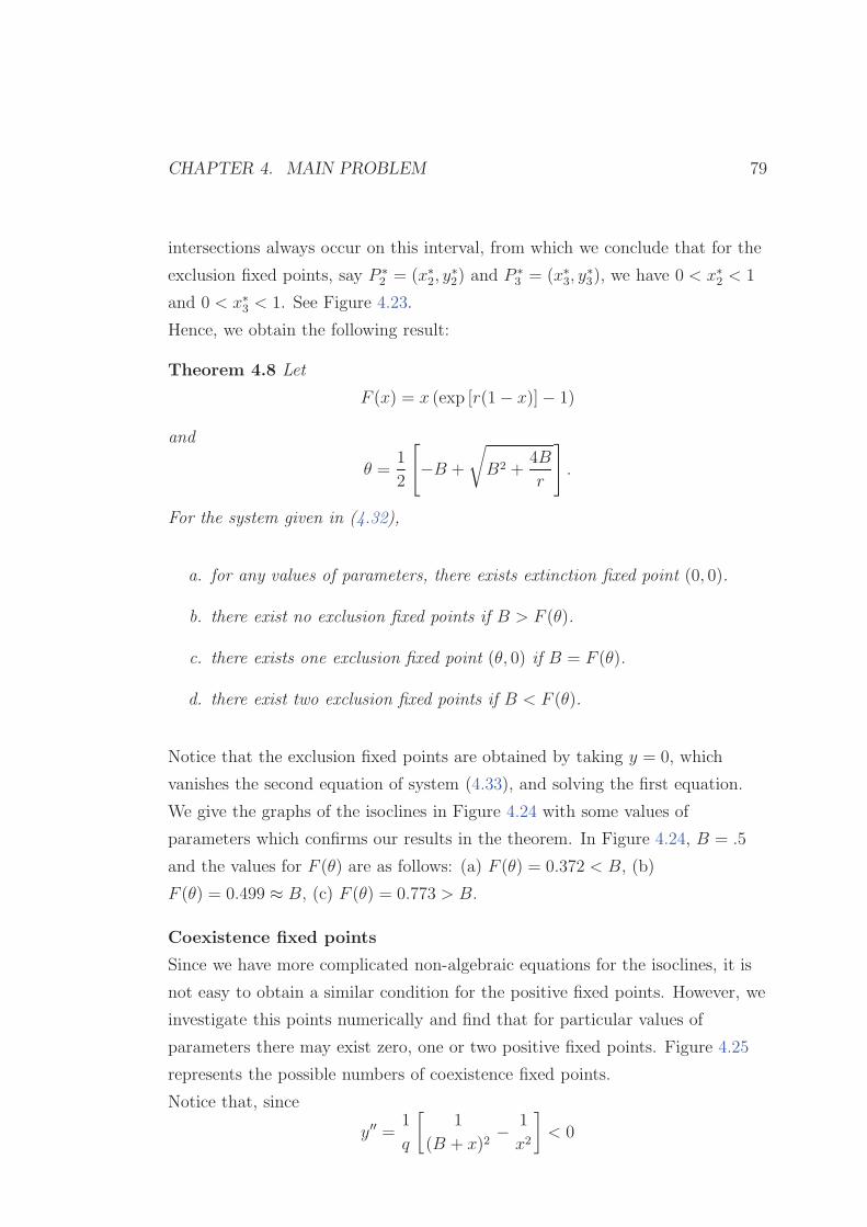
CHAPTER 4. MAIN PROBLEM 79
intersections always occur on this interval, from which we conclude that for the
exclusion fixed points, say P ∗
2 = (x∗
2, y∗
2) and P ∗
3 = (x∗
3, y∗
3), we have 0 < x∗
2 < 1
and 0 < x∗
3 < 1. See Figure 4.23.
Hence, we obtain the following result:
Theorem 4.8 Let
F (x) = x (exp [r(1− x)]− 1)
and
θ =1
2
[
−B +
√
B2 +4B
r
]
.
For the system given in (4.32),
a. for any values of parameters, there exists extinction fixed point (0, 0).
b. there exist no exclusion fixed points if B > F (θ).
c. there exists one exclusion fixed point (θ, 0) if B = F (θ).
d. there exist two exclusion fixed points if B < F (θ).
Notice that the exclusion fixed points are obtained by taking y = 0, which
vanishes the second equation of system (4.33), and solving the first equation.
We give the graphs of the isoclines in Figure 4.24 with some values of
parameters which confirms our results in the theorem. In Figure 4.24, B = .5
and the values for F (θ) are as follows: (a) F (θ) = 0.372 < B, (b)
F (θ) = 0.499 ≈ B, (c) F (θ) = 0.773 > B.
Coexistence fixed points
Since we have more complicated non-algebraic equations for the isoclines, it is
not easy to obtain a similar condition for the positive fixed points. However, we
investigate this points numerically and find that for particular values of
parameters there may exist zero, one or two positive fixed points. Figure 4.25
represents the possible numbers of coexistence fixed points.
Notice that, since
y′′ =1
q
[
1
(B + x)2− 1
x2
]
< 0
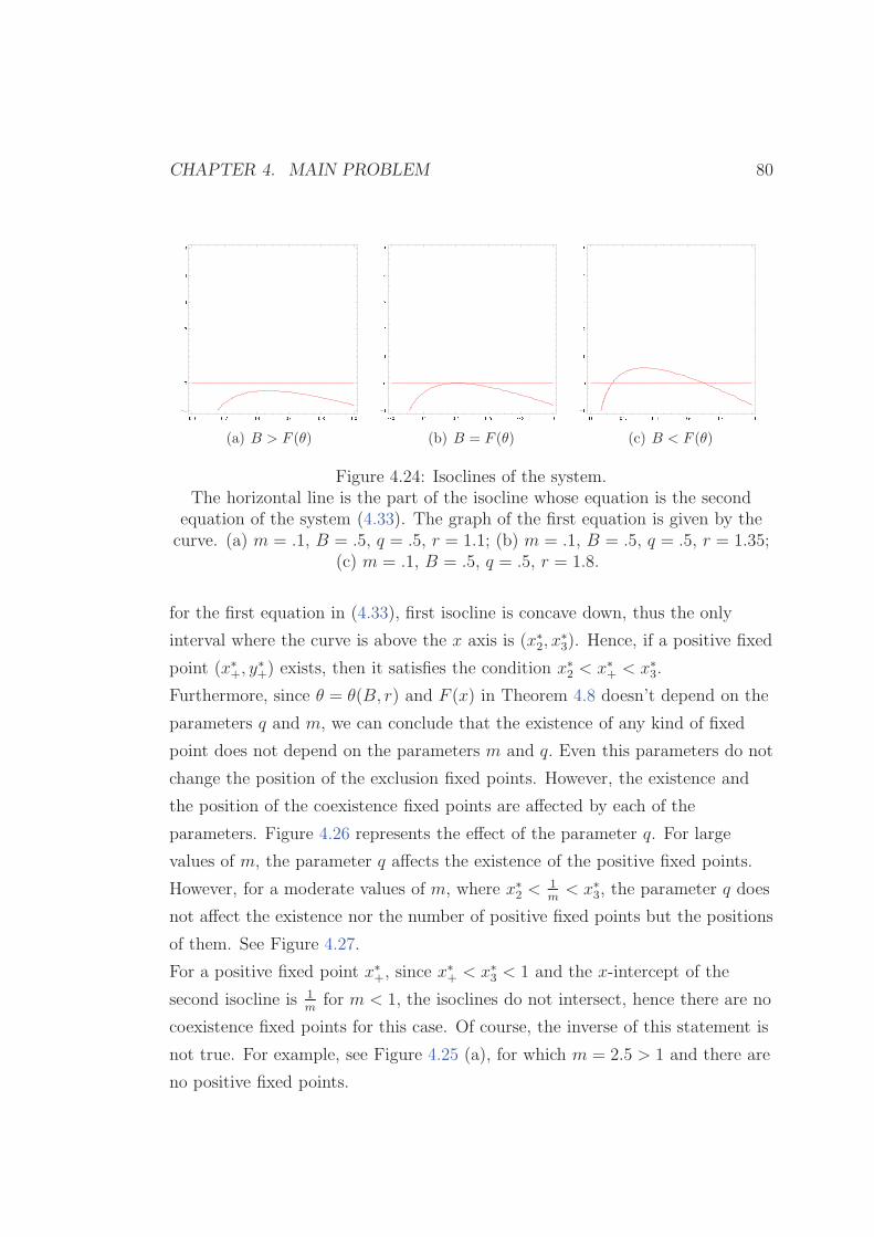
CHAPTER 4. MAIN PROBLEM 80
� � � � � � � � � � � � � � � � � �-�������
(a) B > F (θ)
� � � � � � � � � � � � � � � � � �-�������
(b) B = F (θ)
� � � � � � � � � � � � � � � � � �-�������
(c) B < F (θ)
Figure 4.24: Isoclines of the system.The horizontal line is the part of the isocline whose equation is the second
equation of the system (4.33). The graph of the first equation is given by thecurve. (a) m = .1, B = .5, q = .5, r = 1.1; (b) m = .1, B = .5, q = .5, r = 1.35;
(c) m = .1, B = .5, q = .5, r = 1.8.
for the first equation in (4.33), first isocline is concave down, thus the only
interval where the curve is above the x axis is (x∗
2, x∗
3). Hence, if a positive fixed
point (x∗
+, y∗
+) exists, then it satisfies the condition x∗
2 < x∗
+ < x∗
3.
Furthermore, since θ = θ(B, r) and F (x) in Theorem 4.8 doesn’t depend on the
parameters q and m, we can conclude that the existence of any kind of fixed
point does not depend on the parameters m and q. Even this parameters do not
change the position of the exclusion fixed points. However, the existence and
the position of the coexistence fixed points are affected by each of the
parameters. Figure 4.26 represents the effect of the parameter q. For large
values of m, the parameter q affects the existence of the positive fixed points.
However, for a moderate values of m, where x∗
2 <1m
< x∗
3, the parameter q does
not affect the existence nor the number of positive fixed points but the positions
of them. See Figure 4.27.
For a positive fixed point x∗
+, since x∗
+ < x∗
3 < 1 and the x-intercept of the
second isocline is 1m
for m < 1, the isoclines do not intersect, hence there are no
coexistence fixed points for this case. Of course, the inverse of this statement is
not true. For example, see Figure 4.25 (a), for which m = 2.5 > 1 and there are
no positive fixed points.
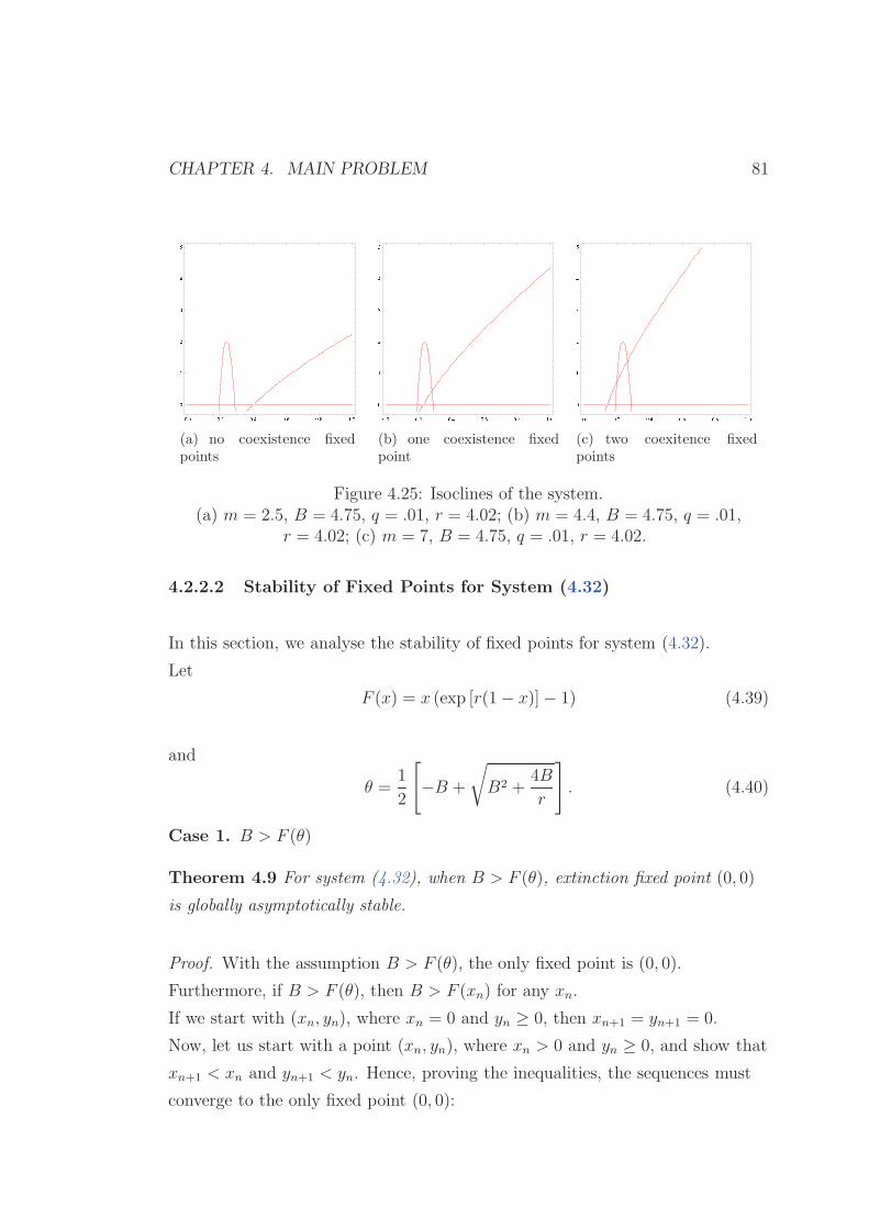
CHAPTER 4. MAIN PROBLEM 81
� � � � � � � � � � � � � � � � � �������(a) no coexistence fixedpoints
� � � � � � � � � � � � � � � � � �������(b) one coexistence fixedpoint
� � � � � � � � � � � � � � � � � �������(c) two coexitence fixedpoints
Figure 4.25: Isoclines of the system.(a) m = 2.5, B = 4.75, q = .01, r = 4.02; (b) m = 4.4, B = 4.75, q = .01,
r = 4.02; (c) m = 7, B = 4.75, q = .01, r = 4.02.
4.2.2.2 Stability of Fixed Points for System (4.32)
In this section, we analyse the stability of fixed points for system (4.32).
Let
F (x) = x (exp [r(1− x)]− 1) (4.39)
and
θ =1
2
[
−B +
√
B2 +4B
r
]
. (4.40)
Case 1. B > F (θ)
Theorem 4.9 For system (4.32), when B > F (θ), extinction fixed point (0, 0)
is globally asymptotically stable.
Proof. With the assumption B > F (θ), the only fixed point is (0, 0).
Furthermore, if B > F (θ), then B > F (xn) for any xn.
If we start with (xn, yn), where xn = 0 and yn ≥ 0, then xn+1 = yn+1 = 0.
Now, let us start with a point (xn, yn), where xn > 0 and yn ≥ 0, and show that
xn+1 < xn and yn+1 < yn. Hence, proving the inequalities, the sequences must
converge to the only fixed point (0, 0):
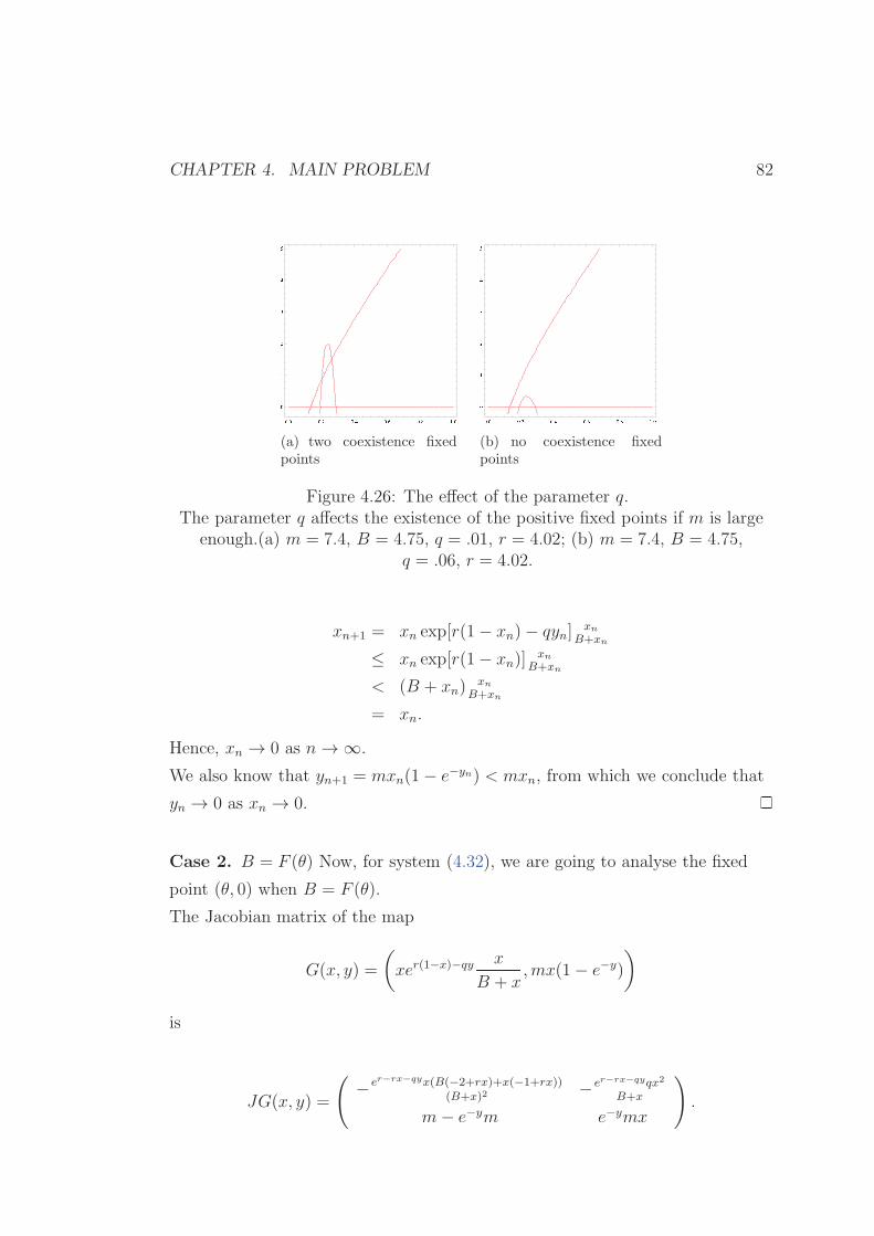
CHAPTER 4. MAIN PROBLEM 82
� � � � � � � � � � � � � � � � � �������(a) two coexistence fixedpoints
� � � � � � � � � � � � � � � � � �������(b) no coexistence fixedpoints
Figure 4.26: The effect of the parameter q.The parameter q affects the existence of the positive fixed points if m is large
enough.(a) m = 7.4, B = 4.75, q = .01, r = 4.02; (b) m = 7.4, B = 4.75,q = .06, r = 4.02.
xn+1 = xn exp[r(1− xn)− qyn]xn
B+xn
≤ xn exp[r(1− xn)]xn
B+xn
< (B + xn)xn
B+xn
= xn.
Hence, xn → 0 as n→∞.
We also know that yn+1 = mxn(1− e−yn) < mxn, from which we conclude that
yn → 0 as xn → 0.
Case 2. B = F (θ) Now, for system (4.32), we are going to analyse the fixed
point (θ, 0) when B = F (θ).
The Jacobian matrix of the map
G(x, y) =
(
xer(1−x)−qy x
B + x,mx(1− e−y)
)
is
JG(x, y) =
(
−er−rx−qyx(B(−2+rx)+x(−1+rx))(B+x)2
−er−rx−qyqx2
B+x
m− e−ym e−ymx
)
.
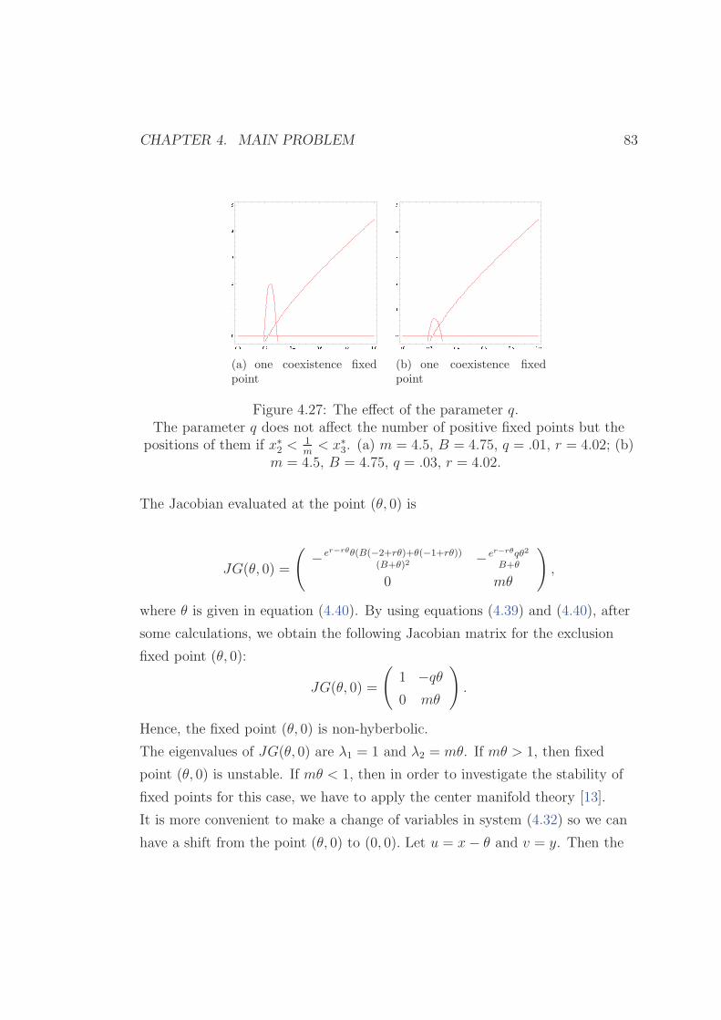
CHAPTER 4. MAIN PROBLEM 83
� � � � � � � � � � � � � � � � � �������(a) one coexistence fixedpoint
� � � � � � � � � � � � � � � � � �������(b) one coexistence fixedpoint
Figure 4.27: The effect of the parameter q.The parameter q does not affect the number of positive fixed points but the
positions of them if x∗
2 <1m
< x∗
3. (a) m = 4.5, B = 4.75, q = .01, r = 4.02; (b)m = 4.5, B = 4.75, q = .03, r = 4.02.
The Jacobian evaluated at the point (θ, 0) is
JG(θ, 0) =
(
−er−rθθ(B(−2+rθ)+θ(−1+rθ))(B+θ)2
−er−rθqθ2
B+θ
0 mθ
)
,
where θ is given in equation (4.40). By using equations (4.39) and (4.40), after
some calculations, we obtain the following Jacobian matrix for the exclusion
fixed point (θ, 0):
JG(θ, 0) =
(
1 −qθ0 mθ
)
.
Hence, the fixed point (θ, 0) is non-hyberbolic.
The eigenvalues of JG(θ, 0) are λ1 = 1 and λ2 = mθ. If mθ > 1, then fixed
point (θ, 0) is unstable. If mθ < 1, then in order to investigate the stability of
fixed points for this case, we have to apply the center manifold theory [13].
It is more convenient to make a change of variables in system (4.32) so we can
have a shift from the point (θ, 0) to (0, 0). Let u = x− θ and v = y. Then the
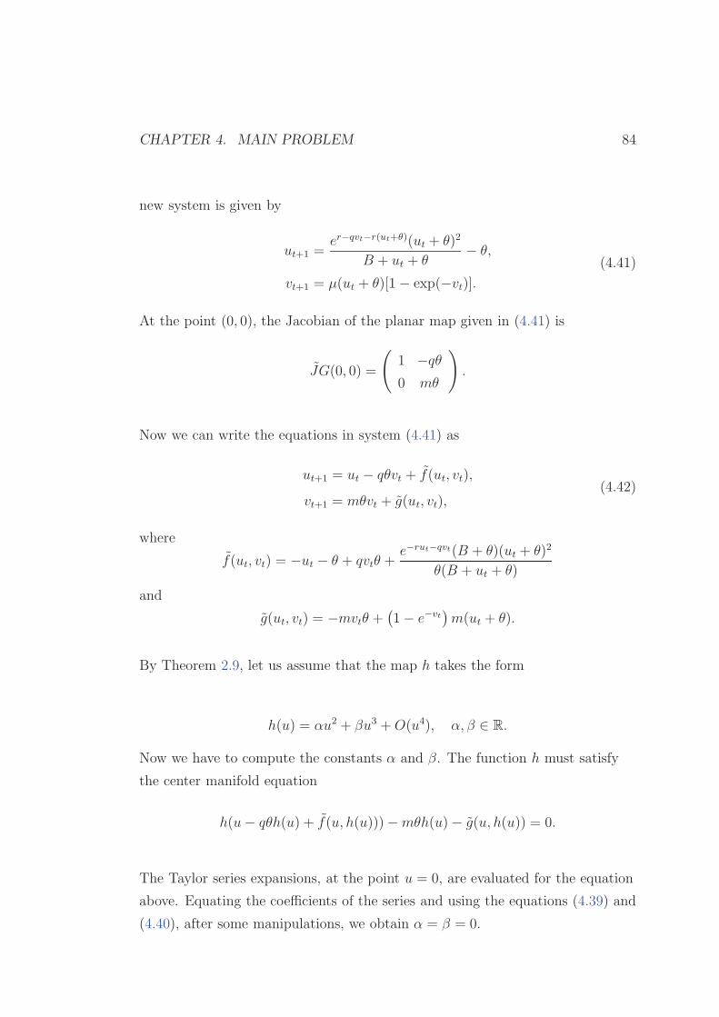
CHAPTER 4. MAIN PROBLEM 84
new system is given by
ut+1 =er−qvt−r(ut+θ)(ut + θ)2
B + ut + θ− θ,
vt+1 = µ(ut + θ)[1− exp(−vt)].(4.41)
At the point (0, 0), the Jacobian of the planar map given in (4.41) is
JG(0, 0) =
(
1 −qθ0 mθ
)
.
Now we can write the equations in system (4.41) as
ut+1 = ut − qθvt + f(ut, vt),
vt+1 = mθvt + g(ut, vt),(4.42)
where
f(ut, vt) = −ut − θ + qvtθ +e−rut−qvt(B + θ)(ut + θ)2
θ(B + ut + θ)
and
g(ut, vt) = −mvtθ +(
1− e−vt)
m(ut + θ).
By Theorem 2.9, let us assume that the map h takes the form
h(u) = αu2 + βu3 +O(u4), α, β ∈ R.
Now we have to compute the constants α and β. The function h must satisfy
the center manifold equation
h(u− qθh(u) + f(u, h(u)))−mθh(u)− g(u, h(u)) = 0.
The Taylor series expansions, at the point u = 0, are evaluated for the equation
above. Equating the coefficients of the series and using the equations (4.39) and
(4.40), after some manipulations, we obtain α = β = 0.
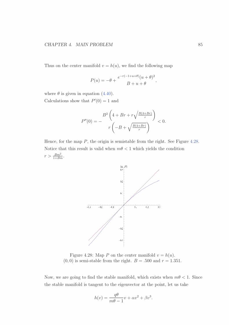
CHAPTER 4. MAIN PROBLEM 85
Thus on the center manifold v = h(u), we find the following map
P (u) = −θ + e−r(−1+u+θ)(u+ θ)2
B + u+ θ,
where θ is given in equation (4.40).
Calculations show that P ′(0) = 1 and
P ′′(0) = −B2
(
4 +Br + r√
B(4+Br)r
)
r
(
−B +√
B(4+Br)r
) < 0.
Hence, for the map P , the origin is semistable from the right. See Figure 4.28.
Notice that this result is valid when mθ < 1 which yields the condition
r > Bm2
1+Bm.
-� � ·
-� �
-� � ¯ � � ¯ � � � � ·
-� � ·-� � -� � ¯� � ¯� � � � ·8¡ ¢ £
<
Figure 4.28: Map P on the center manifold v = h(u).(0, 0) is semi-stable from the right. B = .500 and r = 1.351.
Now, we are going to find the stable manifold, which exists when mθ < 1. Since
the stable manifold is tangent to the eigenvector at the point, let us take
h(v) =qθ
mθ − 1v + αv2 + βv3.
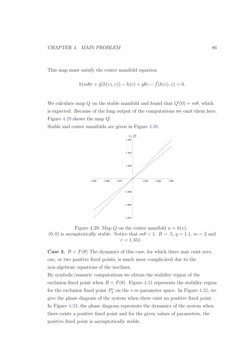
CHAPTER 4. MAIN PROBLEM 86
This map must satisfy the center manifold equation
h(mθv + g(h(v), v))− h(v) + qθv − f(h(v), v) = 0.
We calculate map Q on the stable manifold and found that Q′(0) = mθ, which
is expected. Because of the long output of the computations we omit them here.
Figure 4.29 shows the map Q.
Stable and center manifolds are given in Figure 4.30.
-� � � � ·
-� � � �
-� � � � ¯ � � � � ¯ � � � � � � � � ·
-� � � � ·-� � � � -� � � � ¯� � � � ¯� � � � � � � � ·8¸ ¢ ¹
<
Figure 4.29: Map Q on the center manifold u = h(v).(0, 0) is asymptotically stable. Notice that mθ < 1. B = .5, q = 1.1, m = 2 and
r = 1.351.
Case 3. B < F (θ) The dynamics of this case, for which there may exist zero,
one, or two positive fixed points, is much more complicated due to the
non-algebraic equations of the isoclines.
By symbolic/numeric computations we obtain the stability region of the
exclusion fixed point when B < F (θ). Figure 4.31 represents the stability region
for the exclusion fixed point P ∗3 on the r-m parameter space. In Figure 4.32, we
give the phase diagram of the system when there exist no positive fixed point.
In Figure 4.33, the phase diagram represents the dynamics of the system when
there exists a positive fixed point and for the given values of parameters, the
positive fixed point is asymptotically stable.
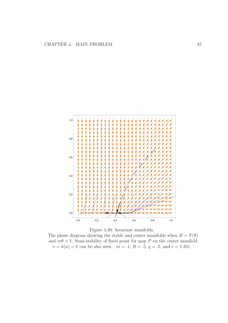
CHAPTER 4. MAIN PROBLEM 87
0.0 0.2 0.4 0.6 0.8 1.0
0.0
0.2
0.4
0.6
0.8
1.0
Figure 4.30: Invariant manifolds.The phase diagram showing the stable and center manifolds when B = F (θ)and mθ < 1. Semi-stability of fixed point for map P on the center manifoldv = h(u) = 0 can be also seen. m = .1, B = .5, q = .5, and r = 1.351.
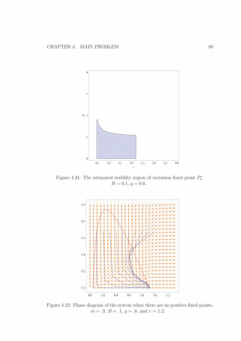
CHAPTER 4. MAIN PROBLEM 88
º » ¼ ½ » º ½ » ¼ ¾ » º ¾ » ¼ ¿ » º ¿ » ¼ À » ºº ½¾¿À
ÁÂ
Figure 4.31: The estimated stability region of exclusion fixed point P ∗3 .B = 0.1, q = 0.6.
º » º º » ¾ º » À º » à º » Ä ½ » º ½ » ¾º » ºº » ¾º » Àº » ú » Ľ » º
Figure 4.32: Phase diagram of the system when there are no positive fixed points.m = .9, B = .1, q = .6, and r = 1.2.
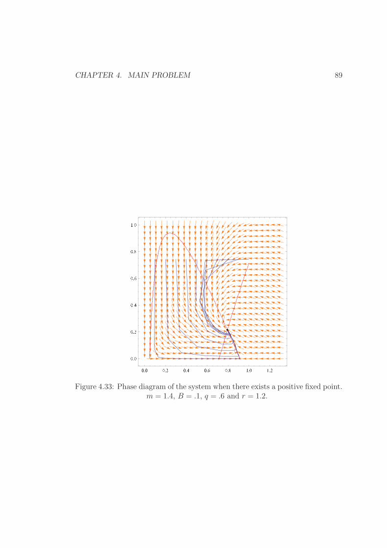
CHAPTER 4. MAIN PROBLEM 89
º » º º » ¾ º » À º » à º » Ä ½ » º ½ » ¾º » ºº » ¾º » Àº » ú » Ľ » º
Figure 4.33: Phase diagram of the system when there exists a positive fixed point.m = 1.4, B = .1, q = .6 and r = 1.2.

Chapter 5
Conclusion and Further Studies
In this thesis, we investigated the stability and bifurcation of a generalized
Beddington host-parasitoid model. We were able to study the stability of the
coexistence fixed point without actually computing it. This is accomplished by
using upper and lower sequences approaching the coexistence fixed point. By
this, we have established the mathematical analysis and provided novel tools to
study the stability of fixed points for the models where there is no explicit
formula for the fixed points. Our results confirmed the known results in the
literature for the special case a = b that were obtained via simulation. The
invariant manifolds for the extinction and exclusion fixed points were obtained.
Due to the lack of an explicit formula of the coexistence fixed point, we were
not able to investigate the Neimark-Sacker bifurcation and the other types of
bifurcations. The presence of Neimark-Sacker bifurcation was shown via
numerical simulations. Moreover, the global dynamics of the system has not
been determined and needs further study.
We also investigated the Beddington model with the parasitoid subject to an
Allee effect and the generalized Beddington model with the host subject to an
Allee effect. We analysed the stability and invariant manifolds of both of the
systems.
90

Appendix A
Mathematica Codes
In Appendix A, we present some of the Mathematica modules used during this
thesis. We wrote and executed the codes on Mathematica 7.0.0. For each
module, we give the code and a simple example of its usage.
A.1 Cobweb Diagram
Code
Cobweb[F_, t0_] :=
Module[{ff, diagonal, funct, list, l, ldot, ttt, sonlist},
ff[a_] := F /. x -> a;
diagonal = Plot[x, {x, 0, 1}, PlotStyle -> Red];
funct = Plot[F, {x, 0, 1}];
list = Table[{Nest[ff, t0, n], Nest[ff, t0, n + 1]}, {n, 0, 100}];
ldot = ListPlot[list];
sonlist = {{t0, 0}};
For[i = 1, i < 101, i++, sonlist = Append[sonlist, list[[i]]];
sonlist =
Append[sonlist, {sonlist[[2 i]][[2]], sonlist[[2 i]][[2]]}]];
91
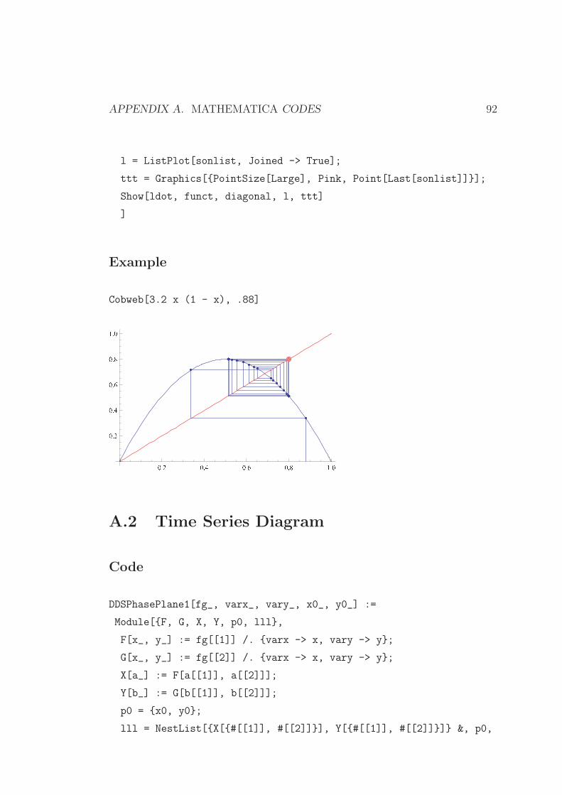
APPENDIX A. MATHEMATICA CODES 92
l = ListPlot[sonlist, Joined -> True];
ttt = Graphics[{PointSize[Large], Pink, Point[Last[sonlist]]}];
Show[ldot, funct, diagonal, l, ttt]
]
Example
Cobweb[3.2 x (1 - x), .88]
º » ¾ º » À º » à º » Ä ½ » ºº » ¾º » Àº » ú » Ľ » º
A.2 Time Series Diagram
Code
DDSPhasePlane1[fg_, varx_, vary_, x0_, y0_] :=
Module[{F, G, X, Y, p0, lll},
F[x_, y_] := fg[[1]] /. {varx -> x, vary -> y};
G[x_, y_] := fg[[2]] /. {varx -> x, vary -> y};
X[a_] := F[a[[1]], a[[2]]];
Y[b_] := G[b[[1]], b[[2]]];
p0 = {x0, y0};
lll = NestList[{X[{#[[1]], #[[2]]}], Y[{#[[1]], #[[2]]}]} &, p0,
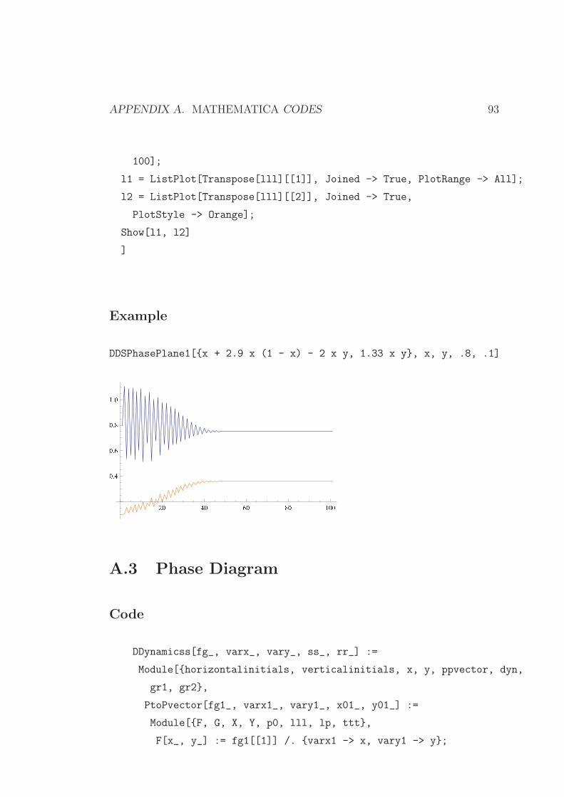
APPENDIX A. MATHEMATICA CODES 93
100];
l1 = ListPlot[Transpose[lll][[1]], Joined -> True, PlotRange -> All];
l2 = ListPlot[Transpose[lll][[2]], Joined -> True,
PlotStyle -> Orange];
Show[l1, l2]
]
Example
DDSPhasePlane1[{x + 2.9 x (1 - x) - 2 x y, 1.33 x y}, x, y, .8, .1]
¾ º À º à º Ä º ½ º ºº » Àº » ú » Ľ » º
A.3 Phase Diagram
Code
DDynamicss[fg_, varx_, vary_, ss_, rr_] :=
Module[{horizontalinitials, verticalinitials, x, y, ppvector, dyn,
gr1, gr2},
PtoPvector[fg1_, varx1_, vary1_, x01_, y01_] :=
Module[{F, G, X, Y, p0, lll, lp, ttt},
F[x_, y_] := fg1[[1]] /. {varx1 -> x, vary1 -> y};
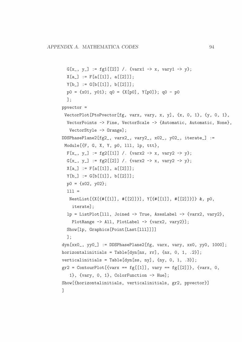
APPENDIX A. MATHEMATICA CODES 94
G[x_, y_] := fg1[[2]] /. {varx1 -> x, vary1 -> y};
X[a_] := F[a[[1]], a[[2]]];
Y[b_] := G[b[[1]], b[[2]]];
p0 = {x01, y01}; q0 = {X[p0], Y[p0]}; q0 - p0
];
ppvector =
VectorPlot[PtoPvector[fg, varx, vary, x, y], {x, 0, 1}, {y, 0, 1},
VectorPoints -> Fine, VectorScale -> {Automatic, Automatic, None},
VectorStyle -> Orange];
DDSPhasePlane2[fg2_, varx2_, vary2_, x02_, y02_, iterate_] :=
Module[{F, G, X, Y, p0, lll, lp, ttt},
F[x_, y_] := fg2[[1]] /. {varx2 -> x, vary2 -> y};
G[x_, y_] := fg2[[2]] /. {varx2 -> x, vary2 -> y};
X[a_] := F[a[[1]], a[[2]]];
Y[b_] := G[b[[1]], b[[2]]];
p0 = {x02, y02};
lll =
NestList[{X[{#[[1]], #[[2]]}], Y[{#[[1]], #[[2]]}]} &, p0,
iterate];
lp = ListPlot[lll, Joined -> True, AxesLabel -> {varx2, vary2},
PlotRange -> All, PlotLabel -> {varx2, vary2}];
Show[lp, Graphics[Point[Last[lll]]]]
];
dyn[xx0_, yy0_] := DDSPhasePlane2[fg, varx, vary, xx0, yy0, 1000];
horizontalinitials = Table[dyn[nx, rr], {nx, 0, 1, .2}];
verticalinitials = Table[dyn[ss, ny], {ny, 0, 1, .3}];
gr2 = ContourPlot[{varx == fg[[1]], vary == fg[[2]]}, {varx, 0,
1}, {vary, 0, 1}, ColorFunction -> Hue];
Show[{horizontalinitials, verticalinitials, gr2, ppvector}]
]
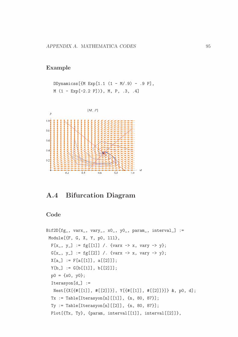
APPENDIX A. MATHEMATICA CODES 95
Example
DDynamicss[{M Exp[1.1 (1 - M/.9) - .9 P],
M (1 - Exp[-2.2 P])}, M, P, .3, .4]
º » ¾ º » À º » à º » Ä ½ » º ź » ¾º » Àº » ú » Ľ » º Æ 8Ç È É
<
A.4 Bifurcation Diagram
Code
Bif2D[fg_, varx_, vary_, x0_, y0_, param_, interval_] :=
Module[{F, G, X, Y, p0, lll},
F[x_, y_] := fg[[1]] /. {varx -> x, vary -> y};
G[x_, y_] := fg[[2]] /. {varx -> x, vary -> y};
X[a_] := F[a[[1]], a[[2]]];
Y[b_] := G[b[[1]], b[[2]]];
p0 = {x0, y0};
Iterasyon[d_] :=
Nest[{X[{#[[1]], #[[2]]}], Y[{#[[1]], #[[2]]}]} &, p0, d];
Tx := Table[Iterasyon[n][[1]], {n, 80, 87}];
Ty := Table[Iterasyon[n][[2]], {n, 80, 87}];
Plot[{Tx, Ty}, {param, interval[[1]], interval[[2]]},
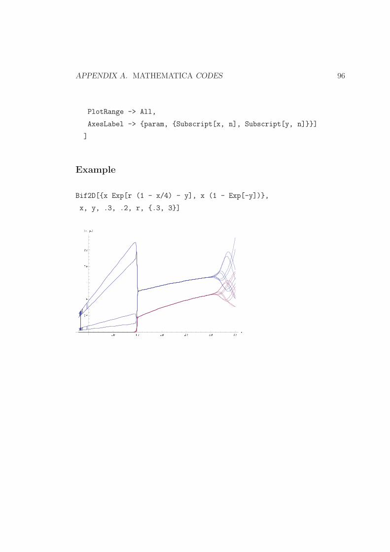
APPENDIX A. MATHEMATICA CODES 96
PlotRange -> All,
AxesLabel -> {param, {Subscript[x, n], Subscript[y, n]}}]
]
Example
Bif2D[{x Exp[r (1 - x/4) - y], x (1 - Exp[-y])},
x, y, .3, .2, r, {.3, 3}]
Ê Ë Ì Ê Ë Í Î Ë Ì Î Ë Í Ï Ë Ì Ï Ë Í ÐÌ Ë ÍÊ Ë ÌÊ Ë ÍÎ Ë ÌÎ Ë Í8Ñ Ò Ó Ô Ò<

Appendix B
Stability of Fixed Points
In this section, we present the behaviour of a linear system determined by the
eigenvalues and trace-determinant of the Jacobian matrix.
97
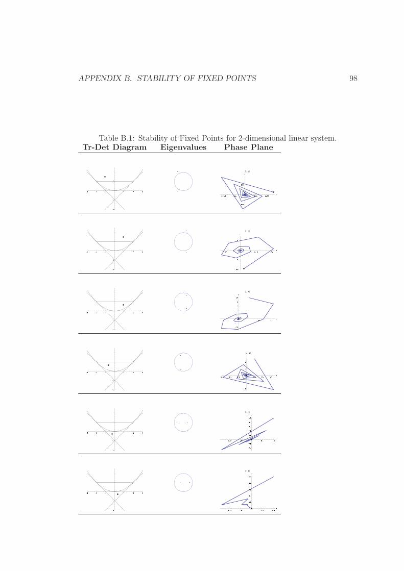
APPENDIX B. STABILITY OF FIXED POINTS 98
Table B.1: Stability of Fixed Points for 2-dimensional linear system.Tr-Det Diagram Eigenvalues Phase Plane
-Õ
-Ö
-× × Ö Õ
-Ö-××Ö -
× Ø Ø Ø Ø-
Ù Ø Ø Ø Ù Ø Ø Ø × Ø Ø Ø Ø Ú-
Ù Ø Ø ØÙ Ø Ø Ø Û 8Ü Ý Þ <-
Õ-
Ö-
× × Ö Õ-
Ö-××Ö -Ù Ø Ø Ø Ù Ø Ø Ø × Ø Ø Ø Ø Ú
-× Ø Ø Ø Ø-
Ù Ø Ø ØÙ Ø Ø Ø Û 8Ü Ý Þ<
-Õ
-Ö
-× × Ö Õ
-Ö-××Ö
-Ø ß × Ø ß × Ø ß Ö Ø ß Õ Ú
-Ø ß Ö-Ø ß ×Ø ß ×Ø ß ÖØ ß ÕØ ß àØ ß Ù Û 8
Ü Ý Þ<
-Õ
-Ö
-× × Ö Õ
-Ö-××Ö -
Ø ß Õ-
Ø ß Ö-
Ø ß × Ø ß × Ø ß Ö Ø ß Õ Ú-
Ø ß à-Ø ß ÖØ ß ÖØ ß à Û8Ü Ý Þ<
-Õ
-Ö
-× × Ö Õ
-Ö-××Ö
-Ø ß × Ø
-Ø ß Ø Ù Ø ß Ø Ù Ø ß × Ø Ú
-Ø ß Ö-Ø ß ×Ø ß ×Ø ß ÖØ ß ÕØ ß àØ ß Ù Û8
Ü Ý Þ<
-Õ
-Ö
-× × Ö Õ
-Ö-××Ö
-Ø ß × Ø
-Ø ß Ø Ù Ø ß Ø Ù Ø ß × Ø ÚØ ß ×Ø ß ÖØ ß ÕØ ß àØ ß Ù Û8Ü Ý Þ <
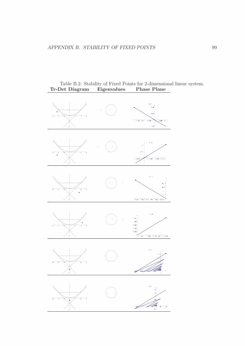
APPENDIX B. STABILITY OF FIXED POINTS 99
Table B.2: Stability of Fixed Points for 2-dimensional linear system.Tr-Det Diagram Eigenvalues Phase Plane
-Õ
-Ö
-× × Ö Õ
-Ö-××Ö
-Õ × Ø á â
-Ö × Ø á â
-× × Ø á â × × Ø á â Ö × Ø á â Ú
-Ù × Ø á âÙ × Ø á â× × Ø á ã Û8Ü Ý Þ <
-Õ
-Ö
-× × Ö Õ
-Ö-××Ö
-× ß Ø × Ø á ä
-Ù ß Ø × Ø á å Ù ß Ø × Ø á å × ß Ø × Ø á ä × ß Ù × Ø á ä Ö ß Ø × Ø á ä Ö ß Ù × Ø á ä ÚÙ × Ø á ä× × Ø á æ Û
8Ü Ý Þ <-
Õ-
Ö-
× × Ö Õ-
Ö-××Ö-
Õ ß Ù × Ø á ç-
Õ ß Ø × Ø á ç-
Ö ß Ù × Ø á ç-
Ö ß Ø × Ø á ç-
× ß Ù × Ø á ç-
× ß Ø × Ø á ç-
Ù ß Ø × Ø á ã ÚÖ × Ø á çà × Ø á çè × Ø á çé × Ø á ç Û8Ü Ý Þ<
-Õ
-Ö
-× × Ö Õ
-Ö-××Ö Ù ß Ø × Ø á á × ß Ø × Ø á â × ß Ù × Ø á â Ö ß Ø × Ø á â Ö ß Ù × Ø á âÚÖ × Ø á âà × Ø á âè × Ø á âé × Ø á â× × Ø á ã Û 8
Ü Ý Þ<
-Õ
-Ö
-× × Ö Õ
-Ö-××Ö
-Ö Ø Ø Ø Ø
-× Ù Ø Ø Ø
-× Ø Ø Ø Ø
-Ù Ø Ø Ø ÚÙ Ø Ø Ø× Ø Ø Ø Ø× Ù Ø Ø ØÖ Ø Ø Ø Ø Û8Ü Ý Þ <
-Õ
-Ö
-× × Ö Õ
-Ö-××Ö
-Ø ß Ö Ø
-Ø ß × Ù
-Ø ß × Ø
-Ø ß Ø Ù Ø ß Ø Ù Ø ß × Ø Ú
-Ø ß ×Ø ß ×Ø ß ÖØ ß ÕØ ß àØ ß Ù Û8
Ü Ý Þ<

APPENDIX B. STABILITY OF FIXED POINTS 100
Table B.3: Stability of Fixed Points for 2-dimensional linear system.Tr-Det Diagram Eigenvalues Phase Plane
-Õ
-Ö
-× × Ö Õ
-Ö-××Ö
-Ø ß × Ø
-Ø ß Ø Ù Ø ß Ø Ù Ø ß × Ø Ø ß × Ù Ø ß Ö Ø Ú
-Ø ß Ö-Ø ß ×Ø ß ×Ø ß ÖØ ß ÕØ ß àØ ß Ù Û 8
Ü Ý Þ<
-Õ
-Ö
-× × Ö Õ
-Ö-××Ö -
Ù Ø Ø Ø Ù Ø Ø Ø Ú-
× Ø Ø Ø Ø-Ù Ø Ø ØÙ Ø Ø Ø Û 8
Ü Ý Þ<
-Õ
-Ö
-× × Ö Õ
-Ö-××Ö -
Ø ß è-
Ø ß à-
Ø ß Ö Ø ß Ö Ø ß à Ø ß è Ú-
Ø ß è-Ø ß à-Ø ß ÖØ ß ÖØ ß àØ ß è Û8Ü Ý Þ <-
Õ-
Ö-
× × Ö Õ-
Ö-××Ö -Ø ß à
-Ø ß Ö Ø ß Ö Ø ß à Ú
-Ø ß à-Ø ß ÖØ ß ÖØ ß à Û8Ü Ý Þ
<
-Õ
-Ö
-× × Ö Õ
-Ö-××Ö -
Ø ß Ö-
Ø ß × Ø ß × Ø ß Ö Ú-
Ø ß à-Ø ß ÖØ ß ÖØ ß à Û8Ü Ý Þ<
-Õ
-Ö
-× × Ö Õ
-Ö-××Ö
-Ø ß Ö Ù
-Ø ß Ö Ø
-Ø ß × Ù
-Ø ß × Ø
-Ø ß Ø Ù Ø ß Ø Ù Ø ß × Ø ÚØ ß Ö ØØ ß Ö ÙØ ß Õ ØØ ß Õ ÙØ ß à ØØ ß à ÙØ ß Ù Ø Û8Ü Ý Þ <

BIBLIOGRAPHY
[1] W.C. Allee, Animal aggregation, a study in general sociology, University of
Chicago Press, Chicago, USA, 1931.
[2] W.C. Allee, The Social Life of Animal, William Heinemann, 1938.
[3] L. Allen, An introduction to mathematical biology, Prentice Hall, 2007.
[4] J.R. Beddington, C.A. Free, and J.H. Lawton, Dynamic complexity in
predator-prey models framed in difference equations, Nature 225 (1975),
58–60.
[5] R. J. H. Beverton and S. J. Holt, On the dynamics of exploited fish
populations, vol. 19, Chapman and Hall, 1957.
[6] X. Cabre, E. Fontich, and R. de la Llave, The parameterization method for
invariant manifolds i: Manifolds associated to non-resonant subspaces,
Indiana Univ.Math. J. 52 (2003), 283–328.
[7] J. Carr, Application of center manifolds theory, Applied Mathematical
Sciences, Springer-Verlag, New York, 1981.
[8] H. Caswell, Matrix population models: construction, analysis, and
interpretation, vol. 2nd, Sinauer Associates, 2001.
[9] F. Courchamp, L. Berec, and J. Gascoigne, Allee effects in ecology and
conservation, Oxford University Press, 2008.
[10] C. Celik, O. Duman, Allee effect in a discrete-time predator-prey system,
Chaos, Solitons and Fractals 40, (2009) 1956-1962.
101
BIBLIOGRAPHY 102
[11] M.G. Neubert and M. Kot, The subcritical collapse of predator populations
in discrete-time predator-prey models, Mathematical Biosciences, 110,
(1992), 45–66, ISSN 0025-5564, 10.1016/0025-5564(92)90014-N.
[12] S. Elaydi, An introduction to difference equations, Springer, 2000.
[13] S. Elaydi, Discrete chaos: With applications in science and engineering,
second edition, Chapman & Hall/CRC, 2008.
[14] S. Elaydi and R.J. Sacker, Population models with allee effect: a new
model, Journal of Biological Dynamics 4 (2010), no. 4, 397–408.
[15] S. Elaydi and R. Sacker, Basin of Attraction of Periodic Orbits of Maps on
the Real Line, Journal of Difference Equations and Applications , (2004),
10, Iss. 10.
[16] S.A. Geritz and E. Kisdi, On the mechanistic underpinning of discrete-time
population models with complex dynamics, J Theor Biol. (2004), no. 228,
261–9.
[17] P.H. Leslie and J. C. Gower, The properties of a stochastic model for the
predator-prey type of interaction between two species, Biometrika, V 47,
3/4, p. 219, 1960.
[18] M. Guzowska, R. Luis, and S. Elaydi, Bifurcation and invariant manifolds
of the logistic competition model, Journal of Difference Equations and
Applications 17 (2010), no. 12, 1851–1872.
[19] J. Hofbauer and K. Sigmund, Evolutionary games and population
dynamics, Cambridge University Press, Cambridge New York, NY, 1998.
[20] R.A. Holmgren, A first course in discrete dynamical systems,
Springer-Verlag, New York, 1994.
[21] A.N.W Hone, M.V. Irle, and G.W. Thurura, On the neimark–sacker
bifurcation in a discrete predator-prey system, Journal of Biological
Dynamics 4 (2010), no. 6, 594–606.
BIBLIOGRAPHY 103
[22] S.R.-J. Jang and S.L. Diamond, A host-parasitoid interaction with allee
effects on the host, Computers and Mathematics with Applications 53
(2007), 89–103.
[23] N. Karydas and J. Schinas, The center manifold theorem for a discrete
system, Appl. Anal. 44 (1992), 267–284.
[24] P.A. Stephens, W.J. Sutherland, and R.P. Freckleton, What is the Allee
Effect, Oikos 87 (1999), 185-90.
[25] P.A. Stephens and W.J. Sutherland, Vertebrate mating systems, Allee
effects and conservation. In M. Apollonio, M. Festa-Bianchet and D.
Mainardi, eds. Vertebrate mating systems, pp. 186-213, World Scientific
Publishing, Singapore, 2000.
[26] D. Clark and M. R. S. Kulenovik, On a coupled system of rational
difference equations, Comput. Math. Appl.,(2002)
[27] M. P. Hassell and H. N. Comins, Discrete time models for two-species
competition, Theor: Popul.Biol., 9, (1976), 202-221
[28] M.R.S. Kulenovic and M. Nurkanovic, Global Asymptotic Behavior of a
Two-dimensional System of Difference Equations Modeling Cooperation,
Journal of Difference Equations and Applications,2003 VOL. 9 (1). pp.
149-159
[29] J. C. Misra and A. Mitra, Instabilities in Single-Species and Host-Parasite
Systems:Period-Doubling Bifurcations and Chaos, An Int. Jour. Computer
and Graphics with Applications, 52, (2005), 525-538
[30] J. F. Selgrade and M. Ziehe, Convergence to equilibrium in a genetic model
with differential viability between the sexes, J. Math. Eiol., 25 (1987),
477-490.
[31] H. L. Smith, Monotone Dynamical Systems: An introduction to the Theory
of Competitive and Cooperative Systems, American Mathematical Society,
Providence, 1995.
BIBLIOGRAPHY 104
[32] A. Kelly, The stable, center-stable, center-unstable and unstable manifolds,
J. Differential Equ. 3 (1967).
[33] M. Kot, M. A. Lewis, and P. Van Den Driessche, Dispersal data and the
spread of invading organisms, Ecology 77 (1996), no. 7, 2027–2042.
[34] A.M. Kramer, B. Dennis, A.M. Liebhold, and J.M. Drake, The evidence for
allee effects, Population Ecology 51 (2009), no. 3, 341–354 (English).
[35] Y.A. Kuznetsov, Elements of applied bifurcation theory, Springer, New
York, 1998.
[36] M.A. Lewis and P. Kareiva, Allee dynamics and the spread of invading
organisms, Theoretical Population Biology 43 (1993), no. 2, 141 – 158.
[37] G. Livadiotis and S. Elaydi, General allee effect in two-species population
biology, Journal of Biological Dynamics 6 (2012), no. 2, 959–973, PMID:
22881395.
[38] A.J. Lotka, Elements of physical biology, Baltimore: Williams and Wilkins,
1925.
[39] R. Luıs, S. Elaydi, and S. Oliveira, Stability of ricker-type competition
model and the competitive exclusion principle, Journal of Biological
Dynamics 5 (2011), 636–660.
[40] J. Marsden and M. McCracken, The hopf bifurcation and its application,
Springer-Verlag, New York, 1976.
[41] R. M. May, Limit cycles in predator-prey communities., Science 177
(1972), no. 4052, 900–902.
[42] J. D. Murray, Mathematical biology, Springer, New York, 2002.
[43] Ju.I. Neimark, On some cases of periodic motions depending on
parameters., Dokl. Akad. Nauk SSSR (1959), 129, 736–739 [in Russian].
[44] A. Nicholson and V. Bailey, The balance of animal population, Proceedings
of the Zoological Society of London 3 (1935), 551–598.
BIBLIOGRAPHY 105
[45] W. E. Ricker, Stock and recruitment, Journal of the Fisheries Research
Board of Canada 11 (1954), no. 5, 559–623.
[46] R. Sacker, On invariant surfaces and bifurcation of periodic solutions of
ordinary differential equations, Report IMM-NYU 333 (1964),New York
University.
[47] E. Scheinerman, Invitation to dynamical systems, Prentice Hall, Upper
Saddle River, N.J, 1996.
[48] P. Turchin, Complex population dynamics : a theoretical/empirical
synthesis, Princeton University Press, Princeton, N.J, 2003.
[49] U. Ufuktepe and S. Kapcak, Stability analysis of a host parasite model,
Advances in Difference Equations 79 (2013),
doi:10.1186/1687-1847-2013-79.
[50] Volterra V., Fluctuations in the abundance of a species, Nature 118 (1924),
558–560.
[51] A. Vanderbauwhede, Center manifolds, normal forms and elementary
bifurcations, Dynamics Reported, 1989.
[52] W-X. Wang, Y. Zhang, and C. Liu, Analysis of a discrete-time
predator-prey system with allee effect, Ecological Complexity 8 (2011),
81–85.
[53] S. Wiggins, Introduction to applied nonlinear dynamical systems and chaos,
Springer, New York, 2003.
[54] S-R. Zhou, Y-F. Liu, and G. Wang, The stability of predator-prey systems
subject to the allee effects, Theoretical Population Biology 67 (2005), no. 1,
23–31.

BIBLIOGRAPHY 106
VITA
Sinan Kapcak was born in 1978 in Diyarbakır, Turkey.
He graduated from Akdeniz University in 2001 with a degree in Mathematics.
He received his Masters of Mathematics degree from Izmir Institute of
Technology in 2007. He spent his 2006-2007 Fall semester at the University of
Cantabria, Spain, Department of Applied Mathematics and Computational
Science, studying on Petri Nets. With a Ph.D. research grant from TUBITAK,
he studied on Discrete Dynamical Systems and Mathematical Modelling at
Trinity University, USA, in the second half of 2012, under the supervision of his
co-supervisor Prof. Dr. Saber Elaydi.
He completed the requirements for the Doctor of Philosophy degree in the
Graduate Program of Applied Mathematics and Statistics at Izmir University of
Economics under the supervision of Prof. Dr. Unal Ufuktepe and Prof. Dr.
Saber Elaydi. His research interests include Dynamical Systems and
Biomathematics.