Digital Object Identifier (DOI):10.1007/s002850100079

J. Math. Biol. 42, 489–506 (2001) Mathematical Biology

Sze-Bi Hsu · Tzy-Wei Hwang · Yang Kuang

Global analysis of the Michaelis–Menten-typeratio-dependent predator-prey system

Received: 15 January 2000 / Revised version: 7 November 2000Published online: 10 April 2001 – c© Springer-Verlag 2001

Abstract. The recent broad interest on ratio-dependent based predator functional responsecalls for detailed qualitative study on ratio-dependent predator-prey differential systems. Afirst such attempt is documented in the recent work of Kuang and Beretta(1998), whereMichaelis-Menten-type ratio-dependent model is studied systematically. Their paper, whilecontains many new and significant results, is far from complete in answering the many subtlemathematical questions on the global qualitative behavior of solutions of the model. Indeed,many of such important open questions are mentioned in the discussion section of theirpaper.

Through a simple change of variable, we transform the Michaelis-Menten-type ratio-dependent model to a better studied Gause-type predator-prey system. As a result, we canobtain a complete classification of the asymptotic behavior of the solutions of the Michaelis-Menten-type ratio-dependent model. In some cases we can determine how the outcomesdepend on the initial conditions. In particular, open questions on the global stability ofall equilibria in various cases and the uniqueness of limit cycles are resolved. Biologicalimplications of our results are also presented.

1. Introduction

One of the most popular mathematical model describing a predator-prey interac-tion is the following well-known Lotka-Volterra type predator-prey model withMichaelis-Menten (or Holling type II) functional response (Freedman (1980), May(1974)):

x′(t) = ax(1 − x/K) − cxy/(m + x)

y′(t) = y(f x/(m + x) − d)

x(0) > 0, y(0) > 0(1.1)

S.-B. Hsu: Department of Mathematics, National Tsing Hua University, Hsinchu, Taiwan,R.O.C. Research supported by National Council of Science, Republic of China

T.-W. Hwang: Department of Mathematics, Kaohsiung Normal University, 802, Kaohsiung,Taiwan, R.O.C. Research supported by National Council of Science, Republic of China

Y. Kuang: Department of Mathematics, Arizona State University, Tempe, AZ 85287-1804,USA. e-mail: kuang@asu.edu. Work is partially supported by NSF grant DMS-0077790 and is initiated while visiting the National Center for Theoretical Science, TsingHua University, Hsinchu, Taiwan R.O.C.

Key words or phrases: Ratio-dependent predator-prey model – Global stability – Uniquenessof limit cycles – Extinction

Mathematics Subject Classification (2000): 34D05, 34D20, 92D25

490 S.-B. Hsu et al.

wherex, y stand for prey and predator density, respectively.a,K, c,m, f, d are pos-itive constants that stand for prey intrinsic growth rate, carrying capacity, capturingrate, half saturation constant, maximal predator growth rate, predator death rate,respectively. This model exhibit the well-known “paradox of enrichment" observedby Hairston et al. (1960) and by Rosenzweig (1969) which states that accordingto model (1.1), enriching a predator-prey system (increasing the carrying capacityK) will cause an increase in the equilibrium density of the predator but not in thatof the prey, and will destabilize the positive equilibrium (the positive steady statechanges from stable to unstable as K increases). An equivalent paradox is the socalled “biological control paradox” which was recently brought into discussion byLuck (1990), stating that according to (1.1), we cannot have both a low and stableprey equilibrium density. However, in reality, there are numerous examples of suc-cessful biological control where the prey are maintained at densities less than 2% oftheir carrying capacities (Arditi and Berryman (1991)). This clearly indicates thatthe paradox of biological control is not intrinsic to predator-prey interactions. An-other noteworthy prediction from model (1.1) is that prey and predator species cannot extinct simultaneously (mutual extinction). This, however, clearly contradictsGause’s classic observation of mutual extinction in the protozoans, Parameciumand its predator Didinium (Gause (1934), Abrams and Ginzburg (2000)).

Recently there is a growing evidences (Arditi et al. (1991), Akcakaya et al.(1995), Cosner et al. (1999)) that in some situations, especially when predator haveto search for food (and therefore have to share or compete for food), a more suitablegeneral predator-prey theory should be based on the so called ratio-dependent the-ory, which can be roughly stated as that the per capita predator growth rate shouldbe a function of the ratio of prey to predator abundance. This is supported bynumerous field and laboratory experiments and observations (Arditi and Ginzburg(1989), Arditi et al. (1991)). Generally, a ratio-dependent predator-prey model takesthe form

x′(t) = xf (x) − yp(x/y)

y′(t) = (cq(x/y) − d)y.

Here p(x) is the so-called predator functional response. Often, q(x) is replaced byp(x), in which case c becomes the conversion rate. p(x), q(x) satisfy the usualproperties such as being nonnegative and increasing, and equal to zero at zero.

Geometrically, the differences of prey-dependent and ratio-dependent modelsare obvious, the former has a vertical predator isocline, while the latter has a slantedone. There are even more differences in their prey isoclines. Local stability analysisand simulations (Arditi and Ginzburg (1989), Berryman (1992)) show that the ratio-dependent models are capable of producing richer and more reasonable dynamicsbiologically. Specifically, it will not produce the paradox of biological control andthe so-called paradox of enrichment. It also allows mutual extinction as a possibleoutcome of a given predator-prey interaction (Kuang and Beretta (1998), Jost et al.(1999)).

In this paper we study following ratio-dependent predator-prey system whichwas discussed in Kuang and Beretta (1998) (see also Jost et al. (1999)):

Ratio-dependent predator-prey model 491

x′(t) = ax(1 − x/K) − cxy/(my + x) ≡ F(x, y),

y′(t) = y(−d + f x/(my + x)) ≡ G(x, y),

x(0) = x0 > 0, y(0) = y0 > 0(1.2)

where a,K, c,m, f, d are positive constants and x(t), y(t) represent the populationdensity of prey and predator at time t respectively. The prey grows with intrinsicgrowth rate a and carrying capacity K in the absence of predation. The predatorconsumes the prey with functional response of Michaelis-Menten type cuy/(m +u), u = x/y and contributes to its growth with rate f uy/(m + u). The constant dis the death rate of predator. Observe that lim(x,y)→(0,0) F (x, y) = G(x, y) = 0.We thus define that F(0, 0) = G(0, 0) = 0. Clearly, with this assumption, both F

and G are continuous on the closure of R2+ where R2+ = {(u, y)| u > 0, y > 0}.Kuang and Beretta (1998) presented some global qualitative analysis of so-

lutions of system (1.2). The authors showed that ratio-dependent predator-preymodels are rich in boundary dynamics. For example, for some initial conditions,both predator and prey can go extinction simultaneously. They also established thatthe system has no nontrivial periodic solutions provided the positive steady stateis locally asymptotic stable. Similar results for more general Gause-type ratio-dependent predator-prey systems can be found in Kuang (1999).

For simplicity, we nondimensionalizes the system (1.2) as in Kuang and Beretta(1998) with the following scaling

t→at, x→x/K, y→my/K

then the system (1.2) takes the form

x′(t) = x(1 − x) − sxy/(x + y),

y′(t) = δy(−r + x/(x + y)),

x(0) = x0 > 0, y(0) = y0 > 0,(1.3)

where

s = c

ma, δ = f

a, r = d

f. (1.4)

Results of Kuang and Beretta (1998) and their open questions are summarized intable 1.

In this paper we shall give an almost complete classification for the asymptoticbehavior of the solutions of (1.3). The open questions proposed by Kuang andBeretta in (1998) are all answered here. When relevant, it is determined how theoutcomes depends on the initial conditions. We also establish the uniqueness oflimit cycles if it exists.

The rest of this paper is organized as follows. In section 2, by a simple but crucialchange of variables, we transform the system (1.3) into a Gause-type predator-preysystem (2.1) where a wealth of existing methods and results are applicable. We thusobtain a better understanding of the rich asymptotic behavior of the solutions ofthe system (1.3) through that of system (2.1). Section 3 presents direct biologicalimplications of all our mathematical results in terms of the original parameters insystem (1.2).

492 S.-B. Hsu et al.

Table 1. Established results and open questions of Kuang and Beretta (1998) in terms ofs, δ, r .

Conditions Results or question

1. r ≥ 1, s > 0, (1, 0) is locally asymptotically stable.

2. r ≥ 1, 0 < s ≤ 1, (1, 0) is globally asymptotically stable.

3. s > 1 + δr , There exists (x(t), y(t))→(0, 0). as t→∞Hence, the system is not persistent.

4. r ≥ 1, 1 < s ≤ 1 + δr , (1, 0) is locally stable.

OPEN QUESTION 1: Is (1, 0) globally stable?

5. 0 < r < 1, 0 < s ≤ 1, E∗ is globally stable.

6. 0 < r < 1, s > 11−r

, (0, 0) is globally stable.

7. 0 < r < 1, 1 < s < 11−r

E∗ is locally stable.

δ(1 − r) ≥ 1 OPEN QUESTION 2: Is E∗ globally stable?

8. 0 < r < 1, 1 < s < 11−r

(i) OPEN QUESTION 3: Is it true that if 1 < s ≤ 1 + δr ,

δ(1 − r) < 1 then E∗ is globally stable?

(ii) If 1 + δr < s < 11−r2 + rδ

1+r, E∗ is locally.

stable and the system is not persistent.

(iii) 11−r2 + rδ

1+r< s < 1

1−rthen E∗ is unstable.

and the system is not persistent.

2. Main results

We make the change of variable (x, y) → (u, y) where u = x/y in system (1.3).This reduces it to the following Gause-type predator-prey system (2.1)

u′(t) = g(u) − ϕ(u)y,

y′(t) = ψ(u)y,

u(0) = u0 > 0, y(0) = y0 > 0(2.1)

whereg(u) = u(1 + δr − s + (1 + δr − δ)u)/(1 + u),

ϕ(u) = u2

ψ(u) = δ(u/(u + 1) − r).

(2.2)

Since (2.1) can also be rewritten as

u′(t) = ϕ(u)(h(u) − y),

y′(t) = ψ(u)y,(2.3)

we see that the prey isocline of the system (2.1) is given by

y = g(u)

ϕ(u)= h(u) = (1 + δr − s + (1 + δr − δ)u)/u(u + 1). (2.4)

Ratio-dependent predator-prey model 493

Clearly, limu→+∞ h(u) = 0 and

h′(u) = −[(1 + δr − δ)u2 + 2(1 + δr − s)u + (1 + δr − s)]/u2(1 + u)2. (2.5)

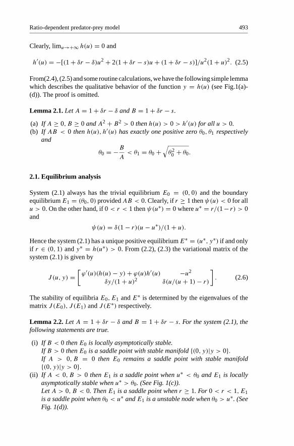
From(2.4), (2.5) and some routine calculations, we have the following simple lemmawhich describes the qualitative behavior of the function y = h(u) (see Fig.1(a)-(d)). The proof is omitted.

Lemma 2.1. Let A = 1 + δr − δ and B = 1 + δr − s.

(a) If A ≥ 0, B ≥ 0 and A2 + B2 > 0 then h(u) > 0 > h′(u) for all u > 0.(b) If AB < 0 then h(u), h′(u) has exactly one positive zero θ0, θ1 respectively

and

θ0 = −B

A< θ1 = θ0 +

√θ2

0 + θ0.

2.1. Equilibrium analysis

System (2.1) always has the trivial equilibrium E0 = (0, 0) and the boundaryequilibrium E1 = (θ0, 0) provided AB < 0. Clearly, if r ≥ 1 then ψ(u) < 0 for allu > 0. On the other hand, if 0 < r < 1 then ψ(u∗) = 0 where u∗ = r/(1 − r) > 0and

ψ(u) = δ(1 − r)(u − u∗)/(1 + u).

Hence the system (2.1) has a unique positive equilibrium E∗ = (u∗, y∗) if and onlyif r ∈ (0, 1) and y∗ = h(u∗) > 0. From (2.2), (2.3) the variational matrix of thesystem (2.1) is given by

J (u, y) =[ϕ′(u)(h(u) − y) + ϕ(u)h′(u) −u2

δy/(1 + u)2 δ(u/(u + 1) − r)

]. (2.6)

The stability of equilibria E0, E1 and E∗ is determined by the eigenvalues of thematrix J (E0), J (E1) and J (E∗) respectively.

Lemma 2.2. Let A = 1 + δr − δ and B = 1 + δr − s. For the system (2.1), thefollowing statements are true.

(i) If B < 0 then E0 is locally asymptotically stable.If B > 0 then E0 is a saddle point with stable manifold {(0, y)|y > 0}.If A > 0, B = 0 then E0 remains a saddle point with stable manifold{(0, y)|y > 0}.

(ii) If A < 0, B > 0 then E1 is a saddle point when u∗ < θ0 and E1 is locallyasymptotically stable when u∗ > θ0. (See Fig. 1(c)).Let A > 0, B < 0. Then E1 is a saddle point when r ≥ 1. For 0 < r < 1, E1is a saddle point when θ0 < u∗ and E1 is a unstable node when θ0 > u∗. (SeeFig. 1(d)).

494 S.-B. Hsu et al.

(iii) If A < 0, B > 0 then E∗ is locally asymptotically stable when u∗ < θ0. (SeeFig. 1(c)).If A > 0, B < 0 then E∗ is a unstable focus or node if θ0 < u∗ < θ1 and E∗is asymptotically stable if u∗ > θ1.If A ≥ 0, B > 0 then E∗ is asymptotically stable. (See Fig. 1(a)).

Proof. From(2.6) and (2.4), (2.5), the variational matrix of the system (2.1) at E0 is

J (E0) =[

1 + δr − s 00 −δr

].

Obviously the first two cases of (i) hold. The last case of (i) can be seen directlyfrom the system (2.1).

For part(ii), the variational matrix at E1 is

J (E1) =[ϕ(θ0)h

′(θ0) −θ20

0 δ(θ0/(θ0 + 1) − r)

].

Fig. 1. Scenarios of the shape of y = h(u).

Ratio-dependent predator-prey model 495

If A < 0, B > 0 then h′(θ0) < 0 ( See Fig. 1(c) ). Similarly if A > 0, B < 0 thenh′(θ0) > 0 (See Fig 1(d)). Since δ(θ0/(θ0 + 1)− r) < 0 if and only if θ0 < u∗, theproof of part(ii) follows.

For part(iii), from (2.6) the variational matrix at E∗ is

J (E∗) =[

ϕ(u∗)h′(u∗) −(u∗)2

δy∗/(1 + u∗)2 0

]. (2.7)

Since the determinant of J (E∗) is positive and the trace of J (E∗) is ϕ(u∗)h′(u∗). Itis easy to verify that E∗ is a unstable focus or node if h′(u∗) > 0 and E∗ is locallyasymptotically stable, if h′(u∗) < 0. Then the proof of (iii) follows from the Fig.1(c), 1(d). ��Remark 2.1. For the case A > 0, B < 0, if r ≥ 1 or θ0 < u∗, then itis easy to verify that the stable manifold " of the saddle point E1 has slopeh′(θ0)−(δ/θ2

0 )(θ0/(θ0+1)−r)which is greater thanh′(θ0), the slope ofu−isocliney = h(u) at θ0. (See Fig. 4(d))

In the following (Lemma 2.3, Theorem 2.1 and Theorem 2.2), we consider thecase r ≥ 1.

Lemma 2.3. If r ≥ 1 and s ∈ (0, 1 + δr], then limt→∞ u(t) = +∞ andlimt→∞ y(t) = 0.

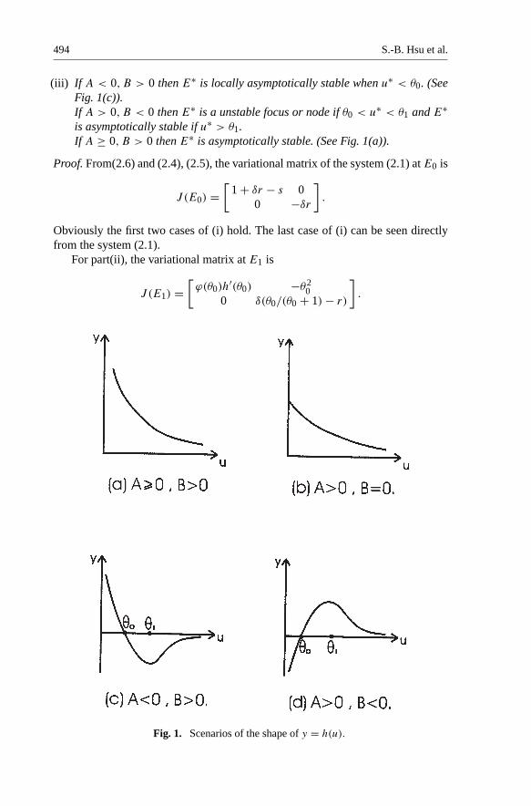
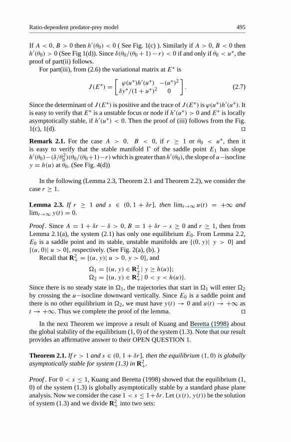
Proof . Since A = 1 + δr − δ > 0, B = 1 + δr − s ≥ 0 and r ≥ 1, then fromLemma 2.1(a), the system (2.1) has only one equilibrium E0. From Lemma 2.2,E0 is a saddle point and its stable, unstable manifolds are {(0, y)| y > 0} and{(u, 0)| u > 0}, respectively. (See Fig. 2(a), (b). )

Recall that R2+ = {(u, y)| u > 0, y > 0}, and

#1 = {(u, y) ∈ R2+| y ≥ h(u)};#2 = {(u, y) ∈ R2+| 0 < y < h(u)}.

Since there is no steady state in #1, the trajectories that start in #1 will enter #2by crossing the u−isocline downward vertically. Since E0 is a saddle point andthere is no other equilibrium in #2, we must have y(t) → 0 and u(t) → +∞ ast → +∞. Thus we complete the proof of the lemma. ��

In the next Theorem we improve a result of Kuang and Beretta (1998) aboutthe global stability of the equilibrium (1, 0) of the system (1.3). Note that our resultprovides an affirmative answer to their OPEN QUESTION 1.

Theorem 2.1. If r > 1 and s ∈ (0, 1 + δr], then the equilibrium (1, 0) is globallyasymptotically stable for system (1.3) in R2+.

Proof . For 0 < s ≤ 1, Kuang and Beretta (1998) showed that the equilibrium (1,0) of the system (1.3) is globally asymptotically stable by a standard phase planeanalysis. Now we consider the case 1 < s ≤ 1+δr . Let (x(t), y(t)) be the solutionof system (1.3) and we divide R2+ into two sets:

496 S.-B. Hsu et al.

Fig. 2. The direction field chart for system (2.1) under various conditions.

Z1 = {(x, y) ∈ R2+| y > h(x), x > 0},Z2 = {(x, y) ∈ R2+| 0 < y ≤ h(x), x ∈ (0, 1)}.

Here y = h(x) = x(1 − x)/((s − 1) + x) is the prey isocline of the system (1.3).Consider the following two cases.

Case 1. x(t) > 1 for all t ≥ 0. Since r ≥ 1 and from (1.3), we have x′(t) < 0and y′(t) < 0 for t > 0. Hence, the limit of (x(t), y(t)) exists as t → +∞. By astandard argument, we conclude that limt→+∞(x(t), y(t)) = (1, 0).

Ratio-dependent predator-prey model 497

Case 2. x(t∗) ≤ 1 for some t∗ ≥ 0. Since the set {(x, y) ∈ R2+|0 < x < 1} ispositive invariant, we have x(t) < 1 for all t > t∗. Claim: There exists T > t∗such that (x(T ), y(T )) ∈ Z2. If the claim does not hold, then (x(t), y(t)) ∈ Z1for all t > t∗. This implies that x′(t) < 0 and y′(t) < 0 for t > t∗ and hencelimt→+∞(x(t), y(t)) = (0, 0). Thus we have(since y > h(x) = x(1 − x)/((s −1) + x))

limt→∞x(t)

y(t)≤ limt→+∞

s − 1 + x(t)

1 − x(t)= s − 1.

On the other hand, x(t)y(t)

= u(t) and from Lemma 2.3 it follows that limt→+∞ u(t) =+∞. This leads to a contradiction and hence we proves the claim.

Since Z2 is positively invariant, we have (x(t), y(t)) ∈ Z2 for t > T . From(1.3), we havex′(t) > 0 andy′(t) < 0 for t > T . Therefore, limt→+∞(x(t), y(t)) =(1, 0). Thus, form both cases, we conclude that the equilibrium (1, 0) is globallystable in R2+. ��

For the case r > 1 and s > 1 + δr , Kuang and Beretta (1998) provedthat the system (1.3) is not persistent by showing the existence of a trajectory(x(t), y(t)) → (0, 0) as t → ∞. In the following we state precisely how the out-comes depend on the initial condition for the system(1.3) or (2.1).

Theorem 2.2. Let r ≥ 1 and s > 1 + δr . For the system (2.1), the stable manifold" of E1 separates R2+ into two regions #1 and #2 such that if (u(0), y(0)) ∈ #1then (u(t), y(t)) → (0, 0) as t → ∞ and if (u(0), y(0)) ∈ #2 then (u(t), y(t)) →(∞, 0) as t → ∞. Equivalently for the system (1.3) there exists a separatrix "′connecting (0, 0) and two regions #′

1, #′2 such that if (x(0), y(0)) ∈ #′

1 then(x(t), y(t)) → (0, 0) as t → ∞ and if (x(0), y(0)) ∈ #′

1 then (x(t), y(t)) →(1, 0) as t → ∞.

Proof . SinceA > 0, B < 0, from Figure 1(d), Remark 2.1 and phase plane analysisthe stable manifold " of E1 lies above the prey isocline y = h(u). Obviously for(u(0), y(0)) ∈ #1, the region on the left of", we have (u(t), y(t)) → (0, 0) as t →∞. For (u(0), y(0)) ∈ #2, the region on the right of ", it follows directly from theproof of Lemma 2.3 that (u(t), y(t)) → (∞, 0) as t → ∞. The statements forthe system (1.3) follows naturally. ��

From now on we discuss the case 0 < r < 1. First we consider the caseδ ≥ 1/(1 − r).

Remark 2.2. It is easy to verify that

(i) δ ≥ 1/(1 − r) if and only if 1/(1 − r) ≤ 1 + δr.

(ii) If B > 0 and A < 0 then u∗ = r/(1 − r) < θ0 = B/(−A) if and only ifs < 1/(1 − r).

(iii) If B < 0 and A > 0 then u∗ < θ0 if and only if 1/(1 − r) < s.

Our next theorem provides YES as the answer to the OPEN QUESTION 2 ofKuang and Beretta (1998).

498 S.-B. Hsu et al.

Theorem 2.3. If r ∈ (0, 1), δ ∈ [1/(1 − r), ∞) and s ∈ (0, 1/(1 − r)) then thepositive equilibrium E∗ exists and is globally asymptotically stable in R2+ for thesystem (2.1).

Proof . From Remark 2.2, r ∈ (0, 1) and s < 1/(1 − r) ≤ δ, we have A =1 + δr − δ ≤ 0 and B = 1 + δr − s ≥ 1/(1 − r) − s > 0. Now we consider thefollowing two cases.

Case 1. A = 0. Lemma 2.1(a) implies that h(u) > 0 > h′(u) for u > 0 . (See Fig.2(c). ) Hence, h(u∗) > 0 > h′(u∗). This shows that the system (2.1) has a uniquepositive equilibrium E∗ and it is locally asymptotically stable.

Case 2. A < 0. Lemma 2.1(b) gives that h(u) and h′(u) has exactly one positivezero θ0, θ1 respectively and θ0 < θ1. (See Fig. 2(e).) Since B > 0, we haveh(u) > 0 > h′(u) for u ∈ (0, θ0). So, h(u∗) > 0 if and only if u∗ < θ0 orequivalently s ∈ (0, 1/(1 − r)) by Remark 2.2 . Hence, the system (2.1) has apositive equilibrium E∗ and from Lemma 2.2 it is locally asymptotically stable.

To show that E∗ is globally asymptotically stable in R2+. Consider the followingLyapunov function

V (u, y) =∫ u

u∗

ψ(ξ)

ϕ(ξ)dξ +

∫ y

y∗

η − y∗

ηdη

for (u, y) ∈ R2+. Notice that (u − u∗)(h(u) − h(u∗)) ≤ 0, which implies thatψ(u)(h(u)− h(u∗)) ≤ 0. The derivative of V along the solution of system (2.1) is

V (u, y) = (g(u) − ϕ(u)y)ψ(u)/ϕ(u) + ψ(u)y − h(u∗)ψ(u)

= ψ(u)(h(u) − h(u∗)) ≤ 0(2.8)

for (u, y) ∈ R2+. Hence, Theorem 2.3 follows from (2.8) and Lyapunov-LaSalle’sinvariance principle (Hale (1980)). ��Theorem 2.4. Let r ∈ (0, 1), δ ∈ [1/(1 − r),∞).

(i) If 1/(1 − r) ≤ s ≤ 1 + δr then the equilibrium E1 = (θ0, 0) of the system(2.1) is globally asymptotically stable.

(ii) If s > 1 + δr then the equilibrium E0 = (0, 0) of the system (2.1) is globallyasymptotically stable.

Proof . From the assumption s > 1/(1 − r) and Remark 2.2 , we have u∗ > θ0. If1/(1−r) ≤ s ≤ 1+δr then A < 0 and B > 0. The prey isocline y = h(u) satisfiesh′(u) < 0 for 0 < u < θ1, h(u) < 0 for u > θ0 and h(u) > 0 for 0 < u < θ0.

From the phase plane analysis it is easy to verify that E1 = (θ0, 0) is globallyasymptotically stable and (i) is proved.

If s > 1+δr then A < 0 and B < 0. Obviously h(u) < 0 for all u > 0, u′(t) <0 for all t > 0 and y′(t) < 0 if and only if u < u∗. From phase plane analysis, theequilibrium E0 = (0, 0) is globally asymptotically stable. ��Remark 2.3. If we return to the original system (1.3), both (i) and (ii) of Theorem 2.4say that the solution (x(t), y(t)) → (0, 0) as t → ∞. The only difference between

Ratio-dependent predator-prey model 499

(i) and (ii) is that x(t)/y(t) → θ0 as t → ∞ in (i) while x(t)/y(t) → 0 as t → ∞in (ii).

Next we consider the case 0 < δ < 1/(1 − r). From Remark 2.2 , we have1 + δr < 1/(1 − r). There are three subcases, namely, 0 < s ≤ 1 + δr, 1 + δr <

s ≤ 1/(1 − r) and s > 1/(1 − r) to be discussed.First we consider the case r ∈ (0, 1), δ ∈ (0, 1/(1 − r)) and s ∈ (0, 1 + δr].

Then we have A = 1 + δr − δ > 0 and B = 1 + δr − s ≥ 0, and Lemma 2.1(a)implies h(u) > 0 > h

′(u) for u > 0. Hence the system (2.1) has a unique positive

equilibrium E∗ and it is locally asymptotically stable. (See Figs.2(c),(d).) Applyingthe same Lyapunov function in the proof of Theorem 2.3, we have the followingtheorem which gives positive answer to the OPEN QUESTION 3 of Kuang andBeretta (1998).

Theorem 2.5. If r ∈ (0, 1), δ ∈ (0, 1/(1 − r)) and s ∈ (0, 1 + δr] then E∗ isglobally asymptotically stable in R2+ for the system (2.1).

Now we consider the case r ∈ (0, 1), δ ∈ (0, 1/(1 − r)) and s ≥ 1/(1 − r).Then A > 0 and B < 0 and from Remark 2.2, we have u∗ < θ0. From Lemma 2.2,E1 = (θ0, 0) is an unstable node and (0, 0) is locally asymptotically stable. Fromthe phase plane analysis, it is easy to show that (0, 0) is globally asymptoticallystable (See Fig. 1(d)). Hence we have:

Theorem 2.6. If r ∈ (0, 1), δ ∈ (0, 1/(1 − r)) and s ≥ 1/(1 − r) the E0 = (0, 0)is globally asymptotically stable in R2+ for the system (2.1).

The last case

r ∈ (0, 1), δ ∈ (0, 1/(1 − r)), 1 + δr < s < 1/(1 − r) (2.9)

is easily the most interesting and important case in this paper.For the rest of this section, we assume that (2.9) holds. Since A = 1+ δr − δ >

0, B = 1 + δr − s < 0, from Remark 2.2 (iii) the system (2.1) has three equilibriaE0 = (0, 0), E1 = (θ0, 0) and E∗ = (u∗, h(u∗)). Moreover from Lemma 2.2,E0 is locally asymptotically stable, E1 is a saddle point and E∗ is unstable(stable)if θ0 < u∗ < θ1(u

∗ > θ1). In the following Theorem 2.7 we assert that the system(2.1) has at most one positive limit cycle.

Theorem 2.7. Let (2.9) hold. Then the system (2.1) has at most one limit cycle inR2+. Moreover, if it exists, then it is a stable limit cycle.

Proof . Let #∗ = (0, θ0] × R+. Then for (u(0), y(0)) ∈ #∗ we have u′(t) < 0 andy′(t) < 0 for t ≥ 0 and hence (u(t), y(t)) → E0 as t → ∞. Thus it suffices toshow that system (2.1) has at most one limit cycle in R2+\#∗. According to Hwang(1999), it suffices to show that

q(u) = ϕ(u)h′(u) − ϕ(u∗)h′(u∗)ψ(u)

(2.10)

500 S.-B. Hsu et al.

is C1 and q ′(u) < 0 for u > 0. From (2.4) and a straight forward computation,it follows that

q(u) = δ − s

δ

((1 + r)u + r)

1 + ufor u > 0. (2.11)

Since δ < 1 + δr < s, we have

q ′(u) = δ − s

δ

1

(1 + u)2< 0 for u > 0. (2.12)

Hence the system (2.1) has at most one limit cycle in R2+ −#∗ and it is stable whenexists. ��

As a result of the above theorem, we see that if E∗ is locally asymptoticallystable, then there is no positive periodic solution surrounding it. This is preciselythe main statement of Theorem 3.1 in Kuang and Beretta (1998).

In the following Lemma 2.4 we classify the behavior of the stable manifold "

of the equilibrium E1.

Lemma 2.4. Let (2.9) hold and " be the stable manifold of E1. Then

(i) If " intersects the prey isocline y = h(u), then " connects E1 and E∗.(ii) If" does not intersects the prey isocline y = h(u) then" = {(u(t), y(t))}+∞

t=−∞satisfies limt→−∞ u(t) = ∞ and limt→−∞ y(t) = 0. Moreover either "′ =γ or "′ lies above γ where "′ = {(x, y) : x = yu, (u, y) ∈ "} and γ is theunstable manifold of the equilibrium (1, 0) for the system (1.3), connecting (1,0) to (0, 0) or (x∗, y∗) in xy−plane.

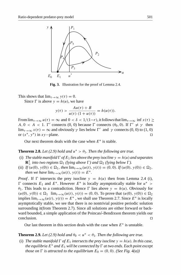
Proof . From Remark 2.1, the stable manifold " of E1 lies above the prey isocliney = h(u) when u > θ0 and u is near θ0. From the phase plane analysis, " is abovethe prey isocline y = h(u) until " meets the predator isocline u = u∗ at t = t∗. If "intersects the prey isocline y = h(u) at point P2, then " will meet u = u∗ at P3, P5and meet y = h(u) at P4 (See Fig. 3). Consider the region # bounded by the arcP1 P2 P3 P4 P5 and segment P5P1. # is negatively invariant. The α-limit set α(P5)

is contained in #. Claim that α(P5) = {E∗}. If not, then α(P5) is a periodic orbit.However from Theorem 2.7, α(P5) is a unique stable limit cycle for the system(2.1). This is a contradiction since α(P5) is unstable from outside. Thus we provethe claim and " connects E1 and E∗.

If " does not intersect the prey isocline y = h(u) then " is above y = h(u).Let τ = −t , then

u′(τ ) = −(u(τ ))2[h(u(τ)) − y(τ)]y′(τ ) = −δy(τ )(u(τ)/(u(τ) + 1) − r).

(2.13)

Then u′(τ ) > 0 and y′(τ ) < 0 for τ > t∗. Obviously limτ→∞ u(τ) = ∞. Hencethere is a t1 > t∗, such that u(t1) = 2u∗. Let

a = 2u∗/(2u∗ + 1) − r.

Then a > 0. For t > t1, we have

y′(τ ) = −δy(τ )(u(τ)/(u(τ) + 1) − r) < −aδy(τ).

Ratio-dependent predator-prey model 501

Fig. 3. Illustration for the proof of Lemma 2.4.

This shows that limτ→∞ y(τ) = 0.Since " is above y = h(u), we have

y(τ) >Au(τ) + B

u(τ) (1 + u(τ))= h(u(τ)).

From limτ→∞ u(τ) = ∞ and 0 < δ < 1/(1−r), it follows that limτ→∞ inf x(τ) ≥A, 0 < A < 1. "′ connects (0, 0) because " connects (θ0, 0). If "′ �= γ thenlimτ→∞ x(τ) = ∞ and obviously γ lies below "′ and γ connects (0, 0) to (1, 0)or (x∗, y∗) in xy−plane. ��

Our next theorem deals with the case when E∗ is stable.

Theorem 2.8. Let (2.9) hold and u∗ > θ1. Then the following are true.

(i) The stable manifold" ofE1 lies above the prey isocline y = h(u) and separatesR2+ into two regions #1 (lying above ") and #2 (lying below ").

(ii) If (u(0), y(0)) ∈ #1, then limt→∞(u(t), y(t)) = (0, 0). If (u(0), y(0)) ∈ #2,

then we have limt→∞(u(t), y(t)) = E∗.Proof . If " intersects the prey isocline y = h(u) then from Lemma 2.4 (i)," connects E1 and E∗. However E∗ is locally asymptotically stable for u∗ >

θ1. This leads to a contradiction. Hence " lies above y = h(u). Obviously for(u(0), y(0)) ∈ #1 limt→∞(u(t), y(t)) = (0, 0). To prove that (u(0), y(0)) ∈ #2implies limt→∞(u(t), y(t)) = E∗ , we shall use Theorem 2.7. Since E∗ is locallyasymptotically stable, we see that there is no nontrivial positive periodic solutionsurrounding it(from Theorem 2.7). Since all solutions are either forward or back-ward bounded, a simple application of the Poincare-Bendixson theorem yields ourconclusion. ��

Our last theorem in this section deals with the case when E∗ is unstable.

Theorem 2.9. Let (2.9) hold and θ0 < u∗ < θ1. Then the following are true.

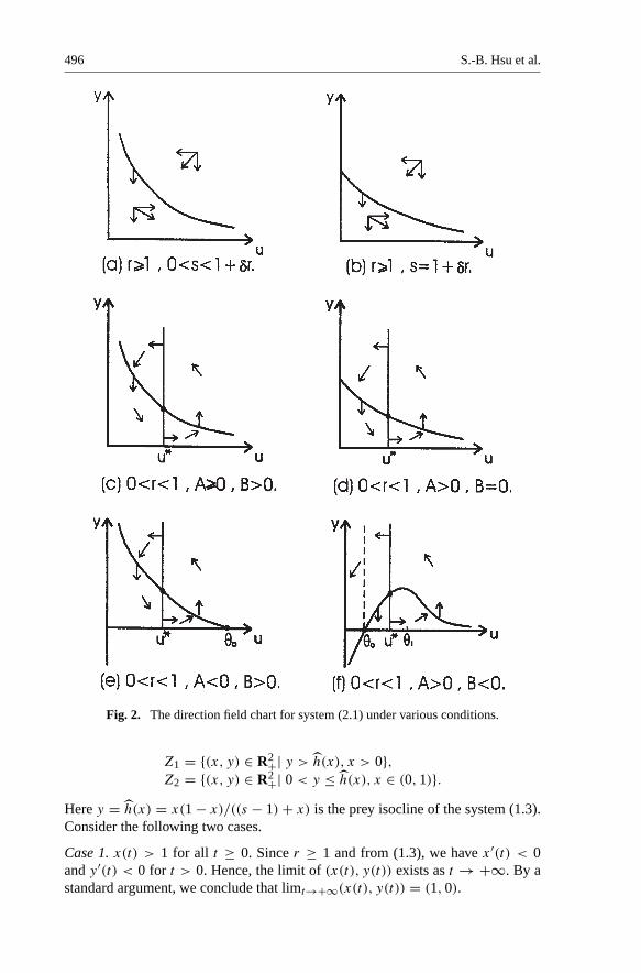
(i) The stable manifold " of E1 intersects the prey isocline y = h(u). In this case,the equilibria E∗ and E1 will be connected by " at two ends. Each point exceptthose on " is attracted to the equilibrium E0 = (0, 0). (See Fig. 4(a))

502 S.-B. Hsu et al.

(ii) The stable manifold " lies above y = h(u) separating R2+ into two regions#1(above") and#2(below"). If (u(0), y(0)) ∈ #1 then limt→∞(u(t), y(t)) =(0, 0). If (u(0), y(0)) ∈ #2 or equivalently (x(0), y(0)) ∈ #′

2(where #′2 =

{(x, y) : x = yu, (u, y) ∈ #2}), then there are two possible cases:(a) The ω-limit set ω(x(0), y(0)) = γ

⋃{(x, y) : y = 0, 0 ≤ x ≤ 1}. (SeeFig. 4(c))

(b) (x(t), y(t)) approaches a unique limit cycle as t → ∞. (See Fig. 4(e))

Proof . If " intersects the prey isocline y = h(u) then from Lemma 2.4 (i), E∗and E1 will be connected by " as two ends. For any (u(0), y(0)) ∈ R2+\", it iseasy to show by phase plane analysis that (u(t), y(t)) ∈ #∗ = (0, θ0] × R+ for tsufficiently large. Thus limt→∞(u(t), y(t)) = E0.

If " does not intersect the prey isocline y = h(u), then " lies above y = h(u).Obviously if (u(0), y(0)) ∈ #1 then limt→∞(u(t), y(t)) = E0. From Lemma2.4 (ii) "′ = γ or "′ lies above γ . Since E∗ = (x∗, y∗) is a unstable fo-cus or node, the unstable manifold γ obviously connects to (0, 0). In this case,we must have "′ = γ. Otherwise, for (x(0), y(0)) in #′

2 lying between "′ andγ, limt→∞(x(t), y(t)) = (0, 0). This indicates that the solutions of system (2.1)with initial data (x(0)/y(0), y(0)) will tend to E1. (can not tend to the origin sinceit is below the stable manifold ".) This implies that the stable manifold " has morethan one trajectories. However, since system (2.1) is continuously differentiable inthe neighborhood of E1, we must have a unique trajectory in ".(Theorem 3.6.1 inHale (1980)) This is a contradiction.

For (x(0), y(0)) lying in the region bounded by γ and {(x, y) : y = 0, 0 ≤x ≤ 1}, there are two possible cases. If the w-limit set ω(x(0), y(0)) containsan equilibrium, then from Butler-McGehee Lemma (Smith and Waltman (1995),p12), ω(x(0), y(0)) = γ

⋃{(x, y) : y = 0, 0 ≤ x ≤ 1}, i.e. (ii)(a) holds. Ifω(x(0), y(0)) contains no equilibrium, then from Poincare-Bendixson Theorem,Theorem 2.7 and that fact that E∗ is unstable, the trajectory (x(t), y(t)) approachesa unique limit cycle. ��

While the case (ii)(a) seems to be unlikely, it can not be ruled out by standardphase plane analysis or from our extensive numerical simulations.

3. Discussion

In this paper we provide a complete classification of the asymptotic behavior of thesolutions of ratio-dependent predator-prey model (1.2). As a result, we solved allthe three open questions listed in Kuang and Beretta (1998) (Theorems 2.1, 2.3,2.5 provide positive answer to OPEN QUESTIONS 1, 2, 3, respectively). The onlyissue left open is how to determine the relative location of the stable manifold� of equilibrium E1 of system (2.1).

Comparing with the classical prey-dependent predator-prey model (1.1), theratio-dependent models (1.2) are capable of producing richer and more reasonabledynamics and the paradox of biological control is no longer valid. In the classicalmodel (1.1), the following results are well known: (Kuang and Freedman (1988))

Ratio-dependent predator-prey model 503

(i) If (K − m)/2 ≤ x∗ then limt→∞(x(t), y(t)) = E∗ = (x∗, y∗) where x∗ =m/((f/d) − 1) > 0, y∗ > 0.

(ii) If (K − m)/2 > x∗ then the solution (x(t), y(t)) approaches a unique limitcycle as t → ∞.

We observe that in the model (1.1), the carrying capacity K plays the key rolein determining the asymptotic behavior of solutions of (1.1). However, for theratio-dependent model (1.2), the asymptotic behavior of the solutions of (1.2) isindependent of the carrying capacity K . On the other hand, the capturing rate c

is independent of the behavior of the solution of model (1.1) while c plays animportant role in the model (1.2). We will elaborate this below.

In the following, we shall discuss the many biological implications of our results(Theorem 2.1–2.9). To facilitate this, recall that s = c/ma, δ = f/a, r = d/f .

First we consider the case r ≥ 1, i.e. the predator death rate d is larger or equalto its maximal growth rate f , then from Theorem 2.1 and Theorem 2.2 the predatorwill go to extinction. Since s > 1 + δr if only if c/m > (a + d). Theorem 2.1 saysif c/m, the ratio of capturing rate c to the half saturation constant m, is small thenthe prey survives and goes to its carrying capacity K . However if c/m is large, forfixed predator initial population y(0), if the ratio x(0)/y(0) is small then both preyand predator go to extinction while if x(0)/y(0) is large then prey survives to itscarrying capacity.

Next, we consider the case 0 < r < 1, i.e. the predator death rate d is less thanits maximal growth rate f . Since δ ≥ 1/(1 − r) if and only if f ≥ d + a and 0 <

s < 1/(1 − r) if and only if 0 < c/m < a/(1 − d/f ), Theorem 2.3 says iff ≥ d +a, i.e., the maximal growth rate f is large or the prey intrinsic growth ratea is small, then the prey and predator coexist in the form of equilibrium providedc/m is small. Under the same conditions of Theorem 2.3, Theorem 2.4 says that ifc/m is large, then both predator and prey go to extinction.

If the prey intrinsic growth rate a > f − d, then predator and prey coexistin the form of equilibrium if c/m is small. Since s > 1/(1 − r) if and only ifc/m > a/(1−(d/f )), Theorem 2.6 states that if a > f −d, then both predator andprey go to extinction provided c/m is large. When a + d < c/m < a/(1 − (d/f )),Theorem 2.7 says that if the ratio at equilibrium (u∗ = x∗/y∗) is large, i.e., u∗ ≥ θ1,and if x(0)/y(0) is small then both predator and prey go to extinction while ifx(0)/y(0) is large then predator and prey coexist in the form of equilibrium.

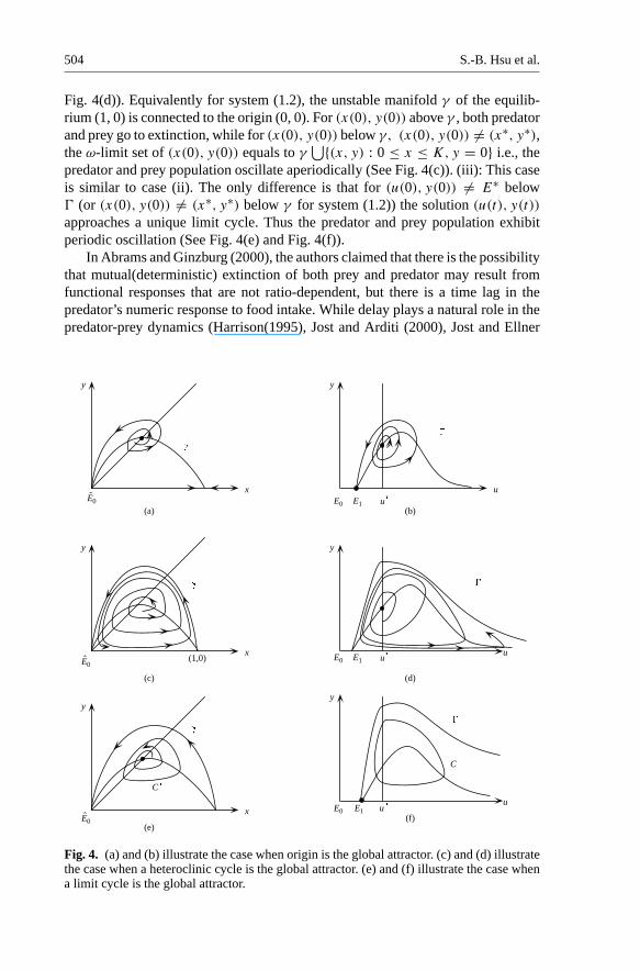
Under the same condition of Theorem 2.7, i.e. a + d < c/m < a/(1 − (d/f )),Theorem 2.8 says if θ0 < u∗ < θ1, there are three possible cases. (i): Thereis an orbit " connecting E1 = (θ1, 0) and E∗ = (u∗, y∗) for the system (2.1)such that for any (u(0), y(0)) /∈ " limt→∞(u(t), y(t)) = (0, 0) (See Fig. 4(b)).Equivalently for system (1.2), there is an orbit "′ connecting (0, 0) and (x∗, y∗)such that for all (x(0), y(0)) /∈ "′, limt→∞(x(t), y(t)) = (0, 0). In this case,except (x(0), y(0)) = (x∗, y∗) both predator and prey go to extinction (See Fig.4(a)). (ii): The stable manifold " of E1 = (θ1, 0) does not intersect the prey iso-cline y = h(u). For (u(0), y(0)) above ", limt→∞(u(t), y(t)) = (0, 0) while for(u(0), y(0)) �= E∗ below ", the ω-limit set of (u(0), y(0)) equals to "

⋃{(u, y):y = 0, u ≥ θ1}, i.e., the solution (u(t), y(t)) exhibit aperiodic oscillation. (See

504 S.-B. Hsu et al.

Fig. 4(d)). Equivalently for system (1.2), the unstable manifold γ of the equilib-rium (1, 0) is connected to the origin (0, 0). For (x(0), y(0)) above γ , both predatorand prey go to extinction, while for (x(0), y(0)) below γ, (x(0), y(0)) �= (x∗, y∗),the ω-limit set of (x(0), y(0)) equals to γ

⋃{(x, y) : 0 ≤ x ≤ K, y = 0} i.e., thepredator and prey population oscillate aperiodically (See Fig. 4(c)). (iii): This caseis similar to case (ii). The only difference is that for (u(0), y(0)) �= E∗ below" (or (x(0), y(0)) �= (x∗, y∗) below γ for system (1.2)) the solution (u(t), y(t))

approaches a unique limit cycle. Thus the predator and prey population exhibitperiodic oscillation (See Fig. 4(e) and Fig. 4(f)).

In Abrams and Ginzburg (2000), the authors claimed that there is the possibilitythat mutual(deterministic) extinction of both prey and predator may result fromfunctional responses that are not ratio-dependent, but there is a time lag in thepredator’s numeric response to food intake. While delay plays a natural role in thepredator-prey dynamics (Harrison(1995), Jost and Arditi (2000), Jost and Ellner

(a)

y

x

y

uE1

(b)

y

x(1,0)

(c)

E0

y

u

(d)

(e)

y

x

C

y

u

C

(f)

E0

E0

E0

E0 E1

E0 E1 u

u

u

Fig. 4. (a) and (b) illustrate the case when origin is the global attractor. (c) and (d) illustratethe case when a heteroclinic cycle is the global attractor. (e) and (f) illustrate the case whena limit cycle is the global attractor.

Ratio-dependent predator-prey model 505

(2000)), we would like to point out that delay alone does not cause mutual extinction.In fact, on the contrary, the delayed numeric response can often moderate the mutualextinction dynamics, due to the fact that in a declining population, the delayednumeric response which in positive correlation to past more robust populationdensity can bring in larger recruitment to the predator population than that can bebrought in by the current smaller population. Near the origin, where both speciesface the possibility of extinction, the predation in the prey-dependent form canbe approximated by a linear form of the product of prey and predator densities,which is no match to the strong recruitment of prey from specific growth. In otherwords, time delay alone will not cause, nor prevent the mutual extinction of bothspecies in both prey-dependent and ratio-dependent cases (as well as for the generalpredator-dependent cases)(Kuang(1993), Beretta and Kuang (1998)).

Deterministic extinction of both species is an extreme outcome of the predator-prey interaction, but seems to become ever more frequent and worrisome. Thepublic believes this resulted from the fragmentation of habitats and the ever shrink-ing sizes of these patches which may diminish or deprive of prey refugees (Fischer(2000)). The consensus view is that ratio dependent formulation breaks down whenthe patch size is large and both the prey and predator densities are low (Arditi andGinzburg (1989), Cosner et al. (1999), Abrams and Ginzburg (2000)), since insuch case, predators will spend most effort in searching rather than interfering eachother. Hence, the functional response is likely to be much more sensible to preydensity than predator density. However, if the habitat is small and free of refugeesfor prey, then ratio dependence formulation may remain valid even when densitiesare low, since predators can remain effectively interfering each other. In such case,ratio-dependence suggests that mutual extinction is possible. This provides an ex-planation for Gause’s classic observation of mutual extinction in the protozoans,Paramecium and its predator Didinium (Abrams and Ginzburg (2000)). In short,deterministic mutual extinction is an extreme outcome calls for extreme measures.Ratio dependence, while a special case of the general predator dependence ones,such as the Beddington-DeAngelis or Hassel-Varley type (Cosner et al. (1999)),is currently the only one that provides a simple and plausible explanation of suchextinction dynamics.

Acknowledgements. The authors would like to thank the referees for their helpful sugges-tions that improved the presentations of both introduction and discussion sections.

References

Abrams, P.A., Ginzburg, L.R.: The nature of predation: prey dependent, ratio-dependent orneither? Trends in Ecology and Evolution, 15, 337–341 (2000)

Akcakaya, H.R., Arditi, R., Ginzburg, L.R.: Ratio-dependent prediction: an abstraction thatworks, Ecology, 76, 995–1004 (1995)

Arditi, R., Berryman, A.A.: The biological paradox, Trends in Ecology and Evolution, 6, 32(1991)

Arditi, R., Ginzburg, L.R.: Coupling in predator-prey dynamics: ratio-dependence, J. Theor.Biol., 139, 311–326 (1989)

506 S.-B. Hsu et al.

Arditi, R., Ginzburg, L.R., Akcakaya, H.R.: Variation in plankton densities among lakes:a case for ratio-dependent models, American Natrualist, 138, 1287–1296 (1991)

Berryman, A.A.: The origins and evolution of predator-prey theory, Ecology, 73, 1530–1535(1992)

Berryman, A.A., Gutierrez, A.P., Arditi, R.: Credible, realistic and useful predator-preymodels, Ecology, 76, 1980–1985 (1995)

Cosner, C., DeAngelis, D.L., Ault, J.S., Olson, D.B.: Effects of spatial grouping on thefunctional response of predators, Theor. Pop. Biol., 56, 65–75 (1999)

Fischer, M.: Species loss after habitat fragmentation, Trends in Ecology and Evolution, 15,396 (2000)

Freedman, H.I.: Deterministic Mathematical Models in Population Ecology, Marcel Dekker,New York (1980)

Gause, G.F.: The struggle for existence, Williams & Wilkins, Baltimore, Maryland, USA(1934)

Hairston, N.G., Smith, F.E., Slobodkin, L.B.: Community structure, population control andcompetition, American Naturalist, 94, 421–425 (1960)

Hale, J.: Ordinary Differential Equations, Krieger Publ. Co., Malabar (1980)Harrison, G.W.: Comparing predator-prey models to Luckinbill’s experiment with Didinium

and Paramecium, Ecology, 76, 357–374 (1995)Hsu, S.-B., Hwang, T.-W.: Global stability for a class of predator-prey systems, SIAM J.

Appl. Math., 55, 763–783 (1995)Hwang, T.-W.: Uniqueness of limit cycle for Gause-type predator-prey systems, J. Math.

Anal. Appl., 238, 179–195 (1999)Jost, C., Arditi, R.: Identifying predator-prey process from time-series, Theor. Pop. Biol.,

57, 325–337 (2000)Jost, C., Ellner, S.P.: Testing for predator dependence in predator-prey dynamics: a non-

parametric approach, Proc. Roy. Soc. Lond. B., 267, 1611–1620 (2000)Jost, C., Arino, O., Arditi, R.: About deterministic extinction in ratio-dependent predator-

prey models, Bull. Math. Biol., 61, 19–32 (1999)Kuang, Y.: Delay Differential Equations with Applications in Population Dynamics. Mathe-

matics in Science and Engineering, 191. Academic Press, Inc., Boston, MA, 1993 (1993)Kuang, Y.: Rich dynamics of Gause-type ratio-dependent predator-prey system, The Fields

Institute Communications, 21, 325–337 (1999)Kuang, Y., Beretta, E.: Global qualitative analysis of a ratio-dependent predator-prey system,

J. Math. Biol., 36, 389–406 (1998)Kuang, Y., Freedman, H.I.: Uniqueness of limit cycles in Gause-type predator-prey ststems,

Math. Biosci., 88, 67–84 (1988)Luck, R.F.: Evaluation of natural enemies for biological control: a behavior approach, Trends

in Ecology and Evolution, 5, 196–199 (1990)May, R.M.: Stability and Complexity in Model Ecosystems, Princeton Univ. Press (1974)Rosenzweig, M.L.: Paradox of enrichment: destabilization of exploitation systems in eco-

logical time, Science, 171, 385–387 (1969)Smith, H., Waltman, P.: The Theory of the Chemostat, Cambridge University Press (1995)