This article appeared in a journal published by Elsevier. The attachedcopy is furnished to the author for internal non-commercial researchand education use, including for instruction at the authors institution

and sharing with colleagues.

Other uses, including reproduction and distribution, or selling orlicensing copies, or posting to personal, institutional or third party

websites are prohibited.

In most cases authors are permitted to post their version of thearticle (e.g. in Word or Tex form) to their personal website orinstitutional repository. Authors requiring further information

regarding Elsevier’s archiving and manuscript policies areencouraged to visit:

http://www.elsevier.com/copyright

Author's personal copy

Effects of a disease affecting a predator on the dynamics ofa predator–prey system

Pierre Auger a, Rachid Mchich b, Tanmay Chowdhury c, Gauthier Sallet d,Maurice Tchuente e, Joydev Chattopadhyay c,�

a UR GEODES, IRD, Centre de Recherche d’lle de France, 32 av. Henri Varagnat, 93143 Bondy cedex, Franceb Ecole Nationale de commerce et de Gestion, B.P. 1255, 90000 Tanger, Moroccoc Agricultural and Ecological Research Unit, Indian Statistical Institute 203, B.T. Road, Kolkata 700108, Indiad UR GEODES, IRD and Project-team MASAIE, INRIA Grand-Est, Francee UR GEODES, IRD and MAT Laboratory, Faculty of Science, University of Yaounde I, P.O. Box 812, Yaounde, Cameroon

a r t i c l e i n f o

Article history:

Received 4 February 2008

Received in revised form

21 October 2008

Accepted 23 October 2008Available online 12 November 2008

Keywords:

Lotka–Volterra model

Predator–prey model

Infected predators

Time scales

Aggregation of variables

Stability

SIRS model

a b s t r a c t

We study the effects of a disease affecting a predator on the dynamics of a predator–prey system. We

couple an SIRS model applied to the predator population, to a Lotka–Volterra model. The SIRS model

describes the spread of the disease in a predator population subdivided into susceptible, infected and

removed individuals. The Lotka–Volterra model describes the predator–prey interactions. We consider

two time scales, a fast one for the disease and a comparatively slow one for predator–prey interactions

and for predator mortality. We use the classical ‘‘aggregation method’’ in order to obtain a reduced

equivalent model. We show that there are two possible asymptotic behaviors: either the predator

population dies out and the prey tends to its carrying capacity, or the predator and prey coexist. In this

latter case, the predator population tends either to a ‘‘disease-free’’ or to a ‘‘disease-endemic’’ state.

Moreover, the total predator density in the disease-endemic state is greater than the predator density in

the ‘‘disease-free’’ equilibrium (DFE).

& 2008 Elsevier Ltd. All rights reserved.

1. Introduction

Ecology and epidemiology are two major and distinct fields ofstudy. However there are situations where some diseases whichare responsible for epidemics, impact heavily on predator–preysystems. For instance, Hethcote et al. (2004) show how thepresence of parasites can change the demographic behavior of apopulation. Such diseases regulate the host population density(Getz and Pickering, 1983) and sometimes help the co-existenceof species (Bairagi et al., 2007). Eco-epidemiology which is arelatively new branch of study in theoretical biology, tackles suchsituations by dealing with both ecological and epidemiologicalissues. It can be viewed as the coupling of an ecologicalpredator–prey (or competition) model and an epidemiologicalSI, SIS or SIRS model. Following Anderson and May (1982) whowere the first to propose an eco-epidemiological model by

merging the ecological predator–prey model introduced by Lotkaand Volterra, and the epidemiological SIR model introduced byKermack and McKendrick, many works have been devoted to thestudy of the effects of a disease on a predator–prey system(Beltrami and Coarrol, 1994; Beretta and Kuang, 1998; Ebert et al.,2000; Freedman, 1990; Hadeler and Freedman, 1989). Mostmodels study predator–prey–parasite systems with microparasi-tic infections (Chattopadhyay and Arino, 1999; Chattopadhyay andBairagi, 2001; Chattopadhyay and Pal, 2002; Freedman, 1990;Hadeler and Freedman, 1989; Venturino, 2002), while a few onesconsider macroparasitic infections (Hudson et al., 1992; Packeret al., 2003). In most microparasitic infection predator–prey models, the parasites infect only the prey population(Chattopadhyay and Arino, 1999; Chattopadhyay and Bairagi,2001; Chattopadhyay and Pal, 2002; Chattopadhyay et al., 2003;Hethcote et al., 2004; Hudson et al., 1992; Xiao and Chen, 2001).In such circumstances, a prey epidemics which would haveevolved towards an endemic state without predators, can die outbecause of the high rate of predation on infectious and hencemore vulnerable prey. Another hypothesis was considered byBairagi et al. (2007), who suggested that the predator may avoidthe infected prey and predate only the susceptible ones, leading toprey extinction. In some other cases, the parasites originally

ARTICLE IN PRESS

Contents lists available at ScienceDirect

journal homepage: www.elsevier.com/locate/yjtbi

Journal of Theoretical Biology

0022-5193/$ - see front matter & 2008 Elsevier Ltd. All rights reserved.

doi:10.1016/j.jtbi.2008.10.030

� Corresponding author. Tel.: +9133 2575 3231; fax: +9133 25773049.

E-mail addresses: pierre.auger@bondy.ird.fr (P. Auger),

racmchich@yahoo.com (R. Mchich),

tanmaychowdhury@yahoo.co.in (T. Chowdhury),

sallet@loria.fr (G. Sallet), Maurice.Tchuente@ens-lyon.fr (M. Tchuente),

joydev@isical.ac.in (J. Chattopadhyay).

Journal of Theoretical Biology 258 (2009) 344–351

Author's personal copy

hosted by the prey, are able to infect the predator and cross thespecies barrier (Hadeler and Freedman, 1989; Venturino, 2002;Anderson and May, 1982). This happens for instance in Hadelerand Freedman (1989) where they consider the possibility of aninfection spreading into the predator population, following thepredation of an infected prey by a susceptible predator.

Among the numerous studies devoted to the effects of adisease on a predator–prey system (Beltrami and Coarrol, 1994;Chattopadhyay et al., 2003; Chattopadhyay and Bairagi, 2001;Chattopadhyay and Arino, 1999; Ebert et al., 2000; Freedman,1990; Hadeler and Freedman, 1989; Hethcote et al., 2004; Hudsonet al., 1992; Mchich et al., 2007; Packer et al., 2003; Xiao and Chen,2001), most contributions consider epidemics affecting the prey,and comparatively less attention has been paid to the effects of adisease affecting the predator (Han et al., 2001; Haque andVenturino, 2007; Hethcote et al., 2004; Venturino, 2002). Thiscontrasts with the empirical evidence that a disease spreading in apopulation of predators can have unexpected effects (Wilmers,2006). The aim of this work is to propose a predator–prey modelin which predators can become infected by a disease. We considertwo time scales, a fast one for the disease and a comparativelyslow one for predator–prey interactions and for predatormortality.

We use the ‘‘aggregation method’’ in order to obtain a reducedequivalent model with variables ðn; pÞ, where n is the prey densityand p is the predator density. We show that this aggregated modelalways has a globally asymptotically stable equilibrium ðn�; p�Þ.Depending on the values of the parameters, this equilibrium iseither predator free, i.e. p� ¼ 0, positive and disease free, i.e.ðn�1; p

�1Þ, with n�140, p�140, p�1 ¼ S�1 þ I�1 þ R�1 and I�1 ¼ 0, or positive

and endemic, i.e. ðn�2; p�2Þ, with n�240, p�240, p�2 ¼ S�2 þ I�2 þ R�2 and

I�240. Moreover, if b is the infection rate and d is the rate at whichinfected predators enter into compartment R, then the inequalityp�1od=bop�2, holds. In other words, the predator density atendemic equilibrium is always greater than the predator densityat disease-free equilibrium (DFE). All these results are obtainedunder the hypothesis that the transmission of the disease followsthe classical mass action law bSI, where S and I are densities suchas population numbers per unit area or unit volume. Morecomplex models of pathogen transmission as functions of thedensities S and I can be considered (McCallum et al., 2001). Forinstance, the asymptotic law of incidence (Anderson and May,1978; Heesterbeek and Metz, 1993; McCallum et al., 2001;Roberts, 1996) has been proposed for populations of phytoplank-ton contaminated by viruses. In Section 5, we analyze a modifiedeco-epidemiological model where the ‘‘true mass action’’ (de Jonget al., 1995) assumed so far is replaced by the asymptotic law ofincidence. For this model, the global asymptotic stability of theequilibrium no longer holds for all values of the parameters.Moreover, contrary to what was observed previously, the predatordensity at endemic equilibrium is always smaller than thepredator density at DFE.

The paper is organized as follows: In the next section themathematical model is presented. The system couples an SIRSmodel to a Lotka–Volterra model. The SIRS model describes thespread of the epidemics in the predator population which isclassically subdivided into susceptible, infected and removedindividuals. This means that we consider diseases in which thelatent period is negligible. We use the Lotka–Volterra model witha prey logistic growth and obtain a structurally stable system. Thismodel is a modification of the classical Lotka–Volterra systemwith density-dependent logistic growth of the prey (Pielou, 1969).Section 3 presents an analysis of the model. We take advantage ofthe two time scales to reduce the dimension of the system byusing the aggregation method (for more details, one can see Augerand Poggiale, 1996; Auger and Roussarie, 1994; Mchich et al.,

2006; Michalski et al., 1997; Auger and Bravo de la Parra, 2000).Section 4 is devoted to the interpretation and the discussion of theresults obtained in Section 3. In Section 5, we analyze a modifiedmodel where the ‘‘true mass action’’ law for disease transmissionis replaced by the asymptotic law of incidence.

2. Assumptions and formulation of the mathematical model

The predator–prey model with a disease affecting the predatorwhich is studied in this paper is the system of four nonlinearordinary differential equations below. In this system, n is the preydensity and S, I, R are, respectively, the susceptible, infected andremoved predator densities. Moreover, it is assumed that thereare two time scales: the slow time scale with t as parameter,corresponds to prey recruitment and predator–prey interactions,whereas the fast time scale with t as parameter, corresponds tothe epidemiological process in the predator population. As aconsequence, t ¼ et, where e51 is a small dimensionless para-meter. In the first equation, the left term is a logistic functioncorresponding to prey recruitment and the right term correspondsto predator–prey interactions. Note that the total predatorpopulation density is p ¼ Sþ I þ R. The last three equationscorrespond to an SIRS model describing the epidemiologicalprocess, coupled with the impact of mortality and predator–preyinteractions on the predator epidemiological compartments. Weuse a classical Kermack–McKendrick with ‘‘true mass action’’(de Jong et al., 1995; McCallum et al., 2001), since S, I and R

represent densities, rather than numbers. This transmission lawhas been used in Beretta and Kuang (1998), Chattopadhyay andPal (2002), Diekmann and Kretzschmar (1991), Hadeler andFreedman (1989), Han et al. (2001), Xiao and Chen (2001) and iscommon to numerous models in the literature.

As assumed above, the disease dynamics is fast whereas themortality and the recruitment of predators are comparativelyslow.

For instance, in the fourth equation, the contribution of theepidemiological process in the time scale t is dR=dt ¼ ðdI � gRÞ

whereas the contribution of predator mortality and recruitmentin the time scale t, is dR=dt ¼ ½�mRþ bnR�, or equivalentlydR=dt ¼ dR=dt � dt=dt ¼ e½�mRþ bnR�, and the fourth equationfollows:

dn

dt¼ � rn 1�

n

K

� �� anðSþ I þ RÞ

h i;

dS

dt ¼ ðgR� bSIÞ þ �½�mSþ bnS�;

dI

dt ¼ ðbSI � dIÞ þ �½�mI � m0I þ bnI�;

dR

dt ¼ ðdI � gRÞ þ �½�mRþ bnR�:

8>>>>>>>>>>><>>>>>>>>>>>:

(1)

The predator–prey parameters of the model are as follows: r isthe prey intrinsic growth rate, K is the prey carrying capacity, a isthe capture rate and b is a parameter related to predatorrecruitment as a consequence of predator–prey interactions. It isusually assumed that b ¼ ea where e is a conversion parameterfrom prey to predator density.

The epidemiological parameters g, b and d represent, respec-tively, the rate at which predators loss immunity, the infectionrate and the rate at which infected predators become immune.

The predator mortality rate is m. We assume that, even if thedisease is a mild one, it has a long term impact on the predatorlongevity. This extra-mortality of infected predators happens atrate m0.

ARTICLE IN PRESS

P. Auger et al. / Journal of Theoretical Biology 258 (2009) 344–351 345

Author's personal copy

Examples of such diseases are infections with asymptomaticcarriers, i.e. diseases where infected individuals have no apparentsymptoms. The behavior of such infected individuals is notmodified, but in the long term their immune system is affectedand becomes less and less efficient. This causes a decrease ofthe average longevity. A first example of such a disease is thetoxoplasmosis for feline species. Feline are the only definitivehosts for this disease which is caused by a single-celled parasitecalled Toxoplasma gondii. Most infected feline do not show anysymptom, but the presence of antibodies to T. gondii in lynx andbobcats suggests that this organism is widespread (Labelle et al.,2001). The predation of hares by lynx is therefore a goodexample illustrating the study carried out in this paper. A secondexample is avian malaria (Cosgrove et al., 2006; Merino et al.,1997) where birds serve as definitive hosts. Indeed, Plasmodiumcan be pathogenic to penguins, domestic poultry, ducks, canaries,falcons and pigeons, but it is most commonly carried asympto-matically by passerine birds which are predators for some insectspecies.

2.1. Aggregated model

We are now going to build an equivalent aggregated systembased on the slow time scale, by assuming that the completesystem is permanently in a state corresponding to the fastequilibrium.

2.1.1. Case 1: R0o1When R0o1, which is equivalent to pod=b, the unique

nonnegative fast equilibrium is ðp;0;0Þ, hence I ¼ 0. The aggre-gated system is

dn

dt¼ n r 1�

n

K

� �� ap

h i;

dp

dt¼ pð�mþ bnÞ:

8>><>>: (2)

2.1.2. Case 2: R041When R041, which is equivalent to p4d=b, the unique fast

equilibrium is the one exhibited in Section 3.1. This equilibrium isendemic and the corresponding aggregated system is

dn

dt¼ n r 1�

n

K

� �� ap

h i;

dp

dt¼ �mp�

m0ggþ d

p�db

� �þ bnp:

8>>><>>>:

(3)

This shows that, depending on p, the aggregated model is eithersystem (2) or system (3). Let us now subdivide the positivequadrant ðn; pÞ into two sub-domains:

D1 ¼ ½0;þ1Þ � 0;db

� �and D2 ¼ ½0;þ1Þ �

db;þ1

� �.

In sub-domain D1 the aggregated system (2) is valid, whereas insubdomain D2 system (3) holds. This latter system looks like aLotka–Volterra system, but with a constant immigration in thepredator population.

2.1.3. Dynamics of the aggregated system

Let X1ðn; pÞ be the vector field associated with (2) on R2, and letX2ðn; pÞ be the vector field associated with (3) on R2. Theaggregated system is defined on the nonnegative orthant R2

þ bya vector field which is equal to X1 on the closure of D1 and is equalto X2 on D2. To summarize, let us denote Xðn; pÞ the aggregated

vector field defined by the following equation:

Xðn; pÞ ¼ X1ðn; pÞ ¼n½rð1� n

KÞ � ap�

pð�mþ bnÞ

" #if ðn; pÞ 2 closure ðD1Þ;

Xðn; pÞ ¼ X2ðn; pÞ

¼

n½rð1� nKÞ � ap�

�mp� m0ggþd ðp�

dbÞ þ bnp

24

35 if ðn; pÞ 2 D2:

8>>>>>>>><>>>>>>>>:

(4)

It is straightforward to check that this vector field is continuouson the entire positive orthant, and is C1 on the subsets D1 and D2.Moreover, starting from any point of the boundary between D1

and D2, i.e. if initially R0 ¼ 1 or equivalently p ¼ d=b, thetrajectory issued from this vector field leaves instantaneouslythe boundary.

It follows from classical results on dynamical systems, that thisvector field has a unique solution for any initial condition in theorthant.

2.2. Equilibria and stability

We are now going to compute the ‘‘slow’’ equilibria of thedynamical system associated with X on the positive orthant. Thenwe will analyze their stability.

On R2 the vector field X1 has there equilibria: ð0;0Þ, ðK;0Þ andðn�1; p

�1Þ where n�1 ¼ m=b and p�1 ¼ r=að1� m=bKÞ.

On R2 the vector field X2 has two equilibria: ð0; pÞ 2 D1 with

p ¼1

1þmðgþ dÞm0g

dbo

db

and ðn�2; p�2Þ with

p�2 ¼r

a

�b½ðdþ gÞ ðm� bKÞ þ m0g� þffiffiffiffiDp

2b bKðdþ gÞ

!40

and

n�2 ¼ K 1�a

rp�2

� �,

where

D ¼ b2½ðdþ gÞðm� bKÞ þ m0g�2 þ 4abKbm0dgðdþ gÞ

r40.

For each equilibrium ðn�i ; p�i Þ, i ¼ 1;2; we have a corresponding

basic reproduction number

Ri;�0 ¼

bd

p�i .

Theorem 2.1. With the preceding notations, the following properties

hold:

� The trivial equilibrium ð0;0Þ is a saddle point.� If p�1o0, then the PFE ðK;0Þ is GAS.� If 0op�1od=b or equivalently R1;�

0 o1, then the equilibrium state

ðn�1; p�1Þ 2 D1 is GAS on the positive orthant.

� If d=bop�1 or equivalently R1;�0 41, then the equilibrium state

ðn�2; p�2Þ 2 D2 is GAS on the positive orthant.

Proof. See Appendix A.

2.3. Numerical results

In this section we present some simulations which illustrateTheorem 2.1. Hereafter, blue lines are trajectories of the system,

ARTICLE IN PRESS

P. Auger et al. / Journal of Theoretical Biology 258 (2009) 344–351346

Author's personal copy

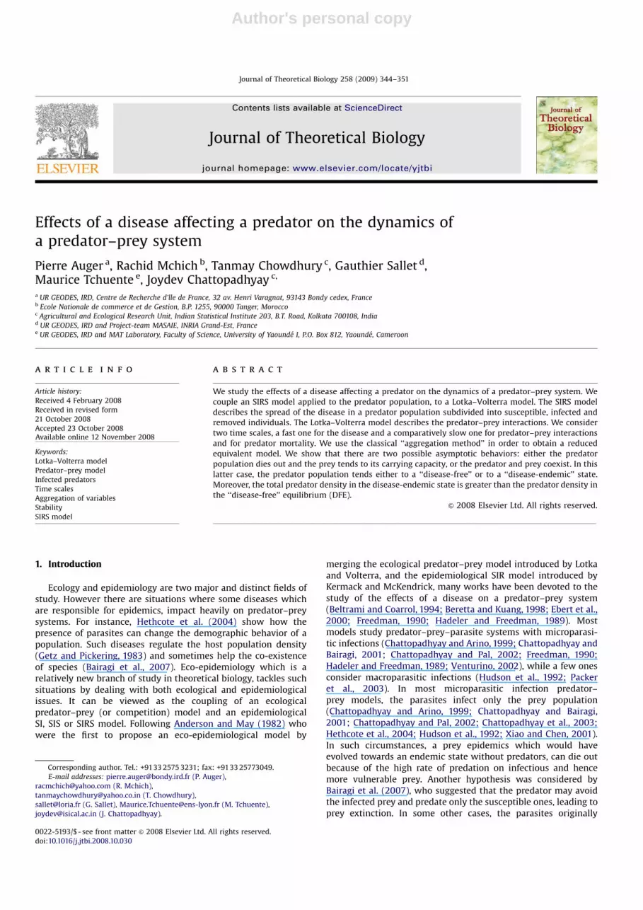
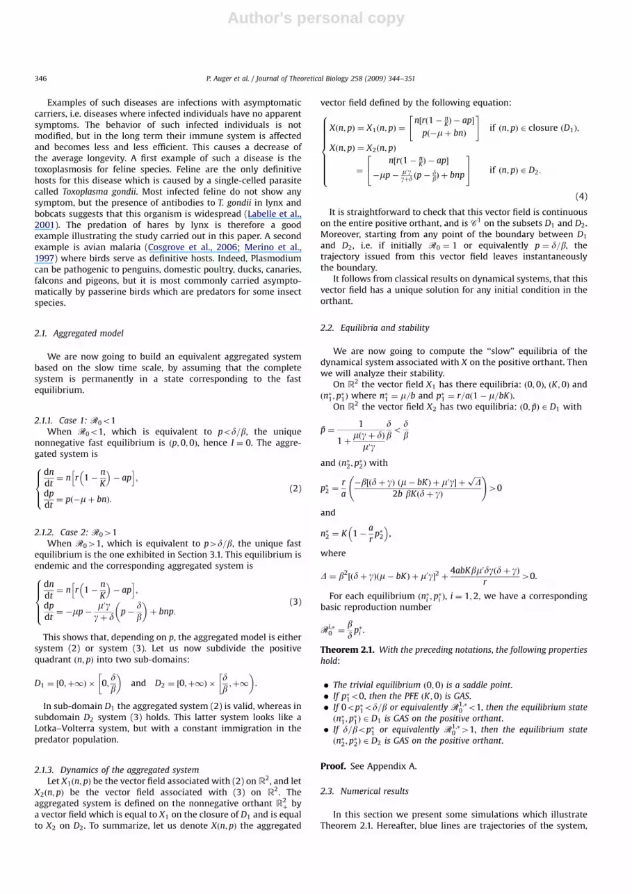
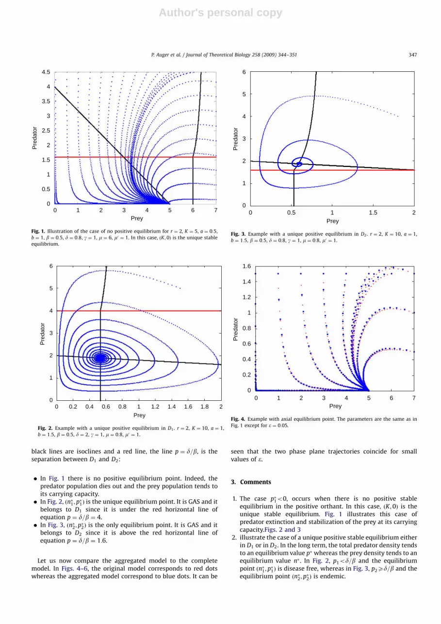
black lines are isoclines and a red line, the line p ¼ d=b, is theseparation between D1 and D2:

� In Fig. 1 there is no positive equilibrium point. Indeed, thepredator population dies out and the prey population tends toits carrying capacity.� In Fig. 2, ðn�1; p

�1Þ is the unique equilibrium point. It is GAS and it

belongs to D1 since it is under the red horizontal line ofequation p ¼ d=b ¼ 4.� In Fig. 3, ðn�2;p

�2Þ is the only equilibrium point. It is GAS and it

belongs to D2 since it is above the red horizontal line ofequation p ¼ d=b ¼ 1:6.

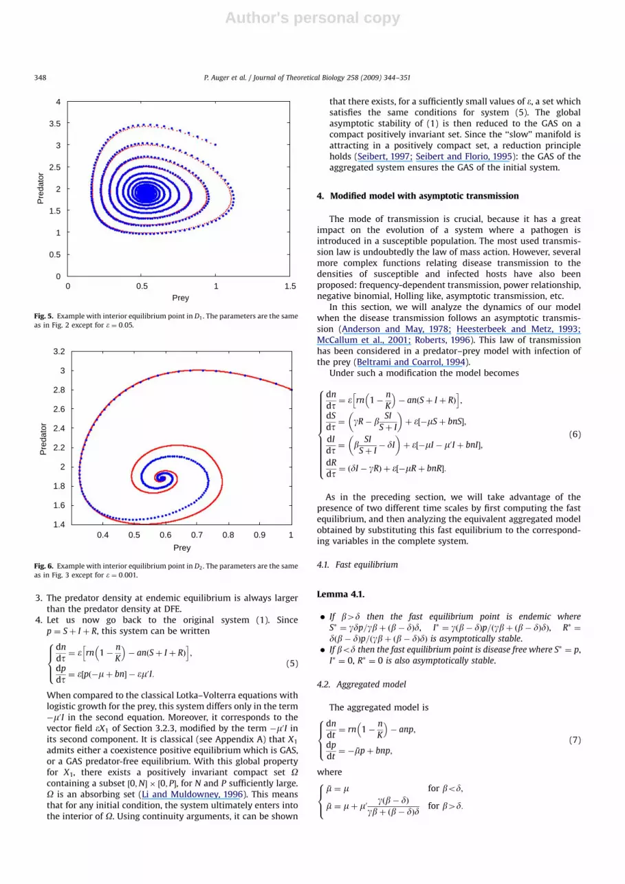
Let us now compare the aggregated model to the completemodel. In Figs. 4–6, the original model corresponds to red dotswhereas the aggregated model correspond to blue dots. It can be

seen that the two phase plane trajectories coincide for smallvalues of �.

3. Comments

1. The case p�1o0, occurs when there is no positive stableequilibrium in the positive orthant. In this case, ðK;0Þ is theunique stable equilibrium. Fig. 1 illustrates this case ofpredator extinction and stabilization of the prey at its carryingcapacity.Figs. 2 and 3

2. illustrate the case of a unique positive stable equilibrium eitherin D1 or in D2. In the long term, the total predator density tendsto an equilibrium value p� whereas the prey density tends to anequilibrium value n�. In Fig. 2, p1od=b and the equilibriumpoint ðn�1; p

�1Þ is disease free, whereas in Fig. 3, p2Xd=b and the

equilibrium point ðn�2; p�2Þ is endemic.

ARTICLE IN PRESS

4.5

4

3.5

3

2.5

2

1.5

1

0.5

00 1 2 3 4 5 6 7

Prey

Pre

dato

r

Fig. 1. Illustration of the case of no positive equilibrium for r ¼ 2, K ¼ 5, a ¼ 0:5,

b ¼ 1, b ¼ 0:5, d ¼ 0:8, g ¼ 1, m ¼ 6, m0 ¼ 1. In this case, ðK;0Þ is the unique stable

equilibrium.

6

5

4

3

2

1

00 0.2 0.4 0.6 0.8 1.21 1.4 1.6 1.8 2

Prey

Pre

dato

r

Fig. 2. Example with a unique positive equilibrium in D1. r ¼ 2, K ¼ 10, a ¼ 1,

b ¼ 1:5, b ¼ 0:5, d ¼ 2, g ¼ 1, m ¼ 0:8, m0 ¼ 1.

6

5

4

3

2

1

0

Pre

dato

r

0 0.5 1 1.5 2Prey

Fig. 3. Example with a unique positive equilibrium in D2. r ¼ 2, K ¼ 10, a ¼ 1,

b ¼ 1:5, b ¼ 0:5, d ¼ 0:8, g ¼ 1, m ¼ 0:8, m0 ¼ 1.

1.6

1.4

1.2

1

0.8

0.6

0.4

0.2

0

Pre

dato

r

0 1 2 3 4 5 6 7Prey

Fig. 4. Example with axial equilibrium point. The parameters are the same as in

Fig. 1 except for � ¼ 0:05.

P. Auger et al. / Journal of Theoretical Biology 258 (2009) 344–351 347

Author's personal copy

3. The predator density at endemic equilibrium is always largerthan the predator density at DFE.

4. Let us now go back to the original system (1). Sincep ¼ Sþ I þ R, this system can be written

dn

dt ¼ � rn 1�n

K

� �� anðSþ I þ RÞ

h i;

dp

dt ¼ �½pð�mþ bn� � �m0I:

8>><>>: (5)

When compared to the classical Lotka–Volterra equations withlogistic growth for the prey, this system differs only in the term�m0I in the second equation. Moreover, it corresponds to thevector field �X1 of Section 3.2.3, modified by the term �m0I inits second component. It is classical (see Appendix A) that X1

admits either a coexistence positive equilibrium which is GAS,or a GAS predator-free equilibrium. With this global propertyfor X1, there exists a positively invariant compact set Ocontaining a subset ½0;N� � ½0; P�, for N and P sufficiently large.O is an absorbing set (Li and Muldowney, 1996). This meansthat for any initial condition, the system ultimately enters intothe interior of O. Using continuity arguments, it can be shown

that there exists, for a sufficiently small values of �, a set whichsatisfies the same conditions for system (5). The globalasymptotic stability of (1) is then reduced to the GAS on acompact positively invariant set. Since the ‘‘slow’’ manifold isattracting in a positively compact set, a reduction principleholds (Seibert, 1997; Seibert and Florio, 1995): the GAS of theaggregated system ensures the GAS of the initial system.

4. Modified model with asymptotic transmission

The mode of transmission is crucial, because it has a greatimpact on the evolution of a system where a pathogen isintroduced in a susceptible population. The most used transmis-sion law is undoubtedly the law of mass action. However, severalmore complex functions relating disease transmission to thedensities of susceptible and infected hosts have also beenproposed: frequency-dependent transmission, power relationship,negative binomial, Holling like, asymptotic transmission, etc.

In this section, we will analyze the dynamics of our modelwhen the disease transmission follows an asymptotic transmis-sion (Anderson and May, 1978; Heesterbeek and Metz, 1993;McCallum et al., 2001; Roberts, 1996). This law of transmissionhas been considered in a predator–prey model with infection ofthe prey (Beltrami and Coarrol, 1994).

Under such a modification the model becomes

dn

dt¼ � rn 1�

n

K

� �� anðSþ I þ RÞ

h i;

dS

dt¼ gR� b

SI

Sþ I

� �þ �½�mSþ bnS�;

dI

dt¼ b

SI

Sþ I� dI

� �þ �½�mI � m0I þ bnI�;

dR

dt ¼ ðdI � gRÞ þ �½�mRþ bnR�:

8>>>>>>>>>>>><>>>>>>>>>>>>:

(6)

As in the preceding section, we will take advantage of thepresence of two different time scales by first computing the fastequilibrium, and then analyzing the equivalent aggregated modelobtained by substituting this fast equilibrium to the correspond-ing variables in the complete system.

4.1. Fast equilibrium

Lemma 4.1.

� If b4d then the fast equilibrium point is endemic where

S� ¼ gdp=gbþ ðb� dÞd, I� ¼ gðb� dÞp=ðgbþ ðb� dÞdÞ, R� ¼

dðb� dÞp=ðgbþ ðb� dÞdÞ is asymptotically stable.� If bod then the fast equilibrium point is disease free where S� ¼ p,

I� ¼ 0, R� ¼ 0 is also asymptotically stable.

4.2. Aggregated model

The aggregated model is

dn

dt¼ rn 1�

n

K

� �� anp;

dp

dt¼ �mpþ bnp;

8>><>>: (7)

where

m ¼ m for bod;

m ¼ mþ m0 gðb� dÞgbþ ðb� dÞd

for b4d:

8><>:

ARTICLE IN PRESS

4

3.5

3

2.5

2

1.5

1

0.5

0

Pre

dato

r

0 0.5 1 1.5Prey

Fig. 5. Example with interior equilibrium point in D1. The parameters are the same

as in Fig. 2 except for � ¼ 0:05.

3.2

3

2.8

2.6

2.4

2.2

2

1.8

1.6

1.4

Pre

dato

r

Prey0.4 0.5 0.6 0.7 0.8 0.9 1

Fig. 6. Example with interior equilibrium point in D2. The parameters are the same

as in Fig. 3 except for � ¼ 0:001.

P. Auger et al. / Journal of Theoretical Biology 258 (2009) 344–351348

Author's personal copy

4.3. Equilibrium points and stability analysis of the aggregated

model There are three possible equilibrium points for theaggregated model (7):

� (0,0) which is a always saddle point.� ðK;0Þ which is a stable equilibrium if Kom=b and saddle point

otherwise.� ðn�; p�Þ where n� ¼ m=b and p� ¼ r=að1� m=bKÞ. This last

equilibrium is stable if K4m=b and is a saddle point otherwise.The interior equilibrium point shows that the predator densityin the DFE is larger than the predator density in the endemicequilibrium.

In this model, the comparison of the predator densities ofdisease free and endemic equilibria, lead to a conclusion oppositeto what we found in the model with the law of mass action.

5. Conclusion

In this paper, we have studied the effects of a disease affectinga predator, on the dynamics of a predator–prey system. The SIRSmodel with simple mass action law was first used to describe thespread of the disease in the predator population. In this model, thepopulation is divided into three compartments, namely suscep-tible, infected and removed individuals. On the other hand, thepredator–prey interactions were modeled by the classical Lotka–Volterra equations.

It was assumed that there are two time scales, a fast one for thedisease and a comparatively slow one for predator–prey interactionsand for predator mortality. The ‘‘aggregation method’’ was used inorder to obtain a reduced equivalent system with parameters ðn; pÞ,where n is the fast equilibrium value for the prey population and n isthe fast equilibrium value for the predator population. Since thereare two possible fast equilibria which are stable, the aggregatedmodel uses a vector field X1 if pod=b, and another vector field X2

otherwise. The analysis carried out here shows that the aggregatedsystem has three possible equilibria which are GAS: a predator-freeequilibrium ðK;0Þ, a positive disease-free equilibrium ðn�1; p

�1Þ, with

p�1od=b, and a positive endemic equilibrium ðn�2; p�2Þ, with p�2Xd=b.

The fact that the predator population p2 at endemic equilibrium isgreater than the predator population p1 at disease-free equilibrium isconsistent with the fact, in SIRS models with standard mass actionlaw, the basic reproduction number R0 is an increasing function ofthe total density. Then we have studied the dynamics of the systemwhen the disease transmission follows an asymptotic incidence law.In this case, the predator population at DFE is greater than thepredator population at endemic equilibrium.

We have therefore considered two transmission laws whichlead to opposite conclusions with respect to the predator densitiesat equilibrium. In practice, the choice of the adequate transmis-sion law is crucial but somewhat difficult. For example de Jong etal. (1995) analyzed data from the Pasterella muris laboratoryepidemics in mice modeled by Anderson and May (1978), andconcluded that frequency-dependent (i.e. SI=N) and density-dependent transmission (i.e. mass action) models fitted the dataequally well. The same authors remark that the ‘‘true mass-action’’ assumption is valid whenever individuals move randomlywithin the space in which population lives, with ‘‘contacts’’corresponding to ‘‘collisions’’.

All the results presented here are based on the classic SIRSepidemic. Moreover predator–prey interactions are modeled by aLotka–Volterra system whose parameters are independent of thepredator epidemiological status. It may be interesting to see whathappens with more complex epidemic models, different transmis-sion laws and other predator response functions such as Hollingtypes II and III.

Appendix A

In this appendix we give the proof of Theorem 2.1.We use the notation of Section 2.2. To prove the theorem we

begin to prove two results on the equilibria of the vector field X1

and X2.

Lemma 6.1. The assertion ðn�2; p�2Þ 2 D2 is equivalent to ðn�1; p

�1Þ 2 D2.

ðn�2; p�2Þ 2 D1 is equivalent to ðn�1; p

�1Þ 2 D1.

Proof. We recall p�1 ¼ ðr=aÞð1� m=bKÞ and

p�2 ¼rb½ðdþ gÞðbK � mÞ � m0g� þ

ffiffiffiffiffiffiffiffiffiffiffiffiffiffiffiffiffiffiffiffiffiffiffiffiffiffiffiffiffiffiffiffiffiffiffiffiffiffiffiffiffiffiffiffiffiffiffiffiffiffiffiffiffiffiffiffiffiffiffiffiffiffiffiffiffiffiffiffiffiffiffiffiffiffiffiffiffiffiffiffiffiffiffiffiffiffiffiffiffiffiffiffiffiffiffiffiffiffiffiffiffiffiffiffiffiffir2b2½ðdþ gÞðbK � mÞ � m0g�2 þ 4abKbm0dgrðdþ gÞ

q2abbKðdþ gÞ .

We can rewrite this expression as

p�2 ¼p�12� cþ

ffiffiffiffiffiffiffiffiffiffiffiffiffiffiffiffiffiffiffiffiffiffiffiffiffiffiffiffiffiffiffiffiffiffiffiffiffiffiffiffip�12� c

� �2

þ 2dcb

s,

where

c ¼rm0g

2abKðgþ dÞ.

Suppose now that ðp�2Þ 2 D2, which is equivalent to p�24d=b orequivalentlyffiffiffiffiffiffiffiffiffiffiffiffiffiffiffiffiffiffiffiffiffiffiffiffiffiffiffiffiffiffiffiffiffiffiffiffiffiffiffiffi

p�12�c

� �2

þ 2dcb

s4

db�

p�12þc

� �.

We distinguish two cases:

The first one is d=b� p�1=2þ co0, which implies p�140 and

d=bop�1=2op�1. In other words ðn�1; p�1Þ 2 D2.

The second one is d=b� p�1=2þc40 which implies

ffiffiffiffiffiffiffiffiffiffiffiffiffiffiffiffiffiffiffiffiffiffiffiffiffiffiffiffiffiffiffiffiffiffiffiffiffiffiffiffip�12� c

� �2

þ 2dcb

s0@

1A

2

4db�

p�12þc

� �2

,

which gives ðd=bÞðd=b� p�1=2Þo0, hence ðn�1;p�1Þ 2 D2.

The second equivalence is obtained by an identical proof: By

continuity we obtain nonstrict inequalities, the equivalence of

negations gives the results. This ends the proof of the lemma. &

Lemma 6.2. The equilibrium ðn�2; p�2Þ is globally asymptotically stable

on the positive orthant for X2.

If p�140 then ðn�1; p�1Þ is globally asymptotically stable on the

positive orthant.

Proof. The proof use classical Lyapunov functions for Lotka–Volterra systems (Goh, 1976; Harrison, 1979). For the two systemswe consider, on the positive orthant

Viðn; pÞ ¼b

aðn� n�i lnðnÞ � n�i þ n�i lnðn�i ÞÞ

þ ðp� p�i lnðpÞ � p�i þ p�i lnðp�i ÞÞ.

Writing X1 as

X1ðn; pÞ ¼an½ r

aK ðn�1 � nÞ þ ðp�1 � pÞ�

bpðn� n�1Þ

" #.

For X2 we set a ¼ m0gd=ðgþ dÞb so that we can write X2 as

X2ðn; pÞ ¼an½ r

aK ðn�2 � nÞ þ ðp�2 � pÞ�

p½bðn� n�2Þ þ ap�

2�p

pp�2�

24

35.

ARTICLE IN PRESS

P. Auger et al. / Journal of Theoretical Biology 258 (2009) 344–351 349

Author's personal copy

It is now straightforward to obtain the derivatives of Vi alongthe trajectories of Xi

_V1 ¼ �b

aKðn� n�1Þ

2p0

and

_V2 ¼ �b

aKðn� n�2Þ

2� aðp�2 � pÞ2

pp�2p0.

Using Lyapunov theorems for X1 and X2, with LaSalle’sinvariance principle for X1 we conclude to of the equilibria.

The Jacobian matrix J0 of X1 computed at (0,0) is given by

J0 ¼r 0

0 �m

" #.

For any value of the parameters the origin is a saddle point. Its

stable manifold is the p-axis.

The Jacobian matrix J1 of X1 computed at ðn�1; p�1Þ is given by

J1 ¼�

rn�1

K �an�1bp�1 0

" #.

The Jacobian matrix JK of X1 computed at ðK ;0Þ is

JK ¼�r �aK

0 �mþ bK

" #.

The Jacobian matrix J2 of X2 computed at ðn�2; p�2Þ is given by

J2 ¼�

rn�2

K �an�2

bp�2 �m0ggþd

db

1p�

2

24

35.

If p�1o0, from Lemma 6.1, this implies ðn�2; p�2ÞeD2. The Jacobian

matrix JK shows that ðK ;0Þ is the unique asymptotic stable

equilibrium of the aggregated vector field X.

If 0op�1od=b. Then ðn�1; p�1Þ 2 D1 and ðn�2; p

�2Þ 2 D1 by Lemma 6.1.

With Lemma 6.2 we deduce that ðn�1; p�1Þ 2 D1 is asymptotically

stable for X (at least locally) and that any trajectory of X starting in

D2 enters D1.

If p�14d=b then ðn�1; p�1Þ 2 D2 and ðn�2; p

�2Þ 2 D2 by Lemma 6.1.

With Lemma 6.2 we deduce that ðn�2; p�2Þ 2 D2 is asymptotically

stable for X (at least locally) and that any trajectory of X starting in

D1 enters D2.

To prove the global stability, it is now sufficient to eliminate the

possibility of limit cycles. A theoretical possibility is a trajectory

starting from the boundary of D1, entering D2 (e.g. in case 3),

and cycling with the first trajectory. With the properties of X we

can use Dulac criterion with Bðn; pÞ ¼ 1=np. A closed path cannot

exist if

qqnðBPiÞ þ

qqpðBQiÞ

has the same sign, where Pi and Qi are, respectively, the first and

second components of the vector field Xi.

We have

qqnðBP1Þ þ

qqpðBQ1Þ ¼ �

r

K

and

qqnðBP2Þ þ

qqpðBQ2Þ ¼ �

r

K�

m0gdðdþ gÞb

1

np2.

This ends the proof of the theorem. &

References

Anderson, R.M., May, R., 1978. Regulation and stability of host-parasite interac-tions. I. Regulatory processes. J. Anim. Ecol. 47, 219–247.

Anderson, R.M., May, R., 1982. The invasion, persistence and spread of infectiousdiseases within animal and plant communities. Philos. Trans. R. Soc. Lond. BBiol. Sci. 314, 533–570.

Auger, P., Bravo de la Parra, R., 2000. Methods of aggregation of variables inpopulation dynamics. C. R. Acad. Sci. III 323, 665–674.

Auger, P., Poggiale, J.-C., 1996. Emergence of population growth model: fastmigration and slow growth. J. Theor. Biol. 182, 99–108.

Auger, P., Roussarie, R., 1994. Complex ecological models with simple dynamics:from individuals to population. Acta Biol. 42, 111–136.

Bairagi, N., Roy, P., Chattopadhyay, J., 2007. Role of infection on the stability of apredator–prey system with several response functions. A comparative study.J. Theor. Biol. 248, 10–25.

Beltrami, E., Coarrol, T., 1994. Modelling the role of viral disease in recurrentphytoplankton blooms. J. Math. Biol. 32, 857–863.

Beretta, E., Kuang, Y., 1998. Modeling and analysis of a marine bacteriophageinfection. Math. Biosci. 149, 57–76.

Chattopadhyay, J., Arino, O., 1999. A predator–prey model with disease in the prey.Nonlinear Anal. 36, 747–766.

Chattopadhyay, J., Bairagi, N., 2001. Pelicans at risk in salton sea—an ecoepide-miological study. Ecol. Model. 136.

Chattopadhyay, J., Pal, S., 2002. Viral infection on phytoplankton zooplanktonsystem—a mathematical model. Ecol. Model. 151, 15–28.

Chattopadhyay, J., Srinivasu, P., Bairagi, N., 2003. Pelicans at risk in salton sea—anecoepidemiological model-ii. Ecol. Model. 167, 199–211.

Cosgrove, C.L., Knowles, S.C.L., Day, K.P., Sheldon, B.C., 2006. No evidence for avianmalaria infection during the nestling phase in a passerine bird. J. Parasitol. 92,1302–1304.

de Jong, M., Diekmann, O., Heesterbeek, H., 1995. How does transmission ofinfection depend on population size? In: Mollison, D. (Ed.), Epidemic Models.Their Structure and Relation to Data. Cambridge University Press, Cambridge,pp. 85–94, 539–570.

Diekmann, O., Kretzschmar, M., 1991. Patterns in the effects of infectious diseaseson population growth. J. Math. Biol. 29, 539–570.

Ebert, D., Lipsitch, M., Mangin, K., 2000. The effect of parasites on host populationdensity and extinction: experimental epidemiology with daphnia and sixmicroparasites. Am. Nat. 156.

Freedman, H.I., 1990. A model of predator–prey dynamics as modified by the actionof a parasite. Math. Biosci. 99, 143–155.

Getz, W.M., Pickering, J., 1983. Epidemic models: thresholds and populationregulation. Am. Nat. 121, 892–898.

Goh, B.S., 1976. Global stability in two species interactions. J. Math. Biol.313–318.

Hadeler, K.P., Freedman, H.I., 1989. Predator–prey populations with parasiticinfection. J. Math. Biol. 27, 609–631.

Han, L., Ma, Z., Hethcote, H.W., 2001. Four predator prey models with infectiousdiseases. Math. Comput. Modelling 34, 849–858.

Haque, M., Venturino, E., 2007. An ecoepidemiological model with disease inpredator: the ratio-dependent case. Math. Methods Appl. Sci. 30,1791–1809.

Harrison, G.W., 1979. Global stability of predator–prey interactions. J. Math. Biol. 8,159–171.

Heesterbeek, J.A., Metz, J.A., 1993. The saturating contact rate in marriage andepidemic models. J. Math. Biol. 31, 529–539.

Hethcote, H.W., Wang, W., Han, L., Ma, Z., 2004. A predator–prey model withinfected prey. Theor. Popul. Biol. 66, 259–268.

Hudson, P., Dobson, A., Newborn, D., 1992. Do parasites make prey vulnerable topredation? Red grouse and parasites. Anim. Ecol. 61, 681–692.

Labelle, P., Dubey, J., Mikaelian, I., Blanchette, N., Lafond, R., St-Onge, S., Martineau,D., 2001. Seroprevalence of antibodies to Toxoplasma gondii in lynx (Lynxcanadensis) and bobcats (Lynx rufus) from Quebec, Canada. J. Parasitol. 87,1194–1196.

Li, M.Y., Muldowney, J.S., 1996. A geometric approach to global-stability problems.SIAM J. Math. Anal. 27, 1070–1083.

McCallum, H., Barlow, N., Hone, J., 2001. How should pathogen transmission bemodelled? Trends Ecol. Evol. 16, 295–300.

Mchich, R., Auger, P., Lett, C., 2006. Effects of aggregative and solitary individualbehaviors on the dynamics of predator–prey game models. Ecol. Model. 197,281–289.

Mchich, R., Auger, P., Poggiale, J.-C., 2007. Effect of predator density dependentdispersal of prey on stability of a predator–prey system. Math. Biosci. 206,343–356.

Merino, S., Potti, J., Fargallo, J.A., 1997. Blood parasites of passerine birds fromcentral spain. J. Wildl. Dis. 33, 638–641.

Michalski, J., Poggiale, J.-C., Arditi, R., Auger, P., 1997. Macroscopic dynamicseffects of migrations in patchy predator–prey system. J. Theor. Biol. 185,459–474.

Packer, C., Holt, R., Hudson, P., Lafferty, K., Dobson, A., 2003. Keeping the herdshealthy and alert: implications of predator control for infectious disease. Ecol.Lett. 6, 797–802.

Pielou, E., 1969. Introduction to Mathematical Ecology. Wiley-Interscience,Berlin.

ARTICLE IN PRESS

P. Auger et al. / Journal of Theoretical Biology 258 (2009) 344–351350

Author's personal copy

Roberts, M., 1996. The dynamic of bovine tuberculosis in possum population andits control by culling or vaccination. J. Anim. Ecol. 65, 451–464.

Seibert, P., 1997. Reduction theorems for stability of systems in general spaces.Nonlinear Anal. Theory Methods Appl. 30, 4675–4681.

Seibert, P., Florio, J., 1995. On the reduction to a subspace of stabilityproperties of systems in metric spaces. Ann. Mat. Pura Appl. IV Ser. 169,291–320.

Venturino, E., 2002. Epidemics in predator–prey models: disease in the predators.IMA J. Math. Appl. Med. Biol. 19, 185–205.

Wilmers, C., Post, E., Peterson, R., Vucetich, J., 2006. Predator-disease out-breakmodulates top-down, bottom-up and climatic effects on herbivore populationdynamics. Ecol. Lett. 9, 383–389.

Xiao, Y., Chen, L., 2001. Modeling and analysis of a predator–prey model withdisease in the prey. Math. Biosci. 171, 59–82.

ARTICLE IN PRESS

P. Auger et al. / Journal of Theoretical Biology 258 (2009) 344–351 351