role of multiple delays in ratio-dependent prey-predator system with prey harvesting under...
TRANSCRIPT
Neural, Parallel, and Scientific Computations 22 (2014) 205-222
ROLE OF MULTIPLE DELAYS IN RATIO-DEPENDENT
PREY-PREDATOR SYSTEM WITH PREY HARVESTING UNDER
STOCHASTIC ENVIRONMENT
DEBALDEV JANA1,† AND G. P. SAMANTA2,‡
1Ecological Modelling Laboratory, Department of Zoology
Visva-Bharati University, Santiniketan - 731 235, India2Department of Mathematics
Indian Institute of Engineering Science and Technology
Shibpur, Howrah-711103, India
ABSTRACT. In the present article, we have studied a multi-delayed predator-prey model where
the prey species is subject to harvesting under stochastic environment. Predator’s interference in
predator-prey relationship provides better descriptions of predator’s feeding over a range of predator-
prey abundances, so the predator’s functional response is considered to be Type II ratio-dependent
here. A constant time delay is incorporated in the logistic growth of the prey to represent a delayed
density dependent feedback mechanism. A second time delay is considered to account for the length
of the gestation period of the predator. Along with these delays harvesting of prey species plays a
significant role to better description of the system. Stochastic stability is measured by second order
moment terms by calculating the non-equilibrium fluctuation of the non-delayed system and Fourier
transform technique depicts the fluctuation of stochastic stability by introducing time lag. Differ-
ent dynamical behaviors for both situations have been illustrated numerically also. The biological
implications of the analytical and numerical findings are discussed critically.
Key words: Delay; Gaussian white-noise; Ratio dependent functional response; Harvesting; Mo-
ment equations; Fourier transform
1. Introduction
In ecology, understanding the prey-predator relationship is the central goal and a
very significant component of this is the predators rate of feeding upon prey. Preda-
tor’s functional response, defined as the amount of prey catch per predator per unit
of time. After the pioneering studies of [1], i.e., linear, only prey dependent and
ratio dependent functional response, response functions of predators which depends
on both prey and predator abundance can provide better descriptions of predator
feeding over a range of predator-prey abundances because of predator interference.
More recent theoretical work has demonstrated that the mathematical form of the
‡Corresponding author’s E-mail: g p [email protected], [email protected]†Research is supported by UGC (Dr. D. S. Kothari Postdoctoral Fellowship), India; No. F.4-
2/2006(BSR)/13-1004/2013(BSR).
Received April 15, 2014 1061-5369 $15.00 c©Dynamic Publishers, Inc.
206 D. JANA AND G. P. SAMANTA
feeding rate can influence the distribution of predators through space [2], the stability
of enriched predator-prey systems [3, 6] correlations between nutrient enrichment and
the biomass of higher trophic levels [3], and the length of food chains [7]. Predators
may or may not kill their prey prior to feeding on them, but the act of predation often
results in the death of its prey and the eventual absorption of the prey’s tissue through
consumption. Predators can have profound impacts on the dynamics of their prey
that depend on how predator consumption is affected by prey density (the predator’s
functional response). Predator’s functional response is affected by the structure of
prey habitat and predator’s hunting ability [8, 9]. Predator’s functional response is
considered as Type II ratio-dependent [10, 11, 12, 13, 14, 15, 16, 17] because a ratio-
dependent predator-prey model does not show the so called paradox of enrichment
[10, 18, 19] and biological control paradox [20]. In general, in our ecosystem, harvest-
ing is a very frequently used process to exploit biological resources for the necessity
of human beings and the society. There are different ways of harvesting have been
used in the ecosystem and the most simple and common way to harvest the ecological
resources is when the resource population is harvested at a constant rate and math-
ematically it is represented by h(t) = h, where h being a constant. The drawback of
the constant rate harvesting is that it is independent of the density of the harvesting
stock. Another important harvesting strategy is based on the catch-per-unit-effort
(CPUE) hypothesis and mathematically it is written as h(t) = qEx(t), where q is the
catchability coefficient, E is the constant external effort and x(t) is the density of the
harvested species at time t. CPUE based harvesting strategy is supposed to be more
realistic and productive than its constant rate harvesting counterpart regarding the
cause that it is proportional to the density of the harvested stock [21]. In this paper,
we have first modified such a system, where the prey population is harvested following
the CPUE based harvesting rate and normalizing the unit of effort by setting q = 1,
we write the model with prey harvesting as follows:
dx
dt= x
[
r(
1 − x
K
)
− αy
ay + x− E
]
,(1)
dy
dt= y
[
−d0 +αb0x
ay + x
]
where, x and y are densities of prey and predator populations respectively. Here
we assume that prey population grows logistically with intrinsic growth rate r and
grows up to the environmental carrying capacity K in absence of predator. α is
the maximal per capita prey consumption rate of predator, a is the amount of prey
necessary for the relative biomass growth rate of the predator to be half its maximum,
d0 is the food independent death rate of predator population. Notice that b0 is the
conversion efficiency of the predator, which measures the efficiency of the predator
of converting prey biomass into predator biomass. Thus, a predator is said to be
ROLE OF MULTIPLE DELAYS IN RATIO-DEPENDENT PREY-PREDATOR SYSTEM 207
productively inefficient if b0 < 1a, or simply ab0 < 1. Similarly, a predator is said to
be productively neutral or productively efficient according as ab0 = 1 or ab0 > 1.
It is well understood that many of the processes, both natural and manmade, in
biology and medicine involve time-delays. Time-delays occur so often, in almost every
situation, that to ignore them is to ignore reality. Kuang [22] mentioned that animals
must take time to digest their food before further activities and responses take place,
and hence any model of species dynamics without delays is an approximation at best.
Now it is beyond doubt that in an improved analysis, the effect of time-delay due
to the time required in going from egg stage to the adult stage, gestation period etc
has to be taken into account. Detailed arguments on the importance and usefulness
of time-delays in realistic models may be found in the classical books of MacDonald
[23], Gopalsamy [24], and Kuang [22]. In a review paper of predator-prey models
with discrete delay, Ruan [25] discussed different types of delays and the dynamics
of the corresponding models. Xiao et al. [26] observed different kinds of bifurcations
of the system (1) with delayed predator specific growth rate and constant harvesting
of either the prey or the predator population. In [14] Jana et al. studied the system
(1) with feedback delay in the prey specific growth rate and with Michaelis-Menten
type harvesting of the predator species. Recently, researchers [27, 28, 29, 30, 31] have
been incorporating multiple time delays in the differential equations to obtain more
realistic models. In the present work, we introduce two delay parameters in the model
(1), where one parameter τ1 is introduced in the growth rate of prey to account for the
effect of density dependent feedback mechanisms [32] and the second delay parameter
τ2 is introduced in the predator’s response function which is regarded as a gestation
period or reaction time of the predator [22]. We thus obtain the following multiple
time delayed predator-prey model with prey harvesting:
dx
dt= x
[
r
(
1 − x(t − τ1)
K
)
− αy
ay + x− E
]
,(2)
dy
dt= y
[
−d0 +αb0x(t − τ2)
ay(t − τ2) + x(t − τ2)
]
.
Deterministic models in ecology do not usually incorporate environmental fluctu-
ation; they are often justified by the implicit assumption that in large populations,
stochastic deviations are small enough to be ignored. Deterministic model will prove
ecologically useful only if the dynamical patterns they reveal are still in evidence when
stochastic effects are introduced. For terrestrial system, the environmental variabil-
ity is large at both short and long time periods and could be expected to develop
internal mechanisms to the system which would cope with short term variability and
minimize the effects of long term variations, hence analysis of the system with white
noise gives better results. Uncertain growth of populations is usually considered as
an effect of environmental stochasticity. Reproduction of species depends on various
208 D. JANA AND G. P. SAMANTA
factors, such as temperature, humidity, parasites and pathogens, environmental pol-
lution etc. [33]. Since physical and biological environments of populations are not
totally predictable, the growth of populations should be considered as a stochastic
process rather than a deterministic one [34]. In spite of some shortcomings, Gaussian
white noise has been proved extremely useful to model rapidly fluctuating phenomena
[35, 36]. Therefore, model system (2) by introducing the environmental stochasticity
in the form of Gaussian white noise is represented by:
dx
dt= x
[
r
(
1 − x(t − τ1)
K
)
+ η1(t)
]
− αxy
ay + x− Ex,(3)
dy
dt= y
[
− d0 + η2(t)
]
+αb0x(t − τ2)y
ay(t − τ2) + x(t − τ2)
where the perturbed terms η1(t) and η2(t) are assumed to be the independent Gauss-
ian white noise satisfying the conditions:
〈ηj(t)〉 = 0 and 〈ηj(t1)ηj(t2)〉 = ǫjδ(t1 − t2) for j = 1, 2.
Here ǫj > 0 (j = 1, 2) are the intensities or strengths of the random perturbations, δ
is the Dirac delta function defined by
{
δ(x) = 0, for x 6= 0,∫∞−∞ δ(x)dx = 1,
and 〈·〉 represents the ensemble average of the stochastic process.
Though Gaussian white noises are so very irregular, these are extremely useful to
model rapidly fluctuating phenomena. Of course true white noises do not occur in
nature. However, as can be seen by studying their spectra, thermal noises in electrical
resistance, the force acting on a Brownian particle, climate fluctuations, disregarding
the periodicity of astronomical origin etc. are white to a very good approximation.
These examples support the usefulness of the white noise idealization in applications
to natural systems. Furthermore it can be proved that the process (x, y)T , solution
of (3), is Markovian if and only if the external noises are white. These results explain
the importance and appeal of the white-noise idealization [5]. It is noted that ηi(t)
are not defined in the ordinary sense. It can be proved that ηi(t) are the derivatives
of the Wiener process Wi(t) in the generalized functions sense.
2. Stochastic scenario of non-delayed system
Assume that fluctuations in the environment will manifest themselves mainly as
fluctuations in the natural growth rate of the prey and in the natural mortality rate
of the predator since these are the main terms subject to coupling of a prey-predator
pair with its environment [4]. Thus the behaviour of the prey-predator pair (3)
ROLE OF MULTIPLE DELAYS IN RATIO-DEPENDENT PREY-PREDATOR SYSTEM 209
without delay in a random environment will be considered within the framework of
the following model:
dx
dt= x
[
r
(
1 − x
K
)
+ η1(t)
]
− αxy
ay + x− Ex,(4)
dy
dt= y
[
− d0 + η2(t)
]
+αb0xy
ay + x.
To study the behavior of the system (4) about the steady state E∗, let us substitute
x′ = lnx, y′ = lny; x = u + x∗ and y = v + y∗. Then the system (4) reduces to the
following Ito type stochastic differential equations in terms of deviation variables
(u, v):
du
dt= a1u + b1u
2 + c1v + d1v2 + e1uv + η1(t),(5)
dv
dt= a2u + b2u
2 + c2v + d2v2 + e2uv + η2(t),
where
(6)
a1 = −rx∗
k+ αx∗y∗
(ay∗+x∗)2, b1 = − r
k+ aαy∗2)
(ay∗+x∗)3,
c1 = − αx∗2
(ay∗+x∗)2, d1 = aαx∗2
(ay∗+x∗)3,
e1 = − 2aαx∗y∗
(ay∗+x∗)3, a2 = αb0ay∗2
(ay∗+x∗)2,
b2 = αb0y∗(a2x∗−x∗−ay∗)(ay∗+x∗)3
, c2 = − αab0x∗y∗
(ay∗+x∗)2,
d2 = αb0x∗(y∗−ax∗−a2y∗)(ay∗+x∗)3
, and e2 = 2αb0ax∗y∗)(ay∗+x∗)3
.
The solutions {u(t), v(t)} of (5) subject to known initial values {u(t0), v(t0)} deter-
mine the statistical behavior of the model system (4) near the steady state E∗ at time
t > t0.
2.1. Statistical linearization: moment equations. The statistical linearization
of the system (5) are represented by the following system of linear equations:
du
dt= α1u + β1v + f1 + η1(t),(7)
dv
dt= α2u + β2v + f2 + η2(t),
where the errors in the above linearization are given by
e1 = a1u + b1u2 + c1v + d1v
2 + e1uv − α1u − β1v − f1,(8)
e2 = a2u + b2u2 + c2v + d2v
2 + e2uv − α2u − β2v − f2.
The unknown coefficients αi, βi and fi (i = 1, 2) of the equations (7) are to be
determined from the minimization of the averages of the squares of errors in (8). The
unknown coefficients are determined by demanding that [35, 39, 40]:
(9)∂
∂αi〈e2
i 〉 =∂
∂βi〈e2
i 〉 =∂
∂fi〈e2
i 〉 = 0, i = 1, 2.
210 D. JANA AND G. P. SAMANTA
Let us express 〈u3〉, 〈u4〉, 〈u2v〉, 〈uv2〉, 〈u2v2〉 and 〈u3v〉 in terms of the first two
moments of each of the variables and the correlation coefficients using a bivariate
Gaussian distribution [35]. Since we are interested only in the first few moments, it
is convenient to use the characteristic function:
χ(ν1, ν2) = exp
[
i〈u〉ν1 + i〈v〉ν2 −1
2
{
σ21ν
21 + σ2
2ν22 + 2ρ12σ1σ2ν1ν2
}
]
,
σ21 = 〈u2〉 − 〈u〉2,
σ22 = 〈v2〉 − 〈v〉2,
ρ12 =〈uv〉 − 〈u〉〈v〉
σ1σ2
.
So, we have
〈unvm〉 = (−1)n+m ∂n+m
∂νn1 ∂νm
2
[χ(ν1, ν2)]|ν1=ν2=0,
〈u4〉 = 3〈u2〉2 − 2〈u〉4,(10)
〈u2v2〉 = 〈u2〉〈v2〉 + 2〈uv〉2 − 2〈u〉2〈v〉2,〈u3v〉 = 3〈u2〉〈uv〉 − 2〈u〉3〈v〉,〈u3〉 = 3〈u〉〈u2〉 − 2〈u〉3,〈v3〉 = 3〈v〉〈v2〉 − 2〈v〉3,
〈u2v〉 = 2〈u〉〈uv〉 − 2〈u〉2〈v〉 + 〈u2〉〈v〉,〈uv2〉 = 2〈u〉〈uv〉 − 2〈u〉〈v〉2 + 〈u〉〈v2〉.
Then expressions for αi, βi and fi (i = 1, 2) are given by
αi = ai + 2bi〈u〉 + ei〈v〉, βi = ci + 2di〈v〉 + ei〈u〉,(11)
fi = bi(〈u2〉 − 2〈u〉2) + di(〈v2〉 − 2〈v〉2) + ei(〈uv〉 − 2〈u〉〈v〉).
The coefficients are the functions of the parameters involved within the model system
and also of the different moments involving u and v. After some algebraic manipula-
tions, we obtain the following system of first two moments:
d〈u〉dt
= a1〈u〉 + b1〈u2〉 + c1〈v〉 + d1〈v2〉 + e1〈uv〉,(12)
d〈v〉dt
= a2〈u〉 + b2〈u2〉 + c2〈v〉 + d2〈v2〉 + e2〈uv〉,
d〈u2〉dt
= 2[a1〈u2〉 + b1〈u3〉 + c1〈uv〉 + d1〈uv2〉 + e1〈u2v〉] + 2ǫ1,
d〈v2〉dt
= 2[a2〈uv〉 + b2〈u2v〉 + c2〈v2〉 + d2〈v3〉 + e2〈uv2〉] + 2ǫ2,
d〈uv〉dt
= a1〈uv〉 + b1〈u2v〉 + c1〈v2〉 + d1〈v3〉 + e1〈uv2〉 + a2〈u2〉
+ b2〈u3〉 + c2〈uv〉 + d2〈uv2〉 + e2〈u2v〉,
ROLE OF MULTIPLE DELAYS IN RATIO-DEPENDENT PREY-PREDATOR SYSTEM 211
where the following relations are used:
(13) 〈uη1〉 = ǫ1, 〈uη2〉 = 〈vη1〉 = 0, 〈vη2〉 = ǫ2.
Let me now assume that the system size expansion is valid such that the correlations
ǫi (i = 1, 2) given by (13) decrease with the increase of the population size and they
are assumed to be of the order of the inverse of the population size N [35, 41, 40]:
(14) ǫi ∝ o[1
N], i = 1, 2.
Therefore, using the expressions (10), (13) and keeping the lowest order terms and
replacing the averages 〈u〉 and 〈v〉 by their steady state values 〈u〉 = 〈v〉 = 0 [42], we
get the following reduced equations for second order moments:
[D − 2a1]〈u2〉 = 2c1〈uv〉,(15)
[D − 2c2]〈v2〉 = 2a2〈uv〉,[D − a1 − c2]〈uv〉 = a2〈u2〉 + c1〈v2〉,
where D stands for the operator ddt
.
2.2. Non-equilibrium fluctuation and stability analysis. Eliminating 〈u2〉 and
〈v2〉 from the equations of (15), we get the following third order linear ordinary
differential equation in 〈uv〉:
(16) [D3 + 3AD2 + 3BD + C]〈uv〉 = 0.
Let 〈uv〉 = emt be a trial solution of (16) and the auxiliary equation is given by
(17) m3 + 3Am2 + 3Bm + C = 0,
where
A = −(a1 + c2), B =2
3{(a1 + c2)
2 +2(a1c2−a2c1)}, C = −4(a1 + c2)(a1c2−a2c1).
Let H = A2 − B. Then the nature and structure of the roots of (17) will solely be
determined by the quantities A and H . We discuss the following two cases.
Case 1. H < 0
In this case, roots of (17) are given by
m1 = −A, m2,3 = −A ± i√
3H0, where H0 = −H(> 0).
The solutions of the linear system (15) are then given by
〈uv〉 = A1e−At + e−At[A2cos(
√
3H0t) + A3sin(√
3H0t)],(18)
〈v2〉 = B1e−At + e−At[B2cos(
√
3H0t) + B3sin(√
3H0t)] + P1e2a1t,
〈u2〉 = C1e−At + e−At[C2cos(
√
3H0t) + C3sin(√
3H0t)] + P2e2c2t
where Ai, Bi, Ci, (i = 1, 2, 3), P1 and P2 are constants. Thus, each of 〈uv〉, 〈u2〉, 〈v2〉,given by (18), converge with increasing time if A > 0, i.e., if a1 +c2 < 0, depicting the
212 D. JANA AND G. P. SAMANTA
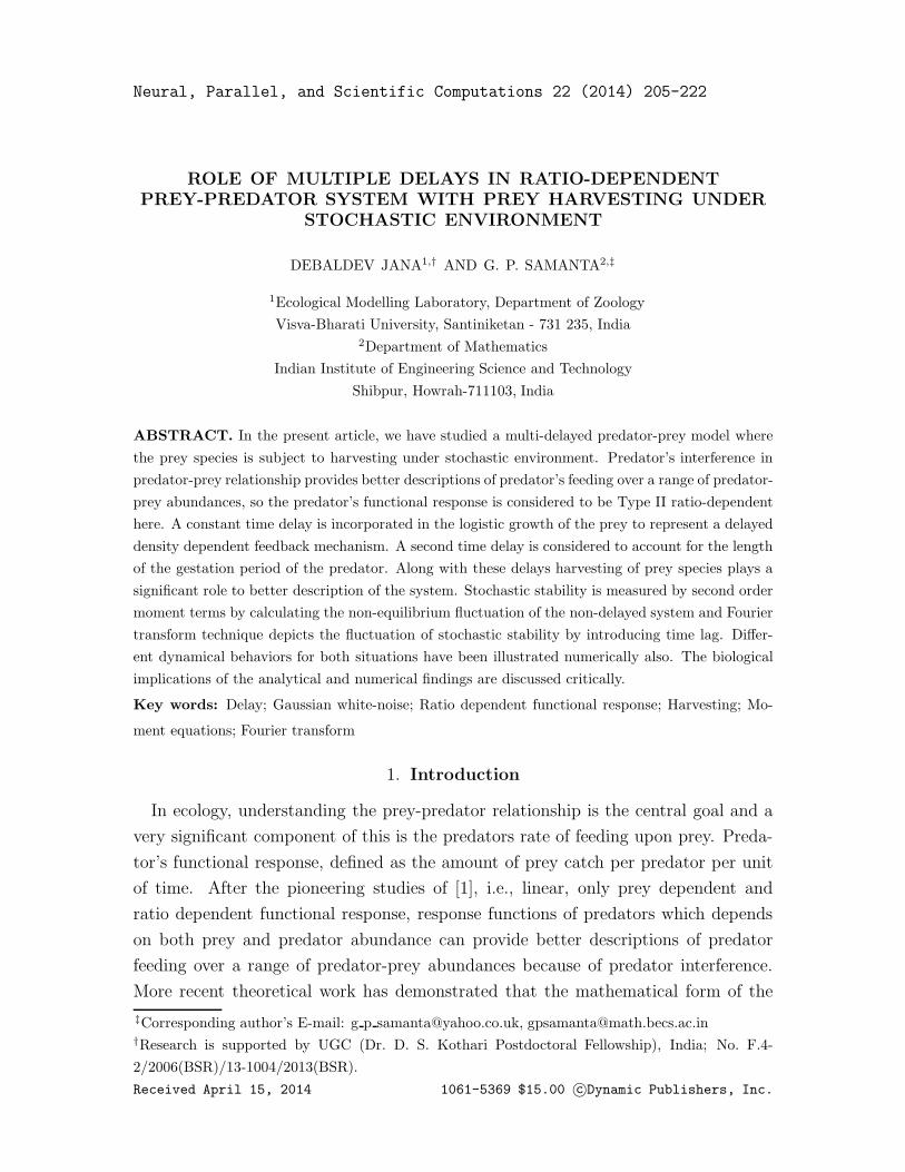
3.045 3.1 3.2 3.3 3.4 3.5 3.6 3.70
0.5
1
1.5
2
2.5
3
3.3
α
E
(A) ab0<1 (a=0.2, b
0=0.5)
R4R
2
R2 : H<0, A<0
R3
R1
R1 : H<0, A>0
R3 : H>0, A>0 & (3H)1/2<A
E* infeasible
R4 : H>0, A<0 & (3H)1/2<A
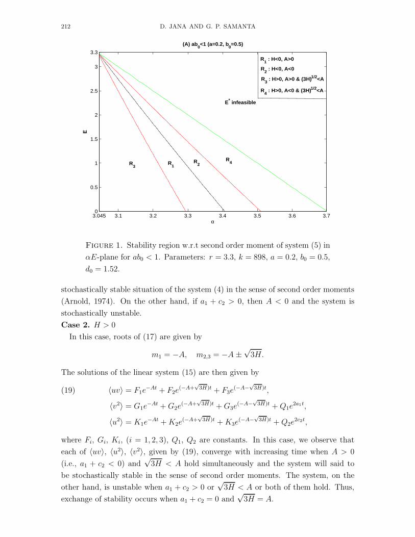
Figure 1. Stability region w.r.t second order moment of system (5) in
αE-plane for ab0 < 1. Parameters: r = 3.3, k = 898, a = 0.2, b0 = 0.5,
d0 = 1.52.
stochastically stable situation of the system (4) in the sense of second order moments
(Arnold, 1974). On the other hand, if a1 + c2 > 0, then A < 0 and the system is
stochastically unstable.
Case 2. H > 0
In this case, roots of (17) are given by
m1 = −A, m2,3 = −A ±√
3H.
The solutions of the linear system (15) are then given by
〈uv〉 = F1e−At + F2e
(−A+√
3H)t + F3e(−A−
√3H)t,(19)
〈v2〉 = G1e−At + G2e
(−A+√
3H)t + G3e(−A−
√3H)t + Q1e
2a1t,
〈u2〉 = K1e−At + K2e
(−A+√
3H)t + K3e(−A−
√3H)t + Q2e
2c2t,
where Fi, Gi, Ki, (i = 1, 2, 3), Q1, Q2 are constants. In this case, we observe that
each of 〈uv〉, 〈u2〉, 〈v2〉, given by (19), converge with increasing time when A > 0
(i.e., a1 + c2 < 0) and√
3H < A hold simultaneously and the system will said to
be stochastically stable in the sense of second order moments. The system, on the
other hand, is unstable when a1 + c2 > 0 or√
3H < A or both of them hold. Thus,
exchange of stability occurs when a1 + c2 = 0 and√
3H = A.
ROLE OF MULTIPLE DELAYS IN RATIO-DEPENDENT PREY-PREDATOR SYSTEM 213
0 10 20 30 40−0.5
0
0.5
1
1.5
2
2.5
3
Time
Sec
on
d o
rder
mo
men
ts
(i) α=3.3, E=0.5
0 5 10 15 20−5000
−4000
−3000
−2000
−1000
0
1000
2000
3000
4000
5000
Time
(iv) α=3.4, E=0.5
⟨u2⟩
⟨v2⟩
⟨uv⟩
⟨uv⟩
⟨v2⟩
⟨u2⟩
0 20 40 600
1
2
3
4
5
6
7
8
9
10
Time
Sec
on
d o
rder
mo
men
ts
(vii) α=3.15, E=0.5
0 1 2 3 40
100
200
300
400
500
600
700
800
900
1000
Time
(x) α=3.5, E=0.5
⟨u2⟩
⟨v2⟩
⟨v2⟩
⟨uv⟩
⟨u2⟩
⟨uv⟩
0 200 400 600 800 10000
50
100
150
200
x
(vi)
0 50 100 150 2000
200
400
600
800
1000
Time
(v)
0 100 200 300 400 5000
100
200
300
400
Time
Po
pu
lati
on
s
(ii)
0 100 200 300 4000
50
100
x
y
(iii)
x x
y
y
0 50 100 150 2000
200
400
600
800
1000
Time
Po
pu
lati
on
s
(viii)
0 200 400 600 800 10000
50
100
150
x
y
(ix)
0 200 400 600 8000
50
100
150
200
x
(xii)
0 50 100 150 2000
200
400
600
800
Time
(xi)
x
x
y y
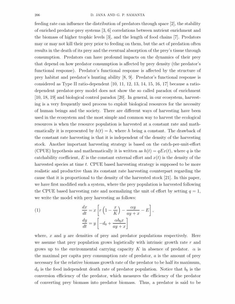
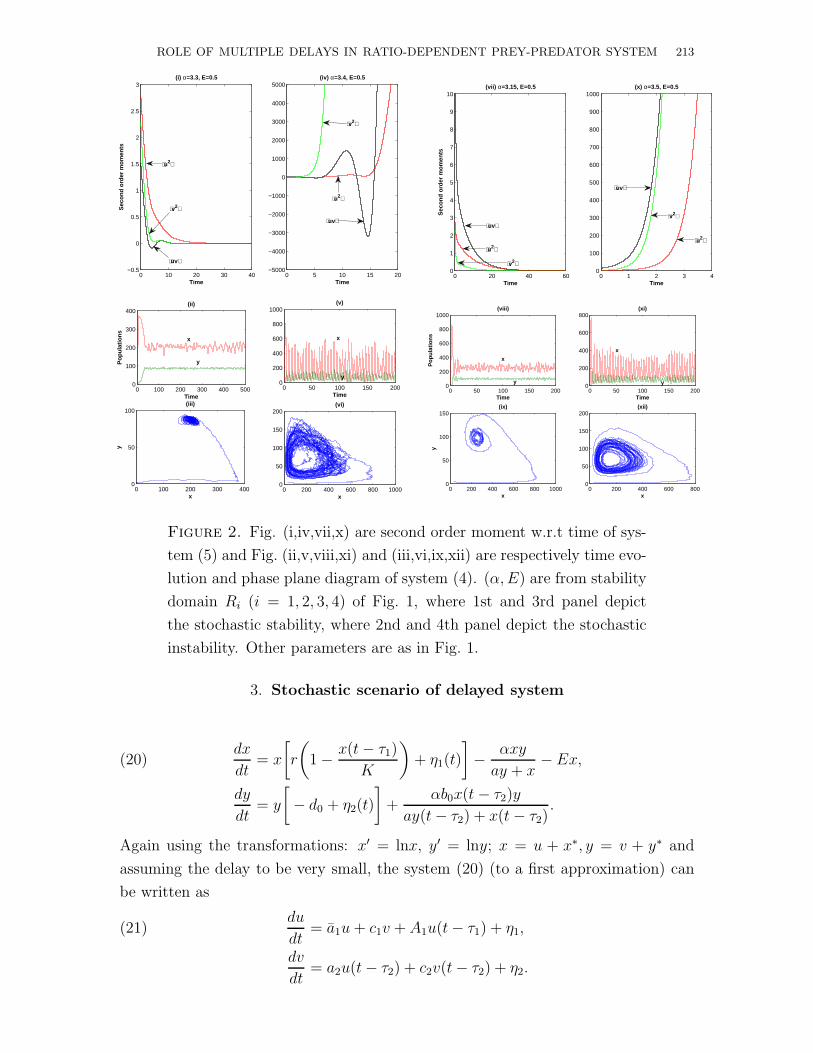
Figure 2. Fig. (i,iv,vii,x) are second order moment w.r.t time of sys-
tem (5) and Fig. (ii,v,viii,xi) and (iii,vi,ix,xii) are respectively time evo-
lution and phase plane diagram of system (4). (α, E) are from stability
domain Ri (i = 1, 2, 3, 4) of Fig. 1, where 1st and 3rd panel depict
the stochastic stability, where 2nd and 4th panel depict the stochastic
instability. Other parameters are as in Fig. 1.
3. Stochastic scenario of delayed system
dx
dt= x
[
r
(
1 − x(t − τ1)
K
)
+ η1(t)
]
− αxy
ay + x− Ex,(20)
dy
dt= y
[
− d0 + η2(t)
]
+αb0x(t − τ2)y
ay(t − τ2) + x(t − τ2).
Again using the transformations: x′ = lnx, y′ = lny; x = u + x∗, y = v + y∗ and
assuming the delay to be very small, the system (20) (to a first approximation) can
be written as
du
dt= a1u + c1v + A1u(t− τ1) + η1,(21)
dv
dt= a2u(t − τ2) + c2v(t − τ2) + η2.
214 D. JANA AND G. P. SAMANTA
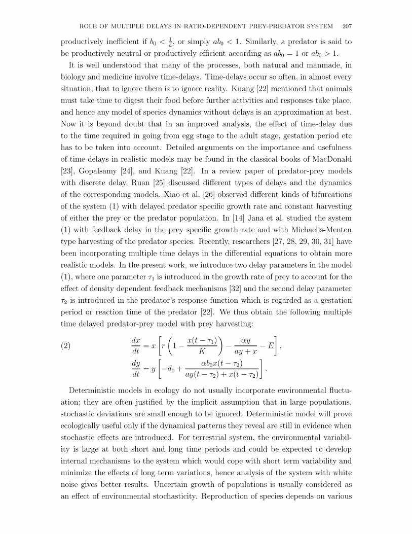
3.06 4 5 6 7 8 9 9.60
0.5
1
1.5
2
2.5
3
3.3
α
E
(B) ab0=1 (a=2, b
0=0.5)
R1 : H<0, A>0
R3 : H>0, A>0
& (3H)1/2<A
E* infeasible
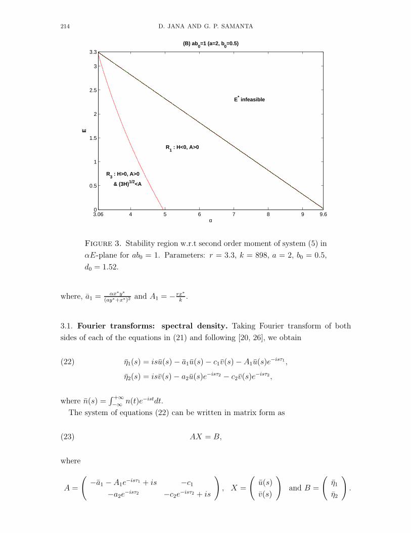
Figure 3. Stability region w.r.t second order moment of system (5) in
αE-plane for ab0 = 1. Parameters: r = 3.3, k = 898, a = 2, b0 = 0.5,
d0 = 1.52.
where, a1 = αx∗y∗
(ay∗+x∗)2and A1 = −rx∗
k.
3.1. Fourier transforms: spectral density. Taking Fourier transform of both
sides of each of the equations in (21) and following [20, 26], we obtain
η1(s) = isu(s) − a1u(s) − c1v(s) − A1u(s)e−isτ1 ,(22)
η2(s) = isv(s) − a2u(s)e−isτ2 − c2v(s)e−isτ2,
where n(s) =∫ +∞−∞ n(t)e−istdt.
The system of equations (22) can be written in matrix form as
(23) AX = B,
where
A =
(
−a1 − A1e−isτ1 + is −c1
−a2e−isτ2 −c2e
−isτ2 + is
)
, X =
(
u(s)
v(s)
)
and B =
(
η1
η2
)
.
ROLE OF MULTIPLE DELAYS IN RATIO-DEPENDENT PREY-PREDATOR SYSTEM 215
0 10 20 30 40−0.5
0
0.5
1
1.5
2
2.5
3
Time
Sec
on
d o
rder
mo
men
ts
(i) α=6, E=1
0 2 4 6 8 100
1
2
3
4
5
6
7
8
9
10
Time
(iv) α=4, E=1
⟨uv⟩
⟨uv⟩
⟨v2⟩
⟨u2⟩
⟨u2⟩
⟨v2⟩
0 100 200 300 400 5000
200
400
600
800
Time
Po
pu
lati
on
s(ii)
0 200 400 600 8000
20
40
60
x
y
(iii)
0 100 200 300 400 5000
200
400
600
800
Time
(v)
0 200 400 600 800 10000
50
100
150
x
(vi)
x x
y y
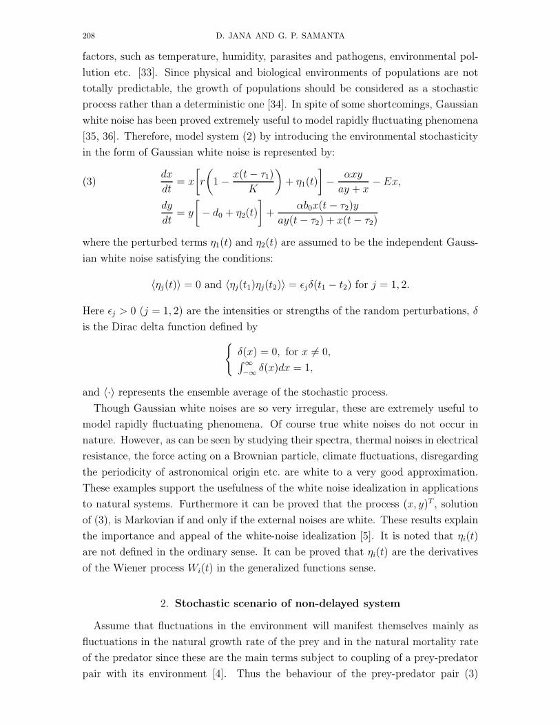
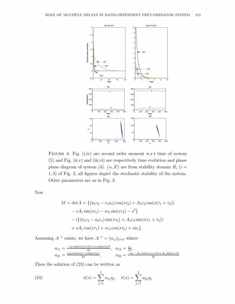
Figure 4. Fig. (i,iv) are second order moment w.r.t time of system
(5) and Fig. (ii,v) and (iii,vi) are respectively time evolution and phase
plane diagram of system (4). (α, E) are from stability domain Ri (i =
1, 3) of Fig. 3, all figures depict the stochastic stability of the system.
Other parameters are as in Fig. 3.
Now
M = detA = {(a1c2 − c1a2) cos(sτ2) + A1c2 cos(s(τ1 + τ2))
− sA1 sin(sτ1) − sc2 sin(sτ2) − s2}− i{(a1c2 − a2c1) sin(sτ2) + A1c2 sin(s(τ1 + τ2))
+ sA1 cos(sτ1) + sc2 cos(sτ2) + sa1}.
Assuming A−1 exists, we have A−1 = (aij)2×2, where
a11 = −c2 cos(sτ2)+i{s+c2 sin(sτ2)}M
, a12 = c1M
,
a21 = a2(cos(sτ2)−i sin(sτ2))M
, a22 = −a1−A1 cos(sτ1)+i{s+A1 sin(sτ1)}M
.
Then the solution of (23) can be written as
(24) u(s) =2∑
j=1
a1jηj , v(s) =2∑
j=1
a2jηj
216 D. JANA AND G. P. SAMANTA
3 4 5 6 7 8 9 10 11 12 130
0.5
1
1.5
2
2.5
3
3.3
α
E
(C) ab0>1 (a=3, b
0=0.5)
R1 : H<0, A>0
R3 : H>0, A>0
& (3H)1/2<A
R4 : H>0, A<0 & (3H)1/2<A
E* infeasible
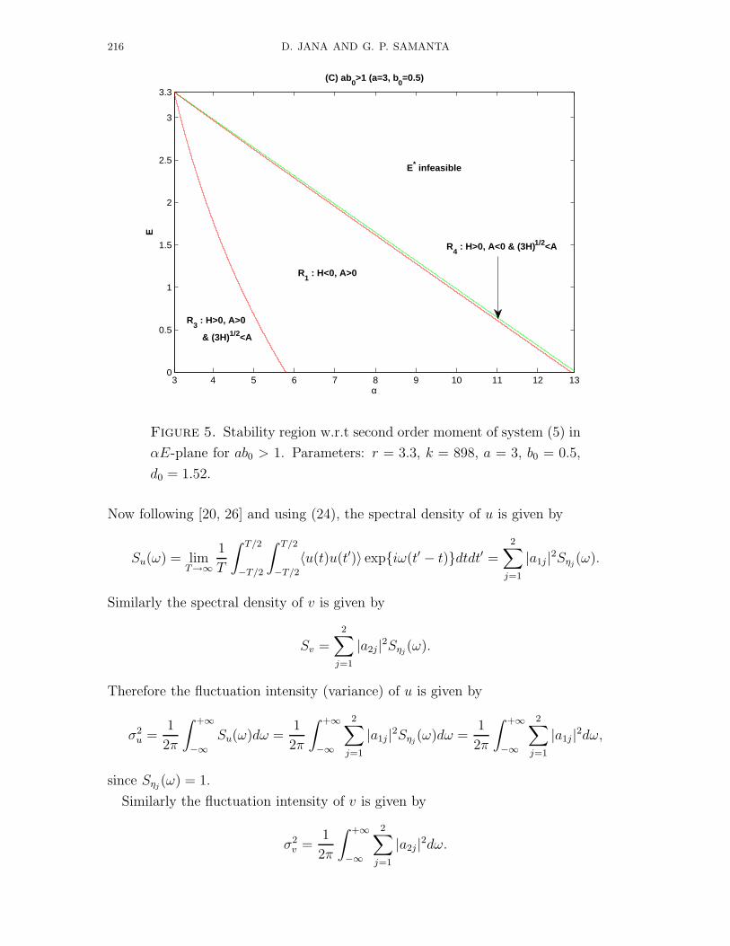
Figure 5. Stability region w.r.t second order moment of system (5) in
αE-plane for ab0 > 1. Parameters: r = 3.3, k = 898, a = 3, b0 = 0.5,
d0 = 1.52.
Now following [20, 26] and using (24), the spectral density of u is given by
Su(ω) = limT→∞
1
T
∫ T/2
−T/2
∫ T/2
−T/2
〈u(t)u(t′)〉 exp{iω(t′ − t)}dtdt′ =
2∑
j=1
|a1j |2Sηj(ω).
Similarly the spectral density of v is given by
Sv =
2∑
j=1
|a2j|2Sηj(ω).
Therefore the fluctuation intensity (variance) of u is given by
σ2u =
1
2π
∫ +∞
−∞Su(ω)dω =
1
2π
∫ +∞
−∞
2∑
j=1
|a1j |2Sηj(ω)dω =
1
2π
∫ +∞
−∞
2∑
j=1
|a1j |2dω,
since Sηj(ω) = 1.
Similarly the fluctuation intensity of v is given by
σ2v =
1
2π
∫ +∞
−∞
2∑
j=1
|a2j |2dω.
ROLE OF MULTIPLE DELAYS IN RATIO-DEPENDENT PREY-PREDATOR SYSTEM 217
0 0.5 1 1.5 2 2.5 3 3.5 4 4.5 5−2
0
2
4
6
8
10
12
14
16
Time
Sec
on
d o
rder
mo
men
ts
(i) α=7, E=1
⟨u2⟩ ⟨v2⟩
⟨uv⟩
0 2 4 6 8 100
5
10
15
Time
Sec
on
d o
rder
mo
men
ts
(iv) α=4, E=1
0 5 10 15 200
100
200
300
400
500
600
700
800
900
1000
Time
(vii) α=11, E=0.75
⟨u2⟩
⟨u2⟩
⟨v2⟩
⟨uv⟩⟨uv⟩
⟨v2⟩
0 20 40 60 80 1000
200
400
600
Time
Po
pu
lati
on
s
(ii)
0 200 400 6000
20
40
60
80
100(iii)
x
y
y
x
0 20 40 60 80 1000
50
100
150
200
250
Time
Po
pu
lati
on
s
(vii)
0 50 100 150 200 2500
50
100
150
200(ix)
x
y
0 20 40 60 80 1000
100
200
300
Time
(v)
0 100 200 3000
50
100(vi)
x
x
yy
x
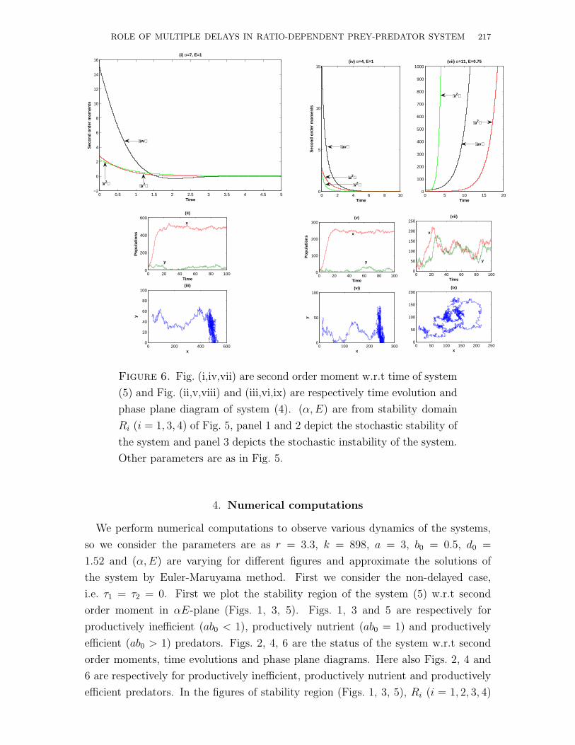
Figure 6. Fig. (i,iv,vii) are second order moment w.r.t time of system
(5) and Fig. (ii,v,viii) and (iii,vi,ix) are respectively time evolution and
phase plane diagram of system (4). (α, E) are from stability domain
Ri (i = 1, 3, 4) of Fig. 5, panel 1 and 2 depict the stochastic stability of
the system and panel 3 depicts the stochastic instability of the system.
Other parameters are as in Fig. 5.
4. Numerical computations
We perform numerical computations to observe various dynamics of the systems,
so we consider the parameters are as r = 3.3, k = 898, a = 3, b0 = 0.5, d0 =
1.52 and (α, E) are varying for different figures and approximate the solutions of
the system by Euler-Maruyama method. First we consider the non-delayed case,
i.e. τ1 = τ2 = 0. First we plot the stability region of the system (5) w.r.t second
order moment in αE-plane (Figs. 1, 3, 5). Figs. 1, 3 and 5 are respectively for
productively inefficient (ab0 < 1), productively nutrient (ab0 = 1) and productively
efficient (ab0 > 1) predators. Figs. 2, 4, 6 are the status of the system w.r.t second
order moments, time evolutions and phase plane diagrams. Here also Figs. 2, 4 and
6 are respectively for productively inefficient, productively nutrient and productively
efficient predators. In the figures of stability region (Figs. 1, 3, 5), Ri (i = 1, 2, 3, 4)
218 D. JANA AND G. P. SAMANTA
0 50 100 150 2000
200
400
600
800
1000
Time
Po
pu
lati
on
s
(i)
0 200 400 600 800 10000
50
100
150
200
x
y
(ii)
0 200 400 600 8000
50
100
150
200
x
(iv)
0 50 100 150 2000
200
400
600
800
Time
(iii)
x
x
y y
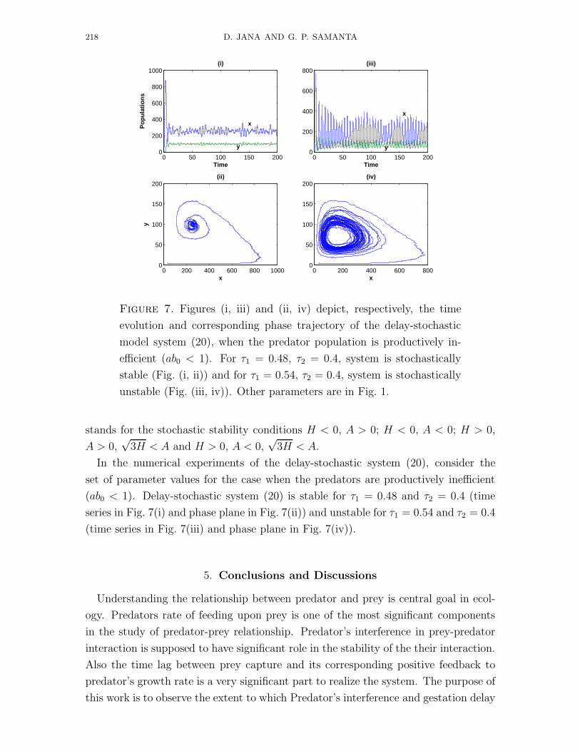
Figure 7. Figures (i, iii) and (ii, iv) depict, respectively, the time
evolution and corresponding phase trajectory of the delay-stochastic
model system (20), when the predator population is productively in-
efficient (ab0 < 1). For τ1 = 0.48, τ2 = 0.4, system is stochastically
stable (Fig. (i, ii)) and for τ1 = 0.54, τ2 = 0.4, system is stochastically
unstable (Fig. (iii, iv)). Other parameters are in Fig. 1.
stands for the stochastic stability conditions H < 0, A > 0; H < 0, A < 0; H > 0,
A > 0,√
3H < A and H > 0, A < 0,√
3H < A.
In the numerical experiments of the delay-stochastic system (20), consider the
set of parameter values for the case when the predators are productively inefficient
(ab0 < 1). Delay-stochastic system (20) is stable for τ1 = 0.48 and τ2 = 0.4 (time
series in Fig. 7(i) and phase plane in Fig. 7(ii)) and unstable for τ1 = 0.54 and τ2 = 0.4
(time series in Fig. 7(iii) and phase plane in Fig. 7(iv)).
5. Conclusions and Discussions
Understanding the relationship between predator and prey is central goal in ecol-
ogy. Predators rate of feeding upon prey is one of the most significant components
in the study of predator-prey relationship. Predator’s interference in prey-predator
interaction is supposed to have significant role in the stability of the their interaction.
Also the time lag between prey capture and its corresponding positive feedback to
predator’s growth rate is a very significant part to realize the system. The purpose of
this work is to observe the extent to which Predator’s interference and gestation delay
ROLE OF MULTIPLE DELAYS IN RATIO-DEPENDENT PREY-PREDATOR SYSTEM 219
drive the population dynamics of a predator-prey interaction under fluctuating envi-
ronment. Results shows that Predator’s interference plays a significant role to change
the stochastic stability of the system. To study the effect of environmental fluctuation
on the time-delayed predator-prey system (20), I have superimposed Gaussian white
noises on (2) and then study non-equilibrium fluctuation and stability of the resulting
stochastic model (20) by using Fourier transform technique. Following the criteria of
stability in the stochastic environment [43], it is seen that the environmental noises
have a destabilizing effect on the system. Also the deterministic system and the noise-
induced stochastic system may behave alike with respect to stability. It is well known
that natural populations of plants and animals neither increase indefinitely to blanket
the world nor become extinct (except in some rare cases due to some rare reasons).
Hence, in practice, we often want to keep the prey and predator population to an
acceptable level in finite time. In order to accomplish this we strongly suggest that
in realistic field situations (where effect of time-delay and environmental fluctuation
can never be violated), the parameters of the system should be regulated in such a
way that E∗ is deterministically stable.
REFERENCES
[1] C. S. Holling, Some characteristics of simple types of predation and parasitism. Canadian
Entomologist, 91, 385–398, 1959.
[2] J. van der Meer, B. J. Ens, Models of interference and their consequences for the spatial
distribution of ideal and free predators. Journal of Animal Ecology, 66, 846–858, 1997.
[3] D. L. DeAngelis, R. A. Goldstein, R. V. ONeill, A model for trophic interaction. Ecology, 56,
881–892, 1975.
[4] Dimentberg, M.F., Statistical Dynamics of Nonlinear and Time-Varying Systems, John Wiley
and Sons, New York, 1988.
[5] Horsthemke, W. and Lefever, R., Noise Induced Transitions, Springer-Verlag, Berlin, 1984.
[6] G. Huisman, R. J. De Boer, A formal derivation of the ”Beddington” functional response.
Journal of Theoretical Biology, 185, 389–400, 1997.
[7] Schmitz, O. J., 1992. Exploitation in model food chains with mechanistic consumerresource
dynamics. Theoretical Population Biology, 41, 161–183.
[8] Alstad, D., 2001. Basic Populas Models of Ecology. Prentice Hall, Inc., NJ.
[9] Anderson, O., 1984. Optimal Foraging by largemouth bass in structured environments. Ecol-
ogy. 65, 851–861.
[10] Kuang, Y., Beretta, E., 1998. Global qualitative analysis of a ratio-dependent predator-prey
system. J. Math. Biol., 36, 389–406.
[11] Martin, A., Ruan, S., 2001. Predator-prey models with delay and prey harvesting. J. of Math.
Biol. 43(3), 247–267.
[12] Jost, C., Arino, O., Arditi, R., 1999. About deterministic extinction in ratio-dependent
predator-prey models. Bull. Math. Biol. 61, 19–32.
[13] Xiao, D., Ruan, S., 2001. Global dynamics of a ratio-dependent predator-prey system. J. Math.
Biol. 43, 268–290.
220 D. JANA AND G. P. SAMANTA
[14] Jana, D., Chakraborty, S., Bairagi, N., 2012. Stability, Nonlinear Oscillations and Bifurcation
in a Delay-Induced Predator-Prey System with Harvesting. Engineering Letters, 20(3), 238–
246.
[15] Xiao, D., Jennings, L. S., Bifurcations of a ratio-dependent predator-prey system with constant
rate harvesting. SIAM J. Appl. Math. Biol., 659(3), 737–753, (2005).
[16] Xiao, D., Li, W., Han, M., 2006. Dynamics of a ratio-dependent predator-prey model with
predator harvesting. J. Math. Anal. Appl. 324, 14–29.
[17] Chakraborty, S., Pal, S. and Bairagi, N. (2012). Predator-prey interaction with harvesting -
mathematical study with biological ramifications. Applied Mathematical Modelling, 36, 4044–
4059.
[18] Hairston, N.G., Smith, F.E., Slobodkin, L.B., 1960. Community structure, population control
and competition. American Naturalist 94, 421–425.
[19] Rosenzweig, M.L., 1969. Paradox of Enrichment: destabilization of exploitation systems in
ecological time. Science 171, 385–387.
[20] Luck, R.F., 1990. Evaluation of natural enemies for biological control: a behavior approach.
Trends in Ecology and Evolution 5, 196–199.
[21] Clark C.W. (1976) Mathematical Bioeconomics: The optimal Management of Renewable Re-
sources. John Wiley & Sons, New York.
[22] Kuang Y., Delay Differential Equations with Applications in Population Dynamics, Academic
Press, New York, 1993.
[23] Macdonald N., Biological Delay Systems: Linear Stability Theory, Cambridge University Press,
Cambridge, 1989.
[24] Gopalsamy K., Stability and Oscillations in Delay Differential Equations of Population Dy-
namics, Kluwer Academic, Dordrecht,1992.
[25] Ruan, S. (2009) On Nonlinear Dynamics of Predator-Prey Models with Discrete Delay. Math.
Model. Nat. Phenom., 4(2), 140–188.
[26] Xia, J., Liu, Z. Yuan, R. and Ruan, S. (2009) The effects of harvesting and time delay on
predator-prey systems with Holling Type II functional response. SIAM J. Appl. Math., 70(4),
1178–1200.
[27] Hu, G.P., Li, W.T. and Yan, X.P. (2009) Hopf bifuractation in a delayed predator-prey system
with multiple delays. Chaos Soli. Frac., 42, 1273–1285.
[28] Liao, M., Tang, X. and Xu, C. (2012) Bifurcation analysis for a three-species predator-prey
system with two delays. Commun Nonlinear Sci Numer Simulat., 17, 183–194.
[29] Meng, X.Y., Huo, H.F. and Zhang, X.B. (2011) Stability and global Hopf bifurcation in a
delayed food web consisting of a prey and two predators. Commun Nonlinear Sci Numer
Simulat., 16, 4335–4348.
[30] Song, Y.L., Peng, Y.H. and Wei, J.J. (2008) Bifurcations for a predator-prey system with two
delays. J. Math. Anal. Appl., 337, 466–79.
[31] Yan, X.P. and Chu, Y.D. (2006) Stability and bifurcation analysis for a delayed Lotka-Volterra
predator-prey system. Journal of Computational and Applied Math., 196, 198–210.
[32] Freedman, H.I. (1987) Deterministic Mathematical Models in Population Ecology. HIFR Con-
sulting Ltd., Edmonton.
[33] Y. Iwasa, H. Hakoyama, M. Nakamaru, J. Nakanishi, Estimate of population extinction risk
and its application to ecological risk management, Popul Ecol 42 (2000), pp. 73–80.
[34] M. Turelli, Stochastic Community Theory: A Partially Guided Tour, In Mathematical Ecology,
edited. by Hallman TG, Levin S, Springer-Verlag, Berlin, 1986.
ROLE OF MULTIPLE DELAYS IN RATIO-DEPENDENT PREY-PREDATOR SYSTEM 221
[35] M. C. Valsakumar, K. P. N. Murthy, G. Ananthakrishna, On the linearization of non-linear
Langevin type stochastic differential equations, J. Stat. Phys 30 (1983), pp. 617–631.
[36] G. P. Samanta, A. Maiti, Stochastic Gomatam model of interacting species: non-equilibrium
fluctuation and stability, Syst. Anal. Model. Sim. 43 (2003), pp. 683–692.
[37] Y. Kuang, H. I. Freedman, Uniqueness of limit cycles in Gause-type models of predator-prey
systems, Math. Biosci. 88 (1988), pp. 67–84.
[38] J. E. Marsden, M. McCracken, The Hopf Bifurcation and its application, Springer-Verlag, New
York, 1976.
[39] N. G. Van Kampen, Stochastic process in Physics and Chemistry, North Holland Publishing
Co, Amsterdam, 1981.
[40] M. Bandyopadhyay and C. G. Chakraborti, Deterministic and stochastic analysis of a non-
linear prey-predator system, J. Biol. Syst. 11 (2003), pp. 161–172.
[41] M. C. Baishya and C. G. Chakraborti, Non-equilibrium fluctuation in Lotka-Volterra system,
B. Math. Biol. 49 (1987), pp. 125–131.
[42] G. Nikolis, L. Prigogine, Self-Organization in Non-Equilibrium Systems, Wiely, New York,
1977.
[43] R. M. May, Stability and Complexity in Model Ecosystems. Princeton University Press, Prince-
ton, 1974.