Sandom, C., L. Dalby, C. Fløjgaard, W. D. Kissling, J. Lenoir, B. Sandel, K. Trøjelsgaard, R.

Ejrnæs, and J.C. Svenning (Submitted) Mammal predator and prey species richness are

strongly linked at macroscales. Ecology.

Appendix A. Supplementary results recording spatial autocorrelation analysis.

Figure A1 Correlograms of a series of independent ordinary least square (OLS) regression models

for example, one model predicting NDVI from PC1–PC3, one predicting prey richness from PC1–

PC3 and NDVI, and one predicting predator richness from PC1–PC3, NDVI and prey richness) run

to assess the degree of spatial autocorrelation in SEM residual.

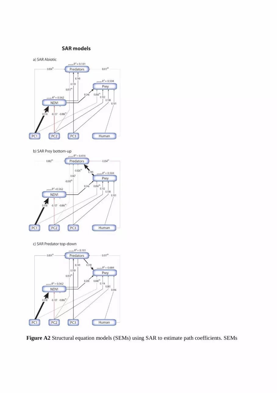
Figure A2 Structural equation models (SEMs) using SAR to estimate path coefficients. SEMs

represent direct and indirect effects of climate (PC1–PC3), productivity (NDVI) and human

influence (Human) on predator and prey diversity and their associations. Three types of SEMs are

represented: (a) abiotic SEMs without a direct link between predators and prey, (b) bottom-up

SEMs including a direct link from prey to predator diversity, and (c) a top-down SEM including a

direct link from predator to prey diversity. Figure panels represent global SEMs across all species.

Black arrows represent positive path coefficients and red negative, with line thickness being

proportional to coefficient strength.

Appendix B. Supplementary results recording full SEM path coeffients for each biogeographic

realm.

Tables A-C A comparison of all path coefficients for the abiotic (Table A), bottom-up (Table B)

and top-down (Table C) SEMs for each of the biogeographic realms analysed. Arrows (->) indicate

the direction of the path coefficients between two variables. A dashed line (--) indicates error co-

variances representing unanalyzed relationships between exogenous variables. ‘NA’ indicates the

link was not included within the model.

Table A

Abiotic Afrotropics Australia Indo-Malay Nearctic Neotropics Palearctic

NDVI->Prey 0.527 0.294 0.524 0.796 0.424 0.359

Human-> Prey

0.075 0.139 -0.217 0.089 0.053 0.365

PC1->Prey 0.204 -0.479 -0.053 0.146 -0.306 -0.339

PC2->Prey 0.196 0.260 0.118 -0.589 -0.318 0.018

PC3->Prey -0.014 -0.231 -0.145 -0.228 -0.200 -0.300

NDVI-> Predators

0.513 0.634 0.425 1.118 0.361 0.176

Human-> Predators

0.216 0.074 -0.006 -0.211 -0.142 0.255

PC1-> Predators

-0.695 0.421 0.218 -0.485 -0.169 -0.240

PC2-> Predators

0.339 0.317 0.446 -0.606 -0.282 -0.029

PC3-> Predators

-0.019 -0.338 -0.082 -0.481 -0.218 -0.462

PC1->NDVI 0.906 -0.804 -0.856 0.561 -0.790 -0.368

PC2->NDVI 0.004 -0.316 0.074 0.284 0.217 -0.430

PC3->NDVI 0.218 0.193 0.036 0.427 0.018 0.477

Human--NDVI

NA 0.126 -0.113 0.118 0.094 0.220

Prey--Prey 0.401 0.322 0.430 0.143 0.449 0.413

Predators--Predators

0.779 0.834 0.691 0.400 0.620 0.668

NDVI--NDVI 0.131 0.216 0.259 0.422 0.332 0.452

Predators--Prey

0.347 0.108 0.410 0.110 0.371 0.395

Human--Human

0.998 0.996 0.996 0.998 0.998 0.999

PC1--Human 0.414 -0.473 0.589 0.663 0.356 -0.187

PC2--Human 0.038 -0.533 NA 0.148 NA -0.508

PC3--Human -0.192 0.242 NA 0.419 -0.167 0.367

PC1--PC1 0.998 0.996 0.996 0.998 0.998 0.999

PC2--PC1 <0.001 NA NA NA NA NA

PC3--PC1 <0.001 NA NA NA NA NA

PC2--PC2 0.998 0.996 0.996 0.998 0.998 0.999

PC3--PC2 <0.001 NA <0.001 NA NA NA

PC3--PC3 0.998 0.996 0.996 0.998 0.998 0.999

Table B

Bottom-up Afrotropics Australia Indo-Malay Nearctic Neotropics Palearctic

Prey-> Predators

0.865 0.336 0.955 0.771 0.826 0.957

NDVI-> Predators

0.058 0.536 -0.075 0.504 0.011 -0.168

Human-> Predators

0.151 0.027 0.201 -0.279 -0.186 -0.094

PC1-> Predators

-0.871 0.583 0.269 -0.597 0.084 0.085

PC2-> Predators

0.169 0.230 0.334 -0.152 -0.019 -0.046

PC3-> Predators

-0.007 -0.261 0.057 -0.305 -0.053 -0.175

NDVI->Prey 0.527 0.294 0.524 0.796 0.424 0.359

Human-> Prey

0.075 0.139 -0.217 0.089 0.053 0.365

PC1->Prey 0.204 -0.479 -0.053 0.146 -0.306 -0.339

PC2->Prey 0.196 0.260 0.118 -0.589 -0.318 0.018

PC3->Prey -0.014 -0.231 -0.145 -0.228 -0.200 -0.300

PC1->NDVI 0.906 -0.804 -0.856 0.561 -0.790 -0.368

PC2->NDVI 0.004 -0.316 0.074 0.284 0.217 -0.430

PC3->NDVI 0.218 0.193 0.036 0.427 0.018 0.477

Human--NDVI

NA 0.126 -0.113 0.118 0.094 0.220

Predators--Predators

0.479 0.798 0.300 0.315 0.314 0.290

Prey--Prey 0.401 0.322 0.430 0.143 0.449 0.413

NDVI--NDVI 0.131 0.216 0.259 0.422 0.332 0.452

Human--Human

0.998 0.996 0.996 0.998 0.998 0.999

PC1--Human 0.414 -0.473 0.589 0.663 0.356 -0.187

PC2--Human 0.038 -0.533 NA 0.148 NA -0.508

PC3--Human -0.192 0.242 NA 0.419 -0.167 0.367

PC1--PC1 0.998 0.996 0.996 0.998 0.998 0.999

PC2--PC1 <0.001 NA NA NA NA NA

PC3--PC1 <0.001 NA NA NA NA NA

PC2--PC2 0.998 0.996 0.996 0.998 0.998 0.999

PC3--PC2 <0.001 NA <0.001 NA NA NA

PC3--PC3 0.998 0.996 0.996 0.998 0.998 0.999

Table C

Top-down Afrotropics Australia Indo-Malay Nearctic Neotropics Palearctic

Predators-> Prey

0.445 0.130 0.593 0.275 0.598 0.592

NDVI->Prey 0.299 0.211 0.272 0.488 0.208 0.255

Human-> Prey

-0.021 0.130 -0.214 0.147 0.138 0.214

PC1->Prey 0.513 -0.534 -0.183 0.279 -0.205 -0.197

PC2->Prey 0.045 0.219 -0.147 -0.423 -0.149 0.035

PC3->Prey -0.005 -0.187 -0.097 -0.096 -0.070 -0.026

NDVI-> Predators

0.513 0.634 0.425 1.118 0.361 0.176

Human-> Predators

0.216 0.074 -0.006 -0.211 -0.142 0.255

PC1-> Predators

-0.695 0.421 0.218 -0.485 -0.169 -0.240

PC2-> Predators

0.339 0.317 0.446 -0.606 -0.282 -0.029

PC3-> Predators

-0.019 -0.338 -0.082 -0.481 -0.218 -0.462

PC1->NDVI 0.906 -0.804 -0.856 0.561 -0.790 -0.368

PC2->NDVI 0.004 -0.316 0.074 0.284 0.217 -0.430

PC3->NDVI 0.218 0.193 0.036 0.427 0.018 0.477

Human--NDVI NA 0.126 -0.113 0.118 0.094 0.220

Prey--Prey 0.247 0.308 0.186 0.113 0.227 0.179

Predators--Predators

0.779 0.834 0.691 0.400 0.620 0.668

NDVI--NDVI 0.131 0.216 0.259 0.422 0.332 0.452

Human--Human

0.998 0.996 0.996 0.998 0.998 0.999

PC1--Human 0.414 -0.473 0.589 0.663 0.356 -0.187

PC2--Human 0.038 -0.533 NA 0.148 NA -0.508

PC3--Human -0.192 0.242 NA 0.419 -0.167 0.367

PC1--PC1 0.998 0.996 0.996 0.998 0.998 0.999

PC2--PC1 <0.001 NA NA NA NA NA

PC3--PC1 <0.001 NA NA NA NA NA

PC2--PC2 0.998 0.996 0.996 0.998 0.998 0.999

PC3--PC2 <0.001 NA <0.001 NA NA NA

PC3--PC3 0.998 0.996 0.996 0.998 0.998 0.999

Appendix C. Supplementary results recording prey to predator ratios.

Figure C1. Ratio of prey to predator richness. Grid represents Behrmann projection (a cylindrical

equal area projection) with a resolution of two degree equivalents. Grid cells with less than 50%

land cover or those covering Antarctica were removed.