a quasi chemical approach for the modeling of predator-prey interactions
TRANSCRIPT
Network Biology, 2014, 4(3): 130-150
IAEES www.iaees.org
Article
A quasi chemical approach for the modeling of predator-prey
interactions Muhammad Shakil1, H. A. Wahab1, Muhammad Naeem2, Saira Bhatti3 1Department of Mathematics, Hazara University, Manshera, Pakistan 2Department of Information Technology, Hazara University, Manshera, Pakistan 3Department of Mathematics, COMSATS Institute of Information Technology, Abbottabad, Pakistan
E-mail: [email protected],[email protected]
Received 3 April 2014; Accepted 8 May 2014; Published online 1 September 2014
Abstract
We aim to develop the reaction diffusion equation for different types of mechanism of the predator-prey
interactions with quasi chemical approach. The chemical reactions representing the interactions obey the mass
action law. Since the cell-jump models may be considered as the proper diffusion models by themselves, the
territorial animal like fox is given a simple cell as its territory. Under the proper relations between coefficients,
like complex balance or detailed balance, this system demonstrated globally stable dynamics.
Keywords quasi-chemical approach; predator-prey interactions; modeling fox and rabbit interactions.
1 Introduction
The Lotka Voltera equations are a pair of first order non linear differential equations these are also known as the
predator prey equations .i.e. when the growth rate of one population is decreased and the other increased then the
populations are in a predator-prey situation. The Lotka–Volterra equations are frequently used to describe the
dynamics of biological in which two species interact, one as a predator and the other as prey.
In this review paper, we aim to study the interactions between the territorial animals like foxes and the
rabbits. The territories for the foxes are considered to be the simple cells. The interactions between predator
and its prey are represented by the chemical reactions which obey the mass action law. In this sence, we aim to
study the mass action law for Lotka-Volterra predator prey models and consider the quasi chemical approach
for the interactions between the predator and its prey. We also aim to develop the reaction diffusion equation
for different types of mechanism of the predator prey interactions. The principle of detailed balance, however
can also be introduced in some cases. Since the cell-jump models may be considered as the proper diffusion
models by themselves, the territorial animal like fox is given a simple cell as its territory. The sense in which
the discrete equations for cells converge to the partial differential equations of diffusion is that the cell models
Network Biology ISSN 22208879 URL: http://www.iaees.org/publications/journals/nb/onlineversion.asp RSS: http://www.iaees.org/publications/journals/nb/rss.xml Email: [email protected] EditorinChief: WenJun Zhang Publisher: International Academy of Ecology and Environmental Sciences
Network Biology, 2014, 4(3): 130-150
IAEES www.iaees.org
give the semi-discrete approximation of the partial differential equations for diffusion which result in a system
of ordinary differential equations in cells. There are jumps of concentrations on the boundary of cells. The
system of semi discrete models for cells with “no-flux” boundary conditions has all the nice properties of the
chemical kinetic equations for closed systems. Under the proper relations between coefficients, like complex
balance or detailed balance, this system demonstrated globally stable dynamics.
Here in this review paper, we will give background of the development of the different models of
Lotka-Volterra types of reaction-diffusion equation along with different approaches that were acquired by the
different scientist in the ecology and mathematical biology. Then we come to our goals, where we borrowed
the properties of the chemical reactions for our approach to develop the reaction-diffusion equation of Lotka
Volterra type.
The Lotka Volterra predator prey models were originally introduced by Alfred J. Lotka (1920) in the
theory of autocatalytic chemical reactions in 1910 this was effectively the logistic equation which was
originally derived by Pierre Francois Verhulst. In 1920 Lotka extended the model to "organic systems" using a
plant species and an herbivorous animal species as an example and in 1925 he utilized the equations to analyze
predator-prey interactions in his book on biomathematics arriving at the equations that we know today.
In 1926, Vito Volterra (Voltera, 1926), made a statistical analysis of fish catches in the Adriatic
independently investigated the equations. V. Voltera applied these equations to predator prey interactions;
consist of a pair of first order autonomous ordinary differential equations.
Since that time the Lotka–Voltera model has been applied to problems in chemical kinetics, population
biology, epidemiology and neural networks. These equations also model the dynamic behavior of an arbitrary
number of competitors. The Lotka–Volterra system of equations is an example of a Kolmogorov model, which
is a more general framework that can model the dynamics of ecological systems with predator-prey
interactions, competition, disease, and mutualism.
Lotka Volterra is the most famous predator prey model. According to Volterra if ( )x t is the prey
population and ( )y t that of the predator at time t then Volterra’s model is (Murray, 2003),
( )dx
x a bydt
(1)
( )dy
y cx ddt
(2)
where a, b, c and d are positive constants. Often some necessary modifications are possible here e.g. for an
absent predator a limited growth of prey can be introduced. The assumptions in the model are:
In the absence of any predation the prey grows unboundedly in a Malthusian way; this is the ax term
in equation (1).
The effect of the predation is to reduce the prey’s per capita growth rate by a term proportional to the prey
and predator populations; this is the bxy term.
In the absence of any prey for sustenance the predator’s death rate results in exponential decay, that is, the
dy term in equation (2).
The prey’s contribution to the predators’ growth rate is cxy ; i.e. it is proportional to the available prey as
well as to the size of the predator population.
The xy terms are representing the conversion of energy from one source to another.
bxy is taken from the prey and cxy accrues to the predators.
131
Network Biology, 2014, 4(3): 130-150
IAEES www.iaees.org
The model (1) and (2) are known as the Lotka–Volterra model but this model has serious drawbacks.
Nevertheless it has been of considerable value in posing highly relevant questions and is a jumping-off place
for more realistic models; this is the main motivation of study here (Murray, 2003).
2 Interacting Population Models
The population dynamics of each species is affected whenever two or more species interact. Generally there
consist whole webs of interacting species; those webs which consist structurally for complex communities are
called a trophic web. The dynamics outcomes of the interactions are very sensitive to initial data and parameter
values. The interactions lead to the following possible outcomes,
Competitive exclusion;
Total extinction, i.e., collapse of the whole system;
Coexistence in the form of positive steady state;
Coexistence in the form of oscillatory solutions;
A better and friendly competitor can save a otherwise doomed prey species.
Two or more species models consist in case of concentrating particularly on two-species systems. There are
three main types of interactions.
If the growth rate of one population is decreased and the other increased the populations are in a
predator–prey situation.
If the growth rate of each population is decreased then it is competition.
If each population’s growth rate is enhanced then it is called mutualism or symbiosis (Murray, 2003).
3 The Effect of Complexity on Stability
To explain the relationship between structural complexity and stability of ecosystems an extensive literature is
available. Theoretical study reviews shows that the term stability is mostly used to mean the condition that
whereby species densities, when perturbed from equilibrium, again return to that equilibrium. Analytically this
condition can be made tractable by assuming that the populations are perturbed slightly so that linear
approximations can be made to the nonlinear equations.
To know the effect of complexity on stability briefly let us take the generalized Lotka–Volterra
predator–prey system where there are n prey species and n predators, which prey on all the prey species
but with different severity. Then in place of (1) and (2) it can be written as,
1
1
ni
i i ij jj
ni
i ij j ij
dxx a b y
dt
dyy c x d
dt
1,2,3,...,i n (3)
and all of the , ,i ij ij ia b c and d are positive constants (Murray, 2003).
4 Realistic Predator–Prey Models
Though the Lotka–Volterra model is unrealistic because one of the unrealistic assumption is that growth of the
prey population is unbounded in the absence of predation and the other is that there is no limit to the prey
consumption but it suggests that simple predator–prey interactions can result in periodic behaviour of the
populations. Since it is not unexpected that if a prey population increases then it encourages growth of its
predator and more predators consume more prey due to which its population starts to decline. With the less
132
Network Biology, 2014, 4(3): 130-150
IAEES www.iaees.org
food around the predator population declines and when it is low enough, this allows the prey population to
increase and the whole cycle starts over again. Depending on the detailed system such oscillations can grow or
decay or go into a stable limit cycle oscillation or even exhibit chaotic behaviour, although in the latter case
there must be at least three interacting species, or the model has to have some delay terms. A limit cycle
solution is a closed trajectory in the predator–prey space which is not a member of a continuous family of
closed trajectories. A stable limit cycle trajectory is such that any small perturbation from the trajectory decays
to zero.
One of the unrealistic assumptions in the Lotka–Volterra models, (1) and (2), and generally (3), is that the
prey growth is unbounded in the absence of predation.
In the form we have written the model (1) and (2) the bracketed terms on the right are the
density-dependent per capita growth rates. To be more realistic these growth rates should depend on both the
prey and predator densities as,
( , ), ( , ).dx dy
x F x y y G x ydt dt
(4)
where the forms of F and G depend on the interaction, the species and so on. A more realistic prey
population equation might take the form,
( , ), ( , ) 1 ( ).dx x
x F x y F x y r y R xdt k
(5)
where ( )R x is one of the predation term and K is the constant carrying capacity for the prey when 0.P
The predator population equation, the second of (5), should also be made more realistic than simply having
G d cx as in the Lotka–Volterra model (2). Possible forms are,
( , ) 1 , ( , ) ( )hy
G x y k G x y d eR xx
(6)
where k, h, d and e are positive constants. The first of (6) says that the carrying capacity for the predator is
directly proportional to the prey density (Murray, 2003).
5 Competitioning Models
Here, for a common food source two species compete to each other. For example, competition may be for
territory which is directly related to food resources. Mathematically, carrying capacity of one species is
reduced by the other species and vice versa. When two or more species compete for the same limited food
source or in some way inhibit each other’s growth, a very simple competition model which demonstrates a
fairly general principle which is observed to hold in nature is that in the competition for the same limited
resources one of the species usually becomes extinct. The basic two species Lotka–Volterra competition model
with each species 1n and 2n have logistic growth in the absence of the other. Inclusion of logistic growth in
the Lotka–Volterra systems makes them much more realistic, but to highlight the principle the simpler model
which nevertheless reflects many of the properties of more complicated models, particularly as regards
stability.
1 1 21 1 12
1 1
1dx x x
r x bdt k k
(7)
133
Network Biology, 2014, 4(3): 130-150
IAEES www.iaees.org
2 2 12 2 21
2 2
1dx x x
r x bdt k k
(8)
where 1 1 2, 2, 12, ,r k r k b and 21b are positive constants and r’s are the linear birth rates and the k’s are the
carrying capacities. The 12b and 21b measure the competitive effect of 2n on 1n and 1n on 2n respectively
and they are not equal generally (Murray, 2003).
Note that the competition models (7) and (8) are not a conservative system like its Lotka–Volterra
predator–prey counterpart and if we non dimensionalise this model by writing
1 2 11 2 1
1 2 1
2 112 12 21 21
1 2
, , , ,
,
t
x x ru u r
k k r
k ka b a b
k k
(9)
(6) and (8) become
11 1 12 2 1 1 2
22 2 21 1 2 1 2
(1 ) ( , ),
(1 ) ( , ),
duu u a u f u u
ddu
pu u a u f u ud
(10)
The steady states, and phase plane singularities are the solutions of 1 1 2 2 1 2( , ) ( , ) 0f u u f u u (Murray,
2003).
6 Mutualism or Symbiosis
In these cases, the two species benefit from each other. To some extent it is the opposite of the competition
model here carrying capacity of each species is increased by the other species.
There are many cases where the interaction of two or more species is to the advantage of all. In promoting
and even in maintaining such species mutualism or symbiosis often plays a very crucial role. Plant and seed
dispersal is an example. If the survival is not at stake even in those situations the advantage of mutualism or
symbiosis can have its own importance. As a topic of theoretical ecology, even for two species, this area has
not been as widely studied as the others even though its importance is comparable to that of predator–prey and
competition interactions (Lotka, 1920). This is in part due to the fact that simple models in the Lotka–Volterra
vein give silly results. The simplest mutualism model equivalent to the classical Lotka–Volterra predator–prey
one is,
1 21 1 1 1 2 2 2 2 2 1. ,
dx dnr x a x x r n a n n
dt dt
where 1 2 1 2, ,r r a and a are positive constants.
Since 1 0dx
dt and 2 0,
dx
dt 1n and 2n simply grow unboundedly (Murray, 2003).
7 Threshold Phenomena
With the exception of the Lotka–Volterra predator–prey model, the two species models, which have either a
134
Network Biology, 2014, 4(3): 130-150
IAEES www.iaees.org
stable steady states where small perturbations die out, or unstable steady states where perturbations from them
grow unboundedly or result is produced in limit cycle periodic solutions. There is an interesting group of
models which have a nonzero stable state such that if the perturbation is sufficiently large or it is of the right
kind, then before returning to the steady state population densities undergo large variations. Such models are
said to exhibit a threshold effect (Murray, 2003). One such group of models is studied here. The model
predator–prey system is
( ) ( , ),
( ) ( , )
dxx F x y f x y
dtdy
y x G y g x ydt
(11)
where for convenience all the parameters have been incorporated in the F and G by a suitable rescaling.
8 Discrete Growth Models for Interacting Populations
Now taking the two interacting species, each have the non overlapping generations and each species affect the
other’s population dynamics. In the continuous growth models, there are some main types of interaction, such
as, predator–prey, mutualism and competition. Nowhere near to the same extent as for continuous models for
which, in the case of two species, there is a complete mathematical treatment of the equations. In view of the
complexity of solution behaviour with single-species discrete models it is not surprising that even more
complex behaviour is possible with coupled discrete systems (Murray, 2003).
The interaction between the prey ( )x and the predator ( )y to be governed by the discrete time (t)
system of coupled equations as,
1 , ,( )t t t tx rx f yx (12)
1 g( ,),t t t txy x y (13)
where r > 0 is the net linear rate of increase of the prey and f and g are functions which relate the
predator-influenced reproductive efficiency of the prey and the searching efficiency of the predator
respectively.
9 Detailed Analysis to Predator Prey Models
Predator-dependent predator-prey model is of the form
( , ), (0) 0,
( , ) , (0) 0,
dx xxg yP x y x
dt k
dycyP x y dy y
dt
(14)
when ,x
P x yy
then model (14) is strictly ratio dependent. The traditional or prey-dependent model
takes the form
135
Network Biology, 2014, 4(3): 130-150
IAEES www.iaees.org
( , ), (0) 0,
( ) , (0) 0,
dx xxg yP x y x
dt k
dycyP x dy y
dt
(15)
Mathematically both the traditional prey-dependent and ratio-dependent models as a limiting cases i.e. for the
former 0c and for the later 0a of the general predator-dependent functional response
( , )x
P x ya bx cy
when ( )x
P xx m
and ( ) 1
x xg r
k k
becomes
1 , (0) 0dx x xy
rx xdt k m x
where , , , , ,r k m f d are positive constants and the population density of prey and predator at time t is
represented by ( ), ( )x t y t respectively.
In the absence of predation the prey carrying capacity K and grows with intrinsic growth rate r. The
predator consumes the prey with functional response of type ( )
cxy
m x and contributes to its growth with rate
( )
fxy
m x. The constant d is the death rate of predator. According to model (15) in a predator-prey system
enrichment will cause an increase in the equilibrium density of the predator but not in that of the prey, and will
destabilize the positive equilibrium, that is according to (15) a low and stable prey equilibrium density is not
possible. Another prediction that can be made from model (15) is that the mutual extinction between the prey
and predator cannot extinct simultaneously.
Recently by both mathematicians and ecologists the rich dynamics provided at the boundary and close to
the origin by the strict ratio-dependent models is ignored. If there is a positive steady state in ratio dependent
models both prey and predator will go extinct i.e., the collapse of the system. The extinction may occur in two
different ways. One of the way is that regardless of the initial densities both species become extinct and the
other way is that both species will die out if the initial prey/predator ratio is too low. In the first case,
extinction often occurs as a result of high predator efficiency in catching the prey and in the second way there
are interesting implications. For example, it indicates that altering the ratio of prey to predators through
over-harvesting of prey species may lead to the collapse of the whole system and the extinction of both species
may occur. In many aspects the richest dynamics is provided by the ratio-dependent models while in the
prey-dependent models the least in dynamical behavior is provided.
In ratio dependent models there are still some controversial aspects. A specific main controversial aspect
is that in the ratio dependent models the high population densities of both prey and predator species are
required while the most interesting dynamics of ratio-dependent models occurs near the origin. If the area of
136
Network Biology, 2014, 4(3): 130-150
IAEES www.iaees.org
the population interaction is large certainly it is a valid concern because in such cases rather than interfering
each other most efforts are spent by the predators in searching the prey hence the functional response is likely
to be much more sensible to prey density than predator density. However, if the area of the population is
small for the prey and even the densities are low since predators can remain interfering effectively each other
then certainly in such cases ratio dependence formulation may remain valid for very small field or patch, even
when the numbers of individuals of prey and predators are low while their densities may remain high. In such
cases, ratio dependence models are a valid mechanism which suggests that there is a high possibility of mutual
extinction.
Some interesting and new dynamics are revealed by the analysis of the ratio dependent models. For
competing predators competitive exclusion principle still holds for most parameter values, it is very often that
through the result of the parameter values both can go extinct. In fact, for certain choices of initial values and
parameters even the prey species can go extinct it in turn cause the extinction of both predators. Coexistence is
possible for some parametric values in both the forms of positive steady state and oscillatory solutions. Most
surprisingly when a predator is in a position of driving the prey and itself to extinction, the introduction of a
predator which is more friendly to prey and is a stronger as compared to the existing one competitor the prey
species may be saved (Berezovskaya et al., 2001).
10 The Law of Mass Action. Basic Concepts (Gorban et al., 2011)
Heat energy flows from a higher temperature region to a lower temperature region. There is no net heat
energy flow in the case when both the regions have a same temperature. For example a covered cup of tea will
not be colder or warmer then the room temperature after it has been there for a few hours. This phenomenon is
known as equilibrium. Equilibrium happens in phase transition. The chemical equilibrium and the law of mass
action are the two fundamental concepts of classical chemical kinetics. In a chemical process chemical
equilibrium is the state in which concentrations of the reactants and the products have no net change over time.
The law of mass action is the mathematical model that explains and predicts the behaviours of the solutions in
dynamic equilibrium. This law provides an expression for a constant for all reversible reactions and
concerns with the composition of reactions at equilibrium and the rate equitions for elementery reactions.
Gulberg and waage (1864-1879) has proved that chemical equilibrium is a dynamic process in which rate of
reactions for the forward and backward reactions must be equal. For a chemical reaction the law of mass action
was first stated as follows:
“ when two reactants A and B react together at a given temperature in a sub situatin reaction the affinity or
chemical force between them is proportional to the active masses [ ]A and [ ]B each raise to a particular
power”.
Affinity = [ ] [ ]a bA B (16)
Here , ,a b were regarded as emperical constants to be determined. In 1867, the rate expression were
simplified as the chemical force was assumed to be directly proportional to the product of the active
masseses of the reactants.
Affinity = [ ][ ]A B (17)
In 1879 this assumption was explained in trems of collision theory so that the general condition for the
equilibrium could be applied to any orbitrary chemical equilibrium.
137
Network Biology, 2014, 4(3): 130-150
IAEES www.iaees.org
Affinity = [ ] [ ]k A B (18)
The exponents , , and are explicity defined as the “stoichiometric coefficients” for the reactions so
that for a general reaction of the type ,
... ...A B S T (19)
Forward reaction rate [ ] [ ] ...k A B (20)
Backward reaction rate [ ] [ ] ...,k S T (21)
where [ ],[ ],[ ]A B S and [ ]T are active masses and k and k are called affinity constants or rate constants.
Since at equilibrium the affinities and reaction rates for the forward and backward reactions are equal, so
[ ] [ ] ...,
[ ] [ ] ...
k S TK
k A B
(22)
The equilibrium constant K was obtained by setting the rates of forward and backward reactions to be equal.
Today the expression for the equilibrium constant is derived by setting the chemical potential of forward and
backward reactions to be equal. The units of K depend on the units used for concentrations. If M is used fo
all concentrations then K has the units “ ( ) ( )M ” if the system is not at equilibrium, the ratio is
different from equlibrium constants. In such cases the tatio is called “reaction quotient” denoted by Q ,
[ ] [ ].
[ ] [ ]
c DQ
A B
(23)
A system which is not at equilibrium tends to reach at equilibrium and any changes in the system will
cause changes in Q so that the value of the reaction quotient approaches the value of the equilibrium
constant K , i.e., .Q K
For a list of components 1 2, ,..., ,nA A A where each comoponent has a real variables of particles, and for
concentrations 1 2, ,..., ,nc c c we have algebra of reactions,
1 1 1 1,..., , ,..., ,n n n nA A A A (24)
where , 0. we can write the stoichiometric equation for this algebra of reactions as ,
,ir r i
i
R k c (25)
With stoichiometric vector, ,ri ri ri
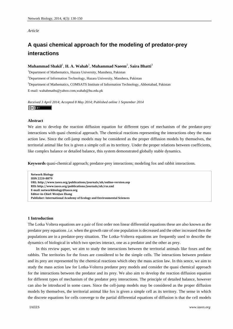
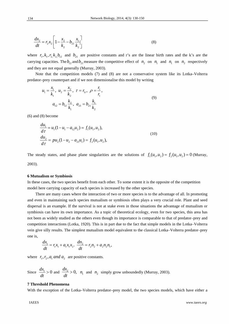
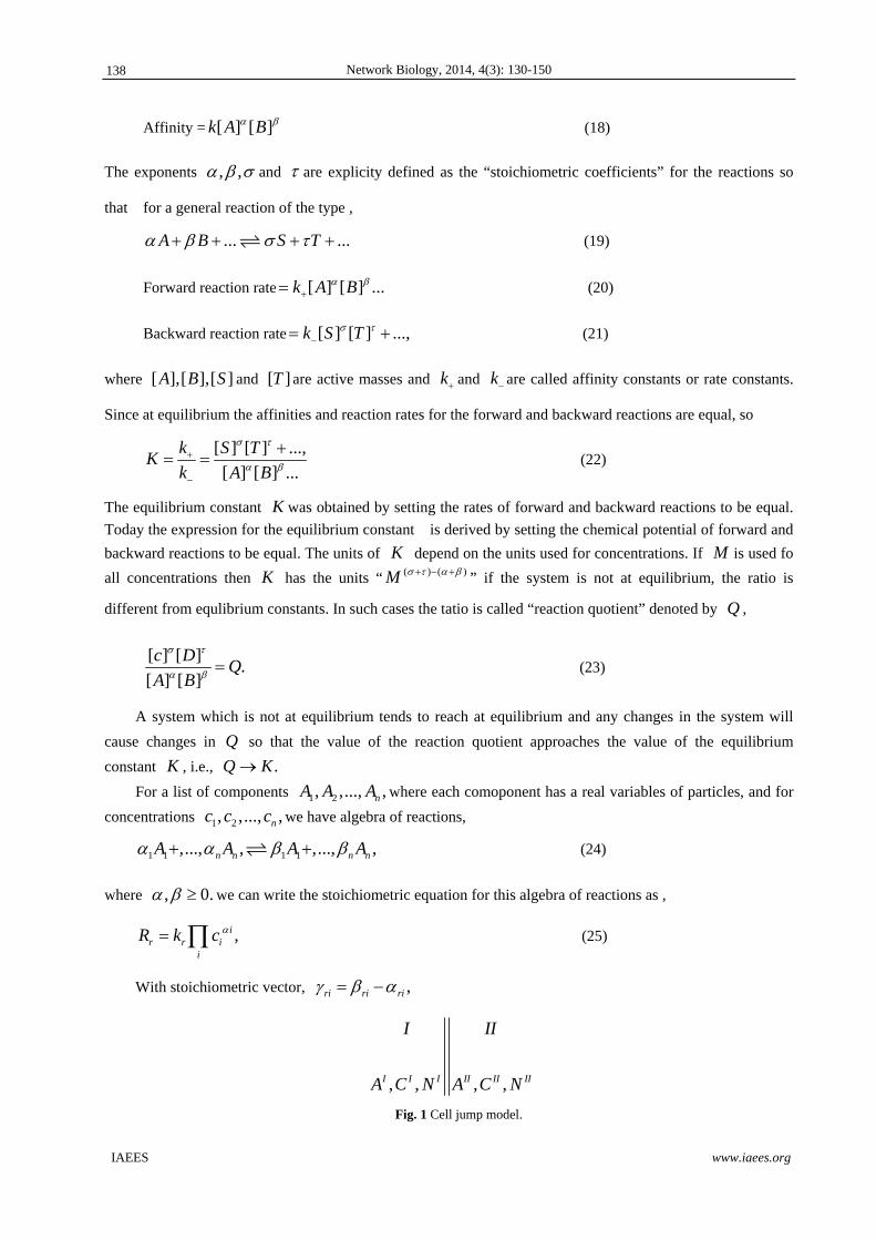
, , , ,I I I II II II
I II
A C N A C N
Fig. 1 Cell jump model.
138
Network Biology, 2014, 4(3): 130-150
IAEES www.iaees.org
11 A Simple Cell Jump Model
The standard form of reaction diffusion equation is,
( ) ,ii
cf c d c
t
(26)
where 0,id is diffusion coefficient and c should be literally small for very dialuted media (Gorban et al.,
2011).
The thermodynamic ideality is the general requirement of a system to apply the law of mass action.
Let us consider our space divided on cells, a system represented as a chain of cells each with homogeneous
composition and elementary acts of transfers on the boundary (for us there are only two cells). On each cell we
have some concentration for these processes. Let ,Ic is the vector concentration in the first cell I and ,IIc is
the vector of concentration in the second cell II .using the general secheme of the formal kinetics which is
considered to be complete if we work with list of macroscopic variables with balanced equations, a
mechanism of transformation (elementary process) and the functions of the rates of these elementary processes.
The mechanism of diffusion is defined as a list of elementary transitions between cells described by their
stoichiometric equation. Since diffusion is a sort of jumping reaction on the border, so for these jumps the
stoichiometric equation is written as,
,I I II II I I II IIri i ri i ri i ri i
i i i i
A A A A (27)
where r is the number of processes, , ,I IIri and ,I II
ri are the stoichiometric coefficients which indicate the
number of particles in cells involved in the process, where each process is is compared with the components
of the stoichiometric vector defined by ,I I Iri ri ri also there should be sysymmetry between these cells,
i.e. I IIi iA A , and diffusion coefficient id depends on the cell. Each elementary process is characterized by
an intensive quantity, termed as velocity function ( , )I IIr c c , (the number of elementary acts in a unit time
per unit surface of the cell). In the absence of convection and any chemical transformation the equation of
kinetics for the vector quantities, in isotropic and isothermal enviroment, is written as the equation of rate of
reaction,
,I II
r rr
dN dNS
dt dt (28)
where S is the area of the boundary between two cells. The i-flux density of a substance through a unit
surface of section is,
( , ) ( , ).I IIri ri rJ I II c c (29)
As a result of elementary acts of diffusion (27), the density of the total flux of the i-substance will be,
( , ) ,i ri ri rr
J J I II (30)
And the velocity function in the form of mass action law can be written as,
( , ) ( ) ( ) ,I IIri riI II I II
r i ii
c c k c c (31)
where 0rk is the rate constant depending upon the kinetic factors of the investigated system and its
139
Network Biology, 2014, 4(3): 130-150
IAEES www.iaees.org
thermodynamic properties. It is necessary to fulfil the no advection condition:
( , ) 0,r rr
c c (32)
which means the absence of flux at ,I IIc c in a homogeneous composition enviroment. Introducing flux
riJ as the first approximation of the Taylor series expansion in Subject to the condition (0.2.47),
( , )
. .
( )
I IIr
ri ri jIIj j I II
c cJ c
cc c c x
(33)
This expression represents the transition from flux density between the cells to the vector of the flux density. It
should be noted that model will work well, especially in the selection of the suitable relationship between
size of unit cell and diffusion zone (Gorban et al., 2011).
Gorban et al. (2011), Kuttler (2011), and Murray (2003) discussed a few diffusion reactions mechanisms
for cell jump models and determined their reactions rates, vectors of total flux density, and their diffusion
equations by using the law of mass action along with principle of detailed balance. Some of the mechanisms
are presented here.
12 Models of Non Linear Diffusion
The simplest mechanism of diffusion between any two cells is the process of jumping from one cell to another.
This type of mutually inverted and mutually inverse process can be written as (Gorban et al., 2011),
I II
II I
A A
A A
(34)
12.1 Mechanism of sharing place
The simplest mechanism of diffusion with interaction of n different substances of a multi component system is
given by stoichiometric equation of the form (Gorban et al., 2011):
I II I IIi j j i
II I I IIi j i j
A A A A
A A A A
(35)
12.2 Diffusion of mechanisms of attraction and repulsion
The diffusion mechanisms leading to the inhomogeneous structures can be described by the multi solution
immersed into the external conditions under which non linear mechanisms are possible with the stoichiometric
equations, describing the mechanism of attraction (Gorban et al., 2011):
Repulsion:
2
2
I I II
II I II
A A A
A A A
(36)
Attraction:
2
2
I II I
I II II
A A A
A A A
(37)
140
Network Biology, 2014, 4(3): 130-150
IAEES www.iaees.org
12.3 Autocatalysis mechanisms
A process where a chemical is involved in its own production is called autocatalysis. Feedbacks controls exist
into many biological systems. One must be familiar with how to model them because they have enormous
importance. In 1978, Tyson and Othmer introduced the dynamics of metabolic feedback control systems and a
theoretical models review. A process when the product of one step in a reaction sequence has an effect on
other reaction steps in the sequence. The effect is generally nonlinear and may be to activate or inhibit these
reactions. A very simple pedagogical example is,
1
2
2 ,k
kA Y Y (38)
where a molecule of Y combines with one of A to form two molecules of Y (Murray, 2003).
13 Foxes and Rabbits Interaction- A Non-Linear System
The humans are and they make open systems. Open systems interactions with the other open systems in an
immeasurable set of connections of open systems. Open systems become accustomed to these connections such
that their behaviour is non linear in general. It is difficult to predict the behavior of our artificial systems when
they are introduced into some operational atmosphere.
It is a constant battle among the animals on a daily basis to survive. They have to find their food and avoid
becoming a food. These species can be divide up on the basis that how they get their food, if they provide it
they are producers (prey), if they need to find it they are consumers (predator) and if they breakdown dead
material they are decomposers.
This correlation between predator and prey intertwines into a complex food chain. In the ecosystem there
are various species and every one play a significant role in maintaining populations near the carrying capacity
and in keeping the system in balance. In the ecosystems Predator and prey assist them through particular
adaptations to compete for food resources. Predator and prey populations are directly related and they cannot
survive without each other. Here this relationship is illustrated by using foxes and rabbits.
In artificial world and in the social systems non-linear behaviors are the order of the day. Rabbits and foxes
share some behaviors but vary in others and their interaction is non-linear in nature.
The rabbits are proverbially very good in reproduction. In case when more rabbits are there, the more foxes
will prey on them, so that the number of foxes will increase, when more foxes will predate a lot such that the
number of rabbits start to decrease, swiftly it follows by falling fox numbers as there are a small amount of
rabbits to sustain them therefore it is observed that the populations of rabbits and foxes are locked together in an
interactive population 'dance.' This system is non-linear in its behavior. In mathematics non-linear simultaneous
equations are used to represent these interactions for which there exist an infinite number of solutions.
Between the fox and rabbit populations here is a complicated and natural predator-prey relationship, since
rabbits thrive in the absence of foxes and foxes thrive in the presence of rabbits. Foxes like to occupy a
combination of forest and open fields. Foxes usually define their territory zones and use the transition zone or
"edge" between these habitats as hunting areas. Foxes do not interfere in the defined areas of each others.
13.1 Predator prey interactions
In this idealized ecological system, two populations are considered of which one may be hunted by the second.
Each prey gives rise to a constant number of off-spring preys each year.
A constant proportion of the prey population is hunted by each predator each year.
Predator reproduction is directly proportional to the constant proportion of the prey population hunted by
each predator.
141
IAEES
A co
If R is t
conventio
dR
ddF
d
The
to describ
other is i
Her
, ,A B C
A -
B -
C -
D -
Phy
evolution
dependin
the popu
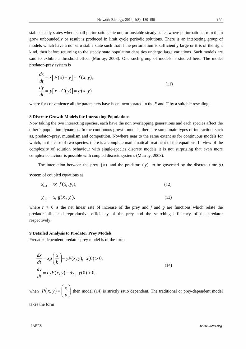
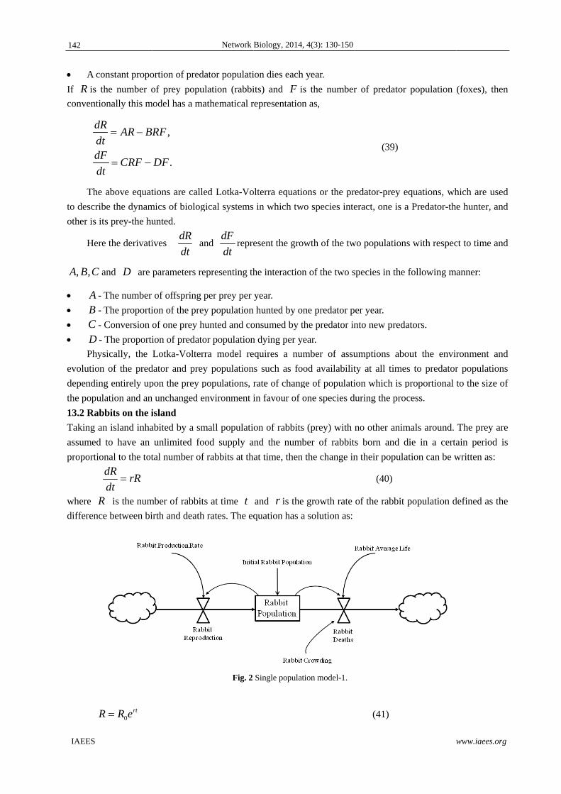
13.2 Rab
Taking a
assumed
proportio
where Rdifferenc
R
onstant propo
the number o
onally this m
RAR BR
dtF
CRFdt
e above equat
be the dynam
ts prey-the hu
re the derivati
and D are
The number
The proporti
Conversion
- The proporti
ysically, the
n of the pred
ng entirely up
lation and an
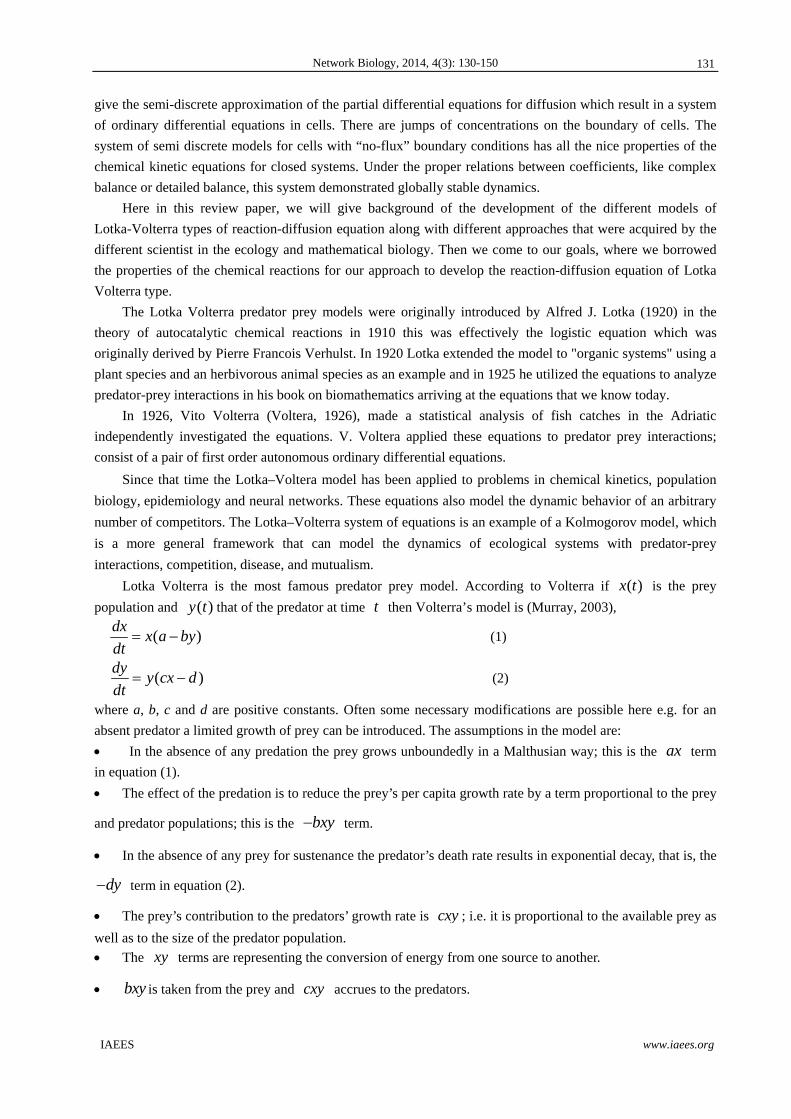
bbits on the i
an island inha
to have an
onal to the tot
dRrR
dt
R is the num
ce between bi
0rtR R e
ortion of pred
of prey popu
model has a ma
,
.
RF
DF
tions are call
mics of biolog
unted.
ives dR
dt a
parameters re
of offspring
ion of the pre
of one prey h
ion of predato
Lotka-Volter
dator and prey
pon the prey p
n unchanged e
island
abited by a sm
unlimited fo
tal number of
mber of rabbit
irth and death
Network
dator populati
ulation (rabbi
athematical r
led Lotka-Vo
gical systems
and dF
dtrepre
epresenting th
per prey per
ey population
hunted and co
or population
rra model re
y population
populations, r
environment i
mall populati
ood supply a
f rabbits at th
ts at time th rates. The eq
Fig. 2
Biology, 2014,
ion dies each
its) and F is
representation
olterra equatio
in which two
esent the grow
he interaction
year.
hunted by on
onsumed by th
n dying per ye
equires a num
ns such as foo
rate of chang
in favour of o
on of rabbits
and the numb
at time, then
and r is the
quation has a
Single populat
4(3): 130-150
year.
s the number
n as,
ons or the pre
o species inte
wth of the tw
n of the two s
ne predator p
he predator in
ear.
mber of assu
od availabilit
ge of populati
one species du
(prey) with n
ber of rabbits
the change in
growth rate
a solution as:
ion model-1.
r of predator
(39)
edator-prey e
eract, one is a
wo population
species in the
er year.
nto new preda
umptions abo
ty at all time
ion which is p
uring the pro
no other anim
s born and d
n their popula
(40)
of the rabbit
(41)
w
r population
equations, wh
a Predator-th
ns with respec
following m
ators.
out the envir
es to predator
proportional
ocess.
mals around.
die in a certa
ation can be w
population d
www.iaees.org
(foxes), then
hich are used
e hunter, and
ct to time and
anner:
ronment and
r populations
to the size of
The prey are
ain period is
written as:
defined as the
n
d
d
d
d
s
f
e
s
e
142
Network Biology, 2014, 4(3): 130-150
IAEES www.iaees.org
where 0R is the initial population of the rabbits (prey) at time 0t . This model is also called exponential
growth model due exponential factor involved. The exponential growth rate will be positive if births are more
than deaths and negative if deaths are dominant.
The exponential model is not very realistic because with a negative exponential growth rate, there will not
be any life left on the island. On the other hand, if the growth rate is positive, the rabbits will cover the entire
island with enough time. This will not happen actually because rabbits will run out of space and food due to
maximum carrying capacity of island. This kind of problem was handled through the law of population growth
derived by Alfred J. Lotka in 1925 by adding the concept of carrying capacity K to the exponential model.
This model is called logistic model formalized by the differential equation:
1dx x
rxdt k
(42)
Clearly when ,R K and R k the equation (42) is close to the equation (40) and rabbit population
stops growing. If ,R K then there will be a crowding of rabbit population on the island and from equation
(42) a negative sign will reduce the population growth to a manageable level. The behaviour of the model can
be predicted through the growth rate r .
13.3 Fox as a predator
In the presence of hundreds of different animals on the island, the modeling of the interaction among these
animals is not an easy task. However, the interaction between two species is possible taking one as a prey and
the other as a predator. The same single population growth model can be used for predators (foxes), if prey
(rabbits) is considered as an unlimited food supply to foxes. But Foxes are territorial animals, and in general
each fox claims its own territory by marking their territories with signals that other foxes will recognize e. g.,
by leaving their droppings in prominent positions. They pair up only in winter. So it will be difficult for the
foxes to cover the whole island without defining their own territories.
In order to describe the interaction between a predators (foxes) and its prey (rabbits), introduce a small
number of fox population on the island with rabbits having unlimited food supply and following the equation
(42). If R represents the rabbit’s population and F is the fox’s population, then population rates for each
species will be affected and described by the following equations as:
,
.
dRaR bRF
dtdF
cRF dFdt
(43)
where , ,a b c and d are parameters as defined for predator (fox) and its prey (rabbits). The additional terms
will now be defined as:
bRF Rabbits hunted by the foxes, reducing the rabbit population
cRF Fox population growth by eating the rabbits
Since some of the rabbits will be hunted by the foxes (as a food), so the birth rate r is not the only factor
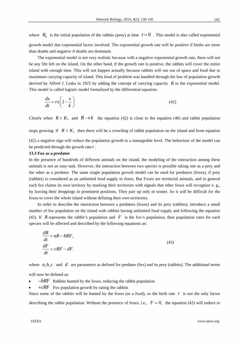
describing the rabbit population. Without the presence of foxes, i.e., 0,F the equation (43) will reduce to
143
IAEES
a simple
On
d
Which m
populatio
with the
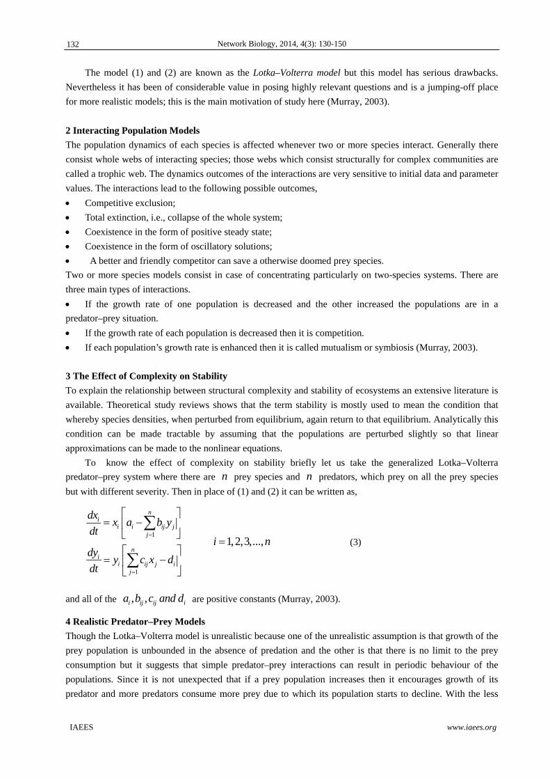
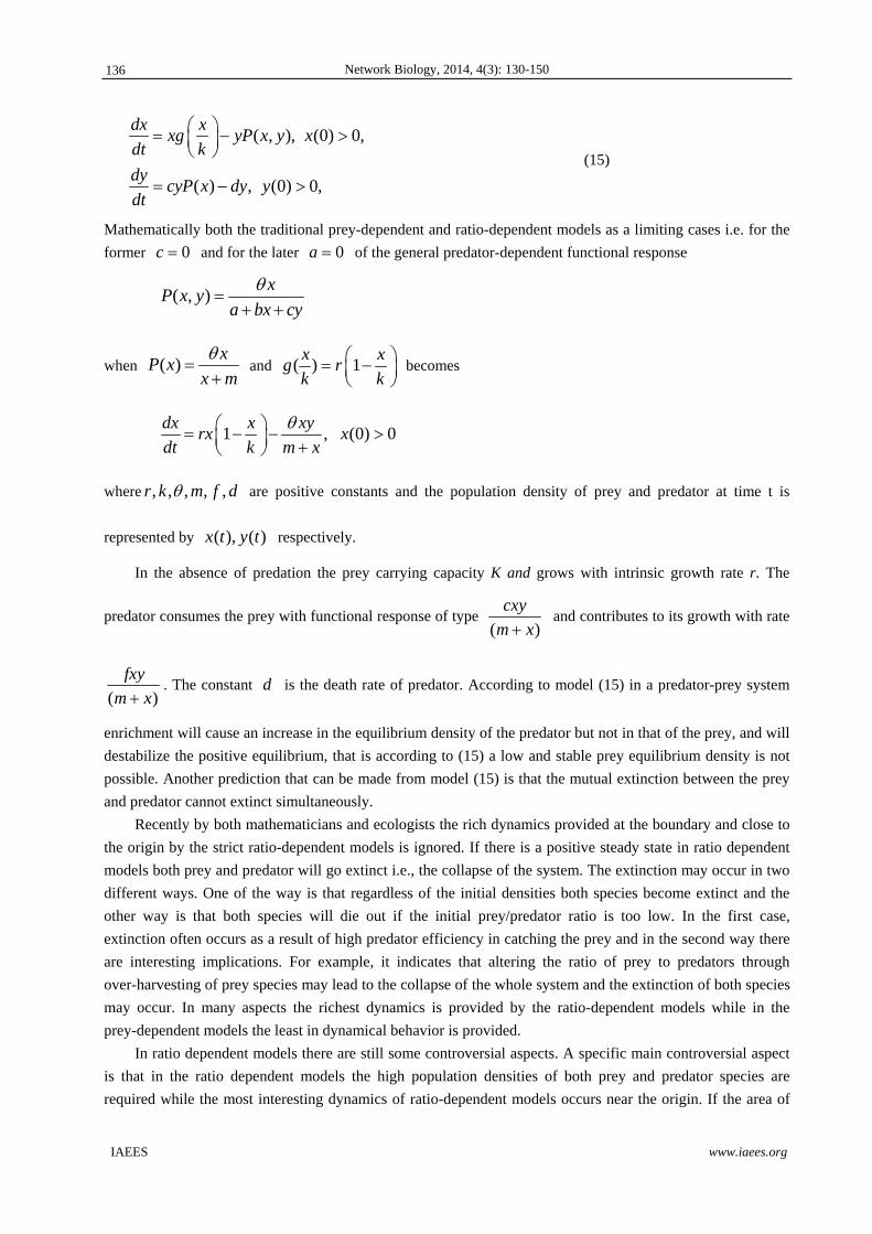
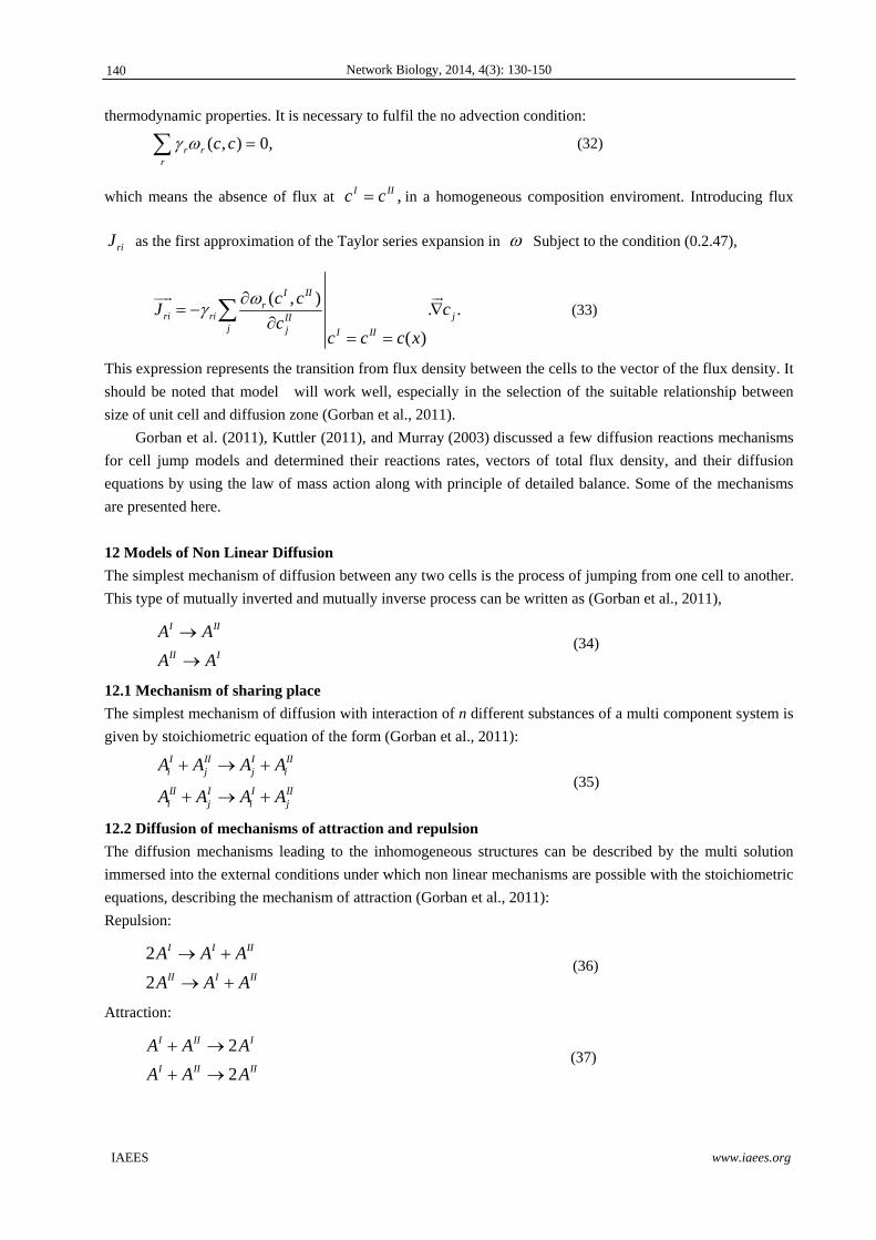
13.4 Bas
Let us su
with hom
territorie
Let IFthe first tvector of
In a
situation
1.
suppose
rabbit’s p
populatio
F
2.
n be t
combinat
(mF
exponential m
the other han
dFdF
dt
means foxes w
on will begin
increase in ra
sic reactions
uppose that o
mogeneous co
s). On each t
(fox/ foxes in
territory I andf concentratio
any territory w
;
Whe
that r is the
population w
on will increa
( )n R F
Now
the number o
tion of both
) ( ) (m fF
model (40).
nd, without fo
will die in tu
n to increase i
abbit populati
of foxes and
our space is d
omposition a
territory we h
n first territor
d IIF (fox/ fon in the seco
when foxes an
en in any ter
e number of r
will start to d
ase again; in t
( ) ,n r R
w in the case o
of foxes whic
( )m fF , this
( )( ) f mn F
Network
ood supply (R
urn if they do
in the absenc
ion, and this c
d rabbits
divided on tw
and elementar
have some co
ry) and IR (
foxes in seconond territory I
nd rabbits both
rritory a fox
rabbits which
decrease. Th
this case the p
r n
of foxes, whe
ch born as the
circle repeats
Biology, 2014,
Fig. 3 Mode
0)R to fo
o not get enou
ce of prey. Th
cycle will con
wo territories,
ry acts of tra
oncentrations
(rabbit/ rabbi
nd territory) II.
h are present,
( )F and to
h fox (F) prey
e rabbits are
possible mech
en two foxes,
e result of tha
s itself; in thi
4(3): 130-150
el structure.
oxes, the equa
ugh food for
he population
ntinue.
a system rep
ansfers on the
(number of
its in first ter
and IIR (ra
, the following
otal n numbe
y in that terri
e proverbially
hanism will b
a male fox F
at interaction
s case the po
ation (43) wil
(44)
their surviva
ns of foxes w
presented as a
e boundary (
foxes and rab
rritory) is the
abbit/ rabbits
g basic mech
er of rabbits
itory. When f
y very good
be,
(45)
( )mF and a fem
n, they all c
ssible mechan
(46)
w
ll reduce to:
al. In this cas
will again star
a chain of ter
for us there
bbits) for the
vector conce
in second ter
anisms are po
s ( )R are pr
fox will prey
in reproduc
male fox ( fF
an be males,
nism will be,
www.iaees.org
se, the rabbit
rts increasing
rritories each
are only two
se processes.
entration in
rritory) is the
ossible in that
resent, let us
y rabbits ( )R ,
ction so their
)f interact, let
females or a
,
t
g
h
o
.
n
e
t
s
,
r
t
a
144
Network Biology, 2014, 4(3): 130-150
IAEES www.iaees.org
3. Now in the case of rabbits, when two rabbits, one male ( )mR and the other female rabbit
( )fR interact, let n be the number of rabbits which born as the result of that interaction, they can be males,
females or a combination of both sexes ( )m fR , this circle repeats itself; in this case the possible mechanism
will be,
( ) ( ) ( )( )m f m fR R n R (47)
13.5 Mechanism of circulation
The simplest mechanism of circulation between any two foxes or rabbits is the process of moving one fox or
rabbit from area defined for it, to the area defined for another fox or rabbit and vise versa. This type of mutually
inverted and mutually inverse processes for the case of foxes can be written as,
I II
II I
F F
F F
(48)
This mechanism for the case of rabbits will be written as,
I II
II I
R R
R R
(49)
As it is stated in the early lines that foxes are territorial and stay in their own territorial zones, the above
mechanism may not be possible in practical in the case of foxes, but rabbits move freely in nature without any
restrictions so this mechanism may or may not be possible in that case.
13.6 Mechanism of sharing place
1. The mechanism of sharing place with interaction of n different foxes or rabbits i.e. when a fox IiF is in
territory one and another fox IIjF is in territory two and then fox I
iF moves from territory one to territory two
and vise versa, in a multi component system is given by stoichiometric equations of the form:
I II I IIi j j i
II I I IIi j i j
F F F F
F F F F
(50)
Practically in the case of foxes the above mechanism seems to be almost impossible because foxes usually define
their territory zones and use the transition zone or "edge" between these habitats as hunting areas. Foxes do not
interfere in the defined areas of each other’s and foxes fight other foxes if they find them in their territory.
2. In the case of rabbits it may or may not be possible because rabbit’s movement is free naturally without any
restrictions. In that case the possible mechanisms will be,
I II I IIi j j iR R R R (51)
II I I IIi j i jR R R R (52)
3. Now in the case of mix situation i.e. by taking foxes and rabbits case together,
I II I I Ii j i j iF R F R F (53)
145
Network Biology, 2014, 4(3): 130-150
IAEES www.iaees.org
II I II II IIi j i j iF R F R F (54)
As the foxes are territorial while the rabbits move freely, in the above mechanism (53) it is described that when a
fox is in territory one and a rabbit is in territory two, if rabbit move from territory two to territory one, the fox in
that area will prey that rabbit and a similar case happens in mechanism (54) for second territory.
13.7 Mechanism of attraction and repulsion
1. Foxes are solitary and necessitate quite huge hunting areas. A fox constantly patrols its territory looking
for food, using its urine to mark places it has completed searching. Foxes are territorial and fight other foxes
that they find on their territory. Because they wander over such a wide area, foxes maintain several burrows
and dens across their territory. The possible mechanisms of attraction and repulsion for the foxes and rabbits
can be;
Repulsion:
2
2
I I II
II I II
F F F
F F F
(55)
Attraction:
2
2
I II I
I II II
F F F
F F F
(56)
Both the mechanisms of attraction are unnatural in the case of foxes because foxes are territorial and fight other
foxes that they find on their territory so two or more foxes cannot stay in the same territory thus we will have
to move towards mechanisms of repulsion consequently there will be no attraction in the case of foxes.
2. Now taking the mechanisms of attraction and repulsion for the case of rabbits the following mechanisms
are possible,
Attraction:
2
2
I II I
I II II
R R R
R R R
(57)
Repulsion:
2
2
I I II
II I II
R R R
R R R
(58)
In this case the above stated both the mechanisms of attraction and repulsion may or may not be possible because
rabbits move freely in nature without any restrictions. If two rabbits are in two different territories and they both
move in the same territory then it is described by mechanisms of attraction and if two rabbits are in the same
territory and one of them leaves that territory and moves to another territory in that case, it is described by
mechanisms of repulsion.
3. Now for the mix situation i.e. when in any territory the mechanisms of attraction and repulsion are
considered for both, the foxes and the rabbits at a time, the following mechanisms for attraction and repulsion are
possible,
Attraction:
I I I
II II II
R F F
R F F
(59)
146
Network Biology, 2014, 4(3): 130-150
IAEES www.iaees.org
In attraction mechanism when both the rabbit and the fox are in the same territory, then fox will prey the rabbit
and the result will be the fox.
Repulsion:
I I I II
II II II I
R F F R
R F F R
(60)
In repulsion mechanism when both the rabbit and the fox will be in the same territory then it is possible that a
rabbit may change its territory but fox does not do so because foxes are territorial. When rabbit in the first
territory will change its territory then the fox of that territory will not be in a position to prey that rabbit so it will
survive that fox but fox present in that territory will be in a position to prey that rabbit and vise versa.
13.8 Pair wise interaction
In pair wise interaction the following mechanisms are possible because foxes are territorial while rabbits move
freely in nature and rabbits change their territories regularly while foxes does not do so. In this situation the
possible mechanisms will be;
( ) ( ) ( ) ( )I I II II II I I IIR F R F R F R F (61)
( ) ( ) ( )I I II II I I I IIR F R F R R F F (62)
( ) ( ) ( )I I II II I II II IIR F R F F R R F (63)
In the above mechanism (61) a rabbit and a fox are present in territory one and a similar situation is in the
territory two. In mechanism one, rabbit from territory one moves to territory two and vise versa. Other
possibilities are that both the rabbits move to territory one or both of them move to territory two. These
possibilities are described in mechanism (62) and (63) respectively.
13.9 Autocatalysis mechanisms
Autocatalysis is the procedure whereby a chemical is involved in its own production. In the following
mechanisms, in the case of foxes, when two foxes, a male fox ( )mF and a female fox ( )fF interact, let n be
the number of foxes which born as the result of that interaction, they all can be males, females or a
combination of both ( )m fF , this circle repeats itself; in this case the possible mechanism will be,
( ) ( ) ( )( )m f f mF F n F (64)
Now in the case of rabbits, when two rabbits, one male ( )mR and the other female rabbit ( )fR interact, let n
be the number of rabbits which born as the result of that interaction, they can be males, females or a
combination of both s ( )m fR , this circle repeats itself; in this case the possible mechanism will be,
( ) ( ) ( )( )m f m fR R n R (65)
14 The Observations
The sense in which the discrete equations for cells converge to the partial differential equations of diffusion is
that the cell models give the semi-discrete approximation of the partial differential equations for diffusion.
147
Network Biology, 2014, 4(3): 130-150
IAEES www.iaees.org
They result in a system of ordinary differential equations in cells. Such approximation appears often in finite
element methods and cells are discontinuous finite elements. There are jumps of concentrations on the
boundary of cells. The Taylor expansion of the right hand sides of the discrete system of ordinary differential
equations for cells produces the second order in the cell size approximation to the continuous diffusion
equation (the standard result for the central differences).
Significant difference from the classical finite elements is in construction of right hand sides of the
ordinary differential equations for concentrations in cells: there are flows in both directions: from cell 1 to cell
II and from cell II to cell I. These flows have a simple mass action law construction and the resulting diffusion
flow is the difference between them. The kinetic constants should be scaled with the cell size to keep kl d
(k is the kinetic constant, l is the cell size, d is the diffusion coefficient for the particular mechanism).
This is the approximation of the right hand sides. The approximation of solutions is a more difficult
problem and depends upon the properties of solutions of PDE. It seems a good hypothesis that for obtained
diffusion systems with convex Lyapunov functional and “no-flux” boundary conditions in bounded areas with
smooth boundaries the cell model gives the uniform approximation to the solution of the correspondent PDE.
The system of semi-discrete models for cells with “no-flux” boundary conditions has all the nice
properties of the chemical kinetic equations for closed systems. Under the proper relations between
coefficients, like complex balance or detailed balance, this system demonstrated globally stable dynamics. This
global stability property can help with the study of the related PDE.
Finally, the cell-jump models may be considered as the proper diffusion models by themselves, for the
finite physically reasonable cell size, without limit. This size may be quite large for the coarse-grained models
(it depends on the medium microstructure and on the smoothness of the concentration fields).
14.1 For mechanisms of circulation
For this mechanism,
I II
II I
I II
II I
F F
F F
R R
R R
It is stated in the early lines that the above stated mechanism is not possible in the case of foxes because the foxes
are territorial and does not change their territory while it may or may not be possible in the case of rabbits
because their movement is free naturally and if this mechanism occurs in their case, then the equation of
kinetics for the above mechanism the condition of absence of flux in a homogenous environment with the rate of
constant of direct and inverted processes as i i ik k k give the following form of the diffusion equation,
.ii i
ck c
t
14.2 For sharing place mechanism
Sharing place mechanism is also not possible in the case of foxes due to the fact that the foxes are territorial
and does not change their territory while it may or may not be possible in the case of rabbits because their
movement is free naturally and if this mechanism occurs in their case, then for the mechanisms of sharing
place the diffusion equations for the above mechanism using stoichiometric vectors ,ri
fluxes of the
substances iF and jF and the functions 1w and 2w for the first and second elementary process are
148
Network Biology, 2014, 4(3): 130-150
IAEES www.iaees.org
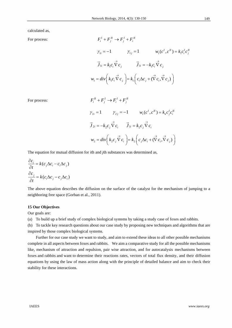
calculated as,
For process: I II I IIi j j iF F F F
1 1i 1 1j 1 1( , )I II I IIi jw c c k c c
1 1i i jJ k c c
1 1i i jJ k c c
1 1 1 ( , )i j i j i jw div k c c k c c c c
For process: II I I IIi j i jF F F F
2 1i 2 1j 1( , )I II I IIk j iw c c k c c
2 2i j iJ k c c
1 2i j iJ k c c
2 2 2 ( , )j i j i i jw div k c c k c c c c
The equation for mutual diffusion for ith and jth substances was determined as,
( )
( )
ij i i j
ji j j i
ck c c c c
tc
k c c c ct
The above equation describes the diffusion on the surface of the catalyst for the mechanism of jumping to a
neighboring free space (Gorban et al., 2011).
15 Our Objectives
Our goals are:
(a) To build up a brief study of complex biological systems by taking a study case of foxes and rabbits.
(b) To tackle key research questions about our case study by proposing new techniques and algorithms that are
inspired by those complex biological systems.
Further for our case study we want to study, and aim to extend these ideas to all other possible mechanisms
complete in all aspects between foxes and rabbits. We aim a comparative study for all the possible mechanisms
like, mechanism of attraction and repulsion, pair wise attraction, and for autocatalysis mechanisms between
foxes and rabbits and want to determine their reactions rates, vectors of total flux density, and their diffusion
equations by using the law of mass action along with the principle of detailed balance and aim to check their
stability for these interactions.
149
Network Biology, 2014, 4(3): 130-150
IAEES www.iaees.org
References
Abrams PA, Ginzburg LR. 2000. The nature of predation: prey dependent, ratio-dependent or neither? Tree, 15:
337-341
Alabdullatif M, Abdusalam HA, Fahmy ES. 2007. Adomian Decomposition Method for Nonlinear Reaction
Diffusion System of Lotka-Voltera Type. International Mathematical Forum, 2: 87-96
Berezovskaya F, Karev G, Arditi R. 2001. Parametric analysis of the ratio-dependent predator-prey model.
Journal of Mathematical Biology, 43(3): 221-246
Beretta E, Kuang Y. 1998. Global analyses in some delayed ratio-dependent predator-prey systems. Nonlinear
Analysis, 32: 381-408
Kuttler C. 2011. Reaction-Diffusion Equations with Applications. Sommersemester.
Douglas 1t. Boucher. 1982. The Ecology of Mutualism. 3: 315-347
Gorban AN, Sargsyan HP, Wahab HA. 2011. Quasichemical models of multicomponent nonlinear diffusion.
Mathematical Modelling of Natural Phenomena 6(5): 184-262. E-print: arXiv: 1012.2908
[cond-mat.mtrl-sci].
Hsu SB, Hwang TW, Kuang Y. 2001. Global analysis of the michaelis-menten type ratio-dependent
predator-prey system. Journal of Mathematical Biology, 42: 489-506
Hsu SB, Hwang TW, Kuang Y, 2001 Rich dynamics of a ratio-dependent one-prey two-predators model.
Journal of Mathematical Biology, 43: 377-396
Lotka AJ. 19200. Undamped oscillations derived from the law of mass action. Journal of American Chemical
Society, 42: 1595
Murray JD. 2003. Mathematical Biology I: An Introduction. Springer-Verlag
Voltera V. 1926.Variations and fluctuations of the number of the individuals in animal species living together.
In: Animal Ecology (Chapman RN, ed). McGraw-Hill, New York, USA
Wahab HA, Shakil M, Khan T, et al. 2013.A comparative study of a system of Lotka-Voltera type of PDEs
through perturbation methods, Computational Ecology and Software, 3(4): 110-125
150