occurrence of chaos and its possible control in a predator-prey model with density dependent...

June 11, 2010 14:13 WSPC/S0218-3390 129-JBS S0218339010003391

Journal of Biological Systems, Vol. 18, No. 2 (2010) 399–435c© World Scientific Publishing CompanyDOI: 10.1142/S0218339010003391

OCCURRENCE OF CHAOS AND ITS POSSIBLE CONTROLIN A PREDATOR-PREY MODEL WITH DENSITYDEPENDENT DISEASE-INDUCED MORTALITY

ON PREDATOR POPULATION

KRISHNA PADA DAS,∗,‡ SAMRAT CHATTERJEE†,§

and J. CHATTOPADHYAY∗,¶∗Agricultural and Ecological Research Unit

Indian Statistical Institute203, B. T. Road, Kolkata 700108, India

†Dipartimento di Matematica, Universita di Torinovia Carlo Alberto 10, 10123 Torino, Italia

‡krishna [email protected]§samrat [email protected]

¶[email protected]

Received 24 April 2009Accepted 1 March 2010

Eco-epidemiological models are now receiving much attention to the researchers. In thepresent article we re-visit the model of Holling-Tanner which is recently modified byHaque and Venturino1 with the introduction of disease in prey population. Densitydependent disease-induced predator mortality function is an important considerationof such systems. We extend the model of Haque and Venturino1 with density depen-dent disease-induced predator mortality function. The existence and local stability ofthe equilibrium points and the conditions for the permanence and impermanence of thesystem are worked out. The system shows different dynamical behaviour including chaosfor different values of the rate of infection. The model considered by Haque and Ven-turino1 also exhibits chaotic nature but they did not shed any light in this direction.Our analysis reveals that by controlling disease-induced mortality of predator due toingested infected prey may prevent the occurrence of chaos.

Keywords: Disease in Prey; Stability; Permanence; Impermanence; Chaos; LyapunovExponent.

1. Introduction

Eco-epidemiology is a relatively new branch in mathematical biology which consid-ers both the ecological and epidemiological issues simultaneously. The first break-through in modern mathematical ecology was done by Lotka and Volterra for apredator-prey competiting species. On the other hand, most models for the trans-mission of infectious diseases originated from the classic work of Kermack and

¶Corresponding author.

399

http://dx.doi.org/10.1142/S0218339010003391

June 11, 2010 14:13 WSPC/S0218-3390 129-JBS S0218339010003391

400 Das, Chatterjee & Chattopadhyay

Mc Kendrick.2 After these pioneering works, lots of research works have been doneboth in theoretical ecology and epidemiology. Anderson and May3 were probablythe first who merged the above two fields and formulated a predator-prey modelwhere prey species were infected by some disease. Many authors4,5 thus proposedand studied different predator-prey models in presence of disease. Chattopdhyayand Arino6 coined the name eco-epidemiology of such systems.

Successful invasion of a parasite into a host population depends crucially onother members of a host’s community such as predators.7 On the other hand,predation intensity can dramatically shape community structure and ecosystemproperties.8 Predation becomes particularly interesting in host-parasite systemsbecause predation itself can strongly alter population dynamics of hosts and par-asites.9–12 However, in many ecological studies of predator-prey systems with dis-ease, it is reported that the predators take a disproportionately high number ofparasite-infected prey.13–15 In this connection we like to mention that Holmes andBethel16 and Lafferty and Morris17 reviewed a number of the studies that havecontributed to the base of evidence in support of the hypothesis that parasitesmodify host behavior which results in increased susceptibility to predation. Holmesand Bethel16 examined predator-prey relationships and suggested two strategies bywhich parasites increased the likelihood of intermediate host predation including(1) reduction in host stamina as well as locomotor efficiency and (2) host disori-entation. For example, Brattey18 found that the acanthocephalan Acanthocephaluslucii causes changes in the pigmentation and behavior of aquatic isopods, whichmake them more susceptible to predation by perch, Perca fluviatilus. It is some-times observed that predators may have to pay a cost in terms of extra mortalityin the trade-off between the easier predation and the parasitized prey acquisitionbut the benefit is assumed to be greater than the cost. It is frequently observedin nature that consumption of infected prey becomes fatal to predator population.For example, the cats which predate on the song birds infected by salmonella canpick up the illness and die.a The case, consumption of infected prey contributenegative growth to predator population, was studied by Chattopadhyay et al.19

So the effect of consumption of infected prey on the growth of predator popula-tion is one of the vital issue on the research of eco-epidemiology. Chattopadhyayet al.20 considered a constant natural death as well as a disease-induced death dueto consumption of infected prey. In a realistic situation, disease-induced death ofpredator depends upon the consumption of infected prey. In this paper, we considerthe disease-induced mortality of predator in terms of density dependent responsefunction instead of constant disease-induced mortality.

The above descriptions clearly indicate that disease induced mortality plays animportant contribution in the dynamics of such eco-epidemiological systems. Asfar our knowledge goes, disease-induced mortality of predator in terms of density

ahttp://www.gov.nf.ca/agric/pubfact/salmonella.htm.

June 11, 2010 14:13 WSPC/S0218-3390 129-JBS S0218339010003391

Occurrence of Chaos and Its Possible Control in a Predator-Prey Model 401

dependent response function has not yet been considered in eco-epidemiologicalstudies. We like to re-visit Holling-Tanner model in this direction. Here we liketo mention that recently, Haque and Venturino1 studied the dynamics of Holling-Tanner model with introduction of disease in prey population. We have extended themodel of Haque and Venturino1 by introducing density dependent disease-inducedmortality in the predator population. The study of Haque and Venturino1 is notcomplete in the sense that their model exhibits chaotic dynamics, but unfortunatelythey did not pay attention in this direction.

In general chaotic nature is common of such systems. But unfortunately littleeffort has been made to study chaos in eco-epidemiological systems, though theliterature of chaos in ecological system is very rich. Recently Chatterjee et al.21

observed that rate of infection and the predation rate are two major factors thosegovern chaotic dynamics in eco-epidemiological system. On the other hand, birthrate22 and contact rate23 may be considered as possible parameters to elucidate theonset of chaotic behavior in an eco-epidemiological model. Therefore, the questionis — does increased infection rate produce unpredictable dynamics in our proposedsystem? To search for possible answers to this question, we have studied numericallyour proposed model for wide variation of force of infection. Our simulation resultsshow that our proposed system possesses different interesting dynamical behaviorstarting from chaos to limit cycle for increasing the rates of infection. Our simulationresults also show that limit cycle occurs in a reasonably large ranges of force ofinfection, whereas chaotic behavior has exhibited, intermixed with limit cycles, innarrow ranges of force of infection.

The paper is organized as follows. In Sec. 2, we outline the basic mathematicalmodel. We study the stability of the equilibrium points in Sec. 3 and the permanenceof the system in Sec. 4. We perform extensive numerical experiments in Sec. 5. Thearticle ends with a conclusion.

2. Model Formulation

The Holling-Tanner model for predator-prey interaction is given by

dN

dt= rN

(1 − N

K

)− mNPA+N

,

dP

dt= P

[θ

(1 − hP

N

)],

(1)

where N and P are the prey and predator populations. Prey population growlogistically with carrying capacity K and intrinsic growth rate r. The predatorconsumes the prey according to the Holling type-II functional response. Here, Arepresents the half-saturation constant and m is the searching efficiency constantfor the predator. The predator grows logistically with intrinsic growth rate θ andcarrying capacity proportional to the prey population size N . The parameter h

June 11, 2010 14:13 WSPC/S0218-3390 129-JBS S0218339010003391


is the number of prey required to support one predator at equilibrium when P

equals Nh .

The model system (1) is undefined at the origin. Recently there is a growinginterest among the researchers for this kind of models, specially after the famoustheory of ‘ratio-dependent’ proposed by Arditi and Ginzburg.24 In their paper theyused the ratio between the prey per predator in the functional response and termedit as the ratio-dependent functional response. After that, there were lots of articlesbeen published with this theory.25–32 Many researchers regarded ‘ratio-dependent’form to be more appropriate for defining predator-prey interactions where predationinvolves serious searching processes. Moreover this kind of models do not showthe two famous ecological paradoxes, viz., ‘paradox of enrichment’ and ‘biologicalcontrol paradox’. This further enhance the acceptance of the ratio-dependent theoryin the scientific community.

The main drawback in this kind of models is the discontinuity at the origin, dueto which it is not easy to study the dynamical behaviour of such system around theorigin. Thus such models have set up a challenging issue regarding their dynamicsnear the origin. Kuang and Beretta,33 Jost et al.,34 and Xiao and Ruan,35 observedthat the dynamics of such systems near the origin is more complicated since thevector field is not well defined at that point and cannot be linearized around thispoint. There exist numerous kinds of topological structures in the vicinity of theorigin (see, e.g., Berezovskaya et al.,36 and Xiao and Ruan35). This is the mainreason for ratio-dependent models possibly to have complicated rich dynamics.Kuang and Beretta33 proved that total extinction is also possible. Jost et al.34

proved that the origin can be a saddle-point or an attractor. Xiao and Ruan35

analyzed a situation where solutions reach the origin following a fixed direction.They observed that origin plays an important role in the global dynamics of suchsystems. Recently Arino et al.37 proposed a technique to study the behaviour of aratio-dependent model around the origin. They worked out the conditions for whichno trajectory can reach the origin following any fixed direction or spirally.

The model system (1) also has rich dynamics, some of which was explored byHaque and Venturino.1 In their article they extended the model (1) by introducingfollowing assumptions:

(A1): In presence of disease they divided the prey population into two classes,namely susceptible prey denoted by S(t), and infected prey denoted by I(t).They also considered that in absence of disease the prey population growslogistically with carrying capacity K ∈ R+ and intrinsic birth rate r ∈ R+.The susceptible prey was assumed to reproduce and contribute to its carryingcapacity. The infected prey do not grow, recover and reproduces, i.e. only sus-ceptible prey follows logistic growth. This consideration is based on the resultsof Hamilton et al.38 who showed that no infected individuals contribute to thereproduction. The experiment on dinoflagellate Noctiluca scintillans (miliaris)

June 11, 2010 14:13 WSPC/S0218-3390 129-JBS S0218339010003391


in the German Bight by Uhlig and Sahling39 indicated that the cells becomedamaged and they neither feed anymore or reproduce.

(A2): The transmission rate among the susceptible prey populations and theinfected prey populations was assumed to follow the simple law of mass actionλS(t)I(t) where λ is the transmission coefficient. The contact process is admit-tedly debatable. Some authors argue that the proportional mixing rate is moreappropriate than that of simple mass action law. In this context, Anderson40

plotted population sizes against R0 (basic reproduction number) for data setsregarding measles, pertussis, diphtheria and scarlet fever. Instead of showinga linear increase of R0 with population size, as predicted by mass action mod-els, R0 showed a weak non-linear increase with population size, R0 = βNv,(where N is total prey population) with estimates of v for different infectionsvarying between 0.03 and 0.07. Significance testing against the hypothesis thatin fact v = 0, or alternatively that v = 1, was not done but from the estima-tions the conclusion that v = 0, which is compatible with the proportionalmixing assumption seems more plausible. So it is obvious that comparativestudy with experimental data is essential for this situation to make any con-clusion. In the present study due to lack of data we simply assume mass actionlaw based partly on theoretical results and partly on greenwood experiments.Berthier et al.41 showed that mass action incidence assumption appears tobe more appropriate than proportional mixing to describe the dynamics ofdirect disease transmission. The data of Greenwood experiment suggest thatthere is no change of qualitative properties upon the contact process whetherit follows the law of mass action or it follows the proportinal mixing rate (DeJong et al.42).

(A3): Predators consumed both susceptible and infected prey with different maxi-mal predation rates denoted by m and n respectively. In nature it has beenobserved that m can be less or bigger than n depending on the type ofparasitism.43–45

With the above assumptions, the model (1) takes the following form:

dS

dt= rS

(1 − S

K

)− λIS − mPS

A+ S + I,

dI

dt= λSI − nPI

A+ S + I− γI,

dP

dt= P

[θ

(1 − hP

S + I

)],

(2)

where the old parameters retain the same meaning as in Eq. (1) and γ representsthe natural death rate of the infected prey.

Here we present the biological explanation of mass action disease transmis-sion. In homogeneous situation disease propagation depends on density of both

June 11, 2010 14:13 WSPC/S0218-3390 129-JBS S0218339010003391


susceptible host and infected individuals. In mass action (density dependent) trans-mission, susceptible hosts are assumed to contact other hosts throughout the wholeof their population at homogeneous mixing such that the number of these con-tacts rises in proportion to the size of the population. Disease models predictthat disease on its own cannot cause the complete extinction of a populationor species.46,47 The reason for this is that simple models of directly transmittedpathogens generally assume that disease transmission takes on a density-dependentform. Density-dependent disease transmission leads to host density thresholds belowwhich the disease cannot invade or persist,48,49 such that the disease is predicted todie out before the host population drops to extinction. Mass-action disease trans-mission function describes the instantaneous rate at which uninfected host indi-viduals become infected through contact with infected individuals. This representsthe net effect of two separate processes: (1) the rate of contact between infectedand uninfected individuals, and (2) the probability that a contact results in infec-tion. Density could potentially influence on these processes. For the first process,density dependent disease transmission assumes that the rate of contact increaseslinearly with the density of both uninfected and infected individuals. As the densityof infected individuals increases, each susceptible individual comes in contact withmore infected individuals per unit time.

Another important factor is half-saturation constant (A) which is involved infunctional responses. When total prey population S + I is scarce, the level of pre-dation is mainly limited by ability to capture or find the prey species, whereasat high density of prey population, the requirement to assimilate the prey speciesbecomes the limiting factor. Alternatively, a predator may become satiated andstop feeding. Here the parameter A, which is called half-saturation constant, is theprey population where predation rate attain 50% of its maximal predation rate.Sometimes it is useful to compare the capability of species to compete for preypopulation.50,51 The half-saturation constant determines how fast the predationrate approaches the maximal predation rate. Low values of A describe a rapidlyrising curve.

Predator growth equation:In the above model the growth equation of predator population is

dP

dt= P

[θ

(1 − hP

S + I

)].

In this equation there is no disease induced death rate term but consumptionof infected prey has a negative feedback on predator growth equation. It is wellknown that Avian diseases (such like Avian botulism (Clostridium botulinum typeC), Avian cholera (Pasteurella multocidia) and Avian salmonellosis (Salmonellatyphimurium) affect and kill waterfowl, shorebirds and water birds.52,53 It isobserved that the predation of infected prey causes mortality of predator, for exam-ple, since mid-August of 1996, a bacterial outbreak of Vibro vulnificus in the Salton

June 11, 2010 14:13 WSPC/S0218-3390 129-JBS S0218339010003391


sea among the Tilpia has led to massive deaths not only among the fish themselves,but also in the pelican population. Studies have indicated that the bacterial infec-tion contributes to low oxygen levels in the tissues of the infected fish. The shortageof oxygen causes the fish to seek oxygen from the sea’s surface and leads to a favor-able environment for botulism to grow in the tissues of the infected fish.20 Whenpelicans prey upon these vulnerable fishes, it is likely that they ingest the botulismtoxins that eventually contribute to the development of Avian botulism. Avianbotulism is a debilitating neurological disease which usually inflicts death upon itshost.54 So it clear that mortality of the pelicans depends on consumption of infectedfish.

The above description motivates us to modify the growth equation of preda-tor population. We include the density dependent disease-induced mortality dueto ingested infected prey. So the growth equation of predator population can bewritten as

dP

dt= P

[θ

(1 − hP

S + I

)]− ψnPI

A+ S + I.

Here total consumption of infected prey by predator population is nPIA+S+I and

mortality term of predator population due to ingested infected prey is ψnPIA+S+I ,

which is called density dependent disease-induced mortality on predator populationdue ingested infected prey because it depends on predated infected prey. ψ is themortality efficiency (generally it is called mortality rate) due to ingested infectedprey.

By introducing density dependent disease-induced mortality of predator due toingested infected prey the system (2) eventually becomes

dS

dt= rS

(1 − S

K

)− λIS − mPS

A+ S + I= F1(S, I, P ),

dI

dt= λSI − nPI

A+ S + I− γI = F2(S, I, P ),

dP

dt= P

[θ

(1 − hP

S + I

)]− ψnPI

A+ S + I= F3(S, I, P ).

(3)

System (3) has to be analyzed with the following initial conditions:

S(0) > 0, I(0) > 0, P (0) > 0.

3. Equilibria and Their Local Stability

3.1. Equilibria and their existence

The system has five equilibrium points. The trivial equilibrium point E0(0, 0, 0)and the axial equilibrium point E1(K, 0, 0) exist for all parametric values.

June 11, 2010 14:13 WSPC/S0218-3390 129-JBS S0218339010003391


Disease-free equilibrium point is E2(S, 0, P ), where

S =(rKh−mK − rAh) +

√(rKh−mK − rAh)2 + 4h2AK

2rh, P =

S

h.

The existence condition of disease-free equilibrium point E2 is

rKh > mK + rAh.

The endemic equilibrium point is E3(S, I, 0), where S = γλ , I = r(Kλ−γ)

Kλ2 Theexistence condition of planar equilibrium point E3 is Kλ > γ.

The interior equilibrium point is given by E∗(S∗, I∗, P ∗), where S∗ is the posi-tive root of the equation

Q1S3 +Q2S

2 +Q3S +Q4 = 0, (4)

where Q1, Q2, Q3 and Q4 are given in Appendix A.

I∗ =K(rn+mγ) − (rn+ λmK)S∗

λnK, and P ∗ =

S∗ + I∗

h

[1 − ψnI∗

θ(A+ S∗ + I∗)

].

The interior equilibrium point E∗ exists if the following conditions hold

K(rn+mγ) > (rn+ λmK)S∗,ψnI∗

θ(A+ S∗ + I∗)< 1. (5)

Remark 3.1. Equilibrium points E0(0, 0, 0), E1(K, 0, 0), E2(S, 0, P ), E3(S, I, 0)of the system (3) are same as those of the system (2). E∗(S∗, I∗, P ∗) andE∗(S∗, I∗, P ∗) are the interior equilibrium points of system (3) and system (2)respectively. Here S∗ is the positive root of the Eq. (4) with ψ = 0 and I∗ and P ∗

are obtained from (5) by substituting S∗ = S∗ and ψ = 0.

Remark 3.2. The Eq. (4) is a cubic equation and so there is a chance of multiplepositive roots. But, for the sake of simplicity, here we consider the case for whichonly one positive root exists. For example, let us choose the following hypotheticalset of parameter values r = 2.5,K = 1, A = 0.2,m = 1, n = 0.433, γ = 0.1, h =2.26, θ = 0.008, λ = 2.8 and ψ = 0.0. For these set of parameter values Eq. (4)becomes

− 0.36092S3 + 0.422819S2 − 0.140671S + 0.00950824 = 0. (6)

Equation (6) has three positive roots 0.0901307, 0.53368 and 0.54769. Substitutingthese values in the expression of I∗ and P ∗ we observe that there exists one positiveequilibrium point E∗(0.0901307, 0.68671, 0.343735).

If we include ψ = 0.004, Eq. (4) becomes

− 0.36092S3 + 0.415044S2 − 0.13486S + 0.00845957 = 0. (7)

June 11, 2010 14:13 WSPC/S0218-3390 129-JBS S0218339010003391


Equation (7) has one positive root 0.081903 and substituting this value in theexpression of I∗ and P ∗ we get one positive equilibrium point of system (3) asE∗(0.081903, 0.713058, 0.297175). Now we if put ψ = 0.03, we notice that interiorequilibrium point E∗(0.081903, 0.713058, 0.297175) converges to endemic equilib-rium point E3(0.0181381, 0.917254, 0).

We like to mention here that the system has admit multiple interior equilibriumpoints. And the system with those equilibrium points may give rise to some inter-esting dynamics both from analytical and biological point view. We leave this issuefor future studies.

Remark 3.3. It is interesting to note that if λ attain some critical value, sayλc = K(rn+mγ)−rnS∗

KS∗m , then the interior steady state E∗ approaches the disease-freesteady state E2. Thus we may conclude that by controlling the rate of infection,the system can be made disease-free.

The Jacobian matrix J of the system (3) at any arbitrary point (S, I, P ) isgiven by

J ≡

r(1 − 2S

K ) − λI − mP (A+I)(A+S+I)2 −λS + mPS

(A+S+I)2 − mSA+S+I

λI + nPI(A+S+I)2 λS − nP (A+S)

(A+S+I)2 − γ − nIA+S+I

hθP 2

(S+I)2 + ψnPI(A+S+I)2

hθP 2

(S+I)2 − ψnP (A+S)(A+S+I)2 θ(1 − 2hP

S+I ) − ψnIA+S+I

.

(8)

3.2. The continuity of model system and local stability

of E0(0, 0, 0)

From system (3) it is clear that it is not defined at (0, 0, 0). So, system (3) isredefined with

F1(0, 0, 0) = 0, F2(0, 0, 0) = 0, F3(0, 0, 0) = 0.

Due to the boundedness of the functional response we see that

lim(S,I,P )→(0,0,0)

F1(S, I, P ) = lim(S,I,P )→(0,0,0)

F21(S, I, P )

= lim(S,I,P )→(0,0,0)

F3(S, I, P ) = 0

Using the system (3), we conclude that the functions F1(S, I, P ), F2(S, I, P ),F3(S, I, P ) are continuous functions on +

3 = (S, I, P ) : S ≥ 0, I ≥ 0, P ≥ 0.55,56At the trivial equilibrium point E0, due to discontinuity, it is difficult to study

the stability of the system around the origin. To study the dynamic around theorigin, one could use the technique proposed by Arino et al.37 and worked out theconditions for the trajectories to reach the origin. The proof is similar to Arinoet al.37 and hence the study is omitted.

June 11, 2010 14:13 WSPC/S0218-3390 129-JBS S0218339010003391


3.3. Local stability of nontrivial equilibrium points and biological

significant of threshold parameter

Theorem 3.1. The axial equilibrium point E1 are always unstable. The disease-free equilibrium point E2 is locally stable if

R02 < 1 andmP

(A+ S)2< min

r

K+θhP

S2,r

K+

Pm

S(A+ S)

,

where R02 = λSnPA+S+γ

.

The endemic equilibrium point E3 is locally stable if R03 < 1 where, R03 =θψnI

A+S+I

.

See Appendix B for the proof.

3.3.1. Biological significance of threshold parameters

Here we will explain the biological significance of threshold parameters obtainedfrom local stability analysis o equilibrium point, each of which has clear and distinctbiological meaning.

We first define the disease basic reproduction number R02 given by

R02 =λS

nPA+S

+ γ,

which has important role in determining the stability of disease-free equilibriumpoint E2(S, 0, P ). Here λS is the infection rate of a new infective prey appearing in atotally susceptible prey population and nP

A+S+γ is the removal rate of infective prey

at E2. So, 1nPA+S+γ

is the duration of infectivity of an infective prey and consequently

R02 is the disease basic reproduction number of disease in the prey population.R02 < 1 implies disease will be eradicated in the prey population.

We also define ecological basic reproduction number R03 by

R03 =θψnI

A+S+I

,

which determines the local stability of endemic equilibrium point E3(S, I, 0). Here θis the intrinsic growth rate of predator population and ψnI

A+S+Iis the mortality rate

due to ingested infected prey at E3. So, 1ψnI

A+S+I

can interpreted as mean lifespan of

a predator. Subsequently R03 gives the mean number of newborn predators by apredator, which can be interpreted as the ecological basic reproduction number ofa predator at E3. R03 < 1 implies the predator will become extinct and this resultsin E3 being locally stable.

Here we have introduced ecology and disease basic reproduction numbers. So,we give the biological explanation of basic reproduction numbers in general way

June 11, 2010 14:13 WSPC/S0218-3390 129-JBS S0218339010003391


and we also explain ecology and disease basic reproduction number and their inter-relationship. Basic reproduction number can be defined as the expected number ofoffspring produced by individuals in its life period. Ecological basic reproductionnumber is interpreted as the mean number of newborn predators by a predator.We also note that this term, first formulated and explained by Pielou,57 is theaverage number of prey converted to predator biomass in a course of the preda-tor’s life span.4 The disease basic reproduction number is the expected number ofsecondary infections produced by a single infective individual in a completely sus-ceptible population during its entire infectious period. So both basic reproductionnumbers represent mean number of offspring: ecological basic reproduction numbergives newborn individuals which can not spread disease, and disease basic reproduc-tion number gives newborn individuals which can spread disease in the environment.Here R02 and R03 are ecological and disease basic reproduction number respectivelyand we analyze the community structure of our model system. R02 < 1 implies thatdisease in prey will be wiped out and R03 < 1 implies that predator populationgoes to extinction. So by these reproduction numbers we determine the persistenceor extinction of species in our model system. This has allowed us to categorize thecommunity composition of disease and predator. This threshold concept has beenused in previous studies of eco-epidemiological models.4,58,59

Remark 3.4. The introduction of density dependent disease-induced mortalitydue to ingested infected prey on predator population does not change the localstability of boundary equilibrium points E0, E1, E2 of the system (2). But thisinclusion has changed the local stability of endemic equilibrium point E3. Theendemic equilibrium E3 of the system (3) is stable under the following conditionR03 < 1.

Theorem 3.2. The interior point E∗(S∗, I∗, P ∗) for the system (3) is locallyasymptotically stable if the following conditions hold

f1(S∗, I∗, P ∗) = RS∗ + hθP ∗N∗ − (mS∗ + nI∗)P ∗A21 > 0,

f2(S∗, I∗, P ∗) = σ1σ2 − σ3 > 0,

f3(S∗, I∗, P ∗) = σ3 > 0,

(9)

where σi’s are given in the proof of the theorem.

See Appendix C for the proof.

Remark 3.5. The interior equilibrium point E∗(S∗, I∗, P ∗) of the system (2) islocally asymptotically stable if the following conditions are true:

f1(S∗, I∗, P ∗) = RS∗ + hθP ∗N∗ − (mS∗ + nI∗)P ∗A21 > 0,

f2(S∗, I∗, P ∗) = σ1σ2 − σ3 > 0,

f3(S∗, I∗, P ∗) = σ3 > 0.

June 11, 2010 14:13 WSPC/S0218-3390 129-JBS S0218339010003391


This can be easily obtained from the condition (9) by putting S∗ = S∗, I∗ = I∗,P ∗ = P ∗, N∗ = N∗ and ψ = 0. The density dependent disease-induced mortality ofpredator due to ingested infected prey may change the stability of E∗(S∗, I∗, P ∗).It is difficult to show analytically due to complexity of the expression and we willtake the help of numerical simulation.

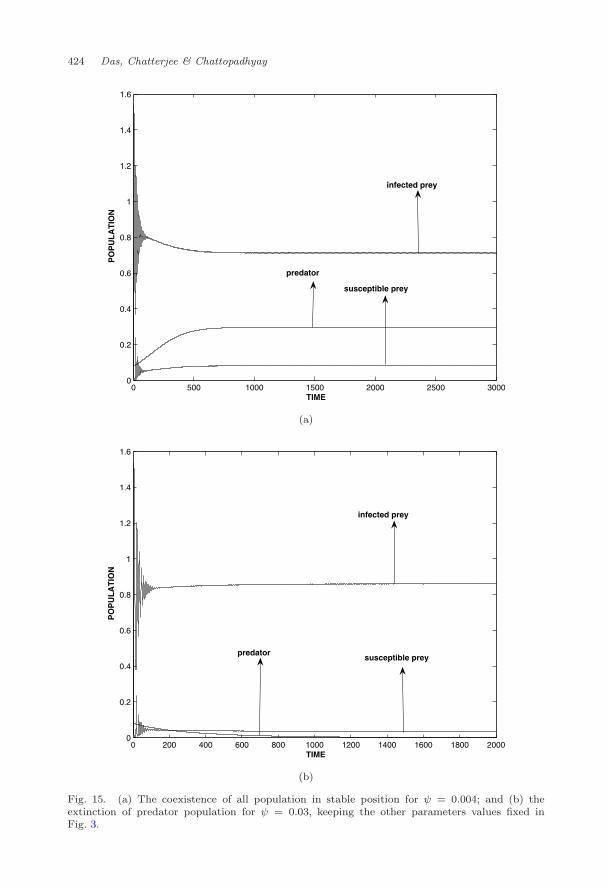
Example 3.1. Let us consider the following hypothetical set of parameter valuesr = 2.5,K = 1, A = 0.2,m = 1, n = 0.433, γ = 0.1, h = 2.26, θ = 0.008, λ =2.8 and ψ = 0.0. For these set of parameter values we have f1(S∗, I∗, P ∗) =0.1090, f2(S∗, I∗, P ∗) = 0.0362 and f3(S∗, I∗, P ∗) = 0.0105. So Routh-Hurwitzcriteria is satisfied and thus the system (2) is stable around the interior equilib-rium point E∗(0.0901307, 0.68671, 0.343735) (Fig. 3). Now if we include ψ = 0.004Routh-Hurwitz criteria for system (3) f1(S∗, I∗, P ∗) = 0.1102, f2(S∗, I∗, P ∗) =0.0359 and f3(S∗, I∗, P ∗) = 0.0097 are satisfied. So, the interior equilibrium pointE∗(0.081903, 0.713058, 0.297175) is locally asymptotically stable for system (3)(Fig. 15(a)).

If we increase the value of ψ from 0.004 to 0.03 the interior equilibrium pointE∗(0.081903, 0.713058, 0.297175) of system (3) converges to endemic equilibriumpoint E3(0.0181381, 0.917254, 0). This indicates that due to enhancement of densitydependent death parameter, the predator population eventually goes to extinctionand special consideration has to be given in such situation.

4. Permanence of the System (3)

From biological point of view, permanence of a system means the survival of allpopulations of the system in future time. Mathematically, permanence of a sys-tem means that strictly positive solutions do not have omega limits points on theboundary of the non negative cone.

Theorem 4.1. If the condition R03 > 1 is satisfied and further if there exists aperiodic solutions S = Φ(t), P = Ψ(t), in the S − P plane, then system (3) isuniformly persistent provided for the periodic solutions of period T,

η = −γ +1T

∫ T

0

(λΦ − nΨ

(A+ Φ)

)dt > 0. (10)

Proof. Let x be a point in the positive quadrant and o(x) be orbit through x andΩ be the omega limit set of the orbit through x. Note that Ω(x) is bounded.

We claim that E0 /∈ Ω(x). If E0 ∈ Ω(x) then by the Butler-McGehee lemmathere exists a point P in Ω(x)

⋂W s(E0) where W s(E0) denotes the stable manifold

of E0. Since o(P ) lies in Ω(x) and W s(E0) is the I axis, we conclude that o(P ) isunbounded, which is a contradiction.

Next E1 /∈ Ω(x), otherwise, since E1 is a saddle point (which follows fromJacobian matrix around E1), by the Butler-McGehee lemma there exists a point P

June 11, 2010 14:13 WSPC/S0218-3390 129-JBS S0218339010003391


in Ω(x)⋂W s(E1). Now W s(E1) is the S axis implies that an unbounded orbit lies

in Ω(x), which is a contradiction.Next we show that E3 /∈ Ω(x). If E3 ∈ Ω(x), the condition R03 > 1 implies

that E3 is a saddle point. W s(E3) is the S − I plane and hence the orbits in thisplane emanate from either E0 or E1 or an unbounded orbit lies in Ω(x), again acontradiction.

Lastly we show that no periodic orbit in the S−P plane or E2 ∈ Ω(x). Let theJacobian matrix J given in (8) at (Φ(t), 0,Ψ(t)) be denoted by J(Φ(t), 0,Ψ(t)).

Computing the fundamental matrix of the linear periodic system,

X ′ = J(t)X, X(0) = X0.

We find that its Floquet multiplier in the I direction is eηT . Then proceeding in ananalogous manner like Kumar and Freedman,60 we conclude that no periodic orbitlies on Ω(x). Thus, Ω(x) lies in the positive quadrant and system (3) is persistent.Finally, since only the closed orbits and the equilibria from the omega limit set ofthe solutions on the boundary of R3

+ and system (3) is dissipative. Now using atheorem of Butler et al.,61 we conclude that system (3) is uniformly persistent.

Remark 4.1. If the condition R03 > 1 and a finite number of periodic solutionsexist in S−P plane, the system (3) is uniformly persistent if corresponding to eachperiodic solution Floquet multiplier in the I is positive.

The proof is similar to the Theorem 4.1.In the Theorem 4.1 and Remark 4.1, we have shown the relation between the

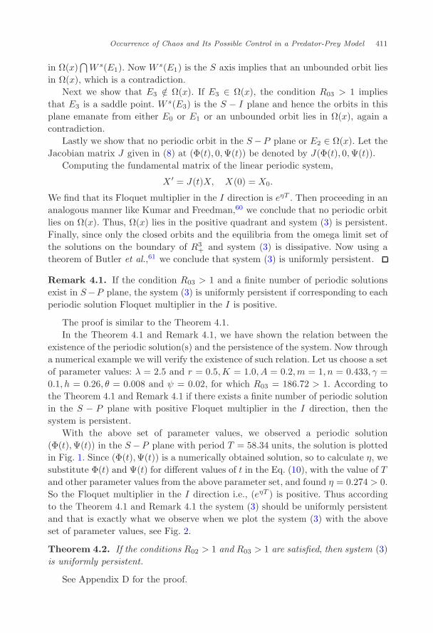
existence of the periodic solution(s) and the persistence of the system. Now througha numerical example we will verify the existence of such relation. Let us choose a setof parameter values: λ = 2.5 and r = 0.5,K = 1.0, A = 0.2,m = 1, n = 0.433, γ =0.1, h = 0.26, θ = 0.008 and ψ = 0.02, for which R03 = 186.72 > 1. According tothe Theorem 4.1 and Remark 4.1 if there exists a finite number of periodic solutionin the S − P plane with positive Floquet multiplier in the I direction, then thesystem is persistent.

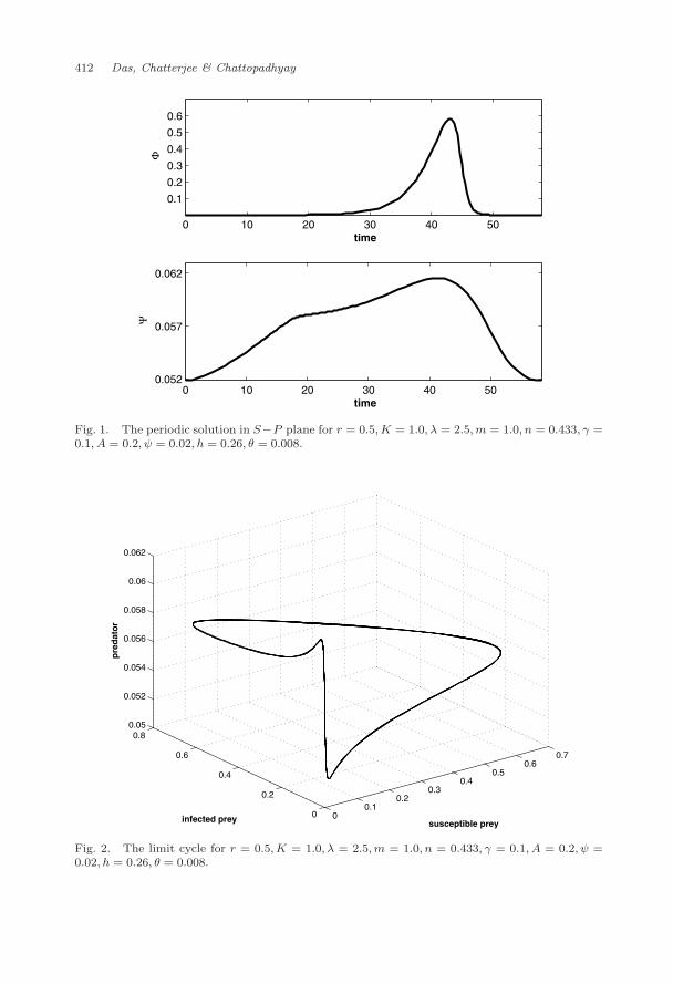
With the above set of parameter values, we observed a periodic solution(Φ(t),Ψ(t)) in the S−P plane with period T = 58.34 units, the solution is plottedin Fig. 1. Since (Φ(t),Ψ(t)) is a numerically obtained solution, so to calculate η, wesubstitute Φ(t) and Ψ(t) for different values of t in the Eq. (10), with the value of Tand other parameter values from the above parameter set, and found η = 0.274 > 0.So the Floquet multiplier in the I direction i.e., (eηT ) is positive. Thus accordingto the Theorem 4.1 and Remark 4.1 the system (3) should be uniformly persistentand that is exactly what we observe when we plot the system (3) with the aboveset of parameter values, see Fig. 2.

Theorem 4.2. If the conditions R02 > 1 and R03 > 1 are satisfied, then system (3)is uniformly persistent.

See Appendix D for the proof.

June 11, 2010 14:13 WSPC/S0218-3390 129-JBS S0218339010003391


0 10 20 30 40 50

0.1

0.2

0.3

0.4

0.5

0.6

time

Φ

0 10 20 30 40 500.052

0.057

0.062

time

Ψ

Fig. 1. The periodic solution in S−P plane for r = 0.5,K = 1.0, λ = 2.5,m = 1.0, n = 0.433, γ =0.1, A = 0.2, ψ = 0.02, h = 0.26, θ = 0.008.

00.1

0.20.3

0.40.5

0.60.7

0

0.2

0.4

0.6

0.80.05

0.052

0.054

0.056

0.058

0.06

0.062

susceptible prey infected prey

pre

dat

or

Fig. 2. The limit cycle for r = 0.5,K = 1.0, λ = 2.5,m = 1.0, n = 0.433, γ = 0.1, A = 0.2, ψ =0.02, h = 0.26, θ = 0.008.

June 11, 2010 14:13 WSPC/S0218-3390 129-JBS S0218339010003391


Next we shall find the condition for the impermanence of the system (3). Beforeobtaining the conditions for impermanence of system (3), we briefly define theimpermanence of a system. Let x = (x1, x2, x3) be the population vector, let D =x : x1, x2, x3 > 0, and ∂D is the boundary of D. ρ(., .) is the distance in R3

+.Let us consider the system of equations are

x = xifi(x), i = 1, 2, 3,

where fi:R3+ → R and fi ∈ C1.

The semi-orbit γ+ is defined by the set x(t): t > 0 where x(t) is the solutionwith initial value x(0) = x0.

The above system is said to be impermanent if and only if there is an x ∈ D

such that limt→∞ ρ(x(t), ∂D) = 0.62 Thus a community is impermanent if there isat least one semi-orbit which tends to the boundary.

Theorem 4.3. If the condition R03 < 1 holds, then the system (3) is impermanent.

Proof. The given condition R03 < 1 implies that E3 is a stable equilibrium pointon the boundary. Hence, there exists at least one orbit in the interior that convergesto the boundary63 and consequently the system (3) is impermanent.62

Remark 4.2. If there exists a finite number of periodic solutions S = Φr(t), P =Ψr(t), r = 1, 2, . . . , n, in the S − P plane, then system (2) is uniformly persistentprovided for each periodic solutions of period T ,

ηr = −γ +1T

∫ T

0

(λΦr − nΨr

(A+ Φr)

)dt > 0,

r = 1, 2, . . . , n.If the conditions R02 > 1 is satisfied then system (2) is uniformly persistent.

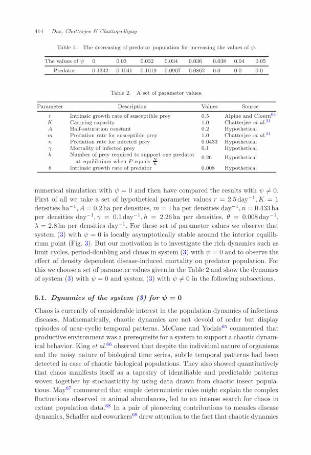
If we assume that the system (2) is permanent then we can say from Theo-rems 4.1–4.3 that system (3) is permanent or impermanent with respect to thesystem (2) according as the condition R03 > 1 or R03 < 1. As disease-inducedparameter ψ has negative impact on predator population, the proposed systemtends to impermanency for increasing the values of ψ. Biologically these results arein accordance with the Avian diseases that is described in conclusion part. It isinteresting to note that the predator population decreases and eventually goes toextinction for higher values of ψ (Table 1). We have used the hypothetical set ofparameter values given in Table 2 (which is used for entire numerical experimentsof the system).

5. Numerical Experiments

In this section, we have performed extensive numerical experiment to study the roleof disease-induced mortality of the predator in system (3). We have first performed

June 11, 2010 14:13 WSPC/S0218-3390 129-JBS S0218339010003391


Table 1. The decreasing of predator population for increasing the values of ψ.

The values of ψ 0 0.03 0.032 0.034 0.036 0.038 0.04 0.05

Predator 0.1342 0.1041 0.1019 0.0907 0.0862 0.0 0.0 0.0

Table 2. A set of parameter values.

Parameter Description Values Source

r Intrinsic growth rate of susceptible prey 0.5 Alpine and Cloern64

K Carrying capacity 1.0 Chatterjee et al.21

A Half-saturation constant 0.2 Hypotheticalm Predation rate for susceptible prey 1.0 Chatterjee et al.21

n Predation rate for infected prey 0.0433 Hypotheticalγ Mortality of infected prey 0.1 Hypotheticalh Number of prey required to support one predator

0.26 Hypotheticalat equilibrium when P equals N

hθ Intrinsic growth rate of predator 0.008 Hypothetical

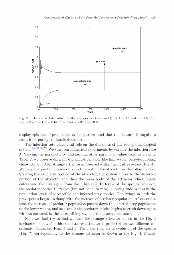
numerical simulation with ψ = 0 and then have compared the results with ψ = 0.First of all we take a set of hypothetical parameter values r = 2.5 day−1,K = 1densities ha−1, A = 0.2 ha per densities, m = 1ha per densities day−1, n = 0.433haper densities day−1, γ = 0.1day−1, h = 2.26ha per densities, θ = 0.008day−1,λ = 2.8 ha per densities day−1. For these set of parameter values we observe thatsystem (3) with ψ = 0 is locally asymptotically stable around the interior equilib-rium point (Fig. 3). But our motivation is to investigate the rich dynamics such aslimit cycles, period-doubling and chaos in system (3) with ψ = 0 and to observe theeffect of density dependent disease-induced mortality on predator population. Forthis we choose a set of parameter values given in the Table 2 and show the dynamicsof system (3) with ψ = 0 and system (3) with ψ = 0 in the following subsections.

5.1. Dynamics of the system (3) for ψ = 0

Chaos is currently of considerable interest in the population dynamics of infectiousdiseases. Mathematically, chaotic dynamics are not devoid of order but displayepisodes of near-cyclic temporal patterns. McCane and Yodzis65 commented thatproductive environment was a prerequisite for a system to support a chaotic dynam-ical behavior. King et al.66 observed that despite the individual nature of organismsand the noisy nature of biological time series, subtle temporal patterns had beendetected in case of chaotic biological populations. They also showed quantitativelythat chaos manifests itself as a tapestry of identifiable and predictable patternswoven together by stochasticity by using data drawn from chaotic insect popula-tions. May67 commented that simple deterministic rules might explain the complexfluctuations observed in animal abundances, led to an intense search for chaos inextant population data.68 In a pair of pioneering contributions to measles diseasedynamics, Schaffer and coworkers69 drew attention to the fact that chaotic dynamics

June 11, 2010 14:13 WSPC/S0218-3390 129-JBS S0218339010003391


0 500 1000 1500 2000 2500 30000

0.2

0.4

0.6

0.8

1

1.2

1.4

1.6

TIME

PO

PU

LA

TIO

N

infected prey

susceptible prey

predator

Fig. 3. The stable distribution of all three species of system (2) for λ = 2.8 and r = 2.5, K =1, A = 0.2,m = 1, n = 0.433, γ = 0.1, h = 2.26, θ = 0.008.

display episodes of predictable cyclic patterns and that this feature distinguishesthem from purely stochastic dynamics.

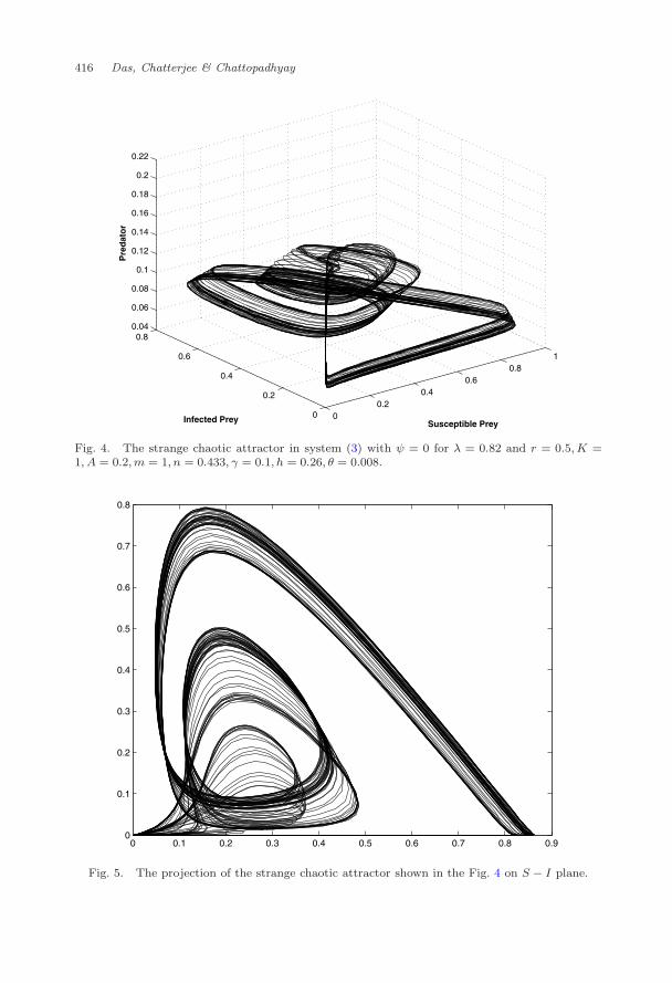
The infection rate plays vital role on the dynamics of any eco-epidemiologicalsystem.3,6,21,59,70 We start our numerical experiments by varying the infection rateλ. Varying the parameter λ, and keeping other parameter values fixed as given inTable 2, we observe different dynamical behavior like limit-cycle, period-doubling,chaos. For λ = 0.82, strange attractor is observed within the positive octant (Fig. 4).We may analyze the motion of trajectory within the attractor in the following way.Starting from the arm portion of the attractor, the system moves to the distortedportion of the attractor and then the main body of the attractor which finallyenters into the arm again from the other side. In terms of the species behavior,the predator species P crashes (but not equal to zero), allowing wide swings in thepopulation levels of susceptible and infected prey species. The swings in both theprey species begins to damp with the increase of predator population. After certaintime the increase of predator population pushes down the infected prey populationto the lower values, and as a result the predator species begins to crash down againwith an outbreak in the susceptible prey, and the process continues.

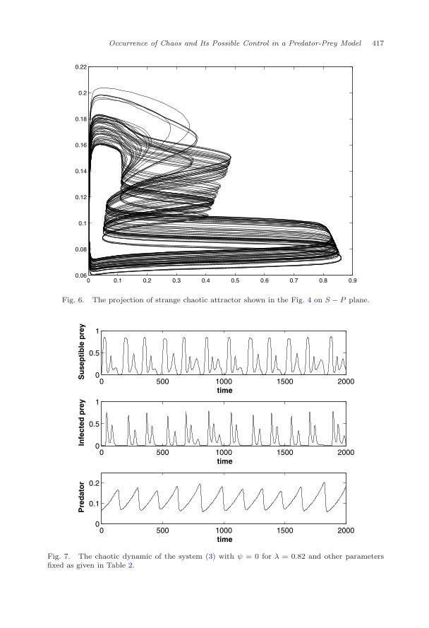
Next we shall try to find whether the strange attractor shown in the Fig. 4is chaotic or not. For this, the strange attractor is projected on two different co-ordinate planes, see Figs. 5 and 6. Then, the time series evolution of the species(Fig. 7) corresponding to the strange attractor is shown in the Fig. 4. Finally

June 11, 2010 14:13 WSPC/S0218-3390 129-JBS S0218339010003391


00.2

0.40.6

0.81

0

0.2

0.4

0.6

0.80.04

0.06

0.08

0.1

0.12

0.14

0.16

0.18

0.2

0.22

Susceptible Prey Infected Prey

Pre

dat

or

Fig. 4. The strange chaotic attractor in system (3) with ψ = 0 for λ = 0.82 and r = 0.5, K =1, A = 0.2,m = 1, n = 0.433, γ = 0.1, h = 0.26, θ = 0.008.

0 0.1 0.2 0.3 0.4 0.5 0.6 0.7 0.8 0.90

0.1

0.2

0.3

0.4

0.5

0.6

0.7

0.8

Fig. 5. The projection of the strange chaotic attractor shown in the Fig. 4 on S − I plane.

June 11, 2010 14:13 WSPC/S0218-3390 129-JBS S0218339010003391


0 0.1 0.2 0.3 0.4 0.5 0.6 0.7 0.8 0.90.06

0.08

0.1

0.12

0.14

0.16

0.18

0.2

0.22

Fig. 6. The projection of strange chaotic attractor shown in the Fig. 4 on S − P plane.

0 500 1000 1500 20000

0.5

1

time

Su

sep

tib

le p

rey

0 500 1000 1500 20000

0.5

1

time

Infe

cted

pre

y

0 500 1000 1500 20000

0.1

0.2

time

Pre

dat

or

Fig. 7. The chaotic dynamic of the system (3) with ψ = 0 for λ = 0.82 and other parametersfixed as given in Table 2.

June 11, 2010 14:13 WSPC/S0218-3390 129-JBS S0218339010003391


0 1000 2000 3000 4000 5000 6000 7000 8000 9000−0.5

−0.4

−0.3

−0.2

−0.1

0

0.1

0.2

0.3

0.4

0.5Dynamics of Lyapunov exponents

Time

Lyap

unov

exp

onen

ts

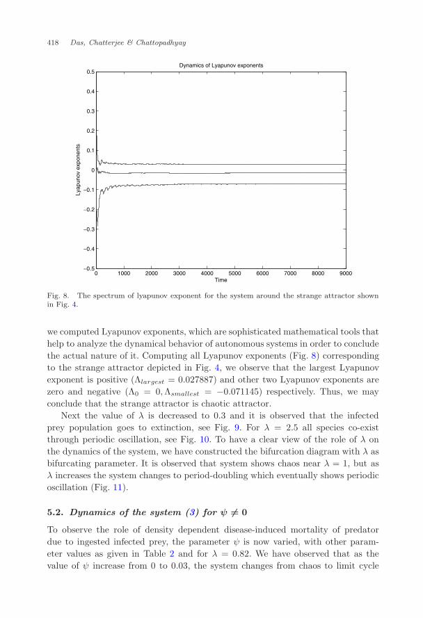
Fig. 8. The spectrum of lyapunov exponent for the system around the strange attractor shownin Fig. 4.

we computed Lyapunov exponents, which are sophisticated mathematical tools thathelp to analyze the dynamical behavior of autonomous systems in order to concludethe actual nature of it. Computing all Lyapunov exponents (Fig. 8) correspondingto the strange attractor depicted in Fig. 4, we observe that the largest Lyapunovexponent is positive (Λlargest = 0.027887) and other two Lyapunov exponents arezero and negative (Λ0 = 0,Λsmallest = −0.071145) respectively. Thus, we mayconclude that the strange attractor is chaotic attractor.

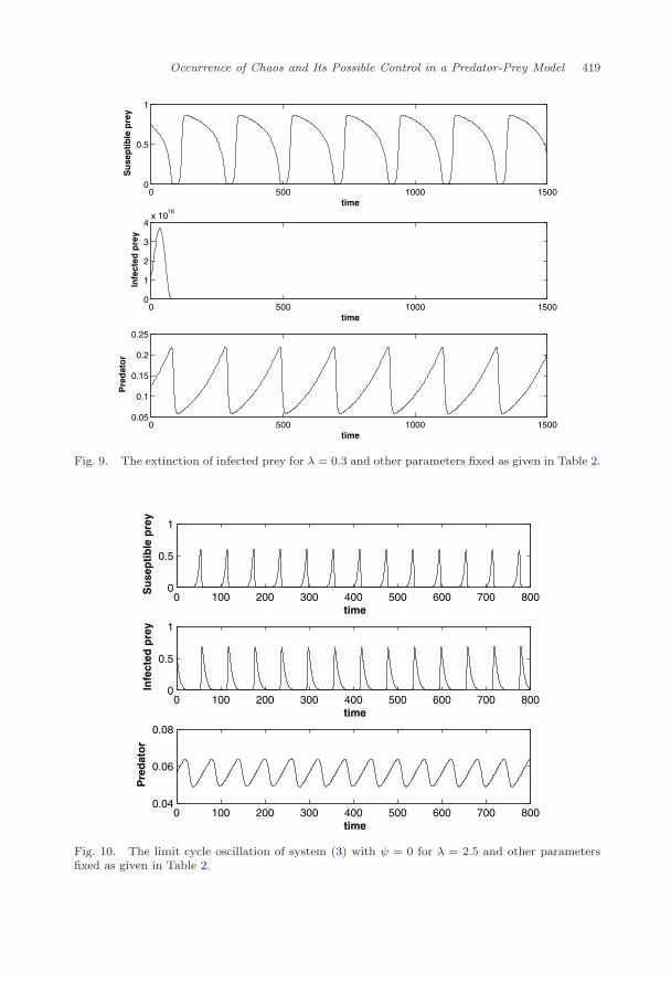
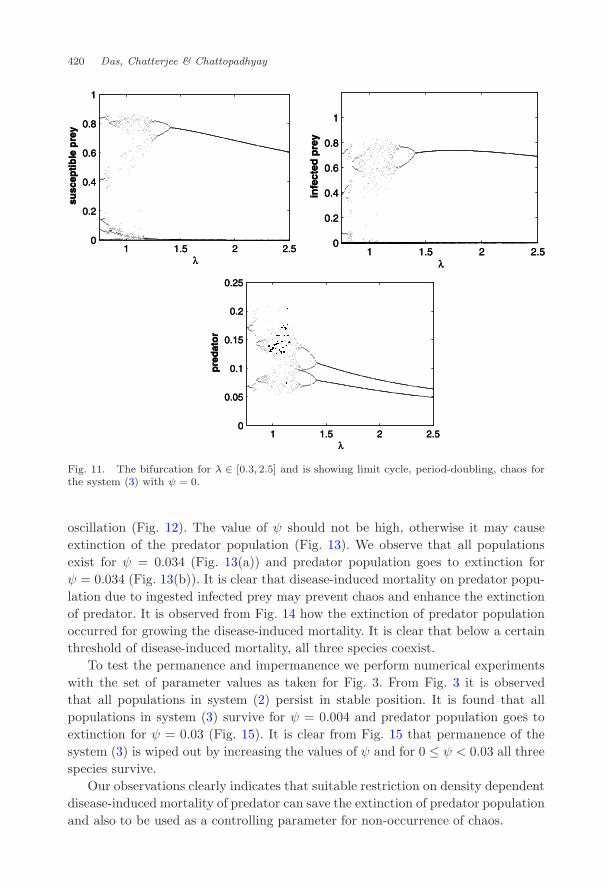
Next the value of λ is decreased to 0.3 and it is observed that the infectedprey population goes to extinction, see Fig. 9. For λ = 2.5 all species co-existthrough periodic oscillation, see Fig. 10. To have a clear view of the role of λ onthe dynamics of the system, we have constructed the bifurcation diagram with λ asbifurcating parameter. It is observed that system shows chaos near λ = 1, but asλ increases the system changes to period-doubling which eventually shows periodicoscillation (Fig. 11).

5.2. Dynamics of the system (3) for ψ = 0

To observe the role of density dependent disease-induced mortality of predatordue to ingested infected prey, the parameter ψ is now varied, with other param-eter values as given in Table 2 and for λ = 0.82. We have observed that as thevalue of ψ increase from 0 to 0.03, the system changes from chaos to limit cycle

June 11, 2010 14:13 WSPC/S0218-3390 129-JBS S0218339010003391


0 500 1000 15000

0.5

1

time

Su

sep

tib

le p

rey

0 500 1000 15000

1

2

3

4x 10

16

time

Infe

cted

pre

y

0 500 1000 15000.05

0.1

0.15

0.2

0.25

time

Pre

dat

or

Fig. 9. The extinction of infected prey for λ = 0.3 and other parameters fixed as given in Table 2.

0 100 200 300 400 500 600 700 8000

0.5

1

time

Su

sep

tib

le p

rey

0 100 200 300 400 500 600 700 8000

0.5

1

time

Infe

cted

pre

y

0 100 200 300 400 500 600 700 8000.04

0.06

0.08

time

Pre

dat

or

Fig. 10. The limit cycle oscillation of system (3) with ψ = 0 for λ = 2.5 and other parametersfixed as given in Table 2.

June 11, 2010 14:13 WSPC/S0218-3390 129-JBS S0218339010003391


1 1.5 2 2.50

0.2

0.4

0.6

0.8

1

λ

su

scep

tib

le p

rey

1 1.5 2 2.50

0.2

0.4

0.6

0.8

1

λ

infe

cted

pre

y

1 1.5 2 2.50

0.05

0.1

0.15

0.2

0.25

λ

pre

dat

or

1 1.5 2 2.50

0.2

0.4

0.6

0.8

1

λ

su

scep

tib

le p

rey

1 1.5 2 2.50

0.2

0.4

0.6

0.8

1

λ

infe

cted

pre

y

1 1.5 2 2.50

0.05

0.1

0.15

0.2

0.25

λ

pre

dat

or

Fig. 11. The bifurcation for λ ∈ [0.3, 2.5] and is showing limit cycle, period-doubling, chaos forthe system (3) with ψ = 0.

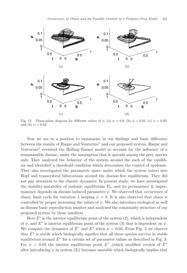
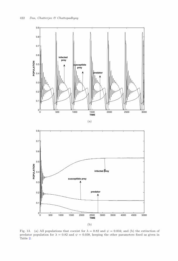
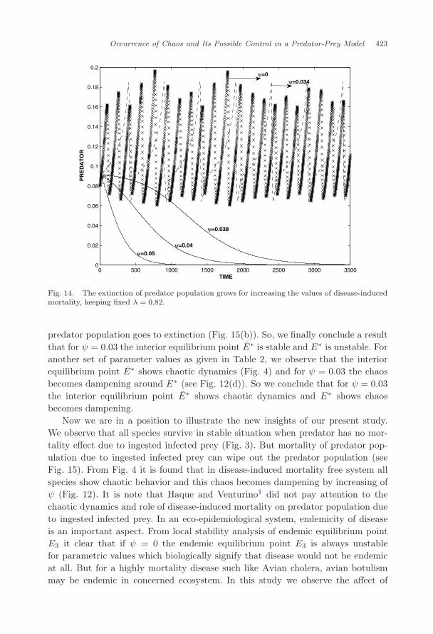
oscillation (Fig. 12). The value of ψ should not be high, otherwise it may causeextinction of the predator population (Fig. 13). We observe that all populationsexist for ψ = 0.034 (Fig. 13(a)) and predator population goes to extinction forψ = 0.034 (Fig. 13(b)). It is clear that disease-induced mortality on predator popu-lation due to ingested infected prey may prevent chaos and enhance the extinctionof predator. It is observed from Fig. 14 how the extinction of predator populationoccurred for growing the disease-induced mortality. It is clear that below a certainthreshold of disease-induced mortality, all three species coexist.

To test the permanence and impermanence we perform numerical experimentswith the set of parameter values as taken for Fig. 3. From Fig. 3 it is observedthat all populations in system (2) persist in stable position. It is found that allpopulations in system (3) survive for ψ = 0.004 and predator population goes toextinction for ψ = 0.03 (Fig. 15). It is clear from Fig. 15 that permanence of thesystem (3) is wiped out by increasing the values of ψ and for 0 ≤ ψ < 0.03 all threespecies survive.

Our observations clearly indicates that suitable restriction on density dependentdisease-induced mortality of predator can save the extinction of predator populationand also to be used as a controlling parameter for non-occurrence of chaos.

June 11, 2010 14:13 WSPC/S0218-3390 129-JBS S0218339010003391


00.5

1

00.5

10

0.05

0.1

SI

P

00.5

1

00.5

10

0.05

0.1

I

P

(a) (b)

00.5

1

00.5

10

0.05

0.1

SI

P

00.5

1

00.5

10

0.05

0.1

SI

P

(c) (d)

Fig. 12. Phase-plane diagram for different values of ψ. (a) ψ = 0.0; (b) ψ = 0.01; (c) ψ = 0.02;and (d) ψ = 0.03.

Now we are in a position to summarize in our findings and basic differencebetween the results of Haque and Venturino1 and our proposed system. Haque andVenturino1 revisited the Holling-Tanner model to account for the influence of atransmissible disease, under the assumption that it spreads among the prey speciesonly. They analyzed the behavior of the system around the each of the equilib-ria and identified a threshold condition which determines the control of epidemic.They also investigated the parametric space under which the system enters intoHopf and transcritical bifurcations around the disease-free equilibrium. They didnot pay attention to the chaotic dynamics. In present study, we have investigatedthe stability-instability of endemic equilibrium E3, and its permanence & imper-manence depends on disease-induced parameter ψ. We observed that occurrence ofchaos, limit cycle for variation λ keeping ψ = 0. It is also observed that chaos iscontrolled by proper increasing the values of ψ. We also introduce ecological as wellas disease basic reproduction number and analyzed the community structure of ourproposed system by these numbers.

Here E∗ is the interior equilibrium point of the system (2), which is independentof ψ, and E∗ is interior equilibrium point of the system (3) that is dependent on ψ.We compare the dynamics of E∗ and E∗ when ψ = 0.03. From Fig. 3 we observethat E∗ is stable which biologically signifies that all three species survive in stableequilibrium around E∗ for a certain set of parameter values as described in Fig. 3.For ψ = 0.03 the interior equilibrium point E∗ (which modified version of E∗

after introducing ψ in system (2)) becomes unstable which biologically implies that

June 11, 2010 14:13 WSPC/S0218-3390 129-JBS S0218339010003391


0 500 1000 1500 2000 2500 30000

0.1

0.2

0.3

0.4

0.5

0.6

0.7

0.8

0.9

TIME

PO

PU

LA

TIO

N

infected prey

susceptible prey

predator

(a)

0 500 1000 1500 2000 2500 3000 3500 4000 4500 50000

0.1

0.2

0.3

0.4

0.5

0.6

0.7

0.8

TIME

PO

PU

LA

TIO

N

infected prey

susceptible prey

predator

(b)

Fig. 13. (a) All populations that coexist for λ = 0.82 and ψ = 0.034; and (b) the extinction ofpredator population for λ = 0.82 and ψ = 0.038, keeping the other parameters fixed as given inTable 2.

June 11, 2010 14:13 WSPC/S0218-3390 129-JBS S0218339010003391


0 500 1000 1500 2000 2500 3000 35000

0.02

0.04

0.06

0.08

0.1

0.12

0.14

0.16

0.18

0.2

TIME

PR

ED

AT

OR

ψ=0ψ=0.034

ψ=0.038

ψ=0.04ψ=0.05

Fig. 14. The extinction of predator population grows for increasing the values of disease-inducedmortality, keeping fixed λ = 0.82.

predator population goes to extinction (Fig. 15(b)). So, we finally conclude a resultthat for ψ = 0.03 the interior equilibrium point E∗ is stable and E∗ is unstable. Foranother set of parameter values as given in Table 2, we observe that the interiorequilibrium point E∗ shows chaotic dynamics (Fig. 4) and for ψ = 0.03 the chaosbecomes dampening around E∗ (see Fig. 12(d)). So we conclude that for ψ = 0.03the interior equilibrium point E∗ shows chaotic dynamics and E∗ shows chaosbecomes dampening.

Now we are in a position to illustrate the new insights of our present study.We observe that all species survive in stable situation when predator has no mor-tality effect due to ingested infected prey (Fig. 3). But mortality of predator pop-ulation due to ingested infected prey can wipe out the predator population (seeFig. 15). From Fig. 4 it is found that in disease-induced mortality free system allspecies show chaotic behavior and this chaos becomes dampening by increasing ofψ (Fig. 12). It is note that Haque and Venturino1 did not pay attention to thechaotic dynamics and role of disease-induced mortality on predator population dueto ingested infected prey. In an eco-epidemiological system, endemicity of diseaseis an important aspect. From local stability analysis of endemic equilibrium pointE3 it clear that if ψ = 0 the endemic equilibrium point E3 is always unstablefor parametric values which biologically signify that disease would not be endemicat all. But for a highly mortality disease such like Avian cholera, avian botulismmay be endemic in concerned ecosystem. In this study we observe the affect of

June 11, 2010 14:13 WSPC/S0218-3390 129-JBS S0218339010003391


0 500 1000 1500 2000 2500 30000

0.2

0.4

0.6

0.8

1

1.2

1.4

1.6

TIME

PO

PU

LA

TIO

N

infected prey

predator

susceptible prey

(a)

0 200 400 600 800 1000 1200 1400 1600 1800 20000

0.2

0.4

0.6

0.8

1

1.2

1.4

1.6

TIME

PO

PU

LA

TIO

N

infected prey

predator susceptible prey

(b)

Fig. 15. (a) The coexistence of all population in stable position for ψ = 0.004; and (b) theextinction of predator population for ψ = 0.03, keeping the other parameters values fixed inFig. 3.

June 11, 2010 14:13 WSPC/S0218-3390 129-JBS S0218339010003391


introducing disease-introducing mortality on the stability of E3. It is found that E3

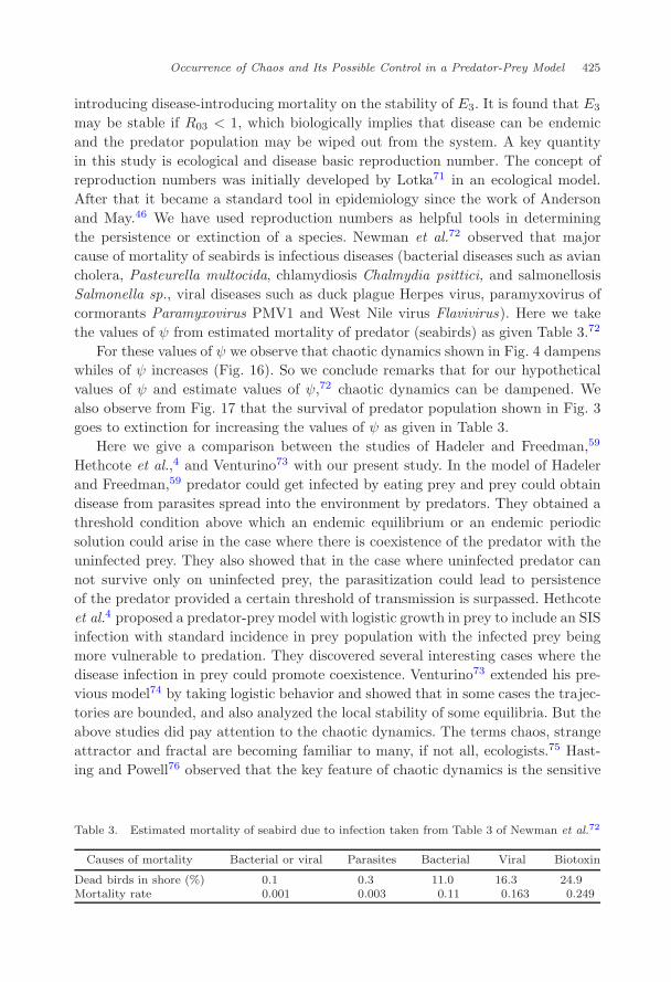
may be stable if R03 < 1, which biologically implies that disease can be endemicand the predator population may be wiped out from the system. A key quantityin this study is ecological and disease basic reproduction number. The concept ofreproduction numbers was initially developed by Lotka71 in an ecological model.After that it became a standard tool in epidemiology since the work of Andersonand May.46 We have used reproduction numbers as helpful tools in determiningthe persistence or extinction of a species. Newman et al.72 observed that majorcause of mortality of seabirds is infectious diseases (bacterial diseases such as aviancholera, Pasteurella multocida, chlamydiosis Chalmydia psittici, and salmonellosisSalmonella sp., viral diseases such as duck plague Herpes virus, paramyxovirus ofcormorants Paramyxovirus PMV1 and West Nile virus Flavivirus). Here we takethe values of ψ from estimated mortality of predator (seabirds) as given Table 3.72

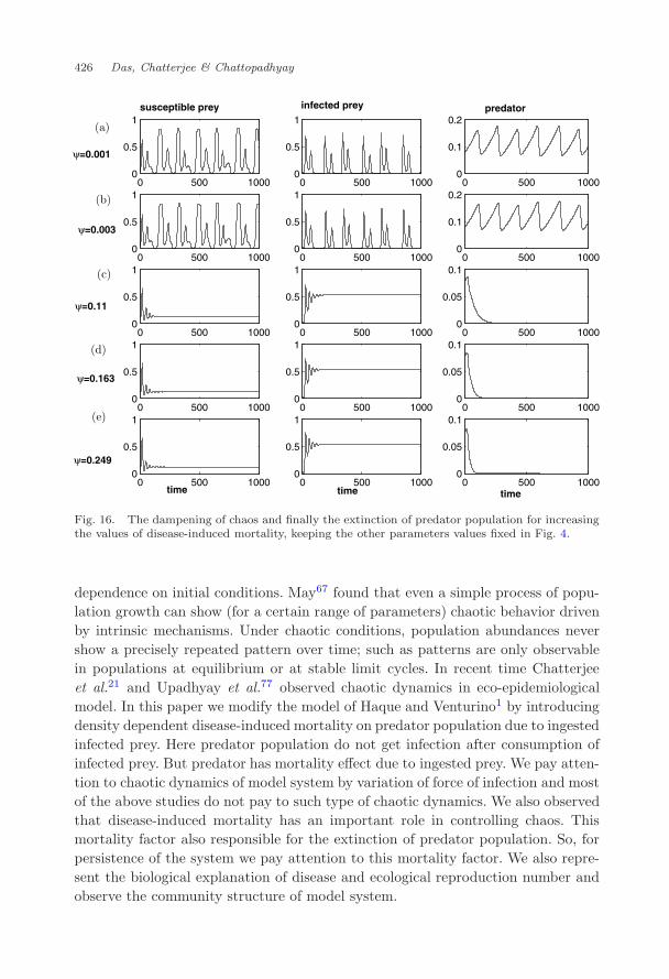
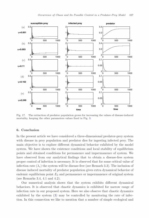
For these values of ψ we observe that chaotic dynamics shown in Fig. 4 dampenswhiles of ψ increases (Fig. 16). So we conclude remarks that for our hypotheticalvalues of ψ and estimate values of ψ,72 chaotic dynamics can be dampened. Wealso observe from Fig. 17 that the survival of predator population shown in Fig. 3goes to extinction for increasing the values of ψ as given in Table 3.

Here we give a comparison between the studies of Hadeler and Freedman,59

Hethcote et al.,4 and Venturino73 with our present study. In the model of Hadelerand Freedman,59 predator could get infected by eating prey and prey could obtaindisease from parasites spread into the environment by predators. They obtained athreshold condition above which an endemic equilibrium or an endemic periodicsolution could arise in the case where there is coexistence of the predator with theuninfected prey. They also showed that in the case where uninfected predator cannot survive only on uninfected prey, the parasitization could lead to persistenceof the predator provided a certain threshold of transmission is surpassed. Hethcoteet al.4 proposed a predator-prey model with logistic growth in prey to include an SISinfection with standard incidence in prey population with the infected prey beingmore vulnerable to predation. They discovered several interesting cases where thedisease infection in prey could promote coexistence. Venturino73 extended his pre-vious model74 by taking logistic behavior and showed that in some cases the trajec-tories are bounded, and also analyzed the local stability of some equilibria. But theabove studies did pay attention to the chaotic dynamics. The terms chaos, strangeattractor and fractal are becoming familiar to many, if not all, ecologists.75 Hast-ing and Powell76 observed that the key feature of chaotic dynamics is the sensitive

Table 3. Estimated mortality of seabird due to infection taken from Table 3 of Newman et al.72

Causes of mortality Bacterial or viral Parasites Bacterial Viral Biotoxin

Dead birds in shore (%) 0.1 0.3 11.0 16.3 24.9Mortality rate 0.001 0.003 0.11 0.163 0.249

June 11, 2010 14:13 WSPC/S0218-3390 129-JBS S0218339010003391


0 500 10000

0.5

1

0 500 10000

0.5

1

0 500 10000

0.1

0.2

0 500 10000

0.5

1

0 500 10000

0.5

1

0 500 10000

0.1

0.2

0 500 10000

0.5

1

0 500 10000

0.5

1

0 500 10000

0.05

0.1

0 500 10000

0.5

1

0 500 10000

0.5

1

0 500 10000

0.05

0.1

0 500 10000

0.5

1

0 500 10000

0.5

1

0 500 10000

0.05

0.1

susceptible prey infected prey predator

time time time

ψ=0.001

ψ=0.003

ψ=0.11

ψ=0.163

ψ=0.249

Fig. 16. The dampening of chaos and finally the extinction of predator population for increasingthe values of disease-induced mortality, keeping the other parameters values fixed in Fig. 4.

dependence on initial conditions. May67 found that even a simple process of popu-lation growth can show (for a certain range of parameters) chaotic behavior drivenby intrinsic mechanisms. Under chaotic conditions, population abundances nevershow a precisely repeated pattern over time; such as patterns are only observablein populations at equilibrium or at stable limit cycles. In recent time Chatterjeeet al.21 and Upadhyay et al.77 observed chaotic dynamics in eco-epidemiologicalmodel. In this paper we modify the model of Haque and Venturino1 by introducingdensity dependent disease-induced mortality on predator population due to ingestedinfected prey. Here predator population do not get infection after consumption ofinfected prey. But predator has mortality effect due to ingested prey. We pay atten-tion to chaotic dynamics of model system by variation of force of infection and mostof the above studies do not pay to such type of chaotic dynamics. We also observedthat disease-induced mortality has an important role in controlling chaos. Thismortality factor also responsible for the extinction of predator population. So, forpersistence of the system we pay attention to this mortality factor. We also repre-sent the biological explanation of disease and ecological reproduction number andobserve the community structure of model system.

June 11, 2010 14:13 WSPC/S0218-3390 129-JBS S0218339010003391


0 500 10000

0.5

0 500 10000

1

2

0 500 10000

0.2

0.4

0 500 10000

0.5

0 500 10000

1

2

0 500 10000

0.2

0.4

0 500 10000

0.5

0 500 10000

1

2

0 500 10000

0.05

0.1

0 500 10000

0.5

0 500 10000

1

2

0 500 10000

0.05

0.1

0 500 10000

0.5

0 500 10000

1

2

0 500 10000

0.05

0.1

susceptible prey infected prey predator

time time time

ψ=0.001

ψ=0.003

ψ=0.11

ψ=0.163

ψ=0.249

Fig. 17. The extinction of predator population grows for increasing the values of disease-inducedmortality, keeping the other parameters values fixed in Fig. 3.

6. Conclusion

In the present article we have considered a three-dimensional predator-prey systemwith disease in prey population and predator dies for ingesting infected prey. Themain objective is to explore different dynamical behavior exhibited by the modelsystem. We have shown the existence conditions and local stability of equilibriumpoints and obtained conditions for permanence and impermanence of system. Wehave observed from our analytical findings that to obtain a disease-free systemproper control of infection is necessary. It is observed that for some critical value ofinfection rate (λc) the system will be disease-free (see Remark 3.3). The inclusion ofdisease induced mortality of predator population gives extra dynamical behavior ofendemic equilibrium point E3 and permanence or impermanence of original system(see Remarks 3.4, 4.1 and 4.2).

Our numerical analysis shows that the system exhibits different dynamicalbehaviors. It is observed that chaotic dynamics is exhibited for narrow range ofinfection rate in our proposed system. Here we also observe that chaotic dynamicsexhibited by the system (3) may be controlled by monitoring the rate of infec-tion. In this connection we like to mention that a number of simple ecological and

June 11, 2010 14:13 WSPC/S0218-3390 129-JBS S0218339010003391


epidemiological systems with seasonality in contact rates unequivocally demon-strate chaos.75 Schaffer and Kot78 and Olsen et al.79 show that measles in NewYork, Baltimore and Denmark may be a specific example of this behavior. Ander-son and May3 showed that invasion of a resident predator-prey system by a newstrain of parasites could cause destabilization and exhibits limit cycle oscillation.Chattopadhyay et al.80 also showed that in a classical eco-epidemiological modelforce of infection has an important role in producing periodic oscillation. It is ourinterpretation that chaos ultimately arises in this type of eco-epidemiological modelbecause of the tendency for predator-prey system with disease propagation throughprey species to oscillate. Actually chaos arises when the period of oscillation of inter-acting species for variation of force infection is not multiple of the other frequency(i.e. the frequencies of oscillating species are incommensurate). To support ourinterpretation of chaos we like to mention that Hastings and Powell76 explained thearisen of chaos in tri-trophic food chain model. The interaction at the higher trophiclevels has a longer natural period because the average life time of the top predatorsis longer than the average lifetime of the consumers at the lower trophic levels. Thetwo systems are coupled through intermediate species because the predator in one isprey on the other. The incommensurate frequencies of oscillation of two subsystemsarises chaos. We also observed that the occurrence of the chaos for certain value offorce of infection may also be controlled by introducing disease-induced mortalityof predator due to ingested infected prey. The introduction of the disease-inducedmortality of predators due to ingested infected preys should be low, otherwise itmay cause extinction of the predator population. The extinction of predator due todisease-induced mortality is well in accordance with the results. For example, it isseen that Avian botulism kills thousands of waterbirds annually throughout NorthAmerica but management efforts to reduce its effects have been hindered becauseenvironmental conditions that promote outbreaks are poorly understood.81 TheGreat Salt Lake (GSL) marshes of Utah are important staging areas for migratingshorebirds and waterfowl and are sites of intensive management to ensure availabil-ity of highly quality habitats for the migrating birds that use the area82 Howeversevere Avian botulism outbreaks are common in marshes along the eastern shore ofthe GSL83 and have been recorded since 1915.84 These marshes were the site of amajor outbreak in 1997 when approximately 400,000 birds died on the Bear RiverDelta. Throughout the study it has been shown that the density dependent disease-induced mortality of predator due to ingested infected prey may cause extinction ofthe predator population. Our findings also show that the presence of this disease-induced mortality is an important factor for the non-occurrence of chaos of suchsystems.

There is ample room to modify our model equations. As the model dealswith susceptible and infected prey, one can easily modify the system equationsby taking into consideration the food value concept. Moreover, the delay occursin most of the biological process, hence one can modify our model by including

June 11, 2010 14:13 WSPC/S0218-3390 129-JBS S0218339010003391


delay in disease transmission term. We leave these modifications for our futureconsideration.

Acknowledgments

The authors are grateful to the associate editor and the learned reviewers for theircritical comments and suggestions which have immensely improved the content andpresentation of this version.

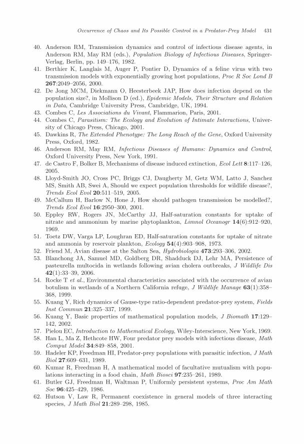
References

1. Haque M, Venturino E, The role of transmissible diseases in the Holling-Tannerpredator-prey model, Theor Popul Biol 70:273–288, 2006.

2. Kermack WO, McKendrick AG, Contributions to the mathematical theory of epi-demics, part 1, Proc R Soc Lond Ser A 115:700–721, 1927.

3. Anderson RM, May RM, The invasion, persistence and spread of infectious diseaseswithin animal and plant communities, Philos Trans R Soc Lond B 314:533–570,1986.

4. Hethcote HW, Wang W, Han L, Ma Z, A predator-prey model with infected prey,Theor Popul Biol 66:259–268, 2004.

5. Dobson AP, The population biology of parasite induced changes in host behaviour,Quart Rev Biol 63:139–165, 1988.

6. Chattopadhyay J, Arino O, A predator-prey model with disease in the prey, NonlinAnal 36:747–766, 1999.

7. Hall SR, Duffy MA, Caceres CE, Selective predation and productivity jointly drivecomplex behavior in host-parasite systems, Am Nat 165(1):70–81, 2005.

8. Sih A, Crowley P, McPeek M, Petranka J, Strohmeier K, Predation, competition andprey communities: a review of field experiments, Annu Rev Ecol Syst 16:269–311,1985.

9. Dwyer G, Dushoff J, Yee SH, Generalist predators, specialist pathogens and insectoutbreaks, Nature 43:341–345, 2004.

10. Hudson PJ, Dobson AP, Newborn D, Prevention of population cycles by parasiteremoval, Science 282:2256–2258, 1998.

11. Ives AR, Murray DL, Can sublethal parasitism destabilize predator-prey populationdynamics? A model of snowshoe hares predators and parasites, J Anim Ecol 66:265–278, 1997.

12. Packer C, Holt RD, Hudson PJ, Lafferty KD, Dobson AP, Keeping the herbs healtyand alert: implications of predator control for infection disease, Ecol Lett 6:792–802,2003.

13. Temple SA, Do predators always capture substandard individuals disproportionatelyfrom prey populations? Ecology 68:669–674, 1987.

14. Van Dobben WH, The food of cormorants in the Netherlands, Ardea 40:1–63, 1952.15. Vaughn GE, Coble PW, Sublethal effects of three ectoparasites on fish, J Fish Biol

7:283–294, 1975.16. Holmes JC, Bethel WM, Modification of intermediate host behavior by parasites, in

Canning EU, Wright CA (eds.), Behavioral Aspects of Parasite Transmission, Aca-demic Press, London, pp. 123–149, 1972.

June 11, 2010 14:13 WSPC/S0218-3390 129-JBS S0218339010003391


17. Lafferty KD, Morhis AK, Altered behavior of parasited killifish increase susceptibleto predation by binal final hosts, Ecology 77:1390–1397, 1996.

18. Brattey J, The effects of larval Acanthocephalus licii on the propogation reproductionand susceptibility to predation of the isopod Ascellus Aquaticus, J Parasitol 69:1172–1173, 1983.

19. Chattopadhyay J, Srinivasu PDN, Bairagi N, Pelicans at risk in Salton Sea — aneco-epidemiological model-II, Ecol Model 167:199–211, 2003.

20. Chattopadhyay J, Bairagi N, Pelicans at risk in Salton Sea — an eco-epidemiologicalmodel, Ecol Model 136:103–112, 2001.

21. Chatterjee S, Bandyopadhyay M, Chattopadhyay J, Proper predation makes the sys-tem disease free — conclusion drawn from an eco-epidemiological model, J Biol Syst14(4):599–616, 2006.

22. Earn DJD, Rohani P, Bolker BM, Grenfell B, A simple model for complex dynamicaltransitions in epidemics, Science 287:667–670, 2000.

23. Schwartz IB, Smith HL, Infinite subharmonic bifurcation in an SEIR epidemic model,J Math Biol 18:233–253, 1983.

24. Arditi R, Ginzburg LR, Coulping in predator-prey dynamics: ratio-dependence, JTheor Biol 139:311–326, 1989.

25. Abrams PA, The fallacies of ratio-dependent predation, Ecology 75:1842–1850, 1994.26. Abrams PA, Anomalous predictions of ratio-dependent models of predation, Oikos

80:163–171, 1997.27. Abrams PA, Ginzburg LR, The nature of predation prey dependent, ratio dependent,

or neither? Trends Ecol Evol 15:337–341, 2000.28. Akcakaya HR, Arditi R, Ginzburg LR, Ratio-dependent predation: an abstraction

that works, Ecology 76:995–1004, 1995.29. Arditi R, Ginzburg LR, Akcakaya HR, Variation in plankton densities among lakes:

a case for ratio-dependent models, Am Nat 138:1287–1296, 1991.30. Arditi R, Saiah H, Emperical evidence of the role of heterogeneity in ratio-dependent

consumption, Ecology 73:1544–1551, 1992.31. Arditi R, Berryman AA, The biological paradox, Trends Ecol Evol 6:32, 1991.32. DeAngelis DL, Holland JN, Emergence of ratio-dependent and predator-dependent

functional responses for pollination mutualism and seed parasitism, Ecol Model191:551–556, 2006.

33. Kuang Y, Beretta A, Global qualitative analysis of a ratio-dependent predatorpreysystems, J Math Biol 35:389–406, 1998.

34. Jost C, Arino O, Arditi R, About deterministic extinction in ratio-dependentpredator–prey models, Bull Math Biol 61:19–32, 1999.

35. Xiao D, Ruan S, Global dynamics of a ratio-dependent predator-prey system, J MathBiol 43:268–290, 2001.

36. Berezovskaya FS, Karev G, Arditi R, Parametric analysis of the ratio-dependentpredator-prey system, J Math Biol 43:221, 2001.

37. Arino O, Abdllaoui A, Mikram J, Chattopadhyay J, Infection on prey populationmay act as a biological control in ratio-dependent predator-prey model, Nonlinearity17:1101–1116, 2004.

38. Hamilton WD, Axelrod R, Tanese R, Sexual reproduction as an adaptation to resistparasites, Proc Nat Acad Sci USA 87:3566–3573, 1990.

39. Uhling G, Sahling G, Long-term studies on Noctiluca scintillans in the German bightpopulation dynamics and red tide phenomena, Neth. J. Sea Res. 25:101–112, 1992.

June 11, 2010 14:13 WSPC/S0218-3390 129-JBS S0218339010003391


40. Anderson RM, Transmission dynamics and control of infectious disease agents, inAnderson RM, May RM (eds.), Population Biology of Infectious Diseases, Springer-Verlag, Berlin, pp. 149–176, 1982.

41. Berthier K, Langlais M, Auger P, Pontier D, Dynamics of a feline virus with twotransmission models with exponentially growing host populations, Proc R Soc Lond B267:2049–2056, 2000.

42. De Jong MCM, Diekmann O, Heesterbeek JAP, How does infection depend on thepopulation size?, in Mollison D (ed.), Epidemic Models, Their Structure and Relationin Data, Cambridge University Press, Cambridge, UK, 1994.

43. Combes C, Les Associations du Vivant, Flammarion, Paris, 2001.44. Combes C, Parasitism: The Ecology and Evolution of Intimate Interactions, Univer-

sity of Chicago Press, Chicago, 2001.45. Dawkins R, The Extended Phenotype: The Long Reach of the Gene, Oxford University

Press, Oxford, 1982.46. Anderson RM, May RM, Infectious Diseases of Humans: Dynamics and Control,

Oxford University Press, New York, 1991.47. de Castro F, Bolker B, Mechanisms of disease induced extinction, Ecol Lett 8:117–126,

2005.48. Lloyd-Smith JO, Cross PC, Briggs CJ, Daugherty M, Getz WM, Latto J, Sanchez

MS, Smith AB, Swei A, Should we expect population thresholds for wildlife disease?,Trends Ecol Evol 20:511–519, 2005.

49. McCallum H, Barlow N, Hone J, How should pathogen transmission be modelled?,Trends Ecol Evol 16:2950–300, 2001.

50. Eppley RW, Rogers JN, McCarthy JJ, Half-saturation constants for uptake ofnitrate and ammonium by marine phytoplankton, Limnol Oceanogr 14(6):912–920,1969.

51. Toetz DW, Varga LP, Loughran ED, Half-saturation constants for uptake of nitrateand ammonia by reservoir plankton, Ecology 54(4):903–908, 1973.

52. Friend M, Avian disease at the Salton Sea, Hydrobiologia 473:293–306, 2002.53. Blanchong JA, Samuel MD, Goldberg DR, Shadduck DJ, Lehr MA, Persistence of

pasteurella multocida in wetlands following avian cholera outbreaks, J Wildlife Dis42(1):33–39, 2006.

54. Rocke T et al., Environmental characteristics associated with the occurrence of avianbotulism in wetlands of a Northern California refuge, J Wildlife Manage 63(1):358–368, 1999.

55. Kuang Y, Rich dynamics of Gause-type ratio-dependent predator-prey system, FieldsInst Commun 21:325–337, 1999.

56. Kuang Y, Basic properties of mathematical population models, J Biomath 17:129–142, 2002.

57. Pielou EC, Introduction to Mathematical Ecology, Wiley-Interscience, New York, 1969.58. Han L, Ma Z, Hethcote HW, Four predator prey models with infectious disease, Math

Comput Model 34:849–858, 2001.59. Hadeler KP, Freedman HI, Predator-prey populations with parasitic infection, J Math

Biol 27:609–631, 1989.60. Kumar R, Freedman H, A mathematical model of facultative mutualism with popu-

lations interacting in a food chain, Math Biosci 97:235–261, 1989.61. Butler GJ, Freedman H, Waltman P, Uniformly persistent systems, Proc Am Math

Soc 96:425–429, 1986.62. Hutson V, Law R, Permanent coexistence in general models of three interacting

species, J Math Biol 21:289–298, 1985.

June 11, 2010 14:13 WSPC/S0218-3390 129-JBS S0218339010003391


63. Hofbauer J, Saturated equilibria, permanence and stability for ecological systems,in Groos L, Hallam T, Levin S (eds.), Mathematical Ecology, Proc. Trieste, WorldScientific, Singapore, 1986.

64. Alpine AE, Cloern JE, Phytoplankton growth rates in a light-limited environment,San Francisco Bay Mar Ecol Prog Ser 44:167–173, 1988.

65. Mccann K, Yodzis P, Bifurcation structure of a three-species food-chain model, TheorPopul Biol 48:93–125, 1995.

66. King et al., Anatomy of a chaotic attractor: subtle model predicted patterns revealedin population data, Proc Natl Acad Sci USA 101:408–413, 2004.

67. May RM, Simple mathematical models with very complicated dynamics, Nature261:4590-467, 1976.

68. Schaffer WM, Stretching and folding in lynx for attractor in nature? Am Nat 124:798–820, 1984.

69. Schaffer WM, Transient periodicity and episodic predicability in biological dynamics.IMA J Math Appl Med Biol 10:227–247, 1993.

70. Freedman HI, A model of predator-prey dynamics modified by the action of parasite,Math Biosci 99:143–155, 1990.

71. Lotka AJ, Relation between birth rates and death rates, Science 26:21–22, 1925.72. Newman SH, Chmura A, Converse K, Kilpatrick AM, Patel N, Lammers E, Daszak

P, Aquatic bird disease and mortality as an indicator of changing ecosystem health,Mar Ecol Prog Ser 352:299–309, 2007.

73. Venturino E, Epidemics in predator-prey model: disease in the predators, IMA J MathAppl Med Biol 19:185–205, 2002.

74. Venturino E, The influence of diseases on Lotka Volterra systems, Rocky Mt J Math24:381–402, 1994.

75. Schaffer WM, Kot M, Chaos in ecological systems the coals that Newcastle forgot,Trends Ecol Evol 1:58–63, 1986.

76. Hastings A, Powell T, Chaos in three-species food chain, Ecology 72(3):896–903, 1991.77. Upadhyay R, Bairagi N, Kundu K, Chattopadhyay J, Chaos in eco-epidemiological

problem of Salton Sea and its possible control, Appl Math Comput 196(1):392–401,2008.

78. Schaffer WM, Kot M, Do strange attractors govern ecological systems? BioScience35:342–350, 1985.

79. Olsen LF, Truty GL, Schaffer WM, Oscillations and chaos in epidemics: a non-lineardynamic study of six childhood diseases in Copenhagen, Denmark Theor Popul Biol33:344–370, 1988.

80. Chattopadhyay J, Pal S, El Abdllaoui A, Classical predator-prey system with infectionof prey population — a mathematical model, Math Meth Appl Sci 26:1211–1222, 2003.

81. Tonie ER, Michael DS, Water and sediment characteristics associated with Avianbotulism outbreaks in wetlands, J Wildlife Manage 63(4):1249–1260, 1999.

82. Kadlec JA, Smith LM, Great Basin marshes, in Smith LM, Pederson RL, KaminskiRM (eds.), Habitat Management for Migrating and Wintering Waterfowl in NorthAmerica, Texas Tech University, Lubbock, USA, pp. 451–474, 1989.

83. Rosen MN, Botulism, in Davis JW, Anderson RC, Karstad L, Trainer DO (eds.),Infectious and Parasitic Diseases of Wild Birds, Iowa State University, Ames, USA,pp. 100–117, 1971.

84. Wetmore A, The Duck Sickness in Utah, United States Department of AgricultureBulletin Series No. 672, pp. 1–26, 1918.

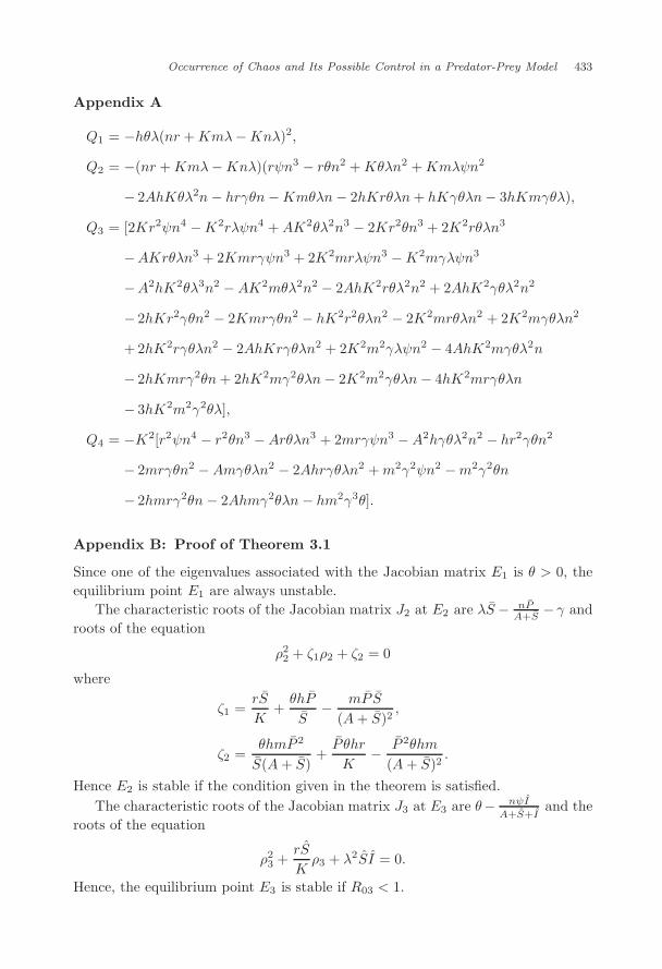
June 11, 2010 14:13 WSPC/S0218-3390 129-JBS S0218339010003391


Appendix A

Q1 = −hθλ(nr +Kmλ−Knλ)2,

Q2 = −(nr +Kmλ−Knλ)(rψn3 − rθn2 +Kθλn2 +Kmλψn2

− 2AhKθλ2n− hrγθn−Kmθλn− 2hKrθλn+ hKγθλn− 3hKmγθλ),

Q3 = [2Kr2ψn4 −K2rλψn4 +AK2θλ2n3 − 2Kr2θn3 + 2K2rθλn3

−AKrθλn3 + 2Kmrγψn3 + 2K2mrλψn3 −K2mγλψn3

−A2hK2θλ3n2 −AK2mθλ2n2 − 2AhK2rθλ2n2 + 2AhK2γθλ2n2

− 2hKr2γθn2 − 2Kmrγθn2 − hK2r2θλn2 − 2K2mrθλn2 + 2K2mγθλn2

+ 2hK2rγθλn2 − 2AhKrγθλn2 + 2K2m2γλψn2 − 4AhK2mγθλ2n

− 2hKmrγ2θn+ 2hK2mγ2θλn− 2K2m2γθλn− 4hK2mrγθλn

− 3hK2m2γ2θλ],

Q4 = −K2[r2ψn4 − r2θn3 −Arθλn3 + 2mrγψn3 −A2hγθλ2n2 − hr2γθn2

− 2mrγθn2 −Amγθλn2 − 2Ahrγθλn2 +m2γ2ψn2 −m2γ2θn

− 2hmrγ2θn− 2Ahmγ2θλn− hm2γ3θ].

Appendix B: Proof of Theorem 3.1

Since one of the eigenvalues associated with the Jacobian matrix E1 is θ > 0, theequilibrium point E1 are always unstable.

The characteristic roots of the Jacobian matrix J2 at E2 are λS − nPA+S

− γ androots of the equation

ρ22 + ζ1ρ2 + ζ2 = 0

where

ζ1 =rS

K+θhP

S− mP S

(A+ S)2,

ζ2 =θhmP 2

S(A+ S)+P θhr

K− P 2θhm

(A+ S)2.

Hence E2 is stable if the condition given in the theorem is satisfied.The characteristic roots of the Jacobian matrix J3 at E3 are θ− nψI

A+S+Iand the

roots of the equation

ρ23 +

rS

Kρ3 + λ2SI = 0.

Hence, the equilibrium point E3 is stable if R03 < 1.

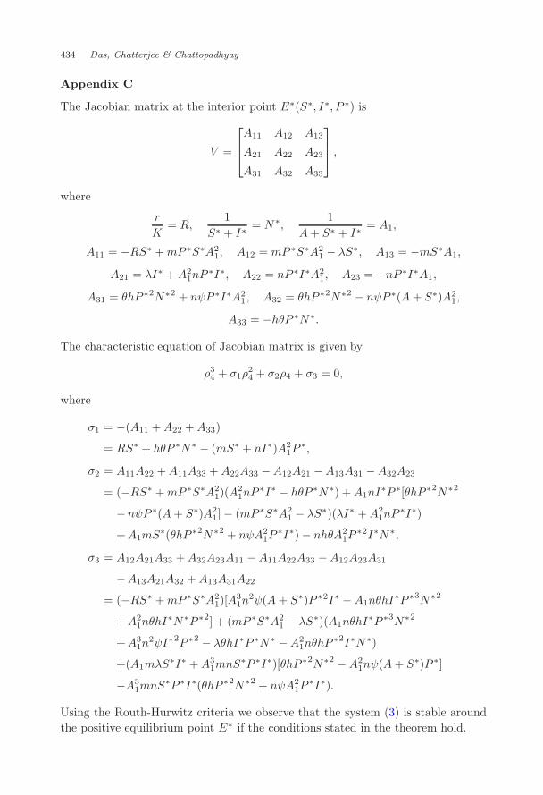
June 11, 2010 14:13 WSPC/S0218-3390 129-JBS S0218339010003391


Appendix C

The Jacobian matrix at the interior point E∗(S∗, I∗, P ∗) is

V =

A11 A12 A13

A21 A22 A23

A31 A32 A33

,

where

r

K= R,

1S∗ + I∗

= N∗,1

A+ S∗ + I∗= A1,

A11 = −RS∗ +mP ∗S∗A21, A12 = mP ∗S∗A2

1 − λS∗, A13 = −mS∗A1,

A21 = λI∗ +A21nP

∗I∗, A22 = nP ∗I∗A21, A23 = −nP ∗I∗A1,

A31 = θhP ∗2N∗2 + nψP ∗I∗A21, A32 = θhP ∗2N∗2 − nψP ∗(A+ S∗)A2

1,

A33 = −hθP ∗N∗.

The characteristic equation of Jacobian matrix is given by

ρ34 + σ1ρ

24 + σ2ρ4 + σ3 = 0,

where

σ1 = −(A11 +A22 +A33)

= RS∗ + hθP ∗N∗ − (mS∗ + nI∗)A21P

∗,

σ2 = A11A22 +A11A33 +A22A33 −A12A21 −A13A31 −A32A23

= (−RS∗ +mP ∗S∗A21)(A

21nP

∗I∗ − hθP ∗N∗) +A1nI∗P ∗[θhP ∗2N∗2

−nψP ∗(A+ S∗)A21] − (mP ∗S∗A2

1 − λS∗)(λI∗ +A21nP

∗I∗)

+A1mS∗(θhP ∗2N∗2 + nψA2

1P∗I∗) − nhθA2

1P∗2I∗N∗,

σ3 = A12A21A33 +A32A23A11 −A11A22A33 −A12A23A31

−A13A21A32 +A13A31A22

= (−RS∗ +mP ∗S∗A21)[A

31n

2ψ(A+ S∗)P ∗2I∗ −A1nθhI∗P ∗3N∗2

+A21nθhI

∗N∗P ∗2] + (mP ∗S∗A21 − λS∗)(A1nθhI

∗P ∗3N∗2

+A31n

2ψI∗2P ∗2 − λθhI∗P ∗N∗ −A21nθhP

∗2I∗N∗)

+(A1mλS∗I∗ +A3

1mnS∗P ∗I∗)[θhP ∗2N∗2 −A2

1nψ(A+ S∗)P ∗]

−A31mnS

∗P ∗I∗(θhP ∗2N∗2 + nψA21P

∗I∗).

Using the Routh-Hurwitz criteria we observe that the system (3) is stable aroundthe positive equilibrium point E∗ if the conditions stated in the theorem hold.

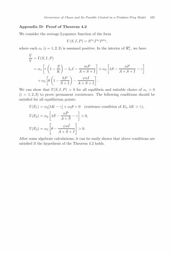
June 11, 2010 14:13 WSPC/S0218-3390 129-JBS S0218339010003391


Appendix D: Proof of Theorem 4.2

We consider the average Lyapunov function of the form

V (S, I, P ) = Sα1Iα2Pα3 ,

where each αi (i = 1, 2, 3) is assumed positive. In the interior of 3+, we have

V

V= Γ(S, I, P )

= α1

[r

(1 − S

K

)− λ1I − mP

A+ S + I

]+ α2

[λS − nP

A+ S + I− γ

]

+α3

[θ

(1 − hP

S + I

)− ψnI

A+ S + I

].

We can show that Γ(S, I, P ) > 0 for all equilibria and suitable choice of αi > 0(i = 1, 2, 3) to prove permanent coexistence. The following conditions should besatisfied for all equilibrium points:

Γ(E1) = α2[λK − γ] + α3θ > 0 (existence condition of E3, λK > γ),

Γ(E2) = α2

[λS − nP

A+ S− γ

]> 0,

Γ(E3) = α3

[θ − ψnI

A+ S + I

]> 0.

After some algebraic calculations, it can be easily shown that above conditions aresatisfied if the hypothesis of the Theorem 4.2 holds.

occurrence of chaos and its possible control in a predator-prey model with density dependent...

Documents