smoothviz: visualization of smoothed particles hydrodynamics data

0

SmoothViz: Visualization of Smoothed ParticlesHydrodynamics Data

Lars Linsen1, Vladimir Molchanov1, Petar Dobrev1, Stephan Rosswog1,Paul Rosenthal2 and Tran Van Long3

1Jacobs University, Bremen2Chemnitz University of Technology

3University of Transport and Communication, Hanoi1,2Germany

3Vietnam

1. Introduction

Smoothed particle hydrodynamics (SPH) is a completely mesh-free method to simulatefluid flow (Gingold & Monaghan, 1977; Lucy, 1977). Rather than representing the physicalvariables on a fixed grid, the fluid is represented by freely moving interpolation centers(“particles”). Apart from their position and velocity these particles carry information aboutthe physical quantities of the considered fluid, such as temperature, composition, chemicalpotentials, etc. As the method is completely Lagrangian and particles follow the motion of theflow, the particles represent an unstructured data set at each point in time, i.e., the particles donot exhibit a regular spatial arrangement nor a fixed connectivity. For a recent detailed reviewof modern formulations of the SPH method see Rosswog (2009).For the analysis of the simulation results, data visualization plays an important role.However, visualization methods need to account for the highly adaptive, unstructured datarepresentation in SPH simulations. Reconstructing the entire data field over a regular grid isnot an option, as it would either use grids of immense sizes that cannot be handled efficientlyanymore or it inevitably would introduce significant interpolation errors. Such errors shouldbe avoided, especially as they would occur most prominently in areas of high particle density,i.e., areas of highest importance are undersampled. Adaptive grids may be an option asinterpolation errors can be kept low, but the adaptivity requires special treatments duringthe visualization process.In this chapter, we introduce visualization methods that operate directly on the particledata, i.e., on unstructured point-based volumetric data. Section 3 introduces an approachto directly extract isosurfaces from a scalar field of the SPH simulation. Isosurfaces extractionis a common visualization concept and is suitable for SPH data visualization, as one is ofteninterested in seeing boundaries of certain features.Because of the use of radial kernel functions in SPH computations (which is crucial forexact conservation of energy, momentum, and angular momentum) together with a poora resolution, one can observe that the extracted isosurfaces may be bumpy, especially inregions of low particle density. We approach this issue by introducing level-set methods for

1

www.intechopen.com

https://www.researchgate.net/publication/231514047_Smoothed_Particle_Hydrodynamics_-_Theory_and_Application_to_Non-Spherical_Stars?el=1_x_8&enrichId=rgreq-aebbad6f-e49b-4e37-ba27-e88d76466a42&enrichSource=Y292ZXJQYWdlOzIyMTkwNTk4OTtBUzo5NzM0NjY0NTkyMTgwMEAxNDAwMjIwNjU3NTE0

https://www.researchgate.net/publication/231514049_Lucy_LB_Numerical_approach_to_testing_of_fission_hypothesis_Astron_J_8212_1013-1024?el=1_x_8&enrichId=rgreq-aebbad6f-e49b-4e37-ba27-e88d76466a42&enrichSource=Y292ZXJQYWdlOzIyMTkwNTk4OTtBUzo5NzM0NjY0NTkyMTgwMEAxNDAwMjIwNjU3NTE0

2 Will-be-set-by-IN-TECH

scalar field segmentation that include a smoothing term and extracting isosurfaces from thesmooth level-set function. Again, the level-set method is only operating on the positions ofthe particles and does not use any auxiliary grid to perform the computations. In Section 4,we describe the general approach of smooth isosurface extraction from SPH data based onlevel-set segmentation and in Section 5, we detail methods for improving the speed of thelevel-set approach narrow-band processing, a local isosurface extraction approach based onvariational level sets, and a non-iterative second-order approximation of the signed distancefunction which is needed throughout the level-set processing.The surfaces that are extracted from particle data are in form of a point cloud representation.Point-based rendering methods that display such surfaces without the necessity to firstgenerate a triangular mesh from the point clouds have become popular in computergraphics within the last decades. We have developed an approach that uses image-spaceoperations to create desired renderings of large point clouds at interactive rates withoutany pre-computations, i.e., not even computing neighborhoods of points. This property isdesirable, as we want to interactively extract different surfaces and display them immediately.Section 6 provides the description of our approach including rendering features such astransparency and shadows.Since SPH simulations include a multitude of fields, it is of interest to investigate themsimultaneously and to explore their correlations. In Section 7, we investigate how multi-fieldfeatures can be detected and visualized. Detection is based on a clustering in themulti-dimensional attribute space. The hierarchy of density clusters can be investigated usingcoordinated views of the cluster tree, parallel coordinates of the multi-dimensional attributespace, and a visualization of the volumetric physical space. The features are displayed inphysical space using surface extraction and rendering.Finally, in Section 8, we explain how multiple scalar and volume fields can be exploredinteractively using a visual system based on the methods described in this chapter. Inaddition to the methods already mentioned, we support some further common visualizationfunctionality for scalar and vector fields.

2. Related work

In the astrophysics SPH community, visualization of slices through the volume, isosurfaceextraction, direct volume rendering techniques, and particle rendering as color-mappedpoints are most commonly used for the display of single scalar fields (Navratil et al., 2007;Walker et al., 2005). A tool that provides such functionality (except for isosurfaces) is the freelyavailable visualization tool SPLASH (Price, 2007). The direct volume rendering is executedby a ray casting approach, where integration along the rays is performed by integrating theSPH kernel function. The high adaptivity of the SPH data forces one to use many rays tonot lose details in densely populated regions, which makes this purely software-based directvolume rendering approach slow. Rotation, zooming, and similar desired features cannotbe achieved at interactive framerates (requiring about 20 frames per second). Navratil et al.(2007) apply an inverse-distance-based interpolation for resampling the data to a regular gridprior to isosurface extraction. Also, volume rendering approaches tend to resample over aregular grid (Cha et al., 2009). However, due to the highly varying particle density (commonlyten orders of magnitude), the precision of these approaches that resample over a static grid islimited.

4 Hydrodynamics – Optimizing Methods and Tools

www.intechopen.com

https://www.researchgate.net/publication/220506823_GPU-Assisted_High_Quality_Particle_Rendering?el=1_x_8&enrichId=rgreq-aebbad6f-e49b-4e37-ba27-e88d76466a42&enrichSource=Y292ZXJQYWdlOzIyMTkwNTk4OTtBUzo5NzM0NjY0NTkyMTgwMEAxNDAwMjIwNjU3NTE0

SmoothViz: Visualization of Smoothed Particles Hydrodynamics Data 3

The generation of tetrahedral meshes from particle data also has a long tradition.Du & Wang (2006) give an overview over various approaches. Widely accepted are theresults given by Delaunay tetrahedrization (Delaunay, 1934), whose implementation isalso included into the Computational Geometry Algorithms Library (CGAL, 2011). Morerecent approaches try to improve existing Delaunay tetrahedrization algorithms withrespect to robustness, quality, and efficiency. Robustness against numerical errors duringDelaunay insertion (Pav & Walkington, 2004) or for boundary recovery (Sapidis & Perucchio,1991) is desired. Quality criteria with respect to some design goals are oftenensured by post-processing steps (Maur & Kolingerová, 2001). The incremental insertionmethod (Borouchaki et al., 1995; George et al., 1991) is one of the most efficientimplementations. Still, computational costs are high. Co & Joy (2005) presented anapproach for isosurface extraction from point-based volume data that uses local Delaunaytriangulations, which keeps the number of points for each Delaunay triangulation step lowand thus improves the overall performance. An approach that also operates locally, but isnot based on tetrahedral meshes is given by Rosenberg & Birdwell (2008). They presentedan approach based on extracting isosurfaces while marching through slices, which worksat interactive rates for smaller number of particles. Our approach (Rosenthal & Linsen,2006) was the first to extract isosurfaces directly from SPH data, which still outperforms thealgorithms listed above.In terms of volume rendering approaches, splatting of transparent particle sprites is a populartechnique (Fraedrich et al., 2009; Hopf & Ertl, 2003; Hopf et al., 2004). A slice-based approachwas presented by Biddiscombe et al. (2008). The approach that is closest to the volumerendering approach we propose in here is the work by Fraedrich et al. (2010). Instead ofreconstructing the field on a static grid, they use a view-dependent grid. Hence, when theviewing parameters change, the reconstruction is recomputed, which allows for applicationto the highly adaptive structure of SPH data.For the visualization of flow fields, direct and 2D streamline visualization methods aresupported by the SPH data visualization tool SPLASH (Price, 2007). Other flow visualizationmethods for SPH data rely on reconstructing over a grid or on extracting and displayingintegral lines using the SPH kernel. Schindler et al. (2009) make use of the SPH kernelby presenting a method for vortex core line extraction which operates directly on the SPHrepresentation. It generates smoother and more spatially and temporally coherent results.The underlying predictor-corrector scheme is specialized for several variants of vortex coreline definitions.

3. Direct isosurface extraction

Isosurface extraction is a standard visualization method for scalar volume data and has beensubject to research for decades. We proposed a method that directly extracts surfaces fromSPH simulation data without 3D mesh generation or reconstruction over a structured grid(Rosenthal, 2009; Rosenthal & Linsen, 2006; Rosenthal et al., 2007). It is based on spatialdomain partitioning using a kd-tree and an indexing scheme for efficient neighbor search.In every point in time, the result of an SPH simulation is an unstructured point-based volumedata set. More precisely, it is a set of trivariate scalar fields f : R

3 → R, whose values are givenfor a large, finite set of sample points xi, whose positions are unstructured, i.e., they are notarranged in a structured way, nor are any connectivity or neighborhood informations knownfor the sample point locations. To visualize such a scalar field, our intention is to extract an

5SmoothViz: Visualization of Smoothed Particles Hydrodynamics Data

www.intechopen.com

https://www.researchgate.net/publication/38015454_Exploring_the_Millennium_Run_-_Scalable_Rendering_of_Large-Scale_Cosmological_Datasets?el=1_x_8&enrichId=rgreq-aebbad6f-e49b-4e37-ba27-e88d76466a42&enrichSource=Y292ZXJQYWdlOzIyMTkwNTk4OTtBUzo5NzM0NjY0NTkyMTgwMEAxNDAwMjIwNjU3NTE0

https://www.researchgate.net/publication/37463106_Visualization_and_analysis_of_SPH_data?el=1_x_8&enrichId=rgreq-aebbad6f-e49b-4e37-ba27-e88d76466a42&enrichSource=Y292ZXJQYWdlOzIyMTkwNTk4OTtBUzo5NzM0NjY0NTkyMTgwMEAxNDAwMjIwNjU3NTE0

https://www.researchgate.net/publication/47544629_Efficient_High-Quality_Volume_Rendering_of_SPH_Data?el=1_x_8&enrichId=rgreq-aebbad6f-e49b-4e37-ba27-e88d76466a42&enrichSource=Y292ZXJQYWdlOzIyMTkwNTk4OTtBUzo5NzM0NjY0NTkyMTgwMEAxNDAwMjIwNjU3NTE0

https://www.researchgate.net/publication/216813627_Splat-based_ray_tracing_of_point_clouds?el=1_x_8&enrichId=rgreq-aebbad6f-e49b-4e37-ba27-e88d76466a42&enrichSource=Y292ZXJQYWdlOzIyMTkwNTk4OTtBUzo5NzM0NjY0NTkyMTgwMEAxNDAwMjIwNjU3NTE0

https://www.researchgate.net/publication/222615435_Automatic_Mesh_Generator_with_Specified_Boundary?el=1_x_8&enrichId=rgreq-aebbad6f-e49b-4e37-ba27-e88d76466a42&enrichSource=Y292ZXJQYWdlOzIyMTkwNTk4OTtBUzo5NzM0NjY0NTkyMTgwMEAxNDAwMjIwNjU3NTE0


isosurface Γiso = {x ∈ R3 : f (x) = viso} with respect to a real isovalue viso out of the range

of f .Our approach consists of a geometry extraction and a rendering step. The geometry extractionstep computes points pk ∈ R

3 on the isosurface, i.e., f (pk) = viso, by linearly interpolatingbetween neighbored pairs of samples. The neighbor information is retrieved by partitioningthe 3D domain into cells using a kd-tree. The cells are merely described by their index andbit-wise index operations allow for a fast determination of potential neighbors. We use anangle criterion to select appropriate neighbors from the small set of candidates. The output ofthe geometry step is a point cloud representation of the isosurface. The final rendering stepuses point-based rendering techniques to visualize the point cloud.In the following, all integers indexed with d, such as ad or 100d denote binary numbers. Theoperator ⊕ denotes the bitwise Boolean exclusive-or operator. Finally, the operators ≪ and≫ denote the bit-shift operators, which are recursively defined by

0. ad ≪ 0 = ad and ad ≫ 0 = ad.

1. ad ≪ j = (ad ≪ (j − 1)) ∗ 2.

2. ad ≫ j = (ad ≫ (j − 1)) div 2.

The indexing scheme of the kd-tree represents its construction. The father of node with binaryindex bd has index bd ≫ 1 and its children have indices bd ≪ 1 and (bd ≪ 1)⊕ 1d. Figure 1shows a 2D example. Thus, we can navigate through the tree using fast binary operations.Moreover, qualitative propositions about the locations of cells can be made. For instancethe cells with index 1111d and 1000d lie in diagonally distant corners of the kd-tree. Thus,most information is implicitly saved in the indexing scheme. We exploit this property for fastneighbor search.

Fig. 1. Indexing scheme for two-dimensional kd-tree.

For validation, we have applied our approach to a sphere data set, which consists of randomlydistributed sample points in a 200 × 200 × 200 cube. The sample values describe the distanceto the center of a sphere. We extract an isosurface from the distance field using isovalue 70.The generated and rendered sphere can be seen in Figure 2. Our direct isosurface extractionalgorithm for scattered data produces results of quality close to the results from standardisosurface extraction algorithms for gridded data (like marching cubes). In comparison to3D mesh generation algorithms (like Delaunay tetrahedrization), our algorithm is about oneorder of magnitude faster for our examples.

4. Smooth isosurface extraction

SPH uses radial smoothing kernels since they ensure the exact conservation of the physicallyconserved quantities (Rosswog, 2009). This has as a side effect that the particles are constantlyre-adjusting their positions which can lead to “noise” in the particle velocities. Moreover,


www.intechopen.com

https://www.researchgate.net/publication/222528767_Astrophysical_Smooth_Particle_Hydrodynamics?el=1_x_8&enrichId=rgreq-aebbad6f-e49b-4e37-ba27-e88d76466a42&enrichSource=Y292ZXJQYWdlOzIyMTkwNTk4OTtBUzo5NzM0NjY0NTkyMTgwMEAxNDAwMjIwNjU3NTE0


Fig. 2. Isosurface extracted from an example 16M particles.

in particular in sparsely sampled regions the radial kernels can produce some “bumpiness”when direct isosurface extraction from SPH scalar fields is applied. Figure 3(a) shows theresult of direct isosurface extraction from SPH data. Here, points on the extracted isosurfaceare rendered as circular splats to show the noise issue. Hence, it is desirable to add acontrollable smoothing term to the isosurface extraction procedure. Smooth surface extractionusing partial differential equations (PDEs) is a well-known and widely used technique forvisualizing volume data. Existing approaches operate on gridded data and mainly on regularstructured grids. When considering unstructured point-based volume data, where samplepoints do not form regular patterns nor are they connected in any form, one would typicallyresample the data over a grid prior to applying the known PDE-based methods. We proposedan approach that directly extracts smooth surfaces from unstructured point-based volumedata without prior resampling or mesh generation (Rosenthal & Linsen, 2008b).When operating on unstructured data one needs to quickly derive neighborhood information,which we retrieve from the kd-tree. We exploit neighborhood information to estimategradients and mean curvature at every sample point using a four-dimensional least-squaresfitting approach. This procedure finally results in a closed formula for the gradientapproximation. For a one-dimensional function ϕ, represented through the points(x1, ϕ1), . . . , (xn , ϕn), we get

dϕ

dx=

nn

∑i=1

xi ϕi −n

∑i=1

xi

n

∑i=1

ϕi

nn

∑i=1

x2i −

(

n

∑i=1

xi

)2 . (1)

It can be shown that this scheme is a generalization of common finite differencing schemes.Having gradients ∇ϕ of the level-set function ϕ and mean curvature κϕ computed, one canapply a PDE-based method that combines hyperbolic advection to an isovalue of a givenscalar field and mean curvature flow. A time step is performed with respect to the equation

∂ϕ

∂t=

(

a ( f − fiso − ϕ) + bκϕ)

|∇ϕ| , (2)

which models hyperbolic normal advection, weighted with factor a > 0, and mean curvatureflow, weighted with factor b > 0. This leads to a level-set segmentation algorithm. Since weare solving a partial differential equation by means of an explicit time integration scheme, the


www.intechopen.com

https://www.researchgate.net/publication/23456212_Surface_Extraction_from_Multi-field_Particle_Volume_Data_Using_Multi-dimensional_Cluster_Visualization?el=1_x_8&enrichId=rgreq-aebbad6f-e49b-4e37-ba27-e88d76466a42&enrichSource=Y292ZXJQYWdlOzIyMTkwNTk4OTtBUzo5NzM0NjY0NTkyMTgwMEAxNDAwMjIwNjU3NTE0


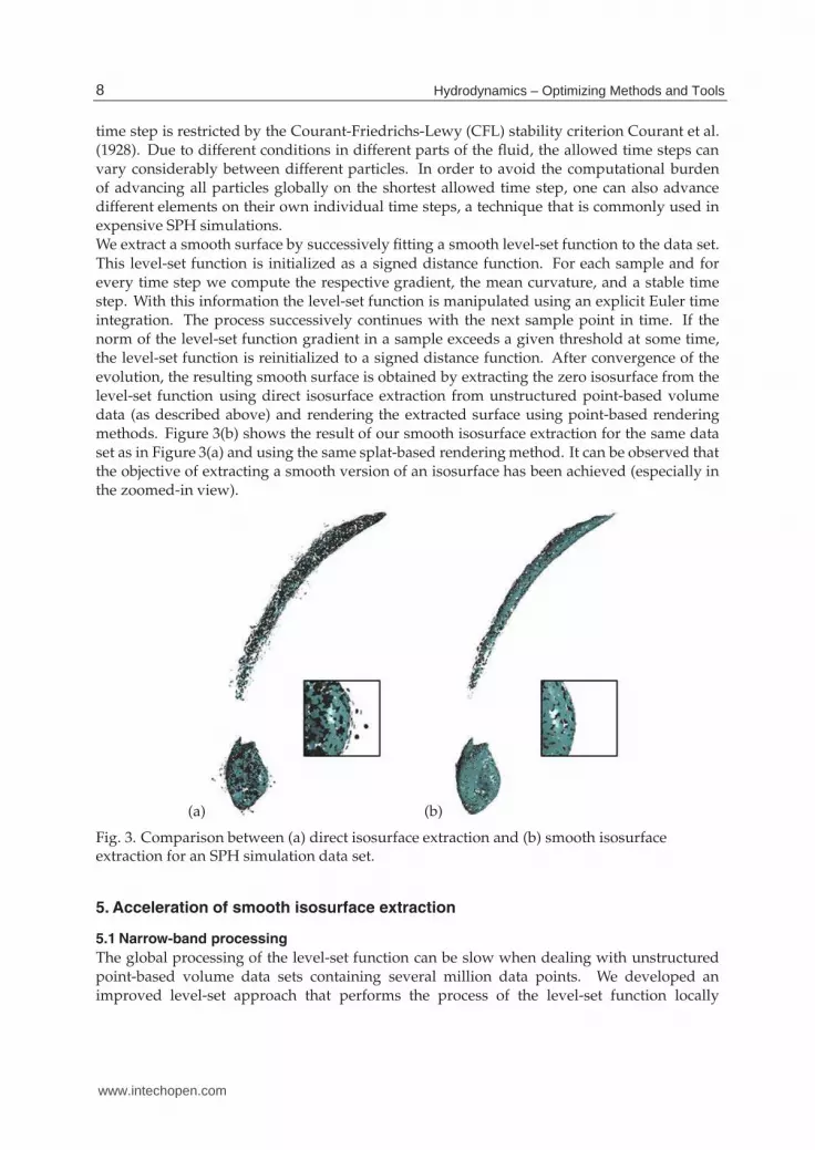
time step is restricted by the Courant-Friedrichs-Lewy (CFL) stability criterion Courant et al.(1928). Due to different conditions in different parts of the fluid, the allowed time steps canvary considerably between different particles. In order to avoid the computational burdenof advancing all particles globally on the shortest allowed time step, one can also advancedifferent elements on their own individual time steps, a technique that is commonly used inexpensive SPH simulations.We extract a smooth surface by successively fitting a smooth level-set function to the data set.This level-set function is initialized as a signed distance function. For each sample and forevery time step we compute the respective gradient, the mean curvature, and a stable timestep. With this information the level-set function is manipulated using an explicit Euler timeintegration. The process successively continues with the next sample point in time. If thenorm of the level-set function gradient in a sample exceeds a given threshold at some time,the level-set function is reinitialized to a signed distance function. After convergence of theevolution, the resulting smooth surface is obtained by extracting the zero isosurface from thelevel-set function using direct isosurface extraction from unstructured point-based volumedata (as described above) and rendering the extracted surface using point-based renderingmethods. Figure 3(b) shows the result of our smooth isosurface extraction for the same dataset as in Figure 3(a) and using the same splat-based rendering method. It can be observed thatthe objective of extracting a smooth version of an isosurface has been achieved (especially inthe zoomed-in view).

(a) (b)

Fig. 3. Comparison between (a) direct isosurface extraction and (b) smooth isosurfaceextraction for an SPH simulation data set.

5. Acceleration of smooth isosurface extraction

5.1 Narrow-band processing

The global processing of the level-set function can be slow when dealing with unstructuredpoint-based volume data sets containing several million data points. We developed animproved level-set approach that performs the process of the level-set function locally


www.intechopen.com


(Rosenthal et al., 2010). Since for isosurface extraction we are only interested in the zerolevel set, values are only updated in regions close to the zero level set. In each iterationof the level-set process, the zero level set is extracted using direct isosurface extractionfrom unstructured point-based volume data and a narrow band around the zero level setis constructed. The band consists of two parts: an inner and an outer band. The inner bandcontains all data points within a small area around the zero level set. These points are updatedwhen executing the level-set step. The outer band encloses the inner band providing all thoseneighbors of the points of the inner band that are necessary to approximate gradients andmean curvature. As before, neighborhood information is obtained using an efficient kd-treescheme, gradients and mean curvature are estimated using a four-dimensional least-squaresfitting approach.The construction of the two-layer band around the zero level set is shown in Figure 4. The zerolevel set (colored blue) is extracted in form of a point cloud representation. Then, all samplepoints with distance to the zero level set less than a distance dα are marked as belonging tothe inner layer of the band (green). Thereafter, all additional sample points needed for thegradient computations within the level-set process are marked as belonging to the outer layerof the band (red points). All other sample points (grey) are not used for the current level-setstep. The distance dα can be estimated using the CFL condition that bounds the level-set step.

Fig. 4. Narrow-band construction for more efficient level-set processing.

How the level-set function is updated after having executed a level-set iteration on thenarrow band with size dα is shown in Figure 5: Points (green) with minimum distance tothe zero-level-set points (blue) smaller than dα

4 have been in the α-band in the preceding timestep and, thus, their level-set function values have been updated in the level-set iteration step.Points (red) in the outer band or with distance to the zero level set greater than dα

2 might havenot be included in the computations of the last level-set iteration step. We assign their level-setfunction value to the signed distance to the zero-level-set points. For all points in the α-band

with a distance to the zero level set in the range[

dα4 , dα

2

]

, the new level-set function value is

interpolated between the level-set function value from the preceding level-set step and theirsigned distance to the zero-level-set points.


www.intechopen.com


$\fr

$\fr

dα4

dα2

Fig. 5. Narrow-band update during level-set procedure (dα denotes the size of the narrowband).

For performance analysis we applied it to an unstructured point-based volume data set witheight million randomly distributed samples. The data set was generated by resampling theregular Hydrogen data set of size 128 × 128 × 128 to the random points. Illustrations of theevolution process for this data set are shown in Figure 6 (Data set courtesy of Peter Fassbinderand Wolfgang Schweizer, SFB 382 University Tübingen.). For each time step, a splat-basedray tracing of the zero level set is shown on the right-hand side. On the left-hand side, a pointrendering of a slab of the data set is shown illustrating the narrow band. Extracted surfacepoints of the zero level set are colored black, sample points in the α-band are colored green,and sample points in the outer band are colored red. Sample points not belonging to thenarrow band are not rendered.The whole local level-set process for extracting a smooth isosurface from the Hydrogen dataset with eight million sample points and given nearest neighbors needed 24 steps and wasperformed in 6 minutes. For the four million version of the data set, the overall computationtime for the entire level-set approach including pre-computations dropped to 84 seconds.This is a significant speed-up in comparison to the time of 13 minutes needed withoutthe narrow-band processing. Still, it produces equivalent results in terms of quality andcorrectness.

5.2 Variational level-set detection of local isosurfaces

Another acceleration of the level-set approach can be achieved by only operating locally on aregion of interest. We derived a variational formulation for smooth local isosurface extractionusing an implicit surface representation in form of a level-set approach, deploying a movingleast-squares (MLS) approximation, and operating on a kd-tree (Molchanov et al., 2011). Thelocality of our approach has two aspects: First, our algorithm extracts only those componentsof the isosurface, which intersect a subdomain of interest. Second, the action of the mainterm in the governing equation is concentrated near the current isosurface position. Bothaspects reduce the computation times per level-set iteration. As for most level-set methodsa reinitialization procedure is needed, but we also consider a modified algorithm where thisstep is eliminated. The final isosurface is extracted in form of a point cloud representation.


www.intechopen.com


Step 9 Step 15

Step 21 Step 24

Fig. 6. Narrow-band level-set evolution.

We also presented a novel point completion scheme that allows us to handle highly adaptivepoint sample distributions.A variational approach is used to derive the local level-set updates. We start with aconstruction of an error functional E, which is the target function that we want to minimize.The error depends on the given data f , the constant fiso representing the isovalue, and alevel-set function ϕ together with its derivatives of first order, i.e., E = E(ϕ,∇ϕ; f , fiso). Thetotal error consists of two weighted terms

E = E1 + λE2, (3)

measuring accuracy and smoothness of the solution, respectively. We propose to use

E1 =14

∫

D(sgn(ϕ(x))− sgn( f (x)− fiso))

2 dx, (4)

andE2 =

∫

Dδ(ϕ(x)) |∇ϕ(x)|dx. (5)

Here, we use the standard definitions of the sign function sgn(x) and the Dirac function δ(x)and the derivative is used in the sense of distributions.A function ϕ∞ minimizing some functional of the form

∫

L(ϕ,∇ϕ)dx should satisfy theEuler-Lagrange equation

(

∂L

∂ϕ− ∑

i

∂

∂xi

∂L

∂ϕi

)

∣

∣

∣

∣

ϕ=ϕ∞

= 0, (6)


www.intechopen.com


where ϕi is the i-th component of ∇ϕ. We derive the Euler-Lagrange equations for functionalsE1 and E2. The idea of a level-set approach is to detect ϕ∞ as a fixed point of an evolutionequation for ϕ = ϕ(x, t) minimizing E. Here, t is an artificial time parameterizing theminimization process ϕ(x, t) → ϕ∞(x) as t → ∞. To construct the PDE, one equates theleft-hand side of Euler-Lagrange Equation with −∂ϕ/∂t. For the functional E, it reads

∂ϕ

∂t= δ(ϕ) (sgn( f − fiso)− sgn(ϕ)) + λ δ(ϕ) ∇ ·

(

∇ϕ

|∇ϕ|

)

. (7)

Subsequently, this equation is regularized and discretized in space and time leading to aniterative process for the value of ϕ at each sample point. Using an explicit Euler timeintegration, we obtain the iteration step

ϕk+1 = ϕk + Δt

[

δǫ(ϕk) (sgn( f − fiso)− sgnǫ(ϕk)) + λ δǫ′ (ϕk) ∇ ·

(

∇ϕk

|∇ϕk|

)]

(8)

which is applied to all sample points xi, where the upper index k stands for the k-th layerin time. This update rule can be applied locally. Figure 7 shows how smooth isosurfacecomponents are extracted locally within a given region of interest.

(a) (b) (c)

Fig. 7. Local level-set evolution of isosurfaces within a region of interest for multi-componentdata sets: (a) selecting region of interest; (b) extracted isosurface components; (c) sameprocedure applied to extract one component of an isosurface from the density field of an SPHsimulation of a white dwarf.

5.3 Non-iterative second-order approximation of signed distance function

Signed distance functions are an obligatory ingredient to the level-set methods. Whenassuming that the underlying function is a signed distance function, several simplificationsand speed-ups of the level set approach can be achieved. Usual approaches for theconstruction of signed distance functions to a surface are either based on iterative solutions ofa special partial differential equation or on marching algorithms involving a polygonizationof the surface. We propose a novel method for a non-iterative approximation of a signeddistance function and its derivatives in a vicinity of a manifold. We use a second-order schemeto ensure higher accuracy of the approximation (Molchanov et al., 2010).The manifold is defined (explicitly or implicitly) as an isosurface of a given scalar field, whichmay be sampled at a set of irregular and unstructured points. We use a spatial subdivision inform of a fast kd-tree implementation to access the samples and perform transformations on


www.intechopen.com


the data. We derive a novel moving least-squares (MLS) approach for a second-order algebraicfitting to locally reconstruct the isosurface. Stability and reliability of the algorithm is achievedby a proper scaling of the MLS weights, accurate choices of neighbors, and appropriatehandling of degenerate cases. We obtain the solution in an explicit form, such that no iterativesolving is necessary, which makes our approach fast. The accuracy relies on second-orderalgebraic fitting.We propose to perform the following steps to construct a signed distance field around animplicitly given isosurface:

1. Given a scalar field f (x) on samples xi, extract a set of isopoints pj corresponding to theisovalue fiso; estimate normals on isopoints nj using kd-tree and MLS technique. Skip thisstep if the isosurface is given explicitly.

2. For a given α > 0 mark all samples xi lying in α-neighborhood of the isosurface; jointlyestablish lists of neighboring isopoints for the marked samples.

3. For each sample yk in the band find its neighbors and check two angles to detect a layersheet.

4. If the sample lies between isosurface components, compute the distances to both of themas in the next step, compare the values found and take the minimal one.

5. If the criterion for a layer is not fulfilled:• perform a local sphere fitting to reconstruct a part of the isosurface close to yk,• if the sphere degenerates to a plane, compute a distance between the sample and the

surface (taking into consideration its orientation),• if the sphere is not degenerated, use the isopoint normals to analyse its convexity and

compute the distance between the sample and the sphere.

An accurate computation of the distance between a sample and an isosurface is hard if theisosurface is represented as a sparse set of isopoints. Therefore a (local) reconstruction ofthe smooth surface is required. In our approach we find an implicit algebraic surface to fitthe discrete data which includes isopoints positions and associated normals. We consideralgebraic spheres of the form

s(x) = a0 + a · x + a4x · x, (9)

where a = (a1, a2, a3) and x = (x1, x2, x3). The solution may naturally degenerate to a plane asa4 vanishes and therefore is exact for flat surfaces. However, a direct enrichment of the class isproblematic: there exist no analytic formula for distance to algebraic ellipsoids. We utilize anapproach of algebraic sphere fitting using positional and derivative constraints. First, we findm + 1 isopoints nearest to the point of interest y. Let h be the distance from y to the farthestneighbor. This parameter will define the support size of the weighting function

ωy(p) = max

{

(

1 −‖y − p‖2

h2

)4

, 0

}

. (10)

Now we look for the optimal algebraic sphere, whose zero-isosurface {x ∈ R3 : s(x) = 0}

optimally fits the positions of the isopoints, i.e., s(pj) = 0, and their normals, i.e., ∇s(pj) = nj.The best fit is defined by parameters a0, . . . , a4 minimizing the cost function

E(a0, . . . , a4) =m

∑j=1

ωj

[

|s(pj)|2 + β‖∇s(pj)− nj‖

2]

(11)


www.intechopen.com


with ωj = ωy(pj). The minimization problem

sopt(x; a0, . . . , a4) = arg min E (12)

has the following explicit solution

a4 =β

2∑ ωjpj · nj − ∑ ωjpj · ∑ ωjnj/Ω

∑ ωjpj · pj − ∑ ωjpj · ∑ ωjpj/Ω, (13)

a = ∑ ωjnj/Ω − 2a4 ∑ ωjpj/Ω, (14)

a0 = a · ∑ ωjpj/Ω − a4 ∑ ωjpj · pj/Ω, (15)

where Ω = ∑ ωj.Figure 8 shows the result when extracting different isosurfaces from a signed distance fieldto a surface in explicit point cloud representation. Isosurfaces for different isovalues fiso ofthe signed distance function field constructed for the bunny data set with 35k surface points,(Data set courtesy of the Stanford University Computer Graphics Laboratory.).

fiso = 4.0 fiso = 2.0 fiso = 0.0 fiso = −3.5

Fig. 8. Isosurfaces extracted from a non-iterative second-order approximation of the signeddistance function to a surface in point cloud representation.

We proposed a novel method for the efficient computation of a signed distance functionto a surface in point cloud representation. This allows us to develop a fast level-setapproach for extracting smooth isosurfaces from point-based volume data, as we can useany point cloud surface as initial zero level set. Since for most applications a roughestimate of the desired surface can be obtained quickly, the overall level-set process canbe shortened significantly. Additionally, we can avoid the computational overhead andnumerical difficulties of PDE-based reinitialization.In summary, putting all acceleration methods together we achieved to reduce the computationcosts for the entire level-set approach including all components by about two orders ofmagnitude. For data sets with 16 million particles, the processing time dropped from tenthsof minutes to tenths of seconds.

6. Image-space point cloud surface rendering

The extracted surfaces are given in point cloud surface representation, i.e., points on thesurfaces with no structure or neighborhood known. Reconstructing a triangular mesh from


www.intechopen.com


these point clouds can be very time consuming. Instead, point-based rendering approacheshave gained a major interest in recent years, basically replacing global surface reconstructionwith local surface estimations using, for example, splats or implicit functions. Crucial totheir performance in terms of rendering quality and speed is the representation of the localsurface patches. We presented a novel approach that goes back to the original ideas ofGrossman & Dally (1998) to avoid any object-space operations and compute high-qualityrenderings by only applying image-space operations (Rosenthal & Linsen, 2008a).Starting from a point cloud including normals (obtained from gradients of the underlyingscalar field), we render a lit point cloud to a texture with color, depth, and normal information.Subsequently, we apply several filter operations. In a first step, we use a mask to fillbackground pixels with the color and normal of the adjacent pixel with smallest depth.The mask assures that only the desired pixels are filled. We use the eight masks shown inFigure 9, where the white pixels indicate background pixels and the dark pixels could be bothbackground or non-background pixels. For each background pixel, we test whether the 3 × 3neighborhood of that pixel matches any of the cases. In case it does, the pixel is not filled.Otherwise, it is filled with the color and depth information of the pixel with smallest depthout of the 3 × 3 neighborhood.

Fig. 9. Filters with size 3 × 3 for detecting whether a background pixel is beyond theprojected silhouette of the object. If one of the eight masks matches the neighborhood of abackground fragment, it is not filled. White cells indicate background pixels, dark cells maybe background or non-background pixels.

Similarly, in a second pass, we fill the pixels that display occluded surface parts. The resultingpiecewise constant surface representation does not exhibit holes anymore and is smoothedby a standard smoothing filter in a third step. The same three steps can also be applied tothe depth channel and the normal map such that a subsequent edge detection and curvaturefiltering leads to a texture that exhibits silhouettes and feature lines. Anti-aliasing along thesilhouettes and feature lines can be obtained by blending the textures. When highlightingthe silhouette and feature lines during blending, one obtains illustrative renderings of the3D objects. The GPU implementation of our approach achieves interactive rates for pointcloud renderings without any pre-computation. Figure 10 shows the individual steps of theproposed pipeline including illustrative rendering. Figure 13(a) shows such another renderingresult for a data set with 883k surface points. The rendering is performed at 52 frames persecond (fps).For a realistic visualization of the models, transparency and shadows are essential features.We propose extensions to our method for point cloud rendering with transparency andshadows at interactive rates (Dobrev et al., 2010a;b). Again, our approach does not requireany global or local surface reconstruction method, but operates directly on the point cloud.All passes are executed in image space and no pre-computation steps are required. The


www.intechopen.com


(a) (b) (c)

(d) (e) (f)

Fig. 10. Image-space point cloud surface rendering pipeline applied to the Dragon data set(Data set courtesy of Stanford University Computer Graphics Lab.): (a) Lit points; (b) afterfilling background pixel; (c) after filling occluded pixels; (d) after smoothing; (e) extractedfeature lines; (f) illustrative rendering.

underlying technique for our approach is a depth peeling method for point cloud surfacerepresentations. The idea of depth peeling is to successively remove the front layer to extracthidden layers. Hence, one virtually renders the object and all visible parts represent the firstlayer. This is removed and the process is iterated to successively extract all hidden layers. Forsurfaces in point cloud representation, another challenge arises, as shown in Figure 11. Whenprojecting the first layer (blue) in point cloud representation to the screen, the layer exhibitsholes such that hidden layers (red) or the background (grey) become visible. To overcomethe problem we use, again, the image-space masks presented above to produce layers withoutholes. Figure 12 shows four different layers of the Blade data set that are extracted using depthpeeling.

Fig. 11. Depth peeling for point cloud surfaces.

Having detected a sorted sequence of surface layers, they can be blended front to back withgiven opacity values to obtain renderings with transparency. These computation steps achieveinteractive frame rates. Figure 13(b) shows a rendering with transparency. The rendering isperformed at 17.5 fps.To determine which parts of a surface are directly lit by a light source and which parts fall intothe shadow of the light source, we determine and mark all points that are visible from the light


www.intechopen.com


(a) (b) (c) (d)

Fig. 12. Four successive layers extracted using depth peeling on point cloud surfacerepresentations.

source similar to “pre-baking” irradiance textures for polygonal mesh scenes. We use pointcloud shadow textures, which are basically Boolean arrays that store which points are lit. Oncethe shadow texture is determined, lit points are drawn properly illuminated with ambient,diffuse, and specular reflection components using Phong’s illumination model (Phong, 1975),while unlit points are only drawn using the ambient reflection component. This illuminationcreates the effect of shadows, as only those points are marked unlit where the light source isoccluded by other surface parts.To determine which points are visible from the light source, we render the scene with thelight source’s position being the viewpoint with depth testing enabled. All visible points aremarked in an array. However, we observe that, due to the high point density, it is not unusualthat several adjacent points of one surface layer project to the same fragment position. Thesuggested procedure would only mark the closest point for each fragment as lit, which wouldlead to an inconsistent shadow textures. Again, depth peeling is the key to solve this problem,but we apply it differently. While for transparent surface rendering our goal was to extractdifferent surface layers, now we use it to find all the points that belong to a single surfacelayer, namely the closest one.For the shadow texture computation, we also apply a Monte-Carlo integration method toapproximate light from an area light source, leading to soft shadows. Shadow computationsfor point light sources are executed at interactive frame rates. Shadow computations for arealight sources are performed at interactive or near-interactive frame rates depending on theapproximation quality. Figure 13(c) shows a rendering with shadows using the Monte-Carloapproach. The rendering with 5 Monte Carlo samples is performed at 9 fps, while therendering without Monte-Carlo sampling, i.e., with 1 sample, is performed at 25 fps.

(a) (b) (c)

Fig. 13. (a) Image-space point cloud surface rendering applied to the Blade data set (courtesyof Visualization Toolkit). (b) Rendering with transparency using depth-peeling approach. (c)Rendering with shadows using Monte-Carlo integration.


www.intechopen.com


We also investigated the use of ray tracing techniques for high-quality rendering based onsplat representations, but the complexity of this approach impedes interactivity (Linsen et al.,2007).

7. Surface extraction from multiple fields

As the data sets resulting from SPH simulations typically contain a multitude of physicalvariables, it is desirable that visualization methods take into account the entire multi-fieldvolume data rather than concentrating on one variable. We presented a visualization approachbased on surface extraction from multi-field particle volume data (Linsen et al., 2008). Thesurfaces segment the data with respect to the underlying multi-variate function. Decisionson segmentation properties are based on the analysis of the multi-dimensional attributespace. The attribute space exploration is performed by an automated multi-dimensionalhierarchical clustering method, whose resulting density clusters are shown in the form ofdensity level sets in a 3D star coordinate layout (Long, 2010; Long & Linsen, 2011). In the starcoordinate layout, the user can select clusters of interest. A selected cluster in attribute spacecorresponds to a segmenting surface in object space. Based on the segmentation propertyinduced by the cluster membership, we extract a surface from the volume data. We directlyextract our surfaces from the SPH data without prior resampling or grid generation. Thesurface extraction computes individual points on the surface, which is supported by anefficient neighborhood computation. The extracted surface points are, again, rendered usingpoint-based rendering operations. Our approach combines methods in scientific visualizationfor object-space operations with methods in information visualization for attribute-spaceoperations.

7.1 Attribute space visualization

Given the multi-dimensional attribute space with a large number of d-dimensional pointslying in that attribute space, each point corresponds to one sample of the volumetric data fieldand each dimension represents one data attribute (typically one scalar value) stored at thatsample. In order to understand the distribution of the points in attribute space, we propose tocompute a density function and to determine the number of clusters as well as the high densityregion of each cluster. Given a multivariate density function f (x) in d dimensions, modes off (x) are positions where f (x) has local maxima. Thus, a mode of a given distribution is moredense than its surrounding area. We want to find the attraction regions of modes. To doso, we choose various values for constants λ (0 < λ < supx f (x)) and consider regions ofthe particle space where values of f (x) are greater than or equal to λ. The λ-level set of thedensity function f (x) denotes a set S( f , λ) = {x ∈ R

d : f (x) ≥ λ} . The set S( f , λ) consists ofa number q of connected components Si( f , λ) that are pairwise disjoint. The subsets Si( f , λ)are called λ-density clusters (λ-clusters for short). A cluster can contain one or more modesof the respective density function. Let the domain of the data set be given in the form of ad-dimensional hypercube, i. e., a d-dimensional bounding box. To derive the density function,we spatially subdivide the domain of the data set into cells of equal shape and size. Thus,the spatial subdivision provides a binning into d-dimensional cells. For each cell we count thenumber of points lying inside. The multivariate density function f (x) is given by the numberof points per cell divided by the cell’s area and the overall number of data points. As thearea is equal for all cells, the density of each cell is proportional to the number of data pointslying inside the cell. The cell should be small enough such that local changes of the density


www.intechopen.com


function can be detected but also large enough to contain a large number of points such thataveraging among points is effective. Because of the curse of dimensionality, there will be manyempty cells. We do not need to store empty cells such that the amount of cells we are storingand dealing with is (significantly) smaller than the number of the d-dimensional points. Theλ-clusters can be computed by detecting regions of connected cells with densities larger thanλ. As we identify density with point counts, the densities are integer values. Hence, we startby computing density clusters for λ = 1. Subsequently, we process each detected λ-clusterindividually by iteratively removing those cells with minimum density, where the minimumdensity increases in steps of 1. If this process causes a cluster to fall into two subclusters,the subclusters represent higher-density clusters within the original cluster. If a cluster doesnot fall into subclusters during the process, it is a mode cluster. This process generates ahierarchical structure, which is summarized by the high density cluster tree (short: clustertree). The root of the cluster tree represents all points. Figure 14(a) shows a cluster tree with4 mode clusters represented by the tree’s leaves. Cluster tree visualization provides a methodto understand the distribution of data by displaying the attraction regions of modes of themultivariate density function. Each cluster contains at least one mode.

(a) (b) (c)

Fig. 14. (a) Cluster tree of density visualization with four modes shown as leaves of the tree.(b) Nested density cluster visualization based on cluster tree using 3D star coordinates. (c)Right-most cluster in (b) is selected and its homogeneity is evaluated using parallelcoordinates.

Having computed the d-dimensional high density clusters, we need to project them into athree-dimensional space for visualization purposes. In order to visualize the high densityclusters in a way that allows clusters to be correlated with the d dimensions, we need to usea coordinate system that incorporates all d dimensions. Such a coordinate system can beobtained by using star coordinates. When projecting the d-dimensional high density clustersinto a three-dimensional star coordinate representation, clusters should remain clusters. Thus,points that are close to each other in the d-dimensional feature space should not be furtherapart after projection into the three-dimensional space. Let O be the origin of the 3D starcoordinate system and (a1, . . . , ad) be a sequence of d three-dimensional vectors representingthe axes. The mapping of a d-dimensional data point x = (x1, . . . , xd) to a three-dimensionaldata point Π(x) is determined by the average sum of vectors ak of the 3D star coordinatesystem multiplied with its attributes xk for k = 1, . . . , d, i.e.,

Π(x) = O +1d

d

∑k=1

xkak. (16)


www.intechopen.com


Since it can be shown that||Π(x)− Π(y)||1 ≤ ||x − y||1 (17)

for any d-dimensional points x and y, the distance of the images of two d-dimensional pointsis lower than or equal to the distance of the points with respect to the L1-norm. Therefore,two points in the multi-dimensional space are projected to 3D star coordinates preserving thesimilarity properties of clusters (at least with respect to the L1-norm). In other words, themapping of d-dimensional data to the 3D visual space does not break clusters. The secondproperty that our projection from multi-dimensional feature space into three-dimensionalstar coordinate systems should fulfill is that separated clusters should not be projected intothe same region. The projection into star coordinates may cause severe cluttering of clusterswhen not carefully choosing the axes (a1, . . . , ad). To alleviate the problem of overlappingclusters we introduce a method which chooses a "good" coordinate system. Assume that ahierarchy of high density clusters have q mode clusters, which do not contain any higher leveldensities. Let mi be the barycenter of the points within the ith cluster, i = 1, . . . , q. We want tochoose a projection that maintains best the distances between clusters. Let {v1, v2, v3} be anorthonormal basis of the candidate three-dimensional space of projections. The desired choiceof a 3D star coordinate layout is to maximize the distance of the q projected barycenters VTmi

with V = [v1, v2, v3]T, i.e. to maximize the objective function

∑i<j

||VTmi − VTmj||2 = trace(VTSV) (18)

withS = ∑

i<j

(mi − mj)(mi − mj)T . (19)

Thus, the three vectors v1, v2, v3 are the three unit eigenvectors corresponding to the threelargest eigenvalues of matrix S. This step is a principal component analysis (PCA) applied tothe barycenters of the clusters. As a result, we choose the d three-dimensional axes of the 3Dstar coordinate system as ai = (v1i, v2i, v3i), i = 1, . . . , d.Obviously, we can also project into 2D coordinates in the same way. However, whencomparing and evaluating projections to 2D and 3D visual space (Poco et al., 2011), aquantitative analysis confirms that 3D projections outperform 2D projections in terms ofprecision. Moreover, a user study indicates that certain tasks can be more reliably andconfidently answered with 3D projections. Nonetheless, as 3D projections are displayed on2D screens, interaction is more difficult.After having computed the projected clusters, we can display them using star coordinates byrendering a point primitive for each projected data point. A less cluttered and more beautifuldisplay is to render the boundary of the clusters. Considering the cluster that is described bythe set of points {pi = (xi, yi, zi) : i = 1, . . . , m} after being projected into the 3D space.In order to compute the boundary of this group of points,we need to have a continuousrepresentation of the group. Therefore, we consider the function

fh(p) =m

∑i=1

K

(

p − pi

h

)

, p ∈ R3 , (20)

where K is a kernel function and h is the bandwidth. Then, we can reconstruct the field over aregular grid and render the boundary set of the points by using standard isosurface extraction


www.intechopen.com


methods to extract the boundary surface of the set S(h, c) = {p ∈ R3 : fh(p) ≥ c}, where c

is an isovalue. We choose parameter h and c to guarantee that S(h, c) is connected and has avolume of minimum extension. The kernel function should be sufficiently smooth and havea small compact support. For example, we can choose K(p) = (1 − ||p||2)2 for ||p|| ≤ 1 andK(p) = 0 otherwise and the bandwidth h to be equal to the longest length of the minimumspanning tree of these m points. In Figure 14(b) we show the visualization of the clusters byrendering such boundary surfaces, where it can be shown that for the chosen kernel isovaluec = 9

16 is appropriate. In order to visualize all clusters of the cluster tree, we render thesurfaces in a semi-transparent fashion. The resulting visualization shows sequences of nestedsurfaces, where the inner surfaces represent higher density levels. Figure 14(b) shows thenested density cluster visualization with respect to the cluster tree in Figure 14(a).

7.2 Coordinated views

Generating all clusters and displaying them in star coordinates allows for further analysisof the detected clusters. The simplest interaction method is to select individual clusters byjust clicking at the boundary surface. When a cluster is selected, intra-cluster variability isvisualized using parallel coordinates, see Figure 14(b) and (c). In both pictures the relationbetween the selected cluster with the dimension can be observed.Moreover, we visualize the coordinated view in physical space, which exhibits the spatiallocation of the selected feature. The rendering in physical space can be preformed by justplotting all particles that belong to the selected feature or by extracting a boundary surfaceof that feature, i.e., a surface that separates all particles that belong to the feature from allparticles that do not belong to the feature. Figure 15 shows an attribute-space rendering of thedetected clusters in 3D optimized star coordinates (a), a color-coded object-space renderingof the clustered particles (b), and a separation surface of clusters in object space (c). Theunderlying SPH simulation is that of tidal disruption and ignition of a white dwarf by amoderately massive black hole (Rosswog et al., 2009).

(a) (b) (c)

Fig. 15. (a) Seven-dimensional attribute space visualization of SPH data set using optimized3D star coordinates. (b) Object space visualization of cluster distribution. (c) Object spacevisualization of a separating surface.

For the visualization of enclosing surfaces in attribute as well as in object space, we lookedinto an alternative approach of enclosing surfaces for point clusters using 3D discrete Voronoidiagrams (Rosenthal & Linsen, 2009). Our system provides three different types of enclosingsurfaces. By generating a discrete distance field to the point cluster and extracting anisosurface from the field, an enclosing surface with any distance to the point cluster can be


www.intechopen.com


generated. As a second type of enclosing surfaces, a hull of the point cluster is extracted. Thegeneration of the hull uses a projection of the discrete Voronoi diagram of the point clusterto an isosurface to generate a polygonal surface. Generated hulls of non-convex clusters arealso non-convex. The third type of enclosing surfaces can be created by computing a distancefield to the hull and extracting an isosurface from the distance field. This method exhibitsreduced bumpiness and can extract surfaces arbitrarily close to the point cluster withoutlosing connectedness. Figure 16 shows the idea of the different approaches starting froman isosurface from the distance field to the point cluster (a), connecting the neighbors thatcontribute to the surface in (a) to form a non-convex hull (b), and computing surfaces thatare equidistant to the computed non-convex hull (b). Figure 17 shows a comparison of thedifferent enclosing surfaces when applied to a cluster of points when projected into optimizedstar coordinates.

a) b)

Fig. 16. (a) Extracting an isosurface from the distance field to the point cluster. Voronoiregions on the isosurface induce neighborhoods. (b) Neighbors are connected to form a hull.The image also shows an isosurface extracted from the distance field to the hull.

We extended our work on interactivity by explicitly encoding the cluster hierarchy in atree that is visually encoded in a radial layout. Coordinated views between cluster treevisualization and parallel coordinates as well as object-space visualizations allow for aninteractive analysis of multi-field SPH data (Linsen et al., 2009). The cluster tree allows for theselection of detected clusters, the parallel coordinate plots show the properties of the selectedclusters, and object-space visualizations in form of extracted surfaces or particle distributionsexhibit the location of the respective clusters in physical space. Figure 18 shows such a visualanalysis set-up when applied to the IEEE Visualization Contest data (Rosenthal et al., 2008).We also proposed a method to integrate the parallel coordinates into the cluster treevisualization. The MultiClusterTree approach (Long & Linsen, 2011) uses circular parallelcoordinates for the embedding into the radial hierarchical cluster tree layout, which allowsfor the analysis of the overall cluster distribution. This visual representation supports thecomprehension of the relations between clusters and the original attributes. The combinationof the 2D radial layout and the circular parallel coordinates is used to overcome theoverplotting problem of parallel coordinates when looking into data sets with many records.Figure 19 shows how integrated circular coordinates can provide a good overview of thecluster distribution.


www.intechopen.com


Fig. 17. Different visualizations of two point clusters (colored red and blue) from the 2008IEEE Visualization Design Contest data. The clusters were found using density-basedclustering of multidimensional feature space and were projected to a 3D visual space using alinear projection. Additionally to the cluster points (a), three types of enclosing surfaces areshown. (b) Isosurface extraction from distance field computed using a 3D discrete Voronoidiagram of resolution 256 × 256 × 256. (c) Hull of the cluster computed from the isosurfaceof the distance field. (d) Isosurface extraction from distance field to hull.

Fig. 18. Coordinated views allow for selecting clusters in cluster tree and investigatingproperties in attribute space (using parallel coordinates) as well as locations in physicalspace.

8. Interactive visual system for exploration of multiple scalar and flow fields

Our research results are combined in the SmoothViz software system that is offered to the SPHcommunity via our website (http://vcgl.jacobs-university.de/software). Not all presentedfeatures are included yet. Currently, the system consists of three modules responsible


www.intechopen.com


Fig. 19. Integrated circular parallel coordinates in clusters tree visualization for data set withhierarchical clusters.

for time-varying data manipulation, scalar field exploration, and flow field visualization.An intuitive graphical user interface (GUI) allows for easy processing and interaction.Additional functionalities and visualizations that are common in the SPH community havebeen included.First, the user can load SPH data containing time-varying particle positions and time-varyingmultiple scalar and vector field values sampled at the particles. A 3D view of the particledistribution at a chosen time step allows the user to adjust the viewing parameters usingarbitrary rotation and translation of camera. Loading of successive or preceding time stepsfrom the time-varying series of data sets is as easy as play or rewind in a standard mediaplayer. Extracted pathlines can show evolution in time of an individual particle or sets ofparticles. Figure 20(a) shows the GUI and a particle distribution plot for a chosen time step.There are two options to represent the structure of a selected scalar field: Maximal intensityprojection plots can render any of the scalar fields using one of the build-in color maps andallowing for manually modifying the transfer function. Figure 20(b) shows the GUI for thetransfer function modification and the respective maximum intensity plot of a chosen scalarfield. Alternatively, isosurfaces can be extracted for interactively selected isovalues and shownusing a point splatting technique or a dense point cloud rendering. Figure 20(c) shows anumber of nested isosurfaces using point cloud renderings.Finally, a specified number of streamlines can be computed with respect to the vector fieldchosen by the user. Combined views are possible to explore multiple fields simultaneously,e.g. multiple isosurfaces together with stream- or pathlines. Figure 20(d) shows an isosurfacerendering using point splatting combined with a rendering of selected streamlines. For moredetails on the system, we refer to the user manual that comes with the SmoothViz softwarepackage.


www.intechopen.com


(a) (b)

(c) (d)

Fig. 20. Screenshots of SmoothViz software system for SPH data exploration: (a)Three-dimensional particle distribution modeling a White Dwarf passing close to a BlackHole. (b) Maximal intensity projection plot of the density field of a White Dwarf with userdefined transfer function; (c) Several density isosurfaces of two White Dwarfs in point-basedrepresentation. (d) Interplay of a velocity field (shown with streamlines) and a temperaturefield (shown as splatted isosurface).

9. Conclusion

We have presented approaches for visualization of SPH data. All methods operate directlyon the particles that are distributed in a highly adaptive and irregular manner and that donot have any connectivity. Operating on the particles avoids the introduction of errors thatoccur when resampling to a grid. Our visualizations focus on surface extractions from suchdata. We first presented an isosurface extraction from any scalar field of the SPH data. Itexploits a fast navigation through a kd-tree via an indexing structure and allows for fastisosurface extraction of high quality. Because of approximations made during simulation, itis desirable to add a smoothing term to the isosurface extraction method. This is achievedby the use of level-set methods. Again, the method operates on the particles only. Wehave presented several ways on how to accelerate the computations including a narrow-bandapproach, a local variational approach, and a signed distance function computation to anyisosurface representation. Extracted isosurfaces are given in form of point clouds. Wepresented how they can be rendered using an image-space point cloud rendering approachthat avoids any pre-computation and thus can immediately applied to any extracted surface.Shadows and transparency are supported at interactive rates. We further extended thework to the extraction of boundary surfaces of features in multi-field data. The attributespace of the multi-field data is being explored using clustering and cluster visualization


www.intechopen.com


methods. Coordinated or integrated views to parallel or circular coordinates, respectively,allow for further visual analysis of the properties of the extracted clusters. Coordinated viewsto object space allow for the investigation of the spatial distribution of detected features.Enclosing surfaces show the cluster boundaries. The presented functionality has partiallybeen incorporated into the SmoothViz software package including further features such asgeometric flow visualization. It allows for interactive exploration and integrated analysis ofmultiple fields of SPH data.

10. Acknowledgments

This work was supported by the German Research Foundation (DFG) under grant number LI1530/6-1.

11. References

Biddiscombe, J., Graham, D. & Maruzewski, P. (2008). Visualization and analysis of SPH data,ERCOFTAC Bulletin 76(9-12).

Borouchaki, H., Hecht, F., Saltel, E. & George, P. (1995). Reasonably efficient delaunaybased mesh generator in 3 dimensions, 4th International Meshing Roundtable, SandiaNational Laboratories, pp. 3–14.

CGAL (2011). Computational geometry algorithms library (CGAL), http://www.cgal.org/.Cha, D., Son, S. & Ihm, I. (2009). Gpu-assisted high quality particle rendering, Computer

Graphics Forum 28(4): 1247–1255.Co, C. S. & Joy, K. I. (2005). Isosurface Generation for Large-Scale Scattered Data Visualization,

in G. Greiner, J. Hornegger, H. Niemann & M. Stamminger (eds), Proceedingsof Vision, Modeling, and Visualization 2005, Akademische Verlagsgesellschaft AkaGmbH, pp. 233–240.

Courant, R., Friedrichs, K. & Lewy, H. (1928). Über die partiellen differenzengleichungen dermathematischen physik, Mathematische Annalen 100(1): 32 – 74.

Delaunay, B. N. (1934). Sur la sphere vide, Bull. Acad. Sci. USSR 7: 793–800.Dobrev, P., Rosenthal, P. & Linsen, L. (2010a). An image-space approach to interactive

point cloud rendering including shadows and transparency, Computer Graphics andGeometry 12(3): 2–25.

Dobrev, P., Rosenthal, P. & Linsen, L. (2010b). Interactive image-space point cloud renderingwith transparency and shadows, in V. Skala (ed.), Communication Papers Proceedingsof WSCG, The 18th International Conference on Computer Graphics, Visualization andComputer Vision, UNION Agency – Science Press, Plzen, Czech Republic, pp. 101–108.

Du, Q. & Wang, D. (2006). Recent progress in robust and quality delaunay mesh generation,J. Comput. Appl. Math. 195(1): 8–23.

Fraedrich, R., Auer, S. & Westermann, R. (2010). Efficient high-quality volume rendering ofsph data, IEEE Transactions on Visualization and Computer Graphics 16: 1533–1540.

Fraedrich, R., Schneider, J. & Westermann, R. (2009). Exploring the "millennium run" - scalablerendering of large-scale cosmological datasets, IEEE Transactions on Visualization andComputer Graphics 15(6): 1251–1258.

George, P. L., Hecht, F. & Saltel, E. (1991). Automatic mesh generator with specified boundary,Comput. Methods Appl. Mech. Eng. 92(3): 269–288.


www.intechopen.com


Gingold, R. A. & Monaghan, J. J. (1977). Smoothed particle hydrodynamics - Theory andapplication to non-spherical stars, Monthly Notices of the Royal Astronomical Society181: 375–389.

Grossman, J. P. & Dally, W. J. (1998). Point sample rendering, Proceedings of 9th EurographicsWorkshop on Rendering, pp. 181–192.

Hopf, M. & Ertl, T. (2003). Hierarchical splatting of scattered data, Visualization Conference,IEEE .

Hopf, M., Luttenberger, M. & Ertl, T. (2004). Hierarchical splatting of scattered 4d data, IEEEComputer Graphics and Applications 24: 64–72.

Linsen, L., Long, T. V. & Rosenthal, P. (2009). Linking multi-dimensional feature space clustervisualization to surface extraction from multi-field volume data, IEEE ComputerGraphics and Applications 29(3): 85–89.

Linsen, L., Long, T. V., Rosenthal, P. & Rosswog, S. (2008). Surface extraction from multi-fieldparticle volume data using multi-dimensional cluster visualization, IEEE Transactionson Visualization and Computer Graphics 14(6): 1483–1490.

Linsen, L., Müller, K. & Rosenthal, P. (2007). Splat-based ray tracing of point clouds, Journal ofWSCG 15(1–3): 51–58.

Long, T. V. (2010). Visualizing High Density Clusters in Multidimensional Data, PhD thesis, JacobsUniversity.

Long, T. V. & Linsen, L. (2011). Visualizing high density clusters in multidimensional datausing optimized star coordinates, Journal of Computational Statistics (to appear) .

Lucy, L. B. (1977). A numerical approach to the testing of the fission hypothesis, AstronomicalJournal 82: 1013–1024.

Maur, P. & Kolingerová, I. (2001). Post-optimization of delaunay tetrahedrization, SCCG ’01:Proceedings of the 17th Spring conference on Computer graphics, IEEE Computer Society,Washington, DC, USA, p. 31.

Molchanov, V., Rosenthal, P. & Linsen, L. (2010). Non-iterative second-order approximation ofsigned distance function for any isosurface representation, Computer Graphics Forum29(3): 1211–1220.

Molchanov, V., Rosenthal, P. & Linsen, L. (2011). Variational level-set detection of localisosurfaces from unstructured point-based volume data, Schloss Dagstuhl ScientificVisualization Workshop 2009 Follow-up, to appear.

Navratil, P. A., Johnson, J. L. & Bromm, V. (2007). Visualization of cosmological particle-baseddatasets, 13(6): 1712–1718.

Pav, S. E. & Walkington, N. J. (2004). Robust three dimensional delaunay refinement, 13thInternational Meshing Roundtable, Sandia National Laboratories, SAND 2004-3765C,pp. 145–156.

Phong, B. T. (1975). Illumination for computer generated pictures, Commun. ACM 18: 311–317.Poco, J., Etemadpour, R., Paulovich, F. V., Long, T. V., Rosenthal, P., de Oliveira, M. C. F.,

Linsen, L. & Minghim, R. (2011). A framework for exploring multidimensional datawith 3d projections, Computer Graphics Forum 30(3): 1111–1120.

Price, D. (2007). SPLASH: An interactive visualisation tool for smoothed particlehydrodynamics simulations, Publications of the Astronomical Society of Australia24: 159–173.

Rosenberg, I. D. & Birdwell, K. (2008). Real-time particle isosurface extraction, Proceedings ofthe 2008 symposium on Interactive 3D graphics and games, I3D ’08, ACM, New York, NY,USA, pp. 35–43.


www.intechopen.com


Rosenthal, P. (2009). Direct Surface Extraction from Unstructured Point-based Volume Data, ShakerVerlag, Aachen, Germany (Ph.D. Thesis Jacobs University, Bremen, Germany).

Rosenthal, P. & Linsen, L. (2006). Direct isosurface extraction from scattered volume data,in B. S. Santos, T. Ertl & K. I. Joy (eds), Eurographics / IEEE VGTC Symposium onVisualization - EuroVis 2006, pp. 99–106,367.

Rosenthal, P. & Linsen, L. (2008a). Image-space point cloud rendering, Proceedings of ComputerGraphics International, pp. 136–143.

Rosenthal, P. & Linsen, L. (2008b). Smooth surface extraction from unstructured point-basedvolume data using PDEs, IEEE Transactions on Visualization and Computer Graphics14(6): 1531–1546.

Rosenthal, P. & Linsen, L. (2009). Enclosing surfaces for point clusters using 3d discretevoronoi diagrams, Computer Graphics Forum 28(3): 999–1006.

Rosenthal, P., Long, T. V. & Linsen, L. (2008). "Shadow Clustering": Surface extractionfrom non-equidistantly sampled multi-field 3D scalar data using multi-dimensionalcluster visualization, VisWeek 08 Conference Compendium, Winner of IEEEVisualization Design Contest.

Rosenthal, P., Molchanov, V. & Linsen, L. (2010). A narrow band level set method for surfaceextraction from unstructured point-based volume data, in V. Skala (ed.), Proceedingsof WSCG, The 18th International Conference on Computer Graphics, Visualization andComputer Vision, UNION Agency – Science Press, Plzen, Czech Republic, pp. 73–80.

Rosenthal, P., Rosswog, S. & Linsen, L. (2007). Direct surface extraction from smoothedparticle hydrodynamics simulation data, Proceedings of the 4th High-End VisualizationWorkshop, Lehmanns Media - LOB, pp. 50–61.

Rosswog, S. (2009). Astrophysical smooth particle hydrodynamics, New Astronomy Reviews53(4-6): 78 – 104.

Rosswog, S., Ramirez-Ruiz, E. & Hix, W. R. (2009). Tidal Disruption and Ignition of WhiteDwarfs by Moderately Massive Black Holes, Astrophysical Journal 695: 404–419.

Sapidis, N. S. & Perucchio, R. (1991). Domain delaunay tetrahedrization of arbitrarily shapedcurved polyhedra defined in a solid modeling system, SMA ’91: Proceedings of the firstACM symposium on Solid modeling foundations and CAD/CAM applications, ACM Press,New York, NY, USA, pp. 465–480.

Schindler, B., Fuchs, R., Biddiscombe, J. & Peikert, R. (2009). Predictor-corrector schemesfor visualization ofsmoothed particle hydrodynamics data, IEEE Transactions onVisualization and Computer Graphics 15: 1243–1250.

Walker, R., Kenny, P. & Miao, J. (2005). Visualization of Smoothed Particle Hydrodynamicsfor Astrophysics, in L. Lever & M. McDerby (eds), Theory and Practice of ComputerGraphics 2005, Eurographics Association, University of Kent, UK, pp. 133–138.(Electronic version http://diglib.eg.org).URL: http://www.cs.kent.ac.uk/pubs/2005/2230


www.intechopen.com

Hydrodynamics - Optimizing Methods and ToolsEdited by Prof. Harry Schulz

ISBN 978-953-307-712-3Hard cover, 420 pagesPublisher InTechPublished online 26, October, 2011Published in print edition October, 2011

InTech EuropeUniversity Campus STeP Ri Slavka Krautzeka 83/A 51000 Rijeka, Croatia Phone: +385 (51) 770 447 Fax: +385 (51) 686 166www.intechopen.com

InTech ChinaUnit 405, Office Block, Hotel Equatorial Shanghai No.65, Yan An Road (West), Shanghai, 200040, China

Phone: +86-21-62489820 Fax: +86-21-62489821

The constant evolution of the calculation capacity of the modern computers implies in a permanent effort toadjust the existing numerical codes, or to create new codes following new points of view, aiming to adequatelysimulate fluid flows and the related transport of physical properties. Additionally, the continuous improving oflaboratory devices and equipment, which allow to record and measure fluid flows with a higher degree ofdetails, induces to elaborate specific experiments, in order to shed light in unsolved aspects of the phenomenarelated to these flows. This volume presents conclusions about different aspects of calculated and observedflows, discussing the tools used in the analyses. It contains eighteen chapters, organized in four sections: 1)Smoothed Spheres, 2) Models and Codes in Fluid Dynamics, 3) Complex Hydraulic Engineering Applications,4) Hydrodynamics and Heat/Mass Transfer. The chapters present results directed to the optimization of themethods and tools of Hydrodynamics.

How to referenceIn order to correctly reference this scholarly work, feel free to copy and paste the following:

Lars Linsen, Vladimir Molchanov, Petar Dobrev, Stephan Rosswog, Paul Rosenthal and Tran Van Long(2011). SmoothViz: Visualization of Smoothed Particles Hydrodynamics Data, Hydrodynamics - OptimizingMethods and Tools, Prof. Harry Schulz (Ed.), ISBN: 978-953-307-712-3, InTech, Available from:http://www.intechopen.com/books/hydrodynamics-optimizing-methods-and-tools/smoothviz-visualization-of-smoothed-particles-hydrodynamics-data

smoothviz: visualization of smoothed particles hydrodynamics data

Documents