adaptive smoothed aggregation ($\\alpha$sa) multigrid

$: Adaptive Smoothed Aggregation ($\\alpha$SA) Multigrid$
SIAM REVIEW c© 2005 Society for Industrial and Applied MathematicsVol. 47, No. 2, pp. 317–346

Adaptive SmoothedAggregation (αSA) Multigrid∗

M. Brezina†

R. Falgout‡

S. MacLachlan†

T. Manteuffel†

S. McCormick†

J. Ruge†

Abstract. Substantial effort has been focused over the last two decades on developing multileveliterative methods capable of solving the large linear systems encountered in engineeringpractice. These systems often arise from discretizing partial differential equations overunstructured meshes, and the particular parameters or geometry of the physical problembeing discretized may be unavailable to the solver. Algebraic multigrid (AMG) and mul-tilevel domain decomposition methods of algebraic type have been of particular interestin this context because of their promises of optimal performance without the need for ex-plicit knowledge of the problem geometry. These methods construct a hierarchy of coarseproblems based on the linear system itself and on certain assumptions about the smoothcomponents of the error. For smoothed aggregation (SA) multigrid methods applied todiscretizations of elliptic problems, these assumptions typically consist of knowledge of thenear-kernel or near-nullspace of the weak form. This paper introduces an extension of theSA method in which good convergence properties are achieved in situations where explicitknowledge of the near-kernel components is unavailable. This extension is accomplishedin an adaptive process that uses the method itself to determine near-kernel componentsand adjusts the coarsening processes accordingly.

Key words. algebraic multigrid (AMG), generalized smoothed aggregation (SA), adaptive method,black-box method

AMS subject classifications. 65F10, 65N55, 65F30

DOI. 10.1137/050626272

1. Introduction. Increasing demands for accuracy in computational simulationhave led to significant innovation in both computer hardware and algorithms for scien-tific computation. Multigrid methods have demonstrated their efficiency in solving thelinear systems generated by discretizing elliptic partial differential equations (PDEs),including Laplace’s and those of linear elasticity. Algebraic multigrid (AMG) methods

∗Published electronically April 29, 2005. This paper originally appeared in SIAM Journal onScientific Computing, Volume 25, Number 6, 2004, pages 1896–1920. This work was sponsored bythe Department of Energy under grants DE-FC02-01ER25479 and DE-FG03-99ER25217, LawrenceLivermore National Laboratory under contract B533502, Sandia National Laboratories under con-tract 15268, and the National Science Foundation under grant DMS-0410318.

http://www.siam.org/journals/sirev/47-2/62627.html†Department of Applied Mathematics, Campus Box 526, University of Colorado at Boulder,

Boulder, CO 80309-0526 ([email protected], [email protected], [email protected], [email protected], [email protected]).‡Center for Applied Scientific Computation, Lawrence Livermore National Lab, P.O. Box 808,

Livermore, CA 94551 ([email protected]).

317

318 BREZINA ET AL.

offer this efficiency without reliance on knowledge of the grid geometry or of variationin the coefficients of the differential operator. For these reasons, AMG algorithms areoften the method of choice for solving linear systems that arise from discretizationsover unstructured grids or with significant variation in the operator.

Over the last decade, smoothed aggregation (SA; cf. [21, 23, 22, 20, 9]) hasemerged as an efficient AMG solver for the algebraic systems obtained by discretizingcertain classes of differential equations on unstructured meshes. In particular, SA is of-ten very efficient at solving the systems that arise from problems of three-dimensional(3D) thin-body elasticity, a task that can tax traditional AMG techniques.

As with classical AMG [4, 18, 19], the standard SA method bases its transferoperators on certain assumptions about the nature of algebraically smooth error, thatis, error that simple relaxation schemes, such as Jacobi or Gauss–Seidel, cannot effec-tively eliminate. For SA applied to discretizations of elliptic PDEs, this assumptionusually takes the form of explicit knowledge of the near-kernel of the associated weakform. This knowledge is easy to obtain for large classes of problems. For example, itis simple to determine representative near-kernel components for finite element dis-cretizations of second- or fourth-order PDEs, including many nonscalar problems. Inmore general situations, however, this knowledge may not be readily available.

Consider the case where a matrix is provided without knowledge of how the orig-inal problem was discretized or scaled. Seemingly innocuous discretization practices,such as the use of scaled bases, can hamper algebraic multilevel solvers if these prac-tices are not taken into account. Even the simplest problems, discretized on regulargrids using standard finite elements, can pose serious difficulties if the resulting matrixhas been scaled, without providing this information to the solver. Other discretizationpractices leading to problematic linear equations include the use of exotic bases andsystems problems in which different local coordinates are used for different parts ofthe model.

To successfully solve such problems when only the matrix is provided, we needa process by which the algebraic multilevel solver can determine how to effectivelycoarsen a linear system using only information from the system itself. The method wepropose here, which we call adaptive smoothed aggregation (αSA), is an attempt todo just that. This modification of standard SA is based on the simple principle thatapplying a linear iterative method to the homogeneous problem (Ax = 0) quicklyreveals error components that the method does not effectively reduce. While thisprinciple is easily stated in loose terms, the resulting algorithm and its implementationcan be very subtle. We hope to expose these subtleties in the presentation that follows.

This paper develops αSA in such a way that good convergence properties arerecovered even if explicit knowledge of the near-kernel is incomplete or lacking alto-gether. This should facilitate solution in cases where the problem geometry, discretiza-tion method, or coefficients of the differential operator are not explicitly known to thesolver. At the same time, we strive to keep iteration costs and storage requirementslow.

The setup phase for αSA can be succinctly described as an adaptive iterative pro-cess performed on the method itself, starting from a given primitive method (possiblyeven a simple relaxation scheme), with error propagation operator M0. We attemptto recover error components that are not effectively reduced by M0. We proceed byfirst putting M0 to the test: given a small number, n, of iterations and a randominitial guess, e0, compute

en ←Mn0 e0.(1.1)

ADAPTIVE SMOOTHED AGGREGATION (αSA) MULTIGRID 319

We evaluate convergence of (1.1) and, if the method performs well in the sense thaten is much smaller than e0 in an appropriate norm, then the method is acceptedand the adaptive scheme stops. Otherwise, the resulting approximation, en, must, bydefinition, be an error that cannot be effectively reduced by M0. The idea now is todefine a coarsening process that does effectively reduce this “algebraically smooth”error (and other errors that are locally similar), while not corrupting whatever errorelimination properties the method may already have. Smoothed aggregation providesa convenient and efficient framework for developing such an improved coarseningprocess based on en, yielding an improved method with error propagation operatorM1. The whole process can then be repeated with M1 in place of M0, continuing inthis way to generate a sequence of improving methods, Mk.

The concept of using a multigrid algorithm to improve itself is not new. Us-ing representative smooth vectors in the coarsening process was first developed inthe early stages of the AMG project of Brandt, McCormick, and Ruge (documentedin [15]), where interpolation (or prolongation) was defined to fit vectors obtained byrelaxation on the homogeneous problem. In [4], a variation of this idea was used forrecovering typical AMG convergence rates for a badly scaled scalar elliptic problem.While the method there was very basic and used only one candidate, it containedmany of the ingredients of the approach developed below. These concepts were de-veloped further in [14, 16, 17, 19]. The idea of fitting eigenvectors corresponding tothe smallest eigenvalues was advocated in [14] and [19], where an AMG algorithmdetermining these eigenvectors through Rayleigh quotient minimization was outlined.These vectors were, in turn, used to update the AMG interpolation and coarse-leveloperators. A more sophisticated adaptive framework appropriate for the standardAMG is currently under investigation [7].

Another method of the type developed here is the bootstrap AMG scheme pro-posed recently by Brandt [3] and Brandt and Ron [5]. It differs somewhat from themethods described here in that it starts on the fine level by iterating on a number ofdifferent random initial guesses, with interpolation then constructed to approximatelyfit the set of resulting vectors in a least-squares sense.

Various other attempts have been made to allow for a multilevel solver itself todetermine from the discrete problem the information required to successfully solveit, without a priori assumptions on the form of the smooth error. These include themethods of [13, 8, 6, 11, 12]. All of these approaches, however, require access tothe local finite element matrices of the problem in order to construct the multigridtransfer operators based on the eigenvectors associated with the smallest eigenval-ues of the aggregated stiffness matrices. Although these methods exhibit attractiveconvergence properties, their need to construct, store, and manipulate coarse-levelelement information typically leads to increased storage requirements compared tothose of classical AMG or standard SA. The method we develop here aims to achievesimilar good convergence properties to the element-based methods without the needfor element information or the attendant extra storage it demands.

This paper is organized as follows. In section 2, we briefly recall standard multi-level methods, including smoothed aggregation, and introduce notation used through-out the remainder of the paper. Readers who are unfamiliar with the fundamentalconcepts assumed here may wish to further consult basic references on multigrid andAMG (e.g., [10]) and on SA (e.g., [20]). Section 3 describes the basic principlesand ideas behind the adaptive methodology, and section 4 develops the particularαSA scheme. Finally, section 5 presents computational examples demonstrating theperformance of the SA method based on these adaptive setup concepts.

320 BREZINA ET AL.

2. Preliminaries. For those unfamiliar with standard multilevel methods, wedescribe here the principles of the multilevel methodology and give details of thegeneralized SA multigrid method [20]. Concepts introduced here are those necessaryfor the development of the adaptive methodology and its particular applications tothe SA multigrid algorithm. This section also introduces most of the notation andconventions used in the following sections.

For many discrete linear problems arising from elliptic PDEs and elsewhere, thematrix, A, is large, sparse, symmetric, and positive definite. (We assume these proper-ties throughout this paper, although much of what we develop holds for more generalcases.) Thus, the solution of

Ax = b(2.1)

can be treated by simple iterative (so-called relaxation) methods that involve correc-tions based on the residual, r = Ax− b. These methods take the form

x← x−Rr,(2.2)

where R is an appropriately chosen approximate inverse of A, usually based on asimple matrix splitting. Common examples include pointwise Richardson (R = sI),Jacobi (R = D−1, where D represents the diagonal of A), or Gauss–Seidel (R = L−1,where L represents the lower-triangular part of A). These methods converge to theexact solution of (2.1) for any initial approximation, x (cf. [24]). However, for thesesimple choices of R, the error propagation operator, I − RA, typically has spectralradius near 1, becoming closer to unity as the problem size increases and renderingrelaxation methods alone unacceptably slow for solving (2.1).

Multigrid attempts to rescue relaxation by projecting out the error componentsthat induce this slowness. To make such a correction process effective, the multigriddesigner must be able to characterize these slow-to-converge components. Noticethat, for a given approximation, x, to the solution, x∗, of (2.1), iteration (2.2) isslow to converge when the error, e = x − x∗, yields a relatively small residual, r =Ae ≈ 0. We call the error components for which this iteration is slow to convergealgebraically smooth to emphasize that such components need not, in general, possessthe geometric smoothness often assumed in designing classical geometric multigridmethods. In particular, for problems resulting from PDE discretization over a givenmesh, the algebraically smooth components need not vary slowly between neighboringgrid points. Under certain assumptions on A and R, the vectors, v, that yield smallRayleigh quotients, 〈Av,v〉

‖A‖〈v,v〉 1, are easily seen to be algebraically smooth (e.g.,when R = sI, as in Richardson’s method). For this reason, algebraically smoothvectors are often also referred to as the near-kernel of A. We use these two termsinterchangeably; however, we emphasize that the algebraically smooth vectors that weare interested in may not, for all relaxation schemes, also be near-kernel components.

Once identified, algebraically smooth error can be reduced by a correction processthat complements the chosen relaxation scheme. In multigrid, this correction to thealgebraically smooth error is carried out by finding an approximation to the errorusing a problem that has fewer degrees of freedom and, thus, is less expensive to solve.Choosing the coarse space is a complex matter, some details of which are discussedlater in this section. In this paper, we focus attention on constructing an appropriatemapping between coarse and fine spaces, and so the discussion here focuses on thismap. Let P (without subscript or superscript) denote a generic full-rank operatorsuch that the range of P approximately contains the algebraically smooth components


associated with iteration (2.2), and the column dimension of P is significantly smallerthan the dimension of A. Such an operator, referred to as a prolongator, providesa means of communicating information between coarse and fine levels and can alsobe used to define the coarse-level version of (2.1). In particular, it can be used toeffectively eliminate error in the range of P from the fine-level approximation byperforming a correction of the form

xnew ← x− Py.(2.3)

An effective way to determine this approximation is to define it variationally, as thecorrection that minimizes the energy of error associated with the updated approxi-mation, xnew:

‖enew‖A = ‖e− Py‖A → min,(2.4)

where enew = xnew − x∗ and ‖ · ‖A = 〈A·, ·〉12 denotes the energy (or A-) norm. This

approximation, y, is computable: it is the solution to the coarse-level matrix equation,

Acy = PT (Ax− b),(2.5)

where Ac = PTAP is then the variationally defined coarse-level matrix. The fine-level update given in (2.3) is usually referred to as a coarse-grid correction; we adoptthis terminology here even though the coarse-level problems to be considered are notnecessarily associated with any geometric grids. A computationally efficient methoddemands that the coarse-grid correction be computable at a small multiple of thecost of the relaxation on the fine level. This is possible only when the dimension ofcoarse-level matrix Ac (or the column dimension of P ) is significantly smaller thanthat of fine-level matrix A, and the nonzero structure of P retains sparsity in Ac.

Thus, a variational two-level cycle can be defined by first relaxing on the fine level(typically once or twice), then transferring the residual to the coarse level, definingthe right side of (2.5), solving for coarse-grid correction y, and then interpolating andcorrecting the fine-level approximation according to (2.3). This becomes a multigridscheme by applying this procedure recursively to solve (2.5), using relaxation followedby correction from yet coarser levels. To obtain a method that effectively reduces allcomponents of the error, it is crucial that the algebraically smooth error components,for which relaxation is inefficient, be well approximated by vectors in the range of P .This is commonly referred to as the complementarity principle and underlies all multi-grid methods. The process of constructing the prolongation operator is referred to asthe coarsening process and typically involves first determining the nonzero structureof P and then endowing it with appropriate values to guarantee good approximationof the algebraically smooth error.

For many important problems and discretization techniques, the notion of alge-braic and geometric smoothness coincide, and constructing P based on linear inter-polation may result in optimal approximation of these geometrically smooth errorcomponents. However, for even the simplest second-order scalar PDE problems dis-cretized using unstructured meshes over complicated geometries, constructing P basedon linear interpolation may be problematic. To accomplish this task, algebraic multi-grid (AMG) [4] was developed. Its basic premise is to determine coarse levels andprolongation operators automatically by inspecting the entries of A.

Although classical AMG has been successfully used for many classes of problems,its coarsening implicitly relies on geometric smoothness of the error, which means that

322 BREZINA ET AL.

it is not directly suitable for treating problems where algebraically smooth error is notalso geometrically smooth. A generalization of the classical AMG method, suitablefor such problems, was recently introduced in [7].

Generalized smoothed aggregation (SA [23, 20]), a variant of AMG, allows for anyspecified components to be easily incorporated into the construction of the prolonga-tor. However, this requires that these components be known a priori and supplied tothe method. For many classes of problems, these vectors are available; here, we focuson the cases when this is not so. This paper introduces αSA, an extension of the SAframework that allows the method to identify and incorporate algebraically smoothcomponents into prolongation to construct a scalable multilevel solver. The use ofSA as the underlying method provides a convenient way to handle problems featuringmore than one distinct algebraically smooth component, such as the systems of linearelasticity.

We now briefly describe the standard SA method and the principles on which itis founded. Assume that A is of order n = n1 and results from the discretization ofan elliptic second- or fourth-order PDE in Ω ⊂ Rd, where d ∈ 1, 2, 3. Our aim is tosolve A1x = b1, obtained by symmetrically scaling the original system, Ay = b, byits diagonal part, D:

A1 = D−1/2AD−1/2, b1 = D−1/2b.(2.6)

Guided by (2.5), a hierarchy of coarse-level operators is generated as

Al+1 = (I ll+1)TAlI

ll+1,(2.7)

where the prolongator, I ll+1, is defined as the product of a given prolongation smoother,Sl, and a tentative prolongator, P ll+1:

I ll+1 = SlPll+1(2.8)

for l = 1, . . . , L − 1. A simple and appropriate choice for the prolongation smootheris Richardson’s method with a particular step size:

Sl = I −43 λl

Al,(2.9)

where λl is an upper bound on the spectral radius of the matrix on level l; ρ(Al) ≤ λl.Suppose we are given a smoothing procedure for each level l ∈ 1, . . . , L system,Alx = bl, of the form

x← (I −RlAl)x+Rlbl.(2.10)

Here, Rl is some simple approximate inverse of Al for l = 1, . . . , L−1, which we againconsider to be Richardson iteration (e.g., Rl = slI, where sl ≈ 1

ρ(Al)). Assume for

simplicity that the coarsest level uses a direct solver: RL = A−1L . To make use of the

existing convergence estimates, we assume that

λmin(I −RlAl) ≥ 0 and λmin(Rl) ≥1

C2Rρ(Al)

for constant CR > 0 independent of the level, l.The SA iteration can formally be viewed as a standard variational multigrid

process with a special choice of transfer operators I ll+1. One iteration of SA for


solving A1x1 = b1 is represented by x← AMG(x,b1) and given by setting AMG =AMG1, where AMGl(·, ·), l = 1, . . . , L− 1, is defined recursively as follows.

Algorithm 1 (AMGl).

1. Presmoothing: Apply ν presmoothings to Alxl = bl of the formxl ← (I −RlAl)xl +Rlbl.

2. Coarse-grid correction:(a) Set bl+1 = (I ll+1)

T (bl −Alxl).(b) Set xl+1 = 0 and solve the coarse-level problem

Al+1xl+1 = bl+1

by γ applications of xl+1 ← AMGl+1(xl+1,bl+1).(c) Correct the solution on level l: xl ← xl + I ll+1xl+1.

3. Postsmoothing: Apply ν postsmoothings to Alxl = bl of the formxl ← (I −RlAl)xl +Rlbl.

AMGL returns, simply, xL = A−1L bL.

Note 2.1. Our selection of multigrid smoothing procedure (2.10) and prolonga-tion smoothers Sl follows that of [20], where convergence estimates are obtained. Weturn to these results for heuristics later in this section. Our task now is to focus onthe construction of the tentative prolongation operators.

The construction of P ll+1 consists of deriving its sparsity structure and then speci-fying the nonzero values. The structure of nonzeros in P ll+1 can be viewed as choosingthe support of spanning functions for a subspace of RNl to be treated by coarse-gridcorrection. That is, the range of P ll+1 is simply the span of its columns; choosingthe nonzero structure for a column of P ll+1 defines the support of the basis vector(function) corresponding to that column. This structure is specified by way of adecomposition of the set of degrees of freedom associated with operator Al into anaggregate partition,

⋃Nl+1i=1 Ali = 1, . . . , Nl, Ali ∩ Alj = ∅, 1 ≤ i < j ≤ Nl+1, for

l = 1, . . . , L − 1, where Nl denotes the number of nodes on level l. Note that thenumber of aggregates on level l naturally defines the number of nodes on the nextlevel: Nl+1 = card(Ali). Let nl denote the dimension of level l, and assume at leastone degree of freedom is associated with each node, so that nl ≥ Nl. Aggregates Alican be formed based only on the connectivity and strength of connection between theentries of Al; cf. [23]. Figures 2.1 and 2.2 illustrate possible aggregates over 2D and3D unstructured and refined meshes.

Although we illustrate these concepts in the example of a finite element discretiza-tion, where the notion of a node may be most familiar to the reader, for us a node isa strictly algebraic entity consisting of a list of degrees of freedom. In fact, the finiteelement analogy is only possible on the finest level; the degrees of freedom on all otherlevels have no explicit geometry associated with them. Thus, throughout this paper,a node on level l + 1 > 1 is a set of degrees of freedom associated with the coarsebasis functions whose discrete supports contain the same aggregate on level l. Hence,each aggregate, A, on level l gives rise to one node on level l + 1, and each degree offreedom associated with that node is a coefficient of a particular basis function in thecoarse-level basis expansion associated with A.

The second step in constructing generalized aggregation tentative prolongators,P ll+1, consists of endowing the sparsity structure derived from nodal aggregation withappropriate values. Starting with a given matrix, B1, whose columns represent thenear-kernel of the fine-level operator, we construct tentative prolongators and coarse-

324 BREZINA ET AL.

Fig. 2.1 Possible aggregate configuration over a 2D locally refined unstructured mesh. Light-coloredmesh edges connect nodes belonging to the same aggregate, while black edges connect nodesbelonging to different aggregates.

Fig. 2.2 Possible aggregate configuration over a 3D unstructured tetrahedral mesh. Light-coloredmesh edges connect nodes belonging to the same aggregate, while black edges connect nodesbelonging to different aggregates. Only the aggregate surfaces are depicted.


level representations of the near-kernel components simultaneously to satisfy

P ll+1Bl+1 = Bl, (P ll+1)TP ll+1 = I.(2.11)

This construction of P ll+1 and Bl+1 is practical and parallelizable because it is achievedby assigning each nodal aggregate a set of columns of P ll+1 with a sparsity structurethat is disjoint from all other columns. Thus, obtaining (2.11) amounts to solving aset of local independent orthonormalization problems in which the basis given by thefine-level near-kernel matrix, Bl, restricted to the degrees of freedom of an aggregate,is orthonormalized using the QR algorithm. The resulting orthonormal basis formsthe values of a block column of P ll+1, while the coefficients representing the old basiswith respect to the new basis define Bl+1; cf. [23, 20]. For ease of discussion, weassume that Bl consists of the same number of columns over each aggregate. Insection 4.2, we discuss how this assumption can be relaxed in practice.

Note 2.2. In this way, with B1, A1, and b1 given, the entire multigrid setup canbe performed. This construction of the SA multigrid hierarchy, using (2.11), (2.8),and (2.7), and relying on a given fine-level near-kernel representation, B1, is calledthe standard SA setup in this paper. For later reference, we outline the setup inAlgorithm 2 below. For details, see [20].

Algorithm 2 (standard SA setup). Given A1, B1, and L, do the following forl = 1, . . . , L− 1:

(a) Construct AliNli=1 based on Al.(b) Construct Bl+1 and P ll+1 using (2.11) based on AliNli=1.(c) Construct the smoothed prolongator: I ll+1 = SlP

ll+1.

(d) Construct the coarse matrix: Al+1 = (I ll+1)TAlI

ll+1.

With our choice of smoothing components and a coarsening procedure utiliz-ing (2.11), the standard SA scheme can be proven to converge under certain assump-tions on the near-kernel components alone. The following such result motivates theneed for standard SA to have access to the near-kernel components and serves to mo-tivate and guide our development of αSA. We note that the result was proved underthe assumption that the aggregates used are of ideal size with mesh diameter of 3,but can be generalized for the case of larger aggregates.

Let 〈u,v〉A denote the Euclidean inner product over the degrees of freedom corre-sponding to an aggregate A, let ‖·‖A be the associated norm, and denote the A1-normby |||u||| = 〈A1u,u〉1/2. Let B1 denote an n1 × r matrix whose columns are thoughtto form a basis for the near-kernel components corresponding to A1.

Theorem 2.3 (Theorem 4.2 of [20]). With Ali denoting the set of fine-leveldegrees of freedom corresponding to aggregate Ali on level l, assume that there existsconstant Ca > 0 such that, for every u ∈ Rn1 and every l = 1, . . . , L−1, the followingapproximation property holds:

∑i

minw∈Rr

‖u−B1w‖2Ali≤ Ca

9l−1

ρ(A1)〈A1u,u〉.(2.12)

Then

|||x∗ −AMG(x,b1)||| ≤(1− 1

c(L)

)|||x∗ − x||| ∀x ∈ Rn1 ,

where A1x∗ = b1 and c(L) is a polynomial of degree 3 in L.

326 BREZINA ET AL.

Since the use of (2.11) is assumed, condition (2.12) reflects an assumption on alltentative prolongators P ll+1 and can be equivalently restated as

∑i

minw∈Rr

‖u− P 12P

23 . . . P

ll+1Bl+1w‖2Ali

≤ Ca9l−1

ρ(A1)〈A1u,u〉(2.13)

for every u ∈ Rn1 and every l = 1, . . . , L − 1. Thus, in the context of SA, condition(2.12) can be viewed as an alternative formulation of the weak approximation propertyof Bramble et al. [2]. Note that the required approximation of a fine-level vectoris less stringent for coarser levels. Also note that convergence is guaranteed eventhough no regularity assumptions have been made. Although this convergence boundnaturally depends on the number of levels, computational experiments suggest thatthe presence of elliptic regularity in standard test problems yields optimal performance(i.e., convergence with bounds that are independent of the number of levels).

That polynomial c(L) in the convergence estimate has degree 3 is an artifactof the proof technique used in [20], where no explicit assumptions are made on thesmoothness of the coarse-level bases; instead, only the smoothness guaranteed byapplication of the simple prolongation smoother, Sl, is considered.

Notice that this convergence result hinges on the selection of B1. In particular, B1and the coarse operators, Bl+1 and P ll+1, 1 ≤ l ≤ L−1, that it induces must guaranteethat the left side of (2.13) is small for any vector u for which 〈A1u,u〉 is small. Sincethe standard SA method requires that matrix B1 be given as input, with the columnsof B1 representing a basis of (a superset of) the true kernel of the unconstrained weakform from which A1 is obtained by discretization, the construction of P ll+1 in (2.11)guarantees that all coarse-level representations, Bl, form a basis for (a superset of)the near-kernel of Al, l > 1. In general, B1 must be chosen such that the inducedprolongation operators, P ll+1, can approximate any low-energy component, e, of theerror with an accuracy inversely proportional to 〈A1e, e〉. The purpose of this paperis to enrich a given incomplete (possibly even empty) set of near-kernel components,with approximations computed at runtime in such a way that good convergence canbe recovered. The adaptive method that we develop for this purpose can then beviewed as an iterative attempt to satisfy (2.13) heuristically (see Note 4.2 below).Our B1 is computed only approximately, which means that coarse-level Bl obtainedby (2.11) alone may not be the optimal representation of the near-kernel. To remedythis, we carry out the setup computation also on the coarse levels to improve on theinitial guess for the coarse-level candidates given by (2.11).

3. The Adaptive Multigrid Methodology. The aim of our adaptive algorithmis to automatically construct an efficient multilevel method. We achieve this bycomputing a small number of vectors that represent all error components that ourmethod is slow to resolve. Such components are usually referred to by the termsalgebraically smooth, near-nullspace, near-kernel, or, in the case of linear elasticity,rigid body modes. Here, we simply call them candidates because they are generallynot fully representative of the true near-kernel until the final stages of the process,and because we use them here as generators for the subspace from which we extractthe information needed to construct the coarse spaces in our multigrid method.

Several general concepts seem key to the development of an effective adaptiveprocess. We discuss the more important ones here before we describe our particulardevelopment of αSA.


Let Relaxation Expose Its Own Weakness. The principle of complementaritybetween relaxation and coarse-grid correction on which multigrid is based requiresthat the error components not efficiently reduced by relaxation be represented in therange of interpolation. In the absence of explicit information about the problem to besolved, we can gain information about the nature of errors that the relaxation doesnot efficiently reduce by applying the method itself to a problem with known solution.The homogeneous equation,

Ax = 0,(3.1)

serves us well for this purpose. Typically, relaxation applied to this equation quicklyyields an error, x, that is nearly the slowest to vanish. What is at work here is thatthis is just the power method for computing the dominant eigenvector of the iterationmatrix. Thus, a few relaxations on (3.1), starting perhaps from a random initial guess,are enough not only to determine whether coarsening is even needed (by measuringthe energy convergence factors), but also to produce a candidate that is at least acrude representative of troublesome errors.

Use the Candidate to Enrich Prolongation. Once we have computed a candi-date, we want it to be near the range of the prolongator, so that a coarse-grid correc-tion can eliminate it. The best way to make this approximation exact is by ensuringthat the candidate is exactly in the range of the prolongator. SA greatly facilitatesthis process because the tentative prolongator is constructed through localizing anygiven candidate by restricting it to mutually disjoint aggregates. The candidate canthen be recovered as a sum over all aggregates of the individual columns of the result-ing tentative prolongator. This exactness means that the variational two-level schemegiven by (2.3)–(2.5) would exactly eliminate errors in the direction of this candidate.In SA, however, the final prolongator is constructed by applying smoothing to thetentative prolongator. The candidate may no longer be exactly in the range of thesmoothed prolongator, but the appropriately smoothed candidate is in this range andit should be at least as good a candidate as the original. In any case, this smoothingis important for achieving scalable multilevel convergence rates.

It is important to acknowledge the role played by the underlying multigrid methodin allowing the use of each candidate as a representative of many errors with similarlocal character. Namely, the process of incorporating a candidate in the range of theprolongator results in localization of the candidate and defines a coarse space richenough to accurately approximate not just the candidate, but also a whole subspaceof error components that have a local character similar to that of the candidate. Thisapproximation property is analogous to how local finite element bases of piecewisepolynomials are used to approximate low-energy (geometrically smooth) componentsof the PDE itself.

Improve the Candidates with the Emerging Cycle. After just a few relaxationsteps, algebraic smoothness of the candidate may already be sufficient to producecoarsening that is effective in a two-level mode, but it may not yet be enough todefine accurate interpolation between the coarser levels needed for a V -cycle. Moreprecisely, we expect that, after a few relaxation steps, convergence slows down to yielda convergence factor that approximates the spectral radius of the error propagationmatrix. The candidate that reflects this slow convergence may be smooth enough thatthe induced interpolation approximates all smooth components with accuracy thatis sufficient to guarantee optimal two-level multigrid convergence. However, V -cycles

328 BREZINA ET AL.

may require more accuracy than just a fixed number of decimal places. Numerical andtheoretical results suggest that at least an O(h2) approximation to the spectral radiusof the error propagation matrix may be necessary for typical second-order ellipticproblems. How can the candidate be improved to that degree? The answer again isto use the method itself. As a fine-level candidate becomes available, a prolongationoperator can be constructed that defines the next coarser-level problem. A coarse-level representation of the candidate is obtained as a byproduct of this constructionand can be improved by relaxing it on the coarse level. The prolongation provides ameans of using the updated coarse-level candidate to improve the fine-level candidateon a coarser scale. Thus, it is the evolving V -cycle, instead of relaxation by itself, thatis used to improve the candidate. But this must be done with care. A straightforwardapplication of this principle to (3.1) would yield a zero candidate when the currentcandidate is in the range of interpolation because (3.1) is then solved exactly. It isimportant to recognize that our true goal is not really to solve (3.1) but to find themaximal eigenvector of the error propagation matrix for relaxation. Note that thisgives the coarse level a dual role: it must develop its own fast solver (for (2.5)), butit must also improve the fine-level candidate.

Let the V -cycle Expose Its Own Weakness. Many problems, including mostscalar second-order elliptic PDEs discretized on quasi-uniform meshes, can be treatedby AMG and SA using a single near-kernel component as a candidate. However,several near-kernel components may be required for other applications, such as forelasticity and other systems of PDEs and even for scalar equations with reducedellipticity or higher-order equations. We seek a set of candidates that is or becomesrich in the sense that they combine to locally represent all troublesome components.How, then, after we have computed the first candidate and the V -cycle that it induces,can we compute a second candidate that is locally distinct from the first? Consider,again, the first principle: relaxation applied to the homogeneous equation not onlysignals when coarsening is needed, but it also produces the first candidate. We takeour cue by applying the first V -cycle to the homogeneous equation, which signals whenmore coarsening is needed. This also produces a new candidate that must be distinctfrom the first one locally, on average, because it would otherwise be eliminated quicklyby the current V -cycle. In fact, this distinction is just in the right sense because thenew candidate represents error that is not quickly attenuated by the method. Notethat using this fixed V -cycle constructed in the first adaptive sweep is different fromusing the evolving V -cycle in the current adaptive sweep: while both are appliedto (3.1), the object of using the fixed V -cycle is to expose a new candidate thatit cannot effectively reduce, while the objective of using the evolving V -cycle is tosimultaneously improve this new candidate and improve itself by using the candidateto enrich the first V -cycle’s interpolation. Note, also, that recursion demands that weapply the fixed V -cycle on coarser levels in order to improve the fine-level candidateas a representative of error not reduced by this cycle. Note, finally, that we can iterateon this whole process to introduce several candidates that are mutually distinct inthe correct sense.

Maintain Accuracy of Coarsening for All Candidates. SA easily handles multi-ple candidates by restricting all of them to each aggregate, thereby allowing coarseningto pay attention to new candidates without corrupting the accuracy of the prolongatorwith respect to the previous candidates. To ensure that the candidate informationis used to produce good coarse-level bases, SA uses a local orthogonalization processwith a drop tolerance to eliminate local dependencies within every aggregate. One


might thus be tempted to compute several candidates simultaneously, starting per-haps with several random initial guesses. However, it is not at all straightforward todesign generally reliable measures to resolve possible dependencies; handling multipleapproximate candidates simultaneously risks numerical redundancy on coarser levels,which might lead to spurious near-kernel components and inflated complexity. In con-trast, using the V -cycle to compute its own troublesome components one at a timemeans that these candidates should be separate in the right sense globally and, onaverage, locally, thus aiding the construction of the prolongation operators. Also, thequality of each computed candidate has an impact on the speed with which furthercandidates are recovered, so it is important to be reluctant to add new candidatesbefore the current ones are fully improved and exploited. It is likely to be muchmore robust to have the algorithm prevent redundancy by introducing candidatesindividually and fully improving them deliberately.

Other Principles. There are several other issues that need to be considered forthe design of an effective adaptive strategy. Although we do not explicitly addressthese principles further, we list them here:

1. The scheme should be optimal in the sense that candidates and coarseningprocesses should be updated as soon as it is necessary and permissible to doso.

2. Since A is SPD, it is advisable to make use of the energy minimization prin-ciple whenever possible (e.g., in measuring convergence).

3. Appropriate measures should be used for making decisions at several stages(e.g., continue to improve the current candidate if the convergence factors forthe homogeneous equation are poor and continuing to worsen; otherwise, ifthe factors have stalled at poor values, add a new candidate and focus onimproving it).

4. Do not return from the coarse level until an acceptable solver has been de-veloped for it (because it would otherwise be difficult to determine if poorfine-level V -cycle performance was then a result of an inadequate coarse-levelsolver or poor quality of prolongation).

4. Adaptive Smoothed Aggregation. Before describing the algorithm, we em-phasize our notational conventions. The transfer operators and coarse-level problems,as well as other components of our multigrid scheme, change as our method adapts.Whenever possible, we use the same symbols for the updated components. Thus,symbol Bl may denote a single column vector in one cycle of the setup procedure orperhaps a two-column matrix in the next step of the setup. The intended meaningshould be clear from context.

4.1. Initialization Setup Stage. The adaptive multigrid setup procedure consid-ered in this paper can be split into two stages. If no knowledge of the near-kernelcomponents of A1 is available, then we start with the first stage to determine an ap-proximation to one such component. This stage also determines the number of levels,L, to be used in the coarsening process. (Changing L in the next stage based onobserved performance is certainly possible, but it is convenient to fix L—and otherconstructs—early in the setup phase.)

Let ε > 0 be a given convergence factor tolerance.Algorithm 3 (initialization stage).1. Set l = 1 and select a random vector, x1 ∈ Rn1 .2. With initial approximation x1, relax µ times on A1x = 0, denoting kth iter-

330 BREZINA ET AL.

ation by xk1 :

xµ1 ← (I −R1A1)µx01, x1 ← xµ1 .

3. If 〈A1xµ1 ,x

µ1 〉 ≤ ε〈A1x

µ−11 ,xµ−1

1 〉, then set L = 1 and stop (problem A1x =b1 can be solved fast enough by relaxation alone, so only one level is needed).

4. Otherwise, do the following:(a) Set Bl ← xl.(b) Create a set, AliNli=1, of nodal aggregates based on matrix Al.(c) Define tentative prolongator P ll+1 and candidate matrix Bl+1 using can-

didate matrix Bl and relations (2.11) with structure based on AliNli=1.(d) Define the prolongator: I ll+1 = SlP

ll+1.

(e) Define the coarse matrix: Al+1 = (I ll+1)TAlI

ll+1. If level l + 1 is coarse

enough that a direct solver can be used there, skip to step 5; otherwise,continue.

(f) Set the next-level approximation vector: xl+1 ← Bl+1.(g) Make a copy of the current approximation: xl+1 ← xl+1.(h) With initial approximation xl+1, relax µ times on Al+1x = 0:

xl+1 ← (I −Rl+1Al+1)µxl+1.

(i) If ( 〈Al+1xl+1,xl+1〉〈Al+1xl+1,xl+1〉 )

1/µ ≤ ε, skip steps (f)–(i) in further passes throughstep 4.

(j) Increment l← l + 1 and return to step 4(a).5. Set L← l + 1 and update the finest-level candidate matrix:

B1 ← I12I

23 . . . I

L−2L−1xL−1.

6. Create the V -cycle based on B1 using the standard SA setup of Algorithm 2,with the exception that the aggregates are predetermined in step 4.

This initialization stage terminates whenever a level is reached in the coarseningprocess where a direct solver is appropriate. It does not involve level L processingbecause it is assumed that the coarsest level is handled by a direct solver, making thestopping criterion in step 4(i) automatically true. Note that the candidate matrix isactually a vector in this initial stage because we are computing only one candidateand that this stage provides all of the components needed to construct our initialV -cycle solver, AMG1.

If the criterion tested in step 4(i) is satisfied, we are assured that the current coarselevel l+1 can be easily solved by relaxation alone. At that point, we could choose notto coarsen further and use relaxation as a coarsest-level solver. However, it is possiblethat the general stage of the algorithm described below adds more candidates. Incase a new candidate approximates the low-energy modes of the problem better thanthe candidate obtained in the initial step, the coarse-level matrix may no longer beeasily solved by relaxation alone. Thus, we choose to coarsen further, until we aresure that the coarsest problem can be handled well. This offers an added benefit ofproducing, at the end of the initial stage, a complete aggregation that can be reusedin the general stage. Note that if step 4(i) is satisfied, then the approximate solutionof the homogeneous problem may be zero. In such a case, we restore the saved originalvector, xl+1. We choose to skip steps 4(f)–(i) in further coarsening once step 4(i) issatisfied. This amounts to using standard SA coarsening from level l+1 down, whichguarantees that the candidate computed on level l is exactly represented all the way


x I I ... I x 1 2 3

2 L–2

L–1 L– 1

1

Select x (random)Relax on A x = 0Construct P x = x

Relax on A x = 0 Construct P x = x

1 1

2 2 1

2 2

3 32I = S P A = (I ) A I 3 2 3 3

2

3

2

3 2

T

1I = S P A = (I ) A I2 1 2 2 2

T

1 2

1 1

22

1

1

2

1

1

2

L

L–1

New V-cycle

Run SA setup Set B = x1 1

Update x1

,

,

Fig. 4.1 Initialization stage, Algorithm 3.

to the coarsest level. Additional modifications to Algorithm 3 are, of course, possible.For instance, the computation of xµ1 in step 2 may be terminated before reaching thespecified number of iterations whenever 〈A1xk1 ,x

k1〉 = 0 for some k = 1, . . . , µ− 1. In

that case, we would update µ← k in step 2. Figure 4.1 illustrates Algorithm 3.Note 4.1. The initialization stage described in Algorithm 3 is used only if no

knowledge of the near-kernel components is provided. In many situations, however,some knowledge may be available and should be used. In such cases, the initializationstage can be omitted and the initial B1 can be assumed to consist of the given setof vectors. The initial V -cycle would then be constructed exactly as in Algorithm 2prior to running the main adaptive setup.

As an example, consider a problem of 3D linear elasticity discretized by a standardlinear first-order finite element method over an unstructured mesh. In this case, ifthe discretization package either generates the rigid body modes or supplies the nodalgeometry to the solver, then the full set of kernel vectors is presumably available [22]and the adaptive process may be unnecessary. Otherwise, when the full set of rigidbody modes is unavailable, it is nevertheless often possible to obtain a subset of therigid body modes consisting of three independent constant displacements, regardlessof the geometry of the mesh. Such a subspace should be used whenever possibleto create B1 and to set up a V -cycle exactly as in the standard SA method. Theinitialization stage would then be omitted.

Thus, the initialization stage given by Algorithm 3 should be viewed as optional,to be done only if no information can be assumed about the system to be solved.In view of Note 4.1, we can in any case assume that the initial B1 has at leastone column and that a tentative V -cycle is available. This means that we haveconstructed aggregates Ali, transfer operators P ll+1 and I

ll+1, and coarse operators

Al+1, l = 1, . . . , L− 1.

4.2. General Setup Stage. In each step of the second stage of the adaptiveprocedure, we apply the current V -cycle to the homogeneous problem to uncover errorcomponents that are not quickly attenuated. The procedure then updates its own

332 BREZINA ET AL.

transfer operators to ensure that these components are eliminated by the improvedmethod, while preserving the previously established approximation properties. Thus,this stage essentially follows the initialization stage with relaxation replaced by thecurrent V -cycle.

One of the subtleties of this approach lies in the method’s attempt to update eachlevel of the evolving V -cycle as soon as its ineffectiveness is exposed. Thus, on thefinest level in the second stage, the current V -cycle simply plays the role of relaxation:if it is unable to quickly solve the homogeneous problem (i.e., step 3 fails), then theresulting error becomes a new candidate, and new degrees of freedom are generatedaccordingly on level 2 (i.e., columns are added to B1). The level 2-to-L part of theold V -cycle (i.e., the part without the finest level) then plays the role of the level 2relaxation in the initial setup phase and is thus applied to the homogeneous problemto assess the need to improve its coarser-level interpolation operators. The same isdone on each coarser level, l, with the level l-to-L part of the old V -cycle playing therole of the level l relaxation step in the initial setup phase. The process continuesuntil adequate performance is observed or the maximum permitted number of degreesof freedom per node is reached on coarse levels.

The general stage uses the current solver to identify new types of error that theearlier sweeps of the setup cycle may have missed. It is important to note that we aretalking here about error type. It is not enough for the coarsening process to eliminateonly the particular candidate; typically, a fixed percentage of the spectrum of A1 isalgebraically smooth, so elimination of one candidate at a time would require O(n1)setup cycles to achieve a quickly converging solver. Thus, to avoid this unacceptablylarge cost, each setup cycle must determine interpolation operators so that the solvereliminates a relatively large set of errors of each candidate’s type. Just as each rigidbody mode is used locally in standard SA to treat errors of similar type (constantsrepresent errors that are smooth within variables and rotations represent intervariable“smoothness”), so too must each candidate be used in αSA. Moreover, a full setof types must be determined if the solver is to attain full efficiency (e.g., for 2Dlinear elasticity, three rigid body modes are generally needed). We thus think of eachcandidate as a sort of straw man that represents a whole class of algebraically smoothcomponents. Efficient computation of a full set of straw men is the responsibility ofthe adaptive process. However, proper treatment of each straw man is the task of thebasic solver, which is SA in this case.

We present a general prototype algorithm for the adaptive multigrid setup, as-suming that a tentative V -cycle has previously been constructed (cf. Note 4.1). Wethus assume that a current hierarchy of nodal aggregates, AliNli=1, and operators,P ll+1, I

ll+1, Al+1, are available for all l = 1, . . . , L − 1. Consider, then, a method in

which, within each cycle of the adaptive setup, we attempt to update the currentV -cycle level by level. One cycle of this adaptive setup traverses from the finest tothe coarsest level; on each level l along the way, it updates Bl based on computing anew candidate from the current multigrid scheme applied to the homogeneous prob-lem on level l. Thus, on level l in the setup process, a solver is applied that traversesfrom that level to level L and back. This gives us the picture of a backward fullmultigrid (FMG) cycle, where the setup traverses from the finest to the coarsest gridand each level along the way is processed by a V -cycle solver (see Figure 4.2). Now,once this new candidate is computed, it is incorporated into the current multigridscheme and the previously existing V -cycle components are overwritten on level l+1but temporarily retained from that level down. As a result, we redefine level by levelthe V -cycle components. Once the new Bl (and I ll+1 in (2.8)) are constructed all the


2

3

4

5

6

1

Fig. 4.2 Self-correcting adaptive cycling scheme given by Algorithm 4, with the solver cycles uncol-lapsed.

way to the coarsest level, we can then use them to update the current B1 and, basedon it, construct a new V -cycle on the finest level.

As we apply our current method to the homogeneous problem, the resulting can-didate, xl, tends quickly to an error that is among the slowest to converge in thecurrent method. Our goal in designing the adaptive algorithm is to ensure that xl isapproximated well by the newly constructed transfer operator. That is, we want tocontrol the constant Ca in the inequality

minv∈Rnl+1

‖xl − P ll+1v‖2 ≤Caρ(Al)

‖xl‖2Al .(4.1)

The transfer operators must, therefore, be constructed to give accurate approxima-tions to each candidate as it is computed. This can be guaranteed locally by requiringthat, over every aggregate A, we have

minv∈Rnl+1

‖xl − P ll+1v‖2A ≤ CaδA(xl),(4.2)

where δA are chosen so that summing (4.2) over all aggregates leads to (4.1), i.e., sothat

∑AδA(x) =

〈Alx,x〉ρ(Al)

.(4.3)

For now, the only assumption we place on δA(x) is that (4.3) holds. An appropriatechoice for the definition of δA(x) is given in Note 4.7.

Note 4.2 (relationship to theoretical assumptions). To relate condition (4.1) tothe theoretical foundation of SA, we make the following observation. If P ll+1 is con-structed so that (4.1) is satisfied for the candidate xl, the construction of our methodautomatically guarantees that

minv∈Rnl+1

‖x1 − P 12P

23 . . . P

ll+1v‖2 ≤

Caρ(Al)

‖xl‖2A1,(4.4)

where x1 = P 12P

23 . . . P

l−1l xl and x1 = I1

2I23 . . . I

l−1l xl. Since it is easy to show that

‖x‖A1 ≤ ‖x‖A1 , we can then guarantee that (2.13) holds for the particular fine-level

334 BREZINA ET AL.

candidate, x1. Inequality (4.1) is easily satisfied for any component u for which ‖u‖A1

is bounded away from zero. We can thus focus on the troublesome subspace of com-ponents with small energy. Our experience with the standard SA method indicatesthat for the second- and fourth-order elliptic problems it suffices to ensure that thecomponents corresponding to the kernel of the weak form of the problem are wellapproximated by the prolongation (the near-kernel components are then well approx-imated due to the localization and smoothing procedures involved in constructing theSA transfer operators). Further, as the set of candidates constructed during the setupcycle is expected to eventually encompass the entire troublesome subspace, satisfac-tion of (4.1) for all candidates would imply the satisfaction of (2.13) for any u ∈ Rn1 .This, in turn, guarantees convergence.

Note 4.3 (locally small components). Each new candidate is the result of applyingthe V -cycle based on the current B1, so it must be approximately A1-orthogonal toall previously computed candidates. This is, however, only a global property that theevolving candidates tend to exhibit. It may be that a candidate is so small on someaggregate, relative to its energy, that its representation there can be ignored. Moreprecisely, we could encounter situations in which

‖xl‖2A ≤ CaδA(xl)(4.5)

for a particular aggregate, A, meaning that (4.2) is automatically satisfied no matterwhat choice we make for P ll+1. We can, therefore, test for this condition for eachcandidate on every aggregate. When the test is positive, we can simply remove thecandidate’s segment from consideration in construction of that aggregate’s transferoperator. This elimination can help control coarse-level complexity since small can-didate segments are prevented from generating additional columns of P ll+1 and I

ll+1.

(This test could be used in the initialization as well as the general setup stage. How-ever, the complexity is generally so low in the initial stage that the elimination is notrequired there.)

Note 4.4 (reusing previously constructed components).To exploit the work donein the earlier steps of the setup as much as possible, we consider a procedure thatreuses parts of P ll+1 that have already been computed. Thus, in each step of thesetup, we consider only adding a single new column to P ll+1. This has the advantagesthat less work is required and that the storage used to hold the global candidates canbe reused as soon as they have been incorporated into P ll+1.

In this approach, to minimize the complexity of the transfer operators, we seek toignore locally those components of candidate xl that appear to be well approximatedby the current transfer operators. This includes the case when xl is locally smallin the sense of (4.5). To decide whether to ignore xl locally in the construction ofnew tentative prolongator P ll+1, we test how well it is approximated by the currenttentative prolongator, P ll+1. The following provides a test of how well the range ofP ll+1 approximates xl over aggregate A:

‖xl − P ll+1(Pll+1)

Txl‖2A ≤ CaδA(xl).(4.6)

(Since (P ll+1)T P ll+1 = I, then P

ll+1(P

ll+1)

T is the L2 projection onto the range of P ll+1;thus, (4.6) is just approximation property (4.2) using the tentative prolongator in placeof the smoothed one.) If (4.6) is satisfied, then xl is assumed to be well approximatedby the current transfer operator and is simply ignored in the construction of the newtransfer operator on aggregate A. (Practical implications of this local elimination


from the coarsening process are considered in Note 4.6.) If the inequality is notsatisfied, then we keep the computed vector, y = xl − P ll+1(P

ll+1)

Txl, which, byconstruction, is orthogonal to all the vectors already represented in the current P ll+1.We then normalize via y ← y/‖y‖A so that the new P ll+1 has orthonormal columns:(P ll+1)

TP ll+1 = I.To obtain a practical method, several issues must be addressed. These issues

are discussed below, where we take advantage of the SA framework to carry out themethod outlined in Algorithm 4, as well as to control the amount of work required tokeep the evolving coarse-level hierarchy up-to-date. For instance, when using a coarse-level V -cycle constructed by previous applications of the setup stage, we must dealwith the fact that the number of vectors approximated on coarse levels in previouscycles is smaller than the number of vectors approximated on the fine levels in thecurrent cycle; hence the current multigrid transfer operators between these two levelsare invalid. Also, as suggested in Note 4.4, a candidate may occasionally be eliminatedlocally over an individual aggregate. This results in varying numbers of degrees offreedom per node on the coarse levels. (Recall that a coarse-level node is defined asa set of degrees of freedom, each representing the restriction of a single candidateto a fine-level aggregate.) To simplify notation, we assume for the time being thatthe number of degrees of freedom per node is the same for all nodes on a given level(i.e., no candidates are locally eliminated). It is important, however, to keep in mindthat we are interested in the more general case. A generalization to varying numbersof degrees of freedom per node could be obtained easily at the cost of a much morecumbersome notation. We briefly remark on the more general case in Note 4.6 below.

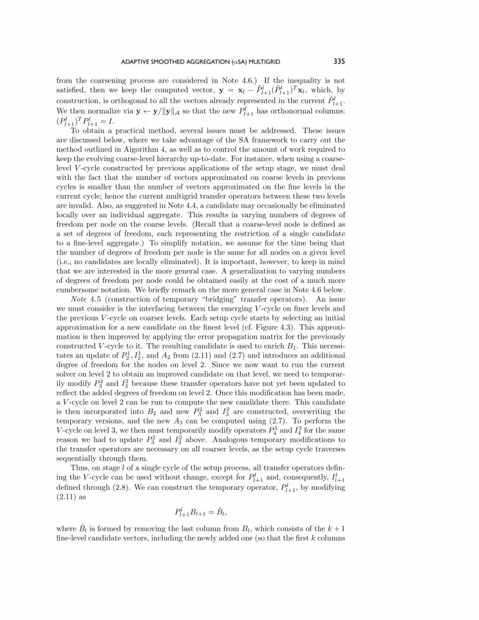
Note 4.5 (construction of temporary “bridging” transfer operators). An issuewe must consider is the interfacing between the emerging V -cycle on finer levels andthe previous V -cycle on coarser levels. Each setup cycle starts by selecting an initialapproximation for a new candidate on the finest level (cf. Figure 4.3). This approxi-mation is then improved by applying the error propagation matrix for the previouslyconstructed V -cycle to it. The resulting candidate is used to enrich B1. This necessi-tates an update of P 1

2 , I12 , and A2 from (2.11) and (2.7) and introduces an additional

degree of freedom for the nodes on level 2. Since we now want to run the currentsolver on level 2 to obtain an improved candidate on that level, we need to temporar-ily modify P 2

3 and I23 because these transfer operators have not yet been updated to

reflect the added degrees of freedom on level 2. Once this modification has been made,a V -cycle on level 2 can be run to compute the new candidate there. This candidateis then incorporated into B2 and new P 2

3 and I23 are constructed, overwriting the

temporary versions, and the new A3 can be computed using (2.7). To perform theV -cycle on level 3, we then must temporarily modify operators P 3

4 and I34 for the same

reason we had to update P 23 and I2

3 above. Analogous temporary modifications tothe transfer operators are necessary on all coarser levels, as the setup cycle traversessequentially through them.

Thus, on stage l of a single cycle of the setup process, all transfer operators defin-ing the V -cycle can be used without change, except for P ll+1 and, consequently, I

ll+1

defined through (2.8). We can construct the temporary operator, P ll+1, by modifying(2.11) as

P ll+1Bl+1 = Bl,

where Bl is formed by removing the last column from Bl, which consists of the k + 1fine-level candidate vectors, including the newly added one (so that the first k columns

336 BREZINA ET AL.

represent the same candidates as in the previous cycle). Since tentative prolongatorP ll+1 produced in this way is based only on fitting the first k vectors in Bl, the coarse-level matrix Al+1 resulting from the previous cycle of the αSA setup (described below)can be used on the next level. Thus, all the coarse operators for levels coarser than lcan be used without change. This has the advantage of reducing the amount of workto keep the V -cycle up-to-date on coarser, yet-to-be-traversed levels.

So far, we have considered only the case where all candidates are used locally.In the interest of keeping only the candidates that are essential to achieving goodconvergence properties, we now consider practical aspects of locally eliminating thecandidates where appropriate.

Note 4.6 (eliminating candidates locally as suggested in Note 4.4). When weeliminate a candidate locally over an aggregate as suggested in Note 4.4, the con-struction of the bridging operator above can be easily modified so that the multigridhierarchy constructed in the previous setup cycle can be used to apply a level l V -cycle in the current one. Since the procedure guarantees that the previously selectedcandidates are retained and only the newly computed candidate may be locally elim-inated, the V -cycle constructed in the previous setup cycle remains valid on coarserlevels as in the case of Note 4.5. The only difference now is that aggregates may havea variable number of associated candidates, and the construction of the temporarytransfer operator, P ll+1, described in Note 4.5 must account for this when removingthe column of Bl to construct Bl.

Note 4.7 (selection of the local quantities δA(x)). Our algorithm relies on localaggregate quantities δA(x) to decide whether to eliminate candidate x in aggregateA, and to guarantee that the computed candidates satisfy the global approximationproperty (4.1). This leads us to the choice

δA(x) =(card(A)Nl

)〈Alx,x〉ρ(Al)

,(4.7)

where card(A) denotes the number of nodes in aggregate A on level l, and Nl is thetotal number of nodes on that level. Note that

∑A δA(x) =

〈Alx,x〉ρ(Al)

for any x, so thiscan be used in local estimates (4.2) to guarantee (4.1).

Having discussed the modifications that may be necessary, we are now ready togive the algorithm for the general stage of αSA. Assume we are given a bound, K ∈ N,on the number of degrees of freedom per node on coarse levels, convergence factortolerance ε ∈ (0, 1), and aggregate quantities δA(x) such that

∑A δA(x) =

〈Alx,x〉ρ(Al)

.Then one step of the general setup stage proceeds as follows.

Algorithm 4 (one cycle of the general αSA setup stage).1. If the maximum number of degrees of freedom per node on level 2 equals K,

stop (the allowed number of coarse-level degrees of freedom has been reached).2. Create a copy of the current B1 for later use: B1 ← B1.3. Select a random x1 ∈ Rn1 and apply µ iterations of the current V -cycle,

denoting the kth iteration by xk1 :

xµ1 ← AMGµ1 (x

01,0), x1 ← xµ1 .

4. If 〈A1xµ1 ,x

µ1 〉 ≤ ε〈A1x

µ−11 ,xµ−1

1 〉, then stop (A1x = b1 can be solved quicklyenough by the current method).

5. Update B1 by extending its range with the new column x1:

B1 ← [B1,x1].


6. For l = 1, . . . , L− 2:(a) Define a new coarse-level matrix Bl+1 and transfer operator P ll+1 based

on (2.11), using Bl and decomposition AliNli=1. In creating P ll+1, somelocal components in Bl may be locally eliminated as suggested in Note 4.4.

(b) Construct the prolongator: I ll+1 = SlPll+1.

(c) Construct the coarse operator: Al+1 = (I ll+1)TAlI

ll+1.

(d) Reorder the columns of Bl+1 so that its last is xl+1, and let Bl+1 consistof all other columns of Bl+1.

(e) Create a “bridge” transfer operator P l+1l+2 to the coarser level with the old

Bl+1 by fitting all the vectors in Bl+1 except the last one; see Note 4.5.(f) Set the new “bridging” prolongator: I l+1

l+2 = Sl+1Pl+1l+2 .

(g) Make a copy: xl+1 ← xl+1.(h) Apply µ iterations: xl+1 ← AMGµ

l+1(xl+1,0).(i) If ( 〈Al+1xl+1,xl+1〉

〈Al+1xl+1,xl+1〉 )1/µ ≤ ε, then skip (d) through (j) in further passes

through step 6.(j) Update the coarse representation of candidate Bl+1:

Bl+1 ← [Bl+1,xl+1].

7. Update the latest fine-level candidate:

x1 ← I12I

23 . . . I

L−2L−1xL−1.(4.8)

8. Update B1 by extending the old copy with the newly computed x1:

B1 ← [B1,x1].

9. Create the V -cycle based on the current B1 using the standard SA setup de-scribed by Algorithm 2.

Algorithm 4, which is illustrated in Figure 4.3, starts from a V -cycle on inputand produces an improved V -cycle as output. It stops iterating when either theconvergence factor for the fine-level iteration in step 3 is acceptable (as measured instep 4) or the maximum number of iterations is reached. Note that, as with the initialstage, this general stage does not involve level L processing because the coarsest levelis assumed to be treated by a direct solver. Also as in the initial stage, once a levelis reached where the problem can be solved well by the current method, any furthercoarsening is constructed as in the standard SA.

Before presenting computational results, we consider several possible improve-ments intended to reduce the necessary number of cycles of the setup and the amountof work required to carry each cycle.

Note 4.8 (improving the quality of existing candidates). Many practical situ-ations, including fourth-order equations and systems of fluid and solid mechanics,require a set of multiple candidates to achieve optimal convergence. In the interestof keeping operator complexity as small as possible, it is imperative that the numberof candidates used to produce the final method be controlled. Therefore, ways ofimproving the quality of each candidate are of interest, to curb the demand for thegrowth in their number.

When the current V -cycle hierarchy is based on approximating at least two can-didates (in other words, the coarse problems feature at least two degrees of freedomper node), this can be easily accomplished as follows.

338 BREZINA ET AL.

Given B select x1

2

L

3 3 3

1

2 2 2P B = B x Last col. of B~

2 31

Run S. A. setup

New V-cycle

L–221x I I ... I xL–1

Set B [ B x ]1

L1

V–cycle on A x = 0 B [ B x ]1 1

11

2

3

Update x1~

2

1 1

1

2 22

1

22

L– 1

,

,P B = B x Last col. of B

1 1

2

V–cycle on A x = 0 B [ B x ]

Fig. 4.3 One step of general setup stage, Algorithm 4.

Assume that the currently available candidate vectors are x1, . . . ,xk. Considerone such candidate, say, xj, that we want to improve. We want to run a modifiedbut current V -cycle on the homogeneous problem, A1x = 0, using xj as the initialguess. The modification consists of disabling, in the coarse-grid correction process,the columns of the prolongator corresponding to the given candidate. That is, insteadof xl ← xl + I ll+1xl+1 in step 2(c) of Algorithm 1, we use

xl ← xl + I ll+1xl+1,

where xl+1 is obtained from xl+1 by setting to zero every entry corresponding tofine-level candidate xj. Thus, the columns of I ll+1 corresponding to xj are not usedin coarse-grid correction.

In this way, we come up with an improved candidate vector without restartingthe entire setup iteration from scratch and without adding a new candidate. Since wefocus on one component at a time and keep all other components intact, this modifiedV -cycle is expected to converge rapidly.

Note 4.9 (saving work). The reuse of current coarse-level components describedin Note 4.5 reduces the amount of work required to keep the V -cycle up-to-date. Ad-ditional work can be saved by performing the decomposition of nodes into disjointaggregates only during the setup of the initial V -cycle and then reusing this decom-position in later cycles. Yet further savings are possible in coarsening, assuming thecandidates are allowed to be locally eliminated according to Note 4.4. For instance,we can exploit the second-level matrix structure

A2 =[A2 XY Z

],

where A2 is the second-level matrix from the previous cycle. Thus, A2 need not berecomputed and can be obtained by a rank-one update of each block entry in A2.In a similar fashion, the new operators P ll+1, Bl+1 do not have to be recomputed in


each new setup cycle by the local QR decomposition noted in section 2. Instead, it ispossible to update each nodal entry in P ll+1, B

l+1 by a rank-one update on all coarselevels, where P ll+1, B

l+1 are the operators created by the previous setup cycle.

5. Numerical Experiments. To demonstrate the effectiveness of the proposedadaptive setup process, we present results obtained by applying the method to severalmodel problems. In these tests, the solver was stopped when the relative residualreached the value ε = 10−12 (unless otherwise specified). Ca = 10−3 was used for test(4.6) and parameter ε used in the adaptive setup was 0.1. The relaxation scheme forthe multigrid solver was symmetric Gauss–Seidel. While a Krylov subspace processis used often in practice, we present these results for a basic multigrid V -cycle withno acceleration scheme for clarity, unless explicitly specified otherwise.

All the experiments have been run on a notebook computer with a 1.6 GHz mo-bile Pentium 4 processor and 512 MB of RAM. For each experiment, we report thefollowing. The column denoted by “Iter” contains the number of iterations requiredto reduce the residual by the prescribed factor. The “Factor” column reports con-vergence factor measured as the geometric average of the residual reduction in thelast 10 iterations. In the “CPU” column, we report the total CPU times in secondsrequired to complete both the setup and iteration phases of the solver. In the col-umn “RelCPU,” we report the relative times to solution, with one unit defined as thetime required to solve the problem given the correct near-kernel components. In the“OpComp” column, we report the operator complexity associated with the V -cyclefor every run (we define operator complexity in the usual sense [19], as the ratio ofthe number of entries stored in all problem matrices on all levels divided by the num-ber of entries stored in the finest-level matrix). The “Candidates” column indicatesthe number of kernel vectors computed in the setup iteration (a value of “provided”means that complete kernel information was supplied to the solver, assuming standarddiscretization and ignoring scaling). Parameter µmax denotes the maximal number oftentative V -cycles allowed in computing each candidate.

In all the cases considered, the problem was modified either by scaling or byrotating each nodal entry in the system by a random angle (as described below).These modifications pose serious difficulties for classical algebraic iterative solversthat are not aware of such modifications.

For comparison, we also include the results for the unmodified problem, with asupplied set of kernel components. Not surprisingly, the standard algorithm (withoutbenefit of the adaptive process) performs poorly for the modified system when thedetails of this modification are kept from the solver, as we assume here.

Problem 1: Scaled 3D Poisson Problem. We start by considering a diagonallyscaled problem,

A← D−1/2AD−1/2,

where the original A is the matrix obtained by standard Q1 finite element discretiza-tion of the 3D Poisson operator on a cube and D is a diagonal matrix with entries10β , where β ∈ [−σ,+σ] is chosen randomly. Table 5.1 shows the results for differentvalues of parameter σ and different levels of refinement. Using the supplied kernelyields good convergence factors for the unmodified problem, but the performance ispoor and deteriorates with increased problem size when used with σ = 0. In contrast,the adaptive process, starting from a random approximation, recovers the convergenceproperties associated with the standard Poisson problem (σ = 0), even for the scaledcase, with convergence that appears bounded independent of the problem size.

340 BREZINA ET AL.

Table 5.1 Misscaled 3D Poisson problems with 68,921 and 1,030,301 degrees of freedom; using ε =10−8.

σ Candidates µmax Iter Factor CPU RelCPU OpComp

Poisson problem with 68,921 degrees of freedom0 provided N/A 9 0.100 3.65 1.00 1.0380 1 5 9 0.100 4.09 1.12 1.0386 provided N/A 150 0.871 43.76 11.99 1.0386 1 5 10 0.126 4.27 1.17 1.038

Poisson problem with 1,030,301 degrees of freedom0 provided N/A 9 0.093 58.43 1.00 1.0390 1 5 9 0.099 80.05 1.37 1.0396 provided N/A 690 0.970 3,252.80 55.67 1.0396 1 5 9 0.096 88.23 1.51 1.039

Table 5.2 Scaled 2D elasticity problems with 80,400 and 181,202 degrees of freedom. Iteration countsmarked with an asterisk indicate that residual reduction by 1012 was not achieved beforethe maximum number of iterations was reached.


2D elasticity problem, 80,400 degrees of freedom0 3 provided N/A 17 0.21 9.16 1.00 1.270 3 6 23 0.37 21.16 2.31 1.270 3 15 18 0.23 26.65 2.91 1.276 3 provided N/A 299 0.92 133.55 14.58 1.276 3 6 25 0.38 22.26 2.43 1.276 3 15 18 0.25 27.30 2.98 1.27

2D elasticity problem, 181,202 degrees of freedom0 3 provided N/A 23 0.35 22.85 1.00 1.280 3 15 267 0.937 272.14 11.91 1.270 4 15 26 0.422 75.18 3.29 1.500 4 20 26 0.439 86.60 3.79 1.500 5 15 20 0.314 88.20 3.86 1.786 3 provided N/A 5, 000∗ 0.996 4,559.95 199.56 1.286 4 15 23 0.367 74.95 3.28 1.506 4 20 19 0.302 76.78 3.36 1.506 5 10 14 0.173 69.46 3.04 1.78

Problem 2: Scaled 2D Elasticity. Here we consider a diagonally scaled matrixarising in 2D elasticity. Diagonal entries of D are again defined as 10β , with β ∈[−σ,+σ] chosen randomly. The original matrix is the discrete operator for the plane-strain elasticity formulation over a square domain using bilinear finite elements ona uniform mesh, with a Poisson ratio of ν = 0.3 and Dirichlet boundary conditionsspecified only along the “West” side of the domain. The results in Table 5.2 followa pattern similar to those for the Poisson problem. Note, however, that more thanthe usual three candidate vectors are now needed to achieve convergence propertiessimilar to those observed with the unmodified problem for which the correct set ofthree rigid body modes is provided by the user. For the scaled problem, however,


Table 5.3 Rotated 2D elasticity problems with 80,400 and 181,202 degrees of freedom. Iterationcounts marked with an asterisk indicate that residual reduction by 1012 was not achievedbefore the limit on the number of iterations was reached.

Rotated Candidates µmax Iter Factor CPU RelCPU OpComp

2D elasticity problem with 80,400 degrees of freedomNO 3 provided N/A 17 0.21 9.16 s 1.00 1.27NO 3 15 18 0.23 26.66 2.91 1.27YES 3 provided N/A 1,329 0.99 587.80 64.17 1.27YES 3 15 19 0.27 27.8464 3.04 1.27

2D elasticity problem with 181,202 degrees of freedomNO 3 provided N/A 23 0.35 22.85 s 1.00 1.28NO 3 15 18 0.23 66.49 2.91 1.28YES 3 provided N/A 5, 000∗ 0.999 3,968.36 173.67 1.28YES 3 20 135 0.885 170.23 7.45 1.28YES 4 15 27 0.488 77.46 3.39 1.50YES 4 20 21 0.395 79.29 3.47 1.50YES 5 6 18 0.34 60.78 2.66 1.78YES 5 10 15 0.233 72.66 3.18 1.78

supplying the rigid body modes computed based on the problem geometry leads, asexpected, to dismal performance of the standard solver.

Problem 3: Locally Rotated 2D Elasticity. This set of experiments is basedagain on the 2D elasticity problem, but now each nodal block is rotated by a randomangle β ∈ [0, π],

A← QTAQ,

where Q is a nodal block-diagonal matrix consisting of rotations with random angles.The results in Table 5.3 show that αSA can recover good convergence factors for boththe unmodified and the modified systems. Without the adaptive procedure, our basicalgebraic solver could not solve the modified matrix problem in a reasonable amountof time.

Problem 4: Locally Rotated 3D Elasticity. This set of experiments demonstratesperformance of the method when a higher number of candidates is required. We con-sider a 3D elasticity problem with local rotations. This is done to maintain locallyorthogonal coordinates but is otherwise a random rotation of the three degrees of free-dom at each node. The model problem we start from is linearized elasticity discretizedusing trilinear finite elements over a uniform mesh. Dirichlet boundary conditions arespecified on the “West” face of the cube, and the Poisson ratio is set to ν = 0.3. Theresults in Table 5.4 show that, even for the modified system, the adaptive methodcan again recover good convergence factors. Furthermore, our current method mim-ics the convergence of SA for the unmodified problem with the supplied set of rigidbody modes. In this set of experiments, we can get close to the ideal iteration countsusing just six candidates. We see that using one extra candidate can improve conver-gence properties and in some cases actually lower the overall cost of the total timeto solution. This is done at the price of a small increase in operator complexity. Forproblems with multiple right sides, the more expensive setup would be performed onlyonce, and using the extra candidate may then be preferred.

342 BREZINA ET AL.

Table 5.4 Rotated 3D elasticity problems with 114,444 and 201,720 degrees of freedom.

Rotated Candidates µmax Iter Factor CPU RelCPU OpComp

3D elasticity problem with 114,444 degrees of freedomNO 6 provided N/A 16 0.20 29.97 1.00 1.159NO 6 15 20 0.27 189.11 6.31 1.159NO 7 15 17 0.21 215.78 7.20 1.217YES 6 provided N/A 587 0.97 913.49 30.48 1.159YES 6 15 16 0.22 184.32 6.15 1.159YES 7 10 15 0.20 171.73 5.73 1.217YES 7 15 15 0.20 210.99 7.04 1.217

3D elasticity problem with 201,720 degrees of freedomNO 6 provided N/A 16 0.20 50.33 1.00 1.153NO 6 15 21 0.31 319.60 6.35 1.153NO 7 10 17 0.216 297.95 5.92 1.209NO 7 15 17 0.209 363.38 7.22 1.209YES 6 provided N/A 739 0.97 1,924.62 38.24 1.153YES 6 15 16 0.23 308.02 6.12 1.153YES 7 10 15 0.20 301.98 6.00 1.209YES 7 15 14 0.16 357.85 7.11 1.209

Figures 5.1 and 5.2 illustrate the difference between candidates computed for thelocally rotated problem and the original (unrotated) problem, respectively. While thecandidate representing the algebraically smooth error corresponding to the originalproblem exhibits also smoothness in the geometric sense, for the rotated problemsuch smoothness is observed only at the Dirichlet boundary, where the solution iszero regardless of the rotation. For the sake of visualization, the candidates depictedin Figures 5.1 and 5.2 have been computed by running a smaller problem with 86,490degrees of freedom.

Problem 5: 3D Elasticity with Discontinuous Coefficients. The final exampledemonstrates performance of the adaptive method for an elasticity problem featuringdiscontinuities in the Young modulus. Here we consider a 3D elasticity problem inwhich the Poisson ratio is fixed at 0.32, while the Young modulus is allowed to varyrandomly between the elements. We consider two cases: a case of coefficients varyingrandomly with uniform distribution in the interval (1, 10σ) and the case where thedistribution is exponential; i.e., the Young modulus is computed as 10(σr), where ris generated randomly with uniform distribution in (0, 1). Keeping with the usualpractice of employing Krylov method acceleration for problems with coefficient dis-continuities, in this experiment we use our adaptive method as a preconditioner inthe conjugate gradient method. The iteration was stopped once the initial residualwas reduced by a factor of 108. Table 5.5 compares the results obtained by usingour adaptive scheme, starting from a random initial guess, to the results obtainedwhen the method based on a priori knowledge of the appropriate rigid body modes isemployed as a preconditioner. The table indicates that, using the adaptive procedurewithout a priori knowledge of the problem geometry, we can essentially recover therates of the method based on the knowledge of the rigid body modes.

The topic of problems with discontinuous coefficients and the appropriate modi-fications to the basic SA method will be studied in a future paper.


Fig. 5.1 Candidate representing algebraically smooth error for the 3D elasticity problem modifiedby applying random local rotations.

Fig. 5.2 Candidate computed for the 3D elasticity problem without the modification by local rotationsexhibits geometric smoothness.

344 BREZINA ET AL.

Table 5.5 3D elasticity problem, 201,720 degrees of freedom, with Young modulus featuring randomjumps in (1, 10σ).


Elasticity problem with uniformly distributed coefficient jumps

2 6 provided N/A 8 0.0734 24.22 1.00 1.152 6 10 13 0.2209 219.34 9.05 1.152 7 10 11 0.1866 266.29 10.99 1.21

3 6 provided N/A 8 0.0765 24.23 1.00 1.153 6 10 13 0.2154 218.57 9.02 1.153 7 10 11 0.1861 265.70 10.96 1.21

4 6 provided N/A 8 0.0768 24.56 1.00 1.154 6 10 12 0.2081 219.26 8.93 1.154 7 10 11 0.1648 264.38 10.76 1.21

Elasticity problem with exponentially distributed coefficient jumps

2 6 provided N/A 9 0.1146 25.99 1.00 1.152 6 10 16 0.3048 225.52 8.68 1.152 7 10 12 0.2141 267.72 10.30 1.21

3 6 provided N/A 14 0.2466 35.68 1.00 1.153 6 10 22 0.4179 237.56 6.76 1.153 7 10 16 0.3095 275.62 7.84 1.21

4 6 provided N/A 20 0.3948 49.99 1.00 1.154 6 10 30 0.5316 255.43 5.11 1.154 7 10 21 0.4040 289.39 5.79 1.21

5 6 provided N/A 32 0.5545 73.63 1.00 1.155 6 10 46 0.6695 292.35 3.97 1.155 6 20 36 0.5980 402.75 5.47 1.215 7 10 37 0.6020 324.19 4.40 1.215 7 15 27 0.4966 381.16 5.17 1.21

Note 5.1. The operator complexities in all of the test problems remain below2. Moreover, these complexities improve somewhat in three dimensions, compared totwo dimensions, due largely to the increased speed of aggregation coarsening. It isalso worth mentioning that the increasing size of the coarse matrix block entries dueto the increasing number of candidates does not significantly impact the time neededto perform one iteration of the solver, apparently due to the more efficient memoryaccess afforded by blocking.

6. Conclusions. This paper develops a new multilevel method to tackle problemsthat, to date, have been very difficult to handle by AMG methods. At the expenseof a somewhat more costly setup stage and more intricate implementation, we designa method that has, thus far, proved successful at solving such problems. We observethat the convergence properties of the method seem very insensitive to modifications ofthe algebraic system by scaling or nodal rotation. Moreover, the solver is flexible andcan benefit from extra information supplied about the problem. If such informationis lacking or incorrect, then αSA can act as a full black-box solver. Despite thegrowing number of degrees of freedom per coarse-level node as the method evolves,the overall cost of one step of the final iteration grows only modestly because of betterutilization of cache memory due to dense matrix operations on the nodal blocks.


Operator complexity remains at reasonable levels and actually seems to improve withincreasing spatial dimension.

The construction of the tentative prolongator in the setup phase involves restric-tion of the candidate functions to an aggregate and subsequent local orthogonalizationof these functions. It is therefore suitable for parallel processing as long as the ag-gregates are local to the processor. Parallelization of the underlying SA solver isin the testing stage. When it is completed, then αSA should also benefit from theparallel speedup. The parallel version is also expected to gain better parallel scalabil-ity by replacing the traditionally used Gauss–Seidel relaxation with the polynomialsmoothing procedures investigated recently in [1]. The performance of the parallelimplementation will depend on the quality of the parallel matrix-vector product.

Future development will concentrate on extending features of the underlyingmethod on which αSA relies and on developing theory beyond the heuristics pre-sented here. Although most decisions are currently made by the code at runtime,much remains to be done to fully automate the procedure, such as determining cer-tain tolerances that are now input by the user. We plan to explore the possibility ofsetting or updating these parameters at runtime based on the characteristics of theproblem at hand. A related work in progress [7] explores adaptive ideas suitable inthe context of the standard AMG method.

REFERENCES

[1] M. Adams, M. Brezina, J. Hu, and R. Tuminaro, Parallel multigrid smoothing: Polynomialversus Gauss-Seidel, J. Comput. Phys., 188 (2003), pp. 593–610.

[2] J. Bramble, J. Pasciak, J. Wang, and J. Xu, Convergence estimates for multigrid algorithmwithout regularity assumptions, Math. Comp., 57 (1991), pp. 23–45.

[3] A. Brandt, Lecture given at CASC, Lawrence Livermore National Lab, Livermore, CA, 2001.[4] A. Brandt, S. F. McCormick, and J. W. Ruge, Algebraic multigrid (AMG) for sparse matrix

equations, in Sparsity and Its Applications, D. J. Evans, ed., Cambridge University Press,Cambridge, UK, 1984, pp. 257–284.

[5] A. Brandt and D. Ron, Multigrid solvers and multilevel optimization strategies, in MultilevelOptimization in VLSICAD, Comb. Optim. 14, J. Cong and J. R. Shinnerl, eds., KluwerAcademic, Dordrecht, The Netherlands, 2003, pp. 1–69.

[6] M. Brezina, A. J. Cleary, R. D. Falgout, V. E. Henson, J. E. Jones, T. A. Manteuffel,

S. F. McCormick, and J. W. Ruge, Algebraic multigrid based on element interpolation(AMGe), SIAM J. Sci. Comput., 22 (2000), pp. 1570–1592.

[7] M. Brezina, R. Falgout, S. MacLachlan, T. Manteuffel, S. F. McCormick, and J. W.

Ruge, Adaptive Algebraic Multigrid (αAMG), SIAM J. Sci. Comput., submitted.[8] M. Brezina, C. I. Heberton, J. Mandel, and P. Vanek, An Iterative Method with Conver-

gence Rate Chosen A Priori, UCD/CCM report 140, Center for Computational Mathemat-ics, University of Colorado at Denver, Denver, CO, 1999; available online from http://www-math.cudenver.edu/ccmreports/rep140.ps.gz.

[9] M. Brezina and P. Vanek, A black-box iterative solver based on a two-level Schwarz method,Computing, 63 (1999), pp. 233–263.

[10] W. Briggs, V. E. Henson, and S. F. McCormick, A Multigrid Tutorial, 2nd ed., SIAM,Philadelphia, 2000.

[11] T. Chartier, Element-Based Algebraic Multigrid (AMGe) and Spectral AMGe, Ph.D. thesis,University of Colorado at Boulder, Boulder, CO, 2001.

[12] T. Chartier, R. D. Falgout, V. E. Henson, J. Jones, T. Manteuffel, S. McCormick,

J. Ruge, and P. S. Vassilevski, Spectral AMGe (ρAMGe), SIAM J. Sci. Comput., 25(2003), pp. 1–26.

[13] J. Fish and V. Belsky, Generalized aggregation multilevel solver, Internat. J. Numer. MethodsEngrg., 40 (1997), pp. 4341–4361.

[14] S. F. McCormick and J. W. Ruge, Algebraic multigrid methods applied to problems in com-putational structural mechanics, in State of the Art Surveys on Computational Mechanics,A. K. Noor and J. T. Oden, eds., ASME, New York, 1989, pp. 237–270.

346 BREZINA ET AL.

[15] J. W. Ruge, Algebraic multigrid (AMG) for geodetic survey problems, in Proceedings of theInternational Multigrid Conference, Copper Mountain, CO, 1983.

[16] J. W. Ruge, Final Report on AMG02, report, Gesellschaft fuer Mathematik und Datenverar-beitung, St. Augustin, 1985, GMD, contract 5110/022090.

[17] J. W. Ruge, AMG for problems of elasticity, Appl. Math. Comput., 19 (1986), pp. 293–309.[18] J. W. Ruge and K. Stuben, Efficient solution of finite difference and finite element equations

by algebraic multigrid (AMG), in Multigrid Methods for Integral and Differential Equa-tions, The Institute of Mathematics and Its Applications Conference Series, D. J. Paddonand H. Holstein, eds., Clarendon Press, Oxford, UK, 1985, pp. 169–212.

[19] J. W. Ruge and K. Stuben, Algebraic multigrid (AMG), in Multigrid Methods, FrontiersAppl. Math. 3, S. F. McCormick, ed., SIAM, Philadelphia, 1987, pp. 73–130.

[20] P. Vanek, M. Brezina, and J. Mandel, Convergence of algebraic multigrid based on smoothedaggregation, Numer. Math., 88 (2001), pp. 559–579.

[21] P. Vanek, Acceleration of convergence of a two-level algorithm by smoothing transfer operator,Appl. Math., 37 (1992), pp. 265–274.

[22] P. Vanek, M. Brezina, and R. Tezaur, Two-grid method for linear elasticity on unstructuredmeshes, SIAM J. Sci. Comput., 21 (1999), pp. 900–923.

[23] P. Vanek, J. Mandel, and M. Brezina, Algebraic multigrid by smoothed aggregation forsecond and fourth order elliptic problems, Computing, 56 (1996), pp. 179–196.

[24] R. Varga, Matrix Iterative Analysis, Prentice-Hall, Englewood Cliffs, NJ, 1962.

adaptive smoothed aggregation ($\\alpha$sa) multigrid

Documents