phantom: a smoothed particle hydrodynamics and

Publications of the Astronomical Society of Australia (PASA), Vol. 35, e031, 82 pages (2018).© Astronomical Society of Australia 2018; published by Cambridge University Press.doi:10.1017/pasa.2018.25

PHANTOM: A Smoothed Particle Hydrodynamics andMagnetohydrodynamics Code for Astrophysics

Daniel J. Price1,18, James Wurster2,1, Terrence S. Tricco3,1, Chris Nixon4, Stéven Toupin5, Alex Pettitt6,Conrad Chan1, Daniel Mentiplay1, Guillaume Laibe7, Simon Glover8, Clare Dobbs2, Rebecca Nealon4,1,David Liptai1, Hauke Worpel9,1, Clément Bonnerot10, Giovanni Dipierro4, Giulia Ballabio4,Enrico Ragusa11, Christoph Federrath12, Roberto Iaconi13, Thomas Reichardt13, Duncan Forgan14,Mark Hutchison15,16,1, Thomas Constantino2, Ben Ayliffe17,1, Kieran Hirsh1 and Giuseppe Lodato11

1Monash Centre for Astrophysics (MoCA) and School of Physics and Astronomy, Monash University, Vic. 3800, Australia2School of Physics, University of Exeter, Exeter EX4 4QL, UK3Canadian Institute for Theoretical Astrophysics (CITA), University of Toronto, Toronto, ON M5S 3H8, Canada4Theoretical Astrophysics Group, Department of Physics & Astronomy, University of Leicester, Leicester LE1 7RH, UK5Institut d’Astronomie et d’Astrophysique (IAA), Université Libre de Bruxelles (ULB), CP226, Boulevard du Triomphe B1050 Brussels, Belgium6Department of Cosmosciences, Hokkaido University, Sapporo 060-0810, Japan7Centre de Recherche Astrophysique de Lyon, Univ Lyon, ENS de Lyon, CNRS, Saint-Genis-Laval F-69230, France8Institut für Theoretische Astrophysik, Zentrum für Astronomie der Universität Heidelberg, D-69120 Heidelberg, Germany9AIP Potsdam, An der Sternwarte 16, 14482 Potsdam, Germany10Leiden Observatory, Leiden University, PO Box 9513, NL-2300 RA Leiden, the Netherlands11Dipartimento di Fisica, Università Degli Studi di Milano, Via Celoria 16, Milano 20133, Italy12Research School of Astronomy and Astrophysics, Australian National University, Canberra ACT 2611, Australia13Department of Physics and Astronomy, Macquarie University, 2109 Sydney, Australia14St Andrews Centre for Exoplanet Science and School of Physics and Astronomy, University of St. Andrews, North Haugh, St. Andrews,Fife KY16 9SS, UK15Physikalisches Institut, Universität Bern, Gesellschaftstrasse 6, 3012 Bern, Switzerland16Institute for Computational Science, University of Zurich, Winterthurerstrasse 190, CH-8057 Zürich, Switzerland17Met Office, FitzRoy Road, Exeter EX1 3PB, UK18Email: [email protected]

(RECEIVED February 14, 2017; ACCEPTED June 15, 2018)

Abstract

We present PHANTOM, a fast, parallel, modular, and low-memory smoothed particle hydrodynamics and magnetohy-drodynamics code developed over the last decade for astrophysical applications in three dimensions. The code has beendeveloped with a focus on stellar, galactic, planetary, and high energy astrophysics, and has already been used widelyfor studies of accretion discs and turbulence, from the birth of planets to how black holes accrete. Here we describeand test the core algorithms as well as modules for magnetohydrodynamics, self-gravity, sink particles, dust–gas mix-tures, H2 chemistry, physical viscosity, external forces including numerous galactic potentials, Lense–Thirring precession,Poynting–Robertson drag, and stochastic turbulent driving. PHANTOM is hereby made publicly available.

Keywords: accretion, accretion disks – hydrodynamics – ISM: general – magnetohydrodynamics (MHD) – methods:numerical

1 INTRODUCTION

Numerical simulations are the ‘third pillar’ of astrophysics,standing alongside observations and analytic theory. Since itis difficult to perform laboratory experiments in the relevantphysical regimes and over the correct range of length andtimescales involved in most astrophysical problems, we turninstead to ‘numerical experiments’ in the computer for un-derstanding and insight. As algorithms and simulation codesbecome ever more sophisticated, the public availability of

simulation codes has become crucial to ensure that these ex-periments can be both verified and reproduced.

PHANTOM is a smoothed particle hydrodynamics (SPH)code developed over the last decade. It has been used widelyfor studies of turbulence (e.g. Kitsionas et al. 2009; Price& Federrath 2010; Price, Federrath, & Brunt 2011), accre-tion (e.g. Lodato & Price 2010; Nixon, King, & Price 2012a;Rosotti, Lodato, & Price 2012), star formation includingnon-ideal magnetohydrodynamics (MHD) (e.g. Wurster et al.2016, Wurster, Price, & Bate 2017), star cluster formation

1

https://doi.org/10.1017/pasa.2018.25Downloaded from https://www.cambridge.org/core. IP address: 65.21.229.84, on 04 Feb 2022 at 11:36:48, subject to the Cambridge Core terms of use, available at https://www.cambridge.org/core/terms.

https://doi.org/10.1017/pasa.2018.25

http://orcid.org/0000-0002-4716-4235

http://orcid.org/0000-0003-0688-5332

http://orcid.org/0000-0002-6238-9096

https://orcid.org/0000-0002-2137-4146

https://orcid.org/0000-0002-3662-3942

https://orcid.org/0000-0002-7316-9240

http://orcid.org/0000-0002-5526-8798

https://orcid.org/0000-0001-6708-1317

https://orcid.org/0000-0002-4578-297X

https://orcid.org/0000-0003-0856-679X

http://orcid.org/0000-0002-4856-1750

https://orcid.org/0000-0002-5042-9070

http://orcid.org/0000-0002-7185-5458

https://orcid.org/0000-0001-5378-7749

https://orcid.org/0000-0002-0706-2306

https://orcid.org/0000-0003-4899-4465

https://orcid.org/0000-0003-1175-4388

https://orcid.org/0000-0003-4543-8711

https://orcid.org/0000-0002-0758-4446

https://orcid.org/0000-0001-5647-5097

https://orcid.org/0000-0002-2357-7692

mailto:[email protected]


https://www.cambridge.org/core

https://www.cambridge.org/core/terms

2 Price et al.

(Liptai et al. 2017), and for studies of the Galaxy (Pettitt et al.2014; Dobbs et al. 2016), as well as for simulating dust–gasmixtures (e.g. Dipierro et al. 2015; Ragusa et al. 2017; Tricco,Price, & Laibe 2017). Although the initial applications andsome details of the basic algorithm were described in Price &Federrath (2010), Lodato & Price (2010), and Price (2012a),the code itself has never been described in detail and, untilnow, has remained closed source.

One of the initial design goals of PHANTOM was to have alow memory footprint. A secondary motivation was the needfor a public SPH code that is not primarily focused on cos-mology, as in the highly successful GADGET code (Springel,Yoshida, & White 2001; Springel 2005). The needs of dif-ferent communities produce rather different outcomes in thecode. For cosmology, the main focus is on simulating thegravitational collapse of dark matter in large volumes of theuniverse, with gas having only a secondary effect. This is re-flected in the ability of the public GADGET-2 code to scaleto exceedingly large numbers of dark matter particles, yetneglecting elements of the core SPH algorithm that are es-sential for stellar and planetary problems, such as the Morris& Monaghan (1997) artificial viscosity switch [c.f. the de-bate between Bauer & Springel (2012) and Price (2012b)], theability to use a spatially variable gravitational force softening(Bate & Burkert 1997; Price & Monaghan 2007) or any kindof artificial conductivity, necessary for the correct treatmentof contact discontinuities (Chow & Monaghan 1997; Price& Monaghan 2005; Rosswog & Price 2007; Price 2008).Almost all of these have since been implemented in develop-ment versions of GADGET-3 (e.g. Iannuzzi & Dolag 2011;Beck et al. 2016; see recent comparison project by Semboliniet al. 2016) but remain unavailable or unused in the pub-lic version. Likewise, the implementation of dust, non-idealMHD, and other physics relevant to star and planet formationis unlikely to be high priority in a code designed for studyingcosmology or galaxy formation.

Similarly, the SPHNG code (Benz et al. 1990; Bate 1995)has been a workhorse for our group for simulations of starformation (e.g. Price & Bate 2007, 2009; Price, Tricco, &Bate 2012; Lewis, Bate, & Price 2015) and accretion discs(e.g. Lodato & Rice 2004; Cossins, Lodato, & Clarke 2009),contains a rich array of physics necessary for star and planetformation including all of the above algorithms, but the legacynature of the code makes it difficult to modify or debug andthere are no plans to make it public.

GASOLINE (Wadsley, Stadel, & Quinn 2004) is anothercode that has been widely and successfully used for galaxyformation simulations, with its successor, GASOLINE 2(Wadsley et al. 2017), recently publicly released. Hubberet al. (2011) have developed SEREN with similar goals toPHANTOM, focused on star cluster simulations. SEREN thuspresents more advanced N-body algorithms compared towhat is in PHANTOM but does not yet include magnetic fields,dust, or H2 chemistry.

A third motivation was the need to distinguish betweenthe ‘high performance’ code used for 3D simulations from

simpler codes used to develop and test algorithms, such as ouralready-public NDSPMHD code (Price 2012a). PHANTOM isdesigned to ‘take what works and make it fast’, rather thancontaining options for every possible variation on the SPHalgorithm. Obsolete options are actively deleted.

The initial release of PHANTOM has been developed with afocus on stellar, planetary, and Galactic astrophysics, as wellas accretion discs. In this first paper, coinciding with the firststable public release, we describe and validate the core algo-rithms as well as some example applications. Various novelaspects and optimisation strategies are also presented. Thispaper is an attempt to document in detail what is currentlyavailable in the code, which include modules for MHD, dust–gas mixtures, self-gravity, and a range of other physics. Thepaper is also designed to serve as guide to the correct useof the various algorithms. Stable releases of PHANTOM areposted on the web1, while the development version and wikidocumentation are available on the BITBUCKET platform2.

The paper is organised as follows: We describe the nu-merical methods in Section 2 with corresponding numer-ical tests in Section 5. We cover SPH basics (Section2.1), our implementation of hydrodynamics (Sections 2.2and 5.1), the timestepping algorithm (Section 2.3), exter-nal forces (Sections 2.4 and 5.2), turbulent forcing (Sections2.5 and 6.1), accretion disc viscosity (Sections 2.6 and 5.3),Navier–Stokes viscosity (Sections 2.7 and 5.4), sink parti-cles (Sections 2.8 and 5.5), stellar physics (Section 2.9),MHD (Sections 2.10 and 5.6), non-ideal MHD (Sections 2.11and 5.7), self-gravity (Sections 2.12 and 5.8), dust–gas mix-tures (Sections 2.13 and 5.9), ISM chemistry and cooling(Sections 2.14 and 5.10), and particle injection (Section 2.15).We present the algorithms for generating initial conditions inSection 3. Our approach to software engineering is describedin Section 4. We give five examples of recent applicationshighlighting different aspects of PHANTOM in Section 6. Wesummarise in Section 7.

2 NUMERICAL METHOD

PHANTOM is based on the SPH technique, invented by Lucy(1977) and Gingold & Monaghan (1977) and the subject ofnumerous reviews (Benz 1990; Monaghan 1992, 2005, 2012;Rosswog 2009; Springel 2010; Price 2012a).

In the following, we adopt the convention that a, b, and crefer to particle indices; i, j, and k refer to vector or tensorindices; and n and m refer to indexing of nodes in the treecode.

2.1. Fundamentals

2.1.1. Lagrangian hydrodynamics

SPH solves the equations of hydrodynamics in Lagrangianform. The fluid is discretised onto a set of ‘particles’ of massm that are moved with the local fluid velocity v. Hence, the

1 https://phantomsph.bitbucket.io/2 https://bitbucket.org/danielprice/phantom

PASA, 35, e031 (2018)doi:10.1017/pasa.2018.25


https://phantomsph.bitbucket.io/

https://bitbucket.org/danielprice/phantom





Phantom 3

two basic equations common to all physics in PHANTOM are

drdt

= v, (1)

dρ

dt= −ρ(∇ · v), (2)

where r is the particle position and ρ is the density. Theseequations use the Lagrangian time derivative, d/dt ≡ ∂/∂t +v · ∇, and are the Lagrangian update of the particle positionand the continuity equation (expressing the conservation ofmass), respectively.

2.1.2. Conservation of mass in SPH

The density is computed in PHANTOM using the usual SPHdensity sum

ρa =∑

b

mbW (|ra − rb|, ha ), (3)

where a and b are particle labels, m is the mass of the par-ticle, W is the smoothing kernel, h is the smoothing length,and the sum is over neighbouring particles (i.e. those withinRkernh, where Rkern is the dimensionless cut-off radius of thesmoothing kernel). Taking the Lagrangian time derivative of(3), one obtains the discrete form of (2) in SPH

dρa

dt= 1

�a

∑b

mb(va − vb) · ∇aWab(ha), (4)

where Wab(ha) ≡ W (|ra − rb|, ha) and �a is a term related tothe gradient of the smoothing length (Springel & Hernquist2002; Monaghan 2002) given by

�a ≡ 1 − ∂ha

∂ρa

∑b

mb∂Wab(ha)

∂ha. (5)

Equation (4) is not used directly to compute the density inPHANTOM, since evaluating (3) provides a time-independentsolution to (2) (see e.g. Monaghan 1992; Price 2012a for de-tails). The time-dependent version (4) is equivalent to (3)up to a boundary term (see Price 2008) but is only used inPHANTOM to predict the smoothing length at the nexttimestep in order to reduce the number of iterations requiredto evaluate the density (see below).

Since (3)–(5) all depend on the kernel evaluated on neigh-bours within Rkern times ha, all three of these summationsmay be computed simultaneously using a single loop overthe same set of neighbours. Details of the neighbour findingprocedure are given in Section 2.1.7.

2.1.3. Setting the smoothing length

The smoothing length itself is specified as a function of theparticle number density, n, via

ha = hfactn−1/3a = hfact

(ma

ρa

)1/3

, (6)

where hfact is the proportionality factor specifying thesmoothing length in terms of the mean local particle spac-ing and the second equality holds only for equal mass par-

Table 1. Compact support radii, variance, standard deviation, rec-ommended ranges of hfact, and recommended default hfact settings(hd

fact) for the kernel functions available in PHANTOM.

Kernel Rkern σ 2/h2 σ /h hfact hdfact Nneigh

M4 2.0 9/10 0.95 1.0–1.2 1.2 57.9M5 2.5 23/20 1.07 1.0–1.2 1.2 113M6 3.0 7/5 1.18 1.0–1.1 1.0 113C2 2.0 4/5 0.89 �1.35 1.4 92C4 2.0 8/13 0.78 �1.55 1.6 137C6 2.0 1/2 0.71 �1.7 2.2 356

ticles, which are enforced in PHANTOM. The restriction toequal mass particles means that the resolution strictly fol-lows mass, which may be restrictive for problems involvinglarge density contrasts (e.g. Hutchison et al. 2016). However,our view is that the potential pitfalls of unequal mass particles(see e.g. Monaghan & Price 2006) are currently too great toallow for a robust implementation in a public code.

As described in Price (2012a), the proportionality constanthfact can be related to the mean neighbour number accordingto

Nneigh = 4

3π (Rkernhfact )

3, (7)

however, this is only equal to the actual neighbour numberfor particles in a uniform density distribution (more specif-ically, for a density distribution with no second derivative),meaning that the actual neighbour number varies. The de-fault setting for hfact is 1.2, corresponding to an average of57.9 neighbours for a kernel truncated at 2h (i.e. for Rkern = 2)in three dimensions. Table 1 lists the settings recommendedfor different choices of kernel. The derivative required in (5)is given by

∂ha

∂ρa= −3ha

ρa. (8)

2.1.4. Iterations for h and ρ

The mutual dependence of ρ and h means that a rootfind-ing procedure is necessary to solve both (3) and (6) simulta-neously. The procedure implemented in PHANTOM followsPrice & Monaghan (2004b, 2007), solving, for each particle,the equation

f (ha ) = ρsum(ha ) − ρ(ha) = 0, (9)

where ρsum is the density computed from (3) and

ρ(ha) = ma(hfact/ha)3, (10)

from (6). Equation (9) is solved with Newton–Raphson iter-ations:

ha,new = ha − f (ha )

f ′(ha), (11)

PASA, 35, e031 (2018)doi:10.1017/pasa.2018.25






4 Price et al.

where the derivative is given by

f ′(ha) =∑

b

mb∂Wab(ha)

∂ha− ∂ρa

∂ha= −3ρa

ha�a. (12)

The iterations proceed until |ha, new − ha|/ha, 0 < εh, whereha, 0 is the smoothing length of particle a at the start of theiteration procedure and εh is the tolerance. The convergencewith Newton–Raphson is fast, with a quadratic reduction inthe error at each iteration, meaning that no more than 2–3iterations are required even with a rapidly changing densityfield. We avoid further iterations by predicting the smoothinglength from the previous timestep according to

h0a = ha + �t

dha

dt= ha + �t

∂ha

∂ρa

dρa

dt, (13)

where dρa/dt is evaluated from (4).Since h and ρ are mutually dependent, we store only the

smoothing length, from which the density can be obtained atany time via a function call evaluating ρ(h). The default valueof εh is 10−4 so that h and ρ can be used interchangeably. Set-ting a small tolerance does not significantly change the com-putational cost, as the iterations quickly fall below a toleranceof ‘one neighbour’ according to (7), so any iterations beyondthis refer to loops over the same set of neighbours which canbe efficiently cached. However, it is important that the toler-ance may be enforced to arbitrary precision rather than beingan integer as implemented in the public version of GADGET,since (9) expresses a mathematical relationship between hand ρ that is assumed throughout the derivation of the SPHalgorithm (see discussion in Price 2012a). The precision towhich this is enforced places a lower limit on the total energyconservation. Fortunately, floating point neighbour numbersare now default in most GADGET-3 variants also.

2.1.5. Kernel functions

We write the kernel function in the form

Wab(r, h) ≡ Cnorm

h3f (q), (14)

where Cnorm is a normalisation constant, the factor of h3 givesthe dimensions of inverse volume, and f(q) is a dimensionlessfunction of q ≡ |ra − rb|/h. Various relations for kernels inthis form are given in Morris (1996a) and in Appendix B ofPrice (2010). Those used in PHANTOM are the kernel gradi-ent

∇aWab = rabFab, where Fab ≡ Cnorm

h4f ′(q), (15)

and the derivative of the kernel with respect to h,

∂Wab(r, h)

∂h= −Cnorm

h4

[3 f (q) + q f ′(q)

]. (16)

Notice that the ∂W/∂h term in particular can be evaluated

simply from the functions needed to compute the densityand kernel gradient and hence does not need to be derivedseparately if a different kernel is used.

2.1.6. Choice of smoothing kernel

The default kernel function in SPH for the last 30 yr (sinceMonaghan & Lattanzio 1985) has been the M4 cubic splinefrom the Schoenberg (1946) B-spline family, given by

f (q) =

⎧⎪⎪⎪⎨⎪⎪⎪⎩

1 − 3

2q2 + 3

4q3, 0 ≤ q < 1;

1

4(2 − q)3, 1 ≤ q < 2;

0. q ≥ 2,

(17)

where the normalisation constant Cnorm = 1/π in 3D and thecompact support of the function implies that Rkern = 2. Whilethe cubic spline kernel is satisfactory for many applications,it is not always the best choice. Most SPH kernels are basedon approximating the Gaussian, but with compact support toavoid the O(N2) computational cost. Convergence in SPH isguaranteed to be second order (∝h2) to the degree that thefinite summations over neighbouring particles approximateintegrals (e.g. Monaghan 1992, 2005; Price 2012a). Hence,the choice of kernel and the effect that a given kernel has onthe particle distribution are important considerations.

In general, more accurate results will be obtained witha kernel with a larger compact support radius, since it willbetter approximate the Gaussian which has excellent conver-gence and stability properties (Morris 1996a; Price 2012a;Dehnen & Aly 2012). However, care is required. One shouldnot simply increase hfact for the cubic spline kernel becauseeven though this implies more neighbours [via (7)], it in-creases the resolution length. For the B-splines, it also leadsto the onset of the ‘pairing instability’ where the particle dis-tribution becomes unstable to transverse modes, leading toparticles forming close pairs (Thomas & Couchman 1992;Morris 1996a, 1996b; Børve, Omang, & Trulsen 2004; Price2012a; Dehnen & Aly 2012). This is the motivation of ourdefault choice of hfact = 1.2 for the cubic spline kernel, sinceit is just short of the maximum neighbour number that can beused while remaining stable to the pairing instability.

A better approach to reducing kernel bias is to keep thesame resolution length3 but to use a kernel that has a largercompact support radius. The traditional approach (e.g. Morris1996a, 1996b; Børve et al. 2004; Price 2012a) has been to usethe higher kernels in the B-spline series, i.e. the M5 quartic

3 This leads to the question of what is the appropriate definition of the‘smoothing length’ to use when comparing kernels with different com-pact support radii. Recently, it has been shown convincingly by Dehnen &Aly (2012) and Violeau & Leroy (2014) that the resolution length in SPHis proportional to the standard deviation of W. Hence, the Gaussian has thesame resolution length as the M6 quintic with compact support radius of3h with hfact = 1.2. Setting the number of neighbours, though related, isnot a good way of specifying the resolution length.

PASA, 35, e031 (2018)doi:10.1017/pasa.2018.25






Phantom 5

which extends to 2.5h

f (q) =

⎧⎪⎪⎪⎪⎪⎪⎪⎪⎪⎪⎪⎪⎪⎨⎪⎪⎪⎪⎪⎪⎪⎪⎪⎪⎪⎪⎪⎩

(5

2− q

)4

− 5

(3

2− q

)4

0 ≤ q <1

2,

+10

(1

2− q

)4

,(5

2− q

)4

− 5

(3

2− q

)4

,1

2≤ q <

3

2,(

5

2− q

)4

,3

2≤ q <

5

2,

0, q ≥ 52 ,

(18)

where Cnorm = 1/(20π ), and the M6 quintic extending to 3h,

f (q) =

⎧⎪⎪⎪⎨⎪⎪⎪⎩

(3 − q)5 − 6(2 − q)5 + 15(1 − q)5, 0 ≤ q < 1,

(3 − q)5 − 6(2 − q)5, 1 ≤ q < 2,

(3 − q)5, 2 ≤ q < 3,

0, q ≥ 3,

(19)where Cnorm = 1/(120π ) in 3D. The quintic in particular givesresults virtually indistinguishable from the Gaussian for mostproblems.

Recently, there has been tremendous interest in the useof the Wendland (1995) kernels, particularly since Dehnen &Aly (2012) showed that they are stable to the pairing instabil-ity at all neighbour numbers despite having a Gaussian-likeshape and compact support. These functions are constructedas the unique polynomial functions with compact supportbut with a positive Fourier transform, which turns out to be anecessary condition for stability against the pairing instabil-ity (Dehnen & Aly 2012). The 3D Wendland kernels scaledto a radius of 2h are given by C2:

f (q) ={(

1 − q

2

)4(2q + 1) , q < 2,

0, q ≥ 2,(20)

where Cnorm = 21/(16π ), the C4 kernel

f (q) =⎧⎨⎩(

1 − q

2

)6(

35q2

12+ 3q + 1

), q < 2,

0, q ≥ 2,

(21)

where Cnorm = 495/(256π ), and the C6 kernel

f (q) =⎧⎨⎩(

1 − q

2

)8(

4q3 + 25q2

4+ 4q + 1

), q < 2,

0, q ≥ 2,

(22)

where Cnorm = 1365/(512π ). Figure 1 graphs f(q) and its firstand second derivative for each of the kernels available inPHANTOM.

Several authors have argued for use of the Wendland ker-nels by default. For example, Rosswog (2015) found bestresults on simple test problems using the C6 Wendland ker-nel. However, ‘best’ in that case implied using an averageof 356 neighbours in 3D (i.e. hfact = 2.2 with Rkern = 2.0)

Figure 1. Smoothing kernels available in PHANTOM (solid lines) togetherwith their first (dashed lines) and second (dotted lines) derivatives. Wendlandkernels in PHANTOM (bottom row) are given compact support radii of 2,whereas the B-spline kernels (top row) adopt the traditional practice wherethe support radius increases by 0.5. Thus, use of alternative kernels requiresadjustment of hfact, the ratio of smoothing length to particle spacing (seeTable 1).

which is a factor of 6 more expensive than the standard ap-proach. Similarly, Hu et al. (2014) recommend the C4 kernelwith 200 neighbours which is 3.5 times more expensive. Thelarge number of neighbours are needed because the Wend-land kernels are always worse than the B-splines for a givennumber of neighbours due to the positive Fourier transform,meaning that the kernel bias (related to the Fourier trans-form) is always positive where the B-spline errors oscillatearound zero (Dehnen & Aly 2012). Hence, whether or not thisadditional cost is worthwhile depends on the application. Amore comprehensive analysis would be valuable here, as the‘best’ choice of kernel remains an open question (see also thekernels proposed by Cabezón, García-Senz, & Relaño 2008;García-Senz et al. 2014). An even broader question regardsthe kernel used for dissipation terms, for gravitational forcesoftening and for drag in two-fluid applications (discussedfurther in Section 2.13). For example, Laibe & Price (2012a)found that double-hump-shaped kernels led to more than anorder of magnitude improvement in accuracy when used fordrag terms.

A simple and practical approach to checking that kernelbias does not affect the solution that we have used and ad-vocate when using PHANTOM is to first attempt a simulationwith the cubic spline, but then to check the results with a lowresolution calculation using the quintic kernel. If the resultsare identical, then it indicates that the kernel bias is not impor-tant, but if not, then use of smoother but costlier kernels suchas M6 or C6 may be warranted. Wendland kernels are mainly

PASA, 35, e031 (2018)doi:10.1017/pasa.2018.25






6 Price et al.

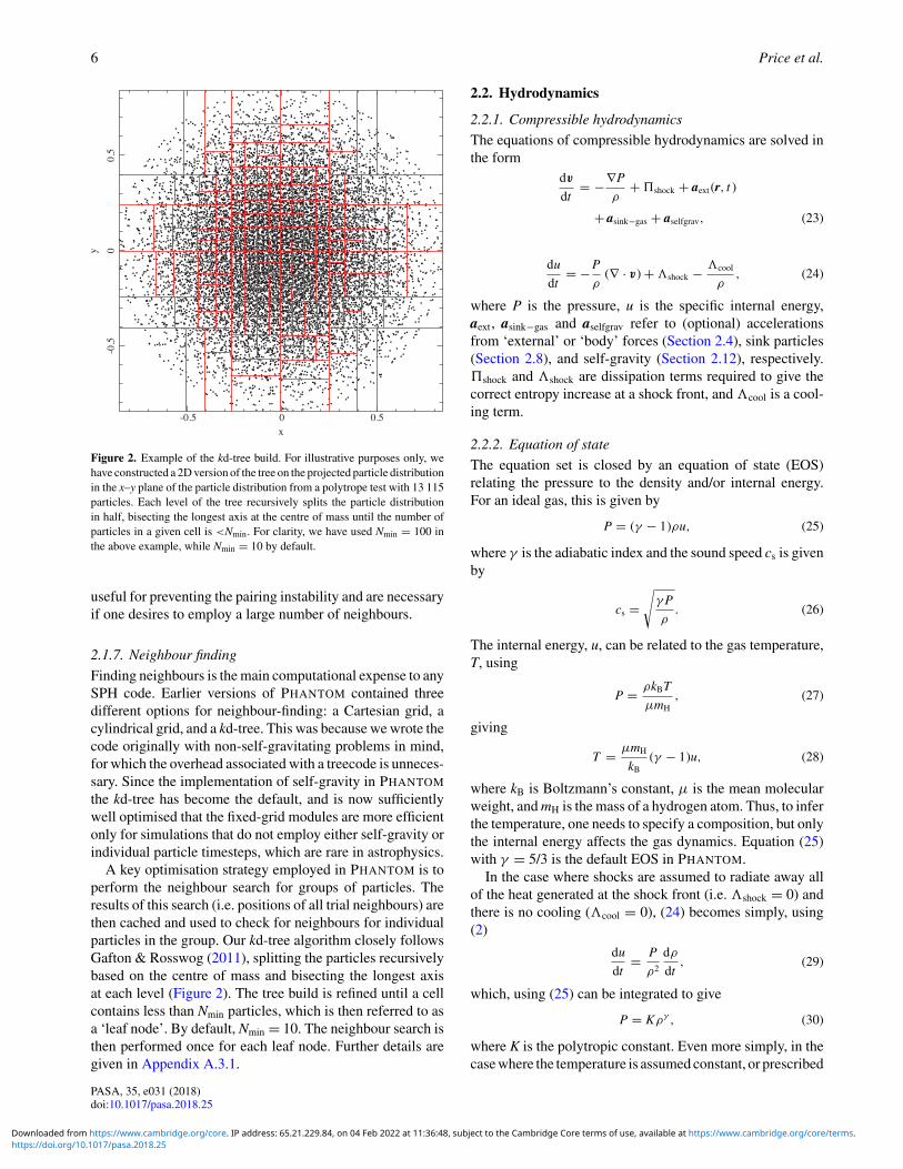
Figure 2. Example of the kd-tree build. For illustrative purposes only, wehave constructed a 2D version of the tree on the projected particle distributionin the x–y plane of the particle distribution from a polytrope test with 13 115particles. Each level of the tree recursively splits the particle distributionin half, bisecting the longest axis at the centre of mass until the number ofparticles in a given cell is <Nmin. For clarity, we have used Nmin = 100 inthe above example, while Nmin = 10 by default.

useful for preventing the pairing instability and are necessaryif one desires to employ a large number of neighbours.

2.1.7. Neighbour finding

Finding neighbours is the main computational expense to anySPH code. Earlier versions of PHANTOM contained threedifferent options for neighbour-finding: a Cartesian grid, acylindrical grid, and a kd-tree. This was because we wrote thecode originally with non-self-gravitating problems in mind,for which the overhead associated with a treecode is unneces-sary. Since the implementation of self-gravity in PHANTOM

the kd-tree has become the default, and is now sufficientlywell optimised that the fixed-grid modules are more efficientonly for simulations that do not employ either self-gravity orindividual particle timesteps, which are rare in astrophysics.

A key optimisation strategy employed in PHANTOM is toperform the neighbour search for groups of particles. Theresults of this search (i.e. positions of all trial neighbours) arethen cached and used to check for neighbours for individualparticles in the group. Our kd-tree algorithm closely followsGafton & Rosswog (2011), splitting the particles recursivelybased on the centre of mass and bisecting the longest axisat each level (Figure 2). The tree build is refined until a cellcontains less than Nmin particles, which is then referred to asa ‘leaf node’. By default, Nmin = 10. The neighbour search isthen performed once for each leaf node. Further details aregiven in Appendix A.3.1.

2.2. Hydrodynamics

2.2.1. Compressible hydrodynamics

The equations of compressible hydrodynamics are solved inthe form

dv

dt= −∇P

ρ+ shock + aext (r, t )

+ asink−gas + aselfgrav, (23)

du

dt= −P

ρ(∇ · v) + shock − cool

ρ, (24)

where P is the pressure, u is the specific internal energy,aext, asink−gas and aselfgrav refer to (optional) accelerationsfrom ‘external’ or ‘body’ forces (Section 2.4), sink particles(Section 2.8), and self-gravity (Section 2.12), respectively.shock and shock are dissipation terms required to give thecorrect entropy increase at a shock front, and cool is a cool-ing term.

2.2.2. Equation of state

The equation set is closed by an equation of state (EOS)relating the pressure to the density and/or internal energy.For an ideal gas, this is given by

P = (γ − 1)ρu, (25)

where γ is the adiabatic index and the sound speed cs is givenby

cs =√

γ P

ρ. (26)

The internal energy, u, can be related to the gas temperature,T, using

P = ρkBT

μmH, (27)

giving

T = μmH

kB(γ − 1)u, (28)

where kB is Boltzmann’s constant, μ is the mean molecularweight, and mH is the mass of a hydrogen atom. Thus, to inferthe temperature, one needs to specify a composition, but onlythe internal energy affects the gas dynamics. Equation (25)with γ = 5/3 is the default EOS in PHANTOM.

In the case where shocks are assumed to radiate away allof the heat generated at the shock front (i.e. shock = 0) andthere is no cooling (cool = 0), (24) becomes simply, using(2)

du

dt= P

ρ2

dρ

dt, (29)

which, using (25) can be integrated to give

P = Kργ , (30)

where K is the polytropic constant. Even more simply, in thecase where the temperature is assumed constant, or prescribed

PASA, 35, e031 (2018)doi:10.1017/pasa.2018.25






Phantom 7

as a function of position, the EOS is simply

P = c2s ρ. (31)

In both of these cases, (30) and (31), the internal energy doesnot need to be stored. In this case, the temperature is ef-fectively set by the value of K (and the density if γ �= 1).Specifically,

T = μmH

kBKργ−1. (32)

2.2.3. Code units

For pure hydrodynamics, physical units are irrelevant to thenumerical results since (1)–(2) and (23)–(24) are scale freeto all but the Mach number. Hence, setting physical units isonly useful when comparing simulations with Nature, whenphysical heating or cooling rates are applied via (24), or whenone wishes to interpret the results in terms of temperatureusing (28) or (32).

In the case where gravitational forces are applied, eitherusing an external force (Section 2.4) or using self-gravity(Section 2.12), we adopt the standard procedure of trans-forming units such that G = 1 in code units, i.e.

utime =√

u3dist

Gumass, (33)

where utime, udist, and umass are the units of time, length,and mass, respectively. Additional constraints apply whenusing relativistic terms (Section 2.4.5) or magnetic fields(Section 2.10.3).

2.2.4. Equation of motion in SPH

We follow the variable smoothing length formulation de-scribed by Price (2012a), Price & Federrath (2010), andLodato & Price (2010). We discretise (23) using

dva

dt= −

∑b

mb

[Pa + qa

ab

ρ2a�a

∇aWab(ha) + Pb + qbab

ρ2b�b

∇aWab(hb)

]

+ aext (ra, t ) + aasink−gas + aa

selfgrav, (34)

where the qaab and qb

ab terms represent the artificial viscosity(discussed in Section 2.2.7).

2.2.5. Internal energy equation

The internal energy equation (24) is discretised using the timederivative of the density sum (c.f. 29), which from (4) gives

dua

dt= Pa

ρ2a�a

∑b

mbvab · ∇aWab(ha) + shock − cool

ρ, (35)

where vab ≡ va − vb. In the variational formulation of SPH(e.g. Price 2012a), this expression is used as a constraint toderive (34), which guarantees both the conservation of energyand entropy (the latter in the absence of dissipation terms).The shock capturing terms in the internal energy equation arediscussed below.

By default, we assume an adiabatic gas, meaning that PdVwork and shock heating terms contribute to the thermal en-

ergy of the gas, no energy is radiated to the environment, andtotal energy is conserved. To approximate a radiative gas,one may set one or both of these terms to zero. Neglectingthe shock heating term, shock, gives an approximation equiv-alent to a polytropic EOS (30), as described in Section 2.2.2.Setting both shock and work contributions to zero impliesthat du/dt = 0, meaning that each particle will simply retainits initial temperature.

2.2.6. Conservation of energy in SPH

Does evolving the internal energy equation imply that totalenergy is not conserved? Wrong! Total energy in SPH, forthe case of hydrodynamics, is given by

E =∑

a

ma

(1

2v2

a + ua

). (36)

Taking the (Lagrangian) time derivative, we find that conser-vation of energy corresponds to

dE

dt=∑

a

ma

(va · dva

dt+ dua

dt

)= 0. (37)

Inserting our expressions (34) and (35), and neglecting forthe moment dissipative terms and external forces, we find

dE

dt= −

∑a

∑b

mamb

[Pavb

ρ2a�a

· ∇aWab(ha)

+ Pbva

ρ2b�b

· ∇aWab(hb)

]= 0. (38)

The double summation on the right-hand side equals zerobecause the kernel gradient, and hence the overall sum, isantisymmetric. That is, ∇aWab = −∇bWba. This means onecan relabel the summation indices arbitrarily in one half ofthe sum, and add it to one half of the original sum to givezero. One may straightforwardly verify that this remains truewhen one includes the dissipative terms (see below).

This means that even though we employ the internal en-ergy equation, total energy remains conserved to machineprecision in the spatial discretisation. That is, energy is con-served irrespective of the number of particles, the number ofneighbours or the choice of smoothing kernel. The only non-conservation of energy arises from the ordinary differentialequation solver one employs to solve the left-hand side ofthe equations. We thus employ a symplectic time integrationscheme in order to preserve the conservation properties asaccurately as possible (Section 2.3.1).

2.2.7. Shock capturing: momentum equation

The shock capturing dissipation terms are implemented fol-lowing Monaghan (1997), derived by analogy with Riemannsolvers from the special relativistic dissipation terms pro-posed by Chow & Monaghan (1997). These were extendedby Price & Monaghan (2004b, 2005) to MHD and recently todust–gas mixtures by Laibe & Price (2014b). In a recent pa-per, Puri & Ramachandran (2014) found this approach, alongwith the Morris & Monaghan (1997) switch (which they re-ferred to as the ‘Monaghan–Price–Morris’ formulation) to be

PASA, 35, e031 (2018)doi:10.1017/pasa.2018.25






8 Price et al.

the most accurate and robust method for shock capturing inSPH when compared to several other approaches, includingGodunov SPH (e.g. Inutsuka 2002; Cha & Whitworth 2003).

The formulation in PHANTOM differs from that given inPrice (2012a) only by the way that the density and signalspeed in the q terms are averaged, as described in Price &Federrath (2010) and Lodato & Price (2010). That is, weuse

ashock ≡ −

∑b

mb

[qa

ab

ρ2a�a

∇aWab(ha) + qbab

ρ2b�b

∇aWab(hb)

],

(39)where

qaab =

⎧⎨⎩−1

2ρavsig,avab · rab, vab · rab < 0

0 otherwise,(40)

where vab ≡ va − vb, rab ≡ (ra − rb)/|ra − rb| is the unitvector along the line of sight between the particles, and vsig

is the maximum signal speed, which depends on the physicsimplemented. For hydrodynamics, this is given by

vsig,a = αAVa cs,a + βAV|vab · rab|, (41)

where in general αAVa ∈ [0, 1] is controlled by a switch (see

Section 2.2.9), while βAV = 2 by default.Importantly, α does not multiply the βAV term. The βAV

term provides a second-order Von Neumann & Richtmyer-like term that prevents particle interpenetration (e.g. Lat-tanzio et al. 1986; Monaghan 1989), and thus βAV � 2 isneeded wherever particle penetration may occur. This is im-portant in accretion disc simulations where use of a low α

may be acceptable in the absence of strong shocks, but a lowβ will lead to particle penetration of the disc midplane, whichis the cause of a number of convergence issues (Meru & Bate2011, 2012). Price & Federrath (2010) found that βAV = 4was necessary at high Mach number (M � 5) to maintain asharp shock structure, which despite nominally increasing theviscosity was found to give less dissipation overall becauseparticle penetration no longer occurred at shock fronts.

2.2.8. Shock capturing: internal energy equation

The key insight from Chow & Monaghan (1997) was thatshock capturing not only involves a viscosity term but in-volves dissipating the jump in each component of the energy,implying a conductivity term in hydrodynamics and resistivedissipation in MHD (see Section 2.10.5). The resulting con-tribution to the internal energy equation is given by (e.g. Price2012a)

shock ≡ − 1

�aρa

∑b

mbvsig,a1

2(vab · rab)2Fab(ha)

+∑

b

mbαuvusig(ua − ub)

1

2

[Fab(ha)

�aρa+ Fab(hb)

�bρb

]

+ artres, (42)

where the first term provides the viscous shock heating, thesecond term provides an artificial thermal conductivity, Fab

is defined as in (15), and artres is the heating due to artifi-cial resistivity [Equation (182)]. The signal speed we use forconductivity term differs from the one used for viscosity, asdiscussed by Price (2008, 2012a). In PHANTOM, we use

vusig =

√|Pa − Pb|

ρab

(43)

for simulations that do not involve self-gravity or externalbody forces (Price 2008), and

vusig = |vab · rab| (44)

for simulations that do (Wadsley, Veeravalli, & Couchman2008). The importance of the conductivity term for treatingcontact discontinuities was highlighted by Price (2008), ex-plaining the poor results found by Agertz et al. (2007) in SPHsimulations of Kelvin–Helmholtz instabilities run across con-tact discontinuities (discussed further in Section 5.1.4). With(44), we have found there is no need for further switches to re-duce conductivity (e.g. Price 2004; Price & Monaghan 2005;Valdarnini 2016), since the effective thermal conductivity κ

is second order in the smoothing length (∝h2). PHANTOM

therefore uses αu = 1 by default in (42) and we have not yetfound a situation where this leads to excess smoothing.

It may be readily shown that the total energy remains con-served in the presence of dissipation by combining (42) withthe corresponding dissipative terms in (34). The contribu-tion to the entropy from both viscosity and conductivity isalso positive definite (see the appendix in Price & Monaghan2004b for the mathematical proof in the case of conductivity).

2.2.9. Shock detection

The standard approach to reducing dissipation in SPH awayfrom shocks for the last 15 yr has been the switch proposedby Morris & Monaghan (1997), where the dimensionless vis-cosity parameter α is evolved for each particle a accordingto

dαa

dt= max(−∇ · va, 0) − (αa − αmin )

τa, (45)

where τ ≡ h/(σ decayvsig) and σ decay = 0.1 by default. We setvsig in the decay time equal to the sound speed to avoid theneed to store dα/dt, since ∇ · v is already stored in order tocompute (4). This is the switch used for numerous turbulenceapplications with PHANTOM (e.g. Price & Federrath 2010;Price et al. 2011; Tricco et al. 2016b) where it is importantto minimise numerical dissipation in order to maximise theReynolds number (e.g. Valdarnini 2011; Price 2012b).

More recently, Cullen & Dehnen (2010) proposed a moreadvanced switch using the time derivative of the velocity di-vergence. A modified version based on the gradient of thevelocity divergence was also proposed by Read & Hayfield(2012). We implement a variation on the Cullen & Dehnen(2010) switch, using a shock indicator of the form

Aa = ξa max

[− d

dt(∇ · va ), 0

], (46)

PASA, 35, e031 (2018)doi:10.1017/pasa.2018.25






Phantom 9

where

ξ = |∇ · v|2|∇ · v|2 + |∇ × v|2 (47)

is a modification of the Balsara (1995) viscosity limiter forshear flows. We use this to set α according to

αloc,a = min

(10h2

aAa

c2s,a

, αmax

), (48)

where cs is the sound speed and αmax = 1. We use cs in theexpression for αloc also for MHD (Section 2.10) since wefound using the magnetosonic speed led to a poor treatmentof MHD shocks. If αloc, a > αa, we set αa = αloc, a, otherwisewe evolve αa according to

dαa

dt= − (αa − αloc,a)

τa, (49)

where τ is defined as in the Morris & Monaghan (1997) ver-sion, above. We evolve α in the predictor part of the inte-grator only, i.e. with a first-order time integration, to avoidcomplications in the corrector step. However, we perform thepredictor step implicitly using a backward Euler method, i.e.

αn+1a = αn

a + αloc,a�t/τa

1 + �t/τa, (50)

which ensures that the decay is stable regardless of thetimestep (we do this for the Morris & Monaghan methodalso).

We use the method outlined in Appendix B3 of Cullen& Dehnen (2010) to compute d(∇ · va)/dt . That is, we firstcompute the gradient tensors of the velocity, v, and accelera-tion, a (used from the previous timestep), during the densityloop using an SPH derivative operator that is exact to lin-ear order, that is, with the matrix correction outlined in Price(2004, 2012a), namely

Ri ja

∂vka

∂x ja

=∑

b

mb

(vk

b − vka

) ∂Wab(ha)

∂xi, (51)

where

Ri ja =

∑b

mb

(xi

b − xia

) ∂Wab(ha)

∂x j≈ δi j, (52)

and repeated tensor indices imply summation. Finally, weconstruct the time derivative of the velocity divergence ac-cording to

d

dt

(∂v i

a

∂xia

)= ∂ai

a

∂xia

− ∂v ia

∂x ja

∂v ja

∂xia

, (53)

where, as previously, repeated i and j indices imply summa-tion. In Cartesian coordinates, the last term in (53) can be

written out explicitly using

∂v ia

∂x ja

∂v ja

∂xia

=(

∂vx

∂x

)2

+(

∂vy

∂y

)2

+(

∂v z

∂z

)2

+ 2

[∂vx

∂y

∂vy

∂x+ ∂vx

∂z

∂v z

∂x+ ∂v z

∂y

∂vy

∂z

]. (54)

2.2.10. Cooling

The cooling term cool can be set either from detailed chem-ical calculations (Section 2.14.1) or, for discs, by the simple‘β-cooling’ prescription of Gammie (2001), namely

cool = ρu

tcool, (55)

where

tcool ≡ �(R)

βcool, (56)

with βcool an input parameter to the code specifying the cool-ing timescale in terms of the local orbital time. We compute� in (56) using � ≡ 1/(x2 + y2 + z2)3/2, i.e. assuming Keple-rian rotation around a central object with mass equal to unity,with G = 1 in code units.

2.2.11. Conservation of linear and angular momentum

The total linear momentum is given by

P =∑

a

mava, (57)

such that conservation of momentum corresponds to

dPdt

=∑

a

madva

dt= 0. (58)

Inserting our discrete equation (34), we find

dPdt

=∑

a

∑b

mamb

[Pa + qa

ab

ρ2a�a

∇aWab(ha)

+ Pb + qbab

ρ2b�b

∇aWab(hb)

]= 0, (59)

where, as for the total energy (Section 2.2.6), the double sum-mation is zero because of the antisymmetry of the kernelgradient. The same argument applies to the conservation ofangular momentum, ∑

a

mara × va (60)

(see e.g. Price 2012a for a detailed proof). As with total en-ergy, this means linear and angular momentum are exactlyconserved by our SPH scheme to the accuracy with whichthey are conserved by the timestepping scheme.

In PHANTOM, linear and angular momentum are both con-served to round-off error (typically ∼10−16 in double pre-cision) with global timestepping, but exact conservation isviolated when using individual particle timesteps or whenusing the kd-tree to compute gravitational forces. The mag-nitude of these quantities, as well as the total energy and theindividual components of energy (kinetic, internal, potential,

PASA, 35, e031 (2018)doi:10.1017/pasa.2018.25






10 Price et al.

and magnetic), should thus be monitored by the user at run-time. Typically with individual timesteps, one should expectenergy conservation to �E/E ∼ 10−3 and linear and angularmomentum conservation to ∼10−6 with default code settings.The code execution is aborted if conservation errors exceed10%.

2.3. Time integration

2.3.1. Timestepping algorithm

We integrate the equations of motion using a generalisation ofthe Leapfrog integrator which is reversible in the case of bothvelocity dependent forces and derivatives which depend onthe velocity field. The basic integrator is the Leapfrog methodin ‘Kick–Drift–Kick’ or ‘Velocity Verlet’ form (Verlet 1967),where the positions and velocities of particles are updatedfrom time tn to tn + 1 according to

vn+ 12 = vn + 1

2�tan, (61)

rn+1 = rn + �tvn+ 12 , (62)

an+1 = a(rn+1), (63)

vn+1 = vn+ 12 + 1

2�tan+1, (64)

where �t ≡ tn + 1 − tn. This is identical to the formulation ofLeapfrog used in other astrophysical SPH codes (e.g. Springel2005; Wadsley et al. 2004). The Verlet scheme, being bothreversible and symplectic (e.g. Hairer, Lubich, & Wanner2003), preserves the Hamiltonian nature of the SPH algo-rithm (e.g. Gingold & Monaghan 1982b; Monaghan & Price2001). In particular, both linear and angular momentum areexactly conserved, there is no long-term energy drift, andphase space volume is conserved (e.g. for orbital dynamics).In SPH, this is complicated by velocity-dependent terms inthe acceleration from the shock-capturing dissipation terms.In this case, the corrector step, (64), becomes implicit. Theapproach we take is to notice that these terms are not usuallydominant over the position-dependent terms. Hence, we usea first-order prediction of the velocity, as follows:

vn+ 12 = vn + 1

2�tan, (65)

rn+1 = rn + �tvn+ 12 , (66)

v∗ = vn+ 12 + 1

2�tan, (67)

an+1 = a(rn+1, v∗), (68)

vn+1 = v∗ + 1

2�t[an+1 − an

]. (69)

At the end of the step, we then check if the error in the first-order prediction is less than some tolerance ε according to

e = |vn+1 − v∗||vmag| < εv, (70)

where vmag is the mean velocity on all SPH particles (we setthe error to zero if |vmag| = 0) and by default εv = 10−2.If this criterion is violated, then we recompute the acceler-ations by replacing v∗ with vn+1 and iterating (68) and (69)until the criterion in (70) is satisfied. In practice, this happensrarely, but occurs for example in the first few steps of the Se-dov problem where the initial conditions are discontinuous(Section 5.1.3). As each iteration is as expensive as halvingthe timestep, we also constrain the subsequent timestep suchthat iterations should not occur, i.e.

�t = min

(�t,

�t√emax/ε

), (71)

where emax = max (e) over all particles. A caveat to the aboveis that velocity iterations are not currently implemented whenusing individual particle timesteps.

Additional variables such as the internal energy, u, andthe magnetic field, B, are timestepped with a predictor andtrapezoidal corrector step in the same manner as the velocity,following (65), (67) and (69).

Velocity-dependent external forces are treated separately,as described in Section 2.4.

2.3.2. Timestep constraints

The timestep itself is determined at the end of each step, andis constrained to be less than the maximum stable timestep.For a given particle, a, this is given by (e.g. Lattanzio et al.1986; Monaghan 1997)

�tC,a ≡ Ccourha

vdtsig,a

, (72)

where Ccour = 0.3 by default (Lattanzio et al. 1986) and vdtsig is

taken as the maximum of (41) over the particle’s neighboursassuming αAV = max (αAV, 1). The criterion above differsfrom the usual Courant–Friedrichs–Lewy condition used inEulerian codes (Courant, Friedrichs, & Lewy 1928) becauseit depends only on the difference in velocity between neigh-bouring particles, not the absolute value.

An additional constraint is applied from the accelerations(the ‘force condition’), where

�tf,a ≡ Cforce

√ha

|aa| , (73)

where Cforce = 0.25 by default. A separate timestep constraintis applied for external forces

�text,a ≡ Cforce

√h

|aext,a| , (74)

PASA, 35, e031 (2018)doi:10.1017/pasa.2018.25






Phantom 11

and for accelerations to SPH particles to/from sink particles(Section 2.8)

�tsink−gas,a ≡ Cforce

√ha

|asink−gas,a| . (75)

For external forces with potentials defined such that � → 0as r → ∞, an additional constraint is applied using (Dehnen& Read 2011)

�t�,a ≡ Cforceη�

√|�a|

|∇�|2a, (76)

where η� = 0.05 (see Section 2.8.5).The timestep for particle a is then taken to be the minimum

of all of the above constraints, i.e.

�ta = min(�tC, �tf , �text, �tsink−gas, �t�

)a, (77)

with possible other constraints arising from additionalphysics as described in their respective sections. With globaltimestepping, the resulting timestep is the minimum over allparticles

�t = mina

(�ta). (78)

2.3.3. Substepping of external forces

In the case where the timestep is dominated by any of theexternal force timesteps, i.e. (74)–(76), we implement an op-erator splitting approach implemented according to the re-versible reference system propagator algorithm (RESPA) de-rived by Tuckerman, Berne, & Martyna (1992) for moleculardynamics. RESPA splits the acceleration into ‘long-range’and ‘short-range’ contributions, which in PHANTOM are de-fined to be the SPH and external/point-mass accelerations,respectively.

Our implementation follows Tuckerman et al. (1992) (seetheir Appendix B), where the velocity is first predicted tothe half step using the ‘long-range’ forces, followed by aninner loop where the positions are updated with the currentvelocity and the velocities are updated with the ‘short-range’accelerations. Thus, the timestepping proceeds according to

v = v + �tsph

2an

sph, (79)

v = v + �text

2am

ext, (80)

r = r + �textv, (81)

get aext (r), (82)

v = v + �text

2am+1

ext , (83)

over substeps

⎧⎪⎪⎪⎪⎪⎪⎪⎪⎪⎨⎪⎪⎪⎪⎪⎪⎪⎪⎪⎩

get asph(r), (84)

v = v + �tsph

2an

sph, (85)

where asph indicates the SPH acceleration evaluated from(34) and aext indicates the external forces. The SPH and

external accelerations are stored separately to enable this.�text is the minimum of all timesteps relating to sink–gasand external forces [equations (74)–(76)], while �tsph is thetimestep relating to the SPH forces [equations (72), (73), and(288)]. �text is allowed to vary on each substep, so we takeas many steps as required such that

∑m−1j �text, j + �text, f =

�tsph, where �text, f < �text, j is chosen so that the sumwill identically equal �tsph. The number of substeps is m≈ int(�text, min/�tsph, min) + 1, where the minimum is takenover all particles.

2.3.4. Individual particle timesteps

For simulations of stiff problems with a large range intimestep over the domain, it is more efficient to allow eachparticle to evolve on its own timestep independently (Bate1995; Springel 2005; Saitoh & Makino 2010). This violatesall of the conservation properties of the Leapfrog integra-tor [see Makino et al. (2006) for an attempt to solve this],but can speed up the calculation by an order of magnitudeor more. We implement this in the usual blockstepped man-ner by assigning timesteps in factor-of-two decrements fromsome maximum timestep �tmax, which for convenience is setequal to the time between output files.

We implement a timestep limiter where the timestep foran active particle is constrained to be within a factor of 2of its neighbours, similar to condition employed by Saitoh &Makino (2009). Additionally, inactive particles will be wokenup as required to ensure that their timestep is within a factorof 2 of its neighbours.

The practical side of individual timestepping is describedin Appendix A.6.

2.4. External forces

2.4.1. Point-mass potential

The simplest external force describes a point mass, M, at theorigin, which yields gravitational potential and acceleration:

�a = −GM

ra, aext,a = −∇�a = − GM

|ra|3 ra, (86)

where ra ≡ |ra| ≡ √ra · ra. When this potential is used, we

allow for particles within a certain radius, Racc, from the originto be accreted. This allows for a simple treatment of accretiondiscs where the mass of the disc is assumed to be negligiblecompared to the mass of the central object. The accreted massin this case is recorded but not added to the central mass. Formore massive discs, or when the accreted mass is significantwith respect to the central mass, it is better to model thecentral star using a sink particle (Section 2.8) where there aremutual gravitational forces between the star and the disc, andany mass accreted is added to the point mass (Section 2.8.2).

2.4.2. Binary potential

We provide the option to model motion in binary systemswhere the mass of the disc is negligible. In this case, the

PASA, 35, e031 (2018)doi:10.1017/pasa.2018.25






12 Price et al.

binary motion is prescribed using

r1 = [(1 − M ) cos(t ), (1 − M ) sin(t ), 0], (87)

r2 = [−M cos(t ),−M sin(t ), 0], (88)

where M is the mass ratio in units of the total mass (which istherefore unity). For this potential, G and � are set to unityin computational units, where � is the angular velocity of thebinary. Thus, only M needs to be specified to fix both m1 andm2. Hence, the binary remains fixed on a circular orbit at r =1. The binary potential is therefore

�a = − M

|ra − r1| − (1 − M )

|ra − r2| , (89)

such that the external acceleration is given by

aext,a = −∇�a = −M(ra − r1)

|ra − r1|3 − (1 − M )(ra − r2)

|ra − r2|3 . (90)

Again, there is an option to accrete particles that fall within acertain radius from either star (Racc, 1 or Racc, 2, respectively).For most binary accretion disc simulations (e.g. planet migra-tion), it is better to use ‘live’ sink particles to represent the bi-nary so that there is feedback between the binary and the disc(we have used a live binary in all of our simulations to date,e.g. Nixon, King, & Price 2013; Facchini, Lodato, & Price2013; Martin et al. 2014a, 2014b; Dogan et al. 2015; Ragusa,Lodato, & Price 2016; Ragusa et al. 2017), but the binary po-tential remains useful under limited circumstances—in par-ticular, when one wishes to turn off the feedback between thedisc and the binary.

Given that the binary potential is time-dependent, for ef-ficiency, we compute the position of the binary only once atthe start of each timestep, and use these stored positions tocompute the accelerations of the SPH particles via (90).

2.4.3. Binary potential with gravitational wave decay

An alternative binary potential including the effects of grav-itational wave decay was used by Cerioli, Lodato, & Price(2016) to study the squeezing of discs during the merger ofsupermassive black holes. Here the motion of the binary isprescribed according to

r1 =[− m2

m1 + m2a cos(θ ),− m2

m1 + m2a sin(θ ), 0

],

r2 =[

m1

m1 + m2a cos(θ ),

m1

m1 + m2a sin(θ ), 0

], (91)

where the semi-major axis, a, decays according to

a(t ) = a0

(1 − t

τ

) 14

. (92)

The initial separation is a0, with τ defined as the time tomerger, given by the usual expression (e.g. Lodato et al.2009)

τ ≡ 5

256

a40

μ12(m1 + m2)2, (93)

where

μ12 ≡ m1m2

m1 + m2. (94)

The angle θ is defined using

� ≡ dθ

dt=√

G(m1 + m2)

a3. (95)

Inserting the expression for a and integrating gives (Cerioliet al. 2016)

θ (t ) = −8τ

5

√G(m1 + m2)

a30

(1 − t

τ

). (96)

The positions of the binary, r1 and r2, can be inserted into(89) to obtain the binary potential, with the acceleration asgiven in (90). The above can be used as a simple example ofa time-dependent external potential.

2.4.4. Galactic potentials

We implement a range of external forces representing vari-ous galactic potentials, as used in Pettitt et al. (2014). Theseinclude arm, bar, halo, disc, and spheroidal components. Werefer the reader to the paper above for the actual forms of thepotentials.

For the non-axisymmetric potentials, a few important pa-rameters that determine the morphology can be changed atrun time rather than compile time. These include the patternspeed, arm number, arm pitch angle, and bar axis lengths(where applicable). In the case of non-axisymmetric compo-nents, the user should be aware that some will add mass tothe system, whereas others simply perturb the galactic disc.These potentials can be used for any galactic system, but thevarious default scale lengths and masses are chosen to matchthe Milky Way’s rotation curve (Sofue 2012).

The most basic potential in PHANTOM is a simple loga-rithmic potential from Binney & Tremaine (1987), which al-lows for the reproduction of a purely flat rotation curve withsteep decrease at the galactic centre, and approximates thehalo, bulge, and disc contributions. Also included is the stan-dard flattened disc potential of Miyamoto–Nagai (Miyamoto& Nagai 1975) and an exponential profile disc, specificallythe form from Khoperskov et al. (2013). Several spheroidalcomponents are available, including the potentials of Plum-mer (1911), Hernquist (1990), and Hubble (1930). These canbe used generally for bulges and halos if given suitable massand scale lengths. We also include a few halo-specific pro-files; the NFW (Navarro, Frenk, & White 1996), Begeman,Broeils, & Sanders (1991), Caldwell & Ostriker (1981), andthe Allen & Santillan (1991) potentials.

The arm potentials include some of the more complicatedprofiles. The first is the potential of Cox & Gómez (2002),which is a relatively straightforward superposition of threesinusoidal-based spiral components to damp the potential‘troughs’ in the inter-arm minima. The other spiral poten-tial is from Pichardo et al. (2003), and is more complicated.Here, the arms are constructed from a superposition of oblatespheroids whose loci are placed along a standard logarithmic

PASA, 35, e031 (2018)doi:10.1017/pasa.2018.25






Phantom 13

spiral. As the force from this potential is computationally ex-pensive it is prudent to pre-compute a grid of potential/forceand read it at run time. The python code to generate the ap-propriate grid files is distributed with the code.

Finally, the bar components: We include the bar potentialsof Dehnen (2000a), Wada & Koda (2001), the ‘S’ shaped barof Vogt & Letelier (2011), both biaxial and triaxial versionsprovided in Long & Murali (1992), and the boxy-bulge barof Wang et al. (2012). This final bar contains both a small in-ner non-axisymmetric bulge and longer bar component, withthe forces calculated by use of Hernquist–Ostriker expansioncoefficients of the bar density field. PHANTOM contains thecoefficients for several different forms of this bar potential.

2.4.5. Lense–Thirring precession

Lense–Thirring precession (Lense & Thirring 1918) froma spinning black hole is implemented in a post-Newtonianapproximation following Nelson & Papaloizou (2000), whichhas been used in Nixon et al. (2012b), Nealon, Price, & Nixon(2015), and Nealon et al. (2016). In this case, the externalacceleration consists of a point-mass potential (Section 2.4.1)and the Lense–Thirring term:

aext,a = −∇�a + va × �p,a, (97)

where �a is given by (86) and va × �p,a is the gravitomag-netic acceleration. A dipole approximation is used, yielding

�p,a ≡ 2S|ra|3 − 6(S · ra)ra

|ra|5 , (98)

with S = aspin(GM )2k/c3, where k is a unit vector in the di-rection of the black hole spin. When using the Lense–Thirringforce, geometric units are assumed such that G = M = c =1, as described in Section 2.2.3, but with the additional con-straints on the unit system from M and c.

Since in this case the external force depends on velocity, itcannot be implemented directly into Leapfrog. The methodwe employ to achieve this is simpler than those proposedelsewhere [c.f. attempts by Quinn et al. (2010) and Rein &Tremaine (2011) to adapt the Leapfrog integrator to Hill’sequations]. Our approach is to split the acceleration into po-sition and velocity-dependent parts, i.e.

aext = aext,x(r) + aext,v(r, v). (99)

The position-dependent part [i.e. −∇�(r)] is integratedas normal. The velocity-dependent Lense–Thirring term isadded to the predictor step, (66)–(67), as usual, but the cor-rector step, (69), is written in the form

vn+1 = vn+ 12 + 1

2�t[an+1

sph + an+1ext,x + aext,v(rn+1, vn+1)

], (100)

where vn+ 12 ≡ vn + 1

2�tan as in (65). This equation is im-plicit but the trick is to notice that it can be solved analyticallyfor simple forces4. In the case of Lense–Thirring precession,

4 The procedure for Hill’s equations would be identical to our method forLense–Thirring precession. The method we use is both simpler and moredirect than any of the schemes proposed by Quinn et al. (2010) and Rein

we have

vn+1 = v + 1

2�t[vn+1 × �p(rn+1)

], (101)

where v ≡ vn+ 12 + 1

2�t (an+1sph + an+1

ext,x). We therefore have amatrix equation in the form

Rvn+1 = v, (102)

where R is the 3 × 3 matrix given by

R ≡

⎡⎢⎢⎢⎢⎢⎢⎣

1 −�t

2�z

p

�t

2�y

p

�t

2�z

p 1 −�t

2�x

p

−�t

2�y

p

�t

2�x

p 1

⎤⎥⎥⎥⎥⎥⎥⎦

. (103)

Rearranging (102), vn+1 is obtained by using

vn+1 = R−1v, (104)

where R−1 is the inverse of R, which we invert using theanalytic solution.

2.4.6. Generalised Newtonian potential

The generalised Newtonian potential described by Tejeda& Rosswog (2013) is implemented, where the accelerationterms are given by

aext,a = −GMra

|ra|3 f 2 + 2Rgva(va · ra)

|ra|3 f− 3Rgra(va × ra )2

|ra|5 ,

(105)with Rg ≡ GM/c3 and f ≡ (

1 − 2Rg/|ra|). See Bonnerot et al.

(2016) for a recent application. This potential reproduces sev-eral features of the Schwarzschild (1916) spacetime, in par-ticular, reproducing the orbital and epicyclic frequencies tobetter than 7% (Tejeda & Rosswog 2013). As the acceler-ation involves velocity-dependent terms, it requires a semi-implicit solution like Lense–Thirring precession. Since thematrix equation is rather involved for this case, the correctorstep is iterated using fixed point iterations until the velocityof each particle is converged to a tolerance of 1%.

2.4.7. Poynting–Robertson drag

The radiation drag from a central point-like, gravitating, radi-ating, and non-rotating object may be applied as an externalforce. The implementation is intended to be as general as pos-sible. The acceleration of a particle subject to these externalforces is

aext,a = (k0βPR − 1)GM

|ra|3 ra

−βPR

(k1

GM

|ra|3vr

cra − k2

GM

|ra|2va

c

), (106)

where vr is the component of the velocity in the radial di-rection. The parameter βPR is the ratio of radiation to grav-itational forces, supplied by a separate user-written module.

& Tremaine (2011), and is time reversible unlike the methods proposed inthose papers.

PASA, 35, e031 (2018)doi:10.1017/pasa.2018.25






14 Price et al.

Relativistic effects are neglected because these are thought tobe less important than radiation forces for low (βPR < 0.01)luminosities, even in accreting neutron star systems wherea strong gravitational field is present (e.g., Miller & Lamb1993).

The three terms on the right side of (106) correspond, re-spectively, to gravity (reduced by outward radiation pres-sure), redshift-related modification to radiation pressurecaused by radial motion, and Poynting–Robertson dragagainst the direction of motion. These three terms can bescaled independently by changing the three parameters k0,k1, and k2, whose default values are unity. Rotation of thecentral object can be crudely emulated by changing k2.

As for Lense–Thirring precession, the an+1 term of theLeapfrog integration scheme can be expanded into velocity-dependent and non-velocity-dependent component. We ob-tain, after some algebra,

vn+1 = −T − Qk1(vn+1 · r)r1 + Qk2

, (107)

where

T = vn + 1

2�tan − (1 − k0βPR )GM�t

2r3r (108)

and

Q = GMβPR�t

2cr2. (109)

Equation (107) yields a set of simultaneous equations for thethree vector components that can be solved analytically. Adetailed derivation is given in Worpel (2015).

2.4.8. Coriolis and centrifugal forces

Under certain circumstances, it is useful to perform calcu-lations in a co-rotating reference frame (e.g. for dampingbinary stars into equilibrium with each other). The resultingacceleration terms are given by

aext,a = −� × (� × ra) − 2(� × va ), (110)

which are the centrifugal and Coriolis terms, respectively,with � the angular rotation vector. The timestepping algo-rithm is as described above for Lense–Thirring precession,with the velocity-dependent term handled by solving the 3 ×3 matrix in the Leapfrog corrector step.

2.5. Driven turbulence

PHANTOM implements turbulence driving in periodic do-mains via an Ornstein–Uhlenbeck stochastic driving of theacceleration field, as first suggested by Eswaran & Pope(1988). This is an SPH adaptation of the module used in thegrid-based simulations by Schmidt, Hillebrandt, & Niemeyer(2006) and Federrath, Klessen, & Schmidt (2008) and manysubsequent works. This module was first used in PHAN-TOM by Price & Federrath (2010) to compare the statis-tics of isothermal, supersonic turbulence between SPH, andgrid methods. Subsequent applications have been to the den-sity variance–Mach number relation (Price et al. 2011), sub-

sonic turbulence (Price 2012b), supersonic MHD turbulence(Tricco et al. 2016b), and supersonic turbulence in a dust–gas mixture (Tricco et al. 2017). Adaptations of this modulehave also been incorporated into other SPH codes (Bauer &Springel 2012; Valdarnini 2016).

The amplitude and phase of each Fourier mode is initialisedby creating a set of six random numbers, zn, drawn from arandom Gaussian distribution with unit variance. These aregenerated by the usual Box–Muller transformation (e.g. Presset al. 1992) by selecting two uniform random deviates u1, u2

∈ [0, 1] and constructing the amplitude according to

z =√

2 log(1/u1) cos(2πu2). (111)

The six Gaussian random numbers are set up according to

xn = σ zn, (112)

where the standard deviation, σ , is set to the square rootof the energy per mode divided by the correlation time,σ = √

Em/tdecay, where both Em and tdecay are user-specifiedparameters.

The ‘red noise’ sequence (Uhlenbeck & Ornstein 1930)is generated for each mode at each timestep according to(Bartosch 2001)

xn+1 = f xn + σ√

(1 − f 2)zn, (113)

where f = exp ( − �t/tdecay) is the damping factor. The re-sulting sequence has zero mean with root-mean-square equalto the variance. The power spectrum in the time domain canvary from white noise [P(f) constant] to ‘brown noise’ [P(f)= 1/f2].

The amplitudes and phases of each mode are constructedby splitting xn into two vectors, �a and �b of length 3, em-ployed to construct divergence- and curl-free fields accordingto

Am = w[�a − (�a · k)k] + (1 − w)[(�b · k)k], (114)

Bm = w[�b − (�b · k)k] + (1 − w)[(�a · k)k], (115)

where k = [kx, ky, kz] is the mode frequency. The parame-ter w ∈ [0, 1] is the ‘solenoidal weight’, specifying whetherthe driving should be purely solenoidal (w = 1) or purelycompressive (w = 0) (see Federrath et al. 2008, 2010a).

The spectral form of the driving is defined in Fourier space,with options for three possible spectral forms

Cm =

⎧⎪⎪⎪⎨⎪⎪⎪⎩

1 uniform

4(amin − 1)(k − kc )2

(kmax − kmin )2+ 1 parabolic

k/k−5/3min Kolmogorov,

(116)

where k =√

k2x + k2

y + k2z is the wavenumber, with non-zero

amplitudes defined only for wavenumbers where kmin � k �kmax , and amin is the amplitude of the modes at kmin and kmax

in the parabolic case (we use amin = 0 in the code). The fre-quency grid is defined using frequencies from kx = nx2π /Lx

PASA, 35, e031 (2018)doi:10.1017/pasa.2018.25






Phantom 15

in the x direction, where nx ∈ [0, 20] is an integer and Lx isthe box size in the x-direction, while ky = ny2π /Ly and kz =nz2π /Lz with ny ∈ [0, 8] and nz ∈ [0, 8]. We then set up fourmodes for each combination of nx, ny, and nz, correspondingto [kx, ky, kz], [kx, −ky, kz], [kx, ky, −kz], and [kx, −ky, −kz].That is, we effectively sum from [− (N − 1)/2, (N − 1)/2]in the ky and kz directions in the discrete Fourier transform,where N = max (nx) is the number of frequencies. The defaultvalues for kmin and kmax are 2π and 6π , respectively, corre-sponding to large-scale driving of only the first few Fouriermodes, so with default settings there are 112 non-zero Fouriermodes. The maximum number of modes, defining the arraysizes needed to store the stirring information, is currently setto 1,000.

We apply the forcing to the particles by computing thediscrete Fourier transform over the stirring modes directly,i.e.

aforcing,a = fsol

nmodes∑m=1

Cm [Am cos(k · ra ) − Bm sin(k · ra)] , (117)

where the factor fsol is defined from the solenoidal weight, w,according to

fsol =√

3

ndim

√3

1 − 2w + ndimw2, (118)

such that the rms acceleration is the same irrespective of thevalue of w. We default to purely solenoidal forcing (w =1), with the factor fsol thus equal to

√3/2 by default. For

individual timesteps, we update the driving force only whena particle is active.

To aid reproducibility, it is often desirable to pre-generatethe entire driving sequence prior to performing a calculation,which can then be written to a file and read back at runtime.This was the procedure used in Price & Federrath (2010),Tricco et al. (2016b), and Tricco et al. (2017).

2.6. Accretion disc viscosity

Accretion disc viscosity is implemented in PHANTOM viatwo different approaches, as described by Lodato & Price(2010).

2.6.1. Disc viscosity using the shock viscosity term

The default approach is to adapt the shock viscosity term torepresent a Shakura & Sunyaev (1973) α-viscosity, as orig-inally proposed by Artymowicz & Lubow (1994) and Mur-ray (1996). The key is to note that (39) and (40) represent aNavier–Stokes viscosity term with a fixed ratio between thebulk and shear viscosity terms (e.g. Murray 1996; Jubelgas,Springel, & Dolag 2004; Lodato & Price 2010; Price 2012b;Meru & Bate 2012). In particular, it can be shown (e.g. Es-pañol & Revenga 2003) that

∑b

mb

ρab

(vab · rab)∇aWab

|rab| ≈ 1

5∇ (∇ · v) + 1

10∇2v, (119)

where ρab is some appropriate average of the density. Thisenables the artificial viscosity term, (39), to be translated intothe equivalent Navier–Stokes terms. In order for the artificialviscosity to represent a disc viscosity, we make the followingmodifications (Lodato & Price 2010):

1. The viscosity term is applied for both approaching andreceding particles.

2. The speed v sig is set equal to cs.3. A constant αAV is adopted, turning off shock detection

switches (Section 2.2.9).4. The viscosity term is multiplied by a factor h/|rab|.

The net result is that (40) becomes

qaab =

⎧⎨⎩− ρaha

2|rab|(αAVcs,a + βAV|vab · rab|

)vab · rab, vab · rab < 0

− ρaha2|rab|α

AVcs,avab · rab. otherwise.(120)

With the above modifications, the shear and bulk coeffi-cients can be translated using (119) to give (e.g. Monaghan2005; Lodato & Price 2010; Meru & Bate 2012)

νAV ≈ 1

10αAVcsh, (121)

ζAV = 5

3νAV ≈ 1

6αAVcsh. (122)

The Shakura–Sunyaev prescription is

ν = αSScsH, (123)

where H is the scale height. This implies that αSS may bedetermined from αAV using

αSS ≈ αAV

10

〈h〉H

, (124)

where 〈h〉 is the mean smoothing length on particles in acylindrical ring at a given radius.

In practice, this means that one must uniformly resolvethe scale height in order to obtain a constant αSS in the disc.We have achieved this in simulations to date by choosingthe initial surface density profile and the power-law indexof the temperature profile (when using a locally isothermalEOS) to ensure that this is the case (Lodato & Pringle 2007).Confirmation that the scaling provided by (124) is correct isshown in Figure 4 of Lodato & Price (2010) and is checkedautomatically in the PHANTOM test suite.

In the original implementation (Lodato & Price 2010), wealso set the βAV to zero, but this is dangerous if the disc dy-namics are complex as there is nothing to prevent particlepenetration (see Section 2.2.7). Hence, in the current versionof the code, βAV = 2 by default even if disc viscosity is set,but is only applied to approaching particles (c.f. 120). Apply-ing any component of viscosity to only approaching particlescan affect the sign of the precession induced in warped discs(Lodato & Pringle 2007), but in general retaining the βAV

PASA, 35, e031 (2018)doi:10.1017/pasa.2018.25






16 Price et al.

term is safer with no noticeable effect on the overall dissi-pation due to the second-order dependence of this term onresolution.

Using αAV to set the disc viscosity has two useful conse-quences. First, it forces one to consider whether or not thescale height, H, is resolved. Second, knowing the value ofαAV is helpful, as αAV ≈ 0.1 represents the lower bound be-low which a physical viscosity is not resolved in SPH (that is,viscosities smaller than this produce disc spreading indepen-dent of the value of αAV, see Bate 1995; Meru & Bate 2012),while αAV > 1 constrains the timestep (Section 2.3.2).

2.6.2. Disc viscosity using the Navier–Stokes viscosityterms

An alternative approach is to compute viscous terms directlyfrom the Navier–Stokes equation. Details of how the Navier–Stokes terms are represented are given below (Section 2.7),but for disc viscosity a method for determining the kinematicviscosity is needed, which in turn requires specifying thescale height as a function of radius. We use

Ha ≡ cas

�(Ra), (125)

where we assume Keplerian rotation � =√

GM/R3 and cs

is obtained for a given particle from the EOS (which forconsistency must be either isothermal or locally isothermal).It is important to note that this restricts the application of thisapproach only to discs where R can be meaningfully defined,excluding, for example, discs around binary stars.

The shear viscosity is then set using

νa = αSScas Ha, (126)

where αSS is a pre-defined/input parameter. The timestep isconstrained using Cvisch2/ν as described in Section 2.7. Theadvantage to this approach is that the shear viscosity is setdirectly and does not depend on the smoothing length. How-ever, as found by Lodato & Price (2010), it remains necessaryto apply some bulk viscosity to capture shocks and preventparticle penetration of the disc midplane, so one should ap-ply the shock viscosity as usual. Using a shock-detectionswitch (Section 2.2.9) means that this is usually not prob-lematic. This formulation of viscosity was used in Facchiniet al. (2013).

2.7. Navier–Stokes viscosity

Physical viscosity is implemented as described in Lodato &Price (2010). Here, (23) and (24) are replaced by the com-pressible Navier–Stokes equations, i.e.

dv i

dt= − 1

ρ

∂Si jNS

∂x j+ shock + aext (r, t )

+ asink−gas + aselfgrav, (127)

du

dt= −P

ρ(∇ · v) + visc + shock − cool

ρ, (128)

with the stress tensor given by

Si jNS =

[P −

(ζ − 2

3η

)∂vk

∂xk

]δi j − η

(∂v i

∂x j+ ∂v j

∂xi

), (129)

where δij is the Kronecker delta, and ζ and η are the bulkand shear viscosity coefficients, related to the volume andkinematic shear viscosity coefficients by ζ v ≡ ζ /ρ and ν ≡η/ρ.

2.7.1. Physical viscosity using two first derivatives

As there is no clear consensus on the best way to implementphysical viscosity in SPH, PHANTOM currently contains twoimplementations. The simplest is to use two first derivatives,which is essentially that proposed by Flebbe et al. (1994),Watkins et al. (1996), and Sijacki & Springel (2006). In thiscase, (127) is discretised in the standard manner using

dv ia

dt= −

∑b

mb

[Si j

NS,a

�aρ2a

∂Wab(ha)

∂x ja

+ Si jNS,b

�bρ2b

∂Wab(hb)

∂x ja

]

+ ishock + ai

ext (r, t ) + aisink−gas + ai

selfgrav, (130)

where the velocity gradients are computed during the densityloop using

∂v ia

∂x ja

= − 1

�aρa

∑b

mbviab∇ j

aWab(ha). (131)

Importantly, the differenced SPH operator is used in (131),whereas (130) uses the symmetric gradient operator. The useof conjugate operators5 is a common requirement in SPH inorder to guarantee energy conservation and a positive defi-nite entropy increase from dissipative terms (e.g. Price 2010;Tricco & Price 2012). Total energy conservation means that

dE

dt=∑

a

ma

(dua

dt+ v i

a

dv ia

dt

)= 0. (132)

This implies a contribution to the thermal energy equationgiven by

dua

dt= Si j

NS,a

�aρ2a

∑b

mbviab∇ j

aWab(ha), (133)

which can be seen to reduce to (24) in the inviscid case (Si jNS =

Pδi j), but in general is an SPH expression for

dua

dt= −Si j

NS,a

ρa

∂v ia

∂x ja

. (134)

Using Si jNS = S ji

NS, we have

dua

dt= −1

2

Si jNS,a

ρa

(∂v i

a

∂x ja

+ ∂v ja

∂xia

), (135)

which, using (129), gives

visc =(

ζv,a − 2

3νa

)(∇ · v)2

a + νa

2

(∂v i

a

∂x ja

+ ∂v ja

∂xia

)2

. (136)

5 The SPH difference operator is discretely skew adjoint to the symmetricoperator (Cummins & Rudman 1999).

PASA, 35, e031 (2018)doi:10.1017/pasa.2018.25






Phantom 17

By the square in the last term, we mean the tensor summa-tion �j�iTijTij, where Ti j ≡ ∂v i

a/∂x ja + ∂v j

a/∂xia. The heat-

ing term is therefore positive definite provided that the veloc-ity gradients and divergence are computed using the differ-ence operator (131), both in (136) and when computing thestress tensor (129).

The main disadvantage of the first derivatives approach isthat it requires storing the strain tensor for each particle, i.e.six additional quantities when taking account of symmetries.

2.7.2. Physical viscosity with direct second derivatives

The second approach is to use SPH second derivative opera-tors directly. Here we use modified versions of the identitiesgiven by Español & Revenga (2003) (see also Monaghan2005; Price 2012a), namely

∇ [A(∇ · v)] ≈

−∑

b

mb

[Aa

ρaGab(ha) + Ab

ρbGab(hb)

](vab · rab)rab, (137)

∇ · (C∇v) ≈ −∑

b

mb

[Ca

ρaGab(ha) + Cb

ρbGab(hb)

]vab, (138)

where Gab ≡ −2Fab/|rab|, i.e. the scalar part of the kernel gra-dient divided by the particle separation, which can be thoughtof as equivalent to defining a new ‘second derivative kernel’(Brookshaw 1985, 1994; Price 2012a; Price & Laibe 2015a).

From the compressible Navier–Stokes equations, (127)with (129), the coefficients in these two terms are

A ≡ 1

2

(ζ + η

3

), (139)

C ≡ 1

2η, (140)

so that we can simply use(dv i

a

dt

)visc

=∑

b

mb

[τa

ρaGab(ha) + τb

ρbGab(hb)

](vab · rab)ri

ab

+∑

b

mb

[κa

ρaGab(ha ) + κb

ρbGab(hb)

]v i

ab (141)

where

τ = 5

2A, (142)

κ =(

C − A

2

). (143)

The corresponding heating terms in the thermal energyequation are given by

visc = τa

ρa

∑b

mb(vab · rab)2Gab(ha )

+ κa

ρa

∑b

mb(vab)2Gab(ha ). (144)

This is the default formulation of Navier–Stokes viscosityin the code since it does not require additional storage. In

practice, we have found little difference between the two for-mulations of physical viscosity, but this would benefit froma detailed study. In general one might expect the two firstderivatives formulation to offer a less noisy estimate at thecost of additional storage. However, direct second derivativesare the method used in ‘Smoothed Dissipative Particle Dy-namics’ (Español & Revenga 2003).

2.7.3. Timestep constraint

Both approaches to physical viscosity use explicit timestep-ping, and therefore imply a constraint on the timestep givenby

�t avisc ≡ Cvisc

h2a

νa, (145)

where Cvisc = 0.25 by default (Brookshaw 1994). When phys-ical viscosity is turned on, this constraint is included withother timestep constraints according to (77).

2.7.4. Physical viscosity and the tensile instability

Caution is required in the use of physical viscosity at highMach number, since negative stress can lead to the tensile in-stability (Morris 1996b; Monaghan 2000; Gray, Monaghan,& Swift 2001). For subsonic applications, this is usually nota problem since the strain tensor and velocity divergence aresmall compared to the pressure. In the current code, we sim-ply emit a warning if physical viscosity leads to negativestresses during the calculation, but this would benefit from adetailed study.

2.7.5. Physical viscosity and angular momentumconservation

Neither method for physical viscosity exactly conserves an-gular momentum because the force is no longer directed alongthe line of sight joining the particles. However, the error isusually small (see discussion in Bonet & Lok 1999, Section 5of Price & Monaghan 2004b or Hu & Adams 2006). Recently,Müller, Fedosov, & Gompper (2015) have proposed an algo-rithm for physical viscosity in SPH that explicitly conservesangular momentum by tracking particle spin, which may beworth investigating.

2.8. Sink particles

Sink particles were introduced into SPH by Bate, Bonnell,& Price (1995) in order to follow star formation simula-tions beyond the point of fragmentation. In PHANTOM, theseare treated separately to the SPH particles, and interact withother particles, including other sink particles, only via grav-ity. The differences with other point-mass particles imple-mented in the code (e.g. dust, stars, and dark matter) are

PASA, 35, e031 (2018)doi:10.1017/pasa.2018.25






18 Price et al.

that (i) the gravitational interaction is computed using a di-rect N2 summation which is not softened by default (i.e.,the N-body algorithm is collisional); (ii) they are allowed toaccrete gas; and (iii) they store the accreted angular momen-tum and other extended properties, such as the accreted mass.Sink particles are evolved in time using the RESPA algorithm(Section 2.3.3), which is second-order accurate, symplectic,and allows sink particles to evolve on shorter timesteps com-pared to SPH particles.

2.8.1. Sink particle accelerations

The equations of motion for a given sink particle, i, are

dvi

dt= −

Nsink∑j=1

GMjφ′i j (ε)ri j

−Npart∑b=1

Gmbφ′ib(εib)rib, (146)

where φ′ab is the softening kernel (Section 2.12.2), Npart is the

total number of gas particles, and Nsink is the total number ofsink particles. The sink–gas softening length, εib, is definedas the maximum of the (fixed) softening length defined forthe sink particles, ε, and the softening length of the gas par-ticle, εb. That is, εib ≡ max (ε, εb). SPH particles receive acorresponding acceleration

aasink−gas = −

Nsink∑j=1

GMjφ′a j (εa j )ra j . (147)

Softening of sink–gas interactions is not applied if the soft-ening length for sink particles is set to zero, in which case thesink–gas accelerations reduce simply to

aasink−gas = −

Nsink∑j=1

GMj

|ra − r j |3 ra j . (148)

This is the default behaviour when sink particles are usedin the code. Softening of sink–gas interactions is useful tomodel a point-mass particle that does not accrete gas (e.g. bysetting the accretion radius to zero). For example, we used asoftened sink particle to simulate the core of the red giant inIaconi et al. (2017). The sink–sink interaction is unsoftenedby default (ε = 0), giving the usual

aisink−sink = −

Nsink∑j=1

GMj

|ri − r j |3 ri j . (149)

Caution is required when integrating tight binary or multiplesystems when ε = 0 to ensure that the timestep conditions(Section 2.3.2) are strict enough.

2.8.2. Accretion onto sink particles

Accretion of gas particles onto a sink particle occurs whena gas particle passes a series of accretion checks within theaccretion radius racc of a sink particle (set in the initial condi-tions or when the sink particle is created, see Section 2.8.4).

First, a gas particle is indiscriminately accreted without un-dergoing any additional checks if it falls within faccracc, where0� facc � 1 (default facc = 0.8). In the boundary region faccracc

< r < racc, a gas particle undergoes accretion if

1. |Lai| < |Lacc|, that is, its specific angular momentum isless than that of a Keplerian orbit at racc,

2. e = v2ai2 − GMi

rai< 0, i.e., it is gravitationally bound to the

sink particle, and3. e for this gas–sink pair is smaller than e with any other

sink particle, that is, out of all sink particles, the gasparticle is most bound to this one.

In the above conditions, Lai is the relative specific angularmomentum of the gas–sink pair, a − i, defined by

|L2ai| ≡ |rai × vai|2

= r2aiv

2ai − (rai · vai )

2 , (150)

while |Lacc| = r2acc�acc is the angular momentum at racc,

where �acc =√

GMi/r3ai is the Keplerian angular speed at

racc, vai, and rai are the relative velocity and position, respec-tively, and Mi is the mass of the sink particle.

When a particle, a, passes the accretion checks, then themass, position, velocity, acceleration, and spin angular mo-mentum of the sink particle are updated according to

ri = (rama + riMi )

Mi + ma, (151)

vi = (vama + viMi )

Mi + ma, (152)

ai = (aama + aiMi )

Mi + ma, (153)

Si = Si + maMi

Mi + ma[(ra − ri ) × (va − vi )] , (154)

Mi = Mi + ma. (155)

This ensures that mass, linear momentum, and angular mo-mentum (but not energy) are conserved by the accretion pro-cess. The accreted mass as well as the total mass for eachsink particle is stored to avoid problems with round-off errorin the case where the particle masses are much smaller thanthe sink mass. Accreted particles are tagged by setting theirsmoothing lengths negative. Those particles with h � 0 aresubsequently excluded when the kd-tree is built.

2.8.3. Sink particle boundary conditions

No special sink particle boundary conditions are imple-mented in PHANTOM at present. More advanced boundaryconditions to regularise the density, pressure, and angular mo-mentum near a sink have been proposed by Bate et al. (1995)and used in Bate & Bonnell (1997), and proposed again more

PASA, 35, e031 (2018)doi:10.1017/pasa.2018.25






Phantom 19

recently by Hubber, Walch, & Whitworth (2013b). Whilethese conditions help to regularise the flow near the sink par-ticle, they can also cause problems—particularly the angularmomentum boundary condition if the disc near the sink par-ticle has complicated structure such as spiral density waves(Bate 2014, private communication). Often it is more costeffective to simply reduce the accretion radius of the sink.This may change in future code versions.

2.8.4. Dynamic sink particle creation

As described in Bate et al. (1995), it is also possible to createsink particles on-the-fly provided certain physical conditionsare met and self-gravity is turned on (Section 2.12). The pri-mary conditions required for sink particle formation are thatthe density of a given particle exceeds some threshold phys-ical density somewhere in the domain, and that this densitypeak occurs more than a critical distance rcrit from an existingsink. Once these conditions are met on a particular particle,a, the creation of a new sink particle occurs by passing thefollowing conditions (Bate et al. 1995):

1. The particle is a gas particle.2. ∇ · va ≤ 0, that is, gas surrounding the particle is at rest

or collapsing.3. ha < racc/2, i.e., the smoothing length of the particle is

less than half of the accretion radius.4. All neighbours within racc are currently active.5. The ratio of thermal to gravitational energy of particles

within racc, αJ, satisfies αJ � 1/2.6. αJ + βrot � 1, where βrot = |erot|/|egrav| is the ratio of

rotational energy to the magnitude of the gravitationalenergy for particles within racc.

7. etot < 0, that is, the total energy of particles within racc

is negative (i.e. the clump is gravitationally bound).8. The particle is at a local potential minimum, i.e. � is

less than � computed on all other particles within racc

(Federrath et al. 2010b).

A new sink particle is created at the position of particlea if these checks are passed, and immediately the particleswithin racc are accreted by calling the routine described inSection 2.8.2. The checks above are the same as those inBate et al. (1995), with the additional check from Federrathet al. (2010b) to ensure that sink particles are only created ina local minimum of the gravitational potential.

The various energies used to evaluate the criteria above arecomputed according to

ekin = 1

2

N<racc∑b=1

mb(vb − va)2, (156)

etherm =N<racc∑

b=1

mbub, (157)

egrav = −1

2

N<racc∑b=1

N<racc∑c=b

Gmbmc,

× [φ(|rb − rc|, hb) + φ(|rb − rc|, hc )] , (158)

etot = ekin + etherm + egrav, (159)

erot ≡√

e2rot,x + e2

rot,y + e2rot,z, (160)

erot,x ≡ 1

2

N<racc∑b=1

mb

L2ab,x√

(ya − yb)2 + (za − zb)2, (161)

erot,y ≡ 1

2

N<racc∑b=1

mb

L2ab,y√

(xa − xb)2 + (za − zb)2, (162)

erot,z ≡ 1

2

N<racc∑b=1

mb

L2ab,z√

(xa − xb)2 + (ya − yb)2, (163)

where Lab ≡ (ra − rb) × (va − vb) is the specific angularmomentum between a pair of particles, and φ is the grav-itational softening kernel (defined in Section 2.12), whichhas units of inverse length. Adding the contribution from allpairs, b − c, within the clump is required to obtain the totalpotential of the clump.

2.8.5. Sink particle timesteps

Sink particles are integrated together with a global, but adap-tive, timestep, following the inner loop of the RESPA al-gorithm given in (80)–(83) corresponding to a second-orderLeapfrog integration. The timestep is controlled by the mini-mum of the sink–gas timestep, (75), and a sink–sink timestep(Dehnen & Read 2011)

�tsink−sink ≡ mini

(Cforceη�

√|�sink−sink

i ||∇�sink−sink

i |2)

, (164)

where the potential and gradient include other sink particles,plus any external potentials applied to sink particles exceptthe sink–gas potential. We set η� = 0.05 by default, resultingin ∼300–500 steps per orbit for a binary orbit with the defaultCforce = 0.25 (see Section 5.5.1).

More accurate integrators such as the fourth-order Her-mite scheme (Makino & Aarseth 1992) or the fourth-ordersymplectic schemes proposed by Omelyan, Mryglod, & Folk(2002) or Chin & Chen (2005) are not yet implemented in

PASA, 35, e031 (2018)doi:10.1017/pasa.2018.25






20 Price et al.

PHANTOM, but it would be a worthwhile effort to incorpo-rate one of these in a future code version. See Hubber et al.(2013a) for a recent implementation of a fourth-order Her-mite scheme for sink particles in SPH.

2.9. Stellar physics

A tabulated EOS can be used to take account of the departurefrom an ideal gas, for example, due to changes in ionisa-tion or molecular dissociation and recombination. This tab-ulated EOS in PHANTOM is adapted from the log Pgas − TEOS tables provided with the open source package Modulesfor Experiments in Stellar Astrophysics MESA (Paxton et al.2011). Details of the data, originally compiled from blendsof equations of state from Saumon, Chabrier, & van Horn(1995) (SCVH), Timmes & Swesty (2000), Rogers & Nay-fonov (2002, also the 2005 update), Potekhin & Chabrier(2010) and for an ideal gas, are outlined by Paxton et al.(2011).

In our implementation (adapted from original routines forthe MUSIC code; Goffrey et al. 2017), we compute the pres-sure and other required EOS variables for a particular com-position by interpolation between sets of tables for differenthydrogen abundance X = 0.0, 0.2, 0.4, 0.6, 0.8 and metallic-ity Z = 0.0, 0.02, 0.04. Pressure is calculated with bicubicinterpolation, and �1 ≡ ∂ln P/∂lnρ|s with bilinear interpola-tion, in log u and log V ≡ logρ − 0.7log u + 20. The tablesare currently valid in the ranges 10.5 � log u � 17.5 and0.0 � log V � 14.0. Values requested outside the tables arecurrently computed by linear extrapolation. This triggers awarning to the user.

We have not tested the thermodynamic consistency ofour interpolation scheme from the tables (Timmes & Arnett1999).

2.10. Magnetohydrodynamics

PHANTOM implements the smoothed particle magnetohydro-dynamics (SPMHD) algorithm described in Price (2012a)and Tricco & Price (2012, 2013), based on the original workby Phillips & Monaghan (1985) and Price & Monaghan(2004a, 2004b, 2005). PHANTOM was previously used to testa vector potential formulation (Price 2010), but this algorithmhas been subsequently removed from the code due to its poorperformance (see Price 2010).

The important difference between PHANTOM and theGADGET implementation of SPMHD (Dolag & Stasyszyn2009; Bürzle et al. 2011a, 2011b), which also implementsthe core algorithms from Price & Monaghan (2004a, 2004b,2005), is our use of the divergence-cleaning algorithm fromTricco & Price (2012, 2013) and Tricco, Price, & Bate(2016a). This is vital for preserving the divergence-free (nomonopoles) condition on the magnetic field.

For recent applications of PHANTOM to MHD problems,see e.g. Tricco et al. (2016b), Dobbs et al. (2016), Bonnerot

et al. (2017), Forgan, Price, & Bonnell (2017), and Wursteret al. (2016, 2017).

2.10.1. Equations of magnetohydrodynamics

PHANTOM solves the equations of MHD in the form

dv i

dt= − 1

ρ

∂Mi j

∂x j+ shock + f i

divB + aiext

+ aisink−gas + ai

selfgrav, (165)

du

dt= −P

ρ(∇ · v) + shock − cool

ρ, (166)

d

dt

(Bρ

)= 1

ρ[(B · ∇ ) v − ∇ψ + Ddiss] , (167)

d

dt

(ψ

ch

)= −ch (∇ · B) − 1

2

ψ

ch(∇ · v) − ψ

chτc, (168)

where B is the magnetic field, ψ is a scalar used tocontrol the divergence error in the magnetic field (seeSection 2.10.8), and Ddiss represents magnetic dissipationterms (Sections 2.10.5 and 2.11). The Maxwell stress ten-sor, Mij, is given by

Mi j =(

P + 1

2

B2

μ0

)δi j − BiB j

μ0, (169)

where δij is the Kronecker delta and μ0 is the permeability offree space. A source term related to the numerically induceddivergence of the magnetic field, given by

f idivB ≡ −Bi

ρ(∇ · B) (170)

is necessary to prevent the tensile instability in SPMHD(Phillips & Monaghan 1985; Monaghan 2000; Børve,Omang, & Trulsen 2001; Price 2012a). With this source term,the equation set for ideal MHD in the absence of the diver-gence cleaning field, ψ , is formally the same as in the Powellet al. (1999) eight-wave scheme (Price 2012a), meaning thatthe divergence errors in the magnetic field are advected bythe flow, but not dissipated, unless cleaning is used.

2.10.2. Discrete equations

The discrete version of (165) follows the same procedure asfor physical viscosity (Section 2.7), i.e.

dv ia

dt= −

∑b

mb

[Mi j

a

�aρ2a

∂Wab(ha)

∂x ja

+ Mi jb

�bρ2b

∂Wab(hb)

∂x ja

]

+ ashock + f i

divB,a + aiext,a + ai

sink−gas

+ aiselfgrav, (171)

where Mi ja is defined according to (169), fdivB is a correction

term for stability (discussed below), and accelerations due toexternal forces are as described in Section 2.4.

PASA, 35, e031 (2018)doi:10.1017/pasa.2018.25






Phantom 21

Equations (167) and (168) are discretised according to(Price & Monaghan 2005; Tricco & Price 2012; Tricco et al.2016a)

d

dt

(Bρ

)a

= − 1

�aρ2a

∑b

mbvab [Ba · ∇aWab(ha)]

−∑

b

mb

[ψa

�aρ2a

∇aWab(ha ) + ψb

�bρ2b

∇aWab(hb)

]

+ 1

ρaDa

diss, (172)

d

dt

(ψ

ch

)a

= cah

�aρa

∑b

mbBab · ∇aWab(ha)

+ ψa

2cah�aρa

∑b

mbvab · ∇aWab(ha) − ψa

cahτ

ac

. (173)

The first term in (173) uses the divergence of the magneticfield discretised according to

(∇ · B)a = − 1

�aρa

∑b

mb (Ba − Bb) · ∇aWab(ha), (174)

which is therefore the operator we use when measuring thedivergence error (c.f. Tricco & Price 2012).

2.10.3. Code units

An additional unit is required when magnetic fields are in-cluded to describe the unit of magnetic field. We adopt codeunits such that μ0 = 1, as is common practice. The unit scal-ings for the magnetic field can be determined from the defi-nition of the Alfvén speed,

vA ≡√

B2

μ0ρ. (175)

Since the Alfvén speed has dimensions of length per unittime, this implies a unit for the magnetic field, umag, givenby

umag =(

μ0umass

udistutime

) 12

. (176)

Converting the magnetic field in the code to physical unitstherefore only requires specifying μ0 in the relevant unit sys-tem. In particular, it avoids the differences between SI andcgs units in how the charge unit is defined, since μ0 is dimen-sionless and equal to 4π in cgs units but has dimensions thatinvolve charge in SI units.

2.10.4. Tensile instability correction

The correction term fdivB is necessary to avoid the tensileinstability—a numerical instability where particles attracteach other along field lines—in the regime where the mag-netic pressure exceeds the gas pressure, that is, when plasmaβ ≡ P/ 1

2 B2 < 1 (Phillips & Monaghan 1985). The correctionterm is computed using the symmetric divergence operator

(Børve et al. 2001; Price 2012a; Tricco & Price 2012)

f idivB,a = −Bi

a

∑b

mb

[Ba · ∇aWab(ha)

�aρ2a

+ Bb · ∇aWab(hb)

�bρ2b

]. (177)

Since this term violates momentum conservation to the extentthat the ∇ · B term is non-zero, several authors have proposedways to minimise its effect. Børve et al. (2004) showed thatstability could be achieved with Bi = 1

2 Bi and also proposeda scheme for scaling this term to zero for β > 1. Barnes,Kawata, & Wu (2012) similarly advocated using a factor of12 in this term. However, Tricco & Price (2012) showed thatthis could lead to problematic effects (their Figure 12). InPHANTOM, we use

Bi =⎧⎨⎩

Bi β < 2,

[(10 − β )Bi]/8 2 < β < 10,

0 otherwise(178)

to provide numerical stability in the strong field regime whilemaintaining conservation of momentum when β > 10. Thisalso helps to reduce errors in the MHD wave speed causedby the correction term (Iwasaki 2015).

2.10.5. Shock capturing

The shock capturing term in the momentum equation forMHD is identical to (39) and (40) except that the signal speedbecomes (Price & Monaghan 2004a, 2005; Price 2012a)

vsig,a = αAVa va + βAV|vab · rab|, (179)

where

va =√

c2s,a + v2

A,a (180)

is the fast magnetosonic speed. Apart from this, the majordifference to the hydrodynamic case is the addition of anartificial resistivity term to capture shocks and discontinuitiesin the magnetic field (i.e. current sheets). This is given by

Dadiss = ρa

2

∑b

mb

[vB

sig,a

ρ2a

Fab(ha)

�a+ vB

sig,b

ρ2b

Fab(hb)

�b

]Bab, (181)

where vBsig,a is an appropriate signal speed (see below) multi-

plied by a dimensionless coefficient, αB. The correspondingcontribution to the thermal energy from the resistivity termin (42) is given by

artres = −1

4

∑b

mb

[vB

sig,a

ρ2a

Fab(ha)

�a

+ vBsig,b

ρ2b

Fab(hb)

�b

](Bab)2. (182)

As with the artificial viscosity, (181) and (182) are the SPHrepresentation of a physical resistivity term, η∇2B, but witha coefficient that is proportional to resolution (Price & Mon-aghan 2004a). The resistive dissipation rate from the shock

PASA, 35, e031 (2018)doi:10.1017/pasa.2018.25






22 Price et al.

capturing term is given by

η ≈ 1

2αBvB

sig|rab|, (183)

where |rab|∝h.

2.10.6. Switch to reduce resistivity

PHANTOM previously used the method proposed by Tricco& Price (2013) to reduce the dissipation in the magnetic fieldaway from shocks and discontinuities. The signal velocity,vB

sig, was set equal to the magnetosonic speed [Equation (180)]multiplied by the dimensionless coefficient αB, which was setaccording to

αBa = min

(ha

|∇Ba||Ba| , αB

max

), (184)

where αBmax = 1.0 by default and |∇Ba| is the two-norm of

the gradient tensor, i.e. the root mean square of all nine com-ponents of this tensor. Unlike the viscous dissipation, this isset based on the instantaneous values of h and B and there isno source/decay equation involved, as Tricco & Price (2013)found it to be unnecessary. Since αB is proportional to reso-lution, from (183), we see that this results in dissipation thatis effectively second order (∝h2). When individual particletimesteps were used, inactive particles retained their value ofαB from the last timestep they were active.

More recently, we have found that a better approach, sim-ilar to that used for artificial conductivity, is to simply setαB = 1 for all particles and set the signal speed for artificialresistivity according to

vBsig = |vab × rab|. (185)

We find that this produces better results on all of our tests(Section 5.6), in particular, producing zero numerical dissipa-tion on the current loop advection test (Section 5.6.5). As withthe Tricco & Price (2013) switch, it gives second-order dis-sipation in the magnetic field (demonstrated in Section 5.6.1,Figure 26). This is now the default treatment for artificialresistivity in PHANTOM.

2.10.7. Conservation properties

The total energy when using MHD is given by

E =∑

a

ma

(1

2v2

a + ua + �a + 1

2

B2a

μ0ρa

). (186)

Hence, total energy conservation, in the absence of diver-gence cleaning, corresponds to

dE

dt=∑

a

ma

[va · dva

dt+ dua

dt+ d�a

dt

+ B2a

2μ0ρ2a

dρa

dt+ Ba

μ0· d

dt

(Bρ

)a

]= 0. (187)

Neglecting the fdivB correction term for the moment, substitut-ing (171), (35), and (172) into (187) with the ideal MHD andshock capturing terms included demonstrates that the totalenergy is exactly conserved, using the same argument as the

one given in Section 2.2.6 (detailed workings can be foundin Price & Monaghan 2004b). The total linear momentumis also exactly conserved following a similar argument as inSection 2.2.11. However, the presence of the fdivB correctionterm, though necessary for numerical stability, violates theconservation of both momentum and energy in the strong fieldregime (in the weak field regime, it is switched off and con-servation is preserved). The severity of this non-conservationis related to the degree in which divergence errors are presentin the magnetic field, hence inadequate divergence control(see below) usually manifests as a loss of momentum con-servation in the code (see Tricco & Price 2012, for details).

2.10.8. Divergence cleaning

We adopt the ‘constrained’ hyperbolic/parabolic divergencecleaning algorithm described by Tricco & Price (2012) andTricco et al. (2016a) to preserve the divergence-free conditionon the magnetic field. This formulation addresses a numberof issues with earlier formulations by Dedner et al. (2002)and Price & Monaghan (2005).

The main idea of the scheme is to propagate divergenceerrors according to a damped wave equation (Dedner et al.2002; Price & Monaghan 2005). This is facilitated by intro-ducing a new scalar field, ψ , which is coupled to the magneticfield in (167) and evolved according to (168).

Tricco et al. (2016a) generalised the method of Dedneret al. (2002) to include the case where the hyperbolic wavespeed, ch, varies in time and space. This is the approach weuse in PHANTOM. The resulting ‘generalised wave equation’may be derived by combining the relevant term in (167) with(168) to give (Tricco et al. 2016a)

d

dt

[1√ρch

d

dt

(ψ√ρch

)]− ∇2ψ

ρ

+ d

dt

[1√ρch

(ψ√ρchτc

)]= 0. (188)

When ch, ρ, τ c, and the fluid velocity are constant, this re-duces to the usual damped wave equation in the form

∂2ψ

∂t2− c2

h∇2ψ + 1

τc

∂ψ

∂t= 0. (189)

The same equation holds for the evolution of ∇ · B itself, i.e.

∂2(∇ · B)

∂t2− c2

h∇2(∇ · B) + 1

τc

∂ (∇ · B)

∂t= 0, (190)

from which it is clear that ch represents the speed at whichdivergence errors are propagated and τ c is the decay timescaleover which divergence errors are removed.

Tricco & Price (2012) formulated a ‘constrained’ SPMHDimplementation of hyperbolic/parabolic cleaning whichguarantees numerical stability of the cleaning. The constraintimposed by Tricco & Price (2012) is that, in the absence ofdamping, any energy removed from the magnetic field duringcleaning must be conserved by the scalar field, ψ . This en-forces particular choices of numerical operators for ∇ · B and∇ψ in (172) and (173), respectively, in particular that they

PASA, 35, e031 (2018)doi:10.1017/pasa.2018.25






Phantom 23

form a conjugate pair of difference and symmetric derivativeoperators. This guarantees that the change of magnetic en-ergy is negative definite in the presence of the parabolic term(see below).

In PHANTOM, we set the cleaning speed, ch, equal to thefast magnetosonic speed [Equation (180)] so that its timestepconstraint is satisfied already by (72), as recommended byTricco & Price (2013). The decay timescale is set accordingto

τ ac ≡ ha

σcch,a, (191)

where the dimensionless factor σ c sets the ratio of parabolicto hyperbolic cleaning. This is set to σ c = 1.0 by default,which was empirically determined by Tricco & Price (2012)to provide optimal reduction of divergence errors in threedimensions.

The divergence cleaning dissipates energy from the mag-netic field at a rate given by (Tricco & Price 2012)

(dE

dt

)cleaning

= −∑

a

maψ2

a

μ0ρac2h,aτ

ac

. (192)

In general, this is so small compared to other dissipation terms(e.g. resistivity for shock capturing) that it is not worth moni-toring (Tricco et al. 2016a). This energy is not added as heat,but simply removed from the calculation.

2.10.9. Monitoring of divergence errors andover-cleaning

The divergence cleaning algorithm is guaranteed to eitherconserve or dissipate magnetic energy, and cleans divergenceerrors to a sufficient degree for most applications. However,the onus is on the user to ensure that divergence errors arenot affecting simulation results. This may be monitored bythe dimensionless quantity

εdivB ≡ h|∇ · B||B| . (193)

The maximum and mean values of this quantity should beused to check the fidelity of simulations that include magneticfields. A good rule-of-thumb is that the mean should remain� 10−2 for the simulation to remain qualitatively unaffectedby divergence errors.

The cleaning wave speed can be arbitrarily increased to im-prove the effectiveness of the divergence cleaning accordingto

ch,a = fcleanva, (194)

where fclean is an ‘over-cleaning’ factor (by default, fclean =1, i.e. no ‘over-cleaning’). Tricco et al. (2016a) showed thatincreasing fclean leads to further reduction in divergence er-rors, without affecting the quality of obtained results, but withan accompanying computational expense associated with areduction in the timestep size.

2.11. Non-ideal magnetohydrodynamics

PHANTOM implements non-ideal MHD including terms forOhmic resistivity, ambipolar (ion-neutral) diffusion and theHall effect. Algorithms and tests are taken from Wurster,Price, & Ayliffe (2014) and Wurster, Price, & Bate (2016).See Wurster et al. (2016, 2017) and Wurster, Bate, & Price(2018) for recent applications. Our formulation of non-idealSPMHD in PHANTOM is simpler than the earlier formula-tion proposed by Hosking & Whitworth (2004) because weconsider only one set of particles, representing a mixture ofcharged and uncharged species. Ours is similar to the imple-mentation by Tsukamoto, Iwasaki, & Inutsuka (2013) andTsukamoto et al. (2015).

2.11.1. Equations of non-ideal MHD

We assume the strong coupling or ‘heavy ion’ approxima-tion (see e.g. Wardle & Ng 1999; Shu et al. 2006; Pandey &Wardle 2008), which neglects ion pressure and assumes ρ i

� ρn, where the subscripts i and n refer to the ionised andneutral fluids, respectively. In this case, (167) contains threeadditional terms in the form

d

dt

(Bρ

)nimhd

= − 1

ρ∇ ×

[Jσe

+ J × Bene

− (J × B) × BγADρi

],

(195)where σ e is the electrical conductivity, ne is the number den-sity of electrons, e is the charge on an electron, and γ AD isthe collisional coupling constant between ions and neutrals(Pandey & Wardle 2008). We write this in the form

d

dt

(Bρ

)nimhd

= − 1

ρ∇ ×

[ηOJ + ηHJ × B

− ηAD(J × B) × B], (196)

where B is the unit vector in the direction of B such thatηO, ηAD, and ηHall are the coefficients for resistive and am-bipolar diffusion and the Hall effect, respectively, each withdimensions of area per unit time.

To conserve energy, we require the corresponding resistiveand ambipolar heating terms in the thermal energy equationin the form

(du

dt

)nimhd

= ηO

ρJ2 + ηAD

ρ

[J2 − (J · B)2

]. (197)

The Hall term is non-dissipative, being dispersive rather thandiffusive, so does not enter the energy equation.

We currently neglect the ‘Biermann battery’ term (Bier-mann 1950) proportional to ∇Pe/(ene) in our non-ideal MHDimplementation, both because it is thought to be negligiblein the interstellar medium (Pandey & Wardle 2008) and be-cause numerical implementations can produce incorrect re-sults (Graziani et al. 2015). This term is mainly importantin generating seed magnetic fields for subsequent dynamoprocesses (e.g. Khomenko et al. 2017).

PASA, 35, e031 (2018)doi:10.1017/pasa.2018.25






24 Price et al.

2.11.2. Discrete equations

Our main constraint is that the numerical implementation ofthe non-ideal MHD terms should exactly conserve energy,which is achieved by discretising in the form (Wurster et al.2014)

d

dt

(Bρ

)nimhd,a

= −∑

b

⎡⎣ Da

�aρ2a

× ∇aWab(ha)

+ Db

�bρ2b

× ∇aWab(hb)

⎤⎦, (198)

where

D = −ηOJ − ηH(J × B) + ηAD[(J × B) × B]. (199)

The corresponding term in the energy equation is given by(dua

dt

)nimhd

= −Da · Ja

ρa, (200)

where the magnetic current density is computed alongsidethe density evaluation according to

J = 1

�aρa

∑b

mb(Ba − Bb) × ∇aWab(ha). (201)

Non-ideal MHD therefore utilises a ‘two first derivatives’approach, similar to the formulation of physical viscosity de-scribed in Section 2.7.1. This differs from the ‘direct secondderivatives’ approach used for our artificial resistivity term,and in previous formulations of physical resistivity (Bonafedeet al. 2011). In practice, the differences are usually minor. Ourmain reason for using two first derivatives for non-ideal MHDis that it is easier to incorporate the Hall effect and ambipolardiffusion terms.

2.11.3. Computing the non-ideal MHD coefficients

To self-consistently compute the coefficients ηO, ηH, andηAD from the local gas properties, we use the NICIL library(Wurster 2016) for cosmic ray ionisation chemistry and ther-mal ionisation. We refer the reader to Wurster (2016) andWurster et al. (2016) for details, since this is maintained andversioned as a separate package.

2.11.4. Timestepping

With explicit timesteps, the timestep is constrained in a sim-ilar manner to other terms, using

�t = Cnimhdh2

max(ηO, ηAD, |ηH|) , (202)

where Cnimhd = 1/(2π ) by default. This can prove prohibitive,so we employ the so-called ‘super-timestepping’ algorithmfrom Alexiades, Amiez, & Gremaud (1996) to relax the sta-bility criterion for the Ohmic and ambipolar terms (only). Theimplementation is described in detail in Wurster et al. (2016).Currently, the Hall effect is always timestepped explicitly inthe code.

2.12. Self-gravity

PHANTOM includes self-gravity between particles. By self-gravity, we mean a solution to Poisson’s equation

∇2� = 4πGρ(r), (203)

where � is the gravitational potential and ρ represents a con-tinuous fluid density. The corresponding acceleration term inthe equation of motion is

aselfgrav = −∇�. (204)

Since (203) is an elliptic equation, implying instant action,it requires a global solution. This solution is obtained inPHANTOM by splitting the acceleration into ‘short-range’ and‘long-range’ contributions.

aaselfgrav = aa

short + aalong, (205)

where the ‘short-range’ interaction is computed by directsummation over nearby particles, and the ‘long-range’ in-teraction is computed by hierarchical grouping of particlesusing the kd-tree.

The distance at which the gravitational acceleration istreated as ‘short-’ or ‘long-range’ is determined for eachnode–node pair, n–m, either by the tree opening criterion,

θ 2 <

(sm

rnm

)2

, (206)

where 0 � θ � 1 is the tree opening parameter, or by nodeswhose smoothing spheres intersect,

r2nm <

[sn + sm + max(Rkernhn

max, Rkernhmmax)

]2. (207)

Here, s is the node size, which is the minimum radius aboutthe centre of mass that contains all the particles in the node,and hmax is the maximum smoothing length of the particleswithin the node. Node pairs satisfying either of these cri-teria have the particles contained within them added to atrial neighbour list, used for computing the short-range grav-itational acceleration. Setting θ = 0, therefore, leads to thegravitational acceleration computed entirely as ‘short-range’,that is, only via direction summation, while θ = 1 gives thefastest possible, but least accurate, gravitational force evalu-ation. The code default is θ = 0.5.

2.12.1. Short-range interaction

How to solve (203) on particles is one of the most widelymisunderstood problems in astrophysics. In SPH or colli-sionless N-body simulations (i.e. stars and dark matter), theparticles do not represent physical point-mass particles, butrather interpolation points in a density field that is assumedto be continuous. Hence, one needs to first reconstruct thedensity field on the particles, then solve (203) in a mannerwhich is consistent with this (e.g. Hernquist & Barnes 1990).

How to do this consistently using a spatially adaptive soft-ening length was demonstrated by Price & Monaghan (2007),since an obvious choice is to use the iterative kernel summa-tion in (3) to both reconstruct the density field and set the

PASA, 35, e031 (2018)doi:10.1017/pasa.2018.25






Phantom 25

softening length, i.e.6

ρa =∑

b

mbWab(εa ); εa = hfac(ma/ρa )1/3. (208)

It can then be shown that the gravitational potential consistentwith this choice is given by

�a = −G∑

b

mbφ(|ra − rb|, εa ), (209)

where φ is the softening kernel derived from the density ker-nel via Poisson’s equation (Section 2.12.2). For a variablesmoothing length, energy conservation necessitates takingan average of the kernels, i.e.

�a = −G∑

b

mb

[φab(εa ) + φab(εb)

2

]. (210)

Price & Monaghan (2007) showed how the equations of mo-tion could then be derived from a Lagrangian in order to takeaccount of the softening length gradient terms, giving equa-tions of motion in the form

aaselfgrav = −∇�a,

= −G∑

b

mb

[φ′

ab(εa ) + φ′ab(εb)

2

]rab

− G

2

∑b

mb

[ζa

�εa

∇aWab(εa) + ζb

�εb

∇aWab(εb)

], (211)

where �ε and ζ are correction terms necessary for energyconservation, with � as in (5) but with h replaced by ε, andζ defined as

ζa ≡ ∂εa

∂ρa

∑b

mb∂φab(εa)

∂εa. (212)

The above formulation satisfies all of the conservation prop-erties, namely conservation of linear momentum, angular mo-mentum, and energy.

The short-range acceleration is evaluated for each particlein the leaf node n by summing (211) over the trial neighbourlist obtained by node–node pairs that satisfy either of the cri-teria in (206) or (207). For particle pairs separated outside thesoftening radius of either particle, the short range interactionreduces to

aashort,r>Rkernε = −G

∑b

mbra − rb

|ra − rb|3 . (213)

We use this directly for such pairs to avoid unnecessary eval-uations of the softening kernel.

It is natural in SPH to set the gravitational softening lengthequal to the smoothing length ε = h, since both derive fromthe same density estimate. Indeed, Bate & Burkert (1997)showed that this is a crucial requirement to resolve gas frag-mentation correctly. For pure N-body calculations, Price &Monaghan (2007) also showed that setting the (variable) soft-ening length in the same manner as the SPH smoothing length

6 Strictly one should use the number density instead of the mass density whencomputing the softening length via (208), but as we enforce equal massesfor each particle type in PHANTOM, the two methods are equivalent.

(Sections 2.1.3–2.1.4) results in a softening that is alwaysclose to the ‘optimal’ fixed softening length (Merritt 1996;Athanassoula et al. 2000; Dehnen 2001). In collisionless N-body simulations, this has been found to increase the resolv-ing power, giving results at lower resolution comparable tothose obtained at higher resolution with a fixed softeninglength (Bagla & Khandai 2009; Iannuzzi & Dolag 2011).It also avoids the problem of how to ‘choose’ the softeninglength, negating the need for ‘rules of thumb’ such as theone given by Springel (2005) where the softening length ischosen to be 1/40 of the average particle spacing in the initialconditions.

2.12.2. Functional form of the softening kernel

The density kernel and softening potential kernel are relatedusing Poisson’s equation (203), i.e.

W (r, ε) = 1

4πr2

∂

∂r

(r2 ∂φ

∂r

), (214)

where r ≡ |r − r′|. Integrating this equation gives the soft-ening kernels used for the force and gravitational potential.As with the standard kernel functions (Section 2.1.5), we de-fine the potential and force kernels in terms of dimensionlessfunctions of the scaled interparticle separation, q ≡ r/h, ac-cording to

φ(r, ε) ≡ 1

εφ(q), (215)

φ′(r, ε) ≡ 1

ε2φ′(q), (216)

where the dimensionless force kernel is obtained from thedensity kernel f(q) (Section 2.1.5–2.1.6) using

φ′(q) = 4π

q2Cnorm

∫f (q′)q′2dq′, (217)

with the integration constant set such that φ′(q) = 1/q2 at q= Rkern. The potential function is

φ(q) =∫

φ′(q′)dq′. (218)

The derivative of φ with respect to ε required in (212) is alsowritten in terms of a dimensionless function, i.e.

∂φ(r, ε)

∂ε≡ 1

ε2h(q), (219)

where from differentiating (215), we have

h(q) = −φ(q) − qφ′(q). (220)

Included in the PHANTOM source code is a PYTHON scriptusing the SYMPY library to solve (217), (218), and (220)using symbolic integration to obtain the softening kernel fromthe density kernel. This makes it straightforward to obtainthe otherwise laborious expressions needed for each kernel[expressions for the cubic spline kernel are in Appendix Aof Price & Monaghan (2007) and for the quintic spline inAppendix A of Hubber et al. (2011)]. Figure 3 shows thefunctional form of the softening kernels for each of the kernels

PASA, 35, e031 (2018)doi:10.1017/pasa.2018.25






26 Price et al.

Figure 3. Functional form of the softening kernel functions −φ(r, h) andφ′(r, h) used to compute the gravitational force in PHANTOM, shown foreach of the available kernel functions w(r, h) (see Figure 1). Dotted linesshow the functional form of the unsoftened potential (−1/r) and force (1/r2)for comparison.

available in PHANTOM. The kernel function f(q) is shown forcomparison (top row in each case).

2.12.3. Softening of gravitational potential due to stars,dark matter, and dust

In the presence of collisionless components (e.g. stars, darkmatter, and dust), we require estimates of the density in orderto set the softening lengths for each component. We follow thegeneralisation of the SPH density estimate to multi-fluid sys-tems described by Laibe & Price (2012a) where the density(and hence the softening length and �ε) for each componentis computed in the usual iterative manner (Section 2.1.4), butusing only neighbours of the same type (c.f. Section 2.13.3).That is, the softening length for stars is determined based onthe local density of stars, the softening length for dark matteris based on the local density of dark matter particles, and soon. The gravitational interaction both within each type andbetween different types is then computed using (211). Thisnaturally symmetrises the softening between different types,ensuring that momentum, angular momentum, and energyare conserved.

2.12.4. Long-range interaction

At long range, that is r > Rkernεa and r > Rkernεb, the secondterm in (211) tends to zero since ζ = 0 for q � Rkern, whilethe first term simply becomes 1/r2. Computing this via directsummation would have an associated O(N2) computationalcost, thus we adopt the usual practice of using the kd-tree toreduce this cost to O(N log N ).

Figure 4. Double hump smoothing kernels D(r, h) available in PHANTOM,used in the computation of the dust–gas drag force.

The main optimisation in PHANTOM compared to a stan-dard tree code (e.g. Hernquist & Katz 1989; Benz et al.1990) is that we compute the long-range gravitational in-teraction once per leaf-node rather than once per-particleand that we use Cartesian rather than spherical multipole ex-pansions to enable this (Dehnen 2000b; Gafton & Rosswog2011).

The long-range acceleration on a given leaf node n consistsof a sum over distant nodes m that satisfy neither (206) nor(207).

an =∑

m

anm. (221)

The acceleration along the node centres, between a given pairn and m, is given (using index notation) by

ainm = −GMm

r3ri + 1

r4

(rkQm

ik − 5

2riQm

), (222)

where ri ≡ xin − xi

m is the relative position vector, r is thecorresponding unit vector, Mm is the total mass in node m,Qm

i j is the quadrupole moment of node m, and repeated indicesimply summation. We define the following scalar and vectorquantities for convenience:

Q ≡ ri r jQi j, (223)

Qi ≡ r jQi j . (224)

Alongside the acceleration, we compute six independentcomponents of the first derivative matrix:

∂ain

∂r j=∑

m

∂ainm

∂r j, (225)

PASA, 35, e031 (2018)doi:10.1017/pasa.2018.25






Phantom 27

where

∂ainm

∂r j= GMm

r3

[3ri r j − δi j

]

+ 1

r5

[Qm

i j +(

35

2ri r j − 5

2δi j

)Qm

− 5riQmj − 5r jQm

i

], (226)

and ten independent components of the second derivatives,given by

∂2ainm

∂r j∂rk= −3GMm

r4

[5ri r j rk − δ jk ri − δik r j − δi j r

k

]

+ 1

r6

[− 5(rkQm

i j + riQmjk + r jQm

ik )

− 315

2ri r j rkQm

+ 35

2

(δi j r

k + δik r j + δ jk ri)Qm

+ 35(r j rkQm

i + ri rkQmj + ri r jQm

k

)− 5(δi jQm

k + δikQmj + δ jkQm

i )

]. (227)

The acceleration on each individual particle inside the leafnode n is then computed using a second-order Taylor seriesexpansion of an

node about the node centre, i.e.

ailong,a = ai

n + �x j ∂ain

∂r j+ 1

2�x j�xk ∂2ai

n

∂r j∂rk, (228)

where �xia ≡ xi

a − xi0 is the relative distance of each particle

from the node centre of mass. Pseudo-code for the resultingforce evaluation is shown in Figure A5.

The quadrupole moments are computed during the treebuild using

Qi j =∑

a

ma

[3�xi�x j − (�x)2δi j

], (229)

where the sum is over all particles in the node. Since Q is asymmetric tensor, only six independent quantities need to bestored (Qxx, Qxy, Qxz, Qyy, Qyz and Qzz).

The current implementation in PHANTOM isO(Nleafnodes log Npart ) rather than the O(N ) treecode im-plementation proposed by Dehnen (2000b), since we do notcurrently implement the symmetric node–node interactionsrequired for O(N ) scaling. Neither does our treecode con-serve linear momentum to machine precision, except whenθ = 0. Implementing these additional features would bedesirable.

2.13. Dust–gas mixtures

Modelling dust–gas mixtures is the first step in the ‘grandchallenge’ of protoplanetary disc modelling (Haworth et al.

2016). The public version of PHANTOM implements dust–gasmixtures using two approaches. One models the dust and gasas two separate types of particles (two-fluid), as presented inLaibe & Price (2012a, 2012b), and the other, for small grains,using a single type of particle that represents the combina-tion of dust and gas together (one-fluid), as described in Price& Laibe (2015a). Various combinations of these algorithmshave been used in our recent papers using PHANTOM, in-cluding Dipierro et al. (2015, 2016), Ragusa et al. (2017),and Tricco et al. (2017) (see also Hutchison et al. 2016).

In the two-fluid implementation, the dust and gas aretreated as two separate fluids coupled by a drag term withonly explicit timestepping. In the one-fluid implementation,the dust is treated as part of the mixture, with an evolutionequation for the dust fraction.

2.13.1. Continuum equations

The two-fluid formulation is based on the continuum equa-tions in the form:

∂ρg

∂t+ (vg · ∇ )ρg = −ρg(∇ · vg), (230)

∂ρd

∂t+ (vd · ∇ )ρd = −ρd(∇ · vd ), (231)

∂vg

∂t+ (vg · ∇ )vg = −∇P

ρg+ K

ρg(vd − vg), (232)

∂vd

∂t+ (vd · ∇ )vd = − K

ρd(vd − vg), (233)

∂u

∂t+ (vg · ∇ )u = − P

ρg(∇ · vg) + drag

ρg, (234)

where the subscripts g and d refer to gas and dust properties,K is a drag coefficient and the drag heating is

drag ≡ K (vd − vg)2. (235)

The implementation in PHANTOM currently neglects anythermal coupling between the dust and the gas (see Laibe& Price 2012a), aside from the drag heating. Thermal effectsare important for smaller grains since they control the heatingand cooling of the gas (e.g. Dopcke et al. 2011). Currently,the internal energy (u) of dust particles is simply set to zero.

2.13.2. Stopping time

The stopping time

ts = ρgρd

K (ρg + ρd )(236)

is the characteristic timescale for the exponential decay of thedifferential velocity between the two phases caused by thedrag. In the code, ts is by default specified in physical units,which means that code units need to be defined appropriatelywhen simulating dust–gas mixtures.

PASA, 35, e031 (2018)doi:10.1017/pasa.2018.25






28 Price et al.

2.13.3. Two-fluid dust–gas in SPH

In the two-fluid method, the mixture is discretised into twodistinct sets of ‘dust’ and ‘gas’ particles. In the following, weadopt the convention from Monaghan & Kocharyan (1995)that subscripts a, b, and c refer to gas particles while i, j, andk refer to dust particles. Hence, (230)–(231) are discretisedwith a density summation over neighbours of the same type(c.f. Section 2.12.3), giving

ρa =∑

b

mbWab(ha); ha = hfact

(ma

ρa

)1/3

, (237)

for a gas particle, and

ρi =∑

j

m jWi j (hi ); hi = hfact

(mi

ρi

)1/3

, (238)

for a dust particle. The kernel used for density is the same asusual (Section 2.1.6). We discretise the equations of motionfor the gas particles, (232), using(

dva

dt

)drag

= −3∑

j

m jva j · ra j

(ρa + ρ j )t sa j

ra jDa j (ha), (239)

and for dust, (233), using(dvi

dt

)drag

= −3∑

b

mbvib · rib

(ρi + ρb)t sib

ribDib(hb), (240)

where D is a ‘double hump’ kernel, defined in Section 2.13.4.The drag heating term in the energy equation, (234), is dis-cretised using(

du

dt

)drag

= drag

ρg= 3

∑j

m j(va j · ra j )2

(ρa + ρ j )t sa j

Da j (ha ). (241)

Notice that gas properties are only defined on gas particlesand dust properties are defined only on dust particles, greatlysimplifying the algorithm. Buoyancy terms caused by dustparticles occupying a finite volume (Monaghan & Kocharyan1995; Laibe & Price 2012a) are negligible in astrophysicsbecause typical grain sizes (μm) are negligible compared tosimulation scales of ∼au or larger.

2.13.4. Drag kernels

Importantly, we use a ‘double-hump’ shaped kernel func-tion D (Fulk & Quinn 1996) instead of the usual bell-shaped kernel W when computing the drag terms. DefiningD in terms of a dimensionless kernel function as previously(c.f. Section 2.1.5).

D(r, h) = σ

h3g(q), (242)

then the double hump kernels are defined from the usual ker-nels according to

g(q) = q2 f (q), (243)

where the normalisation constant σ is computed by enforcingthe usual normalisation condition∫

D(r, h)dV = 1. (244)

Figure 4 shows the functional forms of the double hump ker-nels used in PHANTOM. Using double hump kernels for thedrag terms was found by Laibe & Price (2012a) to give a fac-tor of 10 better accuracy at no additional cost. The key featureis that these kernels are zero at the origin putting more weightin the outer parts of the kernel where the velocity differenceis large. This also solves the problem of how to define theunit vector in the drag terms (239)–(241)—it does not mattersince D is also zero at the origin.

2.13.5. Stopping time in SPH

The stopping time is defined between a pair of particles, usingthe properties of gas and dust defined on the particle of therespective type, i.e.

t sa j = ρaρ j

Ka j (ρa + ρ j ). (245)

The default prescription for the stopping time in PHANTOM

automatically selects a physical drag regime appropriate tothe grain size, as described below and in Laibe & Price(2012b). Options to use either a constant K or a constantts between pairs are also implemented, useful for testing anddebugging (c.f. Section 5.9).

2.13.6. Epstein drag

To determine the appropriate physical drag regime, we use theprocedure suggested by Stepinski & Valageas (1996) wherewe first evaluate the Knudsen number

Kn = 9λg

4sgrain, (246)

where sgrain is the grain size and λg is the gas mean free path(see Section 2.13.8, below, for how this is evaluated). For Kn

� 1, the drag between a particle pair is computed using thegeneralised formula for Epstein drag from Kwok (1975), asdescribed in Paardekooper & Mellema (2006) and Laibe &Price (2012b), giving

Ka j = ρagρ

jd

4

3

√8π

γ

s2grain

mgrainca

s f , (247)

where

mgrain ≡ 4

3πρgrains3

grain, (248)

and ρgrain is the intrinsic grain density, which is 3 g/cm3 bydefault. The variable f is a correction for supersonic driftvelocities given by (Kwok 1975)

f ≡√

1 + 9π

128

�v2

c2s

, (249)

where �v ≡ |vd − vg| = v jd − va

g . The stopping time istherefore

ts = ρgrainsgrain

ρcs f

√πγ

8, (250)

where ρ ≡ ρd + ρg. This formula, (250), reduces to thestandard expression for the linear Epstein regime in the limit

PASA, 35, e031 (2018)doi:10.1017/pasa.2018.25






Phantom 29

Figure 5. Dependence of the drag stopping time ts on differential Machnumber, showing the increased drag (decrease in stopping time) as the ve-locity difference between dust and gas increases. The black line shows theanalytic approximation we employ [Equation (250)] which may be com-pared to the red line showing the exact expression from Epstein (1924). Thedifference is less than 1% everywhere.

where the drift velocity is small compared to the sound speed(i.e. f → 1). Figure 5 shows the difference between the abovesimplified prescription and the exact expression for Epsteindrag (Epstein 1924; c.f. equations (11) and (38) in Laibe &Price 2012b) as a function of �v/cs, which is less than 1%everywhere.

2.13.7. Stokes drag

For Kn < 1, we adopt a Stokes drag prescription, describingthe drag on a sphere with size larger than the mean free pathof the gas (Fan & Zhu 1998). Here, we use (Laibe & Price2012b)

Ka j = ρagρ

jd

1

2CD

πs2grain

mgrain|�v|, (251)

where the coefficient CD is given by (Fassio & Probstein1970) (see Whipple 1972; Weidenschilling 1977)

CD =⎧⎨⎩

24R−1e , Re < 1,

24R−0.6e , 1 < Re < 800,

0.44, Re > 800,

(252)

where Re is the local Reynolds number around the grain

Re ≡ 2sgrain|�v|ν

, (253)

and ν is the microscopic viscosity of the gas (see below, notto be confused with the disc viscosity). Similar formulationsof Stokes drag can be found elsewhere (see e.g. discussion inWoitke & Helling 2003 and references therein). The stopping

time in the Stokes regime is therefore given by

ts = 8ρgrainsgrain

3ρ|�v|CD, (254)

where it remains to evaluate ν and λg.

2.13.8. Kinematic viscosity and mean free path

We evaluate the microscopic kinematic viscosity, ν, assuminggas molecules interact as hard spheres, following Chapman& Cowling (1970). The viscosity is computed from the meanfree path and sound speed according to

ν =√

2

πγcsλg, (255)

with the mean free path defined by relating this expression tothe expression for the dynamic viscosity of the gas (Chapman& Cowling 1970) given by

μν = 5m

64σs

√π

γcs, (256)

with μν = ρgν, giving

λg = 5π

64√

2

1

ngσs, (257)

where ng = ρg/m is the number density of molecules and σ s

is the collisional cross section. To compute this, PHANTOM

currently assumes the gas is molecular Hydrogen, such thatthe mass of each molecule and the collisional cross sectionare given by

m = 2mH, (258)

σs = 2.367 × 10−15cm2. (259)

2.13.9. Stokes/Epstein transition

At the transition between the two regimes, assuming Re < 1,(254) reduces to

ts = 2ρgrains2grain

9ρcsλg

√πγ

2, (260)

which is the same as the Epstein drag in the subsonic regimewhen λg = 4sgrain/9, i.e. Kn = 1. That this transition is indeedcontinuous in the code is demonstrated in Figure 6, whichshows the transition from Epstein to Stokes drag and alsothrough each of the Stokes regimes in (252) by varying thegrain size while keeping the other parameters fixed. For sim-plicity, we assumed a fixed �v = 0.01cs in this plot, eventhough in general one would expect �v to increase with stop-ping time [see Equation (270)].

2.13.10. Self-gravity of dust

With self-gravity turned on, dust particles interact in the sameway as stars or dark matter (Section 2.12.3), with a softeninglength equal to the smoothing length determined from thedensity of neighbouring dust particles. Dust particles can beaccreted by sink particles (Section 2.8.2), but a sink cannot

PASA, 35, e031 (2018)doi:10.1017/pasa.2018.25






30 Price et al.

Figure 6. Drag stopping time ts (in years) as a function of grain size, show-ing the continuous transition between the Epstein and Stokes drag regimes.The example shown assumes fixed density ρ = 10−13g/cm3 and sound speedcs = 6 × 104 cm/s with subsonic drag �v = 0.01cs and material densityρgrain = 3g/cm3.

currently be created from dust particles (Section 2.8.4). Thereis currently no mechanism in the code to handle the collapseof dust to form a self-gravitating object independent of thegas.


For the two-fluid method, the timestep is constrained by thestopping time according to

�t adrag = min

j(t a j

s ). (261)

This requirement, alongside the spatial resolution require-ment h � csts (Laibe & Price 2012a), means the two-fluidmethod becomes both prohibitively slow and increasinglyinaccurate for small grains. In this regime, one should switchto the one-fluid method, as described below.

2.13.12. Continuum equations: One-fluid

In Laibe & Price (2014a), we showed that the two-fluid equa-tions, (230)–(234), can be rewritten as a single fluid mixtureusing a change of variables given by

ρ ≡ ρg + ρd, (262)

ε ≡ ρd/ρ, (263)

v ≡ ρgvg + ρdvd

ρg + ρd, (264)

�v ≡ vd − vg, (265)

where ρ is the combined density, ε is the dust fraction, v isthe barycentric velocity, and �v is the differential velocitybetween the dust and gas.

In Laibe & Price (2014a), we derived the full set of evo-lution equations in these variables, and in Laibe & Price(2014c), implemented and tested an algorithm to solve theseequations in SPH. However, using a fluid approximation can-not properly capture the velocity dispersion of large grains, asoccurs for example when large planetesimals stream simul-taneously in both directions through the midplane of a pro-toplanetary disc. For this reason, the one-fluid equations arebetter suited to treating small grains, where the stopping timeis shorter than the computational timestep. In this limit, weemploy the ‘terminal velocity approximation’ (e.g. Youdin &Goodman 2005) and the evolution equations reduce to (Laibe& Price 2014a; Price & Laibe 2015a)

dρ

dt= −ρ(∇ · v), (266)

dv

dt= −∇P

ρ+ aext, (267)

dε

dt= − 1

ρ∇ · [ε(1 − ε)ρ�v] , (268)

du

dt= −P

ρ(∇ · v) + ε(�v · ∇ )u, (269)

where

�v ≡ ts

(ad − ag

), (270)

where ad and ag refers to any acceleration acting only on thedust or gas phase, respectively. For the simple case of purehydrodynamics, the only difference is the pressure gradient,giving

�v ≡ ts∇P

ρg= ts

(1 − ε)

∇P

ρ, (271)

such that (268) becomes

dε

dt= − 1

ρ∇ · (εts∇P) . (272)

Importantly, the one-fluid dust algorithm does not resultin any heating term in du/dt due to drag, because this term isO(�v2) and thus negligible (Laibe & Price 2014a).

2.13.13. Visualisation of one-fluid results

Finally, when visualising results of one-fluid calculations,one must reconstruct the properties of the dust and gas inpost-processing. We use

ρg = (1 − ε)ρ, (273)

ρd = ερ, (274)

vg = v − ε�v, (275)

vd = v + (1 − ε)�v. (276)

PASA, 35, e031 (2018)doi:10.1017/pasa.2018.25






Phantom 31

To visualise the one-fluid results in a similar manner to thosefrom the two-fluid method, we reconstruct a set of ‘dust’ and‘gas’ particles with the same positions but with the respec-tive properties of each type of fluid particle copied onto them.We compute �v from (271) using the pressure gradient com-puted using (34), multiplied by the stopping time and the gasfraction. See Price & Laibe (2015a) for more details.

2.13.14. One-fluid dust–gas implementation

Our implementation of the one-fluid method in PHANTOM

follows Price & Laibe (2015a) with a few minor changes andcorrections7. In particular, we use the variable s = √

ερ de-scribed in Appendix B of Price & Laibe (2015a) to avoidproblems with negative dust fractions. The evolution equa-tion (268) expressed in terms of s is given by

ds

dt= − 1

2s∇ ·

(ρgρd

ρ�v

)− s

2(∇ · v), (277)

which for the case of hydrodynamics becomes

ds

dt= − 1

2s∇ ·

(s2

ρts∇P

)− s

2(∇ · v),

= −1

2∇ ·

(s

ρts∇P

)− ts

2ρ∇P · ∇s − s

2(∇ · v). (278)

The SPH discretisation of this equation is implemented in theform

dsa

dt= −1

2

∑b

mbsb

ρb

(ts,a

ρa+ ts,b

ρb

)(Pa − Pb)

F ab

|rab|

+ sa

2ρa�a

∑b

mbvab · ∇aWab(ha), (279)

where F ab ≡ 12 [Fab(ha) + Fab(hb)]. The thermal energy equa-

tion, (269), takes the form

du

dt= −P

ρ(∇ · v) + s2ts

ρρg∇P · ∇u, (280)

the first term of which is identical to (35) and the second termof which is discretised in PHANTOM according to

− ρa

2ρga

∑b

mbsasb

ρaρb

(ts,a

ρa+ ts,b

ρb

)(Pa − Pb)(ua − ub)

F ab

|rab| .(281)

2.13.15. Conservation of dust mass

Conservation of dust mass with the one-fluid scheme is inprinciple exact because (Price & Laibe 2015a)

d

dt

(∑a

ma

ρas2

a

)=∑

a

ma

(2sa

ρa

dsa

dt− s2

a

ρ2a

dρa

dt

)= 0. (282)

In practice, some violation of this can occur because althoughthe above algorithm guarantees positivity of the dust fraction,it does not guarantee that ε remains less than unity. Under this

7 One should be aware that we derived several of the above equations in-correctly in Appendix B of Price & Laibe (2015a) (see Price & Laibe2015b). The above equations are the correct versions and reflect what isimplemented in PHANTOM.

circumstance, which occurs only rarely, we set ε = max (ε,1) in the code. However, this violates the conservation of dustmass. This specific issue has been recently addressed in detailin the study by Ballabio et al. (2018). Therefore, in the latestcode, there are two main changes as follows:

• Rather than evolve s = √ερ, in the most recent code,

we instead evolve a new variable s′ = √ρd/ρg. This pre-

vents the possibility of ε > 1.• We limit the stopping time such that the timestep from

the one fluid algorithm does not severely restrict thecomputational performance.

For details of these changes, we refer the reader to Ballabioet al. (2018).

2.13.16. Conservation of energy and momentum

Total energy with the one-fluid scheme can be expressed via

E =∑

a

ma

[1

2v2

a + (1 − εa )ua

], (283)

which is conserved exactly by the discretisation since

∑a

ma

[va · dva

dt+ (1 − εa )

dua

dt

− ua

(2sa

ρa

dsa

dt− s2

a

ρ2a

dρa

dt

)]= 0. (284)

Conservation of linear and angular momentum also hold sincethe discretisation of the momentum equation is identical tothe hydrodynamics algorithm.


For the one-fluid method, the timestep is constrained by theinverse of the stopping time according to

�t adrag = Cforce

h2

εtsc2s

. (285)

This becomes prohibitive precisely in the regime where theone-fluid method is no longer applicable (ts > tCour; see Laibe& Price 2014a), in which case one should switch to the two-fluid method instead. There is currently no mechanism toautomatically switch regimes, though this is possible in prin-ciple and may be implemented in a future code version.

2.14. Interstellar medium (ISM) physics

2.14.1. Cooling function

The cooling function in PHANTOM is based on a set of FOR-TRAN modules written by Glover & Mac Low (2007), up-dated further by Glover et al. (2010). It includes cooling fromatomic lines (H I), molecular excitation (H2), fine structuremetal lines (Si I, Si II, O I, C I, and C II), gas–dust collisions,and polycyclic aromatic hydrocarbon (PAH) recombination(see Glover & Mac Low 2007 for references on each process).

PASA, 35, e031 (2018)doi:10.1017/pasa.2018.25






32 Price et al.

Table 2. Heating and cooling processes in the PHANTOM cooling module.

Process Description Reference

H I (atomic) cooling Electron collisional excitation/ Sutherland & Dopita (1993)resonance line emission

H2 (molecular) cooling Vibrational/rotational excitation cooling Le Bourlot et al. (1999)by collisions with H, He and H2

Fine structure cooling C II, Si II, and O I collisions with Glover & Jappsen (2007)H, H2, free e−, and H+

CO rotational cooling CO collisions with H2, H, and free e− Neufeld & Kaufman (1993),Neufeld, Lepp, & Melnick (1995)

Recombination cooling Free e− recombining with ionised gas Wolfire et al. (2003)on PAH and dust grain surfaces

Gas-grain cooling Dust–gas collisional heat transfer Hollenbach & McKee (1989)Cosmic-ray heating Energy deposition associated with Goldsmith & Langer (1978)

cosmic ray ionisationPhoto-electric heating UV e− excitation from dust and PAH Wolfire et al. (2003)

T

E(T

) er

g s-1

cm

3

104 105 106 107 108

10-25

10-24

10-23

10-22

10-21

Figure 7. Emissivity, E (erg s−1 cm3) as a function of temperature for theISM cooling assuming default abundances appropriate for the warm neutralmedium (WNM). Note that as we treat cooling from atomic hydrogen usinga full non-equilibrium treatment, the behaviour of E close to 104 K ishighly sensitive to the electron fraction, which in the case shown here ismuch smaller than it would be in collisional ionisation equilibrium. Valuesof E below 104 K depend strongly on the current chemical state of the gasand are not shown in this plot.

Heating is provided by cosmic rays and the photoelectric ef-fect. The strength of the cooling is a function of the tempera-ture, density, and various chemical abundances. Table 2 sum-marises these various heating and cooling processes. Figure 7shows the resulting emissivity E(T) for temperatures be-tween 104 and 108 K. The cooling rate per unit volume isrelated to the emissivity according to

cool ≡ n2E(T ) erg s−1cm−3, (286)

where n is the number density. The cooling in the energyequation corresponds to(

du

dt

)cool

= −cool

ρ. (287)

Table 3. Default fractional abundancesfor C, O, Si, and e− in the ISM cooling andchemistry modules. Abundances are takenfrom Sembach et al. (2000) appropriate forthe warm neutral medium (WNM). Theseare lower than solar because it is assumedsome fraction of the metals are locked upin dust rather than being available in thegas phase.

Element Abundance

C 1.4 × 10−4

O 3.2 × 10−4

Si 1.5 × 10−5

e− 2 × 10−4

These routines were originally adapted for use in SPHNG

(Dobbs et al. 2008) and result in an approximate two-phaseISM with temperatures of 100 K and 10 000 K. Note thatthe cooling depends on a range of parameters (dust-to-gasratio, cosmic ray ionisation rate, etc.), many of which canbe specified at runtime. Table 3 lists the default abundances,which are set to values appropriate for the Warm NeutralMedium taken from Sembach et al. (2000). The abundanceslisted in Table 3, along with the dust-to-gas ratio, are the onlymetallicity-dependent parameters that can be changed at run-time. An option for cooling appropriate to the zero metallicityearly universe is also available.

2.14.2. Timestep constraint from cooling

When cooling is used, we apply an additional timestep con-straint in the form

�t acool = Ccool

∣∣∣∣ u

(du/dt )cool

∣∣∣∣ , (288)

where Ccool = 0.3 following Glover & Mac Low (2007). Themotivation for this additional constraint is to not allow the

PASA, 35, e031 (2018)doi:10.1017/pasa.2018.25






Phantom 33

Table 4. Processes and references for the Phantom ISM chemistry module tracing the evolutionof H, H2, and CO.

Reaction Description Reference

H+ + e− + grain → H + grain Grain surface recombination Weingartner & Draine (2001)H+ + e− → H + γ Gas-phase recombination Ferland et al. (1992)H + e− → H+ + 2e− e− collisional ionisation Abel et al. (1997)H + c.r. → H+ + e− Cosmic ray ionisation Glover & Mac Low (2007)H + H + grain → H2 + grain Grain surface formation Bergin et al. (2004)H2 + γ → 2H UV photodissociation Draine & Bertoldi (1996)H2 + c.r. → H+

2 + e− Cosmic ray ionisation∗ Bergin et al. (2004)C+ + H2 → CH+

2 + γ Radiative association Nelson & Langer (1997)CH+

2 + various → CHX + various Rapid neutralisation† –CHZ + O → CO + H Gas phase formation –CHZ + γ → C + H UV photodissociation –CO + γ → C+ + O + e− UV photodissociation†† –

∗ H+2 ions produced by cosmic ray ionisation of H2 are assumed to dissociatively recombine to H + H, so that

the effective reaction in the code is actually H2 + c.r. → H + H.† Process is intermediate and is assumed rather than fully represented.†† C is not present in our chemistry, but is assumed to rapidly photoionise to C+.

cooling to completely decouple from the other equations inthe code (Suttner et al. 1997), and to avoid cooling insta-bilities that may be generated by numerical errors (Ziegler,Yorke, & Kaisig 1996).

Cooling is currently implemented only with explicittimestepping of (287), where u is evolved alongside veloc-ity in our leapfrog timestepping scheme. However, the sub-stepping scheme described below for the chemical network(Section 2.14.4) is also used to update the cooling on thechemical timestep, meaning that the cooling can evolve ona much shorter timestep than the hydrodynamics when it isused in combination with chemistry, which it is by default.Implementation of an implicit cooling method, namely theone proposed by Townsend (2009), is under development.

2.14.3. Chemical network

A basic chemical network is included for ISM gas that evolvesthe abundances of H, H+, e−, and the molecules H2 and CO.The number density of each species, nX, is evolved usingsimple rate equations of the form

dnX

dt= CX − DX nX , (289)

where CX and DX are creation and destruction coefficients foreach species. In general, CX and DX are functions of density,temperature, and abundances of other species. The numberdensity of each species, X, is time integrated according to

nX (t + �t ) = nX (t ) + dnX

dt�t . (290)

There are in effect only three species to evolve (H, H2, andCO), as the H+ and e− abundances are directly related to theH abundance.

The chemistry of atomic hydrogen is effectively the sameas in Glover & Mac Low (2007). H is created by recombi-nation in the gas phase and on grain surfaces, and destroyedby cosmic ray ionisation and free electron collisional ioni-

sation. H2 chemistry is based on the model of Bergin et al.(2004), with H2 created on grain surfaces and destroyed byphoto-dissociation and cosmic rays (see Dobbs et al. 2008for computational details).

The underlying processes behind CO chemistry are morecomplicated, and involve many intermediate species in creat-ing CO from C and O by interactions with H species. Insteadof following every intermediate step, we use the model ofNelson & Langer (1997) (see Pettitt et al. 2014 for computa-tional details). CO is formed by a gas phase reaction from anintermediate CHZ step after an initial reaction of C+ and H2

(where Z encompasses many similar type species). CO andCHZ are subject to independent photo-destruction, which faroutweighs the destruction by cosmic rays. Abundances of C+

and O are used in the CO chemistry, and their abundance issimply the initial value excluding what has been used up inCO formation. Glover & Clark (2012) test this and a rangeof simpler and more complicated models, and show that themodel adopted here is sufficient for large-scale simulationsof CO formation, although it tends to over-produce CO com-pared to more sophisticated models.

The details for each reaction in the H, H2, and CO chem-istry are given in Table 4, with relevant references for eachprocess.

2.14.4. Timestep constraint from chemistry

H chemistry is evolved on the cooling timestep, since thetimescale on which the H+ abundance changes significantlyis generally comparable to or longer than the cooling time.This is not true for H2 and CO. Instead, these species areevolved using a chemical timestepping criterion, where (290)is subcycled during the main time step at the interval �tchem.If the abundance is decreasing, then the chemical timestep is

�tchem = − 1

10

nX

(CX − DX nX ), (291)

PASA, 35, e031 (2018)doi:10.1017/pasa.2018.25






34 Price et al.

i.e., 10% of the time needed to completely deplete the species.If the abundance is increasing,

�tchem = �thydro

200, (292)

where �thydro is the timestep size for the hydrodynamics,and was found to be an appropriate value by test simula-tions. These updated abundances feed directly into the rel-evant cooling functions. Although the cooling function in-cludes Si I and C I, the abundances of these elements are setto zero in the current chemical model.

2.15. Particle injection

We implement several algorithms for modelling inflowboundary conditions (see Toupin et al. 2015a, 2015b for re-cent applications) This includes injecting SPH particles inspherical winds from sink particles (both steady and time de-pendent), in a steady Cartesian flow and for injection at theL1 point between a pair of sink particles to simulate the for-mation of accretion discs by Roche Lobe overflow in binarysystems.

3 INITIAL CONDITIONS

3.1. Uniform distributions

The simplest method for initialising the particles is to set themon a uniform Cartesian distribution. The lattice arrangementcan be cubic (equal particle spacing in each direction, �x =�y = �z), close-packed (�y = √

3/4�x, �z = √6/3�x,

repeated every three layers in z), hexagonal close-packed (asfor close-packed but repeated every two layers in z), or uni-form random. The close-packed arrangements are the closestto a ‘relaxed’ particle distribution, but require care with peri-odic boundary conditions due to the aspect ratio of the lattice.The cubic lattice is not a relaxed arrangement for the parti-cles, but is convenient and sufficient for problems where theinitial conditions are quickly erased (e.g. driven turbulence).For problems where initial conditions matter, it is usuallybest to relax the particle distribution by evolving the simula-tion for a period of time with a damping term (Section 3.6).This is the approach used, for example, in setting up stars inhydrostatic equilibrium (Section 3.4).

3.2. Stretch mapping

General non-uniform density profiles may be set up using‘stretch mapping’ (Herant 1994). The procedure for sphericaldistributions is the most commonly used (e.g. Fryer, Hunger-ford, & Rockefeller 2007; Rosswog & Price 2007; Rosswog,Ramirez-Ruiz, & Hix 2009), but we have generalised themethod for any density profile that is along one coordinatedirection (e.g. Price & Monaghan 2004b). Starting with parti-cles placed in a uniform distribution, the key is that a particleshould keep the same relative position in the mass distribu-

tion. For each particle with initial coordinate x0 in the relevantcoordinate system, we solve the equation

f (x) = M(x)

M(xmax)− x0 − xmin

(xmax − xmin )= 0, (293)

where M(x) is the desired density profile integrated along therelevant coordinate direction, i.e.

M(x) ≡∫ x

xmin

ρ(x′)dS(x′)dx′, (294)

where the area element dS(x′) depends on the geometry andthe chosen direction, given by

dS(x) =⎧⎨⎩

1 Cartesian or cyl./sph. along φ, θ or z,2πx cylindrical along r,4πx2 spherical along r.

(295)We solve (293) for each particle using Newton–Raphson it-erations

x = x − f (x)

f ′(x), (296)

where

f ′(x) = ρ(x)dS(x)

M(xmax), (297)

iterating until |f(x)| < 10−9. The Newton–Raphson itera-tions have second-order convergence, but may fail in extremecases. Therefore, if the root finding has failed to converge af-ter 30 iterations, we revert to a bisection method, which isonly first-order but guaranteed to converge.

Stretch mapping is implemented in such a way that only thedesired density function need be specified, either as throughan analytic expression (implemented as a function call) oras a tabulated dataset. Since the mass integral in (294) maynot be known analytically, we compute this numerically byintegrating the density function using the trapezoidal rule.

The disadvantage of stretch mapping is that in spherical orcylindrical geometry it produces defects in the particle dis-tribution arising from the initial Cartesian distribution of theparticles. In this case, the particle distribution should be re-laxed into a more isotropic equilibrium state before startingthe simulation. For stars, for example, this may be done bysimulating the star in isolation with artificial damping added(Section 3.6). Alternative approaches are to relax the simula-tion using an external potential chosen to produce the desireddensity profile in equilibrium (e.g. Zurek & Benz 1986; Na-gasawa, Nakamura, & Miyama 1988) or to iteratively ‘cool’the particle distribution to generate ‘optimal’ initial condi-tions (Diehl et al. 2015).

3.3. Accretion discs

3.3.1. Density field

The accretion disc setup module uses a Monte Carlo particleplacement (details in Section A.7) in cylindrical geometry to

PASA, 35, e031 (2018)doi:10.1017/pasa.2018.25






Phantom 35

construct density profiles of the form

ρ(x, y, z) = �0 fs

(R

Rin

)−p

exp

(−z2

2H 2

), (298)

where �0 is the surface density at R = Rin (if fs = 1), H ≡ cs/�is the scale height (with � ≡

√GM/R3), p is the power-law

index (where p = 3/2 by default following Lodato & Pringle2007), and fs ≡ (1 − √

Rin/R) is an optional factor to smooththe surface density near the inner disc edge.

Several authors have argued that a more uniform par-ticle placement is preferable for setting up discs in SPH(Cartwright, Stamatellos, & Whitworth 2009; Vanaverbekeet al. 2009). This may be important if one is interested in tran-sient phenomena at the start of a simulation, but otherwise theparticle distribution settles to a smooth density distributionwithin a few orbits (c.f. Lodato & Price 2010).

3.3.2. Velocity field

The orbital velocities of particles in the disc are set by solvingthe equation for centrifugal equilibrium, i.e.

v2φ = GM

R− fp − 2vφ fBH, (299)

where the correction from radial pressure gradients is givenby

fp = −c2s (R)

(3

2+ p + q + 1

2 fs

), (300)

where q is the index of the sound speed profile such that cs(R)= cs, in(R/Rin)−q and fBH is a correction used for discs arounda spinning black hole (Nealon et al. 2015)

fBH = −2a

c3

(GM

R

)2

, (301)

where a is the black hole spin parameter. The latter as-sumes Lense–Thirring precession is implemented as inSection 2.4.5. Where self-gravity is used, M is the en-closed mass at a given radius M( < R), otherwise it issimply the mass of the central object. Using the enclosedmass for the self-gravitating case is an approximation sincethe disc is not spherically symmetric, but the difference issmall and the disc relaxes quickly into the true equilib-rium. Equation (299) is a quadratic for vφ which we solveanalytically.

3.3.3. Warps

Warps are applied to the disc (e.g. Lodato & Price 2010;Nealon et al. 2015) by rotating the particles about the y-axisby the inclination angle i [in general, a function of radius i ≡i(R)], according to

x′ = x cos(i) + z sin(i), (302)

y′ = y, (303)

z′ = −x sin(i) + z cos(i), (304)

with the velocities similarly adjusted using

v ′x = vx cos(i) + vz sin(i), (305)

v ′y = vy, (306)

v ′z = −vx sin(i) + vz cos(i). (307)

3.3.4. Setting an α-disc viscosity

The simplest approach to mimicking an α-disc viscosity inSPH is to employ a modified shock viscosity term, setting thedesired αSS according to (124) as described in more detailin Section 2.6.1. Since the factor 〈h〉/H is dependent bothon resolution and temperature profile (i.e. the q-index), it iscomputed in the initial setup by taking the desired αSS asinput in order to give the required αAV. Although this doesnot guarantee that αSS is constant with radius and time (thisis only true with specific choices of p and q and if the disc isapproximately steady), it provides a simple way to prescribethe disc viscosity.

3.4. Stars and binary stars

We implement a general method for setting up ‘realistic’ stel-lar density profiles, based on either analytic functions (e.g.polytropes) or tabulated data files output from stellar evolu-tion codes [see Iaconi et al. (2017) for a recent application ofthis to common envelope evolution].

The basic idea is to set up a uniform density sphere ofparticles and set the density profile by stretch mapping (seeabove). The thermal energy of the particles is set so that thepressure gradient is in hydrostatic equilibrium with the self-gravity of the star for the chosen EOS. We then relax the starinto equilibrium for several dynamical times using a dampingparameter (Section 3.6), before re-launching the simulationwith the star on an appropriate orbit.

For simulating red giants, it is preferable to replace the coreof the star by a sink particle (see Passy et al. 2012; Iaconi et al.2017). When doing so, one should set the accretion radius ofthe sink to zero and set a softening length for the sink particleconsistent with the original core radius (see Section 2.8.1).

3.5. Galactic initial conditions

In addition to simulating ISM gas in galactic discs with an-alytic stellar potentials, one may represent bulge-halo-disccomponents by collisionless N-body particles (see Section2.12.3). To replace a potential with a resolved system re-quires care with the initial conditions (i.e. position, veloc-ity, and mass). If setup incorrectly the system will expe-rience radial oscillations and undulations in the rotationcurve, which will have strong adverse effects on the gasembedded within. We include algorithms for initialising thestatic-halo models of Pettitt et al. (2015) (which used theSPHNG SPH code). These initial conditions require the NFWprofile to be active and care must be taken to ensure themass and scale lengths correspond to the rotation curve

PASA, 35, e031 (2018)doi:10.1017/pasa.2018.25






36 Price et al.

used to generate the initial conditions. Other codes may al-ternatively be used to seed multi-component N-body discgalaxies (e.g. Kuijken & Dubinski 1995a; Boily, Kroupa, &Peñarrubia-Garrido 2001; McMillan & Dehnen 2007; Yurin& Springel 2014), including MAGALIE (Boily et al. 2001)and GALIC (Yurin & Springel 2014) for which we have im-plemented format readers.

The gas in galactic scale simulations can be setup eitherin a uniform surface density disc, or according to the MilkyWay’s specific surface density. The latter is based on the radialfunctions given in Wolfire et al. (1995). As of yet, we have notimplemented a routine for enforcing hydrostatic equilibrium(Springel, Di Matteo, & Hernquist 2005; Wang et al. 2010),this may be included in a future update.

3.6. Damping

To relax a particle distribution into equilibrium, we adoptthe standard approach (e.g. Gingold & Monaghan 1977) ofadding an external acceleration in the form

aaext,damp = − fdv, (308)

such that a percentage of the kinetic energy is removed eachtimestep. The damping parameter, fd, is specified by the user.A sensible value for fd is of order a few percent (e.g. fd = 0.03)such that a small fraction of the kinetic energy is removed overa Courant timescale.

4 SOFTWARE ENGINEERING

No code is completely bug free (experience is the name ev-eryone gives to their mistakes; Wilde 1892). However, wehave endeavoured to apply the principles of good softwareengineering to PHANTOM. These include

1. a modular structure,2. unit tests of important modules,3. nightly builds,4. automated nightly tests,5. automated code maintenance scripts,6. version control with GIT,7. wiki documentation, and8. a bug database and issue tracker.

Together these simplify the maintenance, stability, and us-ability of the code, meaning that PHANTOM can be used directfrom the development repository without fear of regression,build failures, or major bugs.

Specific details of how the algorithms described inSection 2 are implemented are given in the Appendix. Detailsof the test suite are given in Appendix A.9.

5 NUMERICAL TESTS

Unless otherwise stated, we use the M6 quintic spline kernelwith hfac = 1.0 by default, giving a mean neighbour number

of 113 in 3D. Almost all of the test results are similar whenadopting the cubic spline kernel with hfac = 1.2 (requiring≈58 neighbours), apart from the tests with the one-fluid dustmethod where the quintic is required. Since most of the al-gorithms used in PHANTOM have been extensively testedelsewhere, our aim is merely to demonstrate that the imple-mentation in the code is correct, and to illustrate the typicalresults that should be achieved on these tests when run by theuser. The input files used to run the entire test suite shown inthe paper are available on the website, so it should be straight-forward for even a novice user to reproduce our results.

Unless otherwise indicated, we refer to dimensionless L1

and L2 norms when referencing errors, computed accordingto

L1 ≡ 1

NC0

N∑i=1

|yi − yexact|, (309)

L2 ≡√√√√ 1

NC0

N∑i=1

|yi − yexact|2, (310)

where yexact is the exact or comparison solution interpolatedor computed at the location of each particle i and N is the num-ber of points. The norms are the standard error norms dividedby a constant, which we set to the maximum value of the ex-act solution within the domain, C0 = max (yexact), in order togive a dimensionless quantity. Otherwise quoting the absolutevalue of L1 or L2 is meaningless. Dividing by a constant hasno effect when considering convergence properties. These arethe default error norms computed by SPLASH (Price 2007).

Achieving formal convergence in SPH is more complicatedthan in mesh-based codes where linear consistency is guaran-teed (see Price 2012a). The best that can be achieved with reg-ular (positive, symmetric) kernels is second-order accuracyaway from shocks provided the particles remain well ordered(Monaghan 1992). The degree to which this remains true de-pends on the smoothing kernel and the number of neighbours.Our tests demonstrate that formal second-order convergencecan be achieved with PHANTOM on certain problems (e.g.Section 5.6.1). More typically, one obtains something be-tween first- and second-order convergence in smooth flowdepending on the degree of spatial disordering of the parti-cles. The other important difference compared to mesh-basedcodes is that there is no intrinsic numerical dissipation in SPHdue to its Hamiltonian nature—numerical dissipation termsmust be explicitly added. We perform all tests with theseterms included.

We use timestep factors of CCour = 0.3 and Cforce = 0.25by default for all tests (Section 2.3.2).

5.1. Hydrodynamics

5.1.1. Sod shock tube

Figure 8 shows the results of the standard Sod (1978) shocktube test, performed in 3D using [ρ, P] = [1, 1] in the ‘leftstate’ (x � 0) and [ρ, P] = [0.125, 0.1] for the ‘right state’

PASA, 35, e031 (2018)doi:10.1017/pasa.2018.25






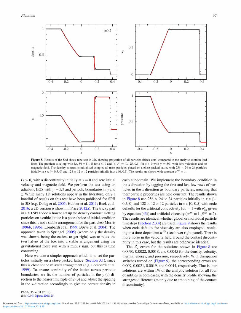
Phantom 37

Figure 8. Results of the Sod shock tube test in 3D, showing projection of all particles (black dots) compared to the analytic solution (redline). The problem is set up with [ρ, P] = [1, 1] for x � 0 and [ρ, P] = [0.125, 0.1] for x > 0 with γ = 5/3, with zero velocities and nomagnetic field. The density contrast is initialised using equal mass particles placed on a close packed lattice with 256 × 24 × 24 particlesinitially in x ∈ [− 0.5, 0] and 128 × 12 × 12 particles initially in x ∈ [0, 0.5]. The results are shown with constant αAV = 1.

(x > 0) with a discontinuity initially at x = 0 and zero initialvelocity and magnetic field. We perform the test using anadiabatic EOS with γ = 5/3 and periodic boundaries in y andz. While many 1D solutions appear in the literature, only ahandful of results on this test have been published for SPHin 3D (e.g. Dolag et al. 2005; Hubber et al. 2011; Beck et al.2016; a 2D version is shown in Price 2012a). The tricky partin a 3D SPH code is how to set up the density contrast. Settingparticles on a cubic lattice is a poor choice of initial conditionsince this is not a stable arrangement for the particles (Morris1996b, 1996a; Lombardi et al. 1999; Børve et al. 2004). Theapproach taken in Springel (2005) (where only the densitywas shown, being the easiest to get right) was to relax thetwo halves of the box into a stable arrangement using thegravitational force run with a minus sign, but this is timeconsuming.

Here we take a simpler approach which is to set the par-ticles initially on a close-packed lattice (Section 3.1), sincethis is close to the relaxed arrangement (e.g. Lombardi et al.1999). To ensure continuity of the lattice across periodicboundaries, we fix the number of particles in the y (z) di-rection to the nearest multiple of 2 (3) and adjust the spacingin the x-direction accordingly to give the correct density in

each subdomain. We implement the boundary condition inthe x-direction by tagging the first and last few rows of par-ticles in the x direction as boundary particles, meaning thattheir particle properties are held constant. The results shownin Figure 8 use 256 × 24 × 24 particles initially in x ∈ [−0.5, 0] and 128 × 12 × 12 particles in x ∈ [0, 0.5] with codedefaults for the artificial conductivity [αu = 1 with vu

sig givenby equation (43)] and artificial viscosity (αAV = 1, βAV = 2).The results are identical whether global or individual particletimesteps (Section 2.3.4) are used. Figure 9 shows the resultswhen code defaults for viscosity are also employed, result-ing in a time-dependent αAV (see lower right panel). There ismore noise in the velocity field around the contact disconti-nuity in this case, but the results are otherwise identical.

The L2 errors for the solutions shown in Figure 8 are0.0090, 0.0022, 0.0018, and 0.0045 for the density, velocity,thermal energy, and pressure, respectively. With dissipationswitches turned on (Figure 9), the corresponding errors are0.009, 0.0021, 0.0019, and 0.0044, respectively. That is, oursolutions are within 1% of the analytic solution for all fourquantities in both cases, with the density profile showing thestrongest difference (mainly due to smoothing of the contactdiscontinuity).

PASA, 35, e031 (2018)doi:10.1017/pasa.2018.25






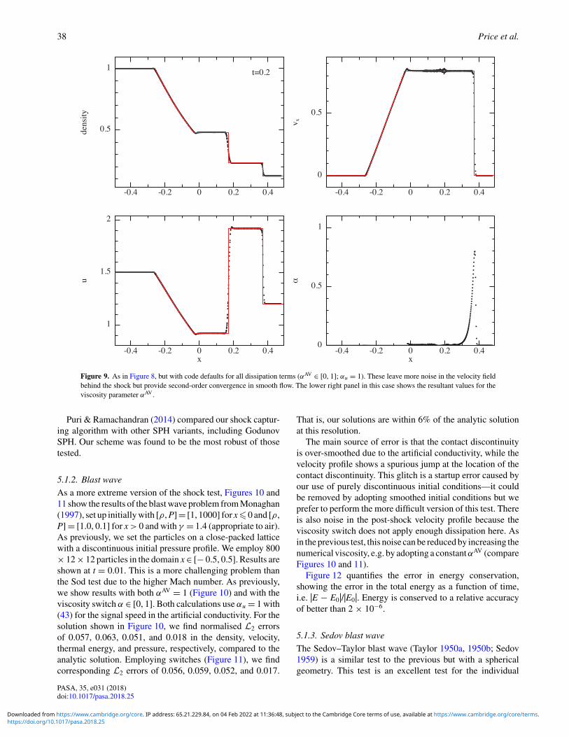
38 Price et al.

Figure 9. As in Figure 8, but with code defaults for all dissipation terms (αAV ∈ [0, 1]; αu = 1). These leave more noise in the velocity fieldbehind the shock but provide second-order convergence in smooth flow. The lower right panel in this case shows the resultant values for theviscosity parameter αAV.

Puri & Ramachandran (2014) compared our shock captur-ing algorithm with other SPH variants, including GodunovSPH. Our scheme was found to be the most robust of thosetested.

5.1.2. Blast wave

As a more extreme version of the shock test, Figures 10 and11 show the results of the blast wave problem from Monaghan(1997), set up initially with [ρ, P] = [1, 1000] for x�0 and [ρ,P] = [1.0, 0.1] for x > 0 and with γ = 1.4 (appropriate to air).As previously, we set the particles on a close-packed latticewith a discontinuous initial pressure profile. We employ 800× 12 × 12 particles in the domain x ∈ [− 0.5, 0.5]. Results areshown at t = 0.01. This is a more challenging problem thanthe Sod test due to the higher Mach number. As previously,we show results with both αAV = 1 (Figure 10) and with theviscosity switch α ∈ [0, 1]. Both calculations use αu = 1 with(43) for the signal speed in the artificial conductivity. For thesolution shown in Figure 10, we find normalised L2 errorsof 0.057, 0.063, 0.051, and 0.018 in the density, velocity,thermal energy, and pressure, respectively, compared to theanalytic solution. Employing switches (Figure 11), we findcorresponding L2 errors of 0.056, 0.059, 0.052, and 0.017.

That is, our solutions are within 6% of the analytic solutionat this resolution.

The main source of error is that the contact discontinuityis over-smoothed due to the artificial conductivity, while thevelocity profile shows a spurious jump at the location of thecontact discontinuity. This glitch is a startup error caused byour use of purely discontinuous initial conditions—it couldbe removed by adopting smoothed initial conditions but weprefer to perform the more difficult version of this test. Thereis also noise in the post-shock velocity profile because theviscosity switch does not apply enough dissipation here. Asin the previous test, this noise can be reduced by increasing thenumerical viscosity, e.g. by adopting a constant αAV (compareFigures 10 and 11).

Figure 12 quantifies the error in energy conservation,showing the error in the total energy as a function of time,i.e. |E − E0|/|E0|. Energy is conserved to a relative accuracyof better than 2 × 10−6.

5.1.3. Sedov blast wave

The Sedov–Taylor blast wave (Taylor 1950a, 1950b; Sedov1959) is a similar test to the previous but with a sphericalgeometry. This test is an excellent test for the individual

PASA, 35, e031 (2018)doi:10.1017/pasa.2018.25






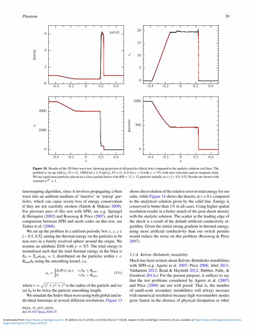
Phantom 39

Figure 10. Results of the 3D blast wave test, showing projection of all particles (black dots) compared to the analytic solution (red line). Theproblem is set up with [ρ, P] = [1, 1000] for x � 0 and [ρ, P] = [1, 0.1] for x > 0 with γ = 7/5, with zero velocities and no magnetic field.We use equal mass particles placed on a close packed lattice with 800 × 12 × 12 particles initially in x ∈ [− 0.5, 0.5]. Results are shown withconstant αAV = 1.

timestepping algorithm, since it involves propagating a blastwave into an ambient medium of ‘inactive’ or ‘asleep’ par-ticles, which can cause severe loss of energy conservationif they are not carefully awoken (Saitoh & Makino 2009).For previous uses of this test with SPH, see e.g. Springel& Hernquist (2002) and Rosswog & Price (2007), and for acomparison between SPH and mesh codes on this test, seeTasker et al. (2008).

We set up the problem in a uniform periodic box x, y, z ∈[− 0.5, 0.5], setting the thermal energy on the particles to benon-zero in a barely resolved sphere around the origin. Weassume an adiabatic EOS with γ = 5/3. The total energy isnormalised such that the total thermal energy in the blast isE0 = �amaua = 1, distributed on the particles within r <

Rkernh0 using the smoothing kernel, i.e.

ua ={

E0W (r, h0 ), r/h0 ≤ Rkern

0 r/h0 > Rkern,(311)

where r =√

x2 + y2 + z2 is the radius of the particle and weset h0 to be twice the particle smoothing length.

We simulate the Sedov blast wave using both global and in-dividual timesteps at several different resolutions. Figure 13

shows the evolution of the relative error in total energy for oursuite, while Figure 14 shows the density at t = 0.1 comparedto the analytical solution given by the solid line. Energy isconserved to better than 1% in all cases. Using higher spatialresolution results in a better match of the post-shock densitywith the analytic solution. The scatter at the leading edge ofthe shock is a result of the default artificial conductivity al-gorithm. Given the initial strong gradient in thermal energy,using more artificial conductivity than our switch permitswould reduce the noise on this problem (Rosswog & Price2007).

5.1.4. Kelvin–Helmholtz instability

Much has been written about Kelvin–Helmholtz instabilitieswith SPH (e.g. Agertz et al. 2007; Price 2008; Abel 2011;Valdarnini 2012; Read & Hayfield 2012; Hubber, Falle, &Goodwin 2013c). For the present purpose, it suffices to saythat the test problems considered by Agertz et al. (2007)and Price (2008) are not well posed. That is, the numberof small-scale secondary instabilities will always increasewith numerical resolution because high wavenumber modesgrow fastest in the absence of physical dissipation or other

PASA, 35, e031 (2018)doi:10.1017/pasa.2018.25






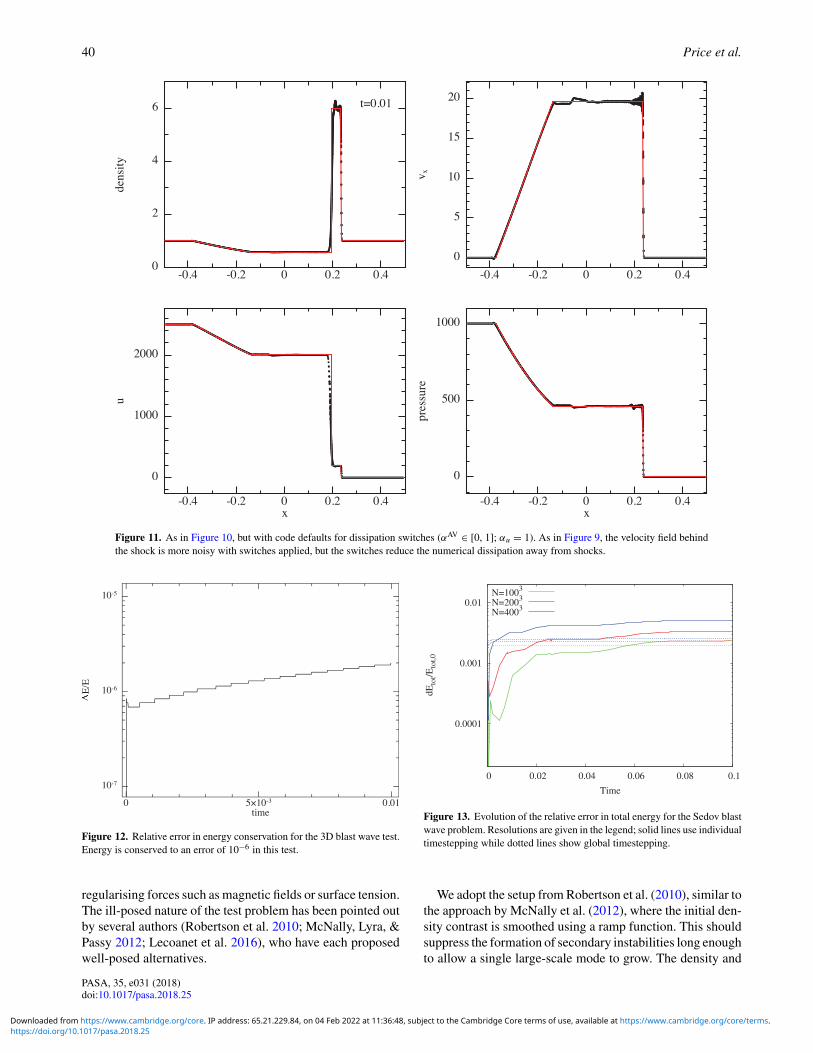
40 Price et al.

Figure 11. As in Figure 10, but with code defaults for dissipation switches (αAV ∈ [0, 1]; αu = 1). As in Figure 9, the velocity field behindthe shock is more noisy with switches applied, but the switches reduce the numerical dissipation away from shocks.

Figure 12. Relative error in energy conservation for the 3D blast wave test.Energy is conserved to an error of 10−6 in this test.

regularising forces such as magnetic fields or surface tension.The ill-posed nature of the test problem has been pointed outby several authors (Robertson et al. 2010; McNally, Lyra, &Passy 2012; Lecoanet et al. 2016), who have each proposedwell-posed alternatives.

0.0001

0.001

0.01

0 0.02 0.04 0.06 0.08 0.1

dEto

t/Eto

t,0

Time

N=1003

N=2003

N=4003

Figure 13. Evolution of the relative error in total energy for the Sedov blastwave problem. Resolutions are given in the legend; solid lines use individualtimestepping while dotted lines show global timestepping.

We adopt the setup from Robertson et al. (2010), similar tothe approach by McNally et al. (2012), where the initial den-sity contrast is smoothed using a ramp function. This shouldsuppress the formation of secondary instabilities long enoughto allow a single large-scale mode to grow. The density and

PASA, 35, e031 (2018)doi:10.1017/pasa.2018.25






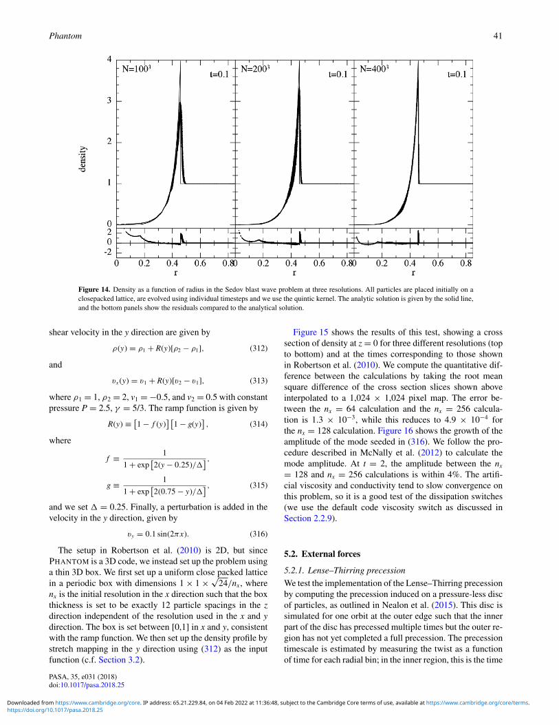
Phantom 41

Figure 14. Density as a function of radius in the Sedov blast wave problem at three resolutions. All particles are placed initially on aclosepacked lattice, are evolved using individual timesteps and we use the quintic kernel. The analytic solution is given by the solid line,and the bottom panels show the residuals compared to the analytical solution.

shear velocity in the y direction are given by

ρ(y) = ρ1 + R(y)[ρ2 − ρ1], (312)

and

vx (y) = v1 + R(y)[v2 − v1], (313)

where ρ1 = 1, ρ2 = 2, v1 = −0.5, and v2 = 0.5 with constantpressure P = 2.5, γ = 5/3. The ramp function is given by

R(y) ≡ [1 − f (y)

] [1 − g(y)

], (314)

where

f ≡ 1

1 + exp[2(y − 0.25)/�

] ,g ≡ 1

1 + exp[2(0.75 − y)/�

] , (315)

and we set � = 0.25. Finally, a perturbation is added in thevelocity in the y direction, given by

vy = 0.1 sin(2πx). (316)

The setup in Robertson et al. (2010) is 2D, but sincePHANTOM is a 3D code, we instead set up the problem usinga thin 3D box. We first set up a uniform close packed latticein a periodic box with dimensions 1 × 1 × √

24/nx, wherenx is the initial resolution in the x direction such that the boxthickness is set to be exactly 12 particle spacings in the zdirection independent of the resolution used in the x and ydirection. The box is set between [0,1] in x and y, consistentwith the ramp function. We then set up the density profile bystretch mapping in the y direction using (312) as the inputfunction (c.f. Section 3.2).

Figure 15 shows the results of this test, showing a crosssection of density at z = 0 for three different resolutions (topto bottom) and at the times corresponding to those shownin Robertson et al. (2010). We compute the quantitative dif-ference between the calculations by taking the root meansquare difference of the cross section slices shown aboveinterpolated to a 1,024 × 1,024 pixel map. The error be-tween the nx = 64 calculation and the nx = 256 calcula-tion is 1.3 × 10−3, while this reduces to 4.9 × 10−4 forthe nx = 128 calculation. Figure 16 shows the growth of theamplitude of the mode seeded in (316). We follow the pro-cedure described in McNally et al. (2012) to calculate themode amplitude. At t = 2, the amplitude between the nx

= 128 and nx = 256 calculations is within 4%. The artifi-cial viscosity and conductivity tend to slow convergence onthis problem, so it is a good test of the dissipation switches(we use the default code viscosity switch as discussed inSection 2.2.9).

5.2. External forces

5.2.1. Lense–Thirring precession

We test the implementation of the Lense–Thirring precessionby computing the precession induced on a pressure-less discof particles, as outlined in Nealon et al. (2015). This disc issimulated for one orbit at the outer edge such that the innerpart of the disc has precessed multiple times but the outer re-gion has not yet completed a full precession. The precessiontimescale is estimated by measuring the twist as a functionof time for each radial bin; in the inner region, this is the time

PASA, 35, e031 (2018)doi:10.1017/pasa.2018.25






42 Price et al.

Figure 15. Results of the well-posed Kelvin–Helmholtz instability test from Robertson et al. (2010), shown at a resolution of (from top to bottom) 64 × 74× 12, 128 × 148 × 12 and 256 × 296 × 12 equal mass SPH particles. We use stretch mapping (Section 3.2) to achieve the initial density profile, consistingof a 2:1 density jump with a smoothed transition.

0

0.1

0.2

0.3

0.4

0.5

0 0.5 1 1.5 2

Mod

eam

plitu

de

t

nx = 64nx = 128nx = 256

Figure 16. Growth of the amplitude of the seeded mode for the Kevin–Helmholtz instability test. The amplitude at t = 2 between the nx = 128 andnx = 256 calculations is within 4%.

taken for the twist to go from a minimum (zero twist) to amaximum (fully twisted) and in the outer region the gra-dient of the twist against time is used to calculate theequivalent time. Figure 17 shows the precession timescale

Figure 17. Lense–Thirring precession test from a disc inclined by 30°. Here,the precession timescale is measured from the cumulative twist in the discand the exact solution, tp = R3/2a is represented by the red line.

measured from the simulation as a function of the radiuscompared to the analytically derived precession timescale,with uncertainties derived from the calculation of thegradient.

PASA, 35, e031 (2018)doi:10.1017/pasa.2018.25






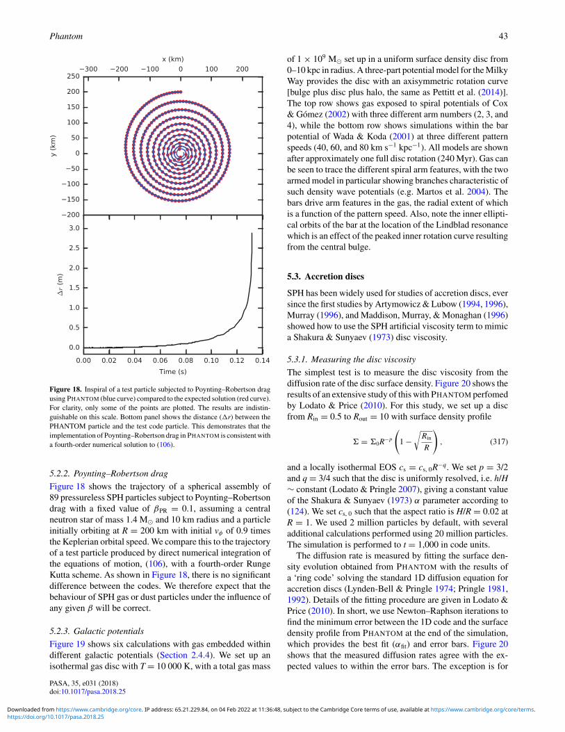
Phantom 43

Figure 18. Inspiral of a test particle subjected to Poynting–Robertson dragusing PHANTOM (blue curve) compared to the expected solution (red curve).For clarity, only some of the points are plotted. The results are indistin-guishable on this scale. Bottom panel shows the distance (�r) between thePHANTOM particle and the test code particle. This demonstrates that theimplementation of Poynting–Robertson drag in PHANTOM is consistent witha fourth-order numerical solution to (106).

5.2.2. Poynting–Robertson drag

Figure 18 shows the trajectory of a spherical assembly of89 pressureless SPH particles subject to Poynting–Robertsondrag with a fixed value of βPR = 0.1, assuming a centralneutron star of mass 1.4 M� and 10 km radius and a particleinitially orbiting at R = 200 km with initial vφ of 0.9 timesthe Keplerian orbital speed. We compare this to the trajectoryof a test particle produced by direct numerical integration ofthe equations of motion, (106), with a fourth-order RungeKutta scheme. As shown in Figure 18, there is no significantdifference between the codes. We therefore expect that thebehaviour of SPH gas or dust particles under the influence ofany given β will be correct.

5.2.3. Galactic potentials

Figure 19 shows six calculations with gas embedded withindifferent galactic potentials (Section 2.4.4). We set up anisothermal gas disc with T = 10 000 K, with a total gas mass

of 1 × 109 M� set up in a uniform surface density disc from0–10 kpc in radius. A three-part potential model for the MilkyWay provides the disc with an axisymmetric rotation curve[bulge plus disc plus halo, the same as Pettitt et al. (2014)].The top row shows gas exposed to spiral potentials of Cox& Gómez (2002) with three different arm numbers (2, 3, and4), while the bottom row shows simulations within the barpotential of Wada & Koda (2001) at three different patternspeeds (40, 60, and 80 km s−1 kpc−1). All models are shownafter approximately one full disc rotation (240 Myr). Gas canbe seen to trace the different spiral arm features, with the twoarmed model in particular showing branches characteristic ofsuch density wave potentials (e.g. Martos et al. 2004). Thebars drive arm features in the gas, the radial extent of whichis a function of the pattern speed. Also, note the inner ellipti-cal orbits of the bar at the location of the Lindblad resonancewhich is an effect of the peaked inner rotation curve resultingfrom the central bulge.

5.3. Accretion discs

SPH has been widely used for studies of accretion discs, eversince the first studies by Artymowicz & Lubow (1994, 1996),Murray (1996), and Maddison, Murray, & Monaghan (1996)showed how to use the SPH artificial viscosity term to mimica Shakura & Sunyaev (1973) disc viscosity.

5.3.1. Measuring the disc viscosity

The simplest test is to measure the disc viscosity from thediffusion rate of the disc surface density. Figure 20 shows theresults of an extensive study of this with PHANTOM perfomedby Lodato & Price (2010). For this study, we set up a discfrom Rin = 0.5 to Rout = 10 with surface density profile

� = �0R−p

(1 −

√Rin

R

), (317)

and a locally isothermal EOS cs = cs, 0R−q. We set p = 3/2and q = 3/4 such that the disc is uniformly resolved, i.e. h/H∼ constant (Lodato & Pringle 2007), giving a constant valueof the Shakura & Sunyaev (1973) α parameter according to(124). We set cs, 0 such that the aspect ratio is H/R = 0.02 atR = 1. We used 2 million particles by default, with severaladditional calculations performed using 20 million particles.The simulation is performed to t = 1,000 in code units.

The diffusion rate is measured by fitting the surface den-sity evolution obtained from PHANTOM with the results ofa ‘ring code’ solving the standard 1D diffusion equation foraccretion discs (Lynden-Bell & Pringle 1974; Pringle 1981,1992). Details of the fitting procedure are given in Lodato &Price (2010). In short, we use Newton–Raphson iterations tofind the minimum error between the 1D code and the surfacedensity profile from PHANTOM at the end of the simulation,which provides the best fit (αfit) and error bars. Figure 20shows that the measured diffusion rates agree with the ex-pected values to within the error bars. The exception is for

PASA, 35, e031 (2018)doi:10.1017/pasa.2018.25






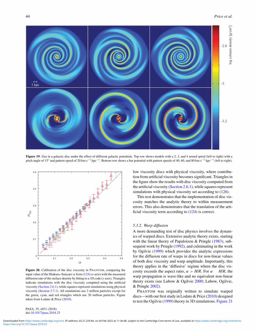
44 Price et al.

1 kpc

-3.2

-3

-2.8

log

colu

mn

dens

ity

[g/c

m2 ]

Figure 19. Gas in a galactic disc under the effect of different galactic potentials. Top row shows models with a 2, 3, and 4 armed spiral (left to right) with apitch angle of 15° and pattern speed of 20 km s−1 kpc−1. Bottom row shows a bar potential with pattern speeds of 40, 60, and 80 km s−1 kpc−1 (left to right).

0 0.1 0.2 0.3 0.4 0.50

0.1

0.2

0.3

0.4

0.5

Figure 20. Calibration of the disc viscosity in PHANTOM, comparing theinput value of the Shakura–Sunyaev α from (124) (x-axis) with the measureddiffusion rate of the surface density by fitting to a 1D code (y-axis). Trianglesindicate simulations with the disc viscosity computed using the artificialviscosity (Section 2.6.1), while squares represent simulations using physicalviscosity (Section 2.7.1). All simulations use 2 million particles except forthe green, cyan, and red triangles which use 20 million particles. Figuretaken from Lodato & Price (2010).

low viscosity discs with physical viscosity, where contribu-tion from artificial viscosity becomes significant. Triangles inthe figure show the results with disc viscosity computed fromthe artificial viscosity (Section 2.6.1), while squares representsimulations with physical viscosity set according to (126).

This test demonstrates that the implementation of disc vis-cosity matches the analytic theory to within measurementerrors. This also demonstrates that the translation of the arti-ficial viscosity term according to (124) is correct.

5.3.2. Warp diffusion

A more demanding test of disc physics involves the dynam-ics of warped discs. Extensive analytic theory exists, startingwith the linear theory of Papaloizou & Pringle (1983), sub-sequent work by Pringle (1992), and culminating in the workby Ogilvie (1999) which provides the analytic expressionsfor the diffusion rate of warps in discs for non-linear valuesof both disc viscosity and warp amplitude. Importantly, thistheory applies in the ‘diffusive’ regime where the disc vis-cosity exceeds the aspect ratio, α > H/R. For α � H/R, thewarp propagation is wave-like and no equivalent non-lineartheory exists (see Lubow & Ogilvie 2000; Lubow, Ogilvie,& Pringle 2002).

PHANTOM was originally written to simulate warpeddiscs—with our first study in Lodato & Price (2010) designedto test the Ogilvie (1999) theory in 3D simulations. Figure 21

PASA, 35, e031 (2018)doi:10.1017/pasa.2018.25






Phantom 45

0 0.1 0.2 0.3 0.4 0.50

2

4

6

8

10

Figure 21. Warp diffusion rate as a function of disc viscosity, showing thePHANTOM results compared to the non-linear theory of Ogilvie (1999)(dashed line). The linear prediction, α2 = 1/(2α), is shown by the solidline, highlighting the agreement of PHANTOM with the non-linear theory.Colouring of points is as in Figure 20. Figure taken from Lodato & Price(2010).

shows the results of this study, showing the measured warpdiffusion rate as a function of disc viscosity. The setup of thesimulations is as in the previous test but with a small warpadded to the disc, as outlined in Section 3.3 of Lodato & Price(2010). Details of the fitting procedure used to measure thewarp diffusion rate are also given in Section 4.2 of that paper.The dashed line shows the non-linear prediction of Ogilvie(1999), namely

α2 = 1

2α

4(1 + 7α2)

4 + α2. (318)

Significantly, the PHANTOM results show a measurable dif-ference between the predictions of the non-linear theory andthe prediction from linear theory (Papaloizou & Pringle 1983)of α2 = 1/(2α), shown by the solid black line.

In addition to the results shown in Figure 21, PHANTOM

also showed a close match to both the predicted self-inducedprecession of the warp and to the evolution of non-linearwarps (see Figures 13 and 14 in Lodato & Price 2010, respec-tively). From the success of this initial study, we have usedPHANTOM to study many aspects of disc warping, either withisolated warps or breaks (Lodato & Price 2010; Nixon et al.2012a), warps induced by spinning black holes (Nixon et al.2012b; Nealon et al. 2015, 2016), and warps in circumbinary(Nixon et al. 2013; Facchini et al. 2013) or circumprimary(Dogan et al. 2015; Martin et al. 2014a, 2014b) discs. In par-ticular, PHANTOM was used to discover the phenomenon of‘disc tearing’ where sections of the disc are ‘torn’ from thedisc plane and precess effectively independently (Nixon et al.2012b, 2013; Nealon et al. 2015).

Figure 22. Planet–disc interaction in 3D, showing the ‘viscous Jupiter’ cal-culation comparable to the 2D results shown with various grid and SPHcodes in Figure 10 of de Val-Borro et al. (2006). The dotted lines shows theestimated position of the planetary shocks from Ogilvie & Lubow (2002).The offset between this solution and the numerical shock position is dueto the approximate nature of the analytic solution (see de Val-Borro et al.2006).

5.3.3. Disc–planet interaction

Although there is no ‘exact’ solution for planet–disc inter-action, an extensive code comparison was performed by deVal-Borro et al. (2006). Figure 22 shows the column densityof a 3D PHANTOM calculation, plotted in r–φ with the densityintegrated through the z direction, comparable to the ‘viscousJupiter’ setup in de Val-Borro et al. (2006).

Two caveats apply when comparing our results with thosein Figure 10 of de Val-Borro et al. (2006). The first is thatthe original comparison project was performed in 2D andmainly with grid-based codes with specific ‘wave damping’boundary conditions prescribed. We chose simply to ignorethe prescribed boundary conditions and two dimensionalityand instead modelled the disc in 3D with a central accretionboundary at r = 0.25 with a free outer boundary, with theinitial disc set up from r = 0.4 to r = 2.5. We used 106

SPH particles. Second, the planetary orbit was prescribedon a fixed circular orbit with no accretion onto either theplanet or the star. Although we usually use sink particles inPHANTOM to model planet–disc interaction (e.g. Dipierroet al. 2015), for this test we thus employed the fixed binarypotential (Section 2.4.2) to enable a direct comparison. Wethus used M = 10−3 in the binary potential, corresponding tothe ‘Jupiter’ simulation in de Val-Borro et al. (2006) with theplanet on a fixed circular orbit at r = 1.

As per the original comparison project, we implementedPlummer softening of the gravitational force from the planet

φplanet = − −mplanet√r2 + ε2

, (319)

PASA, 35, e031 (2018)doi:10.1017/pasa.2018.25






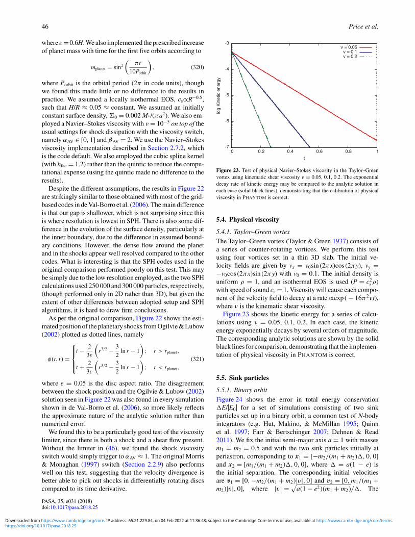
46 Price et al.

where ε =0.6H. We also implemented the prescribed increaseof planet mass with time for the first five orbits according to

mplanet = sin2

(πt

10Porbit

), (320)

where Porbit is the orbital period (2π in code units), thoughwe found this made little or no difference to the results inpractice. We assumed a locally isothermal EOS, cs∝R−0.5,such that H/R ≈ 0.05 ≈ constant. We assumed an initiallyconstant surface density, �0 = 0.002 M∗ /(πa2). We also em-ployed a Navier–Stokes viscosity with ν = 10−5 on top of theusual settings for shock dissipation with the viscosity switch,namely αAV ∈ [0, 1] and βAV = 2. We use the Navier–Stokesviscosity implementation described in Section 2.7.2, whichis the code default. We also employed the cubic spline kernel(with hfac = 1.2) rather than the quintic to reduce the compu-tational expense (using the quintic made no difference to theresults).

Despite the different assumptions, the results in Figure 22are strikingly similar to those obtained with most of the grid-based codes in de Val-Borro et al. (2006). The main differenceis that our gap is shallower, which is not surprising since thisis where resolution is lowest in SPH. There is also some dif-ference in the evolution of the surface density, particularly atthe inner boundary, due to the difference in assumed bound-ary conditions. However, the dense flow around the planetand in the shocks appear well resolved compared to the othercodes. What is interesting is that the SPH codes used in theoriginal comparison performed poorly on this test. This maybe simply due to the low resolution employed, as the two SPHcalculations used 250 000 and 300 000 particles, respectively,(though performed only in 2D rather than 3D), but given theextent of other differences between adopted setup and SPHalgorithms, it is hard to draw firm conclusions.

As per the original comparison, Figure 22 shows the esti-mated position of the planetary shocks from Ogilvie & Lubow(2002) plotted as dotted lines, namely

φ(r, t ) =

⎧⎪⎪⎨⎪⎪⎩

t − 2

3ε

(r3/2 − 3

2ln r − 1

); r > rplanet,

t + 2

3ε

(r3/2 − 3

2ln r − 1

); r < rplanet,

(321)

where ε = 0.05 is the disc aspect ratio. The disagreementbetween the shock position and the Ogilvie & Lubow (2002)solution seen in Figure 22 was also found in every simulationshown in de Val-Borro et al. (2006), so more likely reflectsthe approximate nature of the analytic solution rather thannumerical error.

We found this to be a particularly good test of the viscositylimiter, since there is both a shock and a shear flow present.Without the limiter in (46), we found the shock viscosityswitch would simply trigger to αAV ≈ 1. The original Morris& Monaghan (1997) switch (Section 2.2.9) also performswell on this test, suggesting that the velocity divergence isbetter able to pick out shocks in differentially rotating discscompared to its time derivative.

Figure 23. Test of physical Navier–Stokes viscosity in the Taylor–Greenvortex using kinematic shear viscosity ν = 0.05, 0.1, 0.2. The exponentialdecay rate of kinetic energy may be compared to the analytic solution ineach case (solid black lines), demonstrating that the calibration of physicalviscosity in PHANTOM is correct.

5.4. Physical viscosity

5.4.1. Taylor–Green vortex

The Taylor–Green vortex (Taylor & Green 1937) consists ofa series of counter-rotating vortices. We perform this testusing four vortices set in a thin 3D slab. The initial ve-locity fields are given by vx = v0sin (2πx)cos (2πy), vy =−v0cos (2πx)sin (2πy) with v0 = 0.1. The initial density isuniform ρ = 1, and an isothermal EOS is used (P = c2

s ρ)with speed of sound cs = 1. Viscosity will cause each compo-nent of the velocity field to decay at a rate ∝exp ( − 16π2νt),where ν is the kinematic shear viscosity.

Figure 23 shows the kinetic energy for a series of calcu-lations using ν = 0.05, 0.1, 0.2. In each case, the kineticenergy exponentially decays by several orders of magnitude.The corresponding analytic solutions are shown by the solidblack lines for comparison, demonstrating that the implemen-tation of physical viscosity in PHANTOM is correct.

5.5. Sink particles

5.5.1. Binary orbit

Figure 24 shows the error in total energy conservation�E/|E0| for a set of simulations consisting of two sinkparticles set up in a binary orbit, a common test of N-bodyintegrators (e.g. Hut, Makino, & McMillan 1995; Quinnet al. 1997; Farr & Bertschinger 2007; Dehnen & Read2011). We fix the initial semi-major axis a = 1 with massesm1 = m2 = 0.5 and with the two sink particles initially atperiastron, corresponding to x1 = [−m2/(m1 + m2)�, 0, 0]and x2 = [m1/(m1 + m2)�, 0, 0], where � = a(1 − e) isthe initial separation. The corresponding initial velocitiesare v1 = [0,−m2/(m1 + m2)|v|, 0] and v2 = [0, m1/(m1 +m2)|v|, 0], where |v| =

√a(1 − e2)(m1 + m2)/�. The

PASA, 35, e031 (2018)doi:10.1017/pasa.2018.25






Phantom 47

Figure 24. Errors in energy conservation in a sink particle binary integrationwith code default parameters for the timestep control, showing the energydrift caused by the adaptive timestepping. Angular momentum is conservedto machine precision.

orbital period is thus P =√

4π2a3/(G(m1 + m2)) = 2π incode units for our chosen parameters. Importantly, we usean adaptive timestep which is not time symmetric so thereremains some drift in the energy error which is absent ifthe timestep is constant (see e.g. Hut et al. 1995; Quinnet al. 1997 and Dehnen & Read 2011 for discussion of thisissue).

Figure 24 shows the error in total energy as a functionof time for the first 1,000 orbits for calculations with initialeccentricities of e = 0.0 (a circular orbit), 0.3, 0.5, 0.7, and0.9. Energy conservation is worse for more eccentric orbits,as expected, with �E/|E0| ∼ 6% after 1,000 orbits for ourmost extreme case (e = 0.9). The energy error can be reducedarbitrarily by decreasing the timestep, so this is mainly a testof the default settings for the sink particle timestep control.For this problem, the timestep is controlled entirely by (76),where by default we use η� = 0.05, giving 474 steps per orbitfor e = 0.9. For simulations with more eccentric orbits, werecommend decreasing Cforce from the default setting of 0.25to obtain more accurate orbital dynamics.

In addition to calibrating the timestep constraint, Figure 24also validates the sink particle substepping via the RESPAalgorithm (Section 2.3.3) since for this problem the ‘gas’timestep is set only by the desired interval between out-put files (to ensure sufficient output for the figure wechoose �tmax = 1, but we also confirmed that this choiceis unimportant for the resultant energy conservation). Thismeans that increasing the accuracy of sink particle inter-actions adds little or no cost to calculations involving gasparticles.

The corresponding plot for angular momentum conserva-tion (not shown) merely demonstrates that angular momen-tum is conserved to machine precision (�L/|L| ∼ 10−15),as expected. Importantly, angular momentum remains con-served to machine precision even with adaptive timestepping.

Figure 25. Orbit of a sink particle in the restricted three-body problem fromChin & Chen (2005) using default code parameters. This tests both the timeintegrator for sink particles and the interaction with a time-dependent binarypotential (Section 2.4.2). The trajectory of the sink is plotted every timestepfor three periods (t = 27π ).

5.5.2. Restricted three-body problem

Chin & Chen (2005) proposed a more demanding test ofN-body integrators, consisting of a test particle orbitingin the potential of a binary on a fixed circular orbit. Weset up this problem with a single sink particle with x =[0, 0.0580752367, 0] and v = [0.489765446, 0, 0], using thetime-dependent binary potential as described in Section 2.4.2with M = 0.5. This is therefore a good test of the interactionbetween a sink particle and external potentials in the code, aswell as the sink particle timestepping algorithm. For conve-nience, we set the sink mass m = 1 and accretion radius racc

= 0.1, although both are irrelevant to the problem.Figure 25 shows the resulting orbit using the default code

parameters, where we plot the trajectory of the sink parti-cle up to t = 27π , as in Figures 1 and 2 of Chin & Chen(2005). Considering that we use only a second-order integra-tor, the orbital trajectory is remarkably accurate, showing nochaotic behaviour and only a slight precession consistent orbetter than the results with some of the fourth-order schemesshown in their paper (albeit computed with a larger timestep).We are thus satisfied that our time integration scheme and theassociated timestep settings can capture complex orbital dy-namics with sufficient accuracy.

5.6. Magnetohydrodynamics

5.6.1. 3D circularly polarised Alfvén wave

Tóth (2000) introduced the circularly polarised Alfvén wavetest, an exact non-linear solution to the MHD equations whichcan therefore be performed using a wave of arbitrarily large

PASA, 35, e031 (2018)doi:10.1017/pasa.2018.25






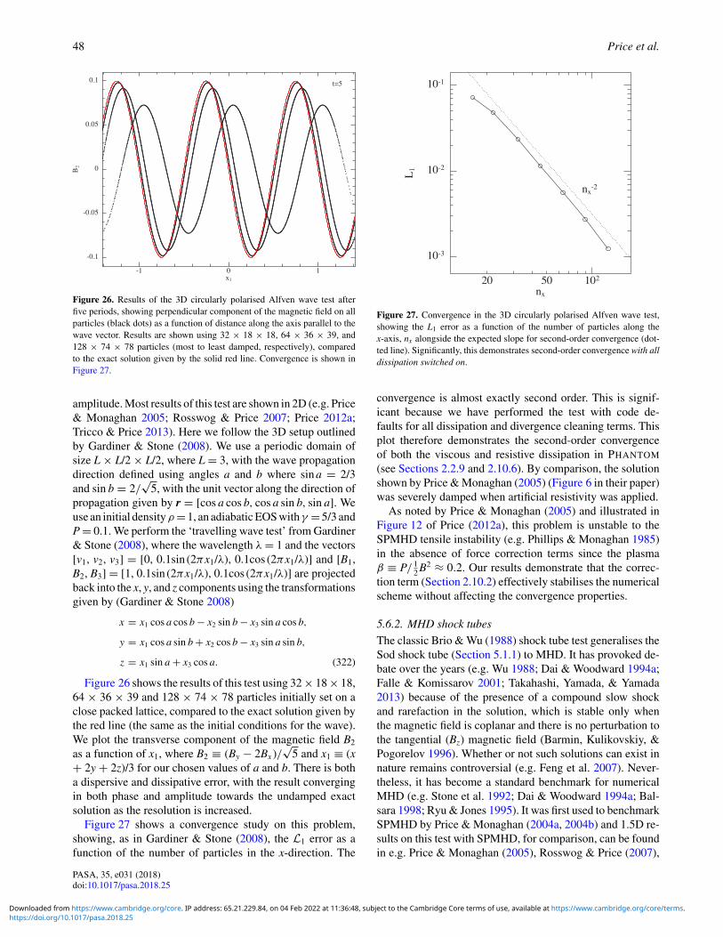
48 Price et al.

Figure 26. Results of the 3D circularly polarised Alfven wave test afterfive periods, showing perpendicular component of the magnetic field on allparticles (black dots) as a function of distance along the axis parallel to thewave vector. Results are shown using 32 × 18 × 18, 64 × 36 × 39, and128 × 74 × 78 particles (most to least damped, respectively), comparedto the exact solution given by the solid red line. Convergence is shown inFigure 27.

amplitude. Most results of this test are shown in 2D (e.g. Price& Monaghan 2005; Rosswog & Price 2007; Price 2012a;Tricco & Price 2013). Here we follow the 3D setup outlinedby Gardiner & Stone (2008). We use a periodic domain ofsize L × L/2 × L/2, where L = 3, with the wave propagationdirection defined using angles a and b where sin a = 2/3and sin b = 2/

√5, with the unit vector along the direction of

propagation given by r = [cos a cos b, cos a sin b, sin a]. Weuse an initial densityρ =1, an adiabatic EOS withγ =5/3 andP = 0.1. We perform the ‘travelling wave test’ from Gardiner& Stone (2008), where the wavelength λ = 1 and the vectors[v1, v2, v3] = [0, 0.1sin (2πx1/λ), 0.1cos (2πx1/λ)] and [B1,B2, B3] = [1, 0.1sin (2πx1/λ), 0.1cos (2πx1/λ)] are projectedback into the x, y, and z components using the transformationsgiven by (Gardiner & Stone 2008)

x = x1 cos a cos b − x2 sin b − x3 sin a cos b,

y = x1 cos a sin b + x2 cos b − x3 sin a sin b,

z = x1 sin a + x3 cos a. (322)

Figure 26 shows the results of this test using 32 × 18 × 18,64 × 36 × 39 and 128 × 74 × 78 particles initially set on aclose packed lattice, compared to the exact solution given bythe red line (the same as the initial conditions for the wave).We plot the transverse component of the magnetic field B2

as a function of x1, where B2 ≡ (By − 2Bx )/√

5 and x1 ≡ (x+ 2y + 2z)/3 for our chosen values of a and b. There is botha dispersive and dissipative error, with the result convergingin both phase and amplitude towards the undamped exactsolution as the resolution is increased.

Figure 27 shows a convergence study on this problem,showing, as in Gardiner & Stone (2008), the L1 error as afunction of the number of particles in the x-direction. The

Figure 27. Convergence in the 3D circularly polarised Alfven wave test,showing the L1 error as a function of the number of particles along thex-axis, nx alongside the expected slope for second-order convergence (dot-ted line). Significantly, this demonstrates second-order convergence with alldissipation switched on.

convergence is almost exactly second order. This is signif-icant because we have performed the test with code de-faults for all dissipation and divergence cleaning terms. Thisplot therefore demonstrates the second-order convergenceof both the viscous and resistive dissipation in PHANTOM

(see Sections 2.2.9 and 2.10.6). By comparison, the solutionshown by Price & Monaghan (2005) (Figure 6 in their paper)was severely damped when artificial resistivity was applied.

As noted by Price & Monaghan (2005) and illustrated inFigure 12 of Price (2012a), this problem is unstable to theSPMHD tensile instability (e.g. Phillips & Monaghan 1985)in the absence of force correction terms since the plasmaβ ≡ P/ 1

2 B2 ≈ 0.2. Our results demonstrate that the correc-tion term (Section 2.10.2) effectively stabilises the numericalscheme without affecting the convergence properties.

5.6.2. MHD shock tubes

The classic Brio & Wu (1988) shock tube test generalises theSod shock tube (Section 5.1.1) to MHD. It has provoked de-bate over the years (e.g. Wu 1988; Dai & Woodward 1994a;Falle & Komissarov 2001; Takahashi, Yamada, & Yamada2013) because of the presence of a compound slow shockand rarefaction in the solution, which is stable only whenthe magnetic field is coplanar and there is no perturbation tothe tangential (Bz) magnetic field (Barmin, Kulikovskiy, &Pogorelov 1996). Whether or not such solutions can exist innature remains controversial (e.g. Feng et al. 2007). Never-theless, it has become a standard benchmark for numericalMHD (e.g. Stone et al. 1992; Dai & Woodward 1994a; Bal-sara 1998; Ryu & Jones 1995). It was first used to benchmarkSPMHD by Price & Monaghan (2004a, 2004b) and 1.5D re-sults on this test with SPMHD, for comparison, can be foundin e.g. Price & Monaghan (2005), Rosswog & Price (2007),

PASA, 35, e031 (2018)doi:10.1017/pasa.2018.25






Phantom 49

Figure 28. Results of the Brio & Wu (1988) shock tube test in 3D, showing projection of all particles (black dots) compared to the referencesolution (red line). The problem is set up with [ρ, P, By, Bz] = [1, 1, 1, 0] for x � 0 and [ρ, P, By, Bz] = [0.125, 0.1, −1, 0] for x > 0 withzero initial velocities, Bx = 0.75 and γ = 2. The density contrast is initialised using equal mass particles placed on a close packed lattice with256 × 24 × 24 particles initially in x ∈ [− 0.5, 0] and 128 × 12 × 12 particles initially in x ∈ [0, 0.5].

Dolag & Stasyszyn (2009), Price (2010), and Vanaverbeke,Keppens, & Poedts (2014), with 2D versions shown in Price(2012a), Tricco & Price (2013), and Tricco et al. (2016a). Wehandle the boundary conditions by setting the first and last fewplanes of particles to be ‘boundary particles’ (Section A.2),meaning that the gas properties on these particles are fixed.

Figure 28 shows the results of the Brio & Wu (1988) prob-lem using PHANTOM, performed in 3D with 256 × 24 × 24particles initially in x ∈ [− 0.5, 0] and 128 × 12 × 12 parti-cles initially in x ∈ [0, 0.5] set on close packed lattices withpurely discontinuous initial conditions in the other variables(see caption). The projection of all particles onto the x-axis areshown as black dots, while the red lines shows a reference so-lution taken from Balsara (1998). Figure 28 shows the resultswhen a constant αAV = 1 is employed, while Figure 29 showsthe results with default code parameters, giving second-orderdissipation away from shocks. For constant αAV (Figure 28),we find the strongest deviation from the reference solution isin vx, withL1 = 0.015 andL2 = 0.065 at this resolution. Theremaining L2 errors are within 5% of the reference solution,while the L1 norms are all smaller than 1.5% per cent in theother variables. Similar errors are found with code defaults

(Figure 29), withL2 = 0.074 in vx andL1 norms smaller than1.6% in all variables. That is, our solutions are within 1.6%of the reference solution. Using the default Courant factorof 0.3, total energy is conserved to better than 0.5%, withmaximum |�E|/|E0| = 4.2 × 10−3 up to t = 0.1.

Figure 30 shows the result of the ‘seven-discontinuity’test from Ryu & Jones (1995). This test is particularlysensitive to over-dissipation by resistivity given the sharpjumps in the transverse magnetic and velocity fields. A ref-erence solution with intermediate states taken from the cor-responding table in Ryu & Jones (1995) is shown by thered lines for comparison. Here the boundary particles aremoved with a fixed velocity in the x-direction. The largestdeviation from the reference solution is in the vy compo-nent, mainly due to the over-dissipation of the small spikes,with L1 = 0.02 and L2 = 0.07 at this resolution. The re-maining L2 errors are within 3% of the reference solu-tion, while the L1 norms are smaller than 0.9% in all othervariables.

Finally, Figure 31 shows the results of shock tube 1a fromRyu & Jones (1995). This test is interesting because it hashistorically proven to be a difficult test for SPMHD codes in

PASA, 35, e031 (2018)doi:10.1017/pasa.2018.25






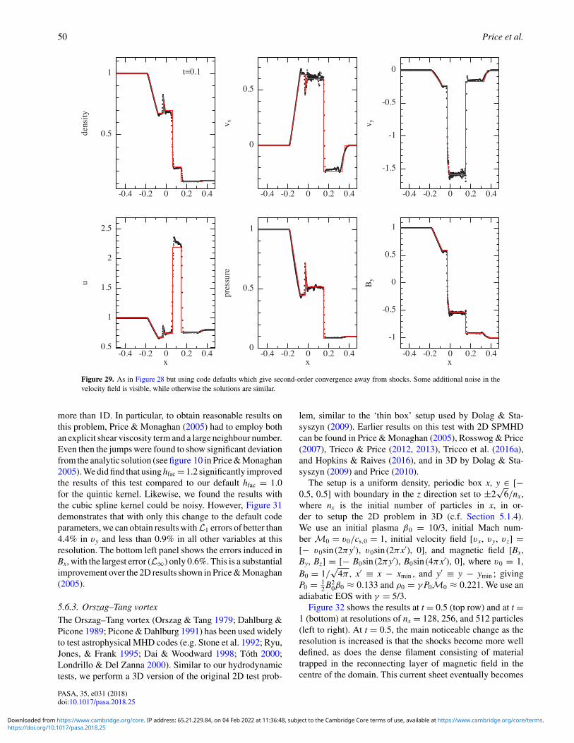
50 Price et al.

Figure 29. As in Figure 28 but using code defaults which give second-order convergence away from shocks. Some additional noise in thevelocity field is visible, while otherwise the solutions are similar.

more than 1D. In particular, to obtain reasonable results onthis problem, Price & Monaghan (2005) had to employ bothan explicit shear viscosity term and a large neighbour number.Even then the jumps were found to show significant deviationfrom the analytic solution (see figure 10 in Price & Monaghan2005). We did find that using hfac =1.2 significantly improvedthe results of this test compared to our default hfac = 1.0for the quintic kernel. Likewise, we found the results withthe cubic spline kernel could be noisy. However, Figure 31demonstrates that with only this change to the default codeparameters, we can obtain results withL1 errors of better than4.4% in vy and less than 0.9% in all other variables at thisresolution. The bottom left panel shows the errors induced inBx, with the largest error (L∞) only 0.6%. This is a substantialimprovement over the 2D results shown in Price & Monaghan(2005).

5.6.3. Orszag–Tang vortex

The Orszag–Tang vortex (Orszag & Tang 1979; Dahlburg &Picone 1989; Picone & Dahlburg 1991) has been used widelyto test astrophysical MHD codes (e.g. Stone et al. 1992; Ryu,Jones, & Frank 1995; Dai & Woodward 1998; Tóth 2000;Londrillo & Del Zanna 2000). Similar to our hydrodynamictests, we perform a 3D version of the original 2D test prob-

lem, similar to the ‘thin box’ setup used by Dolag & Sta-syszyn (2009). Earlier results on this test with 2D SPMHDcan be found in Price & Monaghan (2005), Rosswog & Price(2007), Tricco & Price (2012, 2013), Tricco et al. (2016a),and Hopkins & Raives (2016), and in 3D by Dolag & Sta-syszyn (2009) and Price (2010).

The setup is a uniform density, periodic box x, y ∈ [−0.5, 0.5] with boundary in the z direction set to ±2

√6/nx,

where nx is the initial number of particles in x, in or-der to setup the 2D problem in 3D (c.f. Section 5.1.4).We use an initial plasma β0 = 10/3, initial Mach num-ber M0 = v0/cs,0 = 1, initial velocity field [vx, vy, v z] =[− v0sin (2πy′), v0sin (2πx′), 0], and magnetic field [Bx,By, Bz] = [− B0sin (2πy′), B0sin (4πx′), 0], where v0 = 1,B0 = 1/

√4π , x′ ≡ x − xmin , and y′ ≡ y − ymin ; giving

P0 = 12 B2

0β0 ≈ 0.133 and ρ0 = γ P0M0 ≈ 0.221. We use anadiabatic EOS with γ = 5/3.

Figure 32 shows the results at t = 0.5 (top row) and at t =1 (bottom) at resolutions of nx = 128, 256, and 512 particles(left to right). At t = 0.5, the main noticeable change as theresolution is increased is that the shocks become more welldefined, as does the dense filament consisting of materialtrapped in the reconnecting layer of magnetic field in thecentre of the domain. This current sheet eventually becomes

PASA, 35, e031 (2018)doi:10.1017/pasa.2018.25






Phantom 51

Figure 30. Results of the seven-discontinuity MHD shock tube test 2a from Ryu & Jones (1995) in 3D, showing projection of all particles (black dots) comparedto the reference solution (red line). The problem is set up with [ρ, P, vx, vy, vz, Bx, By, Bz] = [1.08, 0.95, 1.2, 0.01, 0.5, 2/

√4π, 3.6/

√4π, 2/

√4π ] for x

� 0 and [ρ, P, vx, vy, vz, Bx, By, Bz] = [1, 1, 0, 0, 0, 2/√

4π, 4/√

4π, 2/√

4π ] for x > 0 with γ = 5/3. The density contrast is initialised using equal massparticles placed on a close packed lattice with 379 × 24 × 24 particles initially in x ∈ [− 0.5, 0] and 238 × 12 × 12 particles initially in x ∈ [0, 0.5].

unstable to the tearing mode instability (e.g. Furth, Killeen,& Rosenbluth 1963; Syrovatskii 1981; Priest 1985), seen bythe development of small magnetic islands or ‘beads’ at t = 1at high resolution (bottom right panel; c.f. Politano, Pouquet,& Sulem 1989). The appearance of these islands occurs onlyat high resolution and when the numerical dissipation is small[compare to the results using Euler potentials in 2D shownin Figure 13 of Tricco & Price (2012)], indicating that ourimplementation of artificial resistivity (Section 2.10.6) anddivergence cleaning (Section 2.10.2) are effective in limitingthe numerical dissipation.

One other feature worth noting is that the slight ‘ringing’behind the shock fronts visible in the results of Price & Mon-aghan (2005) is absent from the low resolution calculation.This is because the Cullen & Dehnen (2010) viscosity switchdoes a better job of detecting and responding to the shockcompared to the previous Morris & Monaghan (1997)-styleswitch used in that paper. It is also worth noting that the re-sults on this test, in particular, the coherence of the shocks,are noticeably worse without artificial resistivity, indicatingthat a small amount of dissipation in the magnetic field isnecessary to capture MHD shocks correctly in SPMHD (c.f.Price & Monaghan 2004a, 2005; Tricco & Price 2012).

Figure 33 shows horizontal slices of the pressure at t =0.5, showing cuts along y = 0.3125 (top) and y = 0.4277

(bottom) following (e.g.) Londrillo & Del Zanna (2000) andStone et al. (2008). The main difference at higher resolution isthat the shocks become sharper and more well defined. Mostof the smooth flow regions are converged with nx = 256 (i.e.the red and black lines are indistinguishable), but the partsof the flow where dissipation is important are can be seen toconverge more slowly. This is expected.

5.6.4. MHD rotor problem

Balsara & Spicer (1999) introduced the ‘MHD rotor prob-lem’ to test the propagation of rotational discontinuities. Oursetup follows Tóth (2000)’s ‘first rotor problem’ as used byPrice & Monaghan (2005), except that we perform the testin 3D. A rotating dense disc of material with ρ = 10 is setup with cylindrical radius R = 0.1, surrounded by a uniformperiodic box [x, y] ∈ [− 0.5, 0.5] with the z boundary set to[−√

6/(2nx ),√

6/(2nx )], or 12 particle spacings on a closepacked lattice. The surrounding medium has density ρ = 1.Initial velocities are vx, 0 = −v0(y − y0)/r and vy, 0 = v0(x −x0)/r for r < R, where v0 = 2 and r =

√x2 + y2. The initial

pressure P = 1 everywhere while the initial magnetic fieldis given by [Bx, By, Bz] = [5/

√4π, 0, 0] with γ = 1.4. We

set up the initial density contrast unsmoothed, as in Price& Monaghan (2005), by setting up two uniform lattices of

PASA, 35, e031 (2018)doi:10.1017/pasa.2018.25






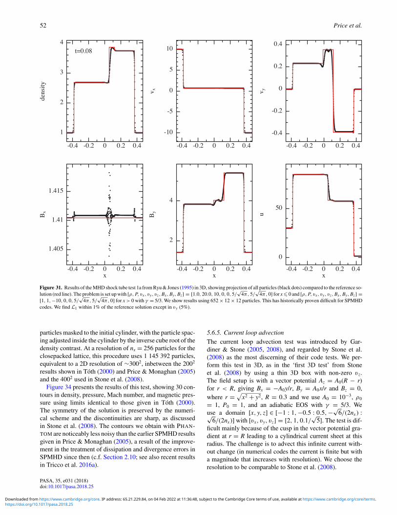
52 Price et al.

Figure 31. Results of the MHD shock tube test 1a from Ryu & Jones (1995) in 3D, showing projection of all particles (black dots) compared to the reference so-lution (red line). The problem is set up with [ρ, P, vx, vy, vz, Bx, By, Bz] = [1.0, 20.0, 10, 0, 0, 5/

√4π, 5/

√4π, 0] for x� 0 and [ρ, P, vx, vy, vz, Bx, By, Bz] =

[1, 1,−10, 0, 0, 5/√

4π, 5/√

4π, 0] for x > 0 with γ = 5/3. We show results using 652 × 12 × 12 particles. This has historically proven difficult for SPMHDcodes. We find L1 within 1% of the reference solution except in vy (5%).

particles masked to the initial cylinder, with the particle spac-ing adjusted inside the cylinder by the inverse cube root of thedensity contrast. At a resolution of nx = 256 particles for theclosepacked lattice, this procedure uses 1 145 392 particles,equivalent to a 2D resolution of ∼3002, inbetween the 2002

results shown in Tóth (2000) and Price & Monaghan (2005)and the 4002 used in Stone et al. (2008).

Figure 34 presents the results of this test, showing 30 con-tours in density, pressure, Mach number, and magnetic pres-sure using limits identical to those given in Tóth (2000).The symmetry of the solution is preserved by the numeri-cal scheme and the discontinuities are sharp, as discussedin Stone et al. (2008). The contours we obtain with PHAN-TOM are noticeably less noisy than the earlier SPMHD resultsgiven in Price & Monaghan (2005), a result of the improve-ment in the treatment of dissipation and divergence errors inSPMHD since then (c.f. Section 2.10; see also recent resultsin Tricco et al. 2016a).

5.6.5. Current loop advection

The current loop advection test was introduced by Gar-diner & Stone (2005, 2008), and regarded by Stone et al.(2008) as the most discerning of their code tests. We per-form this test in 3D, as in the ‘first 3D test’ from Stoneet al. (2008) by using a thin 3D box with non-zero v z.The field setup is with a vector potential Az = A0(R − r)for r < R, giving Bx = −A0y/r, By = A0x/r and Bz = 0,where r =

√x2 + y2, R = 0.3 and we use A0 = 10−3, ρ0

= 1, P0 = 1, and an adiabatic EOS with γ = 5/3. Weuse a domain [x, y, z] ∈ [−1 : 1,−0.5 : 0.5,−√

6/(2nx ) :√6/(2nx )] with [vx, vy, vz] = [2, 1, 0.1/

√5]. The test is dif-

ficult mainly because of the cusp in the vector potential gra-dient at r = R leading to a cylindrical current sheet at thisradius. The challenge is to advect this infinite current with-out change (in numerical codes the current is finite but witha magnitude that increases with resolution). We choose theresolution to be comparable to Stone et al. (2008).

PASA, 35, e031 (2018)doi:10.1017/pasa.2018.25






Phantom 53

Figure 32. Density in a z = 0 cross section of the Orszag-Tang vortex test performed in 3D. Results are shown at t = 0.5 (top) and t = 1 (bottom) at aresolution of 128 × 148 × 12, 256 × 296 × 12 and 512 × 590 × 12 particles (left to right). Compare e.g. to Figure 4 in Dai & Woodward (1994b) or Figure 22in Stone et al. (2008), while improvements in the SPMHD method over the last decade can be seen by comparing to Figure 14 in Price & Monaghan (2005).

Figure 33. Horizontal slices of pressure shown at t=0.5 in the Orszag–Tangvortex test. We show cuts along y = 0.3125 (top) and y = 0.4277 (bottom)in the z = 0 plane for three different numerical resolutions (see legend).

For SPMHD, this is mainly a test of the shock dissipa-tion and divergence cleaning terms, since in the absence ofthese terms the advection can be computed to machine pre-cision [c.f. 2D results shown in Rosswog & Price (2007)

and Figure 11 of Price (2012a), shown after one thousandcrossings of the computational domain]. Figure 35 shows theresults of this test in PHANTOM with 128 × 74 × 12 parti-cles after two box crossings, computed with all dissipationand divergence cleaning terms switched on, precisely as inthe previous tests including the shock tubes (Sections 5.6.2–5.6.4). Importantly, our implementation of artificial resistiv-ity (Section 2.10.6) guarantees that the dissipation is iden-tically zero when there is no relative velocity between theparticles, meaning that simple advection of the current loopis not affected by numerical resistivity. However, the problemremains sensitive to the divergence cleaning (Section 2.10.2),in particular to any spurious divergence of B that is measuredby the SPMHD divergence operator, (174). For this reason,the results using the quintic kernel, (19), are substantiallybetter than those using the cubic spline, because the initialmeasurement of ∇ · B is smaller and so the evolution is lessaffected by the divergence cleaning.

5.6.6. MHD blast wave

The MHD blast wave problem consists of an over-pressurisedcentral region that expands preferentially along the strongmagnetic field lines. Our setup uses the 3D initial condi-tions of Stone et al. (2008), which follows from the work of

PASA, 35, e031 (2018)doi:10.1017/pasa.2018.25






54 Price et al.

Figure 34. Density, pressure, Mach number, and magnetic pressure shown in a z = 0 cross section at t = 0.15 in the3D MHD rotor problem, using nx = 256, equivalent to ∼3002 resolution elements in 2D. The plots show 30 contourswith limits identical to those given by Tóth (2000); 0.483 < ρ < 12.95, 0.0202 < P < 2.008, 0 < |v |/cs < 1.09, and0 < 1

2 B2 < 2.642.

Londrillo & Del Zanna (2000) and Balsara & Spicer (1999).For a recent application of SPMHD to this problem, seeTricco & Price (2012) and Tricco et al. (2016a). Set in aperiodic box [x, y, z] ∈ [− 0.5, 0.5], the fluid has uniformρ = 1 and B = [10/

√2, 0, 10/

√2]. The pressure is set to P

= 1, using γ = 1.4, except for a region in the centre of ra-dius R = 0.125 which has its pressure increased to P = 100.This yields initial plasma beta β = 2 inside the blast and β

= 0.02 outside. The particles are arranged on a close-packedtriangular lattice using nx = 256.

Figure 36 shows slices through y = 0 of density, pressure,magnetic energy density, and kinetic energy density, whichmay be directly compared to results in Gardiner & Stone(2008). The shock positions and overall structure of the blastwave in all four variables show excellent agreement with theresults shown in their paper. The main difference is that theirsolution appears less smoothed, suggesting that the overallnumerical dissipation is lower in ATHENA.

5.6.7. Balsara–Kim supernova-driven turbulence

We reproduce the ‘test problem’ of Balsara & Kim (2004)(hereafter BK04) modelling supernova-driven turbulence inthe interstellar medium. BK04 used this test to argue stronglyagainst the use of divergence cleaning for problems involv-ing strong shocks. Specifically, they compared three differentdivergence cleaning schemes against a constrained transportmethod, finding that divergence cleaning was unusable forsuch problems, with all three divergence cleaning schemesproducing strong temporal fluctuations in magnetic energyduring the growth phase of the supernova-driven dynamo.The problems were attributed to issues with the non-localityof divergence cleaning.

We follow the setup in BK04 as closely as possible, but sev-eral issues make a direct comparison difficult. Chief amongthese is their use of a physical ISM cooling prescription. Weimplement a similar algorithm (Section 2.14), but our coolingprescription is not identical (e.g. our implementation includes

PASA, 35, e031 (2018)doi:10.1017/pasa.2018.25






Phantom 55

Figure 35. Magnitude of the current density |∇ × B| in the current loop ad-vection test performed in 3D, showing comparing the initial conditions (top)to the result after two (middle) and five (bottom) crossings of the box, using128 × 74 × 12 particles. Full dissipation, shock capturing, and divergencecleaning terms were applied for this test, without which the advection is ex-act to machine precision. The advection is affected mainly by the divergencecleaning acting on the outer (infinite) current sheet.

live chemistry and thus the possibility for a cold phase of theISM, which theirs does not). Second, they give the setup pa-rameters for the problem in computational units, but the useof ISM cooling requires the physical units of the problem tobe specified. Since these are not stated in their paper, one mustguess the units by reading descriptions of the same problemin physical units given in Kim, Balsara, & Mac Low (2001),Balsara et al. (2004), and Mac Low et al. (2005).

We set up the problem as follows. Particles are initialisedon a close-packed lattice in a periodic box with x, y, z ∈ [−0.1, 0.1], with ρ = 1 and the initial thermal pressure set toP = 0.3 (all in code units, as specified in BK04). We infer alength unit of kpc since this is described as a ‘200 pc3 box’in their other papers. We employ an adiabatic EOS with γ

= 5/3 and turn on interstellar cooling and chemistry in thecode with default initial abundances (i.e. atomic Hydrogeneverywhere). We choose the mass unit such that a densityof 2.3 × 10−23 g cm−3, as described in Kim et al. (2001),corresponds to ρ = 1 in code units as described in BK04.Finally, we set the time unit such that G = 1 in code units (acommon choice, even though gravity is not involved in theproblem). We compute the problem using resolutions of 64× 74 × 78 particles and 128 × 148 × 156 particles.

Supernovae are injected into the simulation every 0.00125in code units at the positions listed in Table 1 of BK04. We in-fer this to correspond to the ‘12 × Galactic’ rate described inBalsara et al. (2004), i.e. 12 times faster than 1 per 1.26 Myr.We inject supernovae following the description in BK04 bysetting the pressure to P = 13649.6 on particles within a dis-tance of 0.005 code units from the injection site (correspond-ing to a radius of 5 pc in physical units). Our choice of unitsmeans that this corresponds to an energy injection within afew percent of 1051 ergs in physical units, corresponding tothe description given in their other papers. However, this isonly true if the density equals the initial value, since BK04specify pressure rather than the energy. We follow the de-scription in BK04 (i.e. we set the pressure), even though thisgives an energy not equal to 1051 ergs if injected in a low orhigh density part of the computational domain.

The initial magnetic field is uniform in the x-direction withBx = 0.056117, as stated in BK04. We could not reconcilethis with the magnetic energy plotted in their paper, whichshow an initial magnetic energy of 10−6. Nor could we rec-oncile this with the statement in Balsara et al. (2004) that‘the magnetic energy is 10−6 times smaller than the thermalenergy’. So any comparison is approximate. Nevertheless,BK04 state that the problems caused by divergence cleaningare not dependent on specific details of the implementation.

Figure 37 shows the evolution of the column density in thelowest resolution calculation using 64 × 74 × 78 particles.The combination of supernovae injection and cooling drivesturbulence and significant structure in the density field.

To specifically address the issues found by BK04,Figure 38 shows a cross-section slice of the magnetic pres-sure at a time similar to the one shown in Figure 3 of BK04(they do not indicate which slice they plotted, we chose z= 0.0936). The magnetic pressure in the interior of the su-pernovae shells is smooth, and does not display any of thelarge-scale artefacts of the type found in their paper.

Figure 39 shows the time evolution of the magnetic energyin the low-resolution calculation. The magnetic energy risesmonotonically up to t ≈ 0.02 before the magnetic energy sat-urates, similar to what was found by BK04 for their staggeredmesh/constrained transport scheme (compare with Figure 2in their paper). There are no large temporal fluctuations in themagnetic energy of the kind they report for their divergencecleaning methods.

In summary, the results we obtain for the magnetic fieldenergy and structure within supernova-driven turbulence inthe interstellar medium match closest the constrained trans-port result of BK04. There is no evidence that our simulationsexperience the numerical issues encountered by BK04 withtheir divergence cleaning schemes, suggesting that the prob-lems they reported are primarily code dependent rather thanbeing fundamental. The most probable reason our results areof the same quality as BK04’s constrained transport result isour use of constrained divergence cleaning, which guaran-tees that energy removed from the magnetic field is negativedefinite. A follow-up study to examine this in more depth

PASA, 35, e031 (2018)doi:10.1017/pasa.2018.25






56 Price et al.

t=0.02 P

|B|2/2 |v|2/2

Figure 36. Slices through y = 0 for the MHD blast wave problem showing density (top left), gas pressure (top right),magnetic energy density (bottom left), and kinetic energy density (bottom right). The plot limits are ρ ∈ [0.19, 2.98],P ∈ [1, 42.4], [25.2, 64.9] for the magnetic energy density and [0, 33.1] for the kinetic energy density. These are directlycomparable to Figure 8 in Gardiner & Stone (2008).

would be worthwhile. For our present purposes, we can con-clude that our divergence cleaning algorithm is sufficientlyrobust—even in ‘real-world’ problems—to be useful in prac-tice (see also Section 6.3).

5.7. Non-ideal MHD

The following tests demonstrate the non-ideal MHD algo-rithms (Section 2.11). We adopt periodic boundary condi-tions for both tests, initialising the particles on a close-packedlattice with an isothermal EOS, P = c2

s ρ, and using the C4

Wendland kernel.

5.7.1. Wave damping test

To test ambipolar diffusion in the strong coupling approxi-mation, we follow the evolution of decaying Alfvén waves,as done in (e.g.) Choi, Kim, & Wiita (2009) and Wurster et al.(2014).

In arbitrary units, the initial conditions are a box of sizeLx ×

√3

2 Lx ×√

62 Lx with Lx = 1, a density of ρ = 1, magnetic

field of B = B0x with B0 = 1, sound speed of cs = 1, andvelocity of v = v0 sin(kx)z, where k = 2π /Lx is the wavenumber, and v0 = 0.01vA, where vA is the Alfvén velocity. Weadopt an ambipolar diffusion coefficient of ηAD = 0.01v2

A.All artificial dissipation terms are turned off. We use nx =128 particles.

The solution to the dispersion relation for Alfvén waves(Balsara 1996) is

ω2 + ηADk2ωi − v2Ak2 = 0, (323)

where ω = ωR + ωIi is the complex angular frequency of thewave, giving a damped oscillation in the form

h(t ) = h0 |sin (ωRt )| eωIt . (324)

In our test, h(t) corresponds the root mean square of the mag-netic field in the z-direction,

⟨B2

z

⟩1/2, and h0 = v0B0/(vA

√2).

PASA, 35, e031 (2018)doi:10.1017/pasa.2018.25






Phantom 57

Figure 37. Balsara–Kim supernova-driven turbulence, showing column density at three different times at a resolution of 64 × 74 × 78 particles. Supernovaeare injected every 0.00125 in code units, leading to a series of interacting blast waves. Interstellar chemistry and cooling is turned on, producing a densefilaments in a turbulent interstellar medium.

Figure 38. Cross-section slice of magnetic pressure at t = 0.006 in theBalsara–Kim supernova-driven turbulence test using 128 × 148 × 156 par-ticles. No large-scale artefacts in magnetic energy are visible, indicating thatthe simulation is not corrupted by divergence cleaning.

Figure 40 shows the time evolution of⟨B2

z

⟩1/2to t = 5 for

both the numerical results (blue line) and the analytic solution(red line). At the end of the test, the L2 error is 7.5 × 10−5

(evaluated at intervals of dt = 0.01), demonstrating closeagreement between the numerical and analytical results.

Given that, by design, there is motion of the particles andthat we have excluded artificial dissipation, the particles tendto ‘break’ from the initial lattice. For both the M6 quintickernel and the C4 Wendland kernel on a cubic lattice, the par-ticles fall off the lattice at t ≈ 0.75. Prior to this, however, theL2 error is smaller than that calculated using the C4 Wend-

Time

Em

ag

0 0.01 0.02 0.03

10-5

10-4

10-3

64 x 74 x 78

Figure 39. Magnetic energy as a function of time in the Balsara–Kimsupernova-driven turbulence problem. The magnetic energy increases mono-tonically by approximately an order of magnitude before reaching its satu-ration value at t ≈ 0.02. There are no spurious spikes in magnetic energycaused by divergence cleaning, in contrast to what was found by Balsara &Kim (2004).

land kernel and a close-packed lattice, thus there is a tradeoff between accuracy and long-term stability.

5.7.2. Standing shock

To test the Hall effect, we compare our solutions against the1D isothermal steady-state equations for the strong Hall ef-fect regime. The numerical solution to this problem is givenin Falle (2003) and O’Sullivan & Downes (2006), and alsosummarised in Appendix C1.2 of Wurster et al. (2016).

The left- and right-hand side of the shock are initialisedwith (ρ0, vx, 0, vy, 0, vz, 0, Bx, 0, By, 0, Bz, 0) = (1.7942,−0.9759, −0.6561, 0.0, 1.0, 1.74885, 0.0) and (1.0, −1.751,

PASA, 35, e031 (2018)doi:10.1017/pasa.2018.25






58 Price et al.

0

0.001

0.002

0.003

0.004

0.005

0.006

0.007

0 1 2 3 4 5

<B

z2 >1/

2

Time

AnalyticalNumerical

Figure 40. Wave damping test showing the decay of Alfvén waves in thepresence of ambipolar diffusion, using the coefficient ηAD = 0.01v2

A. TheL2 error between the analytic and numerical solution is 7.5 × 10−5.

0.0, 0.0, 1.0, 0.6, 0.0), respectively, with the discontinuity at x= 0. We use boundary particles at the x-boundary, supersed-ing the periodicity in this direction. To replicate inflowingboundary conditions in the x-direction, when required, theinitial domain of interest xl < x < xr is automatically adjustedto x′

l < x < x′r , where x′

r = xr − v0tmax, where tmax is the endtime of the simulation. Note that for inflowing conditions,xr and v0 will have opposite signs. Thus, at the end of thesimulation, the entire range of interest will still be populatedwith particles.

The non-ideal MHD coefficients are ηOR = 1.12 × 10−12,ηHE = −3.53 × 10−2B, and ηAD = 7.83 × 10−3v2

A. We in-clude all artificial dissipation terms using their default set-tings. We initialise 512 × 14 × 15 particles in x < 0 and 781× 12 × 12 particles in x� 0, with the domain extending fromxl = x′

l = −2 to xr = 2 with x′r = 3.75.

Figure 41 shows vx and By for both the numerical andanalytical results, which agree to within 3% at any givenposition.

On the left-hand side of the shock interface, the numericalresults are lower than the analytical solution because of theartificial dissipation terms, which are required to properlymodel a shock. These results do not depend on either thekernel choice or the initial particle lattice configuration.

5.8. Self-gravity

5.8.1. Polytrope

The simplest test of self-gravity is to model a sphericalpolytrope in hydrostatic equilibrum. Similar tests have beenshown for SPH codes dating back to the original papers ofGingold & Monaghan (1977, 1978, 1980). Modern calcula-tions have used these simple models in more complex ap-plications, ranging from common envelope evolution (Iaconiet al. 2017) to tidal disruption events (Coughlin & Nixon

-1.8

-1.6

-1.4

-1.2

-1.0

-0.8

v x

AnalyticalNumerical

0.0

0.4

0.8

1.2

1.6

-0.25 0.00 0.25 0.50 0.75

By

x

Figure 41. Hall-dominated standing shock using ηOR = 1.12 × 10−12, ηHE

=−3.53 ×10−2B, and ηAD = 7.83 × 10−3v2A. The numerical and analytical

results agree to within 3% everywhere.

Figure 42. Polytrope static structure using 106 particles (black), comparedto the exact solution (red), shown at t = 100.

2015; Coughlin et al. 2016b, 2016a; Bonnerot et al. 2016,2017).

The EOS is P = Kργ , with γ = 1 + 1/n where n is thepolytropic index. The exact hydrostatic solution is given by

γ K

4πG (γ − 1)

d2

dr2

(rργ−1

)+ rρ = 0. (325)

Our initial setup uses a solution scaled to a radius R = 1, for apolytropic index of n = 3/2, corresponding to γ = 5/3, with K= 0.4244. We solve (325) numerically. We place the particlesinitially on a hexagonal close-packed lattice, truncated to aradius of R = 1, which we then stretch map (see Section 3.2)such that the initial radial density profile matches the exactsolution.

The relaxation time depends on the initial density profileand on how far the initial particle configuration is from equi-

PASA, 35, e031 (2018)doi:10.1017/pasa.2018.25






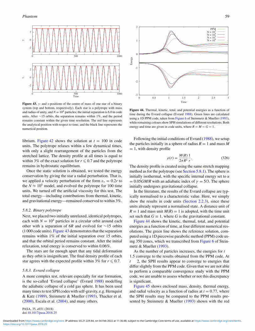
Phantom 59

Figure 43. y- and x-positions of the centre of mass of one star of a binarysystem (top and bottom, respectively). Each star is a polytrope with massand radius of unity, and N = 104 particles; the initial separation is 6.0 in codeunits. After ∼15 orbits, the separation remains within 1%, and the periodremains constant within the given time resolution. The red line representsthe analytical position with respect to time, and the black line represents thenumerical position.

librium. Figure 42 shows the solution at t = 100 in codeunits. The polytrope relaxes within a few dynamical times,with only a slight rearrangement of the particles from thestretched lattice. The density profile at all times is equal towithin 3% of the exact solution for r � 0.7 and the polytroperemains in hydrostatic equilibrium.

Once the static solution is obtained, we tested the energyconservation by giving the star a radial perturbation. That is,we applied a velocity perturbation of the form v r = 0.2r tothe N ≈ 105 model, and evolved the polytrope for 100 timeunits. We turned off the artificial viscosity for this test. Thetotal energy—including contributions from thermal, kinetic,and gravitational energy—remained conserved to within 3%.

5.8.2. Binary polytrope

Next, we placed two initially unrelaxed, identical polytropes,each with N = 104 particles in a circular orbit around eachother with a separation of 6R and evolved for ∼15 orbits(1 000 code units). Figure 43 demonstrates that the separationremains within 1% of the initial separation over 15 orbits,and that the orbital period remains constant. After the initialrelaxation, total energy is conserved to within 0.06%.

The stars are far enough apart that any tidal deformationas they orbit is insignificant. The final density profile of eachstar agrees with the expected profile within 3% for r � 0.7.

5.8.3. Evrard collapse

A more complex test, relevant especially for star formation,is the so-called ‘Evrard collapse’ (Evrard 1988) modellingthe adiabatic collapse of a cold gas sphere. It has been usedmany times to test SPH codes with self-gravity, e.g. Hernquist& Katz (1989), Steinmetz & Mueller (1993), Thacker et al.(2000), Escala et al. (2004), and many others.

-3

-2

-1

0

1

2

0 0.5 1 1.5 2 2.5 3

Ene

rgy

Time

PPMN = 103

N = 104

N = 105

N = 106

Figure 44. Thermal, kinetic, total, and potential energies as a function oftime during the Evrard collapse (Evrard 1988). Green lines are calculatedusing a 1D PPM code, taken from Figure 6 of Steinmetz & Mueller (1993),while remaining colours show SPH simulations of different resolutions. Bothenergy and time are given in code units, where R = M = G = 1.

Following the initial conditions of Evrard (1988), we setupthe particles initially in a sphere of radius R = 1 and mass M= 1, with density profile

ρ(r) = M(R)

2πR2

1

r. (326)

The density profile is created using the same stretch mappingmethod as for the polytrope (see Section 5.8.1). The sphere isinitially isothermal, with the specific internal energy set to u= 0.05GM/R with an adiabatic index of γ = 5/3. The sphereinitially undergoes gravitational collapse.

In the literature, the results of the Evrard collapse are typ-ically normalised to a characteristic value. Here, we simplyshow the results in code units (Section 2.2.3), since theseunits already represent a normalised state. A distance unit ofR = 1 and mass unit M(R) = 1 is adopted, with the time unitset such that G ≡ 1, where G is the gravitational constant.

Figure 44 shows the kinetic, thermal, total, and potentialenergies as a function of time, at four different numerical res-olutions. The green line shows the reference solution, com-puted using a 1D piecewise parabolic method (PPM) code us-ing 350 zones, which we transcribed from Figure 6 of Stein-metz & Mueller (1993).

As the number of particles increases, the energies for t �1.5 converge to the results obtained from the PPM code. Att � 2, the SPH results appear to converge to energies thatdiffer slightly from the PPM code. Given that we are not ableto perform a comparable convergence study with the PPMcode, we are unable to assess whether or not this discrepancyis significant.

Figure 45 shows enclosed mass, density, thermal energy,and radial velocity as a function of radius at t = 0.77, wherethe SPH results may be compared to the PPM results pre-sented by Steinmetz & Mueller (1993) shown with the red

PASA, 35, e031 (2018)doi:10.1017/pasa.2018.25






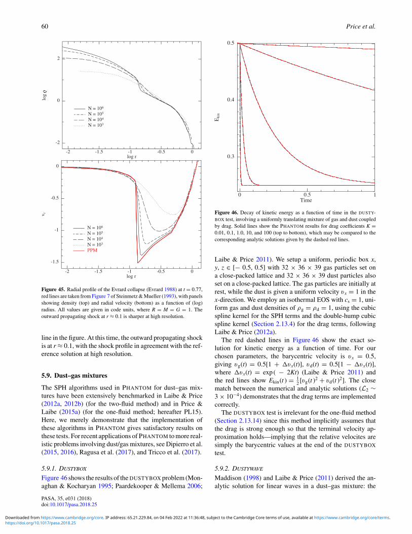
60 Price et al.

Figure 45. Radial profile of the Evrard collapse (Evrard 1988) at t = 0.77,red lines are taken from Figure 7 of Steinmetz & Mueller (1993), with panelsshowing density (top) and radial velocity (bottom) as a function of (log)radius. All values are given in code units, where R = M = G = 1. Theoutward propagating shock at r ≈ 0.1 is sharper at high resolution.

line in the figure. At this time, the outward propagating shockis at r ≈ 0.1, with the shock profile in agreement with the ref-erence solution at high resolution.

5.9. Dust–gas mixtures

The SPH algorithms used in PHANTOM for dust–gas mix-tures have been extensively benchmarked in Laibe & Price(2012a, 2012b) (for the two-fluid method) and in Price &Laibe (2015a) (for the one-fluid method; hereafter PL15).Here, we merely demonstrate that the implementation ofthese algorithms in PHANTOM gives satisfactory results onthese tests. For recent applications of PHANTOM to more real-istic problems involving dust/gas mixtures, see Dipierro et al.(2015, 2016), Ragusa et al. (2017), and Tricco et al. (2017).

5.9.1. DUSTYBOX

Figure 46 shows the results of the DUSTYBOX problem (Mon-aghan & Kocharyan 1995; Paardekooper & Mellema 2006;

Figure 46. Decay of kinetic energy as a function of time in the DUSTY-BOX test, involving a uniformly translating mixture of gas and dust coupledby drag. Solid lines show the PHANTOM results for drag coefficients K =0.01, 0.1, 1.0, 10, and 100 (top to bottom), which may be compared to thecorresponding analytic solutions given by the dashed red lines.

Laibe & Price 2011). We setup a uniform, periodic box x,y, z ∈ [− 0.5, 0.5] with 32 × 36 × 39 gas particles set ona close-packed lattice and 32 × 36 × 39 dust particles alsoset on a close-packed lattice. The gas particles are initially atrest, while the dust is given a uniform velocity vx = 1 in thex-direction. We employ an isothermal EOS with cs = 1, uni-form gas and dust densities of ρg = ρd = 1, using the cubicspline kernel for the SPH terms and the double-hump cubicspline kernel (Section 2.13.4) for the drag terms, followingLaibe & Price (2012a).

The red dashed lines in Figure 46 show the exact so-lution for kinetic energy as a function of time. For ourchosen parameters, the barycentric velocity is vx = 0.5,giving vg(t) = 0.5[1 + �vx(t)], vd(t) = 0.5[1 − �vx(t)],where �vx(t) = exp ( − 2Kt) (Laibe & Price 2011) andthe red lines show Ekin(t ) = 1

2 [vg(t )2 + vd(t )2]. The closematch between the numerical and analytic solutions (L2 ∼3 × 10−4) demonstrates that the drag terms are implementedcorrectly.

The DUSTYBOX test is irrelevant for the one-fluid method(Section 2.13.14) since this method implicitly assumes thatthe drag is strong enough so that the terminal velocity ap-proximation holds—implying that the relative velocites aresimply the barycentric values at the end of the DUSTYBOX

test.

5.9.2. DUSTYWAVE

Maddison (1998) and Laibe & Price (2011) derived the an-alytic solution for linear waves in a dust–gas mixture: the

PASA, 35, e031 (2018)doi:10.1017/pasa.2018.25






Phantom 61

Figure 47. Velocity of gas (solid) and dust (circles) at t = 4.5 in the DUSTYWAVE test, using the two-fluid method (left; with 64 × 12 × 12 gas particles,64 × 12 × 12 dust particles) and the one-fluid method (right; with 64 × 12 × 12 mixture particles) and a dust-to-gas ratio of unity. Panels show results withK = 0.5, 5, 50, and 500 (top to bottom), corresponding to the stopping times indicated. The two-fluid method is accurate when the stopping time is long (topthree panels in left figure) but requires h � csts to avoid overdamping (bottom two panels on left; Laibe & Price 2012a). The one-fluid method should be usedwhen the stopping time is short (right figure).

‘DUSTYWAVE’ test. The corresponding dispersion relation isgiven by (Maddison 1998; Laibe & Price 2011, 2012a)

ω3 + iK

(1

ρg+ 1

ρd

)ω2 − c2

s k2ω − iKk2c2

s

ρd= 0, (327)

which can be more clearly expressed as

(ω2 − c2s k2) + i

ωts(ω2 − c2

s k2) = 0, (328)

where cs = cs(1 + ρd/ρg)−1/2 is the modified sound speed(e.g. Miura & Glass 1982). This demonstrates the two im-portant limits: (i) ts → ∞, giving undamped sound waves inthe gas and (ii) ts → 0, giving undamped sound waves in themixture propagating at the modified sound speed. In betweenthese limits, the mixture is dissipative and waves are dampedby the imaginary term. This is seen in the analytic solutionsshown in Figure 47.

Two-fluid. We perform this test first with the two-fluid al-gorithm, using 64 × 12 × 12 gas particles and 64 × 12 × 12dust particles set up on a uniform, close-packed lattice in aperiodic box with x ∈ [− 0.5, 0.5] and the y and z boundariesset to correspond to 12 particle spacings on the chosen lattice.The wave is set to propagate along the x-axis with vg = vd

= Asin (2πx), ρ = ρ0[1 + Asin (2πx)] with ρ0 = 1 and A= 10−4. The density perturbation is initialised using stretchmapping (Section 3.2; see also Appendix B in Price & Mon-aghan 2004b). We perform this test using an adiabatic EOSwith cs, 0 = 1. We adopt a simple, constant K drag prescrip-tion, choosing K = 0.5, 5, 50, and 500 such that the stopping

time given by (236) is a multiple of the wave period (ts = 1,0.1, 0.01, and 0.001, respectively).

The left panels in Figure 47 show the results of this testusing the two-fluid method, showing velocity in each phasecompared to the analytic solution after 4.5 wave periods (thetime is chosen to give a phase offset between the phases).For stopping times ts � 0.1, the numerical solution matchesthe analytic solution to within 4%. For short stopping times,Laibe & Price (2012a) showed that the resolution criterionh � csts needs to be satisfied to avoid overdamping of themixture. For the chosen number of particles, the smoothinglength is h = 0.016, implying in this case that the criterion isviolated when ts � 0.016. This is evident from the lower twopanels in Figure 47, where the numerical solution is over-damped compared to the analytic solution.

This problem is not unique to SPH codes, but represents afundamental limitation of two-fluid algorithms in the limit ofshort stopping times due to the need to resolve the physicalseparation between the phases (which becomes ever smalleras ts decreases) when they are modelled with separate setsof particles (or with a grid and a physically separate set ofdust particles). The need to resolve a physical length scaleresults in first-order convergence of the algorithm in the limitof short stopping times, as already noticed by Miniati (2010)in the context of grid-based codes. The problem is less severewhen the dust fraction is small (Lorén-Aguilar & Bate 2014),but is difficult to ameliorate fully.

One-fluid. The limit of short stopping time (small grains)is the limit in which the mixture is well described by the

PASA, 35, e031 (2018)doi:10.1017/pasa.2018.25






62 Price et al.

one-fluid formulation in the terminal velocity approximation(Section 2.13.12). To compare and contrast the two methodsfor simulating dust in PHANTOM, the right half of Figure 47shows the results of the DUSTYWAVE test computed with theone-fluid method. To perform this test, we set up a singleset of 64 × 12 × 12 ‘mixture’ particles placed on a uniformclosepacked lattice, with an initially uniform dust fraction ε

= 0.5. The particles are given a mass corresponding to thecombined mass of the gas and dust, with the density pertur-bation set as previously.

The one-fluid solution is accurate precisely where the two-fluid method is inaccurate, and vice-versa. For short stop-ping times (ts = 0.001; bottom row) the numerical solu-tion is within 1.5% of the analytic solution, compared toerrors greater than 60% for the two-fluid method (left fig-ure). For long stopping times (ts � 1; top two rows), theone-fluid method is both inaccurate and slow, but this is pre-cisely the regime in which the two-fluid method (left figure)is explicit and therefore cheap. Thus, the two methods arecomplementary.

5.9.3. Dust diffusion

A simple test of the one-fluid dust diffusion algorithm is givenby PL15. For this test, we set up the particles on a uniformcubic lattice in a 3D periodic box x, y, z ∈ [− 0.5, 0.5] using 32× 32 × 32 particles with an initial dust fraction set accordingto

ε(r, 0) =

⎧⎪⎨⎪⎩

ε0

[1 −

(r

rc

)2]

, r < rc,

0, elsewhere,

(329)

with ε0 = 0.1 and rc = 0.25. We then evolve the dust diffusionequation, (272), discretised according to (279), while settingthe acceleration and thermal energy evolution to zero andassuming P = ρ, with the stopping time set to a constantts = 0.1 and the computational timestep set to �t = 0.05.Figure 48 shows the evolution of the dust fraction ε ≡ ρd/ρ asa function of radius at various times, showing the projection ofall particles in the box (points) compared to the exact solution(red lines) at t = 0.0, 0.1, 0.3, 1.0, and 10.0 (top to bottom).The solution shows a close match to the analytic solution,with agreement to within 0.3% of the analytic solution at alltimes.

5.9.4. Dust settling

We perform the dust settling test from PL15 in order to di-rectly compare the PHANTOM solutions to those produced inPL15 with the NDSPMHD code. To simplify matters, we donot consider rotation but simply adapt the 2D problem to 3Dby using a thin Cartesian box (as for several of the MHD testsin Section 5.6). Our setup follows PL15, considering a sliceof a protoplanetary disc at R0 = 50 au in the r–z plane (corre-sponding to our x and y Cartesian coordinates, respectively)

Figure 48. Dust diffusion test from Price & Laibe (2015a), showing theevolution of the dust fraction on the particles (black dots) as a function ofradius at six different times (top to bottom), which may be compared to theanalytic solution given by the red lines.

with density in the ‘vertical’ direction (y) given by

ρ(y) = ρ0 exp

(−y2

2H 2

), (330)

where we choose H/R0 = 0.05 giving H = 2.5 au. We usean isothermal EOS with sound speed cs ≡ H�, where � ≡√

GM/R30, corresponding to an orbital time torb ≡ 2π /� ≈

353 yr. We adopt code units with a distance unit of 10 au,mass in solar masses, and time units such that G = 1, givingan orbital time of ≈70.2 in code units. We apply an externalacceleration in the form

aext = − GMy√R2

0 + y2, (331)

where G = M = 1 in code units.The particles are placed initially on a close-packed lat-

tice using 32 × 110 × 24 = 84 480 particles in the domain[x, y, z] ∈ [±0.25,±3H,±√

3/128]. We then use the stretchmapping routine (Section 3.2) to give the density profile ac-cording to (330). We set the mid-plane density to 10−3 incode units, or ≈6 × 10−13g cm−3. The corresponding par-ticle mass in code units is 1.13 × 10−9. We use periodicboundaries, with the boundary in the y direction set at ±10Hto avoid periodicity in the vertical direction.

Following the procedure in PL15, we relax the densityprofile by evolving for 15 orbits with gas only with damp-ing switched on. We then restart the calculation with either(i) a dust fraction added to each particle (one-fluid) or (ii) acorresponding set of dust particles duplicated from the gasparticles (two-fluid). For the dust, we assume 1-mm grainswith an Epstein drag prescription, such that the stopping timeis given by (250). Since �v is not available when comput-ing ts with the one-fluid method, we set the factor f = 1 in(250) when using this method (this is a valid approximationsince by definition �v is small when the one-fluid method

PASA, 35, e031 (2018)doi:10.1017/pasa.2018.25






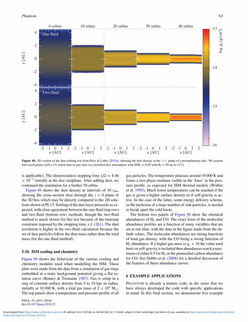
Phantom 63

Figure 49. 3D version of the dust settling test from Price & Laibe (2015a), showing the dust density in the ‘r–z’ plane of a protoplanetary disc. We assumemm-sized grains with a 1% initial dust-to-gas ratio in a stratified disc atmosphere with H/R0 = 0.05 with R0 = 50 au in (331).

is applicable). The dimensionless stopping time ts� = 8.46× 10−3 initially at the disc midplane. After adding dust, wecontinued the simulation for a further 50 orbits.

Figure 49 shows the dust density at intervals of 10 torb,showing the cross-section slice through the z = 0 plane ofthe 3D box which may be directly compared to the 2D solu-tions shown in PL15. Settling of the dust layer proceeds as ex-pected, with close agreement between the one-fluid (top row)and two-fluid (bottom row) methods, though the two-fluidmethod is much slower for this test because of the timestepconstraint imposed by the stopping time, c.f. (261). The dustresolution is higher in the two-fluid calculation because theset of dust particles follow the dust mass rather than the totalmass (for the one-fluid method).

5.10. ISM cooling and chemistry

Figure 50 shows the behaviour of the various cooling andchemistry modules used when modelling the ISM. Theseplots were made from the data from a simulation of gas ringsembedded in a static background potential giving a flat ro-tation curve (Binney & Tremaine 1987). Gas is setup in aring of constant surface density from 5 to 10 kpc in radius,initially at 10 000 K, with a total gas mass of 2 × 109 M�.The top panels show a temperature and pressure profile of all

gas particles. The temperature plateaus around 10 000 K andforms a two-phase medium visible in the ‘knee’ in the pres-sure profile, as expected for ISM thermal models (Wolfireet al. 1995). Much lower temperatures can be reached if thegas is given a higher surface density or if self-gravity is ac-tive. In the case of the latter, some energy delivery scheme,or the inclusion of a large number of sink particles, is neededto break apart the cold knots.

The bottom two panels of Figure 50 show the chemicalabundances of H2 and CO. The exact form of the molecularabundance profiles are a function of many variables that areset at run time, with the data in the figure made from the de-fault values. The molecular abundances are strong functionsof total gas density, with the CO being a strong function ofH2 abundance. If a higher gas mass (e.g. × 10 the value usedhere) or self-gravity is included then abundances reach a max-imum of either 0.5 for H2 or the primordial carbon abundancefor CO. See Dobbs et al. (2008) for a detailed discussion ofthe features of these abundance curves.

6 EXAMPLE APPLICATIONS

PHANTOM is already a mature code, in the sense that wehave always developed the code with specific applicationsin mind. In this final section, we demonstrate five example

PASA, 35, e031 (2018)doi:10.1017/pasa.2018.25






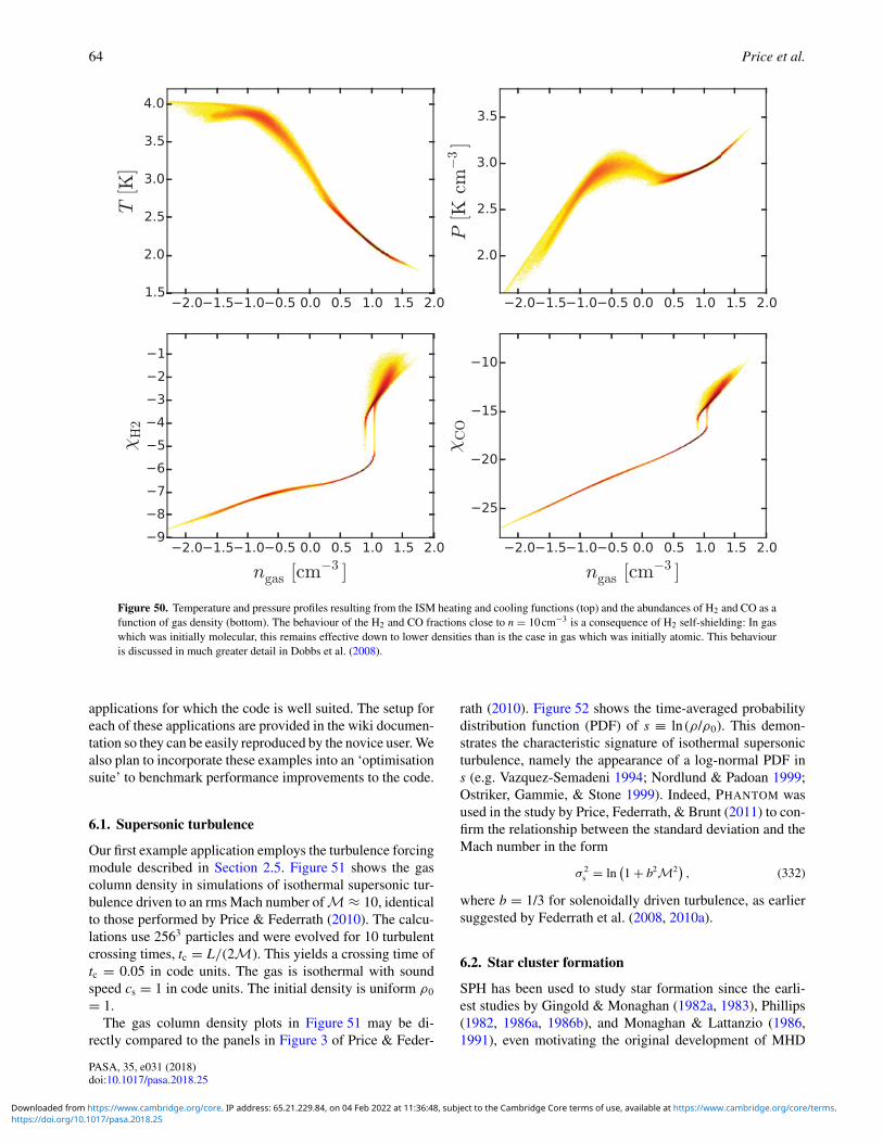
64 Price et al.

Figure 50. Temperature and pressure profiles resulting from the ISM heating and cooling functions (top) and the abundances of H2 and CO as afunction of gas density (bottom). The behaviour of the H2 and CO fractions close to n = 10 cm−3 is a consequence of H2 self-shielding: In gaswhich was initially molecular, this remains effective down to lower densities than is the case in gas which was initially atomic. This behaviouris discussed in much greater detail in Dobbs et al. (2008).

applications for which the code is well suited. The setup foreach of these applications are provided in the wiki documen-tation so they can be easily reproduced by the novice user. Wealso plan to incorporate these examples into an ‘optimisationsuite’ to benchmark performance improvements to the code.

6.1. Supersonic turbulence

Our first example application employs the turbulence forcingmodule described in Section 2.5. Figure 51 shows the gascolumn density in simulations of isothermal supersonic tur-bulence driven to an rms Mach number of M ≈ 10, identicalto those performed by Price & Federrath (2010). The calcu-lations use 2563 particles and were evolved for 10 turbulentcrossing times, tc = L/(2M). This yields a crossing time oftc = 0.05 in code units. The gas is isothermal with soundspeed cs = 1 in code units. The initial density is uniform ρ0

= 1.The gas column density plots in Figure 51 may be di-

rectly compared to the panels in Figure 3 of Price & Feder-

rath (2010). Figure 52 shows the time-averaged probabilitydistribution function (PDF) of s ≡ ln (ρ/ρ0). This demon-strates the characteristic signature of isothermal supersonicturbulence, namely the appearance of a log-normal PDF ins (e.g. Vazquez-Semadeni 1994; Nordlund & Padoan 1999;Ostriker, Gammie, & Stone 1999). Indeed, PHANTOM wasused in the study by Price, Federrath, & Brunt (2011) to con-firm the relationship between the standard deviation and theMach number in the form

σ 2s = ln

(1 + b2M2

), (332)

where b = 1/3 for solenoidally driven turbulence, as earliersuggested by Federrath et al. (2008, 2010a).

6.2. Star cluster formation

SPH has been used to study star formation since the earli-est studies by Gingold & Monaghan (1982a, 1983), Phillips(1982, 1986a, 1986b), and Monaghan & Lattanzio (1986,1991), even motivating the original development of MHD

PASA, 35, e031 (2018)doi:10.1017/pasa.2018.25






Phantom 65

Figure 51. Gas column density in PHANTOM simulations of driven, isothermal, supersonic turbulence at Mach 10, similar to the calculations performedby Price & Federrath (2010). We show the numerical solutions at t = 1, 2, and 3 crossing times (left to right, respectively). The colour scale is logarithmicbetween 10−1 and 10 in code units.

Figure 52. Time-averaged PDF of s = ln (ρ/ρ0) for supersonic Mach 10turbulence, with the shaded region representing the standard deviation ofthe averaging. The PDF is close to a log-normal distribution, shown by thedashed red line.

in SPH by Phillips & Monaghan (1985). The study by Bateet al. (2003) represented the first simulation of ‘large-scale’star cluster formation, resolved to the opacity limit for frag-mentation (Rees 1976; Low & Lynden-Bell 1976). This wasenabled by the earlier development of sink particles by Bateet al. (1995), allowing star formation simulations to continuebeyond the initial collapse (Bonnell et al. 1997; Bate & Bon-nell 1997). This heritage is present in PHANTOM which in-herits many of the ideas and algorithms implemented in theSPHNG code.

Figure 53 shows a series of snapshots taken from a recentapplication of PHANTOM to star cluster formation by Liptaiet al. (2017). The initial setup follows Bate et al. (2003)—auniform density sphere of 0.375 pc in diameter with a massof 50 M�. The initial velocity field is purely solenoidal, gen-erated on a 643 uniform grid in Fourier space to give a powerspectrum P(k)∝k−4 consistent with the Larson (1981) scalingrelations, and then linearly interpolated from the grid to theparticles. The initial kinetic energy is set to match the grav-

itational potential energy, (3/5GM2/R), giving a root meansquare Mach number ≈6.4. We set up 3.5 × 106 particlesin the initial sphere placed in a uniform random distribution.We evolve the simulation using a barotropic EOS P = Kργ

in the form

P

ρ=

⎧⎪⎪⎪⎪⎪⎪⎪⎪⎪⎨⎪⎪⎪⎪⎪⎪⎪⎪⎪⎩

c2s,0, ρ < ρ1,

c2s,0

(ρ

ρ1

)(γ1−1)

, ρ1 ≤ ρ < ρ2,

c2s,0

(ρ2

ρ1

)(γ1−1) (ρ

ρ1

)(γ2−1)

, ρ2 ≤ ρ < ρ3,

c2s,0

(ρ2

ρ1

)(γ1−1) (ρ3

ρ2

)(γ2−1) (ρ

ρ3

)(γ3−1)

, ρ ≥ ρ3,

(333)where we set the initial sound speed cs, 0 = 2 × 104 cm s−1

and set [ρ1, ρ2, ρ3] = [10−13, 10−10, 10−3] g cm−3 and [γ 1,γ 2, γ 3] = [1.4, 1.1, 5/3], as in Bate et al. (2003). We turn onautomatic sink particle creation with a threshold density of10−10 g cm−3, with sink particle accretion radii set to 5 auand particles accreted without checks at 4 au. No sink parti-cles are allowed to be created within 10 au of another exist-ing sink. The calculations satisfy the Bate & Burkert (1997)criterion of resolving the minimum Jeans mass in the calcu-lation (known as the opacity limit for fragmentation; Rees1976; Low & Lynden-Bell 1976) by at least the number ofparticles contained within one smoothing sphere.

The snapshots shown in Figure 53 show a similar evolutionto the original calculation of Bate et al. (2003). The evolu-tion is not identical since we used a different realisation of theinitial turbulent velocity field. A more quantitative compari-son can be found in Liptai et al. (2017) where we performedseven different realisations of the collapse in order to measurea statistically meaningful initial mass function (IMF) fromthe calculations, finding an IMF in agreement with the onefound by Bate (2009a) in a much larger (500 M�) calculation.The IMF produced with a barotropic EOS does not match theobserved local IMF in the Milky Way (e.g. Chabrier 2005),tending to over-produce low mass stars and brown dwarfs.

PASA, 35, e031 (2018)doi:10.1017/pasa.2018.25






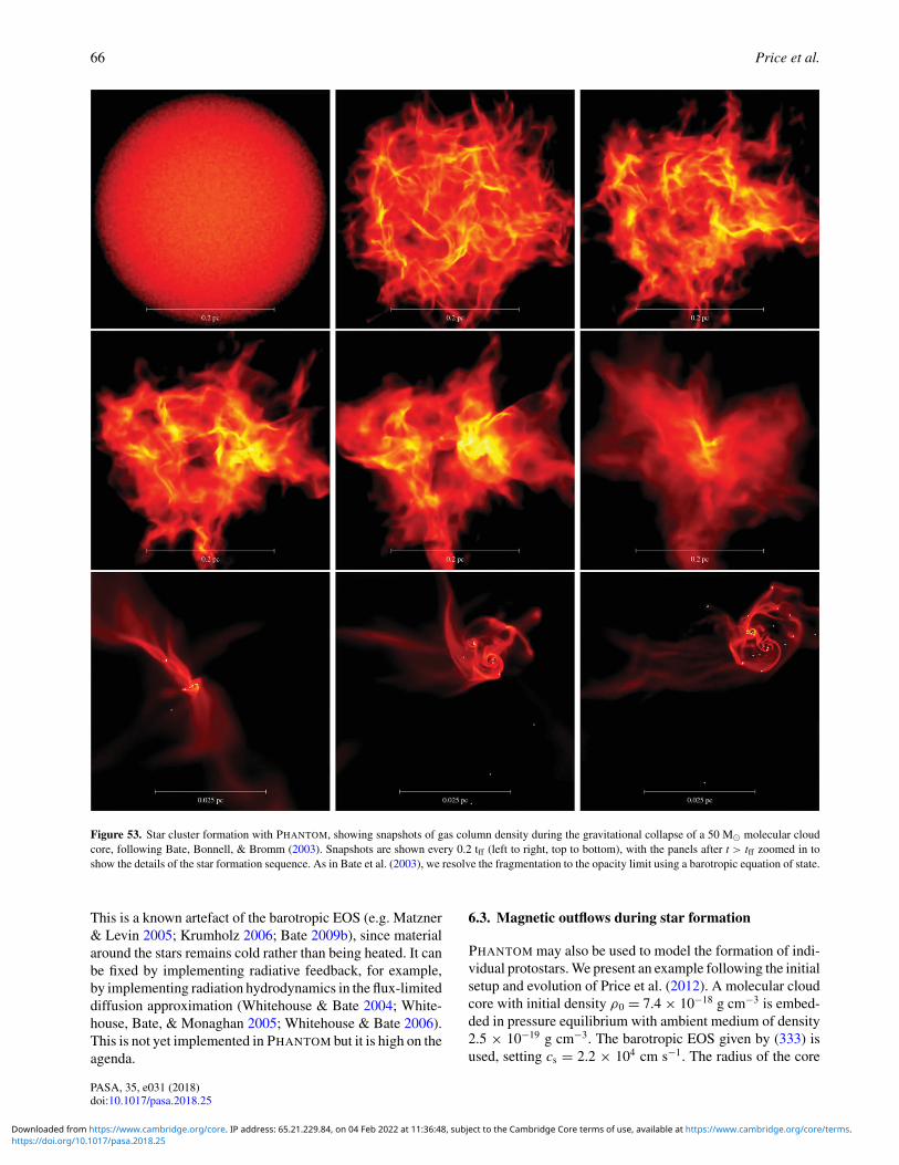
66 Price et al.

Figure 53. Star cluster formation with PHANTOM, showing snapshots of gas column density during the gravitational collapse of a 50 M� molecular cloudcore, following Bate, Bonnell, & Bromm (2003). Snapshots are shown every 0.2 tff (left to right, top to bottom), with the panels after t > tff zoomed in toshow the details of the star formation sequence. As in Bate et al. (2003), we resolve the fragmentation to the opacity limit using a barotropic equation of state.

This is a known artefact of the barotropic EOS (e.g. Matzner& Levin 2005; Krumholz 2006; Bate 2009b), since materialaround the stars remains cold rather than being heated. It canbe fixed by implementing radiative feedback, for example,by implementing radiation hydrodynamics in the flux-limiteddiffusion approximation (Whitehouse & Bate 2004; White-house, Bate, & Monaghan 2005; Whitehouse & Bate 2006).This is not yet implemented in PHANTOM but it is high on theagenda.

6.3. Magnetic outflows during star formation

PHANTOM may also be used to model the formation of indi-vidual protostars. We present an example following the initialsetup and evolution of Price et al. (2012). A molecular cloudcore with initial density ρ0 = 7.4 × 10−18 g cm−3 is embed-ded in pressure equilibrium with ambient medium of density2.5 × 10−19 g cm−3. The barotropic EOS given by (333) isused, setting cs = 2.2 × 104 cm s−1. The radius of the core

PASA, 35, e031 (2018)doi:10.1017/pasa.2018.25






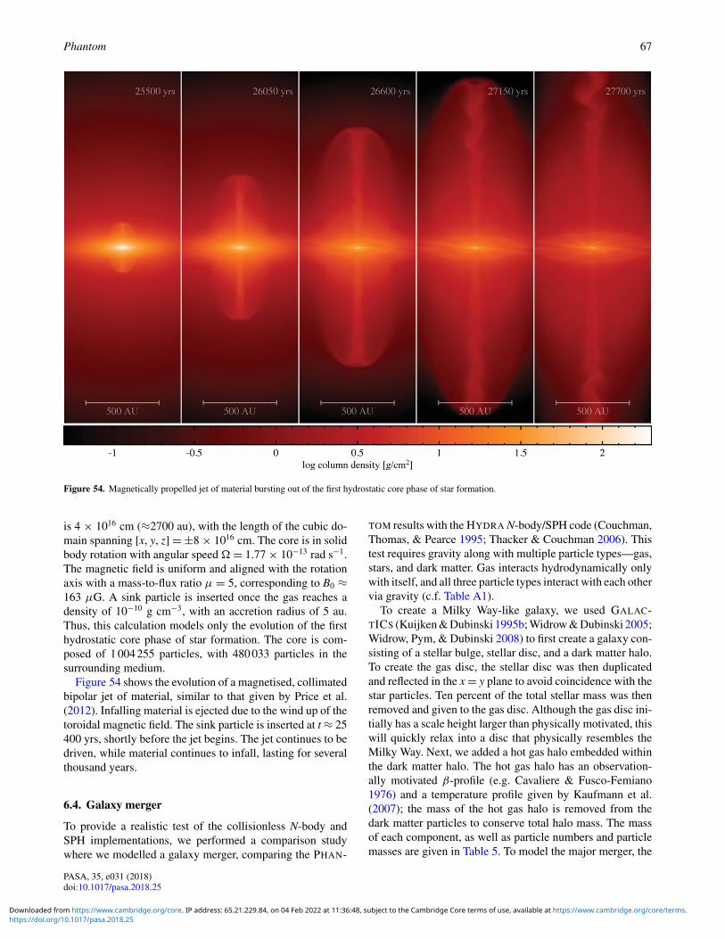
Phantom 67

Figure 54. Magnetically propelled jet of material bursting out of the first hydrostatic core phase of star formation.

is 4 × 1016 cm (≈2700 au), with the length of the cubic do-main spanning [x, y, z] = ±8 × 1016 cm. The core is in solidbody rotation with angular speed � = 1.77 × 10−13 rad s−1.The magnetic field is uniform and aligned with the rotationaxis with a mass-to-flux ratio μ = 5, corresponding to B0 ≈163 μG. A sink particle is inserted once the gas reaches adensity of 10−10 g cm−3, with an accretion radius of 5 au.Thus, this calculation models only the evolution of the firsthydrostatic core phase of star formation. The core is com-posed of 1 004 255 particles, with 480 033 particles in thesurrounding medium.

Figure 54 shows the evolution of a magnetised, collimatedbipolar jet of material, similar to that given by Price et al.(2012). Infalling material is ejected due to the wind up of thetoroidal magnetic field. The sink particle is inserted at t ≈ 25400 yrs, shortly before the jet begins. The jet continues to bedriven, while material continues to infall, lasting for severalthousand years.

6.4. Galaxy merger

To provide a realistic test of the collisionless N-body andSPH implementations, we performed a comparison studywhere we modelled a galaxy merger, comparing the PHAN-

TOM results with the HYDRA N-body/SPH code (Couchman,Thomas, & Pearce 1995; Thacker & Couchman 2006). Thistest requires gravity along with multiple particle types—gas,stars, and dark matter. Gas interacts hydrodynamically onlywith itself, and all three particle types interact with each othervia gravity (c.f. Table A1).

To create a Milky Way-like galaxy, we used GALAC-TICS (Kuijken & Dubinski 1995b; Widrow & Dubinski 2005;Widrow, Pym, & Dubinski 2008) to first create a galaxy con-sisting of a stellar bulge, stellar disc, and a dark matter halo.To create the gas disc, the stellar disc was then duplicatedand reflected in the x = y plane to avoid coincidence with thestar particles. Ten percent of the total stellar mass was thenremoved and given to the gas disc. Although the gas disc ini-tially has a scale height larger than physically motivated, thiswill quickly relax into a disc that physically resembles theMilky Way. Next, we added a hot gas halo embedded withinthe dark matter halo. The hot gas halo has an observation-ally motivated β-profile (e.g. Cavaliere & Fusco-Femiano1976) and a temperature profile given by Kaufmann et al.(2007); the mass of the hot gas halo is removed from thedark matter particles to conserve total halo mass. The massof each component, as well as particle numbers and particlemasses are given in Table 5. To model the major merger, the

PASA, 35, e031 (2018)doi:10.1017/pasa.2018.25






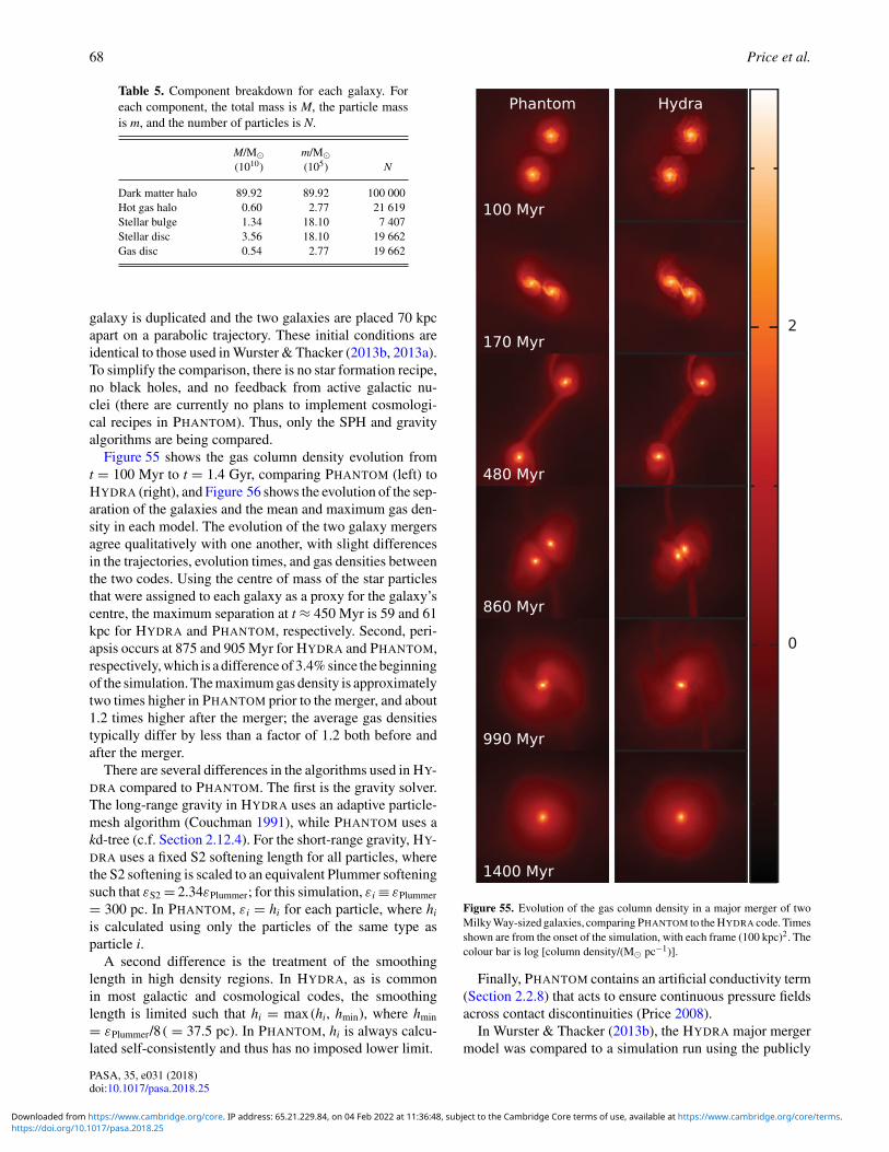
68 Price et al.

Table 5. Component breakdown for each galaxy. Foreach component, the total mass is M, the particle massis m, and the number of particles is N.

M/M� m/M�(1010) (105) N

Dark matter halo 89.92 89.92 100 000Hot gas halo 0.60 2.77 21 619Stellar bulge 1.34 18.10 7 407Stellar disc 3.56 18.10 19 662Gas disc 0.54 2.77 19 662

galaxy is duplicated and the two galaxies are placed 70 kpcapart on a parabolic trajectory. These initial conditions areidentical to those used in Wurster & Thacker (2013b, 2013a).To simplify the comparison, there is no star formation recipe,no black holes, and no feedback from active galactic nu-clei (there are currently no plans to implement cosmologi-cal recipes in PHANTOM). Thus, only the SPH and gravityalgorithms are being compared.

Figure 55 shows the gas column density evolution fromt = 100 Myr to t = 1.4 Gyr, comparing PHANTOM (left) toHYDRA (right), and Figure 56 shows the evolution of the sep-aration of the galaxies and the mean and maximum gas den-sity in each model. The evolution of the two galaxy mergersagree qualitatively with one another, with slight differencesin the trajectories, evolution times, and gas densities betweenthe two codes. Using the centre of mass of the star particlesthat were assigned to each galaxy as a proxy for the galaxy’scentre, the maximum separation at t ≈ 450 Myr is 59 and 61kpc for HYDRA and PHANTOM, respectively. Second, peri-apsis occurs at 875 and 905 Myr for HYDRA and PHANTOM,respectively, which is a difference of 3.4% since the beginningof the simulation. The maximum gas density is approximatelytwo times higher in PHANTOM prior to the merger, and about1.2 times higher after the merger; the average gas densitiestypically differ by less than a factor of 1.2 both before andafter the merger.

There are several differences in the algorithms used in HY-DRA compared to PHANTOM. The first is the gravity solver.The long-range gravity in HYDRA uses an adaptive particle-mesh algorithm (Couchman 1991), while PHANTOM uses akd-tree (c.f. Section 2.12.4). For the short-range gravity, HY-DRA uses a fixed S2 softening length for all particles, wherethe S2 softening is scaled to an equivalent Plummer softeningsuch that εS2 = 2.34εPlummer; for this simulation, εi ≡ εPlummer

= 300 pc. In PHANTOM, εi = hi for each particle, where hi

is calculated using only the particles of the same type asparticle i.

A second difference is the treatment of the smoothinglength in high density regions. In HYDRA, as is commonin most galactic and cosmological codes, the smoothinglength is limited such that hi = max (hi, hmin), where hmin

= εPlummer/8 ( = 37.5 pc). In PHANTOM, hi is always calcu-lated self-consistently and thus has no imposed lower limit.

Figure 55. Evolution of the gas column density in a major merger of twoMilky Way-sized galaxies, comparing PHANTOM to the HYDRA code. Timesshown are from the onset of the simulation, with each frame (100 kpc)2. Thecolour bar is log [column density/(M� pc−1)].

Finally, PHANTOM contains an artificial conductivity term(Section 2.2.8) that acts to ensure continuous pressure fieldsacross contact discontinuities (Price 2008).

In Wurster & Thacker (2013b), the HYDRA major mergermodel was compared to a simulation run using the publicly

PASA, 35, e031 (2018)doi:10.1017/pasa.2018.25






Phantom 69

0

10

20

30

40

50

60

70Se

para

tion

[kpc

]Phantom

Hydra

10-25

10-24

10-23

10-22

10-21

0 200 400 600 800 1000 1200 1400

ρ gas

[g

cm-3

]

Time [Myr]

maximummean

Figure 56. Top: The evolution of the separation of the galaxies, using centreof mass of the star particles that were assigned to each galaxy as a proxyfor the galaxy’s centre; the stars are sufficiently mixed after 1000 Myr,thus a meaningful separation cannot be calculated. Bottom: The evolu-tion of the maximum (solid) and mean (dashed) gas densities for eachmodel.

available version of GADGET2 (Springel et al. 2001; Springel& Hernquist 2002). As here, the comparison was simpli-fied such that only the gravity and SPH solvers were beingcompared. They found that the galaxies in each simulationfollowed similar trajectories and both models reached sec-ond periapsis within 0.2% of one another, as measured fromthe beginning of the simulation. Note that both HYDRA andGADGET2 were both written primarily to solve galactic andcosmological models.

The quantitive difference in results may be attributed to theimproved SPH algorithms in PHANTOM compared to HY-DRA. The higher density in HYDRA is consistent with theresults in Richardson et al. (2016), who found higher den-sities in HYDRA compared to the adaptive mesh refinementcode RAMSES (Teyssier 2002). It was determined that thiswas a result of a combination of the artificial viscosity, hmin

and the suppression of ‘mixing’ (which occurs when no ther-mal conductivity is applied).

6.5. Gap opening in dusty discs

Our final example is taken from Dipierro et al. (2016) andbuilds on our recent studies of dust dynamics in protoplan-etary discs with PHANTOM (e.g. Dipierro et al. 2015; Ra-gusa et al. 2017). We perform calculations using the two-

fluid approach, setting up a disc with 500 000 gas particlesand 100 000 dust particles with �∝r−0.1 between 1 and 120au with a total disc mass of 2 × 10−4 M�. The disc mass ischosen to place the mm dust particles in a regime where theStokes number is greater than unity. The initial dust-to-gasratio is 0.01 and we assume a locally isothermal EOS withcs∝r−0.35, normalised such that H/R = 0.05 at 1 au. We usethe minimum disc viscosity possible, setting αAV = 0.1.

Figure 57 shows the results of two calculations employ-ing planets of mass 0.1 MJupiter (top row) and 1.0 MJupiter

(bottom) embedded in a disc around a 1.3 M� star. Left andright panels show gas and dust surface densities, respectively.While the theory of gap opening in gaseous discs is relativelywell understood as a competition between the gravitationaltorque from the planet trying to open a gap and the viscoustorques trying to close it (e.g. Goldreich & Tremaine 1979,1980), gap opening in dusty discs is less well understood (seee.g. Paardekooper & Mellema 2004, 2006). In Dipierro et al.(2016), we identified two regimes for gap opening in dustydiscs where gap opening in the dust disc is either resistedor assisted by the gas–dust drag. The top row of Figure 57demonstrates that low mass planets can carve a gap whichis visible only in the dust disc, while for high mass plan-ets (bottom row), there is a gap opened in both gas anddust but it is deeper in the dust. Moreover, the gap open-ing mechanism by low mass planets has been further inves-tigated in Dipierro & Laibe (2017). They derived a grainsize-dependent criterion for dust gap opening in discs, anestimate of the location of the outer edge of the dust gapand an estimate of the minimum Stokes number above whichlow-mass planets are able to carve gaps which appear onlyin the dust disc. These predictions has been tested againstPHANTOM simulations of planet–disc interaction in a broadrange of dusty protoplanetary discs, finding a remarkableagreement between the theoretical model and the numericalexperiments.

Interestingly, our prediction of dust gaps that are not coin-cident with gas gaps for low mass planets appears to be ob-served in recent observations of the TW Hya protoplanetarydisc, by comparing VLT-SPHERE imaging of the scatteredlight emission from small dust grains (van Boekel et al. 2017;tracing the gas) to ALMA images of the mm dust emission(Andrews et al. 2016).

7 SUMMARY

We have outlined the algorithms and physics currently im-plemented in the PHANTOM SPH and MHD code in the hopethat this will prove useful to both users and developers ofthe code. We have also demonstrated the performance of thecode as it currently stands on a series of standard test prob-lems, most with known or analytic solutions. While no codeis ever ‘finished’ nor bug free, it is our hope that the codeas it stands will prove useful to the scientific community.Works in progress for future code releases include radiation

PASA, 35, e031 (2018)doi:10.1017/pasa.2018.25






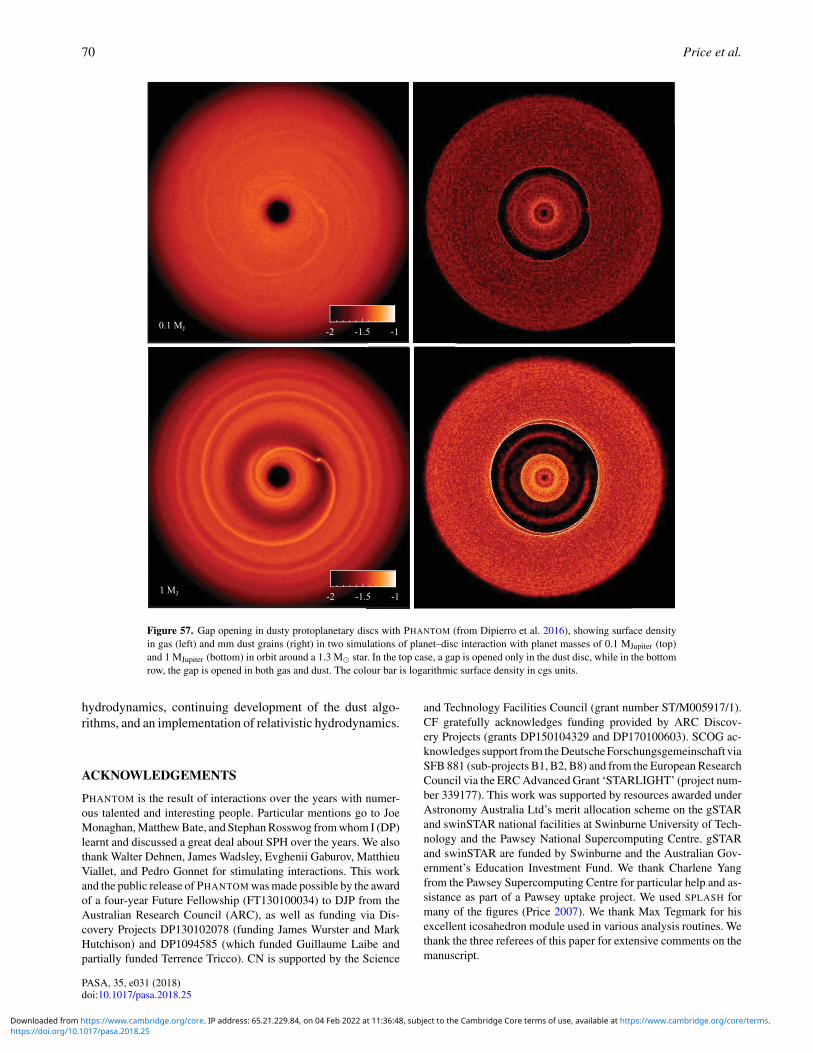
70 Price et al.

-2 -1.5 -10.1 MJ

-2 -1.5 -11 MJ

Figure 57. Gap opening in dusty protoplanetary discs with PHANTOM (from Dipierro et al. 2016), showing surface densityin gas (left) and mm dust grains (right) in two simulations of planet–disc interaction with planet masses of 0.1 MJupiter (top)and 1 MJupiter (bottom) in orbit around a 1.3 M� star. In the top case, a gap is opened only in the dust disc, while in the bottomrow, the gap is opened in both gas and dust. The colour bar is logarithmic surface density in cgs units.

hydrodynamics, continuing development of the dust algo-rithms, and an implementation of relativistic hydrodynamics.

ACKNOWLEDGEMENTS

PHANTOM is the result of interactions over the years with numer-ous talented and interesting people. Particular mentions go to JoeMonaghan, Matthew Bate, and Stephan Rosswog from whom I (DP)learnt and discussed a great deal about SPH over the years. We alsothank Walter Dehnen, James Wadsley, Evghenii Gaburov, MatthieuViallet, and Pedro Gonnet for stimulating interactions. This workand the public release of PHANTOM was made possible by the awardof a four-year Future Fellowship (FT130100034) to DJP from theAustralian Research Council (ARC), as well as funding via Dis-covery Projects DP130102078 (funding James Wurster and MarkHutchison) and DP1094585 (which funded Guillaume Laibe andpartially funded Terrence Tricco). CN is supported by the Science

and Technology Facilities Council (grant number ST/M005917/1).CF gratefully acknowledges funding provided by ARC Discov-ery Projects (grants DP150104329 and DP170100603). SCOG ac-knowledges support from the Deutsche Forschungsgemeinschaft viaSFB 881 (sub-projects B1, B2, B8) and from the European ResearchCouncil via the ERC Advanced Grant ‘STARLIGHT’ (project num-ber 339177). This work was supported by resources awarded underAstronomy Australia Ltd’s merit allocation scheme on the gSTARand swinSTAR national facilities at Swinburne University of Tech-nology and the Pawsey National Supercomputing Centre. gSTARand swinSTAR are funded by Swinburne and the Australian Gov-ernment’s Education Investment Fund. We thank Charlene Yangfrom the Pawsey Supercomputing Centre for particular help and as-sistance as part of a Pawsey uptake project. We used SPLASH formany of the figures (Price 2007). We thank Max Tegmark for hisexcellent icosahedron module used in various analysis routines. Wethank the three referees of this paper for extensive comments on themanuscript.

PASA, 35, e031 (2018)doi:10.1017/pasa.2018.25






Phantom 71

References

Abel, T. 2011, MNRAS, 413, 271Abel, T., Anninos, P., Zhang, Y., & Norman, M. L. 1997, NewA, 2,

181Agertz, O., et al. 2007, MNRAS, 380, 963Alexiades, V., Amiez, G., & Gremaud, P.-A. 1996, CNME, 12, 31Allen, C., & Santillan, A. 1991, RMxAA, 22, 255Andrews, S. M., et al. 2016, ApJ, 820, L40Artymowicz, P., & Lubow, S. H. 1994, ApJ, 421, 651Artymowicz, P., & Lubow, S. H. 1996, ApJ, 467, L77Athanassoula, E., Fady, E., Lambert, J. C., & Bosma, A. 2000, MN-

RAS, 314, 475Bagla, J. S., & Khandai, N. 2009, MNRAS, 396, 2211Ballabio, G., Dipierro, G., Veronesi, B., Lodato, G., Hutchison, M.,

Laibe, G., & Price, D. J. 2018, MNRAS, 477, 2766Balsara, D. S. 1995, JCoPh, 121, 357Balsara, D. S. 1996, ApJ, 465, 775Balsara, D. S. 1998, ApJS, 116, 133Balsara, D. S., & Kim, J. 2004, ApJ, 602, 1079Balsara, D. S., & Spicer, D. 1999, JCoPh, 148, 133Balsara, D. S., Kim, J., Mac Low, M.-M., & Mathews, G. J. 2004,

ApJ, 617, 339Barmin, A., Kulikovskiy, A. G., & Pogorelov, N. V. 1996, JCoPh,

126, 77Barnes, D. J., Kawata, D., & Wu, K. 2012, MNRAS, 420, 3195Bartosch, L. 2001, IJMPC, 12, 851Bate, M. R. 1995, PhD thesis, University of Cambridge, Cambridge,

UKBate, M. R. 2009a, MNRAS, 392, 590Bate, M. R. 2009b, MNRAS, 392, 1363Bate, M. R., & Bonnell, I. A. 1997, MNRAS, 285, 33Bate, M. R., & Burkert, A. 1997, MNRAS, 288, 1060Bate, M. R., Bonnell, I. A., & Price, N. M. 1995, MNRAS, 277, 362Bate, M. R., Bonnell, I. A., & Bromm, V. 2003, MNRAS, 339, 577Bauer, A., & Springel, V. 2012, MNRAS, 423, 2558Beck, A. M., et al. 2016, MNRAS, 455, 2110Begeman, K. G., Broeils, A. H., & Sanders, R. H. 1991, MNRAS,

249, 523Benz, W. 1990, in Proceedings of the NATO Advanced Research

Workshop on The Numerical Modelling of Nonlinear Stellar Pul-sations Problems and Prospects, Held in Les Arcs, France, March20–24, 1986, ed. J. Robert Buchler (Dordrecht and Boston:Kluwer Academic Publishers)

Benz, W., Cameron, A. G. W., Press, W. H., & Bowers, R. L. 1990,ApJ, 348, 647

Bergin, E. A., Hartmann, L. W., Raymond, J. C., & Ballesteros-Paredes J,. 2004, ApJ, 612, 921

Biermann, L. 1950, ZNatA, 5, 65Binney, J., & Tremaine, S. 1987, Galactic Dynamics (Princeton, NJ:

Princeton University Press)Bocquet, S., Saro, A., Dolag, K., & Mohr, J. J. 2016, MNRAS, 456,

2361Boily, C. M., Kroupa, P., & Peñarrubia-Garrido, J. 2001, NewA, 6,

27Bonafede, A., Dolag, K., Stasyszyn, F., Murante, G., & Borgani, S.

2011, MNRAS, 418, 2234Bonet, J., & Lok, T-S. L. 1999, CMAME, 180, 97Bonnell, I. A., Bate, M. R., Clarke, C. J., & Pringle, J. E. 1997,

MNRAS, 285, 201

Bonnerot, C., Rossi, E. M., Lodato, G., & Price, D. J. 2016,MNRAS, 455, 2253

Bonnerot, C., Price, D. J., Lodato, G., & Rossi, E. M. 2017,MNRAS, 469, 4879

Børve, S., Omang, M., & Trulsen, J. 2001, ApJ, 561, 82Børve, S., Omang, M., & Trulsen, J. 2004, ApJS, 153, 447Brio, M., & Wu, C. C. 1988, JCoPh, 75, 400Brookshaw, L. 1985, PASA, 6, 207Brookshaw, L. 1994, MmSAI, 65, 1033Bürzle, F., Clark, P. C., Stasyszyn, F., Greif, T., Dolag, K., Klessen,

R. S., & Nielaba, P. 2011a, MNRAS, 412, 171Bürzle, F., Clark, P. C., Stasyszyn, F., Dolag, K., & Klessen R. S,.

2011b, MNRAS, 417, L61Cabezón, R. M., García-Senz, D., & Relaño, A. 2008, JCoPh, 227,

8523Caldwell, J. A. R., & Ostriker, J. P. 1981, ApJ, 251, 61Cartwright, A., Stamatellos, D., & Whitworth, A. P. 2009, MNRAS,

395, 2373Cavaliere, A., & Fusco-Femiano, R. 1976, A&A, 49, 137Cerioli, A., Lodato, G., & Price, D. J. 2016, MNRAS, 457, 939Cha, S.-H., & Whitworth, A. P. 2003, MNRAS, 340, 73Chabrier, G. 2005, in Astrophysics and Space Science Library, Vol.

327, Proceedings of The Initial Mass Function 50 Years Later,ed. E. Corbelli, F. Palle, & H. Zinnecker (Dordrecht: Springer),41

Chapman, S., & Cowling, T. G. 1970, The Mathematical Theory ofNon-Uniform Gases. An Account of the Kinetic Theory of Vis-cosity, Thermal Conduction and Diffusion in Gases (Cambridge:Cambridge University Press)

Chin, S. A., & Chen, C. R. 2005, CeMDA, 91, 301Choi, E., Kim, J., & Wiita, P. J. 2009, ApJS, 181, 413Chow, E., & Monaghan, J. J. 1997, JCoPh, 134, 296Cossins, P., Lodato, G., & Clarke, C. J. 2009, MNRAS, 393, 1157Couchman, H. M. P. 1991, ApJ, 368, L23Couchman, H. M. P., Thomas, P. A., & Pearce, F. R. 1995, ApJ, 452,

797Coughlin, E. R., & Nixon, C. 2015, ApJ, 808, L11Coughlin, E. R., Armitage, P. J., Nixon, C., & Begelman, M. C.

2017, MNRAS 465, 3840Coughlin, E. R., Nixon, C., Begelman, M. C., & Armitage, P. J.

2016b, MNRAS, 459, 3089Courant, R., Friedrichs, K., & Lewy, H. 1928, MatAn, 100, 32Cox, D. P., & Gómez, G. C. 2002, ApJS, 142, 261Cullen, L., & Dehnen, W. 2010, MNRAS, 408, 669Cummins, S. J., & Rudman, M. 1999, JCoPh, 152, 584Dahlburg, R. B., & Picone, J. M. 1989, PhFlB, 1, 2153Dai, W., & Woodward, P. R. 1994a, JCoPh, 111, 354Dai, W., & Woodward, P. R. 1994b, JCoPh, 115, 485Dai, W., & Woodward, P. R. 1998, ApJ, 494, 317de Val-Borro, M., et al. 2006, MNRAS, 370, 529Dedner, A., Kemm, F., Kröner, D., Munz, C.-D., Schnitzer, T., &

Wesenberg, M. 2002, JCoPh, 175, 645Dehnen, W. 2000a, AJ, 119, 800Dehnen, W. 2000b, ApJ, 536, L39Dehnen, W. 2001, MNRAS, 324, 273Dehnen, W., & Aly, H. 2012, MNRAS, 425, 1068Dehnen, W., & Read, J. I. 2011, EPJP, 126, 55Diehl, S., Rockefeller, G., Fryer, C. L., Riethmiller, D., & Statler T.

S,. 2015, PASA, 32, 48Dipierro, G., & Laibe, G. 2017, MNRAS, 469, 1932

PASA, 35, e031 (2018)doi:10.1017/pasa.2018.25


https://doi.org/10.1111/j.1365-2966.2010.18133.x

http://adsabs.harvard.edu/abs/2011MNRAS.413..271A


https://doi.org/10.1016/S1384-1076(97)00010-9

http://adsabs.harvard.edu/abs/1997NewA....2..181A

http://adsabs.harvard.edu/abs/1997NewA....2..181A

https://doi.org/10.1111/j.1365-2966.2007.12183.x



https://doi.org/10.1002/(SICI)1099-0887(199601)12:1<31::AID-CNM950&

http://adsabs.harvard.edu/abs/1991RMxAA..22..255A

http://adsabs.harvard.edu/abs/1991RMxAA..22..255A

https://doi.org/10.3847/2041-8205/820/2/L40

http://adsabs.harvard.edu/abs/2016ApJ...820L..40A


https://doi.org/10.1086/173679

http://adsabs.harvard.edu/abs/1994ApJ...421..651A

http://adsabs.harvard.edu/abs/1994ApJ...421..651A

https://doi.org/10.1086/310200



https://doi.org/10.1046/j.1365-8711.2000.03316.x



https://doi.org/10.1111/j.1365-2966.2009.14880.x

http://adsabs.harvard.edu/abs/2009MNRAS.396.2211B


https://doi.org/10.1093/mnras/sty642



https://doi.org/10.1016/S0021-9991(95)90221-X

http://adsabs.harvard.edu/abs/1995JCoPh.121..357B


https://doi.org/10.1086/177462

http://adsabs.harvard.edu/abs/1996ApJ...465..775B


https://doi.org/10.1086/313093

http://adsabs.harvard.edu/abs/1998ApJS..116..133B


https://doi.org/10.1086/381051

http://adsabs.harvard.edu/abs/2004ApJ...602.1079B

http://adsabs.harvard.edu/abs/2004ApJ...602.1079B

https://doi.org/10.1006/jcph.1998.6108



https://doi.org/10.1086/425297




http://adsabs.harvard.edu/abs/1996JCoPh.126...77B

http://adsabs.harvard.edu/abs/1996JCoPh.126...77B

https://doi.org/10.1111/j.1365-2966.2011.20247.x



https://doi.org/10.1142/S0129183101002012

http://adsabs.harvard.edu/abs/2001IJMPC..12..851B

http://adsabs.harvard.edu/abs/2001IJMPC..12..851B

https://doi.org/10.1111/j.1365-2966.2008.14106.x

http://adsabs.harvard.edu/abs/2009MNRAS.392..590B


https://doi.org/10.1111/j.1365-2966.2008.14165.x



http://adsabs.harvard.edu/abs/1997MNRAS.285...33B

http://adsabs.harvard.edu/abs/1997MNRAS.285...33B





https://doi.org/10.1046/j.1365-8711.2003.06210.x



https://doi.org/10.1111/j.1365-2966.2012.21058.x



https://doi.org/10.1093/mnras/stv2443





https://doi.org/10.1086/168273



https://doi.org/10.1086/422578



http://adsabs.harvard.edu/abs/1950ZNatA...5...65B

http://adsabs.harvard.edu/abs/1950ZNatA...5...65B




https://doi.org/10.1016/S1384-1076(01)00039-2

http://adsabs.harvard.edu/abs/2001NewA....6...27B

http://adsabs.harvard.edu/abs/2001NewA....6...27B

https://doi.org/10.1111/j.1365-2966.2011.19523.x








https://doi.org/10.1093/mnras/stx1210



https://doi.org/10.1086/323228

http://adsabs.harvard.edu/abs/2001ApJ...561...82B

http://adsabs.harvard.edu/abs/2001ApJ...561...82B

https://doi.org/10.1086/421520



https://doi.org/10.1016/0021-9991(88)90120-9

http://adsabs.harvard.edu/abs/1988JCoPh..75..400B

http://adsabs.harvard.edu/abs/1988JCoPh..75..400B

http://adsabs.harvard.edu/abs/1985PASAu...6..207B

http://adsabs.harvard.edu/abs/1985PASAu...6..207B

http://adsabs.harvard.edu/abs/1994MmSAI..65.1033B

http://adsabs.harvard.edu/abs/1994MmSAI..65.1033B

https://doi.org/10.1111/j.1365-2966.2010.17896.x



https://doi.org/10.1111/j.1745-3933.2011.01120.x

http://adsabs.harvard.edu/abs/2011MNRAS.417L..61B

http://adsabs.harvard.edu/abs/2011MNRAS.417L..61B

https://doi.org/10.1016/j.jcp.2008.06.014

http://adsabs.harvard.edu/abs/2008JCoPh.227.8523C

http://adsabs.harvard.edu/abs/2008JCoPh.227.8523C

https://doi.org/10.1086/159441

http://adsabs.harvard.edu/abs/1981ApJ...251...61C

http://adsabs.harvard.edu/abs/1981ApJ...251...61C

https://doi.org/10.1111/j.1365-2966.2009.14720.x

http://adsabs.harvard.edu/abs/2009MNRAS.395.2373C


http://adsabs.harvard.edu/abs/1976A&A...49..137C

http://adsabs.harvard.edu/abs/1976A&A...49..137C

https://doi.org/10.1093/mnras/stw034

http://adsabs.harvard.edu/abs/2016MNRAS.457..939C


https://doi.org/10.1046/j.1365-8711.2003.06266.x

http://adsabs.harvard.edu/abs/2003MNRAS.340...73C

http://adsabs.harvard.edu/abs/2003MNRAS.340...73C

https://doi.org/10.1007/s10569-004-4622-z

http://adsabs.harvard.edu/abs/2005CeMDA..91..301C

http://adsabs.harvard.edu/abs/2005CeMDA..91..301C

https://doi.org/10.1088/0067-0049/181/2/413

http://adsabs.harvard.edu/abs/2009ApJS..181..413C



http://adsabs.harvard.edu/abs/1997JCoPh.134..296C


https://doi.org/10.1111/j.1365-2966.2008.14275.x



https://doi.org/10.1086/185939

http://adsabs.harvard.edu/abs/1991ApJ...368L..23C


https://doi.org/10.1086/176348

http://adsabs.harvard.edu/abs/1995ApJ...452..797C

http://adsabs.harvard.edu/abs/1995ApJ...452..797C

https://doi.org/10.1088/2041-8205/808/1/L11




http://adsabs.harvard.edu/abs/2017MNRAS.465.3840

http://adsabs.harvard.edu/abs/2017MNRAS.465.3840




https://doi.org/10.1007/BF01448839

http://adsabs.harvard.edu/abs/1928MatAn.100...32C

http://adsabs.harvard.edu/abs/1928MatAn.100...32C

https://doi.org/10.1086/341946



https://doi.org/10.1111/j.1365-2966.2010.17158.x






https://doi.org/10.1063/1.859081

http://adsabs.harvard.edu/abs/1989PhFlB...1.2153D

http://adsabs.harvard.edu/abs/1989PhFlB...1.2153D


http://adsabs.harvard.edu/abs/1994JCoPh.111..354D





https://doi.org/10.1086/305176

http://adsabs.harvard.edu/abs/1998ApJ...494..317D


https://doi.org/10.1111/j.1365-2966.2006.10488.x

http://adsabs.harvard.edu/abs/2006MNRAS.370..529D





https://doi.org/10.1086/301226

http://adsabs.harvard.edu/abs/2000AJ....119..800D

http://adsabs.harvard.edu/abs/2000AJ....119..800D

https://doi.org/10.1086/312724

http://adsabs.harvard.edu/abs/2000ApJ...536L..39D

http://adsabs.harvard.edu/abs/2000ApJ...536L..39D

https://doi.org/10.1046/j.1365-8711.2001.04237.x



https://doi.org/10.1111/j.1365-2966.2012.21439.x

http://adsabs.harvard.edu/abs/2012MNRAS.425.1068D


https://doi.org/10.1140/epjp/i2011-11055-3

http://adsabs.harvard.edu/abs/2011EPJP..126...55D

http://adsabs.harvard.edu/abs/2011EPJP..126...55D


http://adsabs.harvard.edu/abs/2015PASA...32...48D

http://adsabs.harvard.edu/abs/2015PASA...32...48D








72 Price et al.

Dipierro, G., Price, D., Laibe, G., Hirsh, K., Cerioli, A., & LodatoG,. 2015, MNRAS, 453, L73

Dipierro, G., Laibe, G., Price, D. J., & Lodato, G. 2016, MNRAS,459, L1

Dobbs, C. L., Glover, S. C. O., Clark, P. C., & Klessen, R. S. 2008,MNRAS, 389, 1097

Dobbs, C. L., Price, D. J., Pettitt, A. R., Bate, M. R., & Tricco T. S,.2016, MNRAS, 461, 4482

Dolag, K., & Stasyszyn, F. 2009, MNRAS, 398, 1678Dolag, K., Vazza, F., Brunetti, G., & Tormen, G. 2005, MNRAS,

364, 753Dopcke, G., Glover, S. C. O., Clark, P. C., & Klessen, R. S. 2011,

ApJ, 729, L3Dogan, S., Nixon, C., King, A., & Price, D. J. 2015, MNRAS, 449,

1251Draine, B. T., & Bertoldi, F. 1996, ApJ, 468, 269Epstein, P. S. 1924, PhRv, 23, 710Escala, A., Larson, R. B., Coppi, P. S., & Mardones, D. 2004, ApJ,

607, 765Español, P., & Revenga, M. 2003, PhRvE, 67, 026705Eswaran, V., & Pope, S. B. 1988, CF, 16, 257Evrard, A. E. 1988, MNRAS, 235, 911Facchini, S., Lodato, G., & Price, D. J. 2013, MNRAS, 433,

2142Falle, S. A. E. G. 2003, MNRAS, 344, 1210Falle, S. A. E. G., & Komissarov, S. S. 2001, JPlPh, 65, 29Fan, L.-S., & Zhu, C. 1998, Principles of Gas-Solid Flows (Cam-

bridge: Cambridge University Press)Farr, W. M., & Bertschinger, E. 2007, ApJ, 663, 1420Fassio, F., & Probstein, R. F. 1970, AIAAJ, 8, 772Federrath, C., Klessen, R. S., & Schmidt, W. 2008, ApJ, 688, L79Federrath, C., Roman-Duval, J., Klessen, R. S., Schmidt, W., & Mac

Low M.-M,. 2010a, A&A, 512, A81Federrath, C., Banerjee, R., Clark, P. C., & Klessen, R. S. 2010b,

ApJ, 713, 269Feng, H. Q., Lin, C. C., Chao, J. K., Wu, D. J., Lyu, L. H., & Lee

L.-C,. 2007, JGRA, 112, 10104Ferland, G. J., Peterson, B. M., Horne, K., Welsh, W. F., & Nahar

S. N,. 1992, ApJ, 387, 95Flebbe, O., Muenzel, S., Herold, H., Riffert, H., & Ruder, H. 1994,

ApJ, 431, 754Forgan, D., Price, D. J., & Bonnell, I. 2017, MNRAS, 466, 3406Fryer, C. L., Hungerford, A. L., & Rockefeller, G. 2007, IJMPAD,

16, 941Fulk, D. A., & Quinn, D. W. 1996, JCoPh, 126, 165Furth, H. P., Killeen, J., & Rosenbluth, M. N. 1963, PhFl, 6, 459Gafton, E., & Rosswog, S. 2011, MNRAS, 418, 770Gammie, C. F. 2001, ApJ, 553, 174García-Senz, D., Cabezón, R. M., Escartín, J. A., Ebinger, K. 2014,

A&A, 570, A14Gardiner, T. A., & Stone, J. M. 2005, JCoPh, 205, 509Gardiner, T. A., & Stone, J. M. 2008, JCoPh, 227, 4123Gingold, R. A., & Monaghan, J. J. 1977, MNRAS, 181, 375Gingold, R. A., & Monaghan, J. J. 1978, MNRAS, 184, 481Gingold, R. A., & Monaghan, J. J. 1980, MNRAS, 191, 897Gingold, R. A., & Monaghan, J. J. 1982a, PASA, 4, 378Gingold, R. A., & Monaghan, J. J. 1982b, JCoPh, 46, 429Gingold, R. A., & Monaghan, J. J. 1983, MNRAS, 204, 715Glover, S. C. O., & Clark, P. C. 2012, MNRAS, 421, 116Glover, S. C. O., & Jappsen, A.-K. 2007, ApJ, 666, 1Glover, S. C. O., & Mac Low, M.-M. 2007, ApJS, 169, 239

Glover, S. C. O., Federrath, C., Mac Low, M.-M., & Klessen, R. S.2010, MNRAS, 404, 2

Goffrey, et al. 2017, A&A 600, A7Goldreich, P., & Tremaine, S. 1979, ApJ, 233, 857Goldreich, P., & Tremaine, S. 1980, ApJ, 241, 425Goldsmith, P. F., & Langer, W. D. 1978, ApJ, 222, 881Gray, J., Monaghan, J. J., & Swift, R. P. 2001, CMAME, 190, 6641Graziani, C., Tzeferacos, P., Lee, D., Lamb, D. Q., Weide, K.,

Fatenejad, M., & Miller, J. 2015, ApJ, 802, 43Hairer, E., Lubich, C., & Wanner, G. 2003, AcNum, 12, 399Haworth, T. J., et al. 2016, PASA, 33, e053Herant, M. 1994, MmSAI, 65, 1013Hernquist, L. 1990, ApJ, 356, 359Hernquist, L., & Barnes, J. E. 1990, ApJ, 349, 562Hernquist, L., & Katz, N. 1989, ApJS, 70, 419Hollenbach, D., & McKee, C. F. 1989, ApJ, 342, 306Hopkins, P. F., & Raives, M. J. 2016, MNRAS, 455, 51Hosking, J. G., & Whitworth, A. P. 2004, MNRAS, 347, 994Hu, X. Y., & Adams, N. A. 2006, PhFl, 18, 101702Hu, C.-Y., Naab, T., Walch, S., Moster, B. P., & Oser, L. 2014,

MNRAS, 443, 1173Hubber, D. A., Batty, C. P., McLeod, A., & Whitworth, A. P. 2011,

A&A, 529, A27Hubber, D. A., Allison, R. J., Smith, R., & Goodwin, S. P. 2013a,

MNRAS, 430, 1599Hubber, D. A., Walch, S., & Whitworth, A. P. 2013b, MNRAS, 430,

3261Hubber, D. A., Falle, S. A. E. G., & Goodwin, S. P. 2013c, MNRAS,

432, 711Hubble, E. P. 1930, ApJ, 71, 231Hut, P., Makino, J., & McMillan, S. 1995, ApJ, 443, L93Hutchison, M. A., Price, D. J., Laibe, G., & Maddison, S. T. 2016,

MNRAS, 461, 742Iaconi, R., Reichardt, T., Staff, J., De Marco, O., Passy, J.-C., Price,

D., Wurster, J., & Herwig, F. 2017, MNRAS, 464, 4028Iannuzzi, F., & Dolag, K. 2011, MNRAS, 417, 2846Inutsuka, S.-I. 2002, JCoPh, 179, 238Iwasaki, K. 2015, JCoPh, 302, 359Jubelgas, M., Springel, V., & Dolag, K. 2004, MNRAS, 351,

423Kaufmann, T., Mayer, L., Wadsley, J., Stadel, J., & Moore, B. 2007,

MNRAS, 375, 53Khomenko, E., Vitas, N., Collados, M., & de Vicente, A. 2017,

A&A, 604, A66Khoperskov, S. A., Vasiliev, E. O., Sobolev, A. M., & Khoperskov,

A. V. 2013, MNRAS, 428, 2311Kim, J., Balsara, D., & Mac Low, M.-M. 2001, JKAS, 34, 333Kitsionas, S., et al. 2009, A&A, 508, 541Krumholz, M. R. 2006, ApJ, 641, L45Kuijken, K., & Dubinski, J. 1995a, MNRAS, 277, 1341Kuijken, K., & Dubinski, J. 1995b, MNRAS, 277, 1341Kwok, S. 1975, ApJ, 198, 583Laibe, G., & Price, D. J. 2011, MNRAS, 418, 1491Laibe, G., & Price, D. J. 2012a, MNRAS, 420, 2345Laibe, G., & Price, D. J. 2012b, MNRAS, 420, 2365Laibe, G., & Price, D. J. 2014a, MNRAS, 440, 2136Laibe, G., & Price, D. J. 2014b, MNRAS, 440, 2147Laibe, G., & Price, D. J. 2014c, MNRAS, 444, 1940Larson, R. B. 1981, MNRAS, 194, 809Lattanzio, J., Monaghan, J., Pongracic, H., & Schwarz, M. 1986,

SIAM JSSC, 7, 591

PASA, 35, e031 (2018)doi:10.1017/pasa.2018.25


https://doi.org/10.1093/mnrasl/slv105

http://adsabs.harvard.edu/abs/2015MNRAS.453L..73D

http://adsabs.harvard.edu/abs/2015MNRAS.453L..73D

https://doi.org/10.1093/mnrasl/slw032

http://adsabs.harvard.edu/abs/2016MNRAS.459L...1D

http://adsabs.harvard.edu/abs/2016MNRAS.459L...1D

https://doi.org/10.1111/j.1365-2966.2008.13646.x






https://doi.org/10.1111/j.1365-2966.2009.15181.x



https://doi.org/10.1111/j.1365-2966.2005.09630.x



https://doi.org/10.1088/2041-8205/729/1/L3

http://adsabs.harvard.edu/abs/2011ApJ...729L...3D

http://adsabs.harvard.edu/abs/2011ApJ...729L...3D




https://doi.org/10.1086/177689



https://doi.org/10.1103/PhysRev.23.710

http://adsabs.harvard.edu/abs/1924PhRv...23..710E

http://adsabs.harvard.edu/abs/1924PhRv...23..710E

https://doi.org/10.1086/386278

http://adsabs.harvard.edu/abs/2004ApJ...607..765E

http://adsabs.harvard.edu/abs/2004ApJ...607..765E

https://doi.org/10.1103/PhysRevE.67.026705

http://adsabs.harvard.edu/abs/2003PhRvE..67b6705E

http://adsabs.harvard.edu/abs/2003PhRvE..67b6705E

http://adsabs.harvard.edu/abs/1988CF.....16..257E

http://adsabs.harvard.edu/abs/1988CF.....16..257E

http://adsabs.harvard.edu/abs/1988MNRAS.235..911E

http://adsabs.harvard.edu/abs/1988MNRAS.235..911E

https://doi.org/10.1093/mnras/stt877

http://adsabs.harvard.edu/abs/2013MNRAS.433.2142F


https://doi.org/10.1046/j.1365-8711.2003.06908.x



https://doi.org/10.1017/S0022377801008856

http://adsabs.harvard.edu/abs/2001JPlPh..65...29F

http://adsabs.harvard.edu/abs/2001JPlPh..65...29F

https://doi.org/10.1086/518641

http://adsabs.harvard.edu/abs/2007ApJ...663.1420F

http://adsabs.harvard.edu/abs/2007ApJ...663.1420F

https://doi.org/10.2514/3.5755

http://adsabs.harvard.edu/abs/1970AIAAJ...8..772F

http://adsabs.harvard.edu/abs/1970AIAAJ...8..772F

https://doi.org/10.1086/595280

http://adsabs.harvard.edu/abs/2008ApJ...688L..79F

http://adsabs.harvard.edu/abs/2008ApJ...688L..79F

https://doi.org/10.1051/0004-6361/200912437

http://adsabs.harvard.edu/abs/2010A&A...512A..81F

http://adsabs.harvard.edu/abs/2010A&A...512A..81F

https://doi.org/10.1088/0004-637X/713/1/269

http://adsabs.harvard.edu/abs/2010ApJ...713..269F


https://doi.org/10.1029/2007JA012311

http://adsabs.harvard.edu/abs/2007JGRA..11210104F

http://adsabs.harvard.edu/abs/2007JGRA..11210104F

https://doi.org/10.1086/171063

http://adsabs.harvard.edu/abs/1992ApJ...387...95F

http://adsabs.harvard.edu/abs/1992ApJ...387...95F

https://doi.org/10.1086/174526






https://doi.org/10.1142/S0218271807010523

http://adsabs.harvard.edu/abs/2007IJMPD..16..941F

http://adsabs.harvard.edu/abs/2007IJMPD..16..941F

http://adsabs.harvard.edu/abs/article/B6WHY-45MGW7K-4D/2/32bb5469dfc6716396e9a54bab0e48a3

http://adsabs.harvard.edu/abs/article/B6WHY-45MGW7K-4D/2/32bb5469dfc6716396e9a54bab0e48a3

https://doi.org/10.1063/1.1706761

http://adsabs.harvard.edu/abs/1963PhFl....6..459F

http://adsabs.harvard.edu/abs/1963PhFl....6..459F

https://doi.org/10.1111/j.1365-2966.2011.19528.x

http://adsabs.harvard.edu/abs/2011MNRAS.418..770G


https://doi.org/10.1086/320631

http://adsabs.harvard.edu/abs/2001ApJ...553..174G


https://doi.org/10.1051/0004-6361/201424260

http://adsabs.harvard.edu/abs/2014A&A...570A..14G

http://adsabs.harvard.edu/abs/2014A&A...570A..14G


http://adsabs.harvard.edu/abs/2005JCoPh.205..509G

http://adsabs.harvard.edu/abs/2005JCoPh.205..509G


http://adsabs.harvard.edu/abs/2008JCoPh.227.4123G

http://adsabs.harvard.edu/abs/2008JCoPh.227.4123G







http://adsabs.harvard.edu/abs/1982PASAu...4..378G

http://adsabs.harvard.edu/abs/1982PASAu...4..378G

https://doi.org/10.1016/0021-9991(82)90025-0

http://adsabs.harvard.edu/abs/1982JCoPh..46..429G

http://adsabs.harvard.edu/abs/1982JCoPh..46..429G



https://doi.org/10.1111/j.1365-2966.2011.20260.x



https://doi.org/10.1086/519445

http://adsabs.harvard.edu/abs/2007ApJ...666....1G

http://adsabs.harvard.edu/abs/2007ApJ...666....1G

https://doi.org/10.1086/512238

http://adsabs.harvard.edu/abs/2007ApJS..169..239G

http://adsabs.harvard.edu/abs/2007ApJS..169..239G

https://doi.org/10.1111/j.1365-2966.2009.15718.x

http://adsabs.harvard.edu/abs/2010MNRAS.404....2G

http://adsabs.harvard.edu/abs/2010MNRAS.404....2G

https://doi.org/10.1051/0004-6361/201628960

http://adsabs.harvard.edu/abs/2016arXiv161010053G

http://adsabs.harvard.edu/abs/2016arXiv161010053G

https://doi.org/10.1086/157448



https://doi.org/10.1086/158356



https://doi.org/10.1086/156206



https://doi.org/10.1088/0004-637X/802/1/43

http://adsabs.harvard.edu/abs/2015ApJ...802...43G

http://adsabs.harvard.edu/abs/2015ApJ...802...43G

https://doi.org/10.1017/S0962492902000144


http://adsabs.harvard.edu/abs/2016PASA...33...53H

http://adsabs.harvard.edu/abs/2016PASA...33...53H

http://adsabs.harvard.edu/abs/1994MmSAI..65.1013H

http://adsabs.harvard.edu/abs/1994MmSAI..65.1013H

https://doi.org/10.1086/168845

http://adsabs.harvard.edu/abs/1990ApJ...356..359H


https://doi.org/10.1086/168343



https://doi.org/10.1086/191344

http://adsabs.harvard.edu/abs/1989ApJS...70..419H

http://adsabs.harvard.edu/abs/1989ApJS...70..419H

https://doi.org/10.1086/167595




http://adsabs.harvard.edu/abs/2016MNRAS.455...51H

http://adsabs.harvard.edu/abs/2016MNRAS.455...51H

https://doi.org/10.1111/j.1365-2966.2004.07273.x

http://adsabs.harvard.edu/abs/2004MNRAS.347..994H


https://doi.org/10.1063/1.2359741

http://adsabs.harvard.edu/abs/2006PhFl...18j1702H

http://adsabs.harvard.edu/abs/2006PhFl...18j1702H

https://doi.org/10.1093/mnras/stu1187

http://adsabs.harvard.edu/abs/2014MNRAS.443.1173H


https://doi.org/10.1051/0004-6361/201014949

http://adsabs.harvard.edu/abs/2011A&A...529A..27H

http://adsabs.harvard.edu/abs/2011A&A...529A..27H

https://doi.org/10.1093/mnras/sts694









https://doi.org/10.1086/143250

http://adsabs.harvard.edu/abs/1930ApJ....71..231H

http://adsabs.harvard.edu/abs/1930ApJ....71..231H

https://doi.org/10.1086/187844

http://adsabs.harvard.edu/abs/1995ApJ...443L..93H

http://adsabs.harvard.edu/abs/1995ApJ...443L..93H





http://adsabs.harvard.edu/abs/2017MNRAS.464.4028I


https://doi.org/10.1111/j.1365-2966.2011.19446.x




http://adsabs.harvard.edu/abs/2002JCoPh.179..238I





https://doi.org/10.1111/j.1365-2966.2004.07801.x

http://adsabs.harvard.edu/abs/2004MNRAS.351..423J

http://adsabs.harvard.edu/abs/2004MNRAS.351..423J

https://doi.org/10.1111/j.1365-2966.2006.11314.x

http://adsabs.harvard.edu/abs/2007MNRAS.375...53K

http://adsabs.harvard.edu/abs/2007MNRAS.375...53K

https://doi.org/10.1051/0004-6361/201630291

http://adsabs.harvard.edu/abs/2017A&A...604A..66K

http://adsabs.harvard.edu/abs/2017A&A...604A..66K

https://doi.org/10.1093/mnras/sts195

http://adsabs.harvard.edu/abs/2013MNRAS.428.2311K


https://doi.org/10.5303/JKAS.2001.34.4.333

http://adsabs.harvard.edu/abs/2001JKAS...34..333K

http://adsabs.harvard.edu/abs/2001JKAS...34..333K

https://doi.org/10.1051/0004-6361/200811170

http://adsabs.harvard.edu/abs/2009A&A...508..541K

http://adsabs.harvard.edu/abs/2009A&A...508..541K

https://doi.org/10.1086/503771

http://adsabs.harvard.edu/abs/2006ApJ...641L..45K

http://adsabs.harvard.edu/abs/2006ApJ...641L..45K





https://doi.org/10.1086/153637

http://adsabs.harvard.edu/abs/1975ApJ...198..583K

http://adsabs.harvard.edu/abs/1975ApJ...198..583K

https://doi.org/10.1111/j.1365-2966.2011.19291.x

http://adsabs.harvard.edu/abs/2011MNRAS.418.1491L


https://doi.org/10.1111/j.1365-2966.2011.20202.x



https://doi.org/10.1111/j.1365-2966.2011.20201.x












http://adsabs.harvard.edu/abs/1981MNRAS.194..809L


https://doi.org/10.1137/0907039





Phantom 73

Le Bourlot, J., Pineau des Forêts, G., & Flower, D. R. 1999, MN-RAS, 305, 802

Lecoanet, D., et al. 2016, MNRAS, 455, 4274Lense, J., & Thirring, H. 1918, PhyZ, 19, 156Lewis, B. T., Bate, M. R., & Price, D. J. 2015, MNRAS, 451,

288Liptai, D., Price, D. J., Wurster, J., & Bate, M. R. 2017, MNRAS,

465, 105Lodato, G., & Price, D. J. 2010, MNRAS, 405, 1212Lodato, G., & Pringle, J. E. 2007, MNRAS, 381, 1287Lodato, G., & Rice, W. K. M. 2004, MNRAS, 351, 630Lodato, G., Nayakshin, S., King, A. R., & Pringle, J. E. 2009, MN-

RAS, 398, 1392Lombardi, J. C., Sills, A., Rasio, F. A., & Shapiro, S. L. 1999,

JCoPh, 152, 687Londrillo, P., & Del Zanna, L. 2000, ApJ, 530, 508Long, K., & Murali, C. 1992, ApJ, 397, 44Lorén-Aguilar, P., & Bate, M. R. 2014, MNRAS, 443, 927Low, C., & Lynden-Bell, D. 1976, MNRAS, 176, 367Lubow, S. H., & Ogilvie, G. I. 2000, ApJ, 538, 326Lubow, S. H., Ogilvie, G. I., & Pringle, J. E. 2002, MNRAS, 337,

706Lucy, L. B. 1977, AJ, 82, 1013Lynden-Bell, D., & Pringle, J. E. 1974, MNRAS, 168, 603Mac Low, M.-M., Balsara, D. S., Kim, J., & de Avillez, M. A. 2005,

ApJ, 626, 864Maddison, S. T. 1998, PhD thesis, Department of Mathematics,

Monash UniversityMaddison, S. T., Murray, J. R., & Monaghan, J. J. 1996, PASA, 13,

66Makino, J., & Aarseth, S. J. 1992, PASJ, 44, 141Makino, J., Hut, P., Kaplan, M., & Saygın, H. 2006, NewA, 12, 124Martin, R. G., Nixon, C., Armitage, P. J., Lubow, S. H., & Price D.

J,. 2014a, ApJ, 790, L34Martin, R. G., Nixon, C., Lubow, S. H., Armitage, P. J., Price, D. J.,

Dogan, S., & King, A. 2014b, ApJ, 792, L33Martos, M., Hernandez, X., Yáñez, M., Moreno, E., & Pichardo B,.

2004, MNRAS, 350, L47Matzner, C. D., & Levin, Y. 2005, ApJ, 628, 817McMillan, P. J., & Dehnen, W. 2007, MNRAS, 378, 541McNally, C. P., Lyra, W., & Passy, J.-C. 2012, ApJS, 201, 18Merritt, D. 1996, AJ, 111, 2462Meru, F., & Bate, M. R. 2011, MNRAS, 411, L1Meru, F., & Bate, M. R. 2012, MNRAS, 427, 2022Miller, M. C., & Lamb, F. K. 1993, ApJ, 413, L43Miniati, F. 2010, JCoPh, 229, 3916Miura, H., & Glass, I. I. 1982, RSPSA, 382, 373Miyamoto, M., & Nagai, R. 1975, PASJ, 27, 533Monaghan, J. J. 1989, JCoPh, 82, 1Monaghan, J. J. 1992, ARA&A, 30, 543Monaghan, J. J. 1997, JCoPh, 136, 298Monaghan, J. J. 2000, JCoPh, 159, 290Monaghan, J. J. 2002, MNRAS, 335, 843Monaghan, J. J. 2005, RPPh, 68, 1703Monaghan, J. J. 2012, AnRFM, 44, 323Monaghan, J. J., & Kocharyan, A. 1995, CoPhC, 87, 225Monaghan, J. J., & Lattanzio, J. C. 1985, A&A, 149, 135Monaghan, J. J., & Lattanzio, J. C. 1986, A&A, 158, 207Monaghan, J. J., & Lattanzio, J. C. 1991, ApJ, 375, 177Monaghan, J. J., & Price, D. J. 2001, MNRAS, 328, 381Monaghan, J. J., & Price, D. J. 2006, MNRAS, 365, 991

Morris, J. P. 1996a, PhD thesis, Monash University, Melbourne,Australia

Morris, J. P. 1996b, PASA, 13, 97Morris, J. P., & Monaghan, J. J. 1997, JCoPh, 136, 41Müller, K., Fedosov, D. A., & Gompper, G. 2015, JCoPh, 281, 301Murray, J. R. 1996, MNRAS, 279, 402Nagasawa, M., Nakamura, T., & Miyama, S. M. 1988, PASJ, 40,

691Navarro, J. F., Frenk, C. S., & White, S. D. M. 1996, ApJ, 462, 563Nealon, R., Price, D. J., & Nixon, C. J. 2015, MNRAS, 448, 1526Nealon, R., Nixon, C., Price, D. J., & King, A. 2016, MNRAS, 455,

L62Nelson, R. P., & Langer, W. D. 1997, ApJ, 482, 796Nelson, R. P., & Papaloizou, J. C. B. 2000, MNRAS, 315, 570Neufeld, D. A., & Kaufman, M. J. 1993, ApJ, 418, 263Neufeld, D. A., Lepp, S., & Melnick, G. J. 1995, ApJS, 100, 132Nixon, C. J., King, A. R., & Price, D. J. 2012a, MNRAS, 422, 2547Nixon, C., King, A., Price, D., & Frank, J. 2012b, ApJ, 757, L24Nixon, C., King, A., & Price, D. 2013, MNRAS, 434, 1946Nordlund, A. K., & Padoan, P. 1999, in Interstellar Turbulence, eds.

J. Franco, & A. Carraminana (Cambridge: Cambridge UniversityPress), 218 (arXiv:astro-ph/9810074)

O’Sullivan, S., & Downes, T. P. 2006, MNRAS, 366, 1329Ogilvie, G. I. 1999, MNRAS, 304, 557Ogilvie, G. I., & Lubow, S. H. 2002, MNRAS, 330, 950Omelyan, I. P., Mryglod, I. M., & Folk, R. 2002, CoPhC, 146, 188Orszag, S. A., & Tang, C.-M. 1979, JFM, 90, 129Ostriker, E. C., Gammie, C. F., & Stone, J. M. 1999, ApJ, 513,

259Paardekooper, S.-J., & Mellema, G. 2004, A&A, 425, L9Paardekooper, S.-J., & Mellema, G. 2006, A&A, 453, 1129Pandey, B. P., & Wardle, M. 2008, MNRAS, 385, 2269Papaloizou, J. C. B., & Pringle, J. E. 1983, MNRAS, 202, 1181Passy, J.-C., et al. 2012, ApJ, 744, 52Paxton, B., Bildsten, L., Dotter, A., Herwig, F., Lesaffre, P., &

Timmes, F. 2011, ApJS, 192, 3Pettitt, A. R., Dobbs, C. L., Acreman, D. M., & Price, D. J. 2014,

MNRAS, 444, 919Pettitt, A. R., Dobbs, C. L., Acreman, D. M., & Bate, M. R. 2015,

MNRAS, 449, 3911Phillips, G. J. 1982, PASA, 4, 371Phillips, G. J. 1986a, MNRAS, 221, 571Phillips, G. J. 1986b, MNRAS, 222, 111Phillips, G. J., & Monaghan, J. J. 1985, MNRAS, 216, 883Pichardo, B., Martos, M., Moreno, E., & Espresate, J. 2003, ApJ,

582, 230Picone, J. M., & Dahlburg, R. B. 1991, PhFlB, 3, 29Plummer, H. C. 1911, MNRAS, 71, 460Politano, H., Pouquet, A., & Sulem, P. L. 1989, PhFlB, 1, 2330Potekhin, A. Y., & Chabrier, G. 2010, CoPP, 50, 82Powell, K. G., Roe, P. L., Linde, T. J., Gombosi, T. I., & de Zeeuw

D. L,. 1999, JCoPh, 154, 284Press, W. H., Teukolsky, S. A., Vetterling, W. T., & Flannery, B. P.

1992, Numerical Recipes in FORTRAN. The Art of ScientificComputing (Cambridge: Cambridge University Press)

Price, D. J. 2004, PhD thesis, University of Cambridge, Cambridge,UK. astro-ph/0507472

Price, D. J. 2007, PASA, 24, 159Price, D. J. 2008, JCoPh, 227, 10040Price, D. J. 2010, MNRAS, 401, 1475Price, D. J. 2012a, JCoPh, 231, 759

PASA, 35, e031 (2018)doi:10.1017/pasa.2018.25


https://doi.org/10.1046/j.1365-8711.1999.02497.x






http://adsabs.harvard.edu/abs/1918PhyZ...19..156L

http://adsabs.harvard.edu/abs/1918PhyZ...19..156L







https://doi.org/10.1111/j.1365-2966.2010.16526.x



https://doi.org/10.1111/j.1365-2966.2007.12332.x



https://doi.org/10.1111/j.1365-2966.2004.07811.x



https://doi.org/10.1111/j.1365-2966.2009.15179.x




http://adsabs.harvard.edu/abs/1999JCoPh.152..687L

http://adsabs.harvard.edu/abs/1999JCoPh.152..687L

https://doi.org/10.1086/308344

http://adsabs.harvard.edu/abs/2000ApJ...530..508L


https://doi.org/10.1086/171764

http://adsabs.harvard.edu/abs/1992ApJ...397...44L

http://adsabs.harvard.edu/abs/1992ApJ...397...44L






https://doi.org/10.1086/309101



https://doi.org/10.1046/j.1365-8711.2002.05949.x



https://doi.org/10.1086/112164

http://adsabs.harvard.edu/abs/1977AJ.....82.1013L

http://adsabs.harvard.edu/abs/1977AJ.....82.1013L



https://doi.org/10.1086/430122

http://adsabs.harvard.edu/abs/2005ApJ...626..864M


http://adsabs.harvard.edu/abs/1996PASA...13...66M


http://adsabs.harvard.edu/abs/1992PASJ...44..141M


https://doi.org/10.1016/j.newast.2006.06.003

http://adsabs.harvard.edu/abs/2006NewA...12..124M

http://adsabs.harvard.edu/abs/2006NewA...12..124M

https://doi.org/10.1088/2041-8205/790/2/L34

http://adsabs.harvard.edu/abs/2014ApJ...790L..34M


https://doi.org/10.1088/2041-8205/792/2/L33



https://doi.org/10.1111/j.1365-2966.2004.07850.x

http://adsabs.harvard.edu/abs/2004MNRAS.350L..47M

http://adsabs.harvard.edu/abs/2004MNRAS.350L..47M

https://doi.org/10.1086/430813



https://doi.org/10.1111/j.1365-2966.2007.11753.x

http://adsabs.harvard.edu/abs/2007MNRAS.378..541M


https://doi.org/10.1088/0067-0049/201/2/18

http://adsabs.harvard.edu/abs/2012ApJS..201...18M

http://adsabs.harvard.edu/abs/2012ApJS..201...18M

https://doi.org/10.1086/117980

http://adsabs.harvard.edu/abs/1996AJ....111.2462M

http://adsabs.harvard.edu/abs/1996AJ....111.2462M

https://doi.org/10.1111/j.1745-3933.2010.00978.x

http://adsabs.harvard.edu/abs/2011MNRAS.411L...1M

http://adsabs.harvard.edu/abs/2011MNRAS.411L...1M

https://doi.org/10.1111/j.1365-2966.2012.22035.x

http://adsabs.harvard.edu/abs/2012MNRAS.427.2022M

http://adsabs.harvard.edu/abs/2012MNRAS.427.2022M

https://doi.org/10.1086/186955




http://adsabs.harvard.edu/abs/2010JCoPh.229.3916M

http://adsabs.harvard.edu/abs/2010JCoPh.229.3916M

https://doi.org/10.1098/rspa.1982.0107

http://adsabs.harvard.edu/abs/1982RSPSA.382..373M

http://adsabs.harvard.edu/abs/1982RSPSA.382..373M



https://doi.org/10.1016/0021-9991(89)90032-6

http://adsabs.harvard.edu/abs/1989JCoPh..82....1M

http://adsabs.harvard.edu/abs/1989JCoPh..82....1M

https://doi.org/10.1146/annurev.aa.30.090192.002551

http://adsabs.harvard.edu/abs/1992ARA&A..30..543M

http://adsabs.harvard.edu/abs/1992ARA&A..30..543M


http://adsabs.harvard.edu/abs/1997JCoPh.136..298M





https://doi.org/10.1046/j.1365-8711.2002.05678.x



https://doi.org/10.1088/0034-4885/68/8/R01

http://adsabs.harvard.edu/abs/2005RPPh...68.1703M

http://adsabs.harvard.edu/abs/2005RPPh...68.1703M

https://doi.org/10.1146/annurev-fluid-120710-101220

http://adsabs.harvard.edu/abs/2012AnRFM..44..323M

http://adsabs.harvard.edu/abs/2012AnRFM..44..323M

https://doi.org/10.1016/0010-4655(94)00174-Z

http://adsabs.harvard.edu/abs/1995CoPhC..87..225M

http://adsabs.harvard.edu/abs/1995CoPhC..87..225M

http://adsabs.harvard.edu/abs/1985A&A...149..135M




https://doi.org/10.1086/170179



https://doi.org/10.1046/j.1365-8711.2001.04742.x



https://doi.org/10.1111/j.1365-2966.2005.09783.x






http://adsabs.harvard.edu/abs/1997JCoPh.136...41M

http://adsabs.harvard.edu/abs/1997JCoPh.136...41M






http://adsabs.harvard.edu/abs/1988PASJ...40..691N

http://adsabs.harvard.edu/abs/1988PASJ...40..691N

https://doi.org/10.1086/177173

http://adsabs.harvard.edu/abs/1996ApJ...462..563N



http://adsabs.harvard.edu/abs/2015MNRAS.448.1526N


https://doi.org/10.1093/mnrasl/slv149

http://adsabs.harvard.edu/abs/2016MNRAS.455L..62N

http://adsabs.harvard.edu/abs/2016MNRAS.455L..62N

https://doi.org/10.1086/304167



https://doi.org/10.1046/j.1365-8711.2000.03478.x

http://adsabs.harvard.edu/abs/2000MNRAS.315..570N

http://adsabs.harvard.edu/abs/2000MNRAS.315..570N

https://doi.org/10.1086/173388



https://doi.org/10.1086/192211

http://adsabs.harvard.edu/abs/1995ApJS..100..132N

http://adsabs.harvard.edu/abs/1995ApJS..100..132N

https://doi.org/10.1111/j.1365-2966.2012.20814.x



https://doi.org/10.1088/2041-8205/757/2/L24

http://adsabs.harvard.edu/abs/2012ApJ...757L..24N

http://adsabs.harvard.edu/abs/2012ApJ...757L..24N




https://doi.org/10.1111/j.1365-2966.2005.09898.x

http://adsabs.harvard.edu/abs/2006MNRAS.366.1329O

http://adsabs.harvard.edu/abs/2006MNRAS.366.1329O

https://doi.org/10.1046/j.1365-8711.1999.02340.x

http://adsabs.harvard.edu/abs/1999MNRAS.304..557O


https://doi.org/10.1046/j.1365-8711.2002.05148.x



https://doi.org/10.1016/S0010-4655(02)00451-4

http://adsabs.harvard.edu/abs/2002CoPhC.146..188O

http://adsabs.harvard.edu/abs/2002CoPhC.146..188O

https://doi.org/10.1017/S002211207900210X

http://adsabs.harvard.edu/abs/1979JFM....90..129O

http://adsabs.harvard.edu/abs/1979JFM....90..129O

https://doi.org/10.1086/306842

http://adsabs.harvard.edu/abs/1999ApJ...513..259O

http://adsabs.harvard.edu/abs/1999ApJ...513..259O

https://doi.org/10.1051/0004-6361:200400053

http://adsabs.harvard.edu/abs/2004A&A...425L...9P

http://adsabs.harvard.edu/abs/2004A&A...425L...9P

https://doi.org/10.1051/0004-6361:20054449

http://adsabs.harvard.edu/abs/2006A&A...453.1129P

http://adsabs.harvard.edu/abs/2006A&A...453.1129P

https://doi.org/10.1111/j.1365-2966.2008.12998.x

http://adsabs.harvard.edu/abs/2008MNRAS.385.2269P




https://doi.org/10.1088/0004-637X/744/1/52

http://adsabs.harvard.edu/abs/2012ApJ...744...52P

http://adsabs.harvard.edu/abs/2012ApJ...744...52P

https://doi.org/10.1088/0067-0049/192/1/3

http://adsabs.harvard.edu/abs/2011ApJS..192....3P

http://adsabs.harvard.edu/abs/2011ApJS..192....3P


http://adsabs.harvard.edu/abs/2014MNRAS.444..919P





http://adsabs.harvard.edu/abs/1982PASAu...4..371P

http://adsabs.harvard.edu/abs/1982PASAu...4..371P







https://doi.org/10.1086/344592

http://adsabs.harvard.edu/abs/2003ApJ...582..230P

http://adsabs.harvard.edu/abs/2003ApJ...582..230P

https://doi.org/10.1063/1.859953

http://adsabs.harvard.edu/abs/1991PhFlB...3...29P

http://adsabs.harvard.edu/abs/1991PhFlB...3...29P

http://adsabs.harvard.edu/abs/1911MNRAS..71..460P

http://adsabs.harvard.edu/abs/1911MNRAS..71..460P

https://doi.org/10.1063/1.859051

http://adsabs.harvard.edu/abs/1989PhFlB...1.2330P

http://adsabs.harvard.edu/abs/1989PhFlB...1.2330P

https://doi.org/10.1002/ctpp.201010017

http://adsabs.harvard.edu/abs/2010CoPP...50...82P

http://adsabs.harvard.edu/abs/2010CoPP...50...82P


http://adsabs.harvard.edu/abs/1999JCoPh.154..284P


https://doi.org/10.1071/AS07022

http://adsabs.harvard.edu/abs/2007PASA...24..159P

http://adsabs.harvard.edu/abs/2007PASA...24..159P


http://adsabs.harvard.edu/abs/2008JCoPh.22710040P

http://adsabs.harvard.edu/abs/2008JCoPh.22710040P

https://doi.org/10.1111/j.1365-2966.2009.15763.x










74 Price et al.

Price, D. J. 2012b, MNRAS, 420, L33Price, D. J., & Bate, M. R. 2007, MNRAS, 377, 77Price, D. J., & Bate, M. R. 2009, MNRAS, 398, 33Price, D. J., & Federrath, C. 2010, MNRAS, 406, 1659Price, D. J., & Laibe, G. 2015a, MNRAS, 451, 5332Price, D. J., & Laibe, G. 2015b, MNRAS, 454, 2320Price, D. J., & Monaghan, J. J. 2004a, MNRAS, 348, 123Price, D. J., & Monaghan, J. J. 2004b, MNRAS, 348, 139Price, D. J., & Monaghan, J. J. 2005, MNRAS, 364, 384Price, D. J., & Monaghan, J. J. 2007, MNRAS, 374, 1347Price, D. J., Federrath, C., & Brunt, C. M. 2011, ApJ, 727, L21Price, D. J., Tricco, T. S., & Bate, M. R. 2012, MNRAS, 423, L45Priest, E. R. 1985, RPPh, 48, 955Pringle, J. E. 1981, ARA&A, 19, 137Pringle, J. E. 1992, MNRAS, 258, 811Puri, K., & Ramachandran, P. 2014, JCoPh, 256, 308Quinn, T., Katz, N., Stadel, J., & Lake, G. 1997, ArXiv Astrophysics

e-printsQuinn, T., Perrine, R. P., Richardson, D. C., & Barnes, R. 2010, AJ,

139, 803Ragusa, E., Lodato, G., & Price, D. J. 2016, MNRAS, 460, 1243Ragusa, E., Dipierro, G., Lodato, G., Laibe, G., & Price, D. J. 2017,

MNRAS, 464, 1449Read, J. I., & Hayfield, T. 2012, MNRAS, 422, 3037Rees, M. J. 1976, MNRAS, 176, 483Rein, H., & Tremaine, S. 2011, MNRAS, 415, 3168Richardson, M. L. A., Scannapieco, E., Devriendt, J., Slyz, A.,

Thacker, R. J., Dubois, Y., Wurster, J., & Silk, J. 2016, ApJ,825, 83

Robertson, B. E., Kravtsov, A. V., Gnedin, N. Y., Abel, T., & RuddD. H,. 2010, MNRAS, 401, 2463

Rogers, F. J., & Nayfonov, A. 2002, ApJ, 576, 1064Rosotti, G. P., Lodato, G., & Price, D. J. 2012, MNRAS, 425, 1958Rosswog, S. 2009, NewAR, 53, 78Rosswog, S. 2015, MNRAS, 448, 3628Rosswog, S., & Price, D. 2007, MNRAS, 379, 915Rosswog, S., Ramirez-Ruiz, E., & Hix, W. R. 2009, ApJ, 695, 404Ryu, D., & Jones, T. W. 1995, ApJ, 442, 228Ryu, D., Jones, T. W., & Frank, A. 1995, ApJ, 452, 785Saitoh, T. R., & Makino, J. 2009, ApJ, 697, L99Saitoh, T. R., & Makino, J. 2010, PASJ, 62, 301Saumon, D., Chabrier, G., & van Horn, H. M. 1995, ApJS, 99,

713Schmidt, W., Hillebrandt, W., & Niemeyer, J. C. 2006, CF, 35, 353Schoenberg, I. J. 1946, QApMa, 4, 45Schwarzschild, K. 1916, Sitzungsberichte der Königlich Preußis-

chen Akademie der Wissenschaften (Berlin), 189Sedov, L. I. 1959, Similarity and Dimensional Methods in Mechan-

ics (New York: Academic Press)Sembach, K. R., Howk, J. C., Ryans, R. S. I., & Keenan, F. P. 2000,

ApJ, 528, 310Sembolini, F., et al. 2016, MNRAS, 457, 4063Shakura, N. I., & Sunyaev, R. A. 1973, A&A, 24, 337Shu, F. H., Galli, D., Lizano, S., & Cai, M. 2006, ApJ, 647, 382Sijacki, D., & Springel, V. 2006, MNRAS, 371, 1025Sod, G. A. 1978, JCoPh, 27, 1Sofue, Y. 2012, PASJ, 64, 75Springel, V. 2005, MNRAS, 364, 1105Springel, V. 2010, ARA&A, 48, 391Springel, V., & Hernquist, L. 2002, MNRAS, 333, 649Springel, V., Yoshida, N., & White, S. D. M. 2001, NewA, 6, 79

Springel, V., Di Matteo, T., & Hernquist, L. 2005, MNRAS, 361,776

Steinmetz, M., & Mueller, E. 1993, A&A, 268, 391Stepinski, T. F., & Valageas, P. 1996, A&A, 309, 301Stone, J. M., Hawley, J. F., Evans, C. R., & Norman, M. L. 1992,

ApJ, 388, 415Stone, J. M., Gardiner, T. A., Teuben, P., Hawley, J. F., & Simon J.

B,. 2008, ApJS, 178, 137Sutherland, R. S., & Dopita, M. A. 1993, ApJS, 88, 253Suttner, G., Smith, M. D., Yorke, H. W., & Zinnecker, H. 1997,

A&A, 318, 595Syrovatskii, S. I. 1981, ARA&A, 19, 163Takahashi, K., Yamada, S., & Yamada 2013, JPlPh, 79, 335Tasker, E. J., Brunino, R., Mitchell, N. L., Michielsen, D., Hopton

S., Pearce, F. R., Bryan, G. L., & Theuns, T. 2008, MNRAS,390, 1267

Taylor, G. 1950a, RSEPS, 201, 159Taylor, G. 1950b, RSEPS, 201, 175Taylor, G. I., & Green, A. E. 1937, RSEPS, 158, 499Tejeda, E., & Rosswog, S. 2013, MNRAS, 433, 1930Teyssier, R. 2002, A&A, 385, 337Thacker, R. J., & Couchman, H. M. P. 2006, CoPhC, 174, 540Thacker, R. J., Tittley, E. R., Pearce, F. R., Couchman, H. M. P., &

Thomas, P. A. 2000, MNRAS, 319, 619Thomas, P. A., & Couchman, H. M. P. 1992, MNRAS, 257, 11Timmes, F. X., & Arnett, D. 1999, ApJS, 125, 277Timmes, F. X., & Swesty, F. D. 2000, ApJS, 126, 501Tóth, G. 2000, JCoPh, 161, 605Toupin, S., Braun, K., Siess, L., Jorissen, A., Gail, H.-P., & Price,

D. 2015a, in EAS Publications Series, Vol. 71–72, The Physicsof Evolved Stars: A Conference Dedicated to the Memory ofOlivier Chesneau, 173, doi:10.1051/eas/1571038

Toupin, S., Braun, K., Siess, L., Jorissen, A., & Price, D. 2015b, inASP Conf. Ser., Vol. 497, Why Galaxies Care About AGB StarsIII: A Closer Look in Space and Time, eds. F. Kerschbaum, R.F. Wing, & J. Hron (San Francisco: Astronomical Society of thePacific), 225

Townsend, R. H. D. 2009, ApJS, 181, 391Tricco, T. S., & Price, D. J. 2012, JCoPh, 231, 7214Tricco, T. S., & Price, D. J. 2013, MNRAS, 436, 2810Tricco, T. S., Price, D. J., & Bate, M. R. 2016a, JCoPh, 322, 326Tricco, T. S., Price, D. J., & Federrath, C. 2016b, MNRAS, 461,

1260Tricco, T. S., Price, D. J., & Laibe, G. 2017, MNRAS, 471, L52Tsukamoto, Y., Iwasaki, K., & Inutsuka, S.-i. 2013, MNRAS, 434,

2593Tsukamoto, Y., Iwasaki, K., Okuzumi, S., Machida, M. N., & Inut-

suka S,. 2015, ApJ, 810, L26Tuckerman, M., Berne, B. J., & Martyna, G. J. 1992, JChPh, 97,

1990Uhlenbeck, G. E., & Ornstein, L. S. 1930, PhRv, 36, 823Valdarnini, R. 2011, A&A, 526, A158Valdarnini, R. 2012, A&A, 546, A45Valdarnini, R. 2016, ApJ, 831, 103van Boekel, R., et al. 2017, ApJ, 837, 132Vanaverbeke, S., Keppens, R., Poedts, S., & Boffin, H. 2009, CoPhC,

180, 1164Vanaverbeke, S., Keppens, R., & Poedts, S. 2014, CoPhC, 185, 1053Vazquez-Semadeni, E. 1994, ApJ, 423, 681Verlet, L. 1967, PhRv, 159, 98Violeau, D., & Leroy, A. 2014, JCoPh, 256, 388

PASA, 35, e031 (2018)doi:10.1017/pasa.2018.25


https://doi.org/10.1111/j.1745-3933.2011.01187.x

http://adsabs.harvard.edu/abs/2012MNRAS.420L..33P


https://doi.org/10.1111/j.1365-2966.2007.11621.x

http://adsabs.harvard.edu/abs/2007MNRAS.377...77P


https://doi.org/10.1111/j.1365-2966.2009.14969.x



https://doi.org/10.1111/j.1365-2966.2010.16810.x








https://doi.org/10.1111/j.1365-2966.2004.07345.x



https://doi.org/10.1111/j.1365-2966.2004.07346.x



https://doi.org/10.1111/j.1365-2966.2005.09576.x



https://doi.org/10.1111/j.1365-2966.2006.11241.x



https://doi.org/10.1088/2041-8205/727/1/L21

http://adsabs.harvard.edu/abs/2011ApJ...727L..21P

http://adsabs.harvard.edu/abs/2011ApJ...727L..21P

https://doi.org/10.1111/j.1745-3933.2012.01254.x



https://doi.org/10.1088/0034-4885/48/7/002

http://adsabs.harvard.edu/abs/1985RPPh...48..955P

http://adsabs.harvard.edu/abs/1985RPPh...48..955P


http://adsabs.harvard.edu/abs/1981ARA&A..19..137P

http://adsabs.harvard.edu/abs/1981ARA&A..19..137P






https://doi.org/10.1088/0004-6256/139/2/803

http://adsabs.harvard.edu/abs/2010AJ....139..803Q

http://adsabs.harvard.edu/abs/2010AJ....139..803Q


http://adsabs.harvard.edu/abs/2016MNRAS.460.1243R





https://doi.org/10.1111/j.1365-2966.2012.20819.x



http://adsabs.harvard.edu/abs/1976MNRAS.176..483R


https://doi.org/10.1111/j.1365-2966.2011.18939.x



https://doi.org/10.3847/0004-637X/825/2/83

http://adsabs.harvard.edu/abs/2016ApJ...825...83R

http://adsabs.harvard.edu/abs/2016ApJ...825...83R

https://doi.org/10.1111/j.1365-2966.2009.15823.x



https://doi.org/10.1086/341894

http://adsabs.harvard.edu/abs/2002ApJ...576.1064R

http://adsabs.harvard.edu/abs/2002ApJ...576.1064R

https://doi.org/10.1111/j.1365-2966.2012.21488.x



https://doi.org/10.1016/j.newar.2009.08.007

http://adsabs.harvard.edu/abs/2009NewAR..53...78R

http://adsabs.harvard.edu/abs/2009NewAR..53...78R




https://doi.org/10.1111/j.1365-2966.2007.11984.x



https://doi.org/10.1088/0004-637X/695/1/404

http://adsabs.harvard.edu/abs/2009ApJ...695..404R


https://doi.org/10.1086/175437



https://doi.org/10.1086/176347



https://doi.org/10.1088/0004-637X/697/2/L99

http://adsabs.harvard.edu/abs/2009ApJ...697L..99S

http://adsabs.harvard.edu/abs/2009ApJ...697L..99S

https://doi.org/10.1093/pasj/62.2.301

http://adsabs.harvard.edu/abs/2010PASJ...62..301S

http://adsabs.harvard.edu/abs/2010PASJ...62..301S

https://doi.org/10.1086/192204

http://adsabs.harvard.edu/abs/1995ApJS...99..713S


https://doi.org/10.1016/j.compfluid.2005.03.002

https://doi.org/10.1086/308173

http://adsabs.harvard.edu/abs/2000ApJ...528..310S



http://adsabs.harvard.edu/abs/2016MNRAS.457.4063S


http://adsabs.harvard.edu/abs/1973A&A....24..337S

http://adsabs.harvard.edu/abs/1973A&A....24..337S

https://doi.org/10.1086/505258



https://doi.org/10.1111/j.1365-2966.2006.10752.x



https://doi.org/10.1016/0021-9991(78)90023-2

http://adsabs.harvard.edu/abs/1978JCoPh..27....1S

http://adsabs.harvard.edu/abs/1978JCoPh..27....1S

http://adsabs.harvard.edu/abs/2012PASJ...64...75S

http://adsabs.harvard.edu/abs/2012PASJ...64...75S

https://doi.org/10.1111/j.1365-2966.2005.09655.x



https://doi.org/10.1146/annurev-astro-081309-130914

http://adsabs.harvard.edu/abs/2010ARA&A..48..391S


https://doi.org/10.1046/j.1365-8711.2002.05445.x

http://adsabs.harvard.edu/abs/2002MNRAS.333..649S


https://doi.org/10.1016/S1384-1076(01)00042-2

http://adsabs.harvard.edu/abs/2001NewA....6...79S

http://adsabs.harvard.edu/abs/2001NewA....6...79S

https://doi.org/10.1111/j.1365-2966.2005.09238.x



http://adsabs.harvard.edu/abs/1993A&A...268..391S




https://doi.org/10.1086/171164



https://doi.org/10.1086/588755

http://adsabs.harvard.edu/abs/2008ApJS..178..137S

http://adsabs.harvard.edu/abs/2008ApJS..178..137S

https://doi.org/10.1086/191823








https://doi.org/10.1017/S0022377812001006

http://adsabs.harvard.edu/abs/2013JPlPh..79..335T

http://adsabs.harvard.edu/abs/2013JPlPh..79..335T

https://doi.org/10.1111/j.1365-2966.2008.13836.x

http://adsabs.harvard.edu/abs/2008MNRAS.390.1267T



http://adsabs.harvard.edu/abs/1950RSPSA.201..159T











https://doi.org/10.1051/0004-6361:20011817

http://adsabs.harvard.edu/abs/2002A&A...385..337T

http://adsabs.harvard.edu/abs/2002A&A...385..337T

https://doi.org/10.1016/j.cpc.2005.12.001

http://adsabs.harvard.edu/abs/2006CoPhC.174..540T

http://adsabs.harvard.edu/abs/2006CoPhC.174..540T

https://doi.org/10.1046/j.1365-8711.2000.03927.x

http://adsabs.harvard.edu/abs/2000MNRAS.319..619T

http://adsabs.harvard.edu/abs/2000MNRAS.319..619T

http://adsabs.harvard.edu/abs/1992MNRAS.257...11T

http://adsabs.harvard.edu/abs/1992MNRAS.257...11T

https://doi.org/10.1086/313271

http://adsabs.harvard.edu/abs/1999ApJS..125..277T


https://doi.org/10.1086/313304




http://adsabs.harvard.edu/abs/2000JCoPh.161..605T


https://doi.org/10.1051/eas/1571038

https://doi.org/10.1088/0067-0049/181/2/391




http://adsabs.harvard.edu/abs/2012JCoPh.231.7214T

http://adsabs.harvard.edu/abs/2012JCoPh.231.7214T










https://doi.org/10.1093/mnrasl/slx096

http://adsabs.harvard.edu/abs/2017MNRAS.471L..52T

http://adsabs.harvard.edu/abs/2017MNRAS.471L..52T




https://doi.org/10.1088/2041-8205/810/2/L26

http://adsabs.harvard.edu/abs/2015ApJ...810L..26T

http://adsabs.harvard.edu/abs/2015ApJ...810L..26T

https://doi.org/10.1063/1.463137


http://adsabs.harvard.edu/abs/1930PhRv...36..823U

http://adsabs.harvard.edu/abs/1930PhRv...36..823U

https://doi.org/10.1051/0004-6361/201015340

http://adsabs.harvard.edu/abs/2011A&A...526A.158V

http://adsabs.harvard.edu/abs/2011A&A...526A.158V

https://doi.org/10.1051/0004-6361/201219715

http://adsabs.harvard.edu/abs/2012A&A...546A..45V

http://adsabs.harvard.edu/abs/2012A&A...546A..45V

https://doi.org/10.3847/0004-637X/831/1/103

http://adsabs.harvard.edu/abs/2016ApJ...831..103V


https://doi.org/10.3847/1538-4357/aa5d68




http://adsabs.harvard.edu/abs/2009CoPhC.180.1164V





https://doi.org/10.1086/173847




http://adsabs.harvard.edu/abs/1967PhRv..159...98V

http://adsabs.harvard.edu/abs/1967PhRv..159...98V


http://adsabs.harvard.edu/abs/2014JCoPh.256..388V

http://adsabs.harvard.edu/abs/2014JCoPh.256..388V





Phantom 75

Vogt, D., & Letelier, P. S. 2011, MNRAS, 411, 2371Von Neumann, J., & Richtmyer, R. D. 1950, JAP, 21, 232Wada, K., & Koda, J. 2001, PASJ, 53, 1163Wadsley, J. W., Stadel, J., & Quinn, T. 2004, NewA, 9, 137Wadsley, J. W., Veeravalli, G., & Couchman, H. M. P. 2008, MN-

RAS, 387, 427Wadsley, J. W., Keller, B. W., & Quinn, T. R. 2017, MNRAS, 471,

2357Wang, H.-H., Klessen, R. S., Dullemond, C. P., van den Bosch, F. C.,

& Fuchs, B. 2010, MNRAS, 407, 705Wang, Y., Zhao, H., Mao, S., & Rich, R. M. 2012, MNRAS, 427,

1429Wardle, M., & Ng, C. 1999, MNRAS, 303, 239Watkins, S. J., Bhattal, A. S., Francis, N., Turner, J. A., &

Whitworth, A. P. 1996, A&AS, 119, 177Weidenschilling, S. J. 1977, MNRAS, 180, 57Weingartner, J. C., & Draine, B. T. 2001, ApJ, 563, 842Wendland H. 1995, Adv. Comput. Math., 4, 389Whipple, F. L. 1972, in Proceedings of From Plasma to Planet,

Proceedings of the Twenty-First Nobel Symposium Held 6–10September, 1971 at Saltsjöbaden, near Stockholm, Sweden, ed.A. Elvius (New York: Wiley Interscience Division), 211

Whitehouse, S. C., & Bate, M. R. 2004, MNRAS, 353, 1078Whitehouse, S. C., & Bate, M. R. 2006, MNRAS, 367, 32Whitehouse, S. C., Bate, M. R., & Monaghan, J. J. 2005, MNRAS,

364, 1367Widrow, L. M., & Dubinski, J. 2005, ApJ, 631, 838Widrow, L. M., Pym, B., & Dubinski, J. 2008, ApJ, 679, 1239Wilde, O. 1917, Lady Windermere’s Fan: A Play about a Good

Woman (17th edn; London: Methuen & Co. Ltd.)Woitke, P., & Helling, C. 2003, A&A, 399, 297Wolfire, M. G., Hollenbach, D., McKee, C. F., Tielens, A. G. G. M.,

& Bakes, E. L. O. 1995, ApJ, 443, 152Wolfire, M. G., McKee, C. F., Hollenbach, D., & Tielens,

A. G. G. M. 2003, ApJ, 587, 278Worpel, H. 2015, PhD thesis, Monash UniversityWu, C. C. 1988, J. Geophys. Res., 93, 987Wurster, J. 2016, PASA, 33, e041Wurster, J., & Thacker, R. J. 2013a, MNRAS, 431, 539Wurster, J., & Thacker, R. J. 2013b, MNRAS, 431, 2513Wurster, J., Price, D., & Ayliffe, B. 2014, MNRAS, 444, 1104Wurster, J., Price, D. J., & Bate, M. R. 2016, MNRAS, 457, 1037Wurster, J., Price, D. J., & Bate, M. R. 2017, MNRAS, 466, 1788Wurster, J., Bate, M. R., & Price, D. J. 2018, MNRAS, 475, 1859Youdin, A. N., & Goodman, J. 2005, ApJ, 620, 459Yurin, D., & Springel, V. 2014, MNRAS, 444, 62Ziegler, U., Yorke, H. W., & Kaisig, M. 1996, A&A, 305, 114Zurek, W. H., & Benz, W. 1986, ApJ, 308, 123

A DETAILS OF CODE IMPLEMENTATION

Figure A1 shows the basic structure of the code. The core of thecode is the timestepping loop, while the most time consuming partare the repeated calls to evaluate density and acceleration on theparticles via sums over neighbouring particles. Further details ofthese steps are given in Section A.3.

A.1 Smoothing kernelsA PYTHON script distributed with PHANTOM can be used to gen-erate the code module for alternative smoothing kernels, including

Table A1. Particle types in PHANTOM. The density andsmoothing length of each type is computed only from neigh-bours of the same type (c.f. Section 2.13.3). Sink particlesare handled separately in a different set of arrays.

ID Type Description

1 Gas Default type, all forces applied2 Dust Drag, external & gravitational forces3 Boundary Velocity and gas properties fixed4 Star External and gravitational forces5 Dark matter Same as star, but different mass6 Bulge Same as star, but different mass0 Unknown Usually dead particles

symbolic manipulation of piecewise functions using SYMPY to ob-tain the relevant functions needed for gravitational force softening(see below). Pre-output modules for the six kernels described inSection 2.1.6 are included in the source code, and the code can berecompiled with any of these replacing the default cubic spline onthe command line, e.g. make KERNEL=quintic.

The double hump kernel functions used in the two-fluid dust algo-rithm (Section 2.13.4) can be generated automatically from the cor-responding density kernel by the kernels.py script distributedwith PHANTOM, as described in Section 2.12.2. The pre-generatedmodules implementing each of the kernels described in Section 2.1.6hence automatically contain the corresponding double hump kernelfunction, which is used to compute the drag terms.

A.2 Particle typesParticles can be assigned with a ‘type’ from the list (see Table A1 inthe appendix). The main use of this is to be able to apply differentsets of forces to certain particle types (see description for each type).Densities and smoothing lengths are self-consistently computed forall of these types except for ‘dead’ particles which are excludedfrom the tree build and boundary particles whose properties arefixed. However, the kernel interpolations used for these involve onlyneighbours of the same type. Particle masses in PHANTOM are fixedto be equal for all particles of the same type, to avoid problemswith unequal mass particles (e.g. Monaghan & Price 2006). Weuse adaptive gravitational force softening for all particle types, bothSPH and N-body (see Section 2.12.3). Sink particles are handledseparately to these types, being stored in a separate set of arrays,carry only a fixed softening length which is set to zero by defaultand compute their mutual gravitational force without approximation(see Section 2.8).

A.3 Evaluating density and accelerationA.3.1 Tree buildPHANTOM uses a kd-tree for nearest neighbour finding and to com-pute long range gravitational accelerations. The procedure for thetree build is given in Figure A2. We use a stack, rather than recursivesubroutines, for efficiency and to aid parallelisation (the parallelisa-tion strategy for the tree build is discussed further in Section A.4.2).The stack initially contains only the highest level node for eachthread (in serial, this would be the root node). We loop over allnodes on the stack and call a subroutine to compute the node prop-erties, namely the centre of mass position, the node size, s, whichis the radius of a sphere containing all the particles centred on thecentre of mass, the maximum smoothing length for all the particles

PASA, 35, e031 (2018)doi:10.1017/pasa.2018.25


https://doi.org/10.1111/j.1365-2966.2010.17857.x

https://doi.org/10.1063/1.1699639

http://adsabs.harvard.edu/abs/2001PASJ...53.1163W

http://adsabs.harvard.edu/abs/2001PASJ...53.1163W

https://doi.org/10.1016/j.newast.2003.08.004

http://adsabs.harvard.edu/abs/2004NewA....9..137W

http://adsabs.harvard.edu/abs/2004NewA....9..137W

https://doi.org/10.1111/j.1365-2966.2008.13260.x

http://adsabs.harvard.edu/abs/2008MNRAS.387..427W



http://adsabs.harvard.edu/abs/2017MNRAS.471.2357W


https://doi.org/10.1111/j.1365-2966.2010.16942.x



https://doi.org/10.1111/j.1365-2966.2012.22063.x



https://doi.org/10.1046/j.1365-8711.1999.02211.x



http://adsabs.harvard.edu/abs/1996A&AS..119..177W

http://adsabs.harvard.edu/abs/1996A&AS..119..177W

http://adsabs.harvard.edu/abs/1977MNRAS.180...57W


https://doi.org/10.1086/324035

http://adsabs.harvard.edu/abs/2001ApJ...563..842W


https://doi.org/10.1007/BF02123482

https://doi.org/10.1111/j.1365-2966.2004.08131.x



https://doi.org/10.1111/j.1365-2966.2005.09950.x



https://doi.org/10.1111/j.1365-2966.2005.09683.x



https://doi.org/10.1086/432710



https://doi.org/10.1086/587636

http://adsabs.harvard.edu/abs/2008ApJ...679.1239W

http://adsabs.harvard.edu/abs/2008ApJ...679.1239W

https://doi.org/10.1051/0004-6361:20021734

http://adsabs.harvard.edu/abs/2003A&A...399..297W

http://adsabs.harvard.edu/abs/2003A&A...399..297W

https://doi.org/10.1086/175510



https://doi.org/10.1086/368016



https://doi.org/10.1029/JA093iA02p00987

http://adsabs.harvard.edu/abs/1988JGR....93..987W

http://adsabs.harvard.edu/abs/1988JGR....93..987W


http://adsabs.harvard.edu/abs/2016PASA...33...41W

http://adsabs.harvard.edu/abs/2016PASA...33...41W



















https://doi.org/10.1086/426895

http://adsabs.harvard.edu/abs/2005ApJ...620..459Y

http://adsabs.harvard.edu/abs/2005ApJ...620..459Y


http://adsabs.harvard.edu/abs/2014MNRAS.444...62Y

http://adsabs.harvard.edu/abs/2014MNRAS.444...62Y

http://adsabs.harvard.edu/abs/1996A&A...305..114Z

http://adsabs.harvard.edu/abs/1996A&A...305..114Z

https://doi.org/10.1086/164483

http://adsabs.harvard.edu/abs/1986ApJ...308..123Z

http://adsabs.harvard.edu/abs/1986ApJ...308..123Z





76 Price et al.

Figure A1. Flowchart showing the basic structure of PHANTOM. To the user what appears is a sequence of output files written at discrete time intervals. Thecore of the code is the timestepping loop, while most of the computational cost is spent building the tree and evaluating density and acceleration by summingover neighbours.

construct_root_node(rootnode,bounds)push_onto_stack(rootnode,bounds)number on stack = 1do while (number on stack > 0)

pop_off_stack(node,bounds)construct_node(node,bounds,boundsl,boundsr)if (node was split)

push_onto_stack (leftchild,boundsl)push_onto_stack (rightchild,boundsr)number on stack += 2

endifenddo

Figure A2. Pseudo-code for the tree build. The construct_node procedurecomputes, for a given node, the centre of mass, size, maximum smooth-ing length, quadrupole moments, and the child and parent pointers and theboundaries of the child nodes.

contained within the node, pointers to the two node children andthe parent node, and, if self-gravity is used, the total mass in thenode as well as the quadrupole moment (see Section 2.12). The

construct_node subroutine also decides whether or not thenode should be split (i.e. if the number of particles >Nmin) andreturns the indices and boundaries of the resultant child nodes.

We access the particles by storing an integer array containing theindex of the first particle in each node (firstinnode), and usinga linked list where each particle stores the index of the next particlein the node (next), with an index of zero indicating the end ofthe list. During the tree build, we start with only the root node, sofirstinnode is simply the first particle that is not dead or accretedand thenext array is filled to contain the next non-dead-or-accretedparticle using a simple loop. In the construct_node routine,we convert this to a simple list of the particles in each node and usethis temporary list to update the linked list when creating the childnodes (i.e., by setting firstinnode to zero for the parent nodes,and filling firstinnode and next for the child nodes based onwhether the particle position is to the ‘left’ or the ‘right’ of thebisected parent node).

The tree structure itself stores eight quantities without self-gravity, requiring 52 bytes per particle (x,y,z,size,hmax: 5 ×8-byte double precision; leftchild, rightchild, parent:3 × 4-byte integer). With self-gravity, we store 15 quantities (massand quads(6), i.e. seven additional 8-byte doubles) requiring

PASA, 35, e031 (2018)doi:10.1017/pasa.2018.25






Phantom 77

rcut = size(node) + radkern*hmax(node)add_to_stack(root node)number on stack = 1do while (number on stack > 0)

nodem = stack(nstack)distance = node - nodemif (distance < rcut + size(nodem))

if (node is leaf node)ipart = firstinnode(nodem)do while(ipart > 0)

add particle to neighbour listnneigh = nneigh + 1if (nneigh <= cache size)

cache positionsendifipart = next(ipart)

enddoelse

add_to_stack(leftchild)add_to_stack(rightchild)number on stack += 2

endifendif

enddo

Figure A3. Pseudo-code for the neighbour search (referred to as theget_neigh routine in Figure A4).

108 bytes per particle. We implement the node indexing schemeoutlined by Gafton & Rosswog (2011) where the tree nodes oneach level l are stored starting from 2l − 1, where level 1 is the ‘rootnode’ containing all the particles, to avoid the need for thread lock-ing when different sections of the tree are built in parallel. How-ever, the requirement of allocating storage for all leaf nodes onall levels regardless of whether or not they contain particles eitherlimits the maximum extent of the tree or can lead to prohibitivememory requirements, particularly for problems with high dynamicrange, such as star formation, where a small fraction of the particlescollapse to high density. Hence, we use this indexing scheme onlyup to a maximum level (maxlevel_indexed) which is set suchthat 2maxlevel_indexed is less than the maximum number of particles(maxp). We do, however, allow the tree build to proceed beyondthis level, whereupon the leftchild, rightchild and par-ent indices are used and additional nodes are added in the orderthat they are created (requiring limited thread locking).

A.3.2 Neighbour searchThe neighbour search for a given ‘leaf node’, n, proceeds fromthe top down. As with the tree build, this is implemented usinga stack, which initially contains only the root node. The procedureis summarised in Figure A3. We loop over the nodes on the stack,checking the criterion

r2nm < (sn + sm + Rkernhn

max)2, (A1)

where r2nm ≡ (xn − xm )2 + (yn − ym )2 + (zn − zm )2 is the square of

the separation between the node centres and s is the node size. Anynode m satisfying this criteria, that is not a leaf node, has its chil-dren added to the stack and the search continues. If node m is aleaf node, then the list of particles it contains are added to the trialneighbour list and the positions cached. The end product is a listof trial neighbours (listneigh), its length nneigh, and a cachecontaining the trial neighbour positions (xyzcache) up to somemaximum size (12 000 by default, the exact size not being impor-tant except that it is negligible compared to the number of particles).Trial neighbours exceeding this number are retrieved directly frommemory during the density calculation rather than from the cache.This occurs rarely, but the overflow mechanism allows for the pos-sibility of a few particles with a large number of neighbours, ashappens under certain circumstances.

A.3.3 Density and force calculationOnce the neighbour list has been obtained for a given leaf node, weproceed to perform density iterations for each member particle. Theneighbours only have to be re-cached if the smoothing length of agiven particle exceeds hmax for the node, which is sufficiently rare soas not to influence the code performance significantly. In the originalversion of PHANTOM (on the nogravity branch), this neighbourcache was re-used immediately for the force calculation but this is nolonger the case on the master branch (see Section A.3.4). Figure A4summarises the resulting procedure for calculating the density.

The corresponding force calculation is given in Figure A5.

A.3.4 SPH in a single loopA key difference in the force calculation compared to the densitycalculation (Section 2.1.2) is that computation of the acceleration[Equation (34)] involves searching for neighbours using both ha andhb. One may avoid this requirement, and the need to store variousintermediate quantities, by noticing that the hb term can be computedby ‘giving back’ a contribution to one’s neighbours. In this way, thewhole SPH algorithm can be performed in a single giant outer loop,but with multiple loops over the same set of neighbours, followingthe outline in Figure A4. This also greatly simplifies the neighboursearch, since one can simply search for neighbours within a knownsearch radius (2ha) without needing to search for neighbours that‘might’ contribute if their hb is large. Hence, a simple fixed grid canbe used to find neighbours, as already discussed in Section 2.1.7,and the same neighbour positions can be efficiently cached and re-used (one or more times for the density iterations, and once for theforce calculation). This is the original reason we decided to averagethe dissipation terms as above, since at the end of the density loopone can immediately compute quantities that depend on ρa (i.e. Pa

and qaab) and use these to ‘give back’ the b contribution to ones

neighbours. This means that the density and force calculations canbe done in a single subroutine with effectively only one neighbourcall, in principle, saving a factor of two in computational cost.

The two disadvantages to this approach are (i) that particles mayreceive simultaneous updates in a parallel calculation, requiringlocking which hurts the overall scalability of the code and (ii) thatwhen using individual timesteps only a few particles are updated atany given timestep, but with the simple neighbour search algorithmsone is required to loop over all the inactive particles to see if theymight contribute to an active particle. Hence, although we employedthis approach for a number of years, we have now abandoned it for amore traditional approach, where the density and force calculations

PASA, 35, e031 (2018)doi:10.1017/pasa.2018.25






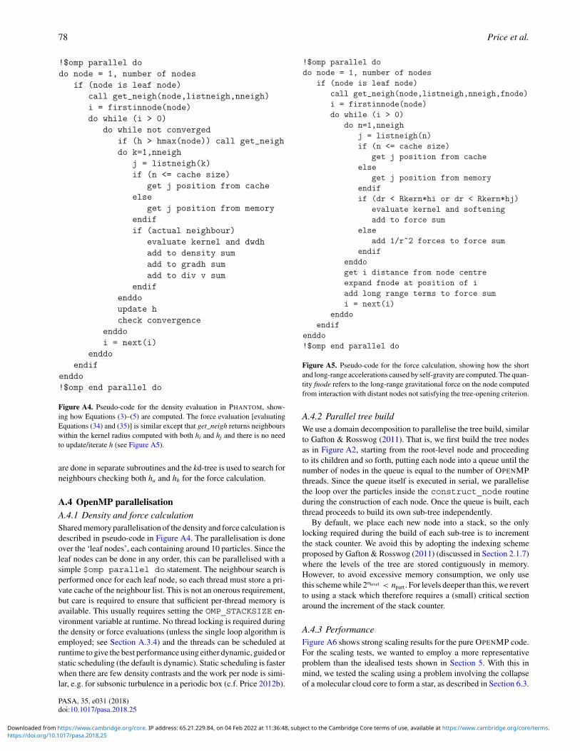
78 Price et al.

!$omp parallel dodo node = 1, number of nodes

if (node is leaf node)call get_neigh(node,listneigh,nneigh)i = firstinnode(node)do while (i > 0)

do while not convergedif (h > hmax(node)) call get_neighdo k=1,nneigh

j = listneigh(k)if (n <= cache size)

get j position from cacheelse

get j position from memoryendifif (actual neighbour)

evaluate kernel and dwdhadd to density sumadd to gradh sumadd to div v sum

endifenddoupdate hcheck convergence

enddoi = next(i)

enddoendif

enddo!$omp end parallel do

Figure A4. Pseudo-code for the density evaluation in PHANTOM, show-ing how Equations (3)–(5) are computed. The force evaluation [evaluatingEquations (34) and (35)] is similar except that get_neigh returns neighbourswithin the kernel radius computed with both hi and hj and there is no needto update/iterate h (see Figure A5).

are done in separate subroutines and the kd-tree is used to search forneighbours checking both ha and hb for the force calculation.

A.4 OpenMP parallelisationA.4.1 Density and force calculationShared memory parallelisation of the density and force calculation isdescribed in pseudo-code in Figure A4. The parallelisation is doneover the ‘leaf nodes’, each containing around 10 particles. Since theleaf nodes can be done in any order, this can be parallelised with asimple $omp parallel do statement. The neighbour search isperformed once for each leaf node, so each thread must store a pri-vate cache of the neighbour list. This is not an onerous requirement,but care is required to ensure that sufficient per-thread memory isavailable. This usually requires setting the OMP_STACKSIZE en-vironment variable at runtime. No thread locking is required duringthe density or force evaluations (unless the single loop algorithm isemployed; see Section A.3.4) and the threads can be scheduled atruntime to give the best performance using either dynamic, guided orstatic scheduling (the default is dynamic). Static scheduling is fasterwhen there are few density contrasts and the work per node is simi-lar, e.g. for subsonic turbulence in a periodic box (c.f. Price 2012b).

!$omp parallel dodo node = 1, number of nodes

if (node is leaf node)call get_neigh(node,listneigh,nneigh,fnode)i = firstinnode(node)do while (i > 0)

do n=1,nneighj = listneigh(n)if (n <= cache size)

get j position from cacheelse

get j position from memoryendifif (dr < Rkern*hi or dr < Rkern*hj)

evaluate kernel and softeningadd to force sum

elseadd 1/r^2 forces to force sum

endifenddoget i distance from node centreexpand fnode at position of iadd long range terms to force sumi = next(i)

enddoendif

enddo!$omp end parallel do

Figure A5. Pseudo-code for the force calculation, showing how the shortand long-range accelerations caused by self-gravity are computed. The quan-tity fnode refers to the long-range gravitational force on the node computedfrom interaction with distant nodes not satisfying the tree-opening criterion.

A.4.2 Parallel tree buildWe use a domain decomposition to parallelise the tree build, similarto Gafton & Rosswog (2011). That is, we first build the tree nodesas in Figure A2, starting from the root-level node and proceedingto its children and so forth, putting each node into a queue until thenumber of nodes in the queue is equal to the number of OPENMPthreads. Since the queue itself is executed in serial, we parallelisethe loop over the particles inside the construct_node routineduring the construction of each node. Once the queue is built, eachthread proceeds to build its own sub-tree independently.

By default, we place each new node into a stack, so the onlylocking required during the build of each sub-tree is to incrementthe stack counter. We avoid this by adopting the indexing schemeproposed by Gafton & Rosswog (2011) (discussed in Section 2.1.7)where the levels of the tree are stored contiguously in memory.However, to avoid excessive memory consumption, we only usethis scheme while 2nlevel < npart . For levels deeper than this, we revertto using a stack which therefore requires a (small) critical sectionaround the increment of the stack counter.

A.4.3 PerformanceFigure A6 shows strong scaling results for the pure OPENMP code.For the scaling tests, we wanted to employ a more representativeproblem than the idealised tests shown in Section 5. With this inmind, we tested the scaling using a problem involving the collapseof a molecular cloud core to form a star, as described in Section 6.3.

PASA, 35, e031 (2018)doi:10.1017/pasa.2018.25






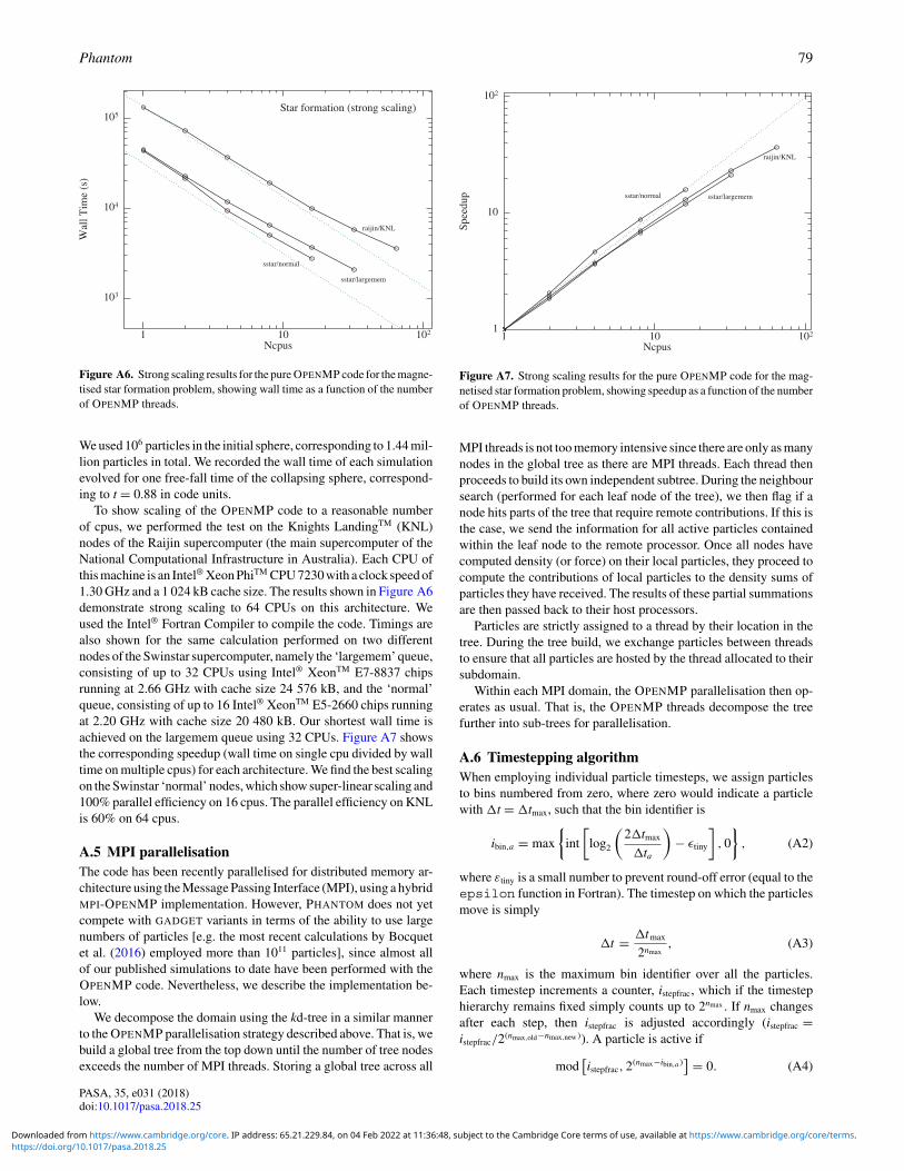
Phantom 79

Figure A6. Strong scaling results for the pure OPENMP code for the magne-tised star formation problem, showing wall time as a function of the numberof OPENMP threads.

We used 106 particles in the initial sphere, corresponding to 1.44 mil-lion particles in total. We recorded the wall time of each simulationevolved for one free-fall time of the collapsing sphere, correspond-ing to t = 0.88 in code units.

To show scaling of the OPENMP code to a reasonable numberof cpus, we performed the test on the Knights LandingTM (KNL)nodes of the Raijin supercomputer (the main supercomputer of theNational Computational Infrastructure in Australia). Each CPU ofthis machine is an Intel® Xeon PhiTM CPU 7230 with a clock speed of1.30 GHz and a 1 024 kB cache size. The results shown in Figure A6demonstrate strong scaling to 64 CPUs on this architecture. Weused the Intel® Fortran Compiler to compile the code. Timings arealso shown for the same calculation performed on two differentnodes of the Swinstar supercomputer, namely the ‘largemem’ queue,consisting of up to 32 CPUs using Intel® XeonTM E7-8837 chipsrunning at 2.66 GHz with cache size 24 576 kB, and the ‘normal’queue, consisting of up to 16 Intel® XeonTM E5-2660 chips runningat 2.20 GHz with cache size 20 480 kB. Our shortest wall time isachieved on the largemem queue using 32 CPUs. Figure A7 showsthe corresponding speedup (wall time on single cpu divided by walltime on multiple cpus) for each architecture. We find the best scalingon the Swinstar ‘normal’ nodes, which show super-linear scaling and100% parallel efficiency on 16 cpus. The parallel efficiency on KNLis 60% on 64 cpus.

A.5 MPI parallelisationThe code has been recently parallelised for distributed memory ar-chitecture using the Message Passing Interface (MPI), using a hybridMPI-OPENMP implementation. However, PHANTOM does not yetcompete with GADGET variants in terms of the ability to use largenumbers of particles [e.g. the most recent calculations by Bocquetet al. (2016) employed more than 1011 particles], since almost allof our published simulations to date have been performed with theOPENMP code. Nevertheless, we describe the implementation be-low.

We decompose the domain using the kd-tree in a similar mannerto the OPENMP parallelisation strategy described above. That is, webuild a global tree from the top down until the number of tree nodesexceeds the number of MPI threads. Storing a global tree across all

Figure A7. Strong scaling results for the pure OPENMP code for the mag-netised star formation problem, showing speedup as a function of the numberof OPENMP threads.

MPI threads is not too memory intensive since there are only as manynodes in the global tree as there are MPI threads. Each thread thenproceeds to build its own independent subtree. During the neighboursearch (performed for each leaf node of the tree), we then flag if anode hits parts of the tree that require remote contributions. If this isthe case, we send the information for all active particles containedwithin the leaf node to the remote processor. Once all nodes havecomputed density (or force) on their local particles, they proceed tocompute the contributions of local particles to the density sums ofparticles they have received. The results of these partial summationsare then passed back to their host processors.

Particles are strictly assigned to a thread by their location in thetree. During the tree build, we exchange particles between threadsto ensure that all particles are hosted by the thread allocated to theirsubdomain.

Within each MPI domain, the OPENMP parallelisation then op-erates as usual. That is, the OPENMP threads decompose the treefurther into sub-trees for parallelisation.

A.6 Timestepping algorithmWhen employing individual particle timesteps, we assign particlesto bins numbered from zero, where zero would indicate a particlewith �t = �tmax, such that the bin identifier is

ibin,a = max

{int

[log2

(2�tmax

�ta

)− εtiny

], 0

}, (A2)

where εtiny is a small number to prevent round-off error (equal to theepsilon function in Fortran). The timestep on which the particlesmove is simply

�t = �tmax

2nmax, (A3)

where nmax is the maximum bin identifier over all the particles.Each timestep increments a counter, istepfrac, which if the timestephierarchy remains fixed simply counts up to 2nmax . If nmax changesafter each step, then istepfrac is adjusted accordingly (istepfrac =istepfrac/2(nmax,old−nmax,new )). A particle is active if

mod[istepfrac, 2(nmax−ibin,a )

] = 0. (A4)

PASA, 35, e031 (2018)doi:10.1017/pasa.2018.25






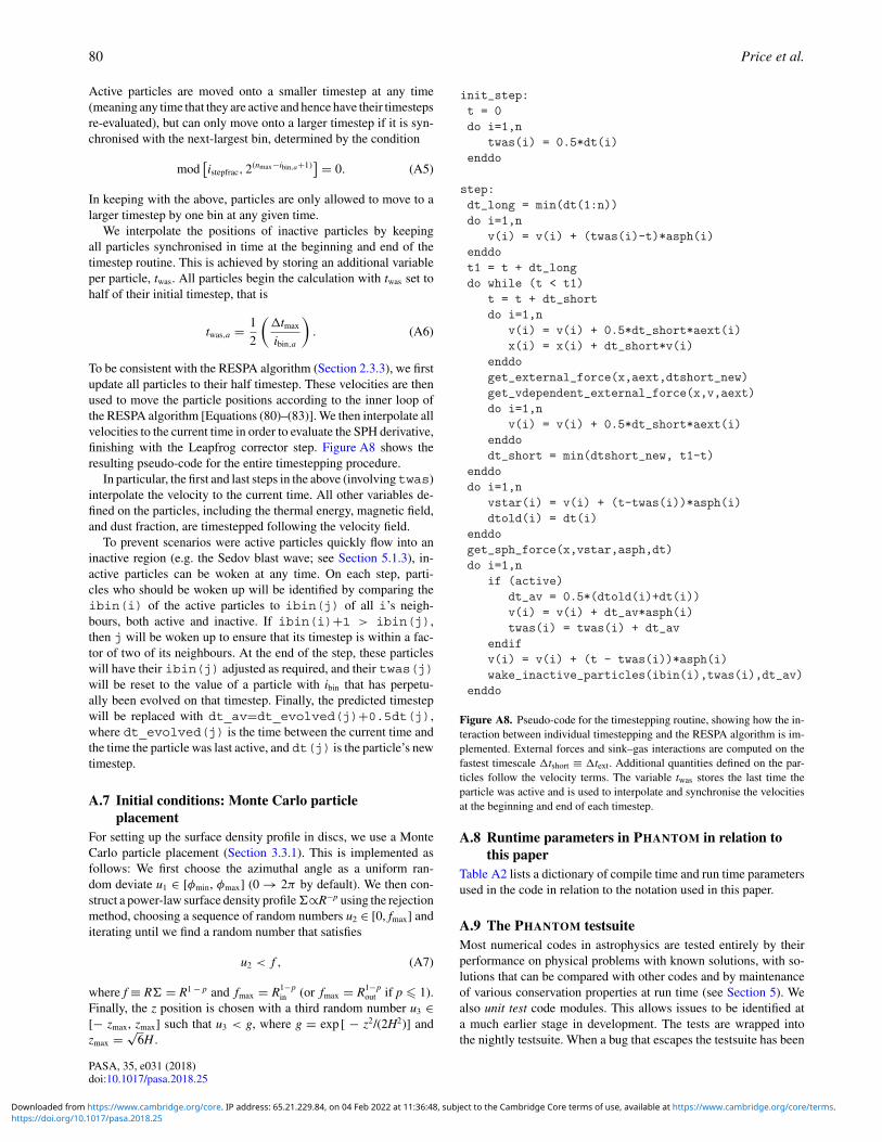
80 Price et al.

Active particles are moved onto a smaller timestep at any time(meaning any time that they are active and hence have their timestepsre-evaluated), but can only move onto a larger timestep if it is syn-chronised with the next-largest bin, determined by the condition

mod[istepfrac, 2(nmax−ibin,a+1)

] = 0. (A5)

In keeping with the above, particles are only allowed to move to alarger timestep by one bin at any given time.

We interpolate the positions of inactive particles by keepingall particles synchronised in time at the beginning and end of thetimestep routine. This is achieved by storing an additional variableper particle, twas. All particles begin the calculation with twas set tohalf of their initial timestep, that is

twas,a = 1

2

(�tmax

ibin,a

). (A6)

To be consistent with the RESPA algorithm (Section 2.3.3), we firstupdate all particles to their half timestep. These velocities are thenused to move the particle positions according to the inner loop ofthe RESPA algorithm [Equations (80)–(83)]. We then interpolate allvelocities to the current time in order to evaluate the SPH derivative,finishing with the Leapfrog corrector step. Figure A8 shows theresulting pseudo-code for the entire timestepping procedure.

In particular, the first and last steps in the above (involvingtwas)interpolate the velocity to the current time. All other variables de-fined on the particles, including the thermal energy, magnetic field,and dust fraction, are timestepped following the velocity field.

To prevent scenarios were active particles quickly flow into aninactive region (e.g. the Sedov blast wave; see Section 5.1.3), in-active particles can be woken at any time. On each step, parti-cles who should be woken up will be identified by comparing theibin(i) of the active particles to ibin(j) of all i’s neigh-bours, both active and inactive. If ibin(i)+1 > ibin(j),then j will be woken up to ensure that its timestep is within a fac-tor of two of its neighbours. At the end of the step, these particleswill have their ibin(j) adjusted as required, and their twas(j)will be reset to the value of a particle with ibin that has perpetu-ally been evolved on that timestep. Finally, the predicted timestepwill be replaced with dt_av=dt_evolved(j)+0.5dt(j),where dt_evolved(j) is the time between the current time andthe time the particle was last active, and dt(j) is the particle’s newtimestep.

A.7 Initial conditions: Monte Carlo particleplacement

For setting up the surface density profile in discs, we use a MonteCarlo particle placement (Section 3.3.1). This is implemented asfollows: We first choose the azimuthal angle as a uniform ran-dom deviate u1 ∈ [φmin, φmax] (0 → 2π by default). We then con-struct a power-law surface density profile �∝R−p using the rejectionmethod, choosing a sequence of random numbers u2 ∈ [0, fmax] anditerating until we find a random number that satisfies

u2 < f , (A7)

where f ≡ R� = R1 − p and fmax = R1−pin (or fmax = R1−p

out if p � 1).Finally, the z position is chosen with a third random number u3 ∈[− zmax, zmax] such that u3 < g, where g = exp [ − z2/(2H2)] andzmax = √

6H .

init_step:t = 0do i=1,n

twas(i) = 0.5*dt(i)enddo

step:dt_long = min(dt(1:n))do i=1,n

v(i) = v(i) + (twas(i)-t)*asph(i)enddot1 = t + dt_longdo while (t < t1)

t = t + dt_shortdo i=1,n

v(i) = v(i) + 0.5*dt_short*aext(i)x(i) = x(i) + dt_short*v(i)

enddoget_external_force(x,aext,dtshort_new)get_vdependent_external_force(x,v,aext)do i=1,n

v(i) = v(i) + 0.5*dt_short*aext(i)enddodt_short = min(dtshort_new, t1-t)

enddodo i=1,n

vstar(i) = v(i) + (t-twas(i))*asph(i)dtold(i) = dt(i)

enddoget_sph_force(x,vstar,asph,dt)do i=1,n

if (active)dt_av = 0.5*(dtold(i)+dt(i))v(i) = v(i) + dt_av*asph(i)twas(i) = twas(i) + dt_av

endifv(i) = v(i) + (t - twas(i))*asph(i)wake_inactive_particles(ibin(i),twas(i),dt_av)

enddo

Figure A8. Pseudo-code for the timestepping routine, showing how the in-teraction between individual timestepping and the RESPA algorithm is im-plemented. External forces and sink–gas interactions are computed on thefastest timescale �tshort ≡ �text. Additional quantities defined on the par-ticles follow the velocity terms. The variable twas stores the last time theparticle was active and is used to interpolate and synchronise the velocitiesat the beginning and end of each timestep.

A.8 Runtime parameters in PHANTOM in relation tothis paper

Table A2 lists a dictionary of compile time and run time parametersused in the code in relation to the notation used in this paper.

A.9 The PHANTOM testsuiteMost numerical codes in astrophysics are tested entirely by theirperformance on physical problems with known solutions, with so-lutions that can be compared with other codes and by maintenanceof various conservation properties at run time (see Section 5). Wealso unit test code modules. This allows issues to be identified ata much earlier stage in development. The tests are wrapped intothe nightly testsuite. When a bug that escapes the testsuite has been

PASA, 35, e031 (2018)doi:10.1017/pasa.2018.25






Phantom 81

Table A2. Various runtime parameters in the code and their relation to this paper.

Quantity Code variable Description Reference

hfact hfact Ratio of smoothing length to particle spacing 2.1.21/�a gradh Smoothing length gradient correction term 2.1.2εh tolh Tolerance in smoothing length–density iterations 2.1.4Fab grkern Scalar part of kernel gradient 2.1.5∂Wab(h)/∂ha dwdh Derivative of kernel with respect to smoothing length 2.1.5K polyk Polytropic constant used for barotropic equations of state 2.2.2utime utime Code time unit (cgs) 2.2.3umass umass Code mass unit (cgs) 2.2.3udist udist Code distance unit (cgs) 2.2.3Equation (24) ipdv_heating Option to turn on/off PdV work term in energy equation 2.2.5shock ishock_heating Option to turn on/off shock heating in energy equation 2.2.5σ decay avdecayconst Decay constant in artificial viscosity switch 2.2.9εv tolv Tolerance on velocity error during timestepping 2.3.1�tmax dtmax Maximum time between output files 2.3.4Racc accradius1 Accretion radius for central potential 2.4.1M binarymassr Binary mass ratio for fixed binary potential 2.4.2Racc, 2 accradius2 Accretion radius for secondary in fixed binary potential 2.4.2k0 RadiationPressure Radiation pressure in Poynting–Robertson drag 2.4.7k1 Redshift Gravitational redshift in Poynting–Robertson drag 2.4.7k2 TransverseDrag Transverse component of Poynting–Robertson drag 2.4.7Em st_energy Energy in turbulent stirring pattern 2.5tdecay st_decay Decay time in turbulent stirring pattern 2.5w st_solweight Solenoidal fraction in turbulent stirring pattern 2.5kmin st_stirmin Minimum wavenumber in turbulent stirring pattern 2.5kmax st_stirmax Minimum wavenumber in turbulent stirring pattern 2.5fsol st_solweightnorm Solenoidal weighting in turbulent stirring pattern 2.5ε h_soft_sinksink Fixed gravitational softening length between sink particles 2.8.1σ c psidecayfac Dimensionless ratio of parabolic to hyperbolic ∇ · B cleaning 2.10.8fclean overcleanfac Multiplier on maximum speed in divergence cleaning 2.10.9ρgrain graindenscgs Intrinsic dust density in cgs units 2.13.6fd damp Damping parameter for relaxing initial particle distributions 3.6

discovered, we have endeavoured to create a unit test to prevent afuture recurrence.

A.9.1 Unit tests of derivative evaluationsThe unit test of the density and force calculations checks that variousderivatives evaluate to within some tolerance of the expected value.To achieve this, the test sets up 100 × 100 × 100 SPH particlesin a periodic, unit cube, and specifies the input variables in termsof known functions. For example, the evaluation of the pressuregradient is checked by setting the thermal energy of each particleaccording to

ua(x, y, z) = 1

2π

[3 + sin

(2πxLx

)+ cos

(2πyLy

)+ sin

(2πzLz

)], (A8)

where Lx, Ly, and Lz are the length of the domain in each direction andthe positions are relative to the edge of the box. We then compute theacceleration according to (34) with the artificial viscosity and otherterms switched off, assuming an adiabatic EOS [Equation (25)] withρ = constant. We then test that numerical acceleration on all 106

particles is within some tolerance of the analytic pressure gradientexpected from (341), namely

−∇Pa

ρa(x, y, z) = −(γ − 1)∇ua(x, y, z), (A9)

where typically we use a tolerance of 10−3 in the relative error E(x)= |x − xexact|/xexact.

This procedure is repeated for the various derivatives of velocity,including the velocity divergence, curl, and all components of thestrain tensor. We also test the artificial viscosity terms this way—checking that they translate correctly according to (119)—as well asthe magnetic field derivatives and time derivatives, magnetic forces,artificial resistivity terms, physical viscosity terms, time derivativesof the dust fraction, and the time derivative of the velocity divergencerequired in the viscosity switch. We perform each of these tests alsofor the case where derivatives are evaluated on only a subset of theparticles, as occurs when individual particle timesteps are employed.

We additionally check that various conservation properties aremaintained. For example, energy conservation for hydrodynamicsrequires (37) to be satisfied. Hence, we include a test that checksthat this summation is zero to machine precision. Similar tests areperformed for magnetic fields, and for subsets of the forces thatbalance subsets of the thermal energy derivatives (e.g. the artificialviscosity terms).

A.9.2 Unit tests of sink particlesUnit tests for sink particles include (i) integrating a sink particlebinary for 1 000 orbits and checking that this conserves total energyto a relative error of 10−6 and linear and angular momentum to ma-chine precision; (ii) setting up a circumbinary disc of gas particlesevolved for a few orbits to check that linear and angular momen-tum and energy are conserved; (iii) checking that circular orbits arecorrect in the presence of sink-sink softening; (iv) checking thataccreting a gas particle onto a sink particle conserves linear and

PASA, 35, e031 (2018)doi:10.1017/pasa.2018.25






82 Price et al.

angular momentum, and that the resulting centre of mass position,velocity, and acceleration are set correctly (c.f. Section 2.8.2); and(v) checking that sink particle creation from a uniform sphere of gasparticles (Section 2.8.4) succeeds and that the procedure conserveslinear and angular momentum.

A.9.3 Unit tests of external forcesFor external forces, we implement general tests that can be appliedto any implemented external potential: (i) we check that the acceler-ation is the gradient of the potential by comparing a finite differencederivative of the potential, �, in each direction to the accelerationreturned by the external force routine; and (ii) we check that the rou-tines to solve matrix equations for velocity-dependent forces (e.g.Sections 2.4.5–2.4.7) agree with an iterative solution to the Leapfrogcorrector step [Equation (69)].

A.9.4 Unit tests of neighbour finding routinesIn order to unit test the neighbour finding modules (Section 2.1.7),we set up particles in a uniform random distribution with randomlyassigned smoothing lengths. We then check that the neighbour listcomputed with the treecode agrees with a brute-force evaluation ofactual neighbours. We also perform several sanity checks (i) that nodead or accreted particles appear in the neighbour list; (ii) that allparticles can be reached by traversing the tree or link list structure;(iii) that nodes tagged as active contain at least one active particle andconversely that (iv) inactive cells contain only inactive particles; (v)that there is no double counting of neighbours in the neighbour lists;and (vi) that the cached and uncached neighbour lists are identical.We further check that particle neighbours are found correctly inpathological configurations, e.g. when all particles lie in a 1D linealong each of the coordinate axes.

A.9.5 Unit tests of timestepping and periodic boundariesAs a simple unit test of both the timestepping and periodic bound-aries, we set up 50 × 50 × 50 particles in a uniform periodic boxwith a constant velocity (vx = vy = v z = 1) along the box diagonal.We then evolve this for 10 timesteps and check that the density oneach particle remains constant and that the acceleration and othertime derivatives remain zero to machine precision.

A.9.6 Unit tests of file read/writeWe check that variables written to the header of the (binary) outputfiles are successfully recovered by the corresponding read routine,and similarly for the particle arrays written to the body of the file.This quickly and easily picks up mistakes made in reading/writingvariables from/to the output file.

A.9.7 Unit tests of kernel moduleWe ensure that calls to different kernel routines return the sameanswer, and check that gradients of the kernel and kernel softeningfunctions returned by the routines are within some small toleranceof a finite difference evaluation of these gradients.

A.9.8 Unit tests of self-gravity routinesIn order to unit test the treecode self-gravity computation(Section 2.12), we (i) check that the Taylor series expansion of the

force on each leaf node matches the exact force for a particle placedclose to the node centre; (ii) that the Taylor series expansion ofthe force and potential around the distant node are within a small(∼10−5) tolerance of the exact values; (iii) that the combined expan-sion about both the local and distant nodes produces a force withina small tolerance of the exact value; and finally (iv) that the gravita-tional force computed on the tree for a uniform sphere of particlesis within a small tolerance (∼10−3) of the force computed by directsummation.

A.9.9 Unit tests of dust physics

We unit test the dust modules by first performing sanity checksof the dust–gas drag routine—namely that the transition betweenStokes and Epstein drag is continuous and that the initialisationroutine completes without error. We then perform a low-resolutionDUSTYBOX test (Section 5.9.1), checking the solution matches theanalytic solution as in Figure 46. For one-fluid dust, we performa low-resolution version of the dust diffusion test (Section 5.9.3),checking against the solution at every timestep is within a smalltolerance of the analytic solution. Dust mass, gas mass, and energyconservation in the one-fluid dust derivatives are also checked au-tomatically.

A.9.10 Unit tests of non-ideal MHD

We perform three unit tests on non-ideal MHD. The first is thewave damping test (see Section 5.7.1). This test also uses the super-timestepping algorithm to verify the diffusive [Equation (202) butconsidering only Ohmic resistivity and ambipolar diffusion] andminimum stable timesteps [Equation (72)], but then evolves thesystem on the smallest of the two timesteps. The second test is thestanding shock test (see Section 5.7.2). This test is also designedas a secondary check on boundary particles. Both tests used fixedcoefficients for the non-ideal terms, and for speed, both tests areperformed at much lower resolutions than presented in the paper.The third test self-consistently calculates the non-ideal coefficientsfor given gas properties.

A.9.11 Other unit tests

Various other unit tests are employed, including sanity checks of in-dividual timestepping utility routines, checking that the barotropicEOS is continuous, of the Coriolis and centrifugal force routines,checks of conservation in the generalised Newtonian potential(Section 2.4.6), of the routine to revise the tree, and of the fastinverse square root routines.

A.9.12 Sedov unit test

As a final ‘real’ unit test, the code performs a low-resolution (163)version of the Sedov blast wave test (Section 5.1.3). We check thatenergy and momentum are conserved at a precision appropriate tothe timestepping algorithm (for global timesteps, this means mo-mentum conservation to machine precision and energy conservationto �E/E0 < 5 × 10−4; for individual timesteps, we ensure linear mo-mentum conservation to 2 × 10−4 and energy conservation to 2 ×10−2).

PASA, 35, e031 (2018)doi:10.1017/pasa.2018.25






phantom: a smoothed particle hydrodynamics and

Documents