singleparticle treatment of quantum stochastic resonance
TRANSCRIPT
Physica A 275 (2000) 505–530www.elsevier.com/locate/physa
Single-particle treatment of quantum stochasticresonance
V.J. Menon, N. Chanana ∗, Y. SinghDepartment of Physics, Banaras Hindu University, Varanasi 221005, India
Received 15 April 1999
Abstract
We �rst consider a test particle subjected to the simultaneous in uence of a double-well mean�eld, thermal velocity distribution, external white noise and sinusoidal modulation. Within apath-integral framework the resulting power spectrum along with the signal-to-noise ratio (SNR)are expressed perturbatively in terms of the unperturbed eigenfunctions n and eigenvalues En,permitting us to demonstrate the existence of the phenomenon of quantum stochastic resonance(SR) in the dissipationless case. Next, we show that with the help of suitable transformations(viz., a complex Fourier frequency or a scaled-up potential) systems with weak friction or strongdamping can be approximately mapped onto the dissipationless case. This yields a convenientmethod for studying frictional SR because the n’s and En’s can still be generated through ashort-time propagator. Our formulation is illustrated numerically by displaying the variation ofthe SNR with the external noise strength and comparing the results vis-�a-vis those obtained fromclassical stochastic simulation and quantum bath models. The usefulness of the single-particleapproach to analyze the quantum SR phenomenon is emphasized. c© 2000 Elsevier ScienceB.V. All rights reserved.
PACS: 05.04.+ j
1. Introduction
In recent years many workers have become increasingly interested in noise-induced,resonance-like e�ects in nonlinear systems. The most extensively studied phenomenonof this kind is the stochastic resonance (SR) [1] which is a cooperative e�ect ofnonlinearity, periodicity and stochasticity, resulting in an enhancement of small coherentsignals by random noise. This phenomenon has been the subject of many investigationsin classical systems studied via analytical=numerical=analog solutions of the Langevin
∗ Correspondence address: 826 16th St South, Birmingham, AL 35205, USA.E-mail address: [email protected] (V.J. Menon)
0378-4371/00/$ - see front matter c© 2000 Elsevier Science B.V. All rights reserved.PII: S 0378 -4371(99)00357 -X
506 V.J. Menon et al. / Physica A 275 (2000) 505–530
equation [2,3], overdamped Rayleigh equation [4] and the Fokker–Planck equation [5,6].The SR concept can also be extended to the transmission of aperiodic signals byneuronal ensembles [7] or by binary channels [8] and to the synchronization of amicromaser [9]. The role of quantum uctuations on SR has only started to be exploredrecently using the elaborate bath models [10–13].There are three commonly used ways of characterizing the SR in the literature
[1–13] especially in the context of the double-well potential which mimics bistablesystems. These are the study of the �rst passage time across the barrier, calculation ofthe position autocorrelation function, and analysis of the power spectrum yielding thesignal-to-noise ratio (SNR). It has been established that the SR disappears when thedi�usion constant D tends either to zero or in�nity. The SR, however, survives withrespect to wide variations in the modulation strength, signal frequency, temperatureand the coe�cient of friction. In the generation of SR, an important role is played bythe fact that the e�ective double well becomes asymmetric either intrinsically or onaccount of the modulation.The aim of the present paper is to consider a quantum particle described by the
Feynman path integrals [14] and study the variation of the SNR with respect to thestrength of the externally applied white noise. The path integral technique is elegantand easy to the use since it involves c-number actions in the construction of theprobability densities. On the other hand, the formally equivalent quantum stochasticLiouville equation approach [15,16] is more di�cult to use since it involves q-numbercommutators in the construction of the reduced density matrix. Results are derived inthe limits of weak noise - small friction and also weak noise-arbitrary damping byappealing to a recently developed concept of the random motion [17] executed by anotherwise conservative quantum particle. We shall adopt a single-particle description ofquantum SR rather than the comprehensive bath model treatment. The motivations fordoing this are threefold, viz. (i) the single-particle approach has been very commonwith the classical theories [1–9] of the SR, (ii) it leads to considerable analyticalsimpli�cation in the theoretical formalism, and (iii) it is particularly useful to dealwith variations of the external noise strength.The present paper is organized as follows. In Section 2 we formulate the analytical
tools for handling perturbatively the SNR in the case of zero dissipation. The fact thatthe stochastic resonance exists in quantum dissipationless random motion (QDRM)was shown recently [17]. In the same section hint is taken from earlier literatureon Brownian movement [18,19] to justify the averaging over an input Maxwellian.The importance of QDRM is that frictional stochastic dynamics can be mapped ontothe former so that the usual methods of path integration [20] can be employed. InSection 3 we show how this mapping is achieved in the weak friction case for a sys-tem described by the Bateman–Caldirola–Kanai dissipational Lagrangian [21–24] andillustrate the ideas numerically. It will be observed that the short-time propagatormethod [20] is numerically much easier than the elaborate matrix-multiplication tech-nique [25]. Next, in Section 4 we carry out a mapping of a motion under strongfriction onto a dissipationless dynamics by introducing the concept of the scaled-up
V.J. Menon et al. / Physica A 275 (2000) 505–530 507
potential [26] and illustrate quantum SR graphically. Finally, our main conclusions aresummarized in Section 5 including a hint on possible applications [27–29].
2. SNR in quantum dissipationless random motion
2.1. Preliminaries
During a time interval ta=0¡t¡ tb consider the motion of a particle having mass m,position x, velocity v, binding potential energy VR ; and mean �eld force FR=−@[email protected] T be the absolute temperature of the medium and � = (kT )−1 with k being theBoltzmann constant. We set up the unperturbed action
SVxba =
∫dt
(mv2
2− VR
); (1)
where the time integration always runs from ta = 0 to tb ¿ 0. In order to deal withthe stochastic resonance problem we introduce a position-independent Gaussian randomforce f and periodic modulation force y speci�ed by
〈f(t)f(t′)〉= C�(t − t′); �[f] = exp{−(2C)−1
∫dt f2
}; (2a)
y = ymax cos (!st + �) ; (2b)
where C is the autocorrelation strength, � the white noise distributional, ymax the am-plitude of modulation, and � its phase. It may be stressed here that in the quantumcase the random force should be a time-dependent operator having a complex auto-correlation function which makes its practical application very di�cult. We assume fto be a c-number white noise because such an assumption has been very common instochastic dynamics and, furthermore, it greatly facilitates analytical calculations.Upon including both f and y in the action the full Feynman propagator [14] between
the points xa and xb becomes
Kxbxa =∫Dx exp
{i˝
[SVxba +
∫dt x(f + y)
]}: (3a)
The input wave function of the particle at ta = 0 is taken as a minimum uncertaintypacket of width �0, mean position x0, and average momentum p0, i.e.,
0(xa) =1
(2��20)1=4exp
{i˝xap0 −
(xa − x0)2
4�20
}: (3b)
Then, for a given pro�le of the noise f and modulation y, the conditional probabilitydensity of locating the particle at point xb at time tb is given by
PQ =∣∣∣∣∫ +∞
−∞dxa Kxbxa
0(xa)∣∣∣∣2
; (3c)
where the su�x Q stands for quantum.
508 V.J. Menon et al. / Physica A 275 (2000) 505–530
2.2. Statistical averaging
The function PQ must now be averaged over the noise distributional �[f] andover the Maxwellian distribution of the initial momentum p0. As was pointed out inRef. [17] the statistically averaged probability density may be written compactly as
P = Tr[�] =∫ +∞
−∞dxa
∫ +∞
−∞dx′a xax′a�x′axa ; (4)
where
xax′a=(2��0)−1=2 exp[−m(xa−x′a)
2=(2˝2�)− (xa − x0)2=4�20− (x′a−x0)2=4�20](5a)
and
�x′axa =∫Dx
∫Dx′ exp
[i˝
{SVxba − SVx′
ba′ + (iC=2˝)
×∫dt(x − x′)2 +
∫dt(x − x′)y
} ]: (5b)
Here the x(x′) path runs from the point xa(x′a) at time ta to the point xb at time tb.Some comments on Eqs. (4) and (5) are now in order:(i) The basic trick to average over the noise distribution is given in the book by
Feynman and Hibbs [14] which allows the white noise case to be treated exactly.This is, of course, analogous to the corresponding treatment in terms of cumu-lants via the stochastic Liouville approach [16]. However, in either case furthersimpli�cation of the binary propagator �x′axa will require the use of some approx-imation such as perturbation if the binding potential VR is more complicated thana harmonic oscillator.
(ii) A major step taken by us is the averaging over an input Maxwellian velocitydistribution which results in the appearance of the nontrivial factor xax′a . Clearly,this corresponds to an equilibrium initial condition at the ambient temperature Tand its choice is quite standard. In fact, such a velocity averaging was �rst doneby Chandrasekhar [18] and later by the present authors [19] in the context ofclassical and quantum Brownian probabilities, respectively.
2.3. Perturbative treatment
Now suppose that the noise and modulation are both weak, i.e., Cd20tb=˝2.1 andymax.Cd0=˝ where d0 is some characteristic length of the problem (e.g., width of thepotential well or linear size of the ground-state wave function). Then we can expand theintegrand of the binary propagator �x′axa in powers of C and y, neglecting o(C2) ando(y2) terms but retaining the o(Cy) cross term. Employing the standard eigenfunctionexpansion for the unperturbed propagator∫
Dx exp{i˝S
Vxba
}=∑n
n(xb) ?n (xa) e
−iEn(tb−ta)=˝ (5c)
V.J. Menon et al. / Physica A 275 (2000) 505–530 509
in the evaluation of �x′axa we arrive at the series
P =∑mn
mn{�V
nm + �Cnm + �y
nm + �Cy¡nm + �Cy¿
nm
}: (6)
Here n is the unperturbed eigenfunction (corresponding to potential VR) with energyeigenvalue En. The �nm
′s are space–time-dependent functions representing various typesof contributions to the averaged probability density. Before identifying the �nm
′s wemay o�er a preliminary justi�cation for retaining the o(Cy) term but ignoring theo(C2) and o(y2) contributions, which are formally of the same order of magnitude inthe expansion of Eq. (5b). While analyzing the power spectrum later in Section 2.7 itwill be found that the signal part arises from the interference of �Cy¡ + �Cy¿ withother terms, the background part will come from |�V
nm+�Cnm|2 while the o(y2) can be
omitted. We shall return to this point again after Eq. (30).
2.4. Identi�cation of � ’s
(i) Mean-�eld contribution arising from the SVxba − SVx′
ba′ terms in Eq. (5) is
�Vnm = gV
nm n(xb) m(xb)hVnm(tb) ; (7a)
where
gVnm = 1; hV
nm(tb) = cos(!nmtb) ; (7b)
!nm = (En − Em)=˝ : (7c)
(ii) Noise contribution arising from the C(x − x′)2 term in Eq. (5) is
�Cnm =
−C2˝2
∑lk
gCnm;lk l(xb) k(xb)hC
nm;lk(tb) ; (8a)
where
gCnm;lk = F (2)nl �km + �nlF
(2)km − 2F (l)nl F
(1)km ; (8b)
hCnm;lk(tb) =
sin(!nmtb)− sin(!lk tb)(!nm − !lk)
; (8c)
F (�)nl =∫ +∞
−∞dx n(x)x� l(x) : (8d)
(iii) Modulation contribution arising from the (x − x′)y term in Eq. (5) is
�Ynm =
1˝∑lk
gynm;lk l(xb) k(xb)h
ynm;lk(tb) ; (9a)
510 V.J. Menon et al. / Physica A 275 (2000) 505–530
where
gynm;lk = F (1)nl �km − �nlF
(1)km ; (9b)
hnm;lk(tb) =∫ tb
0dt2 y(t2) sin(�2) (9c)
with
�2 = !lk tb + (!nm − !lk)t2 : (9d)
(iv) Noise-modulation interference contribution of the prior type arising when the timet of (x − x′)2 path is earlier than the time t2 of y in Eq. (5) is given by
�Cy¡nm =
C2˝3
∑qlkp
gCy¡nm;qp;lk l(xb) k(xb)h
Cy¡nm;qp;lk(tb) ; (10a)
where
gCy¡nm;qp;lk = gC
nm;qpgyqp;lk ; (10b)
hCy¡nm;qp;lk(tb) =
1(!nm − !qp)
∫ tb
0dt2 y(t2) {cos(�¡
2 )− cos(�¡2 )} (10c)
with
�¡2 = !lk tb + (!nm − !lk)t2 (10d)
and
�¡2 = !lk tb + (!qp − !lk)t2 : (10e)
(v) Noise-modulation interference contribution of the post type arising when the timet of (x − x′)2 path is later than the time t2 of y in Eq. (5) is written as
�Cy¿mn =
C2˝3
∑qlkp
gCy¿nm;qp;lk l(xb) k(xb) h
Cy¿nm;qp;lk(tb) ; (11)
where
gCy¿nm;qp;lk = gC
qp;lk gynm;qp ; (11a)
hCy¿nm;qp;lk(tb) =
1(!qp − !lk)
∫ tb
0dt2 y(t2){cos(�¿
2 )− cos(�¿2 )} (11b)
with
�¿2 = !qp tb + (!nm − !qp) t2 (11c)
and
�¿2 = !lk tb + (!nm − !lk)t2 : (11d)
V.J. Menon et al. / Physica A 275 (2000) 505–530 511
2.5. Averaged trajectory and the fourier transformation
Now, we turn to the construction of the stochastically averaged trajectory
x(tb) =∫ +∞
−∞dxb xbP; 06tb6∞ : (12a)
Remembering the formula of P in terms of the �’s (cf. Eqs. (6)–(11)) the evaluation ofx(tb) is facilitated by the observation that
∫ +∞−∞ dxb xb l(xn) k(xb) =F (1)lk . The Fourier
transform of the trajectory is introduced via
x∼(!) =∫ ∞
0dtb x(tb) ei!tb ; ! real : (12b)
The time integration here can be carried out with the help of the h function appearingin Eqs. (7)–(11). This leads to again a sum of �ve terms in analogy with Eq. (6), viz.,
x∼(!) = x∼V (!) + x∼
C(!) + x∼y(!) + x∼
Cy¡(!) + x∼Cy¿(!) : (13)
In the sequel, we suppress the argument !; rather keeping ! �xed we shall regard theRHS of Eq. (13) as a function of the noise strength C.
2.6. Identi�cation of various fourier terms
The contributions of various terms in Eq. (13) are as follows, assuming that ! neverequals 0; !s or !nm:(i) Mean �eld contribution:
x∼V =
∑mn
mng∼VnmF
(1)nm
i!(!2 − !2nm)
; (14a)
!nm = (En − Em)=˝ : (14b)
(ii) Noise contribution:
x∼C =
C2˝2
∑mnlk
mngCnm;lkF
(1)lk
[!2 + !nm!lk
(!2 − !2nm)(!2 − !2lk)
]: (15)
(iii) Modulation contribution:
x∼y =
1˝∑mn
mngynmF
(1)lk h∼
ynm;lk ; (16a)
h∼ynm;lk = H (!nm |!|!lk) : (16b)
(iv) Noise-modulation interference contribution of prior type:
x∼Cy¡ =
C2˝3
∑mnklpq
mn gCy¡nm;qp;lkF
(1)lk h∼
Cy¡nm;qp;lk ; (17a)
gCy¡nm;qp;lk = gC
nm;qp gyqp;lk ; (17b)
512 V.J. Menon et al. / Physica A 275 (2000) 505–530
h∼Cy¡nm;qp;lk =
@G@!nm
(!nm|!|!lk) if !nm = !qp ;
G(!nm|!|!lk)− G(!qp|!|!lk)!nm − !qp
if !nm 6= !qp :(17c)
(v) Noise-modulation interference contribution of post type:
x∼Cy¿(!) =
C2˝3
∑mnklpq
mn gCy¿nm;qp;lkF
(1)lk h∼
Cy¿nm;qp;lk ; (18a)
gCy¿nm;qp;lk = gy
nm;qp gCqp;lk ; (18b)
h∼Cy¿nm;qp;lk =
@G@!qp
(!nm|!|!qp) if !qp = !lk ;
G(!nm|!|!qp)− G(!nm|!|!lk)!qp − !lk
if !qp 6= !lk :
(18c)
In the preceding expressions we have introduced additional symbols G and H whichare de�ned as follows. Given a set of frequencies !U; !; !L we construct from themodulation y
y∼(!) =
∫ ∞
0dt y ei!t
= ymax
[i! cos�− !s sin�
!2 − !2s
]; (19)
y′(!) = @ y∼(!)=@!
=−ymax!2
(!2 − !2s )2
[2!s!sin�+ i
(1 +
!2s!2
)cos�
]; (20)
�(!u |!) = 12{y(!+ !u) + y(!− !u)} ; (21)
�(!u |!) = 12i{y(!+ !u)− y(!− !u)} ; (22)
�′(!u |!) = @�@!
=12{y′(!+ !u) + y′(!− !u)} ; (23)
�′(!u |!) = @�@!
=12i{y′(!+ !u)− y′(!− !u)} ; (24)
G(!u |!|!L) = !L�(!u |!) + i!�(!u |!)(!2 − !2L)
; (25)
H (!u |!|!L) = −!L�(!u |!) + i!�(!u |!)(!2 − !2L)
; (26)
V.J. Menon et al. / Physica A 275 (2000) 505–530 513
@G@!u
=−!�′(!u |!)− i!L�′(!u |!)
(!2 − !2L); (27)
@G@!L
=(!2 + !2L) �(!u |!) + 2i!!L�(!u |!)
(!2 − !2L)2: (28)
2.7. Power spectrum and signal-to-noise ratio
From Eq. (13) we set up the power spectrum as
S = | x∼ |2 = Ss + Sb ; (29)
where the signal part Ss and the background part Sb of the power spectrum are de�nedas follows. Let xCy = xCy¡ + xCy¿, then
Ss = | x∼ Cy|2 + 2Re(x∼ V?x∼
Cy) + 2Re(x∼C?
x∼y)
+2Re(x∼C?
x∼Cy) + 2Re(x∼
y?x∼
Cy) (30a)
and
Sb = | x∼ V |2 + | x∼ C |2 + 2Re(x∼ V?x∼
C) : (30b)
The signal-to-noise ratio (SNR) is de�ned by
R= Ss=Sb : (30c)
At this stage we pause to make several important remarks on Eqs. (29) and (30). Whiledescribing a stochastic resonance one has to adopt a suitable convention regarding thesignal part Ss and the background part Sb. In the classical power spectrum of McNamaraand Wiesenfeld [4] the coe�cient of �(!− !s) was taken to be Ss; we cannot adoptthis criterion because !− !s never vanishes in our analysis. We have rather imposedthe crucial requirement that Ss must vanish when either C or y becomes zero whichexplains why x∼
Cy appears in Eq. (30a).
As far as the background Sb is concerned, expression (30b) is fairly unambiguous.Note that the square of the pure modulation term | x∼ y|2 has been dropped while writingEq. (30) because it cannot qualify either for Ss or Sb. The stochastic resonance ofdissipationless random motion is searched by looking at the variation of R with noisecorrelator C keeping other parameters �xed.
2.8. Numerical illustration
In order to illustrate the above theory we take a symmetric double-well potentialVR = −0:4x2 + 0:05x4 in the ˝ = m = d0 = 1 units. The �rst 15 eigenvalues andeigenfunctions were generated by using the matrix-diagonalization method of Sethia etal. [20]. Keeping �; x0; �0; ymax; �; !s and ! suitably �xed, we varied the noise
514 V.J. Menon et al. / Physica A 275 (2000) 505–530
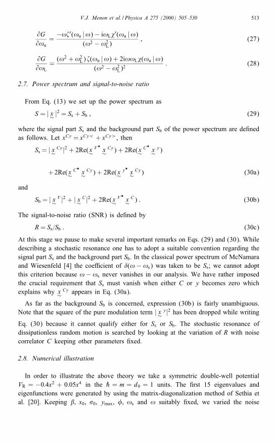
Fig. 1. Variation of the signal-to-noise ratio as a function of the noise strength. The model used to get thequantum SR is dissipationless random motion. Values of other parameters are indicated on the diagram. Asymmetric double-well potential VR =−0:4x2 + 0:05x4 has been chosen.
strength over the range 06C60:1 and computed the signal-to-noise ratio R fromEqs. (30) as a function of C. The whole procedure was repeated for other choicesof the input parameters bearing in mind two precautions, viz., ˝!s and ˝! shouldbe much less than the energy-level separation, and the modulation potential amplitudethough small compared to the well-depth should be strong enough to cause a transitof the particle from one well to the other.Fig. 1 shows our results corresponding to the parameter set
�= 10:0; x0 =−2; �0 = 0:88; 0:0016ymax60:01 ;
�= 90◦; !s = 0:126; != 0:063 ;
assuming that the initial wavepacket is centered at the mid point of the left well. Aclear signature of the stochastic resonance is seen as R increases with C upto a peakvalue (centered at Cr = 0:009 for ymax = 0:001) and falls-o� rapidly as C becomesstill higher. Also when ymax was changed to 0:01 the location Cr of the peak remainedunaltered. Practical examples of systems which execute QDRM and to which the abovetheory can be applied will be mentioned towards the end in Section 5.
V.J. Menon et al. / Physica A 275 (2000) 505–530 515
3. SR via the Bateman–Caldirola–Kanai Lagrangian : weak friction case
3.1. Preliminaries
In this section we examine the description of quantum SR within a phenomenologicalfrictional single-particle philosophy. As is customary, the dissipative force is assumedlinear in velocity, friction with the surrounding is characterized by an empirical constant , and the simultaneous in uence of binding, noise, and modulation is invoked via thee�ective potential
V = VR − xf − xy : (31a)
It is known that the classical Langevin-like equation of motion follows from theBateman–Caldirola–Kanai (BCK) Lagrangian [21–23]
L= G2(mv2=2− V ); G = e t=2 : (31b)
Although the modern fashionable way to introduce dissipation in statistical mechanicsis through the quantum bath model [24] yet the BCK approach remains useful to treatproblems such as the damped quantum harmonic oscillator [22] and squeezed wavepackets in quantum optics [23] using the single-particle viewpoint.
3.2. Quantization
Obviously, the presence of the explicitly time-dependent factor G in Eq. (31b) makesit very di�cult either to solve the Schrodinger equation or to evaluate the path integral.As a �rst step towards overcoming the said di�culty we note that the classical dissipa-tional Langevin equation (having a v term) can be cast into a classical dissipationlessequation of motion by performing a canonical transformation [22]
�x = Gx; �v= G(v+ x=2) : (32)
The Lagrangian in the new variables becomes
�L=m �v 2
2− �V − d ��
dt; (33)
where
�V = G2(V − m 2x2=8); ��= m �x 2=4 : (34)
The quantum probability density de�ned in Eq. (3c) can now be rewritten as
PQ = Gb �PQ; Gb = e tb=2 ; (35)
�PQ =∣∣∣∣∫ +∞
−∞d �xa �Kba 0( �xa)
∣∣∣∣2
(36)
where the coe�cient Gb ensures correct normalization and �Kba is the propagator be-tween the points �xa = xa and �xb = Gbxb computed with the help of the Lagrangian �L.
516 V.J. Menon et al. / Physica A 275 (2000) 505–530
Further investigation of the properties=applications of transformation (32)–(36) canbe carried out by emphasizing the following points: (i) the term d ��=dt in Eq. (33) beinga total derivative cannot alter the classical trajectories; (ii) the piece G2(V −m 2x2=8)represents a time-independent mean �eld in the �x variable if V was a harmonic oscil-lator in the x variable; (iii) in the case of more complicated binding potentials V suchas the double well the piece G2(V − m 2x2=8) remains explicitly time dependent inthe �x variable so that evaluation of �Kba by the usual Feynman–Hibbs [14] techniquesbecomes troublesome.
3.3. Mapping onto dissipationless motion
In order to overcome the trouble mentioned above we argue as follows. Due to the
function G the integrand of the new action �S =∫ �b�a dt �L receives exponentially growing
contributions for times obeying tb ¿ 1. Because of this, propagator phase exp{i �S=˝}starts oscillating very rapidly. Therefore, as far as time-integrals over the probabilitydensity PQ (cf. Eq. (35)) are concerned, the propagator �Kba of Eq. (36) contributessigni�cantly at times tb ¡ 1. This approximation obviously becomes better, the weakeris the friction, e.g. in a double-well problem it is satis�ed when
. ; (37)
where is the angular frequency of the potential barrier. Replacing now G inEqs. (33) and (34) by unity we �nd that �Kba becomes the same functional formof the new variables �xb; �xa; tb as was Kba of the old variables xb; xa; tb.
3.4. Stochastic averaging and Fourier transform
In analogy with our earlier treatment of quantum dissipationless random motionthe averaging of Eq. (35) over the white noise distributional and input momentumdistribution yields
P = Gb �P = GbTr[ � ��] ; (38)
where the elements of the matrices � and �� are the bar-variable counterparts, ofEqs. (5a) and (5b). The stochastically averaged old trajectory is, by de�nition,
x(tb) =∫ +∞
−∞dxb xbP
=∫ +∞
−∞G−1
b d �xb G−1b �xb Gb �Pb = G−1
b �x(tb) ; (39)
where �x(tb) is the stochastically averaged trajectory entirely in bar variables. Hence theFourier transform of the original trajectory reads
x∼(!) =∫ ∞
0dtb ei!tb :e− tb=2 �x(tb)
= �x∼(!+ i =2) ; (40)
V.J. Menon et al. / Physica A 275 (2000) 505–530 517
where �x∼ is the Fourier transform of the bar trajectory evaluated at the complex point
!+ i =2.Eq. (40) is the central result of this section. We have demonstrated that the original
analysis of the power spectrum (cf. Eqs. (29) and (30)) done for the case of quantumdissipationless random motion again goes through. The only e�ect of weak frictionis that one has to use the Lagrangian �L (with G set equal to unity) and replace theFourier frequency by (!+ i =2). The eigenvalues and eigenfunctions for the potentialVR − m 2x2=8 are generated using the method of Sethia et al. [20].
3.5. Numerical work
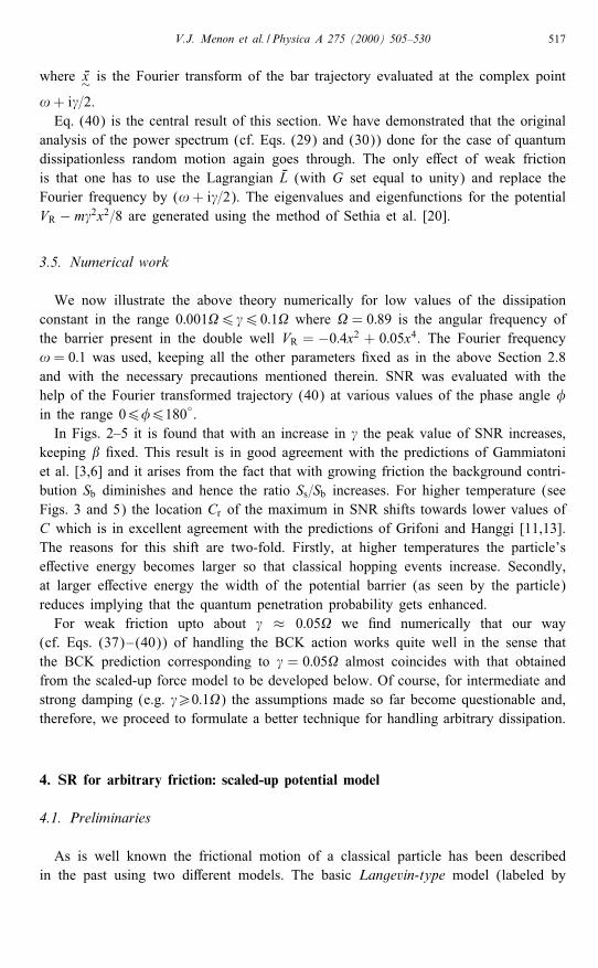
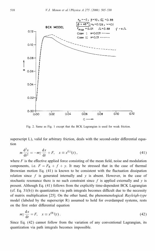
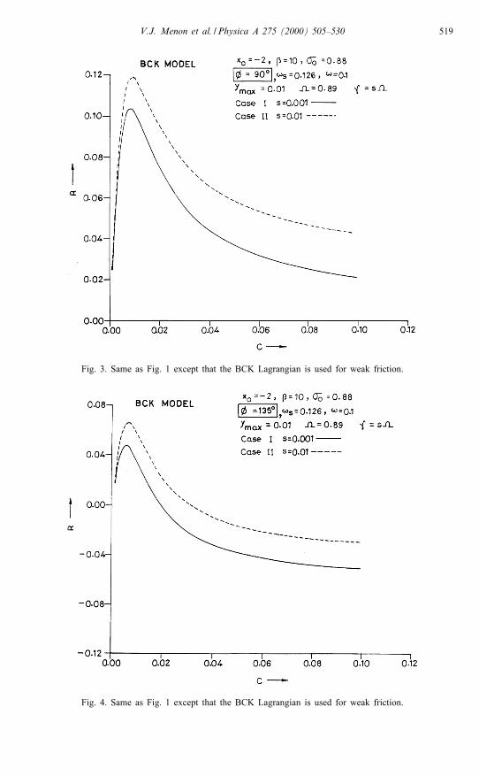
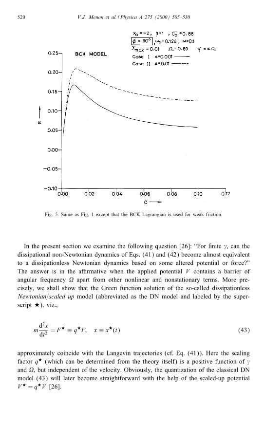
We now illustrate the above theory numerically for low values of the dissipationconstant in the range 0:0016 60:1 where = 0:89 is the angular frequency ofthe barrier present in the double well VR = −0:4x2 + 0:05x4. The Fourier frequency! = 0:1 was used, keeping all the other parameters �xed as in the above Section 2.8and with the necessary precautions mentioned therein. SNR was evaluated with thehelp of the Fourier transformed trajectory (40) at various values of the phase angle �in the range 06�6180◦.In Figs. 2–5 it is found that with an increase in the peak value of SNR increases,
keeping � �xed. This result is in good agreement with the predictions of Gammiatoniet al. [3,6] and it arises from the fact that with growing friction the background contri-bution Sb diminishes and hence the ratio Ss=Sb increases. For higher temperature (seeFigs. 3 and 5) the location Cr of the maximum in SNR shifts towards lower values ofC which is in excellent agreement with the predictions of Grifoni and Hanggi [11,13].The reasons for this shift are two-fold. Firstly, at higher temperatures the particle’se�ective energy becomes larger so that classical hopping events increase. Secondly,at larger e�ective energy the width of the potential barrier (as seen by the particle)reduces implying that the quantum penetration probability gets enhanced.For weak friction upto about ≈ 0:05 we �nd numerically that our way
(cf. Eqs. (37)–(40)) of handling the BCK action works quite well in the sense thatthe BCK prediction corresponding to = 0:05 almost coincides with that obtainedfrom the scaled-up force model to be developed below. Of course, for intermediate andstrong damping (e.g. ¿0:1) the assumptions made so far become questionable and,therefore, we proceed to formulate a better technique for handling arbitrary dissipation.
4. SR for arbitrary friction: scaled-up potential model
4.1. Preliminaries
As is well known the frictional motion of a classical particle has been describedin the past using two di�erent models. The basic Langevin-type model (labeled by
518 V.J. Menon et al. / Physica A 275 (2000) 505–530
Fig. 2. Same as Fig. 1 except that the BCK Lagrangian is used for weak friction.
superscript L), valid for arbitrary friction, deals with the second-order di�erential equa-tion
md2xdt2
=−m dxdt+ F; x ≡ x(L)(t) ; (41)
where F is the e�ective applied force consisting of the mean �eld, noise and modulationcomponents, i.e. F = FR + f + y. It may be stressed that in the case of thermalBrownian motion Eq. (41) is known to be consistent with the uctuation dissipationrelation since f is generated internally and y is absent. However, in the case ofstochastic resonance there is no such constraint since f is applied externally and y ispresent. Although Eq. (41) follows from the explicitly time-dependent BCK Lagrangian(cf. Eq. 31(b)) its quantization via path integrals becomes di�cult due to the necessityof matrix multiplication [25]. On the other hand, the phenomenological Rayleigh-typemodel (labeled by the superscript R) assumed to hold for overdamped systems, restson the �rst order di�erential equation
m dxdt= F; x ≡ x(R)(t) : (42)
Since Eq. (42) cannot follow from the variation of any conventional Lagrangian, itsquantization via path integrals becomes impossible.
V.J. Menon et al. / Physica A 275 (2000) 505–530 519
Fig. 3. Same as Fig. 1 except that the BCK Lagrangian is used for weak friction.
Fig. 4. Same as Fig. 1 except that the BCK Lagrangian is used for weak friction.
520 V.J. Menon et al. / Physica A 275 (2000) 505–530
Fig. 5. Same as Fig. 1 except that the BCK Lagrangian is used for weak friction.
In the present section we examine the following question [26]: “For �nite , can thedissipational non-Newtonian dynamics of Eqs. (41) and (42) become almost equivalentto a dissipationless Newtonian dynamics based on some altered potential or force?”The answer is in the a�rmative when the applied potential V contains a barrier ofangular frequency apart from other nonlinear and nonstationary terms. More pre-cisely, we shall show that the Green function solution of the so-called dissipationlessNewtonian=scaled up model (abbreviated as the DN model and labeled by the super-script ?), viz.,
md2xdt2
= F? ≡ q?F; x ≡ x?(t) (43)
approximately coincide with the Langevin trajectories (cf. Eq. (41)). Here the scalingfactor q? (which can be determined from the theory itself) is a positive function of and , but independent of the velocity. Obviously, the quantization of the classical DNmodel (43) will later become straightforward with the help of the scaled-up potentialV? = q?V [26].
V.J. Menon et al. / Physica A 275 (2000) 505–530 521
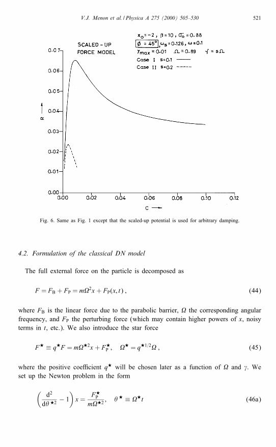
Fig. 6. Same as Fig. 1 except that the scaled-up potential is used for arbitrary damping.
4.2. Formulation of the classical DN model
The full external force on the particle is decomposed as
F = FB + FP = m2x + FP(x; t) ; (44)
where FB is the linear force due to the parabolic barrier, the corresponding angularfrequency, and FP the perturbing force (which may contain higher powers of x, noisyterms in t, etc.). We also introduce the star force
F? ≡ q?F = m?2x + F?P ; ? = q?1=2 ; (45)
where the positive coe�cient q? will be chosen later as a function of and . Weset up the Newton problem in the form
(d2
d� ?2 − 1)
x =F?P
m?2 ; � ? ≡ ?t (46a)
522 V.J. Menon et al. / Physica A 275 (2000) 505–530
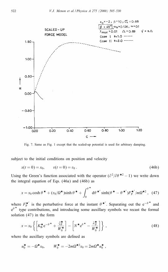
Fig. 7. Same as Fig. 1 except that the scaled-up potential is used for arbitrary damping.
subject to the initial conditions on position and velocity
x(t = 0) = x0; v(t = 0) = v0 : (46b)
Using the Green’s function associated with the operator (@2=@� ?2− 1) we write downthe integral equation of Eqs. (46a) and (46b) as
x = x0 cosh � ? + (v0=?)sinh � ? +∫ � ?
0d� ?′
sinh(� ? − � ?′)F?′P =m?2 ; (47)
where F?′P is the perturbative force at the instant � ?′
. Separating out the e−� ?and
e�?type contributions, and introducing some auxillary symbols we recast the formal
solution (47) in the form
x = x0
{[K?B e
−� ?+
�?P
W?0
]−[N?e�
? − �?P
W?0
]}; (48)
where the auxillary symbols are de�ned as
u?0 =−?x0; W?
0 =−2m?2x0 = 2m?u?0 ;
V.J. Menon et al. / Physica A 275 (2000) 505–530 523
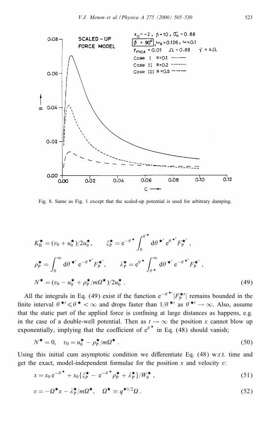
Fig. 8. Same as Fig. 1 except that the scaled-up potential is used for arbitrary damping.
K?B = (v0 + u?
0 )=2u?0 ; �?
P = e−� ?
∫ � ?
0d� ?′
e�?′F?′P ;
�?P =
∫ ∞
0d� ?′
e−� ?′F?′P ; �?
P = e� ?
∫ ∞
� ?d� ?′
e−� ?′F?′P ;
N? = (v0 − u?0 + �?
P =m?)=2u?0 : (49)
All the integrals in Eq. (49) exist if the function e−� ?′ |F?′P | remains bounded in the
�nite interval � ?′6� ? ¡∞ and drops faster than 1=� ?′ as � ?′ → ∞. Also, assumethat the static part of the applied force is con�ning at large distances as happens, e.g.in the case of a double-well potential. Then as t → ∞ the position x cannot blow upexponentially, implying that the coe�cient of e�
?in Eq. (48) should vanish;
N? = 0; v0 = u?0 − �?
P =m? : (50)
Using this initial cum asymptotic condition we di�erentiate Eq. (48) w.r.t. time andget the exact, model-independent formulae for the position x and velocity v:
x = x0 e−� ?+ x0{�?
P − e−� ?�?P + �?
P }=W?0 ; (51)
v=−?x − �?P =m?; ? ≡ q?1=2 : (52)
524 V.J. Menon et al. / Physica A 275 (2000) 505–530
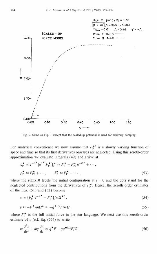
Fig. 9. Same as Fig. 1 except that the scaled-up potential is used for arbitrary damping.
For analytical convenience we now assume that F?′P is a slowly varying function of
space and time so that its �rst derivatives onwards are neglected. Using this zeroth-orderapproximation we evaluate integrals (49) and arrive at
�?P ≈ e−� ?
[e�?′F?′P ]
∞0 ≈ F?
P − F?P0 e
−� ?+ · · · ;
�?P ≈ F?
P0 + · · · ; �?P ≈ F?
P + · · · ; (53)
where the su�x 0 labels the initial con�guration at t = 0 and the dots stand for theneglected contributions from the derivatives of F?
P . Hence, the zeroth order estimatesof the Eqs. (51) and (52) become
x ≈ {F?0 e
−� ? − F?P }=m?2 ; (54)
v ≈ −F?=m? ≈ −q?1=2F=m ; (55)
where F?0 is the full initial force in the star language. We next use this zeroth-order
estimate of v (c.f. Eq. (55)) to write
md2xdt2
+ m dxdt
≈ q?F − q?1=2F= : (56)
V.J. Menon et al. / Physica A 275 (2000) 505–530 525
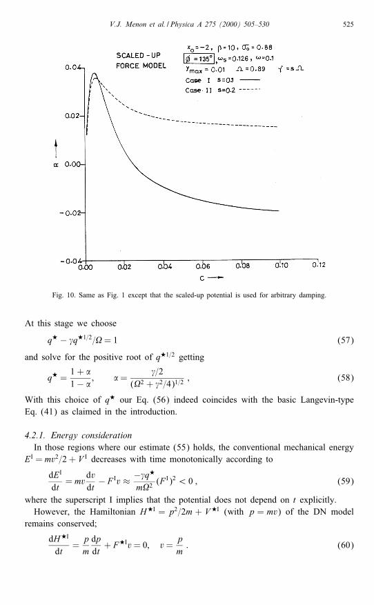
Fig. 10. Same as Fig. 1 except that the scaled-up potential is used for arbitrary damping.
At this stage we choose
q? − q?1=2= = 1 (57)
and solve for the positive root of q?1=2 getting
q? =1 + �1− �
; �= =2
(2 + 2=4)1=2; (58)
With this choice of q? our Eq. (56) indeed coincides with the basic Langevin-typeEq. (41) as claimed in the introduction.
4.2.1. Energy considerationIn those regions where our estimate (55) holds, the conventional mechanical energy
EI = mv2=2 + V I decreases with time monotonically according to
dEI
dt= mv
dvdt
− F Iv ≈ − q?
m2(F I)2¡ 0 ; (59)
where the superscript I implies that the potential does not depend on t explicitly.However, the Hamiltonian H?I = p2=2m + V?I (with p = mv) of the DN model
remains conserved;
dH?I
dt=
pmdpdt+ F?Iv= 0; v=
pm
: (60)
526 V.J. Menon et al. / Physica A 275 (2000) 505–530
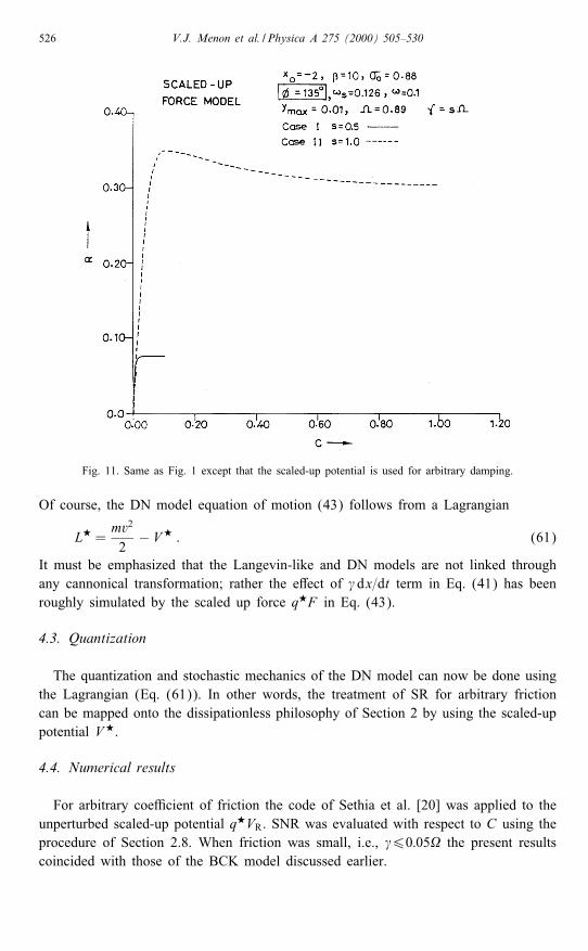
Fig. 11. Same as Fig. 1 except that the scaled-up potential is used for arbitrary damping.
Of course, the DN model equation of motion (43) follows from a Lagrangian
L? =mv2
2− V? : (61)
It must be emphasized that the Langevin-like and DN models are not linked throughany cannonical transformation; rather the e�ect of dx=dt term in Eq. (41) has beenroughly simulated by the scaled up force q?F in Eq. (43).
4.3. Quantization
The quantization and stochastic mechanics of the DN model can now be done usingthe Lagrangian (Eq. (61)). In other words, the treatment of SR for arbitrary frictioncan be mapped onto the dissipationless philosophy of Section 2 by using the scaled-uppotential V?.
4.4. Numerical results
For arbitrary coe�cient of friction the code of Sethia et al. [20] was applied to theunperturbed scaled-up potential q?VR. SNR was evaluated with respect to C using theprocedure of Section 2.8. When friction was small, i.e., 60:05 the present resultscoincided with those of the BCK model discussed earlier.
V.J. Menon et al. / Physica A 275 (2000) 505–530 527
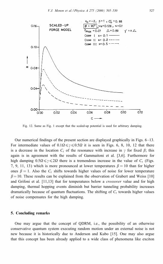
Fig. 12. Same as Fig. 1 except that the scaled-up potential is used for arbitrary damping.
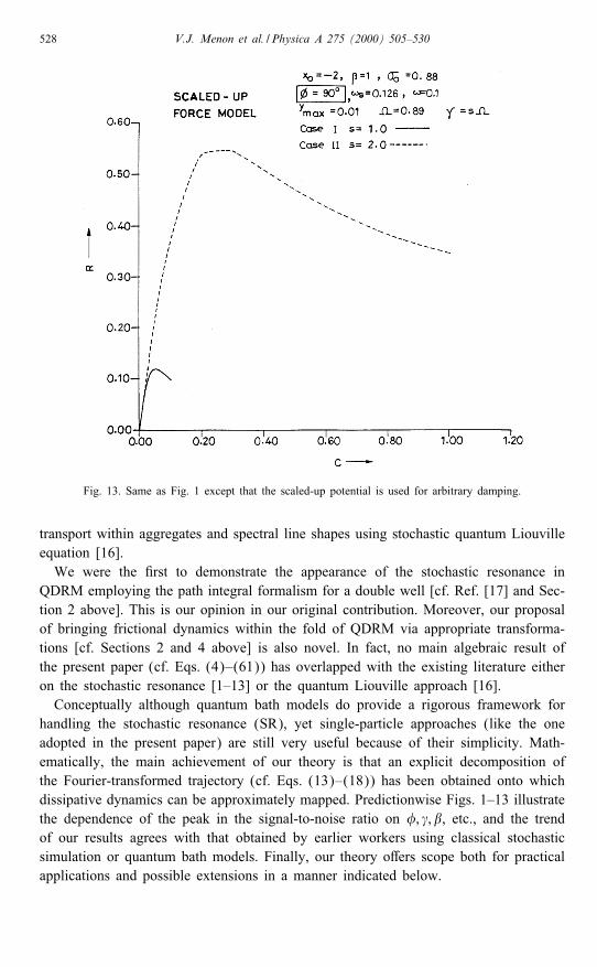
Our numerical �ndings of the present section are displayed graphically in Figs. 6–13.For intermediate values of 0:16 60:5 it is seen in Figs. 6, 8, 10, 12 that thereis a decrease in the location Cr of the resonance with increase in for �xed �; thisagain is in agreement with the results of Gammaitoni et al. [3,6]. Furthermore forhigh damping 0:56 62 there is a tremendous increase in the value of Cr (Figs.7, 9, 11, 13) which is more pronounced at lower temperatures �= 10 than for higherones � = 1. Also the Cr shifts towards higher values of noise for lower temperature�=10. These results can be explained from the observation of Grabert and Weiss [10]and Grifoni et al. [11,13] that for temperatures below a crossover value and for highdamping, thermal hopping events diminish but barrier tunneling probability increasesdramatically because of quantum uctuations. The shifting of Cr towards higher valuesof noise compensates for the high damping.
5. Concluding remarks
One may argue that the concept of QDRM, i.e., the possibility of an otherwiseconservative quantum system executing random motion under an external noise is notnew because it is historically due to Anderson and Kubo [15]. One may also arguethat this concept has been already applied to a wide class of phenomena like exciton
528 V.J. Menon et al. / Physica A 275 (2000) 505–530
Fig. 13. Same as Fig. 1 except that the scaled-up potential is used for arbitrary damping.
transport within aggregates and spectral line shapes using stochastic quantum Liouvilleequation [16].We were the �rst to demonstrate the appearance of the stochastic resonance in
QDRM employing the path integral formalism for a double well [cf. Ref. [17] and Sec-tion 2 above]. This is our opinion in our original contribution. Moreover, our proposalof bringing frictional dynamics within the fold of QDRM via appropriate transforma-tions [cf. Sections 2 and 4 above] is also novel. In fact, no main algebraic result ofthe present paper (cf. Eqs. (4)–(61)) has overlapped with the existing literature eitheron the stochastic resonance [1–13] or the quantum Liouville approach [16].Conceptually although quantum bath models do provide a rigorous framework for
handling the stochastic resonance (SR), yet single-particle approaches (like the oneadopted in the present paper) are still very useful because of their simplicity. Math-ematically, the main achievement of our theory is that an explicit decomposition ofthe Fourier-transformed trajectory (cf. Eqs. (13)–(18)) has been obtained onto whichdissipative dynamics can be approximately mapped. Predictionwise Figs. 1–13 illustratethe dependence of the peak in the signal-to-noise ratio on �; ; �, etc., and the trendof our results agrees with that obtained by earlier workers using classical stochasticsimulation or quantum bath models. Finally, our theory o�ers scope both for practicalapplications and possible extensions in a manner indicated below.
V.J. Menon et al. / Physica A 275 (2000) 505–530 529
The formulation of dissipationless SR (cf. Section 2) may be fruitfully applied toan inductance–capacitance circuit subjected to random voltage, motion of charged par-ticles in a stochastic magnetic �eld, quantum dynamics of shell-model protons in anucleus exposed to random gamma-ray pulses, charge carriers in a superconductingloop subjected to a stochastic external e.m.f, computer-simulated molecular dynamicsin which the noise is produced from a random number generator, etc. [17].The formalism of frictional SR (cf. Sections 3 and 4) may be usefully applied to
the standard bistable systems such as the electronic Schmidt trigger, bidirectional ringlaser, two-level spin–boson system, etc. [27–29]. In the end it may be pointed out thatthere is scope for re�ning the formalism still further by incorporating the e�ects ofcolored noise, nonperiodic modulation, temperature-dependent friction, etc., but theseaspects will be discussed in a future communication.
Acknowledgement
VJM thanks the UGC for �nancial support.
References
[1] R. Benzi, A. Sutera, A. Vulpiani, J. Phys. A 14 (1981) L453.[2] T. Munakata, Prog. Theor. Phys. 75 (1986) 747.[3] L. Gammaitoni, E.M. Saetta, S. Santucci, F. Marchesoni, C. Presilla, Phys. Rev. A 40 (1989) 2114.[4] B. McNamara, K. Wiesenfeld, Phys. Rev. A 39 (1989) 4854.[5] P. Jung, P. Hanggi, Phys. Rev. A 41 (1990) 2977.[6] L. Gammaitoni, F. Marchesoni, E.M. Saetta, S. Santucci, Phys. Rev. E 49 (1994) 4878.[7] D.R. Chialvo, A. Longtin, J.M. Gerking, Phys. Rev. E 55 (1997) 1798.[8] F.C. Blondeau, Phys. Rev. E 55 (1997) 2016.[9] A. Buchleitner, R.N. Mantegna, Phys. Rev. Lett. 80 (1998) 3932.[10] H. Grabert, U. Weiss, Phys. Rev. Lett. 53 (1984) 1787.[11] M. Grifoni, L. Hartmann, S. Berchtold, P. Hanggi, Phys. Rev. E 53 (1995) 5890.[12] D.O. Riele, A.K. Pattanayak, W.C. Shieve, Phys. Rev. E 51 (1995) 2925.[13] M. Grifoni, P. Hanggi, Phys. Rev. E 54 (1996) 1390.[14] R.P. Feynman, A.R. Hibbs, Quantum Mechanics and Path Integrals, McGraw-Hill, New York, 1965,
pp. 34, 342.[15] R. Kubo, M. Toda, N. Hashitsume, Statistical Physics II, Springer, Berlin, 1985, p. 266 (Chapter 2)
references.[16] K. Lindenberg, B.J. West, Nonequilibrium Statistical Mechanics of Open and Closed Systems, VCH,
New York, 1990, pp. 294, 296 (Chapters 6, 8).[17] N. Chanana, V.J. Menon, Y. Singh, Ind. J. Phys. B 71 (1997) 147.[18] S. Chandrasekhar, Rev. Mod. Phys. 15 (1943) 1 (Eq. (217)).[19] N. Chanana, V.J. Menon, Y. Singh, Phys. Rev. E 53 (1996) 5477 (Eq. (4)).[20] A. Sethia, S. Sanyal, Y. Singh, J. Chem. Phys. 93 (1990) 7268.[21] E. Kanai, Prog. Theor. Phys. 3 (1948) 440.[22] V.J. Menon, N. Chanana, Y. Singh, Prog. Theor. Phys. 98 (1997) 321.[23] W.M. Zhang, D.H. Feng, Phys. Rev. A 52 (1995) 1746.[24] A.O. Caldeira, A.J. Leggett, Physica A 121 (1983) 587.
530 V.J. Menon et al. / Physica A 275 (2000) 505–530
[25] D. Thirumalai, B.J. Berne, J. Chem. Phys. 81 (1984) 2512.[26] V.J. Menon, N. Chanana, Y. Singh, Pramana 50 (1998) 333.[27] S. Fauve, F. Heslot, Phys. Lett. A 97 (1983) 5.[28] B. McNamara, K. Wiesenfeld, R. Roy, Phys. Rev. Lett. 60 (1988) 2626.[29] E.G. Petrov, I.A. Goychuk, V. May, Phys. Rev. E 54 (1996) 4500.