arX

iv:1

207.

5863

v2 [

gr-q

c] 1

2 N

ov 2

012

Stochastic background of relic gravitons in a bouncing quantum cosmological model

Dennis Bessada1,3, Nelson Pinto-Neto2‡, Beatriz B. Siffert2,4† and Oswaldo D. Miranda3§1UNIFESP - Universidade Federal de Sao Paulo - Laboratorio de Fısica Teorica e Computacao Cientıfica,

Rua Sao Nicolau, 210, 09913-030, Diadema, SP, Brazil2ICRA - CBPF - Centro Brasileiro de Pesquisas Fısicas - Rua

Dr. Xavier Sigaud, 150, Urca, 22290-180, Rio de Janeiro, Brazil3INPE - Instituto Nacional de Pesquisas Espaciais - Av. dos Astronautas,

1758, 12227-010, Sao Jose dos Campos, SP, Brazil4Instituto de Fısica - Universidade Federal do Rio de Janeiro -

Av. Athos da Silveira Ramos 149, 21941-972, Rio de Janeiro, Brazil

The spectrum and amplitude of the stochastic background of relic gravitons produced in a bounc-ing universe is calculated. The matter content of the model consists of dust and radiation fluids, andthe bounce occurs due to quantum cosmological effects when the universe approaches the classicalsingularity in the contracting phase. The resulting amplitude is very small and it cannot be observedby any present and near future gravitational wave detector. Hence, as in the ekpyrotic model, anyobservation of these relic gravitons will rule out this type of quantum cosmological bouncing model.

PACS numbers: 98.80.Cq

I. INTRODUCTION

Bouncing cosmological models [1] are being widely in-vestigated because, besides solving the singularity prob-lem in cosmology by construction, they can also solvethe horizon and flatness puzzles, and lead to an almostscale invariant spectrum of scalar perturbations if thecontracting phase is dominated by dust at large scales[2].

One of the calculations that have been done was theevaluation of the spectral index of long wavelength ten-sor perturbations, nT , and in most of bouncing modelsthey were found to be also scale invariant. With respectto their amplitudes, specific models must be worked out.For instance, in the cyclic ekpyrotic scenario, they wereevaluated and it was shown that the amplitudes are toosmall to be detected by present gravitational wave detec-tors [3].

In this paper we will calculate the spectrum and am-plitude of relic gravitons in a different bouncing cos-mological model. It consists of a Friedmann-Lemaıtre-Robertson-Walker (FLRW) universe filled by dust andradiation, which is contracting classically. As it ap-proaches the singularity, quantum cosmological effectson the background, here described through the Wheeler-DeWitt equation interpreted along the lines of the Bohm-de Broglie quantum theory, avoids the singularity andejects the universe to the expanding phase we are nowexperiencing. Note that our bouncing model is very con-servative: there is nothing else than dust and radiation,we are working with a 3+ 1 dimensional space-time, andwe are performing a canonical quantization of the secondorder perturbed (with respect to the FLRW background)Einstein-Hilbert action of general relativity, interpretedalong the lines of a quantum theory appropriate to quan-tum cosmology, namely, one which does not need anyexternal agent to the quantum system to give a meaningto the quantum calculations.

Evolution of quantum perturbations (scalar, vectorand tensor) on these quantum backgrounds can be de-scribed by simple equations, as it was demonstrated inRefs. [4, 5]. With these equations, we were able to cal-culate the spectrum (analytically and numerically) andamplitude (numerically) of this stochastic background ofrelic gravitons. Although, the spectrum and amplitudediffer considerably from the cyclic ekpyrotic scenario, themain conclusion remains the same, namely, that the am-plitudes are too small to be detected by any present andnear future gravitational wave detectors.

The paper is divided as follows: in the next sectionwe review the main aspects of the quantum cosmologi-cal bouncing model on which the relic gravitons evolves,and we obtain the dynamical equations that the tensorperturbations which describe these relic gravitons mustobey. In section III we derive the expression for the criti-cal fraction of the relic gravitons energy density from thetensor perturbations described in section II. In sectionIV we calculate the spectrum and amplitude of this en-ergy density and the graviton strain either analytically(for the spectrum) and numerically. We end up with theconclusions.

II. THE STOCHASTIC BACKGROUND OF

RELIC GRAVITONS IN A BOUNCING

QUANTUM COSMOLOGICAL MODEL

We start reviewing the key ideas concerning tensor per-turbations in a perfect fluid quantum cosmological modelin the Bohm-de Broglie interpretation as put forward inRefs. [4, 6].

2

A. Hamiltonian formalism for tensor perturbations

We start with an Einstein-Hilbert action coupled to aperfect fluid described by the Schutz formalism [7]:

S = SGR + Sfluid = − 1

6ℓ2Pl

∫ √−gRd4x+

∫ √−gPd4x,

(1)where ℓ

Pl= (8πG

N/3)1/2 is the Planck length in natural

units (~ = c = 1), P is the perfect fluid pressure whosedensity ρ is given by the equation of state P = ωρ, withω = const.

Writing down the action of a fluid as proportional tothe pressure has also been proposed by other authors [8].All these approaches are generally covariant, but theyyield a preferred time direction, the one connected withthe surfaces of constant potential of the velocity field ofthe fluid.

Such very simple fluids can also be completely charac-terized by the k-essence lagrangian (∂µφ∂

µφ)(w+1)/(2w),where φ is a scalar field and w is a constant. This scalarfield has equation of state p = wρ. It has no potentialand a non-trivial kinetic term. The matter Hamiltonianwhich we will exhibit below can be easily obtained fromthis Lagrangian after one performs a simple canonicaltransformation.

This fluid description is suitable to describe the pri-mordial universe, when radiation dominates and all par-ticles become relativistic, if we make the choice w = 1/3.In what folows, we will directly quantize this perfect fluidLagrangian. This can be justified in physical grounds be-cause it was implementes while studying superfluids [9],and the quantum model based on this procedure turnedout to be quite accurate in describing many properties ofsuch physical systems.The metric g in Eq. (1) is decomposed into a back-

ground Friedman-Lemaıtre-Robertson-Walker (FLRW)metric and into a first-order tensor perturbation wij , andis given in the Arnowitt-Deser-Misner (ADM) formalismby

ds2 = N2 (τ) dτ2 − a2phys (τ) (γij + wij) dxidxj . (2)

The background metric γij is related to the spacelike hy-persurfaces with constant curvature K (K = 0,±1 forflat, open and closed space respectively), and lowers andraises the indices of the tensor perturbation wij , which

is transverse and traceless (i.e. , wij|j = 0 and wi

i = 0,

where the bar indicates a covariant derivative with re-spect to γ). N(τ) is the lapse function and defines thegauge, fixed once and for all.The second-order Hamiltonian for the gravitational

model described by the action (1) and metric (2) canbe written as (see Ref. [6] for further details)

H ≡ NH0

= N

−P2a

4a−Ka+ PT

a3ω

(

1 +ω

4

∫

d3xγ1/2 wijwij

)

+5P 2

a

48a

∫

d3xγ1/2 wijwij

+

∫

d3x

[

6ΠijΠij

a3γ1/2+ 2

PawijΠij

a2+ γ1/2a

(

wij|kwij|k

24+

K6wijw

ij

)]

, (3)

where the quantities Pa,Πij , PT are the momenta canon-

ically conjugate to the scale factor, the tensor perturba-tions, and to the fluid degree of freedom, respectively.These quantities have been redefined in order to be di-mensionless. For instance, the physical scale factor aphyscan be obtained from the dimensionless a present in (3)

through aphys = ℓPla/

√V , where V is the comoving vol-

ume of the background spacelike hypersurfaces. ThisHamiltonian, which is zero due to the constraint H0 ≈ 0,yields the correct Einstein equations both at zeroth andfirst order in the perturbations, as can be checked explic-itly. In order to obtain its expression, no assumption hasbeen made about the background dynamics, just Legen-dre and canonical transformations have been performed.

The fact that the momentum PT appears linearly inthe Hamiltonian suggests to consider its canonical posi-tion T as a time variable. Indeed, from the canonicaltransformation used to arrive at this expression [8], one

has that φ = T , (Lm = (∂µφ∂µφ)(w+1)/(2w)) that is, it is

just the potential of the fluid velocity, which character-izes a prefered foliation of spacetime. This time variablealways increases, as it can be checked in the contractingand expanding classical solutions, and in the Bohmianbounce solution we present below.

In the quantum regime, this Hamiltonian can be sub-stantially simplified through the implementation of thequantum canonical transformation generated by

U = exp(iGq) ≡ exp

(

i

12βaQ

)

, (4)

where βa ≡ 12

(

Paa+ aPa

)

and Q ≡∫

d3x γ1/2wijwij

are the self-adjoint operators associated with the corre-sponding classical variables, yielding, for a particular fac-tor ordering of (3) (see Section 3 in Ref. [6] for further

3

details), the following quantum Hamiltonian

H0 =

[

− 1

4aP 2a − Ka+ P

T

a3ω+

∫

d3x

(

6ΠijΠij

γ1/2a3

+1

24γ1/2awij|kw

ij|k +1

12γ1/2Kwijw

ija

)]

. (5)

Performing an inverse Legendre transform on thesecond-order piece of the Hamiltonian (5), and restoring

the constant ℓPl, we get the following Lagrangian density

L(2) =1

24ℓ2Pl

√

−(0)g[

(0)gαβwij|αwi

j|β − 2Kwijw

ji

]

,(6)

where (0)gαβ is the background piece of the full metric(2). Note that Lagrangian (6) coincides with the onederived in [10] for classical backgrounds.

B. Quantum evolution of the background and

perturbation variables

The quantization procedure of the background andtensor perturbations can be implemented by imposingH0Ψ(a, wij) = 0. The Wheeler-DeWitt equation in thiscase reads

i∂Ψ

∂T= HredΨ

≡

a3ω−1

4

∂2

∂a2−Ka3ω+1 +

∫

d3x

[

−6a3(ω−1)

γ1/2δ2

δwijδwij+ a3ω+1

(

γ1/2wij|kw

ij|k

24+ Kwijw

ij

12

)]

Ψ, (7)

where we have chosen T as the time variable, which isequivalent to impose the time gauge N = a3ω . Next, us-ing the Bohm-de Broglie interpretation of quantum me-chanics [11], making the separation ansatz for the wavefunctional Ψ[a, wij , T ] = ϕ(a, T )ψ[a, wij , T ], and follow-ing the reasoning of Ref. [12]1, we can show that Eq. (7)can be split into two, namely

i∂ϕ

∂T=a3ω−1

4

∂2ϕ

∂a2−Ka3ω+1ϕ, (8)

and

i∂ψ

∂T=

∫

d3x

[

−6a3(ω−1)

γ1/2δ2

δwijδwij

+ a3ω+1

(

γ1/2wij|kw

ij|k

24+Kwijw

ij

12

)]

ψ. (9)

Using the Bohm-de Broglie interpretation, Eq. (8) cannow be solved as in Refs. [13–15], yielding a Bohmianquantum trajectory a(T ), which in turn can be usedto simplify Eq. (9) [6]. Indeed, as one can understanda(T ) as a prescribed function of time, which implies thatψ(a, wij , T ) = ψ(a(T ), wij , T ) = ψ′(wij , T ), one can per-form the time dependent unitary transformation

U = exp

i

[∫

d3xγ1/2a′wijw

ij

2a

]

exp

i

[∫

d3x

(

wijΠij +Πijwij

2

)

ln

(√12

a

)]

, (10)

yielding the following simple form for the Schrodinger equation for the perturbations:

i∂ϕ(w, η)

∂η=

∫

d3x

− 1

2γ1/2δ2

δw2 + γ1/2[

1

2wkw

k − a′′

2aw2

]

ϕ(w, η). (11)

1 We are assuming that there is a disentangled zeroth order term in

the total wave function. It is a reasonable physical assumption as

long as the semi-classical theory of cosmological perturbations,

where the background behaves classically and perturbations are

quantum, seems to describe quite well our real universe. This

would be impossible if the wave function were completely entan-

gled. Note that there is no definite theory of initial conditions

for the wave function of the universe, hence one must rely in such

post-factum assumptions, one, namely, that our universe has a

classical limit.

4

A transformation to conformal time η, a3ω−1dT = dη, was also done, and a prime ′ denotes the derivative with respectto η (see again Ref. [6] for details).This Schrodinger equation is identical to the one used in semi-classical gravity for linear tensor perturbations,

but here it was obtained without ever using the background Einstein’s equations. Hence it can be used when thebackground is also quantized. It is important to stress that the function a(η) which is present in Eq. (11) is nolonger the classical solution for the scale factor, but the quantum Bohmian solution. This fact leads to some differentconsequences with respect to the usual semi-classical approach, as we will see.In the Heisenberg representation, the equations for the operator wij read

w′′ij + 2

a′

aw′

ij − w|kij|k + 2Kwij = 0, (12)

which corresponds to the usual equation for quantum tensor perturbations in classical backgrounds [10].We can proceed with the usual analysis, but now taking the quantum Bohmian solution a(η) coming from Eq. (8)

as the new pump field. In order to obtain these background quantum solutions, we follow the procedure discussed inRef. [4] which, for flat spatial sections (K = 0), yields the following guidance relation

da

dT= −a

(3ω−1)

2

∂S

∂a, (13)

in accordance with the classical relations da/dT = a,H = − 12a

(3ω−1)Pa and Pa = ∂S/∂a. For the wave function

Ψ(a, T ) =

[

8Tbπ (T 2 + T 2

b )

]1/4

exp

[ −4Tba3(1−ω)

9(T 2 + T 2b )(1− ω)2

]

exp

−i[

4Ta3(1−ω)

9(T 2 + T 2b )(1− ω)2

+1

2arctan

(

TbT

)

− π

4

]

, (14)

which comes from the initial normalized gaussian at T = 0

Ψ(init)(χ) =

(

8

Tbπ

)1/4

exp

(

−χ2

Tb

)

, (15)

where Tb is an arbitrary constant, the Bohmian quantumtrajectory for the scale factor is given by

a(T ) = ab

[

1 +

(

T

Tb

)2]

13(1−ω)

, (16)

where ab is the minimum value for the scale factor atthe bounce T = 0. Note that this solution has nosingularities and tends to the classical solution whenT → ±∞. The quantity Tb, which is the width of theinitial gaussian (15), yields the curvature scale at thebounce, Lbounce ≡ Tba

3wb . There is nothing, at this stage

of quantum cosmology, which may constrain its value:we have not yet a theory of initial conditions. It is a freeparameter. However, physical considerations allow us tosay that it must be greater than the Planck length butsmaller than the curvature scale when nucleosynthesistakes place, in order to not spoil its results.The tensor perturbations are quantum-mechanical op-

erators, hence it is convenient to expand them intoFourier modes and subject them to quantization rules:

wij (x) =√6ℓ

Pl

∑

λ=+,×

∫

d3k

(2π)3/2ε(λ)ij

[

w(λ)k (η) e−ik·xa

(λ)k

+ w∗(λ)k (η) eik·xa

(λ)†k

]

, (17)

where x = (η,x), ε(λ)ij = ε

(λ)ij

(

k

)

is the polarization ten-

sor for the two graviton polarization states + and × la-beled by λ, and satisfies

ε(λ)ijε(λ′)ij = 2δλλ′ . (18)

Also, w(λ)k (η) are mode functions, and a

(λ)†k

, a(λ)k

are cre-ation and annihilation operators, respectively. Such op-erators satisfy the equal-time commutation relations

[

a(λ)k, a

(λ′)†k′

]

= δλλ′δ(3) (k− k′) , (19)

[

a(λ)k, a

(λ′)k′

]

=[

a(λ)†k

, a(λ′)†k′

]

= 0, (20)

and the quantum vacuum is defined by

a(λ)k

|0〉 = 0. (21)

This vacuum initial condition was chosen because theuniverse in the contracting phase was very big, rarefiedand almost flat, where inhomogeneities are supposed tobe wiped out through dissipation, see Ref. [5] on that.This is a general assumption in bouncing models.Next, inserting the Fourier expansion into Eq. (12),

we get the mode equation

w(λ)′′k + 2

a′

aw

(λ)′k +

(

k2 + 2K)

w(λ)k = 0. (22)

5

Introducing the canonical amplitude v(λ)k as

v(λ)k ≡ aw

(λ)k , (23)

mode equation (22) becomes

v(λ)′′

k +

(

k2 + 2K − a′′

a

)

v(λ)k = 0, (24)

for each graviton polarization state. In the present work,we will only be concerned with the case K = 0, i.e., aUniverse with flat spatial sections.

III. STOCHASTIC BACKGROUND OF RELIC

GRAVITONS

In the ΛCDM model, quantum fluctuations arisingduring inflation lead to a nearly scale-invariant spectrumof density (scalar) [16] and gravitational waves (tensor)perturbations [17]. As in the case of CMB, we also expectrelic gravitons generated in this early epoch to form abackground – the stochastic background of relic gravitons(SBRG) – to be hopefully detected by the high-sensitivitygravitational waves (GW) detectors. The physical ob-servable to be measured by such GW detectors is thecritical fraction of the relic gravitons energy density ρGW

given by (see [18, 19] and references therein)

ΩGW (η) ≡ ρGW (η)

ρc, (25)

where ρc = (H/ℓPl)2 is the critical energy density. The

energy density ρGW carried by the relic gravitons is sim-ply the 0-0 component of the stress energy-momentumtensor of the tensor perturbations, that is ρGW = T 0

0,where

Tαβ ≡ − 2√

−(0)g

∂L(2)

∂(0)gαβ, (26)

and L(2) is the Lagrangian (6) for the tensor perturba-tions (recall that Lagrangian (6) holds either in classical

or quantum backgrounds). Considering only spatially-flat models (K = 0), the energy density of the relic gravi-tons can be derived by inserting (6) into (26) and takingthe 0-0 component, which yields the classical expression

ρGW =1

12ℓ2Pl

[

1

a2wij ′wij

′ − 1

2wij,µwij,µ

]

. (27)

Since tensor fluctuations generated during inflation areof quantum nature, the energy density of the relic gravi-tons becomes the expected value of the operator T 0

0 inthe vacuum state defined in (21):

ρGW ≡ 〈0|T 00|0〉. (28)

Substituting the Fourier expansion (17) into (27), and theresult into (28), we find, using the commutation relations(19,20,21), that

ρGW (η) =1

a2

∑

λ

∫

d ln kk3

4π2

[

∣

∣

∣w

(λ)′

k (η)∣

∣

∣

2

+ k2∣

∣

∣w

(λ)k (η)

∣

∣

∣

2]

. (29)

In terms of the canonical field v(λ)k introduced in (23),

expression (29) turns into

ρGW (η) =

∫

d ln k ρGW (k, η) , (30)

where we have introduced the energy density per mode

ρGW (k, η) ≡ dρGW (η)

d ln k

=k3

4π2a4

∑

λ

∣

∣

∣v(λ)′

k

∣

∣

∣

2

−H[

v(λ)k v

(λ)′∗k

+ v(λ)∗k v

(λ)′

k

]

+(

k2 +H2)

∣

∣

∣v(λ)k

∣

∣

∣

2

, (31)

where H = a′/a is the Hubble parameter in conformaltime coordinates.From (31) the energy density parameter (25) per mode

is given by

ΩGW (k, η) =ℓ2Pl

2π2a2k3

H2

∑

λ

∣

∣

∣v(λ)′

k

∣

∣

∣

2

−H[

v(λ)k v

(λ)′∗k + v

(λ)∗k v

(λ)′

k

]

+(

k2 +H2)

∣

∣

∣v(λ)k

∣

∣

∣

2

. (32)

By solving the mode equation (24) and inserting theresult into (32), we promptly determine the energy den-sity parameter per logarithmic frequency interval ν =k/(2πa), which is the physical quantity to be confrontedwith future observations.

IV. STOCHASTIC BACKGROUND OF RELIC

GRAVITONS IN A DUST-RADIATION

BOUNCING UNIVERSE

A. Scale Factor

The scale factor for the radiation dominated bouncewill be given by Eq. (16), with w = 1/3. In this case, we

6

have dT = dη so, we find

abounce(η) = ab

√

1 +

(

η

ηb

)2

, (33)

where ηb is a free parameter that determines the durationof the bouncing phase.The scale factor before and after the bounce is the

usual classical solution for a Universe filled with radiationand dust [20],

arad(η) = aeq

[

(

η

η∗

)2

∓ 2η

η∗

]

, (34)

where the minus and plus signs refers to the epochs beforeand after the bounce, respectively, aeq is the value of thescale factor at matter-radiation equality, and

η∗ = 2RH

√

2 + zeq

1 + zeq, (35)

where RH = 1/(a0H0) is the co-moving Hubble radius,a0 and H0 are the present values of the scale factor andHubble radius, respectively, and zeq ≈ 3 × 103 is thevalue of the redshift at matter-radiation equality. As thebounce should occur much before the matter-radiationequality, then ηb << η∗.The above expressions for abounce and arad can be con-

densed into

a(η) = aeq

(

η

η∗

)2

+ 2ηbη∗

√

1 +

(

η

ηb

)2

, (36)

which promptly recovers Eqs. (33) and (34) in the limitsη << η∗ and η >> ηb, respectively, and assuming thatab = 2aeqηb/η∗.With this expression for the scale factor, we are ready

to solve the mode equation, Eq. (24).

B. Mode Equation

For numerical purposes, we prefer to work with thenormalized variables

η ≡ η

2RHand n ≡ 2RHk. (37)

In terms of these variables, the mode equation for aflat Universe becomes

d2vndη2

+

[

n2 − d2a

dη21

a

]

vn = 0, (38)

where we are treating separately each possible gravitonpolarization state, so we have dropped the superscript(λ).The scale factor given in Eq. (36) becomes

a(η) = aeq

(

η

η∗

)2

+ 2ηbη∗

√

1 +

(

η

ηb

)2

, (39)

where ηb = ηb/2RH is a free parameter and

η∗ =η∗

2RH=

√

2 + zeq

1 + zeq≈ 0.018. (40)

In the original set of variables η and k, the initial con-ditions to solve the mode equation are the vacuum con-ditions to be set at ηini = −∞:

vk(ηini) =e−ikηini

√2k

, (41)

dvkdη

∣

∣

∣

∣

η=ηini

= −i√

k

2e−ikηini . (42)

Using the new variables η and n, the initial conditionsto solve Eq. (38) for one of the two polarization modesare

vn(ηini) =

√

RH

ne−inηini , (43)

dvndη

∣

∣

∣

∣

η=ηini

= −i√

nRH e−inηini . (44)

We have checked that we can, in this case, numericallyconsider −∞ as any value of ηini < −3.The present value of η, η0, is obtained by solving Eq.

(39) for η = η0, which results in

η0 = −√

2− zeq + 2 + zeq

1 + zeq≈ 0.982. (45)

We can constrain the free parameter ηb by demandingthat the end of the bouncing phase happens between thePlanck time (z ≈ 1032 and the beginning of nucleosyn-thesis (z ≈ 1010), which results in

10−31 . ηb . 10−9. (46)

We have solved Eq. (38) from ηini to η0 for four dif-ferent values of ηb in this range: 10−30, 10−24, 10−18 and10−12.In terms of the new variables η and n, the expression

for the density parameter in Eq. (32), for one of the twopossible polarizations, can be rewritten as

7

ΩGW (n, η) =ℓ2Pl

2π2a2n3

32R5HH2

∣

∣

∣

∣

dvndη

∣

∣

∣

∣

2

− 2RHH×

×[

vndv∗ndη

+ v∗ndvndη

]

+(

n2 + 4R2HH2

)

|vn|2

.(47)

For η = η0, this expression reduces to

ΩGW (n, η0) =l2p

64 π2n3a0H

30

∣

∣

∣

∣

dvndη

∣

∣

∣

∣

2

− 2

[

vndv∗ndη

+

+ v∗ndvndη

]

+ (n2 + 4)|vn|2 ∣

∣

∣

∣

η=η0

.(48)

C. Analytical Results

One can anticipate the spectral behavior of the abovequantities through some analytical reasonings. Note firstthat the spectral index of tensor perturbations at themoment they get smaller than the curvature scale in theexpanding phase of the above quantum bouncing modelswas calculated in Ref. [4], and it reads

nT =12w

1 + 3w, (49)

where w is the equation of state parameter of the fluidwhich dominates the cosmic evolution when the mode isgetting bigger than the curvature scale of the Universe inthe contracting phase. When the fluid is dust, nT = 0,when it is radiation, nT = 2.The power spectrum is

P ∝ n3|µn|2 ≡ (∆hn)2 ∝ nnT , (50)

where ∆hn is the strain of the gravitational wave withwavenumber n. Hence, one can obtain the spectra ofthe strain at the moment ηc of curvature scale cross-ing at dust domination and radiation domination fromEq. (49), and they are ∆hn(ηc) ∝ n0 and ∆hn(ηc) ∝ n,respectively.However, we need the strain today, ∆hn(η0). Note

that the curvature scale is given by lc ≡ (a3/a′′)1/2

(which is equal to the Hubble radius in the case of aperfect fluid dominated classical model), and it is compa-rable to the physical wavelength of the mode k = n/RH ,lphys = a/k, when k2 = a′′/a. Hence, for lphys < lc, ork2 > a′′/a, vk oscillates (see the mode equation (24)for K = 0). Therefore, as vk = aµk, one has that|µk|(η0)a(η0) = |µk|(ηc)a(ηc) after curvature scale cross-ing at the expanding phase. Note that a(ηc) as a functionof k can be obtained through

lphys(ηc) = a(ηc)/k = lc(ηc) ∝ RH(ηc) ∝ t(ηc) ∝ a3/2(ηc)(51)

when ηc is in the dust dominated era, and

lphys(ηc) = a(ηc)/k = lc(ηc) ∝ RH(ηc) ∝ t(ηc) ∝ a2(ηc)(52)

when ηc is in the radiation dominated era. Hence onegets that a(ηc) ∝ k−2 and a(ηc) ∝ k−1 for dust and radi-ation dominated eras, respectively. Therefore, in termsof the frequency f = k/(2πa0) = nH0/(4π), the transferfunction for the strain,

∆hf (η0) = Tf∆hf (ηc), (53)

which is the same as the one for |µf |, see Eq. (50), reads

Tf ∝(

H0

f

)2(

1 +f

feq

)

, (54)

where feq = Heqaeq/a0 ≈ 10−16 Hz and H0 ≈ 10−18 Hz.Finally, the potential V (η) = (d2a/dη2)/a of Eq. (38)

derived from Eq. (39) reads

V (η) =

2

[

1η∗

+η2b

(η2b+η2)

3/2

]

η2

η∗

+ 2√

η2b + η2, (55)

and it has a maximum value at η = 0, Vmax ≈ η−2b . We

see therefore that modes with n > 1/ηb do not feel thepotential at any time, for they correspond to wavelengthsmuch smaller than the maximum curvature scale of themodel. Hence, they are always oscillating with spectrumgiven by the initial vacuum state,

vn(η) =e−inη

√2n

, (56)

and there is no graviton creation above these frequencies.Therefore, we make a cutoff at the point n > 1/ηb, sothat there is no zero-point contributions to the energydensity, and the vacuum spectrum ΩGW is clearly finite.Actually, it is important to stress that such zero-pointcontribution would affect only the high frequency sectorof our results.From Eq. (50), one then infers that the strain ∆hn has

spectrum n for n > 1/ηb, independently of η. As thebounce itself has a duration much smaller then the clas-sical dust-radiation evolution, almost all modes that donot enter the curvature scale after the beginning of clas-sical radiation domination in the expanding phase havethe above spectrum.Noting that our model is symmetric with respect to

the bounce, implying that wavelengths which leave thecurvature scale before the bounce at some fluid domi-nation era enter the curvature scale after the bounce atthe same fluid domination, we can summarize the resultsconcerning the spectrum of the strain in the followingway:

8

i) H0 ≈ 10−18Hz < f < 10−16Hz ≈ feq;∆hf (η0) ∝ f−2f0 = f−2.ii) feq ≈ 10−16Hz < f < fmax = H0/ηb;

∆hf (η0) ∝ f−1f = f0.iii) fmax = H0/ηb < f ; ∆hf (η0) ∝ f .From the above spectrum, one can easily obtain the

spectrum for the energy density parameter of gravita-tional waves from the relation

ΩGW (f, η0) ∝ f2[∆hf (η0)]2. (57)

These results are confirmed by the numerical calcula-tion we show in the sequel.

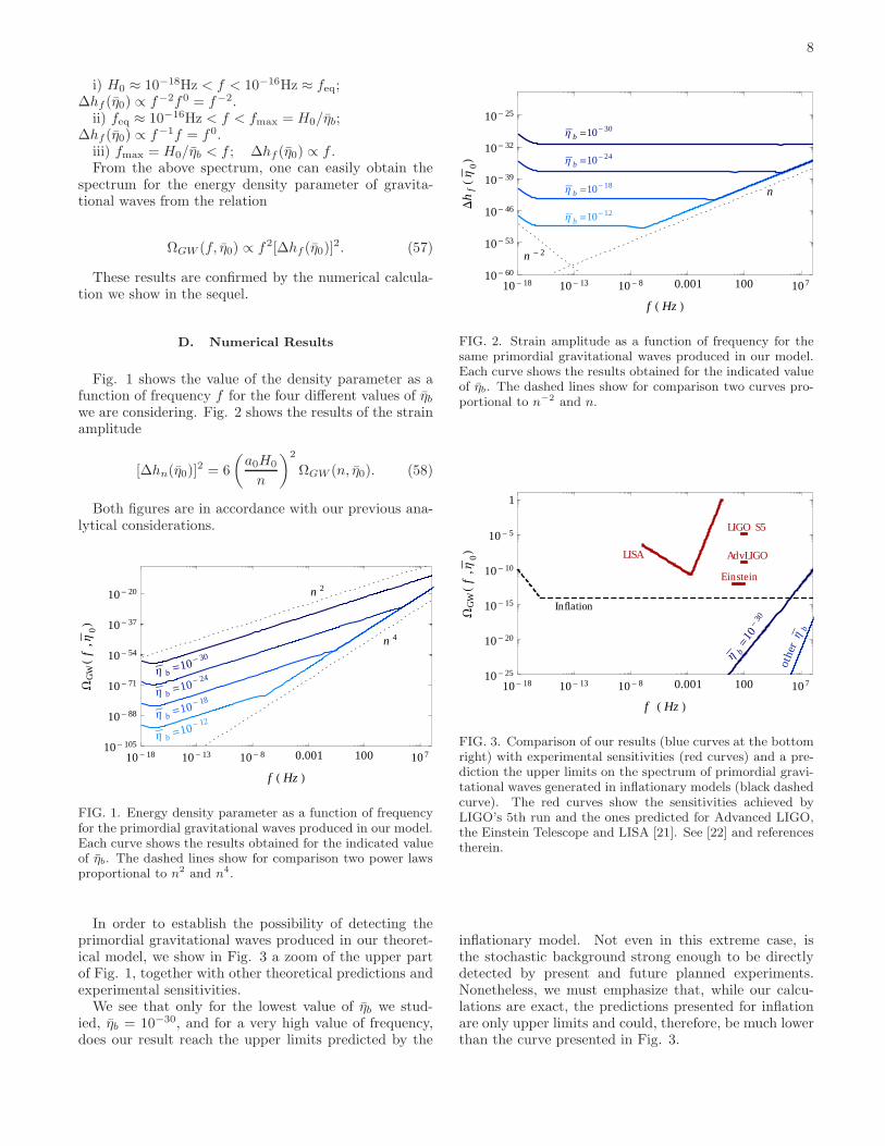
D. Numerical Results

Fig. 1 shows the value of the density parameter as afunction of frequency f for the four different values of ηbwe are considering. Fig. 2 shows the results of the strainamplitude

[∆hn(η0)]2 = 6

(

a0H0

n

)2

ΩGW (n, η0). (58)

Both figures are in accordance with our previous ana-lytical considerations.

10- 18 10- 13 10- 8 0.001 100 10 710- 105

10- 88

10- 71

10- 54

10- 37

10- 20

f H Hz L

WG

WH

f,Η

0L

Η b=10-

18

Η b=10-

12

Η b=10-

24Η b=10-

30

n 4

n 2

FIG. 1. Energy density parameter as a function of frequencyfor the primordial gravitational waves produced in our model.Each curve shows the results obtained for the indicated valueof ηb. The dashed lines show for comparison two power lawsproportional to n

2 and n4.

In order to establish the possibility of detecting theprimordial gravitational waves produced in our theoret-ical model, we show in Fig. 3 a zoom of the upper partof Fig. 1, together with other theoretical predictions andexperimental sensitivities.We see that only for the lowest value of ηb we stud-

ied, ηb = 10−30, and for a very high value of frequency,does our result reach the upper limits predicted by the

10- 18 10- 13 10- 8 0.001 100 10 710- 60

10- 53

10- 46

10- 39

10- 32

10- 25

f H Hz L

Dh

fHΗ

0L

Η b =10- 18

Η b =10- 12

Η b =10- 24

Η b =10- 30

n

n - 2

FIG. 2. Strain amplitude as a function of frequency for thesame primordial gravitational waves produced in our model.Each curve shows the results obtained for the indicated valueof ηb. The dashed lines show for comparison two curves pro-portional to n

−2 and n.

10- 18 10- 13 10- 8 0.001 100 10 710- 25

10- 20

10- 15

10- 10

10- 5

1

f H Hz L

WG

WH

f,Η

0L

Inflation

LIGO S5

AdvLIGOLISA

Einstein

othe

rΗ

b

Η b=

10-

30

FIG. 3. Comparison of our results (blue curves at the bottomright) with experimental sensitivities (red curves) and a pre-diction the upper limits on the spectrum of primordial gravi-tational waves generated in inflationary models (black dashedcurve). The red curves show the sensitivities achieved byLIGO’s 5th run and the ones predicted for Advanced LIGO,the Einstein Telescope and LISA [21]. See [22] and referencestherein.

inflationary model. Not even in this extreme case, isthe stochastic background strong enough to be directlydetected by present and future planned experiments.Nonetheless, we must emphasize that, while our calcu-lations are exact, the predictions presented for inflationare only upper limits and could, therefore, be much lowerthan the curve presented in Fig. 3.

9

V. CONCLUSIONS

In this paper we have calculated the amplitude andspectrum of energy density and strain of relic gravitonsin a quantum bouncing cosmological model. The strainspectrum of this quantum bouncing model is differentfrom the cyclic and inflationary scenarios. While thesetwo models have spectra ≈ k−2,≈ k−1 at dust domina-tion, and ≈ k−1,≈ k0 at radiation domination, respec-tively, our model have spectra ≈ k−2 and ≈ k0 at thesame eras.One possible different scenario in which the power of

relic gravitons could be enhanced could be obtained byadding to the matter content of the model some amountof stiff matter, which has primordial spectral index nT =2. This will be the subject of future investigations.As a final point, as in the cyclic ekpyrotic model, the

resulting amplitude is too small to be detected by anygravitational wave detector. In particular, the sensitiv-ity of the future third generation of gravitational wavedetectors, as for example the Einstein Telescope, could

reach ΩGW ∼ 10−12 at the frequency range 10 − 100Hzto an observation time of ∼ 5 years and with a signal-to-noise ratio (S/N) ∼ 3. Therefore, any detection ofrelic gravitons, in this frequency range, will rule out thistype of quantum bouncing model as a viable cosmologicalmodel of the primordial universe.

ACKNOWLEDGMENTS

DB thanks the Brazilian agency FAPESP, grant2009/15612-6 for financial support, and ICRA-CBPF forits kind hospitality. BBS would like to acknowledgethe financial support of CAPES under grant numberCAPES-PNPD 2940/2011 and to thank CNPq for the2010-2011 PCI fellowship. NPN would like to thankCNPq for financial support. ODM would like to thankthe Brazilian agency CNPq for partial financial support(grant 300713/2009-6). The authors also thank SandroVitenti for his kind help with numerical methods.

[1] M. Novello and S. E. Perez Bergliaffa, Phys. Rep. 463,127 (2008).

[2] R. Brandenberger and F. Finelli, J. High Energy Phys.11 (2001) 056; P. Peter and N. Pinto-Neto, Phys. Rev. D66, 063509 (2002); F. Finelli, JCAP 0310, 011(2003);V. Bozza and G. Veneziano, Phys. Lett. B 625, 177(2005); V. Bozza and G. Veneziano, JCAP 09, 007(2005); F. Finelli and R. Brandenberger, Phys. Rev.D 65 (2002) 103522; S. Tsujikawa, R. Brandenbergerand F. Finelli, Phys. Rev. D 66, 083513 (2002); P. Pe-ter, N. Pinto-Neto and D. A. Gonzalez, JCAP 0312,003 (2003); J. Martin, P. Peter, Phys. Rev. Lett 92,061301 (2004); J Martin, P Peter, N Pinto-Neto andD. J. Schwarz, Phys. Rev. D 65, 123513 (2002); J Mar-tin, P Peter, N Pinto-Neto and D. J. Schwarz, Phys.Rev. D 67, 028301 (2003); C. Cartier, R. Durrer andE. J. Copeland, Phys. Rev. D. 67, 103517 (2003);L. E. Allen and D. Wands, Phys. Rev. D 70, 063515(2004); T. J. Battefeld, and G. Geshnizjani, Phys. Rev.D 73, 064013 (2006); A Cardoso and D Wands, Phys.Rev. D 77, 123538 (2008); Y Cai, T Qiu, R Branden-berger, Y Piao and X Zhang, J. Cosmol. Astropart. Phys.03 (2008) 013.

[3] L. A. Boyle, P. J. Steinhardt and N. Turok, Phys. Rev.D 69, 127302 (2004).

[4] P. Peter, E. J. C. Pinho and N. Pinto-Neto, Phys. Rev.D 73, 104017 (2006) [arXiv:gr-qc/0605060].

[5] E. J. C. Pinho and N. Pinto-Neto, Phys. Rev. D 76

023506 (2007); P. Peter, E. J. C. Pinho, and N. Pinto-Neto, Phys. Rev. D 75 023516 (2007).

[6] P. Peter, E. Pinho, N. Pinto-Neto, JCAP 0507, 014(2005). [hep-th/0509232].

[7] B. F. Schutz, Jr., Phys. Rev. D2 2762 (1970); Phys. Rev.D4, 3559 (1971).

[8] V. G. Lapchinskii, V. A. Rubakov, Theor. Math. Phys.33, 1076 (1977); V. Fock, Theory of Space, Time and

Gravitation (Pergamon, London, (1959).[9] I. M. Khalatnikov, An Introduction to the Theory of

Super-fluidity (W. A. Benjamin, New York, 1965).[10] V. F. Mukhanov, H. A. Feldman, and R. H. Branden-

berger, Phys. Rep. 215, 203 (1992).[11] See e.g. P. Holland, The Quantum Theory of Motion,

Cambridge University Press (Cambridge, UK, 1993) andreferences therein.

[12] F. T. Falciano and N. Pinto-Neto, Phys. Rev. D 79,023507 (2009) and arXiv:0810.3542v2 [gr-qc].

[13] J. Acacio de Barros, N. Pinto-Neto, and M. A. Sagioro-Leal, Phys. Lett. A 241, 229 (1998).

[14] R. Colistete Jr., J. C. Fabris, and N. Pinto-Neto, Phys.Rev. D62, 083507 (2000).

[15] F.G. Alvarenga, J.C. Fabris, N.A. Lemos and G.A. Mon-erat, Gen.Rel.Grav. 34, 651 (2002).

[16] A. Guth, S. Y. Pi, Phys. Rev. Lett.49, 1110(1982); A. A. Starobinsky, Phys. Lett. B 117, 175(1982); S. Hawking, Phys. Lett. B 115, 295 (1982);J. M. Bardeen, P. J. Steinhardt, and M. S. Turner, Phys.Rev. D28, 679 (1983).

[17] V. A. Rubakov, M. V. Sazhin, A. V. Veryaskin, Phys.Lett. B115, 189-192 (1982); R. Fabbri, M. d. Pol-lock, Phys. Lett. B125, 445-448 (1983); L. F. Ab-bott, M. B. Wise, Nucl. Phys. B244, 541-548 (1984);B. Allen, Phys. Rev. D37, 2078 (1988); L. P. Grishchuk,Phys. Rev. Lett. 70, 2371-2374 (1993), [gr-qc/9304001];M. S. Turner, M. J. White, J. E. Lidsey, Phys. Rev. D48,4613-4622 (1993), [astro-ph/9306029].

[18] M. Giovannini, PMC Phys. A4, 1 (2010).[arXiv:0901.3026 [astro-ph.CO]].

[19] M. Maggiore, Phys. Rept. 331, 283-367 (2000).[gr-qc/9909001].

[20] V. Mukhanov, “Physical foundations of cosmology,”Cambridge University Press (2005).

[21] [LISA is not a project anymore. A new mission called

10

European New Gravitational Wave Observatory (NGO)has been derived from the previous LISA proposal. Thisnew mission whose informal name is “eLISA” will surveyfor the first time the low-frequency gravitational waveband (about 0.1mHz to 1Hz)]; Amaro-Seoane P. et al.,

2012, Class. Quantum Grav., 29, 124016 - eLISA/NGO.[22] The LIGO Scientific Collaboration and The Virgo

Collaboration, Nature 460, 990-994 (2009); B.Sathyaprakash et al., “Scientific Objectives of EinsteinTelescope”, Class. Quantum Grav. 29, 124013, 2012.