gravitational clustering of relic neutrinos and implications for their detection

arX

iv:h

ep-p

h/04

0824

1v2

24

Nov

200

4

DESY 04-147

Gravitational clustering of relic neutrinos and

implications for their detection

Andreas Ringwald and Yvonne Y. Y. Wong

Deutsches Elektronen-Synchrotron DESY, D-22607 Hamburg, Germany

Abstract. We study the gravitational clustering of big bang relic neutrinos onto

existing cold dark matter (CDM) and baryonic structures within the flat ΛCDM model,

using both numerical simulations and a semi-analytical linear technique, with the aim

of understanding the neutrinos’ clustering properties for direct detection purposes. In

a comparative analysis, we find that the linear technique systematically underestimates

the amount of clustering for a wide range of CDM halo and neutrino masses.

This invalidates earlier claims of the technique’s applicability. We then compute

the approximate phase space distribution of relic neutrinos in our neighbourhood

at Earth, and estimate the large scale neutrino density contrasts within the local

Greisen–Zatsepin–Kuzmin zone. With these findings, we discuss the implications

of gravitational neutrino clustering for scattering-based detection methods, ranging

from flux detection via Cavendish-type torsion balances, to target detection using

accelerator beams and cosmic rays. For emission spectroscopy via resonant annihilation

of extremely energetic cosmic neutrinos on the relic neutrino background, we give new

estimates for the expected enhancement in the event rates in the direction of the Virgo

cluster.

E-mail: [email protected], [email protected]

http://arXiv.org/abs/hep-ph/0408241v2

Gravitational clustering of relic neutrinos and implications for their detection 2

1. Introduction

The standard big bang theory predicts the existence of 1087 neutrinos per flavour in

the visible universe (e.g., [1]). This is an enormous abundance unrivalled by any other

known form of matter, falling second only to the cosmic microwave background (CMB)

photon. Yet, unlike the CMB photon which boasts its first (serendipitous) detection

in the 1960s and which has since been observed and its properties measured to a high

degree of accuracy in a series of airborne/satellite and ground based experiments, the

relic neutrino continues to be elusive in the laboratory. The chief reason for this is

of course the feebleness of the weak interaction. The smallness of the neutrino mass

also makes momentum-transfer-based detection methods highly impractical. At present,

the only evidence for the relic neutrino comes from inferences from other cosmological

measurements, such as big bang nucleosynthesis (BBN) and CMB together with large

scale structure (LSS) data (e.g., [2]). Nevertheless, it is difficult to accept that these

neutrinos will never be detected in a more direct way.

In order to design possible direct, scattering-based detection methods, a precise

knowledge of the phase space distribution of relic neutrinos is indispensable. In this

connection, it is important to note that an oscillation interpretation of the atmospheric

and solar neutrino data (e.g., [3]) implies that at least two of the neutrino mass

eigenstates are nonrelativistic today. These neutrinos are subject to gravitational

clustering on existing cold dark matter (CDM) and baryonic structures, possibly causing

the local neutrino number density to depart from the standard value of nν = nν ≃56 cm−3, and the momentum distribution to deviate from the relativistic Fermi–Dirac

function.

In this paper, we develop a method that will allow us to predict the phase space

distribution of relic neutrinos in our local neighbourhood at Earth (∼ 8 kpc from the

Galactic Centre), as well as in outer space. The method systematically takes into

account gravitational clustering of relic neutrinos on scales below ∼ 5 Mpc, and can be

applied to the complete range of experimentally and observationally consistent neutrino

masses. With these predictions, we determine the precise implications of relic neutrino

clustering for future direct search experiments. To this end, we note that in earlier

studies of relic neutrino direct detection, the neutrino number density in our local

neighbourhood is either assumed to be unrealistically large, or simply left as a free

parameter (e.g., [4, 5, 6]). With the emergence of the concordance flat ΛCDM model

as the cosmological model of choice, today we are in a position to compute the relic

neutrino phase space distribution within a well defined cosmological framework, and

to contemplate again the prospects for their direct detection in a definitive way. Our

studies here will also be useful for such investigations as relic neutrino absorption [7, 8, 9]

and emission [10, 11, 12, 13, 14] spectroscopy.

The standard procedure for any gravitational clustering investigation is to solve

the (1 + 3 + 3)-dimensional Vlasov, or collisionless Boltzmann, equation using N -body

techniques (e.g., [15, 16, 17, 18]). However, these techniques are computationally very


expensive and necessarily come with limited resolutions. In the context of the cold+hot

dark matter (CHDM) model, earlier N -body studies involving neutrinos probe their

kinematic effects on structure formation from cluster and galaxy abundances on large

scales (e.g., [19, 20, 21, 22]), to halo properties on small scales [23]. While the CHDM

model has fallen out of favour in recent years (see, however, [24]), it is instructive to

note that the halo simulation of [23] has a formal resolution of only ∼ 100 kpc. This is

clearly inadequate for our considerations, where the scale of interest is of order 1 kpc.

In the context of the flat ΛCDM model, Singh and Ma (hereafter, SM) presented a

novel approximate method to probe the accretion of neutrinos onto CDM halos at scales

below ∼ 50 kpc [25]. The salient feature of this study is their use of parametric halo

density profiles from high resolution, pure ΛCDM simulations as an external input, while

the neutrino component is treated as a small perturbation whose clustering depends

on the CDM halo profile, but is too small to affect it in return. Implementation of

this approximation requires the neutrino mass density ρν to be much smaller than its

CDM counterpart ρm. On cosmological scales, we know now from LSS data that the

ratio ρν/ρm = Ων/Ωm is at most ∼ 0.2 [2]. On cluster/galactic scales, neutrino free-

streaming ensures that ρν/ρm always remains smaller than its cosmological counterpart

[23]. Thus the approximation scheme, so far, is sound. Furthermore, in order to track

the neutrino density fluctuations in the most effortless way, SM employed the linearised

Vlasov equation instead of its full version. Unfortunately, linear methods are known to

break down when the density fluctuations reach the order of unity. Indeed, in their two

trial runs with CHDM parameters, the linear results of SM compare favourably with

N -body results of [23] in the outer part of the halo, where the neutrino overdensity is

relatively low. The denser inner parts (<∼ 1 Mpc), however, show marked disagreement.

This discrepancy renders SM’s claim that their complete prescription is able to probe

neutrino clustering on sub-galactic scales doubtful.

In the present investigation, we adopt one of the more attractive features of SM’s

study, namely, the use of parametric halo profiles as an external input. However, we

improve upon their analysis by solving the Vlasov equation in its (almost) full glory

utilising a restricted, N -1-body (pronounced: EN-ONE-BODY) method based on the

following observation: In the limit ρν ≪ ρm and the CDM contribution dominates the

total gravitational potential, not only will the CDM halo be gravitationally blind to the

neutrinos, the neutrinos themselves will also have negligible gravitational interaction

with each other. This allows us to track them one particle at a time in N independent

simulations, instead of following N particles simultaneously in one single run, as in

a conventional N -body study. An obvious advantage of our N -1-body technique is

that it requires virtually no computing power when compared with a full scale N -body

simulation with the same, large N (>∼ 106). It is also less time-consuming since we

have done away with the need for a gravity solver (the core of all N -body techniques).

In addition, restricted methods such as ours do not suffer from spurious two body

relaxation, and hence do not require the introduction of an artificial softening length that

is mandatory in conventional N -body studies. Lastly, we note that restricted methods


have been used extensively in the studies of galaxy interactions (e.g., [26]), and, when

properly motivated, should not be seen as inferior to full scale N -body techniques.

As a closing remark, let us stress again that our purpose here is not to investigate

the effects of neutrino mass on cosmology, but rather to address some simple questions

such as how many relic neutrinos can we realistically expect to find in this very space

we occupy, what kind of energies do they have, where in the universe can we expect to

find the highest concentration of relic neutrinos, etc., given what we know today about

cosmology. In this regard, the analysis we present here is most exhaustive.

The paper is organised as follows. We begin in section 2 with an assessment of

the current observational constraints on the relic neutrino background. In section 3,

we introduce the Vlasov equation which is used to track the phase space distribution

of the neutrinos. Section 4 contains a brief discussion of the halo density profiles to be

employed in our calculations. In section 5, we solve the Vlasov equation for the halo

models using our improved N -1-body method for a variety of halo and neutrino masses.

In section 6, we compute for the same halo models and neutrino masses the neutrino

overdensities using the linear method of SM and examine its validity. Section 7 deals

exclusively with relic neutrinos in the Milky Way, and in particular their phase space

distribution in our immediate vicinity. We discuss in section 8 the implications of our

findings for scattering-based detection methods, and we conclude in section 9.

2. Observational constraints on the relic neutrino background

Taking as our basis (i) the flat ΛCDM model with (Ωm,0,ΩΛ,0) ∼ (0.3, 0.7) and Hubble

parameter h ∼ 0.7, (ii) neutrino mass splittings inferred from the solar and atmospheric

data, (∆m2sun,∆m

2atm) ∼ (10−5, 10−3) eV2, and (iii) the invisible Z decay width from

LEP which constrains the number of SU(2) doublet neutrinos to three [27], a minimal

theory of neutrino clustering is fixed only by the absolute masses of the neutrinos mν .

The current laboratory limit from tritium β decay experiments is mν < 2.2 eV (2σ)

[28, 29], and should improve to ∼ 0.35 eV with the upcoming KATRIN experiment [30].

Cosmology also provides a constraint on mν . For three degenerate species, an upper

bound of∑mν < 1.7 eV (2σ) [31, 32, 33] has been inferred from a combined analysis

of the CMB anisotropy from WMAP [34] and galaxy clustering from SDSS (SDSS-gal)

[35] (or from 2dFGRS [36]), together with an HST prior on the Hubble parameter [37].

(Reference [32] uses also SNIa [38]).‡ Adding to the fit galaxy bias [39] and Lyα forest

analyses can tighten the constraint to∑mν < 0.42 eV [40] (see also [41, 42, 43, 44]),

although the robustness of these additional inputs is still contentious. Weak lensing of

galaxies [45] or of the CMB [46] will provide an alternative probe for the cosmological

implications of massive neutrinos.

While constraints from cosmology are interesting in their own right, they are also

highly model dependent, and degeneracies abound. For instance, if tensors and running

‡ The mass splittings inferred from the solar and atmospheric neutrino oscillation experiments imply

that the three mass eigenstates are quasi-degenerate when mν ≫√

∆m2atm.


of the scalar spectral index are allowed, the last∑mν bound relaxes to 0.66 eV [40].

Another possibility is an interplay between mν and Nν , where Nν is the effective number

of thermalised fermionic degrees of freedom present in the radiation-dominated era, such

that increasing Nν actually weakens the bound on mν [33]. For example, a Nν = 6

model receives a CMB+LSS+priors constraint of (i)∑mν < 2.7 eV, if all six particles

are equally massive, (ii)∑mν < 2.1 eV, if three are massive and the others exactly

massless, and (iii)∑mν < 4.13 eV, if only one is massive [47]. Currently, 1.4 ≤ Nν ≤ 6.8

is allowed by CMB+LSS+priors [33, 42, 48, 49, 50]. Future CMB experiments such as

Planck will be sensitive to ∆Nν ∼ 0.2 [51, 52]

Lastly, we note that BBN prefers 1.84 ≤ Nν ≤ 4.54 (2σ), in the absence of a νechemical potential ζνe [53] (see also [50, 54]). Allowing for a nonzero ζνe weakens the

bounds to 1.3 ≤ Nν ≤ 7.1 for −0.1 ≤ ζνe ≤ 0.3 [55]. There is no lack of candidates in the

literature for these extra Nν − 3 degrees of freedom. We shall not list them here. What

is certain, however, is that they cannot take the form of very large chemical potentials

in the νµ,τ sectors, since large neutrino mixing inferred from oscillation experiments

ensures that ζνe ∼ ζνµ ∼ ζντ < 0.3, too small to be a significant source of Nν [56, 57, 58].

In the present analysis, we assume the neutrinos to constitute exactly three

thermalised fermionic degrees of freedom, and adopt a conservative mass bound of

mν <∼ 0.6 eV, (2.1)

corresponding to the Nν = 3 constraint from the WMAP+SDSS galaxy cluster analysis

[31]. Alternatively, (2.1) may be interpreted as a restrictive bound for models with

extra, non-neutrino relativistic particles (Nν > 3), or with a significant running spectral

index, as discussed earlier.

3. Vlasov equation

A system consisting of several types of weakly interacting, self-gravitating particles [e.g.,

CDM plus neutrinos] may be modelled as a multi-component collisionless gas whose

phase space distributions fi(x,p, τ) obey the Vlasov equation (e.g., [18, 59]),

DfiDτ

≡ ∂fi∂τ

+ x · ∂fi∂x

+ p · ∂fi∂p

= 0. (3.1)

The single-particle phase density fi(x,p, τ) is defined so that dNi = fi d3x d3p is the

number of i particles in an infinitesimal phase space volume element. The variables

x = r/a(t), p = amix, dτ = dt/a(t), (3.2)

are the comoving distance, its associated conjugate momentum, and the conformal time

respectively, with a as the scale factor and mi the mass of the ith particle species.

All temporal and spatial derivatives are taken with respect to comoving coordinates,

i.e., ˙ ≡ ∂/∂τ , ∇ ≡ ∂/∂x.§ In the nonrelativistic, Newtonian limit, equation (3.1) is

§ Unless otherwise indicated, we shall be using comoving spatial and temporal quantities throughout

the present work. Masses and densities, however, are always physical.


equivalent to

∂fi∂τ

+p

ami· ∂fi∂x

− ami∇φ · ∂fi∂p

= 0, (3.3)

with the Poisson equation

∇2φ = 4πGa2∑

i

ρi(τ)δi(x, τ), (3.4)

δi(x, τ) ≡ρi(x, τ)

ρi(τ)− 1, ρi(x, τ) =

mi

a3

∫d3p fi(x,p, τ), (3.5)

relating the peculiar gravitational potential φ(x, τ) to the density fluctuations δi(x, τ)

with respect to the physical mean ρi(τ).

The Vlasov equation expresses conservation of phase space density fi along each

characteristic x(τ),p(τ) given by

dx

dτ=

p

ami,

dp

dτ= −ami∇φ. (3.6)

The complete set of characteristics coming through every point in phase space is thus

exactly equivalent to equation (3.1). It is generally not possible to follow the whole set

of characteristics, but the evolution of the system can still be traced, to some extent, if

we follow a sufficiently large but still manageable sample selected from the initial phase

space distribution. This forms the basis of particle-based solution methods.

4. Halo density profiles and other preliminary concerns

A “first principles” approach to neutrino clustering requires the simultaneous solution

of the Vlasov equation (3.1) [or, equivalently, the equations for the characteristics (3.6)]

for both the CDM and the neutrino components. In our treatment, however, we assume

only the CDM component ρm contributes to φ in the Poisson equation (3.4), and ρm to be

completely specified by halo density profiles from high resolution ΛCDM simulations.

We provide in this section further justifications for this approach, as well as a brief

discussion on the properties of the halo density profiles to be used in our analysis.

It is well known that after they decouple from the cosmic plasma at T ∼ 1 MeV,

light neutrinos (mν ≪ 1 keV) have too much thermal velocity to cluster on small

scales via gravitational instability in the early stages of structure formation. Accretion

onto CDM protoclusters becomes possible only after the neutrino velocity has dropped

below the velocity dispersion of the protoclusters. The mean velocity of the unperturbed

neutrino distribution has a time dependence of

〈v〉 ≃ 1.6 × 102 (1 + z)(

eV

mν

)km s−1, (4.1)

where z is the redshift. A typical galaxy cluster has a velocity dispersion of about

1000 km s−1 today; a typical galaxy, about 200 km s−1. Thus, for sub-eV neutrinos,

clustering on small scales can only have been a z <∼ 2 event.


On the other hand, based on a systematic N -body study of halo formation in

a variety of hierarchical clustering cosmologies, Navarro, Frenk and White (hereafter,

NFW) argued in 1996 that density profiles of CDM halos conform to a universal shape,

generally independently of the halo mass, the cosmological parameters and the initial

conditions [60, 61]. This so-called NFW profile has a two-parameter functional form

ρhalo(r) =ρs

(r/rs)(1 + r/rs)2, (4.2)

where rs is a characteristic inner radius, and ρs = 4ρ(rs) a corresponding inner density.

These parameters rs and ρs are determined by the halo’s virial mass Mvir and a

dimensionless concentration parameter c defined as

c ≡ rvir

rs, (4.3)

where rvir is the virial radius, within which lies Mvir of matter with an average density

equal to ∆vir times the mean matter density ρm at that redshift, i.e.,

Mvir ≡4π

3∆virρma

3r3vir =

4π

3∆virρm,0r

3vir

= 4πρsa3r3s

[ln(1 + c) − c

1 + c

], (4.4)

where ρm,0 is the present day mean matter density. The factor ∆vir is usually taken to

be the overdensity predicted by the dissipationless spherical top-hat collapse model δTH,

which takes on a value of ∼ 178 for an Einstein–de Sitter cosmology, while the currently

favoured ΛCDM model has δTH ≃ 337 at z = 0.‖Within this framework, any halo density profile is completely specified by its virial

mass and concentration via equations (4.2) to (4.4). Indeed, the NFW profile in its two-

parameter form generally gives, for quiet isolated halos, a fit accurate to ∼ 10% in the

range of radii r = 0.01 → 1 rvir [18]. Furthermore, NFW argued for a tight correlation

between Mvir and c, such that the mass distribution within a halo is effectively fixed

by the halo’s virial mass alone. Later studies support, to some extent, this conclusion

(e.g., [62, 63, 64]); halo concentration correlates with its mass, albeit with a significant

scatter. The analysis of [64] of ∼ 5000 halos in the mass range 1011 → 1014M⊙ reveals

a trend (at z = 0) described by

c(z = 0) ≃ 9

(Mvir

1.5 × 1013h−1M⊙

)−0.13

, (4.5)

with a 1σ spread about the median of ∆(log c) = 0.18 for fixed Mvir. In addition, for a

fixed virial mass, the median concentration parameter exhibits a redshift dependence of

c(z) ≃ c(z = 0)

1 + z(4.6)

between z = 0 and z = 4.

In their analysis, SM interpreted the set of equations (4.2) to (4.6) as a complete

description of an individual halo’s evolution in time. While we do not completely

‖ In the original work of NFW [60, 61], rvir is taken to be the radius r200, within which the average

density is 200 times the critical density of the universe, irrespective of the cosmological model in hand.


disagree with this interpretation, it should be remembered that the relations (4.5) and

(4.6) refer only to the behaviour of the statistical mean for fixed virial masses, and do

not actually describe how individual halos accrete mass over time. A better motivation

for the equations’ use comes from the observation that the physical densities of the inner

regions of individual isolated halos tend to remain very stable over time (z ∼ 2 → 0)

[65]. This behaviour, as it turns out, can be more or less reproduced by equations (4.2)

to (4.6), if we interpret Mvir as the halo’s virial mass today. Merging subhalos tend

to affect the main halo’s density profile only in its outer region. Therefore, provided

that neutrino clustering becomes important only after z ∼ 2 and the halos have had no

major mergers since then, we are justified to either use these equations here, or simply

model the CDM halo as a static object in physical coordinates, as a first approximation.

Finally, we note that there exists in the literature a number of other halo profiles

(e.g., [66, 67]), which, in some cases, provide better fits to simulations than does the

NFW profile (4.2). However, these profiles generally differ from (4.2) by less than 10%

[18] so we do not consider them in our study.

5. N-1-body simulations

Using the NFW halo density profile (4.2) as an input, we find solutions to the Vlasov

equation in the limit ρν ≪ ρm by solving the equations for the characteristics (3.6). We

discuss below the basic set-up. Technical details can be found in the Appendix.

5.1. Basic set-up and assumptions

We model the CDM distribution as follows. We assume that throughout space is a

uniform distribution of CDM. On top of it, sits a spherical NFW halo at the origin.

In order that the halo overdensity merges smoothly into the background density, we

extend the NFW profile to beyond the virial radius. Furthermore, for convenience, we

treat the NFW profile as a perturbation ρm(τ)δm(x, τ), rather than a physical density.

This simplification should make very little difference to the final results, since the halo

density is always much larger than the background density. The halo’s properties and

its evolution in time are contained in the set of equations (4.2) to (4.6). For the factor

∆vir, we take a time-independent value ∆vir = 200, following [68] and SM. We choose

this somewhat uncommon definition so as to facilitate direct comparisons between the

results of SM and those of the present study. However, since the choice of ∆vir affects the

profile only through rs [see equation (A.10) in the Appendix], we can see immediately

that using instead the more common ∆vir = δTH, where

δTH ≃ 18π2 + 82y − 39y2

Ωm(z), y = Ωm(z) − 1, (5.1)

with Ωm(z) = Ωm,0/(Ωm,0 + ΩΛ,0a3) [69], will make little difference to the outcome.

A more important issue is the role played by other CDM structures (i.e., other

halos and voids) that should realistically be in the surroundings. In our present scheme,


these have all been lumped into one uniform background so as to preserve the spherical

symmetry of the problem. In reality, these structures will induce tidal forces and distort

the symmetry. However, we expect tidal forces to be important only for clustering in

the outer part of the halo where the gravitational potential is low and several halos may

compete for the same neutrinos. Clustering in the deep potential well of the inner part,

on the other hand, should not be seriously affected.

For the neutrinos, we take the initial distribution to be the homogeneous and

isotropic Fermi–Dirac distribution with no chemical potential,

f0(p) =1

1 + exp(p/Tν,0), (5.2)

where Tν,0 = 1.676 × 10−4 eV is the present day neutrino temperature. In principle,

the chemical potential need not be exactly zero. In fact, a positive chemical potential

ζν should improve, to some extent, the clustering of neutrinos (as opposed to anti-

neutrinos) by providing more low velocity specimens that cluster more efficiently than do

their high velocity counterparts. However, this enhancement is necessarily accompanied

by a suppression of clustering in the anti-neutrino sector, for which a negative ζν = −ζνtends to deplete the low velocity states. Currently, the upper bound on ζν is 0.3, too

small to warrant a detailed investigation into a possible “clustering asymmetry”.

We simulate initial momentum values in the range 0.01 ≤ p/Tν,0 ≤ 13, which

accounts for more than 99.9% of the distribution (5.2). The initial spatial positions of

the neutrinos range from r = 0, to as far as it takes for the fastest particles to land

within a distance of 10 h−1Mpc from the halo centre at z = 0. We consider a sample

of three neutrino masses, mν = 0.15, 0.3, 0.6 eV, consistent with the bound (2.1), and

a range of halo viral masses, Mvir = 1012M⊙ → 1015M⊙, corresponding to halos of the

galaxy to the galaxy cluster variety. All simulations model a flat ΛCDM cosmology,

with the parameters (Ωm,0,ΩΛ,0, h) = (0.3, 0.7, 0.7)

The initial spatial and momentum distribution is divided into small chunks that

move under the external potential of the CDM halo, but independently of each other. A

low resolution run is first carried out for each set of mν ,Mvir. All chunks that end up

at z = 0 inside a sphere of radius 10 h−1Mpc centred on the halo are traced back to their

origin, subdivided into smaller chunks, and then re-simulated. The process is repeated

until the inner ∼ 10 h−1kpc is resolved. The initial redshift is taken to be z = 3.

This should be sufficient, since clustering is not expected to be fully under way until

z ∼ 2. The final neutrino density distribution is constructed from the set of discrete

particles via a kernel density estimation method [65, 70] outlined in the Appendix, with

a maximum smoothing length of ∼ 2 h−1kpc in the inner ∼ 50 h−1kpc of the halo.

5.2. Results and discussions

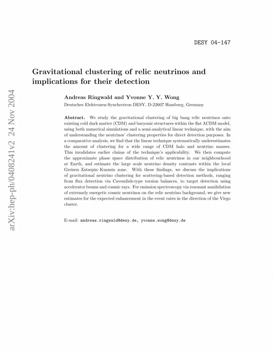
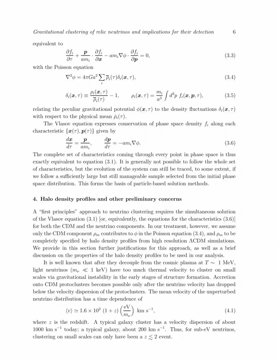
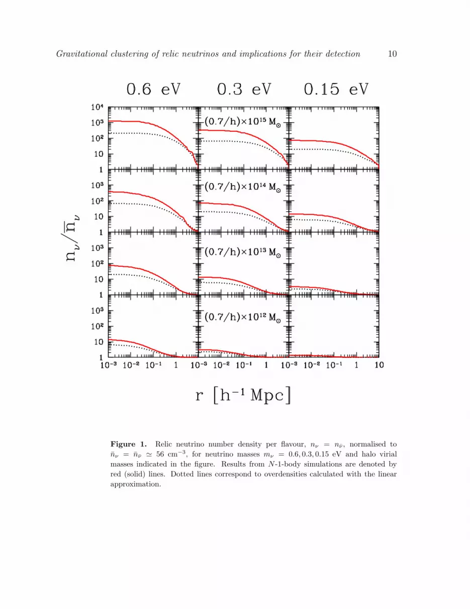
The basic results of our N -1-body simulations are presented in Figure 1, which shows

the neutrino overdensities nν/nν for various sets of mν ,Mvir. A companion figure,


Figure 1. Relic neutrino number density per flavour, nν = nν , normalised to

nν = nν ≃ 56 cm−3, for neutrino masses mν = 0.6, 0.3, 0.15 eV and halo virial

masses indicated in the figure. Results from N -1-body simulations are denoted by

red (solid) lines. Dotted lines correspond to overdensities calculated with the linear

approximation.


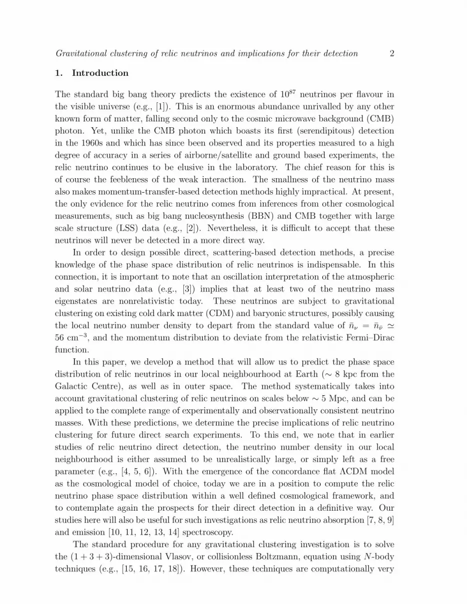
Figure 2. Mass density ratio ρν/ρm normalised to the background mean ρν/ρm

obtained from N -1-body simulations for various neutrino and halo masses indicated in

the figure.

Figure 2, shows the same results expressed in terms of the mass density ratio ρν/ρmnormalised to the background mean ρν/ρm.

The essential features of the curves in Figures 1 and 2 can be understood in terms

of neutrino free-streaming, which causes the nν/nν curves to flatten out at small radii,

and the mass density ratio ρν/ρm to drop substantially below the background mean.

(The latter feature also provides a justification for our N -1-body method.) Both nν/nνand ρν/ρm approach their respective cosmic mean of 1 and ρν/ρm at large radii. Similar

behaviours have also been observed in the CHDM simulations of reference [23].


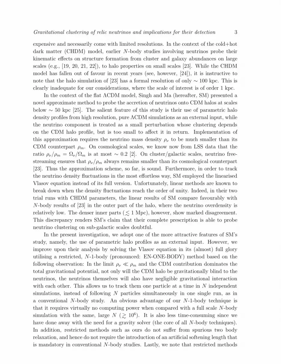
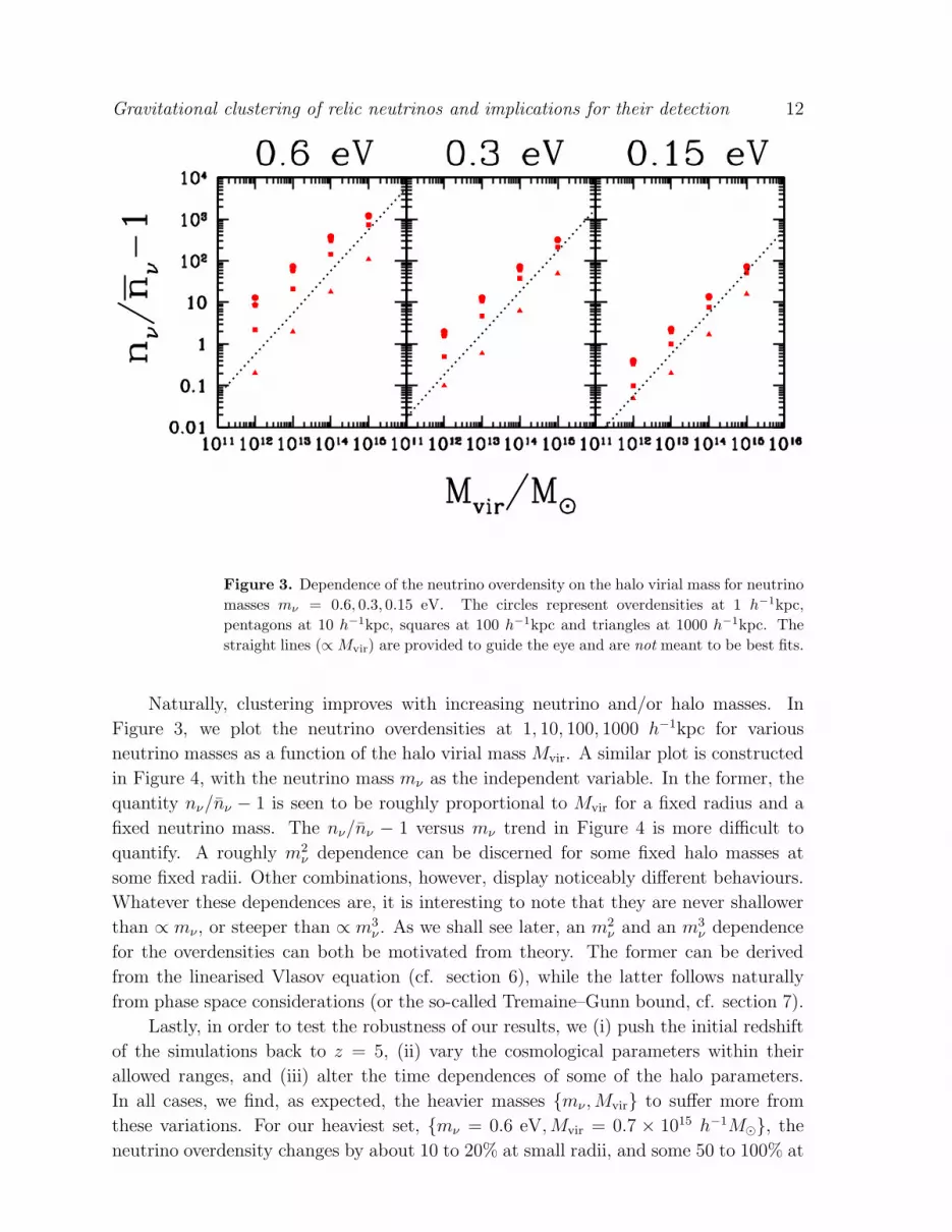
Figure 3. Dependence of the neutrino overdensity on the halo virial mass for neutrino

masses mν = 0.6, 0.3, 0.15 eV. The circles represent overdensities at 1 h−1kpc,

pentagons at 10 h−1kpc, squares at 100 h−1kpc and triangles at 1000 h−1kpc. The

straight lines (∝ Mvir) are provided to guide the eye and are not meant to be best fits.

Naturally, clustering improves with increasing neutrino and/or halo masses. In

Figure 3, we plot the neutrino overdensities at 1, 10, 100, 1000 h−1kpc for various

neutrino masses as a function of the halo virial mass Mvir. A similar plot is constructed

in Figure 4, with the neutrino mass mν as the independent variable. In the former, the

quantity nν/nν − 1 is seen to be roughly proportional to Mvir for a fixed radius and a

fixed neutrino mass. The nν/nν − 1 versus mν trend in Figure 4 is more difficult to

quantify. A roughly m2ν dependence can be discerned for some fixed halo masses at

some fixed radii. Other combinations, however, display noticeably different behaviours.

Whatever these dependences are, it is interesting to note that they are never shallower

than ∝ mν , or steeper than ∝ m3ν . As we shall see later, an m2

ν and an m3ν dependence

for the overdensities can both be motivated from theory. The former can be derived

from the linearised Vlasov equation (cf. section 6), while the latter follows naturally

from phase space considerations (or the so-called Tremaine–Gunn bound, cf. section 7).

Lastly, in order to test the robustness of our results, we (i) push the initial redshift

of the simulations back to z = 5, (ii) vary the cosmological parameters within their

allowed ranges, and (iii) alter the time dependences of some of the halo parameters.

In all cases, we find, as expected, the heavier masses mν ,Mvir to suffer more from

these variations. For our heaviest set, mν = 0.6 eV,Mvir = 0.7 × 1015 h−1M⊙, the

neutrino overdensity changes by about 10 to 20% at small radii, and some 50 to 100% at


Figure 4. Dependence of the neutrino overdensity on the neutrino mass for various

halo masses indicated on the plots. The circles represent overdensities at 1 h−1kpc,

pentagons at 10 h−1kpc, squares at 100 h−1kpc and triangles at 1000 h−1kpc. The

solid lines correspond to an m2ν dependence, dashed lines an mν dependence, and

dotted lines an m3ν dependence. These lines are provided to guide the eye and are not

meant to be best fits.


r >∼ 5 h−1Mpc. The gap narrows with smaller neutrino and halo masses. For galaxy size

halos (Mvir ∼ 1012M⊙), the density variations with respect to (i), (ii) and (iii) are no

more than ∼ 10% everywhere. Thus our simulation results are generally quite robust.

6. Linear approximation

The linear approximation is often used in the literature to find approximate solutions

to the Vlasov equation. In the nonrelativistic limit, the pioneering work of Gilbert [71]

has, over the years, been applied to the study of the pure hot dark matter (HDM)

model [72], as well as in the analysis of HDM accretion onto nonadiabatic seeds such

as cosmic strings [73, 74, 75] and onto CDM halos [25]. The procedure consists of first

switching to a new time variable s ≡ ∫a−1dτ =

∫a−2dt, and then Fourier transforming

the x-dependent functions,

f(k,p, s) ≡ F [f(x,p, s)], φ(k, s) ≡ F [φ(x, s)], (6.1)

to obtain a new differential equation in Fourier space,

∂f

∂s+ik · pmν

f − imνa2(k φ ⋆∇pf) = 0, (6.2)

where k φ⋆∇pf ≡ ∫d3k′ k′ φ(k′)·∇pf(k−k′) is the convolution product. The equation

is said to be linearised when one makes the replacement

∇pf(k) → ∇pf0(p)δ(k), (6.3)

where δ(k) is the Dirac delta function, so that the convolution product becomes a

simple scalar product kφ · ∇pf0. Replacement (6.3) is valid as long as the condition

|∇p(f − f0)| ≪ |∇pf0| holds. In practice, however, the quantity ∇pf is somewhat

cumbersome to compute, so the “rule of thumb” regarding the linear approximation

is to abandon it as soon as the spatial density fluctuation δν(x, s), defined in (3.5),

exceeds order unity, as emphasised in [59, 74]. Nonetheless, the linear theory has been

time and again used beyond this putative limit. We shall also apply it to our case, to

gain physical insight as well as to see how it compares with N -1-body simulations.

Equation (6.2) together with the replacement (6.3) has a very simple solution,

f(k,p, s) = f(k,p, si)e−ik·u(s−si)

+ imν k · ∇pf0

∫ s

si

ds′a2(s)φ(k, s′)e−ik·u(s−s′), (6.4)

where u = p/mν , si is some initial time, and we take the initial phase space distribution

to be isotropic and homogeneous in space, i.e., f(k,p, si) = δ(k)f0(p). The neutrino

number density per Fourier mode relative to the mean density is obtained by integrating

(6.4) over momenta p,

nν(k, s)

nν(s)=a−3

∫d3p f(k,p, s)

a−3∫d3p f0(p)

≡ 1

nν,0

∫d3p f(k,p, s)

= δ(k) − k2∫ s

si

ds′a2(s′)φ(k, s′)(s− s′)F

[k(s− s′)

mν

], (6.5)


Table 1. Some distribution functions f0(p) and their corresponding F (q) [equation

(6.6)] that have appeared in the literature. The series solution for F (q) for the

relativistic Fermi–Dirac (FD) function was first derived in [74]. A Maxwell–Boltzmann

(MB) type distribution was adopted in [73]. The last family of distributions,

characterised by F (q)’s exponential form, appears in [59] and [76].

Distribution f0(p) F (q)

Relativistic FD [1 + exp(p/Tν,0)]−1 4

3ζ(3)

∑∞n=1(−1)n+1n(n2 + q2T 2

ν,0)−2

MB exp(−p/Tν,0) (1 + q2T 2ν,0)

−2

γ distributionnν,0

π2(γTν,0)3(1 + p2/γ2T 2

ν,0)−2 exp(−γqTν,0)

with

F (q) ≡ 1

nν,0

∫d3p e−ip·qf0(p). (6.6)

The correct form for f0(p) should be the relativistic Fermi–Dirac function (5.2), which

gives for F (q) a series representation [74]

F (q) =4

3ζ(3)

∞∑

n=1

(−1)n+1 n

(n2 + q2T 2ν,0)

2, (6.7)

where ζ(3) ≃ 1.202 is the Riemann zeta function. However, in order to simplify

calculations and/or to gain physical insight, other forms of f0(p) have also appeared

in the literature. Some are listed in Table 1, along with their corresponding F (q).

The solution to the Poisson equation (3.4) in Fourier space is

φ(k, s) = −4πGa2ρm(s)δm(k, s)

k2= −4πGρm,0δm(k, s)

ak2. (6.8)

Substituting this into (6.5) and using the definition δν(k, s) ≡ nν(k, s)/nν(s)− δ(k), we

obtain for the neutrino density fluctuations

δν(k, s) ≃ 4πGρm,0

∫ s

si

ds′a(s′)δm(k, s′)(s− s′)F

[k(s− s′)

mν

]. (6.9)

This is the “master equation” for the linear approach. We solve equation (6.9)

numerically for a variety of neutrino and halo masses. The results are presented in

Figure 1, alongside their N -1-body counterparts.

6.1. Further approximations and analytical insights

Before comparing the two approaches, let us first study the linear approximation for its

own sake. Consider the master equation (6.9). In the limit F (q) grows much faster than

a(s) and δm(k, s), i.e.,

kTν,0mν

≫ 1

a

da

ds+

1

δm

dδmds

, (6.10)


equation (6.9) may be solved by asymptotic expansion. The resulting approximate

solution looks somewhat messy at first sight,

δν(k, s) ≃ 4πGρm,0

(mν

kTν,0

)22

3ζ(3)[ln(2)a(s)δm(k, s) −

a(si)δm(k, si)∞∑

n=1

(−1)n+1 n

n2 +k2T 2

ν,0

m2ν

(s− si)2], (6.11)

but may be rendered into a physically transparent form if we first cross out the second

term, which is well justified since the initial a and δm should always be much smaller

than the final ones, and then rewrite the expression as

δν(k, s) ≃k2

fs(s)

k2δm(k, s). (6.12)

Here, kfs is but the free-streaming wave vector, defined as

kfs(s) ≡√√√√4πGa(s)ρm,0

c2ν,0=

√√√√4πGa2(s)ρm(s)

c2ν(s)

≃ 1.5√a(s)Ωm,0

(mν

eV

)h Mpc−1, (6.13)

and we identify

cν(s) ≡Tν,0

mνa(s)

√√√√ 3ζ(3)

2 ln(2)≡ cν,0a(s)

≃ 81

a(s)

(eV

mν

)km s−1 (6.14)

as the neutrino’s characteristic thermal speed.

The functional form of equation (6.12) already tells us something very interesting;

large Fourier modes in the neutrino density fluctuations are suppressed by a factor

proportional to k−2 relative to their CDM counterparts. This is clearly a manifestation

of free-streaming, which is responsible for inhibiting the growth of structures on scales

below λfs ≡ 2π/kfs. Furthermore, δν has an m2ν dependence through kfs, meaning that,

at small scales, a neutrino twice as heavy as another is able to cluster four times more

efficiently. This m2ν dependence is reflected, approximately, by both our linear and

N -1-body results in Figure 1, and is particularly pronounced at small radii.

That equation (6.12) is a solution of (6.9) is contingent upon the satisfaction of

the condition (6.10), which requires, for a fixed neutrino mass, k to be larger than

some nominal kmin determined by the rates of change of the scale factor a and of the

CDM perturbations δm(k, s). The rate of change of a is a simple and well defined

function of the cosmological model. The growth rate of δm(k, s), on the other hand, is

usually more complicated. However, because our halos are practically static in physical

coordinates, this rate (in comoving Fourier space) can only be at most of the order

of the universal expansion rate (which comes in through the conversion factor a when


we switch the halo profile from physical to comoving coordinates). Thus the condition

(6.10) is roughly equivalent to

k ≫ kmin(s) ∼mν

Tν,0a2H(s) ≃ 2

√aΩm,0 + a4ΩΛ,0

(mν

eV

)h Mpc−1, (6.15)

where H(s) is the Hubble expansion parameter at time s. Since kmin ∼ kfs at most

times, we see that equation (6.12) is indeed applicable to all k modes larger than the

free-streaming wave vector kfs.

Unfortunately, the opposite k ≪ kfs limit has no simple approximate solution

because of the complicated dependence of the scale factor a on the new time variable s.

However, we find the following formula to give a decent fit to the solution of (6.9) for a

wide range of k,

δν(k, s) ≃k2

fs

(kfs/Γ + k)2δm(k, s) ≡ K(k−1

fs k, s)δm(k, s), (6.16)

with

Γ2 ≡ 4πGρm,0

δm(k, s)

∫ s

si

ds′a(s′)δm(k, s′)(s− s′)

∣∣∣∣∣k→0

. (6.17)

Typically, Γ ∼ 1, such that for k ≪ kfs, the growth of δν approximately matches that

of δm. Therefore, equation (6.16) is roughly equivalent to

ρν(x) ∼ k3fsK(kfsx) ⋆ ρm(x), (6.18)

in real space, with K(x) ≡ F−1[K(k)] acting like a normalised filter function with

window width k−1fs , that gently smears out the neutrino density contrasts on scales

below ∼ k−1fs relative to their CDM counterparts. We shall be using equation (6.18)

again in section 8.2.

6.2. Comparison with N-1-body results: when and how the linear theory fails

Comparing the linear results from this section with N -1-body simulations from section 5,

it is immediately clear in Figure 1 that the former systematically underestimates the

neutrino overdensities over the whole range of neutrino and halo masses considered

in this study. The discrepancy is most prominent in the dense, inner regions

(r <∼ 1 h−1Mpc), and worsens as we increase (i) the neutrino mass mν , and (ii) the

halo mass Mvir. The worst case corresponds to when both mν and Mvir are large; the

case of mν = 0.6 eV,Mvir = 0.7×1015 h−1M⊙, for example, sees the N -1-body and the

linear overdensities differ by a factor of about six. For smaller neutrino and halo masses,

concordance between the two approaches improves as we move to larger radii. Indeed,

for mν = 0.15 eV,Mvir = 0.7 × 1012 h−1M⊙, complete agreement is seen throughout

the region of interest. Upon closer inspection, one finds that the linear theory ceases

to be a faithful approximation once the neutrino overdensity reaches a value of about

three or four. This is of course fully consistent with the standard lore that perturbative

methods fail once the perturbations exceed unity and nonlinear effects set in.


Can the linear approximation be salvaged? Yes, provided we impose a great deal

of smoothing. In the case of mν = 0.6 eV,Mvir = 0.7 × 1015 h−1M⊙, for example,

the overdensities computed from the two different approaches can be reconciled with

each other if we smooth them both over a scale of roughly 5 h−1Mpc. Such a large

smoothing length will render the linear method completely useless for the study of

neutrino clustering on sub-galactic scales (unless of course the neutrino mass is so small

that the overdensity does not exceed unity by much anyway). But the method can

still be useful for obtaining quick estimates of nν/nν on larger scales for absorption and

emission spectroscopy calculations (cf. section 8.2).

Finally, we note that the neutrino overdensities in Figure 2 of SM are at odds

with our linear results in Figure 1. This discrepancy cannot be ameliorated by simply

supposing that SM have normalised their neutrino densities for three flavours to the

one flavour average nν = nν ≃ 56 cm−3, since this normalisation will render some of

their results—specifically, where nν/nν < 3—unphysical. Only a normalisation to three

flavours can give these results a physical meaning, but at the expense of incompatibility

with our Figure 1, as well as with SM’s own Figure 3. We therefore conclude that SM’s

results as presented in their Figure 2 are erroneous.

7. Relic neutrinos in the Milky Way

In this section, we consider relic neutrino clustering in the Milky Way. We compute

explicitly the number of neutrinos and their distribution in momentum space in our

local neighbourhood at Earth (r⊕ ∼ 8 kpc from the Galactic Centre). This information

is essential for any direct search experiment.

7.1. Background, basic set-up and assumptions

We perform this calculation using the N -1-body method of section 5, but with a few

modifications to the external potential. Firstly, we note that the central region of the

Milky Way (<∼ 10 kpc) is dominated by baryonic matter in the form of a disk, a bulge,

and possibly a rapidly rotating bar [77]. Each of these components has its own distinct

density profile. Furthermore, in the standard theory of hierarchical galaxy formation,

baryons and dark matter are initially well mixed, and collapse together to form halos via

gravitational instability. Galactic structures arise when the baryons cool and fall out of

the original halo towards the centre [78]. As the baryons condense, their gravitational

forces tend to pull the dark matter inward, thereby distorting the inner ∼ 10 kpc of

the original halo profile (e.g., [79, 80, 81, 82]). This kind of modification to the mass

distribution is important for us at r⊕. Fortunately for our calculation, gravitating

neutrinos do not distinguish between halo and baryons. Therefore, it suffices to use

simply the total mass distribution inferred from observational data (e.g., rotation curves,

satellite kinematics, etc.), without any detailed modelling of the individual components.

What is still missing, however, is the redshift dependence of the mass distribution.


Unfortunately, we have not been able to find in the literature any simple parametric form

for this dependence. However, mass modelling of the Milky Way [83, 84] suggests that

certain observationally acceptable bulge+disk+halo models are indeed consistent with

the aforementioned theory of baryonic compression, and can be traced back to halos

originally of the NFW form by supposing that the system has undergone a phase of

adiabatic contraction [79]. Thus, for our investigation, it is probably fair to think of the

NFW profile as the initial mass distribution, and the evolution as a smooth transition

from this initial distribution to the present day one.

Instead of modelling this transition, however, our strategy here is to conduct two

series of simulations, one for the present day mass distribution of the Milky Way

(MWnow) which we assume to be static, and one for the NFW halo (NFWhalo) that

would have been there, had baryon compression not taken place. The real neutrino

overdensity should then lie somewhere between these two extremes.

For the NFWhalo run, we use the parameters Mvir = 1×1012M⊙ and c = 12. These

numbers are taken from the paper of Klypin, Zhao and Somerville (hereafter, KZS) [84],

from their “favoured” mass model of the Milky Way. Note that we are not using the

c-Mvir relation (4.5), which, as we discussed before, is only a statistical trend. However,

the concentration parameter c should still carry a redshift dependence a la equation

(4.6), in order to reproduce the correct time dependence of the density profile.

For MWnow, we adopt the total mass distribution (halo+disk+bulge) presented in

Figure 3 of KZS, and fit it approximately to a power law from r = 0 to 20 kpc,

Mfit(r, z = 0) = 2 × 1011

(r

20 kpc

)1.19367

M⊙, (7.1)

where M(r) means the total mass contained within a radius r. We assume this fit to hold

for the region inside a physical radius of 20 kpc at all times, i.e., Mfit(r, z) = Mfit(ar, z =

0). The region outside of this 20 kpc sphere is not affected by baryonic compression

according to the KZS mass model (cf. their Figure 7) so we adopt the original NFW

density profile outwardly from 20 kpc. Thus, schematically, we have

M(r, r < r0) = Mfit(r),

M(r, r ≥ r0) = MNFW(r) −MNFW(r0) +Mfit(r0), (7.2)

where r0 = 20 a−1 kpc, MNFW(r) is the mass contained in an NFW halo at radius r [or

Mhalo(r) in equation (A.7)], and Mfit(r0) ≃ 2 ×MNFW(r0) for the parameters used in

this analysis.

7.2. Results and discussions

Our Milky Way simulation results for four neutrino mass mν = 0.15, 0.3, 0.45, 0.6 eV are

displayed in Figure 5. The shaded region in each plot corresponds to a possible range

of overdensities at z = 0. At first glance, it may seem unphysical that the apparently

static MWnow potential (in physical coordinates) should capture so many neutrinos. To

resolve this “paradox”, one must remember that neutrino clustering is studied in the


Figure 5. Relic neutrino number density per flavour, nν = nν , in the Milky Way for

various neutrino masses. All curves are normalised to nν = nν ≃ 56 cm−3. The top

curve in each plot corresponds to the MWnow run, and the bottom to the NFWhalo

run. The enclosed region represents a possible range of overdensities at z = 0.

context of an expanding universe; the (unbound) neutrino thermal velocity decreases

with time [equation (4.1)], thus causing them to be more readily captured. Equivalently,

in comoving coordinates, it is easy to see that while the neutrino conjugate momentum

(3.2) does not redshift, the MWnow potential well shrinks in size and deepens with time.

In each scenario we studied, the final momentum distribution at r⊕ is almost

isotropic, with a zero mean radial velocity 〈vr〉, and second velocity moments that

satisfy approximately the relation 2〈v2r〉 = 〈v2

T 〉 (cf. Table 2). For this reason, we plot


Table 2. Velocity moments at r⊕ for various neutrino masses in the MWnow and

NFWhalo runs (see text for definitions). The first column shows the overdensities

nν/nν . The second, third and fourth columns show the mean radial, transverse and

absolute velocities in terms of the dimensionless quantities 〈yr〉, 〈yT 〉 and 〈y〉, where

y = mνv/Tν,0. In the last three columns are the second moments. The corresponding

values for a relativistic Fermi–Dirac distribution are displayed in the first row.

nν/nν 〈yr〉〈yT 〉〈y〉〈y2r〉〈y2

T 〉〈y2〉

Relativistic Fermi–Dirac 1 0 2.48 3.15 4.31 8.63 12.94

NFWhalo, mν = 0.6 eV 12 0.0 3.4 4.3 6.9 13 20

NFWhalo, mν = 0.45 eV 6.4 0.0 2.8 3.5 4.6 9.5 14

NFWhalo, mν = 0.3 eV 3.1 0.0 2.3 3.0 3.6 7.3 11

NFWhalo, mν = 0.15 eV 1.4 0.0 2.3 2.0 3.8 7.6 11

MWnow, mν = 0.6 eV 20 0.0 4.0 5.1 9.3 18 28

MWnow, mν = 0.45 eV 10 0.0 3.1 4.0 6.1 12 18

MWnow, mν = 0.3 eV 4.4 0.0 2.5 3.2 3.9 8.0 12

MWnow, mν = 0.15 eV 1.6 0.0 2.3 2.9 3.7 7.3 11

the smoothed, or coarse-grained, phase space densities f(r⊕, p) only as functions of the

absolute velocity (cf. Figure 6).

As expected, the coarse-grained distribution f(r⊕, p) for the case with the highest

overdensity (MWnow, mν = 0.6 eV) resembles the original Fermi–Dirac spectrum the

least, while f for the case with the lowest overdensity (NFWhalo, mν = 0.15 eV)

is almost Fermi–Dirac-like. All spectra share the feature that they are flat at low

momenta, with a common value of ∼ 1/2. The turning point for each distribution

coincides approximately with the “escape momentum” pesc (i.e., mν times the escape

velocity vesc =√

2|φ(r⊕)|) for the system concerned, beyond which the phase space

density falls off rapidly, until it matches again the Fermi–Dirac function at the very high

momentum end of the spectrum. Deviation from the original Fermi–Dirac spectrum is

therefore most severe around pesc.

The maximum value of f is a little less than 1/2. This is consistent with the

requirement that the final coarse-grained density must not exceed the maximal value

of the initial fine-grained distribution, f ≤ max(f0) [85]. For neutrinos, f0 has a value

of 1/2 at p = 0. Thus, our f not only satisfies but completely saturates the bound at

low momenta up to pesc, forming a kind of semi-degenerate state that can only be made

denser by filling in states above pesc.¶ However, since neutrinos with momenta above pesc

do not become gravitationally bound to the galaxy/halo, these high momentum states

are much less likely to be fully occupied. This explains f ’s rapid drop beyond pesc. Also,

the hottest neutrinos are not significantly affected by the galaxy/halo’s gravitational

forces. Therefore the very high end of the momentum distribution remains more or less

Fermi–Dirac-like. Finally, we note that because the filling of phase space happens from

¶ This degeneracy should not be confused with that arising from the Pauli exclusion principle.


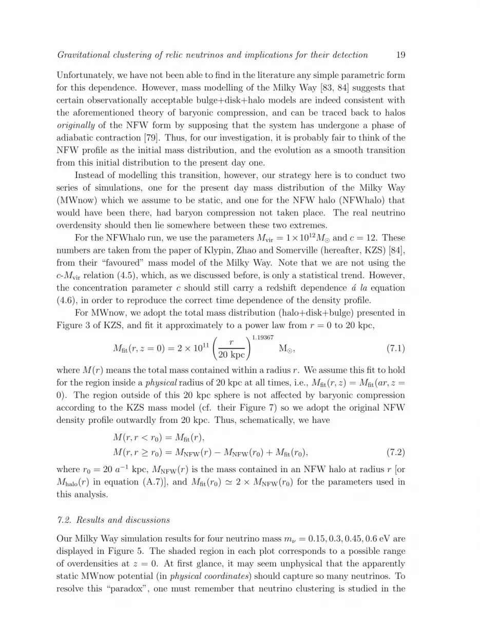
Figure 6. Momentum distribution of relic neutrinos at r⊕ for various neutrino masses.

The red (solid) line denotes the MWnow run, while the dashed line represents the

NFWhalo run. The relativistic Fermi–Dirac function is indicated by the dotted line.

The escape velocity vesc =√

2|φ(r⊕)| is 490 km s−1 and 450 km s−1 for MWnow

and NFWhalo respectively, corresponding to “escape momenta” yesc ≡ mνvesc/Tν,0 of

(5.9, 4.4, 3.0, 1.5) and (5.4, 4.1, 2.7, 1.4) for mν = (0.6, 0.45, 0.3, 0.15) eV.


bottom up, the mean momenta for the least clustered cases tend to be lower than the

Fermi–Dirac value 〈p〉 ≃ 3.15Tν,0, in contrast with the naıve expectation that clustering

is necessarily accompanied by an increase in the neutrinos’ average kinetic energy.

7.3. Tremaine–Gunn bound

It is interesting to compare our results with nominal bounds from phase space arguments.

By demanding the final coarse-grained distribution to be always less than the maximum

of the original fine-grained distribution, Tremaine and Gunn [86] argued in 1979 that if

neutrinos alone are to constitute the dark matter of a galactic halo, their mass must be

larger than 20 eV, assuming that the halo has a Maxwellian phase space distribution

as motivated by the theory of violent relaxation [85, 87, 88]. A modern version of

this bound, in which the assumption about the phase space distribution is relaxed and

which allows for contribution to the total gravitational potential from more than one

form of matter, can be found in reference [89]. The revised mass bound may be written,

alternatively, in the form of a constraint on the overdensity, which reads

nνnν

<m3νv

3esc

9ζ(3)T 3ν,0

. (7.3)

For the neutrino masses mν = (0.6, 0.45, 0.3, 0.15) eV, this expression evaluates to

(19, 8.0, 2.4, 0.3) and (15, 6.4, 1.8, 0.25) for MWnow and NFWhalo, respectively, at r⊕.

At first sight, some of our numerical results seem to have completely violated the

bound (7.3). But this cannot be, since we have seen explicitly that all of our final

coarse-grained distributions satisfy perfectly the constraint f ≤ max(f0). Furthermore,

an upper bound of 0.25 on the overdensity for a 0.15 eV neutrino is obviously nonsensical.

The answer, as the astute reader would have figured, lies in accounting. In the

derivation of (7.3), a semi-degenerate distribution has been summed only up to the

momentum state corresponding to the escape velocity of the system. Neutrinos with

higher momenta that could be hovering around in the vicinity have been completely

ignored. In contrast, in our calculations, it is of no concern to us whether or not the

relic neutrinos actually form bound states with the galaxy/halo. Therefore it is more

appropriate for us to sum every neutrino in sight, rather than imposing a cut-off at

vesc. However, if we had imposed such a cut-off, one can easily see from Figure 6 that

our overdensities would have just saturated the bound (7.3), so there is no conflict.

Nonetheless, this illustrates how nominal bounds such as (7.3) must be used with care.

Before we conclude this section, let us note that for an NFW halo, the bound (7.3)

can be written as

nνnν

<m3ν

9ζ(3)T 3ν,0

[2GMvir

g(c)

ln(1 + r/rs)

r

]3/2

≃ 0.58 ×(mν

eV

)3[(

Mvir

1012h−1M⊙

)(h−1Mpc

r

)ln(1 + r/rs)

g(c)

]3/2

, (7.4)

where the function g(c) is defined in equation (A.8) in the Appendix. Figure 7 shows

the bound as a function of radius for the various halo and neutrino masses considered


Figure 7. The Tremaine–Gunn bound on the neutrino overdensity for various halo

and neutrino masses (dashed lines). The red (solid) lines correspond to our N -1-body

results from section 5.

in section 5, along with the overdensities obtained from N -1-body simulations. We

find the limit (7.3) to be saturated for the lightest halo and neutrino masses (and also

some apparent violation of the bound due to different accounting). This explains why

some of the overdensities exhibit an almost m3ν dependence (cf. Figure 4). On the

other hand, the heaviest mν ,Mvir set is short of the bound by at least one order of

magnitude. This is also consistent with expectations: heavier halo and neutrino masses

give a higher escape momentum pesc, and higher momentum states are more difficult

to fill up to a semi-degenerate level, since there are less particles in these states in the


original Fermi–Dirac distribution to begin with.

8. Implications for detection

In this section, we determine the implications of our clustering results for the direct

detection of relic neutrinos, in contrast with the purely cosmological inferences discussed

in section 2. We consider various proposed detection methods based on scattering

processes, involving the relic neutrinos both as a beam and as a target. In particular,

we shall discuss (i) coherent elastic scattering of the relic neutrino flux off target

matter in a terrestrial detector (section 8.1), as well as (ii) the scattering of extremely

energetic particles (accelerator beams or cosmic rays) off the relic neutrinos as a target

(section 8.2).

8.1. Flux detection

The low average momentum 〈p〉 = 〈y〉 Tν,0 of the relic neutrinos (cf. Table 2)

corresponds to a (reduced) de Broglie wavelength of macroscopic dimension, λ– = 1/〈p〉 =

0.12 cm/〈y〉 (cf. Table 3). Therefore, one may envisage scattering processes in which

many target atoms act coherently [4, 5] over a macroscopic volume λ–3, so that the

reaction rate for elastic scattering becomes proportional to the square of the number of

target atoms in that volume. Compared to the case where the neutrinos are elastically

scattered coherently only on the individual nuclei of the target, the rate in this case is

enhanced by a huge factor of

NA

Aρt λ–

3 ≃ 6 × 1018(

100

A

)(ρt

g/cm3

)(λ–

0.1 cm

)3

, (8.1)

where NA is the Avogadro constant, A is the atomic mass, and ρt is the mass density

of the target material.+

By exploiting the above coherence effect, a practical detection scheme for the local

relic neutrino flux is based on the fact that a test body of density ρt at Earth will

experience a neutrino wind force through random neutrino scattering events, leading to

an acceleration [4, 5, 6, 93]

at ≃∑

ν,ν

nν vrel︸︷︷︸flux

4π

3N2A ρt r

3t σνN 2mν vrel︸︷︷︸

mom. transfer

≃ 2 × 10−28(nνnν

) (10−3 c

vrel

) (ρt

g/cm3

) (rt

h/(mνvrel)

)3

cm s−2, (8.2)

where σνN ≃ G2F m

2ν/π is the elastic neutrino–nucleon cross section, and vrel = 〈|v−v⊕|〉

is the mean velocity of the relic neutrinos in the rest system of the detector. Here,

v⊕ ≃ 2.3 × 102 km s−1 ≃ 7.7 × 10−4 c denotes the velocity of the Earth through the

+ In the case of coherent scattering, it is possible, in principle, to measure also the scattering amplitude

itself [90, 91, 92], which is linear in the Fermi coupling constant GF . However, one needs a large lepton

asymmetry for a non-negligible effect.


Table 3. Properties of the relic neutrinos at r⊕ for various neutrino masses from

the MWnow and NFWhalo runs (see text for definitions) relevant for their direct

detection. The first column shows the overdensities. Columns two, three and four show,

respectively, the mean absolute momenta, the associated mean reduced de Broglie

wavelengths and the mean absolute velocities (in units of c). The corresponding values

for a relativistic Fermi–Dirac distribution are displayed in row one.

nν

nν〈p〉 λ– = 1

〈p〉〈v〉

Relativistic Fermi–Dirac 1 5.3 × 10−4 eV 3.7 × 10−2 cm see (4.1)

NFWhalo, mν = 0.6 eV 12 7.2 × 10−4 eV 2.7 × 10−2 cm 1.2 × 10−3

NFWhalo, mν = 0.45 eV 6.4 5.9 × 10−4 eV 3.4 × 10−2 cm 1.3 × 10−3



MWnow, mν = 0.6 eV 20 8.5 × 10−4 eV 2.3 × 10−2 cm 1.4 × 10−3

MWnow, mν = 0.45 eV 10 6.7 × 10−4 eV 2.9 × 10−2 cm 1.5 × 10−3

MWnow, mν = 0.3 eV 4.4 5.4 × 10−4 eV 3.7 × 10−2 cm 1.8 × 10−3

MWnow, mν = 0.15 eV 1.6 4.9 × 10−4 eV 4.1 × 10−2 cm 3.2 × 10−3

Milky Way. Expression (8.2) is valid as long as the radius rt of the target is smaller than

the reduced de Broglie wavelength λ– = h/(mνvrel) of the relic neutrinos. Furthermore, it

applies only to Dirac neutrinos. For Majorana neutrinos, the acceleration is suppressed,

in comparison with (8.2), by a factor of (vrel/c)2 ≃ 10−6 for an unpolarised target, or

vrel/c ≃ 10−3 for a polarised one. A target size much larger than λ– can be exploited,

while avoiding destructive interference, by using foam-like [4] or laminated [5] materials.

Alternatively, grains of size ∼ λ– could be randomly embedded (with spacing ∼ λ–) in a

low density host material [94, 95].

To digest these estimates, we note that the smallest measurable acceleration at

present is >∼ 10−13 cm s−2, using conventional Cavendish-type torsion balances. Possible

improvements with currently available technology to a sensitivity of >∼ 10−23 cm s−2

have been proposed [96, 97]. However, such a sensitivity is still off the prediction (8.2)

by at least three orders of magnitude, as an inspection of the currently allowed range

of local relic neutrino overdensities in Table 3 reveals. Therefore, we conclude that

an observation of this effect will not be possible within the upcoming decade, but can

still be envisaged in the foreseeable future (thirty to forty years according to reference

[95], exploiting advances in nanotechnology), as long as our known light neutrinos are

Dirac particles. Should they turn out, in the meantime, to be Majorana particles, flux

detection via mechanical forces will be a real challenge.

Let us note finally that the background contribution to the acceleration (8.2)

from the solar pp neutrinos [flux ∼ 1011 cm−2s−1, 〈Eν〉 ∼ 0.3 MeV (e.g., [98])],

aν sunt ≃ 10−27 cm s−2 [6], may be rejected by directionality. The background from

weakly interacting massive particles (WIMPs χ, with mass mχ) [6],

aWIMPt ≃ nχ vrel︸︷︷︸

flux

NAA σχN 2mχ vrel︸︷︷︸mom. transfer

(8.3)


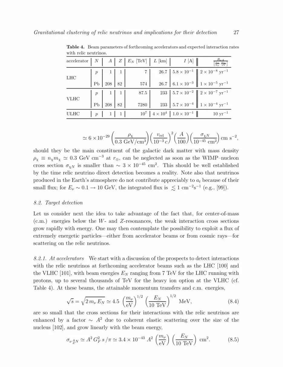
Table 4. Beam parameters of forthcoming accelerators and expected interaction rates

with relic neutrinos.

accelerator N A Z EN [TeV] L [km] I [A] RνA

[nνnν

mνeV ]

p 1 1 7 26.7 5.8 × 10−1 2 × 10−8 yr−1

LHC

Pb 208 82 574 26.7 6.1 × 10−3 1 × 10−5 yr−1

p 1 1 87.5 233 5.7 × 10−2 2 × 10−7 yr−1

VLHC

Pb 208 82 7280 233 5.7 × 10−4 1 × 10−4 yr−1

ULHC p 1 1 107 4 × 104 1.0 × 10−1 10 yr−1

≃ 6 ×10−29

(ρχ

0.3 GeV/cm3

)(vrel

10−3 c

)2( A

100

)(σχN

10−45 cm2

)cm s−2,

should they be the main constituent of the galactic dark matter with mass density

ρχ ≡ nχmχ ≃ 0.3 GeV cm−3 at r⊕, can be neglected as soon as the WIMP–nucleon

cross section σχN is smaller than ∼ 3 × 10−45 cm2. This should be well established

by the time relic neutrino direct detection becomes a reality. Note also that neutrinos

produced in the Earth’s atmosphere do not contribute appreciably to at because of their

small flux; for Eν ∼ 0.1 → 10 GeV, the integrated flux is <∼ 1 cm−2s−1 (e.g., [99]).

8.2. Target detection

Let us consider next the idea to take advantage of the fact that, for center-of-mass

(c.m.) energies below the W - and Z-resonances, the weak interaction cross sections

grow rapidly with energy. One may then contemplate the possibility to exploit a flux of

extremely energetic particles—either from accelerator beams or from cosmic rays—for

scattering on the relic neutrinos.

8.2.1. At accelerators We start with a discussion of the prospects to detect interactions

with the relic neutrinos at forthcoming accelerator beams such as the LHC [100] and

the VLHC [101], with beam energies EN ranging from 7 TeV for the LHC running with

protons, up to several thousands of TeV for the heavy ion option at the VLHC (cf.

Table 4). At these beams, the attainable momentum transfers and c.m. energies,

√s =

√2mν EN ≃ 4.5

(mν

eV

)1/2 ( EN10 TeV

)1/2

MeV, (8.4)

are so small that the cross sections for their interactions with the relic neutrinos are

enhanced by a factor ∼ A2 due to coherent elastic scattering over the size of the

nucleus [102], and grow linearly with the beam energy,

σν AZN ≃ A2G2

F s /π ≃ 3.4 × 10−43 A2(mν

eV

) (EN

10 TeV

)cm2. (8.5)


This leads to a scattering rate [103, 104, 105]

Rν AZN ≃

∑

ν,ν

nν σν AZN L I/(Z e) (8.6)

≃ 2 × 10−8(nνnν

)(mν

eV

)A2

Z

(EN

10 TeV

) (L

100 km

) (I

0.1 A

)yr−1,

for a beam of particles AZN , with charge Z e, length L and current I. In view of the

currently allowed range of local relic neutrino overdensities displayed in Table 3, and

the beam parameters of the next generation of accelerators summarised in Table 4,

the expected rate (8.6) is clearly too small to give rise to an observable effect in

the foreseeable future. The extremely energetic 574 TeV lead beam at the LHC will

have less than 10−4 interactions per year with relic neutrinos, for mν <∼ 0.6 eV and,

correspondingly, nν/nν <∼ 20. Even a lead acceleration option for the VLHC, with

EN ≃ 7280 TeV (or, equivalently, 35 TeV per nucleon) and a current I ≃ 5.7×10−4 A (a

hundredth of the nominal current of the p running mode) will give less than 10−3 events

per year for the most optimistic neutrino mass scenario. Thus, there is little hope, in

the foreseeable future, to detect relic neutrino using terrestrial accelerator beams.

Let us nevertheless dream about the far future, in which an Ultimate Large Hadron

Collider (ULHC) exists and is able to accelerate protons to energies above 107 TeV∗in a ring of ultimate circumference L ≃ 4 × 104 km around the Earth, thus leading

to an interaction rate of more than one event per year (cf. Table 4). Even under

these most optimistic circumstances, is it possible to reliably detect these interactions?

Clearly, elastic scattering of the beam particles with the relic neutrinos—one of the

contributions to the rate (8.6)—will be next to impossible to detect because of the

small momentum transfers involved (∼ 1 GeV at EN ∼ 107 TeV). A very promising

alternative is to consider again a heavy ion beam, and to exploit the contribution of the

inverse beta decay reaction,

AZN + νe → A

Z+1N + e− , (8.7)

to the rate (8.6). This reaction changes the charge of the nucleus, causing it to follow an

extraordinary trajectory and finally to exit the machine such that it becomes susceptible

to detection [104, 109]. A detection of this reaction would also clearly demonstrate that

a neutrino was involved in the scattering.

8.2.2. With cosmic rays In the meantime, until the ULHC has been constructed, target

detection of the relic neutrinos has to rely on extremely energetic cosmic rays. In

fact, cosmic rays with up energies up to Ecr ∼ 1020 eV have been seen by air shower

∗ Note that a collider at this energy has to be built anyhow if one wishes to explore the “intermediate”

scale (MEW MGUT)1/2 ∼ 1010 GeV between the electroweak scale MEW ∼ 1 TeV and the scale of grand

unification MGUT ∼ 1017 GeV. The intermediate scale is exploited in many schemes of supersymmetry

breaking (e.g., [106]) and in seesaw mechanisms for neutrino masses [107, 108].


observatories. The corresponding c.m. energies are

√s =

√2mν Ecr ≃ 14

(mν

eV

)1/2 ( Ecr

1020 eV

)1/2

GeV (8.8)

when scattering off the relic neutrinos. These energies are not too far from the W - and

Z-resonances, at which the electroweak cross sections become sizeable. Indeed, it was

pointed out long ago by Weiler [7, 8] (for earlier suggestions, see [110, 111, 112, 113, 114])

that the resonant annihilation of extremely energetic cosmic neutrinos (EECν) with relic

anti-neutrinos (and vice versa) into Z-bosons appears to be a unique process having

sensitivity to the relic neutrinos. On resonance,

Eresν =

m2Z

2mν≃ 4 × 1021

(eV

mν

)eV, (8.9)

the associated cross section is enhanced by several orders of magnitude,

〈σann〉 =∫ds/m2

Z σZνν(s) ≃ 2π

√2GF ≃ 4 × 10−32 cm2, (8.10)

leading to a “short” mean free path ℓν = (nν 〈σann〉)−1 ≃ 1.4 × 105 Mpc which is

only about 48 h times the Hubble distance. Neglecting cosmic evolution effects, this

corresponds to an annihilation probability for EECν from cosmological distances on the

relic neutrinos of 2 h−1%.

The signatures of annihilation are (i) absorption dips [7, 8, 9] (see also [115, 116,

117]) in the EECν spectrum at the resonant energies, and (ii) emission features [10,

11, 12, 13, 14] (Z-bursts) as protons (or photons) with energies spanning a decade

or more above the predicted Greisen–Zatsepin–Kuzmin (GZK) cutoff at EGZK ≃4 × 1019 eV [118, 119]. This is the energy beyond which the CMB is absorbing to

nucleons due to resonant photopion production.♯

The possibility to confirm the existence of relic neutrinos within the next

decade from a measurement of the aforementioned absorption dips in the EECν

flux was recently investigated in [9]. Presently planned neutrino detectors (Pierre

Auger Observatory [124], IceCube [125], ANITA [126], EUSO [127], OWL [128], and

SalSA [129]) operating in the energy regime above 1021 eV appear to be sensitive

enough to lead us, within the next decade, into an era of relic neutrino absorption

spectroscopy, provided that the flux of the EECν at the resonant energies is close to

current observational bounds and the neutrino mass is sufficiently large, mν >∼ 0.1 eV.

In this case, the associated Z-bursts must also be seen as post-GZK events at the

planned cosmic ray detectors (Pierre Auger Observatory, EUSO, and OWL).

What are the implications of relic neutrino clustering for absorption and emission

spectroscopy? Firstly, absorption spectroscopy is predominantly sensitive to the relic

neutrino background at early times, with the depths of the absorption dips determined

largely by the higher number densities at large redshifts (z ≫ 1). Since neutrinos do

not cluster significantly until after z <∼ 2, clustering at recent times can only show up as

♯ The association of Z-bursts with the mysterious cosmic rays observed above EGZK is a controversial

possibility [10, 11, 12, 13, 14, 120, 121, 122, 123].


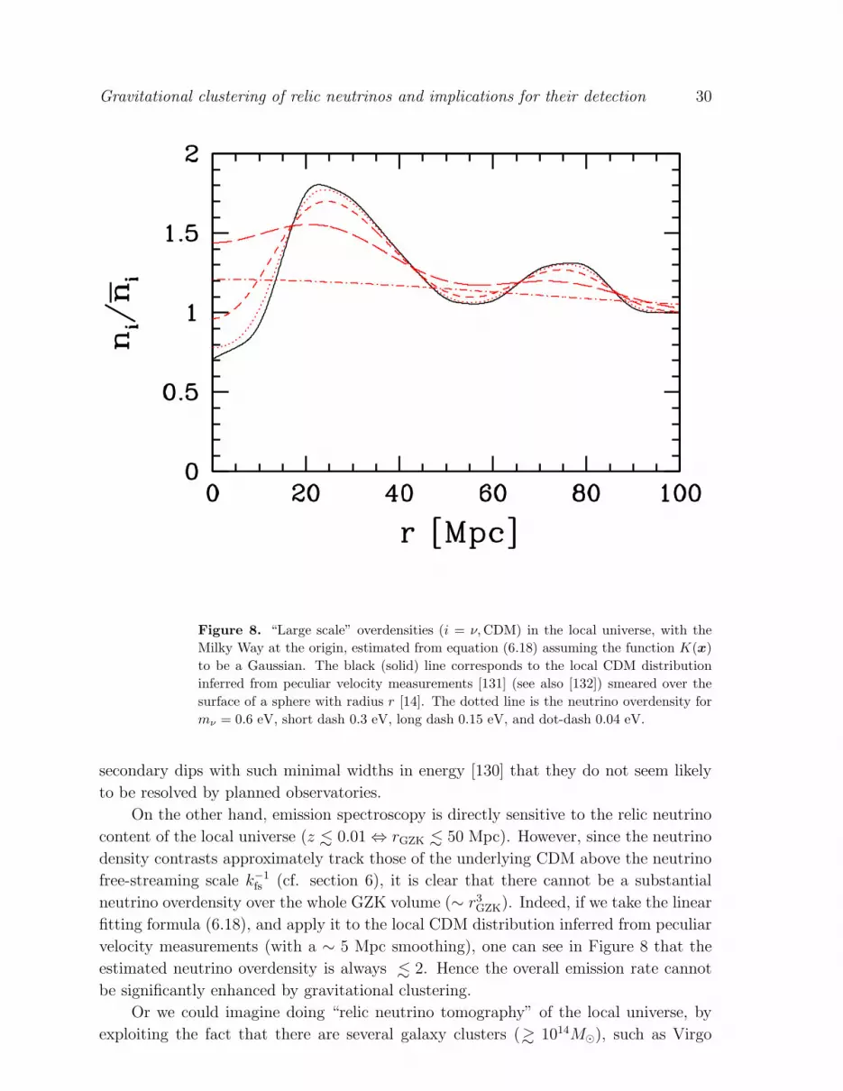
Figure 8. “Large scale” overdensities (i = ν, CDM) in the local universe, with the

Milky Way at the origin, estimated from equation (6.18) assuming the function K(x)

to be a Gaussian. The black (solid) line corresponds to the local CDM distribution

inferred from peculiar velocity measurements [131] (see also [132]) smeared over the

surface of a sphere with radius r [14]. The dotted line is the neutrino overdensity for

mν = 0.6 eV, short dash 0.3 eV, long dash 0.15 eV, and dot-dash 0.04 eV.

secondary dips with such minimal widths in energy [130] that they do not seem likely

to be resolved by planned observatories.

On the other hand, emission spectroscopy is directly sensitive to the relic neutrino

content of the local universe (z <∼ 0.01 ⇔ rGZK <∼ 50 Mpc). However, since the neutrino

density contrasts approximately track those of the underlying CDM above the neutrino

free-streaming scale k−1fs (cf. section 6), it is clear that there cannot be a substantial

neutrino overdensity over the whole GZK volume (∼ r3GZK). Indeed, if we take the linear

fitting formula (6.18), and apply it to the local CDM distribution inferred from peculiar

velocity measurements (with a ∼ 5 Mpc smoothing), one can see in Figure 8 that the

estimated neutrino overdensity is always <∼ 2. Hence the overall emission rate cannot

be significantly enhanced by gravitational clustering.

Or we could imagine doing “relic neutrino tomography” of the local universe, by

exploiting the fact that there are several galaxy clusters (>∼ 1014M⊙), such as Virgo


(distance ∼ 15 Mpc) and Centaurus (∼ 45 Mpc), within the GZK zone with significant

neutrino clustering (cf. Figure 1). One could conceivably search for directional

dependences in the emission events as a signature of EECν annihilating on relic anti-

neutrinos (and vice versa). For example, AGASA has an angular resolution of ∼ 2

[133]. This is already sufficient to resolve the internal structures of, say, the Virgo cluster

(distance ∼ 15 Mpc, Mvir ∼ 8×1014M⊙) which spans some 10 across the sky. Using our

N -1-body clustering results in Figure 1, the average neutrino overdensity along the line

of sight towards and up to Virgo is estimated to be ∼ 45 and ∼ 5 for mν = 0.6 eV and

0.15 eV respectively, given an angular resolution of ∼ 2. The corresponding increases

in the number of events coming from the direction of the Virgo cluster relative to the

unclustered case, assuming an isotropic distribution of EECν sources, are given roughly

by the same numbers, since protons originating from ∼ 15 Mpc away arrive at Earth

approximately unattenuated. The numbers improve to ∼ 55 and ∼ 8 respectively with

a finer ∼ 1 angular resolution.

Note that our estimates here are generally a factor of few higher than the predictions

of SM. This is expected, because the linear method adopted in their analysis cannot

account for additional clustering from nonlinear effects, as we demonstrated in section 6.

9. Conclusion

We have conducted a systematic and exhaustive study of the gravitational clustering

of big bang relic neutrinos onto existing CDM and baryonic structures within the flat

ΛCDM model, with the aim of understanding their clustering properties on galactic

and sub-galactic scales for the purpose of designing possible scattering-based detection

methods. Our main computational tools are (i) a restricted, N -1-body method

(section 5), in which we neglect the gravitational interaction between the neutrinos

and treat them as test particles moving in an external potential generated by the

CDM/baryonic structures, and (ii) a semi-analytical, linear technique (section 6), which

requires additional assumptions about the neutrino phase space distribution. In both

cases, the CDM/baryonic gravitational potentials are calculated from parametric halo

density profiles from high resolution N -body studies [60, 61] (section 4) and/or from

realistic mass distributions reconstructed from observational data (e.g., [84, 131]).

Using these two computational techniques, we track the relic neutrinos’ accretion

onto CDM halos ranging from the galaxy to the galaxy cluster variety (Mvir ∼ 1012 →1015M⊙), and determine the neutrino number densities on scales ∼ 1 → 1000 kpc for

neutrino masses satisfying current constraints (2.1) from CMB and LSS (Figures 1 and

2). Because we can simulate only a finite set of halo and neutrino parameters, we

provide also additional plots illustrating the approximate dependences of the neutrino

overdensities on the halo and neutrino masses (Figures 3 and 4). These can be used for

interpolation between simulation results. Furthermore, we find that the linear technique

systematically underestimates the neutrino overdensities over the whole range of halo

and neutrino masses considered in this study (Figure 1). Reconciliation with N -1-body


simulations can only be achieved if we impose a smoothing scale of >∼ 1 Mpc, or if the

overdensity is no more than three or four. We therefore conclude that the linear theory

does not generally constitute a faithful approximation to the Vlasov equation in the

study of neutrino clustering on galactic and sub-galactic scales (<∼ 50 kpc). However,

it may still be useful for finding the minimum effects of neutrino clustering in other

contexts not considered in this work (e.g., the nonlinear matter power spectrum [134]).

Next we apply our N -1-body method to calculate the relic neutrino number

density in the Milky Way (section 7), especially their phase space distribution in our

local neighbourhood at Earth r⊕, taking also into account contributions to the total

gravitational potential from the galactic bulge and disk. We find a maximum overdensity

of ∼ 20 per neutrino flavour in our immediate vicinity, provided that the neutrino mass is

at its current upper limit of 0.6 eV (Table 2 and Figure 5). For neutrino masses less than

0.15 eV, the expected overdensity from gravitational clustering is less than two. The

associated coarse-grained momentum spectra show varying degrees of deviation from

the relativistic Fermi–Dirac function, but share a common feature that they are semi-

degenerate, with phase space density f ∼ 1/2, up to the momentum state corresponding

to the escape velocity from the Milky Way at r⊕ (Figure 6). This means that the neutrino

number densities we have calculated here for r⊕ are already the highest possible, given

the neutrino mass, without violating phase space constraints (e.g., [85, 89]). In order to

attain even higher densities, one must now appeal to non-standard theories (e.g., [135]).

In terms of scattering-based detection possibilities, this meager enhancement in

the neutrino number density in the Milky Way from gravitational clustering means

that relic neutrinos are still far from being detected in fully earthbound laboratory

experiments. For flux detection methods based on coherent elastic scattering of relic

neutrinos off target matter in a terrestrial detector (section 8.1), a positive detection

could be thirty to forty years away [95], provided that light neutrinos are Dirac particles.

For light Majorana neutrinos, another ∼ 103 times more sensitivity would be required

in the detector for a positive signal. Target detection methods using accelerator beams

(section 8.2.1) seem equally hopeless, unless the accelerator is the size of the Earth and

operates at an energy of ∼ 107 TeV (Table 4).

Meanwhile, target detection using extremely energetic cosmic neutrinos (EECν,>∼ 1021 eV) remains the only viable means to confirm the existence of big bang relic

neutrinos within the next decade or so (section 8.2.2). Resonant annihilation of EECν

on relic neutrinos can be revealed as absorption dips in the EECν flux (e.g., [9]), or as

emission features in the Z-decay products. However, since absorption spectroscopy is

largely insensitive to late time (z <∼ 2) relic neutrino clustering, our findings here have

little impact on the conclusions of [9]. On the other hand, emission spectroscopy is

sensitive to the relic neutrino content of the local GZK zone, VGZK ∼ 503 Mpc3. While

we find no significant large scale clustering within VGZK (Figure 8) and therefore no

significant enhancement in the overall emission rates, it is still conceivable to exploit the

considerable neutrino overdensities in nearby galaxy clusters, and search for directional

dependences in the post-GZK emission events. For the Virgo cluster, for example,


we estimate the event rate from the central 1 region to be ∼ 55 and ∼ 8 times the

unclustered rate for neutrino mass mν = 0.6 eV and 0.15 eV respectively, assuming

an isotropic distribution of EECν sources. [Our estimates differ by a factor of a few

from the predictions of [25] because their linear technique fails to account for additional

clustering from nonlinear effects, as we have demonstrated in this study (section 6)].

Planned observatories such as the Pierre Auger Observatory [124], EUSO [127] and

OWL [128] will have sufficient angular resolution to, in principle, see this enhancement.

However, considering the rapidly improving constraints on both the EECν flux and

neutrino masses, it remains to be seen if the enhancement can indeed be observed with

enough statistical significance.

Acknowledgments

We would like to thank David Cerdeno, Pasquale Di Bari, Birgit Eberle, Jan Hamann,

Oleg Lebedev, Helmut Mais, and Thomas Reiter for useful discussions.

Appendix A. Details of N-1-body simulations

We give in this appendix a detailed discussion of the techniques used in our N -1-body

simulations.

Appendix A.1. Hamilton’s equations

Following [59], we begin with a Lagrangian L(x, x, τ) = a[

12mνv

2 −mνφ(|x|, τ)]

for a

test particle (neutrino) with massmν and peculiar velocity v ≡ x moving in a spherically

symmetric gravitational potential well φ(x, τ) generated by the CDM halo. Because of

spherical symmetry, the motion of the test particle is confined to a plane. This allows

us to switch to polar coordinates r, θ to obtain

L(r, θ, r, θ, τ) = a[1

2mν(r

2 + r2θ2) −mνφ(r, τ)], (A.1)

and eliminate two superfluous variables in the process. The canonical momenta

conjugate to r and θ are pr ≡ ∂L/∂r = amν r and ℓ ≡ rpθ ≡ ∂L/∂θ = amνr2θ

respectively, leading to the Hamiltonian

H(r, θ, pr, ℓ, τ) =1

2amν

[p2r +

ℓ2

r2

]+ amνφ(r, τ), (A.2)

and hence Hamilton’s equations

dr

dτ=

pramν

,dθ

dτ=

ℓ

amνr2,

dprdτ

=ℓ2

amνr3− amν

∂φ

∂r,

dℓ

dτ= 0, (A.3)

where the last equality expresses the conservation of conjugate comoving angular

momentum ℓ.


For computational purposes, it is convenient to rewrite the set of differential

equations (A.3) in terms of redshift z and the normalised quantities ur ≡ pr/mν = ar

and uθ ≡ ℓ/mν = ar2θ, thus rendering (A.3) into the form

dr

dz= −ur

a,

dθ

dz= − uθ

ar2,

durdz

= −1

a

(u2θ

r3− a2∂φ

∂r

),

duθdz

= 0, (A.4)

where a = (1 + z)−1 and a = H0

√a−1 Ωm,0 + a2 ΩΛ,0 are, respectively, the scale factor

and the expansion rate, the latter of which is determined by the present day Hubble

constant H0 and the cosmological model in hand.

The gravitational potential φ(r, τ) obeys the Poisson equation

∇2φ→ 1

r2

∂

∂r

(r2∂φ

∂r

)= 4πGa2ρm(τ)δm(r, τ). (A.5)

Since we are treating the CDM halo as a density perturbation sitting on top of a uniform

background, i.e., ρm(τ)δm(r, τ) → ρhalo(r), we have the following (partial) solution:

∂φ

∂r=

4πGa2

r2

∫ r

0ρhalo(r

′, τ)r′2dr′ =G

ar2Mhalo(r), (A.6)

where Mhalo(r) is the physical mass contained in a sphere of radius r. For an NFW halo,

Mhalo(r) = 4πa3ρsr3sg(x) = Mvirg(x)/g(c), x = r/rs, (A.7)

g(x) = ln(1 + x) − x

1 + x, (A.8)

c =9

1 + z

(Mvir

1.5 × 1013h−1M⊙

)−0.13

, (A.9)

rs =1

c

(3

4π

Mvir

ρm,0∆vir

)1/3

= 9.51 × 10−1 c−1Ω−1/3m,0 ∆

−1/3vir

(Mvir

1012h−1M⊙

)1/3

h−1Mpc. (A.10)

The meanings of these various symbols are explained in section 4.

Appendix A.2. Discretising the initial phase space distribution

The number of neutrinos at some initial time τi in the interval (x,p) → (x+dx,p+dp)

is defined to be

dN = f(x,p, τi)d3x d3p. (A.11)

We assume the initial phase space distribution to be isotropic and homogeneous, i.e.,

f(x,p, τi) = f0(p). This initial homogeneity implies that the ensemble’s subsequent

evolution under a spherically symmetric potential will depend only on the initial radial

distance r, radial momentum pr, and transverse momentum pT =√p2 − p2

r. Thus we

may rewrite the phase space volume element as

d3x→ r2 sin θ dθ dφ dr, d3p→ pT dpT dpr dϕ, (A.12)


with r ∈ [0,∞), θ ∈ [0, π], φ ∈ [0, 2π), and pT ∈ [0,∞), pr ∈ (−∞,∞), ϕ ∈ [0, 2π).

In an ideal and perfectly deterministic calculation, one would track the motion

of every particle for every occupied combination of r, pr and pT . This is obviously

impossible in practice; one must therefore resort to simulating only a representative set

of particles and endow each with a “weight” according to the phase space region from

which the particle is drawn. We show below how this weight is calculated.††Suppose that a point particle initially at (r, pr, pT ) is representative for all particles

in the initial phase space interval (ra, pr,a, pT,a) → (rb, pr,b, pT,b). The weight carried by

this representative particle is defined as

wi ≡∫ rb,pr,b,pT,b

ra,pr,a,pT,a

∫

θ,φ,ϕdN, (A.13)

where∫θ,φ,ϕ means summing over all θ, φ and ϕ, which is simple:

∫θ,φ,ϕ sin θ dθ dφ dϕ =

8π2. The spatial integral over r is also readily calculable. The remaining phase space

integral∫ pr,b,pT,b

pr,a,pT,af(p)pTdpTdpr can be solved by way of the parameterisation pr = p cosψ,

and pT = p sinψ, and hence

pT dpTdpr → p2 sinψ dψ, p ∈ [0,∞), ψ ∈ [0, π). (A.14)

Thus the weight carried by a point particle centred on and representing the interval

(ra, pa, ψa) → (rb, pb, ψb) is given by

wi = 8π2T 3ν,0

∫ rb

rar2dr

∫ yb

ya

f(y)y2dy∫ ψb

ψa

sinψdψ, (A.15)

where y = p/Tν,0 is a dimensionless momentum variable.

Appendix A.3. Kernel method for density profile estimation

We construct the neutrino density profiles from the discrete outputs of our N -1-body

simulations using the kernel method of [65] and [70], which we reproduce here for

completeness.

The number density corresponding to a set of particles is estimated to be

n(r) =N∑

i=1

wih3K[1

h|r − ri|

], (A.16)

where wi is the weight carried by the ith particle, h is the window width, and K is a

normalised kernel such as the Gaussian kernel,

K(y) =1

(2π)3/2e−y

2/2. (A.17)

In order to obtain a spherically symmetric profile, we smear every particle around the

surface of a sphere with radius ri centred on r = 0. The spherically symmetric density

estimate is then

n(r) =N∑

i=1

wih3K(r, ri, h), (A.18)

††We note for completeness that the concept of super particles with equal masses or, in our language,

weights is adopted in most full scale N -body simulations [15]. The representative point particles are

drawn randomly from the initial phase space distribution.


with

K(r, ri, h) ≡1

4π

∫dφ∫dθ sin θK

(h−1

√r2 + r2

i − 2rri cos θ). (A.19)

Substituting for the Gaussian kernel, we get

K(r, ri, h) =1

2(2π)3/2

h2

rri

[e−(r−ri)

2/2h2 − e−(r+ri)2/2h2

]. (A.20)

The optimal choice of h generally depends on the underlying function n(r) [70]. In our

analysis, however, a constant h is adopted for simplicity. Our momentum distributions

in section 7 are also constructed with this kernel method.

References

[1] S. Eidelman et al. [Particle Data Group Collaboration], Phys. Lett. B 592 (2004) 1.

[2] S. Hannestad, New J. Phys. 6 (2004) 108 [arXiv:hep-ph/0404239].

[3] G. L. Fogli, E. Lisi, A. Marrone, D. Montanino, A. Palazzo and A. M. Rotunno, eConf C030626

(2003) THAT05 [arXiv:hep-ph/0310012].

[4] B. F. Shvartsman, V. B. Braginsky, S. S. Gershtein, Y. B. Zeldovich and M. Y. Khlopov, JETP

Lett. 36 (1982) 277 [Pisma Zh. Eksp. Teor. Fiz. 36 (1982) 224].

[5] P. F. Smith and J. D. Lewin, Phys. Lett. B 127 (1983) 185.

[6] G. Duda, G. Gelmini and S. Nussinov, Phys. Rev. D 64 (2001) 122001 [arXiv:hep-ph/0107027].

[7] T. J. Weiler, Phys. Rev. Lett. 49 (1982) 234.

[8] T. J. Weiler, Astrophys. J. 285 (1984) 495.

[9] B. Eberle, A. Ringwald, L. Song and T. J. Weiler, Phys. Rev. D 70 (2004) 023007

[arXiv:hep-ph/0401203].

[10] D. Fargion, B. Mele and A. Salis, Astrophys. J. 517 (1999) 725 [arXiv:astro-ph/9710029].

[11] T. J. Weiler, Astropart. Phys. 11 (1999) 303 [arXiv:hep-ph/9710431].

[12] S. Yoshida, G. Sigl and S. J. Lee, Phys. Rev. Lett. 81 (1998) 5505 [arXiv:hep-ph/9808324].

[13] Z. Fodor, S. D. Katz and A. Ringwald, Phys. Rev. Lett. 88 (2002) 171101 [arXiv:hep-ph/0105064].

[14] Z. Fodor, S. D. Katz and A. Ringwald, JHEP 0206 (2002) 046 [arXiv:hep-ph/0203198].

[15] R. W. Hockney and J. W. Eastwood, Computer Simulation Using Particles (McGraw–Hill, New

York, 1981).

[16] G. Efstathiou, M. Davis, C. S. Frenk and S. D. M. White, Astrophys. J. Suppl. 57 (1985) 241.

[17] E. Bertschinger, Ann. Rev. Astron. Astrophys. 36 (1998) 599.

[18] A. Klypin, in Modern Cosmology, edited by S. Bonometto, V. Gorini, and U. Moschella (IOP,

Bristol, 2002), p. 420.

[19] C. P. Ma and E. Bertschinger, Astrophys. J. 434 (1994) L5 [arXiv:astro-ph/9407085].

[20] Y. P. Jing and L. Z. Fang, Astrophys. J. 432 (1994) 438 [arXiv:astro-ph/9403012].

[21] R. A. C. Croft and G. Efstathiou, Mon. Not. Roy. Astron. Soc. 268 (1994) L23.

[22] C. Walter and A. Klypin, Astrophys. J. 462 (1996) 13 [arXiv:astro-ph/9507074].

[23] L. Kofman, A. Klypin, D. Pogosian and J. P. Henry, Astrophys. J. 470 (1996) 102

[arXiv:astro-ph/9509145].

[24] A. Blanchard, M. Douspis, M. Rowan-Robinson and S. Sarkar, Astron. Astrophys. 412 (2003) 35


[25] S. Singh and C. P. Ma, Phys. Rev. D 67 (2003) 023506 [arXiv:astro-ph/0208419].

[26] J. A. Sellwood, Ann. Rev. Astron. Astrophys. 25 (1987) 151.

[27] G. Abbiendi et al. [OPAL Collaboration], Eur. Phys. J. C 19 (2001) 587 [arXiv:hep-ex/0012018].

[28] C. Weinheimer, Nucl. Phys. Proc. Suppl. 118 (2003) 279.

[29] V. M. Lobashev et al., Nucl. Phys. Proc. Suppl. 91 (2001) 280.

[30] A. Osipowicz et al. [KATRIN Collaboration], arXiv:hep-ex/0109033.

http://arXiv.org/abs/hep-ph/0404239




http://arXiv.org/abs/astro-ph/9710029











http://arXiv.org/abs/hep-ex/0012018



[31] M. Tegmark et al. [SDSS Collaboration], Phys. Rev. D 69 (2004) 103501 [arXiv:astro-ph/0310723].

[32] G. L. Fogli, E. Lisi, A. Marrone, A. Melchiorri, A. Palazzo, P. Serra and J. Silk,

arXiv:hep-ph/0408045.

[33] S. Hannestad, JCAP 0305 (2003) 004 [arXiv:astro-ph/0303076].

[34] C. L. Bennett et al., Astrophys. J. Suppl. 148 (2003) 1 [arXiv:astro-ph/0302207].

[35] M. Tegmark et al. [SDSS Collaboration], Astrophys. J. 606 (2004) 702 [arXiv:astro-ph/0310725].

[36] J. A. Peacock et al., Nature 410 (2001) 169 [arXiv:astro-ph/0103143].

[37] W. L. Freedman et al., Astrophys. J. 553 (2001) 47 [arXiv:astro-ph/0012376].

[38] R. A. Knop et al., Astrophys. J. 598 (2003) 102 [arXiv:astro-ph/0309368].

[39] U. Seljak et al., arXiv:astro-ph/0406594.

[40] U. Seljak et al., arXiv:astro-ph/0407372.

[41] D. N. Spergel et al., Astrophys. J. Suppl. 148 (2003) 175 [arXiv:astro-ph/0302209].

[42] Ø. Elgarøy and O. Lahav, JCAP 0304 (2003) 004 [arXiv:astro-ph/0303089].

[43] P. Crotty, J. Lesgourgues and S. Pastor, Phys. Rev. D 69 (2004) 123007 [arXiv:hep-ph/0402049].

[44] V. Barger, D. Marfatia and A. Tregre, Phys. Lett. B 595 (2004) 55 [arXiv:hep-ph/0312065].

[45] K. N. Abazajian and S. Dodelson, Phys. Rev. Lett. 91 (2003) 041301 [arXiv:astro-ph/0212216].

[46] M. Kaplinghat, L. Knox and Y. S. Song, Phys. Rev. Lett. 91 (2003) 241301


[47] S. Hannestad and G. Raffelt, JCAP 0404 (2004) 008 [arXiv:hep-ph/0312154].

[48] P. Crotty, J. Lesgourgues and S. Pastor, Phys. Rev. D 67 (2003) 123005 [arXiv:astro-ph/0302337].

[49] E. Pierpaoli, Mon. Not. Roy. Astron. Soc. 342 (2003) L63 [arXiv:astro-ph/0302465].

[50] V. Barger, J. P. Kneller, H. S. Lee, D. Marfatia and G. Steigman, Phys. Lett. B 566 (2003) 8


[51] R. Bowen, S. H. Hansen, A. Melchiorri, J. Silk and R. Trotta, Mon. Not. Roy. Astron. Soc. 334

(2002) 760 [arXiv:astro-ph/0110636].

[52] S. Bashinsky and U. Seljak, Phys. Rev. D 69 (2004) 083002 [arXiv:astro-ph/0310198].

[53] R. H. Cyburt, B. D. Fields, K. A. Olive and E. Skillman, arXiv:astro-ph/0408033.

[54] A. Cuoco, F. Iocco, G. Mangano, G. Miele, O. Pisanti and P. D. Serpico, arXiv:astro-ph/0307213.

[55] V. Barger, J. P. Kneller, P. Langacker, D. Marfatia and G. Steigman, Phys. Lett. B 569 (2003)

123 [arXiv:hep-ph/0306061].

[56] A. D. Dolgov, S. H. Hansen, S. Pastor, S. T. Petcov, G. G. Raffelt and D. V. Semikoz, Nucl. Phys.

B 632 (2002) 363 [arXiv:hep-ph/0201287].

[57] Y. Y. Y. Wong, Phys. Rev. D 66 (2002) 025015 [arXiv:hep-ph/0203180].

[58] K. N. Abazajian, J. F. Beacom and N. F. Bell, Phys. Rev. D 66 (2002) 013008


[59] E. Bertschinger, in Les Houches Cosmology 1993, pp. 273-348, arXiv:astro-ph/9503125.

[60] J. F. Navarro, C. S. Frenk and S. D. M. White, Astrophys. J. 462 (1996) 563


[61] J. F. Navarro, C. S. Frenk and S. D. M. White, Astrophys. J. 490 (1997) 493.

[62] A. V. Kravtsov, A. A. Klypin and A. M. Khokhlov, Astrophys. J. Suppl. 111 (1997) 73


[63] Y. P. Jing, Astrophys. J. 535 (2000) 30 [arXiv:astro-ph/9901340].

[64] J. S. Bullock et al., Mon. Not. Roy. Astron. Soc. 321 (2001) 559 [arXiv:astro-ph/9908159].

[65] D. Reed et al., Mon. Not. Roy. Astron. Soc. 346 (2003) 565 [arXiv:astro-ph/0312544].

[66] B. Moore, T. Quinn, F. Governato, J. Stadel and G. Lake, Mon. Not. Roy. Astron. Soc. 310 (1999)

1147 [arXiv:astro-ph/9903164].

[67] Y. P. Jing and Y. Suto, Astrophys. J. Lett. 529 (2000) L69 [arXiv:astro-ph/9909478].

[68] C. P. Ma and J. N. Fry, Astrophys. J. 543 (2000) 503 [arXiv:astro-ph/0003343].

[69] G. L. Bryan and M. L. Norman, Astrophys. J. 495 (1998) 80 [arXiv:astro-ph/9710107].

[70] D. Merritt and B. Tremblay, Astron. J. 108 (1994) 514.

[71] I. H. Gilbert, Astrophys. J. 144 (1966) 233.








































[72] J. R. Bond and A. S. Szalay, Astrophys. J. 274 (1983) 443.

[73] R. H. Brandenberger, N. Kaiser and N. Turok, Phys. Rev. D 36 (1987) 2242.

[74] E. Bertschinger and P. N. Watts, Astrophys. J. 328 (1988) 23.

[75] L. Perivolaropoulos, R. H. Brandenberger and A. Stebbins, Phys. Rev. D 41 (1990) 1764.

[76] S. Setayeshgar, SB thesis (MIT, 1990).

[77] J. Binney and S. Tremaine, Galactic Dynamics (Princeton University Press, Princeton NJ, 1987)

[78] S. D. M. White and M. J. Rees, Mon. Not. Roy. Astro. Soc. 183 (1978) 341.

[79] G. R. Blumenthal, S. M. Faber, R. Flores and J. R. Primack, Astrophys. J. 301 (1986) 27.

[80] R. Flores, J. R. Primack, G. R. Blumenthal and S. M. Faber, Astrophys. J. 412 (1993) 443.

[81] H. J. Mo, S. Mao and S. D. M. White, Mon. Not. Roy. Astron. Soc. 295 (1998) 319


[82] O. Y. Gnedin, A. V. Kravtsov, A. A. Klypin and D. Nagai, arXiv:astro-ph/0406247.

[83] W. Dehnen and J. Binney, Mon. Not. Roy. Astro. Soc. 294 (1998) 429 [arXiv:astro-ph/9612059].

[84] A. Klypin, H. Zhao and R. S. Somerville, Astrophys. J. 573 (2002) 597 [arXiv:astro-ph/0110390].

[85] D. Lynden-Bell, Mon. Not. Roy. Astron. Soc. 136 (1967) 101.

[86] S. Tremaine and J. E. Gunn, Phys. Rev. Lett. 42 (1979) 407.

[87] F. H. Shu, Astrophys. J. 225 (1978) 83.

[88] F. H. Shu, Astrophys. J. 316 (1987) 502.

[89] A. Kull, R. A. Treumann and H. Bohringer, Astrophys. J. 466 (1996) L1 [arXiv:astro-ph/9606057].

[90] L. Stodolsky, Phys. Rev. Lett. 34 (1975) 110 [Erratum-ibid. 34 (1975) 508].

[91] N. Cabibbo and L. Maiani, Phys. Lett. B 114 (1982) 115.

[92] P. Langacker, J. P. Leveille and J. Sheiman, Phys. Rev. D 27 (1983) 1228.

[93] I. Ferreras and I. Wasserman, Phys. Rev. D 52 (1995) 5459.

[94] P. F. Smith, in Trends in Astroparticle Physics, edited by D. Cline and R. Peccei (World Scientific,

Singapore, 1991), p. 311.

[95] P. F. Smith, Phil. Trans. Roy. Soc. Lond. A 361 (2003) 2591.

[96] C. Hagmann, in COSMO98: Proceedings of the Conference on Particle Physics and the Early

Universe, edited by D. O. Caldwell (AIP, Woodbury NY, 1999), p.460 [AIP Conf. Proc. 478

(1998) 460; arXiv:astro-ph/9902102].

[97] C. Hagmann, presented at American Physical Society (APS) Meeting of the Division of Particles

and Fields (DPF 99), Los Angeles, USA, 1999, arXiv:astro-ph/9905258.

[98] J. N. Bahcall, M. H. Pinsonneault and S. Basu, Astrophys. J. 555 (2001) 990


[99] M. Honda, T. Kajita, K. Kasahara and S. Midorikawa, Phys. Rev. D 70 (2004) 043008


[100] Large Hadron Collider, http://cern.ch/lhc-new-homepage

[101] Very Large Hadron Collider, http://vlhc.org

[102] D. Z. Freedman, Phys. Rev. D 9 (1974) 1389.

[103] B. Muller, in 10th Workshop on Particles and Nuclei: Neutrino Physics, Heidelberg, Germany,

1987, pp. 269-278.

[104] A. C. Melissinos, in Probing Luminous and Dark Matter, Rochester, USA, 1999, pp. 262-285.

[105] T. J. Weiler, in Neutrino Telescopes, Venice, Italy, 2001, vol. 2, pp. 613-636.

[106] L. E. Ibanez, C. Munoz and S. Rigolin, Nucl. Phys. B 553 (1999) 43 [arXiv:hep-ph/9812397].

[107] M. Gell-Mann, P. Ramond and R. Slansky, in Supergravity, edited by D. Z. Freedman et al.

(North Holland, 1979).

[108] T. Yanagida, in Proceedings of Workshop on the Unified Theory and the Baryon Number in the

Universe, KEK, Japan, 1979.

[109] E. Zavattini, unpublished.

[110] J. Bernstein, M. Ruderman and G. Feinberg, Phys. Rev. 132 (1963) 1227.

[111] B. P. Konstantinov and G. E. Kocharov, J. Exp. Theor. Phys. 19 (1964) 992.

[112] R. Cowsik, Y. Pal and S. N. Tandon, Phys. Lett. 13 (1964) 265.










http://cern.ch/lhc-new-homepage

http://vlhc.org



[113] T. Hara and H. Sato, Prog. Theor. Phys. 64 (1980) 1089.

[114] T. Hara and H. Sato, Prog. Theor. Phys. 65 (1981) 477.

[115] P. Gondolo, G. Gelmini and S. Sarkar, Nucl. Phys. B 392 (1993) 111 [arXiv:hep-ph/9209236].

[116] E. Roulet, Phys. Rev. D 47 (1993) 5247.

[117] S. Yoshida, H. Y. Dai, C. C. Jui and P. Sommers, Astrophys. J. 479 (1997) 547


[118] K. Greisen, Phys. Rev. Lett. 16 (1966) 748.

[119] G. T. Zatsepin and V. A. Kuzmin, JETP Lett. 4 (1966) 78 [Pisma Zh. Eksp. Teor. Fiz. 4 (1966)

114].

[120] O. E. Kalashev, V. A. Kuzmin, D. V. Semikoz and G. Sigl, Phys. Rev. D 65 (2002) 103003


[121] D. S. Gorbunov, P. G. Tinyakov and S. V. Troitsky, Astropart. Phys. 18 (2003) 463


[122] D. V. Semikoz and G. Sigl, JCAP 0404 (2004) 003 [arXiv:hep-ph/0309328].

[123] G. Gelmini, G. Varieschi and T. Weiler, arXiv:hep-ph/0404272.

[124] Pierre Auger Observatory, http://www.auger.org/

[125] IceCube, http://icecube.wisc.edu/

[126] ANtarctic Impulse Transient Array, http://www.ps.uci.edu/˜anita/

[127] Extreme Universe Space Observatory, http://www.euso-mission.org/

[128] Orbiting Wide-angle Light-collectors, http://owl.gsfc.nasa.gov/

[129] Saltdome Shower Array, P. Gorham, D. Saltzberg, A. Odian, D. Williams, D. Besson, G. Frichter

and S. Tantawi, Nucl. Instrum. Meth. A 490 (2002) 476 [arXiv:hep-ex/0108027].

[130] T. Reiter, unpublished notes.

[131] L. N. da Costa, W. Freudling, G. Wegner, R. Giovanelli, M. P. Haynes and J. J. Salzer, Astrophys.

J. Lett. 468 (1996) L5 [arXiv:astro-ph/9606144].

[132] A. Dekel et al., Astrophys. J. 522 (1999) 1 [arXiv:astro-ph/9812197].

[133] Akeno Giant Air Shower Array, http://www-akeno.icrr.u-tokyo.ac.jp/AGASA/

[134] K. Abazajian, E. R. Switzer, S. Dodelson, K. Heitmann and S. Habib, arXiv:astro-ph/0411552.

[135] G. J. Stephenson, T. Goldman and B. H. J. McKellar, Int. J. Mod. Phys. A 13 (1998) 2765








http://www.auger.org/

http://icecube.wisc.edu/

http://www.ps.uci.edu/~anita/

http://www.euso-mission.org/

http://owl.gsfc.nasa.gov/




http://www-akeno.icrr.u-tokyo.ac.jp/AGASA/



gravitational clustering of relic neutrinos and implications for their detection

Documents