arX

iv:2

206.

1379

2v1

[he

p-ph

] 2

8 Ju

n 20

22Neutrinos and their interactions with matter

M. Sajjad Athara,∗, A. Fatimaa, S. K. Singha

aDepartment of Physics, Aligarh Muslim University, Aligarh - 202002, India

Abstract

We have presented a review of the properties of neutrinos and their interactions with matter. The different (anti)neutrinoprocesses like the quasielastic scattering, inelastic production of mesons and hyperons, and the deep inelastic scatteringfrom the free nucleons are discussed and the results for the scattering cross sections are presented. The polarizationobservables for the leptons and hadrons produced in the final state, in the case of quasielastic scattering, are also studied.The importance of nuclear medium effects in the low, intermediate and high energy regions, in the above processesalong with the processes of the coherent neutrino-nucleus scattering, coherent meson production, and trident production,have been highlighted. In some cases the results of the cross sections are also given and compared with the availableexperimental data as well as with the predictions in the different theoretical models. This study would be helpful inunderstanding the (anti)neutrino interaction cross section with matter in the few GeV energy region relevant to thenext generation experiments like DUNE, Hyper-Kamiokande, and other experiments with accelerator and atmosphericneutrinos. We have emphasized the need of better theoretical models for some of these processes for studying the nuclearmedium effects in nuclei.

Keywords: Neutrino-nucleon scattering, neutrino-nucleus scattering, nuclear medium effects, standard model,polarization, trident production, coherent production

Contents

1 Introduction 31.1 Experimental observations and properties of neutrinos . . . . . . . . . . . . . . . . . . . . . . . . . . . . . 6

1.1.1 Detection of neutrinos . . . . . . . . . . . . . . . . . . . . . . . . . . . . . . . . . . . . . . . . . . . 61.1.2 Sources of neutrino and their fluxes . . . . . . . . . . . . . . . . . . . . . . . . . . . . . . . . . . . 61.1.3 Masses, mixing and oscillation of neutrinos . . . . . . . . . . . . . . . . . . . . . . . . . . . . . . . 91.1.4 Electromagnetic properties of neutrinos . . . . . . . . . . . . . . . . . . . . . . . . . . . . . . . . . 11

1.2 Theoretical description of neutrinos and their interactions . . . . . . . . . . . . . . . . . . . . . . . . . . . 121.2.1 Dirac neutrinos . . . . . . . . . . . . . . . . . . . . . . . . . . . . . . . . . . . . . . . . . . . . . . . 121.2.2 Weyl neutrinos . . . . . . . . . . . . . . . . . . . . . . . . . . . . . . . . . . . . . . . . . . . . . . . 131.2.3 Majorana neutrinos . . . . . . . . . . . . . . . . . . . . . . . . . . . . . . . . . . . . . . . . . . . . 14

1.3 Standard model of electroweak interactions . . . . . . . . . . . . . . . . . . . . . . . . . . . . . . . . . . . 161.3.1 Introduction . . . . . . . . . . . . . . . . . . . . . . . . . . . . . . . . . . . . . . . . . . . . . . . . 161.3.2 SM of electroweak interaction of leptons . . . . . . . . . . . . . . . . . . . . . . . . . . . . . . . . . 161.3.3 Higgs mechanism and generation of mass . . . . . . . . . . . . . . . . . . . . . . . . . . . . . . . . 201.3.4 Neutral current interactions and the weak mixing angle . . . . . . . . . . . . . . . . . . . . . . . . 211.3.5 Extension of the SM to the leptons, quarks and nucleons . . . . . . . . . . . . . . . . . . . . . . . . 211.3.6 νl − e and νl − e scattering . . . . . . . . . . . . . . . . . . . . . . . . . . . . . . . . . . . . . . . . 231.3.7 (Anti)neutrino-quark scattering . . . . . . . . . . . . . . . . . . . . . . . . . . . . . . . . . . . . . . 24

1.4 Resonance scattering of neutrinos: Glashow resonance . . . . . . . . . . . . . . . . . . . . . . . . . . . . . 25

2 Neutrino scattering from nucleons 262.1 Quasielastic and elastic ν−scattering processes on nucleons . . . . . . . . . . . . . . . . . . . . . . . . . . 29

2.1.1 Introduction . . . . . . . . . . . . . . . . . . . . . . . . . . . . . . . . . . . . . . . . . . . . . . . . 292.1.2 Charged current quasielastic reaction and weak nucleon form factors . . . . . . . . . . . . . . . . . 292.1.3 Neutral current elastic reactions and weak nucleon form factors . . . . . . . . . . . . . . . . . . . . 312.1.4 Symmetry properties of the weak hadronic current . . . . . . . . . . . . . . . . . . . . . . . . . . . 31

∗Corresponding authorEmail address: sajathar@gmail.com (M. Sajjad Athar)

2.1.5 Parameterization of the weak form factors . . . . . . . . . . . . . . . . . . . . . . . . . . . . . . . . 342.1.6 Cross sections for charged current processes . . . . . . . . . . . . . . . . . . . . . . . . . . . . . . . 37

2.2 Quasielastic hyperon production . . . . . . . . . . . . . . . . . . . . . . . . . . . . . . . . . . . . . . . . . 382.2.1 Matrix elements and form factors . . . . . . . . . . . . . . . . . . . . . . . . . . . . . . . . . . . . . 382.2.2 Cross sections: Experimental results . . . . . . . . . . . . . . . . . . . . . . . . . . . . . . . . . . . 40

2.3 Polarization of final hadrons and leptons . . . . . . . . . . . . . . . . . . . . . . . . . . . . . . . . . . . . . 402.3.1 Polarization of the final hadron . . . . . . . . . . . . . . . . . . . . . . . . . . . . . . . . . . . . . . 412.3.2 Polarization of the final lepton . . . . . . . . . . . . . . . . . . . . . . . . . . . . . . . . . . . . . . 44

3 Inelastic ν−scattering processes from nucleons 473.1 Introduction . . . . . . . . . . . . . . . . . . . . . . . . . . . . . . . . . . . . . . . . . . . . . . . . . . . . . 473.2 Kinematics . . . . . . . . . . . . . . . . . . . . . . . . . . . . . . . . . . . . . . . . . . . . . . . . . . . . . 483.3 Structure of matrix elements . . . . . . . . . . . . . . . . . . . . . . . . . . . . . . . . . . . . . . . . . . . 49

3.3.1 Nonresonant contribution . . . . . . . . . . . . . . . . . . . . . . . . . . . . . . . . . . . . . . . . . 493.3.2 Meson - meson interaction . . . . . . . . . . . . . . . . . . . . . . . . . . . . . . . . . . . . . . . . . 503.3.3 Baryon - meson interaction . . . . . . . . . . . . . . . . . . . . . . . . . . . . . . . . . . . . . . . . 513.3.4 Lagrangian for decuplet baryon-octet baryon-meson interaction . . . . . . . . . . . . . . . . . . . . 513.3.5 Resonance (RJ ; J = 1

2 ,32 ) contribution . . . . . . . . . . . . . . . . . . . . . . . . . . . . . . . . . . 52

3.3.6 Charged current induced resonance excitation . . . . . . . . . . . . . . . . . . . . . . . . . . . . . . 523.3.7 Neutral current (anti)neutrino induced resonance excitation processes . . . . . . . . . . . . . . . . 583.3.8 Strong couplings of the resonances . . . . . . . . . . . . . . . . . . . . . . . . . . . . . . . . . . . . 59

3.4 Single pion production . . . . . . . . . . . . . . . . . . . . . . . . . . . . . . . . . . . . . . . . . . . . . . . 593.4.1 Charged current (anti)neutrino induced processes . . . . . . . . . . . . . . . . . . . . . . . . . . . . 603.4.2 Neutral current (anti)neutrino induced processes . . . . . . . . . . . . . . . . . . . . . . . . . . . . 623.4.3 Results and discussion . . . . . . . . . . . . . . . . . . . . . . . . . . . . . . . . . . . . . . . . . . . 63

3.5 Eta production . . . . . . . . . . . . . . . . . . . . . . . . . . . . . . . . . . . . . . . . . . . . . . . . . . . 683.5.1 η production induced by photons . . . . . . . . . . . . . . . . . . . . . . . . . . . . . . . . . . . . . 703.5.2 η production induced by (anti)neutrinos . . . . . . . . . . . . . . . . . . . . . . . . . . . . . . . . . 72

3.6 Strange particle production . . . . . . . . . . . . . . . . . . . . . . . . . . . . . . . . . . . . . . . . . . . . 733.6.1 Charged current νl induced single kaon production of K+ and K0 . . . . . . . . . . . . . . . . . . 743.6.2 Charged current νl induced antikaon production of K0 and K− . . . . . . . . . . . . . . . . . . . . 763.6.3 Associated particle production induced by photons . . . . . . . . . . . . . . . . . . . . . . . . . . . 783.6.4 Associated particle production induced by (anti)neutrinos . . . . . . . . . . . . . . . . . . . . . . . 793.6.5 Single pion production with hyperon (Y π) . . . . . . . . . . . . . . . . . . . . . . . . . . . . . . . . 823.6.6 Kaon production with Ξ hyperon . . . . . . . . . . . . . . . . . . . . . . . . . . . . . . . . . . . . . 843.6.7 Two pion production . . . . . . . . . . . . . . . . . . . . . . . . . . . . . . . . . . . . . . . . . . . . 85

4 Deep inelastic scattering 864.1 Introduction . . . . . . . . . . . . . . . . . . . . . . . . . . . . . . . . . . . . . . . . . . . . . . . . . . . . . 864.2 DIS of electrons from nucleons . . . . . . . . . . . . . . . . . . . . . . . . . . . . . . . . . . . . . . . . . . 884.3 Parton model of DIS . . . . . . . . . . . . . . . . . . . . . . . . . . . . . . . . . . . . . . . . . . . . . . . . 894.4 ν–N scattering in DIS region . . . . . . . . . . . . . . . . . . . . . . . . . . . . . . . . . . . . . . . . . . . 914.5 Experimental results . . . . . . . . . . . . . . . . . . . . . . . . . . . . . . . . . . . . . . . . . . . . . . . . 944.6 QCD corrections . . . . . . . . . . . . . . . . . . . . . . . . . . . . . . . . . . . . . . . . . . . . . . . . . . 954.7 Results and discussion . . . . . . . . . . . . . . . . . . . . . . . . . . . . . . . . . . . . . . . . . . . . . . . 98

5 Neutrino scattering from nuclei 1005.1 Coherent elastic neutrino-nucleus scattering (CEvNS) in the low energy region . . . . . . . . . . . . . . . 1015.2 Neutrino trident production . . . . . . . . . . . . . . . . . . . . . . . . . . . . . . . . . . . . . . . . . . . . 1045.3 Exclusive reactions in ν−nucleus scattering in the low energy region . . . . . . . . . . . . . . . . . . . . . 1075.4 Inclusive quasielastic scattering in low and intermediate energy region . . . . . . . . . . . . . . . . . . . . 112

5.4.1 (Anti)neutrino-nucleus quasielastic scattering in Fermi gas models . . . . . . . . . . . . . . . . . . 1165.4.2 Inclusive quasielastic scattering at low energy . . . . . . . . . . . . . . . . . . . . . . . . . . . . . . 1215.4.3 Quasielastic (anti)neutrino scattering at intermediate energy with νe(νe) and νµ(νµ) . . . . . . . . 1235.4.4 MiniBooNE axial dipole mass (MA) anomaly and nuclear medium effects . . . . . . . . . . . . . . 1275.4.5 Nuclear medium effects due to two particle-two hole (2p-2h) excitations . . . . . . . . . . . . . . . 1285.4.6 Nuclear medium effects beyond the impulse approximation . . . . . . . . . . . . . . . . . . . . . . 1295.4.7 |∆S| = 1 quasielastic scattering in nuclei . . . . . . . . . . . . . . . . . . . . . . . . . . . . . . . . . 1295.4.8 Final state interaction . . . . . . . . . . . . . . . . . . . . . . . . . . . . . . . . . . . . . . . . . . . 131

2

5.5 Inelastic scattering and pion production in the ∆ dominance model . . . . . . . . . . . . . . . . . . . . . . 1325.5.1 Final state interaction effect . . . . . . . . . . . . . . . . . . . . . . . . . . . . . . . . . . . . . . . . 135

5.6 A comparative discussion of results for quasielastic hyperon and delta production from nuclei leading to pions1365.7 Coherent production of mesons . . . . . . . . . . . . . . . . . . . . . . . . . . . . . . . . . . . . . . . . . . 140

5.7.1 Coherent pion production . . . . . . . . . . . . . . . . . . . . . . . . . . . . . . . . . . . . . . . . . 1415.7.2 Coherent kaon production . . . . . . . . . . . . . . . . . . . . . . . . . . . . . . . . . . . . . . . . . 145

5.8 Deep inelastic νl/νl −A scattering . . . . . . . . . . . . . . . . . . . . . . . . . . . . . . . . . . . . . . . . 1455.8.1 Introduction . . . . . . . . . . . . . . . . . . . . . . . . . . . . . . . . . . . . . . . . . . . . . . . . 1455.8.2 Formalism . . . . . . . . . . . . . . . . . . . . . . . . . . . . . . . . . . . . . . . . . . . . . . . . . . 1485.8.3 Fermi motion, binding and nucleon correlation effects . . . . . . . . . . . . . . . . . . . . . . . . . 1495.8.4 Mesonic contributions . . . . . . . . . . . . . . . . . . . . . . . . . . . . . . . . . . . . . . . . . . . 1535.8.5 Shadowing and antishadowing effects . . . . . . . . . . . . . . . . . . . . . . . . . . . . . . . . . . . 1555.8.6 Phenomenological approach to understand NME in DIS . . . . . . . . . . . . . . . . . . . . . . . . 1555.8.7 Isoscalarity corrections . . . . . . . . . . . . . . . . . . . . . . . . . . . . . . . . . . . . . . . . . . . 1575.8.8 Results and discussion . . . . . . . . . . . . . . . . . . . . . . . . . . . . . . . . . . . . . . . . . . . 157

6 Quark-hadron duality in νl scattering 161

7 Monte Carlo event generators and some of the recent results from the accelerator experiments 166

8 Summary and outlook 167

A Expressions of the hadronic current Jµν 196A.1 Expressions of N(Q2), Ah(Q2), Bh(Q2), and Ch(Q2) . . . . . . . . . . . . . . . . . . . . . . 196A.2 Expressions of Al(Q2), Bl(Q2) and Cl(Q2) . . . . . . . . . . . . . . . . . . . . . . . . . . . 198

B Cabibbo theory, SU(3) symmetry and weak N − Y transition form factors 199

C Density parameters 201

1. Introduction

The idea of neutrino initially called “neutron”, as neutral, weakly interacting, spin 12 particle which obeys exclusion

principle, having mass of the same order of magnitude as that of the electron mass was proposed by Pauli [1], in 1930.This particle was hypothesized in order to explain the two outstanding problems in contemporary nuclear physics relatedwith the observed continuous energy spectrum (violation of energy-momentum conservation) of electrons in β-decays ofnuclei and the nuclear structure (anomalies in understanding the spin-statistics relation). Immediately after neutrinoswere conjectured, the theoretical study of nuclear beta decay started with the works of Fermi [2, 3, 4] and Perrin [5],followed immediately by the works of Henderson [6]. This may be considered to be the beginning of the study of neutrinointeractions with electrons and nucleons. Fermi conceived the idea of “four fermion current-current type point interaction”with the strength of the interaction given by a coupling constant GF to describe the β decay rates and the shape of thebeta spectrum. He considered the interaction currents to be vector in nature following the analogy with the quantumelectrodynamics (QED). The experimental analyses of the shape of the β-spectrum from various nuclear beta decaysshowed that the neutrino mass has to be very much smaller than the electron mass. Bethe and Peierls [7] were the firstwho performed the theoretical calculations for the total scattering cross sections for ν + p→ e+ + n process using GF asthe strength of the interaction determined from nuclear beta decays. The calculated cross section was found to be toosmall (10−44 cm2 for a 2.3 MeV neutrino beam) to be observed experimentally unless the neutrino flux and/or the massof the detector material were increased by many orders of magnitude. This hindered any further progress in attemptsto experimentally study the neutrino interactions with matter and supported Pauli’s apprehension that "I did a terriblething, which no theorist should do, I postulated a particle that can not be detected". After more than twenty five yearsof neutrino hypothesis and several experimental efforts, Reines and Cowan in 1956 [8, 9] were finally able to observeneutrinos at the Savannah River reactor, and sent a telegram to Pauli about their findings “We are happy to inform youthat we have definitely detected neutrinos....”. Pauli publicly announced this discovery in 1956 to the participants at theCERN Symposium, and replied to their message that “Everything comes to him who knows how to wait”. Since then theprogress in understanding the physics of neutrinos and the developments in neutrino physics has been amazing and fullof surprises. The neutrinos continue to challenge our expectations even today regarding the validity of some symmetryprinciples and conservation laws in particle physics. A better understanding of these symmetry principles would be helpfulin the fields of nuclear and particle physics as well as in the fields of cosmology and astrophysics [10].

3

The experimental study of β decays of various nuclei made considerable progress and helped in the formulation ofthe theory of weak interactions by extending the Fermi theory of beta decay. During the next forty years followingthe idea of neutrinos, extensive work on the nuclear beta decays and many other weak decays of muons, nucleons,hyperons, and mesons led to the phenomenological theory of weak interactions known as the V −A (Vector-Axial Vector)theory [11, 12, 13]. The theory was formulated using the various properties of neutrinos determined experimentallylike their mass, spin, helicity i.e. left (right) handed neutrinos (antineutrino) and the theoretical idea of the chiral (γ5)invariance of neutrino interactions leading to the prediction of parity violation [14, 15] which was confirmed subsequentlyby Wu et al. [16] and later by other experiments. With the discovery of the τ lepton in 1975 and various hadrons withheavy quark contents like the charm (c), beauty (b), and top (t) quarks and analyses of their weak decays, the V −A theoryof weak interactions was reformulated in terms of the leptons and quarks using the concept of quark mixing proposed byCabibbo [17] and extended by Kobayashi and Maskawa [18] described in terms of the Cabibbo-Kobayashi-Maskawa (CKM)matrix [19]. The experimental analyses of various weak interaction processes using the phenomenological V − A theorywere performed, which resulted in understanding of the following properties of neutrinos and their interactions withmatter:

• There are three flavors of (anti)neutrinos i.e. νe(νe), νµ(νµ), ντ (ντ ) with limits on the masses so tiny that they canbe considered to be massless. They are classified according to separate lepton flavor numbers for each flavor i i.e.Li(i = e, µ, τ) and assigned Li = +1(−1) for the individual neutrino and antineutrino flavors.

• The neutrinos and antineutrinos of each flavor are neutral, spin half fermions with helicity −1 (+1) popularly knownas left (right)-handed fermions.

• Neutrinos interact with the charged leptons and quarks through the exchange of massive charged vector fields Wµ±

between the neutrino-charged lepton and quark-quark currents with the same strength for all the flavors. Thesecurrents transform as V µ −Aµ and are constructed as the charge carrying bilinear covariants from the lepton fieldsof the same flavor in the case of leptons and the quark fields in a CKM rotated flavor space in the case of quarksand carry linear momentum and energy. This is known as the phenomenological V −A theory [11, 12, 13].

• In this theory, the neutrino interactions are such that:

– The lepton flavor number (LFN) Li is conserved separately for each flavor and there are no lepton flavorviolating (LFV) currents.

– The neutrinos of all flavors (νi; i = e, µ, τ) interact with the other leptons of the same flavor and quarks withthe same strength for each flavor i.e. there exists lepton flavor universality (LFU).

– Most of the weak processes involving neutrinos with hadrons are charge changing with the hadronic currentsobeying ∆S = 0 or |∆S| = 1 rule, where S is the strangeness quantum number. The strength of the couplingsof |∆S| = 1 hadronic currents is suppressed as compared to the ∆S = 0 hadronic currents by a factor oftan2 θC , where θC = 13.10 is the Cabibbo angle. However, neutral currents (NC) are highly suppressed in|∆S| = 1 sector leading to the principle of the absence of flavor changing neutral current (FCNC). There is noconclusive evidence of the existence of charge conserving NC in the ∆S = 0 sector.

Therefore, the weak transitions like νl(νl) −→ l−(l+); l = e, µ, τ occur with the same strength for each l. Theweak transitions like νl(νl) −→ νl(νl) and l−(l+) −→ l−(l+), without involving any change of charge are highlysuppressed and the transitions like νl(νl) −→ l′−(l′+), νl(νl) −→ νl′(νl′), where l 6= l′ with l, l′ = e or µ or τ , whichhave not been observed are not allowed in the V µ −Aµ theory.

The phenomenological V − A theory of weak interaction successfully describes the neutrino interactions with matterspecially at low energies. In the high energy region of neutrinos, the scattering cross section from the charged leptonsand nucleons leads to divergences when calculated in higher orders of the perturbation theory and the theory is notrenormalizable. Various attempts to find a renormalizable theory of weak interactions were not successful until a unifiedtheory of weak and electromagnetic interactions of leptons was formulated by Weinberg [20] and Salam [21] and extendedto the quark sector using GIM mechanism proposed by Glashow et al. [22]. This unified theory of electroweak interactionsis known popularly as the standard model (SM).

The SM was formulated using various experimental results on the neutrino properties and their weak interactionsobtained from the phenomenological V −A theory as described above and the theoretical ideas inspired from the gauge fieldtheory of electromagnetic interactions based on the local U(1) symmetry group and its extension to the higher nonabelianlocal symmetry groups by Yang and Mills [23]. Such gauge field theories predict the existence of massless vector fields asthe mediating field for generating the underlying interactions. The masses of the massless gauge fields are then generatedusing the idea of the spontaneously broken gauge theories by introducing the interacting scalar fields in the theorydeveloped by Englert and Brout [24], and Higgs [25]. In the SM, the group structure of the higher local gauge symmetryand the interacting scalar fields to break the symmetry spontaneously are chosen such that the four massless vector gauge

4

field appear by the requirement of the invariance under local gauge symmetry out of which masses are generated for thethree vector fields and the fourth vector field remains massless. The three massive vector fields are identified as the fieldsmediating the weak interactions and the fourth massless field is identified as the vector field mediating the electromagneticinteractions thus providing a unified theory of electroweak interactions. The renormalizability of the theory was soondemonstrated by ’t Hooft and Veltman [26], and Lee and Zinn-Justin [27]. The theory reproduces all the results obtainedby the phenomenological V −A theory and predicts various new physical processes which have been observed by the laterexperiments confirming the SM as a unified theory of electroweak interactions. For example the prediction of:

• neutral weak currents(∆Q = 0) in the neutrino interactions with ∆S = 0, which were first observed in neutrinoexperiments at CERN [28] and confirmed later in many other experiments [29, 30, 31].

• neutral weak currents in the electron sector leading to the parity violation in the polarised electron scattering, whichwere first observed in electron scattering experiments at SLAC [32] and confirmed later in many other experiments.

• charged (W±) and neutral (Z0) gauge bosons which were observed at CERN in UA1 and UA2 experiments [33, 34]with mass MW± = 80.38 GeV and MZ0 = 91.18 GeV.

• scalar Higgs boson (H) and its decays which were experimentally confirmed in CMS [35] and ATLAS [36] experimentsin 2012 with a mass of Higgs boson MH = 125.25 GeV.

However, there are some experimental results which are not explained by the SM and need physics beyond the standardmodel (BSM). For example the existence of:

• neutrino oscillations which imply

(i) mixing of neutrino flavors,

ii) the neutrinos to be massive,

(iii) additional flavor of nonstandard neutrino i.e. sterile neutrino which has no interaction with ordinary matter.

• early indication of CP violation in neutrino interactions.

• FCNC like K0L −→ µ+µ−, K+ −→ π+νν, etc.

Furthermore, various experimental efforts are going on to observe rare processes that would require the existence ofnonstandard interactions (NSI). For example the possible observation of [37, 38, 39, 40, 41, 42]:

• neutrinoless double beta decay (NDBD), for which many experiments are being done implying neutrino to be its ownantiparticle, known as the Majorana type of neutrinos, requiring major changes in our understanding of neutrinointeractions with matter.

• decays like K+ −→ π+e∓µ±, K− −→ π−e∓µ±, B+ −→ K+ + µ± + τ∓, B+ → K+ + µ± + e∓, etc., which involveboth FCNC and LFV.

• LFV in purely leptonic processes with or without a photon like µ− −→ e− + γ, µ+ −→ e− + e+ + e−, or µ ↔ econversion in nuclei.

• lepton flavor universality violation (LFUV) in weak decays like π+ −→ µ−e+e+νe as well as in the heavy quarksector like b −→ sll, b −→ clνl, etc.

In the last 90 years since the neutrino was postulated and speculations were made about its interactions by Pauli,enormous progress has been made in understanding the neutrino interactions with matter but it is still far from beingunderstood satisfactorily. Most of the observed electroweak processes are explained with the SM but the observationof certain phenomena like the neutrino oscillation, CP violation and FCNC requires BSM physics and there are manytheoretical studies being made presently to study the BSM physics [43]. However, in view of the space limitations, wefocus in this review only on the SM interaction of neutrinos with matter.

In Section 1.1, we summarize the properties of neutrinos as we understand them today and describe various sourcesof neutrinos in the energy range of eV to EeV. In Section 1.2, a brief discussion about the theoretical description ofneutrinos and their interaction is presented. In Section 1.3, the basic theory of the neutrino interactions with leptons andquarks in the framework of the SM is obtained. In Sections 2, 3, and 4, we describe the various processes of neutrinoscattering from the nucleons viz. elastic, quasielastic, inelastic and deep inelastic scattering, respectively, and discuss thenuclear medium effects (NME) in these processes in Section 5. In Section 6, we have presented in brief the concept ofquark-hadron duality in the weak sector. The different neutrino event Monte Carlo generators are discussed in Section 7.Finally, we summarize the neutrino interaction physics presented in this review in Section 8.

5

1.1. Experimental observations and properties of neutrinos

1.1.1. Detection of neutrinos

The experimental attempts to make direct observation of neutrinos and antineutrinos started immediately after theformulation of the theory of beta decay, and the first attempt was made by Nahimas [44] as early as 1935 at theunderground station Holborn in London, and later by Rodeback and Allen [45], Leipunski [46], Snell and Pleasonton [47],Jaeobsen [48], Sherwin [49] and Crane and Halpern [50] which showed no conclusive evidence of the existence of neutrinos.The attempts took much longer time to succeed experimentally and the final success came when Reines and Cowan [8, 9]in 1956 at the Savannah River reactor reported the observation of antineutrinos from the reactor in the reaction

νe + p→ e+ + n (1.1)

by making a coincidence measurement of the photons from particle annihilation e+ + e− → γ + γ and a neutron capturen+108 Cd→109 Cd + γ reaction a few microseconds later [8, 51] induced by e+ and n produced in reaction (1.1).

The original proposal of Pontecorvo [52] and Alvarez [53] to use 37Cl as target to observe neutrinos from the reactorswas followed by Davis [54, 55] who looked for νe+

37Cl → e−+37Ar reaction at the Brookhaven reactor using 4000 L ofliquid CCl4 and tried to observe the 37Ar produced in the reaction. No event was observed but a limit of σ(ν +37 Cl →e− +37 Ar) < 0.9 × 10−45cm2 was obtained while the theoretical prediction was ≈ 2.6 × 10−45cm2. This negative resultwas of importance as it showed that the neutrinos from the reactors do not produce electrons hinting that νe and νe aredifferent particles. In order to phenomenologically describe the situation, a new quantum number was proposed calledthe electron lepton number: Le. The νe and e− were assigned Le = +1, and νe and e+ were assigned Le = −1.

It was suggested by Markov [56], Pontecorvo [57], and Schwartz [58] to use proton accelerators to produce high energyneutrino beam from pion decays to perform experiments like:

ν + n −→ µ− + p ν + n −→ e− + p (1.2)

ν + n −→ µ+ + p ν + n −→ e+ + p (1.3)

to test whether the neutrinos from pion decays produce muons or electrons. Theoretical calculations for the aboveprocesses were done by Lee and Yang [59], Cabibbo and Gatto [60] and Yamaguchi [61] using the phenomenological V −Atheory. The experiments performed at the Brookhaven National Laboratory (BNL) by Danby et al. [62] and later atCERN by Bienlein et al. [63] observed that neutrinos from the pion decays, which were accompanied by muons, produceonly muons in the above reactions (Eq. (1.2)) and never an electron/positron was observed. This confirmed that theseneutrinos are different from the neutrinos produced in beta decay implying νµ 6= νe. Consequently, for the muon familyseparate lepton number Lµ was defined. These lepton numbers were assumed to be conserved separately. The Le and Lµ

were combined to define a new quantum number, i.e., LFN, Lf (f = e, µ).In 1975 when τ -lepton was discovered [64] and its weak decays were observed the existence of a new flavor of neutrinos

ντ was proposed, which was observed much later in the DONUT (Direct Observation of the Nu Tau) experiment [65, 66] in2000 at the Fermilab and later in the atmospheric neutrino experiments [67, 68]. More observations of ντ induced eventswere later made in experiments with the accelerator and the atmospheric neutrinos by DONUT [66], OPERA [69, 70, 71]and Super-Kamiokande [68] collaborations. Future experiments like DsTau [72], SHiP [73, 74] and DUNE [75, 76, 77] areplanning to observe significantly large number of events induced by the ντ interactions.

1.1.2. Sources of neutrino and their fluxes

The SM neutrinos are of three flavors viz. νe, νµ and ντ and the corresponding antineutrinos. Initially the experimentswere performed with the reactor antineutrinos and the solar neutrinos and later with the development of accelerators νµand νµ beams were used. Today we know that there are various sources of neutrinos all around us and these sources maybe broadly divided into two groups, one the natural sources and the other man made sources of (anti)neutrinos as shownin Fig. 1.1. The neutrinos produced from the natural sources are the ones coming from the sun’s core, earth’s core andmantle, etc. Neutrinos are always produced during the births, collisions, and the deaths of stars. Particularly huge fluxof neutrinos is emitted during a supernovae explosion. There are neutrinos around us which are relics of the Big Bang,and were produced almost 13.7 billion years ago, soon after the birth of the Universe. There are many other sources ofastrophysical neutrinos like the cosmogenic neutrinos, neutrinos being produced in the violent collisions of high energyprotons with active galactic nuclei, etc. Besides the various natural sources, there are man made sources of neutrinos andantineutrinos being produced at the particle accelerators, nuclear reactors, spallation neutron source (SNS) facilities, etc.These neutrinos and antineutrinos from the various sources cover an energy span from µeV (10−6 eV) to EeV (1018 eV) asshown in Fig. 1.2 [78]. The ντ and ντ from the atmospheric source come with a very small flux which have been recentlyobserved in the IceCube [79] and the Super-Kamiokande [67, 68] experiments.

• Natural neutrino sourcesAll the stars including the sun create its energy through nuclear fusion reaction that takes place in the star’s core.

6

Figure 1.1: Different sources of neutrinos.

The proton-proton chain reaction dominates in stars like that of the mass of the sun or smaller, while the Carbon-Nitrogen-Oxygen (CNO) cycle reaction dominates in the stars which are 1.3 times more massive than sun. Theprocess like hydrogen fusion to helium takes place via a sequence of chain reactions that begins with the fusionof two protons to form deuterium nucleus along with the emission of e+ and νe and the complete process may bewritten as

4p+ 2e− −→ 4He+ 2νe + 26.7 MeV.

Corresponding to the luminosity of the sun as 3.9 × 1026 Watt, almost 7 × 1010νe/cm2/sec neutrinos reach the

earth’s surface.

Atmospheric neutrinos are produced through the decay of secondary cosmic ray particles (π,K, etc.) produced inthe interaction of primary cosmic rays (mainly protons) with the earth’s atmosphere through the processes like:

p+Aair → n+ π+ +X ; n+Aair −→ p+ π− +X.

The pions (kaons) subsequently give rise to (anti)neutrinos

π± −→ µ± νµ(νµ) (100%)

µ± −→ e± νe(νe)νµ(νµ) (100%)

K± −→ µ± νµ (νµ) (63.5%); π± π0 (20.7%); π± π+ π− (5.6%)...

The spectrum of these secondaries peaks in the GeV range, extends to high energy region with approximately apower-law spectrum and therefore the neutrino flux decreases rapidly with the increasing energy. Up to the energiesof about 100 TeV, the neutrino flux is dominated by pion and kaon decays.

Supernova neutrinos are produced during the death phase of a massive star. When the core collapse-supernovaeburst out, a colossal amount of energy is carried out mainly by all the flavors of neutrinos and antineutrinos. Theenergy released in a supernova explosion is the difference in the binding energy of the parent star and a neutronstar and such explosions give rise to about 1058 νs and νs in a few tens of seconds of time, carrying out almost 99%of the gravitational binding energy of a dying star.

Active Galactic Nuclei (AGN) are considered to be one of the sources of very high energy neutrinos. These AGNcan accelerate protons up to about a maximum energy of ∼ 1020 eV and are surrounded by high intensity radiationfields which act as sources of photo-hadron interactions which subsequently give rise to neutrinos.

Cosmogenic neutrinos are produced in the interaction of cosmic rays with the cosmic microwave background radiationlike the nucleons, whether they are free or bound in nuclei with the Lorentz boost factor Γ ≥ 1010 and give rise tophoto-pion production, and the pions decay to give rise to neutrinos:

N + γ → N ′ + π±; N,N ′ = p or n.

The earth’s interior radiates heat at the rate of about 47 TW. Some part of this heat loss is accounted for by theheat generated upon the decay of radioactive isotopes in the earth’s interior which produce antineutrinos. It has

7

Figure 1.2: Particle fluxes of neutrinos from different sources on earth. The flux is given in units of neutrinos per square centimeter, second,steradian and MeV. The neutrinos from the sun are indeed neutrinos, while those from the earth’s interior and from nuclear reactors areantineutrinos. All other sources contain about as many neutrinos as antineutrinos. The relic neutrinos from the Big Bang, the diffusesupernova neutrinos and, at highest energies, cosmogenic neutrinos have not been detected yet (courtesy C. Spiering) [78].

been estimated that about 106 νe/cm2 reach the earth’s surface from the decay of radioactive isotopes present in the

earth’s core. The earth’s core and the mantle are also the sources of electron antineutrinos as there are radioactiveelements like 40K, 232Th, 238U, etc. and through a series of decays including beta decay these radioactive elementsgive decay products like

238U −→ 206Pb+ 8α+ 6e− + 6νe + 51.7 MeV,40K −→ 40Ca+ e− + νe + 1.311 MeV, etc.

which constitute geoneutrinos. Recently the information about spatial distribution of radionuclides has been studiedand from this the size of the earth’s core and mantle has been estimated.

The cosmic-neutrino background (CνB) or more commonly known as the relic neutrinos are the relics of the BigBang and their origin is similar to the cosmic microwave background radiation observed by Penzias and Wilson in1965. CνB are neutrinos which decoupled from matter when the universe was around one second old. It is estimatedthat these relic neutrinos have a temperature of about 1.95 K and an average density of around 330/cm3.

• Man made sources: Accelerator and Reactor (anti)neutrinosAccelerator and reactor based neutrino and antineutrino sources have been crucial to understand the neutrinoproperties. Markov [56], Pontecorvo [57], and Schwartz [58], independently, proposed the idea of doing neutrinoexperiments with accelerators. They proposed the possibility of an experiment making use of a neutrino beamproduced by pion decays, at the proton accelerators. The more robust experiments with high energy neutrinosstarted with the development of synchrotron accelerators during 1960s, the AGS at Brookhaven and the PS atCERN operating at proton energies up to 30 GeV, and with this new window of studying neutrino interactions atthe GeV scale opened. The first experiments with the accelerator neutrinos ran in 1962 at Brookhaven and CERNwhich showed that νe and νµ as different particles [62]. The accelerator facilities are used to accelerate the protonsto very high energies. These highly energetic protons are smashed into a target, the target can be any material,although it has to be able to withstand very high temperatures. When a proton travelling near the speed of lighthits a target, it slows down and the proton’s energy is used to produce a jet of hadrons. There are different kinds ofparticles in this jet, however, the most common are pions and kaons. The charged pions so produced are unstableand decay essentially into muons and neutrinos. A meson, carrying electric charge, can be collimated using electricand magnetic fields known as magnetic horns. Thus, to get a neutrino beam in a certain direction, one pointsthe pions/kaons in the direction of the detector. A properly designed horn system can enhance the neutrino flux.To estimate the neutrino flux with better accuracy, it is important to precisely measure the momentum and theangular spectra of the mesons. In 1965, at BNL a new method to determine the flux of neutrinos as a function of theprotons on target (POT) was implemented which was later applied at CERN in 1967. Later accelerator neutrinoexperiments started at ANL. With the start of 1970s several accelerator neutrino experiments started to operatelike the 350–400 GeV proton accelerator at Fermilab, the 70 GeV proton accelerator at Serpukhov, and in 1976,the 300 GeV Super Proton Synchrotron (SPS) at CERN and since then the tradition of using accelerator neutrinoshave gradually strengthened [80, 81].

8

0 1 2 3 4 5 6 7 8 9Eνµ

(GeV)0

0.5

1

1.5

2

Are

a norm

aliz

ed ν

µ f

lux

DUNE fluxMicroBooNE fluxMINERVA LE fluxMINERVA ME fluxNOvA fluxT2K flux

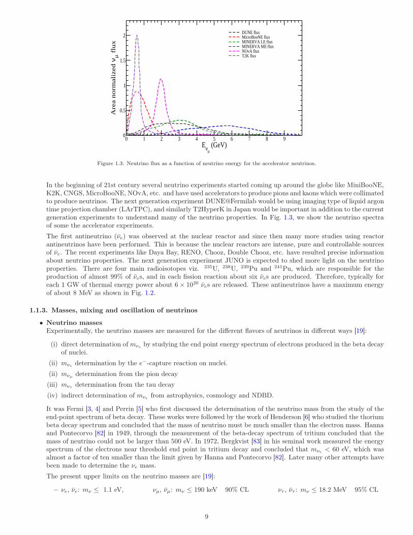
Figure 1.3: Neutrino flux as a function of neutrino energy for the accelerator neutrinos.

In the beginning of 21st century several neutrino experiments started coming up around the globe like MiniBooNE,K2K, CNGS, MicroBooNE, NOvA, etc. and have used accelerators to produce pions and kaons which were collimatedto produce neutrinos. The next generation experiment DUNE@Fermilab would be using imaging type of liquid argontime projection chamber (LArTPC), and similarly T2HyperK in Japan would be important in addition to the currentgeneration experiments to understand many of the neutrino properties. In Fig. 1.3, we show the neutrino spectraof some the accelerator experiments.

The first antineutrino (νe) was observed at the nuclear reactor and since then many more studies using reactorantineutrinos have been performed. This is because the nuclear reactors are intense, pure and controllable sourcesof νe. The recent experiments like Daya Bay, RENO, Chooz, Double Chooz, etc. have resulted precise informationabout neutrino properties. The next generation experiment JUNO is expected to shed more light on the neutrinoproperties. There are four main radioisotopes viz. 235U, 238U, 239Pu and 241Pu, which are responsible for theproduction of almost 99% of νes, and in each fission reaction about six νes are produced. Therefore, typically foreach 1 GW of thermal energy power about 6× 1020 νes are released. These antineutrinos have a maximum energyof about 8 MeV as shown in Fig. 1.2.

1.1.3. Masses, mixing and oscillation of neutrinos

• Neutrino massesExperimentally, the neutrino masses are measured for the different flavors of neutrinos in different ways [19]:

(i) direct determination of mνe by studying the end point energy spectrum of electrons produced in the beta decayof nuclei.

(ii) mνe determination by the e−-capture reaction on nuclei.

(ii) mνµ determination from the pion decay

(iii) mντ determination from the tau decay

(iv) indirect determination of mνe from astrophysics, cosmology and NDBD.

It was Fermi [3, 4] and Perrin [5] who first discussed the determination of the neutrino mass from the study of theend-point spectrum of beta decay. These works were followed by the work of Henderson [6] who studied the thoriumbeta decay spectrum and concluded that the mass of neutrino must be much smaller than the electron mass. Hannaand Pontecorvo [82] in 1949, through the measurement of the beta-decay spectrum of tritium concluded that themass of neutrino could not be larger than 500 eV. In 1972, Bergkvist [83] in his seminal work measured the energyspectrum of the electrons near threshold end point in tritium decay and concluded that mνe < 60 eV, which wasalmost a factor of ten smaller than the limit given by Hanna and Pontecorvo [82]. Later many other attempts havebeen made to determine the νe mass.

The present upper limits on the neutrino masses are [19]:

– νe, νe: mν ≤ 1.1 eV, νµ, νµ: mν ≤ 190 keV 90% CL ντ , ντ : mν ≤ 18.2 MeV 95% CL

9

• Neutrino mixing and oscillationsPontecorvo [84] in 1957 proposed the idea of neutrino oscillation by stating that the physical state of neutrinosproduced in weak interaction processes is a superposition of neutrino and antineutrino states with definite masses.This was developed in analogy with the neutral kaon regeneration phenomenon which was proposed by Gell-Mannand Pais [85], where K0 and K0 could transform into each other via weak interaction with intermediate states ofpions K0 ←→ 2π ←→ K0, K0 ←→ 3π ←→ K0, which implies that a beam that initially consists of |K0〉 pure state,would have some component of |K0〉 after some time and they propagate as the superposition of the states, |K1〉 and|K2〉, having definite masses and decay widths. Later Maki, Nakagawa and Sakata [86] applied the idea of neutrinooscillation in flavor space in which neutrino oscillation between neutrinos of two flavor i.e. νe and νµ was proposedand was later extended to three flavors of neutrinos. In the three flavor neutrino oscillation, a neutrino created ina specific flavor eigenstate is a specific quantum superposition of all three mass eigenstates. As a consequence thethree flavor of neutrinos, viz. νe, νµ, ντ , while propagating in space, travel as some admixture of three neutrinomass eigenstates viz. νi (i = 1, 2, 3) with masses mi, where the strengths of the mixing of the mass eigenstates forthe three neutrino flavors are different like νe has maximum contribution from ν1 or ντ has maximum contributionfrom ν3 mass eigenstate. The idea of neutrino mixing leading to neutrino oscillations requires the neutrino massstates to be nondegenerate and in the case of n flavor oscillation, (n− 1) neutrino mass states have nonzero masses.

The physics of neutrino mass, mixing and oscillations can be demonstrated by a simple example of two flavor mixingof νe and νµ in analogy with the quark mixing [18]. A pure νe beam described by a wave function while travellingin space may develop a component of νµ in this beam and the mixture of the νµ wave function will describe theprobability of finding νµ component in the νe beam after a time t. We assume that the flavor states νe and νµparticipating in the weak interactions are mixture of the mass eigenstates ν1 and ν2 and the mixing is described bya unitary mixing matrix U such that:

νl=e,µ =∑

i=1,2

Uliνi. (1.4)

The unitarity of the U matrix requires that in 2-dimensional space it is described by one parameter which is generallychosen to be θ such that:

U =

(

c12 s12−s12 c12

)

(1.5)

where c12 = cos θ and s12 = sin θ. As pure beam of νe at t = 0 propagates, the mass eigenstates |ν1〉 and |ν2〉,occurring in Eq. (1.4), would evolve according to

|ν1(t)〉 = ν1(0)e−iE1t; |ν2(t)〉 = ν2(0)e

−iE2t (1.6)

where E1 =√

|~p|2 +m21 ≈ |~p| +

m21

2|~p| and E2 =√

|~p|2 +m22 ≈ |~p| +

m22

2|~p| , with common momentum ~p and energies

E1 and E2. m1 and m2 are the masses of ν1 and ν2 states, respectively. After a time t, the state |νe(t)〉 will be adifferent admixture of |ν1〉 and |ν2〉. The probability of finding νµ in the beam of νe at a later time t is given by [10]:

P (νe → νµ) = sin2 2θ sin2(

∆m2

4EL

)

= sin2 θ sin2(

1.27∆m2

EL[eV2][km]

[GeV]

)

. (1.7)

Thus, we see that for P (νe → νµ) 6= 0 we need ∆m2 6= 0 and θ 6= 0 i.e. we need the mass difference between theneutrino mass eigenstates to be nonzero implying that at least one of them is massive and the mixing angle θ to benonzero. Thus, if the explanation of the solar neutrino flux deficit and other deficits observed in the atmospheric,reactor and accelerator neutrinos are explained to be due to the neutrino oscillations, the neutrinos should havenonzero mass and the neutrino flavors should mix. In the case of three flavor neutrino mixing, these flavor and masseigenstates are related by a 3× 3 unitary lepton mixing matrix [10]:

|να〉 =3∑

i=1

Uαi|νi〉 (α = e, µ, τ) , (1.8)

where U is Pontecorvo-Maki-Nakagawa-Sakata (PMNS) mixing matrix [84, 86, 87]. The most popular parameteri-zation of the PMNS matrix is given by [19]:

U =

c13c12 c13s12 s13e−iδCP

−c23s12 − s13s23c12eiδCP c23c12 − s13s23s12eiδCP c13s23s23s12 − s13c23c12eiδCP −s23c12 − s13c23s12eiδCP c13c23

(1.9)

where e.g. cij = cos θij and sij = sin θij , and δ is the CP violating phase.

10

ν(ν)-Experiment Dominant ImportantSolar θ12 ∆m2

21, θ13Reactor LBL ∆m2

21 θ12, θ13Reactor MBL θ13, |∆m2

31,32|Atmospheric θ23, |∆m2

31,32|, θ13, δCP

Accelerator LBL νµ(νµ) disappearance |∆m231,32|, θ23

Accelerator LBL νe(νe) appearance δCP θ13 , θ23

Table 1.1: Sensitivity of the (anti)neutrino sources to the oscillation parameters [19].

The general expression for the survival probability is given by [10]:

Pνα→να(L,E) = 1− 4∑

i>j

(

|Uαi|2|Uαj |2)

sin2(∆m2

ij

4EL)

. (1.10)

For the three flavors of neutrinos i, j = 1, 2, 3, with i > j, the mass squared difference terms are ∆m232, ∆m

231, and

∆m221. Since

∆m232 = m2

3 −m22 = (m2

3 −m21) + (m2

1 −m22) = ∆m2

31 −∆m221, (1.11)

therefore, only two of the three ∆ij ’s are independent.

The various experimental efforts, with the the solar, reactor, atmospheric, and accelerator neutrinos made with theshort and long baseline experiments are sensitive to the different parameters of the PMNS matrix which have beentabulated in Table-1.1.

1.1.4. Electromagnetic properties of neutrinos

Pauli in his neutrino proposal speculated that the magnetic moment of this particle should not be larger than e ×10−13cm [1]. Very soon after the discovery of antineutrinos, in 1956, Reines and Cowan [88] gave an upper limit onthe neutrino magnetic moment µνe = 10−9µB (µB is the Bohr magneton), based on the extent of nonobservation ofscintillator pulses along the path of reactor antineutrinos in their experiment. Their studies motivated Bernstein andLee [89] and many others to phenomenologically study neutrino magnetic moment.

In general, the electroweak properties of a spin 12 Dirac particle is described in terms of the two vector form factors

called the electric and the magnetic form factors, which in the static limit define the charge and the magnetic moment,and the two axial-vector form factors called the axial-vector and the tensor form factors which in the static limit definethe axial charge and the electric dipole moment, and that is related to the matrix element of the electromagnetic currentbetween the initial and final neutrino mass states [10]:

〈ψ(p′)| JEMµ |ψ(p)〉 = u(p′)

[

FQ(Q2)γµ − FM (Q2)iσµνq

ν + FE(Q2)σµνq

νγ5 + FA(Q2)(

−Q2γµ − qµq)

γ5]

u(p),

where q = p − p′, FQ(Q2), FM (Q2), FE(Q

2) and FA(Q2) are, respectively, charge, magnetic dipole, electric dipole and

axial charge neutrino electromagnetic form factors.If the neutrino is considered to be the Dirac neutrino with nonzero mass, it could have these form factors to be

nonvanishing and experimental attempts can be made to study them. In this case, they have magnetic dipole momentlike neutrons and can have electric dipole moment if CP is violated in the lepton sector. Since neutrinos participate in weakinteraction which violates CP invariance, they may have an electric dipole moment. If the neutrinos are Majorana fermionsthen from CPT invariance, regardless of whether CP invariance is violated or not, FQ(Q

2) = FM (Q2) = FE(Q2) = 0, and

only the axial-vector form factor FA(Q2) can be nonvanishing. Thus the electromagnetic properties of the (anti)neutrinos

depend upon the type of (anti)neutrinos.The SM calculations for the magnetic moment of a neutrino depends upon its mass mν and is therefore very small

of the order 3×10−19mν

eV µB. There are models where the neutrino magnetic moment is not proportional to the neutrinomass and give larger magnetic moments. Experimentally, the laboratory limits on the neutrino magnetic moments areobtained by performing the elastic νe− e, νe− e and νµ− e scattering. The present upper limits on the neutrino magneticmoments are [19]:

• µνe < 0.28× 10−10µB; µνµ < 6.8× 10−10µB; µντ < 3.9× 10−7µB 90% CL

(i) The neutrinos are assumed to be electrically neutral, but there are attempts to measure the charge of the neutrino inβ-decays by measuring the charge of the neutron Qn and the total charge of the proton and electron i.e. |Qp+Qe− |

11

in the decay n → p + e− + νe [90, 91]. This gives a limit on Qν < (0.5 ± 2.9) × 10−21e. The astrophysical limitderived from the SN1987A supernova observation is [92]:

Qν < 2× 10−15e.

(ii) The charge of neutrino is consistent with zero to a very high degree of precision but it may have a charge distributionlike a neutron. Attempts to determine the charge radius have been made [93] for νe and νµ from νee [94], νee [95]and νµe [96] scattering. Like hadrons, the mean square charge radius of a neutrino is deduced from the measurementof the vector form factor in the νee and νµe elastic scattering using the relation

〈r2〉 = 6d

dQ2F (Q2)

∣

∣

∣

∣

Q2=0

, (1.12)

where F (Q2) is the charge form factor corresponding to the matrix element of the vector current. In the case ofneutral particles, the value of 〈r2〉 could be negative or positive and the following experimental limits [19, 97, 98]are obtained in the case of νe and νµ:

−5.3× 10−32 <[

〈r2〉νµ]

< 1.3× 10−32 cm2,

−0.77× 10−32 <[

〈r2〉νµ]

< 2.5× 10−32 cm2,

−5.0× 10−32 <[

〈r2〉νe]

< 10.2× 10−32 cm2.

1.2. Theoretical description of neutrinos and their interactions

1.2.1. Dirac neutrinos

The Dirac theory of electrons formulated in 1928 [99] is conventionally used to describe the neutrinos. The Pauli’sneutrinos proposed in 1930 [1] were assumed to have a tiny mass but the later developments in the phenomenologicalstudy of neutrino interactions through the nuclear β decays and the (anti)neutrino-nucleus scattering using the Fermi orthe V −A theory of weak interactions seem to be consistent with neutrinos being massless. This did not pose any problemin applying the Dirac theory of electrons to neutrinos as the theory can be extrapolated smoothly to the massless limitof the spin 1

2 fermion of mass m → 0. These neutrinos are called Dirac neutrinos, νD, and the wave function ΨνD (x)describing these neutrinos satisfies the Dirac equation [99]:

(iγµ∂µ −m)ΨνD (x) = 0, (1.13)

where γµs (µ = 0, 1, 2, 3) are four 4× 4 matrices and satisfy the algebra:

γµ, γν = 2gµν , g00 = 1, gij = −δij (i, j = 1, 2, 3), 㵆 = γ0γµγ0. (1.14)

These relations are independent of the representation used to parameterize the γµ matrices for which many representationsexist. The most popular is the Pauli-Dirac representation in which

γ0 =

(

I 00 −I

)

, γi =

(

0 σi

−σi 0

)

,

where σi being Pauli matrices. But there are parameterizations like the Weyl, and Majorana representations, which arealso used to describe the neutrinos [10]. The wave function ΨνD in Eq. (1.13) is a four component spinor and is generallywritten as

ΨνD (x) =∑

r,p

1√

2ω~p

[

ar(p)ur(~p )e−ip·x + b†r(p)vr(~p )e

ip·x] , (1.15)

where ur(~p) and vr(~p) are the two component spinors which describe the two spin states of particles (neutrinos) andantiparticles (antineutrinos) corresponding to the spin states labeled by |s sz〉 = | 12 ± 1

2 〉 and satisfy, in the momentumspace, the equations

(

/p−m)

ur(~p) = 0;(

/p+m)

vr(~p) = 0. (1.16)

If the spin quantization axis is chosen in the direction of motion along the Z-axis, then the νD state | 12 + 12 〉 with its

spin along the +Z-axis is denoted by νD+ (right handed), while the νD state | 12 − 12 〉 has the spin opposite to Z-axis (left

handed) is denoted by νD− . Similarly, we have the two spin up and spin down states of the antineutrinos νD+ and νD− . Itshould be noted that under CPT transformation in which a particle becomes an antiparticle with opposite spin, νD− → νD+and νD+ → νD− , with the same mass. Moreover, if the neutrinos have a mass then its speed is less than the speed oflight and an observer can move faster than this speed. In this frame, an observer would see a right handed neutrino

12

νD+ as the left handed νD− but all other properties, if any, like the lepton number, etc., would be the same. In fact, νD+and νD− are the two spin states of the same particle neutrino. Similarly, νD+ and νD− are the two spin states of the sameantineutrino. There are, therefore, four states of a Dirac neutrino, described by ΨνD . The phenomenological study of theweak interaction processes involving (anti)neutrinos establishes that for each flavor of neutrinos [10]:

(i) the neutrinos are left handed i.e. νD− and the antineutrinos are right handed i.e. νD+ , which take part in the weakinteractions.

(ii) νD− always produces a charged lepton l− and νD+ always produces a charged lepton l+ in charged current (CC)interactions, which imply that νD− and νD+ are distinct particles.

To ensure that νD− and νD+ are distinct particles like l− and l+ and obey the selection rules of weak processes, itwas proposed that

1. there exists a new quantum number called lepton number Ll for each flavor l and (νDl− l−) were assigned

Ll = +1 while (νDl+ l+) were assigned Ll = −1.2. The lepton number Ll is conserved for each flavor.

(iii) While the charged leptons and their antiparticles like l− and l+ are different in their charge and lepton number, thecorresponding neutrinos and antineutrinos being neutral are different only in their lepton number Ll and helicities.It should be noted that νDl+ and νDl− have the same lepton number Ll = +1. Similarly, νDl+ and νDl− also have thesame lepton number Ll = −1.

1.2.2. Weyl neutrinos

In the limit of mass m→ 0, interesting features arise which become more intriguing in the case of neutrinos being neutralparticles. In this limit, the Dirac equation becomes Weyl equation and the Weyl wave function ΨνW satisfies

iγµ∂µΨνW (x) = 0. (1.17)

This equation of motion for a spin 12 particle with m = 0 was especially studied by Weyl in 1929 [100], a year after the

Dirac equation [99], and is most easily solved using the Weyl representation for the γ matrices [100].

However, we discuss its solution using the chirality operator which is defined as γ5 = iγ0γ1γ2γ3 =

(

0 I

I 0

)

for the

following reason. Using the 4-dimensional representation of spin ~Σ =

(

~σ 00 ~σ

)

= γ5γ0~γ, the helicity operator ~Σ · p is

written as ~Σ · p = γ5γ0~γ · p. In the case of m→ 0, the Weyl equation is written, in momentum space, as

/p ΨνW (p) = 0. (1.18)

Now, consider the equation~Σ · ~p ΨνW (p) = γ5γ0~γ · ~p ΨνW (p). (1.19)

Using p0 = |~p | and Eq. (1.18) in the case of m = 0, we get

~Σ · p ΨνW (p) = γ5 ΨνW (p). (1.20)

Thus, in the case of m = 0, γ5 is the helicity operator ~Σ · p, which is also called the chirality operator. Since ~Σ · p ~Σ · p ≡(γ5)2 = 1, γ5 has two eigenvalues ±1 corresponding to helicity +1 and −1, also called the right handed (R) and lefthanded (L) helicity states of the massless neutrino. The eigen functions corresponding to the eigenvalues +1 and −1 are,respectively, ΨW

R and ΨWL , which satisfy

~Σ · p ΨWR (p) = γ5 ΨW

R (p) = (+1) ΨWR (p), ~Σ · p ΨW

L (p) = γ5 ΨWL (p) = (−1) ΨW

L (p). (1.21)

It should be noted that in m→ 0, νWR and νWL are two distinct particles and not the two spin states of one particle as inthe case of the Dirac neutrinos νD+ and νD− (in the case of m 6= 0) because there exists no frame in which νWR would appearas νWL due to the Weyl neutrinos moving with the speed of light. In principle, while νD+ and νD− have the same leptonnumber, νWR and νWL could have different lepton numbers. If neutrinos exist in νWL state, then they cannot exist in νWRstate. Consequently, the antineutrinos will exist in νWR state and not in νWL state. Thus, the Weyl (anti)neutrinos haveonly those states unlike the Dirac (anti)neutrinos which have four states. If physical neutrinos observed in nuclear β decaysor other weak processes are νWL (or νWR ), the massless Weyl neutrinos imply maximal violation of the left-right symmetryi.e., parity violation. This is the reason that the Weyl equation was disfavored during 1930–1957. After the parityviolation was proposed and observed experimentally [16], the two component theory of neutrinos with chiral invariance

13

was proposed by Lee and Yang [101], Landau [102], and Salam [103]. If the two states νWL and νWR are independent, inthe case of m = 0, then we can write a neutrino state νW as

ΨW = ΨWL +ΨW

R . (1.22)

Using Eqs. (1.21) and (1.22), we obtain

ΨWL =

I− γ52

ΨW , ΨWR =

I+ γ52

ΨW , (1.23)

as the left-handed and right-handed Weyl neutrinos. Conversely, if νW exists either in νWL or in νWR state, it has to bemassless as the mass term in the Lagrangian given by

LWmass = −mΨWΨW = −m(

ΨWL ΨW

R + ΨWR ΨW

L

)

(1.24)

vanishes.The V − A theory of weak interaction was formulated using the two component neutrinos by Sudarshan and Mar-

shak [11], and Feynman and Gell-Mann [12] using left handed neutrinos νWL . The antineutrino in the Weyl theory areobtained in a similar manner by performing a CPT transformation such that

νWRCPT−−−→ νWL , νWL

CPT−−−→ νWR . (1.25)

The relation between the Dirac and Weyl neutrinos can be expressed as

(i) Four component Dirac spinor is equivalent to two two-component Weyl spinors.

(ii) While Dirac neutrinos could have nonvanishing mass (m) and can be extrapolated to m → 0, Weyl neutrinos arenecessarily massless.

(iii) νD+(−)

m→0−−−→ νWR(L); νD+(−)

m→0−−−→ νWR(L).

1.2.3. Majorana neutrinos

While the phenomenology of the weak interaction processes was consistent with the massless neutrinos, the experimentalattempts to measure their masses were continuing relentlessly. Theoretically also the mass of νe(νe) was being inferredfrom the experimental observations made in astrophysics and cosmology. The improvements in the experimental limits ofthe neutrino masses of various flavors are reported periodically and a nonzero mass for neutrino is not ruled out. However,the observation of neutrino oscillations involving all the three flavors of neutrinos νe, νµ and ντ in the experiments withsolar, reactor, atmospheric, and accelerator neutrinos, confirmed that the neutrinos (at least two flavors) have masseseven though very small. This rules out the neutrinos being Weyl neutrinos. However, the neutrinos being neutral particlescould be still described by a two component neutrino, if they are their own antiparticles. Such a possibility was studiedby Majorana in his celebrated paper on “The symmetry of the theory of electrons and positrons” [104]. These neutrinosare called Majorana neutrinos νM . If the Majorana neutrino is its own antiparticle, then its wave function described byΨνM (x) satisfies the equation

ΨνM (x) = Ψ⋆νM (x) (1.26)

implying that ΨνM (x) is real. But the wave function of the neutrinos written in Eq. (1.13) or Eq. (1.26) is complex dueto some of the coefficients γµ being complex. If a representation could be found in which all the γµ’s are imaginary suchthat the coefficients (iγµ∂

µ −m) are real, then the solutions Ψν(x) and Eq. (1.26) would be satisfied. This was done byMajorana by using Majorana representation of the gamma matrices, in which γµ’s are defined as:

γ0 =

(

0 σ2σ2 0

)

, γ1 =

(

iσ3 00 iσ3

)

, γ2 =

(

0 −σ2σ2 0

)

, γ3 =

(

−iσ1 00 −iσ1

)

,

and γ5 = iγ0γ1γ2γ3 =

(

σ2 00 −σ2

)

, and all of them are purely imaginary. This Majorana representation γµ of Dirac

matrices satisfy the algebra of Dirac matrices given in Eq. (1.14). However, Eq. (1.26) is not covariant i.e. if this equationis satisfied in Majorana representation in one Lorentz frame, it will not be satisfied in another Lorentz frame as theLorentz transformation of spinors depend on γµ matrices which change in another frame. For making this equation validin other frames a conjugate field Ψc

ν(x) is defined as

Ψcν(x) = Cγ0Ψ∗

ν(x), (1.27)

14

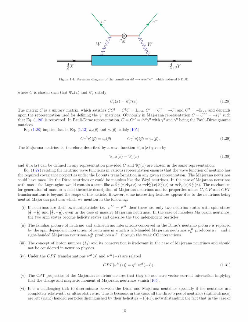
e− e−

νMW−W−

AZX

AZ+2Y

Figure 1.4: Feynman diagram of the transition dd −→ uue−e−, which induced NDBD.

where C is chosen such that Ψν(x) and Ψcν satisfy

Ψcν(x) = Ψc∗

ν (x). (1.28)

The matrix C is a unitary matrix, which satisfies CC† = C†C = I4×4, CT = C† = −C, and C2 = −I4×4 and depends

upon the representation used for defining the γµ matrices. Obviously in Majorana representation C = CM = −iγ0 suchthat Eq. (1.28) is recovered. In Pauli-Dirac representation, C = CD = iγ2γ0 with γ2 and γ0 being the Pauli-Dirac gammamatrices.

Eq. (1.28) implies that in Eq. (1.13) ur(~p) and vr(~p) satisfy [105]

Cγ0v∗r (~p) = vr(~p) Cγ0u∗r(~p) = ur(~p). (1.29)

The Majorana neutrino is, therefore, described by a wave function ΨνM (x) given by

ΨνM (x) = Ψcν(x) (1.30)

and ΨνM (x) can be defined in any representation provided C and Ψ∗ν(x) are chosen in the same representation.

Eq. (1.27) relating the neutrino wave functions in various representation ensures that the wave function of neutrino hasthe required covariance properties under the Lorentz transformation in any given representation. The Majorana neutrinoscould have mass like the Dirac neutrinos or could be massless like the Weyl neutrinos. In the case of Majorana neutrinoswith mass, the Lagrangian would contain a term like mΨC

ν (x)Ψν(x) or mΨCν (x)Ψ

Cν (x) or mΨν(x)Ψ

Cν (x). The mechanism

for generation of mass or a field theoretic description of Majorana neutrinos and its properties under C, CP and CPTtransformations is beyond the scope of this article. However, some interesting features appear due to the neutrinos beingneutral Majorana particles which we mention in the following:

(i) If neutrinos are their own antiparticles i.e. νM = νM then there are only two neutrino states with spin states| 12 ,+ 1

2 〉 and | 12 ,− 12 〉, even in the case of massive Majorana neutrinos. In the case of massless Majorana neutrinos,

the two spin states become helicity states and describe the two independent particles.

(ii) The familiar picture of neutrino and antineutrino interactions conceived in the Dirac’s neutrino picture is replacedby the spin dependent interaction of neutrinos in which a left-handed Majorana neutrinos νML produces a l− and aright-handed Majorana neutrinos νMR produces a l+ through the weak CC interactions.

(iii) The concept of lepton number (Ll) and its conservation is irrelevant in the case of Majorana neutrinos and shouldnot be considered in neutrino physics.

(iv) Under the CPT transformations νM (s) and νM (−s) are related

CPT |νM (s)〉 = ηs |νM (−s)〉 . (1.31)

(v) The CPT properties of the Majorana neutrino ensures that they do not have vector current interaction implyingthat the charge and magnetic moment of Majorana neutrinos vanish [105].

(vi) It is a challenging task to discriminate between the Dirac and Majorana neutrinos specially if the neutrinos arecompletely relativistic or ultrarelativistic. This is because, in this case, all the three types of neutrinos (antineutrinos)are left (right) handed particles distinguished by their helicities −1(+1), notwithstanding the fact that in the case of

15

Dirac and Weyl neutrinos (antineutrinos) they are also distinguished by an additional quantum number, i.e., leptonnumber.

There is extensive discussion of various processes, in which there is a possibility to distinguish between the Dirac andthe Majorana neutrinos [106, 107]. However, the most distinct process which establishes the existence of Majorananeutrinos is the process of NDBD of nuclei in which the νe produced in the process n −→ p+ e− + νe is absorbedby another neutron i.e. n + νe(= νe) −→ e− + p such that n + n −→ p + p + e− + e− in the nucleus leading toAZX −→A

Z+2 Y +e−+e− as shown in Fig. 1.4. These processes were discussed by Racah [108] and Furry [109, 110] soonafter Majorana’s theory. In Fig. 1.4, ⊗ denotes the neutrino interaction in the Majorana mass term, which changesthe helicity of the neutrino. Such an interaction requires the Majorana neutrino to have mass or the presence of righthanded currents. Various theoretical models have been used to calculate NDBD using BSM physics. Experimentally,there are enormous efforts being made to observe such nuclear decays in various experiments being done around theworld, for example, EXO-200, KamLAND-Zen, NEMO-3, CUORE, ELEGANT-IV, GERDA, etc. For a review, seeRef. [111].

In this work, we focus on the neutrino interactions with matter using the SM. The SM is presented briefly in the followingSection.

1.3. Standard model of electroweak interactions

1.3.1. Introduction

The SM was formulated by Weinberg [20] and Salam [21] as the theory of the electroweak interaction of leptons. Itwas extended to the quark sector using the Glashow, Illiopolis and Maiani [22] scheme of quark mixing proposed earlierby Cabibbo [17]. The formulation of SM makes use of the experimental results on the properties and interactions ofneutrinos obtained from the phenomenological V −A theory of weak interactions and the theoretical ideas from the localgauge field theories based on the invariance under continuous symmetry, to generate the interactions. Such gauge fieldtheories, require the existence of massless vector bosons known as Nambu-Goldstone bosons which mediate the interactionbetween the matter fields describing the physical particles in field theories. This mechanism of generating interactions,works in the case of electromagnetic interactions where the invariance of the Lagrangian describing the charged leptonsl(= e, µ, τ) under the local gauge U(1) symmetry, generates a massless vector field Aµ(x), which is identified as theelectromagnetic field and mediates the electromagnetic interaction between charged particles. However, this mechanismis not sufficient to generate CC weak interactions, which are mediated by the two massive vector fields Wµ+(x) andWµ−(x). Consequently, a symmetry group higher than U(1), which can generate more than one vector field and includesa mechanism to generate masses of the vector fields is needed. In the SM proposed by Weinberg [20] and Salam [21],a higher group SU(2)IW × U(1)YW

(where IW and YW are the isospin and hypercharge operators in weak interactionsdefined in analogy with the strong interactions), is considered, which requires the existence of four massless vector fields,when the invariance under this symmetry is imposed on the Lagrangian. The masses of three of these vector fields leavingone field massless are generated using the mechanism of spontaneous breaking of symmetry proposed by Englert andBrout [24], and Higgs [25] by introducing a doublet of interacting scalar fields φ+(x) and φ0(x) in the theory. The twoout of the three massive fields are identified as Wµ+(x) and Wµ−(x) fields, mediating the CC weak interactions and thethird massive field is the neutral vector field Zµ, which is new and is predicted to mediate NC interactions in the weaksector. The massless field Aµ(x) is identified as the electromagnetic field. The SM was shown later, to be renormalizableby ’t Hooft and Veltman [26] and Lee and Zinn-Justin [27].

For a review of the local gauge field theories based on the continuous symmetries, implying the existence of masslessNambu-Goldstone bosons and the phenomenon of Higgs mechanism to generate the masses of the Nambu-Goldstonebosons and the renormalizability of the SM, the reader is referred to a general text on quantum field theory [112].

1.3.2. SM of electroweak interaction of leptons

The essential results about the neutrino properties and their interactions obtained from the phenomenological V − Atheory used in formulating the SM are summarized as:

(i) the (anti)neutrinos are considered to be neutral, massless, left-handed spin 12 particles with helicity −1(+1) which

exist in three flavors of neutrinos i.e. νl = νe, νµ, ντ and their antiparticles.

(ii) the (anti)neutrino of each flavor l are assigned a lepton number Ll = +1(−1), which is conserved in weak interactions.

(iii) the neutrinos of flavor l(= e, µ, τ) interact with other leptons through the interaction of leptonic currents lµ(x),which has V −A structure defined as

lµ(x) =∑

l=e,µ,τ

Ψl(x)γµ(1− γ5)Ψνl(x) (1.32)

16

νe(νe)

e−(e+)

W±

νµ(νµ)

µ−(µ+)

W±

ντ (ντ )

τ−(τ+)

W±

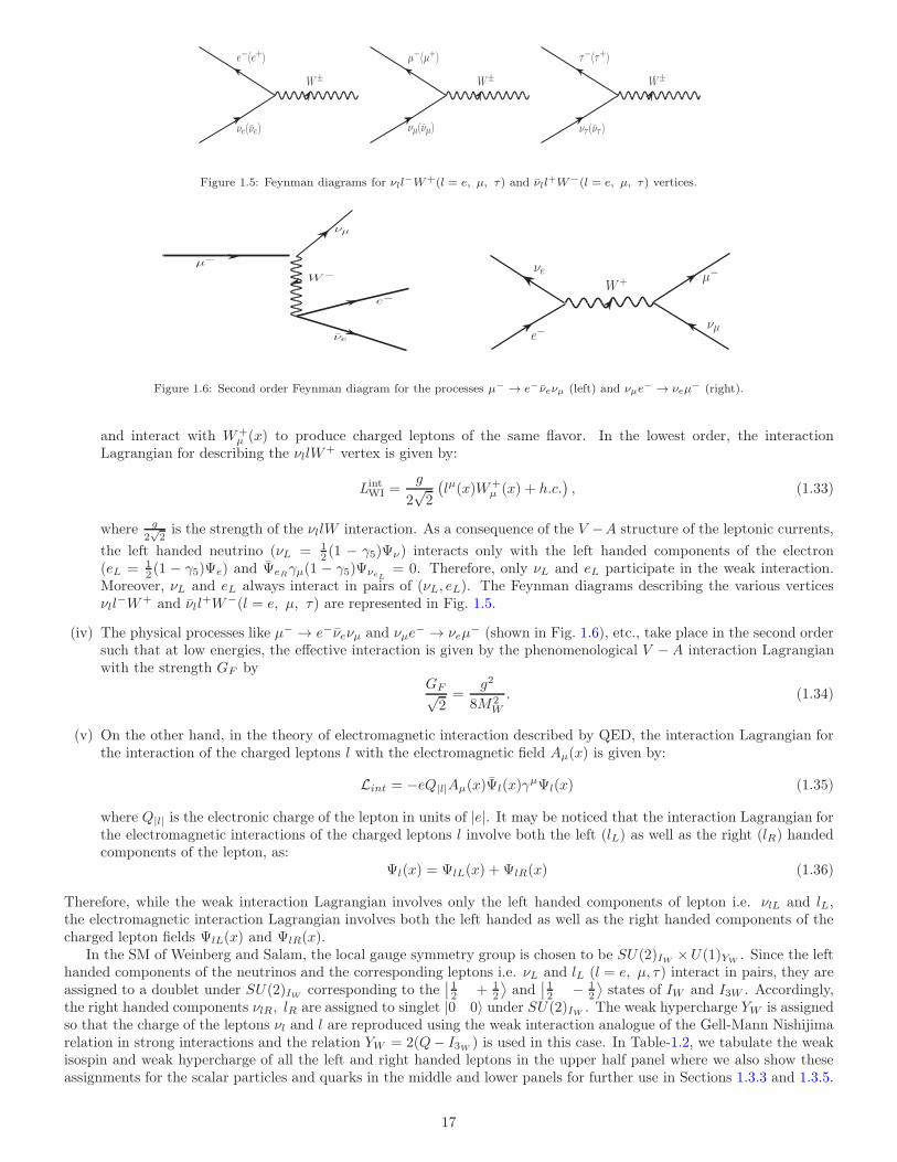
Figure 1.5: Feynman diagrams for νll−W+(l = e, µ, τ) and νll

+W−(l = e, µ, τ) vertices.

µ−

νµ

W−

e−

νe

νe

e−

W+ µ−

νµ

Figure 1.6: Second order Feynman diagram for the processes µ− → e−νeνµ (left) and νµe− → νeµ− (right).

and interact with W+µ (x) to produce charged leptons of the same flavor. In the lowest order, the interaction

Lagrangian for describing the νllW+ vertex is given by:

LintWI =

g

2√2

(

lµ(x)W+µ (x) + h.c.

)

, (1.33)

where g

2√2

is the strength of the νllW interaction. As a consequence of the V −A structure of the leptonic currents,

the left handed neutrino (νL = 12 (1 − γ5)Ψν) interacts only with the left handed components of the electron

(eL = 12 (1 − γ5)Ψe) and ΨeRγµ(1 − γ5)ΨνeL

= 0. Therefore, only νL and eL participate in the weak interaction.Moreover, νL and eL always interact in pairs of (νL, eL). The Feynman diagrams describing the various verticesνll

−W+ and νll+W−(l = e, µ, τ) are represented in Fig. 1.5.

(iv) The physical processes like µ− → e−νeνµ and νµe− → νeµ

− (shown in Fig. 1.6), etc., take place in the second ordersuch that at low energies, the effective interaction is given by the phenomenological V −A interaction Lagrangianwith the strength GF by

GF√2=

g2

8M2W

. (1.34)

(v) On the other hand, in the theory of electromagnetic interaction described by QED, the interaction Lagrangian forthe interaction of the charged leptons l with the electromagnetic field Aµ(x) is given by:

Lint = −eQ|l|Aµ(x)Ψl(x)γµΨl(x) (1.35)

where Q|l| is the electronic charge of the lepton in units of |e|. It may be noticed that the interaction Lagrangian forthe electromagnetic interactions of the charged leptons l involve both the left (lL) as well as the right (lR) handedcomponents of the lepton, as:

Ψl(x) = ΨlL(x) + ΨlR(x) (1.36)

Therefore, while the weak interaction Lagrangian involves only the left handed components of lepton i.e. νlL and lL,the electromagnetic interaction Lagrangian involves both the left handed as well as the right handed components of thecharged lepton fields ΨlL(x) and ΨlR(x).

In the SM of Weinberg and Salam, the local gauge symmetry group is chosen to be SU(2)IW ×U(1)YW. Since the left

handed components of the neutrinos and the corresponding leptons i.e. νL and lL (l = e, µ, τ) interact in pairs, they areassigned to a doublet under SU(2)IW corresponding to the

∣

∣

12 + 1

2

⟩

and∣

∣

12 − 1

2

⟩

states of IW and I3W . Accordingly,the right handed components νlR, lR are assigned to singlet |0 0〉 under SU(2)IW . The weak hypercharge YW is assignedso that the charge of the leptons νl and l are reproduced using the weak interaction analogue of the Gell-Mann Nishijimarelation in strong interactions and the relation YW = 2(Q− I3W ) is used in this case. In Table-1.2, we tabulate the weakisospin and weak hypercharge of all the left and right handed leptons in the upper half panel where we also show theseassignments for the scalar particles and quarks in the middle and lower panels for further use in Sections 1.3.3 and 1.3.5.

17

In the following, we summarize the main steps in formulating the SM for leptons and for simplicity consider the case ofνe and e− which can be generalized to other flavors of leptons. We introduce the notation ΨL(x) and ΨR(x) to representthe doublet state of the left handed component of leptons (νL, eL) and the singlet state of the right handed componentof the leptons νR and eR as:

ΨL =

(

Ψνe

Ψe

)

L

=

(

νLeL

)

, ΨeR = eR, ΨνeR= νeR (1.37)

where ΨL = 12 (1− γ5)Ψ, with Ψ =

(

Ψνe

Ψe

)

, ΨeR = 12 (1 + γ5)Ψe and ΨνR = 1

2 (1 + γ5)Ψνe .

A Lagrangian for the free massless leptons νL, eL and eR is written as

L =∑

j=L,eR,νR

Ψj /∂Ψj(x) (1.38)

with /∂ = γµ ∂∂xµ

. The Lagrangian is invariant under the transformations of the global symmetry group SU(2)IW ×U(1)YW

generated by the gauge transformations U = U1U2, where U1 = ei~α·~τ2 , U2 = eiβI , and ~α(α1, α2, α3) and β are the

parameters describing the transformation of U1 and U2, respectively, and τ1 =

(

0 11 0

)

, τ2 =

(

0 −ii 0

)

and τ3 =

(

1 00 −1

)

are the Pauli matrices, I is the unit matrix. A mass term like mΨjΨj (= ΨjLΨjR + ΨjRΨjL) is not included as it is notinvariant under global SU(2)IW × U(1)YW

. However, when the transformations are made local by replacing ~α → ~α(x)and β → β(x) then the Lagrangian given in Eq. (1.38) is not invariant under the local gauge group generated by thelocal gauge transformations U1(x)U2(x) due to the presence of the derivation term ∂

∂xµin the Lagrangian. In order to

restore the invariance of the Lagrangian under local transformation, the Lagrangian is rewritten in terms of the covariant

derivative DDxµ instead of the ordinary derivative ∂

∂xµ by introducing the matrix valued gauge fields Wµ =∑

iτ i

2 ·Wµi

corresponding to U1(x) and the field Bµ corresponding to U2(x) transformation of SU(2)IW and U(1)YWand defining

the covariant derivative DDxµ as

D

Dxµ=

∂

∂xµ+ ig

~τ · ~Wµ

2+ i

g′

2YWBµ(x), (1.39)

g and g′ being the coupling constant corresponding to SU(2)IW and U(1)YWgauge fields. A factor of 1

2 is introduced

with the Bµ(x) field in analogy with the ~Wµ(x). Requiring that the new gauge vector field Wµ and Bµ transform underU1(x) and U2(x) as:

~Wµ(x)→ ~W ′µ(x) = ~Wµ(x)− ~α× ~Wµ − i

g∂µ~α, Bµ(x)→ B′µ(x) = Bµ(x) − i

g′∂µβ(x) (1.40)

ensures that under the local gauge transformation

Ψ(x)→ Ψ′(x) = UΨ(x), DΨ(x)→ (DΨ)′(x) = U(DΨ(x)) (1.41)

making the redefined Lagrangian invariant under the local gauge transformations U(x). It can be shown using Eq. (1.39),that

[Dµ, Dν ] =g

2~τ · ~Gµν(x) +

g′

2YWBµν(x) (1.42)

where Bµν and ~Gµν being the field tensors for Bµ(x) and ~Wµ(x) fields given by:

Bµν = ∂µBν(x) − ∂νBµ(x), ~Gµν(x) = ∂µ ~W ν(x) − ∂ν ~Wµ(x) + g ~Wµ(x)× ~W ν(x). (1.43)

and are used to define the kinetic energy of the vector Bµ and ~Wµ fields.Consequently, the free particle Lagrangian is redefined as

L =∑

j=L,eR,νR

Ψj(x) /DΨj (1.44)

Writing the expressions for DµΨL, DµΨeR and DµΨνR , using the values of YW for ΨL, ΨeR and ΨνR given in Table.1.2,we obtain

DµΨL(x) =

(

∂µ +ig

2~τ · ~Wµ(x)− ig′

2Bµ(x)

)

ΨL, DµΨeR(x) = (∂µ − ig′Bµ(x))ΨR, DµΨνR = ∂µΨνR (1.45)

18

The Lagrangian in Eq. (1.44) is expanded over j and is written as

L = L0 + Lint, with

L0 = iΨL /∂ΨL + iΨeR /∂ΨeR + iΨνR /∂ΨνR , and

Lint = − g

2√2

(

νeγµ(1− γ5)eW+

µ + eγµ(1 − γ5)νeW−µ

)

−√

g2 + g′2

2νLγ

µνLZµ

+gg′

√

g2 + g′2eγµeAµ +

1√

g2 + g′2

[

−g′2eRγµeR +g2 − g′2

2eLγ

µeL

]

Zµ, (1.46)

where

W±µ =

W 1µ ∓ iW 2

µ√2

, Zµ =gW 3

µ − g′Bµ√

g2 + g′2and Aµ =

g′W 3µ + gBµ

√

g2 + g′2, (1.47)

We can observe from L that

(i) no terms like Wµi Wiµ and BµBµ (or equivalently like AµAµ, ZµZµ or W±µW∓

µ ) appear in L, implying that all thefields W+µ, W−µ, Zµ and Aµ are massless.

(ii) Lint correctly reproduces

1. CC weak interaction of νe and e with strength g

2√2

given by

LCCint = − g

2√2Ψνe

γµ(1− γ5)ΨeW+µ + h.c. (1.48)

2. the electromagnetic interaction of electrons with the electromagnetic coupling is given by

LEMint =

gg′√

g2 + g′2Ψeγ

µΨeAµ. (1.49)

(iii) Lint predicts

1. NC interaction of neutrinos is given by:

LνNC = −√

g2 + g′2

4Ψνγµ(1 − γ5)ΨνZ

µ, with strength

√

g2 + g′2

2. (1.50)

2. NC interaction of electrons is given by:

LeNC = − Zµ

√

g2 + g′2

[

g2 − g′24

Ψeγµ(1 − γ5)Ψe −g′2

2Ψeγµ(1 + γ5)Ψe

]

. (1.51)

(iv) The SM therefore describes the electroweak interaction of leptons in terms of the two parameters g and g′. ComparingLCCint and LEM

int given in Eqs. (1.48) and (1.49), respectively, with the V − A theory of weak interactions andQED of the charged leptons, we see that g and g′ are related with the strength of Fermi interaction GF and theelectromagnetic coupling e through the relations

GF√2=

g2

8M2W

,1

e2=

1

g2+

1

g′2, (1.52)

where MW is the mass of Wµ(±) vector fields.

(v) The Lagrangian obtained using the local gauge field theory, thus, predicts the electromagnetic and weak interactionsmediated by four vector gauge fields, Wµ+(x), Wµ−(x), Zµ(x) and Aµ(x), all being massless as there are no massterms like M2

V Vµi Viµ(Vi = W+,W−, Z,A) for any of the fields. While the model can describe the electromagnetic

interaction, it can not describe the weak interaction which is mediated by massive vector fields Wµ±. Therefore, themodel in this form is inconsistent with the phenomenological V −A theory of weak interactions unless a mechanismin devised to generate the masses of these fields. This is done using the Higgs mechanism.

Since all the fields Wµ+, Wµ

−, Zµ, and Aµ are massless, the kinetic energy terms are added by hand to redefine the freeLagrangian L0 as

L0 → L0 −1

4BµBµ −

1

4GµνGµν

in analogy with the kinetic energy term for massless electromagnetic field Aµ in QED.

19

1.3.3. Higgs mechanism and generation of mass

The phenomenon of spontaneous breaking of continuous symmetry in field theory proposed by Englert and Brout [24]and Higgs [25], generally called the Higgs mechanism was used by Weinberg [20] and Salam [21] to generate the massof the gauge vector bosons. In this phenomenon, strongly interacting doublet of scalar fields φ(x) are introduced in theLagrangian. The vacuum state of this Lagrangian breaks the symmetry while the Lagrangian respects the symmetry.Hence, the name spontaneous breaking of symmetry instead of the explicit breaking of symmetry in field theory is givento this phenomenon. In local gauge field theories the invariance of the Lagrangian generates massless vector gaugefields corresponding to each generator of the symmetry. In the SM, the spontaneous breaking of symmetry based onSU(2)IW × U(1)YW

, is realized by introducing interacting scalar fields φ(x) which transform as doublet under SU(2)IWi.e.

φ(x) =

(

φ+(x)φ0(x)

)

=1√2

(

φ1(x) + iφ2(x)φ3(x) + iφ4(x)

)

(1.53)

with fields φ+(x) and φ0(x) having I = 12 and I3 = ± 1

2 and are assigned YW = +1 to reproduce their charges as shownin Table-1.2 (middle panel). The interaction Lagrangian for the scalar fields φ is written in a locally gauge invariant wayunder the SU(2)IW × U(1)YW

transformation using the covariant derivative Dµ given by:

Dµφ = (∂µ + ig~τ · ~Wµ + ig′

2YWBµ)φ (1.54)

and is written as:Lφ = Dµφ†Dµφ− V (φ∗φ) (1.55)

where the potential V (φ∗φ) is given by:

V (φ∗φ) = −µ2φ∗(x)φ(x) + λ(φ∗φ)2 (1.56)

and has minimum value given by the condition:

∂V

∂φ∗= φ(x)(−µ2 + 2λφ∗φ) = 0 (1.57)

which implies that for µ2 < 0, the minimum occurs at φ(x) = 0, but for µ2 > 0, there is minima at φ†(x)φ(x) = µ2

2λ . While

φ(x) = 0 is a trivial ground state, φ†(x)φ(x) = µ2

2λ implies an infinitely degenerate value to φ(x) since it is a complex fieldgiven by φ(x) = eiθφ(x), θ being arbitrary.

The SU(2)IW × U(1)YWsymmetry is spontaneously broken in the SM by choosing:

φ1(x) = φ2(x) = φ4(x) = 0, φ3(x) 6= 0

such that vacuum expectation value (VEV) of φ(x) is given by:

〈0|φ(x) |0〉 =(

0v√2

)

, v =1√2〈0|φ3(x) |0〉 (1.58)

This choice of ground state ensures that the ground state φ0(x) remains invariant under the symmetry group transforma-tions of U(1)Q, where Q = 1

2τ3+Y2 is the generator of the group because Q |φ0〉 = 0. This means that SU(2)IW ×U(1)YW

is spontaneously broken to U(1)Q, keeping the gauge fields corresponding to U(1)Q symmetry i.e. the electromagneticfield, massless while generating the mass corresponding to other three generators τ+, τ− and 1

2 (τ3−Y ). The Lagrangianfor the Higgs field φ(x), invariant under the local gauge group SU(2)IW × U(1)IW , written in terms of the covariantderivative Dµφ given in Eq. (1.54) is written explicitly using the value of YW for φ from Table-1.2 (middle panel) as

Lφ =

(

∂µ + ig

2~τ · ~Wµ + i

g′

2Bµ

)

φ∗(x)

(

∂µ + ig

2~τ · ~Wµ + i

g′

2Bµ

)

φ(x) − V (φ∗(x)φ(x)) (1.59)

Expanding the field φ(x) around its VEV 〈φ(x)〉0 given in Eq. (1.58), and writing

φ(x) =1√2

(

0v +H(x)

)

, (1.60)

we write

Lφ =1

2∂µH(x)∂µH(x) +

v2g2

8(|W+

µ |2 + |W−µ |2) +

g2

8(H2 + 2Hv)(|W+

µ |2 + |W−µ |2) +

(

g2 + g′2

4

)(

H2 + 2Hv + v2

2

)

× ZµZµ +

[

g2g′2

4(g2 + g′2)(H2 + 2Hv)− g2g′2

4(g2 + g′2)(H2 + 2Hv)

]

AµAµ − V (φ∗(x)φ(x)). (1.61)

20

The above Lagrangian predicts the masses of the vector gauge bosons W+µ, W−µ, Zµ, where Zµ =gW 3

µ−g′Bµ√g2+g′2

and

Aµ =g′W 3

µ+gBµ√g2+g′2

to obtain

MW+ =MW− =vg

2; MZ =

v√

g2 + g′2

2; MA = 0, (1.62)

and mass of the Higgs scalar H(x) is predicted by expanding V (φ∗(x)φ(x)) using Eq. (1.60) to obtain:

MH =√2λv (1.63)

The interaction of the Higgs field H(x) with the gauge vector fields Wµ±, Zµ and Aµ given in the last two lines ofEq. (1.61). We see that the mass of Zµ and Wµ vector fields are related by

MZ

MW=

√

(

1 +g′2

g2

)

> 1 (1.64)

and the absolute values of MW and MZ are determined by g , g′, and v.

1.3.4. Neutral current interactions and the weak mixing angle

It has been shown by Eqs. (1.48) and (1.49) that the SM reproduces CC weak and electromagnetic interactions of leptons

mediated by Wµ± vector bosons with mass MW = vg2 and the massless electromagnetic vector field ~Aµ, as well as predicts

NC weak interactions for the neutrinos and electrons which are mediated by the neutral vector bosons Zµ with mass

MZ = MW

√

1 + g′2

g2 , as shown by the Eq. (1.64). The NC weak interaction is alternatively defined in terms of a weak

mixing angle θW defined as

tan θW =g′

gsuch that

MW =MZ cos θW ; e = g sin θW = g′ cos θW (1.65)

Zµ = cos θWWµ3 − sin θWBµ; Aµ = sin θWWµ

3 + cos θWBµ. (1.66)

The weak mixing angle θW mixes the neutral gauge vector bosons Wµ3 and Bµ corresponding to the SU(2)IW and U(1)YW

gauge bosons to produce the physical gauge vector fields Zµ and Aµ responsible for the weak NC and the electromagneticcurrent carrying vector fields. In terms of the weak mixing angle, the Lagrangians for the weak CC and NC interactionswritten in Eq. (1.46) are rewritten as:

LCC = − g

2√2

[

νeγµ(1− γ5)eW+

µ + h.c.]

, (1.67)

LNC = − g

2 cos θW[νeγ

µ(1− γ5)νe + eγµ(geV − geAγ5)e]Zµ, (1.68)

LEM = −|e|eγµeAµ (1.69)

where

geV = 2 sin2 θW −1

2, gνV =

1

2, geA = −1

2, gνA = −1

2. (1.70)

1.3.5. Extension of the SM to the leptons, quarks and nucleons

The extension of the SM to the leptons of other flavors is straight forward. The left and right handed components of(νµ, µ

−) and (ντ , τ−) are assigned to the SU(2)IW × U(1)YW

representations in same way as done for the (νe, e−)

leptons and shown in Table-1.2 and interaction can be generated following the procedure in Section 1.3.2 with implicitassumptions of LFU and the interactions for all the flavors of leptons can be written as:

LCC = − g

2√2

∑

l=e,µ,τ

[

νlγµ(1 − γ5)lW+

µ + h.c.]

, (1.71)

LNC = − g

2 cosθW

∑

l=e,µ,τ

[

νlγµ(1− γ5)νl + lγµ(glV − glAγ5)l

]

Zµ, (1.72)

with geV and geA given in Eq. (1.70), and have the same values for all the lepton flavors l.

21

However, the formalism presented in Section 1.3.2 can be reformulated in terms of the weak isospin (~τf ) and thecharge operators Qf for the fermions f instead of the weak hypercharge. The weak CC and NC currents are writtenusing SU(2)IY doublets, ΨfL = 1−γ5

2 Ψf and ΨfR = 1+γ5

2 Ψf for a fermion f , so that they can be applied to a lepton andquark in a unified way.

It is straight forward to see that the weak CC interaction Lagrangian is given by:

LCC =g

2√2

∑

f=e,µ,τ

Ψνfγµ(1− γ5)ΨfW

+µ + h.c. (1.73)

The weak NC Lagrangian using Eq. (1.72) is written as:

LNC = −∑

f=e,µ,τ

[

ΨfL

(

gτf32/W

3+ g′

Y fL

2/B

)

ΨfL + ΨfRg′Y

fR

2/BΨfR

]

(1.74)

where τf3 is isospin operator and Y fL and Y f

R are the hypercharges of the left- and right- handed fermions in Table-1.2.Since, τ3ΨfR = 0 as ΨfR is isosinglet, the two terms in Eq. (1.74) are combined to write:

LNC = −∑

f=e.µ,τ

∑

i=L,R

Ψfi

(

gτfi32

/W3+ g′

Y fi

2/B

)

Ψfi (1.75)

Using Eq. (1.66) to express W 3µ and Bµ in terms of Zµ and Aµ and Ψfi = 2Qfi − τfi3 , LNC can be expressed as:

LNC = − g

2 cos θW

∑

f=e,µ,τ

∑

i=L,R

Ψfiγµ(τfi3 − 2Qfi sin2 θW )ΨfiZµ (1.76)

After further expanding over i = L,R and using τfR3 ΨfR = 0, for f = e, µ, τ the following expression is obtained.

LNC = − g

2 cos θW

∑

f=e,µ,τ

Ψfγµ(gfV − g

fAγ5)Ψf , with

gfV =1

2τf3 − 2Qf sin2 θW , gfA =

1

2τf3 (1.77)

After operating τf3 and Qf on leptons, in Table-1.2, LleptonNC is obtained as stated in Eq. (1.76).

In this form, it can be used to apply to generate the weak CC and NC interactions of quarks which are classified underSU(2)IW ×U(1)YW

as shown in Table-1.2 (lower panel) for their left handed and right handed components and arrangedin three flavors of doublets as:

qL =

(

ud′

)

L

,

(

cs′

)

L

,

(

tb′

)

L

(1.78)

and singlet as qR = uR, d′R, cR, s

′R, tR, b

′R, where

d′Rs′Rb′R

= U

dRsRbR

(1.79)

and U being the CKM matrix [19]. The LquarksCC,NC are then written as:

LCC = − g

2√2

∑

q

Ψqγµ(1− γ5)τ+ΨqW

+µ + h.c. (1.80)

LNC = − g

2 cos θW

∑

q

Ψqγµ(gqV − g

qAγ5)Ψq (1.81)

where gqV and gqA are given by Eq. (1.77), and the explicit values of gqV and gqA for each quark are shown in the Table-1.3.The weak interaction Lagrangian for the nucleons is evaluated in a straightforward manner assuming the quark

structure of the protons and neutrons as composed of antisymmetrized uud and udd quarks and using the isospin structureof CC and NC currents. Since the weak CC currents are charge raising and charge lowering components, they can bewritten in a straightforward way for the nucleons as:

LNCC = − g

2√2JµCCW

+µ + h.c., with Jµ

CC = ΨNγµ(1− γ5)τ+ΨNW

+µ + h.c. (1.82)

22

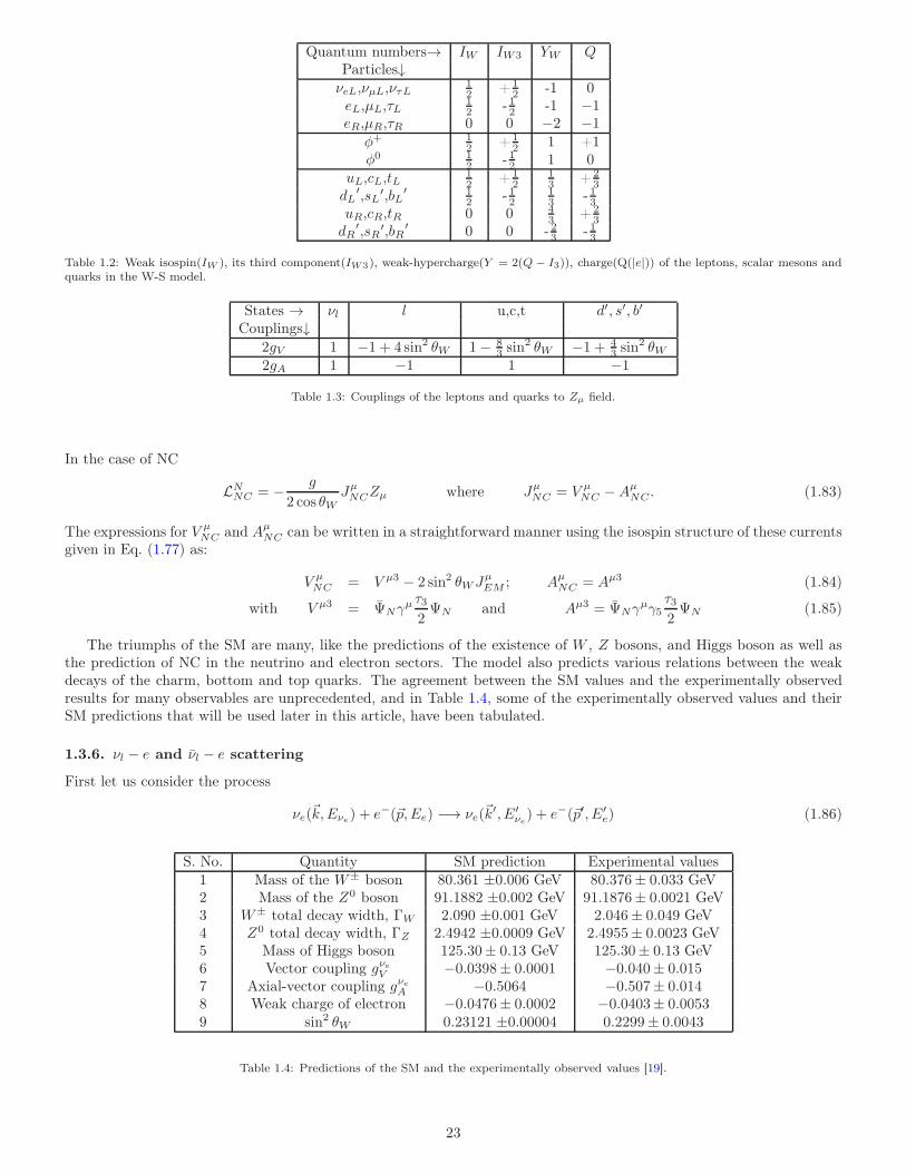
Quantum numbers→ IW IW3 YW QParticles↓νeL,νµL,ντL

12 + 1

2 -1 0eL,µL,τL

12 - 12 -1 −1

eR,µR,τR 0 0 −2 −1φ+ 1

2 + 12 1 +1

φ0 12 - 12 1 0

uL,cL,tL12 + 1

213 + 2

3dL

′,sL′,bL′ 1

2 - 1213 - 13

uR,cR,tR 0 0 43 + 2

3dR

′,sR′,bR′ 0 0 - 23 - 13

Table 1.2: Weak isospin(IW ), its third component(IW3), weak-hypercharge(Y = 2(Q − I3)), charge(Q(|e|)) of the leptons, scalar mesons andquarks in the W-S model.

States → νl l u,c,t d′, s′, b′

Couplings↓2gV 1 −1 + 4 sin2 θW 1− 8

3 sin2 θW −1 + 4

3 sin2 θW

2gA 1 −1 1 −1

Table 1.3: Couplings of the leptons and quarks to Zµ field.

In the case of NC

LNNC = − g

2 cos θWJµNCZµ where Jµ

NC = V µNC −A

µNC . (1.83)

The expressions for V µNC and Aµ

NC can be written in a straightforward manner using the isospin structure of these currentsgiven in Eq. (1.77) as:

V µNC = V µ3 − 2 sin2 θWJµ

EM ; AµNC = Aµ3 (1.84)

with V µ3 = ΨNγµ τ32ΨN and Aµ3 = ΨNγ

µγ5τ32ΨN (1.85)

The triumphs of the SM are many, like the predictions of the existence of W , Z bosons, and Higgs boson as well asthe prediction of NC in the neutrino and electron sectors. The model also predicts various relations between the weakdecays of the charm, bottom and top quarks. The agreement between the SM values and the experimentally observedresults for many observables are unprecedented, and in Table 1.4, some of the experimentally observed values and theirSM predictions that will be used later in this article, have been tabulated.

1.3.6. νl − e and νl − e scattering

First let us consider the process

νe(~k,Eνe) + e−(~p,Ee) −→ νe(~k′, E′

νe) + e−(~p′, E′e) (1.86)

S. No. Quantity SM prediction Experimental values1 Mass of the W± boson 80.361 ±0.006 GeV 80.376± 0.033 GeV2 Mass of the Z0 boson 91.1882 ±0.002 GeV 91.1876± 0.0021 GeV3 W± total decay width, ΓW 2.090 ±0.001 GeV 2.046± 0.049 GeV4 Z0 total decay width, ΓZ 2.4942 ±0.0009 GeV 2.4955± 0.0023 GeV5 Mass of Higgs boson 125.30± 0.13 GeV 125.30± 0.13 GeV6 Vector coupling gνeV −0.0398± 0.0001 −0.040± 0.0157 Axial-vector coupling gνeA −0.5064 −0.507± 0.0148 Weak charge of electron −0.0476± 0.0002 −0.0403± 0.00539 sin2 θW 0.23121 ±0.00004 0.2299± 0.0043

Table 1.4: Predictions of the SM and the experimentally observed values [19].

23

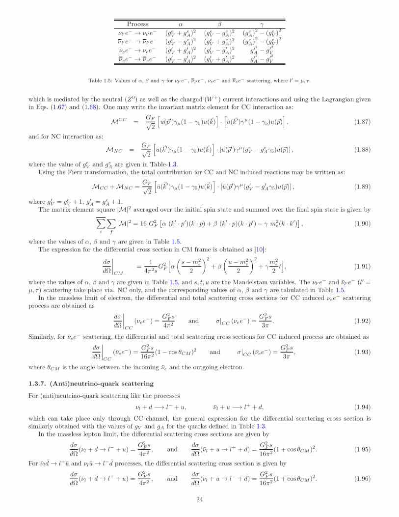
Process α β γ

νl′e− → νl′e

− (geV + geA)2 (geV − geA)2 (geA)

2 − (geV )2

νl′e− → νl′e

− (geV − geA)2 (geV + geA)2 (geA)

2 − (geV )2

νee− → νee

− (g′V + g′A)2 (g′V − g′A)2 g′

2

A − g′2

V

νee− → νee

− (g′V − g′A)2 (g′V + g′A)2 g′

2

A − g′2

V

Table 1.5: Values of α, β and γ for νl′e−, νl′e

−, νee− and νee− scattering, where l′ = µ, τ .

which is mediated by the neutral (Z0) as well as the charged (W+) current interactions and using the Lagrangian givenin Eqs. (1.67) and (1.68). One may write the invariant matrix element for CC interaction as:

MCC =GF√2

[

u(~p′)γµ(1− γ5)u(~k)]

·[

u(~k′)γµ(1− γ5)u(~p)]

, (1.87)

and for NC interaction as:

MNC =GF√2

[

u(~k′)γµ(1 − γ5)u(~k)]

· [u(~p′)γµ(geV − geAγ5)u(~p)] , (1.88)

where the value of geV and geA are given in Table-1.3.Using the Fierz transformation, the total contribution for CC and NC induced reactions may be written as:

MCC +MNC =GF√2

[

u(~k′)γµ(1− γ5)u(~k)]

· [u(~p′)γµ(g′V − g′Aγ5)u(~p)] , (1.89)

where g′V = geV + 1, g′A = geA + 1.The matrix element square |M|2 averaged over the initial spin state and summed over the final spin state is given by

∑

i

∑

f

|M|2 = 16 G2F

[

α (k′ · p′)(k · p) + β (k′ · p)(k · p′)− γ m2e(k · k′)

]

, (1.90)

where the values of α, β and γ are given in Table 1.5.The expression for the differential cross section in CM frame is obtained as [10]:

dσ

dΩ

∣

∣

∣

∣

CM

=1

4π2sG2

F

[

α

(

s−m2e

2

)2

+ β

(

u−m2e

2

)2

+ γm2

e

2t]

, (1.91)

where the values of α, β and γ are given in Table 1.5, and s, t, u are the Mandelstam variables. The νl′e− and νl′e

− (l′ =µ, τ) scattering take place via. NC only, and the corresponding values of α, β and γ are tabulated in Table 1.5.

In the massless limit of electron, the differential and total scattering cross sections for CC induced νee− scattering

process are obtained as

dσ

dΩ

∣

∣

∣

∣

CC

(νee−) =

G2F s

4π2and σ|CC (νee

−) =G2

F s

3π. (1.92)

Similarly, for νee− scattering, the differential and total scattering cross sections for CC induced process are obtained as

dσ

dΩ

∣

∣

∣

∣

CC

(νee−) =

G2F s

16π2(1− cos θCM )2 and σ|CC (νee

−) =G2

F s

3π, (1.93)

where θCM is the angle between the incoming νe and the outgoing electron.

1.3.7. (Anti)neutrino-quark scattering

For (anti)neutrino-quark scattering like the processes

νl + d −→ l− + u, νl + u −→ l+ + d, (1.94)

which can take place only through CC channel, the general expression for the differential scattering cross section issimilarly obtained with the values of gV and gA for the quarks defined in Table 1.3.

In the massless lepton limit, the differential scattering cross sections are given by

dσ

dΩ(νl + d→ l− + u) =

G2F s

4π2, and

dσ

dΩ(νl + u→ l+ + d) =

G2F s

16π2(1 + cos θCM )2. (1.95)

For νld→ l+u and νlu→ l−d processes, the differential scattering cross section is given by

dσ

dΩ(νl + d→ l+ + u) =

G2F s

4π2, and

dσ

dΩ(νl + u→ l− + d) =

G2F s

16π2(1 + cos θCM )2. (1.96)

24

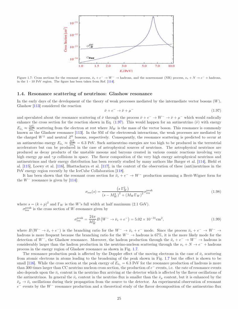
Figure 1.7: Cross sections for the resonant process, νe + e− → W− → hadrons, and the nonresonant (NR) process, νe +N → e− + hadrons,in the 1 - 10 PeV region. The figure has been taken from Ref. [114].

1.4. Resonance scattering of neutrinos: Glashow resonance

In the early days of the development of the theory of weak processes mediated by the intermediate vector bosons (W ),Glashow [113] considered the reaction

ν + e− → ν + µ− (1.97)

and speculated about the resonance scattering of ν through the process ν + e− → W− → ν + µ− which would radicallyenhance the cross section for the reaction shown in Eq. (1.97). This would happen for an antineutrino (ν) with energy

Eνe ≈M2

W

2mescattering from the electron at rest where MW is the mass of the vector boson. This resonance is commonly

known as the Glashow resonance [113]. In the SM of the electroweak interactions, the weak processes are mediated bythe charged W± and neutral Z0 bosons, respectively. Consequently, the resonance scattering is predicted to occur at

an antineutrino energy Eνe ≈M2

W

2me= 6.3 PeV. Such antineutrino energies are too high to be produced in the terrestrial

accelerators but can be produced in the case of astrophysical sources of neutrinos. The astrophysical neutrinos areproduced as decay products of the unstable mesons and baryons created in various cosmic reactions involving veryhigh energy pp and γp collisions in space. The flavor composition of the very high energy astrophysical neutrinos andantineutrinos and their energy distribution has been recently studied by many authors like Barger et al. [114], Biehl etal. [115], Loewy et al. [116], Bhattacharya et al. [117], in the context of the observation of these (anti)neutrinos in thePeV energy region recently by the IceCube Collaboration [118].

It has been shown that the resonant cross section for νe + e− → W− production assuming a Breit-Wigner form forthe W− resonance is given by [114]:

σres(s) =

(

s Γ2W

)

(s−M2W )

2+ (MWΓW )2

σpeakres (1.98)

where s = (k + p)2 and ΓW is the W ’s full width at half maximum (2.1 GeV).σpeak

res is the cross section of W -resonance given by

σpeakres =

24π

M2W

B(

W− → νe + e−)

= 5.02× 10−31cm2, (1.99)

where B (W− → νe + e−) is the branching ratio for the W− → νe + e− mode. Since the process νe + e− → W− →hadrons is more frequent because the branching ratio for the W− → hadrons is 67%, it is the more likely mode for thedetection of W−, the Glashow resonance. Moreover, the hadron production through the νe + e− → W− → hadrons isconsiderably larger than the hadron production in the neutrino-nucleon scattering through the νe + N → e− + hadronsprocess in the energy region of Glashow resonance as shown in Fig. 1.7.

The resonance production peak is affected by the Doppler effect of the moving electrons in the case of νe scatteringfrom atomic electrons in atoms leading to the broadening of the peak shown in Fig. 1.7 but the effect is shown to besmall [116]. While the cross section at the peak energy of Eνe = 6.3 PeV for the resonance production of hadrons is morethan 300 times larger than CC neutrino nucleon cross section, the production of e− events, i.e. the rate of resonance eventsalso depends upon the νe content in the neutrino flux arriving at the detector which is affected by the flavor oscillations ofthe antineutrinos. In general the νe content in the neutrino flux is smaller than the νµ content, but it is enhanced by theνµ → νe oscillations during their propagation from the source to the detector. An experimental observation of resonante− events by the W− resonance production and a theoretical study of the flavor decomposition of the antineutrino flux

25

generated in the various neutrino producing reactions from the high energy pp and γp reactions in space including theeffect of flavor oscillations of neutrinos, will provide important information about the source and production mechanismof very high energy neutrinos in the PeV energy region.

A recent report of the IceCube neutrino observatory [118] has claimed to observe one event of a cascade of high energyparticle shower with a visible energy of 6.05 ± 0.72 PeV detected from the Cherenkov radiation of the shower particles,which is claimed to be due to the Glashow resonance. After correcting the visible energy for shower particles which do notradiate, the neutrino energy is inferred to be 6.3 PeV consistent with the prediction of the SM. The IceCube Generation-2experiment [119] planned for future would improve the statistics and enable to measure the high energy antineutrino fluxwhich would give information about the different mechanism for producing high energy astrophysical neutrinos in thePeV region and enrich our knowledge of the neutrino astronomy.

2. Neutrino scattering from nucleons

Neutrino experiments are done in the wide range of energy starting from a few MeV to TeV region using solar, reactor,atmospheric, and accelerator (anti)neutrinos. The present goal of the experimenters is to measure with better precisionthe various neutrino oscillation parameters, like the mixing angles, the mass-squared-difference of the neutrino masseigenstates, CP violating phase δ in the lepton sector as well as to determine the mass hierarchy of the neutrino masseigenstates. These parameters are sensitive to the neutrinos of different energy range which are obtained from accelerator,atmospheric, reactor and solar neutrino and/or (anti)neutrinos sources as mentioned in Section-1.1.3 and summarizedin Table-1.1. Almost all the current generation (anti)neutrino experiments are using moderate to heavy nuclear targets.These experiments are measuring (anti)neutrino events which are convolution of energy dependent (anti)neutrino fluxand the energy dependent neutrino-nucleus cross section where NME play very important role. In the precision era ofneutrino physics, to achieve an accuracy of a few percent (2–3%) in the systematics, a good understanding of the neutrino-nucleon and neutrino-nucleus cross sections is highly desirable both experimentally as well as theoretically, which hasbeen highlighted by various review articles [120, 121, 122, 123]. Apart from being significant to the determination ofneutrino oscillation parameters, the neutrino-nucleon and neutrino-nucleus cross sections are important in their ownright as they provide information about the axial-vector response of the nucleons bound inside the nucleus, which isnot accessible via. photon or electron induced reactions, and recently it has been suggested [124] to perform neutrinoexperiments using hydrogen and deuterium targets. In this section, we focus on the neutrino-nucleon reactions and takeup the neutrino-nucleus reactions in Section 5.

The (anti)neutrino interaction with a nucleon target starts with the elastic and quasielastic (QE) scattering processes.With the increase in available neutrino energies, the inelastic (IE) reactions in which new particles like 1π, multiple pions,1η, 1K, Y π, and Y K (Y = Λ,Σ,Ξ), etc. are created as well as the deep inelastic scattering (DIS) become possible whichare diagrammatically shown in Fig. 2.1 and described below [10]:

• Elastic and quasielastic scattering: Neutrinos and antineutrinos of all flavors interact with a nucleon throughCC as well as NC interactions,

νℓ/νℓ +N −→ ℓ−/ℓ+ +N ′, (CC), (2.1)

and νℓ/νℓ +N −→ νℓ/νℓ +N (NC) (2.2)

in the ∆S = 0 sector, and

νℓ +N −→ ℓ+ + Y, (CC) (2.3)

in the ∆S = 1 sector; where N,N ′ = n, p and Y = Λ,Σ−,0.

It may be noticed that in the strangeness sector, single hyperon (like Λ,Σ−,0, etc.) produced in the final states, arepossible only in the antineutrino induced reactions while it is prohibited in neutrino channel due to the ∆S = ∆Qand FCNC rules.

• Inelastic scattering: The IE processes like the single and multiple mesons are produced in the CC and NCreactions subject to the absence of FCNC. A list of such reactions is given in Table-2.1.

• Deep inelastic scattering: The DIS processes induced by the CC and NC interactions are represented by thereactions

νℓ/νℓ +N −→ ℓ−/ℓ+ +X, νℓ/νℓ +N −→ νℓ/νℓ +X. (2.4)

where X is jet of hadrons in the final state.

26

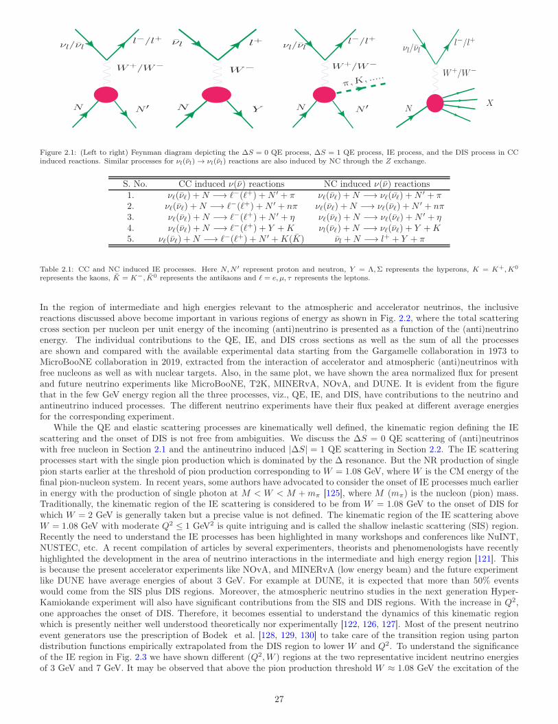
νl/νll−/l+

W+/W−

N N ′

νl l+

W−

N Y

π,K, .....

N N ′

νl/νll−/l+

W+/W−

νl/νll−/l+

W+/W−

NX

Figure 2.1: (Left to right) Feynman diagram depicting the ∆S = 0 QE process, ∆S = 1 QE process, IE process, and the DIS process in CCinduced reactions. Similar processes for νl(νl) → νl(νl) reactions are also induced by NC through the Z exchange.

S. No. CC induced ν(ν) reactions NC induced ν(ν) reactions1. νℓ(νℓ) +N −→ ℓ−(ℓ+) +N ′ + π νℓ(νℓ) +N −→ νℓ(νℓ) +N ′ + π2. νℓ(νℓ) +N −→ ℓ−(ℓ+) +N ′ + nπ νℓ(νℓ) +N −→ νℓ(νℓ) +N ′ + nπ3. νℓ(νℓ) +N −→ ℓ−(ℓ+) +N ′ + η νℓ(νℓ) +N −→ νℓ(νℓ) +N ′ + η4. νℓ(νℓ) +N −→ ℓ−(ℓ+) + Y +K νl(νℓ) +N −→ νℓ(νℓ) + Y +K5. νℓ(νℓ) +N −→ ℓ−(ℓ+) +N ′ +K(K) νl +N −→ l+ + Y + π

Table 2.1: CC and NC induced IE processes. Here N,N ′ represent proton and neutron, Y = Λ,Σ represents the hyperons, K = K+,K0

represents the kaons, K = K−, K0 represents the antikaons and ℓ = e, µ, τ represents the leptons.

In the region of intermediate and high energies relevant to the atmospheric and accelerator neutrinos, the inclusivereactions discussed above become important in various regions of energy as shown in Fig. 2.2, where the total scatteringcross section per nucleon per unit energy of the incoming (anti)neutrino is presented as a function of the (anti)neutrinoenergy. The individual contributions to the QE, IE, and DIS cross sections as well as the sum of all the processesare shown and compared with the available experimental data starting from the Gargamelle collaboration in 1973 toMicroBooNE collaboration in 2019, extracted from the interaction of accelerator and atmospheric (anti)neutrinos withfree nucleons as well as with nuclear targets. Also, in the same plot, we have shown the area normalized flux for presentand future neutrino experiments like MicroBooNE, T2K, MINERvA, NOvA, and DUNE. It is evident from the figurethat in the few GeV energy region all the three processes, viz., QE, IE, and DIS, have contributions to the neutrino andantineutrino induced processes. The different neutrino experiments have their flux peaked at different average energiesfor the corresponding experiment.

While the QE and elastic scattering processes are kinematically well defined, the kinematic region defining the IEscattering and the onset of DIS is not free from ambiguities. We discuss the ∆S = 0 QE scattering of (anti)neutrinoswith free nucleon in Section 2.1 and the antineutrino induced |∆S| = 1 QE scattering in Section 2.2. The IE scatteringprocesses start with the single pion production which is dominated by the ∆ resonance. But the NR production of singlepion starts earlier at the threshold of pion production corresponding to W = 1.08 GeV, where W is the CM energy of thefinal pion-nucleon system. In recent years, some authors have advocated to consider the onset of IE processes much earlierin energy with the production of single photon at M < W < M +mπ [125], where M (mπ) is the nucleon (pion) mass.Traditionally, the kinematic region of the IE scattering is considered to be from W = 1.08 GeV to the onset of DIS forwhich W = 2 GeV is generally taken but a precise value is not defined. The kinematic region of the IE scattering aboveW = 1.08 GeV with moderate Q2 ≤ 1 GeV2 is quite intriguing and is called the shallow inelastic scattering (SIS) region.Recently the need to understand the IE processes has been highlighted in many workshops and conferences like NuINT,NUSTEC, etc. A recent compilation of articles by several experimenters, theorists and phenomenologists have recentlyhighlighted the development in the area of neutrino interactions in the intermediate and high energy region [121]. Thisis because the present accelerator experiments like NOvA, and MINERvA (low energy beam) and the future experimentlike DUNE have average energies of about 3 GeV. For example at DUNE, it is expected that more than 50% eventswould come from the SIS plus DIS regions. Moreover, the atmospheric neutrino studies in the next generation Hyper-Kamiokande experiment will also have significant contributions from the SIS and DIS regions. With the increase in Q2,one approaches the onset of DIS. Therefore, it becomes essential to understand the dynamics of this kinematic regionwhich is presently neither well understood theoretically nor experimentally [122, 126, 127]. Most of the present neutrinoevent generators use the prescription of Bodek et al. [128, 129, 130] to take care of the transition region using partondistribution functions empirically extrapolated from the DIS region to lower W and Q2. To understand the significanceof the IE region in Fig. 2.3 we have shown different (Q2,W ) regions at the two representative incident neutrino energiesof 3 GeV and 7 GeV. It may be observed that above the pion production threshold W ≈ 1.08 GeV the excitation of the

27

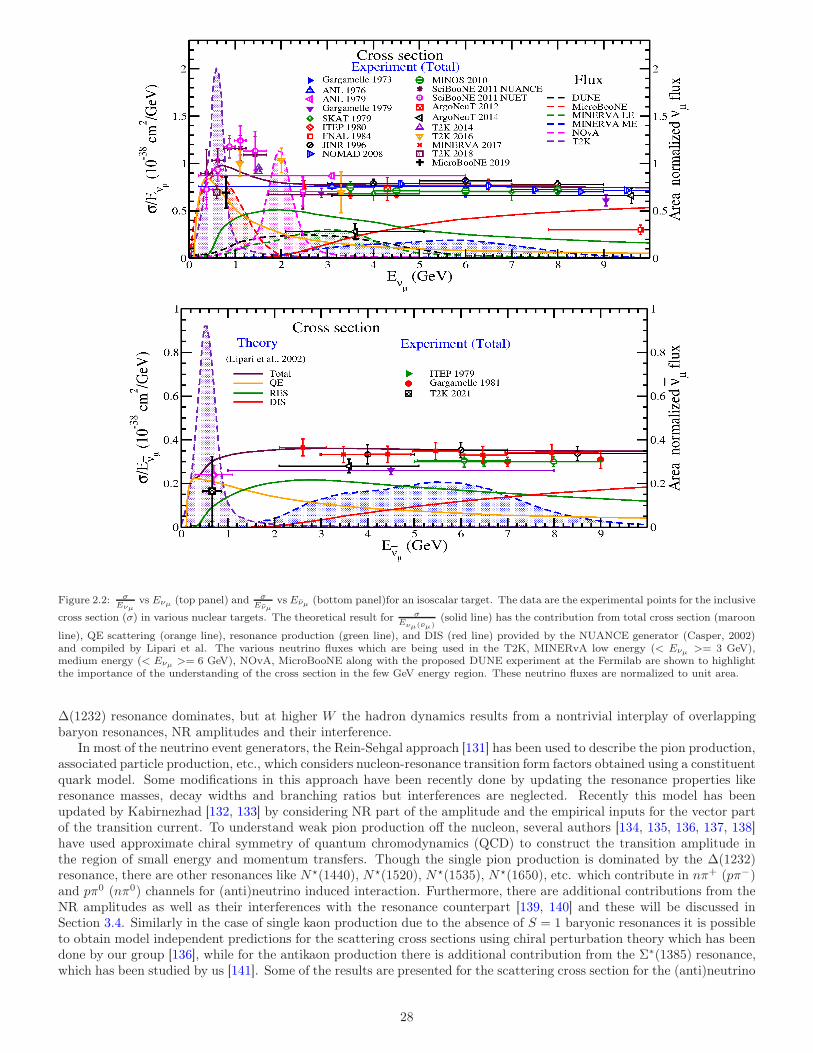
Figure 2.2: σEνµ

vs Eνµ (top panel) and σEνµ

vs Eνµ (bottom panel)for an isoscalar target. The data are the experimental points for the inclusive

cross section (σ) in various nuclear targets. The theoretical result for σEνµ(νµ)

(solid line) has the contribution from total cross section (maroon

line), QE scattering (orange line), resonance production (green line), and DIS (red line) provided by the NUANCE generator (Casper, 2002)and compiled by Lipari et al. The various neutrino fluxes which are being used in the T2K, MINERvA low energy (< Eνµ >= 3 GeV),medium energy (< Eνµ >= 6 GeV), NOvA, MicroBooNE along with the proposed DUNE experiment at the Fermilab are shown to highlightthe importance of the understanding of the cross section in the few GeV energy region. These neutrino fluxes are normalized to unit area.

∆(1232) resonance dominates, but at higher W the hadron dynamics results from a nontrivial interplay of overlappingbaryon resonances, NR amplitudes and their interference.

In most of the neutrino event generators, the Rein-Sehgal approach [131] has been used to describe the pion production,associated particle production, etc., which considers nucleon-resonance transition form factors obtained using a constituentquark model. Some modifications in this approach have been recently done by updating the resonance properties likeresonance masses, decay widths and branching ratios but interferences are neglected. Recently this model has beenupdated by Kabirnezhad [132, 133] by considering NR part of the amplitude and the empirical inputs for the vector partof the transition current. To understand weak pion production off the nucleon, several authors [134, 135, 136, 137, 138]have used approximate chiral symmetry of quantum chromodynamics (QCD) to construct the transition amplitude inthe region of small energy and momentum transfers. Though the single pion production is dominated by the ∆(1232)resonance, there are other resonances like N⋆(1440), N⋆(1520), N⋆(1535), N⋆(1650), etc. which contribute in nπ+ (pπ−)and pπ0 (nπ0) channels for (anti)neutrino induced interaction. Furthermore, there are additional contributions from theNR amplitudes as well as their interferences with the resonance counterpart [139, 140] and these will be discussed inSection 3.4. Similarly in the case of single kaon production due to the absence of S = 1 baryonic resonances it is possibleto obtain model independent predictions for the scattering cross sections using chiral perturbation theory which has beendone by our group [136], while for the antikaon production there is additional contribution from the Σ∗(1385) resonance,which has been studied by us [141]. Some of the results are presented for the scattering cross section for the (anti)neutrino

28

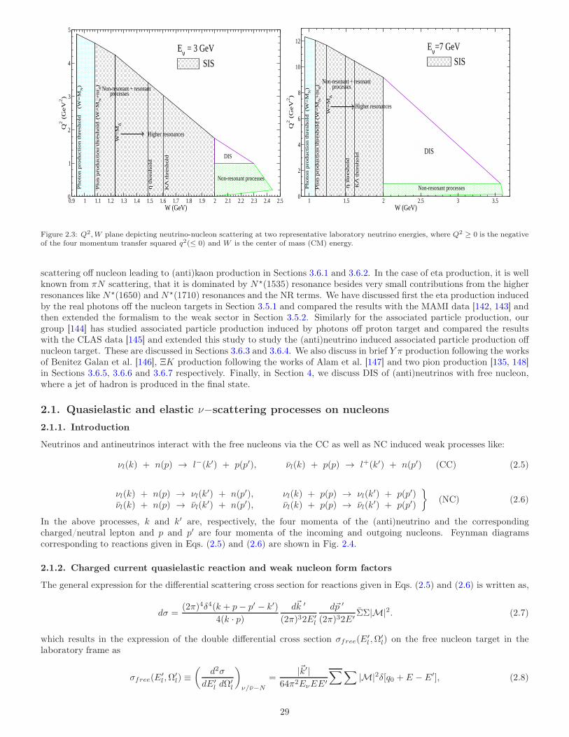
0.9 1 1.1 1.2 1.3 1.4 1.5 1.6 1.7 1.8 1.9 2 2.1 2.2 2.3 2.4 2.5W (GeV)

0

1

2

3

4

5

Q2 (

GeV

2)

Eν = 3 GeV

DISη

thre

shold

Higher resonances

Non-resonant + resonantprocesses

Pio

n p

roducti

on t

hre

shold

Photo

n p

roducti

on t

hre

shold

(W

=M

N)

(W=

MN

+m

π)

W=

M∆

SIS

Non-resonant processes

KΛ

thre

shold

1 1.5 2 2.5 3 3.5W (GeV)

0

2

4

6

8

10

12

Q2 (

GeV

2)

Eν=7 GeV

DIS

η t

hre

shold

Higher resonances

Non-resonant + resonant

Photo

n p

roducti

on t

hre

shold

KΛ

thre

shold

(W=

MN

)

Pio

n p

roducti

on t

hre

shold

(W

=M

N+

mπ)

W=

M∆

Non-resonant processes

SIS

processes

Figure 2.3: Q2,W plane depicting neutrino-nucleon scattering at two representative laboratory neutrino energies, where Q2 ≥ 0 is the negativeof the four momentum transfer squared q2(≤ 0) and W is the center of mass (CM) energy.

scattering off nucleon leading to (anti)kaon production in Sections 3.6.1 and 3.6.2. In the case of eta production, it is wellknown from πN scattering, that it is dominated by N⋆(1535) resonance besides very small contributions from the higherresonances like N⋆(1650) and N⋆(1710) resonances and the NR terms. We have discussed first the eta production inducedby the real photons off the nucleon targets in Section 3.5.1 and compared the results with the MAMI data [142, 143] andthen extended the formalism to the weak sector in Section 3.5.2. Similarly for the associated particle production, ourgroup [144] has studied associated particle production induced by photons off proton target and compared the resultswith the CLAS data [145] and extended this study to study the (anti)neutrino induced associated particle production offnucleon target. These are discussed in Sections 3.6.3 and 3.6.4. We also discuss in brief Y π production following the worksof Benitez Galan et al. [146], ΞK production following the works of Alam et al. [147] and two pion production [135, 148]in Sections 3.6.5, 3.6.6 and 3.6.7 respectively. Finally, in Section 4, we discuss DIS of (anti)neutrinos with free nucleon,where a jet of hadron is produced in the final state.

2.1. Quasielastic and elastic ν−scattering processes on nucleons

2.1.1. Introduction

Neutrinos and antineutrinos interact with the free nucleons via the CC as well as NC induced weak processes like:

νl(k) + n(p) → l−(k′) + p(p′), νl(k) + p(p) → l+(k′) + n(p′) (CC) (2.5)

νl(k) + n(p) → νl(k′) + n(p′), νl(k) + p(p) → νl(k

′) + p(p′)νl(k) + n(p) → νl(k

′) + n(p′), νl(k) + p(p) → νl(k′) + p(p′)

(NC) (2.6)

In the above processes, k and k′ are, respectively, the four momenta of the (anti)neutrino and the correspondingcharged/neutral lepton and p and p′ are four momenta of the incoming and outgoing nucleons. Feynman diagramscorresponding to reactions given in Eqs. (2.5) and (2.6) are shown in Fig. 2.4.

2.1.2. Charged current quasielastic reaction and weak nucleon form factors

The general expression for the differential scattering cross section for reactions given in Eqs. (2.5) and (2.6) is written as,

dσ =(2π)4δ4(k + p− p′ − k′)

4(k · p)d~k ′

(2π)32E′l

d~p ′

(2π)32E′ ΣΣ|M|2. (2.7)

which results in the expression of the double differential cross section σfree(E′l ,Ω

′l) on the free nucleon target in the

laboratory frame as

σfree(E′l ,Ω

′l) ≡

(

d2σ

dE′l dΩ

′l

)

ν/ν−N

=|~k′|

64π2EνEE′

∑∑

|M|2δ[q0 + E − E′], (2.8)

29

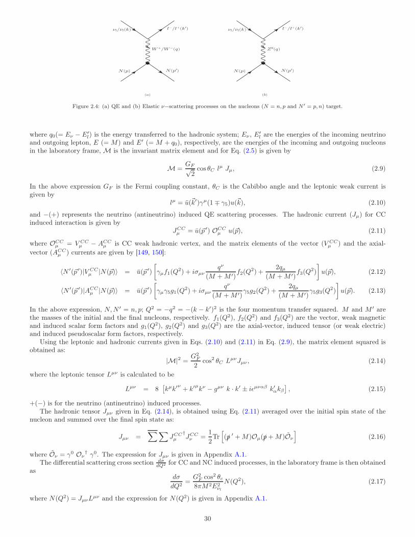
νl/νl(k) l−/l+(k′)

N(p) N(p′)

W+/W−(q)

νl/νl(k) l−/l+(k′)

N(p) N(p′)

Z0(q)

(a) (b)

Figure 2.4: (a) QE and (b) Elastic ν−scattering processes on the nucleons (N = n, p and N ′ = p, n) target.

where q0(= Eν − E′l) is the energy transferred to the hadronic system; Eν , E′

l are the energies of the incoming neutrinoand outgoing lepton, E (= M) and E′ (= M + q0), respectively, are the energies of the incoming and outgoing nucleonsin the laboratory frame,M is the invariant matrix element and for Eq. (2.5) is given by

M =GF√2cos θC lµ Jµ, (2.9)

In the above expression GF is the Fermi coupling constant, θC is the Cabibbo angle and the leptonic weak current isgiven by

lµ = u(~k′)γµ(1∓ γ5)u(~k), (2.10)

and −(+) represents the neutrino (antineutrino) induced QE scattering processes. The hadronic current (Jµ) for CCinduced interaction is given by

JCCµ = u(~p ′) OCC

µ u(~p), (2.11)

where OCCµ = V CC

µ − ACCµ is CC weak hadronic vertex, and the matrix elements of the vector (V CC

µ ) and the axial-

vector (ACCµ ) currents are given by [149, 150]:

〈N ′(~p ′)|V CCµ |N(~p)〉 = u(~p ′)

[

γµf1(Q2) + iσµν

qν

(M +M ′)f2(Q

2) +2qµ

(M +M ′)f3(Q

2)

]

u(~p), (2.12)

〈N ′(~p ′)|ACCµ |N(~p)〉 = u(~p ′)

[

γµγ5g1(Q2) + iσµν

qν

(M +M ′)γ5g2(Q

2) +2qµ

(M +M ′)γ5g3(Q

2)

]

u(~p). (2.13)

In the above expression, N,N ′ = n, p; Q2 = −q2 = −(k − k′)2 is the four momentum transfer squared. M and M ′ arethe masses of the initial and the final nucleons, respectively. f1(Q

2), f2(Q2) and f3(Q

2) are the vector, weak magneticand induced scalar form factors and g1(Q

2), g2(Q2) and g3(Q

2) are the axial-vector, induced tensor (or weak electric)and induced pseudoscalar form factors, respectively.

Using the leptonic and hadronic currents given in Eqs. (2.10) and (2.11) in Eq. (2.9), the matrix element squared isobtained as:

|M|2 =G2

F

2cos2 θC LµνJµν , (2.14)

where the leptonic tensor Lµν is calculated to be

Lµν = 8[

kµk′ν+ k′

µkν − gµν k · k′ ± iǫµναβ k′αkβ

]

, (2.15)

+(−) is for the neutrino (antineutrino) induced processes.The hadronic tensor Jµν given in Eq. (2.14), is obtained using Eq. (2.11) averaged over the initial spin state of the

nucleon and summed over the final spin state as:

Jµν =∑∑

JCCµ

†JCCν =

1

2Tr[

(/p′ +M)Oµ(/p+M)Oν

]

(2.16)

where Oν = γ0 Oν† γ0. The expression for Jµν is given in Appendix A.1.

The differential scattering cross section dσdQ2 for CC and NC induced processes, in the laboratory frame is then obtained

asdσ

dQ2=G2

F cos2 θc8πM2E2

νl

N(Q2), (2.17)

where N(Q2) = JµνLµν and the expression for N(Q2) is given in Appendix A.1.

30

2.1.3. Neutral current elastic reactions and weak nucleon form factors

We define the hadronic current for the weak NC induced processes on the proton and the neutron targets, given inEq. (2.6), in terms of NC form factors fp,n

i (Q2) and gp,ni (Q2)(i = 1, 2, 3) for the protons and neutrons, respectively, as

JNCµ |i = u(~p ′)ONC

µ u(~p) = u(~p ′)

[

γµfi1(Q

2) +iσµνq

ν f i2(Q

2)

2M+qµMγ5f

i3(Q

2)

+ γµγ5gi1(Q

2) +(pµ + p′µ)

Mγ5g

i2(Q

2) +qµγ5g

i3(Q

2)

M

]

u(~p), (2.18)

with i = p, n. Here the nomenclature of the form factors is the same as in the case of CC QE process (Eqs. (2.12) and(2.13)) and the parameterization for fi(Q

2) and gi(Q2) are given in Section 2.1.5.

2.1.4. Symmetry properties of the weak hadronic current

The weak hadronic current Jµ has the vector Vµ and the axial-vector Aµ terms constructed using the bilinear covariantsassociated with the nucleon fields as well as the four momenta of the incoming and outgoing nucleons. These bilinearcovariants have certain definite properties under discrete transformation like C, P and T as well as the internal symmetrieslike the isospin and unitary symmetry [10, 150]. These symmetry properties are exploited in writing the matrix elementsof these currents between the initial and final states of spin 0, 1

2 , and 32 particles. We discuss below these symmetry

properties and their role in writing the general structure of the matrix elements.

(i) Isospin properties of the weak hadronic current

The weak hadronic currents between the neutron and proton states involve a change of charge ∆Q = ±1 in the caseof n→ p and p→ n transitions. Since Q = I3+

B2 for the nonstrange baryons, therefore ∆Q = ±1 implies ∆I3 = ±1

using baryon number conservation. Since protons and neutrons are assigned to a doublet, therefore, they can bewritten as a two component isospinor under the group of isospin transformation, i.e.

u =

(

upun

)

. (2.19)

The isospin group of transformations is generated by the three 2 × 2 Pauli matrices τi (i = 1 − 3), which alongwith the vector currents constitute the isovector part of the hadronic current. By defining the isospin raising andlowering operators τ± = τ1±iτ2

2 , we can write

upVCCµ un = uV CC

µ τ+u = uV CC+µ u, unV

CCµ up = uV CC

µ τ−u = uV CC−µ u. (2.20)

It may be observed from the above relations that the charged weak vector currents are purely isovector in nature.

Similarly, for the electromagnetic vector current, the hadronic current is given by

Jemµ(p,n)(p, p

′) = u(~p ′p,n)V

emµ u(~pp,n), (2.21)

with

V emµ (p, n) =

[

γµFp,n1 (Q2) + iσµν

qν

(2M)F p,n2 (Q2)

]

, (2.22)

where q = p′ − p with Q2 = −q2. F p,n1 (Q2) and F p,n

2 (Q2) are, respectively, the Dirac and Pauli form factors ofthe nucleon. In terms of the Pauli matrices, the hadronic currents for the electromagnetic induced interactions arewritten as

upVemµ up = uV em

µ

I+ τ32

u, unVemµ un = uV em

µ

I− τ32

u (2.23)

implying the isoscalar and isovector current matrix elements as

u 1V emµ u = upV

emµ up + unV

emµ un, uτ3V

emµ u = upV

emµ up − unV em

µ un. (2.24)

If we parameterize the matrix element of the isoscalar (with form factors FS1,2(Q

2)) and isovector (with form factors

FV1,2(Q

2)) components as

u 1V emµ u = u

[

FS1 (Q2)γµ + iFS

2 (Q2)σµνq

ν

2M

]

u, uτ3Vemµ u = u

[

FV1 (q2)γµ + i

σµνqν

2MFV2 (q2)

]

τ3u, (2.25)

31

and the electromagnetic matrix element of protons and neutrons given in Eq. (2.21) with Oemµ given in Eq. (2.22),

then we can write:

FS1,2(Q

2) = F p1,2(Q

2) + Fn1,2(Q

2), FV1,2(Q

2) = F p1,2(Q

2)− Fn1,2(Q

2). (2.26)

The above expression shows that the electromagnetic current transforms as the sum of the isoscalar and isovectorcurrents.

(ii) T invariance

Time reversal invariance holds ifM′ =M∗, (2.27)

whereM′ represents the time reversed matrix element andM∗ represents the Hermitian conjugate of the unreversedmatrix element. Under time-reversal invariance (T invariance), the initial and final state particles are interchangedas well as their spin and angular momenta are reversed.

Taking all the bilinear covariants used with the form factors in the vector and the axial-vector currents individually,we obtain the transformation of the vector and axial-vector form factors under T invariance as [10]:

upunT−−−→ unup, upγ5un

T−−−→ unγ5up,

upγµun

T−−−→ unγµup, upγµγ5un

T−−−→ unγµγ5up,

upσµνun

T−−−→ −unσµνup, upσµνγ5un

T−−−→ unσµνγ5up.

The hadronic current Jµ is defined in Eq. (2.11) with Vµ and Aµ defined in Eqs. (2.12) and (2.13), respectively. Thetime reversed current J ′

µ is obtained as [10]:

J ′µ = un

[

f1(Q2)γµ + iσµν

qν

M +M ′ f2(Q2) +

2qµM +M ′ f3(Q

2)

− g1(Q2)γµγ5 − iσµν

qν

M +M ′ γ5g2(Q2)− 2qµ

M +M ′ γ5g3(Q2)

]

up. (2.28)

Hermitian conjugate of Eq. (2.11) is written as

J∗µ = up

[

f∗1 (Q

2)γµ + iσµνqν

2Mf∗2 (Q

2) +qµMf∗3 (Q

2)− g∗1(Q2)γµγ5

− iσµνqν

2Mγ5g

∗2(Q

2)− qµMγ5g

∗3(Q

2)

]

un. (2.29)

Comparing Eqs. (2.28) and (2.29), we find that fi(Q2) = f∗

i (Q2) and gi(Q

2) = g∗i (Q2) which implies that if time

reversal invariance holds, the form factors must be real.

(iii) Conserved vector current hypothesis

The hypothesis of the conserved vector current (CVC) was proposed by Gershtein and Zeldovich [151] and Feynmanand Gell-Mann [12]. They made an important observation in the study of the nuclear β decays in Fermi transitiondriven by the vector currents, with no change in parity. They observed that the strength of the weak vectorcoupling (weak charge) for the muon and neutron decays are the same, just like in the case of the electromagneticinteractions where the strength of the electromagnetic coupling i.e. e, remains the same for the electrons and protons.Since the equality of the charge coupling, also known as the universality of the electromagnetic interactions followsfrom the conservation of the electromagnetic current, therefore, it was suggested that the weak vector current isalso conserved i.e. ∂µV

µ(x) = 0, which leads to the equality of the weak coupling for the leptons and hadrons.

In fact, they proposed a stronger hypothesis of the isotriplet of the vector currents which goes beyond the hypothesisof CVC and predicts the form factors f1,2(Q

2) describing the matrix elements of the weak vector current in termsof the electromagnetic form factors of hadrons. According to the isotriplet hypothesis, the weak vector currentsV +µ , V −

µ and the isovector part of the electromagnetic current V emµ are assumed to form an isotriplet under the

isospin symmetry such that f1 and f2 are given in terms of the isovector electromagnetic form factors i.e.

f1(Q2) = FV

1 (Q2) = F p1 (Q

2)− Fn1 (Q

2), f2(Q2) = FV

2 (Q2) = F p2 (Q

2)− Fn2 (Q

2). (2.30)

The CVC hypothesis, i.e. ∂µVµ(x) = 0 implies f3(Q

2) = 0. It should be noted that while the isotriplet currenthypothesis implies CVC due to the isospin symmetry, the vice versa is not true. In the literature, the term CVC ismostly used meaning both the isotriplet hypothesis of weak vector currents V +

µ and V −µ and the CVC hypothesis.

32

(iv) Partial conservation of axial-vector current

In contrast to the vector current which is conserved, the axial-vector current is not conserved. To see this explicitly,consider the matrix element of the axial-vector current between one pion state and vacuum which enters in the πl2decay of pion i.e. 〈0|Aµ(x) |π−〉 = ifπq

µe−iq·x, where q is the four momentum of the pion. Taking its divergenceleads to

< 0|∂µAµ(x)|π−(q) > = (−i)ifπqµqµe−iq.x = fπm2πe

−iq.x, (2.31)

as q2 = m2π. If the axial-vector current Aµ is divergenceless then either mπ = 0 or fπ = 0, implying the pion to be

massless or it does not decay. Since mπ 6= 0, conservation of axial-vector current implies fπ = 0, which is also nottrue. Therefore, the axial-vector current is not conserved. However, since the pion is the lightest hadron, we canwork in the limit of mπ → 0, and say that the axial-vector current is conserved in the limit

limmπ−→0

∂µAµ(x) = 0, (2.32)

which is termed as the partial conservation of axial-vector current (PCAC). The hypothesis of PCAC has beenvery useful in calculating many processes in the weak interaction physics and deriving relations between variousprocesses in the limit of mπ → 0. However, the real predictive power of PCAC lies in making further assumptionsabout the divergence of the axial-vector field ∂µA

µ(x) and identifying with the pion field φπ(x) that establishes aconnection between the weak and strong interaction physics and assuming that the transition amplitudes derived inthe mπ → 0 limit can be smoothly extrapolated to the physical mass of the pion. The success of PCAC in variousapplications of calculating the physical processes is based on the following assumptions:

(i) The divergence of the axial-vector field is a pseudoscalar field and the pion is also described by a pseudoscalarfield. If it is assumed that both are related i.e. then the physical pion field is described by the divergenceof the axial-vector current, i.e. ∂µA

µ(x) ∝ φπ(x), such that ∂µAµ(x) = eπφπ(x). This assumption makes it

possible to relate the weak interaction processes induced by Aµ to the pion physics in the strong interactionprocesses through the matrix element of its derivative i.e. ∂µA

µ.(ii) Taking the limit mπ → 0 (corresponding to the conserved axial-vector current) in the processes involving

pions and nucleons, makes it easier to evaluate the transition amplitude in many weak processes. If furtherassumption is made that these amplitudes vary smoothly with q2 and do not change much over the range of q2

involved in the processes, then the amplitudes evaluated at q2 = 0 can be extrapolated to the physical limit ofq2 = m2

π, i.e. f(0)→ f(m2π), where f(q2) is the pion form factor. This is called the soft pion limit widely used

in the weak interaction physics. However, there remains an ambiguity whether to take the limit as m2π → 0 or

mπ → 0 [152, 153]. For more discussion see Ref. [10].

(v) G-parity and second class currents

G-parity is a multiplicative quantum number, first used to classify the multipion states in pp and πp collisions [154,155, 156, 157] and later used by Weinberg [158] to classify the weak hadronic currents. It is defined as the productof C, the charge conjugation operation and a rotation by 1800 about the Y-axis in the isospin space i.e.

G = CeiπIY . (2.33)

Since strong interactions are invariant under C and isospin, they are also invariant under G-parity. The G-parityis a very useful concept in the study of pion production in NN collisions. Since the weak currents involve bilinearcovariants formed out of the nucleon fields ψ(p′) and ψ(p), their transformations can be well defined under G-parity. The weak vector and axial-vector currents between a neutron and a proton are defined in Eqs. (2.12) and(2.13). Since the currents belong to the triplet representation of the isospin, therefore, all the terms have similartransformation properties under the rotation eiπIY . It is their transformation properties under C-parity whichdefines their relative transformation properties under G-parity. Under C-parity, the bilinear terms in Eqs. (2.12)and (2.13) transforms as:

upunC−−→ −unup (assumed with f3) (2.34)

upγ5unC−−→ −upγ5un (assumed with g3) (2.35)

upγµγ5unC−−→ −upγµγ5up (assumed with g1) (2.36)

while

upγµun

C−−→ unγµup (assumed with f1) (2.37)

upσµνun

C−−→ unσµνup (assumed with f2) (2.38)

upσµνγ5un

C−−→ unσµνγ5up (assumed with g2) (2.39)

33

What is observed from Eqs. (2.34)–(2.39) is that the bilinear terms associated with f2 transforms the same way asf1 does, while f3 transforms in opposite way. Similarly, g3 transforms the same way as g1 does while g2 transformsin a different way. It was Weinberg [158] who first used the G-parity to classify the weak currents. He called thecurrents associated with f1, f2, g1 and g3 which are invariant under G-parity as the first class currents, and thecurrents associated with f3 and g2 which violate G-parity as the second class currents (SCC). Consequently, if Ginvariance is valid in the weak interactions then the currents with form factors f1(Q

2), f2(Q2), g1(Q

2) and g3(Q2)

should exist and f3(Q2) = g2(Q

2) = 0. It should be noted that f3(Q2) = 0 is also predicted as a consequence of

CVC hypothesis.

2.1.5. Parameterization of the weak form factors

(i) Vector form factorsIn the case of CC interactions, the hadronic current contains two isovector form factors f1,2(Q

2) of the nucleons,which can be related to the isovector combination of the Dirac (F p

1,2(Q2)) and Pauli (Fn

1,2(Q2)) form factors of the

proton and the neutron using the relation

f1,2(Q2) = F p

1,2(Q2)− Fn

1,2(Q2). (2.40)

The Dirac (F1(Q2)) and Pauli (F2(Q

2)) form factors are, in turn, expressed in terms of the experimentally determinedSachs’ electric (Gp,n

E (Q2)) and magnetic (Gp,nM (Q2)) form factors of the nucleon as:

F p,n1 (Q2) =

(

1 +Q2

4M2

)−1 [

Gp,nE (Q2) +

Q2

4M2Gp,n

M (Q2)

]

, (2.41)

F p,n2 (Q2) =

(

1 +Q2

4M2

)−1[

Gp,nM (Q2)−Gp,n

E (Q2)]

. (2.42)

Initially, it was observed from the experimental data of the electromagnetic scattering that the Sachs’ form factorsmay have a dipole form. However, with the development of electron beam accelerator experiments, it was observedthat the Sachs’ form form factors deviate from the dipole form. Galster et al. [159] parameterized the deviatedSachs’ form factors as

GpE(Q

2) = GD(Q2) GpM (Q2) = (1 + µp)GD(Q2)

GnM (Q2) = µnGD(Q2) Gn

E(Q2) = −( Q

2

4M2)µnGD(Q2)ξn

ξn =1

(

1− λn q2

4M2

) , GD(Q2) =1

(

1 + Q2

M2V

)2 ,

with µp = 1.7927µN , µn = −1.913µN , MV = 0.84 GeV and λn = 5.6.

Recently for Gp,nE (Q2) and Gp,n

M (Q2), various parameterizations are available in the literature like BBBA05 param-eterized by Bradford et al. [160], BBA03 parameterized by Budd et al. [161], Alberico et al. [162], Bosted [163],modified Galster parameterization given by Platchkov et al. [164], Kelly [165], and modified Kelly parameterizationgiven by Punjabi et al. [166]. We have used, in our numerical calculations, the parameterization given by Bradfordet al. [160].

The vector form factors for NC induced processes are obtained as

fp1,2(Q

2) =

(

1

2− 2 sin2 θW

)

F p1,2(Q

2)− 1

2Fn1,2(Q

2)− 1

2F s1,2(Q

2), (2.43)

fn1,2(Q

2) =

(

1

2− 2 sin2 θW

)

Fn1,2(Q

2)− 1

2F p1,2(Q

2)− 1

2F s1,2(Q

2), (2.44)

where θW is the Weinberg angle, and F s1 (Q

2) and F s2 (Q

2) are the strangeness vector form factors, which are discussedlater in this section.

(ii) Axial vector form factorThe isovector axial-vector form factor is parameterized as

g1(Q2) = gA(0)

(

1 +Q2

M2A

)−2

, (2.45)

34

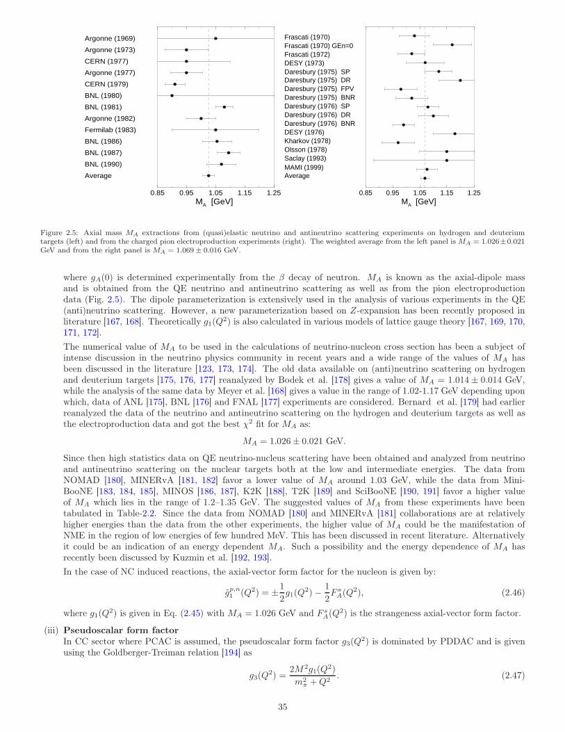
0.85 0.95 1.05 1.15 1.25MA [GeV]

Average

Argonne (1969)

CERN (1977)

Argonne (1977)

CERN (1979)

BNL (1980)

BNL (1981)

Argonne (1982)

Fermilab (1983)

BNL (1986)

BNL (1987)

BNL (1990)

Argonne (1973)

0.85 0.95 1.05 1.15 1.25MA [GeV]

Frascati (1970)Frascati (1970) GEn=0Frascati (1972)DESY (1973)Daresbury (1975) SPDaresbury (1975) DRDaresbury (1975) FPVDaresbury (1975) BNR

AverageMAMI (1999)Saclay (1993)Olsson (1978)Kharkov (1978)DESY (1976)

Daresbury (1976) SP

Daresbury (1976) BNRDaresbury (1976) DR

Figure 2.5: Axial mass MA extractions from (quasi)elastic neutrino and antineutrino scattering experiments on hydrogen and deuteriumtargets (left) and from the charged pion electroproduction experiments (right). The weighted average from the left panel is MA = 1.026±0.021GeV and from the right panel is MA = 1.069± 0.016 GeV.

where gA(0) is determined experimentally from the β decay of neutron. MA is known as the axial-dipole massand is obtained from the QE neutrino and antineutrino scattering as well as from the pion electroproductiondata (Fig. 2.5). The dipole parameterization is extensively used in the analysis of various experiments in the QE(anti)neutrino scattering. However, a new parameterization based on Z-expansion has been recently proposed inliterature [167, 168]. Theoretically g1(Q

2) is also calculated in various models of lattice gauge theory [167, 169, 170,171, 172].

The numerical value of MA to be used in the calculations of neutrino-nucleon cross section has been a subject ofintense discussion in the neutrino physics community in recent years and a wide range of the values of MA hasbeen discussed in the literature [123, 173, 174]. The old data available on (anti)neutrino scattering on hydrogenand deuterium targets [175, 176, 177] reanalyzed by Bodek et al. [178] gives a value of MA = 1.014± 0.014 GeV,while the analysis of the same data by Meyer et al. [168] gives a value in the range of 1.02-1.17 GeV depending uponwhich, data of ANL [175], BNL [176] and FNAL [177] experiments are considered. Bernard et al. [179] had earlierreanalyzed the data of the neutrino and antineutrino scattering on the hydrogen and deuterium targets as well asthe electroproduction data and got the best χ2 fit for MA as:

MA = 1.026± 0.021 GeV.

Since then high statistics data on QE neutrino-nucleus scattering have been obtained and analyzed from neutrinoand antineutrino scattering on the nuclear targets both at the low and intermediate energies. The data fromNOMAD [180], MINERvA [181, 182] favor a lower value of MA around 1.03 GeV, while the data from Mini-BooNE [183, 184, 185], MINOS [186, 187], K2K [188], T2K [189] and SciBooNE [190, 191] favor a higher valueof MA which lies in the range of 1.2–1.35 GeV. The suggested values of MA from these experiments have beentabulated in Table-2.2. Since the data from NOMAD [180] and MINERvA [181] collaborations are at relativelyhigher energies than the data from the other experiments, the higher value of MA could be the manifestation ofNME in the region of low energies of few hundred MeV. This has been discussed in recent literature. Alternativelyit could be an indication of an energy dependent MA. Such a possibility and the energy dependence of MA hasrecently been discussed by Kuzmin et al. [192, 193].

In the case of NC induced reactions, the axial-vector form factor for the nucleon is given by:

gp,n1 (Q2) = ±1

2g1(Q

2)− 1

2F sA(Q

2), (2.46)

where g1(Q2) is given in Eq. (2.45) with MA = 1.026 GeV and F s

A(Q2) is the strangeness axial-vector form factor.

(iii) Pseudoscalar form factorIn CC sector where PCAC is assumed, the pseudoscalar form factor g3(Q

2) is dominated by PDDAC and is givenusing the Goldberger-Treiman relation [194] as

g3(Q2) =

2M2g1(Q2)

m2π +Q2

. (2.47)

35

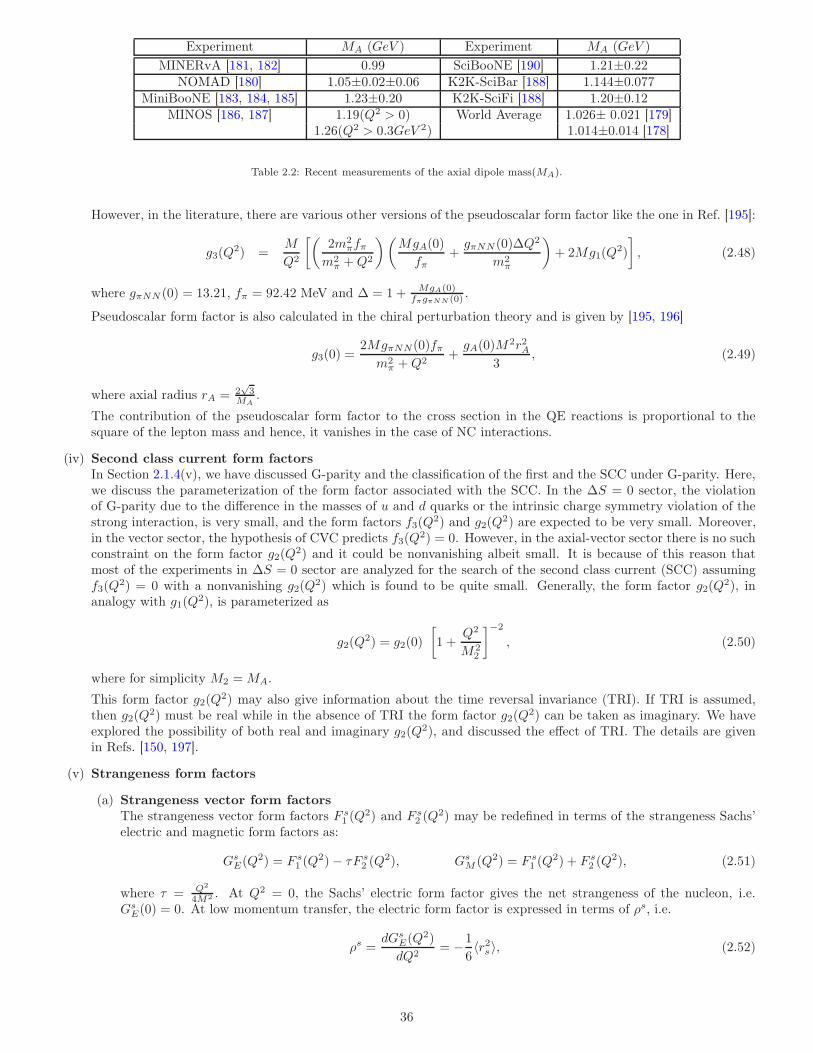
Experiment MA (GeV ) Experiment MA (GeV )

MINERvA [181, 182] 0.99 SciBooNE [190] 1.21±0.22NOMAD [180] 1.05±0.02±0.06 K2K-SciBar [188] 1.144±0.077

MiniBooNE [183, 184, 185] 1.23±0.20 K2K-SciFi [188] 1.20±0.12MINOS [186, 187] 1.19(Q2 > 0) World Average 1.026± 0.021 [179]

1.26(Q2 > 0.3GeV 2) 1.014±0.014 [178]

Table 2.2: Recent measurements of the axial dipole mass(MA).

However, in the literature, there are various other versions of the pseudoscalar form factor like the one in Ref. [195]:

g3(Q2) =

M

Q2

[(

2m2πfπ

m2π +Q2

)(

MgA(0)

fπ+gπNN(0)∆Q2

m2π

)

+ 2Mg1(Q2)

]

, (2.48)

where gπNN (0) = 13.21, fπ = 92.42 MeV and ∆ = 1 + MgA(0)fπgπNN (0) .

Pseudoscalar form factor is also calculated in the chiral perturbation theory and is given by [195, 196]

g3(0) =2MgπNN(0)fπm2

π +Q2+gA(0)M

2r2A3

, (2.49)

where axial radius rA = 2√3

MA.

The contribution of the pseudoscalar form factor to the cross section in the QE reactions is proportional to thesquare of the lepton mass and hence, it vanishes in the case of NC interactions.

(iv) Second class current form factorsIn Section 2.1.4(v), we have discussed G-parity and the classification of the first and the SCC under G-parity. Here,we discuss the parameterization of the form factor associated with the SCC. In the ∆S = 0 sector, the violationof G-parity due to the difference in the masses of u and d quarks or the intrinsic charge symmetry violation of thestrong interaction, is very small, and the form factors f3(Q

2) and g2(Q2) are expected to be very small. Moreover,

in the vector sector, the hypothesis of CVC predicts f3(Q2) = 0. However, in the axial-vector sector there is no such

constraint on the form factor g2(Q2) and it could be nonvanishing albeit small. It is because of this reason that

most of the experiments in ∆S = 0 sector are analyzed for the search of the second class current (SCC) assumingf3(Q

2) = 0 with a nonvanishing g2(Q2) which is found to be quite small. Generally, the form factor g2(Q

2), inanalogy with g1(Q

2), is parameterized as

g2(Q2) = g2(0)

[

1 +Q2

M22

]−2

, (2.50)

where for simplicity M2 =MA.

This form factor g2(Q2) may also give information about the time reversal invariance (TRI). If TRI is assumed,

then g2(Q2) must be real while in the absence of TRI the form factor g2(Q

2) can be taken as imaginary. We haveexplored the possibility of both real and imaginary g2(Q

2), and discussed the effect of TRI. The details are givenin Refs. [150, 197].

(v) Strangeness form factors

(a) Strangeness vector form factorsThe strangeness vector form factors F s

1 (Q2) and F s

2 (Q2) may be redefined in terms of the strangeness Sachs’

electric and magnetic form factors as:

GsE(Q

2) = F s1 (Q

2)− τF s2 (Q

2), GsM (Q2) = F s

1 (Q2) + F s

2 (Q2), (2.51)

where τ = Q2

4M2 . At Q2 = 0, the Sachs’ electric form factor gives the net strangeness of the nucleon, i.e.Gs

E(0) = 0. At low momentum transfer, the electric form factor is expressed in terms of ρs, i.e.

ρs =dGs

E(Q2)

dQ2= −1

6〈r2s 〉, (2.52)

36

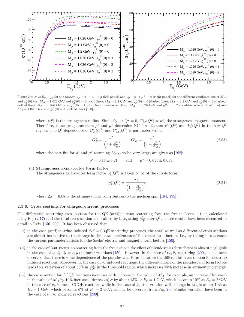
0 0.5 1 1.5 2 2.5 3Eνµ

(GeV)0

20

40

60

80

100

120σ

(10-4

0 cm

2 )

MA

= 1.026 GeV, g2

R (0) = 0

MA

= 1.1 GeV, g2

R (0) = 0

MA

= 1.2 GeV, g2

R (0) = 0

MA

= 1.026 GeV, g2

R (0) = 1

MA

= 1.026 GeV, g2

R (0) = 2

MA

= 1.026 GeV, g2

R (0) = 3

0 0.5 1 1.5 2 2.5 3Eνµ

(GeV)0

20

40

60

80

σ (1

0-40 c

m2 )

MA

= 1.026 GeV, g2

R (0) = 0

MA

= 1.1 GeV, g2

R (0) = 0

MA

= 1.2 GeV, g2

R (0) = 0

MA

= 1.026 GeV, g2

R (0) = 1

MA

= 1.026 GeV, g2

R (0) = 2

Figure 2.6: σ vs Eνµ(νµ) for the process νµ + n → µ− + p (left panel) and νµ + p → µ+ + n (right panel) for the different combinations of MA,

and gR2 (0) viz. MA = 1.026 GeV and gR2 (0) = 0 (solid line), MA = 1.1 GeV and gR2 (0) = 0 (dashed line), MA = 1.2 GeV and gR2 (0) = 0 (dashed-dotted line), MA = 1.026 GeV and gR2 (0) = 1 (double-dotted-dashed line), MA = 1.026 GeV and gR2 (0) = 2 (double-dashed-dotted line) andMA = 1.026 GeV and gR2 (0) = 3 (dotted line) [150].

where 〈r2s〉 is the strangeness radius. Similarly, at Q2 = 0, GsM (Q2) = µs, the strangeness magnetic moment.

Therefore, these two parameters ρs and µs determine NC form factors F s1 (Q

2) and F s2 (Q

2) in the low Q2

region. The Q2 dependence of GsE(Q

2) and GsM (Q2) is parameterized as:

GsE =

ρsτ(

1 + Q2

Λ2E

) , GsM =

µs

(

1 + Q2

Λ2M

) , (2.53)

where the best fits for ρs and µs assuming ΛsE,M to be very large, are given as [198]:

ρs = 0.13± 0.21 and µs = 0.035± 0.053.

(a) Strangeness axial-vector form factorThe strangeness axial-vector form factor gs1(Q

2) is taken to be of the dipole form:

gs1(Q2) =

∆s(

1 + Q2

M2A

)2 (2.54)

where ∆s = 0.08 is the strange quark contribution to the nucleon spin [184, 199].

2.1.6. Cross sections for charged current processes

The differential scattering cross section for the QE (anti)neutrino scattering from the free nucleons is then calculatedusing Eq. (2.17) and the total cross section is obtained by integrating dσ

dQ2 over Q2. These results have been discussed in

detail in Refs. [150, 200]. It has been observed that

(i) in the case (anti)neutrino induced ∆S = 0 QE scattering processes, the total as well as differential cross sectionsare almost insensitive to the change in the parameterization of the vector form factors, i.e., by taking into accountthe various parameterizations for the Sachs’ electric and magnetic form factors [150].

(ii) in the case of (anti)neutrino scattering from the free nucleon the effect of pseudoscalar form factor is almost negligiblein the case of νl, νl; (l = e, µ) induced reactions [150]. However, in the case of ντ , ντ scattering [200], it has beenobserved that there is some dependence of the pseudoscalar form factor on the differential cross section for neutrinoinduced reactions. Moreover, in the case of ντ induced reactions, the different choice of the pseudoscalar form factorsleads to a variation of about 50% in dσ

dQ2 in the threshold region which increases with increase in antineutrino energy.

(iii) the cross section for CCQE reactions increases with increase in the value of MA, for example, an increase (decrease)in the value of MA by 10% increases (decreases) σ by about 15% at Eν = 1 GeV, which becomes 10% at Eν = 2 GeVin the case of νµ induced CCQE reactions while in the case of νµ, the vriation with change in MA is about 10% atEν = 1 GeV, which becomes 6% at Eν = 2 GeV, as may be observed from Fig. 2.6. Similar variation have been inthe case of ντ , ντ induced reactions [200].

37

(iv) the presence of SCC form factors g2(Q2) increases the cross sections for both neutrino and antineutrino induced

processes.

Since the cross section for CCQE processes is sensitive to both MA and g2(Q2), therefore, the dependence of the total

scattering cross section on MA is shown in Fig. 2.6 by varying MA in the range 1.026–1.2 GeV, with or without thepresence of SCC by varying gR2 (0) in the range 0− 3, using the BBBA05 [160] parameterization of the Sachs’ electric andmagnetic form factors. It may be observed from the figure that:

(a) in the absence of SCC (gR2 (0) = 0) [150], the cross section for both neutrino and antineutrino induced reactionsincreases with increase in the value of MA as discussed above.

(b) for the process νµ + n −→ µ− + p, the results obtained by taking MA = 1.1 GeV and gR2 (0) = 0 are comparable tothe results obtained with MA = 1.026 GeV and gR2 (0) = 2, whereas the results obtained by taking MA = 1.2 GeVand gR2 (0) = 0 are comparable to the results obtained using MA = 1.026 GeV and gR2 (0) = 3.

(c) for the process νµ + p −→ µ+ + n, the results obtained by taking MA = 1.1 GeV and gR2 (0) = 0 are comparable tothe results obtained with MA = 1.026 GeV and gR2 (0) = 1, whereas the results obtained by taking MA = 1.2 GeVand gR2 (0) = 0 are slightly lower than the results obtained using MA = 1.026 GeV and gR2 (0) = 2. Thus, a highervalue of σ(Eνµ ) may be obtained by either taking a nonzero value of g2(0) or increasing the value of MA.

(d) The cross section measurements may give information only about the nonzero value of g2(0) irrespective of thenature of the SCC current i.e. with or without time reversal invariance.

However, one may obtain the nature of the SCC by measuring the polarization observables which gives different resultswith the real and imaginary values of g2(0), corresponding to the SCC with or without time reversal invariance, and thishas been discussed by us in brief in Section 2.3. For more discussion, readers are referred to Fatima et al. [150, 200].

2.2. Quasielastic hyperon production

The following processes are induced when an antineutrino interacts with a nucleon to produce a hyperon and an antilep-ton (Fig. 2.7):

νl(k) + p(p) → l+(k′) + Λ/Σ0(p′), (2.55)

νl(k) + n(p) → l+(k′) + Σ−(p′); l = e, µ, τ, (2.56)

where the quantities in the brackets represent the four momenta of the particles.

2.2.1. Matrix elements and form factors

The transition matrix element for the processes presented in Eqs. (2.55)–(2.56) is written as

M =GF√2sin θc l

µJµ. (2.57)

The leptonic current (lµ) is given in Eq. (2.10). The hadronic current (Jµ) for the QE hyperon production can be writtenin analogy with the antineutrino-nucleon scattering except that the mass of the final nucleon is replaced by the mass ofthe hyperon and the electroweak form factors of the nucleons are replaced by the N − Y transition form factors. Thegeneral expression for Jµ is given in Eq. (2.11) and the matrix elements of the vector (Vµ) and the axial-vector (Aµ)currents between a hyperon Y (= Λ,Σ0 and Σ−) and a nucleon N = n, p are written as:

〈Y (~p ′)|Vµ|N(~p)〉 = u(~p ′)

[

γµfNY1 (Q2) + iσµν

qν

M +M ′ fNY2 (Q2)

2 qµM +M ′ f

NY3 (Q2)

]

u(~p), (2.58)

〈Y (~p ′)|Aµ|N(~p)〉 = u(~p ′)

[

γµγ5gNY1 (Q2) + iσµν

qν

M +M ′ γ5gNY2 (Q2)

2 qµM +M ′ γ5g

NY3 (Q2)

]

u(~p), (2.59)

where M and M ′ are the masses of the nucleon and hyperon, respectively. fNY1 (Q2), fNY

2 (Q2) and fNY3 (Q2) are the

vector, weak magnetic and induced scalar N − Y transition form factors and gNY1 (Q2), gNY

2 (Q2) and gNY3 (Q2) are the

axial-vector, induced tensor (or weak electric) and induced pseudoscalar form factors, respectively.The transition matrix element squared is obtained as

∑∑

|M|2 =G2

F sin2 θc2

JµνLµν , (2.60)

where Jµν and Lµν are obtained in a similar way, as mentioned in Section 2.1.2.

38

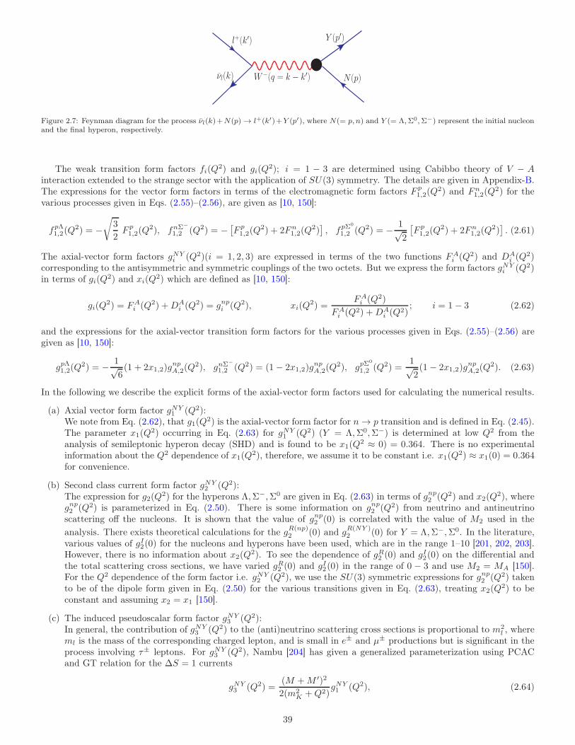
νl(k)

l+(k′)

W−(q = k − k′)

Y (p′)

N(p)

Figure 2.7: Feynman diagram for the process νl(k)+N(p) → l+(k′)+Y (p′), where N(= p, n) and Y (= Λ,Σ0,Σ−) represent the initial nucleonand the final hyperon, respectively.

The weak transition form factors fi(Q2) and gi(Q

2); i = 1 − 3 are determined using Cabibbo theory of V − Ainteraction extended to the strange sector with the application of SU(3) symmetry. The details are given in Appendix-B.The expressions for the vector form factors in terms of the electromagnetic form factors F p

1,2(Q2) and Fn

1,2(Q2) for the

various processes given in Eqs. (2.55)–(2.56), are given as [10, 150]:

fpΛ1,2(Q

2) = −√

3

2F p1,2(Q

2), fnΣ−

1,2 (Q2) = −[

F p1,2(Q

2) + 2Fn1,2(Q

2)]

, fpΣ0

1,2 (Q2) = − 1√2

[

F p1,2(Q

2) + 2Fn1,2(Q

2)]

. (2.61)

The axial-vector form factors gNYi (Q2)(i = 1, 2, 3) are expressed in terms of the two functions FA

i (Q2) and DAi (Q

2)corresponding to the antisymmetric and symmetric couplings of the two octets. But we express the form factors gNY

i (Q2)in terms of gi(Q

2) and xi(Q2) which are defined as [10, 150]:

gi(Q2) = FA

i (Q2) +DAi (Q

2) = gnpi (Q2), xi(Q2) =

FAi (Q2)

FAi (Q2) +DA

i (Q2); i = 1− 3 (2.62)

and the expressions for the axial-vector transition form factors for the various processes given in Eqs. (2.55)–(2.56) aregiven as [10, 150]:

gpΛ1,2(Q2) = − 1√

6(1 + 2x1,2)g

npA,2(Q

2), gnΣ−

1,2 (Q2) = (1− 2x1,2)gnpA,2(Q

2), gpΣ0

1,2 (Q2) =1√2(1− 2x1,2)g

npA,2(Q

2). (2.63)

In the following we describe the explicit forms of the axial-vector form factors used for calculating the numerical results.

(a) Axial vector form factor gNY1 (Q2):

We note from Eq. (2.62), that g1(Q2) is the axial-vector form factor for n→ p transition and is defined in Eq. (2.45).

The parameter x1(Q2) occurring in Eq. (2.63) for gNY

1 (Q2) (Y = Λ,Σ0,Σ−) is determined at low Q2 from theanalysis of semileptonic hyperon decay (SHD) and is found to be x1(Q

2 ≈ 0) = 0.364. There is no experimentalinformation about the Q2 dependence of x1(Q

2), therefore, we assume it to be constant i.e. x1(Q2) ≈ x1(0) = 0.364

for convenience.

(b) Second class current form factor gNY2 (Q2):

The expression for g2(Q2) for the hyperons Λ,Σ−,Σ0 are given in Eq. (2.63) in terms of gnp2 (Q2) and x2(Q

2), wheregnp2 (Q2) is parameterized in Eq. (2.50). There is some information on gnp2 (Q2) from neutrino and antineutrinoscattering off the nucleons. It is shown that the value of gnp2 (0) is correlated with the value of M2 used in the

analysis. There exists theoretical calculations for the gR(np)2 (0) and g

R(NY )2 (0) for Y = Λ,Σ−,Σ0. In the literature,

various values of gI2(0) for the nucleons and hyperons have been used, which are in the range 1–10 [201, 202, 203].However, there is no information about x2(Q

2). To see the dependence of gR2 (0) and gI2(0) on the differential andthe total scattering cross sections, we have varied gR2 (0) and gI2(0) in the range of 0 − 3 and use M2 = MA [150].For the Q2 dependence of the form factor i.e. gNY

2 (Q2), we use the SU(3) symmetric expressions for gnp2 (Q2) takento be of the dipole form given in Eq. (2.50) for the various transitions given in Eq. (2.63), treating x2(Q

2) to beconstant and assuming x2 = x1 [150].

(c) The induced pseudoscalar form factor gNY3 (Q2):

In general, the contribution of gNY3 (Q2) to the (anti)neutrino scattering cross sections is proportional to m2

l , whereml is the mass of the corresponding charged lepton, and is small in e± and µ± productions but is significant in theprocess involving τ± leptons. For gNY

3 (Q2), Nambu [204] has given a generalized parameterization using PCACand GT relation for the ∆S = 1 currents

gNY3 (Q2) =

(M +M ′)2

2(m2K +Q2)

gNY1 (Q2), (2.64)

39

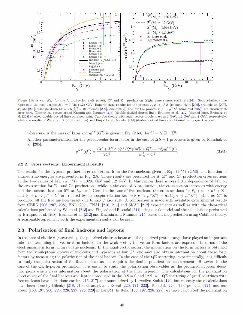
0 2 4 6 8Eν µ

(GeV)0

0.5

1

1.5

2

2.5

3

3.5

σ (

10

-40 c

m2 )

Erriquez et al.Eichten et al.Brunner et al. Brunner et al.Erriquez et al.Erriquez et al.Our Result (M

A=1.026 GeV)

Wu et al. (x 3) Finjord et al.Fanourakis et al.Kuzmin et al.Our result (M

A = 1.2 GeV)

0 2 4 6 8 10 12 14Eν µ

(GeV)0

0.5

1

1.5

2

2.5

σ (

×10

-40 c

m2)

Σ0 (M

A = 1.026 GeV)

Σ0 (M

A = 1.2 GeV)

Σ− (M

A = 1.026 GeV)

Σ− (M

A = 1.2 GeV)

Erriquez et al.Ammosov et al.

Figure 2.8: σ vs. Eνµ for the Λ production (left panel), Σ0 and Σ− production (right panel) cross sections [197]. Solid (dashed) line

represents the result using MA = 1.026 (1.2) GeV. Experimental results for the process νµp → µ+Λ (triangle right [206], triangle up [207],

square [208], triangle down (σ = 2.6+5.9−2.1 × 10−40cm2) [209], circle [212]) and for the process νµp → µ+Σ0 (diamond [207]) are shown with

error bars. Theoretical curves are of Kuzmin and Naumov [215] (double dashed-dotted line), Brunner et al. [212] (dashed line), Erriquez etal. [208] (dashed-double dotted line) obtained using Cabibbo theory with axial-vector dipole mass as 1 GeV, 1.1 GeV and 1 GeV, respectively,while the results of Wu et al. [213] (dotted line) and Finjord and Ravndal [214] (dashed dotted line) are obtained using quark model.

where mK is the mass of kaon and gNY1 (Q2) is given in Eq. (2.63), for Y = Λ,Σ−,Σ0.

Another parameterization for the pseudoscalar form factor in the case of ∆S = 1 processes is given by Marshak etal. [205]:

gNY3 (Q2) =

(M +M ′)2

2Q2

gNY1 (Q2)(m2

K +Q2)−m2Kg

NY1 (0)

m2K +Q2

. (2.65)

2.2.2. Cross sections: Experimental results

The results for the hyperon production cross sections from the free nucleons given in Eqs. (2.55)–(2.56) as a function ofantineutrino energies are presented in Fig. 2.8. These results are presented for Λ, Σ− and Σ0 production cross sectionsat the two values of MA viz. MA = 1.026 GeV and 1.2 GeV. In this region there is very little dependence of MA onthe cross section for Σ− and Σ0 productions, while in the case of Λ production, the cross section increases with energyand the increase is about 5% at Eνµ = 1 GeV. In the case of free nucleon, the cross sections for νµ + n → µ+ + Σ−

and νµ + p → µ+ + Σ0 are related by an isospin relation i.e. σ(νµp → µ+Σ0) = 12σ(νµn → µ+Σ−), while no Σ+ is

produced off the free nucleon target due to ∆S 6= ∆Q rule. A comparison is made with available experimental resultsfrom CERN [206, 207, 208], BNL [209], FNAL [210, 211] and SKAT [212] experiments as well as with the theoreticalcalculations performed by Wu et al. [213] and Finjord and Ravndal [214] using quark model and the calculations performedby Erriquez et al. [208], Brunner et al. [212] and Kuzmin and Naumov [215] based on the prediction using Cabibbo theory.A reasonable agreement with the experimental results can be seen.

2.3. Polarization of final hadrons and leptons

In the case of elastic e−p scattering, the polarized electron beam and the polarized proton target have played an importantrole in determining the vector form factors. In the weak sector, the vector form factors are expressed in terms of theelectromagnetic form factors of the nucleons. In the axial-vector sector, the information on the form factors is obtainedform the semileptonic decays of nucleons and hyperons at low Q2, one may also obtain information about these formfactors by measuring the polarization of the final hadron. In the case of the QE scattering, experimentally, it is difficultto study the polarization of the final nucleon as one requires the double polarization measurement. However, in thecase of the QE hyperon production, it is easier to study the polarization observables as the produced hyperon decayinto pions which gives information about the polarization of the final hyperon. The calculations for the polarizationobservables of the final hadrons and leptons produced in the ∆S = 0 and |∆S| = 1 QE scattering of (anti)neutrinos withfree nucleons have been done earlier [216, 217] and summarized by Llewellyn Smith [149] but recently these calculationshave been done by Bilenky [218, 219], Graczyk and Kowal [220, 221, 222], Tomalak [223], Thorpe et al. [224] and ourgroup [150, 197, 200, 225, 226, 227, 228, 229] in the SM. In Refs. [150, 197, 226, 227], we have calculated the polarization

40

observables of the proton, neutron, Λ, Σ− produced in the νµ induced QE processes. In Refs. [200, 228], we have studiedthe τ± polarization in the processes ντ (ντ ) +N −→ τ± +N and ντ +N −→ τ+ + Λ(Σ).

2.3.1. Polarization of the final hadron

The polarization 4-vector ξτ of the hadron produced in the final state in reactions (2.5), (2.55)–(2.56) is written as [10, 230]:

ξτ =Tr[γτγ5 ρf (p

′)]

Tr[ρf (p′)], (2.66)

where the spin density matrix ρf (p′) corresponding to the final hadron of momentum p′ is given by

ρf (p′) = Lαβ Tr[Λ(p′)OαΛ(p)OβΛ(p

′)], (2.67)

where Λ(p′) = /p′ +M ′ is the projection operator for spin 12 fermions with momentum p′.

Using the following relations:

Λ(p′)γτγ5Λ(p′) = 2M ′

(

gτσ − p′τp′σ

M ′2

)

Λ(p′)γσγ5, Λ(p′)Λ(p′) = 2M ′Λ(p′), (2.68)

where M ′ corresponds to the mass of the final hadron. ξτ defined in Eq. (2.66) may be rewritten as [10, 230]:

ξτ =

(

gτσ − p′τp′σ

M ′2

) LαβTr[

γσγ5Λ(p′)OαΛ(p)Oβ

]

LαβTr[

Λ(p′)OαΛ(p)Oβ

] . (2.69)

Note that in Eq. (2.69), ξτ is manifestly orthogonal to p′τ , i.e. p′ · ξ = 0. Moreover, the denominator is directly related tothe differential scattering cross section given in Eq. (2.17). With Jαβ and Lαβ given in Eqs. (2.16) and (2.15), respectively,an expression for ξτ is obtained in terms of the 4-momenta of the particles. Here, we have considered two cases:

Case I: When time reversal invariance is assumed.The polarization vector ξτ defined in Eq. (2.69) is evaluated in the laboratory frame, i.e. when the initial nucleon is

at rest, ~p = 0, and the momentum directions are depicted in Fig. 2.9(a). If the time reversal invariance is assumed thenall the form factors defined in Eqs. (2.12), (2.13), (2.58), and (2.59) are real and ξτ is expressed as

~ξ =

[

Ah(Q2)~k +Bh(Q2)~p ′]

N(Q2), (2.70)

where the expressions of Ah(Q2), Bh(Q2) and N(Q2) are given in Appendix-A.1. In Eq. (2.70), Ah(Q2), Bh(Q2) andN(Q2) given in Appendix-A.1 are taken in the limit f3(Q

2) = 0 and g2(0) = gR2 (0) to ensure the time reversal invariance.

From Eq. (2.70), it follows that the polarization vector lies in the plane of reaction and there is no component ofpolarization in a direction perpendicular to the reaction plane. This is a consequence of time reversal invariance whichmakes the transverse component of polarization, perpendicular to the reaction plane, to vanish. We now expand ~ξ alongthe orthogonal directions, ehL, ehP and ehT in the reaction plane corresponding to the longitudinal, perpendicular andtransverse directions, defined as

ehL =~p ′

|~p ′| , ehP = ehL × ehT , where ehT =~p ′ × ~k|~p ′ × ~k|

, (2.71)

and have depicted in Fig. 2.9(b). We then write ~ξ as:

~ξ = ξLehL + ξP e

hP , (2.72)

such that the longitudinal and perpendicular components of ~ξ in the laboratory frame are given by

ξL(Q2) = ~ξ · ehL, ξP (Q

2) = ~ξ · ehP . (2.73)

From Eq. (2.73), the longitudinal P hL(Q

2) and perpendicular P hP (Q

2) components of the ~ξ defined in the rest frame of thefinal hadron are given by

P hL(Q

2) =M ′

Ep′

ξL(Q2), P h

P (q2) = ξP (Q

2), (2.74)

41

x

z

yX(~p ′)

νµ(~k)

µ+(~k ′)

ehL

ehTehP elLelT

elP

(a) (c)(b)

Figure 2.9: (a) Momentum and polarization directions of the final baryon and the lepton. eh,lL , eh,lP and eh,lT represent the orthogonal unitvectors corresponding to the longitudinal, perpendicular and transverse directions with respect to the momentum of the final hadron in (b)and the final lepton in (c).

where M ′

Ep′is the Lorentz boost factor along ~p ′. With the help of Eqs. (2.70), (2.71), (2.73) and (2.74), the longitudinal

P hL(Q

2) and perpendicular P hP (Q

2) components of polarization are calculated to be [10, 150]:

P hL(Q

2) =M ′

Ep′

Ah(Q2)~k · ~p ′ +Bh(Q2)|~p ′|2N(Q2) |~p ′| , (2.75)

P hP (Q

2) =Ah(Q2)[(~k · ~p ′)2 − |~k|2|~p ′|2]

N(Q2) |~p ′| |~p ′ × ~k|. (2.76)

Case II: When time reversal violation is assumed.In the absence of time reversal invariance, ~ξ is calculated as [10, 150]

~ξ =Ah(Q2)~k +Bh(Q2)~p ′ + Ch(Q2)M(~k × ~p ′)

N(Q2). (2.77)

where the expressions of Ch(Q2) is given in Appendix-A.1.

The ~ξ may be written in terms of the longitudinal, perpendicular and transverse components as

~ξ = ξLehL + ξP e

hP + ξT e

hT , (2.78)

where the unit vectors are defined in Eq. (2.71). The longitudinal and perpendicular components are given in Eqs. (2.75)and (2.76), respectively. The transverse component of polarization in the rest frame of the final hadron is given as

PT (Q2) = ξT (Q

2) = ~ξ.eT . (2.79)

Using Eqs. (2.71) and (2.78) in Eq. (2.79), we obtain [10, 150]

P hT (Q

2) =Ch(Q2)M [(~k · ~p ′)2 − |~k|2|~p ′|2]

N(Q2) |~p ′ × ~k|. (2.80)

If the T invariance is assumed then all the vector and the axial-vector form factors are real and the expression for Ch(Q2)vanishes which implies that the transverse component of the polarization perpendicular to the production plane, P h

T (Q2)

vanishes.Using Eqs. (2.75), (2.76) and (2.80), the polarization components of the Λ produced in the reaction νµ+p −→ µ++Λ

are calculated, where the expressions of Ah(Q2), Bh(Q2), and Ch(Q2) are given in Appendix A.1. To see the dependenceof gR2 (0) on the polarization observables, in Fig. 2.10, the results of PL(Q

2) and PP (Q2) are presented as a function of

Q2 using gR2 (0) = 0, ±1 and ±3 at Eνµ = 1 GeV. It may be observed that PL(Q2) shows large variations as we change

|gR2 (0)| from 0 to 3. For example, in the peak region of Q2, the difference is about 50% as |gR2 (0)| is changed from 0 to 3.In the case of PP (Q

2), Q2 dependence is quite strong and similar to PL(Q2).

42

0 0.2 0.4 0.6 0.8 1

Q2 (GeV

2)

-1

-0.5

0

0.5

1

PL

Λ (

Q2 )

Eνµ = 1 GeV

0 0.2 0.4 0.6 0.8 1

Q2 (GeV

2)

-1

-0.8

-0.6

-0.4

-0.2

0

0.2

0.4

PP

Λ (

Q2 ) Eνµ

= 1 GeV

Figure 2.10: PL(Q2) vs. Q2 (left panel) and PP (Q2) vs. Q2 (right panel) for the process νµ + p → µ+ + Λ at the incoming antineutrino energy,

Eνµ = 1 GeV for the polarized Λ in the final state, at the different values of gR2 (0) viz. gR2 (0) = 0 (solid line), 1 (dashed line), 3 (dashed-dottedline), −1 (double-dotted-dashed line) and −3 (double-dashed-dotted line) [150].

0 0.2 0.4 0.6 0.8 1

Q2 (GeV

2)

0

0.2

0.4

0.6

0.8

PL

Λ (

Q2)

Eνµ = 1 GeV

0 0.2 0.4 0.6 0.8 1

Q2 (GeV

2)

-1

-0.8

-0.6

-0.4

-0.2

0

0.2

PP

Λ (

Q2)

Eνµ = 1 GeV

0 0.2 0.4 0.6 0.8 1

Q2 (GeV

2)

-0.4

-0.2

0

0.2

0.4

PT

Λ (

Q2)

Eνµ = 1 GeV

Figure 2.11: PL(Q2) vs. Q2 (left panel), PP (Q2) vs. Q2 (middle panel) and PT (Q2) vs. Q2 (right panel) for the process νµ + p → µ+ + Λ at

the incoming antineutrino energy, Eνµ = 1 GeV for the polarized Λ in the final state, at the different values of gI2(0) viz. gI2(0) = 0 (solid line),1 (dashed line) and 3 (dashed-dotted line) [150].

43

To see the dependence of gI2(0) on the polarization observables, in Fig. 2.11, the results are presented for PL(Q2),

PP (Q2) and PT (Q

2) as a function of Q2 using gI2(0) = 0, 1 and 3 at Eνµ = 1 GeV. It may be deduced that while PL(Q2)

is less sensitive to gI2(0) at low antineutrino energies, PP (Q2) is sensitive to gI2(0) at Eνµ = 1 GeV. Moreover, PT (Q

2)shows 40% variations at Q2 = 0.4 GeV2, Eνµ = 1 GeV, when gI2(0) is varied from 0 to 3.

2.3.2. Polarization of the final lepton

In the case of final lepton polarization in CC reactions, the polarization 4-vector (ζτ ) in reactions (2.5), (2.55)–(2.56) iswritten as [10, 150]:

ζτ =Tr[γτγ5 ρf (k

′)]

Tr[ρf (k′)], (2.81)

and the spin density matrix for the final lepton ρf (k′) is given by

ρf (k′) = Jαβ Tr[Λ(k′)γα(1 + γ5)Λ(k)γβ(1 + γ5)Λ(k

′)], (2.82)

with γα = γ0γ†αγ0 and γ5 = γ0γ†5γ

0.Using Eq. (2.68), ζτ defined in Eq. (2.81) may also be rewritten as [10, 150]

ζτ =

(

gτσ − k′τk′σ

m2l

)

JαβTr [γσγ5Λ(k′)γα(1 + γ5)Λ(k)γβ(1 + γ5)]

JαβTr [Λ(k′)γα(1 + γ5)Λ(k)γβ(1 + γ5)], (2.83)

where ml is the charged lepton mass.With Jαβ and Lαβ given in Eqs. (2.16) and (2.15), respectively, an expression for ζτ is obtained. In the laboratory

frame where the initial nucleon is at rest, the polarization vector ~ζ is calculated to be a function of 3-momenta of incomingantineutrino (~k) and outgoing lepton (~k ′), and is given as [10, 150]

~ζ =

[

Al(Q2)~k +Bl(Q2)~k ′ + Cl(Q2)M(~k × ~k ′)]

N(Q2), (2.84)

where the expressions of Al(Q2), Bl(Q2) and Cl(Q2) are given in Appendix-A.2.

One may expand ~ζ along the orthogonal directions, elL, elP and elT in the reaction plane corresponding to the longitu-dinal, perpendicular and transverse directions, defined as

elL =~k ′

|~k ′|, elP = elL × elT , where elT =

~k × ~k ′

|~k × ~k ′|, (2.85)

and depicted in Fig. 2.9(c). We then ~ζ as:~ζ = ζLe

lL + ζP e

lP + ζT e

lT , (2.86)

such that the longitudinal, perpendicular and transverse components of the ~ζ in the laboratory frame are given by

ζL(Q2) = ~ζ · elL, ζP (Q

2) = ~ζ · elP , ζT (Q2) = ~ζ · elT . (2.87)

From Eq. (2.87), the longitudinal P lL(Q

2), perpendicular P lP (Q

2) and transverse P lT (Q

2) components of ~ζ defined in therest frame of the final lepton are given by

P lL(Q

2) =ml

Ek′

ζL(Q2), P l

P (Q2) = ζP (Q

2), P lT (Q

2) = ζT (Q2), (2.88)

where ml

Ek′is the Lorentz boost factor along ~k ′. Using Eqs. (2.84), (2.85) and (2.87) in Eq. (2.88), the longitudinal P l

L(Q2),

perpendicular P lP (Q

2) and transverse P lT (Q

2) components of lepton polarization are calculated to be [10, 150]

P lL(Q

2) =ml

Ek′

Al(Q2)~k · ~k ′ + Bl(Q2)|~k ′|2

N(Q2) |~k ′|, (2.89)

P lP (Q

2) =Al(Q2)[|~k|2|~k ′|2 − (~k · ~k ′)2]

N(Q2) |~k ′| |~k × ~k ′|, (2.90)

P lT (Q

2) =Cl(Q2)M [(~k · ~k ′)2 − |~k|2|~k ′|2]

N(Q2) |~k × ~k ′|. (2.91)

Using Eqs. (2.17), (2.89), (2.90), (2.91) the differential scattering cross section as well as the polarization observablesof the final lepton produced in the (anti)neutrino induced processes are calculated. It has been observed that

44

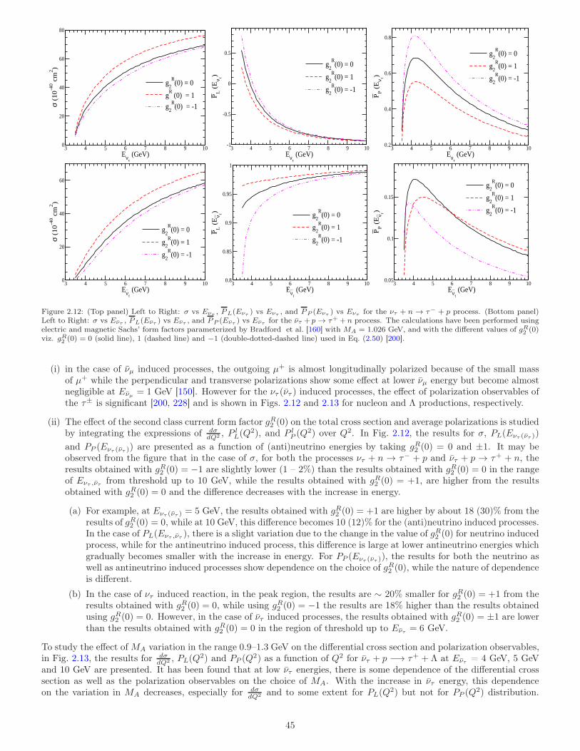
3 4 5 6 7 8 9 10Eντ

(GeV)0

20

40

60

80

σ (

10-4

0 cm

2 )

g2

R(0) = 0

gR (0) = 1

g2

R(0) = -1

3 4 5 6 7 8 9 10Eντ

(GeV)-1

-0.5

0

0.5

PL (

Eν τ)

g2

R(0) = 0

g2

R(0) = 1

g2

R(0) = -1

3 4 5 6 7 8 9 10Eντ

(GeV)0.2

0.4

0.6

0.8

PP (

Eν τ)

g2

R(0) = 0

g2

R(0) = 1

g2

R(0) = -1

3 4 5 6 7 8 9 10Eντ

(GeV)0

20

40

60

σ (

10-4

0 cm

2 )

g2

R(0) = 0

g2

R(0) = 1

g2

R(0) = -1

3 4 5 6 7 8 9 10Eντ

(GeV)0.8

0.85

0.9

0.95

1

PL (

Eν τ) g

2

R(0) = 0

g2

R(0) = 1

g2

R(0) = -1

3 4 5 6 7 8 9 10Eντ

(GeV)0.05

0.1

0.15

PP (

Eν τ)

g2

R(0) = 0

g2

R(0) = 1

g2

R(0) = -1

Figure 2.12: (Top panel) Left to Right: σ vs Eντ , PL(Eντ ) vs Eντ , and PP (Eντ ) vs Eντ for the ντ + n → τ− + p process. (Bottom panel)Left to Right: σ vs Eντ , PL(Eντ ) vs Eντ , and PP (Eντ ) vs Eντ for the ντ + p → τ+ +n process. The calculations have been performed usingelectric and magnetic Sachs’ form factors parameterized by Bradford et al. [160] with MA = 1.026 GeV, and with the different values of gR2 (0)viz. gR2 (0) = 0 (solid line), 1 (dashed line) and −1 (double-dotted-dashed line) used in Eq. (2.50) [200].

(i) in the case of νµ induced processes, the outgoing µ+ is almost longitudinally polarized because of the small massof µ+ while the perpendicular and transverse polarizations show some effect at lower νµ energy but become almostnegligible at Eνµ = 1 GeV [150]. However for the ντ (ντ ) induced processes, the effect of polarization observables ofthe τ± is significant [200, 228] and is shown in Figs. 2.12 and 2.13 for nucleon and Λ productions, respectively.

(ii) The effect of the second class current form factor gR2 (0) on the total cross section and average polarizations is studiedby integrating the expressions of dσ

dQ2 , P lL(Q

2), and P lP (Q

2) over Q2. In Fig. 2.12, the results for σ, PL(Eντ (ντ ))

and PP (Eντ (ντ )) are presented as a function of (anti)neutrino energies by taking gR2 (0) = 0 and ±1. It may beobserved from the figure that in the case of σ, for both the processes ντ + n → τ− + p and ντ + p → τ+ + n, theresults obtained with gR2 (0) = −1 are slightly lower (1 – 2%) than the results obtained with gR2 (0) = 0 in the rangeof Eντ ,ντ from threshold up to 10 GeV, while the results obtained with gR2 (0) = +1, are higher from the resultsobtained with gR2 (0) = 0 and the difference decreases with the increase in energy.

(a) For example, at Eντ (ντ ) = 5 GeV, the results obtained with gR2 (0) = +1 are higher by about 18 (30)% from theresults of gR2 (0) = 0, while at 10 GeV, this difference becomes 10 (12)% for the (anti)neutrino induced processes.In the case of PL(Eντ ,ντ ), there is a slight variation due to the change in the value of gR2 (0) for neutrino inducedprocess, while for the antineutrino induced process, this difference is large at lower antineutrino energies whichgradually becomes smaller with the increase in energy. For PP (Eντ (ντ )), the results for both the neutrino aswell as antineutrino induced processes show dependence on the choice of gR2 (0), while the nature of dependenceis different.

(b) In the case of ντ induced reaction, in the peak region, the results are ∼ 20% smaller for gR2 (0) = +1 from theresults obtained with gR2 (0) = 0, while using gR2 (0) = −1 the results are 18% higher than the results obtainedusing gR2 (0) = 0. However, in the case of ντ induced processes, the results obtained with gR2 (0) = ±1 are lowerthan the results obtained with gR2 (0) = 0 in the region of threshold up to Eντ = 6 GeV.

To study the effect of MA variation in the range 0.9–1.3 GeV on the differential cross section and polarization observables,in Fig. 2.13, the results for dσ

dQ2 , PL(Q2) and PP (Q

2) as a function of Q2 for ντ + p −→ τ+ + Λ at Eντ = 4 GeV, 5 GeVand 10 GeV are presented. It has been found that at low ντ energies, there is some dependence of the differential crosssection as well as the polarization observables on the choice of MA. With the increase in ντ energy, this dependenceon the variation in MA decreases, especially for dσ

dQ2 and to some extent for PL(Q2) but not for PP (Q

2) distribution.

45

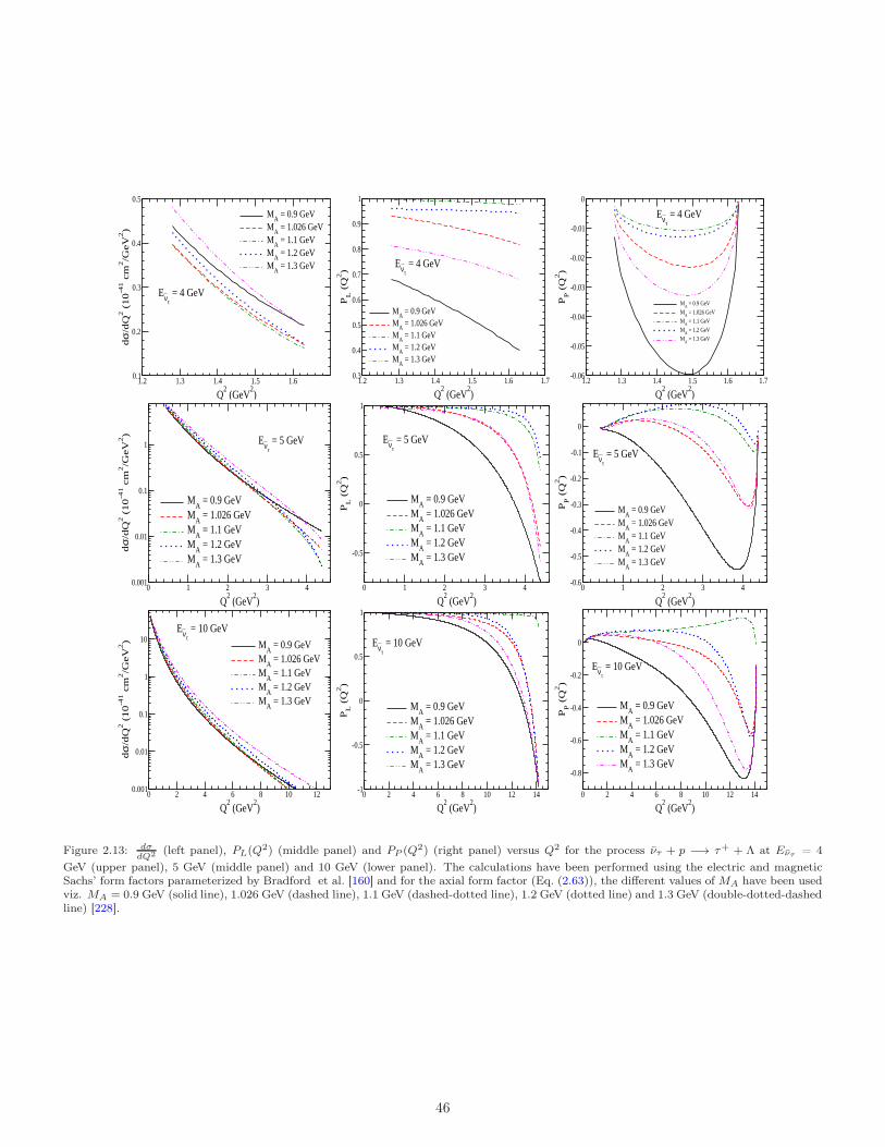
1.2 1.3 1.4 1.5 1.6

Q2 (GeV

2)

0.1

0.2

0.3

0.4

0.5

dσ

/dQ

2 (

10

-41 c

m2/G

eV2)

MA

= 0.9 GeVM

A = 1.026 GeV

MA

= 1.1 GeVM

A = 1.2 GeV

MA

= 1.3 GeV

Eντ = 4 GeV

1.2 1.3 1.4 1.5 1.6 1.7

Q2 (GeV

2)

0.3

0.4

0.5

0.6

0.7

0.8

0.9

1

PL (

Q2)

MA

= 0.9 GeVM

A = 1.026 GeV

MA

= 1.1 GeVM

A = 1.2 GeV

MA

= 1.3 GeV

Eντ = 4 GeV

1.2 1.3 1.4 1.5 1.6 1.7

Q2 (GeV

2)

-0.06

-0.05

-0.04

-0.03

-0.02

-0.01

0

PP (

Q2)

MA

= 0.9 GeV

MA

= 1.026 GeV

MA

= 1.1 GeV

MA

= 1.2 GeV

MA

= 1.3 GeV

Eντ = 4 GeV

0 1 2 3 4

Q2 (GeV

2)

0.001

0.01

0.1

1

dσ

/dQ

2 (

10

-41 c

m2/G

eV2)

MA

= 0.9 GeVM

A = 1.026 GeV

MA

= 1.1 GeVM

A = 1.2 GeV

MA

= 1.3 GeV

Eντ = 5 GeV

0 1 2 3 4

Q2 (GeV

2)

-0.5

0

0.5

1

PL (

Q2)

MA

= 0.9 GeVM

A = 1.026 GeV

MA

= 1.1 GeVM

A = 1.2 GeV

MA

= 1.3 GeV

Eντ = 5 GeV

0 1 2 3 4

Q2 (GeV

2)

-0.6

-0.5

-0.4

-0.3

-0.2

-0.1

0

PP (

Q2)

MA

= 0.9 GeVM

A = 1.026 GeV

MA

= 1.1 GeVM

A = 1.2 GeV

MA

= 1.3 GeV

Eντ = 5 GeV

0 2 4 6 8 10 12

Q2 (GeV

2)

0.001

0.01

0.1

1

10

dσ

/dQ

2 (

10

-41 c

m2/G

eV2) M

A = 0.9 GeV

MA

= 1.026 GeVM

A = 1.1 GeV

MA

= 1.2 GeVM

A = 1.3 GeV

Eντ = 10 GeV

0 2 4 6 8 10 12 14

Q2 (GeV

2)

-1

-0.5

0

0.5

1

PL (

Q2)

MA

= 0.9 GeVM

A = 1.026 GeV

MA

= 1.1 GeVM

A = 1.2 GeV

MA

= 1.3 GeV

Eντ = 10 GeV

0 2 4 6 8 10 12 14

Q2 (GeV

2)

-0.8

-0.6

-0.4

-0.2

0

PP (

Q2)

MA

= 0.9 GeVM

A = 1.026 GeV

MA

= 1.1 GeVM

A = 1.2 GeV

MA

= 1.3 GeV

Eντ = 10 GeV

Figure 2.13: dσdQ2 (left panel), PL(Q

2) (middle panel) and PP (Q2) (right panel) versus Q2 for the process ντ + p −→ τ+ + Λ at Eντ = 4

GeV (upper panel), 5 GeV (middle panel) and 10 GeV (lower panel). The calculations have been performed using the electric and magneticSachs’ form factors parameterized by Bradford et al. [160] and for the axial form factor (Eq. (2.63)), the different values of MA have been usedviz. MA = 0.9 GeV (solid line), 1.026 GeV (dashed line), 1.1 GeV (dashed-dotted line), 1.2 GeV (dotted line) and 1.3 GeV (double-dotted-dashedline) [228].

46

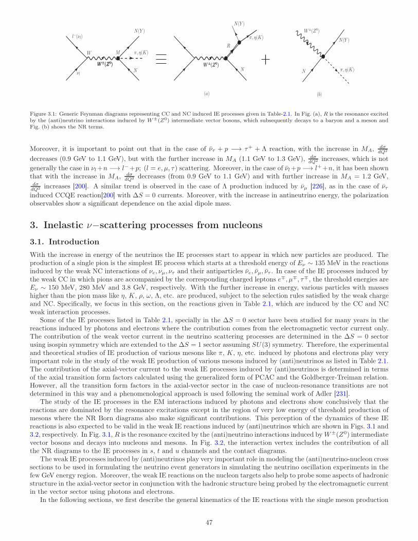
νl

W±(Z0)

W

l−(νl)

M

N

π, η(K)

N(Y )

R

π, η(K)

N(Y )

N N

N(Y )

π, η(K)

(a) (b)

W±(Z0)W±(Z0) W±(Z0)W±(Z0)

W±(Z0)

Figure 3.1: Generic Feynman diagrams representing CC and NC induced IE processes given in Table-2.1. In Fig. (a), R is the resonance excitedby the (anti)neutrino interactions induced by W±(Z0) intermediate vector bosons, which subsequently decays to a baryon and a meson andFig. (b) shows the NR terms.

Moreover, it is important to point out that in the case of ντ + p −→ τ+ + Λ reaction, with the increase in MA, dσdQ2

decreases (0.9 GeV to 1.1 GeV), but with the further increase in MA (1.1 GeV to 1.3 GeV), dσdQ2 increases, which is not

generally the case in νl+n −→ l−+p; (l = e, µ, τ) scattering. Moreover, in the case of νl+p −→ l++n, it has been shownthat with the increase in MA, dσ

dQ2 decreases (from 0.9 GeV to 1.1 GeV) and with further increase in MA = 1.2 GeV,dσdQ2 increases [200]. A similar trend is observed in the case of Λ production induced by νµ [226], as in the case of ντinduced CCQE reaction[200] with ∆S = 0 currents. Moreover, with the increase in antineutrino energy, the polarizationobservables show a significant dependence on the axial dipole mass.

3. Inelastic ν−scattering processes from nucleons

3.1. Introduction

With the increase in energy of the neutrinos the IE processes start to appear in which new particles are produced. Theproduction of a single pion is the simplest IE process which starts at a threshold energy of Eν ∼ 135 MeV in the reactionsinduced by the weak NC interactions of νe, νµ, ντ and their antiparticles νe, νµ, ντ . In case of the IE processes induced bythe weak CC in which pions are accompanied by the corresponding charged leptons e∓, µ∓, τ∓, the threshold energies areEν ∼ 150 MeV, 280 MeV and 3.8 GeV, respectively. With the further increase in energy, various particles with masseshigher than the pion mass like η, K, ρ, ω, Λ, etc. are produced, subject to the selection rules satisfied by the weak chargeand NC. Specifically, we focus in this section, on the reactions given in Table 2.1, which are induced by the CC and NCweak interaction processes.

Some of the IE processes listed in Table 2.1, specially in the ∆S = 0 sector have been studied for many years in thereactions induced by photons and electrons where the contribution comes from the electromagnetic vector current only.The contribution of the weak vector current in the neutrino scattering processes are determined in the ∆S = 0 sectorusing isospin symmetry which are extended to the ∆S = 1 sector assuming SU(3) symmetry. Therefore, the experimentaland theoretical studies of IE production of various mesons like π, K, η, etc. induced by photons and electrons play veryimportant role in the study of the weak IE production of various mesons induced by (anti)neutrinos as listed in Table 2.1.The contribution of the axial-vector current to the weak IE processes induced by (anti)neutrinos is determined in termsof the axial transition form factors calculated using the generalized form of PCAC and the Goldberger-Treiman relation.However, all the transition form factors in the axial-vector sector in the case of nucleon-resonance transitions are notdetermined in this way and a phenomenological approach is used following the seminal work of Adler [231].

The study of the IE processes in the EM interactions induced by photons and electrons show conclusively that thereactions are dominated by the resonance excitations except in the region of very low energy of threshold production ofmesons where the NR Born diagrams also make significant contributions. This perception of the dynamics of these IEreactions is also expected to be valid in the weak IE reactions induced by (anti)neutrinos which are shown in Figs. 3.1 and3.2, respectively. In Fig. 3.1, R is the resonance excited by the (anti)neutrino interactions induced byW±(Z0) intermediatevector bosons and decays into nucleons and mesons. In Fig. 3.2, the interaction vertex includes the contribution of allthe NR diagrams to the IE processes in s, t and u channels and the contact diagrams.

The weak IE processes induced by (anti)neutrinos play very important role in modeling the (anti)neutrino-nucleon crosssections to be used in formulating the neutrino event generators in simulating the neutrino oscillation experiments in thefew GeV energy region. Moreover, the weak IE reactions on the nucleon targets also help to probe some aspects of hadronicstructure in the axial-vector sector in conjunction with the hadronic structure being probed by the electromagnetic currentin the vector sector using photons and electrons.

In the following sections, we first describe the general kinematics of the IE reactions with the single meson production

47

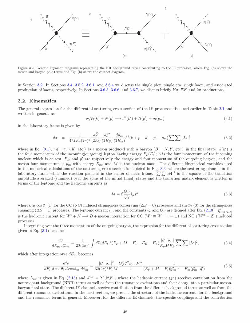
W

N

N(Y )

π(K)N

W

N(Y )

N(Y )

π(K) N

π(K)

N(Y )

(a) (b)

Figure 3.2: Generic Feynman diagrams representing the NR background terms contributing to the IE processes, where Fig. (a) shows themeson and baryon pole terms and Fig. (b) shows the contact diagram.

in Section 3.2. In Sections 3.4, 3.5.2, 3.6.1, and 3.6.4 we discuss the single pion, single eta, single kaon, and associatedproduction of kaons, respectively. In Sections 3.6.5, 3.6.6, and 3.6.7, we discuss briefly Y π, ΞK and 2π productions.

3.2. Kinematics

The general expression for the differential scattering cross section of the IE processes discussed earlier in Table-2.1 andwritten in general as

νl/νl(k) +N(p) −→ l∓(k′) +B(p′) +m(pm) (3.1)

in the laboratory frame is given by

dσ =1

4MEν(2π)5d~k′

(2El)

d~p ′

(2EB)

d~pm(2Em)

δ4(k + p− k′ − p′ − pm)∑∑

|M|2, (3.2)

where in Eq. (3.1), m(= π, η,K, etc.) is a meson produced with a baryon (B = N, Y , etc.) in the final state. k(k′) isthe four momentum of the incoming(outgoing) lepton having energy Eν(El); p is the four momentum of the incomingnucleon which is at rest, EB and p′ are respectively the energy and four momentum of the outgoing baryon, and themeson four momentum is pm with energy Em, and M is the nucleon mass. The different kinematical variables usedin the numerical calculations of the scattering cross section is depicted in Fig. 3.3, where the scattering plane is in thelaboratory frame while the reaction plane is in the center of mass frame.

∑∑ |M|2 is the square of the transitionamplitude averaged (summed) over the spins of the initial (final) states and the transition matrix element is written interms of the leptonic and the hadronic currents as

M = CGF√2lµj

µ, (3.3)

where C is cos θc (1) for the CC (NC) induced strangeness conserving (∆S = 0) processes and sin θC (0) for the strangenesschanging (∆S = 1) processes. The leptonic current lµ, and the constants θc and GF are defined after Eq. (2.10). jµCC(NC)

is the hadronic current for W i +N −→ B + meson interaction for CC (W i ≡ W± ; i = ±) and NC ((W 0 = Z0) inducedprocesses.

Integrating over the three momentum of the outgoing baryon, the expression for the differential scattering cross sectiongiven in Eq. (3.1) becomes

dσ

dEm dΩm=

1

32(2π)5

∫

dΩldEl δ(Eν +M − El − EB − Eπ)|~k′||~pm|EνMEB

∑∑

|M|2, (3.4)

which after integration over dEm becomes

d4σ

dEl d cos θl d cos θm dφm=

|~k′||~pm|232(2π)4EνM

G2F C2LµνJ

µν

4

1

(Eν +M − El)|~pm|2 − Em(~pm · ~q ), (3.5)

where Lµν is given in Eq. (2.15) and Jµν =∑

jµjν†, where the hadronic current (jµ) receives contribution from thenonresonant background (NRB) terms as well as from the resonance excitations and their decay into a particular meson-baryon final state. The different IE channels receive contribution from the different background terms as well as from thedifferent resonance excitations. In the next section, we present the structure of the hadronic currents for the backgroundand the resonance terms in general. Moreover, for the different IE channels, the specific couplings and the contribution

48

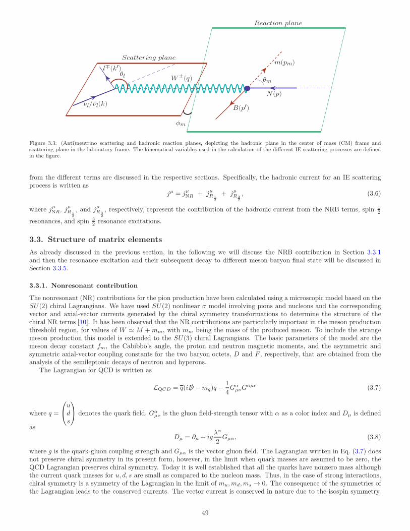
νl/νl(k)

θl W±(q)

φm

N (p)

m(pm)

B(p′)

l∓(k′)

θm

Scattering plane

Reaction plane

Figure 3.3: (Anti)neutrino scattering and hadronic reaction planes, depicting the hadronic plane in the center of mass (CM) frame andscattering plane in the laboratory frame. The kinematical variables used in the calculation of the different IE scattering processes are definedin the figure.

from the different terms are discussed in the respective sections. Specifically, the hadronic current for an IE scatteringprocess is written as

jµ = jµNR + jµR 12

+ jµR 32

, (3.6)

where jµNR, jµR 12

, and jµR 32

, respectively, represent the contribution of the hadronic current from the NRB terms, spin 12

resonances, and spin 32 resonance excitations.

3.3. Structure of matrix elements

As already discussed in the previous section, in the following we will discuss the NRB contribution in Section 3.3.1and then the resonance excitation and their subsequent decay to different meson-baryon final state will be discussed inSection 3.3.5.

3.3.1. Nonresonant contribution

The nonresonant (NR) contributions for the pion production have been calculated using a microscopic model based on theSU(2) chiral Lagrangians. We have used SU(2) nonlinear σ model involving pions and nucleons and the correspondingvector and axial-vector currents generated by the chiral symmetry transformations to determine the structure of thechiral NR terms [10]. It has been observed that the NR contributions are particularly important in the meson productionthreshold region, for values of W ≃ M +mm, with mm being the mass of the produced meson. To include the strangemeson production this model is extended to the SU(3) chiral Lagrangians. The basic parameters of the model are themeson decay constant fm, the Cabibbo’s angle, the proton and neutron magnetic moments, and the asymmetric andsymmetric axial-vector coupling constants for the two baryon octets, D and F , respectively, that are obtained from theanalysis of the semileptonic decays of neutron and hyperons.

The Lagrangian for QCD is written as

LQCD = q(i /D −mq)q −1

4Gα

µνGαµν (3.7)

where q =

uds

denotes the quark field, Gαµν is the gluon field-strength tensor with α as a color index and Dµ is defined

as

Dµ = ∂µ + igλα

2Gµα, (3.8)

where g is the quark-gluon coupling strength and Gµα is the vector gluon field. The Lagrangian written in Eq. (3.7) doesnot preserve chiral symmetry in its present form, however, in the limit when quark masses are assumed to be zero, theQCD Lagrangian preserves chiral symmetry. Today it is well established that all the quarks have nonzero mass althoughthe current quark masses for u, d, s are small as compared to the nucleon mass. Thus, in the case of strong interactions,chiral symmetry is a symmetry of the Lagrangian in the limit of mu,md,ms → 0. The consequence of the symmetries ofthe Lagrangian leads to the conserved currents. The vector current is conserved in nature due to the isospin symmetry.

49

Similarly the axial-vector current is conserved in the presence of the chiral symmetry. In case the chiral symmetry basedon SU(2) × SU(2) is broken spontaneously, it leads to the existence of massless Goldstone boson which are identifiedas the pion in the limit mu,md → 0 and as the octet of pseudoscalar mesons in the case of chiral symmetry based onSU(3)× SU(3) symmetry in the limit mu,md,ms → 0. The local gauge symmetry of QCD leads to the construction ofchiral effective theory of the Goldstone bosons as well as their interaction with the baryons.

In order to get the Lagrangian which describes the dynamics of these pseudoscalar mesons, we need continuous fieldswhich are described in terms of these Goldstone modes. The elements of SU(3) pseudoscalar meson fields are written interms of a unitary matrix [10]

U(Θ) = exp

(

−iΘkλk2

)

, (3.9)

where Θk; (k = 1− 8) are the real set of parameters and λk are the traceless, Hermitian 3× 3 Gell-Mann matrices.Each Goldstone boson corresponds to the x-dependent Cartesian component of the fields, φk(x), which in turn, is

expressed in terms of the physical fields as [10]:

Φ(x) =

8∑

k=1

φk(x)λk =

π0 + 1√3η

√2π+

√2K+

√2π− −π0 + 1√

3η√2K0

√2K− √

2K0 − 2√3η

. (3.10)

For the baryons, we follow the same procedure as we do for the mesons. However, unlike the pseudoscalar mesons wherethe fields are real, in the case of baryon fields, represented by a B matrix, each entry is a complex-field and the generalrepresentation is given by [10]:

B(x) =

8∑

k=1

1√2bk(x)λk =

1√2Σ0 + 1√

6Λ Σ+ p

Σ− − 1√2Σ0 + 1√

6Λ n

Ξ− Ξ0 − 2√6Λ

. (3.11)

After getting the representation of the pseudoscalar meson fields octet Φ(x) in Eq. (3.10) and baryon fields octet B(x)in Eq. (3.11), we now discuss the construction of the Lagrangian for meson-meson, baryon-meson interactions and theirinteraction with the external fields.

3.3.2. Meson - meson interaction

The lowest-order SU(3) chiral Lagrangian describing the pseudoscalar mesons in the presence of an external current isobtained as [232, 233]:

LM =f2π

4Tr[DµU(DµU)†]. (3.12)

The covariant derivatives DµU and DµU † appearing in Eq. (3.12) are expressed in terms of the partial derivatives as

DµU ≡ ∂µU − irµU + iUlµ, DµU † ≡ ∂µU † + iU †rµ − ilµU †, (3.13)

where U is the SU(3) unitary matrix given as

U(x) = exp

(

iΦ(x)

fπ

)

, (3.14)

where Φ(x) is given by Eq. (3.10). rµ and lµ, respectively, represent the right and left handed currents, defined in termsof the vector (vµ) and axial-vector (aµ) fields as

lµ =1

2(vµ − aµ), rµ =

1

2(vµ + aµ). (3.15)

The vector and axial-vector fields are different for the interaction of the different gauge bosons with the meson fields.In the case of electromagnetic interactions, the left and right handed currents are identical and are expressed as

lµ = rµ = −eQAµ, (3.16)

where e is the electric charge, Aµ represents the photon field and Q =

2/3 0 00 −1/3 00 0 −1/3

represents the charge of

the u, d, and s quarks. However, in the case of weak CC and NC induced processes, both vector and axial-vector fieldscontribute, thus, the left and right handed currents are expressed as

lµ = −g2(W+

µ T+ +W−µ T−), rµ = 0, (3.17)

50

where g = esin θW

, sin θW is the Weinberg angle, W±µ represents the W-boson field and T± is defined as

T+ =

0 Vud Vus0 0 00 0 0

, and T− =

0 0 0Vud 0 0Vus 0 0

, (3.18)

with Vud = cos θC and Vus = sin θC being the elements of the Cabibbo-Kobayashi-Maskawa matrix and θC being theCabibbo angle.

The left and right handed currents for NC induced processes are expressed as

lµ =

(

− g

cos θW+ e tan θW

)

Zµλ32, rµ = g tan θW sin θWZµ

λ32, (3.19)

where Zµ represents the Z-boson field and λ3 is the third component of the Gell-Mann matrices.

3.3.3. Baryon - meson interaction

To incorporate baryons in the theory, we have to take care of their masses which do not vanish in the chiral limit [234].However, if we take nucleons as massive matter fields which couples to external currents and the pseudoscalar mesons,we have to then expand the Lagrangian according to their increasing number of momenta. Here, we shall present in briefthe extension of the formalism to incorporate the heavy matter fields.

The lowest-order chiral Lagrangian for the baryon octet in the presence of an external current, may be written interms of the SU(3) matrix B as [232, 233],

LMB = Tr[

B(

i /D −M)

B]

− D

2Tr(

Bγµγ5uµ, B)

− F

2Tr(

Bγµγ5[uµ, B])

, (3.20)

where M denotes the mass of the baryon octet, D = 0.804 and F = 0.463 are the symmetric and antisymmetric axial-vector coupling constants for the baryon octet determined from the semileptonic decays of neutron and hyperons [235],the matrix B is given in Eq. (3.11) and the Lorentz vector uµ is given by [233]:

uµ = i[

u†(∂µ − irµ)u− u(∂µ − ilµ)u†]

. (3.21)

In the case of meson-baryon interactions, the unitary matrix for the pseudoscalar field is expressed as

u =√U ≡ exp

(

iΦ(x)

2fπ

)

, (3.22)

and the covariant derivative Dµ on the baryon fields B is given by

DµB = ∂µB + [Γµ, B], with Γµ =1

2

[

u†(∂µ − irµ)u + u(∂µ − ilµ)u†]

, (3.23)

which is known as the chiral connection.

3.3.4. Lagrangian for decuplet baryon-octet baryon-meson interaction

A systematic way of obtaining the relationships (SU(3) factors) between the weak vertices for all the allowed transitionsand that for the n −→ ∆+ is to use the lowest order Lagrangian that couples the decuplet baryons with the octet baryonsand mesons in the presence of an external current [236, 237] and that has been used in Refs. [137, 141, 147]. Its form is

LDBM = C(

ǫabc Tµ

ade(uµ)db B

ec + ǫabcBe

c (uµ)db T

µaed

)

, (3.24)

where B is given by Eq. (3.11), uµ is given in Eq. (3.21), and T µaed is the SU(3) representation of the Rarita-Schwinger

fields for the decuplet baryons. This representation is completely symmetric, which in the present notation is given by a3× 3× 3 array of matrices

Tabc =

∆++ 1√3∆+ 1√

3Σ∗+

1√3∆+ 1√

3∆0 1√

6Σ∗0

1√3Σ∗+ 1√

6Σ∗0 1√

3Ξ∗0

1√3∆+ 1√

3∆0 1√

6Σ∗0

1√3∆0 ∆− 1√

3Σ∗−

1√6Σ∗0 1√

3Σ∗− 1√

3Ξ∗−

1√3Σ∗+ 1√

6Σ∗0 1√

3Ξ∗0

1√6Σ∗0 1√

3Σ∗− 1√

3Ξ∗−

1√3Ξ∗0 1√

3Ξ∗− Ω−

. (3.25)

51

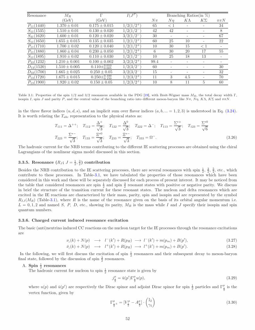
Resonance MR Γ I(JP ) Branching Ratios(in %)(GeV) (GeV) Nπ Nη KΛ KΣ ππN

P11(1440) 1.370± 0.01 0.175± 0.015 1/2(1/2+) 65 < 1 - - 34S11(1535) 1.510± 0.01 0.130± 0.020 1/2(1/2−) 42 42 - - 8S31(1620) 1.600± 0.01 0.120± 0.020 3/2(1/2−) 30 - - - 67S11(1650) 1.655± 0.015 0.135± 0.035 1/2(1/2+) 60 25 10 - 22P11(1710) 1.700± 0.02 0.120± 0.040 1/2(1/2+) 10 30 15 < 1 -P11(1880) 1.860± 0.04 0.230± 0.050 1/2(1/2+) 6 30 20 17 55S11(1895) 1.910± 0.02 0.110± 0.030 1/2(1/2−) 10 25 18 13 -P33(1232) 1.210± 0.001 0.100± 0.002 3/2(3/2+) 99.4 - - - -D13(1520) 1.510± 0.005 0.110±0.010

0.005 1/2(3/2−) 60 - - - 30D33(1700) 1.665± 0.025 0.250± 0.05 3/2(3/2−) 15 - - - 32P13(1720) 1.675± 0.015 0.250±0.100

0.150 1/2(3/2+) 11 3 4.5 - 70P13(1900) 1.920± 0.02 0.150± 0.05 1/2(3/2+) 10 8 11 5 60

Table 3.1: Properties of the spin 1/2 and 3/2 resonances available in the PDG [19], with Breit-Wigner mass MR, the total decay width Γ,isospin I, spin J and parity P , and the central value of the branching ratio into different meson-baryon like Nπ, Nη, KΛ, KΣ and ππN .

in the three flavor indices (u, d, s), and an implicit sum over flavor indices (a, b, ... = 1, 2, 3) is understood in Eq. (3.24).It is worth relating the Tabc representation to the physical states as:

T111 = ∆++; T112 =∆+

√3; T122 =

∆0

√3; T222 = ∆−; T113 =

Σ∗+√3; T123 =

Σ∗0√6

T223 =Σ∗−√3; T133 =

Ξ∗0√3; T233 =

Ξ∗−√3; T333 = Ω−. (3.26)

The hadronic current for the NRB terms contributing to the different IE scattering processes are obtained using the chiralLagrangians of the nonlinear sigma model discussed in this section.

3.3.5. Resonance (RJ ; J = 12 ,

32) contribution

Besides the NRB contribution to the IE scattering processes, there are several resonances with spin 12 , 3

2 , 52 , etc., which

contribute to these processes. In Table-3.1, we have tabulated the properties of those resonances which have beenconsidered in this work and these will be separately discussed for each process of present interest. It may be noticed fromthe table that considered resonances are spin 1

2 and spin 32 resonant states with positive or negative parity. We discuss

in brief the structure of the transition current for these resonant states. The nucleon and delta resonances which areexcited in the IE reactions are characterized by their mass, parity, spin and isospin and are represented by the symbolRIJ(MR) (Table-3.1), where R is the name of the resonance given on the basis of its orbital angular momentum i.e.L = 0, 1, 2 and named S, P, D, etc., showing its parity, MR is the mass while I and J specify their isospin and spinquantum numbers.

3.3.6. Charged current induced resonance excitation

The basic (anti)neutrino induced CC reactions on the nucleon target for the IE processes through the resonance excitationsare

νl(k) +N(p) −→ l−(k′) +R(pR) −→ l−(k′) +m(pm) +B(p′), (3.27)

νl(k) +N(p) −→ l+(k′) +R(pR) −→ l+(k′) +m(pm) +B(p′). (3.28)

In the following, we will first discuss the excitation of spin 12 resonances and their subsequent decay to meson-baryon

final state, followed by the discussion of spin 32 resonances.

A. Spin 12 resonances

The hadronic current for nucleon to spin 12 resonance state is given by

jµ12

= u(p′)Γµ12

u(p), (3.29)

where u(p) and u(p′) are respectively the Dirac spinor and adjoint Dirac spinor for spin 12 particles and Γµ

12

is the

vertex function, given by

Γµ12± = [V µ

12

−Aµ12

] ·(

I2

γ5

)

(3.30)

52

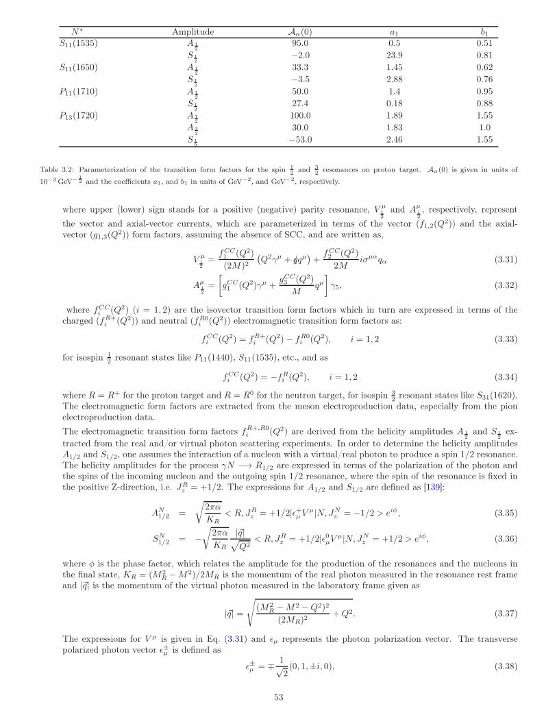
N∗ Amplitude Aα(0) a1 b1S11(1535) A 1

295.0 0.5 0.51

S 12

−2.0 23.9 0.81

S11(1650) A 12

33.3 1.45 0.62

S 12

−3.5 2.88 0.76

P11(1710) A 12

50.0 1.4 0.95

S 12

27.4 0.18 0.88

P13(1720) A 12

100.0 1.89 1.55

A 32

30.0 1.83 1.0

S 12

−53.0 2.46 1.55

Table 3.2: Parameterization of the transition form factors for the spin 12

and 32

resonances on proton target. Aα(0) is given in units of

10−3 GeV− 12 and the coefficients a1, and b1 in units of GeV−2, and GeV−2, respectively.

where upper (lower) sign stands for a positive (negative) parity resonance, V µ12

and Aµ12

, respectively, represent

the vector and axial-vector currents, which are parameterized in terms of the vector (f1,2(Q2)) and the axial-

vector (g1,3(Q2)) form factors, assuming the absence of SCC, and are written as,

V µ12

=fCC1 (Q2)

(2M)2(

Q2γµ + q/qµ)

+fCC2 (Q2)

2Miσµαqα (3.31)

Aµ12

=

[

gCC1 (Q2)γµ +

gCC3 (Q2)

Mqµ]

γ5, (3.32)

where fCCi (Q2) (i = 1, 2) are the isovector transition form factors which in turn are expressed in terms of the

charged (fR+i (Q2)) and neutral (fR0

i (Q2)) electromagnetic transition form factors as:

fCCi (Q2) = fR+

i (Q2)− fR0i (Q2), i = 1, 2 (3.33)

for isospin 12 resonant states like P11(1440), S11(1535), etc., and as

fCCi (Q2) = −fR

i (Q2), i = 1, 2 (3.34)

where R = R+ for the proton target and R = R0 for the neutron target, for isospin 32 resonant states like S31(1620).

The electromagnetic form factors are extracted from the meson electroproduction data, especially from the pionelectroproduction data.

The electromagnetic transition form factors fR+,R0i (Q2) are derived from the helicity amplitudes A 1

2and S 1

2ex-

tracted from the real and/or virtual photon scattering experiments. In order to determine the helicity amplitudesA1/2 and S1/2, one assumes the interaction of a nucleon with a virtual/real photon to produce a spin 1/2 resonance.The helicity amplitudes for the process γN −→ R1/2 are expressed in terms of the polarization of the photon andthe spins of the incoming nucleon and the outgoing spin 1/2 resonance, where the spin of the resonance is fixed inthe positive Z-direction, i.e. JR

z = +1/2. The expressions for A1/2 and S1/2 are defined as [139]:

AN1/2 =

√

2πα

KR< R, JR

z = +1/2|ǫ+µV µ|N, JNz = −1/2 > eiφ, (3.35)

SN1/2 = −

√

2πα

KR

|~q|√

Q2< R, JR

z = +1/2|ǫ0µV µ|N, JNz = +1/2 > eiφ, (3.36)

where φ is the phase factor, which relates the amplitude for the production of the resonances and the nucleons inthe final state, KR = (M2

R −M2)/2MR is the momentum of the real photon measured in the resonance rest frameand |~q| is the momentum of the virtual photon measured in the laboratory frame given as

|~q| =√

(M2R −M2 −Q2)2

(2MR)2+Q2. (3.37)

The expressions for V µ is given in Eq. (3.31) and ǫµ represents the photon polarization vector. The transversepolarized photon vector ǫ±µ is defined as

ǫ±µ = ∓ 1√2(0, 1,±i, 0), (3.38)

53

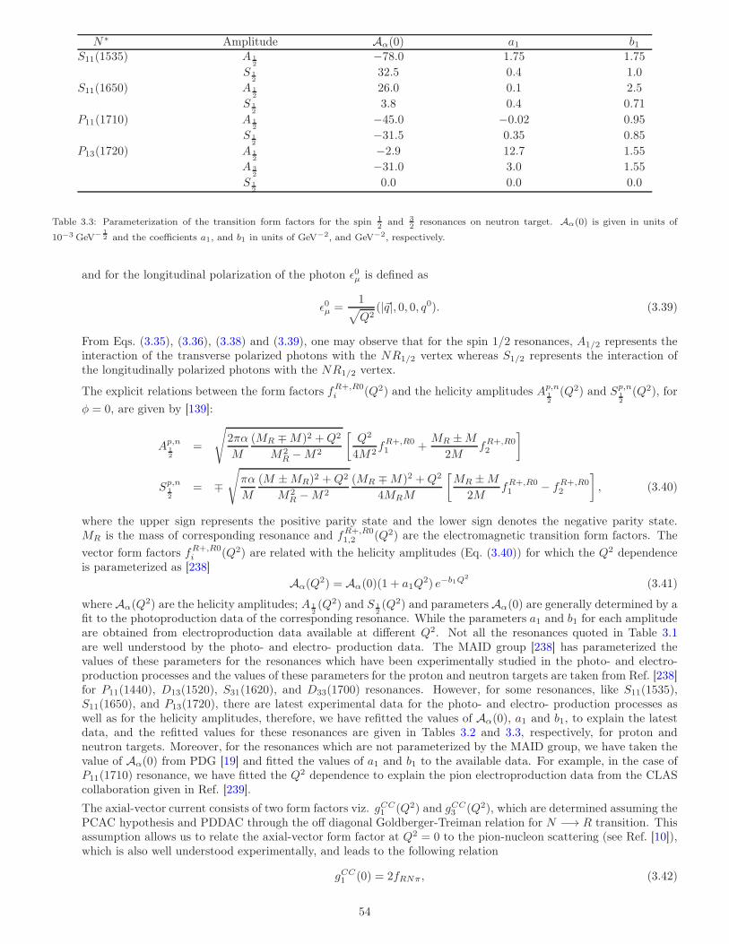
N∗ Amplitude Aα(0) a1 b1S11(1535) A 1

2−78.0 1.75 1.75

S 12

32.5 0.4 1.0

S11(1650) A 12

26.0 0.1 2.5

S 12

3.8 0.4 0.71

P11(1710) A 12

−45.0 −0.02 0.95

S 12

−31.5 0.35 0.85

P13(1720) A 12

−2.9 12.7 1.55

A 32

−31.0 3.0 1.55

S 12

0.0 0.0 0.0

Table 3.3: Parameterization of the transition form factors for the spin 12

and 32

resonances on neutron target. Aα(0) is given in units of

10−3 GeV− 12 and the coefficients a1, and b1 in units of GeV−2, and GeV−2, respectively.

and for the longitudinal polarization of the photon ǫ0µ is defined as

ǫ0µ =1

√

Q2(|~q|, 0, 0, q0). (3.39)

From Eqs. (3.35), (3.36), (3.38) and (3.39), one may observe that for the spin 1/2 resonances, A1/2 represents theinteraction of the transverse polarized photons with the NR1/2 vertex whereas S1/2 represents the interaction ofthe longitudinally polarized photons with the NR1/2 vertex.

The explicit relations between the form factors fR+,R0i (Q2) and the helicity amplitudes Ap,n

12

(Q2) and Sp,n12

(Q2), for

φ = 0, are given by [139]:

Ap,n12

=

√

2πα

M

(MR ∓M)2 +Q2

M2R −M2

[

Q2

4M2fR+,R01 +

MR ±M2M

fR+,R02

]

Sp,n12

= ∓√

πα

M

(M ±MR)2 +Q2

M2R −M2

(MR ∓M)2 +Q2

4MRM

[

MR ±M2M

fR+,R01 − fR+,R0

2

]

, (3.40)

where the upper sign represents the positive parity state and the lower sign denotes the negative parity state.MR is the mass of corresponding resonance and fR+,R0

1,2 (Q2) are the electromagnetic transition form factors. The

vector form factors fR+,R0i (Q2) are related with the helicity amplitudes (Eq. (3.40)) for which the Q2 dependence

is parameterized as [238]

Aα(Q2) = Aα(0)(1 + a1Q

2) e−b1Q2

(3.41)

where Aα(Q2) are the helicity amplitudes; A 1

2(Q2) and S 1

2(Q2) and parameters Aα(0) are generally determined by a

fit to the photoproduction data of the corresponding resonance. While the parameters a1 and b1 for each amplitudeare obtained from electroproduction data available at different Q2. Not all the resonances quoted in Table 3.1are well understood by the photo- and electro- production data. The MAID group [238] has parameterized thevalues of these parameters for the resonances which have been experimentally studied in the photo- and electro-production processes and the values of these parameters for the proton and neutron targets are taken from Ref. [238]for P11(1440), D13(1520), S31(1620), and D33(1700) resonances. However, for some resonances, like S11(1535),S11(1650), and P13(1720), there are latest experimental data for the photo- and electro- production processes aswell as for the helicity amplitudes, therefore, we have refitted the values of Aα(0), a1 and b1, to explain the latestdata, and the refitted values for these resonances are given in Tables 3.2 and 3.3, respectively, for proton andneutron targets. Moreover, for the resonances which are not parameterized by the MAID group, we have taken thevalue of Aα(0) from PDG [19] and fitted the values of a1 and b1 to the available data. For example, in the case ofP11(1710) resonance, we have fitted the Q2 dependence to explain the pion electroproduction data from the CLAScollaboration given in Ref. [239].

The axial-vector current consists of two form factors viz. gCC1 (Q2) and gCC

3 (Q2), which are determined assuming thePCAC hypothesis and PDDAC through the off diagonal Goldberger-Treiman relation for N −→ R transition. Thisassumption allows us to relate the axial-vector form factor at Q2 = 0 to the pion-nucleon scattering (see Ref. [10]),which is also well understood experimentally, and leads to the following relation

gCC1 (0) = 2fRNπ, (3.42)

54

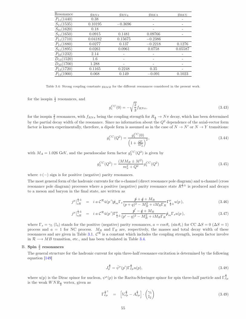
Resonance gRNπ gRNη gRKΛ gRKΣ

P11(1440) 0.38 - - -S11(1535) 0.10195 −0.3696 - -S31(1620) 0.18 - - -S11(1650) 0.0915 0.1481 0.09766 -P11(1710) 0.04182 0.15675 −0.2386P11(1880) 0.0277 0.137 −0.2218 0.1276S11(1895) 0.0261 0.0961 0.0758 0.05587P33(1232) 2.14 - - -D13(1520) 1.6 - - -D33(1700) 1.288 - - -P13(1720) 0.1165 0.2248 0.35 -P13(1900) 0.068 0.149 −0.091 0.1023

Table 3.4: Strong coupling constants gRMB for the different resonances considered in the present work.

for the isospin 12 resonances, and

gCC1 (0) = −

√

2

3fRNπ, (3.43)

for the isospin 32 resonances, with fRNπ being the coupling strength for R 1

2→ Nπ decay, which has been determined

by the partial decay width of the resonance. Since no information about the Q2 dependence of the axial-vector formfactor is known experimentally, therefore, a dipole form is assumed as in the case of N → N ′ or N → Y transitions:

gCC1 (Q2) =

gCC1 (0)

(

1 + Q2

M2A

)2 , (3.44)

with MA = 1.026 GeV, and the pseudoscalar form factor gCC3 (Q2) is given by

gCC3 (Q2) =

(MMR ±M2)

m2π +Q2

gCC1 (Q2) (3.45)

where +(−) sign is for positive (negative) parity resonances.

The most general form of the hadronic currents for the s-channel (direct resonance pole diagram) and u-channel (cross

resonance pole diagram) processes where a positive (negative) parity resonance state R12± is produced and decays

to a meson and baryon in the final state, are written as

jµ∣

∣

12±sR

= i a CRu(p ′)p/mΓsp/ + q/+MR

(p+ q)2 −M2R + iMRΓR

Γµ12±u(p ), (3.46)

jµ∣

∣

12±uR

= i a CRu(p ′)Γµ12±

p/′ − q/+MR

(p′ − q)2 −M2R + iMRΓR

p/mΓsu(p ), (3.47)

where Γs = γ5 (I4) stands for the positive (negative) parity resonances, a = cos θc (sin θc) for CC ∆S = 0 (∆S = 1)process and a = 1 for NC process. MR and ΓR are, respectively, the masses and total decay width of theseresonances and are given in Table 3.1. CR is a constant which includes the coupling strength, isospin factor involvein R −→MB transition, etc., and has been tabulated in Table 3.4.

B. Spin 32 resonances

The general structure for the hadronic current for spin three-half resonance excitation is determined by the followingequation [149]

J32µ = ψν(p′)Γ

32νµu(p), (3.48)

where u(p) is the Dirac spinor for nucleon, ψµ(p) is the Rarita-Schwinger spinor for spin three-half particle and Γ32νµ

is the weak WNR 32

vertex, given as

Γ32±

νµ =[

V32νµ −A

32νµ

]

·(

γ5I2

)

(3.49)

55

where upper (lower) sign stands for a positive (negative) parity resonance, and V 32(A 3

2) is the vector (axial-vector)

current for spin three-half resonances. The vector and the axial-vector part of the currents are given by

V32νµ =

[

CV3

M(gµνq/ − qνγµ) +

CV4

M2(gµνq · p′ − qνp′µ) +

CV5

M2(gµνq · p− qνpµ) + gµνC

V6

]

(3.50)

A32νµ = −

[

CA3

M(gµνq/ − qνγµ) +

CA4

M2(gµνq · p′ − qνp′µ) + CA

5 gµν +CA

6

M2qνqµ

]

γ5 (3.51)

where CVi and CA

i are the vector and axial-vector CC transition form factors which are functions of Q2. The CVChypothesis leads to CV

6 (Q2) = 0.

The isovector CVi ; (i = 3, 4, 5) form factors for the resonance which have J = 3

2 , I = 12 , like D13(1520), P13(1720),

etc., are written in terms of the electromagnetic charged (CR+i (Q2)) and neutral (CR0

i (Q2)) transition form factorsthrough a simple relation [240] as

CVi = CR+

i − CR0i ; i = 3, 4, 5 , (3.52)

while for the resonance with J = 32 and I = 3

2 like P33(1232), D33(1700), etc., the isovector form factors CVi ; (i =

3, 4, 5) are expressed asCV

i = −CNi ; i = 3, 4, 5 , (3.53)

with N = R0 (R+) stands for the neutral (charged) electromagnetic form factor.

In the case of spin 3/2 resonances, along with i.e. JRz = +1/2, JR

z = +3/2 also contributes in the positive Z-direction. Again it is our choice to take JR

z in the positive Z-direction, one may obtain the expressions for thehelicity amplitudes by fixing JR

z in the negative Z-direction. The expressions for A1/2 and S1/2 in terms of thematrix element of V µ are given in Eqs. (3.35) and (3.36) with V µ defined in Eq. (3.50). The expression for A3/2 isgiven below:

AN3/2 =

√

2πα

KR< R, JR

z = +3/2|ǫ+µV µ|N, JNz = +1/2 > eiφ. (3.54)

The relations between the vector form factors CR+,R0i (Q2) and helicity amplitudes are given as [241]:

Ap,n32

=

√

πα

M

(MR ∓M)2 +Q2

M2R −M2

[

CR+,R03

M(M ±MR)±

CR+,R04

M2

M2R −M2 −Q2

2

± CR+,R05

M2

M2R −M2 +Q2

2

]

(3.55)

Ap,n12

=

√

πα

3M

(MR ∓M)2 +Q2

M2R −M2

[

CR+,R03

M

M2 +MMR +Q2

MR− CR+,R0

4

M2

M2R −M2 −Q2

2

− CR+,R05

M2

M2R −M2 +Q2

2

]

(3.56)

Sp,n12

= ±√

πα

6M

(MR ∓M)2 +Q2

M2R −M2

√

Q4 + 2Q2(M2R +M2) + (M2

R −M2)2

M2R

×[

CR+,R03

MMR +

CR+,R04

M2M2

R +CR+,R0

5

M2

M2R +M2 +Q2

2

]

, (3.57)

where upper (lower) signs stand for the positive (negative) parity resonances, A 32(Q2), A 1

2(Q2), and S 1

2(Q2) are the

amplitudes corresponding to the transverse and longitudinal polarizations, respectively and are parameterized atdifferent Q2 using Eq. (3.41). Once the parameters a1 and b1 are fixed for A 3

2(Q2), A 1

2(Q2), and S 1

2(Q2) amplitudes,

one gets the form factors Cp,ni (Q2).

For the ∆(1232) resonance, the three vector form factors CVi , i = 3, 4, 5 are given in terms of the isovector electro-

magnetic form factors for p −→ ∆+ transition and the parameterization of which are taken from the Ref. [242],

CV3 (Q2) =

2.13

(1 +Q2/M2V )

2× 1

1 + Q2

4M2V

, CV4 (Q2) =

−1.51(1 +Q2/M2

V )2× 1

1 + Q2

4M2V

,

CV5 (Q2) =

0.48

(1 +Q2/M2V )

2× 1

1 + Q2

0.776M2V

(3.58)

56

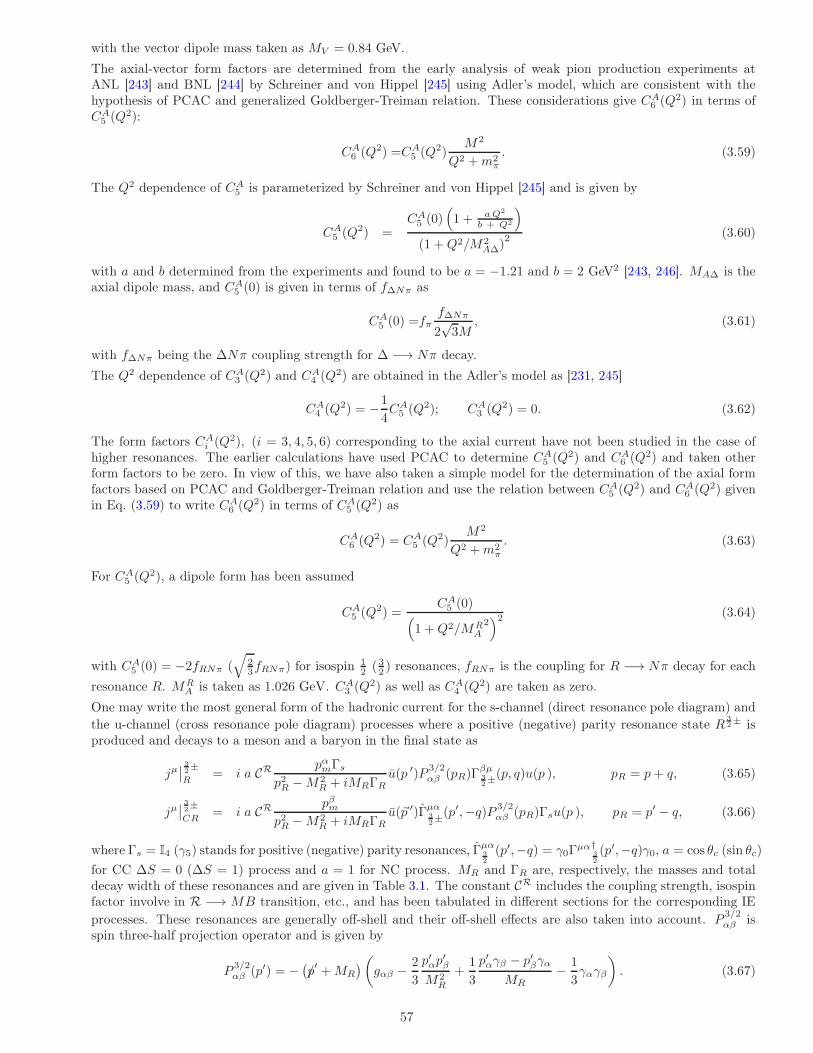
with the vector dipole mass taken as MV = 0.84 GeV.

The axial-vector form factors are determined from the early analysis of weak pion production experiments atANL [243] and BNL [244] by Schreiner and von Hippel [245] using Adler’s model, which are consistent with thehypothesis of PCAC and generalized Goldberger-Treiman relation. These considerations give CA

6 (Q2) in terms ofCA

5 (Q2):

CA6 (Q2) =CA

5 (Q2)M2

Q2 +m2π

. (3.59)

The Q2 dependence of CA5 is parameterized by Schreiner and von Hippel [245] and is given by

CA5 (Q2) =

CA5 (0)

(

1 + aQ2

b + Q2

)

(1 +Q2/M2A∆)

2 (3.60)

with a and b determined from the experiments and found to be a = −1.21 and b = 2 GeV2 [243, 246]. MA∆ is theaxial dipole mass, and CA

5 (0) is given in terms of f∆Nπ as

CA5 (0) =fπ

f∆Nπ

2√3M

, (3.61)

with f∆Nπ being the ∆Nπ coupling strength for ∆ −→ Nπ decay.

The Q2 dependence of CA3 (Q2) and CA

4 (Q2) are obtained in the Adler’s model as [231, 245]

CA4 (Q2) = −1

4CA

5 (Q2); CA3 (Q2) = 0. (3.62)

The form factors CAi (Q2), (i = 3, 4, 5, 6) corresponding to the axial current have not been studied in the case of

higher resonances. The earlier calculations have used PCAC to determine CA5 (Q2) and CA

6 (Q2) and taken otherform factors to be zero. In view of this, we have also taken a simple model for the determination of the axial formfactors based on PCAC and Goldberger-Treiman relation and use the relation between CA

5 (Q2) and CA6 (Q2) given

in Eq. (3.59) to write CA6 (Q2) in terms of CA

5 (Q2) as

CA6 (Q2) = CA

5 (Q2)M2

Q2 +m2π

. (3.63)

For CA5 (Q2), a dipole form has been assumed

CA5 (Q2) =

CA5 (0)

(

1 +Q2/MR

A2)2 (3.64)

with CA5 (0) = −2fRNπ (

√

23fRNπ) for isospin 1

2 (32 ) resonances, fRNπ is the coupling for R −→ Nπ decay for each

resonance R. MR

A is taken as 1.026 GeV. CA3 (Q2) as well as CA

4 (Q2) are taken as zero.

One may write the most general form of the hadronic current for the s-channel (direct resonance pole diagram) and

the u-channel (cross resonance pole diagram) processes where a positive (negative) parity resonance state R32± is

produced and decays to a meson and a baryon in the final state as

jµ∣

∣

32±R

= i a CR pαmΓs

p2R −M2R + iMRΓR

u(p ′)P3/2αβ (pR)Γ

βµ32±

(p, q)u(p ), pR = p+ q, (3.65)

jµ∣

∣

32±CR

= i a CR pβmp2R −M2

R + iMRΓRu(~p ′)Γµα

32±

(p′,−q)P 3/2αβ (pR)Γsu(p ), pR = p′ − q, (3.66)

where Γs = I4 (γ5) stands for positive (negative) parity resonances, Γµα32

(p′,−q) = γ0Γµα†

32

(p′,−q)γ0, a = cos θc (sin θc)

for CC ∆S = 0 (∆S = 1) process and a = 1 for NC process. MR and ΓR are, respectively, the masses and totaldecay width of these resonances and are given in Table 3.1. The constant CR includes the coupling strength, isospinfactor involve in R −→ MB transition, etc., and has been tabulated in different sections for the corresponding IE

processes. These resonances are generally off-shell and their off-shell effects are also taken into account. P3/2αβ is

spin three-half projection operator and is given by

P3/2αβ (p′) = −

(

p/′ +MR

)

(

gαβ −2

3

p′αp′β

M2R

+1

3

p′αγβ − p′βγαMR

− 1

3γαγβ

)

. (3.67)

57

The structure of the matrix element for the hadronic current is given in Eqs. (3.65)–(3.66) for positive and negativeparity resonances, respectively, and the weak vertex for positive and negative parity states are given in Eq. (3.49).The vector and axial-vector pieces are written in Eqs. (3.50) and (3.51), respectively, with corresponding formfactors, CV

i and CAi , defined for each resonances.

3.3.7. Neutral current (anti)neutrino induced resonance excitation processes

In this section, we present in brief the structure of resonance terms that may contribute to the hadronic current of(anti)neutrino induced NC processes. The basic NC (anti)neutrino induced reactions for meson production throughresonance excitations are the following:

νl(k) +N(p) −→ νl(k

′) +R(pR) −→ νl(k′) +B(p′) +m(pm), (3.68)

νl(k) +N(p) −→ νl(k

′) +R(pR) −→ νl(k′) +B(p′) +m(pm), (3.69)

where R stands for the resonances (R) which contribute to the meson production. We will discuss separately thecontribution of spin 1

2 and 32 resonances to NC induced single meson production.

A. Spin 12 resonances

For NC process producing a spin 12 resonance in the intermediate state, the hadronic current is given by Eq. (3.29).

Γµ12

is the vertex function which for positive and negative parity states is given in Eq. (3.30). The vector and axial-

vector parts of the current are written in terms of vector and axial-vector form factors and have the same form asgiven in Eqs. (3.31) and (3.32), but with a modified form factor and a different expression for charged (fR+

i ) and

neutral (fR0i ) resonance states with the replacement of fCC

1,2 by fR+,R01,2 , corresponding to isospin 1

2 resonance.

In the case of isospin 12 resonances, the explicit expressions for the vector and axial-vector form factors are written

as

fpi (Q

2) =

(

1

2− 2 sin2 θW

)

fR+i (Q2)− 1

2fR0i (Q2), gp1(Q

2) =1

2gCC1 (Q2) (3.70)

for the positive charged state and

fni (Q

2) =

(

1

2− 2 sin2 θW

)

fR0i (Q2)− 1

2fR+i (Q2), gn1 (Q

2) = −1

2gCC1 (Q2) (3.71)

for the neutral state. While for the case of isospin 32 resonances, these form factors fp

i and fni are given as:

fpi (Q

2) = (1 − 2 sin2 θW )fR+i (Q2), gp1(Q

2) = −gCC1 (Q2) (3.72)

for the positive charged state and

fni (Q

2) = (1 − 2 sin2 θW )FR0i (Q2), gn1 (Q

2) = −gCC1 (Q2), (3.73)

for the neutral state.

B. Spin 32 resonances

The general structure for the hadronic current J32µ for NC induced spin 3

2 resonance in the intermediate state is

given by Eq. (3.48), for which Γ32+,−νµ is given by Eq. (3.49) for positive and negative parity states. The vector

and axial-vector parts of the current are given by Eqs. (3.50) and (3.51) with the corresponding NC form factors(CV

i ) (i = 3, 4, 5) and (CAi ) (i = 4, 5, 6) which in the SM are given in terms of CV

i and CAi .

The NC form factors CVi and CA

i (i = 3, 4, 5) for the case of isospin 12 resonances, are given by:

(CVi )

for p−→ (1

2− 2 sin2 θW )Cp

i −1

2Cn

i , (CVi )

for n−→ (1

2− 2 sin2 θW )Cn

i −1

2Cp

i , (CAi )

for p,n−→ ±1

2CA

i , (3.74)

while for the isospin 32 resonances, NC form factors are given as:

(CVi )

for p−→ (1− 2 sin2 θW )Cpi , (CV

i )for n−→ (1− 2 sin2 θW )Cn

i , (CAi )

for p,n−→ −CAi . (3.75)

58

3.3.8. Strong couplings of the resonances

Due to the lack of experimental data there is large uncertainty associated with RMB coupling at the R → MB vertex.We have fixed RMB coupling using the data of branching ratio and decay width of these resonances from PDG [19]and use the expression for the decay rate which is obtained by writing the most general form of RMB Lagrangian givenby [10]:

LR 12MB =

fR 12MB

fmΨR 1

2

Γµ12

∂µφiTiΨ (3.76)

LR 32MB =

fR 32MB

fmΨR 3

2

Γµ32

∂µφiTi Ψ (3.77)

where fm is the meson decay constant, which in the case of pion production becomes fm = fπ = 92.4 MeV [19] and foreta and kaon production becomes fm = fη = fK = 105 MeV [247]. fR 1

2MB and fR 32MB are, respectively, the RMB

coupling strength for spin 12 and 3

2 resonances. Ψ is the nucleon field and ΨR 12

and ΨR 32

are the fields associated with the

resonances of spin 12 and spin 3

2 , respectively. φi are the mesonic field and Ti are the isospin operator which is T = ~τ forisospin 1

2 states and T = T † for isospin 32 states (~τ and T † are the isospin operator for doublet and quartet, respectively).

The interaction vertex Γµ12

is γµγ5 (γµ) for spin 12 resonances with positive (negative) parity. Similarly, the interaction

vertex Γµ32

, for spin 32 resonances for positive (negative) parity state, are I4 (γ5). Using the above Lagrangian one may

obtain the expression for the decay width in the resonance rest frame as

ΓR 12−→MB =

C4π

(

fR 12MB

fm

)2

(MR ±MB)2 EN ∓MB

MR|~qcm| (3.78)

ΓR 32−→MB =

C12π

(

fR 32MB

fm

)2EN ±MB

MR|~qcm|3, (3.79)

where the upper(lower) sign represents the positive(negative) parity resonance state. The parameter C is obtained fromthe isospin analysis and found out to be 3 for isospin 1

2 state and 1 for isospin 32 states. |~qcm| is the outgoing pion

momentum measured from resonance rest frame and EN is the nucleon energy, which are given by,

|~qcm| =√

(W 2 −m2m −M2

B)2 − 4m2

MM2B

2MR, EN =

W 2 +M2B −m2

m

2MR, (3.80)

where W is the CM energy carried by the resonance.In view of the above, we fix N∆π coupling(fπN∆) by comparing ∆→ Nπ decay width evaluated in the rest frame of

∆ resonance,

Γ∆(s) =1

6π

(

fπN∆

mπ

)2M√s

[

λ12 (s,m2

π,M2)

2√s

]3

Θ(√s−M −mπ), s = p2∆ (3.81)

where λ(x, y, z) = x2 + y2 + z2 − 2xy − 2xz − 2yz is Källen function. To get the offshell effect of ∆(1232) resonance wehave taken momentum dependent width.

3.4. Single pion production

Historically, the weak pion production induced by (anti)neutrinos has been studied for a long time starting from 1962 [248,249, 250, 251] in the energy region of (anti)neutrinos relevant for the early experiments done at CERN, ANL and BNL.These early calculations used various approaches based on the

(i) dynamical models with dispersion theory,

(ii) quark models with higher symmetry like SU(6), and

(iii) phenomenological Lagrangians for describing the interaction of mesons with nucleons and excitation of higherresonances.

These calculations have been comprehensively summarized by Adler [231], Llewellyn Smith [149] and Schreiner and vonHippel [245].

In the low energy region corresponding to the threshold production of pions various theoretical models motivatedby the chiral symmetry were used to study these processes. For example, the low energy theorems (LET) based onPCAC and/or current algebra (CA) as well as the effective Lagrangians incorporating the chiral symmetry which were

59

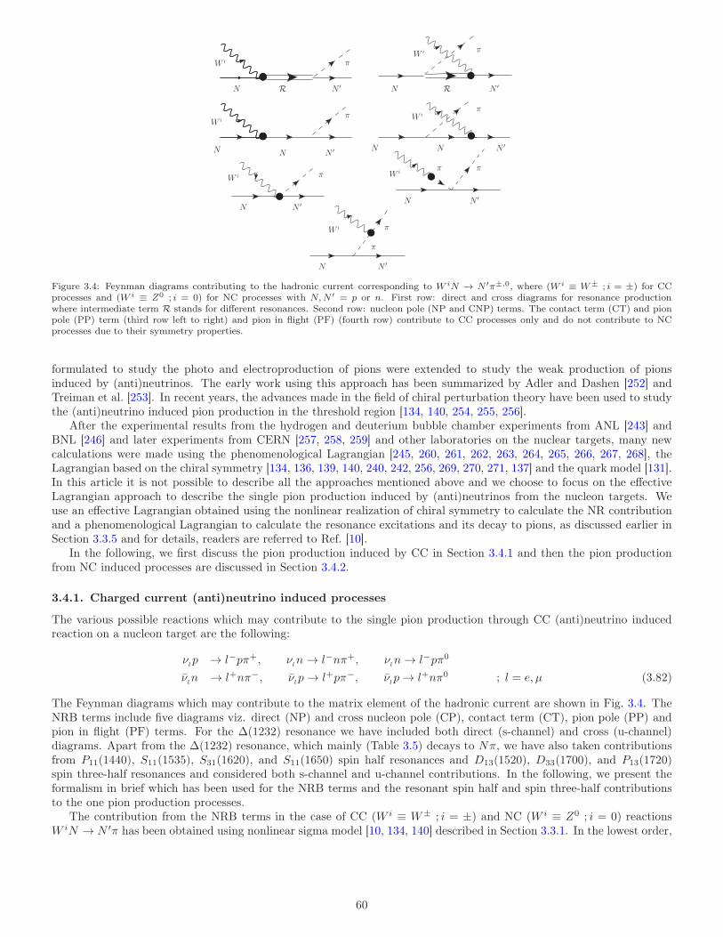
N R N ′

π

N

NN

N

N

W i

W iW i

W i

W iW i

R

N N ′

ππ

N ′N

π

π

π

π

W i

N ′

NN ′

π

π

N ′

N ′

Figure 3.4: Feynman diagrams contributing to the hadronic current corresponding to W iN → N ′π±,0, where (W i ≡ W± ; i = ±) for CCprocesses and (W i ≡ Z0 ; i = 0) for NC processes with N,N ′ = p or n. First row: direct and cross diagrams for resonance productionwhere intermediate term R stands for different resonances. Second row: nucleon pole (NP and CNP) terms. The contact term (CT) and pionpole (PP) term (third row left to right) and pion in flight (PF) (fourth row) contribute to CC processes only and do not contribute to NCprocesses due to their symmetry properties.

formulated to study the photo and electroproduction of pions were extended to study the weak production of pionsinduced by (anti)neutrinos. The early work using this approach has been summarized by Adler and Dashen [252] andTreiman et al. [253]. In recent years, the advances made in the field of chiral perturbation theory have been used to studythe (anti)neutrino induced pion production in the threshold region [134, 140, 254, 255, 256].

After the experimental results from the hydrogen and deuterium bubble chamber experiments from ANL [243] andBNL [246] and later experiments from CERN [257, 258, 259] and other laboratories on the nuclear targets, many newcalculations were made using the phenomenological Lagrangian [245, 260, 261, 262, 263, 264, 265, 266, 267, 268], theLagrangian based on the chiral symmetry [134, 136, 139, 140, 240, 242, 256, 269, 270, 271, 137] and the quark model [131].In this article it is not possible to describe all the approaches mentioned above and we choose to focus on the effectiveLagrangian approach to describe the single pion production induced by (anti)neutrinos from the nucleon targets. Weuse an effective Lagrangian obtained using the nonlinear realization of chiral symmetry to calculate the NR contributionand a phenomenological Lagrangian to calculate the resonance excitations and its decay to pions, as discussed earlier inSection 3.3.5 and for details, readers are referred to Ref. [10].

In the following, we first discuss the pion production induced by CC in Section 3.4.1 and then the pion productionfrom NC induced processes are discussed in Section 3.4.2.

3.4.1. Charged current (anti)neutrino induced processes

The various possible reactions which may contribute to the single pion production through CC (anti)neutrino inducedreaction on a nucleon target are the following:

νlp → l−pπ+, ν

ln→ l−nπ+, ν

ln→ l−pπ0

νln → l+nπ−, ν

lp→ l+pπ−, ν

lp→ l+nπ0 ; l = e, µ (3.82)

The Feynman diagrams which may contribute to the matrix element of the hadronic current are shown in Fig. 3.4. TheNRB terms include five diagrams viz. direct (NP) and cross nucleon pole (CP), contact term (CT), pion pole (PP) andpion in flight (PF) terms. For the ∆(1232) resonance we have included both direct (s-channel) and cross (u-channel)diagrams. Apart from the ∆(1232) resonance, which mainly (Table 3.5) decays to Nπ, we have also taken contributionsfrom P11(1440), S11(1535), S31(1620), and S11(1650) spin half resonances and D13(1520), D33(1700), and P13(1720)spin three-half resonances and considered both s-channel and u-channel contributions. In the following, we present theformalism in brief which has been used for the NRB terms and the resonant spin half and spin three-half contributionsto the one pion production processes.

The contribution from the NRB terms in the case of CC (W i ≡ W± ; i = ±) and NC (W i ≡ Z0 ; i = 0) reactionsW iN → N ′π has been obtained using nonlinear sigma model [10, 134, 140] described in Section 3.3.1. In the lowest order,

60

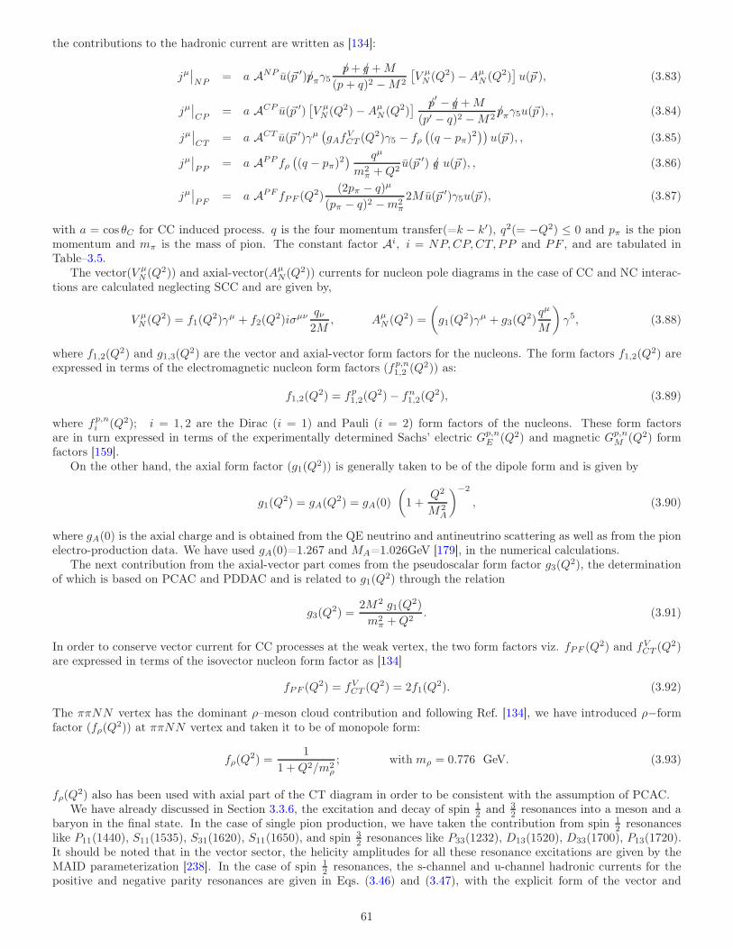
the contributions to the hadronic current are written as [134]:

jµ∣

∣

NP= a ANP u(~p ′)p/πγ5

p/+ q/ +M

(p+ q)2 −M2

[

V µN (Q2)−Aµ

N (Q2)]

u(~p ), (3.83)

jµ∣

∣

CP= a ACP u(~p ′)

[

V µN (Q2)−Aµ

N (Q2)] p/′ − q/ +M

(p′ − q)2 −M2p/πγ5u(~p ), , (3.84)

jµ∣

∣

CT= a ACT u(~p ′)γµ

(

gAfVCT (Q

2)γ5 − fρ(

(q − pπ)2))

u(~p ), , (3.85)

jµ∣

∣

PP= a APP fρ

(

(q − pπ)2) qµ

m2π +Q2

u(~p ′) q/ u(~p ), , (3.86)

jµ∣

∣

PF= a APF fPF (Q

2)(2pπ − q)µ

(pπ − q)2 −m2π

2Mu(~p ′)γ5u(~p ), (3.87)

with a = cos θC for CC induced process. q is the four momentum transfer(=k − k′), q2(= −Q2) ≤ 0 and pπ is the pionmomentum and mπ is the mass of pion. The constant factor Ai, i = NP,CP,CT, PP and PF , and are tabulated inTable–3.5.

The vector(V µN(Q2)) and axial-vector(Aµ

N(Q2)) currents for nucleon pole diagrams in the case of CC and NC interac-tions are calculated neglecting SCC and are given by,

V µN (Q2) = f1(Q

2)γµ + f2(Q2)iσµν qν

2M, Aµ

N (Q2) =

(

g1(Q2)γµ + g3(Q

2)qµ

M

)

γ5, (3.88)

where f1,2(Q2) and g1,3(Q

2) are the vector and axial-vector form factors for the nucleons. The form factors f1,2(Q2) are

expressed in terms of the electromagnetic nucleon form factors (fp,n1,2 (Q

2)) as:

f1,2(Q2) = fp

1,2(Q2)− fn

1,2(Q2), (3.89)

where fp,ni (Q2); i = 1, 2 are the Dirac (i = 1) and Pauli (i = 2) form factors of the nucleons. These form factors

are in turn expressed in terms of the experimentally determined Sachs’ electric Gp,nE (Q2) and magnetic Gp,n

M (Q2) formfactors [159].

On the other hand, the axial form factor (g1(Q2)) is generally taken to be of the dipole form and is given by

g1(Q2) = gA(Q

2) = gA(0)

(

1 +Q2

M2A

)−2

, (3.90)

where gA(0) is the axial charge and is obtained from the QE neutrino and antineutrino scattering as well as from the pionelectro-production data. We have used gA(0)=1.267 and MA=1.026GeV [179], in the numerical calculations.

The next contribution from the axial-vector part comes from the pseudoscalar form factor g3(Q2), the determination

of which is based on PCAC and PDDAC and is related to g1(Q2) through the relation

g3(Q2) =

2M2 g1(Q2)

m2π +Q2

. (3.91)

In order to conserve vector current for CC processes at the weak vertex, the two form factors viz. fPF (Q2) and fV

CT (Q2)

are expressed in terms of the isovector nucleon form factor as [134]

fPF (Q2) = fV

CT (Q2) = 2f1(Q

2). (3.92)

The ππNN vertex has the dominant ρ–meson cloud contribution and following Ref. [134], we have introduced ρ−formfactor (fρ(Q

2)) at ππNN vertex and taken it to be of monopole form:

fρ(Q2) =

1

1 +Q2/m2ρ

; with mρ = 0.776 GeV. (3.93)

fρ(Q2) also has been used with axial part of the CT diagram in order to be consistent with the assumption of PCAC.

We have already discussed in Section 3.3.6, the excitation and decay of spin 12 and 3

2 resonances into a meson and abaryon in the final state. In the case of single pion production, we have taken the contribution from spin 1

2 resonanceslike P11(1440), S11(1535), S31(1620), S11(1650), and spin 3

2 resonances like P33(1232), D13(1520), D33(1700), P13(1720).It should be noted that in the vector sector, the helicity amplitudes for all these resonance excitations are given by theMAID parameterization [238]. In the case of spin 1

2 resonances, the s-channel and u-channel hadronic currents for thepositive and negative parity resonances are given in Eqs. (3.46) and (3.47), with the explicit form of the vector and

61

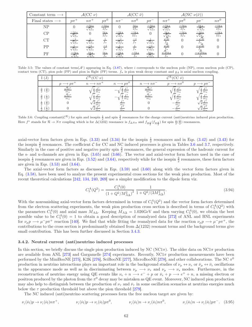
Constant term −→ A(CC ν) A(CC ν) A(NC ν(ν))

Final states −→ pπ+ nπ+ pπ0 nπ− nπ0 pπ− nπ+ pπ0 pπ− nπ0

NP 0 −igA√2fπ

−igA2fπ

0 igA2fπ

−igA√2fπ

−igA√2fπ

−igA2fπ

igA√2fπ

−igA2fπ

CP −igA√2fπ

0 igA2fπ

−igA√2fπ

−igA2fπ

0 igA√2fπ

−igA2fπ

−igA√2fπ

−igA2fπ

CT −i√2fπ

i√2fπ

ifπ

−i√2fπ

−ifπ

i√2fπ

√2i

fπ0 −

√2i

fπ0

PP i√2fπ

−i√2fπ

−ifπ

i√2fπ

ifπ

−i√2fπ

√2i

fπ0 −

√2i

fπ0

PF −igA√2fπ

igA√2fπ

igAfπ

−igA√2fπ

−igAfπ

igA√2fπ

√2igAfπ

0 −√2igAfπ

0

Table 3.5: The values of constant term(Ai) appearing in Eq. (3.87), where i corresponds to the nucleon pole (NP), cross nucleon pole (CP),contact term (CT), pion pole (PP) and pion in flight (PF) terms. fπ is pion weak decay constant and gA is axial nucleon coupling.

I (J) CR(CC ν) CR(CC ν)

p −→ pπ+ n −→ nπ+ n −→ pπ0 n −→ nπ− p −→ nπ0 p −→ pπ−

32

( 32)

√3f⋆

mπ

√

13

f⋆

mπ−√

23

f⋆

mπ

√3f⋆

mπ

√

23

f⋆

mπ

√

13

f⋆

mπ

32

( 12)

√3f⋆

mπ

√

13

f⋆

mπ−√

23

f⋆

mπ

√3f⋆

mπ

√

23

f⋆

mπ

√

13

f⋆

mπ

12

( 32) 0

√2 f⋆

mπ

f⋆

mπ0 − f⋆

mπ

√2 f⋆

mπ12

( 12) 0

√2 f⋆

mπ

f⋆

mπ0 − f⋆

mπ

√2 f⋆

mπ

Table 3.6: Coupling constant(CR) for spin and isospin 12

and spin 32

resonances for the charge current (anti)neutrino induced pion production.

Here f⋆ stands for R → Nπ coupling which is for ∆(1232) resonance is f∆Nπ and fR 12(fR 3

2) for spin 1

2( 32) resonances.

axial-vector form factors given in Eqs. (3.33) and (3.34) for the isospin 12 resonances and in Eqs. (3.42) and (3.43) for

the isospin 32 resonances. The coefficient C for CC and NC induced processes is given in Tables 3.6 and 3.7, respectively.

Similarly in the case of positive and negative parity spin 32 resonances, the general expression of the hadronic current for

the s- and u-channels are given in Eqs. (3.65) and (3.66). The vector and axial-vector form factors used in the case ofisospin 1

2 resonances are given in Eqs. (3.52) and (3.64), respectively while for the isospin 32 resonances, these form factors

are given in Eqs. (3.53) and (3.64).The axial-vector form factors as discussed in Eqs. (3.59) and (3.60) along with the vector form factors given in

Eq. (3.58), have been used to analyze the present experimental cross sections for the weak pion production. Most of therecent theoretical calculations [242, 134, 240, 269] use a simpler modification to the dipole form viz.

CA5 (Q2) =

CA5 (0)

(1 +Q2/M2A∆)

2

1

1 +Q2/(3M2A∆)

. (3.94)

With the nonvanishing axial-vector form factors determined in terms of CA5 (Q2) and the vector form factors determined

from the electron scattering experiments, the weak pion production cross section is described in terms of CA5 (Q2) with

the parameters CA5 (0) and axial mass MA∆. Keeping MA∆ = 1.026GeV and then varying CA

5 (0), we obtain the bestpossible value to be CA

5 (0) = 1 to obtain a good description of reanalyzed data [272] of ANL and BNL experimentsfor νµp −→ µ−pπ+ reaction [140]. We find that while fitting the reanalyzed data for the reaction νµp −→ µ−pπ+, thecontributions to the cross section is predominantly obtained from ∆(1232) resonant terms and the background terms givesmall contribution. This has been further discussed in Section 3.4.3.

3.4.2. Neutral current (anti)neutrino induced processes

In this section, we briefly discuss the single pion production induced by NC (NC1π). The older data on NC1π productionare available from ANL [273] and Gargamelle [274] experiments. Recently, NC1π production measurements have beenperformed by the MiniBooNE [275], K2K [276], SciBooNE [277], MicroBooNE [278], and other collaborations. The NC π0

production in neutrino interactions plays an important role in the background studies of νµ ↔ νe or νµ ↔ νe oscillationsin the appearance mode as well as in discriminating between νµ −→ ντ and νµ −→ νs modes. Furthermore, in thereconstruction of neutrino energy using QE events like νe + n −→ e− + p or νe + p −→ e+ + n, a missing electron orpositron produced by the photon from the π0 decay may be mistaken as QE event. Moreover, NC induced pion productionmay also help to distinguish between the production of ντ and ντ in some oscillation scenarios at neutrino energies muchbelow the τ production threshold but above the pion threshold [279].

The NC induced (anti)neutrino scattering processes form the free nucleon target are given by:

νl(νl)p→ ν

l(νl)nπ

+, νl(νl)p→ ν

l(νl)pπ

0, νl(νl)n→ ν

l(νl)nπ

0, νl(νl)n→ ν

l(νl)pπ

−. (3.95)

62

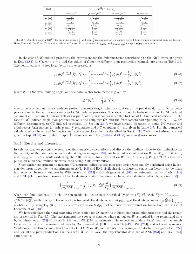
I(J) CR(NC ν(ν))

p −→ nπ+ p −→ pπ0 n −→ pπ− n −→ nπ0

32

( 32) 1√

3

f⋆

mπ

√

23

f⋆

mπ− 1√

3

f⋆

mπ

√

23

f⋆

mπ

32

( 12) 1√

3

f⋆

mπ

√

23

f⋆

mπ− 1√

3

f⋆

mπ

√

23

f⋆

mπ

12

( 32) − 1√

2

f⋆

mπ

12

f⋆

mπ

1√2

f⋆

mπ

12

f⋆

mπ

12

( 12) − 1√

2

f⋆

mπ

12

f⋆

mπ

1√2

f⋆

mπ

12

f⋆

mπ

Table 3.7: Coupling constant(CR) for spin and isospin 12

and spin 32

resonances for the charge current (anti)neutrino induced pion production.

Here f⋆ stands for R → Nπ coupling which is for ∆(1232) resonance is f∆Nπ and fR 12(fR 3

2) for spin 1

2( 32) resonances.

In the case of NC induced processes, the expressions for the different terms contributing to the NRB terms are givenin Eqs. (3.83)–(3.87), with a = 1 and the values of C for the different pion production channels are given in Table 3.5.The neural current vector form factors are expressed as:

f1,2(Q2)

for p−→ fp1,2(Q

2) =

(

1

2− 2 sin2 θW

)

fp1,2(Q

2)− 1

2fn1,2(Q

2) (3.96)

f1,2(Q2)

for n−→ fn1,2(Q

2) =

(

1

2− 2 sin2 θW

)

fn1,2(Q

2)− 1

2fp1,2(Q

2). (3.97)

where θW is the weak mixing angle, and the axial-vector form factor is given by

gp,n1 (Q2) = ±1

2g1(Q

2), (3.98)

where the plus (minus) sign stands for proton (neutron) target. The contribution of the pseudoscalar form factor beingproportional to the lepton mass vanishes for NC induced processes. The structure of the hadronic current for NC induceds-channel and u-channel spin as well as isospin 1

2 and 32 resonances is similar to that of CC induced reactions. In the

case of NC induced single pion production, only the couplings CR and the form factors corresponding to N −→ R aredifferent as compared to CC induced processes. In Section 3.3.7, we have already discussed in detail NC vector andaxial-vector form factors for spin 1

2 and 32 resonances and NC couplings CR are given in Table 3.7. For the numerical

calculations, we have used NC vector and axial-vector form factors described in Section 3.3.7 with the hadronic currentgiven in Eqs. (3.46) and (3.47) for spin 1

2 resonances and Eqs. (3.65) and (3.66) for spin 32 resonances.

3.4.3. Results and discussion

In this section, we present the results of the numerical calculations and discuss the findings. Due to the limitations onthe validity of the nonlinear sigma model at higher energies [134], we have put a constraint on W as Wmin = M +mπ

and Wmax = 1.2 GeV while evaluating the NRB terms. This constraint on W (i.e. M +mπ ≤ W ≤ 1.2GeV ) has beenput in all numerical evaluations while considering NRB contribution.

Since earlier experiments to measure CC neutrino induced single pion production were mainly performed using hydro-gen/deuteron target like the experiments at ANL [243] and BNL [244], therefore, deuteron correction factor must be takeninto account. In recent analyses by Wilkinson et al. [272] and Rodrigues et al. [280], experimental results of ANL [243]and BNL [244] have been normalized to the deuteron data. Therefore, we have taken deuteron effect by writing [140]:

(

dσ

dQ2dW

)

νd

=

∫

d~pdp|Ψd(~pdp)|2

M

Edp

(

dσ

dQ2dW

)

off shell

, (3.99)

where the four momentum of the proton inside the deuteron is described by pµ = (Edp , ~p

dp) with Ed

p (= MDeuteron −√

M2 + |~pdp|2) as the energy of the off shell proton inside the deuteron andM Deuteron is the deuteron mass.(

dσdQ2dW

)

off shellis obtained by using Eq. (3.2). In the above expression Ψd(~pd) is the deuteron wave function taken from the works ofLacombe et al. [281].

We have calculated the total scattering cross section for CC neutrino induced pion production processes and the resultsare presented in Fig. 3.5. The experimental data for π+p channel where no cut on W is applied is the reanalyzed databy Wilkinson et al. [272] of the ANL [243] and BNL [244] experiments. The experimental data for π0p and π+n channelsfor no cut on W are the reanalyzed data by Rodrigues et al. [280] of the ANL [243], BNL [244], and other experiments.While for all the three channels with a cut of 1.4 GeV on W , we have used the reanalyzed data by Rodrigues et al. [280]and for all the pion production channels with W < 1.6 GeV, the experimental data are of ANL [243] and BNL [244]experiments.

63

0

0.2

0.4

0.6

0.8

BNL extractedANL extracted

0

0.1

0.2

0.3

0.4

Full-FreeFull∆∆+B

0

0.1

0.2

0.3

0.4

0

0.1

0.2

0.3

0.4

0.5

0.6

σ(10

-38 c

m2 )

0

0.05

0.1

0.15

0

0.05

0.1

0.5 1 1.5 2Eν (GeV)

0

0.2

0.4

0.6

0.5 1 1.5 2Eν (GeV)

0

0.05

0.1

0.15

0.2

0.25

0.5 1 1.5 2Eν (GeV)

0

0.05

0.1

0.15

0.2

ANL 1982

pπ+

pπ+

pπ+

pπ0

pπ0

pπ0

nπ+

nπ+

nπ+

No Cut

No Cut No Cut

W<1.4 GeV

W<1.4 GeV W<1.4 GeV

W<1.6 GeVW<1.6 GeV W<1.6 GeV

Figure 3.5: Total scattering cross section for CC neutrino induced pion production processes: νµp −→ µ−pπ+ (left panel), νµn −→ µ−pπ0 (cen-tral panel), νµn −→ µ−nπ+ (right panel). The dashed line is the result calculated in the ∆(1232) dominance model, dashed-dotted line isthe result obtained when we include NRB terms in our calculations. The solid line is the result of our full calculation when other resonanceslike P11(1440), D13(1520), S11(1535), S31(1620), S11(1650), D33(1700) and P13(1720) are also included. All the above three cases are withdeuteron effect. The dotted line is the result of the full calculation without deuteron effect. The results in the top panels are obtained whenwe have not included any cut on the invariant mass. The middle panel shows the results with a cut of 1.4 GeV on the W , while in thebottom panel a cut of W < 1.6 GeV is introduced while calculating total scattering cross section. Data points quoted as ANL extracted andBNL extracted are the reanalyzed data by Wilkinson et al. [272] and Rodrigues et al. [280]. Other data points in figures are the results fromANL [243] experiment.

(i) In the case of νµp −→ µ−pπ+ induced reaction, the main contribution to the total scattering cross section comesfrom the ∆(1232) resonance when no cut on W is applied while when this cut is applied there is some contributionfrom the higher resonances and the background terms which are considered in this work. It should be noticed thatin the case when no cut on W is applied or when W < 1.4 GeV is considered, our theoretical results are in very goodagreement with the reanalyzed experimental data by Wilkinson et al. [272] and Rodrigues et al. [280]. While in thecase when W < 1.6 GeV cut is applied, we are consistent with the experimental data obtained by the ANL [243].Quantitatively, we find that due to the presence of the NRB terms there is an increase in the cross section whichis about 14% at Eνµ = 1 GeV which becomes ∼ 9% at Eνµ=2GeV, when no cut on W is applied. However, whenthe cuts on W are applied, then due to the presence of background contributions, this increase in the cross sectionfurther increases and become ∼ 13% at 2 GeV for W < 1.4 GeV and 12% for W < 1.6 GeV.

(ii) For νµn −→ µ−pπ0 as well as νµn −→ µ−nπ+ processes, there are significant contributions from the NRB termsas well as other higher resonant terms besides the ∆(1232) dominance. In the case of νµn −→ µ−pπ0 our resultswith deuteron effects are in a good agreement with the reanalyzed data as well as with the original data fromANL experiment at W < 1.6 GeV. Due to the presence of the background terms the total increase is about 32%at Eνµ = 1 GeV which becomes 20% at Eνµ = 2 GeV. With the inclusion of higher resonances, there is a furtherincrease of about 3% at Eνµ = 1 GeV and 40% at Eνµ = 2 GeV. It may be observed from the figure the our results

64

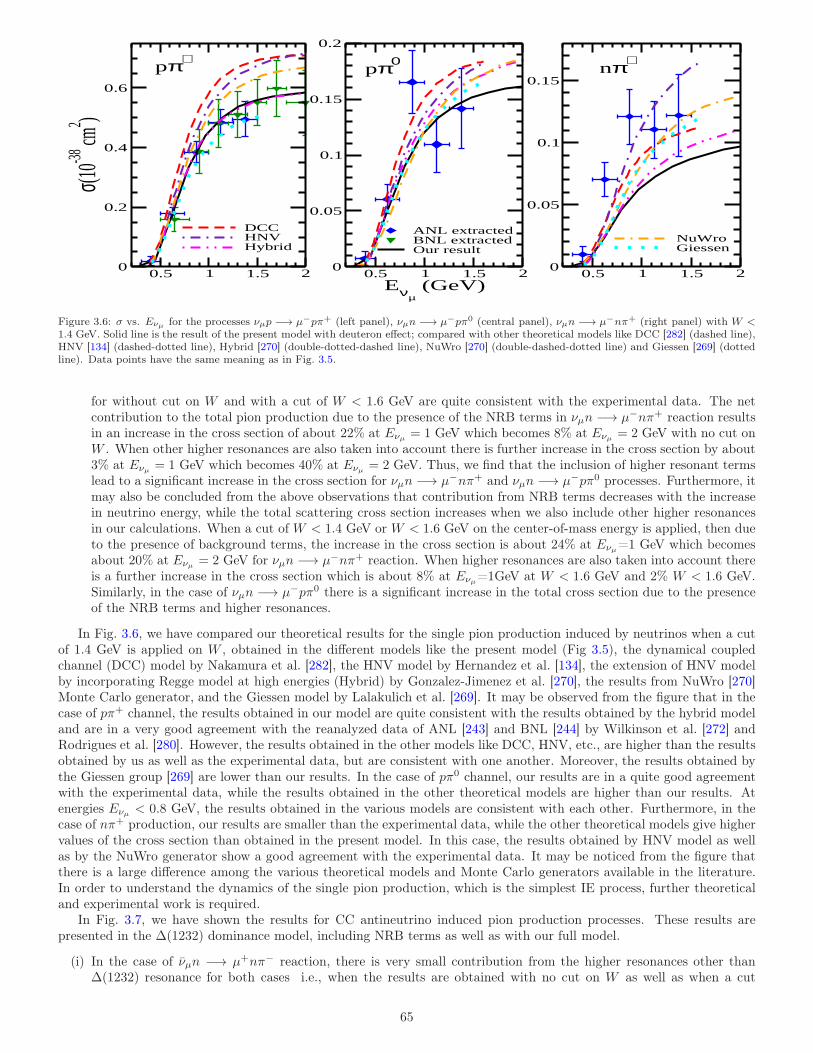
0.5 1 1.5 20

0.2

0.4

0.6σ(1

0-38 cm

2 )

ANL extractedBNL extractedOur result

0.5 1 1.5 2Eνµ

(GeV)0

0.05

0.1

0.15

0.2

DCCHNVHybrid

0.5 1 1.5 20

0.05

0.1

0.15

NuWroGiessen

pπ+pπ0 nπ+

Figure 3.6: σ vs. Eνµ for the processes νµp −→ µ−pπ+ (left panel), νµn −→ µ−pπ0 (central panel), νµn −→ µ−nπ+ (right panel) with W <1.4 GeV. Solid line is the result of the present model with deuteron effect; compared with other theoretical models like DCC [282] (dashed line),HNV [134] (dashed-dotted line), Hybrid [270] (double-dotted-dashed line), NuWro [270] (double-dashed-dotted line) and Giessen [269] (dottedline). Data points have the same meaning as in Fig. 3.5.

for without cut on W and with a cut of W < 1.6 GeV are quite consistent with the experimental data. The netcontribution to the total pion production due to the presence of the NRB terms in νµn −→ µ−nπ+ reaction resultsin an increase in the cross section of about 22% at Eνµ = 1 GeV which becomes 8% at Eνµ = 2 GeV with no cut onW . When other higher resonances are also taken into account there is further increase in the cross section by about3% at Eνµ = 1 GeV which becomes 40% at Eνµ = 2 GeV. Thus, we find that the inclusion of higher resonant termslead to a significant increase in the cross section for νµn −→ µ−nπ+ and νµn −→ µ−pπ0 processes. Furthermore, itmay also be concluded from the above observations that contribution from NRB terms decreases with the increasein neutrino energy, while the total scattering cross section increases when we also include other higher resonancesin our calculations. When a cut of W < 1.4 GeV or W < 1.6 GeV on the center-of-mass energy is applied, then dueto the presence of background terms, the increase in the cross section is about 24% at Eνµ=1 GeV which becomesabout 20% at Eνµ = 2 GeV for νµn −→ µ−nπ+ reaction. When higher resonances are also taken into account thereis a further increase in the cross section which is about 8% at Eνµ=1GeV at W < 1.6 GeV and 2% W < 1.6 GeV.Similarly, in the case of νµn −→ µ−pπ0 there is a significant increase in the total cross section due to the presenceof the NRB terms and higher resonances.

In Fig. 3.6, we have compared our theoretical results for the single pion production induced by neutrinos when a cutof 1.4 GeV is applied on W , obtained in the different models like the present model (Fig 3.5), the dynamical coupledchannel (DCC) model by Nakamura et al. [282], the HNV model by Hernandez et al. [134], the extension of HNV modelby incorporating Regge model at high energies (Hybrid) by Gonzalez-Jimenez et al. [270], the results from NuWro [270]Monte Carlo generator, and the Giessen model by Lalakulich et al. [269]. It may be observed from the figure that in thecase of pπ+ channel, the results obtained in our model are quite consistent with the results obtained by the hybrid modeland are in a very good agreement with the reanalyzed data of ANL [243] and BNL [244] by Wilkinson et al. [272] andRodrigues et al. [280]. However, the results obtained in the other models like DCC, HNV, etc., are higher than the resultsobtained by us as well as the experimental data, but are consistent with one another. Moreover, the results obtained bythe Giessen group [269] are lower than our results. In the case of pπ0 channel, our results are in a quite good agreementwith the experimental data, while the results obtained in the other theoretical models are higher than our results. Atenergies Eνµ < 0.8 GeV, the results obtained in the various models are consistent with each other. Furthermore, in thecase of nπ+ production, our results are smaller than the experimental data, while the other theoretical models give highervalues of the cross section than obtained in the present model. In this case, the results obtained by HNV model as wellas by the NuWro generator show a good agreement with the experimental data. It may be noticed from the figure thatthere is a large difference among the various theoretical models and Monte Carlo generators available in the literature.In order to understand the dynamics of the single pion production, which is the simplest IE process, further theoreticaland experimental work is required.

In Fig. 3.7, we have shown the results for CC antineutrino induced pion production processes. These results arepresented in the ∆(1232) dominance model, including NRB terms as well as with our full model.

(i) In the case of νµn −→ µ+nπ− reaction, there is very small contribution from the higher resonances other than∆(1232) resonance for both cases i.e., when the results are obtained with no cut on W as well as when a cut

65

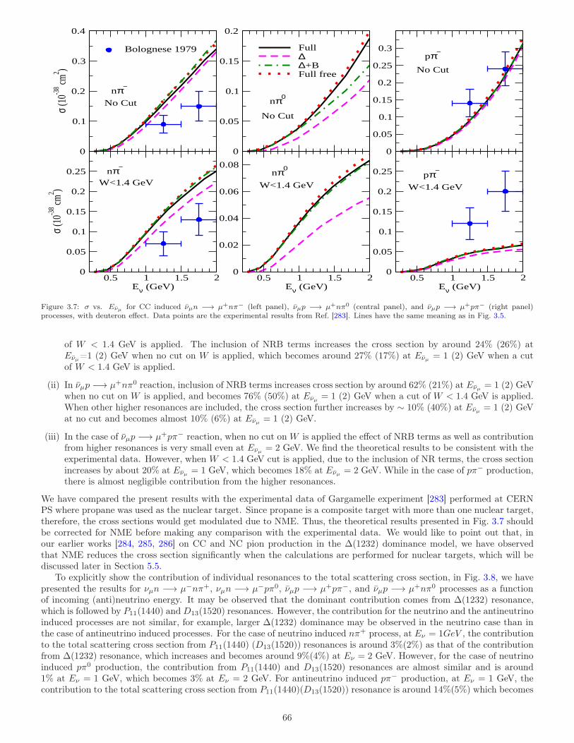
0

0.1

0.2

0.3

0.4

σ (10

-38 cm

2 )Bolognese 1979

0

0.05

0.1

0.15

0.2

Full∆∆+BFull free

0

0.05

0.1

0.15

0.2

0.25

0.3

0.5 1 1.5 2Eν (GeV)

0

0.05

0.1

0.15

0.2

0.25

σ (10

-38 cm

2 )

0.5 1 1.5 2Eν (GeV)

0

0.02

0.04

0.06

0.08

0.5 1 1.5 2Eν (GeV)

0

0.05

0.1

0.15

0.2

0.25

nπ−

nπ−

nπ0

nπ0

pπ−

pπ−

No Cut

No Cut

No Cut

W<1.4 GeV W<1.4 GeV W<1.4 GeV

Figure 3.7: σ vs. Eνµ for CC induced νµn −→ µ+nπ− (left panel), νµp −→ µ+nπ0 (central panel), and νµp −→ µ+pπ− (right panel)processes, with deuteron effect. Data points are the experimental results from Ref. [283]. Lines have the same meaning as in Fig. 3.5.

of W < 1.4 GeV is applied. The inclusion of NRB terms increases the cross section by around 24% (26%) atEνµ=1 (2) GeV when no cut on W is applied, which becomes around 27% (17%) at Eνµ = 1 (2) GeV when a cutof W < 1.4 GeV is applied.

(ii) In νµp −→ µ+nπ0 reaction, inclusion of NRB terms increases cross section by around 62% (21%) at Eνµ = 1 (2) GeVwhen no cut on W is applied, and becomes 76% (50%) at Eνµ = 1 (2) GeV when a cut of W < 1.4 GeV is applied.When other higher resonances are included, the cross section further increases by ∼ 10% (40%) at Eνµ = 1 (2) GeVat no cut and becomes almost 10% (6%) at Eνµ = 1 (2) GeV.

(iii) In the case of νµp −→ µ+pπ− reaction, when no cut on W is applied the effect of NRB terms as well as contributionfrom higher resonances is very small even at Eνµ = 2 GeV. We find the theoretical results to be consistent with theexperimental data. However, when W < 1.4 GeV cut is applied, due to the inclusion of NR terms, the cross sectionincreases by about 20% at Eνµ = 1 GeV, which becomes 18% at Eνµ = 2 GeV. While in the case of pπ− production,there is almost negligible contribution from the higher resonances.

We have compared the present results with the experimental data of Gargamelle experiment [283] performed at CERNPS where propane was used as the nuclear target. Since propane is a composite target with more than one nuclear target,therefore, the cross sections would get modulated due to NME. Thus, the theoretical results presented in Fig. 3.7 shouldbe corrected for NME before making any comparison with the experimental data. We would like to point out that, inour earlier works [284, 285, 286] on CC and NC pion production in the ∆(1232) dominance model, we have observedthat NME reduces the cross section significantly when the calculations are performed for nuclear targets, which will bediscussed later in Section 5.5.

To explicitly show the contribution of individual resonances to the total scattering cross section, in Fig. 3.8, we havepresented the results for νµn −→ µ−nπ+, νµn −→ µ−pπ0, νµp −→ µ+pπ−, and νµp −→ µ+nπ0 processes as a functionof incoming (anti)neutrino energy. It may be observed that the dominant contribution comes from ∆(1232) resonance,which is followed by P11(1440) and D13(1520) resonances. However, the contribution for the neutrino and the antineutrinoinduced processes are not similar, for example, larger ∆(1232) dominance may be observed in the neutrino case than inthe case of antineutrino induced processes. For the case of neutrino induced nπ+ process, at Eν = 1GeV , the contributionto the total scattering cross section from P11(1440) (D13(1520)) resonances is around 3%(2%) as that of the contributionfrom ∆(1232) resonance, which increases and becomes around 9%(4%) at Eν = 2 GeV. However, for the case of neutrinoinduced pπ0 production, the contribution from P11(1440) and D13(1520) resonances are almost similar and is around1% at Eν = 1 GeV, which becomes 3% at Eν = 2 GeV. For antineutrino induced pπ− production, at Eν = 1 GeV, thecontribution to the total scattering cross section from P11(1440)(D13(1520)) resonance is around 14%(5%) which becomes

66

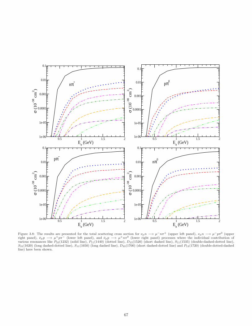
0.5 1 1.5 2Eν (GeV)

1e-06

1e-05

0.0001

0.001

0.01

0.1

σ (

10

-38 c

m2)

nπ+

0.5 1 1.5 2Eν (GeV)

1e-06

1e-05

0.0001

0.001

0.01

0.1

σ (

10

-38 c

m2)

pπ0

0.5 1 1.5 2Eν (GeV)

1e-06

1e-05

0.0001

0.001

0.01

0.1

σ (

10

-38 c

m2)

pπ−

0.5 1 1.5 2Eν (GeV)

1e-06

1e-05

0.0001

0.001

0.01

0.1

σ (

10

-38 c

m2)

nπ0

Figure 3.8: The results are presented for the total scattering cross section for νµn −→ µ−nπ+ (upper left panel), νµn −→ µ−pπ0 (upperright panel), νµp −→ µ+pπ− (lower left panel), and νµp −→ µ+nπ0 (lower right panel) processes where the individual contribution ofvarious resonances like P33(1232) (solid line), P11(1440) (dotted line), D13(1520) (short dashed line), S11(1535) (double-dashed-dotted line),S31(1620) (long dashed-dotted line), S11(1650) (long dashed line), D33(1700) (short dashed-dotted line) and P13(1720) (double-dotted-dashedline) have been shown.

67

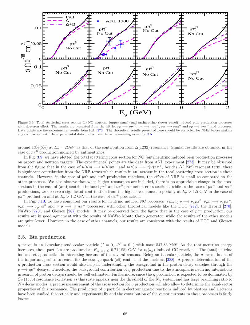
0

0.05

0.1σ (

10-3

8 cm2 )

Full∆∆+B

ANL 1980

0 10

0.05

0.1

0 1Eν (GeV)

0 1 0 1 2

pπ0

pπ− nπ0

nπ+

No Cut

No CutNo Cut

No Cut

nπ+

No CutNo Cut

nπ0pπ−

No CutNo Cutpπ0

Figure 3.9: Total scattering cross section for NC neutrino (upper panel) and antineutrino (lower panel) induced pion production processeswith deuteron effect. The results are presented from the left for νp −→ νpπ0, νn −→ νpπ−, νn −→ νnπ0 and νp −→ νnπ+ and processes.Data points are the experimental results from Ref. [273]. The theoretical results presented here should be corrected for NME before makingany comparison with the experimental data. Lines have the same meaning as in Fig. 3.5.

around 13%(5%) at Eν = 2GeV as that of the contribution from ∆(1232) resonance. Similar results are obtained in thecase of nπ0 production induced by antineutrinos.

In Fig. 3.9, we have plotted the total scattering cross section for NC (anti)neutrino induced pion production processeson proton and neutron targets. The experimental points are the data from ANL experiment [273]. It may be observedfrom the figure that in the case of ν(ν)n −→ ν(ν)pπ− and ν(ν)p −→ ν(ν)nπ+, besides ∆(1232) resonant term, thereis significant contribution from the NRB terms which results in an increase in the total scattering cross section in thesechannels. However, in the case of pπ0 and nπ0 production reactions, the effect of NRB is small as compared to theother processes. We also observe that when higher resonances are included, there is no appreciable change in the crosssections in the case of (anti)neutrino induced pπ0 and nπ0 production cross sections, while in the case of pπ− and nπ+

productions, we observe a significant contribution from the higher resonances, especially at Eν > 1.5 GeV in the case ofpπ− production and at Eν > 1.2 GeV in the case of nπ+ production.

In Fig. 3.10, we have compared our results for neutrino induced NC processes viz., νµp −→ νµpπ0, νµn −→ νµpπ

−,νµn −→ νµnπ

0 and νµp −→ νµnπ+ processes, with other theoretical models like the DCC [282], the Hybrid [270],

NuWro [270], and Giessen [287] models. It may be observed from the figure that in the case of pπ− production, ourresults are in good agreement with the results of NuWro Monte Carlo generator, while the results of the other modelsare quite lower. However, in the case of other channels, our results are consistent with the results of DCC and Giessenmodels.

3.5. Eta production

η-meson is an isoscalar pseudoscalar particle (I = 0, JP = 0−) with mass 547.86 MeV. As the (anti)neutrino energyincreases, these particles are produced at Eνl(νl) ≥ 0.71(.88) GeV for νe(νµ) induced CC reactions. The (anti)neutrinoinduced eta production is interesting because of the several reasons. Being an isoscalar particle, the η meson is one ofthe important probes to search for the strange quark (ss) content of the nucleons [288]. A precise determination of theη production cross section would also help in understanding the background in the proton decay searches through thep −→ ηe+ decays. Therefore, the background contribution of η production due to the atmospheric neutrino interactionsin search of proton decays should be well estimated. Furthermore, since the η production is expected to be dominated byS11(1535) resonance excitation as this state appears near the threshold of the Nη system and has large branching ratio toNη decay modes, a precise measurement of the cross section for η production will also allow to determine the axial-vectorproperties of this resonance. The production of η particle in electromagnetic reactions induced by photons and electronshave been studied theoretically and experimentally and the contribution of the vector currents to these processes is fairlyknown.

68

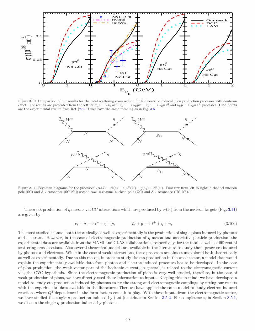
0 10

0.05

0.1

σ (10-38

cm2 )

Our resultDCCLAM

0 1

Eνµ (GeV)

ANL 1980HybridNuWro

0 1 0 1 2

pπ0

pπ−

nπ0

nπ+No Cut

No Cut

No Cut

No Cut

Figure 3.10: Comparison of our results for the total scattering cross section for NC neutrino induced pion production processes with deuteroneffect. The results are presented from the left for νµp −→ νµpπ0, νµn −→ νµpπ−, νµn −→ νµnπ0 and νµp −→ νµnπ+ processes. Data pointsare the experimental results from Ref. [273]. Lines have the same meaning as in Fig. 3.6.

W±

N

N

η

N

W±

N

S11

η

N

W±

N

N

η

N

W±

N

S11

η

N

Figure 3.11: Feynman diagrams for the processes ν/ν(k) +N(p) −→ µ∓(k′) + η(pη) +N ′(p′). First row from left to right: s-channel nucleonpole (SC) and S11 resonance (SC N∗); second row: u-channel nucleon pole (UC) and S11 resonance (UC N∗).

The weak production of η mesons via CC interactions which are produced by νl(νl) from the nucleon targets (Fig. 3.11)are given by

νℓ + n −→ l− + η + p, νℓ + p −→ l+ + η + n, (3.100)

The most studied channel both theoretically as well as experimentally is the production of single pions induced by photonsand electrons. However, in the case of electromagnetic production of η meson and associated particle production, theexperimental data are available from the MAMI and CLAS collaborations, respectively, for the total as well as differentialscattering cross sections. Also several theoretical models are available in the literature to study these processes inducedby photons and electrons. While in the case of weak interactions, these processes are almost unexplored both theoreticallyas well as experimentally. Due to this reason, in order to study the eta production in the weak sector, a model that wouldexplain the experimentally available data from photon and electron induced processes has to be developed. In the caseof pion production, the weak vector part of the hadronic current, in general, is related to the electromagnetic currentvia, the CVC hypothesis. Since the electromagnetic production of pions is very well studied, therefore, in the case ofweak production of pions, we have directly used those information as inputs. Keeping this in mind, we have developed amodel to study eta production induced by photons to fix the strong and electromagnetic couplings by fitting our resultswith the experimental data available in the literature. Then we have applied the same model to study electron inducedreactions where Q2 dependence in the form factors come into play. With these inputs from the electromagnetic sector,we have studied the single η production induced by (anti)neutrinos in Section 3.5.2. For completeness, in Section 3.5.1,we discuss the single η production induced by photons.

69

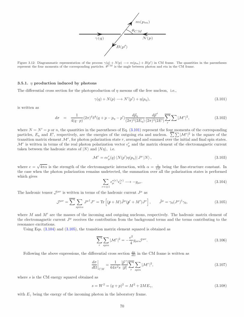
γ(q) N (p)

m(pm)

B(p′)

θCM

Figure 3.12: Diagrammatic representation of the process γ(q) + N(p) −→ m(pm) + B(p′) in CM frame. The quantities in the parenthesesrepresent the four momenta of the corresponding particles. θCM is the angle between photon and eta in the CM frame.

3.5.1. η production induced by photons

The differential cross section for the photoproduction of η mesons off the free nucleon, i.e.,

γ(q) +N(p) −→ N ′(p′) + η(pη), (3.101)

is written as

dσ =1

4(q · p) (2π)4δ4(q + p− pη − p′)

d~pη(2π)3(2Eη)

d~p ′

(2π)3(2E′)

∑

r

∑

|Mr|2, (3.102)

where N = N ′ = p or n, the quantities in the parentheses of Eq. (3.101) represent the four momenta of the correspondingparticles, Eη and E′, respectively, are the energies of the outgoing eta and nucleon.

∑∑ |Mr|2 is the square of thetransition matrix elementMr, for photon polarization state r, averaged and summed over the initial and final spin states.Mr is written in terms of the real photon polarization vector ǫrµ and the matrix element of the electromagnetic currenttaken between the hadronic states of |N〉 and |Nη〉, i.e.

Mr = eǫrµ(q) 〈N(p′)η(pη)| Jµ |N〉 , (3.103)

where e =√4πα is the strength of the electromagnetic interaction, with α = 1

137 being the fine-structure constant. Inthe case when the photon polarization remains undetected, the summation over all the polarization states is performedwhich gives

∑

r=±1

ǫ∗(r)µ ǫ(r)ν −→ −gµν . (3.104)

The hadronic tensor J µν is written in terms of the hadronic current Jµ as

J µν =∑ ∑

spins

Jµ†Jν = Tr[

(/p+M)Jµ(/p′ +M ′)Jν

]

, Jµ = γ0(Jµ)†γ0, (3.105)

where M and M ′ are the masses of the incoming and outgoing nucleons, respectively. The hadronic matrix element ofthe electromagnetic current Jµ receives the contribution from the background terms and the terms contributing to theresonance excitations.

Using Eqs. (3.104) and (3.105), the transition matrix element squared is obtained as

∑

r

∑

spin

|Mr|2 = −e2

4gµνJ µν . (3.106)

Following the above expressions, the differential cross section dσdΩ in the CM frame is written as

dσ

dΩ

∣

∣

∣

∣

CM

=1

64π2s

|~p ′||~p|∑

r

∑

spin

|Mr|2, (3.107)

where s is the CM energy squared obtained as

s =W 2 = (q + p)2 =M2 + 2MEγ , (3.108)

with Eγ being the energy of the incoming photon in the laboratory frame.

70

The hadronic currents for the various NR terms shown in Fig 3.11 (first row) are obtained using the nonlinear sigmamodel described in Section 3.3.1. The expressions of the hadronic currents for s-, u- channels are expressed as [134, 140]:

Jµ|sN = −As Fs(s)u(p′)/pηγ5

/p+ /q +M

s−M2

(

γµeN + iκN2M

σµνqν

)

u(p), (3.109)

Jµ|uN = −Au Fu(u)u(p′)(

γµeN + iκN2M

σµνqν

) /p′ − /q +M

u−M2 /pηγ5u(p), (3.110)

where N stands for a proton or a neutron in the initial and final states, s is defined in Eq. (3.108) and u = (p′− q)2, Ai’s;i = s, u are the coupling strengths of s, and u channels, respectively, and are obtained as

As = Au =

(

D − 3F

2√3fη

)

, (3.111)

D and F are the axial-vector couplings of the baryon octet and fη = 105 MeV is the η decay constant. The value of κfor proton, and neutron are κp = 1.793, and κn = −1.91 in units of µN .

In order to take into account the hadronic structure of the nucleons, the form factors Fs(s), and Fu(u), are introducedat the strong vertex. Various parameterizations of these form factors are available in the literature [289]. We use themost general form of the hadronic form factor which is taken to be of the dipole form [144]:

Fx(x) =Λ4B

Λ4B + (x −M2

x)2, x = s, u (3.112)

where ΛB is the cut-off parameter for the s- and u-channel NRB terms. The value of ΛB is fitted to the experimentaldata for both the proton and neutron targets simultaneously and the best fitted value is ΛB = 0.78 GeV for both s- andu-channel diagrams. x represents the Mandelstam variables s, u, and Mx =M corresponds to the mass of the exchangednucleons in the s and u channels. One of the most important property of the electromagnetic current is gauge invariancewhich corresponds to the current conservation and is implemented in the case of η production.

In Section 3.3.5, we have already discussed the structure of hadronic current contributing to spin 12 and 3

2 resonanceexcitations and their subsequent decays to meson-baryon final state. In the case of photon induced resonance excitations,the hadronic current is purely vector in nature. Since η is an isoscalar meson, therefore, it couples to spin 1

2 resonances only.The vertex function for positive and negative parity spin 1

2 resonances are given in Eqs. (3.30) and (3.30), respectively.In the case of real photons, which are purely transverse in nature i.e., the amplitude S 1

2= 0, the vector form factors are

expressed only in terms of A 12

helicity amplitude.

The explicit relation between the coupling FR+,R0

2 and the helicity amplitude Ap,n12

, in the limit Q2 = 0, is given by:

Ap,n12

=

√

2πα

M

(MR ∓M)2

M2R −M2

[

MR ±M2M

FR+,R0

2

]

, (3.113)

where the upper (lower) sign stands for the positive (negative) parity resonance. MR is the mass of correspondingresonance. In the case of η production, we have considered three spin 1

2 resonances viz. S11(1535), S11(1650), andP11(1710), where the dominant contribution to the total scattering cross section comes from S11(1535) resonance. In thepresent work, we have used the value of A 1

2for these resonances given in PDG [19].

The most general form of the hadronic currents for the s− and u− channel processes where a resonance state R12 is

produced and decays to a η and a nucleon in the final state, are written as

jµ∣

∣

s=

gRNη

fηu(p ′)/pηΓs

(

/p+ /q +MR

s−M2R + iMRΓR

)

Γµ12±u(p ), (3.114)

jµ∣

∣

u=

gRNη

fηu(p ′)Γµ

12±

(

/p′ − /q +MR

u−M2R + iMRΓR

)

/pηΓsu(p ),

where ΓR is the decay width of the resonance, Γs = 1(γ5) stands for the positive (negative) parity resonances. Γ 12+ and

Γ 12− are, respectively, the vertex function for the positive and negative parity resonances, defined in Eq. (3.30). gRNη is

the coupling strength for the process R→ Nη, given in Table 3.4.In analogy with the NR terms, we have considered the following form factors at the strong vertex, in order to take

into account the hadronic structure:

F ∗x (x) =

Λ4R

Λ4R + (x−M2

x)2, (3.115)

71

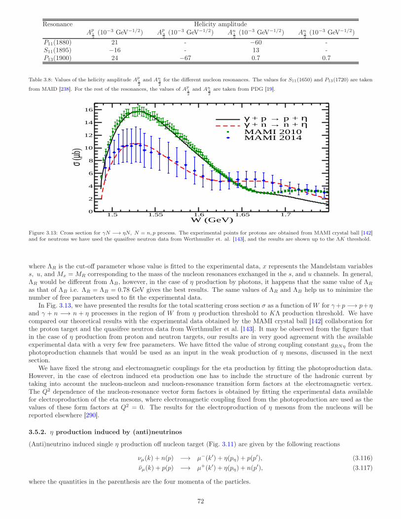
Resonance Helicity amplitude

Ap12

(10−3 GeV−1/2) Ap32

(10−3 GeV−1/2) An12

(10−3 GeV−1/2) An32

(10−3 GeV−1/2)

P11(1880) 21 - −60 -S11(1895) −16 - 13 -P13(1900) 24 −67 0.7 0.7

Table 3.8: Values of the helicity amplitude Ap12

and An32

for the different nucleon resonances. The values for S11(1650) and P13(1720) are taken

from MAID [238]. For the rest of the resonances, the values of Ap12

and An32

are taken from PDG [19].

1.5 1.55 1.6 1.65 1.7W (GeV)

0

2

4

6

8

10

12

14

16

σ (µb)

γ + p → p + ηγ + n → n + ηMAMI 2010MAMI 2014

Figure 3.13: Cross section for γN −→ ηN, N = n, p process. The experimental points for protons are obtained from MAMI crystal ball [142]and for neutrons we have used the quasifree neutron data from Werthmuller et. al. [143], and the results are shown up to the ΛK threshold.

where ΛR is the cut-off parameter whose value is fitted to the experimental data, x represents the Mandelstam variabless, u, and Mx =MR corresponding to the mass of the nucleon resonances exchanged in the s, and u channels. In general,ΛR would be different from ΛB, however, in the case of η production by photons, it happens that the same value of ΛR

as that of ΛB i.e. ΛR = ΛB = 0.78 GeV gives the best results. The same values of ΛR and ΛB help us to minimize thenumber of free parameters used to fit the experimental data.

In Fig. 3.13, we have presented the results for the total scattering cross section σ as a function of W for γ+p −→ p+ηand γ + n −→ n + η processes in the region of W from η production threshold to KΛ production threshold. We havecompared our theoretical results with the experimental data obtained by the MAMI crystal ball [142] collaboration forthe proton target and the quasifree neutron data from Werthmuller et al. [143]. It may be observed from the figure thatin the case of η production from proton and neutron targets, our results are in very good agreement with the availableexperimental data with a very few free parameters. We have fitted the value of strong coupling constant gRNη from thephotoproduction channels that would be used as an input in the weak production of η mesons, discussed in the nextsection.

We have fixed the strong and electromagnetic couplings for the eta production by fitting the photoproduction data.However, in the case of electron induced eta production one has to include the structure of the hadronic current bytaking into account the nucleon-nucleon and nucleon-resonance transition form factors at the electromagnetic vertex.The Q2 dependence of the nucleon-resonance vector form factors is obtained by fitting the experimental data availablefor electroproduction of the eta mesons, where electromagnetic coupling fixed from the photoproduction are used as thevalues of these form factors at Q2 = 0. The results for the electroproduction of η mesons from the nucleons will bereported elsewhere [290].

3.5.2. η production induced by (anti)neutrinos

(Anti)neutrino induced single η production off nucleon target (Fig. 3.11) are given by the following reactions

νµ(k) + n(p) −→ µ−(k′) + η(pη) + p(p′), (3.116)

νµ(k) + p(p) −→ µ+(k′) + η(pη) + n(p′), (3.117)

where the quantities in the parenthesis are the four momenta of the particles.

72

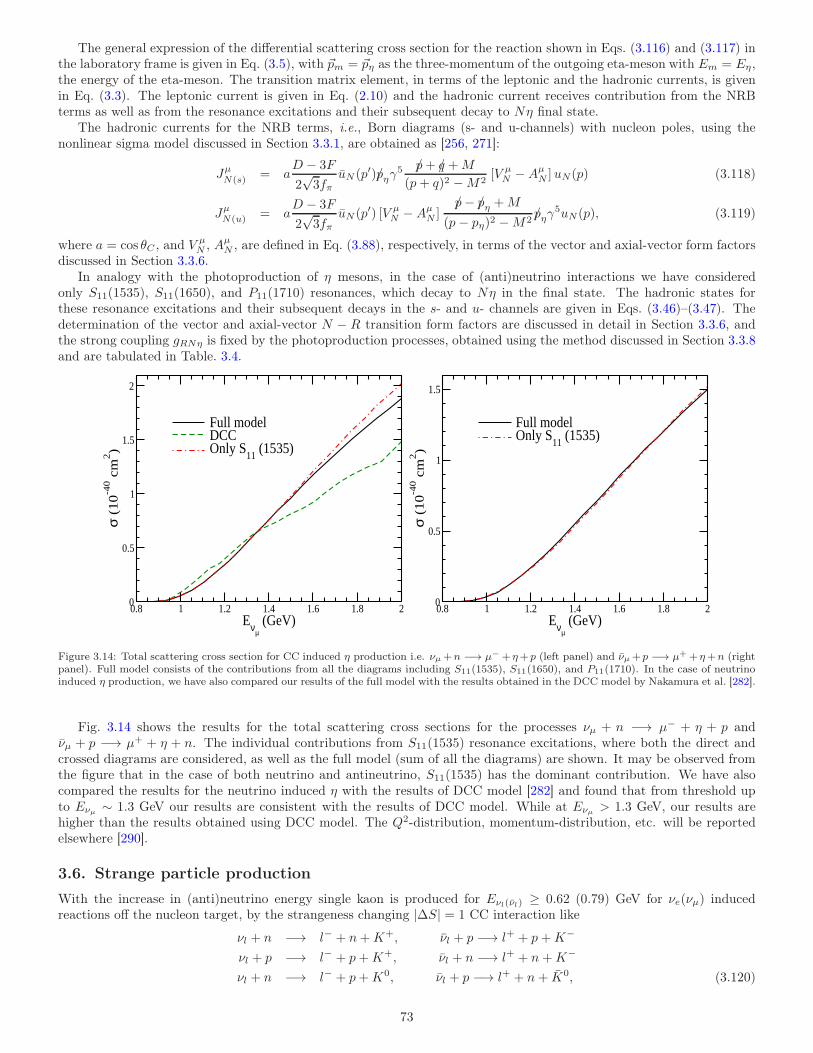
The general expression of the differential scattering cross section for the reaction shown in Eqs. (3.116) and (3.117) inthe laboratory frame is given in Eq. (3.5), with ~pm = ~pη as the three-momentum of the outgoing eta-meson with Em = Eη,the energy of the eta-meson. The transition matrix element, in terms of the leptonic and the hadronic currents, is givenin Eq. (3.3). The leptonic current is given in Eq. (2.10) and the hadronic current receives contribution from the NRBterms as well as from the resonance excitations and their subsequent decay to Nη final state.

The hadronic currents for the NRB terms, i.e., Born diagrams (s- and u-channels) with nucleon poles, using thenonlinear sigma model discussed in Section 3.3.1, are obtained as [256, 271]:

JµN(s) = a

D − 3F

2√3fπ

uN (p′)p/ηγ5 p/+ q/ +M

(p+ q)2 −M2[V µ

N −AµN ]uN(p) (3.118)

JµN(u) = a

D − 3F

2√3fπ

uN (p′) [V µN −A

µN ]

p/− p/η +M

(p− pη)2 −M2p/ηγ

5uN(p), (3.119)

where a = cos θC , and V µN , Aµ

N , are defined in Eq. (3.88), respectively, in terms of the vector and axial-vector form factorsdiscussed in Section 3.3.6.

In analogy with the photoproduction of η mesons, in the case of (anti)neutrino interactions we have consideredonly S11(1535), S11(1650), and P11(1710) resonances, which decay to Nη in the final state. The hadronic states forthese resonance excitations and their subsequent decays in the s- and u- channels are given in Eqs. (3.46)–(3.47). Thedetermination of the vector and axial-vector N − R transition form factors are discussed in detail in Section 3.3.6, andthe strong coupling gRNη is fixed by the photoproduction processes, obtained using the method discussed in Section 3.3.8and are tabulated in Table. 3.4.

0.8 1 1.2 1.4 1.6 1.8 2Eνµ

(GeV)0

0.5

1

1.5

2

σ (

10

-40 c

m2)

Full modelDCCOnly S

11 (1535)

0.8 1 1.2 1.4 1.6 1.8 2Eνµ

(GeV)0

0.5

1

1.5

σ (

10

-40 c

m2)

Full modelOnly S

11 (1535)

Figure 3.14: Total scattering cross section for CC induced η production i.e. νµ +n −→ µ− +η+p (left panel) and νµ+p −→ µ++η+n (rightpanel). Full model consists of the contributions from all the diagrams including S11(1535), S11(1650), and P11(1710). In the case of neutrinoinduced η production, we have also compared our results of the full model with the results obtained in the DCC model by Nakamura et al. [282].

Fig. 3.14 shows the results for the total scattering cross sections for the processes νµ + n −→ µ− + η + p andνµ + p −→ µ+ + η + n. The individual contributions from S11(1535) resonance excitations, where both the direct andcrossed diagrams are considered, as well as the full model (sum of all the diagrams) are shown. It may be observed fromthe figure that in the case of both neutrino and antineutrino, S11(1535) has the dominant contribution. We have alsocompared the results for the neutrino induced η with the results of DCC model [282] and found that from threshold upto Eνµ ∼ 1.3 GeV our results are consistent with the results of DCC model. While at Eνµ > 1.3 GeV, our results arehigher than the results obtained using DCC model. The Q2-distribution, momentum-distribution, etc. will be reportedelsewhere [290].

3.6. Strange particle production

With the increase in (anti)neutrino energy single kaon is produced for Eνl(νl) ≥ 0.62 (0.79) GeV for νe(νµ) inducedreactions off the nucleon target, by the strangeness changing |∆S| = 1 CC interaction like

νl + n −→ l− + n+K+, νl + p −→ l+ + p+K−

νl + p −→ l− + p+K+, νl + n −→ l+ + n+K−

νl + n −→ l− + p+K0, νl + p −→ l+ + n+ K0, (3.120)

73

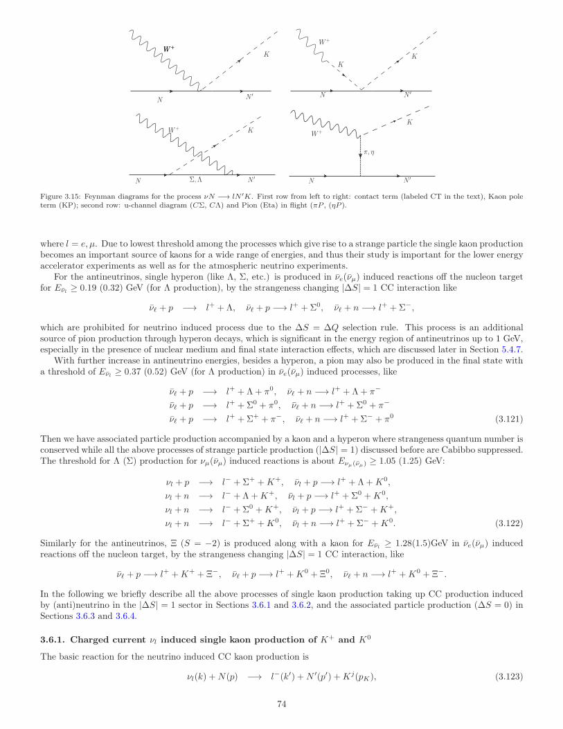
KW+

N N ′

W+W+

W+ K

N Σ, Λ N ′

N ′N

W+

KK

π, η

K

W+

N N ′

Figure 3.15: Feynman diagrams for the process νN −→ lN ′K. First row from left to right: contact term (labeled CT in the text), Kaon poleterm (KP); second row: u-channel diagram (CΣ, CΛ) and Pion (Eta) in flight (πP , (ηP ).

where l = e, µ. Due to lowest threshold among the processes which give rise to a strange particle the single kaon productionbecomes an important source of kaons for a wide range of energies, and thus their study is important for the lower energyaccelerator experiments as well as for the atmospheric neutrino experiments.

For the antineutrinos, single hyperon (like Λ, Σ, etc.) is produced in νe(νµ) induced reactions off the nucleon targetfor Eνl ≥ 0.19 (0.32) GeV (for Λ production), by the strangeness changing |∆S| = 1 CC interaction like

νℓ + p −→ l+ + Λ, νℓ + p −→ l+ +Σ0, νℓ + n −→ l+ +Σ−,

which are prohibited for neutrino induced process due to the ∆S = ∆Q selection rule. This process is an additionalsource of pion production through hyperon decays, which is significant in the energy region of antineutrinos up to 1 GeV,especially in the presence of nuclear medium and final state interaction effects, which are discussed later in Section 5.4.7.

With further increase in antineutrino energies, besides a hyperon, a pion may also be produced in the final state witha threshold of Eνl ≥ 0.37 (0.52) GeV (for Λ production) in νe(νµ) induced processes, like

νℓ + p −→ l+ + Λ+ π0, νℓ + n −→ l+ + Λ+ π−

νℓ + p −→ l+ +Σ0 + π0, νℓ + n −→ l+ +Σ0 + π−

νℓ + p −→ l+ +Σ+ + π−, νℓ + n −→ l+ +Σ− + π0 (3.121)

Then we have associated particle production accompanied by a kaon and a hyperon where strangeness quantum number isconserved while all the above processes of strange particle production (|∆S| = 1) discussed before are Cabibbo suppressed.The threshold for Λ (Σ) production for νµ(νµ) induced reactions is about Eνµ(νµ) ≥ 1.05 (1.25) GeV:

νl + p −→ l− +Σ+ +K+, νl + p −→ l+ + Λ+K0,

νl + n −→ l− + Λ+K+, νl + p −→ l+ +Σ0 +K0,

νl + n −→ l− +Σ0 +K+, νl + p −→ l+ +Σ− +K+,

νl + n −→ l− +Σ+ +K0, νl + n −→ l+ +Σ− +K0. (3.122)

Similarly for the antineutrinos, Ξ (S = −2) is produced along with a kaon for Eνl ≥ 1.28(1.5)GeV in νe(νµ) inducedreactions off the nucleon target, by the strangeness changing |∆S| = 1 CC interaction, like

νℓ + p −→ l+ +K+ + Ξ−, νℓ + p −→ l+ +K0 + Ξ0, νℓ + n −→ l+ +K0 + Ξ−.

In the following we briefly describe all the above processes of single kaon production taking up CC production inducedby (anti)neutrino in the |∆S| = 1 sector in Sections 3.6.1 and 3.6.2, and the associated particle production (∆S = 0) inSections 3.6.3 and 3.6.4.

3.6.1. Charged current νl induced single kaon production of K+ and K0

The basic reaction for the neutrino induced CC kaon production is

νl(k) +N(p) −→ l−(k′) +N ′(p′) +Kj(pK), (3.123)

74

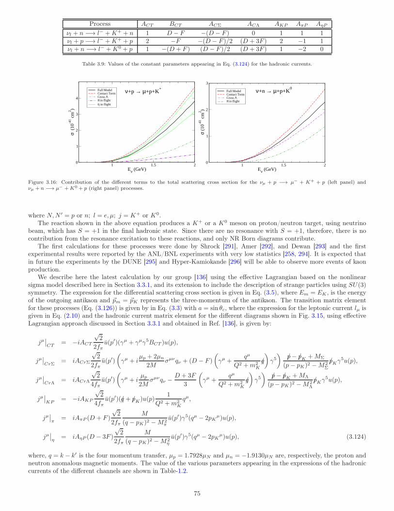
Process ACT BCT ACΣ ACΛ AKP AπP AηP

νl + n −→ l− +K+ + n 1 D − F −(D − F ) 0 1 1 1νl + p −→ l− +K+ + p 2 −F −(D − F )/2 (D + 3F ) 2 −1 1νl + n −→ l− +K0 + p 1 −(D + F ) (D − F )/2 (D + 3F ) 1 −2 0

Table 3.9: Values of the constant parameters appearing in Eq. (3.124) for the hadronic currents.

1 1.5 2Eν (GeV)

0

1

2

3

4

σ (

10-4

1 cm

2 )

Full ModelContact TermCross Λπ in flightη in flight

ν+p → µ+p+K+

1 1.5 2Eν (GeV)

0

1

2

3

σ (

10-4

1 cm

2 )

Full ModelContact TermCross Λπ in flight

ν+n → µ+p+K0

Figure 3.16: Contribution of the different terms to the total scattering cross section for the νµ + p −→ µ− + K+ + p (left panel) andνµ + n −→ µ− +K0 + p (right panel) processes.

where N,N ′ = p or n; l = e, µ; j = K+ or K0.The reaction shown in the above equation produces a K+ or a K0 meson on proton/neutron target, using neutrino

beam, which has S = +1 in the final hadronic state. Since there are no resonance with S = +1, therefore, there is nocontribution from the resonance excitation to these reactions, and only NR Born diagrams contribute.

The first calculations for these processes were done by Shrock [291], Amer [292], and Dewan [293] and the firstexperimental results were reported by the ANL/BNL experiments with very low statistics [258, 294]. It is expected thatin future the experiments by the DUNE [295] and Hyper-Kamiokande [296] will be able to observe more events of kaonproduction.

We describe here the latest calculation by our group [136] using the effective Lagrangian based on the nonlinearsigma model described here in Section 3.3.1, and its extension to include the description of strange particles using SU(3)symmetry. The expression for the differential scattering cross section is given in Eq. (3.5), where Em = EK , is the energyof the outgoing antikaon and ~pm = ~pK represents the three-momentum of the antikaon. The transition matrix elementfor these processes (Eq. (3.126)) is given by in Eq. (3.3) with a = sin θc, where the expression for the leptonic current lµ isgiven in Eq. (2.10) and the hadronic current matrix element for the different diagrams shown in Fig. 3.15, using effectiveLagrangian approach discussed in Section 3.3.1 and obtained in Ref. [136], is given by:

jµ∣

∣

CT= −iACT

√2

2fπu(p′)(γµ + γµγ5BCT )u(p),

jµ∣

∣

CrΣ= iACrΣ

√2

2fπu(p′)

(

γµ + iµp + 2µn

2Mσµνqν + (D − F )

(

γµ +qµ

Q2 +m2K

q/

)

γ5)

p/− p/K +MΣ

(p− pK)2 −M2Σ

p/Kγ5u(p),

jµ∣

∣

CrΛ= iACrΛ

√2

4fπu(p′)

(

γµ + iµp

2Mσµνqν −

D + 3F

3

(

γµ +qµ

Q2 +m2K

q/

)

γ5)

p/− p/K +MΛ

(p− pK)2 −M2Λ

p/Kγ5u(p),

jµ∣

∣

KP= −iAKP

√2

4fπu(p′)(q/ + p/K)u(p)

1

Q2 +m2K

qµ,

jµ∣

∣

π= iAπP (D + F )

√2

2fπ

M

(q − pK)2 −M2π

u(p′)γ5(qµ − 2pKµ)u(p),

jµ∣

∣

η= iAηP (D − 3F )

√2

2fπ

M

(q − pK)2 −M2η

u(p′)γ5(qµ − 2pKµ)u(p), (3.124)

where, q = k − k′ is the four momentum transfer, µp = 1.7928µN and µn = −1.9130µN are, respectively, the proton andneutron anomalous magnetic moments. The value of the various parameters appearing in the expressions of the hadroniccurrents of the different channels are shown in Table-1.2.

75

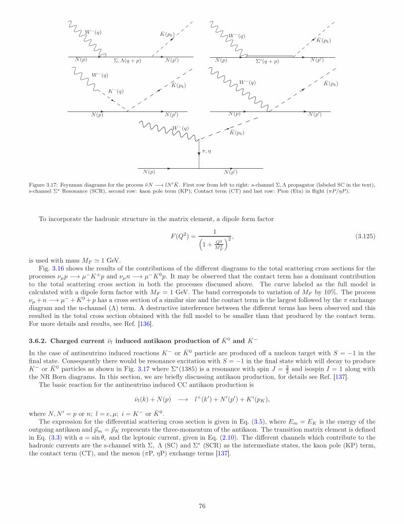
N(p′)

W−(q)

Σ∗(q + p)N(p) N(p′)

W−(q)K(pk)

N(p′)

K(pk)W−(q)

N(p)

Σ, Λ(q + p)N(p) N(p′)

K(pk)

N(p′)N(p)

W−(q)

K(pk)K−(q)

π, η

N(p)

W−(q)K(pk)

Figure 3.17: Feynman diagrams for the process νN −→ lN ′K. First row from left to right: s-channel Σ,Λ propagator (labeled SC in the text),s-channel Σ∗ Resonance (SCR), second row: kaon pole term (KP); Contact term (CT) and last row: Pion (Eta) in flight (πP/ηP ).

To incorporate the hadronic structure in the matrix element, a dipole form factor

F (Q2) =1

(

1 + Q2

M2F

)2 , (3.125)

is used with mass MF ≃ 1 GeV.Fig. 3.16 shows the results of the contributions of the different diagrams to the total scattering cross sections for the

processes νµp −→ µ−K+p and νµn −→ µ−K0p. It may be observed that the contact term has a dominant contributionto the total scattering cross section in both the processes discussed above. The curve labeled as the full model iscalculated with a dipole form factor with MF = 1 GeV. The band corresponds to variation of MF by 10%. The processνµ+n −→ µ−+K0+p has a cross section of a similar size and the contact term is the largest followed by the π exchangediagram and the u-channel (Λ) term. A destructive interference between the different terms has been observed and thisresulted in the total cross section obtained with the full model to be smaller than that produced by the contact term.For more details and results, see Ref. [136].

3.6.2. Charged current νl induced antikaon production of K0 and K−

In the case of antineutrino induced reactions K− or K0 particle are produced off a nucleon target with S = −1 in thefinal state. Consequently there would be resonance excitation with S = −1 in the final state which will decay to produceK− or K0 particles as shown in Fig. 3.17 where Σ∗(1385) is a resonance with spin J = 3

2 and isospin I = 1 along withthe NR Born diagrams. In this section, we are briefly discussing antikaon production, for details see Ref. [137].

The basic reaction for the antineutrino induced CC antikaon production is

νl(k) +N(p) −→ l+(k′) +N ′(p′) +Ki(pK),

where N,N ′ = p or n; l = e, µ; i = K− or K0.The expression for the differential scattering cross section is given in Eq. (3.5), where Em = EK is the energy of the

outgoing antikaon and ~pm = ~pK represents the three-momentum of the antikaon. The transition matrix element is definedin Eq. (3.3) with a = sin θc and the leptonic current, given in Eq. (2.10). The different channels which contribute to thehadronic currents are the s-channel with Σ, Λ (SC) and Σ∗ (SCR) as the intermediate states, the kaon pole (KP) term,the contact term (CT), and the meson (πP, ηP) exchange terms [137].

76

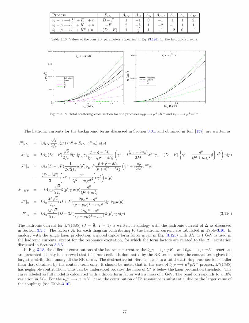
Process BCT ACT AΣ AΛ AKP Aπ Aη AΣ∗

νl + n −→ l+ +K− + n D − F 1 −1 0 −1 1 1 2νl + p −→ l+ +K− + p −F 2 − 1

2 1 −2 −1 1 1νl + p −→ l+ + K0 + n −(D + F ) 1 1

2 1 −1 −2 0 −1

Table 3.10: Values of the constant parameters appearing in Eq. (3.126) for the hadronic currents.

0.8 1 1.2 1.4 1.6 1.8 2

Eν (GeV)

0

1e-41

2e-41

3e-41

4e-41

σ (c

m2 )

Full ModelContactπΛΣ∗

ν µ p → µ+ p K

−

1 1.5 2Eν (GeV)

0

5e-42

1e-41

σ (c

m2 )

Full ModelContactπΣ∗

ν µ n → µ+ n K

−

Figure 3.18: Total scattering cross section for the processes νµp −→ µ+pK− and νµn −→ µ+nK−.

The hadronic currents for the background terms discussed in Section 3.3.1 and obtained in Ref. [137], are written as

Jµ|CT = iACT

√2

2fπu(p′) (γµ +BCT γµγ5) u(p)

Jµ|Σ = iAΣ(D − F )√2

2fπu(p′)/pKγ5

p/+ q/ +MΣ

(p+ q)2 −M2Σ

(

γµ + i(µp + 2µn)

2Mσµνqν + (D − F )

γµ +qµ

Q2 +mK2q/

γ5)

u(p)

Jµ|Λ = iAΛ(D + 3F )1

2√2fπ

u(p′)/pKγ5 p/+ q/+MΛ

(p+ q)2 −M2Λ

(

γµ + iµp

2Mσµνqν

− (D + 3F )

3

γµ +qµ

Q2 +mK2q/

γ5)

u(p)

Jµ|KP = −iAKP

√2

2fπu(p′)q/ u(p)

qµ

Q2 +m2K

Jµ|π = iAπM√2

2fπ(D + F )

2pKµ − qµ

(q − pK)2 −mπ2u(p′)γ5u(p)

Jµ|η = iAηM√2

2fπ(D − 3F )

2pKµ − qµ

(q − pK)2 −mη2u(p′)γ5u(p) (3.126)

The hadronic current for Σ∗(1385) (J = 32 , I = 1) is written in analogy with the hadronic current of ∆ as discussed

in Section 3.3.5. The factors Ai for each diagram contributing to the hadronic current are tabulated in Table-3.10. Inanalogy with the single kaon production, a global dipole form factor given in Eq. (3.125) with MF ≃ 1 GeV is used inthe hadronic currents, except for the resonance excitation, for which the form factors are related to the ∆+ excitationdiscussed in Section 3.3.5.

In Fig. 3.18, the different contributions of the hadronic current to the νµp −→ µ+pK− and νµn −→ µ+nK− reactionsare presented. It may be observed that the cross section is dominated by the NR terms, where the contact term gives thelargest contribution among all the NR terms. The destructive interference leads to a total scattering cross section smallerthan that obtained by the contact term only. It should be noted that in the case of νµp −→ µ+pK− process, Σ∗(1385)has negligible contribution. This can be understood because the mass of Σ∗ is below the kaon production threshold. Thecurve labeled as full model is calculated with a dipole form factor with a mass of 1 GeV. The band corresponds to a 10%variation in MF . For the νµn −→ µ+nK− case, the contribution of Σ∗ resonance is substantial due to the larger value ofthe couplings (see Table-3.10).

77

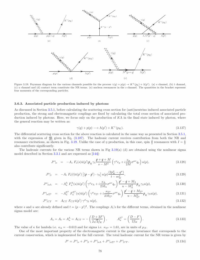
p(p)

γ(q)

p(p + q) Λ(p′)

K+(pK)

(a)

p(p)

K+(p− p′)

Λ(p′)

K+(pK)

γ(q)

(b)

p(p)

γ(q)

Λ,Σ0(p′ − q) Λ(p′)

K+(pK)

(c)

p(p)

γ(q)

Λ(p′)

K+(pK)

(d)

p(p)

γ(q)

N⋆(p + q) Λ(p′)

K+(pK)

(e)

Figure 3.19: Feynman diagram for the various channels possible for the process γ(q) + p(p) → K+(pk) + Λ(p′). (a) s channel, (b) t channel,(c) u channel and (d) contact term constitute the NR terms. (e) nucleon resonances in the s channel. The quantities in the bracket representfour momenta of the corresponding particles.

3.6.3. Associated particle production induced by photons

As discussed in Section 3.5.1, before calculating the scattering cross section for (anti)neutrino induced associated particleproduction, the strong and electromagnetic couplings are fixed by calculating the total cross section of associated pro-duction induced by photons. Here, we focus only on the production of KΛ in the final state induced by photon, wherethe general reaction may be written as:

γ(q) + p(p) −→ Λ(p′) +K+(pK). (3.127)

The differential scattering cross section for the above reaction is calculated in the same way as presented in Section 3.5.1,with the expression of dσ

dΩ given in Eq. (3.107). The hadronic current receives contribution from both the NR andresonance excitations, as shown in Fig. 3.19. Unlike the case of η production, in this case, spin 3

2 resonances with I = 12

also contribute significantly.The hadronic currents for the various NR terms shown in Fig 3.19(a)–(d) are obtained using the nonlinear sigma

model described in Section 3.3.1 and are expressed as [144]:

Jµ|s = −As Fs(s)u(p′)/pKγ5

/p+ /q +M

s−M2

(

γµep + iκp2M

σµνqν

)

u(p), (3.128)

Jµ|t = −At Ft(t)u(p′)[

(/p− /p′) · γ5]

u(p)(2pµK − qµ)t−m2

K

, (3.129)

Jµ|uΛ = −AΛu FΛ

u (u)u(p′)

(

γµeΛ + iκΛ2MΛ

σµνqν

)

/p′ − /q +MΛ

u−M2Λ

/pKγ5u(p), (3.130)

Jµ|uΣ0 = −AΣ0

u FΣ0

u (u)u(p′)

(

γµeΣ0 + iκΣ0

2MΣ0

σµνqν

)

/p′ − /q +MΣ0

u−M2Σ0

/pKγ5u(p), (3.131)

Jµ|CT = ACT FCT u(p′) γµγ5 u(p), (3.132)

where s and u are already defined and t = (p− p′)2. The couplings Ai’s for the different terms, obtained in the nonlinearsigma model are:

As = At = AΛu = ACT = −

(

D + 3F

2√3fK

)

, AΣ0

u =

(

D − F2fK

)

. (3.133)

The value of κ for lambda i.e. κΛ = −0.613 and for sigma i.e. κΣ0 = 1.61, are in units of µN .One of the most important property of the electromagnetic current is the gauge invariance that corresponds to the

current conservation, which is implemented for the full current. The total hadronic current for the NR terms is given by

Jµ = Jµ|s + Jµ|t + Jµ|uΛ + Jµ|uΣ0 + Jµ|CT . (3.134)

78

The condition to fulfill gauge invariance is qµJµ = 0, which gives

qµJµ = −D + F

2√3fK

u(p′)[

(/pkFs + (/p′ − /p)Ft − /qFCT )γ5

]

u(p). (3.135)

From the above equation, it is evident that the hadronic current is not gauge invariant. Therefore, in order to restoregauge invariance, the following term is added to Eq. (3.135)

qµJµadd = −D + F

2√3fK

u(p′)[

/pk (FCT − Fs) + (/p′ − /p)(FCT − Ft)

]

γ5u(p). (3.136)

Thus, the presence of the additional terms given in Eq. (3.136) implies that the gauge invariance can be achieved if thehadronic current Jµ is supplemented by adding an additional term Jµ

add given by

Jµadd = −D + F

2√3fK

u(p′)

[

2/pkpµ

s−M2(FCT − Fs) +

2pµkt−M2

k

(/p− /p′)(FCT − Ft)

]

u(p). (3.137)

In order to take into account the effect of the form factor for the contact term, there are different prescriptions availablein the literature, for example that of Ohta [297], Haberzettl et al. [298], Davidson and Workman[299], etc. In the presentwork, we have followed the prescription of Davidson and Workman [299], where FCT is given by:

FCT = Fs(s) + Ft(t)− Fs(s)× Ft(t). (3.138)

In the case of associated particle production, we have considered six nucleon resonances exchanged in the s channel, out ofwhich four are spin 1

2 viz. S11(1650), P11(1710), P11(1880), and S11(1895), and two are spin 32 resonances viz. P13(1720),

and P13(1900). We have already discussed the case of spin 12 resonances in Section 3.5.1. However, for completeness, in

this section we write the general form of the hadronic currents for the s channel processes where a resonance state withspin 1

2 is produced and decays to a kaon and a lambda in the final state, are written as [144]

jµ∣

∣

12±R

= − u(p ′)gRKΛ

fK/pKΓs

/p+ /q +MR

s−M2R + iMRΓR

Γµ12±u(p ), (3.139)

where ΓR is the decay width of the resonance, Γs = 1(γ5) stands for the positive (negative) parity resonances. Γ 12+ and

Γ 12− are, respectively, the vertex function for the positive and negative parity resonances, defined in Eq. (3.30). gRKΛ is

the coupling strength for the process R→ KΛ, given in Table 3.4. For a more detailed discussion, see Ref. [144].In the following, we briefly discuss spin 3

2 resonance excitations. The general structure of the hadronic current forN − R transition has already been discussed in Section 3.3.5. In the case of real photon scattering, the electromagneticcouplings Cp,n

i are related to the helicity amplitudes A 12, A 3

2and S 1

2, which are obtained using Eqs. (3.55)–(3.57) in the

limit Q2 = 0. In the numerical calculations, we have taken S 12= 0 as we are dealing with the real photons. The fitted

values of A 12

and A 32

have been taken from PDG [19] for spin 12 and 3

2 resonances, and are quoted in Table 3.2.

The most general expression of the hadronic current for the s channel spin 32 resonance exchange may be written

as [144]:

jµ∣

∣

32±R

= iegRKΛ

fK

pαKΓs

s−M2R + iMRΓR

u(p ′)P3/2αβ (pR)Γ

βµ32±u(p ), pR = p+ q, (3.140)

where Γs = 1(γ5) for positive (negative) parity resonances, fK is defined in Section 3.3.8, gRKΛ is the coupling strengthfor R → KΛ transition, the values of which are given in Table 3.4. MR is the mass of the resonance, ΓR is its decay

width and P3/2αβ (pR) is given in Eq. (3.67).

In Fig. 3.20, we have presented the results for the total scattering cross section as a function ofW for the photon inducedKΛ production. The theoretical calculations are compared with the experimental data from the CLAS experiment [145].It may be observed from the figure that there is good agreement of our results with the experimental data.

3.6.4. Associated particle production induced by (anti)neutrinos

The study of the neutrino induced ∆S = 0 associated particle production processes provide an improved understandingof the basic symmetries of the SM, structure of the weak hadronic form factors, strange-quark content of the nucleon,coupling constants, etc. Moreover the kaon production through the associated production also constitutes a backgroundin the proton decay searches i.e. p −→ Kν. Therefore, an understanding and reliable estimate of the cross sections for theneutrino induced kaon production contributing as the background event is important and has been emphasized [300, 301].The experimental observations of the neutrino induced associated particle production processes were performed earlier

79

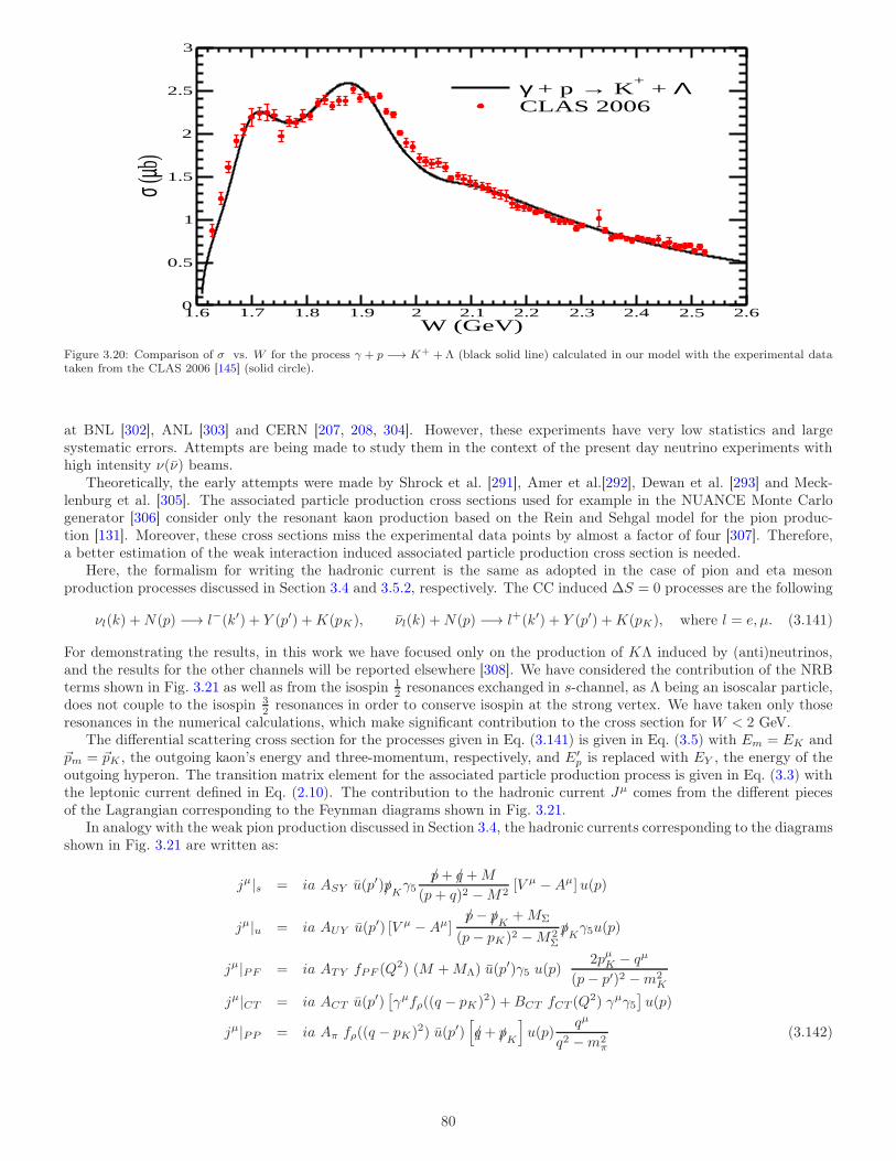
1.6 1.7 1.8 1.9 2 2.1 2.2 2.3 2.4 2.5 2.6W (GeV)

0

0.5

1

1.5

2

2.5

3

σ (µb)

γ + p → K+ + Λ

CLAS 2006

Figure 3.20: Comparison of σ vs. W for the process γ + p −→ K+ +Λ (black solid line) calculated in our model with the experimental datataken from the CLAS 2006 [145] (solid circle).

at BNL [302], ANL [303] and CERN [207, 208, 304]. However, these experiments have very low statistics and largesystematic errors. Attempts are being made to study them in the context of the present day neutrino experiments withhigh intensity ν(ν) beams.

Theoretically, the early attempts were made by Shrock et al. [291], Amer et al.[292], Dewan et al. [293] and Meck-lenburg et al. [305]. The associated particle production cross sections used for example in the NUANCE Monte Carlogenerator [306] consider only the resonant kaon production based on the Rein and Sehgal model for the pion produc-tion [131]. Moreover, these cross sections miss the experimental data points by almost a factor of four [307]. Therefore,a better estimation of the weak interaction induced associated particle production cross section is needed.

Here, the formalism for writing the hadronic current is the same as adopted in the case of pion and eta mesonproduction processes discussed in Section 3.4 and 3.5.2, respectively. The CC induced ∆S = 0 processes are the following

νl(k) +N(p) −→ l−(k′) + Y (p′) +K(pK), νl(k) +N(p) −→ l+(k′) + Y (p′) +K(pK), where l = e, µ. (3.141)

For demonstrating the results, in this work we have focused only on the production of KΛ induced by (anti)neutrinos,and the results for the other channels will be reported elsewhere [308]. We have considered the contribution of the NRBterms shown in Fig. 3.21 as well as from the isospin 1

2 resonances exchanged in s-channel, as Λ being an isoscalar particle,does not couple to the isospin 3

2 resonances in order to conserve isospin at the strong vertex. We have taken only thoseresonances in the numerical calculations, which make significant contribution to the cross section for W < 2 GeV.

The differential scattering cross section for the processes given in Eq. (3.141) is given in Eq. (3.5) with Em = EK and~pm = ~pK , the outgoing kaon’s energy and three-momentum, respectively, and E′

p is replaced with EY , the energy of theoutgoing hyperon. The transition matrix element for the associated particle production process is given in Eq. (3.3) withthe leptonic current defined in Eq. (2.10). The contribution to the hadronic current Jµ comes from the different piecesof the Lagrangian corresponding to the Feynman diagrams shown in Fig. 3.21.

In analogy with the weak pion production discussed in Section 3.4, the hadronic currents corresponding to the diagramsshown in Fig. 3.21 are written as:

jµ|s = ia ASY u(p′)/pKγ5p/+ q/+M

(p+ q)2 −M2[V µ −Aµ]u(p)

jµ|u = ia AUY u(p′) [V µ −Aµ]p/− /pK +MΣ

(p− pK)2 −M2Σ/pKγ5u(p)

jµ|PF = ia ATY fPF (Q2) (M +MΛ) u(p

′)γ5 u(p)2pµK − qµ

(p− p′)2 −m2K

jµ|CT = ia ACT u(p′)[

γµfρ((q − pK)2) +BCT fCT (Q2) γµγ5

]

u(p)

jµ|PP = ia Aπ fρ((q − pK)2) u(p′)[

q/+ /pK

]

u(p)qµ

q2 −m2π

(3.142)

80

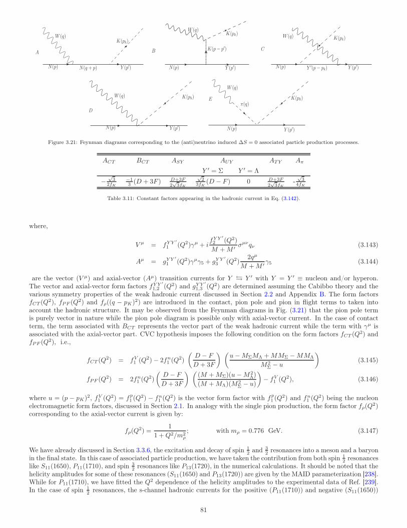
N(q + p)N(p) Y (p′)

W (q)K(pk)

K(p − p′)

N(p) Y (p′)

W (q)K(pk)

Y ′(p − pk)N(p) Y (p′)

W (q) K(pk)

A B C

Y (p′)

K(pk)W (q)

N(p)

D

W (q)

Y (p′)N(p)

K(pk)π(q)

E

Figure 3.21: Feynman diagrams corresponding to the (anti)neutrino induced ∆S = 0 associated particle production processes.

ACT BCT ASY AUY ATY Aπ

Y ′ = Σ Y ′ = Λ

−√3

2fK−13 (D + 3F ) D+3F

2√3fK

√2

3fK(D − F ) 0 D+3F

2√3fK

-√3

4fK

Table 3.11: Constant factors appearing in the hadronic current in Eq. (3.142).

where,

V µ = fY Y ′

1 (Q2)γµ + ifY Y ′

2 (Q2)

M +M ′ σµνqν (3.143)

Aµ = gY Y ′

1 (Q2)γµγ5 + gY Y ′

3 (Q2)2qµ

M +M ′ γ5 (3.144)

are the vector (V µ) and axial-vector (Aµ) transition currents for Y Y ′ with Y = Y ′ ≡ nucleon and/or hyperon.The vector and axial-vector form factors fY Y ′

1,2 (Q2) and gY Y ′

1,3 (Q2) are determined assuming the Cabibbo theory and thevarious symmetry properties of the weak hadronic current discussed in Section 2.2 and Appendix B. The form factorsfCT (Q

2), fPF (Q2) and fρ((q − pK)2) are introduced in the contact, pion pole and pion in flight terms to taken into

account the hadronic structure. It may be observed from the Feynman diagrams in Fig. (3.21) that the pion pole termis purely vector in nature while the pion pole diagram is possible only with axial-vector current. In the case of contactterm, the term associated with BCT represents the vector part of the weak hadronic current while the term with γµ isassociated with the axial-vector part. CVC hypothesis imposes the following condition on the form factors fCT (Q

2) andfPF (Q

2), i.e.,

fCT (Q2) = fV

1 (Q2)− 2fn1 (Q

2)

(

D − FD + 3F

) (

u−MΣMΛ +MMΣ −MMΛ

M2Σ − u

)

(3.145)

fPF (Q2) = 2fn

1 (Q2)

(

D − FD + 3F

) (

(M +MΣ)(u −M2Λ)

(M +MΛ)(M2Σ − u)

)

− fV1 (Q2), (3.146)

where u = (p − pK)2, fV1 (Q2) = fp

1 (Q2) − fn

1 (Q2) is the vector form factor with fp

1 (Q2) and fn

1 (Q2) being the nucleon

electromagnetic form factors, discussed in Section 2.1. In analogy with the single pion production, the form factor fρ(Q2)

corresponding to the axial-vector current is given by:

fρ(Q2) =

1

1 +Q2/m2ρ

; with mρ = 0.776 GeV. (3.147)

We have already discussed in Section 3.3.6, the excitation and decay of spin 12 and 3

2 resonances into a meson and a baryonin the final state. In this case of associated particle production, we have taken the contribution from both spin 1

2 resonanceslike S11(1650), P11(1710), and spin 3

2 resonances like P13(1720), in the numerical calculations. It should be noted that thehelicity amplitudes for some of these resonances (S11(1650) and P13(1720)) are given by the MAID parameterization [238].While for P11(1710), we have fitted the Q2 dependence of the helicity amplitudes to the experimental data of Ref. [239].In the case of spin 1

2 resonances, the s-channel hadronic currents for the positive (P11(1710)) and negative (S11(1650))

81

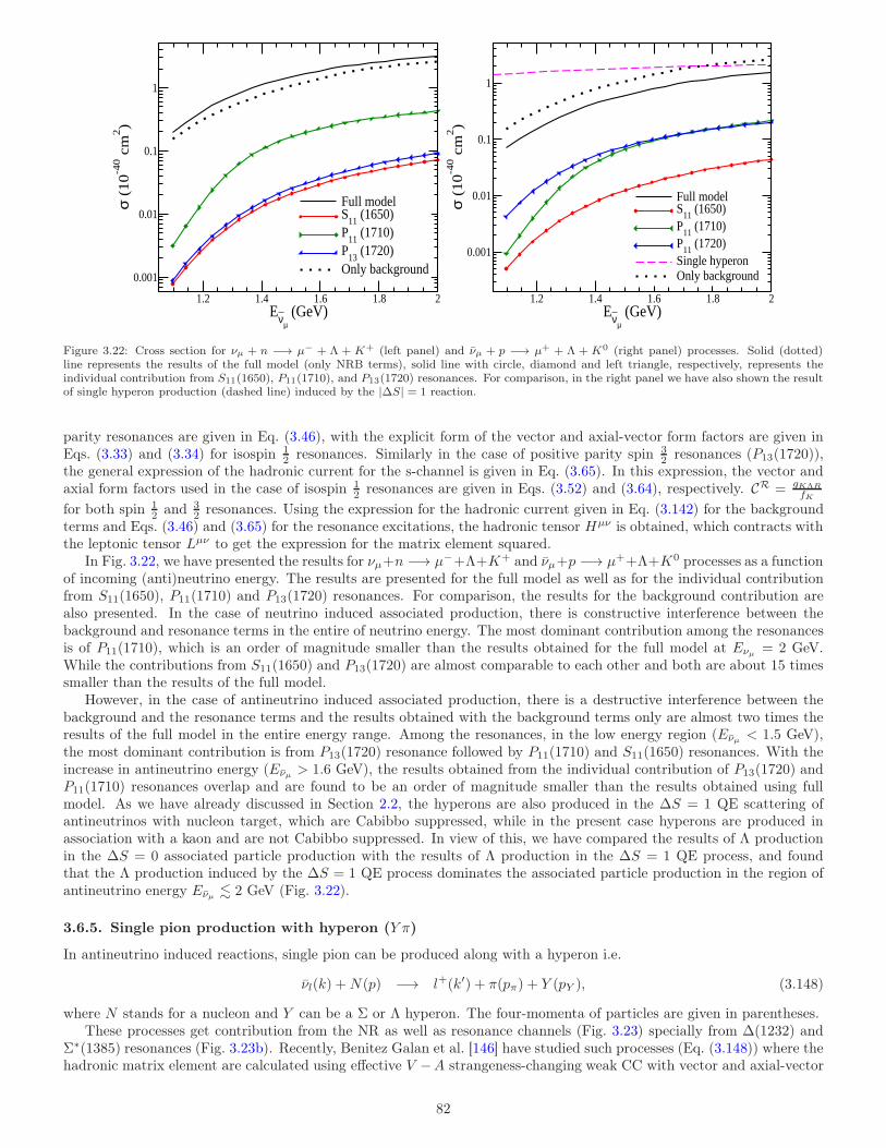
1.2 1.4 1.6 1.8 2Eνµ

(GeV)

0.001

0.01

0.1

1

σ (

10

-40 c

m2)

Full modelS

11 (1650)

P11

(1710)P

13 (1720)

Only background

1.2 1.4 1.6 1.8 2Eνµ

(GeV)

0.001

0.01

0.1

1

σ (

10

-40 c

m2)

Full modelS

11 (1650)

P11

(1710)P

11 (1720)

Single hyperonOnly background

Figure 3.22: Cross section for νµ + n −→ µ− + Λ + K+ (left panel) and νµ + p −→ µ+ + Λ + K0 (right panel) processes. Solid (dotted)line represents the results of the full model (only NRB terms), solid line with circle, diamond and left triangle, respectively, represents theindividual contribution from S11(1650), P11(1710), and P13(1720) resonances. For comparison, in the right panel we have also shown the resultof single hyperon production (dashed line) induced by the |∆S| = 1 reaction.

parity resonances are given in Eq. (3.46), with the explicit form of the vector and axial-vector form factors are given inEqs. (3.33) and (3.34) for isospin 1

2 resonances. Similarly in the case of positive parity spin 32 resonances (P13(1720)),

the general expression of the hadronic current for the s-channel is given in Eq. (3.65). In this expression, the vector andaxial form factors used in the case of isospin 1

2 resonances are given in Eqs. (3.52) and (3.64), respectively. CR = gKΛR

fK

for both spin 12 and 3

2 resonances. Using the expression for the hadronic current given in Eq. (3.142) for the backgroundterms and Eqs. (3.46) and (3.65) for the resonance excitations, the hadronic tensor Hµν is obtained, which contracts withthe leptonic tensor Lµν to get the expression for the matrix element squared.

In Fig. 3.22, we have presented the results for νµ+n −→ µ−+Λ+K+ and νµ+p −→ µ++Λ+K0 processes as a functionof incoming (anti)neutrino energy. The results are presented for the full model as well as for the individual contributionfrom S11(1650), P11(1710) and P13(1720) resonances. For comparison, the results for the background contribution arealso presented. In the case of neutrino induced associated production, there is constructive interference between thebackground and resonance terms in the entire of neutrino energy. The most dominant contribution among the resonancesis of P11(1710), which is an order of magnitude smaller than the results obtained for the full model at Eνµ = 2 GeV.While the contributions from S11(1650) and P13(1720) are almost comparable to each other and both are about 15 timessmaller than the results of the full model.

However, in the case of antineutrino induced associated production, there is a destructive interference between thebackground and the resonance terms and the results obtained with the background terms only are almost two times theresults of the full model in the entire energy range. Among the resonances, in the low energy region (Eνµ < 1.5 GeV),the most dominant contribution is from P13(1720) resonance followed by P11(1710) and S11(1650) resonances. With theincrease in antineutrino energy (Eνµ > 1.6 GeV), the results obtained from the individual contribution of P13(1720) andP11(1710) resonances overlap and are found to be an order of magnitude smaller than the results obtained using fullmodel. As we have already discussed in Section 2.2, the hyperons are also produced in the ∆S = 1 QE scattering ofantineutrinos with nucleon target, which are Cabibbo suppressed, while in the present case hyperons are produced inassociation with a kaon and are not Cabibbo suppressed. In view of this, we have compared the results of Λ productionin the ∆S = 0 associated particle production with the results of Λ production in the ∆S = 1 QE process, and foundthat the Λ production induced by the ∆S = 1 QE process dominates the associated particle production in the region ofantineutrino energy Eνµ . 2 GeV (Fig. 3.22).

3.6.5. Single pion production with hyperon (Y π)

In antineutrino induced reactions, single pion can be produced along with a hyperon i.e.

νl(k) +N(p) −→ l+(k′) + π(pπ) + Y (pY ), (3.148)

where N stands for a nucleon and Y can be a Σ or Λ hyperon. The four-momenta of particles are given in parentheses.These processes get contribution from the NR as well as resonance channels (Fig. 3.23) specially from ∆(1232) and

Σ∗(1385) resonances (Fig. 3.23b). Recently, Benitez Galan et al. [146] have studied such processes (Eq. (3.148)) where thehadronic matrix element are calculated using effective V −A strangeness-changing weak CC with vector and axial-vector

82

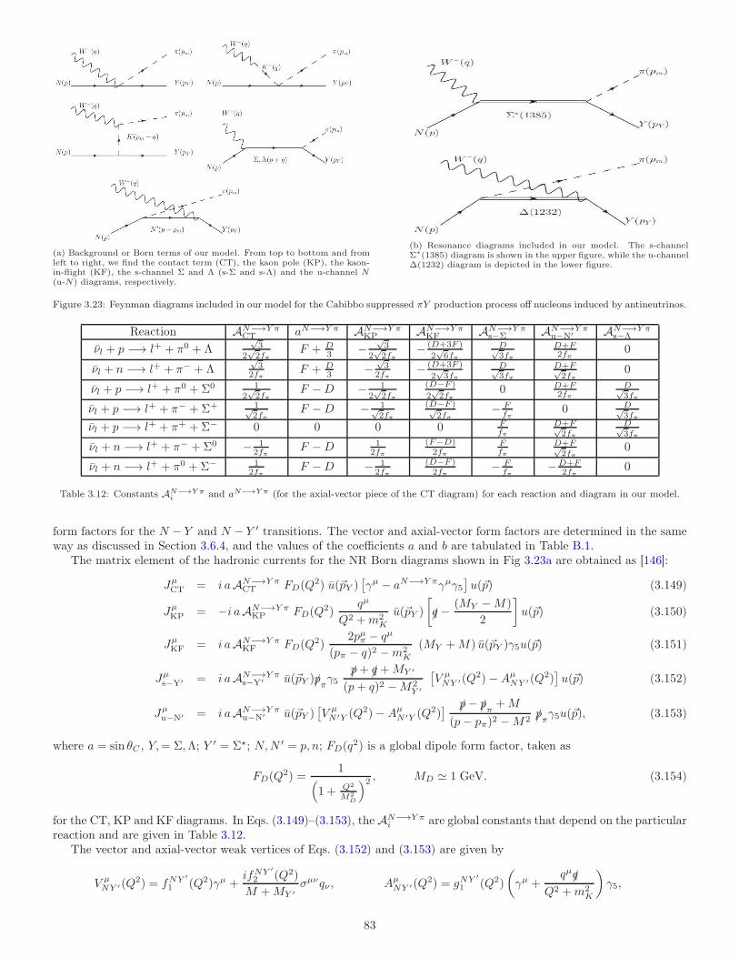
(a) Background or Born terms of our model. From top to bottom and fromleft to right, we find the contact term (CT), the kaon pole (KP), the kaon-in-flight (KF), the s-channel Σ and Λ (s-Σ and s-Λ) and the u-channel N(u-N) diagrams, respectively.

(b) Resonance diagrams included in our model. The s-channelΣ∗(1385) diagram is shown in the upper figure, while the u-channel∆(1232) diagram is depicted in the lower figure.

Figure 3.23: Feynman diagrams included in our model for the Cabibbo suppressed πY production process off nucleons induced by antineutrinos.

Reaction AN−→Y πCT aN−→Y π AN−→Y π

KP AN−→Y πKF AN−→Y π

s−Σ AN−→Y πu−N′ AN−→Y π

s−Λ

νl + p −→ l+ + π0 + Λ√3

2√2fπ

F + D3 −

√3

2√2fπ

− (D+3F )

2√6fπ

D√3fπ

D+F2fπ

0

νl + n −→ l+ + π− + Λ√3

2fπF + D

3 −√3

2fπ− (D+3F )

2√3fπ

D√3fπ

D+F√2fπ

0

νl + p −→ l+ + π0 +Σ0 12√2fπ

F −D − 12√2fπ

(D−F )

2√2fπ

0 D+F2fπ

D√3fπ

νl + p −→ l+ + π− +Σ+ 1√2fπ

F −D − 1√2fπ

(D−F )√2fπ

− Ffπ

0 D√3fπ

νl + p −→ l+ + π+ +Σ− 0 0 0 0 Ffπ

D+F√2fπ

D√3fπ

νl + n −→ l+ + π− +Σ0 − 12fπ

F −D 12fπ

(F−D)2fπ

Ffπ

D+F√2fπ

0

νl + n −→ l+ + π0 +Σ− 12fπ

F −D − 12fπ

(D−F )2fπ

− Ffπ

−D+F2fπ

0

Table 3.12: Constants AN−→Y πi and aN−→Y π (for the axial-vector piece of the CT diagram) for each reaction and diagram in our model.

form factors for the N − Y and N − Y ′ transitions. The vector and axial-vector form factors are determined in the sameway as discussed in Section 3.6.4, and the values of the coefficients a and b are tabulated in Table B.1.

The matrix element of the hadronic currents for the NR Born diagrams shown in Fig 3.23a are obtained as [146]:

JµCT = i aAN−→Y π

CT FD(Q2) u(~pY )[

γµ − aN−→Y πγµγ5]

u(~p) (3.149)

JµKP = −i aAN−→Y π

KP FD(Q2)qµ

Q2 +m2K

u(~pY )

[

/q −(MY −M)

2

]

u(~p) (3.150)

JµKF = i aAN−→Y π

KF FD(Q2)2pµπ − qµ

(pπ − q)2 −m2K

(MY +M) u(~pY )γ5u(~p) (3.151)

Jµs−Y′ = i aAN−→Y π

s−Y′ u(~pY )/pπγ5/p+ /q +MY ′

(p+ q)2 −M2Y ′

[

V µNY ′(Q

2)−AµNY ′(Q

2)]

u(~p) (3.152)

Jµu−N′ = i aAN−→Y π

u−N′ u(~pY )[

V µN ′Y (Q

2)−AµN ′Y (Q

2)] /p− /pπ +M

(p− pπ)2 −M2 /pπγ5u(~p), (3.153)

where a = sin θC , Y,= Σ,Λ; Y ′ = Σ⋆; N,N ′ = p, n; FD(q2) is a global dipole form factor, taken as

FD(Q2) =1

(

1 + Q2

M2D

)2 , MD ≃ 1 GeV. (3.154)

for the CT, KP and KF diagrams. In Eqs. (3.149)–(3.153), the AN−→Y πi are global constants that depend on the particular

reaction and are given in Table 3.12.The vector and axial-vector weak vertices of Eqs. (3.152) and (3.153) are given by

V µNY ′(Q

2) = fNY ′

1 (Q2)γµ +ifNY ′

2 (Q2)

M +MY ′

σµνqν , AµNY ′(Q

2) = gNY ′

1 (Q2)

(

γµ +qµ/q

Q2 +m2K

)

γ5,

83

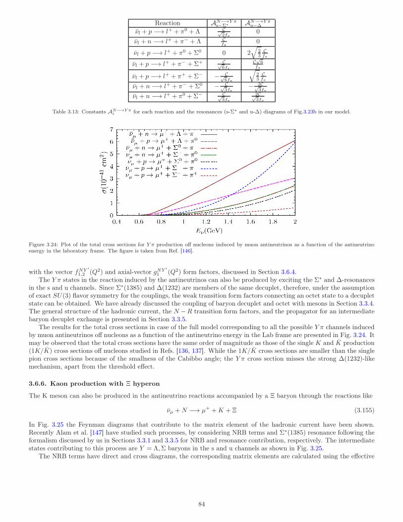
Reaction AN−→Y πs−Σ∗ AN−→Y π

u−∆

νl + p −→ l+ + π0 + Λ C√2fπ

0

νl + n −→ l+ + π− + Λ Cfπ

0

νl + p −→ l+ + π0 +Σ0 0 2√

23

Cfπ

νl + p −→ l+ + π− +Σ+ C√6fπ

C√6

fπ

νl + p −→ l+ + π+ +Σ− − C√6fπ

√

23

Cfπ

νl + n −→ l+ + π− +Σ0 − C√3fπ

− 2C√3fπ

νl + n −→ l+ + π0 +Σ− C√3fπ

2C√3fπ

Table 3.13: Constants AN−→Y πi for each reaction and the resonances (s-Σ∗ and u-∆) diagrams of Fig.3.23b in our model.

Figure 3.24: Plot of the total cross sections for Y π production off nucleons induced by muon antineutrinos as a function of the antineutrinoenergy in the laboratory frame. The figure is taken from Ref. [146].

with the vector fNY ′

1,2 (Q2) and axial-vector gNY ′

1 (Q2) form factors, discussed in Section 3.6.4.The Y π states in the reaction induced by the antineutrinos can also be produced by exciting the Σ∗ and ∆-resonances

in the s and u channels. Since Σ∗(1385) and ∆(1232) are members of the same decuplet, therefore, under the assumptionof exact SU(3) flavor symmetry for the couplings, the weak transition form factors connecting an octet state to a decupletstate can be obtained. We have already discussed the coupling of baryon decuplet and octet with mesons in Section 3.3.4.The general structure of the hadronic current, the N −R transition form factors, and the propagator for an intermediatebaryon decuplet exchange is presented in Section 3.3.5.

The results for the total cross sections in case of the full model corresponding to all the possible Y π channels inducedby muon antineutrinos off nucleons as a function of the antineutrino energy in the Lab frame are presented in Fig. 3.24. Itmay be observed that the total cross sections have the same order of magnitude as those of the single K and K production(1K/K) cross sections off nucleons studied in Refs. [136, 137]. While the 1K/K cross sections are smaller than the singlepion cross sections because of the smallness of the Cabibbo angle; the Y π cross section misses the strong ∆(1232)-likemechanism, apart from the threshold effect.

3.6.6. Kaon production with Ξ hyperon

The K meson can also be produced in the antineutrino reactions accompanied by a Ξ baryon through the reactions like

νµ +N −→ µ+ +K + Ξ (3.155)

In Fig. 3.25 the Feynman diagrams that contribute to the matrix element of the hadronic current have been shown.Recently Alam et al. [147] have studied such processes, by considering NRB terms and Σ∗(1385) resonance following theformalism discussed by us in Sections 3.3.1 and 3.3.5 for NRB and resonance contribution, respectively. The intermediatestates contributing to this process are Y = Λ,Σ baryons in the s and u channels as shown in Fig. 3.25.

The NRB terms have direct and cross diagrams, the corresponding matrix elements are calculated using the effective

84

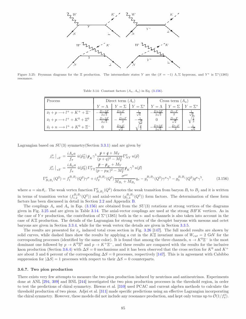
Figure 3.25: Feynman diagrams for the Ξ production. The intermediate states Y are the (S = −1) Λ,Σ hyperons, and Y ∗ is Σ∗(1385)resonance.

Table 3.14: Constant factors (As, Au) in Eq. (3.156).

Process Direct term (As) Cross term (Au)

Y = Λ Y = Σ Y = Σ∗ Y = Λ Y = Σ Y = Σ∗

νl + p −→ l+ +K+ + Ξ− −D−3F2√3

D+F2

1√6

−D+3F2√3

D−F2

1√6

νl + p −→ l+ +K0 + Ξ0 −D−3F2√3

− D+F2 − 1√

60 D−F√

2

√

23

νl + n −→ l+ +K0 + Ξ− 0 D+F√2

√

23 −D+3F

2√3

−D−F2 − 1√

6

Lagrangian based on SU(3) symmetry(Section 3.3.1) and are given by

jµcc

sY=iAsa

fπu(~p ′

Ξ) /pKγ5 /p+ /q +MY

(p+ q)2 −M2Y

ΓµNY u(~p)

jµcc

uY=iAua

fπu(~p ′

Ξ) ΓµY Ξ

/p− /pK +MY

(p− pK)2 −M2Y/pKγ

5 u(~p)

ΓµBiBj

(Q2) = fBiBj

1 (Q2)γµ + ifBiBj

2 (Q2)σµν

MBi+MBj

qν − gBiBj

1 (Q2)γµγ5 − gBiBj

3 (Q2)qµγ5, (3.156)

where a = sin θc. The weak vertex function ΓµBiBj

(Q2) denotes the weak transition from baryon Bi to Bj and it is written

in terms of transition vector (fBiBj

1,2 (Q2)) and axial-vector (gBiBj

1,3 (Q2)) form factors. The determination of these formfactors has been discussed in detail in Section 2.2 and Appendix B.

The couplings As and Au in Eqs. (3.156) are obtained from the SU(3) rotations at strong vertices of the diagramsgiven in Fig. 3.25 and are given in Table 3.14. The axial-vector couplings are used at the strong BB′K vertices. As inthe case of Y π production, the contribution of Σ∗(1385) both in the s- and u-channels is also taken into account in thecase of KΞ production. The details of the Lagrangian for strong vertex of the decuplet baryons with mesons and octetbaryons are given in Section 3.3.4, while for the weak vertex the details are given in Section 3.3.5.

The results are presented for νµ induced total cross section in Fig. 3.26 [147]. The full model results are shown bysolid curves, while dashed lines show the results by applying a cut in the KΞ invariant mass of Wcut = 2 GeV for thecorresponding processes (identified by the same color). It is found that among the three channels, n→ K0Ξ− is the mostdominant one followed by p → K0Ξ0 and p → K+Ξ−, and these results are compared with the results for the inclusivekaon production (Section 3.6.4) with ∆S = 0 mechanisms and it has been observed that the cross section for K0 and K+

are about 3 and 6 percent of the corresponding ∆S = 0 processes, respectively [147]. This is in agreement with Cabibbosuppression for |∆S| = 1 processes with respect to their ∆S = 0 counterparts.

3.6.7. Two pion production

There exists very few attempts to measure the two pion production induced by neutrinos and antineutrinos. Experimentsdone at ANL [294, 309] and BNL [244] investigated the two pion production processes in the threshold region, in orderto test the predictions of chiral symmetry. Biswas et al. [310] used PCAC and current algebra methods to calculate thethreshold production of two pions. Adjei et al. [311] made specific predictions using an effective Lagrangian incorporatingthe chiral symmetry. However, these models did not include any resonance production, and kept only terms up to O(1/f2

π).

85

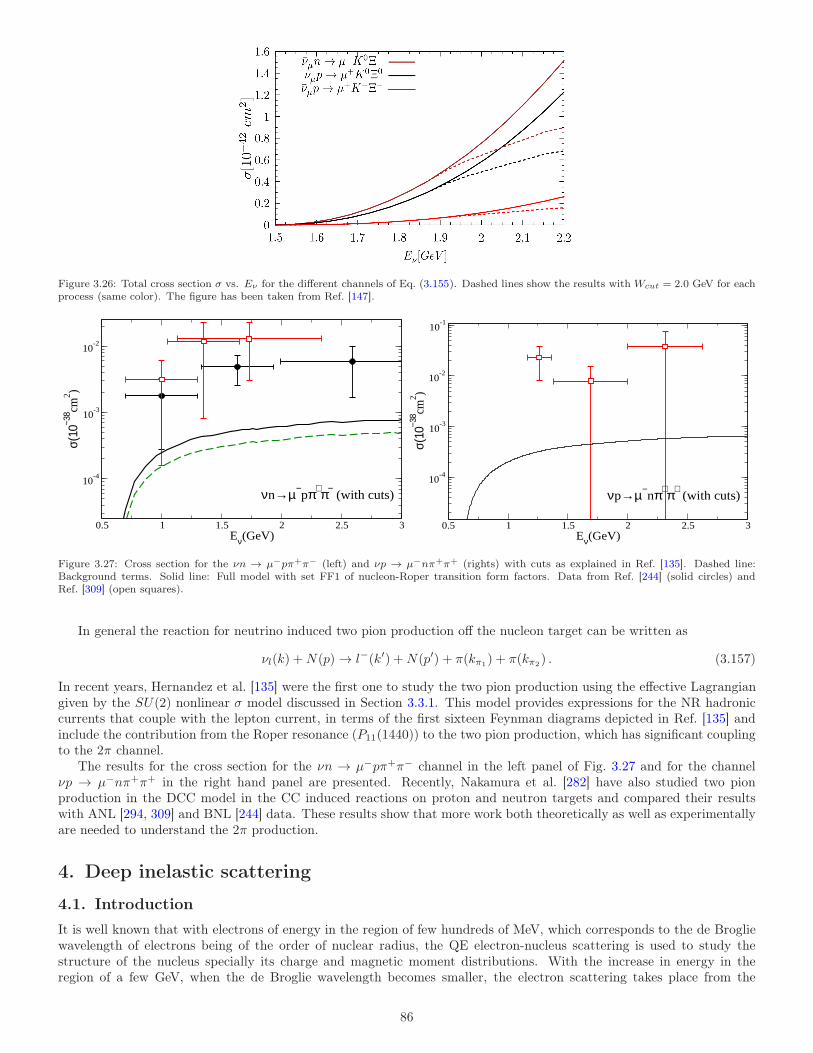
Figure 3.26: Total cross section σ vs. Eν for the different channels of Eq. (3.155). Dashed lines show the results with Wcut = 2.0 GeV for eachprocess (same color). The figure has been taken from Ref. [147].

0.5 1 1.5 2 2.5 3Eν(GeV)

10-4

10-3

10-2

σ(10

−38 cm

2 )

νn→µ−pπ+π−

(with cuts)

0.5 1 1.5 2 2.5 3Eν(GeV)

10-4

10-3

10-2

10-1

σ(10

−38 cm

2 )

νp→µ−nπ+π+

(with cuts)

Figure 3.27: Cross section for the νn → µ−pπ+π− (left) and νp → µ−nπ+π+ (rights) with cuts as explained in Ref. [135]. Dashed line:Background terms. Solid line: Full model with set FF1 of nucleon-Roper transition form factors. Data from Ref. [244] (solid circles) andRef. [309] (open squares).

In general the reaction for neutrino induced two pion production off the nucleon target can be written as

νl(k) +N(p)→ l−(k′) +N(p′) + π(kπ1) + π(kπ2) . (3.157)

In recent years, Hernandez et al. [135] were the first one to study the two pion production using the effective Lagrangiangiven by the SU(2) nonlinear σ model discussed in Section 3.3.1. This model provides expressions for the NR hadroniccurrents that couple with the lepton current, in terms of the first sixteen Feynman diagrams depicted in Ref. [135] andinclude the contribution from the Roper resonance (P11(1440)) to the two pion production, which has significant couplingto the 2π channel.

The results for the cross section for the νn → µ−pπ+π− channel in the left panel of Fig. 3.27 and for the channelνp → µ−nπ+π+ in the right hand panel are presented. Recently, Nakamura et al. [282] have also studied two pionproduction in the DCC model in the CC induced reactions on proton and neutron targets and compared their resultswith ANL [294, 309] and BNL [244] data. These results show that more work both theoretically as well as experimentallyare needed to understand the 2π production.

4. Deep inelastic scattering

4.1. Introduction

It is well known that with electrons of energy in the region of few hundreds of MeV, which corresponds to the de Brogliewavelength of electrons being of the order of nuclear radius, the QE electron-nucleus scattering is used to study thestructure of the nucleus specially its charge and magnetic moment distributions. With the increase in energy in theregion of a few GeV, when the de Broglie wavelength becomes smaller, the electron scattering takes place from the

86

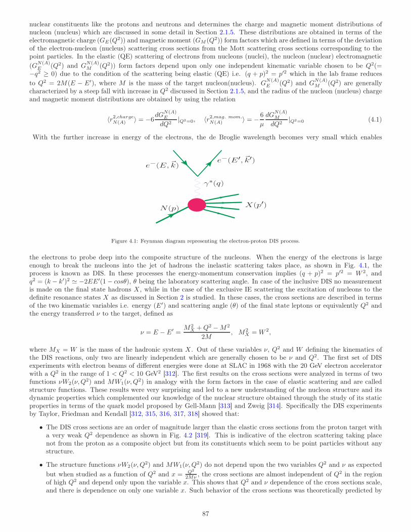
nuclear constituents like the protons and neutrons and determines the charge and magnetic moment distributions ofnucleon (nucleus) which are discussed in some detail in Section 2.1.5. These distributions are obtained in terms of theelectromagnetic charge (GE(Q

2)) and magnetic moment (GM (Q2)) form factors which are defined in terms of the deviationof the electron-nucleon (nucleus) scattering cross sections from the Mott scattering cross sections corresponding to thepoint particles. In the elastic (QE) scattering of electrons from nucleons (nuclei), the nucleon (nuclear) electromagnetic

(GN(A)E (Q2) and G

N(A)M (Q2)) form factors depend upon only one independent kinematic variable chosen to be Q2(=

−q2 ≥ 0) due to the condition of the scattering being elastic (QE) i.e. (q + p)2 = p′2 which in the lab frame reduces

to Q2 = 2M(E − E′), where M is the mass of the target nucleon(nucleus). GN(A)E (Q2) and G

N(A)M (Q2) are generally

characterized by a steep fall with increase in Q2 discussed in Section 2.1.5, and the radius of the nucleon (nucleus) chargeand magnetic moment distributions are obtained by using the relation

〈r2,chargeN(A) 〉 = −6dGN(A)E

dQ2|Q2=0, 〈r2,mag. mom.

N(A) 〉 = − 6

µ

dGN(A)M

dQ2|Q2=0 (4.1)

With the further increase in energy of the electrons, the de Broglie wavelength becomes very small which enables

e−(E,~k)e−(E′, ~k′)

γ∗(q)

N (p) X(p′)

Figure 4.1: Feynman diagram representing the electron-proton DIS process.

the electrons to probe deep into the composite structure of the nucleons. When the energy of the electrons is largeenough to break the nucleons into the jet of hadrons the inelastic scattering takes place, as shown in Fig. 4.1, theprocess is known as DIS. In these processes the energy-momentum conservation implies (q + p)2 = p′2 = W 2, andq2 = (k − k′)2 ≃ −2EE′(1− cosθ), θ being the laboratory scattering angle. In case of the inclusive DIS no measurementis made on the final state hadrons X , while in the case of the exclusive IE scattering the excitation of nucleons to thedefinite resonance states X as discussed in Section 2 is studied. In these cases, the cross sections are described in termsof the two kinematic variables i.e. energy (E′) and scattering angle (θ) of the final state leptons or equivalently Q2 andthe energy transferred ν to the target, defined as

ν = E − E′ =M2

X +Q2 −M2

2M, M2

X =W 2,

where MX = W is the mass of the hadronic system X . Out of these variables ν, Q2 and W defining the kinematics ofthe DIS reactions, only two are linearly independent which are generally chosen to be ν and Q2. The first set of DISexperiments with electron beams of different energies were done at SLAC in 1968 with the 20 GeV electron acceleratorwith a Q2 in the range of 1 < Q2 < 10 GeV2 [312]. The first results on the cross sections were analyzed in terms of twofunctions νW2(ν,Q

2) and MW1(ν,Q2) in analogy with the form factors in the case of elastic scattering and are called

structure functions. These results were very surprising and led to a new understanding of the nucleon structure and itsdynamic properties which complemented our knowledge of the nuclear structure obtained through the study of its staticproperties in terms of the quark model proposed by Gell-Mann [313] and Zweig [314]. Specifically the DIS experimentsby Taylor, Friedman and Kendall [312, 315, 316, 317, 318] showed that:

• The DIS cross sections are an order of magnitude larger than the elastic cross sections from the proton target witha very weak Q2 dependence as shown in Fig. 4.2 [319]. This is indicative of the electron scattering taking placenot from the proton as a composite object but from its constituents which seem to be point particles without anystructure.

• The structure functions νW2(ν,Q2) and MW1(ν,Q

2) do not depend upon the two variables Q2 and ν as expected

but when studied as a function of Q2 and x = Q2

2Mν , the cross sections are almost independent of Q2 in the regionof high Q2 and depend only upon the variable x. This shows that Q2 and ν dependence of the cross sections scale,and there is dependence on only one variable x. Such behavior of the cross sections was theoretically predicted by

87

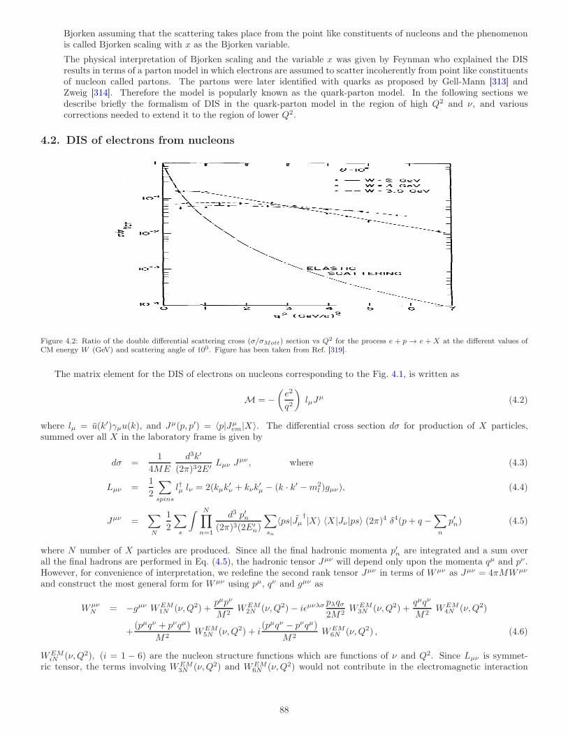
Bjorken assuming that the scattering takes place from the point like constituents of nucleons and the phenomenonis called Bjorken scaling with x as the Bjorken variable.

The physical interpretation of Bjorken scaling and the variable x was given by Feynman who explained the DISresults in terms of a parton model in which electrons are assumed to scatter incoherently from point like constituentsof nucleon called partons. The partons were later identified with quarks as proposed by Gell-Mann [313] andZweig [314]. Therefore the model is popularly known as the quark-parton model. In the following sections wedescribe briefly the formalism of DIS in the quark-parton model in the region of high Q2 and ν, and variouscorrections needed to extend it to the region of lower Q2.

4.2. DIS of electrons from nucleons

Figure 4.2: Ratio of the double differential scattering cross (σ/σMott) section vs Q2 for the process e + p → e +X at the different values ofCM energy W (GeV) and scattering angle of 100. Figure has been taken from Ref. [319].

The matrix element for the DIS of electrons on nucleons corresponding to the Fig. 4.1, is written as

M = −(

e2

q2

)

lµJµ (4.2)

where lµ = u(k′)γµu(k), and Jµ(p, p′) = 〈p|Jµem|X〉. The differential cross section dσ for production of X particles,

summed over all X in the laboratory frame is given by

dσ =1

4ME

d3k′

(2π)32E′ Lµν Jµν , where (4.3)

Lµν =1

2

∑

spins

l†µ lν = 2(kµk′ν + kνk

′µ − (k · k′ −m2

l )gµν), (4.4)

Jµν =∑

N

1

2

∑

s

∫ N∏

n=1

d3 p′n(2π)3(2E′

n)

∑

sn

〈ps|Jµ†|X〉 〈X |Jν |ps〉 (2π)4 δ4(p+ q −

∑

n

p′n) (4.5)

where N number of X particles are produced. Since all the final hadronic momenta p′n are integrated and a sum overall the final hadrons are performed in Eq. (4.5), the hadronic tensor Jµν will depend only upon the momenta qµ and pν .However, for convenience of interpretation, we redefine the second rank tensor Jµν in terms of Wµν as Jµν = 4πMWµν

and construct the most general form for Wµν using pµ, qν and gµν as

WµνN = −gµν WEM

1N (ν,Q2) +pµpν

M2WEM

2N (ν,Q2)− iǫµνλσ pλqσ2M2

WEM3N (ν,Q2) +

qµqν

M2WEM

4N (ν,Q2)

+(pµqν + pνqµ)

M2WEM

5N (ν,Q2) + i(pµqν − pνqµ)

M2WEM

6N (ν,Q2) , (4.6)

WEMiN (ν,Q2), (i = 1 − 6) are the nucleon structure functions which are functions of ν and Q2. Since Lµν is symmet-

ric tensor, the terms involving WEM3N (ν,Q2) and WEM

6N (ν,Q2) would not contribute in the electromagnetic interaction

88

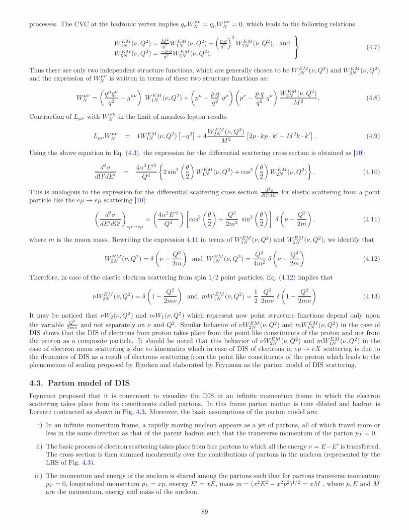
processes. The CVC at the hadronic vertex implies qνWµνN = qµW

µνN = 0, which leads to the following relations

WEM4N (ν,Q2) = M2

q2 WEM1N (ν,Q2) +

(

p·qq2

)2

WEM2N (ν,Q2), and

WEM5N (ν,Q2) = −p·q

q2 WEM2N (ν,Q2).

(4.7)

Thus there are only two independent structure functions, which are generally chosen to be WEM1N (ν,Q2) and WEM

2N (ν,Q2)and the expression of Wµν

N is written in terms of these two structure functions as:

WµνN =

(

qµqν

q2− gµν

)

WEM1N (ν,Q2) +

(

pµ − p.q

q2qµ)(

pν − p.q

q2qν)

WEM2N (ν,Q2)

M2. (4.8)

Contraction of Lµν with WµνN in the limit of massless lepton results

LµνWµνN = 4WEM

1N (ν,Q2)[

−q2]

+ 4WEM

2N (ν,Q2)

M2

[

2p · kp · k′ −M2k · k′]

. (4.9)

Using the above equation in Eq. (4.3), the expression for the differential scattering cross section is obtained as [10]:

d2σ

dΩ′dE′ =4α2E′2

Q4

2 sin2(

θ

2

)

WEM1N (ν,Q2) + cos2

(

θ

2

)

WEM2N (ν,Q2)

. (4.10)

This is analogous to the expression for the differential scattering cross section d2σdΩ′dE′ for elastic scattering from a point

particle like the eµ→ eµ scattering [10]:

(

d2σ

dE′dΩ′

)

eµ→eµ

=

(

4α2E′2

Q4

)[

cos2(

θ

2

)

+Q2

2m2sin2

(

θ

2

)]

δ

(

ν − Q2

2m

)

, (4.11)

where m is the muon mass. Rewriting the expression 4.11 in terms of WEM1N (ν,Q2) and WEM

2N (ν,Q2), we identify that

WEM2N (ν,Q2) = δ

(

ν − Q2

2m

)

and WEM1N (ν,Q2) =

Q2

4m2δ

(

ν − Q2

2m

)

(4.12)

Therefore, in case of the elastic electron scattering from spin 1/2 point particles, Eq. (4.12) implies that

νWEM2N (ν,Q2) = δ

(

1− Q2

2mν

)

and mWEM1N (ν,Q2) =

1

2

Q2

2mνδ

(

1− Q2

2mν

)

(4.13)

It may be noticed that νW2(ν,Q2) and mW1(ν,Q

2) which represent now point structure functions depend only upon

the variable Q2

2mν and not separately on ν and Q2. Similar behavior of νWEM2N (ν,Q2) and mWEM

1N (ν,Q2) in the case ofDIS shows that the DIS of electrons from proton takes place from the point like constituents of the proton and not fromthe proton as a composite particle. It should be noted that this behavior of νWEM

2N (ν,Q2) and mWEM1N (ν,Q2) in the

case of electron muon scattering is due to kinematics which in case of DIS of electrons in ep → eX scattering is due tothe dynamics of DIS as a result of electrons scattering from the point like constituents of the proton which leads to thephenomenon of scaling proposed by Bjorken and elaborated by Feynman as the parton model of DIS scattering.

4.3. Parton model of DIS

Feynman proposed that it is convenient to visualize the DIS in an infinite momentum frame in which the electronscattering takes place from its constituents called partons. In this frame parton motion is time dilated and hadron isLorentz contracted as shown in Fig. 4.3. Moreover, the basic assumptions of the parton model are:

i) In an infinite momentum frame, a rapidly moving nucleon appears as a jet of partons, all of which travel more orless in the same direction as that of the parent hadron such that the transverse momentum of the parton pT = 0.

ii) The basic process of electron scattering takes place from free partons to which all the energy ν = E−E′ is transferred.The cross section is then summed incoherently over the contributions of partons in the nucleon (represented by theLHS of Fig. 4.3).

iii) The momentum and energy of the nucleon is shared among the partons such that for partons transverse momentumpT = 0, longitudinal momentum pL = xp, energy E′ = xE, mass m = (x2E2 − x2p2)1/2 = xM , where p,E and Mare the momentum, energy and mass of the nucleon.

89

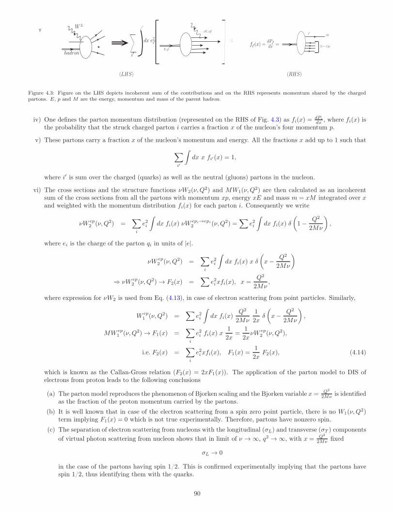
E, ~p

xE, x~p

i′

dx e2i′

W±

hadron

fi′(x) =dPi′dx = (1− x)p

xpi′

;

(LHS) (RHS)

Figure 4.3: Figure on the LHS depicts incoherent sum of the contributions and on the RHS represents momentum shared by the chargedpartons. E, p and M are the energy, momentum and mass of the parent hadron.

iv) One defines the parton momentum distribution (represented on the RHS of Fig. 4.3) as fi(x) =dPi

dx , where fi(x) isthe probability that the struck charged parton i carries a fraction x of the nucleon’s four momentum p.

v) These partons carry a fraction x of the nucleon’s momentum and energy. All the fractions x add up to 1 such that

∑

i′

∫

dx x fi′(x) = 1,

where i′ is sum over the charged (quarks) as well as the neutral (gluons) partons in the nucleon.

vi) The cross sections and the structure functions νW2(ν,Q2) and MW1(ν,Q

2) are then calculated as an incoherentsum of the cross sections from all the partons with momentum xp, energy xE and mass m = xM integrated over xand weighted with the momentum distribution fi(x) for each parton i. Consequently we write

νW ep2 (ν,Q2) =

∑

i

e2i

∫

dx fi(x) νWepi→epi

2 (ν,Q2) =∑

e2i

∫

dx fi(x) δ

(

1− Q2

2Mν

)

,

where ei is the charge of the parton qi in units of |e|.

νW ep2 (ν,Q2) =

∑

i

e2i

∫

dx fi(x) x δ

(

x− Q2

2Mν

)

⇒ νW ep2 (ν,Q2)→ F2(x) =

∑

e2ixfi(x), x =Q2

2Mν,

where expression for νW2 is used from Eq. (4.13), in case of electron scattering from point particles. Similarly,

W ep1 (ν,Q2) =

∑

e2i

∫

dx fi(x)Q2

2Mν

1

2xδ

(

x− Q2

2Mν

)

,

MW ep1 (ν,Q2)→ F1(x) =

∑

i

e2i fi(x) x1

2x=

1

2xνW ep

2 (ν,Q2),

i.e. F2(x) =∑

i

e2ixfi(x), F1(x) =1

2xF2(x), (4.14)

which is known as the Callan-Gross relation (F2(x) = 2xF1(x)). The application of the parton model to DIS ofelectrons from proton leads to the following conclusions

(a) The parton model reproduces the phenomenon of Bjorken scaling and the Bjorken variable x = Q2

2Mν is identifiedas the fraction of the proton momentum carried by the partons.

(b) It is well known that in case of the electron scattering from a spin zero point particle, there is no W1(ν,Q2)

term implying F1(x) = 0 which is not true experimentally. Therefore, partons have nonzero spin.

(c) The separation of electron scattering from nucleons with the longitudinal (σL) and transverse (σT ) components

of virtual photon scattering from nucleon shows that in limit of ν →∞, q2 →∞, with x = Q2

2Mν fixed

σL → 0

in the case of the partons having spin 1/2. This is confirmed experimentally implying that the partons havespin 1/2, thus identifying them with the quarks.

90

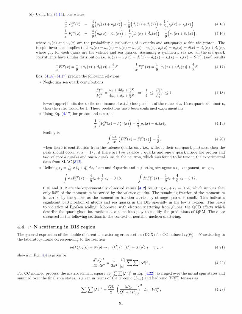
(d) Using Eq. (4.14), one writes

1

xF ep2 (x) =

4

9

(

up(x) + up(x))

+1

9

(

dp(x) + dp(x))

+1

9

(

sp(x) + sp(x))

, (4.15)

1

xF en2 (x) =

4

9

(

un(x) + un(x))

+1

9

(

dn(x) + dn(x))

+1

9

(

sn(x) + sn(x))

, (4.16)

where up(x) and up(x) are the probability distributions of u quarks and antiquarks within the proton. Theisospin invariance implies that up(x) = dn(x) = u(x) = uv(x) + us(x), dp(x) = un(x) = d(x) = dv(x) + ds(x),where qv,s for each quark are the valence and sea quarks. Assuming a symmetric sea i.e. all the sea quarkconstituents have similar distribution i.e. us(x) = us(x) = ds(x) = ds(x) = ss(x) = ss(x) = S(x), (say) results

1

xF ep2 (x) =

1

9[4uv(x) + dv(x)] +

4

3S,

1

xF en2 (x) =

1

9[uv(x) + 4dv(x)] +

4

3S (4.17)

Eqs. (4.15)–(4.17) predict the following relations:

∗ Neglecting sea quark contributions

F en2

F ep2

=uv + 4dv +

43S

4uv + dv +43S

⇒ 1

4≤ F en

2

F ep2

≤ 4. (4.18)

lower (upper) limits due to the dominance of uv(dv) independent of the value of x. If sea quarks dominates,then the ratio would be 1. These predictions have been confirmed experimentally.

∗ Using Eq. (4.17) for proton and neutron

1

x

(

F ep2 (x) − F en

2 (x))

=1

3[uv(x) − dv(x)], (4.19)

leading to∫

dx

x

(

F ep2 (x) − F en

2 (x))

=1

3, (4.20)

when there is contribution from the valence quarks only i.e., without their sea quark partners, then thepeak should occur at x = 1/3, if there are two valence u quarks and one d quark inside the proton andtwo valence d quarks and one u quark inside the neutron, which was found to be true in the experimentaldata from SLAC [312].

∗ Defining ǫq =∫ 1

0x (q + q) dx, for u and d quarks and neglecting strangeness ǫs component, we get,

∫

dxF ep2 (x) =

4

9ǫu +

1

9ǫd = 0.18,

∫

dxF en2 (x) =

1

9ǫu +

4

9ǫd = 0.12,

0.18 and 0.12 are the experimentally observed values [312] resulting ǫu + ǫd = 0.54, which implies thatonly 54% of the momentum is carried by the valence quarks. The remaining fraction of the momentumis carried by the gluons as the momentum fraction carried by strange quarks is small. This indicatessignificant participation of gluons and sea quarks in the DIS specially in the low x region. This leadsto violation of Bjorken scaling. Moreover, with electron scattering from gluons, the QCD effects whichdescribe the quark-gluon interactions also come into play to modify the predictions of QPM. These arediscussed in the following sections in the context of neutrino-nucleon scattering.

4.4. ν–N scattering in DIS region

The general expression of the double differential scattering cross section (DCX) for CC induced νl(νl)−N scattering inthe laboratory frame corresponding to the reaction:

νl(k)/νl(k) +N(p)→ l−(k′)/l+(k′) +X(p′); l = e, µ, τ, (4.21)

shown in Fig. 4.4 is given by

d2σWIN

dΩ′dE′ =1

2π2

|~k′||~k|

∑∑

|M|2 , (4.22)

For CC induced process, the matrix element square i.e.∑∑ |M|2 in Eq. (4.22), averaged over the initial spin states and

summed over the final spin states, is given in terms of the leptonic (Lµν) and hadronic (WµνN ) tensors as

∑∑

|M|2 =G2

F

2

(

M2W

Q2 +M2W

)2

Lµν WµνN , (4.23)

91

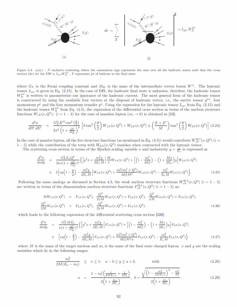
X

2

dσ ∼ ∼ Lµν WµνN

X(p′)

W+/W

− (q)

N(p)

νl/νl (k)

l−/l+ (k

′ )

X(p′)

W+ /W

− (q)

N(p)

νl/νl(k)l− /l

+ (k′ )

(a) (b)

Figure 4.4: νl(νl) − N inclusive scattering where the summation sign represents the sum over all the hadronic states such that the crosssection (dσ) for the DIS ∝ LµνW

µνN . X represents jet of hadrons in the final state.

where GF is the Fermi coupling constant and MW is the mass of the intermediate vector boson W±. The leptonictensor Lµν is given in Eq. (2.15). In the case of DIS, the hadronic final state is unknown, therefore, the hadronic tensorWµν

N is written to parameterize our ignorance of the hadronic current. The most general form of the hadronic tensoris constructed by using the available four vectors at the disposal of hadronic vertex, i.e., the metric tensor gµν , fourmomentum pµ and the four momentum transfer qµ. Using the expression for the leptonic tensor Lµν from Eq. (2.15) andthe hadronic tensor Wµν

N from Eq. (4.5), the expression of the differential cross section in terms of the nucleon structurefunctions WiN (ν,Q2); (i = 1− 3) for the case of massless lepton (ml → 0) is obtained as [10]:

d2σ

dΩ′ dE′ =G2

FE′2 cos2

(

θ2

)

2π2(

1 + Q2

M2W

)2

[

2 tan2(

θ

2

)

W1N (ν,Q2) +W2N (ν,Q2)±(

E + E′

M

)

tan2(

θ

2

)

W3N (ν,Q2)]

(4.24)

In the case of massive lepton, all the five structure functions (as mentioned in Eq. (4.5)) would contributeWWIiN (ν,Q2) (i =

1− 5) while the contribution of the term with W6N (ν,Q2) vanishes when contracted with the leptonic tensor.The scattering cross section in terms of the Bjorken scaling variable x and inelasticity y = ν

Eνis expressed as

d2σ

dxdy=

G2FEνQ

2

2πx(1 + Q2

M2W

)2

[

y2x+

m2l y

2EνM

]

M

νW1N (x,Q2) +

[(

1− m2l

4E2ν

)

−(

1 +Mx

2Eν

)

y]

W2N (x,Q2)

± 2[

xy(

1− y

2

)

− m2l y

4EνM

]

W3N(x,Q2) +m2

l (m2l +Q2)

4E2νM

2W4N (x,Q2)− m2

l

EνMW5N (x,Q2)

. (4.25)

Following the same analogy as discussed in Section 4.3, the weak nucleon structure functions WWIiN (ν,Q2) (i = 1 − 5)

are written in terms of the dimensionless nucleon structure functions FWIiN (x,Q2) (i = 1− 5) as:

MW1N (ν,Q2) = F1N (x,Q2),Q2

2xMW2N(ν,Q2) = F2N (x,Q2),

Q2

xMW3N(ν,Q2) = F3N (x,Q2),

Q2

2MW4N (ν,Q2) = F4N (x,Q2),

Q2

2xMW5N(ν,Q2) = F5N (x,Q2). (4.26)

which leads to the following expression of the differential scattering cross section [320]:

d2σ

dxdy=

G2FMEν

π(1 + Q2

M2W

)2

[

y2x+

m2l y

2EνM

]

F1N (x,Q2) +[(

1− m2l

4E2ν

)

−(

1 +Mx

2Eν

)

y]

F2N (x,Q2)

±[

xy(

1− y

2

)

− m2l y

4EνM

]

F3N (x,Q2) +m2

l (m2l +Q2)

4E2νM

2xF4N (x,Q2)− m2

l

EνMF5N (x,Q2)

. (4.27)

where M is the mass of the target nucleon and ml is the mass of the final state charged lepton. x and y are the scalingvariables which lie in the following ranges:

m2l

2M(Eν −ml)≤ x ≤ 1; a− b ≤ y ≤ a+ b, with (4.28)

a =1−m2

l

(

12MEνx

+ 12E2

ν

)

2(

1 + Mx2Eν

) , b =

√

(

1− m2l

2MEνx

)2

− m2l

E2ν

2(

1 + Mx2Eν

) . (4.29)

92

In general, the dimensionless nucleon structure functions are derived in the quark-parton model assuming Bjorken scalingand are functions of only one variable x. In this model, these structure functions obey Callan-Gross [321] and Albright-Jarlskog [322] relations, respectively given by

F1(x) =F2(x)

2x; F5(x) =

F2(x)

2x,

At the leading order of perturbative QCD, the structure functions are derived in terms of the parton distribution functionsqi(x) and qi(x) as:

F2(x) =∑

i

x[qi(x) + qi(x)] ; xF3(x) =∑

i

x[qi(x) − qi(x)] ; F4(x) = 0. (4.30)

Generally, the proton (F p1,2(x)) and the neutron (Fn

1,2(x)) structure functions are obtained in the four flavor quark schemeassuming that the heavy quark flavors (b and t) do not contribute as they are massive in comparison to the nucleon’smass (M << mb or mt) with the following result:

F νlp2 (x) = 2x[d(x) + s(x) + u(x) + c(x)] , F νlp

2 (x) = 2x[u(x) + c(x) + d(x) + s(x)]

F νln2 (x) = 2x[u(x) + s(x) + d(x) + c(x)] , F νln

2 (x) = 2x[d(x) + c(x) + u(x) + s(x)]

xF νlp3 (x) = 2x[d(x) + s(x) − u(x) − c(x)] , xF νlp

3 (x) = 2x[u(x) + c(x)− d(x) − s(x)]xF νln

3 (x) = 2x[u(x) + s(x)− d(x) − c(x)] , xF νln3 (x) = 2x[d(x) + c(x) − u(x) − s(x)].

In the above expressions, xu(x) represents the probability of finding an up quark with the target nucleon’s momentumfraction x and similarly for other quark flavors. These probability distributions are also known as parton distributionfunctions (PDFs). The parton distribution functions for the nucleon have phenomenologically been determined by var-ious groups and they are known in the literature by the acronyms MRST [323], GRV [324], GJR [325], MSTW [326],ABMP [327], ZEUS [328], HERAPDF [329], NNPDF [330], CTEQ [331], CTEQ-Jefferson Lab (CJ) [332], MMHT [333],etc.

For an isoscalar nucleon target, the structure functions are defined for nucleon FiN as:

FiN =Fip + Fin

2. (i = 1− 5) (4.31)

The neutrino scattering experiments performed at CERN using heavy liquid bubble chamber Gargamelle also providedsome conclusive evidence in support of the quark-parton model [334]:

• For an isoscalar target the ratio of the F2(x) structure functions in electron and neutrino scattering in the partonmodel depends only on the quark charges, i.e.,

12

∫

[F νp2 (x) + F νn

2 (x)]dx12

∫

[F ep2 (x) + F en

2 (x)]dx=

2

e2u + e2d=

18

5, (4.32)

where the strange quark contribution has been neglected, and eu and ed are respectively the electric charges of the uand d quarks. The observed value for this ratio was 3.4±0.7 [335]. This test provided the most convincing evidencethat the nucleons are made up of quarks which have fractional electric charge as real dynamical entities.

• In the quark-parton model for the point-like constituents it was observed that the total (anti)neutrino scatteringcross sections is proportional to the energy in CM frame which was verified by Gargamelle collaboration [335].

• The Gross-Llewellyn-Smith sum rule [336] in the quark-parton model states that:

∫ 1

0

F3N (x)dx =

∫ 1

0

[u(x)− u(x) + d(x) − d(x)]dx = 3. (4.33)

which was reported by the Gargamelle collaboration to be 3.2± 0.6 [335].

In the lowest order of perturbative QCD, the partons are treated as free, noninteracting constituents of nucleon, butthe partons present inside the nucleon may interact among themselves via the gluon exchange which can be describedusing QCD. The incorporation of contribution from gluon emission induces the Q2 dependence of the nucleon structurefunctions, leading to the violation of Bjorken scaling. TheQ2 evolution of structure functions is determined by the DGLAPevolution equation [337]. In Fig. 4.5, the experimental results for the nucleon structure functions from several electronscattering experiments [338, 339, 340, 341, 342], and neutrino scattering experiments like CCFR [343], CDHSW [344],etc. are presented in a wide range of x and Q2. One may notice from the figure that with the increase in x and Q2, thestructure functions decreases, while for lower x and Q2 there is a rise. This behavior of structure functions show scalingbreakdown which may be observed from Fig. 4.5. In the next section, we discuss some of the experimental results for thetotal cross section from various neutrino scattering experiments.

93

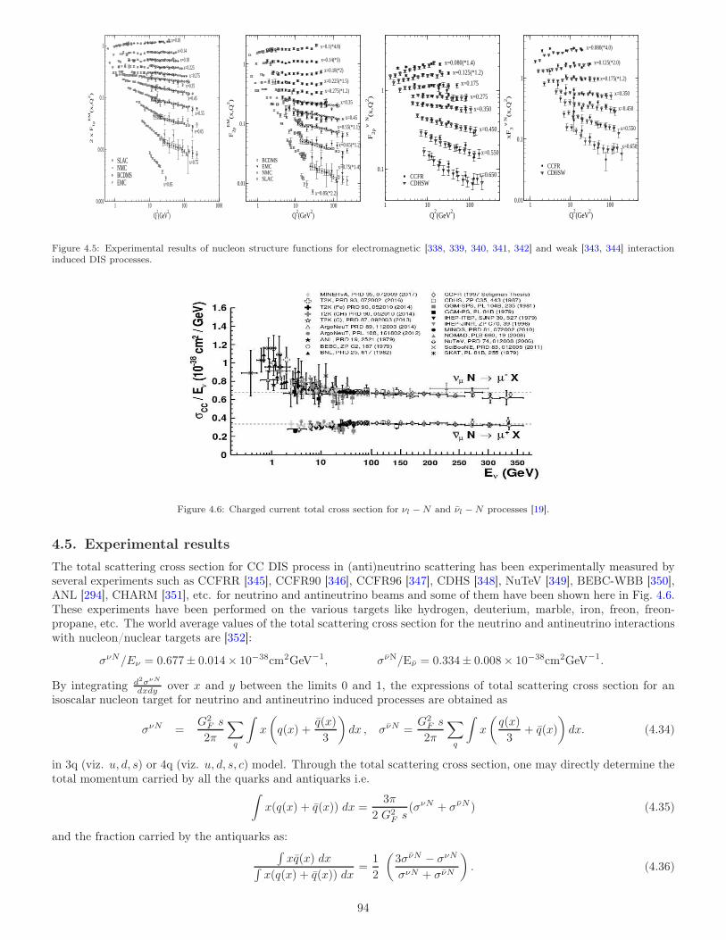
1 10 100 1000

Q2(GeV

2)

0.001

0.01

0.1

1

2 x

F1

p

EM

(x

,Q2)

SLACNMCBCDMSEMC

x=0.35

x=0.45

x=0.55

x=0.65

x=0.75

x=0.85

x=0.275x=0.225

x=0.10

x=0.14

x=0.18

1 10 100

Q2(GeV

2)

0.01

0.1

1

F2p

EM

(x,Q

2)

BCDMSEMCNMCSLAC

x=0.1(*4.8)

x=0.14(*3)

x=0.18(*2)

x=0.225(*1.5)

x=0.275(*1.2)

x=0.35

x=0.45

x=0.55(*1.1)

x=0.65(*1.2)

x=0.75(*1.4)

x=0.85(*2.2)

1 10 100

Q2(GeV

2)

0.1

1

F2

p

ν N

(x,Q

2)

CCFRCDHSW

x=0.650

x=0.550

x=0.450

x=0.350

x=0.275

x=0.175

x=0.080(*1.4)

x=0.125(*1.2)

1 10 100

Q2(GeV

2)

0.01

0.1

1

xF

3

ν N

(x,Q

2)

CCFRCDHSW

x=0.650

x=0.550

x=0.450

x=0.350

x=0.175(*1.2)

x=0.125(*2.0)

x=0.080(*4.0)

Figure 4.5: Experimental results of nucleon structure functions for electromagnetic [338, 339, 340, 341, 342] and weak [343, 344] interactioninduced DIS processes.

Figure 4.6: Charged current total cross section for νl −N and νl −N processes [19].

4.5. Experimental results

The total scattering cross section for CC DIS process in (anti)neutrino scattering has been experimentally measured byseveral experiments such as CCFRR [345], CCFR90 [346], CCFR96 [347], CDHS [348], NuTeV [349], BEBC-WBB [350],ANL [294], CHARM [351], etc. for neutrino and antineutrino beams and some of them have been shown here in Fig. 4.6.These experiments have been performed on the various targets like hydrogen, deuterium, marble, iron, freon, freon-propane, etc. The world average values of the total scattering cross section for the neutrino and antineutrino interactionswith nucleon/nuclear targets are [352]:

σνN/Eν = 0.677± 0.014× 10−38cm2GeV−1, σνN/Eν = 0.334± 0.008× 10−38cm2GeV−1.

By integrating d2σνN

dxdy over x and y between the limits 0 and 1, the expressions of total scattering cross section for anisoscalar nucleon target for neutrino and antineutrino induced processes are obtained as

σνN =G2

F s

2π

∑

q

∫

x

(

q(x) +q(x)

3

)

dx , σνN =G2

F s

2π

∑

q

∫

x

(

q(x)

3+ q(x)

)

dx. (4.34)

in 3q (viz. u, d, s) or 4q (viz. u, d, s, c) model. Through the total scattering cross section, one may directly determine thetotal momentum carried by all the quarks and antiquarks i.e.

∫

x(q(x) + q(x)) dx =3π

2 G2F s

(σνN + σνN ) (4.35)

and the fraction carried by the antiquarks as:∫

xq(x) dx∫

x(q(x) + q(x)) dx=

1

2

(

3σνN − σνN

σνN + σνN

)

. (4.36)

94

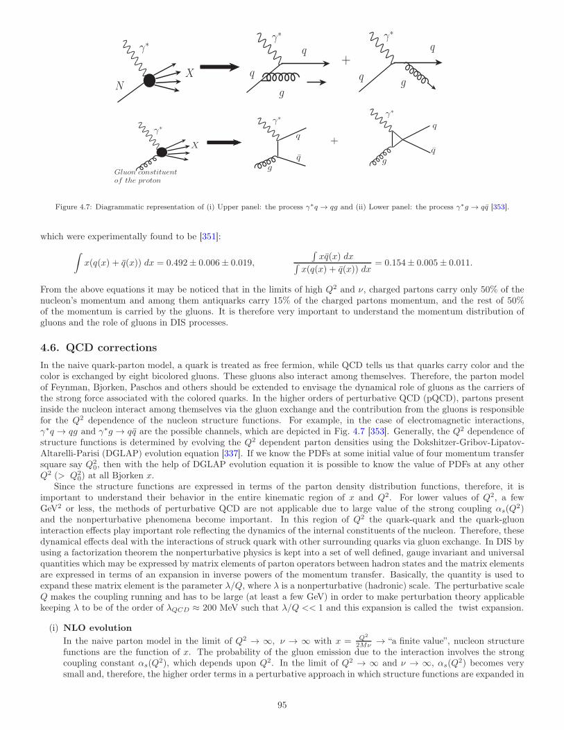
γ∗

NX

γ∗γ∗

gg

+q

q

q

q

γ∗

Gluon constituentof the proton

X

γ∗γ∗

gg

+q

q

q

q

Figure 4.7: Diagrammatic representation of (i) Upper panel: the process γ∗q → qg and (ii) Lower panel: the process γ∗g → qq [353].

which were experimentally found to be [351]:

∫

x(q(x) + q(x)) dx = 0.492± 0.006± 0.019,

∫

xq(x) dx∫

x(q(x) + q(x)) dx= 0.154± 0.005± 0.011.

From the above equations it may be noticed that in the limits of high Q2 and ν, charged partons carry only 50% of thenucleon’s momentum and among them antiquarks carry 15% of the charged partons momentum, and the rest of 50%of the momentum is carried by the gluons. It is therefore very important to understand the momentum distribution ofgluons and the role of gluons in DIS processes.

4.6. QCD corrections

In the naive quark-parton model, a quark is treated as free fermion, while QCD tells us that quarks carry color and thecolor is exchanged by eight bicolored gluons. These gluons also interact among themselves. Therefore, the parton modelof Feynman, Bjorken, Paschos and others should be extended to envisage the dynamical role of gluons as the carriers ofthe strong force associated with the colored quarks. In the higher orders of perturbative QCD (pQCD), partons presentinside the nucleon interact among themselves via the gluon exchange and the contribution from the gluons is responsiblefor the Q2 dependence of the nucleon structure functions. For example, in the case of electromagnetic interactions,γ∗q → qg and γ∗g → qq are the possible channels, which are depicted in Fig. 4.7 [353]. Generally, the Q2 dependence ofstructure functions is determined by evolving the Q2 dependent parton densities using the Dokshitzer-Gribov-Lipatov-Altarelli-Parisi (DGLAP) evolution equation [337]. If we know the PDFs at some initial value of four momentum transfersquare say Q2

0, then with the help of DGLAP evolution equation it is possible to know the value of PDFs at any otherQ2 (> Q2

0) at all Bjorken x.Since the structure functions are expressed in terms of the parton density distribution functions, therefore, it is

important to understand their behavior in the entire kinematic region of x and Q2. For lower values of Q2, a fewGeV2 or less, the methods of perturbative QCD are not applicable due to large value of the strong coupling αs(Q

2)and the nonperturbative phenomena become important. In this region of Q2 the quark-quark and the quark-gluoninteraction effects play important role reflecting the dynamics of the internal constituents of the nucleon. Therefore, thesedynamical effects deal with the interactions of struck quark with other surrounding quarks via gluon exchange. In DIS byusing a factorization theorem the nonperturbative physics is kept into a set of well defined, gauge invariant and universalquantities which may be expressed by matrix elements of parton operators between hadron states and the matrix elementsare expressed in terms of an expansion in inverse powers of the momentum transfer. Basically, the quantity is used toexpand these matrix element is the parameter λ/Q, where λ is a nonperturbative (hadronic) scale. The perturbative scaleQ makes the coupling running and has to be large (at least a few GeV) in order to make perturbation theory applicablekeeping λ to be of the order of λQCD ≈ 200 MeV such that λ/Q << 1 and this expansion is called the twist expansion.

(i) NLO evolution

In the naive parton model in the limit of Q2 → ∞, ν → ∞ with x = Q2

2Mν → “a finite value”, nucleon structurefunctions are the function of x. The probability of the gluon emission due to the interaction involves the strongcoupling constant αs(Q

2), which depends upon Q2. In the limit of Q2 → ∞ and ν → ∞, αs(Q2) becomes very

small and, therefore, the higher order terms in a perturbative approach in which structure functions are expanded in

95

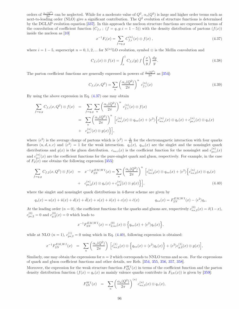
orders of αs(Q2)

2π can be neglected. While for a moderate value of Q2, αs(Q2) is large and higher order terms such as

next-to-leading order (NLO) give a significant contribution. The Q2 evolution of structure functions is determinedby the DGLAP evolution equation [337]. In this approach the nucleon structure functions are expressed in terms ofthe convolution of coefficient function (Cf,i ; (f = q, g; i = 1 − 5)) with the density distribution of partons (f(x))inside the nucleon as [10]

x−1Fi(x) =∑

f=q,g

C(n)f,i (x)⊗ f(x) , (4.37)

where i = 1− 5, superscript n = 0, 1, 2, ... for N(n)LO evolution, symbol ⊗ is the Mellin convolution and

Cf,i(x)⊗ f(x) =∫ 1

x

Cf,i(y) f

(

x

y

)

dy

y. (4.38)

The parton coefficient functions are generally expressed in powers of αs(Q2)

2π as [354]:

Cf,i(x,Q2) =

∑

n

(

αs(Q2)

2π

)n

c(n)f,i (x) (4.39)

By using the above expression in Eq. (4.37) one may obtain

∑

f=q,g

Cf,i(x,Q2)⊗ f(x) =

∑

f=q,g

∑

n

(

αs(Q2)

2π

)n

c(n)f,i (x) ⊗ f(x)

=∑

n

(

αs(Q2)

2π

)n[

c(n)ns,i(x)⊗ qns(x) + 〈e2〉

c(n)ns,i(x)⊗ qs(x) + c

(n)ps,i(x) ⊗ qs(x)

+ c(n)g,i (x)⊗ g(x)

]

,

where 〈e2〉 is the average charge of partons which is 〈e2〉 = 518 for the electromagnetic interaction with four quarks

flavors (u, d, s, c) and 〈e2〉 = 1 for the weak interaction. qs(x), qns(x) are the singlet and the nonsinglet quark

distributions and g(x) is the gluon distribution. cns,i(x) is the coefficient function for the nonsinglet and c(n)ps,i(x)

and c(n)g,i (x) are the coefficient functions for the pure-singlet quark and gluon, respectively. For example, in the case

of F2(x) one obtains the following expression [355]:

∑

f=q,g

Cf,2(x,Q2)⊗ f(x) = x−1FEM,WI

2N (x) =∑

n

(

αs(Q2)

2π

)n[

c(n)ns,2(x) ⊗ qns(x) + 〈e2〉

c(n)ns,2(x) ⊗ qs(x)

+ c(n)ps,2(x)⊗ qs(x) + c

(n)g,2 (x)⊗ g(x)

]

, (4.40)

where the singlet and nonsinglet quark distributions in 4-flavor scheme are given by

qs(x) = u(x) + u(x) + d(x) + d(x) + s(x) + s(x) + c(x) + c(x) qns(x) = FEM,WI2N (x) − 〈e2〉qs,

At the leading order (n = 0), the coefficient functions for the quarks and gluons are, respectively c(0)ns,2(x) = δ(1−x),

c(0)ps,2 = 0 and c

(0)g,2(x) = 0 which leads to

x−1FEM,WI2N (x) = c

(0)2,ns(x) ⊗

qns(x) + 〈e2〉qs(x)

,

while at NLO (n = 1), c(1)ps,2 = 0 using which in Eq. (4.40), following expression is obtained:

x−1FEM,WI2N (x) =

∑

n

(

αs(Q2)

2π

)

[

c(1)ns,2(x)⊗

qns(x) + 〈e2〉qs(x)

+ 〈e2〉c(1)g,2(x)⊗ g(x)]

,

Similarly, one may obtain the expressions for n = 2 which corresponds to NNLO terms and so on. For the expressionsof quark and gluon coefficient functions and other details, see Refs. [354, 355, 356, 357, 358].

Moreover, the expression for the weak structure function FWI3N (x) in terms of the coefficient function and the parton

density distribution function (f(x) = qv(x) as mainly valence quarks contribute in F3N (x)) is given by [359]:

FWI3N (x) =

∑

n

(

αs(Q2)

2π

)(n)

c(n)ns,3(x)⊗ qv(x),

96

where qv(x) is the valence quark distribution and c(n)ns,3(x) is the nonsinglet coefficient function corresponding to the

different perturbative terms including leading order and the other higher order terms. For the detailed discussion,see Refs. [357, 359].

(ii) Target mass corrections (TMC) effectThe target mass correction is a nonperturbative effect which comes into the picture at low Q2, where perturbationtheory fails. The TMC effect is significant at low Q2 and high x, and has been found to be important in thedetermination of the distribution of valence quarks. Unfortunately, this kinematic region has not been exploredmuch, unlike the region of high Q2 and low x. The TMC effect is also known as “kinematic higher twist effect”. In1976, Georgi and Politzer determined the target mass corrections to electroweak structure functions, using operatorproduct expansion (OPE), at the leading order of QCD [360]. Thus these are subleading 1

Q2 corrections to leadingtwist structure functions.

In the QPM, while Q2 → ∞, ν → ∞, mq → 0, with Q2

2Mν = x, the structure functions become the function of x.In the region of low Q2, and in the presence of heavier quarks like charm, bottom, etc., x is modified to ξ which isknown as the Nachtmann variable and is related to the Bjorken variable x as [361]

ξ =2x

1 + ρ; ρ =

√

1 + 4µx2 , µ =M2

Q2, x =

Q2

2Mν. (4.41)

ξ depends only on the hadronic mass and does not have corrections due to the masses of final state quarks. However,for the massive partons, the Nachtmann variable ξ gets modified to the slow rescaling variable ξ. These variables ξand ξ are related as:

ξ = ξ

(

1 +m2

c

Q2

)

=ξ

λ(4.42)

It may be noticed from Eqs. (4.41) and (4.42) that the Nachtmann variable corrects the Bjorken variable for theeffects of hadronic mass while the generalized variable ξ further corrects ξ for the effects of the partonic masses.The simplified expressions of target mass corrected structure functions for massless quarks (u, d, and s) are givenin Ref. [362, 363]. TMC effect has been discussed by several authors such as Scheinbein et al. [361], Ellis et al. [364],Aivazis et al. [365], Brady et al. [366], etc. by taking into account different approaches like the operator productexpansion, collinear factorization, ξ-scaling, and the approach discussed by Ellis-Furmanski-Petronzio [364]. In ournumerical calculations, the nucleon structure functions (FiN (x,Q2); (i = 1− 3)) are evaluated by incorporating theTMC effect following the works of Scheinbein et al. [361].

(iii) Inclusion of charm quark mass effect:Including the mass of charm quark the dimensionless structure functions at NLO are given by [367, 368]

F ci (x,Q

2) = (1− δi4) · s′(ξ, µ2) +αs(µ

2)

2π

∫ 1

ξ

dy′

y′

[

Ciq

(

y′,Q2

µ2, λ)

s′( ξ

y′, µ2)

+ Cig

(

y′,Q2

µ2, λ)

g′( ξ

y′, µ2)]

, (4.43)

for scattering off the CKM rotated weak eigenstate [320]

s′ = s · cos2 θC + d · sin2 θC , (4.44)

and its QCD evolution partner g′

g′ = g · cos2 θC + g · sin2 θC . (4.45)

In Eq. (4.43), Ciq and Ci

g; (i = 1− 5) are respectively the fermionic and gluonic coefficient functions at NLO which

are taken from Ref. [369]. ξ is the slow rescaling variable and the variables λ and y′ are defined as

λ =Q2

(Q2 +m2c), y′ =

ξ

y(4.46)

where mc is the charm quark mass. The terms at the next-to-leading order (Ciq and Ci

g ; (i = 1 − 5)) with strong

coupling constant αs(µ2)

2π gives finite contribution. From the above expression, it may be noticed that though at theleading order F4(x) = 0 but when we have taken NLO terms into account, we obtain a nonzero contribution forF4(x).

(iv) Dynamical higher twist (HT: twist-4) effect:Higher twist is a dynamical effect arising due to the multiparton correlations [370, 371, 372]. This effect involvesthe interactions of struck quark with other quarks via the exchange of gluon and it suppresses by the power of

97

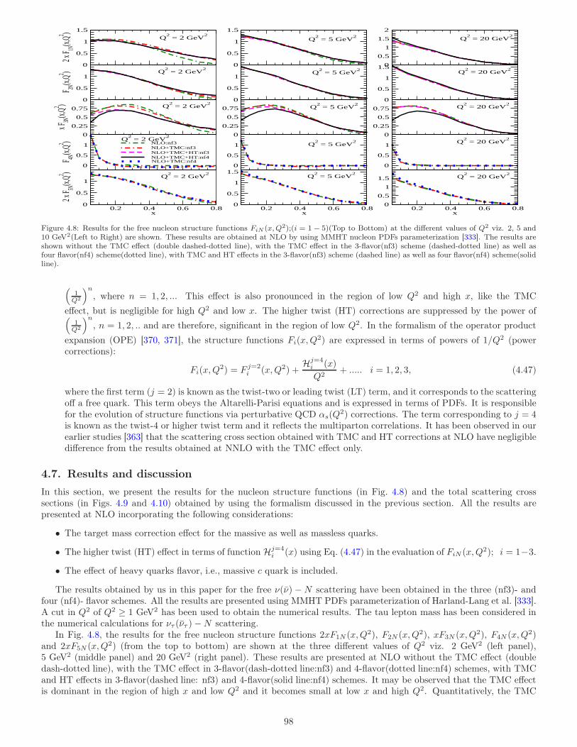
0

0.5

1

1.5

2 x F 1N

(x,Q2 )

NLO:nf3NLO+TMC:nf3NLO+TMC+HT:nf3NLO+TMC+HT:nf4

0

0.5

1

1.5

0

0.5

1

1.5

2

0

0.5

1

F 2N(x,

Q2 )

0

0.5

1

0

0.5

1

1.5

0

0.25

0.5

0.75

x F3N

(x,Q2 )

0

0.25

0.5

0.75

0

0.25

0.5

0.75

0

0.5

1

F 4N(x,

Q2 )

NLO+TMC:nf40

0.5

1

0

0.5

1

0.2 0.4 0.6 0.8x

0

0.5

1

2 x F 5N

(x,Q2 )

0.2 0.4 0.6 0.8x

0

0.5

1

1.5

0.2 0.4 0.6 0.8x

0

0.5

1

1.5

Q2 = 2 GeV

2Q

2 = 5 GeV

2 Q2 = 20 GeV

2

Q2 = 2 GeV

2

Q2 = 2 GeV

2

Q2 = 2 GeV

2

Q2 = 2 GeV

2

Q2 = 5 GeV

2

Q2 = 5 GeV

2

Q2 = 5 GeV

2

Q2 = 5 GeV

2

Q2 = 20 GeV

2

Q2 = 20 GeV

2

Q2 = 20 GeV

2

Q2 = 20 GeV

2

Figure 4.8: Results for the free nucleon structure functions FiN (x,Q2);(i = 1− 5)(Top to Bottom) at the different values of Q2 viz. 2, 5 and10 GeV2(Left to Right) are shown. These results are obtained at NLO by using MMHT nucleon PDFs parameterization [333]. The results areshown without the TMC effect (double dashed-dotted line), with the TMC effect in the 3-flavor(nf3) scheme (dashed-dotted line) as well asfour flavor(nf4) scheme(dotted line), with TMC and HT effects in the 3-flavor(nf3) scheme (dashed line) as well as four flavor(nf4) scheme(solidline).

(

1Q2

)n

, where n = 1, 2, ... This effect is also pronounced in the region of low Q2 and high x, like the TMC

effect, but is negligible for high Q2 and low x. The higher twist (HT) corrections are suppressed by the power of(

1Q2

)n

, n = 1, 2, .. and are therefore, significant in the region of low Q2. In the formalism of the operator product

expansion (OPE) [370, 371], the structure functions Fi(x,Q2) are expressed in terms of powers of 1/Q2 (power

corrections):

Fi(x,Q2) = F j=2

i (x,Q2) +Hj=4

i (x)

Q2+ ..... i = 1, 2, 3, (4.47)

where the first term (j = 2) is known as the twist-two or leading twist (LT) term, and it corresponds to the scatteringoff a free quark. This term obeys the Altarelli-Parisi equations and is expressed in terms of PDFs. It is responsiblefor the evolution of structure functions via perturbative QCD αs(Q

2) corrections. The term corresponding to j = 4is known as the twist-4 or higher twist term and it reflects the multiparton correlations. It has been observed in ourearlier studies [363] that the scattering cross section obtained with TMC and HT corrections at NLO have negligibledifference from the results obtained at NNLO with the TMC effect only.

4.7. Results and discussion

In this section, we present the results for the nucleon structure functions (in Fig. 4.8) and the total scattering crosssections (in Figs. 4.9 and 4.10) obtained by using the formalism discussed in the previous section. All the results arepresented at NLO incorporating the following considerations:

• The target mass correction effect for the massive as well as massless quarks.

• The higher twist (HT) effect in terms of function Hj=4i (x) using Eq. (4.47) in the evaluation of FiN (x,Q2); i = 1−3.

• The effect of heavy quarks flavor, i.e., massive c quark is included.

The results obtained by us in this paper for the free ν(ν) −N scattering have been obtained in the three (nf3)- andfour (nf4)- flavor schemes. All the results are presented using MMHT PDFs parameterization of Harland-Lang et al. [333].A cut in Q2 of Q2 ≥ 1 GeV2 has been used to obtain the numerical results. The tau lepton mass has been considered inthe numerical calculations for ντ (ντ )−N scattering.

In Fig. 4.8, the results for the free nucleon structure functions 2xF1N (x,Q2), F2N (x,Q2), xF3N (x,Q2), F4N (x,Q2)and 2xF5N (x,Q2) (from the top to bottom) are shown at the three different values of Q2 viz. 2 GeV2 (left panel),5 GeV2 (middle panel) and 20 GeV2 (right panel). These results are presented at NLO without the TMC effect (doubledash-dotted line), with the TMC effect in 3-flavor(dash-dotted line:nf3) and 4-flavor(dotted line:nf4) schemes, with TMCand HT effects in 3-flavor(dashed line: nf3) and 4-flavor(solid line:nf4) schemes. It may be observed that the TMC effectis dominant in the region of high x and low Q2 and it becomes small at low x and high Q2. Quantitatively, the TMC

98

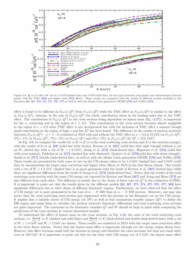
0 10 20 30 40 500

0.1

0.2

0.3

0.4

0.5

σ/E 10

-38 cm

2 GeV

-1

NLO+TMC+HT:W>1.4 GeVNLO+TMC+HT:W>2 GeVKretzer et al.:nocutKretzer et al.: W>1.4 GeVJeong et al.:W>1.4 GeVGazizov et al.Paschos et al.NuWroSHiPHagiwara et al.GENIE

0 10 20 30 40 50E (GeV)

0

0.05

0.1

0.15

0.2

σ /E

10-3

8 cm2 Ge

V-1

DONUT

ντ-N

ν τ-N

nf=4

nf=4

Figure 4.9: σE

vs E with a W cut of 1.4 GeV(dashed line) and 2 GeV(solid line), for tau type neutrinos (top panel) and antineutrinos (bottompanel) with the TMC [369] and higher twist [372] effects. These results are compared with the results of different models available in theliterature [68, 367, 373, 374, 375, 376, 377] as well as with the Monte Carlo generators GENIE [378] and NuWro [379].

effect is found to be different in F2N (x,Q2) from F1N (x,Q2) while the TMC effect in F5N (x,Q2) is similar to the effectin F2N (x,Q2), whereas, in the case of F4N (x,Q2) the whole contribution arises in the leading order due to the TMCeffect. The contribution of F4N (x,Q2) to the cross sections being dependent on lepton mass (Eq. (4.27)), is importantfor the ντ scattering and in the region of x ≤ 0.2. This contribution to the cross section becomes almost negligiblein the region of x > 0.2 when TMC effect is not incorporated but with the inclusion of TMC effect a nonzero thoughsmall contribution in the region of high x and low Q2 has been found. The difference in the results of nucleon structurefunctions FiN (x,Q2); (i = 1−5) evaluated at NLO with and without the TMC effect at x = 0.3 is 5%(3%) in F1N (x,Q2),2%(< 1%) in F2N (x,Q2), 7%(∼ 3%) in F3N (x,Q2) and 4%(∼ 2%) in F5N (x,Q2) for Q2 = 2(5) GeV2.

In Fig. 4.9, we compare the results for σ/E vs E (σ is the total scattering cross section and E is the neutrino energy),with the results of Li et al. [68] (solid line with circles), Kretzer et al. [367] (solid line with right triangle without a cuton W ; dotted line with a cut of W > 1.4 GeV), Jeong et al. [373] (dash-dotted line), Hagiwara et al. [374] (solid linewith cross symbol), Pashchos et al. [375] (dashed line with diamond), Gazizov et al. [376](solid line with down triangle),Anelli et al. [377] (double dash-dotted line), as well as with the Monte Carlo generators GENIE [378] and NuWro [379].These results are presented for both cases of cuts on the CM energy taken to be 1.4 GeV (dashed line) and 2 GeV (solidline) by incorporating the target mass correction and higher twist effects at NLO in the four flavor scheme. Our resultswith a cut of W > 1.4 GeV (dashed line) is in good agreement with the result of Kretzer et al. [367] (dotted line) whilethere are significant differences from the result of Jeong et al. [373] (dash-dotted line). Notice that the results of the totalscattering cross section with the same CM energy cut reported by Kretzer and Reno [367] and Jeong and Reno [373] arealso different from each other. The difference is mainly due to the choice of lower cuts on Q2 in the evaluation of PDFs.It is important to point out that the results given by the different models [68, 367, 373, 374, 375, 376, 377, 380] havesignificant differences due to their choice of different kinematic regions. Furthermore, we have observed that the effectof CM energy cut is more pronounced in the case of ντ − N DIS than in ντ − N DIS process. Moreover, one may alsonotice that the total scattering cross section gets suppressed with the increase in the kinematic cut on the CM energy.It implies that a suitable choice of CM energy cut (W ) as well as four momentum transfer square (Q2) to define theDIS region and using them to calculate the nucleon structure functions, differential and total scattering cross sectionsare quite important. The constrains in the kinematic variables Q2 and W should be kept in mind while comparing thepredictions of the cross sections in various theoretical models.

To understand the effect of lepton mass on the cross sections, in Fig. 4.10, the ratio of the total scattering crosssections, i.e.

σντ−N

σνµ−Nvs E (dashed and solid lines) and

σντ−N

σνµ−Nvs E (dash-dotted and double dash-dotted lines) with a cut

of W > 1.4 GeV and W > 2 GeV are shown. These results are evaluated at NLO with the target mass correction effectin the three flavor scheme. Notice that the lepton mass effect is important through out the energy region shown here.However, this effect becomes small with the increase in energy and therefore the ratio increases but does not reach unityeven at 100 GeV. It is important to point out that for the ratio with CM energy cut of 2 GeV, the lepton mass effect

99

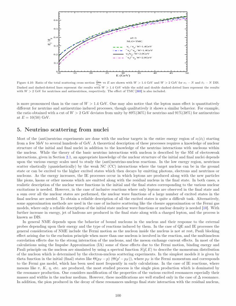
10 15 20 25 30 35 40 45 50E (GeV)

0

0.1

0.2

0.3

0.4

0.5

0.6

σ τ / σµ

ντ / νµ: W>1.4GeV

ν τ/ν µ: W>1.4GeV

ντ/νµ: W>2.0GeV

ν τ/ν µ W>2.0GeV

nf=3

NLO+TMC

Figure 4.10: Ratio of the total scattering cross sectionσντσνµ

vs E are shown with W > 1.4 GeV and W > 2 GeV for ντ −N and ντ −N DIS.

Dashed and dashed-dotted lines represent the results with W > 1.4 GeV while the solid and double dashed-dotted lines represent the resultswith W > 2 GeV for neutrinos and antineutrinos, respectively. The effect of TMC [369] is also included.

is more pronounced than in the case of W > 1.4 GeV. One may also notice that the lepton mass effect is quantitativelydifferent for neutrino and antineutrino induced processes, though qualitatively it shows a similar behavior. For example,the ratio obtained with a cut of W > 2 GeV deviates from unity by 89%(36%) for neutrino and 91%(38%) for antineutrinoat E = 10(50) GeV.

5. Neutrino scattering from nuclei

Most of the (anti)neutrino experiments are done with the nuclear targets in the entire energy region of νl(νl) startingfrom a few MeV to several hundreds of GeV. A theoretical description of these processes requires a knowledge of nuclearstructure of the initial and final nuclei in addition to the knowledge of the neutrino interactions with nucleons withinthe nucleus. While the theory of the basic neutrino interactions with nucleon is described by the SM of electroweakinteractions, given in Section 2.1, an appropriate knowledge of the nuclear structure of the initial and final nuclei dependsupon the various energy scales used to study the (anti)neutrino-nucleus reactions. In the low energy region, neutrinosscatter elastically (quasielastically) by the weak NC (CC) interactions where the target nucleus can be in the groundstate or can be excited to the higher excited states which then decays by emitting photons, electrons and neutrinos ornucleons. As the energy increases, the IE processes occur in which leptons are produced along with the new particleslike pions, kaons or other mesons which are emitted along with the residual nucleus in the final state. In both cases, arealistic description of the nuclear wave functions in the initial and the final states corresponding to the various nuclearexcitations is needed. However, in the case of inclusive reactions where only leptons are observed in the final state anda sum over all the nuclear states are performed, the nuclear wave functions of a large number of excited states in thefinal nucleus are needed. To obtain a reliable description of all the excited states is quite a difficult task. Alternatively,some approximation methods are used in the case of inclusive scattering like the closure approximation or the Fermi gasmodels, where only a reliable description of the initial state nuclear wave functions or nuclear density is needed [10]. Withfurther increase in energy, jet of hadrons are produced in the final state along with a charged lepton, and the process isknown as DIS.

In general NME depends upon the behavior of bound nucleons in the nucleus and their response to the externalprobes depending upon their energy and the type of reactions induced by them. In the case of QE and IE processes thegeneral consideration of NME include the Fermi motion as the nucleon inside the nucleus is not at rest, Pauli blockingeffect arising due to the exclusion principle when more than one nucleon is involved in the reaction, and the multinucleoncorrelation effects due to the strong interaction of the nucleons, and the meson exchange current effects. In most of thecalculations using the Impulse Approximation (IA) some of these effects due to the Fermi motion, binding energy andPauli principle on the nucleon are simulated by using a spectral function S(~p,E) to describe the momentum distributionof the nucleon which is determined by the electron-nucleus scattering experiments. In the simplest models it is given bytheta function in the initial (final) states like Θ(pF − p) (Θ(p′− pF )), where pF is the Fermi momentum and correspondsto the Fermi gas model, which has been used most frequently in early calculations. In the case of IE reactions, wheremesons like π, K, η, etc. are produced, the most studied process is the single pion production which is dominated bythe resonance production. One considers modification of the properties of the various excited resonances especially theirmasses and widths in the nuclear medium. However, these modifications are well studied only in the case of ∆ resonance.In addition, the pion produced in the decay of these resonances undergo final state interaction with the residual nucleus,

100

where elastic scattering, charge exchange process (like π−p → π0n) or pion absorption (π NN → NN) may take place.If the produced pion is absorbed in the nucleus, it mimics a QE-like event. With further increase in energy, the processof DIS takes place in which the (anti)neutrinos interact with the subnucleonic degrees of freedom like the mesons andquarks in the nucleons. In the case of DIS, shadowing and antishadowing corrections become important in the region oflow Bjorken x variable (see Section 5.8). In the intermediate region of x, the mesonic contributions become importantwhere the interaction of an intermediate vector boson (W , Z) takes place with the virtual mesons in the nucleus and inthe region of high x, Fermi motion effects are important.

In the following, we take up the ν(ν)-nucleus scattering in the low, intermediate and high energy region and discussNME.

5.1. Coherent elastic neutrino-nucleus scattering (CEvNS) in the low energy region

The weak NC in the ∆S = 0 sector predicted in the SM allow the existence of the elastic scattering of (anti)neutrinofrom nucleons and nucleus without any threshold constrains and can take place even at very low energies. In the case ofnuclear targets, it was pointed out by Freedman [381] and later by Kopeliovich and Frakfurt [382] that if the (anti)neutrinosenergy and the momentum transfer are too low to induce any excitation or particle emission in the nucleus and the nucleusremains in the ground state, then it is possible that scattering from individual nucleons can be in phase leading to coherentscattering. This coherent scattering would lead to a considerable enhancement in the cross section, which grows withthe increase in the number of nucleons. The necessary condition to observe the phenomenon of coherence in ν-nucleusscattering is that at these (anti)neutrino energies, the momentum transferQ is low enough to satisfy the condition Q≪ 1

R ,where R is the radius of the nucleus.

While the condition of coherence favors the use of the medium and heavy nuclear targets with larger A, it alsopresents formidable problems in its detection. In coherent reactions induced by NC interactions, the only observable isthe recoiling nucleus with a very small kinetic energy i.e. in the energy region of keV for (anti)neutrinos of a few MeVenergy, which is very difficult to measure experimentally. However, the latest developments in the detector technologyhave enabled the measurement of very low energy recoils of nuclei, resulting in the observation of the coherent reactionsfor example by the COHERENT collaboration at ORNL at its spallation neutron source facility using the intense muonneutrino beam obtained from the pions decaying at rest [383]. The first observation of coherent elastic neutrino-nucleusscattering (CEvNS) was reported by this collaboration in CsNaI, using the scintillating crystal detector followed by itsobservation in Ar with a single-phase liquid Ar detector [384] and later with the larger exposure of CsI[Na] [385]. Manynew experiments are planned to be done with other nuclear targets and may be reporting observation of CEvNS in nearfuture [383, 386].

The elastic ν(ν)-nucleus scattering process represented by the reaction

ν(ν) + AZXN −→ ν(ν) + A

ZXN (5.1)

takes place when ν(ν) scatters elastically from the nucleus AZXN which is a composite system of A nucleons. Using

the quantum mechanical principle of superposition, the scattering amplitude F (~k′, ~k) for a ν(ν) with initial and final

momentum ~k and ~k′ respectively, is written as the sum of the scattering amplitude from each nucleon in the nucleus i.e.fj(~k

′, ~k) and is given in the lowest order as:

F (~k′, ~k) =A∑

j=1

fj(~k′, ~k)ei(

~k−~k′).~xj , (5.2)

In the low energy region of the ν(ν), if Q is very small as compared to the inverse of R, i.e. QR << 1, then the scattering

amplitude F (~k′, ~k) becomes the coherent sum of the individual amplitudes from nucleons fj(~k′, ~k) i.e.

F (~k′, ~k) =Z∑

j=1

fpj (~k′, ~k) +

N∑

j=1

fnj (~k′, ~k) (5.3)

and the scattering is called the coherent elastic ν(ν)-nucleus scattering (CEvNS).For the scattering processes induced by the electroweak probes like the electrons and (anti)neutrinos, where the

contribution from the multiple scattering amplitudes are small, Eq. (5.2), gives a satisfactory description of the scatteringin the lowest order. In general, the individual scattering amplitudes are different for the proton and neutron targets innuclei, and the summations over nucleons in Eq. (5.3), runs separately over protons and neutrons. In order to calculate

the scattering amplitudes fj(~k′, ~k) from the individual nucleons in the low energy region, the interaction Lagrangian of

the neutrino and the electron for their interaction with nucleon given by the SM of the electroweak interactions is used.In the SM, the coherent scattering is driven by NC interaction Lagrangian LNC(x) given in Section 1.3, where lNC

µ

and JNCµ are the leptonic and hadronic currents whose matrix elements between the neutrino and the nucleon states

101

is explicitly given in Section 2.1.3. In the region of low energy of the scattering processes, the nucleons are treated asnonrelativistic particles and a nonrelativistic reduction of the matrix elements [10] can be used to calculate the crosssections. The nonrelativistic reduction of the matrix elements [10] shows that in leading order of O( ~q

M ) only the timecomponent of the vector current, with the weak charge operator and the space component of the axial-vector currentwith the spin operator contribute to the matrix elements which give rise to the spin independent and the spin dependentparts of the coherent scattering. Further simplification is achieved if simple scalar and isoscalar nuclear targets with spinzero and N = Z are used as considered in the early works of Freedman [381] and others, where the axial-vector currentsdo not contribute. In general, the contribution of the spin dependent amplitudes to the coherent process is quite smallas compared to the contribution of the spin independent amplitude as the number of unpaired protons (neutrons) in thespin space is quite small as compared to the total number of protons (neutrons) in the nucleus. This has been explicitlyshown recently by Hoferichter et al. [387] and many others quoted in this work. A simple calculation shows that the

differential cross section dσdT , where the recoil energy of the nucleus T ∼ Q2

2MA, with MA being mass of the target nucleus,

is given by [388]:

(

dσ

dT

)

νA

=G2

FMA

2πF 2(Q2)

[

(f1 + g1)2 + (f1 − g1)2

(

1− T

Eν

)2

− (f21 − g21)

MAT

Eν2

]

, (5.4)

and F (Q2) is the nuclear form factor. f1 and g1 are the vector and axial-vector couplings of the neutral vector boson inthe SM to the nucleus A(Z,N) given by:

f1 = fp1Z + fn

1 N ; and g1 = gp1Z + gn1N, (5.5)

where fp(n)1 and g

p(n)1 , respectively, are the vector and axial-vector NC couplings of the (anti)neutrino to the proton (neu-

tron). Neglecting the axial-vector contribution as compared to the contribution of the vector current, we obtain in thecase of isoscalar nuclear targets with spin zero, the expression for the kinetic energy distribution as:

(

dσ

dT

)

νA

≃ G2FMA

2πF 2(Q2)f2

1

[

1 +

(

1− T

Eν

)2

− MAT

Eν2

]

, (5.6)

where f1 is calculated using the SM values of fp1 and fn

1 given by:

fp1 =

1

2− 2 sin2 θW , fn

1 = −1

2(5.7)

leading to(

dσ

dT

)

νA

≃ G2FMA

2πF 2(Q2)

Q2W

4

[

1 +

(

1− T

Eν

)2

− MAT

Eν2

]

, (5.8)

where QW = QnWN +Qp

WZ is called the weak charge of the nucleus with QpW = 1 − 4 sin2 θW and Qn

W = −1 being theweak charges of proton and neutron, respectively. The nuclear form factor F (Q2) is the Fourier transform of the nucleondensity distribution in the nucleus and is given by

F (Q2) = 4π

∫

drr2sin qr

qrρN (r), (5.9)

where ρN (r) is the common density distribution for the protons and neutrons. In case of N 6= Z nuclei and neglectingthe axial contribution, F (Q2)QW is replaced by

F (Q2)QW → Z(1− 4 sin2 θW )Fp(Q2)−NFn(Q

2) (5.10)

with

Fp(Q2) =

4π

Z

∫

drr2sin qr

qrρp(r), Fn(Q

2) =4π

N

∫

drr2sin qr

qrρn(r). (5.11)

The form factor Fp(Q2) obtained from the analysis of electron scattering experiments by Helm [389] and Klein-Nystrand [390]

using the Gaussian or the surface diffuse density distribution are generally used. A similar density distribution for neu-trons Fn(Q

2) with a radius parameter larger than the proton is used. In recent years, theoretical calculations for theseform factors based on the relativistic mean field, energy density functional, shell model and coupled-clusters theory todescribe the nuclear structure have been made [388]. However it has been shown that [387] in the low energy region ofrelevance to the coherent scattering, the nuclear model dependence of the form factors Fp,n(Q

2) is quite small.The numerical values of the weak charges Qp,n

W of protons and neutrons including the radiative corrections are givenby [388, 391]; Qνe,p

W = 0.0766, and Qνe,nW = −1.0233 making the contributions from the protons to the CEvNS very small.

102

Further assuming T << Eν and neglecting the proton contribution, i.e., F 2(Q2)Q2W ≃ F 2

n(Q2)N2, we can write the recoil

energy distribution asdσ

dT≃ G2

FMA

4πN2F 2

n(Q2)

(

1− MAT

2E2ν

)

. (5.12)

In the above expression, radiative corrections have also been not taken into account. Since the CEvNS is an elastic neutralcurrent reaction in which the recoil nucleus is the only observable, therefore, the energy and direction of the recoilingnucleus need to be measured. While the recoil energy distribution is given in Eq. (5.12), the directional distribution isgiven by

dσ

dΩR=

G2F

16π2Q2

W |F (Q2)|2Eν(1 + cos θR). (5.13)

showing that the CEvNS is peaked in the forward direction θR ∼ 0, where θR is the angle between the incoming and theoutgoing neutrinos [388].

The first experimental program to measure the CEvNS cross section was started by the COHERENT collaboration atthe Oak Ridge National Laboratory (ORNL) using its Spallation Neutron Source (SNS) facility using prompt monoener-getic neutrino form π+ → µ+νµ decays and the delayed neutrinos from the subsequent decays of muons i.e. π+ → µ+νµand µ+ → e+νeνµ with continuous energy spectra. These spectra are described by φν(Eν) written as [386]:

φνµ (Eν) =2mπ

m2πm

2µ

δ

(

1− 2Eνmπ

m2π −m2

µ

)

(5.14)

φνe(Eν) =192

mµ

(

Eν

mµ

)2

δ

(

1

2− Eν

mµ

)

(5.15)

φνµ (Eν) =64

mµ

(

Eν

mµ

)2

δ

(

3

4− Eν

mµ

)

. (5.16)

The COHERENT collaboration reported the CEvNS cross sections on CsI(Na) using a crystal detector with a 14.6kg mass target exposed for 308 days with observation of 134±22 events while the SM prediction is 173±48 events [392].A later analysis of the full CsI(Na) data with higher statistics reported the number of events to be 306±20 while theSM prediction is 341 ± 11 (theory) ±42 (expt.) events [393]. The dominant contribution to the systematic uncertaintyis due to the uncertainty in the simulated flux of neutrinos which is around 10%. This corresponds to a flux averagedcross section < σ >= 165+30

−25× 10−40 cm2 and sin2 θW = 0.22± 0.028± 0.026 at Q2 = 50 MeV2 using Helm model for thenuclear form factor.

The second result reported from the COHERENT collaboration is from COH Ar-10 experiment in which a single phaseliquid argon detector was used with 24kg LAr as target and reported the observation of 159±43 CEvNS events [384]. Theuncertainties are due to the uncertainties in the neutrino flux as well as in the neutrino-nucleus cross sections and areabout 13% [384, 394]. This corresponds to the flux averaged cross section of < σ >= 2.2 ± 0.7 × 10−39 cm2 consistentwith the prediction of SM of 1.8 × 10−39 cm2. Both of these cross sections measured in Cs and Ar are within 1σ of theprediction of SM.

Encouraged by these measurements, the COHERENT collaboration has already planned many CEvNS experimentsto be done in future with LAr (24kg), LAr (612kg), Ge (18kg) and NaI(Tl) (3388kg), D2O (600kg), Fe, Pb (1000kg), etc.detectors. The scintillator experiments at other laboratories around the world have been planned proposing other nucleartargets like Xe, Pb, Si, Ge, Cu, etc. However, various experiments proposed for the search of dark matter are developingdetectors which can also be used to observe CEvNS using astrophysical neutrinos from supernovae, solar or atmosphericneutrinos. An excellent compilation of such future experiments is given in Ref. [388].

The physics reach of the CEvNS is very rich. A high precision determination of the CEvNS observables like theenergy and angular distributions of the recoiling nucleus provides opportunity to explore various physics topics becausethe theoretical uncertainties in calculating these observables are quite small. This is because the value of the mixingangle θW in SM and the nuclear form factors in the region of very low momentum transfer are quite well known, the onlyuncertainty arises due to the determination of the neutrino flux, which can be improved in future. In the following, we listsome physics topics in the weak interaction physics where the study of CEvNS is likely to make important contributions:

• Establishes the occurrence of coherence phenomenon in (anti)neutrino-nucleus weak scattering cross sections byconfirming the N2 (Eq. (5.12)) dependence of CEvNS.

• With high precision data and a knowledge of the nuclear form factors directly, determines the weak mixing angleθW and complements its determination from the polarized electron scattering measurements, both of which directlymeasure the weak charge QW in terms of θW .

• CEvNS observables can help to determine the electromagnetic properties of (anti)neutrinos. The electromagneticinteractions being the charge conserving interactions can also contribute to the CEvNS observable with different

103

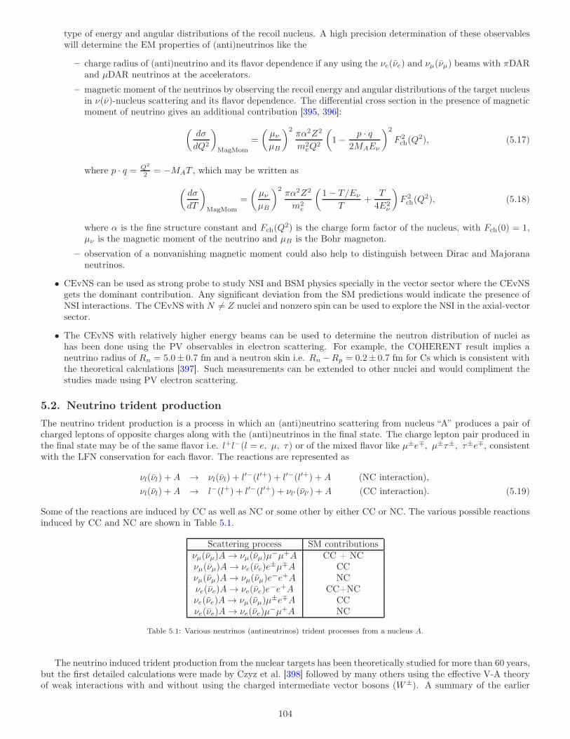
type of energy and angular distributions of the recoil nucleus. A high precision determination of these observableswill determine the EM properties of (anti)neutrinos like the

– charge radius of (anti)neutrino and its flavor dependence if any using the νe(νe) and νµ(νµ) beams with πDARand µDAR neutrinos at the accelerators.

– magnetic moment of the neutrinos by observing the recoil energy and angular distributions of the target nucleusin ν(ν)-nucleus scattering and its flavor dependence. The differential cross section in the presence of magneticmoment of neutrino gives an additional contribution [395, 396]:

(

dσ

dQ2

)

MagMom

=

(

µν

µB

)2πα2Z2

m2eQ

2

(

1− p · q2MAEν

)2

F 2ch(Q

2), (5.17)

where p · q = Q2

2 = −MAT , which may be written as

(

dσ

dT

)

MagMom

=

(

µν

µB

)2πα2Z2

m2e

(

1− T/Eν

T+

T

4E2ν

)

F 2ch(Q

2), (5.18)

where α is the fine structure constant and Fch(Q2) is the charge form factor of the nucleus, with Fch(0) = 1,

µν is the magnetic moment of the neutrino and µB is the Bohr magneton.

– observation of a nonvanishing magnetic moment could also help to distinguish between Dirac and Majorananeutrinos.

• CEvNS can be used as strong probe to study NSI and BSM physics specially in the vector sector where the CEvNSgets the dominant contribution. Any significant deviation from the SM predictions would indicate the presence ofNSI interactions. The CEvNS with N 6= Z nuclei and nonzero spin can be used to explore the NSI in the axial-vectorsector.

• The CEvNS with relatively higher energy beams can be used to determine the neutron distribution of nuclei ashas been done using the PV observables in electron scattering. For example, the COHERENT result implies aneutrino radius of Rn = 5.0± 0.7 fm and a neutron skin i.e. Rn−Rp = 0.2± 0.7 fm for Cs which is consistent withthe theoretical calculations [397]. Such measurements can be extended to other nuclei and would compliment thestudies made using PV electron scattering.

5.2. Neutrino trident production

The neutrino trident production is a process in which an (anti)neutrino scattering from nucleus “A” produces a pair ofcharged leptons of opposite charges along with the (anti)neutrinos in the final state. The charge lepton pair produced inthe final state may be of the same flavor i.e. l+l−(l = e, µ, τ) or of the mixed flavor like µ±e∓, µ±τ±, τ±e∓, consistentwith the LFN conservation for each flavor. The reactions are represented as

νl(νl) +A → νl(νl) + l′−(l′+) + l′−(l′+) +A (NC interaction),

νl(νl) +A → l−(l+) + l′−(l′+) + νl′(νl′) +A (CC interaction). (5.19)

Some of the reactions are induced by CC as well as NC or some other by either CC or NC. The various possible reactionsinduced by CC and NC are shown in Table 5.1.

Scattering process SM contributionsνµ(νµ)A→ νµ(νµ)µ

−µ+A CC + NCνµ(νµ)A→ νe(νe)e

±µ∓A CCνµ(νµ)A→ νµ(νµ)e

−e+A NCνe(νe)A→ νe(νe)e

−e+A CC+NCνe(νe)A→ νµ(νµ)µ

±e∓A CCνe(νe)A→ νe(νe)µ

−µ+A NC

Table 5.1: Various neutrinos (antineutrinos) trident processes from a nucleus A.

The neutrino induced trident production from the nuclear targets has been theoretically studied for more than 60 years,but the first detailed calculations were made by Czyz et al. [398] followed by many others using the effective V-A theoryof weak interactions with and without using the charged intermediate vector bosons (W±). A summary of the earlier

104

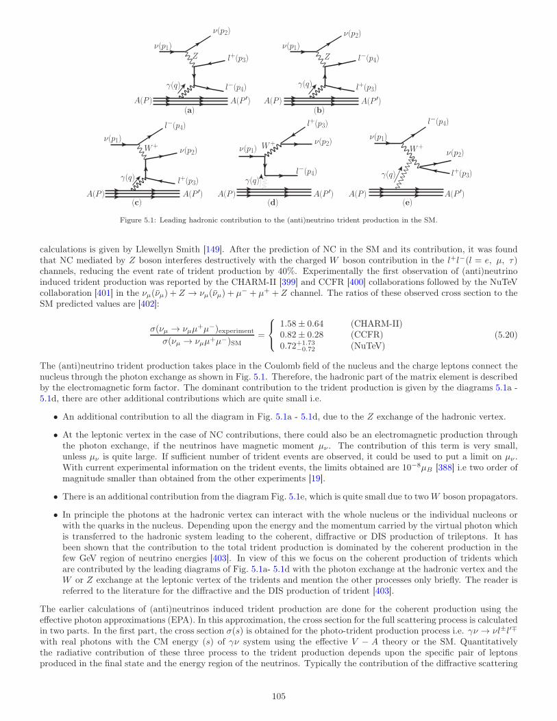
ν(p1)

ν(p2)

Z l+(p3)

l−(p4)γ(q)

A(P ) A(P ′)

ν(p1)

ν(p2)

Z l−(p4)

l+(p3)γ(q)

A(P ) A(P ′)

ν(p1)

l−(p4)

W+ν(p2)

l+(p3)γ(q)

A(P ) A(P ′)

ν(p1)

γ(q)

W+

l+(p3)

l−(p4)

ν(p2)

A(P ) A(P ′)

ν(p1)

l−(p4)

W+ν(p2)

l+(p3)γ(q)

A(P ) A(P ′)

(a) (b)

(c) (d) (e)

Figure 5.1: Leading hadronic contribution to the (anti)neutrino trident production in the SM.

calculations is given by Llewellyn Smith [149]. After the prediction of NC in the SM and its contribution, it was foundthat NC mediated by Z boson interferes destructively with the charged W boson contribution in the l+l−(l = e, µ, τ)channels, reducing the event rate of trident production by 40%. Experimentally the first observation of (anti)neutrinoinduced trident production was reported by the CHARM-II [399] and CCFR [400] collaborations followed by the NuTeVcollaboration [401] in the νµ(νµ) +Z → νµ(νµ) + µ− + µ+ +Z channel. The ratios of these observed cross section to theSM predicted values are [402]:

σ(νµ → νµµ+µ−)experiment

σ(νµ → νµµ+µ−)SM=

1.58± 0.64 (CHARM-II)0.82± 0.28 (CCFR)0.72+1.73

−0.72 (NuTeV)(5.20)

The (anti)neutrino trident production takes place in the Coulomb field of the nucleus and the charge leptons connect thenucleus through the photon exchange as shown in Fig. 5.1. Therefore, the hadronic part of the matrix element is describedby the electromagnetic form factor. The dominant contribution to the trident production is given by the diagrams 5.1a -5.1d, there are other additional contributions which are quite small i.e.

• An additional contribution to all the diagram in Fig. 5.1a - 5.1d, due to the Z exchange of the hadronic vertex.

• At the leptonic vertex in the case of NC contributions, there could also be an electromagnetic production throughthe photon exchange, if the neutrinos have magnetic moment µν . The contribution of this term is very small,unless µν is quite large. If sufficient number of trident events are observed, it could be used to put a limit on µν .With current experimental information on the trident events, the limits obtained are 10−8µB [388] i.e two order ofmagnitude smaller than obtained from the other experiments [19].

• There is an additional contribution from the diagram Fig. 5.1e, which is quite small due to twoW boson propagators.

• In principle the photons at the hadronic vertex can interact with the whole nucleus or the individual nucleons orwith the quarks in the nucleus. Depending upon the energy and the momentum carried by the virtual photon whichis transferred to the hadronic system leading to the coherent, diffractive or DIS production of trileptons. It hasbeen shown that the contribution to the total trident production is dominated by the coherent production in thefew GeV region of neutrino energies [403]. In view of this we focus on the coherent production of tridents whichare contributed by the leading diagrams of Fig. 5.1a- 5.1d with the photon exchange at the hadronic vertex and theW or Z exchange at the leptonic vertex of the tridents and mention the other processes only briefly. The reader isreferred to the literature for the diffractive and the DIS production of trident [403].

The earlier calculations of (anti)neutrinos induced trident production are done for the coherent production using theeffective photon approximations (EPA). In this approximation, the cross section for the full scattering process is calculatedin two parts. In the first part, the cross section σ(s) is obtained for the photo-trident production process i.e. γν → νl±l′∓

with real photons with the CM energy (s) of γν system using the effective V − A theory or the SM. Quantitativelythe radiative contribution of these three process to the trident production depends upon the specific pair of leptonsproduced in the final state and the energy region of the neutrinos. Typically the contribution of the diffractive scattering

105

ν Process ν Process Vijk Aijk Mediator

νe → νee+e− νe → νee

+e− 12 + 2 sin2 θw

12 W,Z

νµ → νµµ+µ− νµ → νµµ

+µ− 12 + 2 sin2 θw

12 W,Z

νe → νµµ+e− νe → νµe

+µ− 1 1 Wνµ → νee

+µ− νµ → νeµ+e− 1 1 W

νe → νeµ+µ− νe → νeµ

+µ− − 12 + 2 sin2 θw − 1

2 Zνµ → νµe

+e− νµ → νµe+e− − 1

2 + 2 sin2 θw − 12 Z

νµ → νµτ+τ− νµ → νµτ

−τ+ − 12 + 2 sin2 θw − 1

2 Zνµ → ντµ

−τ+ νµ → ντµ+τ− 1 1 W

ντ → νµτ−µ+ ντ → νµτ

+µ− 1 1 Wντ → ντµ

+µ− ντ → ντµ−µ+ − 1

2 + 2 sin2 θw − 12 Z

ντ → ντe+e− ντ → ντe

−e+ − 12 + 2 sin2 θw − 1

2 Z

Table 5.2: Modified vector and axial coupling constants for different combinations of incident neutrino flavors and final states

varies between 10% − 40% being largest in the case of µ−µ+ channels but Magill [404] find a larger contribution. Thecontribution of DIS is smaller than 10%.

In the second part, this cross section is multiplied by the probability P (s, q2) of the nucleus producing a virtual photonwith virtuality q2 given by

P (s, q2) =Z2e2

4π2

ds

s

dq2

q2|F (q2)|2, (5.21)

where√s is the CM energy of the incoming neutrino and a real photon system, Ze is the charge and F (q2) is the elec-

tromagnetic from factor of nucleus determined from the electron scattering experiments. In recent years the applicabilityof EPA in the various kinematic regions of s and q2 has been described by some authors and a full calculation in the caseof spin zero nuclei has been done as outlined below [403, 404].

The full matrix elementM for the trident production by the (anti)neutrinos corresponding to the diagrams 5.1a-5.1dis given using the SM as

iM = Lµ(pj, q)−igµνq2

HνX(P, P

′) ; j = 2− 4 (5.22)

The total leptonic amplitude Lµ(pj, q) is given by

Lµ ≡ − ieGF√2

[u(p2)γτ (1− γ5)u(p1)]× u(p4)

[

γτ (Vαβκ −Aαβκγ5)1

(/q − /p3 −m3)γµ

+γµ1

(/p4 − /q −m4)γτ (Vαβκ −Aαβκγ5)

]

v(p3) , (5.23)

and the total hadronic HνX(P, P

′) amplitude is given by

HνX ≡ 〈H(P )|Jν

EM(q2)|H(P ′)〉 , (5.24)

where q ≡ P−P ′ is the four momentum transfer, m3 (m4) the positively (negatively) charged lepton mass, Vαβκ (Aαβκ) ≡gβV (g

βA)δβκ+δαβ (β = α or κ) the vector (axial-vector) couplings, depending on the channel. Jν

EM(q2) is the electromagneticcurrent for the hadronic system A (a nucleus or a nucleon). Vαβk and Aαβk for various processes are given in the Table 5.2.Using this matrix element the differential cross section is given by

d2σνXdQ2ds

=1

32π2(s−M2A)

2

HµνX Lµν

Q4, (5.25)

where

Lµν =1

2s+ 1

∑ ∑

spins

L†µLν , Hµν =

1

2J + 1

∑ ∑

spins

Hµ†Hν . (5.26)

In the case of coherent scattering, the hadronic matrix element is taken as the matrix element of EM current betweennuclear states of initial and final momentum Pµ and P ′µ, and for a spin zero nucleus “A”, it is given by

H = 〈A(P ′)|JµEM |A(P )〉F (Q2)(P + P ′)µ, (5.27)

106

where F (Q2) is the nuclear form factor.In the case of nucleons, the hadronic matrix for protons and neutrons are given as [10]:

〈N(P )|JµEM |N(P ′)〉 = eu(P ′)

[

FN1 (Q2)γµ + iσµνFN

2 (Q2)qν2M

]

u(p) (5.28)

for N = p, n andHµν

N = ZHµνp (P, P ′) + (A− Z)Hµν

n (P, P ′). (5.29)

However, in the case of nucleon N(= n, p), the nucleons are not free but bound with a momentum distribution whichis described by the spectral function S(~p,E). Such spectral functions for nucleon have been determined experimentallyfrom the electron-nucleus scattering from many nuclei and have been used extremely in the calculations of QE ν − Ascattering. The simplest form of S(~p,E) is given by a theta function Θ(PF − P ) in the case of Fermi gas model inwhich the free nucleon cross section is multiplied by a quenching factor R(~q) to obtain the cross section from the boundnucleons [149, 405], i.e.

d2σν−N

dQ2ds→ R(|~q|)d

2σν−N

dQ2ds, (5.30)

where

R(|~q|) =3

2

|~q|2pF

− 1

2

( |~q|2pF

)3

if |~q| < 2pF (5.31)

= 1, if |~q| > 2kF ,

where pF is the Fermi momentum of the nucleons in the nucleus, generally taken to be different for proton and neutronin case of N 6= Z nuclei. Taking the values of the hadronic current given in Eqs. (5.28) and (5.29), the cross sectionis calculated with help of Eq. (5.30). Generally the cross section for the trident production is calculated in terms ofthe photon flux for the longitudinal and transverse photons following the standard procedure. In the region of very lowQ2, Q2 ∼ 0 the contribution from the transverse photons dominates corresponding to the real photons and justifying theuse of EPA in coherent production.

In the case of DIS, the cross section for (anti)neutrino nucleon scattering dσνN

dQ is obtained by convoluting the

(anti)neutrino parton (q) cross sectiondσνq

dQ with nucleon (N = p, n) parton distribution functions fNq (ξ,Q), with Q

being the four momentum transfer and is given by [404]:

σνN =∑

q

∫ 1

ξmin

dξ

∫ Qmax

Qmin

dQdσνq(ξ, q)

dQfNq (ξ,Q), (5.32)

where ξ is the fractional momentum of the partons (q) with ξmin ≥ 0 to enable the creation of lepton pair. With the σνNcalculated from Eq. (5.32), the DIS contribution to the nuclear cross section is obtained using

σνA = Zσνp + (A− Z)σνn. (5.33)

The details for calculatingdσνq

dQ can be found in Ref. [404]. Fig. 5.2 shows some representative results (reactions given in

Table 5.1) for coherent trident cross section of (anti)neutrino scattering on 40Ar and 208Pb [403].In recent years, the rare process of the neutrino trident production has been studied in some detail as a probe of

new physics proposed in many theoretical models of BSM physics which propose the existence of new vector bosons (Z ′)and for new scalar boson (S′), which couple to the leptons and the quarks [404, 406]. The effect of coupling of thesenew bosons to the leptons at the leptonic vertex has been studied for the different values of mass and coupling ofthese bosons and varying them in reasonable limits which are constrained by the limits obtained mainly from the recentexperiment in muon (g − 2) measurements and the limits obtained from the search of such bosons in the BaBar andBelle experiments [407]. In view of the importance of such theoretical studies many experiments to measure the neutrinotrident production with accelerator and atmospheric neutrinos have been proposed.

A summary of the feasibility of seeing neutrino trident production events in these experiments using acceleratorneutrinos has been given by Ballett et al. [403]. On the other hand, the use of atmospheric neutrinos to see the neutrinotrident production in IceCube, ARCA and DeepCore has been discussed by Ge et al. [406].

5.3. Exclusive reactions in ν−nucleus scattering in the low energy region

With the increase in (anti)neutrino energies, corresponding to the de Broglie wavelength of the (anti)neutrinos beingsmaller than the nuclear radius, the interaction takes place with the individual nucleons in the nucleus, leading the targetnucleus to be in any one of its excited states defined by a definite spin (~S), parity (P ) and angular momentum ( ~J)

107

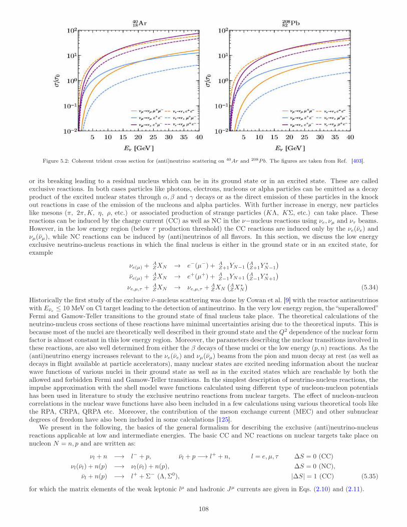
Figure 5.2: Coherent trident cross section for (anti)neutrino scattering on 40Ar and 208Pb. The figures are taken from Ref. [403].

or its breaking leading to a residual nucleus which can be in its ground state or in an excited state. These are calledexclusive reactions. In both cases particles like photons, electrons, nucleons or alpha particles can be emitted as a decayproduct of the excited nuclear states through α, β and γ decays or as the direct emission of these particles in the knockout reactions in case of the emission of the nucleons and alpha particles. With further increase in energy, new particleslike mesons (π, 2π,K, η, ρ, etc.) or associated production of strange particles (KΛ, KΣ, etc.) can take place. Thesereactions can be induced by the charge current (CC) as well as NC in the ν−nucleus reactions using νe, νµ and ντ beams.However, in the low energy region (below τ production threshold) the CC reactions are induced only by the νe(νe) andνµ(νµ), while NC reactions can be induced by (anti)neutrinos of all flavors. In this section, we discuss the low energyexclusive neutrino-nucleus reactions in which the final nucleus is either in the ground state or in an excited state, forexample

νe(µ) +AZXN → e−(µ−) + A

Z+1YN−1

(

AZ+1Y

∗N−1

)

νe(µ) +AZXN → e+(µ+) + A

Z−1YN+1

(

AZ−1Y

∗N+1

)

νe,µ,τ + AZXN → νe,µ,τ + A

ZXN

(

AZX

∗N

)

(5.34)

Historically the first study of the exclusive ν-nucleus scattering was done by Cowan et al. [9] with the reactor antineutrinoswith Eνe ≤ 10 MeV on Cl target leading to the detection of antineutrino. In the very low energy region, the “superallowed”Fermi and Gamow-Teller transitions to the ground state of final nucleus take place. The theoretical calculations of theneutrino-nucleus cross sections of these reactions have minimal uncertainties arising due to the theoretical inputs. This isbecause most of the nuclei are theoretically well described in their ground state and the Q2 dependence of the nuclear formfactor is almost constant in this low energy region. Moreover, the parameters describing the nuclear transitions involved inthese reactions, are also well determined from either the β decays of these nuclei or the low energy (p, n) reactions. As the(anti)neutrino energy increases relevant to the νe(νe) and νµ(νµ) beams from the pion and muon decay at rest (as well asdecays in flight available at particle accelerators), many nuclear states are excited needing information about the nuclearwave functions of various nuclei in their ground state as well as in the excited states which are reachable by both theallowed and forbidden Fermi and Gamow-Teller transitions. In the simplest description of neutrino-nucleus reactions, theimpulse approximation with the shell model wave functions calculated using different type of nucleon-nucleon potentialshas been used in literature to study the exclusive neutrino reactions from nuclear targets. The effect of nucleon-nucleoncorrelations in the nuclear wave functions have also been included in a few calculations using various theoretical tools likethe RPA, CRPA, QRPA etc. Moreover, the contribution of the meson exchange current (MEC) and other subnucleardegrees of freedom have also been included in some calculations [125].

We present in the following, the basics of the general formalism for describing the exclusive (anti)neutrino-nucleusreactions applicable at low and intermediate energies. The basic CC and NC reactions on nuclear targets take place onnucleon N = n, p and are written as:

νl + n −→ l− + p, νl + p −→ l+ + n, l = e, µ, τ ∆S = 0 (CC)

νl(νl) + n(p) −→ νl(νl) + n(p), ∆S = 0 (NC),

νl + n(p) −→ l+ +Σ− (Λ,Σ0), |∆S| = 1 (CC) (5.35)

for which the matrix elements of the weak leptonic lµ and hadronic Jµ currents are given in Eqs. (2.10) and (2.11).

108

In case of the nucleons bound in the nucleus, these matrix elements are to be taken between the initial (|i〉) andfinal (|f〉) nuclear states i.e.

MCC(NC)fi = 〈f |HCC(NC)

W |i〉,

where H = −GF a√2

∫

d~x lµCC(NC) JCC(NC)µ (x), (5.36)

lµCC(NC) is the leptonic current, JCC(NC)µ is the hadronic current operator in the nucleus and a = cos θC(1) for CC (NC)

induced processes, and are given in Eq. (2.10) and (2.18) in the SM.Since the leptons in Eq. (5.35) are free point particles, therefore, we can describe them by plane waves (neglecting the

Coulomb effect of the charged lepton in final state) to write

lµ(x) = lµe−i~q·~x, q = k′ − k = p− p′. (5.37)

such that the matrix element Mfi between the initial (|i〉) and final (|f〉) states, using the notation lµ for lµCC(NC) and

Jµ for JCC(NC)µ for simplicity, is written as

Mfi = −GF a√2〈f |∫

e−i~q·~xlµJµ(x)d~x|i〉 = −GF a√

2〈f |∫

e−i~q·~x(l0J0 −~l · ~J)d~x|i〉. (5.38)

The matrix element Mfi is calculated using the multipole expansion of the e−i~q·~x and ~le−i~q·~x. For that we write

~l =∑

λ=0,±1

lλe†λ, (5.39)

where eλ(λ = ±1, 0) are the components of the unit vector (ex, ey, ez) in the spherical basis defined as

e±1 = ± ex ± iey√2

, e0 = ez, ~eλ · ~eλ′ = δλλ′ , such that lλ =∑

~l · eλ (5.40)

and write

ei~q·~x =

∞∑

l=0

√

4π(2l + 1) iljl(qx)Yl0(Ωx), (5.41)

where Yl0(Ωx) are the spherical harmonics and jJ (qx) are the spherical Bessel’s function.

Using the definition of the vector spherical harmonics ~YMJl1 defined as

~YMJl1 =

∑

mλ

〈lm1λ|l1JM〉Ylm(θ, φ)~eλ, (5.42)

where 〈lm1|λ|l1JM〉 is the Clebsch-Gordan (CG) coefficients and choosing q ‖ eZ i.e. unit vector along z axis, we canwrite

~eλei~q·~x =

∑

l

∞∑

J=0

√

4π(2l+ 1) iJjl(qx)〈l01λ|l1Jλ〉~YλJL1, x = |~x|, q = |~q|. (5.43)

In Eq. (5.43), we perform the expansion over l, using the values of the CG coefficients for λ = ±1 and = 0 explicitly.There would be, in general, three terms for each λ(= ±1, 0), corresponding to l = J +1, J, J − 1. Using the nonvanishing

values of CG coefficients in each case and the following properties of the vector spherical harmonics ~YMJl1 i.e. [408]:

~∇r × jJ (r)~YMJJ1 = −i

( J

2J + 1

)12

jJ+1(r)~YMJ,J+1,1 + i

( J + 1

2J + 1

)12

jJ−1(r)~YMJ,J−1,1, (5.44)

~∇rjJ(r)YJM =( J + 1

2J + 1

)12

jJ+1(r)~YMJ,J+1,1

( J

2J + 1

)12

jJ−1(r)~YMJ,J−1,1, (5.45)

the expression for ~eλei~q·~x given in Eq. (5.43) is evaluated.

After performing some basic algebraic manipulations, the following expressions are obtained [10]:

~e~qλei~q·~x = − i

q

∞∑

J=0

[4π(2J + 1)]12 iJ ~∇(jJ (qx)YJ0(Ωx)), for λ = 0

= −∞∑

J≥1

[2π(2J + 1)]12 iJ[

λjJ (qx)~YλJJ1 +

1

q~∇× (jJ (qx))~Yλ

JJ1

]

, for λ = ±1. (5.46)

109

Therefore, the matrix element in Eq. (5.38) is written using Eq. (5.46) as [10]

〈f |HW |i〉 = +G√2〈f |(

∞∑

J=0

[4π(2J + 1)]12 (−i)J [l3LJ0(q) − l0CJ0(q)]

−∑

λ=±1

lλ

∞∑

J≥1

[2π(2J + 1)]12 (−i)J × [λTmag

J−λ (q) + T elJ−λ(q)]

)

|i〉, (5.47)

where

CJM (q) ≡∫

d~x[jJ (qx)YJM (Ωx)]J0(~x); LJM (q) ≡ i

q

∫

d~x[~∇(jJ (qx)YJM (Ωx))] · ~J(~x), (5.48)

T elJM (q) ≡ i

q

∫

d~x[~∇×~jJ(qx)~YMJJ1 ] · ~J(~x); Tmag

JM (q) ≡∫

d~x[jJ (qx)~YMJJ1] · ~J(~x), (5.49)

and are called multipoles.In the following, we enumerate some features of the above multipoles:

(i) The CJM (q), LJM (q), T elJM (q) and Tmag

JM (q) are called, respectively, the Coulomb, longitudinal, transverse electric,and transverse magnetic multipoles.

(ii) The weak current operator Jµ(J0, ~J) appearing in the definition of multipoles contains vector (V µ) and axial-vector(Aµ) currents in both cases of CC and NC reactions. Therefore, each multipole (MJM = CJM , LJM , T

elJM , T

magJM )

consists of the vector and axial-vector multipoles and is generally written as:

MJM −→MVJM (q) +MA

JM (q),

where MVJM (q) and MA

JM (q) are the multipoles corresponding to vector and axial-vector currents.

(iii) The parity of MVJM is defined in the conventional way with reference to the electromagnetic vector current. The

parity of the vector (MVJM (q)) and axial-vector (MA

JM (q)) multipoles and are opposite to each other, which areshown in Table-5.3.

Multipole CVJM LV

JM T el,VJM Tmag,V

JM CAJM LA

JM T el,AJM Tmag,A

JM

Parity (−1)J (−1)J (−1)J (−1)J+1 (−1)J+1 (−1)J+1 (−1)J+1 (−1)J

Table 5.3: Parity of vector and axial-vector multipoles.

(iv) In general, there are 8 multipoles to be considered, four corresponding to the vector currents and four correspondingto the axial-vector currents. However, since the vector current is conserved i.e.

qµJµ = 0 ⇒ q0J

0 = ~q · ~J. (5.50)

Taking ~q ‖ ez, we get a relation between the Coulomb and longitudinal multipoles i.e.

q0〈Jf |CVJM |Ji〉 − qZ〈Jf |LV

JM |Ji〉 = 0. (5.51)

Therefore, the ν(ν) cross sections are given in terms of seven multipoles while the electron scattering is describedin terms of three multipoles.

(v) The single nucleon current operators (J0, ~J) to be used with the nuclear wave functions in the impulse approxi-mation are derived from the definition of the vector and axial-vector current operators for the free nucleon givenin Section 2.1. In the case of a nucleus, the nucleons are treated nonrelativistically, therefore, the nonrelativisticreduction of the current operators can be used. In the case of CC reactions, we obtain Jµ

CC in the lowest order of

momenta, neglecting the term O(

~q 2

M2

)

, O(

~p 2

M2

)

as [10]

J0CC =

(

f1(q2) + g1(q

2)~σ · 2~p− ~q2M

)

τ± (5.52)

~JCC =

(

g1(q2)~σ − i(f1(q2) + f2(q

2))~σ × ~q2M

)

τ± + f1(q2)2~p− ~q2M

τ±. (5.53)

110

The operator τ+(−) corresponds to the ν(ν) scattering processes. Similar expressions are obtained for the NCinteractions with f1(q

2), f2(q2) and g1(q

2) replaced by NC form factors f1(q2), f2(q

2) and g1(q2) and τ+(−) replaced

by the isoscalar (1 ) and isovector operators (τ3) depending upon the isospin structure of JµNC .

It should be noted that the terms involving q02M are of the order of O

(

q 2

4M2

)

as q0 = − q2

2M for elastic scattering andare, therefore, neglected in the case of nuclear transitions at low energies. The nuclear operators corresponding tothe nucleon operators given in Eqs. (5.52) and (5.53) are, therefore, written in the impulse approximation as

J0s(x) =

A∑

j=1

[

f1(q2) + g1(q

2)

(

p(j)

Mδ(x− x0)

)

sym

]

τ±δ(~x − ~xj) (5.54)

~Js(x) =

A∑

j=1

[

g1(q2)~σ + f1(q

2)2~p · ~q2M

− i f1(q2) + 2M(q2)

2M~σ(j)× ~q

]

τ±δ(~x− ~xj), (5.55)

where ~xj is the position coordinate of the interacting nucleon. This shows that various operators in the nuclear space

which enter in the current J0(x) and ~J(x) operators are the type τ±(j), τ±(j)σ(j) and τ±(j)~p(j)(= −iτ±(j)~∇(j))multiplied by the spherical harmonics YJM , vector spherical harmonics (~YJMl) and the gradient ~∇ · ~Y and the curl

operators (~∇× ~Y ) of the vector spherical harmonics as shown in the definition of the multipoles in Eqs. (5.48) and(5.49).

Using the matrix element in Eq. (5.38), the cross section is calculated for the transition between the initial state |i〉 andthe final state |f〉 of the nucleus which are defined by the definite angular momenta and parity as |JiMi〉 and |JfMf〉 andis given by

dσ

dΩ=k′E′

4π2

∑

lepton spins

1

2Ji + 1

∑

Mi

∑

Mf

| 〈JfMf | H |JiMi〉 |2 (5.56)

Since the matrix element of H is written in terms of the various multipoles with definite angular momentum and parity,|Jλ〉 (see Eqs. (5.48)–(5.49)) the standard angular momentum algebra can be used to calculate the cross section given inEq. (5.56). In the limit of ultrarelativistic lepton in the final states [10]:

(

dσ

dΩ

)RL

νν

=G2ǫ2

4π2

4π

2Ji + 1

[

cos2 θC

( ∞∑

J=0

|⟨

Jf

∣

∣

∣

∣

∣

∣

∣

∣

MJ −q0

~qLJ

∣

∣

∣

∣

∣

∣

∣

∣

Ji

⟩

|2)

+

(

q2

2|~q |2 cos2θ

2+ sin2

θ

2

)

∞∑

J≥1

(

|〈Jf ||TmagJ ||Ji〉|2 + |〈Jf ||T el

J ||Ji〉|2)

∓ sinθ

2

1

|~q |

(

q2 cos2θ

2+ |~q |2 sin2 θ

2

)1/2(

2 Re〈Jf ||TmagJ ||Ji〉〈Jf ||T el

J ||Ji〉∗)

]

, (5.57)

where 〈Jf | | ~J | |Ji〉 is the reduced matrix element of the multipole MMJ with angular momentum ~J . In the case of very low

energy (anti)neutrinos from solar or reactor sources, the expression contains terms dependent upon the lepton velocityβ(= v

c ).In order to calculate the nuclear matrix elements, we need the nuclear wave functions for |i〉 and |f〉 states which are

essentially the nonrelativistic wave functions of nucleons bound in a nucleus by a nucleon-nucleon potential.The nuclear states |i〉 and |f〉 characterized by the angular momentum (and parity) |JiMi〉 and |JfMf〉 are generally

expressed as:

|i〉 ≡ |JiMi〉 ≡ ψnl 12JiMi(~x) = NRnl(r)[Ylml

(θ, φ)⊗ Y 12ms

]JiMi(5.58)

and |f〉 = |JfMf〉 = ψn′l′ 12JfMf

(~x) = N ′Rn′l′(r)[Yl′m′(θ, φ)⊗ Y 12ms′

]JfMf(5.59)

where Rnl(r) and Rn′l′(r) are the radial wave functions of the initial and final nucleus obtained by solving the Schrödingerequations for nucleons moving in a central potential like the harmonic oscillator potential. In a more sophisticateddescription of the nuclear wave functions various forms of the nucleon-nucleon potentials are included to describe theresidual interactions to take into account the effect of pairing and other nucleon-nucleon correlation effects [10]. Usingthese wave functions and the transition current operators written in Eqs. (5.54) and (5.55), and the multipoles defined inEqs. (5.48)–(5.49), the matrix element defined in Eq. (5.38) are calculated. The expressions for the matrix elements forvarious multipoles using the harmonic oscillator wave functions have been given by Haxton [409].

Eq. (5.57) is the general result which is used to calculate the nuclear cross section for QE ν and ν reactions leadingto discrete nuclear states in various nuclei from deuterons to medium and heavy nuclei. Once the initial and final states

111

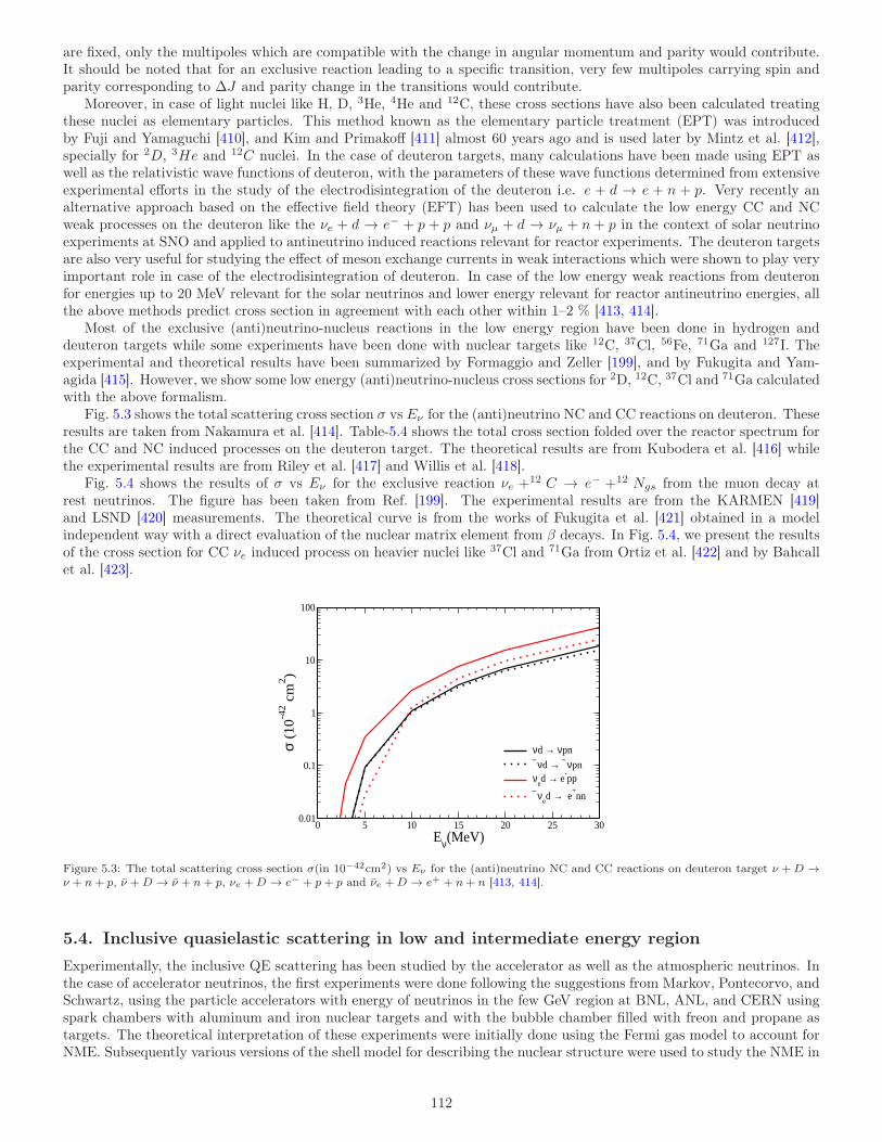
are fixed, only the multipoles which are compatible with the change in angular momentum and parity would contribute.It should be noted that for an exclusive reaction leading to a specific transition, very few multipoles carrying spin andparity corresponding to ∆J and parity change in the transitions would contribute.

Moreover, in case of light nuclei like H, D, 3He, 4He and 12C, these cross sections have also been calculated treatingthese nuclei as elementary particles. This method known as the elementary particle treatment (EPT) was introducedby Fuji and Yamaguchi [410], and Kim and Primakoff [411] almost 60 years ago and is used later by Mintz et al. [412],specially for 2D, 3He and 12C nuclei. In the case of deuteron targets, many calculations have been made using EPT aswell as the relativistic wave functions of deuteron, with the parameters of these wave functions determined from extensiveexperimental efforts in the study of the electrodisintegration of the deuteron i.e. e + d → e + n + p. Very recently analternative approach based on the effective field theory (EFT) has been used to calculate the low energy CC and NCweak processes on the deuteron like the νe + d → e− + p + p and νµ + d → νµ + n + p in the context of solar neutrinoexperiments at SNO and applied to antineutrino induced reactions relevant for reactor experiments. The deuteron targetsare also very useful for studying the effect of meson exchange currents in weak interactions which were shown to play veryimportant role in case of the electrodisintegration of deuteron. In case of the low energy weak reactions from deuteronfor energies up to 20 MeV relevant for the solar neutrinos and lower energy relevant for reactor antineutrino energies, allthe above methods predict cross section in agreement with each other within 1–2 % [413, 414].

Most of the exclusive (anti)neutrino-nucleus reactions in the low energy region have been done in hydrogen anddeuteron targets while some experiments have been done with nuclear targets like 12C, 37Cl, 56Fe, 71Ga and 127I. Theexperimental and theoretical results have been summarized by Formaggio and Zeller [199], and by Fukugita and Yam-agida [415]. However, we show some low energy (anti)neutrino-nucleus cross sections for 2D, 12C, 37Cl and 71Ga calculatedwith the above formalism.

Fig. 5.3 shows the total scattering cross section σ vs Eν for the (anti)neutrino NC and CC reactions on deuteron. Theseresults are taken from Nakamura et al. [414]. Table-5.4 shows the total cross section folded over the reactor spectrum forthe CC and NC induced processes on the deuteron target. The theoretical results are from Kubodera et al. [416] whilethe experimental results are from Riley et al. [417] and Willis et al. [418].

Fig. 5.4 shows the results of σ vs Eν for the exclusive reaction νe +12 C → e− +12 Ngs from the muon decay atrest neutrinos. The figure has been taken from Ref. [199]. The experimental results are from the KARMEN [419]and LSND [420] measurements. The theoretical curve is from the works of Fukugita et al. [421] obtained in a modelindependent way with a direct evaluation of the nuclear matrix element from β decays. In Fig. 5.4, we present the resultsof the cross section for CC νe induced process on heavier nuclei like 37Cl and 71Ga from Ortiz et al. [422] and by Bahcallet al. [423].

0 5 10 15 20 25 30Eν(MeV)

0.01

0.1

1

10

100

σ (1

0-42 c

m2 )

νd → νpn

ν d → ν pnν

ed → e-

pp

νed → e+

nn

Figure 5.3: The total scattering cross section σ(in 10−42cm2) vs Eν for the (anti)neutrino NC and CC reactions on deuteron target ν +D →ν + n+ p, ν +D → ν + n+ p, νe +D → e− + p+ p and νe +D → e+ + n+ n [413, 414].

5.4. Inclusive quasielastic scattering in low and intermediate energy region

Experimentally, the inclusive QE scattering has been studied by the accelerator as well as the atmospheric neutrinos. Inthe case of accelerator neutrinos, the first experiments were done following the suggestions from Markov, Pontecorvo, andSchwartz, using the particle accelerators with energy of neutrinos in the few GeV region at BNL, ANL, and CERN usingspark chambers with aluminum and iron nuclear targets and with the bubble chamber filled with freon and propane astargets. The theoretical interpretation of these experiments were initially done using the Fermi gas model to account forNME. Subsequently various versions of the shell model for describing the nuclear structure were used to study the NME in

112

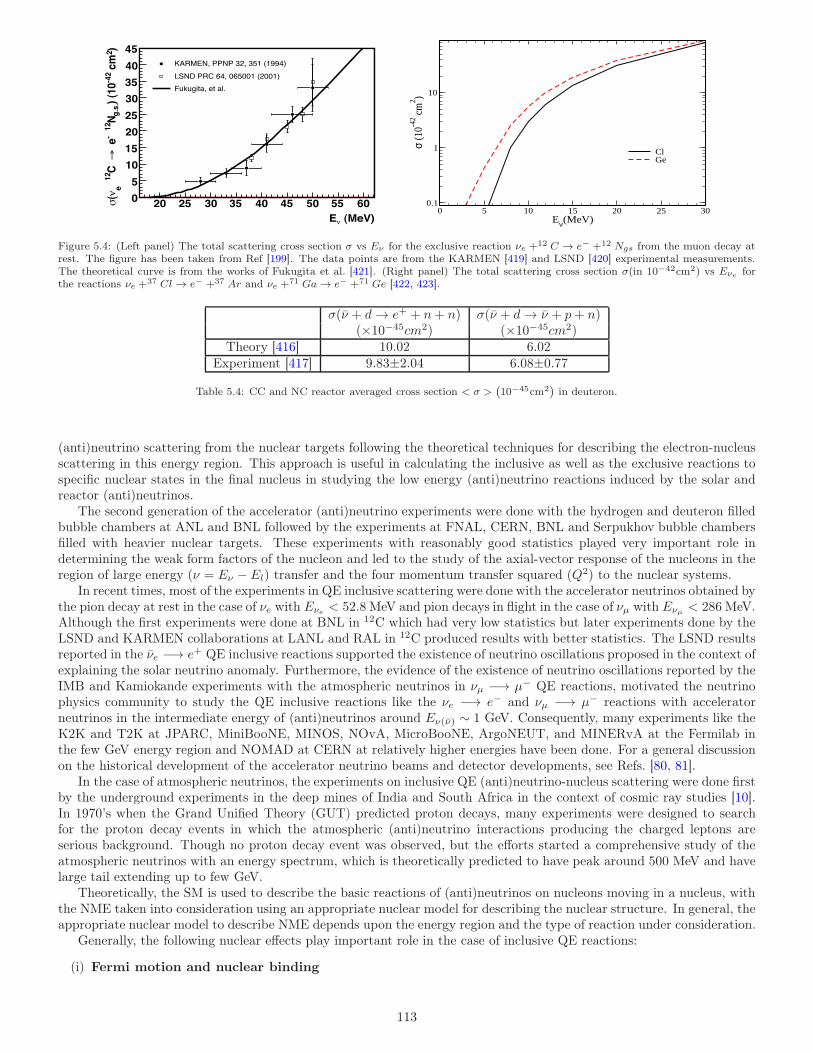
(MeV) E

20 25 30 35 40 45 50 55 60

)2 c

m-4

2)

(10

g.s

.N

12

-

e!

C

12

e

(" 0

5

10

15

20

25

30

35

40

45

KARMEN, PPNP 32, 351 (1994)

LSND PRC 64, 065001 (2001)

Fukugita, et al.

0 5 10 15 20 25 30Eν(MeV)

0.1

1

10

σ (1

0-42 c

m2 )

ClGe

Figure 5.4: (Left panel) The total scattering cross section σ vs Eν for the exclusive reaction νe +12 C → e− +12 Ngs from the muon decay atrest. The figure has been taken from Ref [199]. The data points are from the KARMEN [419] and LSND [420] experimental measurements.The theoretical curve is from the works of Fukugita et al. [421]. (Right panel) The total scattering cross section σ(in 10−42cm2) vs Eνe forthe reactions νe +37 Cl → e− +37 Ar and νe +71 Ga → e− +71 Ge [422, 423].

σ(ν + d→ e+ + n+ n) σ(ν + d→ ν + p+ n)(×10−45cm2) (×10−45cm2)

Theory [416] 10.02 6.02Experiment [417] 9.83±2.04 6.08±0.77

Table 5.4: CC and NC reactor averaged cross section < σ >(

10−45cm2)

in deuteron.

(anti)neutrino scattering from the nuclear targets following the theoretical techniques for describing the electron-nucleusscattering in this energy region. This approach is useful in calculating the inclusive as well as the exclusive reactions tospecific nuclear states in the final nucleus in studying the low energy (anti)neutrino reactions induced by the solar andreactor (anti)neutrinos.

The second generation of the accelerator (anti)neutrino experiments were done with the hydrogen and deuteron filledbubble chambers at ANL and BNL followed by the experiments at FNAL, CERN, BNL and Serpukhov bubble chambersfilled with heavier nuclear targets. These experiments with reasonably good statistics played very important role indetermining the weak form factors of the nucleon and led to the study of the axial-vector response of the nucleons in theregion of large energy (ν = Eν − El) transfer and the four momentum transfer squared (Q2) to the nuclear systems.

In recent times, most of the experiments in QE inclusive scattering were done with the accelerator neutrinos obtained bythe pion decay at rest in the case of νe with Eνe < 52.8 MeV and pion decays in flight in the case of νµ with Eνµ < 286 MeV.Although the first experiments were done at BNL in 12C which had very low statistics but later experiments done by theLSND and KARMEN collaborations at LANL and RAL in 12C produced results with better statistics. The LSND resultsreported in the νe −→ e+ QE inclusive reactions supported the existence of neutrino oscillations proposed in the context ofexplaining the solar neutrino anomaly. Furthermore, the evidence of the existence of neutrino oscillations reported by theIMB and Kamiokande experiments with the atmospheric neutrinos in νµ −→ µ− QE reactions, motivated the neutrinophysics community to study the QE inclusive reactions like the νe −→ e− and νµ −→ µ− reactions with acceleratorneutrinos in the intermediate energy of (anti)neutrinos around Eν(ν) ∼ 1 GeV. Consequently, many experiments like theK2K and T2K at JPARC, MiniBooNE, MINOS, NOvA, MicroBooNE, ArgoNEUT, and MINERvA at the Fermilab inthe few GeV energy region and NOMAD at CERN at relatively higher energies have been done. For a general discussionon the historical development of the accelerator neutrino beams and detector developments, see Refs. [80, 81].

In the case of atmospheric neutrinos, the experiments on inclusive QE (anti)neutrino-nucleus scattering were done firstby the underground experiments in the deep mines of India and South Africa in the context of cosmic ray studies [10].In 1970’s when the Grand Unified Theory (GUT) predicted proton decays, many experiments were designed to searchfor the proton decay events in which the atmospheric (anti)neutrino interactions producing the charged leptons areserious background. Though no proton decay event was observed, but the efforts started a comprehensive study of theatmospheric neutrinos with an energy spectrum, which is theoretically predicted to have peak around 500 MeV and havelarge tail extending up to few GeV.

Theoretically, the SM is used to describe the basic reactions of (anti)neutrinos on nucleons moving in a nucleus, withthe NME taken into consideration using an appropriate nuclear model for describing the nuclear structure. In general, theappropriate nuclear model to describe NME depends upon the energy region and the type of reaction under consideration.

Generally, the following nuclear effects play important role in the case of inclusive QE reactions:

(i) Fermi motion and nuclear binding

113

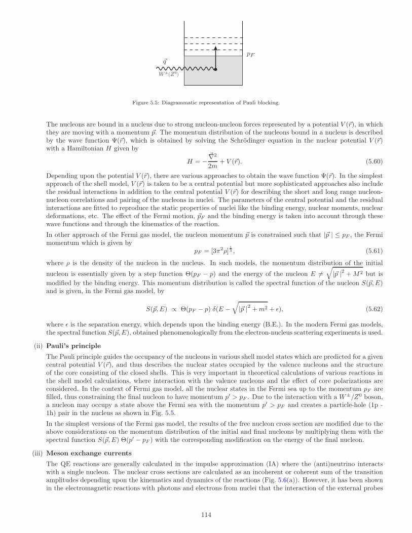
W±(Z0)

~qpF

Figure 5.5: Diagrammatic representation of Pauli blocking.

The nucleons are bound in a nucleus due to strong nucleon-nucleon forces represented by a potential V (~r), in whichthey are moving with a momentum ~p. The momentum distribution of the nucleons bound in a nucleus is describedby the wave function Ψ(~r), which is obtained by solving the Schrödinger equation in the nuclear potential V (~r)with a Hamiltonian H given by

H = −~∇2

2m+ V (~r). (5.60)

Depending upon the potential V (~r), there are various approaches to obtain the wave function Ψ(~r). In the simplestapproach of the shell model, V (~r) is taken to be a central potential but more sophisticated approaches also includethe residual interactions in addition to the central potential V (~r) for describing the short and long range nucleon-nucleon correlations and pairing of the nucleons in nuclei. The parameters of the central potential and the residualinteractions are fitted to reproduce the static properties of nuclei like the binding energy, nuclear moments, nucleardeformations, etc. The effect of the Fermi motion, ~pF and the binding energy is taken into account through thesewave functions and through the kinematics of the reaction.

In other approach of the Fermi gas model, the nucleon momentum ~p is constrained such that |~p | ≤ pF , the Fermimomentum which is given by

pF = [3π2ρ]13 , (5.61)

where ρ is the density of the nucleon in the nucleus. In such models, the momentum distribution of the initial

nucleon is essentially given by a step function Θ(pF − p) and the energy of the nucleon E 6=√

|~p |2 +M2 but is

modified by the binding energy. This momentum distribution is called the spectral function of the nucleon S(~p,E)and is given, in the Fermi gas model, by

S(~p,E) ∝ Θ(pF − p) δ(E −√

|~p |2 +m2 + ǫ), (5.62)

where ǫ is the separation energy, which depends upon the binding energy (B.E.). In the modern Fermi gas models,the spectral function S(~p,E), obtained phenomenologically from the electron-nucleus scattering experiments is used.

(ii) Pauli’s principle

The Pauli principle guides the occupancy of the nucleons in various shell model states which are predicted for a givencentral potential V (~r), and thus describes the nuclear states occupied by the valence nucleons and the structureof the core consisting of the closed shells. This is very important in theoretical calculations of various reactions inthe shell model calculations, where interaction with the valence nucleons and the effect of core polarizations areconsidered. In the context of Fermi gas model, all the nuclear states in the Fermi sea up to the momentum pF arefilled, thus constraining the final nucleon to have momentum p′ > pF . Due to the interaction with a W±/Z0 boson,a nucleon may occupy a state above the Fermi sea with the momentum p′ > pF and creates a particle-hole (1p -1h) pair in the nucleus as shown in Fig. 5.5.

In the simplest versions of the Fermi gas model, the results of the free nucleon cross section are modified due to theabove considerations on the momentum distribution of the initial and final nucleons by multiplying them with thespectral function S(~p,E) Θ(p′ − pF ) with the corresponding modification on the energy of the final nucleon.

(iii) Meson exchange currents

The QE reactions are generally calculated in the impulse approximation (IA) where the (anti)neutrino interactswith a single nucleon. The nuclear cross sections are calculated as an incoherent or coherent sum of the transitionamplitudes depending upon the kinematics and dynamics of the reactions (Fig. 5.6(a)). However, it has been shownin the electromagnetic reactions with photons and electrons from nuclei that the interaction of the external probes

114

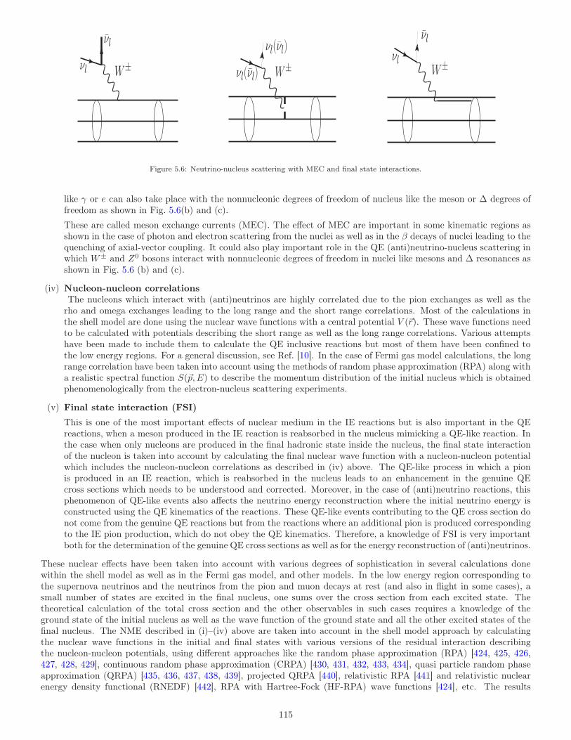
W±νl

νl

W±νl

νl

νl(νl)

νl(νl)

W±

Figure 5.6: Neutrino-nucleus scattering with MEC and final state interactions.

like γ or e can also take place with the nonnucleonic degrees of freedom of nucleus like the meson or ∆ degrees offreedom as shown in Fig. 5.6(b) and (c).

These are called meson exchange currents (MEC). The effect of MEC are important in some kinematic regions asshown in the case of photon and electron scattering from the nuclei as well as in the β decays of nuclei leading to thequenching of axial-vector coupling. It could also play important role in the QE (anti)neutrino-nucleus scattering inwhich W± and Z0 bosons interact with nonnucleonic degrees of freedom in nuclei like mesons and ∆ resonances asshown in Fig. 5.6 (b) and (c).

(iv) Nucleon-nucleon correlationsThe nucleons which interact with (anti)neutrinos are highly correlated due to the pion exchanges as well as the

rho and omega exchanges leading to the long range and the short range correlations. Most of the calculations inthe shell model are done using the nuclear wave functions with a central potential V (~r). These wave functions needto be calculated with potentials describing the short range as well as the long range correlations. Various attemptshave been made to include them to calculate the QE inclusive reactions but most of them have been confined tothe low energy regions. For a general discussion, see Ref. [10]. In the case of Fermi gas model calculations, the longrange correlation have been taken into account using the methods of random phase approximation (RPA) along witha realistic spectral function S(~p,E) to describe the momentum distribution of the initial nucleus which is obtainedphenomenologically from the electron-nucleus scattering experiments.

(v) Final state interaction (FSI)

This is one of the most important effects of nuclear medium in the IE reactions but is also important in the QEreactions, when a meson produced in the IE reaction is reabsorbed in the nucleus mimicking a QE-like reaction. Inthe case when only nucleons are produced in the final hadronic state inside the nucleus, the final state interactionof the nucleon is taken into account by calculating the final nuclear wave function with a nucleon-nucleon potentialwhich includes the nucleon-nucleon correlations as described in (iv) above. The QE-like process in which a pionis produced in an IE reaction, which is reabsorbed in the nucleus leads to an enhancement in the genuine QEcross sections which needs to be understood and corrected. Moreover, in the case of (anti)neutrino reactions, thisphenomenon of QE-like events also affects the neutrino energy reconstruction where the initial neutrino energy isconstructed using the QE kinematics of the reactions. These QE-like events contributing to the QE cross section donot come from the genuine QE reactions but from the reactions where an additional pion is produced correspondingto the IE pion production, which do not obey the QE kinematics. Therefore, a knowledge of FSI is very importantboth for the determination of the genuine QE cross sections as well as for the energy reconstruction of (anti)neutrinos.

These nuclear effects have been taken into account with various degrees of sophistication in several calculations donewithin the shell model as well as in the Fermi gas model, and other models. In the low energy region corresponding tothe supernova neutrinos and the neutrinos from the pion and muon decays at rest (and also in flight in some cases), asmall number of states are excited in the final nucleus, one sums over the cross section from each excited state. Thetheoretical calculation of the total cross section and the other observables in such cases requires a knowledge of theground state of the initial nucleus as well as the wave function of the ground state and all the other excited states of thefinal nucleus. The NME described in (i)–(iv) above are taken into account in the shell model approach by calculatingthe nuclear wave functions in the initial and final states with various versions of the residual interaction describingthe nucleon-nucleon potentials, using different approaches like the random phase approximation (RPA) [424, 425, 426,427, 428, 429], continuous random phase approximation (CRPA) [430, 431, 432, 433, 434], quasi particle random phaseapproximation (QRPA) [435, 436, 437, 438, 439], projected QRPA [440], relativistic RPA [441] and relativistic nuclearenergy density functional (RNEDF) [442], RPA with Hartree-Fock (HF-RPA) wave functions [424], etc. The results

115

obtained in these approaches have been reviewed by Kolbe et al. [443], and recently by Balasi et al. [444], and Jachowiczand Nikolakopoulos [445]. Alternate approaches, using the relativistic distorted wave impulse approximation (RDWIA)methods using relativistic mean fields as well as the Green’s function approaches using the nucleon-nucleon optical modelto describe the final state interactions of the nucleons have been used by the Spanish-Italian groups [446, 447, 448, 449].In recent years, the methods of SuperScaling Approach (SuSA) based on the scaling behavior of the nuclear responsefunctions observed in the electron-nucleus scattering has been applied to study the QE (anti)neutrino-nucleus scatteringby the MIT-Spanish-Italian groups [450, 451].

In the case of light nuclei like 4He, 6Li and 12C, the ab initio calculations of the nuclear response functions based onthe Green’s function Monte Carlo methods have been used by the Argonne-Rome group [452, 453]. In these approaches,some authors have also calculated the effect of MEC. These microscopic methods were used to calculate the cross sectionsfor transitions to all the accessible states (ground and excited states) in the final nucleus and sum over them to obtainthe total cross section. These methods become quite intractable when (anti)neutrino energies approach the GeV regionin which case some approximation methods are used.

Historically, the approximation methods based on the Fermi gas model [454, 455, 456] and the closure approxima-tion with the shell model wave functions [149, 457], which have been used to analyze the early (anti)neutrino-nucleusexperiments from CERN, ANL, and BNL laboratories. In view of the recent experiments in the few GeV region doneat Fermilab, JPARC, and CERN, various improved versions of the Fermi gas model have been used. It is not possibleto summarize in this report, all the microscopic approaches based on the calculations of NME mentioned above and wefocus in the following only on the latest work done using the Fermi gas model to describe NME in (anti)neutrino-nucleusQE scattering. For details, see Ref. [10].

5.4.1. (Anti)neutrino-nucleus quasielastic scattering in Fermi gas models

The first application of the Fermi gas model to the (anti)neutrino-nucleus scattering results from CERN was done byBerman et al. [456] using the works of Gatto [454, 455], where the free nucleon differential cross section dσ

dQ2 is multiplied

by a factor(

1− DN

)

and D is given by [149, 405, 456]:

D = Z for x < u− v

=1

2A

1− 3x

4(u2 + v2) +

x3

2− 3

32x(u2 − v2)2

for u− v < x < u+ v

= 0 for x > u+ v (5.63)

with x = |~q|2pF

, u = (2NA )1/3, v = (2ZA )1/3 and N(= A − Z), Z, A are neutron, proton and mass numbers of the initial

nucleus, respectively. pF is the Fermi momentum and the three momentum transfer |~q| =√

q20 +Q2, Q2 = −q2 ≥ 0.Smith and Moniz [458] improved the Fermi gas model calculations and used the following expression for the double

differential cross section:

d2σ

dk′dΩl=

G2Fk

′2 cos2(12χ)

2π2M

W2 + [2W1 +m2

l

M2Wα] tan

2(1

2χ) + (Wβ +W8)m

2l /(MEl cos2(

1

2χ))

− 2W8/M tan(1

2χ) sec(

1

2χ)[−Q2 cos2(

1

2χ) + |~q|2 sin2(

1

2χ) +m2

l ]12

, (5.64)

where cosχ = k′

Elcos θ. The form of Wi’s and other details are given in Ref. [458].

Gaisser and O’Connell [459] have used the relativistic response function R(~q, q0), in a Fermi gas model to take intoaccount NME. The expression for the double differential scattering cross section is given by

d2σ

dΩldEl= C

dσfreedΩl

R(~q, q0),

R(~q, q0) =1

43πp

3FN

∫

d3pN M2

ENEN ′

δ(EN + q0 − EB − EN ′)θ(pFN− |~pN |)θ(|~pN + ~q| − pFN′ ), (5.65)

where pFNis the Fermi momentum for the initial nucleon, N,N ′=n or p and C = A − Z for neutrino induced process

and C = Z for the antineutrino induced process.dσfree

dΩlis the differential scattering cross section for the (anti)neutrino

reaction on free (proton) neutron target.In 1990’s, the local Fermi gas model (LFGM) was used to study the (anti)neutrino-nucleus scattering in the low as well

as the intermediate energy region to study NME on the cross sections and possible modification of the axial dipole massMA due to NME [425, 427, 460]. In recent years, LFGM has been improved by taking into account the relativistic effects,the effects of long range nucleon-nucleon correlations and the use of a realistic spectral function S(~p,E) to describe thenucleon momentum distribution instead of a step function in momentum space used in the earlier calculations [461, 462].

116

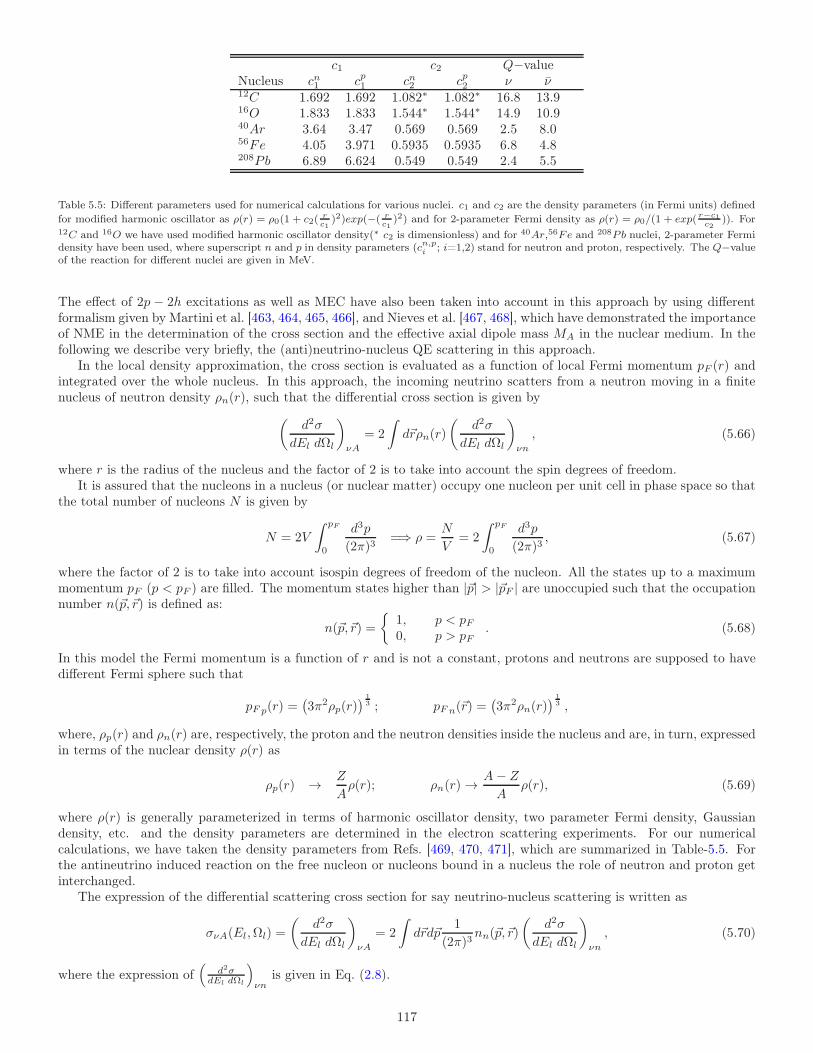
c1 c2 Q−valueNucleus cn1 cp1 cn2 cp2 ν ν12C 1.692 1.692 1.082∗ 1.082∗ 16.8 13.916O 1.833 1.833 1.544∗ 1.544∗ 14.9 10.940Ar 3.64 3.47 0.569 0.569 2.5 8.056Fe 4.05 3.971 0.5935 0.5935 6.8 4.8208Pb 6.89 6.624 0.549 0.549 2.4 5.5

Table 5.5: Different parameters used for numerical calculations for various nuclei. c1 and c2 are the density parameters (in Fermi units) defined

for modified harmonic oscillator as ρ(r) = ρ0(1 + c2(rc1

)2)exp(−( rc1

)2) and for 2-parameter Fermi density as ρ(r) = ρ0/(1 + exp( r−c1c2

)). For12C and 16O we have used modified harmonic oscillator density(∗ c2 is dimensionless) and for 40Ar,56Fe and 208Pb nuclei, 2-parameter Fermidensity have been used, where superscript n and p in density parameters (cn,p

i ; i=1,2) stand for neutron and proton, respectively. The Q−valueof the reaction for different nuclei are given in MeV.

The effect of 2p − 2h excitations as well as MEC have also been taken into account in this approach by using differentformalism given by Martini et al. [463, 464, 465, 466], and Nieves et al. [467, 468], which have demonstrated the importanceof NME in the determination of the cross section and the effective axial dipole mass MA in the nuclear medium. In thefollowing we describe very briefly, the (anti)neutrino-nucleus QE scattering in this approach.

In the local density approximation, the cross section is evaluated as a function of local Fermi momentum pF (r) andintegrated over the whole nucleus. In this approach, the incoming neutrino scatters from a neutron moving in a finitenucleus of neutron density ρn(r), such that the differential cross section is given by

(

d2σ

dEl dΩl

)

νA

= 2

∫

d~rρn(r)

(

d2σ

dEl dΩl

)

νn

, (5.66)

where r is the radius of the nucleus and the factor of 2 is to take into account the spin degrees of freedom.It is assured that the nucleons in a nucleus (or nuclear matter) occupy one nucleon per unit cell in phase space so that

the total number of nucleons N is given by

N = 2V

∫ pF

0

d3p

(2π)3=⇒ ρ =

N

V= 2

∫ pF

0

d3p

(2π)3, (5.67)

where the factor of 2 is to take into account isospin degrees of freedom of the nucleon. All the states up to a maximummomentum pF (p < pF ) are filled. The momentum states higher than |~p| > |~pF | are unoccupied such that the occupationnumber n(~p,~r) is defined as:

n(~p,~r) =

1, p < pF0, p > pF

. (5.68)

In this model the Fermi momentum is a function of r and is not a constant, protons and neutrons are supposed to havedifferent Fermi sphere such that

pF p(r) =(

3π2ρp(r))

13 ; pF n(~r) =

(

3π2ρn(r))

13 ,

where, ρp(r) and ρn(r) are, respectively, the proton and the neutron densities inside the nucleus and are, in turn, expressedin terms of the nuclear density ρ(r) as

ρp(r) → Z

Aρ(r); ρn(r)→

A− ZA

ρ(r), (5.69)

where ρ(r) is generally parameterized in terms of harmonic oscillator density, two parameter Fermi density, Gaussiandensity, etc. and the density parameters are determined in the electron scattering experiments. For our numericalcalculations, we have taken the density parameters from Refs. [469, 470, 471], which are summarized in Table-5.5. Forthe antineutrino induced reaction on the free nucleon or nucleons bound in a nucleus the role of neutron and proton getinterchanged.

The expression of the differential scattering cross section for say neutrino-nucleus scattering is written as

σνA(El,Ωl) =

(

d2σ

dEl dΩl

)

νA

= 2

∫

d~rd~p1

(2π)3nn(~p,~r)

(

d2σ

dEl dΩl

)

νn

, (5.70)

where the expression of(

d2σdEl dΩl

)

νnis given in Eq. (2.8).

117

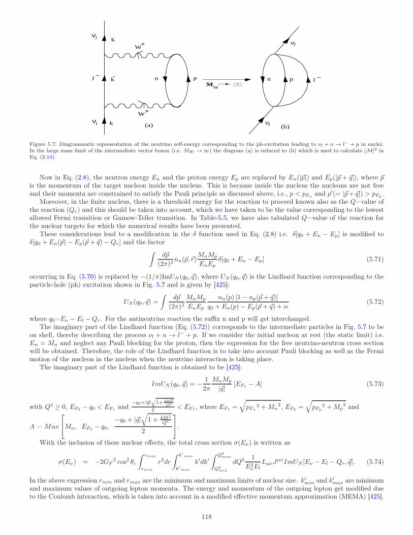
l

l k

k

W

W

n pl k_

MW

ν

ν

l_

n p

ν

ν

l

l+

+

(a) (b)

Figure 5.7: Diagrammatic representation of the neutrino self-energy corresponding to the ph-excitation leading to νl + n → l− + p in nuclei.In the large mass limit of the intermediate vector boson (i.e. MW → ∞) the diagram (a) is reduced to (b) which is used to calculate |M|2 inEq. (2.14).

Now in Eq. (2.8), the neutron energy En and the proton energy Ep are replaced by En(|~p|) and Ep(|~p+ ~q|), where ~pis the momentum of the target nucleon inside the nucleus. This is because inside the nucleus the nucleons are not freeand their momenta are constrained to satisfy the Pauli principle as discussed above, i.e., p < pFn

and p′(= |~p+ ~q|) > pFp.

Moreover, in the finite nucleus, there is a threshold energy for the reaction to proceed known also as the Q−value ofthe reaction (Qr) and this should be taken into account, which we have taken to be the value corresponding to the lowestallowed Fermi transition or Gamow-Teller transition. In Table-5.5, we have also tabulated Q−value of the reaction forthe nuclear targets for which the numerical results have been presented.

These considerations lead to a modification in the δ function used in Eq. (2.8) i.e. δ[q0 + En − Ep] is modified toδ[q0 + En(~p)− Ep(~p+ ~q)−Qr] and the factor

∫

d~p

(2π)3nn(~p,~r)

MnMp

EnEpδ[q0 + En − Ep] (5.71)

occurring in Eq. (5.70) is replaced by −(1/π)ImUN(q0, ~q), where UN (q0, ~q) is the Lindhard function corresponding to theparticle-hole (ph) excitation shown in Fig. 5.7 and is given by [425]:

UN(q0, ~q) =

∫

d~p

(2π)3MnMp

EnEp

nn(p) [1− np(~p+ ~q)]

q0 + En(p)− Ep(~p+ ~q) + iǫ(5.72)

where q0=Eν − El −Qr. For the antineutrino reaction the suffix n and p will get interchanged.The imaginary part of the Lindhard function (Eq. (5.72)) corresponds to the intermediate particles in Fig. 5.7 to be

on shell, thereby describing the process νl + n → l− + p. If we consider the initial nucleon at rest (the static limit) i.e.En = Mn and neglect any Pauli blocking for the proton, then the expression for the free neutrino-neutron cross sectionwill be obtained. Therefore, the role of the Lindhard function is to take into account Pauli blocking as well as the Fermimotion of the nucleon in the nucleus when the neutrino interaction is taking place.

The imaginary part of the Lindhard function is obtained to be [425]:

ImUN(q0, ~q) = −1

2π

MnMp

|~q| [EF1 −A] (5.73)

with Q2 ≥ 0, EF2 − q0 < EF1 and−q0+|~q|

√

1+ 4M2

Q2

2 < EF1 , where EF1 =√

pFn2 +Mn

2, EF2 =√

pFp2 +Mp

2 and

A = Max

Mn, EF2 − q0,−q0 + |~q|

√

1 + 4M2

Q2

2

.

With the inclusion of these nuclear effects, the total cross section σ(Eν) is written as

σ(Eν) = −2GF2 cos2 θc

∫ rmax

rmin

r2dr

∫ k′max

k′min

k′dk′∫ Q2

max

Q2min

dQ2 1

E2νEl

LµνJµνImUN [Eν − El −Qr, ~q]. (5.74)

In the above expression rmin and rmax are the minimum and maximum limits of nuclear size. k′min and k′max are minimumand maximum values of outgoing lepton momenta. The energy and momentum of the outgoing lepton get modified dueto the Coulomb interaction, which is taken into account in a modified effective momentum approximation (MEMA) [425].

118

+ + +.............. +..............

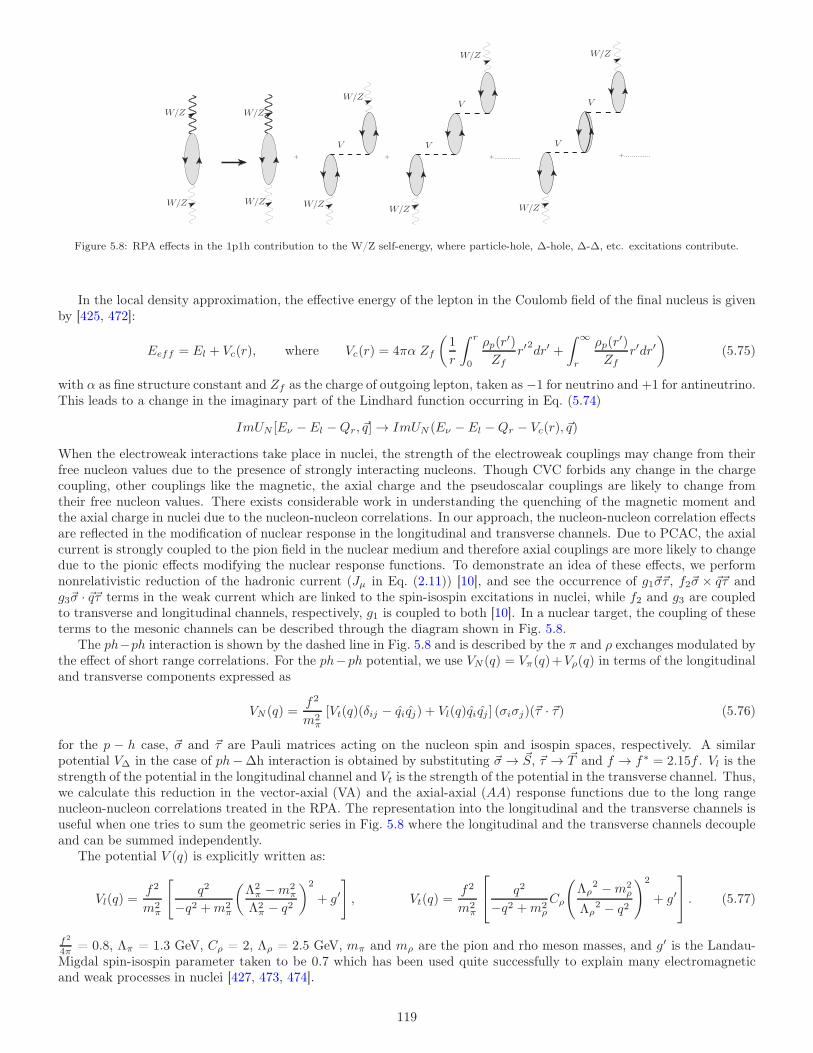
W/Z

W/Z W/Z

W/Z

W/Z

W/ZW/Z

W/Z

W/Z

W/Z

V V

V

V

V

Figure 5.8: RPA effects in the 1p1h contribution to the W/Z self-energy, where particle-hole, ∆-hole, ∆-∆, etc. excitations contribute.

In the local density approximation, the effective energy of the lepton in the Coulomb field of the final nucleus is givenby [425, 472]:

Eeff = El + Vc(r), where Vc(r) = 4πα Zf

(

1

r

∫ r

0

ρp(r′)

Zfr′

2dr′ +

∫ ∞

r

ρp(r′)

Zfr′dr′

)

(5.75)

with α as fine structure constant and Zf as the charge of outgoing lepton, taken as −1 for neutrino and +1 for antineutrino.This leads to a change in the imaginary part of the Lindhard function occurring in Eq. (5.74)

ImUN [Eν − El −Qr, ~q]→ ImUN (Eν − El −Qr − Vc(r), ~q)

When the electroweak interactions take place in nuclei, the strength of the electroweak couplings may change from theirfree nucleon values due to the presence of strongly interacting nucleons. Though CVC forbids any change in the chargecoupling, other couplings like the magnetic, the axial charge and the pseudoscalar couplings are likely to change fromtheir free nucleon values. There exists considerable work in understanding the quenching of the magnetic moment andthe axial charge in nuclei due to the nucleon-nucleon correlations. In our approach, the nucleon-nucleon correlation effectsare reflected in the modification of nuclear response in the longitudinal and transverse channels. Due to PCAC, the axialcurrent is strongly coupled to the pion field in the nuclear medium and therefore axial couplings are more likely to changedue to the pionic effects modifying the nuclear response functions. To demonstrate an idea of these effects, we performnonrelativistic reduction of the hadronic current (Jµ in Eq. (2.11)) [10], and see the occurrence of g1~σ~τ , f2~σ × ~q~τ andg3~σ · ~q~τ terms in the weak current which are linked to the spin-isospin excitations in nuclei, while f2 and g3 are coupledto transverse and longitudinal channels, respectively, g1 is coupled to both [10]. In a nuclear target, the coupling of theseterms to the mesonic channels can be described through the diagram shown in Fig. 5.8.

The ph−ph interaction is shown by the dashed line in Fig. 5.8 and is described by the π and ρ exchanges modulated bythe effect of short range correlations. For the ph−ph potential, we use VN (q) = Vπ(q)+Vρ(q) in terms of the longitudinaland transverse components expressed as

VN (q) =f2

m2π

[Vt(q)(δij − qiqj) + Vl(q)qiqj ] (σiσj)(~τ · ~τ) (5.76)

for the p − h case, ~σ and ~τ are Pauli matrices acting on the nucleon spin and isospin spaces, respectively. A similarpotential V∆ in the case of ph−∆h interaction is obtained by substituting ~σ → ~S, ~τ → ~T and f → f∗ = 2.15f . Vl is thestrength of the potential in the longitudinal channel and Vt is the strength of the potential in the transverse channel. Thus,we calculate this reduction in the vector-axial (VA) and the axial-axial (AA) response functions due to the long rangenucleon-nucleon correlations treated in the RPA. The representation into the longitudinal and the transverse channels isuseful when one tries to sum the geometric series in Fig. 5.8 where the longitudinal and the transverse channels decoupleand can be summed independently.

The potential V (q) is explicitly written as:

Vl(q) =f2

m2π

[

q2

−q2 +m2π

(

Λ2π −m2

π

Λ2π − q2

)2

+ g′]

, Vt(q) =f2

m2π

q2

−q2 +m2ρ

Cρ

(

Λρ2 −m2

ρ

Λρ2 − q2

)2

+ g′

. (5.77)

f2

4π = 0.8, Λπ = 1.3 GeV, Cρ = 2, Λρ = 2.5 GeV, mπ and mρ are the pion and rho meson masses, and g′ is the Landau-Migdal spin-isospin parameter taken to be 0.7 which has been used quite successfully to explain many electromagneticand weak processes in nuclei [427, 473, 474].

119

Using the matrix elements at the weak WNN vertex and the ph− ph potential, the contribution of Fig. 5.8 is writtenas

U(q) = U(q) + U(q)VN (q)U(q) + U(q)VN (q)U(q)VN (q)U(q) + ... (5.78)

Writing the potential VN (q) in terms of Vl and Vt, the above series can be separated in the longitudinal and the transversecomponents. The longitudinal component is then written as [10]:

UL(q) =

[

U(q)

1− U(q)Vl

]

qiqj σiσj ~τ1 · ~τ2. (5.79)

Similarly, the transverse component is given by [10]:

UT (q) =

[

U(q)

1− U(q)Vt

]

(δij − qiqj) σiσj ~τ1 · ~τ2. (5.80)

Therefore, we can write Eq. (5.78) as:

U(q)→ U(q) =

[(

U(q)

1− U(q)Vt

)

(δij − qiqj) +(

U(q)

1− U(q)Vl

)

qiqj

]

~σi ~σj ~τ1 · ~τ2, (5.81)

where U = UN+U∆, with UN and U∆ as the Lindhard function for p−h and ∆−h excitations, respectively, in the mediumand the expressions for UN and U∆ are taken from Ref. [475, 476]. The different couplings of N and ∆ are incorporatedin UN and U∆ and then the same interaction strengths Vl(q) and Vt(q) are used to calculate the RPA response. Theseeffects have been discussed by Nieves et al. [477] as well as by Athar et al. [478].

By using the above method of renormalization, we consider the different components of the hadronic tensor Jµν (Eq. (2.16))and sum up the RPA series shown in Fig. 5.8. For convenience we take ~q to be along the z direction and neglect all the

corrections of order O(

kF ~pM2 ,

kF ~p′

M2 ,kF q0M2

)

, and the different components of Jµν like J00, J0z, Jzz, etc. with renormalization

effect are obtained as [477, 478]:

JRPA00

M2=

(

f1(Q2))2

[

(

E(~p)

M

)2

+

(

q0E(~p)−Q2/4

M2

)

]

+Q2

M2

(

f2(Q2)

2

)2 [~p2 + q0E(~p) + q20/4

M2− q20Q2

]

− 1

2

(

f1(Q2)f2(Q

2))

( |~q|M

)2

+ g21(Q2)

[

~p2 + q0E(~p)−Q2/4

M2+ UL

(

q20m2

π +Q2

)(

Q2

m2π +Q2

)]

(5.82)

JRPA0z

M2=

1

2

(

f1(Q2))2[

E(~p)

M

(

2pz + |~q|M

)

+qopzM2

]

+1

2

Q2

M2

(

f2(Q2)

2

)2 [E(~p)

M

(

2pz + |~q|M

)

− 2q0|~q|Q2

+q0 (2pz + |~q|)

2M2

]

− 1

2

(

f1(Q2)f2(Q

2))

[

q0|~q|M2

]

+ g21(Q2)

[

ULE(~p)

M

(

2pz + |~q|2M

)

+qopz2M2

+ UL

(

q0|~q|m2

π +Q2

)(

q2

m2π +Q2

)]

(5.83)

JRPAzz

M2=

(

f1(Q2))2[

p2z + |~q|pz +Q2/4

M2

]

+1

4

Q2

M2

(

f2(Q2)

2

)2[

(

2pz + |~q|M

)2

− q20Q2

]

− 1

2

(

f1(Q2)f2(Q

2))

( q0M

)2

+ g21(Q2)

[

UL +p2z + |~q|pz +Q2/4

M2+ UL

( |~q|m2

π +Q2

)(

Q2

m2π +Q2

)]

(5.84)

JxxRPA

M2=

(

f1(Q2))2[

p2x +Q2/4

M2

]

+Q2

M2

(

f2(Q2)

2

)2 [

UT +p2xM2

]

+1

2

(

f1(Q2)f2(Q

2))

UT

(

Q2

M2

)

+ g21(Q2)

[

UL +p2x +Q2/4

M2

]

(5.85)

JRPAxy

M2= ig1(Q

2)[

f1(Q2) + f2(Q

2)]

[

q0pzM2

− UT|~q|E(~p)

M2

]

. (5.86)

Thus, in a local density approximation in the presence of NME including the RPA effect, the total cross section σ(Eν ),is written as

σ(Eν ) = −2GF2 cos2 θc

∫ rmax

rmin

r2dr

∫ k′max

k′min

k′dk′∫ Q2

max

Q2min

dQ2 1

E2νEl

LµνJµνRPAImUN [Eν − El −Qr − Vc(r), ~q] (5.87)

where JµνRPA is the modified hadronic tensor when RPA effect is incorporated and the energy transferred to the hadronic

tensor also gets modified from q0 = Eν − El to q0 = Eν − El −Qr − Vc.

120

5.4.2. Inclusive quasielastic scattering at low energy

5.4.3.1 Theoretical results and comparison with experimentsWe summarize in this section, the experimental and theoretical results for the low energy inclusive (νe, e

−), (νµ, µ−)scattering cross sections from the KARMEN and LSND collaborations in 12C, presented in Table-5.6 [424, 425, 426,427, 428, 431, 443, 477, 478, 479, 480, 481, 482, 483, 484, 485, 486, 487, 488, 489, 490, 491, 492, 493], along withthe theoretical predictions for these processes in various nuclear models. Most of the theoretical methods used toobtain these results were earlier developed to study the related process of the inclusive muon capture for which theresults are also included in Table 5.6. We have included theoretical results only from those calculations which quoteresults for the relevant physical observable for all the three processes i.e. the total cross section for the (νe, e

−) and(νµ, µ

−) inclusive scattering as well as the total rates for muon capture in 12C using the same nuclear model.

The various microscopic nuclear models referred in the column 3 of Table-5.6, in general use the shell model withvarying model spaces including states from 1 ~ω to 4 ~ω excitations to calculate the ground state of the initial aswell as the ground state and excited states of the final nuclei and transitions between them. The various modelsuse different forms of the phenomenological nucleon-nucleon potential like the Bonn potential, Landau-Migdalpotential or the Skymre model potential to calculate the nuclear states. Moreover, the residual interaction betweenthe nucleons which leads to the pairing and also to the quasi-particle excitations of nucleons in the nuclei arealso included in some nuclear models to calculate the nuclear wave functions of the higher excited states and thecontinuum state in the final nucleus. Depending upon the various assumptions and approximations, many nuclearmodels have been used to calculate the total cross sections for (νe e−) and (νµ µ−) reactions as well as the inclusivemuon capture rates. The results for the inclusive cross sections, and muon capture rates from these calculations areshown in Table-5.6, column-3. In column-4, we show the results for these observables obtained in various versions ofthe Fermi gas models. It should be noted that the different entries for the total cross sections or the capture ratesquoted under the same reference in column-3 and 4 of Table-5.6 corresponds to the various versions of the nuclearmodels and the parameters used in that model.

The following general observations about the theoretical results and their comparisons with the experimental resultsshown here in Table 5.6, can be made:

(i) There is no microscopic nuclear model, which is able to explain all the three weak processes involving νe, νµand muon capture. Even in a given model by changing the parameters of the model i.e. the various versionsof the model, it is possible to explain either the cross section for the inclusive QE reactions or the inclusivemuon capture but not both of them simultaneously [424, 428, 431, 443, 479, 483, 484, 487, 488, 489, 490, 493].

(ii) In the case of LFGM also the earlier nonrelativistic calculations by Singh and Oset [425, 427], Umino etal. [485, 486], Kosmas and Oset [426], Nieves et al. [477], and Athar et al. [478], in LFGM including RPAreproduce (νe, e

−) but overestimate the (νµ, µ−) reaction cross section and underestimate (µ−, νµ) capture

rate. The LFGM has been considerably improved in the latest calculations by Nieves and Sobczyk [481],where relativistic transition operators and the spectral function of nucleons are used to calculate all the threeprocesses. These models reproduce (νe, e

−) and (νµ, µ−) inclusive cross sections quite well but underestimate

the inclusive (µ−, νµ) capture rates.

In summary, a satisfactory understanding of the nuclear reactions with νµ, νe scattering, and µ capture in nucleartargets in the energy region of E < 230 MeV is desirable.

5.4.3.2 Inclusive cross sections with monoenergetic KDAR neutrinos with Eνµ = 236 MeVThe monoenergetic muon neutrinos from KDAR are identified as an ideal probe to study the neutrino-nucleus crosssections in the low energy region in order to benchmark NME in the exclusive as well as in the inclusive reactions inthis energy region. An experiment for measuring neutrino cross section σ(Eνµ ) with monoenergetic neutrinos wouldbe free from the uncertainties arising from the reconstruction procedure of the initial neutrino energy present inmost of the present experiments using beams of continuous energy of the muon neutrinos from accelerators. Somenew experiments have been planned to measure inclusive cross sections in 12C and 40Ar using the monoenergeticneutrinos from kaons decaying at rest. The monoenergetic neutrinos from kaons decaying at rest K+ → µ+νµ arecopiously produced with an energy Eνµ = 236 MeV, along with a continuous energy spectrum of νe and νµ fromKl3 decays like K+ → π0e+νe and K+ → π0µ+νµ.

The first measurements of the inclusive cross section in 12C nucleus with the monoenergetic KDAR muon neutrinoshas been recently reported by the MiniBooNE collaboration to be σ = (2.7± 1.2)× 10−39 cm2 [494]. Theoretically,this reaction in 12C in the energy region of few hundreds of MeV, has been studied by many authors, but specificcalculations and discussions of the inclusive cross section for Eνµ = 236 MeV have been done recently by Akbar etal. [495] in the relativistic Fermi gas model with RPA to include the effect of correlations and Nikolakopoulos etal. [496] in a microscopic model using CRPA to include the effect of nucleon-nucleon correlations. Nikolakopoulos

121

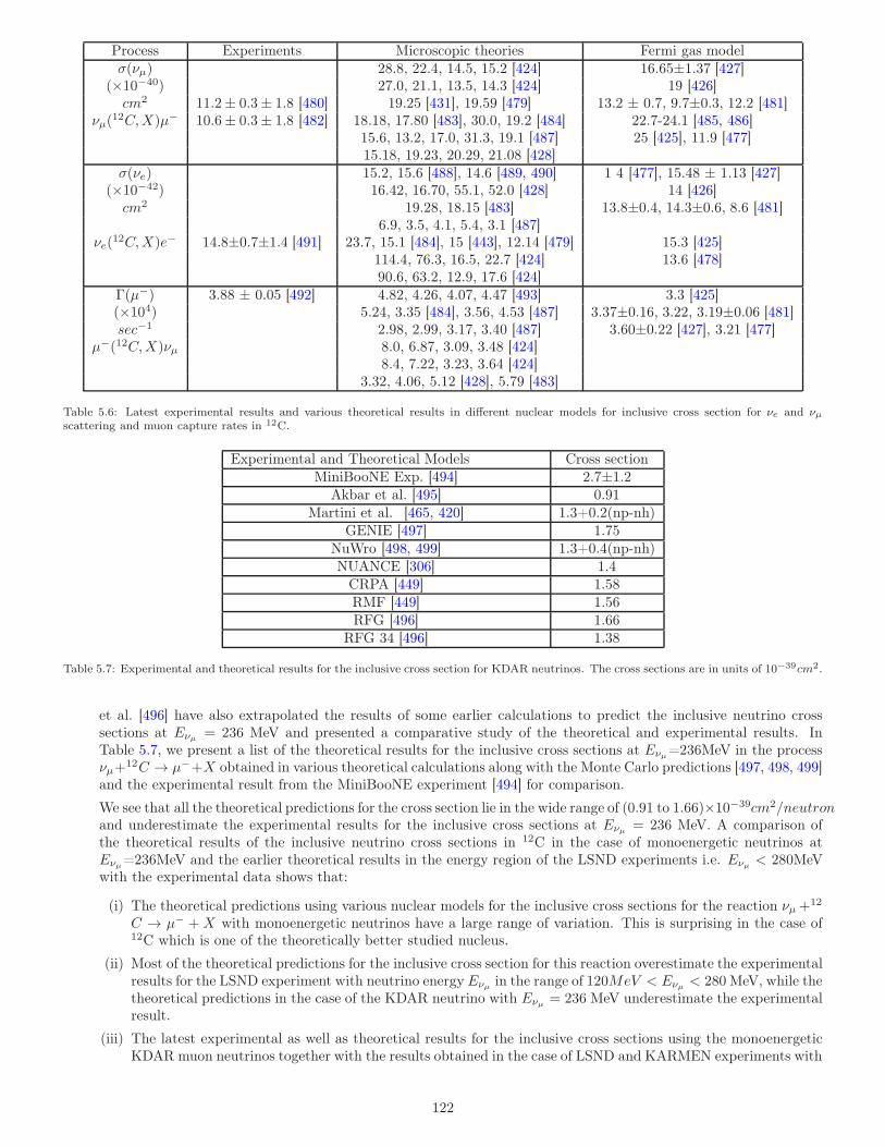
Process Experiments Microscopic theories Fermi gas modelσ(νµ) 28.8, 22.4, 14.5, 15.2 [424] 16.65±1.37 [427]

(×10−40) 27.0, 21.1, 13.5, 14.3 [424] 19 [426]cm2 11.2± 0.3± 1.8 [480] 19.25 [431], 19.59 [479] 13.2 ± 0.7, 9.7±0.3, 12.2 [481]

νµ(12C,X)µ− 10.6± 0.3± 1.8 [482] 18.18, 17.80 [483], 30.0, 19.2 [484] 22.7-24.1 [485, 486]

15.6, 13.2, 17.0, 31.3, 19.1 [487] 25 [425], 11.9 [477]15.18, 19.23, 20.29, 21.08 [428]

σ(νe) 15.2, 15.6 [488], 14.6 [489, 490] 1 4 [477], 15.48 ± 1.13 [427](×10−42) 16.42, 16.70, 55.1, 52.0 [428] 14 [426]cm2 19.28, 18.15 [483] 13.8±0.4, 14.3±0.6, 8.6 [481]

6.9, 3.5, 4.1, 5.4, 3.1 [487]νe(

12C,X)e− 14.8±0.7±1.4 [491] 23.7, 15.1 [484], 15 [443], 12.14 [479] 15.3 [425]114.4, 76.3, 16.5, 22.7 [424] 13.6 [478]90.6, 63.2, 12.9, 17.6 [424]

Γ(µ−) 3.88 ± 0.05 [492] 4.82, 4.26, 4.07, 4.47 [493] 3.3 [425](×104) 5.24, 3.35 [484], 3.56, 4.53 [487] 3.37±0.16, 3.22, 3.19±0.06 [481]sec−1 2.98, 2.99, 3.17, 3.40 [487] 3.60±0.22 [427], 3.21 [477]

µ−(12C,X)νµ 8.0, 6.87, 3.09, 3.48 [424]8.4, 7.22, 3.23, 3.64 [424]

3.32, 4.06, 5.12 [428], 5.79 [483]

Table 5.6: Latest experimental results and various theoretical results in different nuclear models for inclusive cross section for νe and νµscattering and muon capture rates in 12C.

Experimental and Theoretical Models Cross sectionMiniBooNE Exp. [494] 2.7±1.2

Akbar et al. [495] 0.91Martini et al. [465, 420] 1.3+0.2(np-nh)

GENIE [497] 1.75NuWro [498, 499] 1.3+0.4(np-nh)NUANCE [306] 1.4

CRPA [449] 1.58RMF [449] 1.56RFG [496] 1.66

RFG 34 [496] 1.38

Table 5.7: Experimental and theoretical results for the inclusive cross section for KDAR neutrinos. The cross sections are in units of 10−39cm2.

et al. [496] have also extrapolated the results of some earlier calculations to predict the inclusive neutrino crosssections at Eνµ = 236 MeV and presented a comparative study of the theoretical and experimental results. InTable 5.7, we present a list of the theoretical results for the inclusive cross sections at Eνµ=236MeV in the processνµ+

12C → µ−+X obtained in various theoretical calculations along with the Monte Carlo predictions [497, 498, 499]and the experimental result from the MiniBooNE experiment [494] for comparison.

We see that all the theoretical predictions for the cross section lie in the wide range of (0.91 to 1.66)×10−39cm2/neutronand underestimate the experimental results for the inclusive cross sections at Eνµ = 236 MeV. A comparison ofthe theoretical results of the inclusive neutrino cross sections in 12C in the case of monoenergetic neutrinos atEνµ=236MeV and the earlier theoretical results in the energy region of the LSND experiments i.e. Eνµ < 280MeVwith the experimental data shows that:

(i) The theoretical predictions using various nuclear models for the inclusive cross sections for the reaction νµ +12

C → µ− +X with monoenergetic neutrinos have a large range of variation. This is surprising in the case of12C which is one of the theoretically better studied nucleus.

(ii) Most of the theoretical predictions for the inclusive cross section for this reaction overestimate the experimentalresults for the LSND experiment with neutrino energyEνµ in the range of 120MeV < Eνµ < 280 MeV, while thetheoretical predictions in the case of the KDAR neutrino with Eνµ = 236 MeV underestimate the experimentalresult.

(iii) The latest experimental as well as theoretical results for the inclusive cross sections using the monoenergeticKDAR muon neutrinos together with the results obtained in the case of LSND and KARMEN experiments with

122

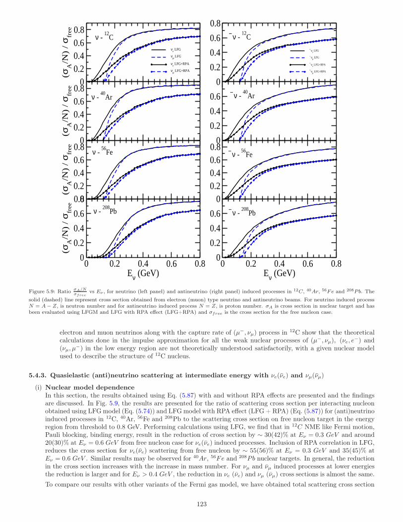
00.20.40.60.8

(σA

/N)

/ σ

free

νe LFG

νµ LFG

νe LFG+RPA

νµ LFG+RPA

0

0.2

0.4

0.6

0.8

νe LFG

ν µ LFG

νe LFG+RPA

ν µ LFG+RPA

00.20.40.60.8

(σA

/N)

/ σ

free

0

0.2

0.4

0.6

00.20.40.60.8

(σA

/N)

/ σ

free

00.20.40.60.8

0 0.2 0.4 0.6 0.8Eν (GeV)

0

0.2

0.4

0.6

0.8

(σA

/N)

/ σ

free

0 0.2 0.4 0.6 0.8Eν (GeV)

0

0.2

0.4

0.6

ν - 12

C

ν - 40

Ar

ν - 56

Fe

ν - 12

C

ν - 40

Ar

ν - 56

Fe

ν - 208

Pb ν - 208

Pb

Figure 5.9: Ratio σA/Nσfree

vs Eν , for neutrino (left panel) and antineutrino (right panel) induced processes in 12C, 40Ar, 56Fe and 208Pb. The

solid (dashed) line represent cross section obtained from electron (muon) type neutrino and antineutrino beams. For neutrino induced processN = A− Z, is neutron number and for antineutrino induced process N = Z, is proton number. σA is cross section in nuclear target and hasbeen evaluated using LFGM and LFG with RPA effect (LFG+RPA) and σfree is the cross section for the free nucleon case.

electron and muon neutrinos along with the capture rate of (µ−, νµ) process in 12C show that the theoreticalcalculations done in the impulse approximation for all the weak nuclear processes of (µ−, νµ), (νe, e

−) and(νµ, µ

−) in the low energy region are not theoretically understood satisfactorily, with a given nuclear modelused to describe the structure of 12C nucleus.

5.4.3. Quasielastic (anti)neutrino scattering at intermediate energy with νe(νe) and νµ(νµ)

(i) Nuclear model dependenceIn this section, the results obtained using Eq. (5.87) with and without RPA effects are presented and the findingsare discussed. In Fig. 5.9, the results are presented for the ratio of scattering cross section per interacting nucleonobtained using LFG model (Eq. (5.74)) and LFG model with RPA effect (LFG + RPA) (Eq. (5.87)) for (anti)neutrinoinduced processes in 12C, 40Ar, 56Fe and 208Pb to the scattering cross section on free nucleon target in the energyregion from threshold to 0.8 GeV. Performing calculations using LFG, we find that in 12C NME like Fermi motion,Pauli blocking, binding energy, result in the reduction of cross section by ∼ 30(42)% at Eν = 0.3 GeV and around20(30)% at Eν = 0.6 GeV from free nucleon case for νe(νe) induced processes. Inclusion of RPA correlation in LFG,reduces the cross section for νe(νe) scattering from free nucleon by ∼ 55(56)% at Eν = 0.3 GeV and 35(45)% atEν = 0.6 GeV . Similar results may be observed for 40Ar, 56Fe and 208Pb nuclear targets. In general, the reductionin the cross section increases with the increase in mass number. For νµ and νµ induced processes at lower energiesthe reduction is larger and for Eν > 0.4 GeV , the reduction in νe (νe) and νµ (νµ) cross sections is almost the same.

To compare our results with other variants of the Fermi gas model, we have obtained total scattering cross section

123

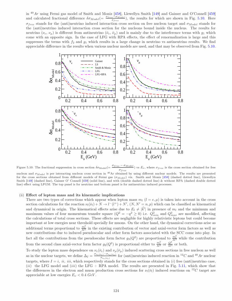
in 40Ar using Fermi gas model of Smith and Moniz [458], Llewellyn Smith [149] and Gaisser and O’Connell [459]and calculated fractional difference δσModel(=

σfree−σModel

σfree), the results for which are shown in Fig. 5.10. Here

σfree stands for the (anti)neutrino induced interaction cross section on free nucleon target and σModel stands forthe (anti)neutrino induced interaction cross section for the nucleons bound inside the nucleus. The results forneutrino (νe, νµ) is different from antineutrino (νe, νµ) and is mainly due to the interference terms with g1 whichcome with an opposite sign. In the case of LFG with RPA effects, the effect of renormalization is large and thissuppresses the terms with f2 and g1 which results in a large change in neutrino vs antineutrino results. We findappreciable difference in the results when various nuclear models are used, and that may be observed from Fig. 5.10.

0.2 0.4 0.6 0.80

0.2

0.4

0.6

0.8

1δσ

Mo

del

GaisserLSSmith & MonizLFGLFG+RPA

0.2 0.4 0.6 0.80

0.2

0.4

0.6

0.8

1

0.2 0.4 0.6 0.8Eν (GeV)

0

0.2

0.4

0.6

0.8

δσM

od

el

0.2 0.4 0.6 0.8Eν (GeV)

0

0.2

0.4

0.6

0.8

1

νe

νµ

νe ν µ

Figure 5.10: The fractional suppression in cross section δσModel(=σfree − σModel

σfree) vs Eν , where σfree is the cross section obtained for free

nucleon and σModel is per interacting nucleon cross section in 40Ar obtained by using different nuclear models. The results are presentedfor the cross sections obtained from different models of Fermi gas (σModel) viz. Smith and Moniz [458] (dashed dotted line), LlewellynSmith [149] (dashed line), Gaisser O’ Connell [459] (solid line), and with (double dashed dotted line) & without RPA (dashed double dottedline) effect using LFGM. The top panel is for neutrino and bottom panel is for antineutrino induced processes.

(ii) Effect of lepton mass and its kinematic implicationsThere are two types of corrections which appear when lepton mass ml (l = e, µ) is taken into account in the crosssection calculations for the reaction νl(νl)+N → l−(l+)+N ′, (N,N ′ = n, p) which can be classified as kinematical

and dynamical in origin. The kinematical effects arise due to El 6= |~k′| in presence of ml and the minimum andmaximum values of four momentum transfer square (Q2 = −q2 ≥ 0) i.e. Q2

min and Q2max are modified, affecting

the calculations of total cross sections. These effects are negligible for highly relativistic leptons but could becomeimportant at low energies near threshold specially for muons. On the other hand, the dynamical corrections arise as

additional terms proportional tom2

l

M2 in the existing contribution of vector and axial-vector form factors as well asnew contributions due to induced pseudoscalar and other form factors associated with the SCC come into play. In

fact all the contributions from the pseudoscalar form factor g3(Q2) are proportional to

m2l

M2 while the contribution

from the second class axial-vector form factor g2(Q2) is proportional either to

m2l

M2 or Q2

M2 or both.

To study the lepton mass dependence on νe(νe) and νµ(νµ) induced scattering cross sections in free nucleon as well

as in the nuclear targets, we define ∆I =σνe(νe)−σνµ(νµ)

σνe(νe)for (anti)neutrino induced reaction in 12C and 40Ar nuclear

targets, where I = i, ii, iii, which respectively stands for the cross sections obtained in (i) free (anti)neutrino case,(ii) the LFG model and (iii) the LFG + RPA model. The results are presented in Fig. 5.11, which show thatthe differences in the electron and muon production cross sections for νl(νl) induced reactions on 12C target areappreciable at low energies Eν < 0.4 GeV .

124

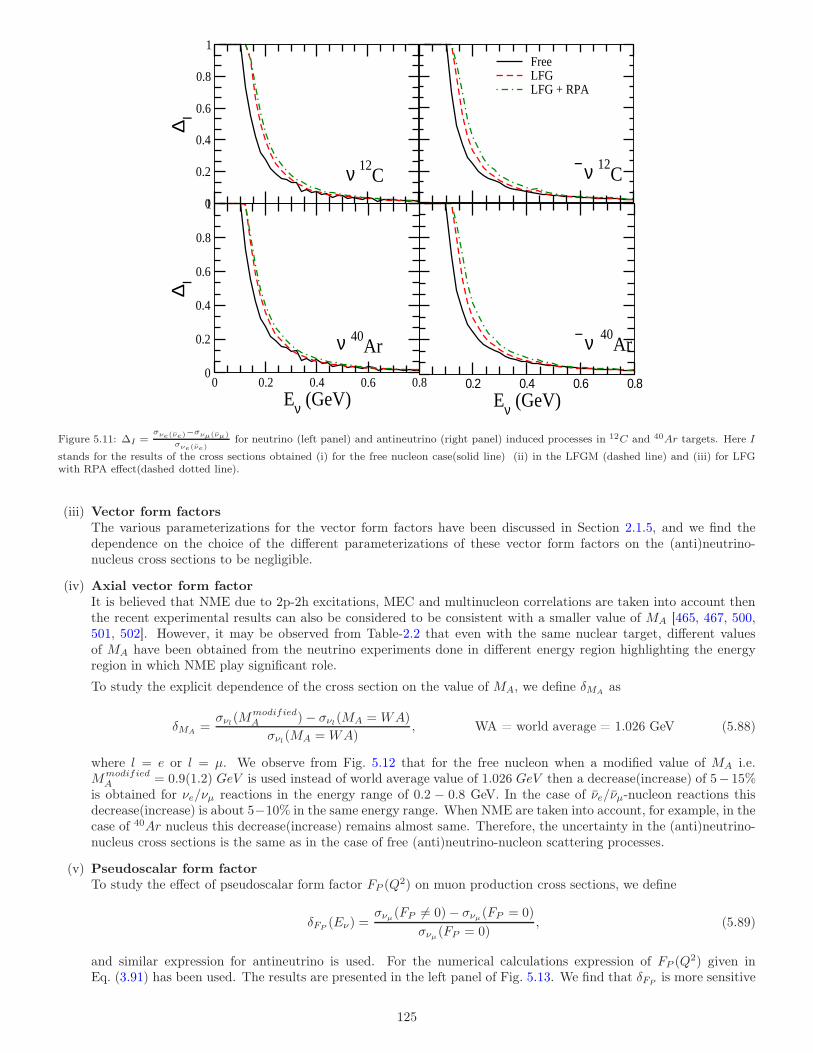
0

0.2

0.4

0.6

0.8

1

∆Ι

FreeLFGLFG + RPA

0 0.2 0.4 0.6 0.8

Eν (GeV)

0

0.2

0.4

0.6

0.8

1

∆Ι

0.2 0.4 0.6 0.8Eν (GeV)

ν 12C

ν ν40Ar

40Ar

12Cν

Figure 5.11: ∆I =σνe(νe)−σνµ(νµ)

σνe(νe)for neutrino (left panel) and antineutrino (right panel) induced processes in 12C and 40Ar targets. Here I

stands for the results of the cross sections obtained (i) for the free nucleon case(solid line) (ii) in the LFGM (dashed line) and (iii) for LFGwith RPA effect(dashed dotted line).

(iii) Vector form factorsThe various parameterizations for the vector form factors have been discussed in Section 2.1.5, and we find thedependence on the choice of the different parameterizations of these vector form factors on the (anti)neutrino-nucleus cross sections to be negligible.

(iv) Axial vector form factorIt is believed that NME due to 2p-2h excitations, MEC and multinucleon correlations are taken into account thenthe recent experimental results can also be considered to be consistent with a smaller value of MA [465, 467, 500,501, 502]. However, it may be observed from Table-2.2 that even with the same nuclear target, different valuesof MA have been obtained from the neutrino experiments done in different energy region highlighting the energyregion in which NME play significant role.

To study the explicit dependence of the cross section on the value of MA, we define δMAas

δMA=σνl(M

modifiedA )− σνl(MA =WA)

σνl(MA =WA), WA = world average = 1.026 GeV (5.88)

where l = e or l = µ. We observe from Fig. 5.12 that for the free nucleon when a modified value of MA i.e.Mmodified

A = 0.9(1.2) GeV is used instead of world average value of 1.026 GeV then a decrease(increase) of 5− 15%is obtained for νe/νµ reactions in the energy range of 0.2 − 0.8 GeV. In the case of νe/νµ-nucleon reactions thisdecrease(increase) is about 5−10% in the same energy range. When NME are taken into account, for example, in thecase of 40Ar nucleus this decrease(increase) remains almost same. Therefore, the uncertainty in the (anti)neutrino-nucleus cross sections is the same as in the case of free (anti)neutrino-nucleon scattering processes.

(v) Pseudoscalar form factorTo study the effect of pseudoscalar form factor FP (Q

2) on muon production cross sections, we define

δFP(Eν) =

σνµ(FP 6= 0)− σνµ(FP = 0)

σνµ(FP = 0), (5.89)

and similar expression for antineutrino is used. For the numerical calculations expression of FP (Q2) given in

Eq. (3.91) has been used. The results are presented in the left panel of Fig. 5.13. We find that δFPis more sensitive

125

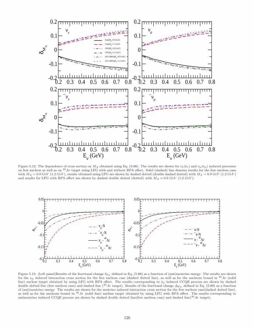
0.2 0.3 0.4 0.5 0.6 0.7 0.8-0.2

-0.1

0

0.1

0.2

δ MA

Free(MA

=0.9 GeV)

Free(MA

=1.2 GeV)

LFG(MA=0.9 GeV)

LFG(MA=1.2 GeV)

LFG+RPA(MA

=0.9 GeV)

LFG+RPA(MA

=1.2 GeV)

0.2 0.3 0.4 0.5 0.6 0.7 0.8-0.2

-0.1

0

0.1

0.2

0.2 0.3 0.4 0.5 0.6 0.7 0.8Eν (GeV)

-0.2

-0.1

0

0.1

0.2

δ MA

0.2 0.3 0.4 0.5 0.6 0.7 0.8Eν (GeV)

-0.2

-0.1

0

0.1

0.2

νe

νµ

νe ν µ

Figure 5.12: The dependence of cross section on MA obtained using Eq. (5.88). The results are shown for νe(νe) and νµ(νµ) induced processeson free nucleon as well as on 40Ar target using LFG with and without RPA effect. Solid (dashed) line denotes results for the free nucleon casewith MA = 0.9 GeV (1.2 GeV ), results obtained using LFG are shown by dashed dotted (double dashed dotted) with MA = 0.9 GeV (1.2 GeV )and results for LFG with RPA effect are shown by dashed double dotted (dotted) with MA = 0.9 GeV (1.2 GeV ).

0.2 0.3 0.4 0.5 0.6 0.7 0.8Eν (GeV)

-0.2

-0.15

-0.1

-0.05

0

0.05

δ FP νµ-N

ν µ-N

νµ - 40

Ar

ν µ - 40

Ar

0.2 0.3 0.4 0.5 0.6 0.7 0.8Eν (GeV)

-0.2

-0.15

-0.1

-0.05

0

0.05

∆F

P

ν-Nν -Nν -

40Ar

ν - 40

Ar

Figure 5.13: (Left panel)Results of the fractional change δFPdefined in Eq. (5.89) as a function of (anti)neutrino energy. The results are shown

for the νµ induced interaction cross section for the free nucleon case (dashed dotted line), as well as for the nucleons bound in 40Ar (solidline) nuclear target obtained by using LFG with RPA effect. The results corresponding to νµ induced CCQE process are shown by dasheddouble dotted line (free nucleon case) and dashed line (40Ar target). Results of the fractional change ∆FP

defined in Eq. (5.89) as a functionof (anti)neutrino energy. The results are shown for the neutrino induced interaction cross section for the free nucleon case(dashed dotted line),as well as for the nucleons bound in 40Ar (solid line) nuclear target obtained by using LFG with RPA effect. The results corresponding toantineutrino induced CCQE process are shown by dashed double dotted line(free nucleon case) and dashed line(40Ar target).

126

in the case of νµ induced CCQE process than νµ induced process for the free nucleon case as well as for 40Ar nucleartarget. This sensitivity decreases with the increase in νµ/νµ energy and almost vanishes beyond 0.6 GeV .

We also study the sensitivity of pseudoscalar form factor FP (Q2) to find out the difference in the electron vs muon

production cross sections that are obtained using Eq. (3.91). For this purpose we define

∆1(Eν) =σνµ (FP 6= 0)− σνe(FP 6= 0)

σνe(FP 6= 0); ∆2(Eν) =

σνµ(FP = 0)− σνe(FP = 0)

σνe(FP = 0); ∆FP

= ∆1(Eν)−∆2(Eν). (5.90)

and the results for ∆FPare shown in Fig. 5.13.

We have calculated the fractional difference ∆FPas given in Eq. (5.90) for free nucleon case as well as for nucleons

bound in 40Ar nuclear target using the LFG with RPA effect. We observe that the inclusion of pseudoscalar formfactor decreases the fractional change (∆FP

) by about 3(8)% at Eν(ν) ∼ 0.2GeV and becomes smaller with theincrease in energy. When NME (LFG+RPA) are taken into account in the evaluation of cross sections in 40Ar thenthis difference increases to 4(15)% at the same energy for neutrino(antineutrino) induced processes.

(vi) Second class axial-vector form factorIn the case of QE (anti)neutrino scattering from nuclear targets, the effect of the axial-vector form factor associ-ated with the second class current on the total scattering cross section is similar to that observed in the case of(anti)neutrino-nucleon QE scattering. In the case of (anti)neutrino-nucleus scattering, the effect of the second classcurrents is found to be less than a percent.

(viii) Radiative correctionsRadiative corrections are potential source of difference between electron and muon production cross sections in

(anti)neutrino reactions due to their logarithmic dependence on the lepton mass through terms like log(E∗

l

ml), where

E∗l is some energy scale in the reaction. The radiative corrections in CC QE neutrino-nucleon reactions relevant for

the present oscillation experiments in the energy region of few GeV have been recently calculated by Bodek [503],Day and McFarland [504], Graczyk [505], and Tomalak et al. [506]. Bodek [503] and Day and McFarland [504]making use of leading log approximation given by De Rujula et al. [507] to calculate the contribution of soft photonemission by the lepton leg bremsstrahlung diagram which gives major contribution to the radiative correctionsdepending on the lepton mass ml. On the other hand, Graczyk [505] includes the contribution of other diagramslike two boson exchange involving W and γ, propagator correction in addition to the soft photon bremsstrahlung.These effects have also been discussed by us in Ref. [508].

5.4.4. MiniBooNE axial dipole mass (MA) anomaly and nuclear medium effects

In the axial vector sector, the dipole mass MA is generally taken to be the world average value, determined from the QEscattering or MA = 1.014± 0.016 GeV determined from the threshold pion electroproduction from proton/deuteron [179,178]. However, using these values ofMA, the inclusive total cross sections and the differential cross sections, obtained fromthe high statistics experiment in 12C, performed by the MiniBooNE collaborations, were underestimated [185, 509, 510].The MiniBooNE results were analyzed using the relativistic Fermi gas model and the microscopic nuclear models, whichfailed to explain the observed cross sections using the world average value of MA [511]. It was also reported that a highervalue of MA = 1.35 ± 0.17 [512, 513] can explain both the total cross sections and the differential cross sections. Thisvalue of MA is considerably larger than the world value of MA determined from earlier experiments. The higher valueof MA is also in disagreement with the results of another high statistics experiment recently performed by the NOMADcollaboration in 56Fe, which reported a value of MA = 1.05 ± 0.02 ± 0.06 GeV [180], consistent with the world averagevalue of MA. This is known as the MiniBooNE axial dipole mass anomaly.

Assuming that the uncertainties in the neutrino flux at the MiniBooNE detector were well estimated and are reflectedin the uncertainties quoted in the cross section measurements, there was a general consensus that NME are not adequatelytaken into account. This may be because:

1. The effects of nuclear medium beyond the impulse approximation like MEC and the np − nh and the ph − ∆hexcitations are not included adequately in the impulse approximation, despite indications that they are quiteimportant in the region of the low and intermediate energy neutrino-nucleus reactions.

2. In the intermediate energy region of the MiniBooNE experiment, where the νµ spectrum peaks around 750 MeV,the real pions would be produced which could be reabsorbed in the nuclear medium mimicking the genuine QEinclusive events leading to an enhancement in the observed inclusive cross sections for QE reactions. The effect ofthese events called the QE-like events were not included adequately in the theoretical calculations.

3. In most of the neutrino reactions, the energy of the initial neutrinos is reconstructed using free particle QE kinematicsof neutrino-nucleon reactions in the nuclear medium. This kinematics is affected by the entanglement of the

127

Figure 5.14: Diagrams showing some typical 2p-2h contributions arising due to the N −N and N −∆ correlations. Solid (dashed) lines denotenucleon (pion) propagators. Double lines represent ∆(1232) propagators. Arrows pointing to the right (left) denote particle (hole) states.

Figure 5.15: Diagrams showing some typical 2p-2h contributions arising due to the meson exchange. Solid (dashed) lines denote nucleon (pion)propagators. Double lines represent ∆(1232) propagators. Arrows pointing to the right (left) denote particle (hole) states.

kinematics of the QE-like events due to the IE processes i.e. νµNN → µ∆N → µNN or scattering from thecorrelated pair νµNN → µNN in the nucleus with the genuine lepton events produced in the real QE νµN → µNscattering. The effect of this entanglement was not included in reconstructing the neutrino energy leading tounderestimate the flux averaged cross sections.

A careful investigation of the above NME beyond impulse approximation was undertaken in view of the MiniBooNE axialdipole mass anomaly. The earlier calculations of Singh and Oset [425], Marteau et al. [514], and Nieves et al. [477, 515]were, respectively, improved by Martini et al. [464, 465] and Nieves et al. [516] in which the 2p − 2h, ph − ∆h, MECeffects as well as the pion reabsorption effects were taken into account. It was shown that the contribution of these effectsis quite substantial in the energy region of MiniBooNE experiment and the observed cross sections are reproduced quitewell when the above mentioned NME are taken into account using the world average value of MA and can explain theaxial dipole mass anomaly. These results were further improved by the calculations of Rocco et al. [517] and Ivanov etal. [518] using the nucleon spectral functions to describe the momentum distribution of the nucleons in the nucleus.

5.4.5. Nuclear medium effects due to two particle-two hole (2p-2h) excitations

The MiniBooNE puzzle initiated an extensive debate on NME in (anti)neutrino-nucleus scattering. Since the 12C nucleusused in many neutrino oscillation experiments is one of the better understood nucleus theoretically as well as experi-mentally from the study of electron nucleus scattering regarding its wave function, the discrepancy in the measurementof neutrino cross sections at MiniBooNE was very difficult to be explained. It was attributed to other nuclear effectsbeyond impulse approximation due to MEC and nucleon-nucleon correlations or FSI effects leading to QE like events. Inearlier treatments of including such effects the diagrams corresponding to Fig. 5.14 were taken into consideration whilethe diagrams corresponding to Fig. 5.15 where W and Z bosons bosons are interacting directly with the nonnucleonicdegrees of freedom in the nucleus were not fully incorporated.

It was Lyon group [463, 464, 465] who suggested for the first time that the processes like 2 particle-2 hole (2p-2h), orin general n particle-n hole (np-nh), which are multi-nucleon correlation effects could be important. Fig. 5.16 shows theresults of QE-like” νµ-12C cross sections measured by MiniBooNE collaboration [185, 519] and the theoretical curves arethe results with and without 2p-2h excitations using the model of Martini et al. [463]. This was followed by the worksof Valencia group [467, 516], which were in agreement with the theoretical observations made by the Lyon group [463].This was in addition to the long range nuclear correlations discussed in Section 5.4.1 using RPA. Both of these groupsuse microscopic approach. This led to lots of interest among the scientific community to understand the multinucleoncorrelation effects. Presently these studies may be broadly divided into three categories:

• In this approach one starts from an independent particle model (IPM). For example, LFGM has been used by theLyon [463, 464, 465, 466, 520, 521, 522] and the Valencia groups [461, 467, 468, 516, 523, 524] and their umbrellacollaborations. The Ghent [525, 526, 527] and the La Plata [528] groups use nonrelativistic and relativistic meanfield approaches. In addition to it they took into account 2p-2h contributions to the neutrino-nucleus cross section.

• In the second approach one starts from a correlated wave function and the 2p-2h excitations self evolve due to theshort range correlations. In addition to that contribution from MEC in some of the works have also been included.For example the works of group [452, 453, 529, 530] using Green’s function Monte Carlo method or group usingspectral function approach [517, 531, 532, 533, 534] are based on this approach.

128

Figure 5.16: “QE-like” νµ-12C cross sections measured by MiniBooNE [185, 519] compared to Martini et al. [463] calculations.

• The third approach is more phenomenological as these methods are constrained by the electron scattering phe-nomenology. For example, the superscaling (SuSA) approach [450, 535], and the model developed by Geissengroup (GiBUU) [536]. Amaro et al. [537, 538] and Megias et al. [451] calculate the MEC effect in the SuperScalingmodel. In the works of Refs. [539, 540, 541, 542, 543, 544, 545, 546], the multinucleon excitations are included via amicroscopic fully relativistic calculation of the 2p-2h excitations. While the GiBUU includes 2p-2h excitations viaan empirical spin-isospin response deduced from the electron scattering data [536].

5.4.6. Nuclear medium effects beyond the impulse approximation

We have discussed the importance of NME like the 2p-2h, ph-∆h and MEC beyond the impulse approximation in the caseof inclusive neutrino scattering in 12C in the intermediate energy region of several hundreds of MeV. These effects were alsoshown earlier to be important in the very low energy region of the nuclear beta decays [467, 547, 548, 549, 550, 551, 552],solar neutrino reaction and muon capture [492, 553].

In the case of π-DIF neutrinos corresponding to the low energy neutrinos of Eν < 236 MeV, the calculations ofHayes and Towner [487] were performed in a microscopic nuclear model using a multiparticle shell model with largebasis space, while the calculations of Umino et al. [485, 486] were done using the relativistic Fermi gas model. Both thecalculations find a reduction of about 20% in the inclusive cross sections while in the case of KDAR neutrinos, the work ofNikolakopoulos et al. [496] finds an increase of about 20-25% obtained from extrapolating the works of NuWro [498, 499]and Martini et al. [464, 465].

Recently an ab initio calculation of the inclusive νµ cross section in 12C has been done by Rocco et al. [517] includingthe contribution of some two body effects. Moreover, Ivanov et al. [518] have made an improvement over the calculationsof Nieves et al. [516] by using an spectral function S(~p,E) for the nucleon momentum distribution to calculate the inclusivecross sections in the relativistic Fermi gas model. We show in Fig. 5.17, the results for the inclusive cross section σ(Eνµ )as a function of the neutrino energy Eνµ in the energy range 0 < Eνµ < 500 MeV in various models. It is clear fromFig. 5.17 that the calculations by Rocco et al. [517] and Ivanov et al. [518] show an enhancement in the inclusive crosssection at Eνµ = 236 MeV which are quantitatively small as compared to the results quoted by Nikolakopoulos et al. [496].

We observe from the results shown in Table 5.7, that:

(i) The contribution of NME beyond the impulse approximation is to increase the inclusive cross sections but theincrease is not sufficient enough to explain the results of the KDAR neutrinos.

(ii) Such an increase in the inclusive cross section in the theoretical predictions due to NME, in the similar energy regionof the π-DIF neutrinos would further enhance the disagreement between the theoretical and the experimental resultsin the case of LSND experiment.

(iii) Moreover, this would also be in contradiction with earlier results of such effects calculated in the work of Hayes andTowner [487] in microscopic models and Umino et al. [485, 486] in the case of Fermi gas models.

It is clear that present status of the theoretical calculations for the inclusive cross section in the process νµ +12 C →µ− +X in the low energy region of few hundreds of MeV is not satisfactory even with the inclusion of NME beyond theimpulse approximation calculated in various models available in the literature.

5.4.7. |∆S| = 1 quasielastic scattering in nuclei

We have discussed in Section 2.2 single hyperon production in the antineutrino induced CC interaction from the freenucleon target. When the reactions shown in Eqs. (2.55) and (2.56) take place on nucleons which are bound in the nucleus,

129

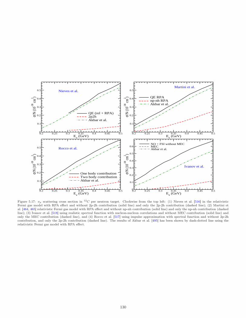
0.2 0.25 0.3 0.35 0.4 0.45 0.5Eν (GeV)

0

0.1

0.2

0.3

0.4

0.5

σ/N

(10-3

8 cm

2 )

QE (rel + RPA)2p2hAkbar et al.

Nieves et al.

0.2 0.25 0.3 0.35 0.4 0.45 0.5Eν (GeV)

0

0.1

0.2

0.3

0.4

0.5

σ/N

(10-3

8 cm

2 ) QE RPAnp-nh RPAAkbar et al.

Martini et al.

0.2 0.25 0.3 0.35 0.4 0.45 0.5Eν (GeV)

0

0.1

0.2

0.3

0.4

0.5

σ/N

(10-3

8 cm

2 )

One body contributionTwo body contributionAkbar et al.

Rocco et al.

0.2 0.25 0.3 0.35 0.4 0.45 0.5Eν (GeV)

0

0.1

0.2

0.3

0.4

0.5

0.6

σ/N

(10-3

8 cm

2 )

NO + FSI without MECMECAkbar et al.

Ivanov et al.

Figure 5.17: νµ scattering cross section in 12C per neutron target. Clockwise from the top left: (1) Nieves et al. [516] in the relativisticFermi gas model with RPA effect and without 2p-2h contribution (solid line) and only the 2p-2h contribution (dashed line); (2) Martini etal. [464, 465] relativistic Fermi gas model with RPA effect and without np-nh contribution (solid line) and only the np-nh contribution (dashedline); (3) Ivanov et al. [518] using realistic spectral function with nucleon-nucleon correlations and without MEC contribution (solid line) andonly the MEC contribution (dashed line), and (4) Rocco et al. [517] using impulse approximation with spectral function and without 2p-2hcontribution, and only the 2p-2h contribution (dashed line). The results of Akbar et al. [495] has been shown by dash-dotted line using therelativistic Fermi gas model with RPA effect.

130

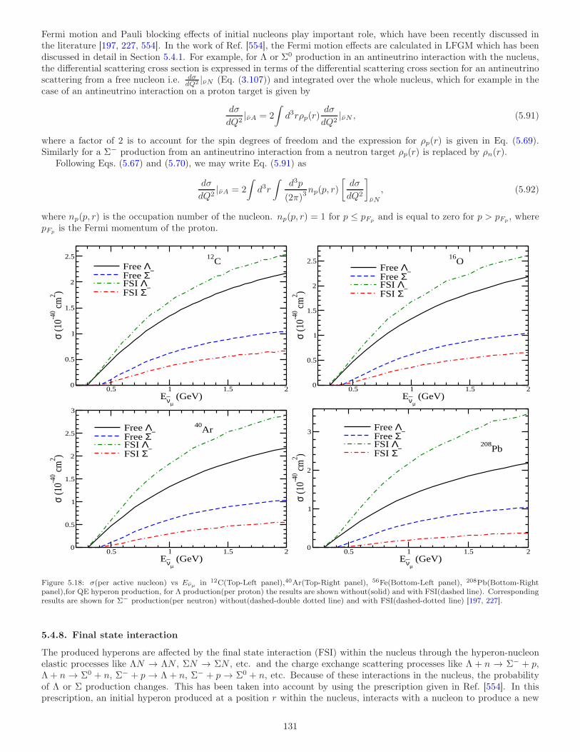
Fermi motion and Pauli blocking effects of initial nucleons play important role, which have been recently discussed inthe literature [197, 227, 554]. In the work of Ref. [554], the Fermi motion effects are calculated in LFGM which has beendiscussed in detail in Section 5.4.1. For example, for Λ or Σ0 production in an antineutrino interaction with the nucleus,the differential scattering cross section is expressed in terms of the differential scattering cross section for an antineutrinoscattering from a free nucleon i.e. dσ

dQ2 |νN (Eq. (3.107)) and integrated over the whole nucleus, which for example in thecase of an antineutrino interaction on a proton target is given by

dσ

dQ2|νA = 2

∫

d3rρp(r)dσ

dQ2|νN , (5.91)

where a factor of 2 is to account for the spin degrees of freedom and the expression for ρp(r) is given in Eq. (5.69).Similarly for a Σ− production from an antineutrino interaction from a neutron target ρp(r) is replaced by ρn(r).

Following Eqs. (5.67) and (5.70), we may write Eq. (5.91) as

dσ

dQ2|νA = 2

∫

d3r

∫

d3p

(2π)3np(p, r)

[

dσ

dQ2

]

νN

, (5.92)

where np(p, r) is the occupation number of the nucleon. np(p, r) = 1 for p ≤ pFpand is equal to zero for p > pFp

, wherepFp

is the Fermi momentum of the proton.

0.5 1 1.5 2Eνµ

(GeV)0

0.5

1

1.5

2

2.5

σ (1

0-40 c

m2 )

Free ΛFree Σ−

FSI ΛFSI Σ−

12C

0.5 1 1.5 2Eνµ

(GeV)0

0.5

1

1.5

2

2.5

σ (1

0-40 c

m2 )

Free ΛFree Σ−

FSI ΛFSI Σ−

16O

0.5 1 1.5 2Eνµ

(GeV)0

0.5

1

1.5

2

2.5

3

σ (1

0-40 c

m2 )

Free ΛFree Σ−

FSI ΛFSI Σ−

40Ar

0.5 1 1.5 2Eνµ

(GeV)0

1

2

3

σ (1

0-40 c

m2 )

Free ΛFree Σ−

FSI ΛFSI Σ−

208Pb

Figure 5.18: σ(per active nucleon) vs Eνµ in 12C(Top-Left panel),40Ar(Top-Right panel), 56Fe(Bottom-Left panel), 208Pb(Bottom-Rightpanel),for QE hyperon production, for Λ production(per proton) the results are shown without(solid) and with FSI(dashed line). Correspondingresults are shown for Σ− production(per neutron) without(dashed-double dotted line) and with FSI(dashed-dotted line) [197, 227].

5.4.8. Final state interaction

The produced hyperons are affected by the final state interaction (FSI) within the nucleus through the hyperon-nucleonelastic processes like ΛN → ΛN , ΣN → ΣN , etc. and the charge exchange scattering processes like Λ + n → Σ− + p,Λ + n → Σ0 + n, Σ− + p → Λ + n, Σ− + p → Σ0 + n, etc. Because of these interactions in the nucleus, the probabilityof Λ or Σ production changes. This has been taken into account by using the prescription given in Ref. [554]. In thisprescription, an initial hyperon produced at a position r within the nucleus, interacts with a nucleon to produce a new

131

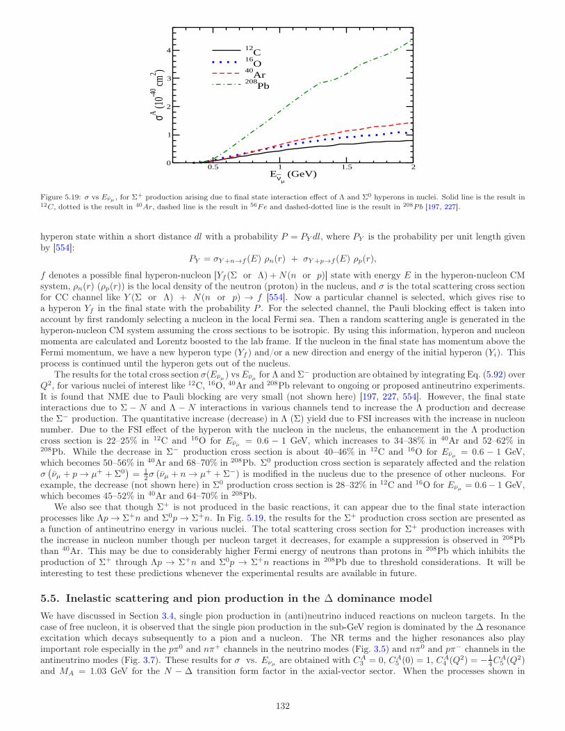
0.5 1 1.5 2Eνµ

(GeV)0

1

2

3

4

σA (10-4

0 cm2 )

12C

16O

40Ar

208Pb

Figure 5.19: σ vs Eνµ , for Σ+ production arising due to final state interaction effect of Λ and Σ0 hyperons in nuclei. Solid line is the result in12C, dotted is the result in 40Ar, dashed line is the result in 56Fe and dashed-dotted line is the result in 208Pb [197, 227].

hyperon state within a short distance dl with a probability P = PY dl, where PY is the probability per unit length givenby [554]:

PY = σY+n→f (E) ρn(r) + σY +p→f (E) ρp(r),

f denotes a possible final hyperon-nucleon [Yf (Σ or Λ) +N(n or p)] state with energy E in the hyperon-nucleon CMsystem, ρn(r) (ρp(r)) is the local density of the neutron (proton) in the nucleus, and σ is the total scattering cross sectionfor CC channel like Y (Σ or Λ) + N(n or p) → f [554]. Now a particular channel is selected, which gives rise toa hyperon Yf in the final state with the probability P . For the selected channel, the Pauli blocking effect is taken intoaccount by first randomly selecting a nucleon in the local Fermi sea. Then a random scattering angle is generated in thehyperon-nucleon CM system assuming the cross sections to be isotropic. By using this information, hyperon and nucleonmomenta are calculated and Lorentz boosted to the lab frame. If the nucleon in the final state has momentum above theFermi momentum, we have a new hyperon type (Yf ) and/or a new direction and energy of the initial hyperon (Yi). Thisprocess is continued until the hyperon gets out of the nucleus.

The results for the total cross section σ(Eνµ ) vsEνµ for Λ and Σ− production are obtained by integrating Eq. (5.92) overQ2, for various nuclei of interest like 12C, 16O, 40Ar and 208Pb relevant to ongoing or proposed antineutrino experiments.It is found that NME due to Pauli blocking are very small (not shown here) [197, 227, 554]. However, the final stateinteractions due to Σ − N and Λ − N interactions in various channels tend to increase the Λ production and decreasethe Σ− production. The quantitative increase (decrease) in Λ (Σ) yield due to FSI increases with the increase in nucleonnumber. Due to the FSI effect of the hyperon with the nucleon in the nucleus, the enhancement in the Λ productioncross section is 22–25% in 12C and 16O for Eνµ = 0.6 − 1 GeV, which increases to 34–38% in 40Ar and 52–62% in208Pb. While the decrease in Σ− production cross section is about 40–46% in 12C and 16O for Eνµ = 0.6 − 1 GeV,which becomes 50–56% in 40Ar and 68–70% in 208Pb. Σ0 production cross section is separately affected and the relationσ(

νµ + p→ µ+ +Σ0)

= 12σ (νµ + n→ µ+ +Σ−) is modified in the nucleus due to the presence of other nucleons. For

example, the decrease (not shown here) in Σ0 production cross section is 28–32% in 12C and 16O for Eνµ = 0.6− 1 GeV,which becomes 45–52% in 40Ar and 64–70% in 208Pb.

We also see that though Σ+ is not produced in the basic reactions, it can appear due to the final state interactionprocesses like Λp→ Σ+n and Σ0p→ Σ+n. In Fig. 5.19, the results for the Σ+ production cross section are presented asa function of antineutrino energy in various nuclei. The total scattering cross section for Σ+ production increases withthe increase in nucleon number though per nucleon target it decreases, for example a suppression is observed in 208Pbthan 40Ar. This may be due to considerably higher Fermi energy of neutrons than protons in 208Pb which inhibits theproduction of Σ+ through Λp → Σ+n and Σ0p → Σ+n reactions in 208Pb due to threshold considerations. It will beinteresting to test these predictions whenever the experimental results are available in future.

5.5. Inelastic scattering and pion production in the ∆ dominance model

We have discussed in Section 3.4, single pion production in (anti)neutrino induced reactions on nucleon targets. In thecase of free nucleon, it is observed that the single pion production in the sub-GeV region is dominated by the ∆ resonanceexcitation which decays subsequently to a pion and a nucleon. The NR terms and the higher resonances also playimportant role especially in the pπ0 and nπ+ channels in the neutrino modes (Fig. 3.5) and nπ0 and pπ− channels in theantineutrino modes (Fig. 3.7). These results for σ vs. Eνµ are obtained with CA

3 = 0, CA5 (0) = 1, CA

4 (Q2) = − 14C

A5 (Q2)

and MA = 1.03 GeV for the N − ∆ transition form factor in the axial-vector sector. When the processes shown in

132

Eqs. (3.82) and (3.95) take place inside the nucleus, there are two possibilities of the pion production i.e. the targetnucleus remains in the ground state leading to coherent production of pions or is excited and/or broken up leading toincoherent production of pions. As these processes take place inside the nucleus, NME come into play, which modifiesthe resonance properties like its mass and width. In literature, the nuclear medium modifications have been studied inthe weak sector only in the case of ∆ excitation, therefore, for the pion production in (anti)neutrino scattering from thenucleus, the calculations have been done in the ∆ dominance model. Both the production processes in the ∆ dominancemodel using the local density approximation have been considered to calculate single pion production from several nucleartargets like 12C, 16O, 40Ar and 208Pb. In the delta dominance model, if one take CA

5 (0) = 1.2 and MA = 1.05 GeV, thenthe results obtained with these parameters for the single pion production from free nucleons almost resemble the pionproduction from the free nucleons when the contribution from the higher resonances and NRB as well as their interferencesare taken with CA

5 (0) = 1 and MA = 1.03 GeV (Fig. 3.5). In this section, we are discussing incoherent pion production.The effect of nuclear medium on the production of ∆ is treated by including the modification of ∆ properties in themedium. Once the pions are produced, they undergo final state interactions with the residual nucleus, which has beentaken into account.

In the local density approximation (Section 5.4.1), the cross section for the reaction say νl(k) + N(p) → l−(k′) +N ′(p′) + πi(pπ), where i = ±, 0 and N,N ′ = p or n inside a nuclear target is evaluated as a function of local Fermimomentum(pF (r)) and integrated over the size of whole nucleus i.e.

(

dσ

dEπdΩπ

)

νA

=

∫

d~r ρN (r)

(

dσ

dEπdΩπ

)

νN

,

where the expression for(

dσdEπdΩπ

)

νNis given in Eq. (3.4) for the free nucleon target. While for the scattering of

(anti)neutrino with a nucleon inside the nucleus, the interacting nucleon is not as rest i.e. EN =√

|~pN |2 +M2 and

E′N =

√

|~p ′N |2 +M2 =

√

|~q − ~pπ + ~pN |2 +M2, and therefore

(

dσ

dEπdΩπ

)

νN

=1

32 (2π)5

∫

dΩ′dE′δ0 (EN (~p) + qo − EN ′(~p′)− Eπ(~pπ))|~k′||~pπ|EENEN ′

(

G2F

2cos2θcLµνJ

µν

)

, (5.93)

where Lµν is the leptonic tensor, the expression for which is given in Eq. (2.15) and the hadronic tensor Jµν = 12

∑

jµjν†

where the hadronic current

jµ = I u(~p ′)fπN∆

mπpσπPσλOλµu(~p), (5.94)

where I =√3 for ∆++ and ∆− excitations, otherwise I = 1. In the above expression Oλµ is the N − ∆ transition

operator, the expression for which is given in Eq. (3.49) and Pσλ is the ∆ propagator in the momentum space, theexpression for which is given in Eq. (3.67).

Following Eqs. (5.67) and (5.70), we may write Eq. (5.93) as(

dσ

dEπdΩπ

)

νA

= 2

∫

d~r∑

N=n,p

d~pN(2π)3

Θ1(ENF (r)− EN )Θ2(EN + q0 − Eπ − EN ′

F (r)) ×(

dσ

dEπdΩπ

)

νN

.

Thus, in the local density approximation the expression for the total cross section for the neutrino induced CC 1π+

production from the nucleon target is written as

σA(E) =1

(4π)5

∫ rmax

rmin

(

ρp(r) +1

9ρn(r)

)

d~r

∫ Q2max

Q2min

dQ2 ×∫ k′

max

k′min

dk′∫ +1

−1

dcosθπ

×∫ 2π

0

dφππ|~k′||~kπ|ME2

νEl

1

E′p + Eπ

(

1− |~q||~kπ|

cosθπ

)

(

G2F

4cos2θcLµνJ

µν

)

(5.95)

For 1π− production(

ρp(r) +19ρn(r)

)

in the above expression, is replaced by(

ρn(r) +19ρp(r)

)

and for the π0 production,it is replaced by 2

3 (ρp(r) + ρn(r)), where ρp(r) and ρn(r) are already defined in Section 5.4.1.The nuclear medium modification on the ∆ properties like the modification in its mass and width arises from the

following sources:

(a) The intermediate nucleon state is partly blocked for the ∆ decay because some of these states are occupied (Pauliblocking). The decayed nucleon must be in an unoccupied state. The Pauli correction is taken into account byassuming a local Fermi sea at each point of the nucleus of density ρ(r), and forcing the nucleon to be above theFermi sea. This leads to an energy dependent modification in the ∆ decay width given as [555]:

Γ→ Γ− 2ImΣ∆, (5.96)

133

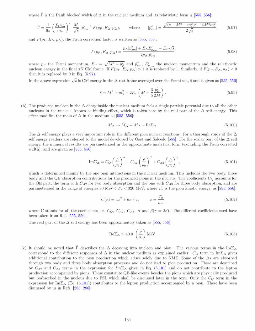
where Γ is the Pauli blocked width of ∆ in the nuclear medium and its relativistic form is [555, 556]:

Γ =1

6π

(

fπN∆

mπ

)2M√s|~p ′

cm|3 F (pF , E∆, p∆), where |~p ′cm| =

√

(s−M2 −m2π)

2 − 4M2m2π

2√s

, (5.97)

and F (pF , E∆, p∆), the Pauli correction factor is written as [555, 556]:

F (pF , E∆, p∆) =p∆|~p ′

cm|+ E∆E′pcm− EF

√s

2p∆|~p ′cm|

(5.98)

where pF the Fermi momentum, EF =√

M2 + p2F and ~p ′cm, E′

pcmthe nucleon momentum and the relativistic

nucleon energy in the final πN CM frame. If F (pF , E∆, p∆) > 1 it is replaced by 1. Similarly, if F (pF , E∆, p∆) < 0then it is replaced by 0 in Eq. (5.97).

In the above expression√s is CM energy in the ∆ rest frame averaged over the Fermi sea, s and is given as [555, 556]

s =M2 +m2π + 2Eπ

(

M +3

5

p2F2M

)

. (5.99)

(b) The produced nucleon in the ∆ decay inside the nuclear medium feels a single particle potential due to all the othernucleons in the nucleus, known as binding effect, which is taken care by the real part of the ∆ self energy. Thiseffect modifies the mass of ∆ in the medium as [555, 556]:

M∆ → M∆ =M∆ + ReΣ∆. (5.100)

The ∆ self energy plays a very important role in the different pion nuclear reactions. For a thorough study of the ∆self energy readers are referred to the model developed by Oset and Salcedo [555]. For the scalar part of the ∆ selfenergy, the numerical results are parameterized in the approximate analytical form (excluding the Pauli correctedwidth), and are given as [555, 556]:

−ImΣ∆ = CQ

(

ρ

ρ0

)α

+ CA2

(

ρ

ρ0

)β

+ CA3

(

ρ

ρ0

)γ

, (5.101)

which is determined mainly by the one pion interactions in the nuclear medium. This includes the two body, threebody and the QE absorption contributions for the produced pions in the nucleus. The coefficients CQ accounts forthe QE part, the term with CA2 for two body absorption and the one with CA3 for three body absorption, and areparameterized in the range of energies 80 MeV< Tπ < 320 MeV, where Tπ is the pion kinetic energy, as [555, 556]:

C(x) = ax2 + bx+ c, x =Tπmπ

(5.102)

where C stands for all the coefficients i.e. CQ, CA2, CA3, α and β(γ = 2β). The different coefficients used havebeen taken from Ref. [555, 556].

The real part of the ∆ self energy has been approximately taken as [555, 556]

ReΣ∆ ≃ 40.0

(

ρ

ρ0

)

MeV. (5.103)

(c) It should be noted that Γ describes the ∆ decaying into nucleon and pion. The various terms in the ImΣ∆

correspond to the different responses of ∆ in the nuclear medium as explained earlier. CQ term in ImΣ∆ givesadditional contribution to the pion production which arises solely due to NME. Some of the ∆s are absorbedthrough two body and three body absorption processes and do not lead to pion production. These are describedby CA2 and CA3 terms in the expression for ImΣ∆ given in Eq. (5.101) and do not contribute to the leptonproduction accompanied by pions. These constitute QE-like events besides the pions which are physically producedbut reabsorbed in the nucleus due to FSI, which shall be discussed later in the text. Only the CQ term in theexpression for ImΣ∆ (Eq. (5.101)) contributes to the lepton production accompanied by a pion. These have beendiscussed by us in Refs. [285, 286].

134

N R

N

πiW+(Z0)

νl

l−(νl)

πl

Pionproduction

πj πk N R

N

πiW+(Z0)

νl

l−(νl)

Pionabsorption

πj

Figure 5.20: Pion production inside a nuclear target and its interaction with the nucleons in the nucleus while coming out. The pions mayundergo elastic scattering, charge exchange (for example π+ + n → π0 + p) reaction, etc. and therefore the charge of pion may change onway before it comes out of the nucleus (left panel). In a neutrino induced reaction on a nucleon target when a pion is absorbed in the nuclearmedium while coming out (right panel). The open (shaded) circles represent protons (neutrons) inside a nucleus and the dark shaded circlerepresents a nucleon (p or n) with which a neutrino interacts through a CC (NC) reaction and a NR or a resonance state (R) is formed, whichgives rise to a proton or a neutron and a pion (πi), where i represents the charge state.

5.5.1. Final state interaction effect

The pions which are produced in these processes while traveling inside the nucleus can be absorbed, can change direction,energy, charge, or even produce more pions due to various processes like elastic and charge exchange scattering with thenucleons present in the nucleus through strong interactions. Therefore, the production cross sections for the pions from thenuclear targets are affected by the presence of strong interactions of final state pions in the nuclear medium (Fig. 5.20).For example, a pion produced in the nuclear medium may get absorbed by the nucleons and thus mimicking a QE-like event (see Fig. 5.20) or can suffer elastic, and charge exchange scattering with the nucleons. There are generallytwo approaches to treat these final state interactions of pions. In one approach, the distortion of pion wave functionsis calculated in an optical potential by solving the Schrodinger or Klein-Gordon equation of motion or approximationmethods using Glauber model is used. In another approach, a microscopic method is used in which the motion of the pioninside the nucleus is followed step by step in which the pion suffers interaction with the nucleon. This approach is discussedby Vicente Vacas et al. [557] and is used by us in many calculations of treating the FSI of pions [284, 286, 558, 559].

This final state interaction of pions is treated using Monte Carlo simulations by generating pion of given momentumand charge at point ~r in the nucleus. Assuming the real part of the pion nuclear potential to be weak as compared totheir kinetic energies they are propagated in straight lines till they are out of the nucleus. At the beginning they areplaced at (~b, zin), with a random impact parameter ~b, with |~b| < R, where R is the nuclear radius which is taken to be

a point where nuclear density ρ(R) falls to 10−3ρ0, where ρ0 is the central density, and zin = −√

R2 − |~b|2. Then it is

moved in small steps δl along the z-direction until it comes out of the nucleus or interact. If P (pπ, r, λ) is the probabilityper unit length at the point r of a pion of momentum ~pπ and charge λ, then Pδl << 1. A random number x is generatedsuch that x ∈ [0, 1] and if x > Pδl, then it is assumed that pion has not interacted while traveling a distance δl, however,if x < Pδl then the pion has interacted and depending upon the weight factor of each channel given by its cross sectionit is decided that whether the interaction was QE, charge exchange reaction, pion production or pion absorption [557].For example, for the QE scattering

PN(πλ,πλ′)N ′ = σN(πλ,πλ′)N ′ × ρN

where N is a nucleon, ρN is its density and σ is the elementary cross section for the reaction πλ +N → πλ′

+N ′ obtainedfrom the phase shift analysis. For a pion to be absorbed, P is expressed in terms of the imaginary part of the pion self

energy Π i.e. Pabs = − ImΠabs(pπ)pπ

, where the self energy Π is related to the pion optical potential V (~r) [557].

In Fig. 5.21, results for the Q2 distribution dσdQ2 and the pion momentum distribution dσ

dpπare shown for CC νµ(νµ)

induced incoherent one π+ (π−) production cross section. These results are presented for the differential scattering crosssection calculated with and without NME and with NME including the pion absorption effects. For the Q2-distributionshown in Fig. 5.21, it may be seen that the reduction in the cross section as compared to the cross section calculatedwithout NME is around 35% in the peak region. When pion absorption effects are also taken into account there is a furtherreduction of around 15%. The results for the antineutrino induced one π− production cross section are qualitatively similarin nature but quantitatively we find that the peak shifts towards a slightly lower value of Q2. In Fig. 5.21, the resultsfor the pion momentum distribution have been shown. In this case, the reduction in the cross section in the peak regionis around 40% when NME are taken into account, which further reduces by about 15% when pion absorption effects arealso taken into account.

In Fig. 5.22, the results for the total scattering cross section σ for CC νµ (νµ) induced one π+ (π−) production crosssection are shown. With the inclusion of NME the reduction in the cross section from the cross section calculated without

135

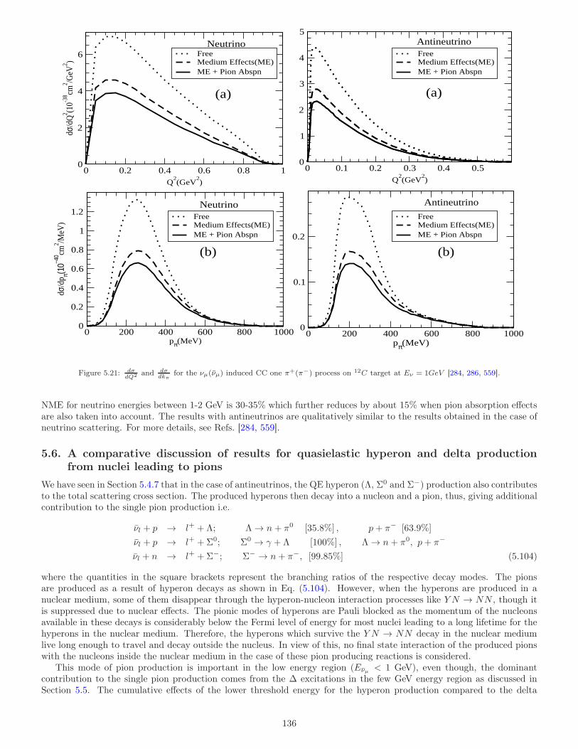
0 0.2 0.4 0.6 0.8 1Q

2(GeV

2)

0

2

4

6

dσ/d

Q2 (1

0-38 cm

2 /GeV

2 )

FreeMedium Effects(ME)ME + Pion Abspn

0 0.1 0.2 0.3 0.4 0.5Q

2(GeV

2)

0

1

2

3

4

5

FreeMedium Effects(ME)ME + Pion Abspn

0 200 400 600 800 1000pπ(MeV)

0

0.2

0.4

0.6

0.8

1

1.2

dσ/d

p π(10−4

0 cm2 /M

eV)

FreeMedium Effects(ME)ME + Pion Abspn

0 200 400 600 800 1000pπ(MeV)

0

0.1

0.2

FreeMedium Effects(ME)ME + Pion Abspn

Neutrino

Neutrino Antineutrino

Antineutrino

(a) (a)

(b) (b)

Figure 5.21: dσdQ2 and dσ

dkπfor the νµ(νµ) induced CC one π+(π−) process on 12C target at Eν = 1GeV [284, 286, 559].

NME for neutrino energies between 1-2 GeV is 30-35% which further reduces by about 15% when pion absorption effectsare also taken into account. The results with antineutrinos are qualitatively similar to the results obtained in the case ofneutrino scattering. For more details, see Refs. [284, 559].

5.6. A comparative discussion of results for quasielastic hyperon and delta productionfrom nuclei leading to pions

We have seen in Section 5.4.7 that in the case of antineutrinos, the QE hyperon (Λ, Σ0 and Σ−) production also contributesto the total scattering cross section. The produced hyperons then decay into a nucleon and a pion, thus, giving additionalcontribution to the single pion production i.e.

νl + p → l+ + Λ; Λ→ n+ π0 [35.8%] , p+ π− [63.9%]

νl + p → l+ +Σ0; Σ0 → γ + Λ [100%] , Λ→ n+ π0, p+ π−

νl + n → l+ +Σ−; Σ− → n+ π−, [99.85%] (5.104)

where the quantities in the square brackets represent the branching ratios of the respective decay modes. The pionsare produced as a result of hyperon decays as shown in Eq. (5.104). However, when the hyperons are produced in anuclear medium, some of them disappear through the hyperon-nucleon interaction processes like Y N → NN , though itis suppressed due to nuclear effects. The pionic modes of hyperons are Pauli blocked as the momentum of the nucleonsavailable in these decays is considerably below the Fermi level of energy for most nuclei leading to a long lifetime for thehyperons in the nuclear medium. Therefore, the hyperons which survive the Y N → NN decay in the nuclear mediumlive long enough to travel and decay outside the nucleus. In view of this, no final state interaction of the produced pionswith the nucleons inside the nuclear medium in the case of these pion producing reactions is considered.

This mode of pion production is important in the low energy region (Eνµ < 1 GeV), even though, the dominantcontribution to the single pion production comes from the ∆ excitations in the few GeV energy region as discussed inSection 5.5. The cumulative effects of the lower threshold energy for the hyperon production compared to the delta

136

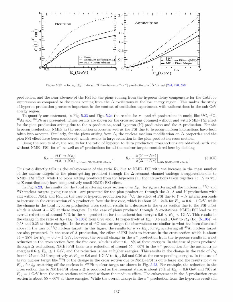
0.5 1 1.5 2Eν(GeV)

0

1

2

3

4

5

6

σ (1

0-38 cm

2 )

FreeMedium Effects(ME)ME + Pion Abspn

0.5 1 1.5 2Eν(GeV)

0

0.4

0.8

1.2

1.6

2

2.4

FreeMedium Effects(ME)ME + Pion Abspn

Neutrino Antineutrino

Figure 5.22: σ for νµ (νµ) induced CC incoherent π+(π−) production on 12C target [284, 286, 559].

production, and the near absence of the FSI for the pions coming from the hyperon decay compensate for the Cabibbosuppression as compared to the pions coming from the ∆ excitations in the low energy region. This makes the studyof hyperon production processes important in the context of oscillation experiments with antineutrinos in the sub-GeVenergy region.

To quantify our statement, in Fig. 5.23 and Figs. 5.24 the results for π− and π0 productions in nuclei like 12C, 16O,40Ar and 208Pb are presented. These results are shown for the cross sections obtained without and with NME+FSI effectfor the pion production arising due to the Λ production, total hyperon (Y ) production and the ∆ production. For thehyperon production, NMEs in the production process as well as the FSI due to hyperon-nucleon interactions have beentaken into account. Similarly, for the pions arising from ∆, the nuclear medium modification on ∆ properties and thepion FSI effect have been considered, which results in large reduction in the pion production cross section.

Using the results of σ, the results for the ratio of hyperon to delta production cross sections are obtained, with andwithout NME+FSI, for π− as well as π0 productions for all the nuclear targets considered here by defining

RN =σ(Y → Nπ)

σ(∆→ Nπ)

∣

∣

∣

∣

without NME+FSI effects

, RA =σ(Y → Nπ)

σ(∆→ Nπ)

∣

∣

∣

∣

with NME+FSI effects

. (5.105)

This ratio directly tells us the enhancement of the ratio RA due to NME+FSI with the increase in the mass numberof the nuclear targets as the pions getting produced through the ∆-resonant channel undergo a suppression due toNME+FSI effect, while the pions getting produced from the hyperons (all the interactions taken together i.e. Λ as wellas Σ contributions) have comparatively small NME+FSI effect.

In Fig. 5.23, the results for the total scattering cross section σ vs Eνµ , for νµ scattering off the nucleon in 12C and16O nuclear targets giving rise to π− are presented for the pion production through the ∆, Λ and Y productions withand without NME and FSI. In the case of hyperon production for 12C, the effect of FSI due to Y −N interaction leadsto increase in the cross section of Λ production from the free case, which is about 23− 24% for Eνµ = 0.6− 1 GeV, whilethe change in the total hyperon production cross section results in a decrease in the cross section due to the FSI effectwhich is about 3 − 5% at these energies. In the case of pions produced through ∆ excitations, NME+FSI lead to anoverall reduction of around 50% in the π− production for the antineutrino energies 0.6 < Eνµ < 1GeV. This results inthe change in the ratio of RN (Eq. (5.105)) from 0.28 and 0.14 respectively at Eνµ=0.6 and 1 GeV to RA (Eq. (5.105)) →0.58 and 0.25 at these energies. In the case of 16O nuclear target the observations are similar to what has been discussedabove in the case of 12C nuclear target. In this figure, the results for σ vs Eνµ , for νµ scattering off 40Ar nuclear targetare also presented. In the case of Λ production, the effect of FSI leads to increase in the cross section which is about34 − 38% for Eνµ = 0.6 − 1 GeV, however, the overall change in the π− production from the hyperons results in a netreduction in the cross section from the free case, which is about 6 − 8% at these energies. In the case of pions producedthrough ∆ excitations, NME+FSI leads to a reduction of around 55 − 60% in the π− production for the antineutrinoenergies 0.6 ≤ Eνµ ≤ 1 GeV, and the reduction is less at higher energies. This results in the change in the ratio of RN

from 0.25 and 0.13 respectively at Eνµ = 0.6 and 1 GeV to RA, 0.6 and 0.26 at the corresponding energies. In the case ofheavy nuclear target like 208Pb, the change in the cross section due to NME+FSI is quite large and the results for σ vsEνµ , for νµ scattering off the nucleon in 208Pb nuclear target are shown in Fig. 5.23. For example, the reduction in thecross section due to NME+FSI when a ∆ is produced as the resonant state, is about 75% at Eνµ = 0.6 GeV and 70% atEνµ = 1 GeV from the cross sections calculated without the medium effect. The enhancement in the Λ production crosssection is about 55− 60% at these energies. While the overall change in the π− production from the hyperons results in

137

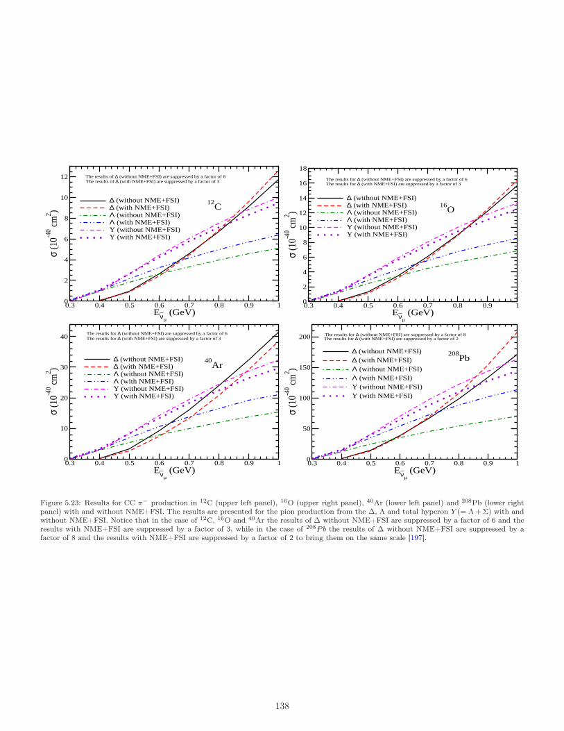
0.3 0.4 0.5 0.6 0.7 0.8 0.9 1Eνµ

(GeV)0

2

4

6

8

10

12

σ (1

0-40 c

m2 )

∆ (without NME+FSI)∆ (with NME+FSI)Λ (without NME+FSI)Λ (with NME+FSI)Y (without NME+FSI)Y (with NME+FSI)

The results of ∆ (without NME+FSI) are suppressed by a factor of 6

12C

The results of ∆ (with NME+FSI) are suppressed by a factor of 3

0.3 0.4 0.5 0.6 0.7 0.8 0.9 1Eνµ

(GeV)0

2

4

6

8

10

12

14

16

18

σ (1

0-40 c

m2 )

∆ (without NME+FSI)∆ (with NME+FSI)Λ (without NME+FSI)Λ (with NME+FSI)Y (without NME+FSI)Y (with NME+FSI)

16O

The results for ∆ (without NME+FSI) are suppressed by a factor of 6The results for ∆ (with NME+FSI) are suppressed by a factor of 3

0.3 0.4 0.5 0.6 0.7 0.8 0.9 1Eνµ

(GeV)0

10

20

30

40

σ (1

0-40 c

m2 )

∆ (without NME+FSI)∆ (with NME+FSI)Λ (without NME+FSI)Λ (with NME+FSI)Y (without NME+FSI)Y (with NME+FSI)

The results for ∆ (without NME+FSI) are suppressed by a factor of 6

40Ar

The results for ∆ (with NME+FSI) are suppressed by a factor of 3

0.3 0.4 0.5 0.6 0.7 0.8 0.9 1Eνµ

(GeV)0

50

100

150

200

σ (1

0-40 c

m2 )

∆ (without NME+FSI)∆ (with NME+FSI)Λ (without NME+FSI)Λ (with NME+FSI)Y (without NME+FSI)Y (with NME+FSI)

The results for ∆ (without NME+FSI) are suppressed by a factor of 8

208Pb

The results for ∆ (with NME+FSI) are suppressed by a factor of 2

Figure 5.23: Results for CC π− production in 12C (upper left panel), 16O (upper right panel), 40Ar (lower left panel) and 208Pb (lower rightpanel) with and without NME+FSI. The results are presented for the pion production from the ∆, Λ and total hyperon Y (= Λ+Σ) with andwithout NME+FSI. Notice that in the case of 12C, 16O and 40Ar the results of ∆ without NME+FSI are suppressed by a factor of 6 and theresults with NME+FSI are suppressed by a factor of 3, while in the case of 208Pb the results of ∆ without NME+FSI are suppressed by afactor of 8 and the results with NME+FSI are suppressed by a factor of 2 to bring them on the same scale [197].

138

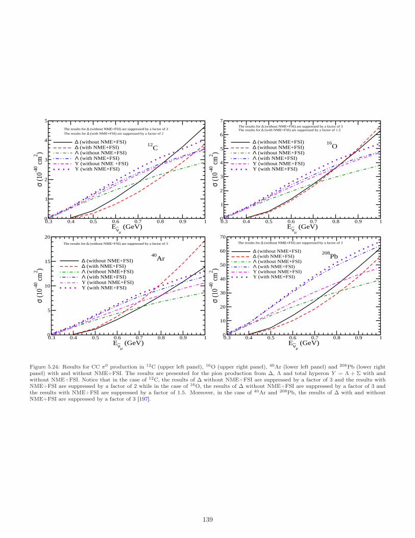
0.3 0.4 0.5 0.6 0.7 0.8 0.9 1Eνµ

(GeV)0

1

2

3

4

5

σ (1

0-40 c

m2 )

∆ (without NME+FSI)∆ (with NME+FSI)Λ (without NME+FSI)Λ (with NME+FSI)Y (without NME +FSI)Y (with NME+FSI)

The results for ∆ (with NME+FSI) are suppressed by a factor of 2

12C

The results for ∆ (without NME+FSI) are suppressed by a factor of 3

0.3 0.4 0.5 0.6 0.7 0.8 0.9 1Eνµ

(GeV)0

1

2

3

4

5

6

7

σ (1

0-40 c

m2 )

∆ (without NME+FSI)∆ (without NME+FSI)Λ (without NME+FSI)Λ (with NME+FSI)Y (without NME+FSI)Y (with NME+FSI)

The results for ∆ (without NME+FSI) are suppressed by a factor of 3

16O

The results for ∆ (with NME+FSI) are suppressed by a factor of 1.5

0.3 0.4 0.5 0.6 0.7 0.8 0.9 1Eνµ

(GeV)0

5

10

15

20

σ (1

0-40 c

m2 )

∆ (without NME+FSI)∆ (with NME+FSI)Λ (without NME+FSI)Λ (with NME+FSI)Y (without NME+FSI)Y (with NME+FSI)

40Ar

The results for ∆ (without NME+FSI) are suppressed by a factor of 3

0.3 0.4 0.5 0.6 0.7 0.8 0.9 1Eνµ

(GeV)0

10

20

30

40

50

60

70

σ (1

0-40 c

m2 )

∆ (without NME+FSI)∆ (with NME+FSI)Λ (without NME+FSI)Λ (with NME+FSI)Y (without NME+FSI)Y (with NME+FSI)

The results for ∆ (without NME+FSI) are suppressed by a factor of 3

208Pb

Figure 5.24: Results for CC π0 production in 12C (upper left panel), 16O (upper right panel), 40Ar (lower left panel) and 208Pb (lower rightpanel) with and without NME+FSI. The results are presented for the pion production from ∆, Λ and total hyperon Y = Λ + Σ with andwithout NME+FSI. Notice that in the case of 12C, the results of ∆ without NME+FSI are suppressed by a factor of 3 and the results withNME+FSI are suppressed by a factor of 2 while in the case of 16O, the results of ∆ without NME+FSI are suppressed by a factor of 3 andthe results with NME+FSI are suppressed by a factor of 1.5. Moreover, in the case of 40Ar and 208Pb, the results of ∆ with and withoutNME+FSI are suppressed by a factor of 3 [197].

139

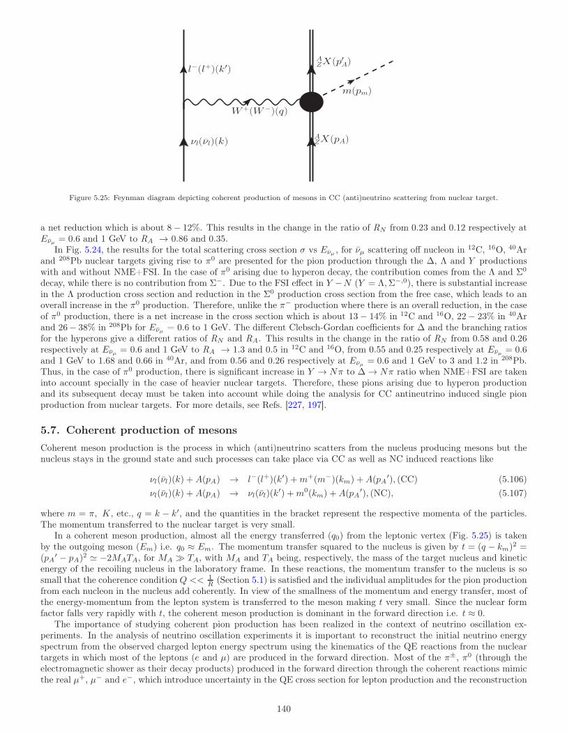
W+(W−)(q)

m(pm)

νl(νl)(k)

l−(l+)(k′)AZX(p′A)

AZX(pA)

Figure 5.25: Feynman diagram depicting coherent production of mesons in CC (anti)neutrino scattering from nuclear target.

a net reduction which is about 8− 12%. This results in the change in the ratio of RN from 0.23 and 0.12 respectively atEνµ = 0.6 and 1 GeV to RA → 0.86 and 0.35.

In Fig. 5.24, the results for the total scattering cross section σ vs Eνµ , for νµ scattering off nucleon in 12C, 16O, 40Arand 208Pb nuclear targets giving rise to π0 are presented for the pion production through the ∆, Λ and Y productionswith and without NME+FSI. In the case of π0 arising due to hyperon decay, the contribution comes from the Λ and Σ0

decay, while there is no contribution from Σ−. Due to the FSI effect in Y −N (Y = Λ,Σ−,0), there is substantial increasein the Λ production cross section and reduction in the Σ0 production cross section from the free case, which leads to anoverall increase in the π0 production. Therefore, unlike the π− production where there is an overall reduction, in the caseof π0 production, there is a net increase in the cross section which is about 13− 14% in 12C and 16O, 22− 23% in 40Arand 26− 38% in 208Pb for Eνµ = 0.6 to 1 GeV. The different Clebsch-Gordan coefficients for ∆ and the branching ratiosfor the hyperons give a different ratios of RN and RA. This results in the change in the ratio of RN from 0.58 and 0.26respectively at Eνµ = 0.6 and 1 GeV to RA → 1.3 and 0.5 in 12C and 16O, from 0.55 and 0.25 respectively at Eνµ = 0.6and 1 GeV to 1.68 and 0.66 in 40Ar, and from 0.56 and 0.26 respectively at Eνµ = 0.6 and 1 GeV to 3 and 1.2 in 208Pb.Thus, in the case of π0 production, there is significant increase in Y → Nπ to ∆→ Nπ ratio when NME+FSI are takeninto account specially in the case of heavier nuclear targets. Therefore, these pions arising due to hyperon productionand its subsequent decay must be taken into account while doing the analysis for CC antineutrino induced single pionproduction from nuclear targets. For more details, see Refs. [227, 197].

5.7. Coherent production of mesons

Coherent meson production is the process in which (anti)neutrino scatters from the nucleus producing mesons but thenucleus stays in the ground state and such processes can take place via CC as well as NC induced reactions like

νl(νl)(k) +A(pA) → l−(l+)(k′) +m+(m−)(km) +A(pA′), (CC) (5.106)

νl(νl)(k) +A(pA) → νl(νl)(k′) +m0(km) +A(pA

′), (NC), (5.107)

where m = π, K, etc., q = k − k′, and the quantities in the bracket represent the respective momenta of the particles.The momentum transferred to the nuclear target is very small.

In a coherent meson production, almost all the energy transferred (q0) from the leptonic vertex (Fig. 5.25) is takenby the outgoing meson (Em) i.e. q0 ≈ Em. The momentum transfer squared to the nucleus is given by t = (q − km)2 =(pA

′ − pA)2 ≃ −2MATA, for MA ≫ TA, with MA and TA being, respectively, the mass of the target nucleus and kineticenergy of the recoiling nucleus in the laboratory frame. In these reactions, the momentum transfer to the nucleus is sosmall that the coherence condition Q << 1

R (Section 5.1) is satisfied and the individual amplitudes for the pion productionfrom each nucleon in the nucleus add coherently. In view of the smallness of the momentum and energy transfer, most ofthe energy-momentum from the lepton system is transferred to the meson making t very small. Since the nuclear formfactor falls very rapidly with t, the coherent meson production is dominant in the forward direction i.e. t ≈ 0.

The importance of studying coherent pion production has been realized in the context of neutrino oscillation ex-periments. In the analysis of neutrino oscillation experiments it is important to reconstruct the initial neutrino energyspectrum from the observed charged lepton energy spectrum using the kinematics of the QE reactions from the nucleartargets in which most of the leptons (e and µ) are produced in the forward direction. Most of the π±, π0 (through theelectromagnetic shower as their decay products) produced in the forward direction through the coherent reactions mimicthe real µ+, µ− and e−, which introduce uncertainty in the QE cross section for lepton production and the reconstruction

140

of the neutrino energy. For example, around 1GeV this uncertainty could be in the range 150-200 MeV. A knowledgeof these uncertainties is crucial in interpreting the results for νµ(νµ) disappearance or νe(νe) appearance in the contextof neutrino oscillation studies making the study of coherent pion production very important in the neutrino-nucleusreactions.

5.7.1. Coherent pion production

Experimentally the coherent pion production in the high energy region was first reported by the Aachen-Padova col-laboration [560] in 1983 while studying isolated π0s produced in the νµ and νµ induced processes. This was followedby a study performed by the Aachen-Gargamelle group [561] where coherent NC π0 events in the Gargamelle heavyfreon exposure were isolated. Later there were several νµ and νµ experiments like CHARM [562, 563], SKAT [564, 565],where NC induced coherent pions were observed over a wide range of neutrino energies using different nuclear targets.In the recent accelerator experiments being performed to study neutrino oscillations like the K2K [566], SciBooNE [567],MiniBooNE [568], NOvA [569], T2K [570], etc., as well as the dedicated ν −A cross section experiment MINERvA [571]and NOMAD [572] experiments have put either a limit on coherent pion cross section or have provided cross sections atsome energies. For example:

• The K2K experiment [566] at a neutrino energy of 1.3 GeV, has put an upper limit of 0.6×10−2 on the cross sectionratio of coherent pion production to the total CC interaction cross section at 90%CL.

• The SciBooNE experiment [567] at neutrino energy of 1.1 GeV, has put an upper limit of 0.67× 10−2 on the crosssection ratio of coherent pion production to the total CC interaction cross section at 90%CL.

• The MiniBooNE collaboration [568] has studied the coherent fractionσ(coh)

σ(coh+incoh)= 19.5± 1.1(stat)± 2.5(sys)% for

the π0 production at Eν < 2 GeV.

• The NOMAD experiment [572] at the CERN SPS has reported NC induced coherent π0 production cross section

to be 72.6± 8.1(stat)± 6.9(sys)× 10−40 cm2

nucleus for < Eν >≃ 25 GeV.

• The T2K experiment [570] has reported a value of 1.03±0.25(stat)±0.70(sys)×10−39 cm2

nucleus for < Eν >≃ 1.5 GeV.

• MINERvA collaboration [571] has reported the flux-averaged cross sections for the coherent π+(π−) productioninduced by νµ(νµ) on the carbon target to be [3.49± 0.11(stat)± 0.37(flux)± 0.20(other-sys)]([2.65± 0.15(stat)±0.31(flux)± 0.30(other-sys)])× 10−39 cm2

12C , respectively, for Eν in the range of 1.5 to 20 GeV.

• Recently the NOvA collaboration [569] has reported the result of the flux averaged cross section for the neutrinoinduced NC coherent π0 production corresponding to an average energy of < Eνµ >= 2.7 GeV to be 13.8±0.9(stat)±2.3(syst)× 10−40cm2/nucleus.

Theoretically there are two different approaches which have been used to study the coherent pion production. Thefirst approach based on the Adler’s PCAC based model [231] which relates the coherent pion scattering cross section atQ2 = 0 with the pion-nucleus elastic scattering cross section. This approach takes NME into account only through thefinal state interaction of the outgoing pions with the nucleus. The first calculation based on this approach was done byRein and Sehgal [131] followed by many others in later years [573, 574, 575, 576, 577].

In this approach, the triple differential cross section for π0 production is given by [131]:

dσπ0

dx dy d|t| =G2

FMf2πA

2

2π2E(1− y) 1

16π(σπN

tot )2(1 + r2)

(

m2A

m2A +Q2

)2

e−b|t|Fabs, (5.108)

where x = Q2/2Mν, y = ν/E, σπN is the pion-nucleon cross section, fπ is the pion decay constant, mA is 1GeV, Mdenotes the nucleon mass, A is the number of nucleons within the nucleus, r (= RefπN(0)/ImfπN(0)) is defined as theratio of the real to imaginary part of the forward pion-nucleon scattering amplitude, b = 1/3R2, with R(R = R0A

1/3) asthe nuclear radius, and Fabs describes the effects of pion absorption in the nucleus, and is given by

Fabs = exp

− 9A1/3

16πR20

σπNinel

, (5.109)

where the experimental results for the average pion-nucleon cross section were used.The above expression was obtained for the massless leptons even for the CC process. In a later work, Rein and

Sehgal [574] took into account the lepton mass by introducing a multiplicative correction factor.Later, Berger and Sehgal [576] used experimental data for pion-carbon scattering in the low energy region relevant

for the contemporary cross section measurements of the coherent pion production in this energy region to describe the

141

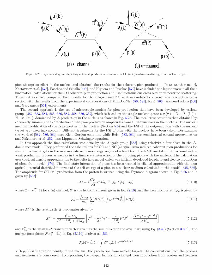
νµ(k)

µ −

W (q)+ νµ(k)

µ −

W (q)+ππ+

+(k ) (k )

(p )π (p )

π

(a) s−channel (b) u−channel

p (p) p (p) p (p)p (p)

∆++(P)

∆o(P)

Figure 5.26: Feynman diagram depicting coherent production of mesons in CC (anti)neutrino scattering from nuclear target.

pion absorption effect in the nucleus and obtained the results for the coherent pion production. In an another model,Kartavtsev et al. [578], Paschos and Schalla [577], and Higuera and Paschos [579] have included the lepton mass in all theirkinematical calculations for the CC coherent pion production and used pion-nucleus cross section in neutrino scattering.These authors have compared their results for the charged and NC neutrino induced coherent pion production crosssection with the results from the experimental collaborations of MiniBooNE [580, 581], K2K [566], Aachen-Padova [560]and Gargamelle [561] experiments.

The second approach is the use of microscopic models for pion production that have been developed by variousgroups [582, 583, 584, 585, 586, 587, 588, 589, 352], which is based on the single nucleon process νl(νl) +N → l−(l+) +N+π+(π−), dominated by ∆ production in the nucleus as shown in Fig. 5.26. The total cross section is then obtained bycoherently summing the contribution of the pion production amplitudes from all the nucleons in the nucleus. The nuclearmedium modification of the ∆ properties in the nucleus (Section 5.5) and the FSI of the outgoing pion with the nucleartarget are taken into account. Different treatments for the FSI of pion with the nucleus have been taken. For examplethe work of [582, 586, 584] uses Klein-Gordon equation, while Refs. [583, 589] use semiclassical eikonal approximationand Nakamura et al [352] uses Lippmann-Schwinger equation.

In this approach the first calculation was done by the Aligarh group [583] using relativistic formalism in the ∆-dominance model. They performed the calculations for CC and NC (anti)neutrino induced coherent pion productions forseveral nuclear targets in the intermediate neutrino energy region of a few GeV. The NME are taken into account in theweak production process as well as in the final state interaction of the outgoing pions with the nucleus. The calculationuses the local density approximation to the delta hole model which was initially developed for photo and electro productionof pions from nuclei [474]. The final state interaction of pions has been treated in eikonal approximation with the pionoptical potential described in terms of the self energy of a pion in a nuclear medium calculated in this model [555, 556].The amplitude for CC 1π+ production from the proton is written using the Feynman diagram shown in Fig. 5.26 and isgiven by [583]:

M = IGF√2

cos θC lµ Jµ Fp(~q − ~kπ) (5.110)

where I =√3 (1) for s (u) channel, lµ is the leptonic current given in Eq. (2.10) and the hadronic current Jµ is given by

Jµ =fπN∆

mπ

∑

s

Ψs(p′)[

kπσΛσλΓ

32νµ

]

Ψs(p) (5.111)

where Λσλ is the relativistic ∆ propagator given by

Λσλ =/P +M∆

P 2 −M2∆ + iΓM∆

[

gσλ − 1

3γσγλ − 2

3M2∆

P σPλ +(P σγλ − γσPλ)

3M∆

]

(5.112)

and Γ32νµ is the weak N-∆ transition vertex given as the sum of vector and axial part using Eq. (3.49) (Section 3.3.5). The

nuclear form factor Fp(~q − ~kπ) in Eq. (5.110) is given as [583]:

Fp(~q − ~kπ) =∫

d~r ρp(r) e−i(~q−~kπ).~r (5.113)

with ρp(r) is the proton density in the nucleus. For production from nuclear targets, the contributions from the protonsand neutrons are considered. Incorporating the isospin factors for charged pion production from proton and neutron

142

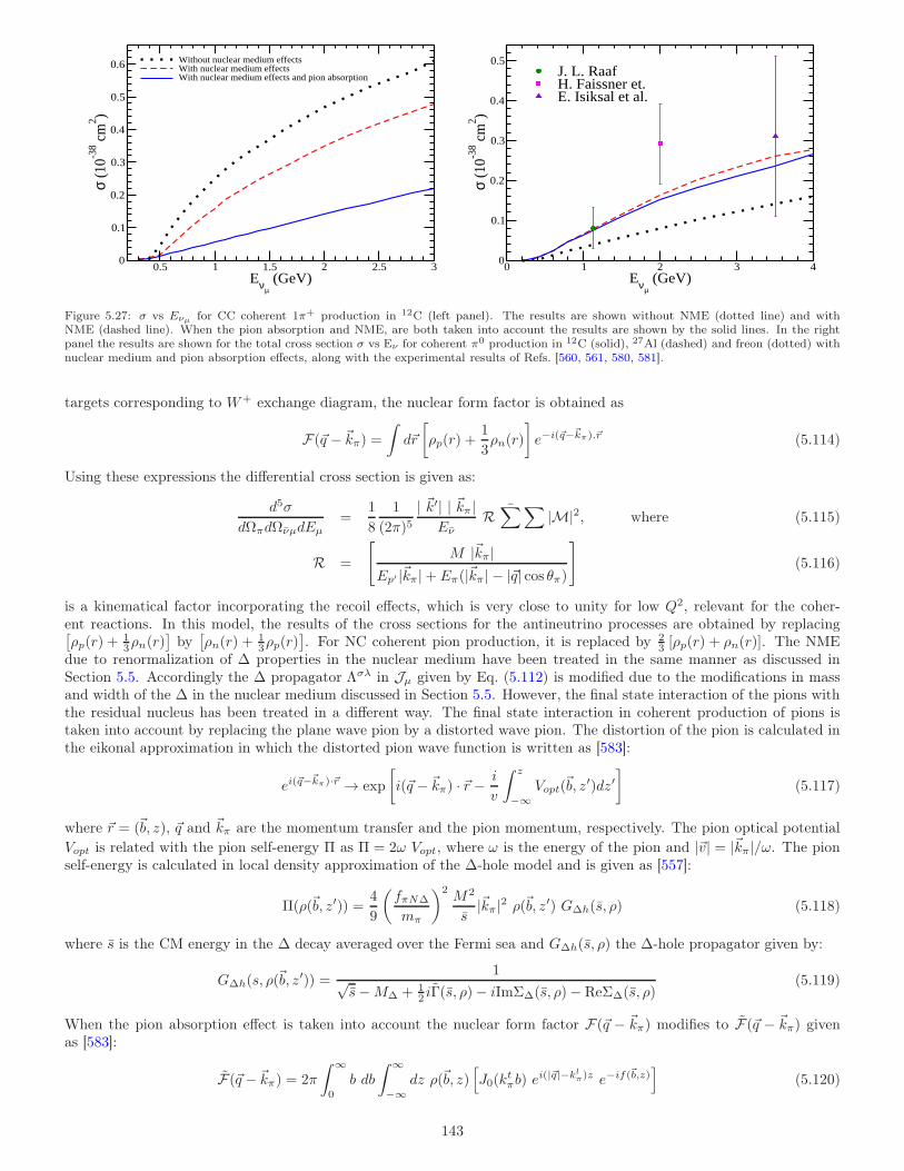
0.5 1 1.5 2 2.5 3Eνµ

(GeV)0

0.1

0.2

0.3

0.4

0.5

0.6

σ (1

0-38 c

m2 )

Without nuclear medium effectsWith nuclear medium effectsWith nuclear medium effects and pion absorption

0 1 2 3 4Eνµ

(GeV)0

0.1

0.2

0.3

0.4

0.5

σ (1

0-38 c

m2 )

J. L. RaafH. Faissner et.E. Isiksal et al.

Figure 5.27: σ vs Eνµ for CC coherent 1π+ production in 12C (left panel). The results are shown without NME (dotted line) and withNME (dashed line). When the pion absorption and NME, are both taken into account the results are shown by the solid lines. In the rightpanel the results are shown for the total cross section σ vs Eν for coherent π0 production in 12C (solid), 27Al (dashed) and freon (dotted) withnuclear medium and pion absorption effects, along with the experimental results of Refs. [560, 561, 580, 581].

targets corresponding to W+ exchange diagram, the nuclear form factor is obtained as

F(~q − ~kπ) =∫

d~r

[

ρp(r) +1

3ρn(r)

]

e−i(~q−~kπ).~r (5.114)

Using these expressions the differential cross section is given as:

d5σ

dΩπdΩνµdEµ=

1

8

1

(2π)5| ~k′| | ~kπ |

EνR ¯∑∑

|M|2, where (5.115)

R =

[

M |~kπ|Ep′ |~kπ|+ Eπ(|~kπ| − |~q| cos θπ)

]

(5.116)

is a kinematical factor incorporating the recoil effects, which is very close to unity for low Q2, relevant for the coher-ent reactions. In this model, the results of the cross sections for the antineutrino processes are obtained by replacing[

ρp(r) +13ρn(r)

]

by[

ρn(r) +13ρp(r)

]

. For NC coherent pion production, it is replaced by 23 [ρp(r) + ρn(r)]. The NME

due to renormalization of ∆ properties in the nuclear medium have been treated in the same manner as discussed inSection 5.5. Accordingly the ∆ propagator Λσλ in Jµ given by Eq. (5.112) is modified due to the modifications in massand width of the ∆ in the nuclear medium discussed in Section 5.5. However, the final state interaction of the pions withthe residual nucleus has been treated in a different way. The final state interaction in coherent production of pions istaken into account by replacing the plane wave pion by a distorted wave pion. The distortion of the pion is calculated inthe eikonal approximation in which the distorted pion wave function is written as [583]:

ei(~q−~kπ)·~r → exp

[

i(~q − ~kπ) · ~r −i

v

∫ z

−∞Vopt(~b, z

′)dz′]

(5.117)

where ~r = (~b, z), ~q and ~kπ are the momentum transfer and the pion momentum, respectively. The pion optical potential

Vopt is related with the pion self-energy Π as Π = 2ω Vopt, where ω is the energy of the pion and |~v| = |~kπ|/ω. The pionself-energy is calculated in local density approximation of the ∆-hole model and is given as [557]:

Π(ρ(~b, z′)) =4

9

(

fπN∆

mπ

)2M2

s|~kπ |2 ρ(~b, z′) G∆h(s, ρ) (5.118)

where s is the CM energy in the ∆ decay averaged over the Fermi sea and G∆h(s, ρ) the ∆-hole propagator given by:

G∆h(s, ρ(~b, z′)) =

1√s−M∆ + 1

2 iΓ(s, ρ)− iImΣ∆(s, ρ)− ReΣ∆(s, ρ)(5.119)

When the pion absorption effect is taken into account the nuclear form factor F(~q − ~kπ) modifies to F(~q − ~kπ) givenas [583]:

F(~q − ~kπ) = 2π

∫ ∞

0

b db

∫ ∞

−∞dz ρ(~b, z)

[

J0(ktπb) e

i(|~q|−klπ)z e−if(~b,z)

]

(5.120)

143

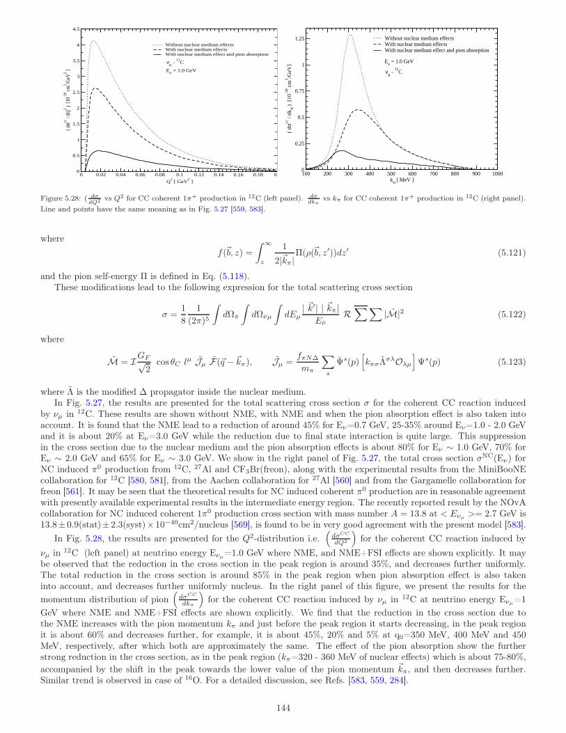
0 0.02 0.04 0.06 0.08 0.1 0.12 0.14 0.16 0.18 0.2

Q2 [ GeV

2 ]

0

0.5

1

1.5

2

2.5

3

3.5

4

4.5

( dσcc

/ dQ

2 ) [1

0-38 c

m2 /G

eV2 ]

Without nuclear medium effectsWith nuclear medium effectsWith nuclear medium effect and pion absorption

Eν = 1.0 GeV

νµ - 12

C

100 200 300 400 500 600 700 800 900 1000kπ [ MeV ]

0

0.25

0.5

0.75

1

1.25

( dσ

cc / d

k π )

[1

0-38 c

m2 /G

eV]

Without nuclear medium effectsWith nuclear medium effectsWith nuclear medium effect and pion absorption

Eν = 1.0 GeV

νµ - 12

C

Figure 5.28: ( dσdQ2 vs Q2 for CC coherent 1π+ production in 12C (left panel). dσ

dkπvs kπ for CC coherent 1π+ production in 12C (right panel).

Line and points have the same meaning as in Fig. 5.27 [559, 583].

where

f(~b, z) =

∫ ∞

z

1

2|~kπ|Π(ρ(~b, z′))dz′ (5.121)

and the pion self-energy Π is defined in Eq. (5.118).These modifications lead to the following expression for the total scattering cross section

σ =1

8

1

(2π)5

∫

dΩπ

∫

dΩνµ

∫

dEµ| ~k′| | ~kπ|

EνR∑∑

|M|2 (5.122)

where

M = IGF√2

cos θC lµ Jµ F(~q − ~kπ), Jµ =fπN∆

mπ

∑

s

Ψs(p)[

kπσΛσλOλµ

]

Ψs(p) (5.123)

where Λ is the modified ∆ propagator inside the nuclear medium.In Fig. 5.27, the results are presented for the total scattering cross section σ for the coherent CC reaction induced

by νµ in 12C. These results are shown without NME, with NME and when the pion absorption effect is also taken intoaccount. It is found that the NME lead to a reduction of around 45% for Eν=0.7 GeV, 25-35% around Eν=1.0 - 2.0 GeVand it is about 20% at Eν=3.0 GeV while the reduction due to final state interaction is quite large. This suppressionin the cross section due to the nuclear medium and the pion absorption effects is about 80% for Eν ∼ 1.0 GeV, 70% forEν ∼ 2.0 GeV and 65% for Eν ∼ 3.0 GeV. We show in the right panel of Fig. 5.27, the total cross section σNC(Eν) forNC induced π0 production from 12C, 27Al and CF3Br(freon), along with the experimental results from the MiniBooNEcollaboration for 12C [580, 581], from the Aachen collaboration for 27Al [560] and from the Gargamelle collaboration forfreon [561]. It may be seen that the theoretical results for NC induced coherent π0 production are in reasonable agreementwith presently available experimental results in the intermediate energy region. The recently reported result by the NOvAcollaboration for NC induced coherent 1π0 production cross section with mass number A = 13.8 at < Eνµ >= 2.7 GeV is13.8± 0.9(stat)± 2.3(syst)× 10−40cm2/nucleus [569], is found to be in very good agreement with the present model [583].

In Fig. 5.28, the results are presented for the Q2-distribution i.e.(

dσCC

dQ2

)

for the coherent CC reaction induced by

νµ in 12C (left panel) at neutrino energy Eνµ=1.0 GeV where NME, and NME+FSI effects are shown explicitly. It maybe observed that the reduction in the cross section in the peak region is around 35%, and decreases further uniformly.The total reduction in the cross section is around 85% in the peak region when pion absorption effect is also takeninto account, and decreases further uniformly nucleus. In the right panel of this figure, we present the results for the

momentum distribution of pion(

dσCC

dkπ

)

for the coherent CC reaction induced by νµ in 12C at neutrino energy Eνµ=1

GeV where NME and NME+FSI effects are shown explicitly. We find that the reduction in the cross section due tothe NME increases with the pion momentum kπ and just before the peak region it starts decreasing, in the peak regionit is about 60% and decreases further, for example, it is about 45%, 20% and 5% at q0=350 MeV, 400 MeV and 450MeV, respectively, after which both are approximately the same. The effect of the pion absorption show the furtherstrong reduction in the cross section, as in the peak region (kπ=320 - 360 MeV of nuclear effects) which is about 75-80%,

accompanied by the shift in the peak towards the lower value of the pion momentum ~kπ, and then decreases further.Similar trend is observed in case of 16O. For a detailed discussion, see Refs. [583, 559, 284].

144

Alvarez-Ruso et al. [585] and Amaro et al. [586] have also included NR contributions (Section 3.3.1) besides the deltaresonance and found the contribution of NR terms to be very small. For the FSI of pion with the nucleus, they solvedthe Klein-Gordon equation. To see the difference in the results obtained by our group [583, 559, 284] and by solvingKlein-Gordon equation for the treatment of pion FSI [585], a comparison was done by Alvarez-Ruso et al. [590] and foundthe difference to be very small. Therefore, while comparing the experimental data for the coherent pion production,Monte Carlo generators generally use the prescription of Ref. [583] for its simplicity.

Nakamura et al. [352] have used dynamical model in coupled channels using the prescription of Ref. [261] where thebare N −∆ transition from a constituent quark model is renormalized by meson clouds. Then the medium modificationof the ∆ properties and pion FSI have been taken into account. They have fitted the free parameters of the scatteringpotential and pion-nucleus optical potential to the pion-nucleus elastic scattering data. For CC process the flux averagedcross section corresponding to K2K experiment was found to be σavg

CC = 6.3×10−40cm2 corresponding to the K2K observedresult of σK2K < 7.7× 10−40cm2 [566]. For NC reaction, the flux averaged cross section for the π0 production calculatedin this model gives σavg

NC = 2.8× 10−40cm2 while the experimentally observed number from the MiniBooNE collaborationis σMiniBooNE = 7.7± 1.6± 3.6× 10−40cm2 [580, 581].

5.7.2. Coherent kaon production

The coherent kaon production has been studied by Alvarez-Ruso et al. [591] using the formalism discussed here inSections 3.6.1 and 3.6.2 for K+ and K− productions respectively. The differential cross section for reaction (3.126) inthe laboratory frame has been taken as:

d 5σ

dΩldk′0dΩK=

1

4(2π)5|~k′||~pK ||~k|M2

G2

2LµνMµ

K+(q, pK) (MνK+(q, pK))

∗. (5.124)

where the nuclear currentMµK+ is obtained as the coherent sum over all nucleons, leading to the nuclear densities

MµK+(q, pK) =

∫

d3~r ei~q·~r

ρp(~r )J µpK+(q, pK) + ρn(~r )J µ

nK+(q, pK)

φ∗>(~pK , ~r). (5.125)

In the above expression

J µNK+(q, pK) =

1

2

∑

i

Tr[

(6 p+M)γ0Γµi;NK+(q, pK)

]M

p0, (5.126)

where the index i refers to all the possible mechanisms in Figs. 3.15 and 3.17; Γµi;NK+ is given in Eq. (3.124) with

jµi = N(p′)Γµi;NK+N(p). The initial and final nucleons in the nucleus, are assumed to be on shell with ~p = (~pK − ~q)/2

and ~p ′ = −~p.φ∗>(~pK , ~r) in Eq. (5.124) denotes the outgoing kaon wave function obtained by solving the Klein-Gordon equation for

the kaons moving in an optical potential Vopt:

(

−~∇2 − ~p 2K + 2p0KVopt

)

φ∗>(~pK , ~r) = 0, (5.127)

Fig. 5.29 shows the results for the coherent K+ and K− production cross sections vs neutrino energy, respectively forνµ(left panel) and νµ(right panel) reaction on 12C nuclear target. Like the νµ induced single kaon production off nucleontarget discussed here in Section 3.6.1, here also the dominant contribution is from the contact term and due to thedestructive interference there is reduction in the total cross sections when all the contributions (Figs 3.15 and 3.17) aretaken into account. It has been observed by these authors [591] that at Eνµ=2GeV, the cross section per nucleon forcarbon nucleus is a factor of about forty smaller than the one obtained for the free nucleon case. Recently MINERvAcollaboration [592] has reported at 3σ C.L., the evidence for coherent kaon production in the neutrino induced scatteringon carbon nuclear target but no real events were reported to be observed.

5.8. Deep inelastic νl/νl − A scattering

5.8.1. Introduction

When a neutrino/antineutrino interacts with a bound nucleon inside a nucleus, the scattering cross sections and thenucleon structure functions get modified due to NME. The reaction for this interaction process via CC DIS channel isrepresented as

νl/νl(k) +A(p) −→ l−/l+(k′) +X(p′) , (5.128)

where A is the target nucleus, X is jet of hadrons in the final state, l = e/µ/τ and the quantities in the parentheses arethe four momenta of the corresponding particles and is shown in Fig. 5.30.

145

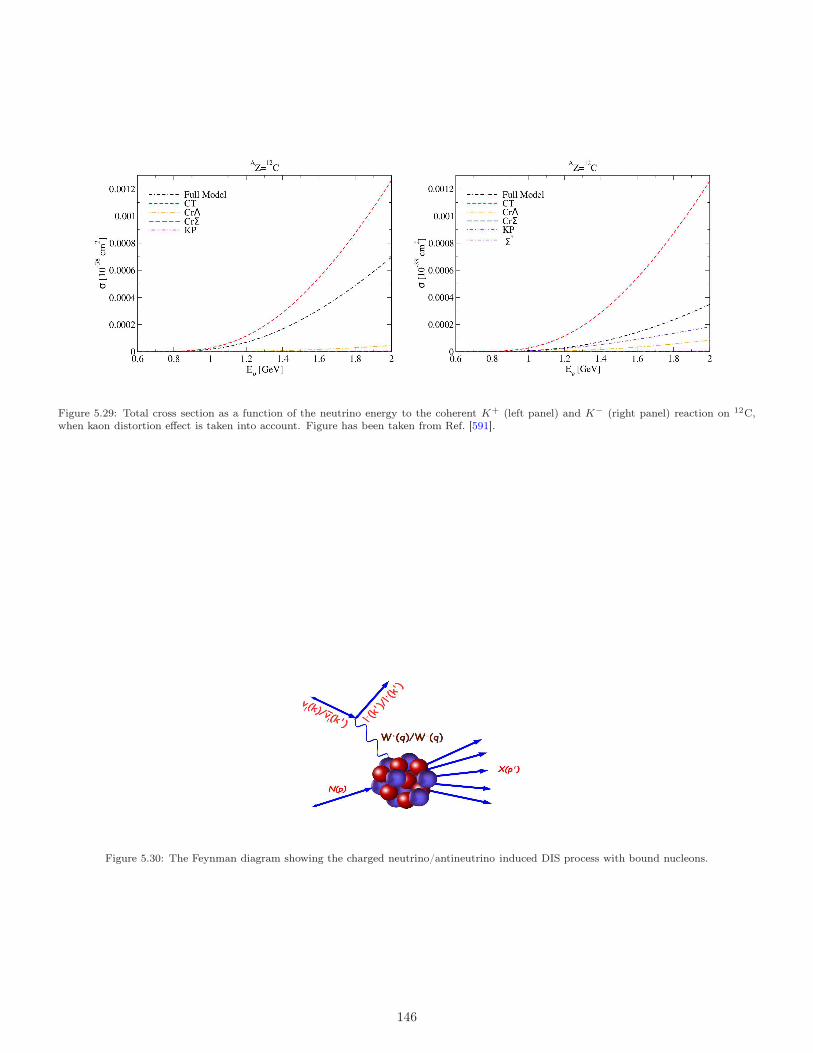
Figure 5.29: Total cross section as a function of the neutrino energy to the coherent K+ (left panel) and K− (right panel) reaction on 12C,when kaon distortion effect is taken into account. Figure has been taken from Ref. [591].

Figure 5.30: The Feynman diagram showing the charged neutrino/antineutrino induced DIS process with bound nucleons.

146

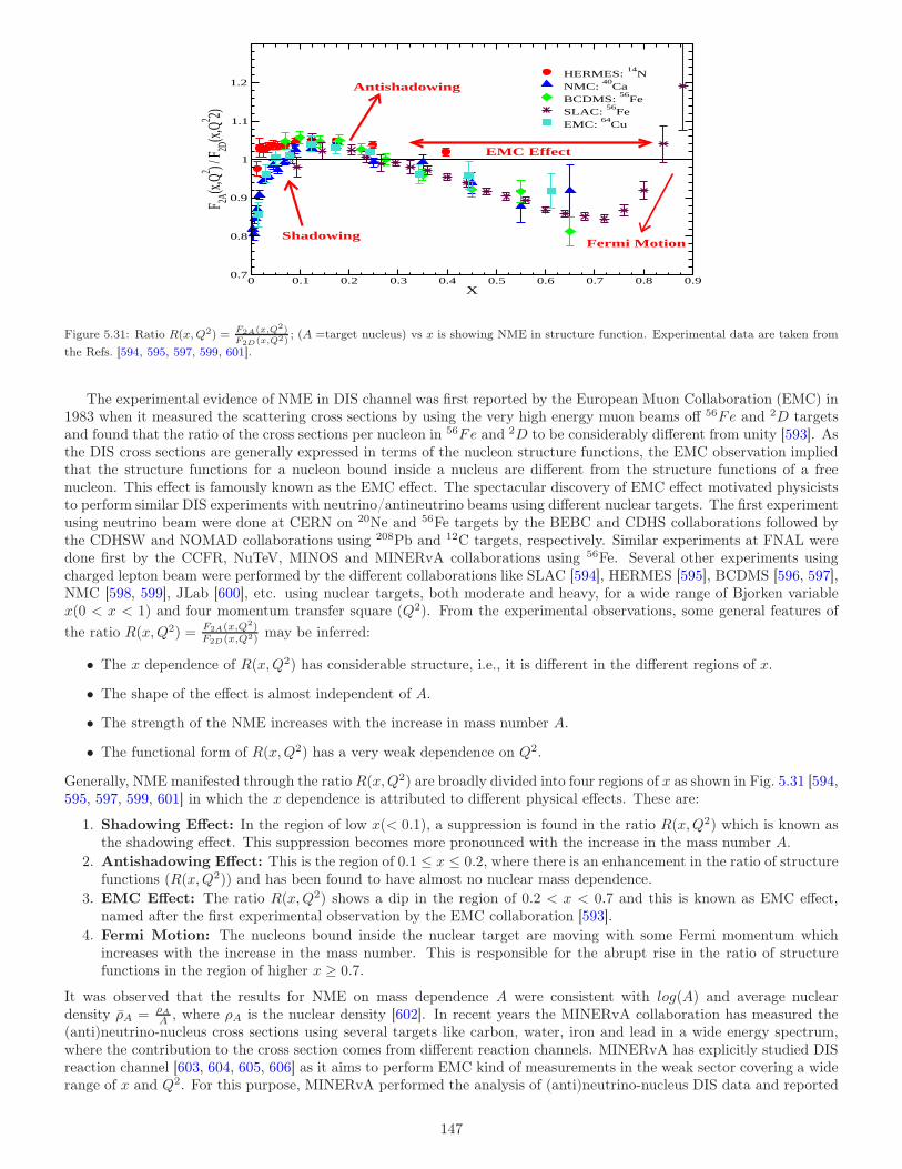
0 0.1 0.2 0.3 0.4 0.5 0.6 0.7 0.8 0.9X

0.7

0.8

0.9

1

1.1

1.2

F 2A(x,

Q2 ) / F 2D

(x,Q2 2)

HERMES: 14

NNMC:

40Ca

BCDMS: 56

FeSLAC:

56Fe

EMC: 64

Cu

Shadowing

Antishadowing

EMC Effect

Fermi Motion

Figure 5.31: Ratio R(x,Q2) = F2A(x,Q2)F2D(x,Q2)

; (A =target nucleus) vs x is showing NME in structure function. Experimental data are taken from

the Refs. [594, 595, 597, 599, 601].

The experimental evidence of NME in DIS channel was first reported by the European Muon Collaboration (EMC) in1983 when it measured the scattering cross sections by using the very high energy muon beams off 56Fe and 2D targetsand found that the ratio of the cross sections per nucleon in 56Fe and 2D to be considerably different from unity [593]. Asthe DIS cross sections are generally expressed in terms of the nucleon structure functions, the EMC observation impliedthat the structure functions for a nucleon bound inside a nucleus are different from the structure functions of a freenucleon. This effect is famously known as the EMC effect. The spectacular discovery of EMC effect motivated physiciststo perform similar DIS experiments with neutrino/antineutrino beams using different nuclear targets. The first experimentusing neutrino beam were done at CERN on 20Ne and 56Fe targets by the BEBC and CDHS collaborations followed bythe CDHSW and NOMAD collaborations using 208Pb and 12C targets, respectively. Similar experiments at FNAL weredone first by the CCFR, NuTeV, MINOS and MINERvA collaborations using 56Fe. Several other experiments usingcharged lepton beam were performed by the different collaborations like SLAC [594], HERMES [595], BCDMS [596, 597],NMC [598, 599], JLab [600], etc. using nuclear targets, both moderate and heavy, for a wide range of Bjorken variablex(0 < x < 1) and four momentum transfer square (Q2). From the experimental observations, some general features of

the ratio R(x,Q2) = F2A(x,Q2)F2D(x,Q2) may be inferred:

• The x dependence of R(x,Q2) has considerable structure, i.e., it is different in the different regions of x.

• The shape of the effect is almost independent of A.

• The strength of the NME increases with the increase in mass number A.

• The functional form of R(x,Q2) has a very weak dependence on Q2.

Generally, NME manifested through the ratio R(x,Q2) are broadly divided into four regions of x as shown in Fig. 5.31 [594,595, 597, 599, 601] in which the x dependence is attributed to different physical effects. These are:

1. Shadowing Effect: In the region of low x(< 0.1), a suppression is found in the ratio R(x,Q2) which is known asthe shadowing effect. This suppression becomes more pronounced with the increase in the mass number A.

2. Antishadowing Effect: This is the region of 0.1 ≤ x ≤ 0.2, where there is an enhancement in the ratio of structurefunctions (R(x,Q2)) and has been found to have almost no nuclear mass dependence.

3. EMC Effect: The ratio R(x,Q2) shows a dip in the region of 0.2 < x < 0.7 and this is known as EMC effect,named after the first experimental observation by the EMC collaboration [593].

4. Fermi Motion: The nucleons bound inside the nuclear target are moving with some Fermi momentum whichincreases with the increase in the mass number. This is responsible for the abrupt rise in the ratio of structurefunctions in the region of higher x ≥ 0.7.

It was observed that the results for NME on mass dependence A were consistent with log(A) and average nucleardensity ρA = ρA

A , where ρA is the nuclear density [602]. In recent years the MINERvA collaboration has measured the(anti)neutrino-nucleus cross sections using several targets like carbon, water, iron and lead in a wide energy spectrum,where the contribution to the cross section comes from different reaction channels. MINERvA has explicitly studied DISreaction channel [603, 604, 605, 606] as it aims to perform EMC kind of measurements in the weak sector covering a widerange of x and Q2. For this purpose, MINERvA performed the analysis of (anti)neutrino-nucleus DIS data and reported

147

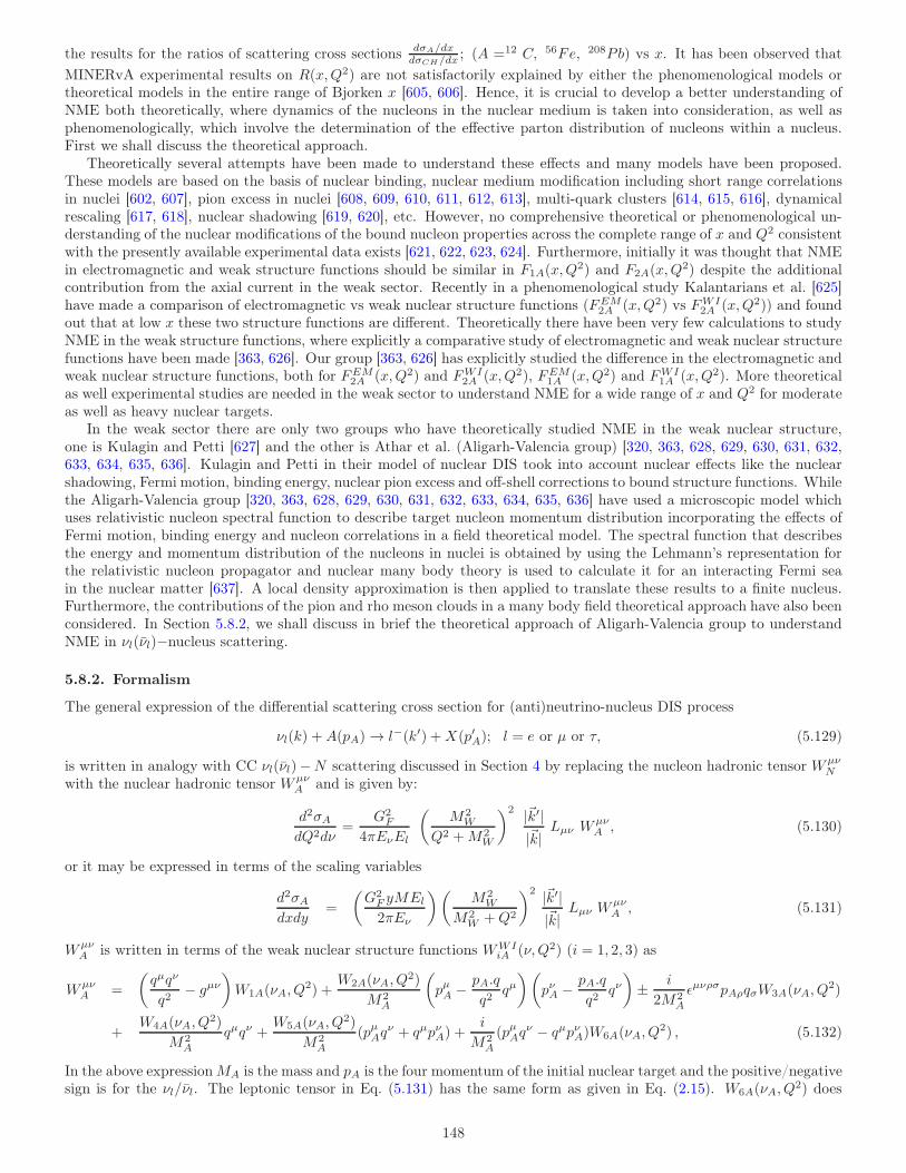
the results for the ratios of scattering cross sections dσA/dxdσCH/dx ; (A =12 C, 56Fe, 208Pb) vs x. It has been observed that

MINERvA experimental results on R(x,Q2) are not satisfactorily explained by either the phenomenological models ortheoretical models in the entire range of Bjorken x [605, 606]. Hence, it is crucial to develop a better understanding ofNME both theoretically, where dynamics of the nucleons in the nuclear medium is taken into consideration, as well asphenomenologically, which involve the determination of the effective parton distribution of nucleons within a nucleus.First we shall discuss the theoretical approach.

Theoretically several attempts have been made to understand these effects and many models have been proposed.These models are based on the basis of nuclear binding, nuclear medium modification including short range correlationsin nuclei [602, 607], pion excess in nuclei [608, 609, 610, 611, 612, 613], multi-quark clusters [614, 615, 616], dynamicalrescaling [617, 618], nuclear shadowing [619, 620], etc. However, no comprehensive theoretical or phenomenological un-derstanding of the nuclear modifications of the bound nucleon properties across the complete range of x and Q2 consistentwith the presently available experimental data exists [621, 622, 623, 624]. Furthermore, initially it was thought that NMEin electromagnetic and weak structure functions should be similar in F1A(x,Q

2) and F2A(x,Q2) despite the additional

contribution from the axial current in the weak sector. Recently in a phenomenological study Kalantarians et al. [625]have made a comparison of electromagnetic vs weak nuclear structure functions (FEM

2A (x,Q2) vs FWI2A (x,Q2)) and found

out that at low x these two structure functions are different. Theoretically there have been very few calculations to studyNME in the weak structure functions, where explicitly a comparative study of electromagnetic and weak nuclear structurefunctions have been made [363, 626]. Our group [363, 626] has explicitly studied the difference in the electromagnetic andweak nuclear structure functions, both for FEM

2A (x,Q2) and FWI2A (x,Q2), FEM

1A (x,Q2) and FWI1A (x,Q2). More theoretical

as well experimental studies are needed in the weak sector to understand NME for a wide range of x and Q2 for moderateas well as heavy nuclear targets.

In the weak sector there are only two groups who have theoretically studied NME in the weak nuclear structure,one is Kulagin and Petti [627] and the other is Athar et al. (Aligarh-Valencia group) [320, 363, 628, 629, 630, 631, 632,633, 634, 635, 636]. Kulagin and Petti in their model of nuclear DIS took into account nuclear effects like the nuclearshadowing, Fermi motion, binding energy, nuclear pion excess and off-shell corrections to bound structure functions. Whilethe Aligarh-Valencia group [320, 363, 628, 629, 630, 631, 632, 633, 634, 635, 636] have used a microscopic model whichuses relativistic nucleon spectral function to describe target nucleon momentum distribution incorporating the effects ofFermi motion, binding energy and nucleon correlations in a field theoretical model. The spectral function that describesthe energy and momentum distribution of the nucleons in nuclei is obtained by using the Lehmann’s representation forthe relativistic nucleon propagator and nuclear many body theory is used to calculate it for an interacting Fermi seain the nuclear matter [637]. A local density approximation is then applied to translate these results to a finite nucleus.Furthermore, the contributions of the pion and rho meson clouds in a many body field theoretical approach have also beenconsidered. In Section 5.8.2, we shall discuss in brief the theoretical approach of Aligarh-Valencia group to understandNME in νl(νl)−nucleus scattering.

5.8.2. Formalism

The general expression of the differential scattering cross section for (anti)neutrino-nucleus DIS process

νl(k) +A(pA)→ l−(k′) +X(p′A); l = e or µ or τ, (5.129)

is written in analogy with CC νl(νl)−N scattering discussed in Section 4 by replacing the nucleon hadronic tensor WµνN

with the nuclear hadronic tensor WµνA and is given by:

d2σAdQ2dν

=G2

F

4πEνEl

(

M2W

Q2 +M2W

)2 |~k′||~k|

Lµν WµνA , (5.130)

or it may be expressed in terms of the scaling variables

d2σAdxdy

=

(

G2F yMEl

2πEν

)(

M2W

M2W +Q2

)2 |~k′||~k|

Lµν WµνA , (5.131)

WµνA is written in terms of the weak nuclear structure functions WWI

iA (ν,Q2) (i = 1, 2, 3) as

WµνA =

(

qµqν

q2− gµν

)

W1A(νA, Q2) +

W2A(νA, Q2)

M2A

(

pµA −pA.q

q2qµ)(

pνA −pA.q

q2qν)

± i

2M2A

ǫµνρσpAρqσW3A(νA, Q2)

+W4A(νA, Q

2)

M2A

qµqν +W5A(νA, Q

2)

M2A

(pµAqν + qµpνA) +

i

M2A

(pµAqν − qµpνA)W6A(νA, Q

2) , (5.132)

In the above expressionMA is the mass and pA is the four momentum of the initial nuclear target and the positive/negativesign is for the νl/νl. The leptonic tensor in Eq. (5.131) has the same form as given in Eq. (2.15). W6A(νA, Q

2) does

148

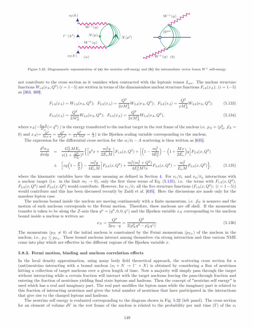
νl(k)

νl(k)

W+(q)

W+(q)

N (p)X(p′)l−(k′)

W+(q)

W+(q)

X

Πµν

(a) (b)

Figure 5.32: Diagrammatic representation of (a) the neutrino self-energy and (b) the intermediate vector boson W+ self-energy.

not contribute to the cross section as it vanishes when contracted with the leptonic tensor Lµν . The nuclear structurefunctions WiA(νA, Q

2) (i = 1−5) are written in terms of the dimensionless nuclear structure functions FiA(xA); (i = 1−5)as [363, 369]:

F1A(xA) =W1A(νA, Q2); F2A(xA) =

Q2

2xM2A

W2A(νA, Q2); F3A(xA) =

Q2

xM2A

W3A(νA, Q2); (5.133)

F4A(xA) =Q2

2M2A

W4A(νA, Q2); F5A(xA) =

Q2

2xM2A

W5A(νA, Q2), (5.134)

where νA(=pA·q

MA

(= q0) ) is the energy transferred to the nuclear target in the rest frame of the nucleus i.e. pA = (p0A, ~pA =

0) and xA(=Q2

2pA·q = Q2

2p0Aq0

= Q2

2A Mq0 = xA ) is the Bjorken scaling variable corresponding to the nucleus.

The expression for the differential cross section for the νl/νl −A scattering is then written as [635]:

d2σAdxdy

=G2

FMEν

π(1 + Q2

M2W

)2

[

y2x+m2

l y

2EνM

]

F1A(x,Q2) +

[(

1− m2l

4E2ν

)

−(

1 +Mx

2Eν

)

y]

F2A(x,Q2)

±[

xy(

1− y

2

)

− m2l y

4EνM

]

F3A(x,Q2) +

m2l (m

2l +Q2)

4E2νM

2xF4A(x,Q

2)− m2l

EνMF5A(x,Q

2)

, (5.135)

where the kinematic variables have the same meaning as defined in Section 4. For νe/νe and νµ/νµ interactions witha nuclear target (i.e. in the limit ml → 0), only the first three terms of Eq. (5.135), i.e. the terms with F1A(x,Q

2),F2A(x,Q

2) and F3A(x,Q2) would contribute. However, for ντ/ντ all the five structure functions (FiA(x,Q

2); (i = 1− 5))would contribute and this has been discussed recently by Zaidi et al. [635]. Here the discussions are made only for themassless lepton case.

The nucleons bound inside the nucleus are moving continuously with a finite momentum, i.e. ~pN is nonzero and themotion of such nucleons corresponds to the Fermi motion. Therefore, these nucleons are off shell. If the momentumtransfer is taken to be along the Z-axis then qµ = (q0, 0, 0, qz) and the Bjorken variable xN corresponding to the nucleonbound inside a nucleus is written as:

xN =Q2

2pN · q=

Q2

2(p0Nq0 − pzNqz)

. (5.136)

The momentum (pN 6= 0) of the initial nucleon is constrained by the Fermi momentum (pFN) of the nucleon in the

nucleus, i.e., pN ≤ pFN. These bound nucleons interact among themselves via strong interaction and thus various NME

come into play which are effective in the different regions of the Bjorken variable x.

5.8.3. Fermi motion, binding and nucleon correlation effects

In the local density approximation, using many body field theoretical approach, the scattering cross section for a(anti)neutrino interacting with a bound nucleon (νl + N → l− + X) is obtained by considering a flux of neutrinoshitting a collection of target nucleons over a given length of time. Now a majority will simply pass through the targetwithout interacting while a certain fraction will interact with the target nucleons leaving the pass-through fraction andentering the fraction of neutrinos yielding final state leptons and hadrons. Then the concept of "neutrino self energy" isused which has a real and imaginary part. The real part modifies the lepton mass while the imaginary part is related tothis fraction of interacting neutrinos and gives the total number of neutrinos that have participated in the interactionsthat give rise to the charged leptons and hadrons.

The neutrino self energy is evaluated corresponding to the diagram shown in Fig. 5.32 (left panel). The cross sectionfor an element of volume dV in the rest frame of the nucleus is related to the probability per unit time (Γ) of the νl

149

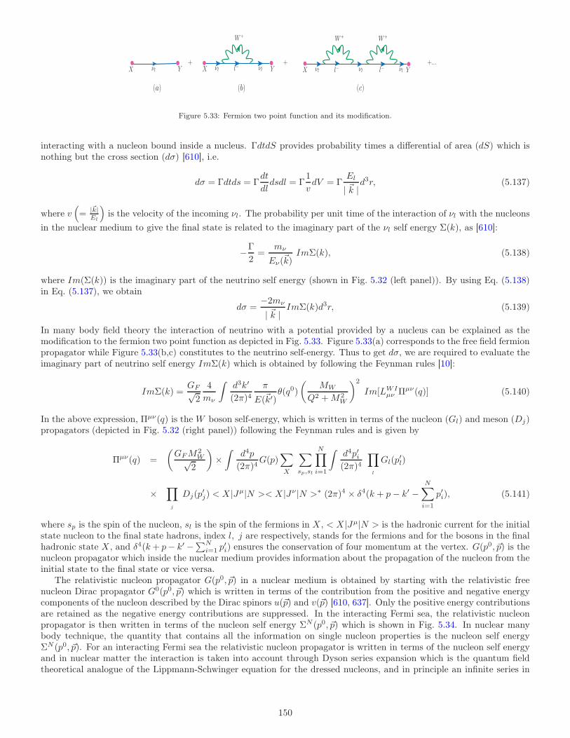
(b)

+

W+

X Yl−νl νl+...

X Yl−νl νl+

νlX Y

(a)

W+ W+

l− νl

(c)

Figure 5.33: Fermion two point function and its modification.

interacting with a nucleon bound inside a nucleus. ΓdtdS provides probability times a differential of area (dS) which isnothing but the cross section (dσ) [610], i.e.

dσ = Γdtds = Γdt

dldsdl = Γ

1

vdV = Γ

El

| ~k |d3r, (5.137)

where v(

= |~k|El

)

is the velocity of the incoming νl. The probability per unit time of the interaction of νl with the nucleons

in the nuclear medium to give the final state is related to the imaginary part of the νl self energy Σ(k), as [610]:

−Γ

2=

mν

Eν(~k)ImΣ(k), (5.138)

where Im(Σ(k)) is the imaginary part of the neutrino self energy (shown in Fig. 5.32 (left panel)). By using Eq. (5.138)in Eq. (5.137), we obtain

dσ =−2mν

| ~k |ImΣ(k)d3r, (5.139)

In many body field theory the interaction of neutrino with a potential provided by a nucleus can be explained as themodification to the fermion two point function as depicted in Fig. 5.33. Figure 5.33(a) corresponds to the free field fermionpropagator while Figure 5.33(b,c) constitutes to the neutrino self-energy. Thus to get dσ, we are required to evaluate theimaginary part of neutrino self energy ImΣ(k) which is obtained by following the Feynman rules [10]:

ImΣ(k) =GF√2

4

mν

∫

d3k′

(2π)4π

E(~k′)θ(q0)

(

MW

Q2 +M2W

)2

Im[LWIµν Πµν(q)] (5.140)

In the above expression, Πµν(q) is the W boson self-energy, which is written in terms of the nucleon (Gl) and meson (Dj)propagators (depicted in Fig. 5.32 (right panel)) following the Feynman rules and is given by

Πµν(q) =

(

GFM2W√

2

)

×∫

d4p

(2π)4G(p)

∑

X

∑

sp,sl

N∏

i=1

∫

d4p′i(2π)4

∏

l

Gl(p′l)

×∏

j

Dj(p′j) < X |Jµ|N >< X |Jν |N >∗ (2π)4 × δ4(k + p− k′ −

N∑

i=1

p′i), (5.141)

where sp is the spin of the nucleon, sl is the spin of the fermions in X , < X |Jµ|N > is the hadronic current for the initialstate nucleon to the final state hadrons, index l, j are respectively, stands for the fermions and for the bosons in the finalhadronic state X , and δ4(k+ p− k′ −∑N

i=1 p′i) ensures the conservation of four momentum at the vertex. G(p0, ~p) is the

nucleon propagator which inside the nuclear medium provides information about the propagation of the nucleon from theinitial state to the final state or vice versa.

The relativistic nucleon propagator G(p0, ~p) in a nuclear medium is obtained by starting with the relativistic freenucleon Dirac propagator G0(p0, ~p) which is written in terms of the contribution from the positive and negative energycomponents of the nucleon described by the Dirac spinors u(~p) and v(~p) [610, 637]. Only the positive energy contributionsare retained as the negative energy contributions are suppressed. In the interacting Fermi sea, the relativistic nucleonpropagator is then written in terms of the nucleon self energy ΣN (p0, ~p) which is shown in Fig. 5.34. In nuclear manybody technique, the quantity that contains all the information on single nucleon properties is the nucleon self energyΣN (p0, ~p). For an interacting Fermi sea the relativistic nucleon propagator is written in terms of the nucleon self energyand in nuclear matter the interaction is taken into account through Dyson series expansion which is the quantum fieldtheoretical analogue of the Lippmann-Schwinger equation for the dressed nucleons, and in principle an infinite series in

150

+ + + +.............

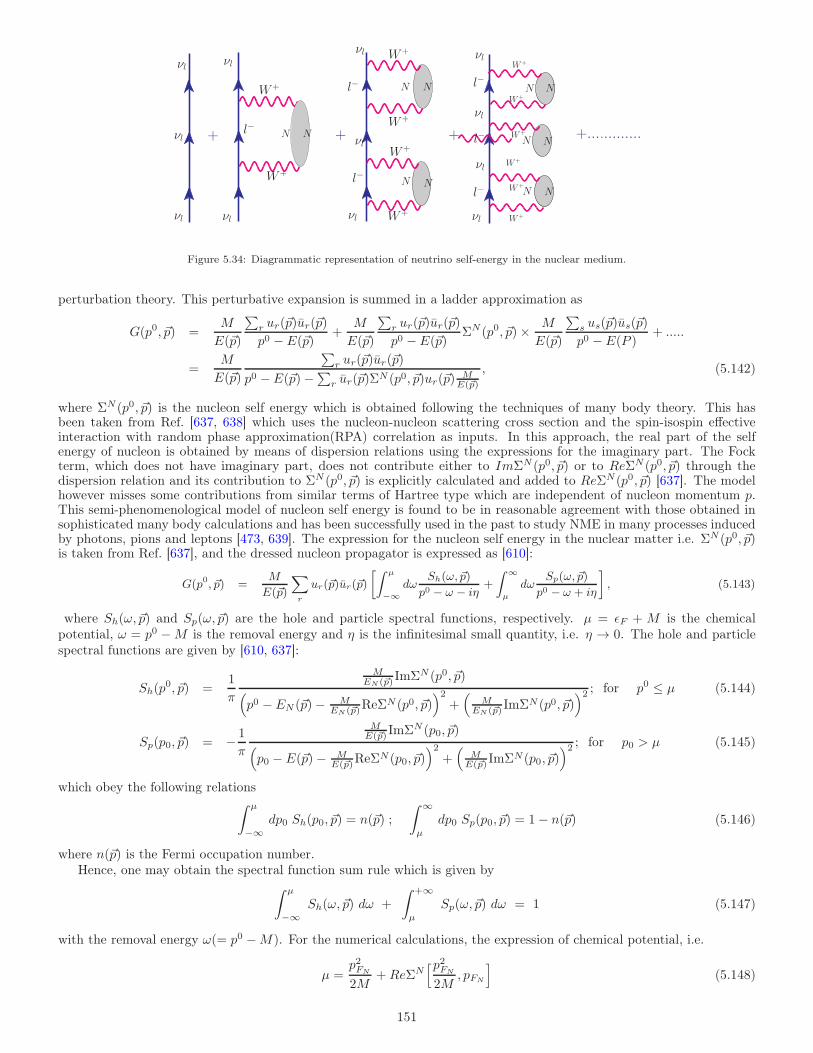
νl νlνlνl

νl

νl

l−

νl

W+

W+

N

l−

νl

l−

νl W+

W+

W+

W+

N

Nl−

νl

N

N

N

l−

νl

l−

νl

W+

W+N N

W+

W+

N N

W+

W+

N N

Figure 5.34: Diagrammatic representation of neutrino self-energy in the nuclear medium.

perturbation theory. This perturbative expansion is summed in a ladder approximation as

G(p0, ~p) =M

E(~p)

∑

r ur(~p)ur(~p)

p0 − E(~p)+

M

E(~p)

∑

r ur(~p)ur(~p)

p0 − E(~p)ΣN (p0, ~p)× M

E(~p)

∑

s us(~p)us(~p)

p0 − E(P )+ .....

=M

E(~p)

∑

r ur(~p)ur(~p)

p0 − E(~p)−∑r ur(~p)ΣN (p0, ~p)ur(~p)

ME(~p)

, (5.142)

where ΣN (p0, ~p) is the nucleon self energy which is obtained following the techniques of many body theory. This hasbeen taken from Ref. [637, 638] which uses the nucleon-nucleon scattering cross section and the spin-isospin effectiveinteraction with random phase approximation(RPA) correlation as inputs. In this approach, the real part of the selfenergy of nucleon is obtained by means of dispersion relations using the expressions for the imaginary part. The Fockterm, which does not have imaginary part, does not contribute either to ImΣN (p0, ~p) or to ReΣN (p0, ~p) through thedispersion relation and its contribution to ΣN (p0, ~p) is explicitly calculated and added to ReΣN(p0, ~p) [637]. The modelhowever misses some contributions from similar terms of Hartree type which are independent of nucleon momentum p.This semi-phenomenological model of nucleon self energy is found to be in reasonable agreement with those obtained insophisticated many body calculations and has been successfully used in the past to study NME in many processes inducedby photons, pions and leptons [473, 639]. The expression for the nucleon self energy in the nuclear matter i.e. ΣN (p0, ~p)is taken from Ref. [637], and the dressed nucleon propagator is expressed as [610]:

G(p0, ~p) =M

E(~p)

∑

r

ur(~p)ur(~p)

[∫ µ

−∞dω

Sh(ω, ~p)

p0 − ω − iη+

∫ ∞

µ

dωSp(ω, ~p)

p0 − ω + iη

]

, (5.143)

where Sh(ω, ~p) and Sp(ω, ~p) are the hole and particle spectral functions, respectively. µ = ǫF + M is the chemicalpotential, ω = p0 −M is the removal energy and η is the infinitesimal small quantity, i.e. η → 0. The hole and particlespectral functions are given by [610, 637]:

Sh(p0, ~p) =

1

π

MEN (~p) ImΣN (p0, ~p)

(

p0 − EN (~p)− MEN (~p)ReΣN (p0, ~p)

)2

+(

MEN (~p) ImΣN (p0, ~p)

)2 ; for p0 ≤ µ (5.144)

Sp(p0, ~p) = − 1

π

ME(~p) ImΣN (p0, ~p)

(

p0 − E(~p)− ME(~p)ReΣN (p0, ~p)

)2

+(

ME(~p) ImΣN (p0, ~p)

)2 ; for p0 > µ (5.145)

which obey the following relations∫ µ

−∞dp0 Sh(p0, ~p) = n(~p) ;

∫ ∞

µ

dp0 Sp(p0, ~p) = 1− n(~p) (5.146)

where n(~p) is the Fermi occupation number.Hence, one may obtain the spectral function sum rule which is given by

∫ µ

−∞Sh(ω, ~p) dω +

∫ +∞

µ

Sp(ω, ~p) dω = 1 (5.147)

with the removal energy ω(= p0 −M). For the numerical calculations, the expression of chemical potential, i.e.

µ =p2FN

2M+ReΣN

[p2FN

2M,pFN

]

(5.148)

151

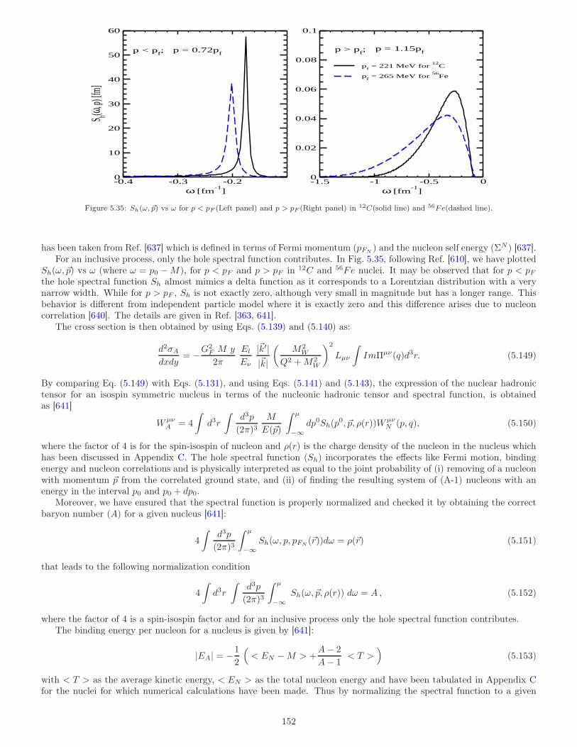
-0.4 -0.3 -0.2ω [fm

-1]

0

10

20

30

40

50

60

S h(ω, p)

[fm]

pf = 221 MeV for

12C

pf = 265 MeV for

56Fe

-1.5 -1 -0.5 0ω [fm

-1]

0

0.02

0.04

0.06

0.08

0.1

p < pf; p > p

f; p = 1.15p

fp = 0.72pf

Figure 5.35: Sh(ω, ~p) vs ω for p < pF (Left panel) and p > pF (Right panel) in 12C(solid line) and 56Fe(dashed line).

has been taken from Ref. [637] which is defined in terms of Fermi momentum (pFN) and the nucleon self energy (ΣN ) [637].

For an inclusive process, only the hole spectral function contributes. In Fig. 5.35, following Ref. [610], we have plottedSh(ω, ~p) vs ω (where ω = p0 −M), for p < pF and p > pF in 12C and 56Fe nuclei. It may be observed that for p < pFthe hole spectral function Sh almost mimics a delta function as it corresponds to a Lorentzian distribution with a verynarrow width. While for p > pF , Sh is not exactly zero, although very small in magnitude but has a longer range. Thisbehavior is different from independent particle model where it is exactly zero and this difference arises due to nucleoncorrelation [640]. The details are given in Ref. [363, 641].

The cross section is then obtained by using Eqs. (5.139) and (5.140) as:

d2σAdxdy

= −G2F M y

2π

El

Eν

|~k′||~k|

(

M2W

Q2 +M2W

)2

Lµν

∫

ImΠµν(q)d3r. (5.149)

By comparing Eq. (5.149) with Eqs. (5.131), and using Eqs. (5.141) and (5.143), the expression of the nuclear hadronictensor for an isospin symmetric nucleus in terms of the nucleonic hadronic tensor and spectral function, is obtainedas [641]

WµνA = 4

∫

d3r

∫

d3p

(2π)3M

E(~p)

∫ µ

−∞dp0Sh(p

0, ~p, ρ(r))WµνN (p, q), (5.150)

where the factor of 4 is for the spin-isospin of nucleon and ρ(r) is the charge density of the nucleon in the nucleus whichhas been discussed in Appendix C. The hole spectral function (Sh) incorporates the effects like Fermi motion, bindingenergy and nucleon correlations and is physically interpreted as equal to the joint probability of (i) removing of a nucleonwith momentum ~p from the correlated ground state, and (ii) of finding the resulting system of (A-1) nucleons with anenergy in the interval p0 and p0 + dp0.

Moreover, we have ensured that the spectral function is properly normalized and checked it by obtaining the correctbaryon number (A) for a given nucleus [641]:

4

∫

d3p

(2π)3

∫ µ

−∞Sh(ω, p, pFN

(~r))dω = ρ(~r) (5.151)

that leads to the following normalization condition

4

∫

d3r

∫

d3p

(2π)3

∫ µ

−∞Sh(ω, ~p, ρ(r)) dω = A , (5.152)

where the factor of 4 is a spin-isospin factor and for an inclusive process only the hole spectral function contributes.The binding energy per nucleon for a nucleus is given by [641]:

|EA| = −1

2

(

< EN −M > +A− 2

A− 1< T >

)

(5.153)

with < T > as the average kinetic energy, < EN > as the total nucleon energy and have been tabulated in Appendix Cfor the nuclei for which numerical calculations have been made. Thus by normalizing the spectral function to a given

152

number of nucleons in the nucleus and getting a binding energy very close to the experimental value, no free parameteris left. Details are given in Ref. [637, 641].

However, for a nonisoscalar nuclear targetWµνA is written in terms of the proton/neutron hole spectral function (Sj

h; j =p, n) and the corresponding hadronic tensor (Wµν

j ; j = p, n) as

WµνA = 2

∑

j=p,n

∫

d3r

∫

d3p

(2π)3M

EN (~p)

∫ µj

−∞dp0Sj

h(p0, ~p, ρ(r))Wµν

j (p, q), (5.154)

where the factor of 2 is due to the two possible projections of nucleon spin and µj ; (j = p, n) is the chemical potentialfor the proton/neutron. In the local density approximation, the hole spectral functions of protons and neutrons are thefunction of local Fermi momentum and the equivalent normalization is written as

2

∫

d3p

(2π)3

∫ µ

−∞Sp,nh (ω, p, pFp,n

(~r))dω = ρp,n(~r) (5.155)

pFp(n)is the Fermi momentum of proton/neutron inside the nucleus which is expressed in terms of the proton/neutron

density as discussed above. The hole spectral functions are normalized separately to the respective proton and neutronnumbers in a nuclear target as [363, 641]:

2

∫

d3r

∫

d3p

(2π)3

∫ µp

−∞Sph(ω, ~p, ρp(r)) dω = Z , (5.156)

2

∫

d3r

∫

d3p

(2π)3

∫ µn

−∞Snh (ω, ~p, ρn(r)) dω = N . (5.157)

The hadronic tensor (Wµνj ) is then written in terms of the dimensionless proton and neutron structure functions (Fij(x,Q

2);i = 1 − 5; j = p, n). By using Eq. (5.154) and the general form of hadronic tensor with an appropriate choice of x, y, zcomponents, we obtain the following expressions of dimensionless nuclear structure functions for a nonisoscalar nucleartarget [362, 363, 641]:

FiA,N (xA, Q2) = 4

∫

d3r

∫

d3p

(2π)3M

EN (~p)

∫ µ

−∞dp0 Sh(p

0, ~p, ρ(r)) × fiN (x,Q2) (5.158)

where i = 1− 5 and

f1N (x,Q2) = AM

[

F1N (xN , Q2)

M+

(

px

M

)2F2N (xN , Q

2)

νN

]

, (5.159)

f2N (x,Q2) =

(

F2N (xN , Q2)

M2νN

)

[

Q4

q0(qz)2

(

pz +q0(p0 − γpz)

Q2qz)2

+q0Q2(px)2

(qz)2

]

(5.160)

f3N (x,Q2) = Aq0

qz×(

p0qz − pzq0p · q

)

F3N (xN , Q2), (5.161)

f4N (x,Q2) = A

[

F4N (xN , Q2) +

pzQ2

qzF5N (x,Q2)

MνN

]

, (5.162)

f5N (x,Q2) = AF5N (xN , Q

2)

MνN×[

q0(p0 − γpz) +Q2 pz

qz

]

(5.163)

where νN = p·qM = p0q0−pzqz

M , γ = q0

qz . Using these expressions, the effect of Fermi motion, binding energy and nucleoncorrelations have been included through the use of hole spectral function. Furthermore, bound nucleons may interactwith each other via meson exchange such as π, ρ, etc., and the interaction of the intermediate vector boson with themesons play an important role in the evaluation of nuclear structure functions [363, 632]. Hence, we have incorporatedthese effects in the numerical calculations and discussed the mesonic contributions in the following Section 5.8.4.

5.8.4. Mesonic contributions

There are virtual mesons (mainly π and ρ mesons) associated with each nucleon bound inside the nucleus. This mesoniccloud gets strengthened by the strong attractive nature of the nucleon-nucleon interaction, which leads to a reasonablygood probability of interaction of virtual bosons(IVB) with a meson instead of a nucleon [610, 611, 642, 643]. It has beenobserved by us that the mesonic contribution, which is mainly dominated by the pion cloud, becomes more pronounced

153

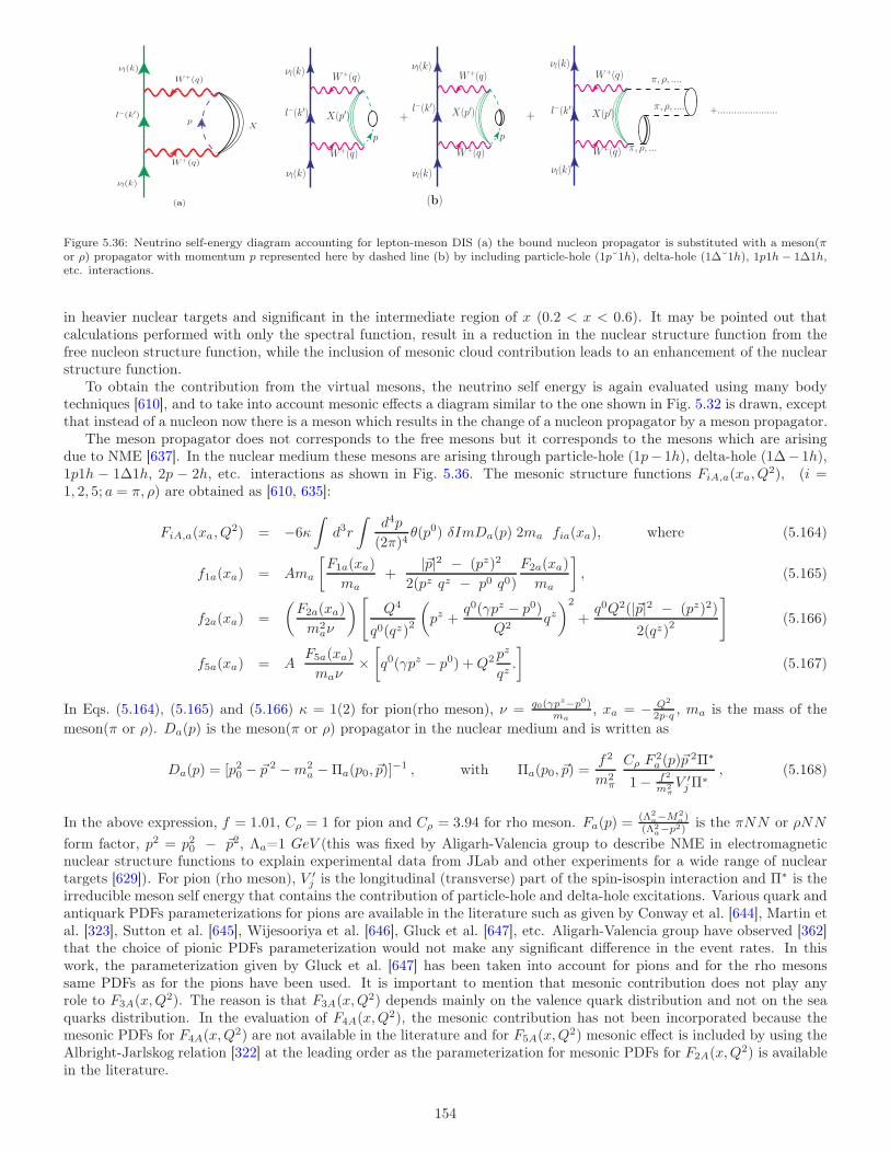
νl(k)

l−(k′)

νl(k)

W+(q)

W+(q)

pX

(a)

X(p′) +

νl(k)

l−(k′)

νl(k) W+(q)

W+(q)

p

+l−(k′)

p

X(p′)

νl(k)

νl(k)W+(q)

W+(q)

νl(k)

νl(k)W+(q)

W+(q)

l−(k′) X(p′) +......................

π, ρ, ...

π, ρ, ....

π, ρ, ....

(b)

Figure 5.36: Neutrino self-energy diagram accounting for lepton-meson DIS (a) the bound nucleon propagator is substituted with a meson(πor ρ) propagator with momentum p represented here by dashed line (b) by including particle-hole (1p˘1h), delta-hole (1∆˘1h), 1p1h− 1∆1h,etc. interactions.

in heavier nuclear targets and significant in the intermediate region of x (0.2 < x < 0.6). It may be pointed out thatcalculations performed with only the spectral function, result in a reduction in the nuclear structure function from thefree nucleon structure function, while the inclusion of mesonic cloud contribution leads to an enhancement of the nuclearstructure function.

To obtain the contribution from the virtual mesons, the neutrino self energy is again evaluated using many bodytechniques [610], and to take into account mesonic effects a diagram similar to the one shown in Fig. 5.32 is drawn, exceptthat instead of a nucleon now there is a meson which results in the change of a nucleon propagator by a meson propagator.

The meson propagator does not corresponds to the free mesons but it corresponds to the mesons which are arisingdue to NME [637]. In the nuclear medium these mesons are arising through particle-hole (1p− 1h), delta-hole (1∆− 1h),1p1h − 1∆1h, 2p − 2h, etc. interactions as shown in Fig. 5.36. The mesonic structure functions FiA,a(xa, Q

2), (i =1, 2, 5; a = π, ρ) are obtained as [610, 635]:

FiA,a(xa, Q2) = −6κ

∫

d3r

∫

d4p

(2π)4θ(p0) δImDa(p) 2ma fia(xa), where (5.164)

f1a(xa) = Ama

[

F1a(xa)

ma+

|~p|2 − (pz)2

2(pz qz − p0 q0)

F2a(xa)

ma

]

, (5.165)

f2a(xa) =

(

F2a(xa)

m2aν

)

[

Q4

q0(qz)2

(

pz +q0(γpz − p0)

Q2qz)2

+q0Q2(|~p|2 − (pz)2)

2(qz)2

]

(5.166)

f5a(xa) = AF5a(xa)

maν×[

q0(γpz − p0) +Q2 pz

qz.

]

(5.167)

In Eqs. (5.164), (5.165) and (5.166) κ = 1(2) for pion(rho meson), ν = q0(γpz−p0)

ma, xa = − Q2

2p·q , ma is the mass of the

meson(π or ρ). Da(p) is the meson(π or ρ) propagator in the nuclear medium and is written as

Da(p) = [p20 − ~p 2 −m2a −Πa(p0, ~p)]

−1 , with Πa(p0, ~p) =f2

m2π

Cρ F2a (p)~p

2Π∗

1− f2

m2πV ′jΠ

∗, (5.168)

In the above expression, f = 1.01, Cρ = 1 for pion and Cρ = 3.94 for rho meson. Fa(p) =(Λ2

a−M2a)

(Λ2a−p2) is the πNN or ρNN

form factor, p2 = p20 − ~p2, Λa=1 GeV (this was fixed by Aligarh-Valencia group to describe NME in electromagneticnuclear structure functions to explain experimental data from JLab and other experiments for a wide range of nucleartargets [629]). For pion (rho meson), V ′

j is the longitudinal (transverse) part of the spin-isospin interaction and Π∗ is theirreducible meson self energy that contains the contribution of particle-hole and delta-hole excitations. Various quark andantiquark PDFs parameterizations for pions are available in the literature such as given by Conway et al. [644], Martin etal. [323], Sutton et al. [645], Wijesooriya et al. [646], Gluck et al. [647], etc. Aligarh-Valencia group have observed [362]that the choice of pionic PDFs parameterization would not make any significant difference in the event rates. In thiswork, the parameterization given by Gluck et al. [647] has been taken into account for pions and for the rho mesonssame PDFs as for the pions have been used. It is important to mention that mesonic contribution does not play anyrole to F3A(x,Q

2). The reason is that F3A(x,Q2) depends mainly on the valence quark distribution and not on the sea

quarks distribution. In the evaluation of F4A(x,Q2), the mesonic contribution has not been incorporated because the

mesonic PDFs for F4A(x,Q2) are not available in the literature and for F5A(x,Q

2) mesonic effect is included by using theAlbright-Jarlskog relation [322] at the leading order as the parameterization for mesonic PDFs for F2A(x,Q

2) is availablein the literature.

154

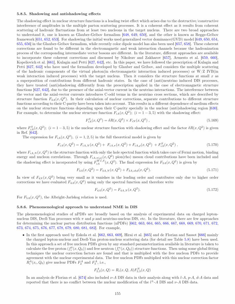
5.8.5. Shadowing and antishadowing effects

The shadowing effect in nuclear structure functions is a leading twist effect which arises due to the destructive/constructiveinterference of amplitudes in the multiple parton scattering processes. It is a coherent effect as it results from coherentscattering of hadronic fluctuations from at least two nucleons in the target nucleus. There are two broad approachesto understand it, one is known as Glauber-Gribov formalism [648, 649, 650], and the other is known as Regge-Gribovframework [651, 652, 653]. For shadowing the initial works used generalized vector dominance(GVD) model [649, 650, 654,655, 656] in the Glauber-Gribov formalism, while recently color dipole model has also been used [657, 658]. These coherentcorrections are found to be different in the electromagnetic and weak interaction channels because the hadronizationprocess of the corresponding intermediate vector bosons are different. In the literature, different approaches are availableto incorporate these coherent corrections and discussed by Nikoleav and Zakharov [657], Armesto et al. [659, 660],Kopeliovich et al. [661], Kulagin and Petti [627, 642], etc. In this paper, we have followed the prescription of Kulagin andPetti [627, 642] who have used the formalism developed by Glauber and Gribov, and considers the multiple scatteringof the hadronic components of the virtual photon(in electromagnetic interaction induced processes) or W/Z IVB(inweak interaction induced processes) with the target nucleus. Then it considers the structure functions at small x asa superposition of contributions from different hadronic states. In the case of (anti)neutrino induced DIS processes,they have treated (anti)shadowing differently from the prescription applied in the case of electromagnetic structurefunctions [627, 642], due to the presence of the axial-vector current in the neutrino interactions. The interference betweenthe vector and the axial-vector currents introduces C-odd terms in the neutrino cross sections, which are described bystructure function F3A(x,Q

2). In their calculation of nuclear corrections, separate contributions to different structurefunctions according to their C-parity have been taken into account. This results in a different dependence of medium effectson the nuclear structure functions depending upon their C-parity specially in the nuclear (anti)shadowing region [630].For example, to determine the nuclear structure function FiA(x,Q

2); (i = 1− 3, 5) with the shadowing effect:

FSiA(x,Q

2) = δR(x,Q2)× FiN (x,Q2) , (5.169)

where FSiA(x,Q

2); (i = 1− 3, 5) is the nuclear structure function with shadowing effect and the factor δR(x,Q2) is givenin Ref. [642].

The expression for FiA(x,Q2), (i = 1, 2, 5) in the full theoretical model is given by

FiA(x,Q2) = FiA,N (x,Q2) + FiA,π(x,Q

2) + FiA,ρ(x,Q2) + FS

iA(x,Q2) , (5.170)

where FiA,N (x,Q2) is the structure function with only the hole spectral function which takes care of Fermi motion, bindingenergy and nucleon correlations. Through FiA,π(ρ)(x,Q

2) pion(rho) meson cloud contributions have been included and

the shadowing effect is incorporated by using FWI,SiA (x,Q2). The final expression for F3A(x,Q

2) is given by

F3A(x,Q2) = F3A,N (x,Q2) + F3A,shd(x,Q

2). (5.171)

In view of F4N (x,Q2) being very small as it vanishes in the leading order and contributes only due to higher ordercorrections we have evaluated F4A(x,Q

2) using only the spectral function and therefore write

F4A(x,Q2) = F4A,N (x,Q2). (5.172)

For F5A(x,Q2), the Albright-Jarlskog relation is used.

5.8.6. Phenomenological approach to understand NME in DIS

The phenomenological studies of nPDFs are broadly based on the analysis of experimental data on charged lepton-nucleus DIS, Drell-Yan processes with π and p and neutrino-nucleus DIS, etc. In the literature, there are few approachesfor determining the nuclear parton distribution functions (nPDFs) [662, 663, 664, 665, 666, 667, 668, 669, 670, 671, 672,673, 674, 675, 676, 677, 678, 679, 680, 681, 682]. For example,

• In the first approach used by Eskola et al. [662, 663, 669], Hirai et al. [665] and de Florian and Sassot [666] mainlythe charged lepton-nucleus and Drell-Yan proton-nucleus scattering data (for detail see Table 5.8) have been used.In this approach a set of free nucleon PDFs given by any standard parameterization available in literature is taken tocalculate the free proton (fp

i (x,Q0)) and free neutron (fni (x,Q0)) structure functions. Then using some global fitting

techniques the nuclear correction factors are found and that is multiplied with the free nucleon PDFs to provideagreement with the nuclear experimental data. The free nucleon PDFs multiplied with this nuclear correction factorRA

i (xi, Q0) give nuclear PDFs FA2 and FA

3 , i.e.,

FA2,3(x,Q) = Ri(x,Q,A)F

N2,3(x,Q)

In an analysis de Florian et al. [674] also included ν-A DIS data in their analysis along with l-A, p-A, d-A data andreported that there is no conflict between the nuclear modification of the l±-A DIS and ν-A DIS data.

155

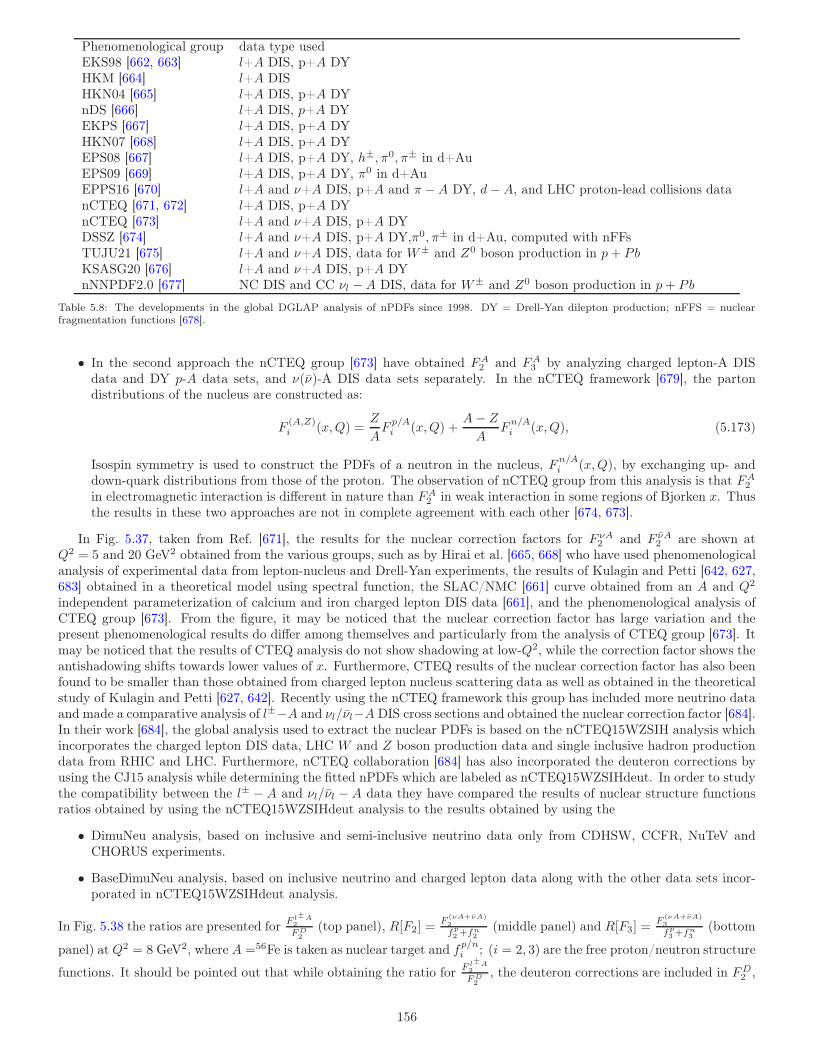
Phenomenological group data type usedEKS98 [662, 663] l+A DIS, p+A DYHKM [664] l+A DISHKN04 [665] l+A DIS, p+A DYnDS [666] l+A DIS, p+A DYEKPS [667] l+A DIS, p+A DYHKN07 [668] l+A DIS, p+A DYEPS08 [667] l+A DIS, p+A DY, h±, π0, π± in d+AuEPS09 [669] l+A DIS, p+A DY, π0 in d+AuEPPS16 [670] l+A and ν+A DIS, p+A and π −A DY, d−A, and LHC proton-lead collisions datanCTEQ [671, 672] l+A DIS, p+A DYnCTEQ [673] l+A and ν+A DIS, p+A DYDSSZ [674] l+A and ν+A DIS, p+A DY,π0, π± in d+Au, computed with nFFsTUJU21 [675] l+A and ν+A DIS, data for W± and Z0 boson production in p+ PbKSASG20 [676] l+A and ν+A DIS, p+A DYnNNPDF2.0 [677] NC DIS and CC νl −A DIS, data for W± and Z0 boson production in p+ Pb

Table 5.8: The developments in the global DGLAP analysis of nPDFs since 1998. DY = Drell-Yan dilepton production; nFFS = nuclearfragmentation functions [678].

• In the second approach the nCTEQ group [673] have obtained FA2 and FA

3 by analyzing charged lepton-A DISdata and DY p-A data sets, and ν(ν)-A DIS data sets separately. In the nCTEQ framework [679], the partondistributions of the nucleus are constructed as:

F(A,Z)i (x,Q) =

Z

AF

p/Ai (x,Q) +

A− ZA

Fn/Ai (x,Q), (5.173)

Isospin symmetry is used to construct the PDFs of a neutron in the nucleus, Fn/Ai (x,Q), by exchanging up- and

down-quark distributions from those of the proton. The observation of nCTEQ group from this analysis is that FA2

in electromagnetic interaction is different in nature than FA2 in weak interaction in some regions of Bjorken x. Thus

the results in these two approaches are not in complete agreement with each other [674, 673].

In Fig. 5.37, taken from Ref. [671], the results for the nuclear correction factors for F νA2 and F νA

2 are shown atQ2 = 5 and 20 GeV2 obtained from the various groups, such as by Hirai et al. [665, 668] who have used phenomenologicalanalysis of experimental data from lepton-nucleus and Drell-Yan experiments, the results of Kulagin and Petti [642, 627,683] obtained in a theoretical model using spectral function, the SLAC/NMC [661] curve obtained from an A and Q2

independent parameterization of calcium and iron charged lepton DIS data [661], and the phenomenological analysis ofCTEQ group [673]. From the figure, it may be noticed that the nuclear correction factor has large variation and thepresent phenomenological results do differ among themselves and particularly from the analysis of CTEQ group [673]. Itmay be noticed that the results of CTEQ analysis do not show shadowing at low-Q2, while the correction factor shows theantishadowing shifts towards lower values of x. Furthermore, CTEQ results of the nuclear correction factor has also beenfound to be smaller than those obtained from charged lepton nucleus scattering data as well as obtained in the theoreticalstudy of Kulagin and Petti [627, 642]. Recently using the nCTEQ framework this group has included more neutrino dataand made a comparative analysis of l±−A and νl/νl−A DIS cross sections and obtained the nuclear correction factor [684].In their work [684], the global analysis used to extract the nuclear PDFs is based on the nCTEQ15WZSIH analysis whichincorporates the charged lepton DIS data, LHC W and Z boson production data and single inclusive hadron productiondata from RHIC and LHC. Furthermore, nCTEQ collaboration [684] has also incorporated the deuteron corrections byusing the CJ15 analysis while determining the fitted nPDFs which are labeled as nCTEQ15WZSIHdeut. In order to studythe compatibility between the l± − A and νl/νl − A data they have compared the results of nuclear structure functionsratios obtained by using the nCTEQ15WZSIHdeut analysis to the results obtained by using the

• DimuNeu analysis, based on inclusive and semi-inclusive neutrino data only from CDHSW, CCFR, NuTeV andCHORUS experiments.

• BaseDimuNeu analysis, based on inclusive neutrino and charged lepton data along with the other data sets incor-porated in nCTEQ15WZSIHdeut analysis.

In Fig. 5.38 the ratios are presented forF l±A

2

FD2

(top panel), R[F2] =F

(νA+νA)2

fp2 +fn

2(middle panel) and R[F3] =

F(νA+νA)3

fp3 +fn

3(bottom

panel) at Q2 = 8 GeV2, where A =56Fe is taken as nuclear target and fp/ni ; (i = 2, 3) are the free proton/neutron structure

functions. It should be pointed out that while obtaining the ratio forF l±A

2

FD2

, the deuteron corrections are included in FD2 ,

156

Figure 5.37: Nuclear correction factor R for the structure function F2 in CC νFe scattering at a) Q2 = 5 GeV 2 and b) Q2 = 20 GeV 2. Thesolid curve shows the result of the nCTEQ analysis of NuTeV differential cross sections (labeled fit A2), divided by the results obtained withthe reference fit (free-proton) PDFs; the uncertainty from the A2 fit is represented by the yellow band. Plotted also are NuTeV data pointsof the average F2 to illustrate the consistency of the fit with the input points. For comparison the correction factor from the Kulagin–Petti(KP) model [683] (dashed-dot line), Hirai et al. fit [668] (dashed-dotted line), and the SLAC/NMC parameterization (dashed line) of thecharged-lepton nuclear correction factor are also shown. We compute this for A = 56, Z = 26. Figure from [671].

however, these corrections are absent in the case of R[F2] and R[F3]. It may be observed from the figure that thepredictions of the nCTEQ15WZSIHdeut and the DimuNeu analyses are incompatible with each other. The predictionsfrom BaseDimuNeu for l± − A are compatible up to 1σ level with the results from nCTEQ15WZSIHdeut, howeverincompatible for νl/νl − A at x = 0.025. It is important to notice that the tension in the case of neutrino/antineutrinoobservables is larger as compared to the charged lepton case. One may notice the similar observations while comparingthe predictions from the BaseDimuNeu and from the DimuNeu analyses. These results are also compared with thecorresponding experimental data from SLAC, NuTeV and CDHSW. The tension between l±−A and νl/νl −A data setsmay be observed from Fig. 5.38, which requires more study to understand NME in neutrino and antineutrino reactionson nuclear targets.

5.8.7. Isoscalarity corrections

For heavy nuclear targets, where the number of neutrons is greater than the number of protons N > Z, the isoscalaritycorrections become important. Hence, it is required to study the effect of the corrections arising due to neutron excesson nuclear structure functions for a given nuclear target by treating it to be isoscalar (N = Z) as well as nonisoscalar(N 6= Z). These corrections are phenomenologically taken into account by multiplying the results by a correction factorRIso

A defined as

RIsoA =

[σν/νp + σν/νn]/2

[Zσν/νp + (A− Z)σν/νn]/A=

[Fν/νp2 + F

ν/νn2 ]/2

[ZFν/νp2 + (A− Z)F ν/νn

2 ]/A, (5.174)

where Fν/νn2 and σν/ν are the weak structure functions and scattering cross sections for the proton and the neutron,

respectively.While in the Aligarh-Valencia model isoscalarity corrections have been taken in an entirely different way by separately

normalizing the hole spectral function for the proton (Eq. (5.156)) and neutron (Eq. (5.157)) numbers for a nonisoscalarnuclear target, and to the nucleon numbers for an isoscalar nuclear target (Eq. (5.152)) as discussed in Sec. 5.8.2 and ithas been observed that these two different prescriptions (Eq. (5.174), and using Eqs. (5.156) and (5.157)) give differentisoscalarity correction effect, which has been discussed in Ref [10].

5.8.8. Results and discussion

Before applying the formalism to understand NME in weak interaction induced processes, Aligarh-Valencia group appliedtheir formalism to the electromagnetic interaction induced processes [362, 633, 641].

157

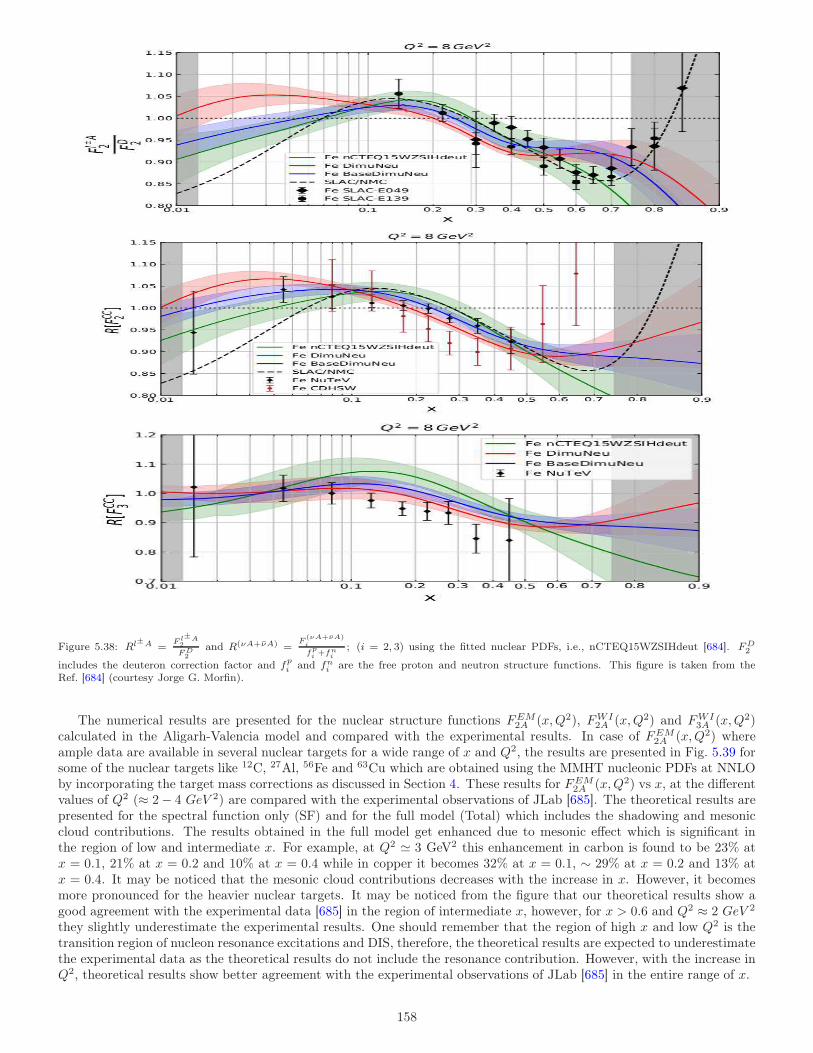
Figure 5.38: Rl±A =F l±A2

FD2

and R(νA+νA) =F

(νA+νA)i

fpi+fn

i

; (i = 2, 3) using the fitted nuclear PDFs, i.e., nCTEQ15WZSIHdeut [684]. FD2

includes the deuteron correction factor and fpi and fn

i are the free proton and neutron structure functions. This figure is taken from theRef. [684] (courtesy Jorge G. Morfin).

The numerical results are presented for the nuclear structure functions FEM2A (x,Q2), FWI

2A (x,Q2) and FWI3A (x,Q2)

calculated in the Aligarh-Valencia model and compared with the experimental results. In case of FEM2A (x,Q2) where

ample data are available in several nuclear targets for a wide range of x and Q2, the results are presented in Fig. 5.39 forsome of the nuclear targets like 12C, 27Al, 56Fe and 63Cu which are obtained using the MMHT nucleonic PDFs at NNLOby incorporating the target mass corrections as discussed in Section 4. These results for FEM

2A (x,Q2) vs x, at the differentvalues of Q2 (≈ 2− 4 GeV 2) are compared with the experimental observations of JLab [685]. The theoretical results arepresented for the spectral function only (SF) and for the full model (Total) which includes the shadowing and mesoniccloud contributions. The results obtained in the full model get enhanced due to mesonic effect which is significant inthe region of low and intermediate x. For example, at Q2 ≃ 3 GeV2 this enhancement in carbon is found to be 23% atx = 0.1, 21% at x = 0.2 and 10% at x = 0.4 while in copper it becomes 32% at x = 0.1, ∼ 29% at x = 0.2 and 13% atx = 0.4. It may be noticed that the mesonic cloud contributions decreases with the increase in x. However, it becomesmore pronounced for the heavier nuclear targets. It may be noticed from the figure that our theoretical results show agood agreement with the experimental data [685] in the region of intermediate x, however, for x > 0.6 and Q2 ≈ 2 GeV 2

they slightly underestimate the experimental results. One should remember that the region of high x and low Q2 is thetransition region of nucleon resonance excitations and DIS, therefore, the theoretical results are expected to underestimatethe experimental data as the theoretical results do not include the resonance contribution. However, with the increase inQ2, theoretical results show better agreement with the experimental observations of JLab [685] in the entire range of x.

158

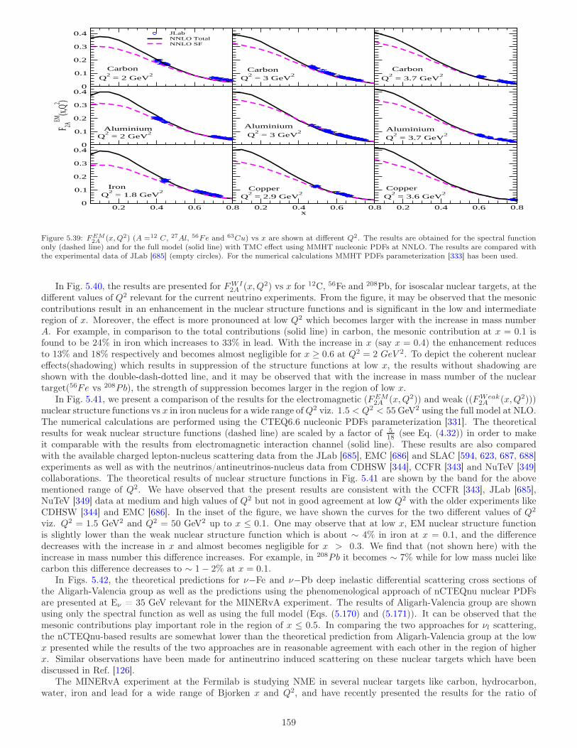
0

0.1

0.2

0.3

0.4 JLabNNLO TotalNNLO SF

0

0.1

0.2

0.3

0.4

F 2A

EM(x,

Q2 )

0.2 0.4 0.6 0.80

0.1

0.2

0.3

0.4

0.2 0.4 0.6 0.8x

0.2 0.4 0.6 0.8

Carbon

Q2 = 2 GeV

2Carbon

Q2 = 3 GeV

2Carbon

Q2 = 3.7 GeV

2

Q2 = 2 GeV

2 Q2 = 3 GeV

2Aluminium Aluminium Aluminium

Q2 = 3.7 GeV

2

IronQ

2 = 1.8 GeV

2Q

2 = 2.9 GeV

2Copper Copper

Q2 = 3.6 GeV

2

Figure 5.39: FEM2A (x,Q2) (A =12 C, 27Al, 56Fe and 63Cu) vs x are shown at different Q2. The results are obtained for the spectral function

only (dashed line) and for the full model (solid line) with TMC effect using MMHT nucleonic PDFs at NNLO. The results are compared withthe experimental data of JLab [685] (empty circles). For the numerical calculations MMHT PDFs parameterization [333] has been used.

In Fig. 5.40, the results are presented for FWI2A (x,Q2) vs x for 12C, 56Fe and 208Pb, for isoscalar nuclear targets, at the

different values of Q2 relevant for the current neutrino experiments. From the figure, it may be observed that the mesoniccontributions result in an enhancement in the nuclear structure functions and is significant in the low and intermediateregion of x. Moreover, the effect is more pronounced at low Q2 which becomes larger with the increase in mass numberA. For example, in comparison to the total contributions (solid line) in carbon, the mesonic contribution at x = 0.1 isfound to be 24% in iron which increases to 33% in lead. With the increase in x (say x = 0.4) the enhancement reducesto 13% and 18% respectively and becomes almost negligible for x ≥ 0.6 at Q2 = 2 GeV 2. To depict the coherent nucleareffects(shadowing) which results in suppression of the structure functions at low x, the results without shadowing areshown with the double-dash-dotted line, and it may be observed that with the increase in mass number of the nucleartarget(56Fe vs 208Pb), the strength of suppression becomes larger in the region of low x.

In Fig. 5.41, we present a comparison of the results for the electromagnetic (FEM2A (x,Q2)) and weak ((FWeak

2A (x,Q2)))nuclear structure functions vs x in iron nucleus for a wide range ofQ2 viz. 1.5 < Q2 < 55 GeV2 using the full model at NLO.The numerical calculations are performed using the CTEQ6.6 nucleonic PDFs parameterization [331]. The theoreticalresults for weak nuclear structure functions (dashed line) are scaled by a factor of 5

18 (see Eq. (4.32)) in order to makeit comparable with the results from electromagnetic interaction channel (solid line). These results are also comparedwith the available charged lepton-nucleus scattering data from the JLab [685], EMC [686] and SLAC [594, 623, 687, 688]experiments as well as with the neutrinos/antineutrinos-nucleus data from CDHSW [344], CCFR [343] and NuTeV [349]collaborations. The theoretical results of nuclear structure functions in Fig. 5.41 are shown by the band for the abovementioned range of Q2. We have observed that the present results are consistent with the CCFR [343], JLab [685],NuTeV [349] data at medium and high values of Q2 but not in good agreement at low Q2 with the older experiments likeCDHSW [344] and EMC [686]. In the inset of the figure, we have shown the curves for the two different values of Q2

viz. Q2 = 1.5 GeV2 and Q2 = 50 GeV2 up to x ≤ 0.1. One may observe that at low x, EM nuclear structure functionis slightly lower than the weak nuclear structure function which is about ∼ 4% in iron at x = 0.1, and the differencedecreases with the increase in x and almost becomes negligible for x > 0.3. We find that (not shown here) with theincrease in mass number this difference increases. For example, in 208Pb it becomes ∼ 7% while for low mass nuclei likecarbon this difference decreases to ∼ 1− 2% at x = 0.1.

In Figs. 5.42, the theoretical predictions for ν−Fe and ν−Pb deep inelastic differential scattering cross sections ofthe Aligarh-Valencia group as well as the predictions using the phenomenological approach of nCTEQnu nuclear PDFsare presented at Eν = 35 GeV relevant for the MINERvA experiment. The results of Aligarh-Valencia group are shownusing only the spectral function as well as using the full model (Eqs. (5.170) and (5.171)). It can be observed that themesonic contributions play important role in the region of x ≤ 0.5. In comparing the two approaches for νl scattering,the nCTEQnu-based results are somewhat lower than the theoretical prediction from Aligarh-Valencia group at the lowx presented while the results of the two approaches are in reasonable agreement with each other in the region of higherx. Similar observations have been made for antineutrino induced scattering on these nuclear targets which have beendiscussed in Ref. [126].

The MINERvA experiment at the Fermilab is studying NME in several nuclear targets like carbon, hydrocarbon,water, iron and lead for a wide range of Bjorken x and Q2, and have recently presented the results for the ratio of

159

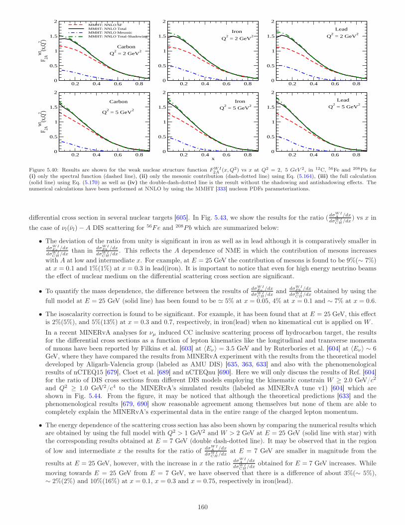
0.2 0.4 0.6 0.80

0.5

1

1.5

2

F 2A

WI (x

,Q2 )

MMHT: NNLO SFMMHT: NNLO TotalMMHT: NNLO MesonicMMHT: NNLO Total-Shadowing

0.2 0.4 0.6 0.80

0.5

1

1.5

2

0.2 0.4 0.6 0.80

0.5

1

1.5

2

0.2 0.4 0.6 0.80

0.5

1

1.5

2

F 2A

WI (x

,Q2 )

0.2 0.4 0.6 0.8x

0

0.5

1

1.5

2

0.2 0.4 0.6 0.80

0.5

1

1.5

2

Carbon

Iron Lead

Q2 = 5 GeV

2

Q2 = 2 GeV

2

Carbon Iron

Q2 = 5 GeV

2 Q2 = 5 GeV

2Lead

Q2 = 2 GeV

2 Q2 = 2 GeV

2

Figure 5.40: Results are shown for the weak nuclear structure function FWI2A (x,Q2) vs x at Q2 = 2, 5 GeV 2, in 12C, 56Fe and 208Pb for

(i) only the spectral function (dashed line), (ii) only the mesonic contribution (dash-dotted line) using Eq. (5.164), (iii) the full calculation(solid line) using Eq. (5.170) as well as (iv) the double-dash-dotted line is the result without the shadowing and antishadowing effects. Thenumerical calculations have been performed at NNLO by using the MMHT [333] nucleon PDFs parameterizations.

differential cross section in several nuclear targets [605]. In Fig. 5.43, we show the results for the ratio (dσWI

A /dx

dσWICH/dx

) vs x in

the case of νl(νl)−A DIS scattering for 56Fe and 208Pb which are summarized below:

• The deviation of the ratio from unity is significant in iron as well as in lead although it is comparatively smaller indσWI

Fe /dx

dσWICH

/dxthan in

dσWIPb /dx

dσWICH

/dx. This reflects the A dependence of NME in which the contribution of mesons increases

with A at low and intermediate x. For example, at E = 25 GeV the contribution of mesons is found to be 9%(∼ 7%)at x = 0.1 and 1%(1%) at x = 0.3 in lead(iron). It is important to notice that even for high energy neutrino beamsthe effect of nuclear medium on the differential scattering cross section are significant.

• To quantify the mass dependence, the difference between the results ofdσWI

Fe /dx

dσWICH/dx

anddσWI

Pb /dx

dσWICH/dx

obtained by using the

full model at E = 25 GeV (solid line) has been found to be ≃ 5% at x = 0.05, 4% at x = 0.1 and ∼ 7% at x = 0.6.

• The isoscalarity correction is found to be significant. For example, it has been found that at E = 25 GeV, this effectis 2%(5%), and 5%(13%) at x = 0.3 and 0.7, respectively, in iron(lead) when no kinematical cut is applied on W .

In a recent MINERvA analyses for νµ induced CC inclusive scattering process off hydrocarbon target, the resultsfor the differential cross sections as a function of lepton kinematics like the longitudinal and transverse momentaof muons have been reported by Filkins et al. [603] at 〈Eν〉 = 3.5 GeV and by Ruterbories et al. [604] at 〈Eν〉 ∼ 6GeV, where they have compared the results from MINERvA experiment with the results from the theoretical modeldeveloped by Aligarh-Valencia group (labeled as AMU DIS) [635, 363, 633] and also with the phenomenologicalresults of nCTEQ15 [679], Cloet et al. [689] and nCTEQnu [690]. Here we will only discuss the results of Ref. [604]for the ratio of DIS cross sections from different DIS models employing the kinematic constrain W ≥ 2.0 GeV/c2

and Q2 ≥ 1.0 GeV2/c4 to the MINERvA’s simulated results (labeled as MINERvA tune v1) [604] which areshown in Fig. 5.44. From the figure, it may be noticed that although the theoretical predictions [633] and thephenomenological results [679, 690] show reasonable agreement among themselves but none of them are able tocompletely explain the MINERvA’s experimental data in the entire range of the charged lepton momentum.

• The energy dependence of the scattering cross section has also been shown by comparing the numerical results whichare obtained by using the full model with Q2 > 1 GeV2 and W > 2 GeV at E = 25 GeV (solid line with star) withthe corresponding results obtained at E = 7 GeV (double dash-dotted line). It may be observed that in the region

of low and intermediate x the results for the ratio ofdσWI

A /dx

dσWICH

/dxat E = 7 GeV are smaller in magnitude from the

results at E = 25 GeV, however, with the increase in x the ratiodσWI

A /dx

dσWICH/dx

obtained for E = 7 GeV increases. While

moving towards E = 25 GeV from E = 7 GeV, we have observed that there is a difference of about 3%(∼ 5%),∼ 2%(2%) and 10%(16%) at x = 0.1, x = 0.3 and x = 0.75, respectively in iron(lead).

160

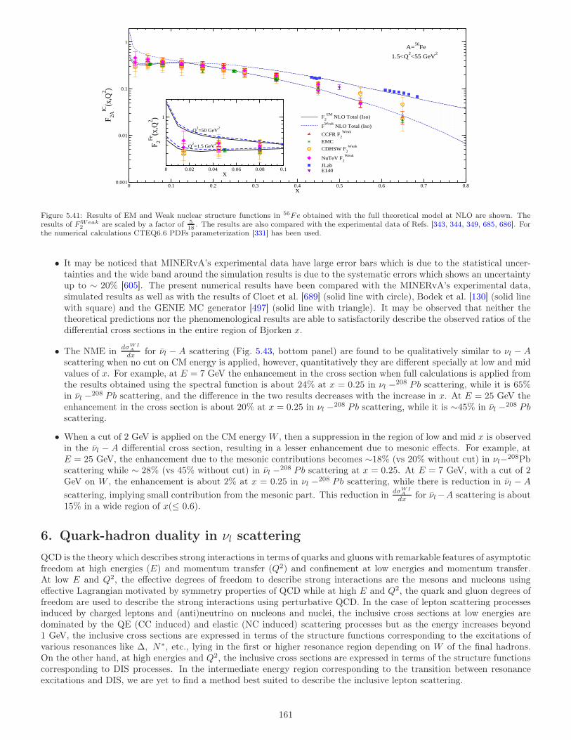
0 0.02 0.04 0.06 0.08 0.1x

1

F 2Fe(x

,Q2 )

0 0.1 0.2 0.3 0.4 0.5 0.6 0.7 0.8x

0.001

0.01

0.1

1

F 2A

IC(x

,Q2 )

F2

EM NLO Total (Iso)

FWeak

NLO Total (Iso)

CCFR F2

Weak

EMC

CDHSW F2

Weak

NuTeV F2

Weak

JLabE140

1.5<Q2<55 GeV

2A=

56Fe

Q2=50 GeV

2

Q2=1.5 GeV

2

Figure 5.41: Results of EM and Weak nuclear structure functions in 56Fe obtained with the full theoretical model at NLO are shown. Theresults of FWeak

2 are scaled by a factor of 518

. The results are also compared with the experimental data of Refs. [343, 344, 349, 685, 686]. Forthe numerical calculations CTEQ6.6 PDFs parameterization [331] has been used.

• It may be noticed that MINERvA’s experimental data have large error bars which is due to the statistical uncer-tainties and the wide band around the simulation results is due to the systematic errors which shows an uncertaintyup to ∼ 20% [605]. The present numerical results have been compared with the MINERvA’s experimental data,simulated results as well as with the results of Cloet et al. [689] (solid line with circle), Bodek et al. [130] (solid linewith square) and the GENIE MC generator [497] (solid line with triangle). It may be observed that neither thetheoretical predictions nor the phenomenological results are able to satisfactorily describe the observed ratios of thedifferential cross sections in the entire region of Bjorken x.

• The NME indσWI

A

dx for νl − A scattering (Fig. 5.43, bottom panel) are found to be qualitatively similar to νl − Ascattering when no cut on CM energy is applied, however, quantitatively they are different specially at low and midvalues of x. For example, at E = 7 GeV the enhancement in the cross section when full calculations is applied fromthe results obtained using the spectral function is about 24% at x = 0.25 in νl −208 Pb scattering, while it is 65%in νl −208 Pb scattering, and the difference in the two results decreases with the increase in x. At E = 25 GeV theenhancement in the cross section is about 20% at x = 0.25 in νl −208 Pb scattering, while it is ∼45% in νl −208 Pbscattering.

• When a cut of 2 GeV is applied on the CM energy W , then a suppression in the region of low and mid x is observedin the νl − A differential cross section, resulting in a lesser enhancement due to mesonic effects. For example, atE = 25 GeV, the enhancement due to the mesonic contributions becomes ∼18% (vs 20% without cut) in νl−208Pbscattering while ∼ 28% (vs 45% without cut) in νl −208 Pb scattering at x = 0.25. At E = 7 GeV, with a cut of 2GeV on W , the enhancement is about 2% at x = 0.25 in νl −208 Pb scattering, while there is reduction in νl − Ascattering, implying small contribution from the mesonic part. This reduction in

dσWIA

dx for νl−A scattering is about15% in a wide region of x(≤ 0.6).

6. Quark-hadron duality in νl scattering

QCD is the theory which describes strong interactions in terms of quarks and gluons with remarkable features of asymptoticfreedom at high energies (E) and momentum transfer (Q2) and confinement at low energies and momentum transfer.At low E and Q2, the effective degrees of freedom to describe strong interactions are the mesons and nucleons usingeffective Lagrangian motivated by symmetry properties of QCD while at high E and Q2, the quark and gluon degrees offreedom are used to describe the strong interactions using perturbative QCD. In the case of lepton scattering processesinduced by charged leptons and (anti)neutrino on nucleons and nuclei, the inclusive cross sections at low energies aredominated by the QE (CC induced) and elastic (NC induced) scattering processes but as the energy increases beyond1 GeV, the inclusive cross sections are expressed in terms of the structure functions corresponding to the excitations ofvarious resonances like ∆, N∗, etc., lying in the first or higher resonance region depending on W of the final hadrons.On the other hand, at high energies and Q2, the inclusive cross sections are expressed in terms of the structure functionscorresponding to DIS processes. In the intermediate energy region corresponding to the transition between resonanceexcitations and DIS, we are yet to find a method best suited to describe the inclusive lepton scattering.

161

0 0.2 0.4 0.6 0.8 10

1

2

3

(1/E

)*(d

2 σ A

WI /

dx d

y) 1

0-38 c

m2 -G

eV-1

NuTeVSF NocutTotal NocutnCTEQnu

0 0.2 0.4 0.6 0.8 10

0.5

1

1.5

0 0.2 0.4 0.6 0.8 10

0.1

0.2

0.3

0.4

0.5

0 0.2 0.4 0.60

1

2

Total Wcut

0 0.1 0.2 0.3 0.4 0.50

0.2

0.4

0 0.1 0.2 0.3 0.4 0.50

0.5

1

1.5

x=0.225x=0.45

x=0.65

νl-56

Fe νl-56

Feν

l-56

FeE=35 GeV

0 0.2 0.4 0.6 0.8 10

0.5

1

1.5

2

2.5

3

(1/E

)*(d

2 σ A

WI /

dx d

y) 1

0-38 c

m2 -G

eV-1

CHORUSSF NocutTotal NocutnCTEQnu

0 0.2 0.4 0.6 0.8 10

0.5

1

1.5

0 0.2 0.4 0.6 0.8 10

0.1

0.2

0.3

0.4

0.5

0 0.2 0.4 0.6 0.80

1

2

Total Wcut

0 0.1 0.2 0.3 0.4 0.50

0.5

1

1.5

0 0.1 0.2 0.3 0.4 0.50

0.10.20.30.40.5

x=0.225 x=0.45 x=0.65

νl-208

Pb νl-208

Pb νl-208

Pb

E=35 GeV

Figure 5.42: Differential cross section vs y for the different values of x for the incomice-20 mm and ν-Pb DIS (bottom row). Theoreticalpredictions are shown with the spectral function only (dashed line) and with the full model (solid line) at NNLO. In the inset the effects of anadditional kinematical cut of W ≥ 2 GeV (solid line with star) for the full theoretical model are shown. The blue dash-dotted line in the toprow is the result from nCTEQnu nPDFs with Q2 ≥ 1.0 GeV 2. Solid circles with error bars are the limited experimental data points of NuTeVat this lower energy.

0 0.1 0.2 0.3 0.4 0.5 0.6 0.7x

0.7

0.8

0.9

1

1.1

1.2

(dσ Fe

WI / d

x) /

(dσCH

WI / d

x)

SimulationBY13GENIECloet et al.MINERvA DataTotal Wcut (E=7 GeV)SF Wcut (E=25 Gev)Total Nocut (E=25 GeV)Total Wcut (E=25 GeV)

Nonisoscalar

νl

0 0.1 0.2 0.3 0.4 0.5 0.6 0.7x

0.7

0.8

0.9

1

1.1

1.2

1.3

(dσ Pb

WI / d

x) /

(dσCH

WI / d

x)

SimulationCloet et al.GENIEBY13MINERvA DataSF Wcut (E=25 GeV)Total Wcut (E=25 GeV)Total Nocut (E=25 GeV)Total Wcut (E=7 GeV)

Nonisoscalar

νl

0 0.1 0.2 0.3 0.4 0.5 0.6 0.7x

0.5

0.75

1

1.25

1.5

(dσFe

WI /dx

) / (d

σ CH

WI /dx

)

Total Wcut (E=7 GeV)SF Wcut (E=25 GeV)Total Wcut (E=25 GeV)Total Nocut (E=25 GeV)

0 0.1 0.2 0.3 0.4 0.5 0.6 0.7x

0.5

0.75

1

1.25

1.5

(dσPb

WI /dx

) / (d

σ CH

WI /dx

)

Total Wcut (E=7 GeV)SF Wcut (E=25 GeV)Total Wcut (E=25 GeV)Total Nocut (E=25 GeV)

Nonisoscalar Nonisoscalarν

lν

l

Figure 5.43:dσWI

A /dx

dσWICH

/dx(A = 56Fe, 208Pb) vs x for incoming neutrino (top panel) and antineutrino (bottom panel) beam of energies E = 7 GeV

and 25 GeV. The numerical results are obtained with the spectral function only (dash-dotted line: E = 25 GeV) as well as with the full model(solid line: E = 25 GeV, solid line with star: E = 25 GeV and double dash-dotted line: E = 7 GeV) at NNLO and are compared with thephenomenological results of Cloet et al. [689], Bodek-Yang [130], GENIE Monte Carlo [497] and with the simulated results [605]. The solidsquares are the experimental points of MINERvA [605]. The results are shown for the nonisoscalar nuclear targets.

162

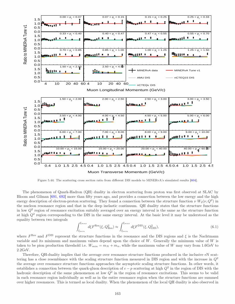
0.00.51.01.5

< 2.50t

1.50 < p

4 10 20 40 60

0.00.51.01.5

< 0.85t

0.70 < p0.00.51.01.5

< 0.40t

0.33 < p0.00.51.01.5

< 0.07t

0.00 < p

< 4.50t

2.50 < p

4 10 20 40 60

< 1.00t

0.85 < p

< 0.47t

0.40 < p

< 0.15t

0.07 < p

< 1.25t

1.00 < p

< 0.55t

0.47 < p

< 0.25t

0.15 < p

MINERvA data MINERvA Tune v1

AMU DIS nCTEQ15 DIS

DISνnCTEQ

< 1.50t

1.25 < p

< 0.70t

0.55 < p

< 0.33t

0.25 < p

Muon Longitudinal Momentum (GeV/c)

Ratio

to M

INER

vA T

une

v1

0.00.51.01.5

< 15.00||

10.00 < p

0.4 1.0 1.5 2.5 4.5

0.00.51.01.5

< 7.00||

6.00 < p0.00.51.01.5

< 4.00||

3.50 < p0.00.51.01.5

< 2.00||

1.50 < p

< 20.00||

15.00 < p

0.4 1.0 1.5 2.5 4.5

< 8.00||

7.00 < p

< 4.50||

4.00 < p

< 2.50||

2.00 < p

< 40.00||

20.00 < p

0.4 1.0 1.5 2.5 4.5

< 9.00||

8.00 < p

< 5.00||

4.50 < p

< 3.00||

2.50 < p

< 60.00||

40.00 < p

0.4 1.0 1.5 2.5 4.5

< 10.00||

9.00 < p

< 6.00||

5.00 < p

< 3.50||

3.00 < p

Muon Transverse Momentum (GeV/c)

Ratio

to M

INER

vA T

une

v1

Figure 5.44: The scattering cross section ratio from different DIS models to MINERvA’s simulated results [604].

The phenomenon of Quark-Hadron (QH) duality in electron scattering from proton was first observed at SLAC byBloom and Gilman [691, 692] more than fifty years ago, and provides a connection between the low energy and the highenergy description of electron-proton scattering. They found a connection between the structure function ν W2(ν,Q

2) inthe nucleon resonance region and that in the deep inelastic continuum. QH duality states that the structure functionsin low Q2 region of resonance excitation suitably averaged over an energy interval is the same as the structure functionat high Q2 region corresponding to the DIS in the same energy interval. At the basic level it may be understood as theequality between two integrals

∫ ξmax

ξmin

dξFRes(ξ,Q2Res) ≈

∫ ξmax

ξmin

dξFDIS(ξ,Q2DIS), (6.1)

where FRes and F

DIS represent the structure functions in the resonance and the DIS regions and ξ is the Nachtmannvariable and its minimum and maximum values depend upon the choice of W . Generally the minimum value of W istaken to be pion production threshold i.e. Wmin = mN +mπ, while the maximum value of W may vary from 1.6GeV to2.2GeV.

Therefore, QH-duality implies that the average over resonance structure functions produced in the inclusive eN scat-tering has a close resemblance with the scaling structure function measured in DIS region and with the increase in Q2

the average over resonance structure functions approaches the asymptotic scaling structure functions. In other words, itestablishes a connection between the quark-gluon description of e− p scattering at high Q2 in the region of DIS with thehadronic description of the same phenomenon at low Q2 in the region of resonance excitations. This seems to be validin each resonance region individually as well as in the entire resonance region when the structure functions are summedover higher resonances. This is termed as local duality. When the phenomenon of the local QH duality is also observed in

163

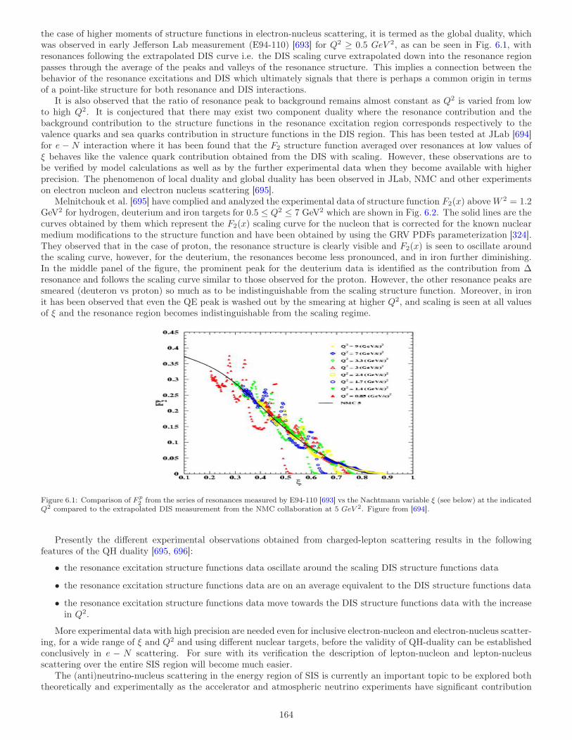
the case of higher moments of structure functions in electron-nucleus scattering, it is termed as the global duality, whichwas observed in early Jefferson Lab measurement (E94-110) [693] for Q2 ≥ 0.5 GeV 2, as can be seen in Fig. 6.1, withresonances following the extrapolated DIS curve i.e. the DIS scaling curve extrapolated down into the resonance regionpasses through the average of the peaks and valleys of the resonance structure. This implies a connection between thebehavior of the resonance excitations and DIS which ultimately signals that there is perhaps a common origin in termsof a point-like structure for both resonance and DIS interactions.

It is also observed that the ratio of resonance peak to background remains almost constant as Q2 is varied from lowto high Q2. It is conjectured that there may exist two component duality where the resonance contribution and thebackground contribution to the structure functions in the resonance excitation region corresponds respectively to thevalence quarks and sea quarks contribution in structure functions in the DIS region. This has been tested at JLab [694]for e − N interaction where it has been found that the F2 structure function averaged over resonances at low values ofξ behaves like the valence quark contribution obtained from the DIS with scaling. However, these observations are tobe verified by model calculations as well as by the further experimental data when they become available with higherprecision. The phenomenon of local duality and global duality has been observed in JLab, NMC and other experimentson electron nucleon and electron nucleus scattering [695].

Melnitchouk et al. [695] have complied and analyzed the experimental data of structure function F2(x) aboveW 2 = 1.2GeV2 for hydrogen, deuterium and iron targets for 0.5 ≤ Q2 ≤ 7 GeV2 which are shown in Fig. 6.2. The solid lines are thecurves obtained by them which represent the F2(x) scaling curve for the nucleon that is corrected for the known nuclearmedium modifications to the structure function and have been obtained by using the GRV PDFs parameterization [324].They observed that in the case of proton, the resonance structure is clearly visible and F2(x) is seen to oscillate aroundthe scaling curve, however, for the deuterium, the resonances become less pronounced, and in iron further diminishing.In the middle panel of the figure, the prominent peak for the deuterium data is identified as the contribution from ∆resonance and follows the scaling curve similar to those observed for the proton. However, the other resonance peaks aresmeared (deuteron vs proton) so much as to be indistinguishable from the scaling structure function. Moreover, in ironit has been observed that even the QE peak is washed out by the smearing at higher Q2, and scaling is seen at all valuesof ξ and the resonance region becomes indistinguishable from the scaling regime.

Figure 6.1: Comparison of F p2 from the series of resonances measured by E94-110 [693] vs the Nachtmann variable ξ (see below) at the indicated

Q2 compared to the extrapolated DIS measurement from the NMC collaboration at 5 GeV 2. Figure from [694].

Presently the different experimental observations obtained from charged-lepton scattering results in the followingfeatures of the QH duality [695, 696]:

• the resonance excitation structure functions data oscillate around the scaling DIS structure functions data

• the resonance excitation structure functions data are on an average equivalent to the DIS structure functions data

• the resonance excitation structure functions data move towards the DIS structure functions data with the increasein Q2.

More experimental data with high precision are needed even for inclusive electron-nucleon and electron-nucleus scatter-ing, for a wide range of ξ and Q2 and using different nuclear targets, before the validity of QH-duality can be establishedconclusively in e − N scattering. For sure with its verification the description of lepton-nucleon and lepton-nucleusscattering over the entire SIS region will become much easier.

The (anti)neutrino-nucleus scattering in the energy region of SIS is currently an important topic to be explored boththeoretically and experimentally as the accelerator and atmospheric neutrino experiments have significant contribution

164

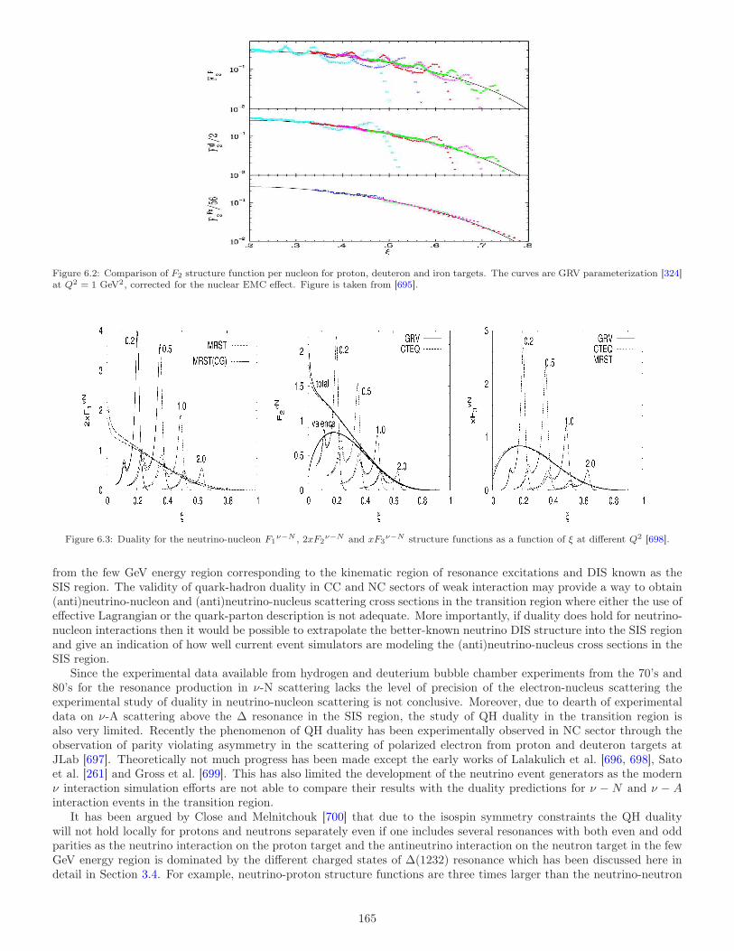
Figure 6.2: Comparison of F2 structure function per nucleon for proton, deuteron and iron targets. The curves are GRV parameterization [324]at Q2 = 1 GeV2, corrected for the nuclear EMC effect. Figure is taken from [695].

Figure 6.3: Duality for the neutrino-nucleon F1ν−N , 2xF2

ν−N and xF3ν−N structure functions as a function of ξ at different Q2 [698].

from the few GeV energy region corresponding to the kinematic region of resonance excitations and DIS known as theSIS region. The validity of quark-hadron duality in CC and NC sectors of weak interaction may provide a way to obtain(anti)neutrino-nucleon and (anti)neutrino-nucleus scattering cross sections in the transition region where either the use ofeffective Lagrangian or the quark-parton description is not adequate. More importantly, if duality does hold for neutrino-nucleon interactions then it would be possible to extrapolate the better-known neutrino DIS structure into the SIS regionand give an indication of how well current event simulators are modeling the (anti)neutrino-nucleus cross sections in theSIS region.

Since the experimental data available from hydrogen and deuterium bubble chamber experiments from the 70’s and80’s for the resonance production in ν-N scattering lacks the level of precision of the electron-nucleus scattering theexperimental study of duality in neutrino-nucleon scattering is not conclusive. Moreover, due to dearth of experimentaldata on ν-A scattering above the ∆ resonance in the SIS region, the study of QH duality in the transition region isalso very limited. Recently the phenomenon of QH duality has been experimentally observed in NC sector through theobservation of parity violating asymmetry in the scattering of polarized electron from proton and deuteron targets atJLab [697]. Theoretically not much progress has been made except the early works of Lalakulich et al. [696, 698], Satoet al. [261] and Gross et al. [699]. This has also limited the development of the neutrino event generators as the modernν interaction simulation efforts are not able to compare their results with the duality predictions for ν − N and ν − Ainteraction events in the transition region.

It has been argued by Close and Melnitchouk [700] that due to the isospin symmetry constraints the QH dualitywill not hold locally for protons and neutrons separately even if one includes several resonances with both even and oddparities as the neutrino interaction on the proton target and the antineutrino interaction on the neutron target in the fewGeV energy region is dominated by the different charged states of ∆(1232) resonance which has been discussed here indetail in Section 3.4. For example, neutrino-proton structure functions are three times larger than the neutrino-neutron

165

structure functions and therefore resonance structure functions are significantly larger than the leading twist functions

i.e. Fνp(reason)i > F

νp(LT)i . This clearly indicates the violation of QH-duality for neutrino interaction on a proton target.

Similarly for a neutrino-neutron scattering besides the contribution from the isospin 32 resonances, there is also significant

contribution from the isospin 12 resonances, but the total contribution from isospin 1

2 resonances is smaller than that from

isospin 32 resonances due to ∆(1232) dominance which results F

νn(reason)i < F

νn(LT)i . Thus QH-duality is also not valid

for ν − n scattering.Therefore, one considers duality for the average of proton and neutron structure functions. This has been studied

by Lalakulich et al. [698] in neutrino-nucleon scattering as well as in neutrino-nucleus interactions [696] and they findthat for an isoscalar nucleon target duality holds, which has been shown here in Fig. 6.3 for the neutrino-nucleon F1

ν−N ,2xF2

ν−N and xF3ν−N structure functions at several values of Q2. It may be observed that for ν −N scattering duality

holds good for F2 and F3 and not so well for F1.Geissen-Ghent collaboration [696] have studied Bloom-Gilman duality, in electron and neutrino scattering on nuclei,

and found that the ratio

I(Q2Res, Q

2DIS) =

∫ ξmax

ξmindξ FRes

j (ξ,Q2Res)

∫ ξmax

ξmindξ FDIS

j (ξ,Q2DIS)

< 1, (6.2)

where Fj represents 2xF1, F2, and xF3, where Res (DIS) represent resonance (DIS) structure functions at same ξ.They [696] have emphasized the importance of including NR as well as resonance contributions while evaluating thenumerator in Eq. (6.2).

To conclude, the study of QH duality needs serious attention especially by the neutrino physics community as asubstantial contribution to the events is expected to come from the transition region for all the next generation plannedaccelerator and atmospheric neutrino experiments.

7. Monte Carlo event generators and some of the recent results from the

accelerator experiments

Monte Carlo event generators are scientific programs/libraries to simulate events for the neutrino interactions withmatter (electrons, nucleons and nuclei). In the neutrino sector, the early event generators were NEUGEN [701], NU-ANCE [306], NUX [702], NEUT [703, 704] and Geneve [705]. These were initially developed by the experimenters tosimulate events for a particular experiment. For example, the earliest version of the NEUGEN event generator was writtenfor the Soudan 2 experiment, in the mid-1980’s, to simulate the neutrino backgrounds in the proton decay searches. Inthe earlier version of NUANCE and NEUGEN, to simulate neutrino interactions with the nuclear targets, Smith andMoniz model was used for the QE scattering from nuclei, Rein and Sehgal model was used for the resonance excitation,and for the DIS, the NME like the shadowing, anti-shadowing, Fermi motion and EMC were not considered. Laterwith the need of more sophisticated and robust event generators, several collaborative projects were started which ledto the amalgamation of theorists, phenomenologists as well as experimenters in the development of the neutrino eventgenerators. The recent Monte Carlo generators widely used in the accelerator and atmospheric neutrino experiments areGENIE [497, 378], NEUT [703, 704], NuWro [499], GiBUU [536], FLUKA [706], etc., which are updated regularly by therespective developers.

There are now provisions of alternative nuclear models for the QE scattering like the Smith and Moniz Fermi gasmodel, LFGM of the Valencia group, Superscaling model of Donnelly group, more sophisticated models to take intoaccount many body nucleon correlation effects like the inclusion of 2p-2h effect using either the formalism of Martini etal. [463, 464, 465, 466] or Nieves et al. [467, 707], and the final state interaction effects, etc.

Most of these modern generators (GENIE, NEUT, NuWro) have common inputs. However, the differences in theirimplementation, the value of the parameters used, and approaches to avoid double counting yield different predictions.For example, in the earlier version of GENIE, the QE scattering is modeled using the relativistic Fermi gas model ofLlewellyn Smith, for the baryon resonance excitations in NC and CC channels Rein and Sehgal model is used in which 16resonances were considered and DIS is calculated using Bodek and Yang prescription. Recent version of GENIE 3 usesdifferent models of NME for the QE neutrino induced processes like LFGM of the Valencia group with 1p-1h and 2p-2hexcitations [467, 707], Superscaling approach (1p−1h+2p−2h) of Donnelly et al. [708], etc., GENIE is widely being usedby experimenters involved in the Fermilab neutrino program like MINERvA, NOvA, MicroBooNE collaborations. TheseMC generators have now become essential in analyzing the neutrino events as they make use of the latest developmentsin nuclear theory to the description of ν −A interaction cross sections.

NEUT was developed initially by the Kamiokande collaborators to simulate atmospheric neutrino events, it is nowbeing used by the Super-Kamiokande as well as the T2K collaborations and is continuously being updated. One among themany revised versions, NEUT version 5.3.2 describes CCQE neutrino-nucleon interactions using the spectral function (SF)approach of Benhar et al. [709] with MA =1.21GeV. The resonant pion production process is described by the Rein-Sehgalmodel [131] with updated nucleon-resonance transition form-factors [710] and MRes

A =0.95GeV. For the 2p-2h interactions,

166

they have used the microscopic model developed by Nieves et al. [467]. DIS is modeled using GRV98 PDFs [324] withthe corrections by Bodek and Yang [711]. The final state interactions describing the transport of the hadrons produced inthe elementary neutrino interaction through the nucleus, are simulated using a semi-classical intranuclear cascade model.

GiBUU [712] has been developed by Mosel and his collaborators at Giessen, and uses local Thomas-Fermi gas in amean field potential for the QE scattering, for the resonances it uses Mainz Unitary Isobar Model (MAID) analysis ofelectron-nucleon pion production as input for the vector part of both the resonant and NR amplitudes. It is a transportmodel where FSI is implemented by solving Giessen Boltzmann-Uehling-Uhlenbeck (GiBUU) equation. It encompassesa unified framework for hadron, lepton and neutrino interactions with nuclei from a few hundreds of MeV to a few tensof GeV. In recent years, tuned generators like MINERvA tune [713], MicroBooNE tune [714, 715], etc. have been used,where modifications are made in the GENIE or other versions of the generators. For example, it was found by theMINERvA collaboration [713], that the model of Nieves et al. [467], underestimates the 2p-2h strength in the dip regionand therefore they increased the flux-folded strength by a significant amount. For a general discussion, see Ref. [716].

Recently the T2K collaboration [717] plotted the ratio of the double differential cross section per nucleon for νµ inducedCC reaction for oxygen to carbon nuclear targets i.e. RO

C(which has been shown in Fig. 7.1 for the two muon angle bins),

and compared their data with the simulated results from the MC generators like NEUT 5.4.1 LFG, GENIE v3- SuSAv2,NuWro SF, GiBUU, NEUT 5.4.0 SF, GENIE v3 LFG, NuWro LFG and RMF (1p-1h) + SuSAv2 (2p-2h). They have alsopresented the results for the integrated cross sections per nucleon and compared them with the MC predictions [717].

ArgoNeuT collaboration [718] has reported the CC νµ(νµ) induced 1π+(π−) differential cross sections on 40Ar andcompared their results with the MC generators, which are presented in Fig. 7.2. The data for the pion angular distributionand the muon angular distribution obtained by the ArgoNeuT collaboration has been shown, where the comparisons withthe different MCs like GENIE v2_12_2, NuWro 17.01.1, GiBUU and NEUT5.3.7 have also been made [718].

To highlight the difference among the predictions of the various MCs as well as their comparison with the data,in Fig. 7.3, we present an analyses of MINERvA collaboration where they have shown absolute normalized ratios ofdata, and the comparison with the GENIE 2.8.4, NuWro, and GiBUU to MnvGENIEv1 for muon transverse (pT ) andlongitudinal (pL) momenta. It may be observed from Fig. 7.3 that the transverse momentum projection shows tensionamong all models and data in the 0.55 < pT < 1.5 GeV range. While in the case of longitudinal momentum, all modelsunderpredict the cross section.

In Fig. 7.4, we show the recent results of the MicroBooNE collaboration [714], for the total cross section divided by

the bin-center neutrino energy vs neutrino energy i.e.σ(Eνµ )

〈Eνµ〉 vs Eνµ . These results are compared with the MicroBooNE

MC [715], predictions from GENIE v3.0.6 [497, 378], NuWro 19.02.01 [719], NEUT 5.4.0.1 [704], and GiBUU 2019.08 [712].

It may be observed from the above results that there is agreement among the different MC generators with the datanevertheless more work is needed to understand medium effects in the nuclear targets. It needs more collaborative efforts.

8. Summary and outlook

The physics of neutrino interactions with matter has many aspects both in theory and experiment. This is becausethe neutrinos play very significant role in various areas of physics i.e. astrophysics, cosmology, nuclear physics, particlephysics and geophysics. The neutrino physics originated with the attempts to understand the nuclear β decays whichled to the discovery of weak interactions and its role in astrophysical processes of energy generation in stars, synthesis ofelements, supernova explosions, and formation of neutron stars and white dwarfs, etc. With the discovery of new particlesand their weak decays, the neutrino physics became an important component of particle physics both theoretically andexperimentally. The advent of high energy particle accelerators which produced unstable mesons like pions and kaonsleading to the neutrino beams of νµ(νµ) and νe(νe) as their decay products, started the era of νl(νl) scattering fromthe nucleons and nuclei in various energy regions starting from MeV to GeV which was earlier restricted to the verylow energy region of (anti)neutrinos in the region of a few tens of MeV corresponding to the reactor antineutrinos. Theprocesses of (anti)neutrino-nucleon scattering being a weak process has small cross section and therefore requires intense(anti)neutrino beams and large volume target-detectors to enhance the (anti)neutrino induced production of chargedleptons, mesons and photon events to make them statistically significant for physical interpretations. The requirementof large volume target-detectors necessitated the use of medium or heavy nuclear material as targets to perform the(anti)neutrino scattering. This led to various neutrino-nucleus experiments being done at CERN, ANL, BNL, Fermilab,and SKAT using high energy neutrino beams. The confirmation of the phenomenon of neutrino flavor oscillations withthe solar neutrinos and reactor antineutrinos in the low energy region and with the accelerator and atmospheric neutrinosin the intermediate and high energy regions has started great interest in studying the (anti)neutrino-nucleus scatteringin the entire energy region of (anti)neutrino spectrum. Moreover, the study of these processes in the very low energyregion is of immense interest in various astrophysical processes, while in the very high energy region, they are relevantfor studying the origin of cosmic rays.

In view of this, we have presented a review of the (anti)neutrino reactions with nucleons and nuclei in this work.

167

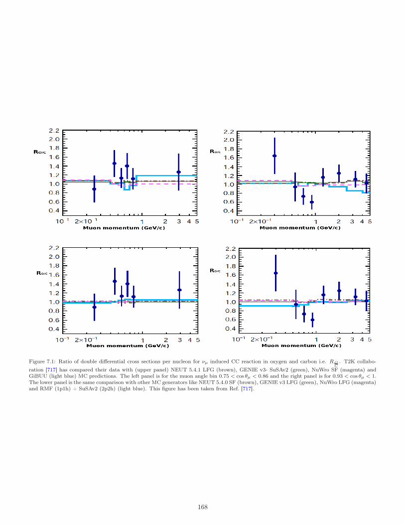
Figure 7.1: Ratio of double differential cross sections per nucleon for νµ induced CC reaction in oxygen and carbon i.e. ROC

. T2K collabo-

ration [717] has compared their data with (upper panel) NEUT 5.4.1 LFG (brown), GENIE v3- SuSAv2 (green), NuWro SF (magenta) andGiBUU (light blue) MC predictions. The left panel is for the muon angle bin 0.75 < cos θµ < 0.86 and the right panel is for 0.93 < cos θµ < 1.The lower panel is the same comparison with other MC generators like NEUT 5.4.0 SF (brown), GENIE v3 LFG (green), NuWro LFG (magenta)and RMF (1p1h) + SuSAv2 (2p2h) (light blue). This figure has been taken from Ref. [717].

168

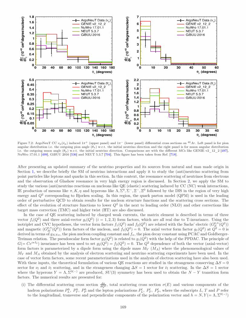
Figure 7.2: ArgoNeuT CC νµ(νµ) induced 1π+ (upper panel) and 1π− (lower panel) differential cross sections on 40Ar. Left panel is for pionangular distribution i.e. the outgoing pion angle (θπ) w.r.t. the initial neutrino direction and the right panel is for muon angular distributioni.e. the outgoing muon angle (θµ) w.r.t. the initial neutrino direction. Comparisons are with the different MCs like GENIE v2_12_2 [497],NuWro 17.01.1 [499], GiBUU 2016 [536] and NEUT 5.3.7 [704]. This figure has been taken from Ref. [718].

After presenting an updated summary of the neutrino properties and its sources from natural and man made origin inSection 1, we describe briefly the SM of neutrino interactions and apply it to study the (anti)neutrino scattering frompoint particles like leptons and quarks in this section. In this context, the resonance scattering of neutrinos from electronsand the observation of Glashow resonance in very high energy region is discussed. In Section 2, we apply the SM tostudy the various (anti)neutrino reactions on nucleons like QE (elastic) scattering induced by CC (NC) weak interactions,IE production of mesons like π,K, η and hyperons like Λ,Σ0,Σ−,Ξ−,Ξ0 followed by the DIS in the region of very highenergy and Q2 corresponding to Bjorken scaling. In this region, the quark parton model (QPM) is used in the leadingorder of perturbative QCD to obtain results for the nucleon structure functions and the scattering cross sections. Theeffect of the evolution of structure functions to lower Q2 in the next to leading order (NLO) and other corrections liketarget mass correction (TMC) and higher twist (HT) are also discussed.

In the case of QE scattering induced by charged weak currents, the matrix element is described in terms of threevector fi(Q

2) and three axial-vector gi(Q2) (i = 1, 2, 3) form factors, which are all real due to T-invariance. Using the

isotriplet and CVC hypotheses, the vector form factors f1(Q2) and f2(Q

2) are related with the Sachs’ electric (Gp,nE (Q2))

and magnetic (Gp,nM (Q2)) form factors of the nucleon, and f3(Q

2) = 0. The axial vector form factor g1(Q2) at Q2 = 0 is

derived in terms of gNNπ, the pion nucleon coupling constant and fπ, the pion decay constant using PCAC and Goldberger-Treiman relation. The pseudoscalar form factor g3(Q

2) is related to g1(Q2) with the help of the PPDAC. The principle of

G(= CeiπI2 ) invariance has been used to set g2(Q2) = f3(Q

2) = 0. The Q2 dependence of both the vector (axial-vector)form factors is parameterized by a dipole form using the dipole mass MV (MA) where the phenomenological values ofMV and MA obtained by the analysis of electron scattering and neutrino scattering experiments have been used. In thecase of vector form factors, some recent parameterizations used in the analysis of electron scattering have also been used.With these inputs, the theoretical formulation of various QE reactions are studied in the strangeness conserving ∆S = 0sector for νl and νl scattering, and in the strangeness changing ∆S = 1 sector for νl scattering. In the ∆S = 1 sectorwhere the hyperons Y = Λ,Σ0(−) are produced, SU(3) symmetry has been used to obtain the N − Y transition formfactors. The numerical results are presented for:

(i) The differential scattering cross section dσdQ2 , total scattering cross section σ(E) and various components of the

hadron polarizations P hL , P

hT , P

hP and the lepton polarizations P l

L, PlT , P

lP , where the subscripts L, T and P refer

to the longitudinal, transverse and perpendicular components of the polarization vector and h = N, Y (= Λ,Σ0(−))

169

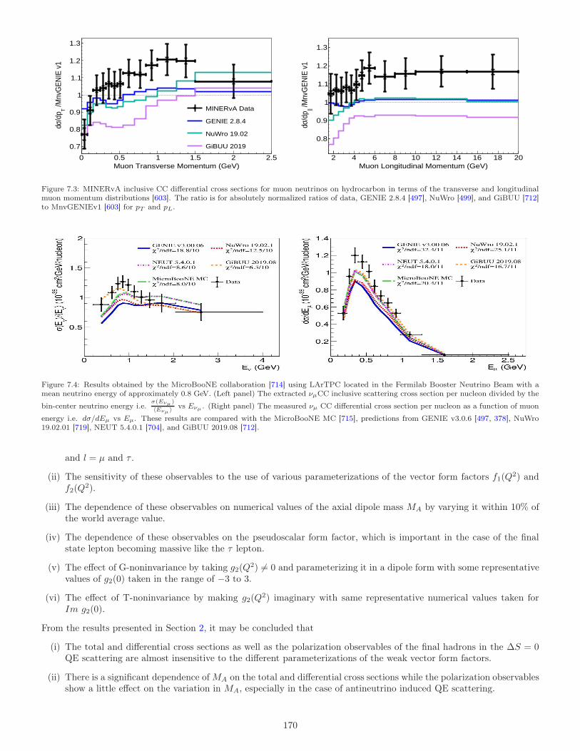
Muon Transverse Momentum (GeV)0 0.5 1 1.5 2 2.5

/Mnv

GE

NIE

v1

T/d

pσd

0.7

0.8

0.9

1

1.1

1.2

1.3

MINERvA Data

GENIE 2.8.4

NuWro 19.02

GiBUU 2019

Muon Longitudinal Momentum (GeV)2 4 6 8 10 12 14 16 18 20

/Mnv

GE

NIE

v1

||/d

pσd

0.8

0.9

1

1.1

1.2

1.3

Figure 7.3: MINERvA inclusive CC differential cross sections for muon neutrinos on hydrocarbon in terms of the transverse and longitudinalmuon momentum distributions [603]. The ratio is for absolutely normalized ratios of data, GENIE 2.8.4 [497], NuWro [499], and GiBUU [712]to MnvGENIEv1 [603] for pT and pL.

Figure 7.4: Results obtained by the MicroBooNE collaboration [714] using LArTPC located in the Fermilab Booster Neutrino Beam with amean neutrino energy of approximately 0.8 GeV. (Left panel) The extracted νµCC inclusive scattering cross section per nucleon divided by the

bin-center neutrino energy i.e.σ(Eνµ)

〈Eνµ 〉 vs Eνµ . (Right panel) The measured νµ CC differential cross section per nucleon as a function of muon

energy i.e. dσ/dEµ vs Eµ. These results are compared with the MicroBooNE MC [715], predictions from GENIE v3.0.6 [497, 378], NuWro19.02.01 [719], NEUT 5.4.0.1 [704], and GiBUU 2019.08 [712].

and l = µ and τ .

(ii) The sensitivity of these observables to the use of various parameterizations of the vector form factors f1(Q2) and

f2(Q2).

(iii) The dependence of these observables on numerical values of the axial dipole mass MA by varying it within 10% ofthe world average value.

(iv) The dependence of these observables on the pseudoscalar form factor, which is important in the case of the finalstate lepton becoming massive like the τ lepton.

(v) The effect of G-noninvariance by taking g2(Q2) 6= 0 and parameterizing it in a dipole form with some representative

values of g2(0) taken in the range of −3 to 3.

(vi) The effect of T-noninvariance by making g2(Q2) imaginary with same representative numerical values taken for

Im g2(0).

From the results presented in Section 2, it may be concluded that

(i) The total and differential cross sections as well as the polarization observables of the final hadrons in the ∆S = 0QE scattering are almost insensitive to the different parameterizations of the weak vector form factors.

(ii) There is a significant dependence of MA on the total and differential cross sections while the polarization observablesshow a little effect on the variation in MA, especially in the case of antineutrino induced QE scattering.

170

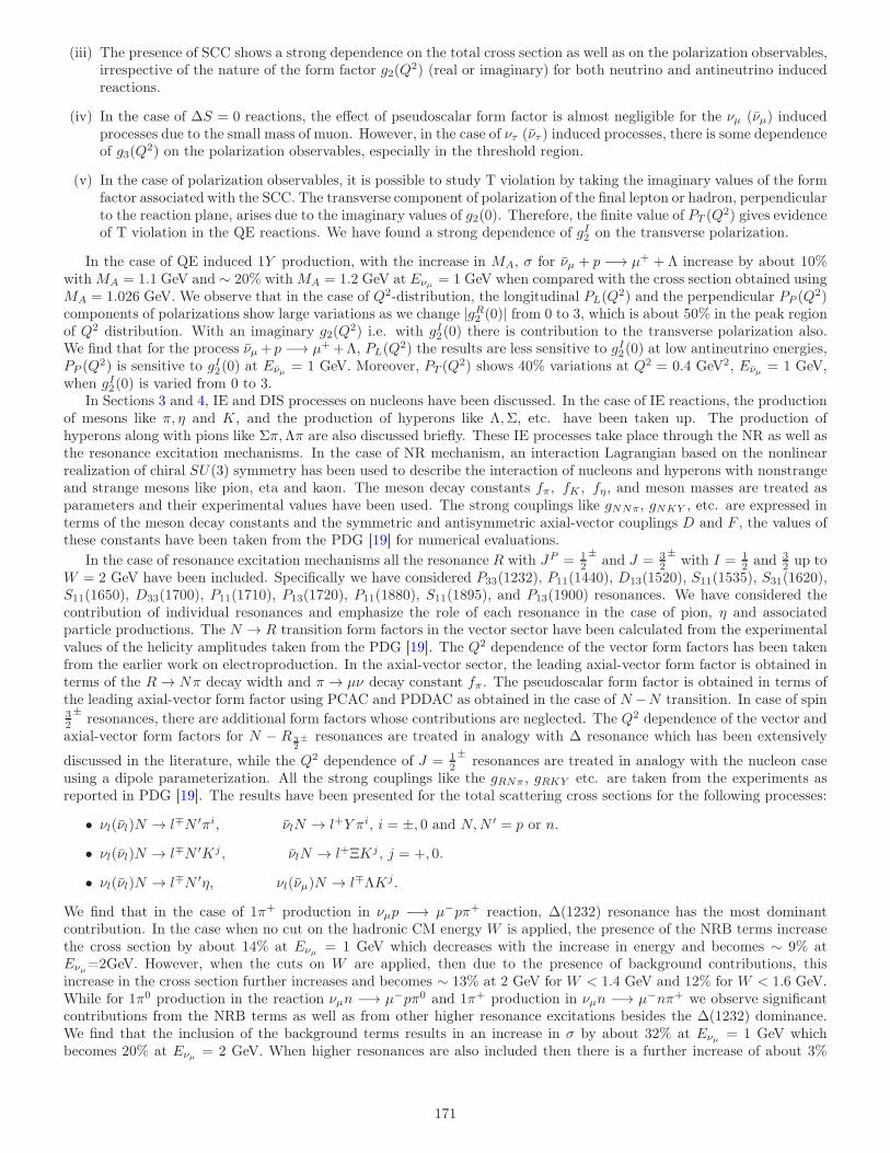
(iii) The presence of SCC shows a strong dependence on the total cross section as well as on the polarization observables,irrespective of the nature of the form factor g2(Q

2) (real or imaginary) for both neutrino and antineutrino inducedreactions.

(iv) In the case of ∆S = 0 reactions, the effect of pseudoscalar form factor is almost negligible for the νµ (νµ) inducedprocesses due to the small mass of muon. However, in the case of ντ (ντ ) induced processes, there is some dependenceof g3(Q

2) on the polarization observables, especially in the threshold region.

(v) In the case of polarization observables, it is possible to study T violation by taking the imaginary values of the formfactor associated with the SCC. The transverse component of polarization of the final lepton or hadron, perpendicularto the reaction plane, arises due to the imaginary values of g2(0). Therefore, the finite value of PT (Q

2) gives evidenceof T violation in the QE reactions. We have found a strong dependence of gI2 on the transverse polarization.

In the case of QE induced 1Y production, with the increase in MA, σ for νµ + p −→ µ+ + Λ increase by about 10%with MA = 1.1 GeV and ∼ 20% with MA = 1.2 GeV at Eνµ = 1 GeV when compared with the cross section obtained usingMA = 1.026 GeV. We observe that in the case of Q2-distribution, the longitudinal PL(Q

2) and the perpendicular PP (Q2)

components of polarizations show large variations as we change |gR2 (0)| from 0 to 3, which is about 50% in the peak regionof Q2 distribution. With an imaginary g2(Q

2) i.e. with gI2(0) there is contribution to the transverse polarization also.We find that for the process νµ+p −→ µ++Λ, PL(Q

2) the results are less sensitive to gI2(0) at low antineutrino energies,PP (Q

2) is sensitive to gI2(0) at Eνµ = 1 GeV. Moreover, PT (Q2) shows 40% variations at Q2 = 0.4 GeV2, Eνµ = 1 GeV,

when gI2(0) is varied from 0 to 3.In Sections 3 and 4, IE and DIS processes on nucleons have been discussed. In the case of IE reactions, the production

of mesons like π, η and K, and the production of hyperons like Λ,Σ, etc. have been taken up. The production ofhyperons along with pions like Σπ,Λπ are also discussed briefly. These IE processes take place through the NR as well asthe resonance excitation mechanisms. In the case of NR mechanism, an interaction Lagrangian based on the nonlinearrealization of chiral SU(3) symmetry has been used to describe the interaction of nucleons and hyperons with nonstrangeand strange mesons like pion, eta and kaon. The meson decay constants fπ, fK , fη, and meson masses are treated asparameters and their experimental values have been used. The strong couplings like gNNπ, gNKY , etc. are expressed interms of the meson decay constants and the symmetric and antisymmetric axial-vector couplings D and F , the values ofthese constants have been taken from the PDG [19] for numerical evaluations.

In the case of resonance excitation mechanisms all the resonance R with JP = 12

±and J = 3

2

±with I = 1

2 and 32 up to

W = 2 GeV have been included. Specifically we have considered P33(1232), P11(1440), D13(1520), S11(1535), S31(1620),S11(1650), D33(1700), P11(1710), P13(1720), P11(1880), S11(1895), and P13(1900) resonances. We have considered thecontribution of individual resonances and emphasize the role of each resonance in the case of pion, η and associatedparticle productions. The N → R transition form factors in the vector sector have been calculated from the experimentalvalues of the helicity amplitudes taken from the PDG [19]. The Q2 dependence of the vector form factors has been takenfrom the earlier work on electroproduction. In the axial-vector sector, the leading axial-vector form factor is obtained interms of the R→ Nπ decay width and π → µν decay constant fπ. The pseudoscalar form factor is obtained in terms ofthe leading axial-vector form factor using PCAC and PDDAC as obtained in the case of N −N transition. In case of spin32

±resonances, there are additional form factors whose contributions are neglected. The Q2 dependence of the vector and

axial-vector form factors for N − R 32± resonances are treated in analogy with ∆ resonance which has been extensively

discussed in the literature, while the Q2 dependence of J = 12

±resonances are treated in analogy with the nucleon case

using a dipole parameterization. All the strong couplings like the gRNπ, gRKY etc. are taken from the experiments asreported in PDG [19]. The results have been presented for the total scattering cross sections for the following processes:

• νl(νl)N → l∓N ′πi, νlN → l+Y πi, i = ±, 0 and N,N ′ = p or n.

• νl(νl)N → l∓N ′Kj , νlN → l+ΞKj , j = +, 0.

• νl(νl)N → l∓N ′η, νl(νµ)N → l∓ΛKj.

We find that in the case of 1π+ production in νµp −→ µ−pπ+ reaction, ∆(1232) resonance has the most dominantcontribution. In the case when no cut on the hadronic CM energy W is applied, the presence of the NRB terms increasethe cross section by about 14% at Eνµ = 1 GeV which decreases with the increase in energy and becomes ∼ 9% atEνµ=2GeV. However, when the cuts on W are applied, then due to the presence of background contributions, thisincrease in the cross section further increases and becomes ∼ 13% at 2 GeV for W < 1.4 GeV and 12% for W < 1.6 GeV.While for 1π0 production in the reaction νµn −→ µ−pπ0 and 1π+ production in νµn −→ µ−nπ+ we observe significantcontributions from the NRB terms as well as from other higher resonance excitations besides the ∆(1232) dominance.We find that the inclusion of the background terms results in an increase in σ by about 32% at Eνµ = 1 GeV whichbecomes 20% at Eνµ = 2 GeV. When higher resonances are also included then there is a further increase of about 3%

171

at Eνµ = 1 GeV and 40% at Eνµ = 2 GeV. Similar observations have been made for the antineutrino induced processesleading to one pion production.

For η production in νµ+n −→ µ−+η+p and νµ+p −→ µ++η+n reactions, we find that S11(1535) resonance excitationgives the most dominant contribution and the contribution from the NRB terms and from the S11(1650) and P11(1710)resonance excitations are almost negligible. For the single kaon production in νµp −→ µ−K+p and νµn −→ µ−K0preactions, the contact term has the dominant contribution to the total scattering cross section. Similar observation ismade for the antineutrino induced process where an antikaon is produced.

For the associated particle production in the reaction νµ + n −→ µ− + Λ + K+ and νµ + p −→ µ+ + Λ + K0, thebackground terms give the largest contribution and the contributions from the resonances like S11(1650), P11(1710) andP13(1720) considered in this work are small. In the case of neutrino induced KΛ production, P11(1710) has the largestcontribution among the resonances. While in the case of antineutrino induced associated particle production processes, adestructive interference between the background and the resonance terms occurs and the results obtained with backgroundterms only are almost two times the results of full model in the entire energy range. Among the resonances, the mostdominant contribution is from P13(1720) followed by P11(1710) and S11(1650) in the low energy region (Eνµ < 1.5 GeV).We would like to emphasize that the results of single hyperon production cross sections are larger at low antineutrinoenergies in the region of 1.2 GeV and are comparable even at Eνµ = 2 GeV with the cross sections for the associatedparticle production of hyperons obtained in the present model.

In the case of DIS, the cross sections are calculated in the leading order of the perturbative QCD using the QPMin terms of the nucleon structure functions FN

i (x,Q2); i = 1 − 5, using the Callan-Gross relation between F2(x,Q2) and

F1(x,Q2), and Albright-Jarlskog relation between F5(x,Q

2) and F2(x,Q2). The evaluation of the structure functions

Fi(x,Q2) (i = 1, 2, 3, 5) at NLO and NNLO has been obtained using DGLAP equations for which results have been

quoted. The corrections to the nucleon structure functions due to TMC and HT effects have been described qualitativelyso that they can be applied to lower Q2 connecting to SIS or the transition region. We find these corrections to besubstantial in some regions of x and Q2.

Finally in Section 5, we study the NME in the QE, IE and DIS. In the case of QE scattering, NME are described inthe low energy as well as in the intermediate energy regions. In the low energy region relevant to the solar, reactor andaccelerator neutrinos (for (anti)neutrinos obtained from pions and kaons decaying at rest), the exclusive reactions havebeen studied in some nuclei like 12C and 56Fe, using the method based on multipole expansion. The NME are included byusing the nuclear wave functions calculated with realistic nucleon-nucleon potentials which include the effect of nucleoncorrelations and pairing, etc. and reproduce the binding energy and other static properties of the nuclei.

In the region of intermediate and higher energies the method based on LFGM has been used in which the longrange correlations are included in a RPA approach to augment the results obtained by calculating the cross sections andangular as well as the energy distributions of the final state leptons based on the 1p-1h excitation. Further modificationsof the cross sections and energy/angular distributions due to the 2p-2h and MEC have been discussed and the results arecompared with the experimental results obtained by the MiniBooNE, T2K, MINERvA, etc. collaborations.

The effects due to Fermi motion, Pauli blocking, binding energy, etc. reduces the cross section by ∼ 30(42)% atEν = 0.3 GeV which becomes 20(30)% at Eν = 0.6 GeV, compared to the free nucleon case. When RPA correlationeffects are included a further reduction of ∼ 55(56)% at Eν = 0.3 GeV and 35(45)% at Eν = 0.6 GeV is obtained.This reduction further gets enhanced when A is increased in the case of heavier nuclei like 40Ar, 56Fe and 208Pb. Due tothreshold effect, the reduction is larger for νµ and νµ induced CCQE processes at lower energies, which has been discussedquantitatively in Section 5.4.3.

For the single hyperon production in νµ induced CCQE process, the effects of Fermi motion and Pauli blocking arefound to be negligible, while the effect of FSI is substantial, for example, the enhancement in the Λ production crosssection is 22–25% in 12C and 16O for Eνµ = 0.6− 1 GeV, which increases to 34–38% in 40Ar and 52–62% in 208Pb. Whilethe decrease in Σ− production cross section is about 40–46% in 12C and 16O for Eνµ = 0.6 − 1 GeV, which becomes50–56% in 40Ar and 68–70% in 208Pb. The FSI effect also results in the production of Σ+, which is forbidden in thefree nucleon case due to the ∆S = ∆Q rule. These hyperons decay to pions in the nucleus and these pions contributesignificantly to the total 1π production for Eνµ < 1.2GeV, which is generally dominated by the ∆ resonance.

In the case of IE processes, NME are discussed only in the case of pion production which are dominated by the ∆-excitation. The nuclear medium modifications of the properties of ∆, specially in their mass and decay width have beenincluded in calculating the ∆ excitation and its decays. After pions are produced in the nuclear medium, the final stateinteraction of pions with nucleons in the medium is included in a Monte Carlo approach in which the pions go throughthe process of elastic scattering, charge exchange scattering and absorption as they travel through the medium. We findthat NME and FSI effects together results in a net reduction of about 40% to the total pion production for neutrinos of1 GeV energy range.

In the case of DIS, NME are included by calculating the nucleon spectral function S(~p,E) for the initial nucleon ina relativistic field theoretical approach to describe the momentum distribution of the nucleon which includes the effectof nuclear binding, Fermi motion and nucleon-nucleon correlations specially the long range correlation. The nucleonstructure functions FN

i (x,Q2) (i = 1− 5) are then convoluted with the spectral function to include NME and the nuclear

172

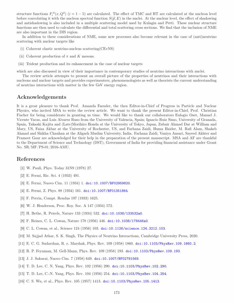
structure functions FAi (x,Q2) (i = 1 − 5) are calculated. The effect of TMC and HT are calculated at the nucleon level

before convoluting it with the nucleon spectral function S(~p,E) in the nuclei. At the nuclear level, the effect of shadowingand antishadowing is also included in a multiple scattering model used by Kulagin and Petti. These nuclear structurefunctions are then used to calculate the differential and total scattering cross sections. We find that the inclusion of NMEare also important in the DIS region.

In addition to these considerations of NME, some new processes also become relevant in the case of (anti)neutrinoscattering with nuclear targets like

(i) Coherent elastic neutrino-nucleus scattering(CEvNS)

(ii) Coherent production of π and K mesons.

(iii) Trident production and its enhancement in the case of nuclear targets

which are also discussed in view of their importance in contemporary studies of neutrino interactions with nuclei.The review article attempts to present an overall picture of the properties of neutrinos and their interactions with

nucleons and nuclear targets and provides experimenters, phenomenologists as well as theorists the current understandingof neutrino interactions with matter in the few GeV energy region.

Acknowledgements

It is a great pleasure to thank Prof. Amanda Faessler, the then Editor-in-Chief of Progress in Particle and NuclearPhysics, who invited MSA to write the review article. We want to thank the present Editor-in-Chief, Prof. ChristianFischer for being considerate in granting us time. We would like to thank our collaborators Eulogio Oset, Manuel J.Vicente Vacas, and Luis Alvarez Ruso from the University of Valencia, Spain; Ignacio Ruiz Simo, University of Granada,Spain, Takaaki Kajita and (Late)Morihiro Honda at the University of Tokyo, Japan, Zubair Ahmad Dar at William andMary, US, Faiza Akbar at the University of Rochester, US, and Farhana Zaidi, Huma Haider, M. Rafi Alam, ShakebAhmad and Shikha Chauhan at the Aligarh Muslim University, India. Farhana Zaidi, Vaniya Ansari, Sayeed Akhter andPrameet Gaur are acknowledged for their help in the preparation of the present manuscript. MSA and AF are thankfulto the Department of Science and Technology (DST), Government of India for providing financial assistance under GrantNo. SR/MF/PS-01/2016-AMU.

References

[1] W. Pauli, Phys. Today 31N9 (1978) 27.

[2] E. Fermi, Ric. Sci. 4 (1933) 491.

[3] E. Fermi, Nuovo Cim. 11 (1934) 1. doi:10.1007/BF02959820.

[4] E. Fermi, Z. Phys. 88 (1934) 161. doi:10.1007/BF01351864.

[5] F. Perrin, Compt. Rendus 197 (1933) 1625.

[6] W. J. Henderson, Proc. Roy. Soc. A 147 (1934) 572.

[7] H. Bethe, R. Peierls, Nature 133 (1934) 532. doi:10.1038/133532a0.

[8] F. Reines, C. L. Cowan, Nature 178 (1956) 446. doi:10.1038/178446a0.

[9] C. L. Cowan, et al., Science 124 (1956) 103. doi:10.1126/science.124.3212.103.

[10] M. Sajjad Athar, S. K. Singh, The Physics of Neutrino Interactions, Cambridge University Press, 2020.

[11] E. C. G. Sudarshan, R. e. Marshak, Phys. Rev. 109 (1958) 1860. doi:10.1103/PhysRev.109.1860.2.

[12] R. P. Feynman, M. Gell-Mann, Phys. Rev. 109 (1958) 193. doi:10.1103/PhysRev.109.193.

[13] J. J. Sakurai, Nuovo Cim. 7 (1958) 649. doi:10.1007/BF02781569.

[14] T. D. Lee, C. N. Yang, Phys. Rev. 102 (1956) 290. doi:10.1103/PhysRev.102.290.

[15] T. D. Lee, C.-N. Yang, Phys. Rev. 104 (1956) 254. doi:10.1103/PhysRev.104.254.

[16] C. S. Wu, et al., Phys. Rev. 105 (1957) 1413. doi:10.1103/PhysRev.105.1413.

173

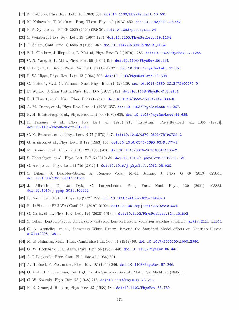
[17] N. Cabibbo, Phys. Rev. Lett. 10 (1963) 531. doi:10.1103/PhysRevLett.10.531.

[18] M. Kobayashi, T. Maskawa, Prog. Theor. Phys. 49 (1973) 652. doi:10.1143/PTP.49.652.

[19] P. A. Zyla, et al., PTEP 2020 (2020) 083C01. doi:10.1093/ptep/ptaa104.

[20] S. Weinberg, Phys. Rev. Lett. 19 (1967) 1264. doi:10.1103/PhysRevLett.19.1264.

[21] A. Salam, Conf. Proc. C 680519 (1968) 367. doi:10.1142/9789812795915_0034.

[22] S. L. Glashow, J. Iliopoulos, L. Maiani, Phys. Rev. D 2 (1970) 1285. doi:10.1103/PhysRevD.2.1285.

[23] C.-N. Yang, R. L. Mills, Phys. Rev. 96 (1954) 191. doi:10.1103/PhysRev.96.191.

[24] F. Englert, R. Brout, Phys. Rev. Lett. 13 (1964) 321. doi:10.1103/PhysRevLett.13.321.

[25] P. W. Higgs, Phys. Rev. Lett. 13 (1964) 508. doi:10.1103/PhysRevLett.13.508.

[26] G. ’t Hooft, M. J. G. Veltman, Nucl. Phys. B 44 (1972) 189. doi:10.1016/0550-3213(72)90279-9.

[27] B. W. Lee, J. Zinn-Justin, Phys. Rev. D 5 (1972) 3121. doi:10.1103/PhysRevD.5.3121.

[28] F. J. Hasert, et al., Nucl. Phys. B 73 (1974) 1. doi:10.1016/0550-3213(74)90038-8.

[29] A. M. Cnops, et al., Phys. Rev. Lett. 41 (1978) 357. doi:10.1103/PhysRevLett.41.357.

[30] R. H. Heisterberg, et al., Phys. Rev. Lett. 44 (1980) 635. doi:10.1103/PhysRevLett.44.635.

[31] H. Faissner, et al., Phys. Rev. Lett. 41 (1978) 213, [Erratum: Phys.Rev.Lett. 41, 1083 (1978)].doi:10.1103/PhysRevLett.41.213.

[32] C. Y. Prescott, et al., Phys. Lett. B 77 (1978) 347. doi:10.1016/0370-2693(78)90722-0.

[33] G. Arnison, et al., Phys. Lett. B 122 (1983) 103. doi:10.1016/0370-2693(83)91177-2.

[34] M. Banner, et al., Phys. Lett. B 122 (1983) 476. doi:10.1016/0370-2693(83)91605-2.

[35] S. Chatrchyan, et al., Phys. Lett. B 716 (2012) 30. doi:10.1016/j.physletb.2012.08.021.

[36] G. Aad, et al., Phys. Lett. B 716 (2012) 1. doi:10.1016/j.physletb.2012.08.020.

[37] S. Bifani, S. Descotes-Genon, A. Romero Vidal, M.-H. Schune, J. Phys. G 46 (2019) 023001.doi:10.1088/1361-6471/aaf5de.

[38] J. Albrecht, D. van Dyk, C. Langenbruch, Prog. Part. Nucl. Phys. 120 (2021) 103885.doi:10.1016/j.ppnp.2021.103885.

[39] R. Aaij, et al., Nature Phys. 18 (2022) 277. doi:10.1038/s41567-021-01478-8.

[40] P. de Simone, EPJ Web Conf. 234 (2020) 01004. doi:10.1051/epjconf/202023401004.

[41] G. Caria, et al., Phys. Rev. Lett. 124 (2020) 161803. doi:10.1103/PhysRevLett.124.161803.

[42] S. Celani, Lepton Flavour Universality tests and Lepton Flavour Violation searches at LHCb. arXiv:2111.11105.

[43] C. A. Argüelles, et al., Snowmass White Paper: Beyond the Standard Model effects on Neutrino Flavor.arXiv:2203.10811.

[44] M. E. Nahmias, Math. Proc. Cambridge Phil. Soc. 31 (1935) 99. doi:10.1017/S0305004100012986.

[45] G. W. Rodeback, J. S. Allen, Phys. Rev. 86 (1952) 446. doi:10.1103/PhysRev.86.446.

[46] A. I. Leipunski, Proe. Cam. Phil. Soe 32 (1936) 301.

[47] A. H. Snell, F. Pleasonton, Phys. Rev. 97 (1955) 246. doi:10.1103/PhysRev.97.246.

[48] O. K.-H. J. C. Jaeobsen, Det. Kgl. Danske Viedensk. Selskab. Mat . Fys. Medd. 23 (1945) 1.

[49] C. W. Sherwin, Phys. Rev. 73 (1948) 216. doi:10.1103/PhysRev.73.216.

[50] H. R. Crane, J. Halpern, Phys. Rev. 53 (1938) 789. doi:10.1103/PhysRev.53.789.

174

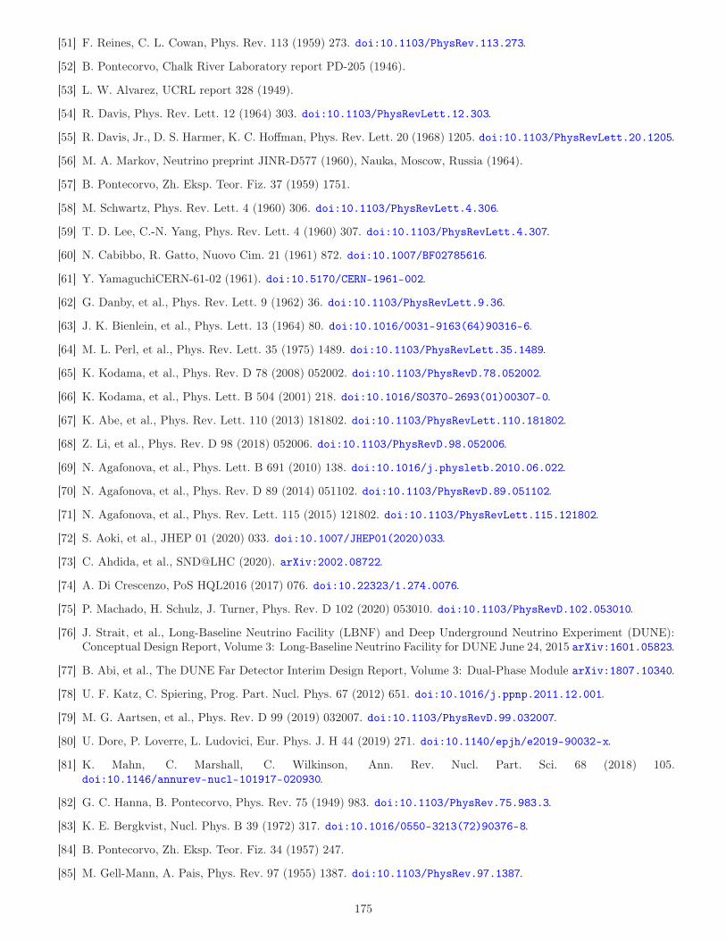
[51] F. Reines, C. L. Cowan, Phys. Rev. 113 (1959) 273. doi:10.1103/PhysRev.113.273.

[52] B. Pontecorvo, Chalk River Laboratory report PD-205 (1946).

[53] L. W. Alvarez, UCRL report 328 (1949).

[54] R. Davis, Phys. Rev. Lett. 12 (1964) 303. doi:10.1103/PhysRevLett.12.303.

[55] R. Davis, Jr., D. S. Harmer, K. C. Hoffman, Phys. Rev. Lett. 20 (1968) 1205. doi:10.1103/PhysRevLett.20.1205.

[56] M. A. Markov, Neutrino preprint JINR-D577 (1960), Nauka, Moscow, Russia (1964).

[57] B. Pontecorvo, Zh. Eksp. Teor. Fiz. 37 (1959) 1751.

[58] M. Schwartz, Phys. Rev. Lett. 4 (1960) 306. doi:10.1103/PhysRevLett.4.306.

[59] T. D. Lee, C.-N. Yang, Phys. Rev. Lett. 4 (1960) 307. doi:10.1103/PhysRevLett.4.307.

[60] N. Cabibbo, R. Gatto, Nuovo Cim. 21 (1961) 872. doi:10.1007/BF02785616.

[61] Y. YamaguchiCERN-61-02 (1961). doi:10.5170/CERN-1961-002.

[62] G. Danby, et al., Phys. Rev. Lett. 9 (1962) 36. doi:10.1103/PhysRevLett.9.36.

[63] J. K. Bienlein, et al., Phys. Lett. 13 (1964) 80. doi:10.1016/0031-9163(64)90316-6.

[64] M. L. Perl, et al., Phys. Rev. Lett. 35 (1975) 1489. doi:10.1103/PhysRevLett.35.1489.

[65] K. Kodama, et al., Phys. Rev. D 78 (2008) 052002. doi:10.1103/PhysRevD.78.052002.

[66] K. Kodama, et al., Phys. Lett. B 504 (2001) 218. doi:10.1016/S0370-2693(01)00307-0.

[67] K. Abe, et al., Phys. Rev. Lett. 110 (2013) 181802. doi:10.1103/PhysRevLett.110.181802.

[68] Z. Li, et al., Phys. Rev. D 98 (2018) 052006. doi:10.1103/PhysRevD.98.052006.

[69] N. Agafonova, et al., Phys. Lett. B 691 (2010) 138. doi:10.1016/j.physletb.2010.06.022.

[70] N. Agafonova, et al., Phys. Rev. D 89 (2014) 051102. doi:10.1103/PhysRevD.89.051102.

[71] N. Agafonova, et al., Phys. Rev. Lett. 115 (2015) 121802. doi:10.1103/PhysRevLett.115.121802.

[72] S. Aoki, et al., JHEP 01 (2020) 033. doi:10.1007/JHEP01(2020)033.

[73] C. Ahdida, et al., SND@LHC (2020). arXiv:2002.08722.

[74] A. Di Crescenzo, PoS HQL2016 (2017) 076. doi:10.22323/1.274.0076.

[75] P. Machado, H. Schulz, J. Turner, Phys. Rev. D 102 (2020) 053010. doi:10.1103/PhysRevD.102.053010.

[76] J. Strait, et al., Long-Baseline Neutrino Facility (LBNF) and Deep Underground Neutrino Experiment (DUNE):Conceptual Design Report, Volume 3: Long-Baseline Neutrino Facility for DUNE June 24, 2015 arXiv:1601.05823.

[77] B. Abi, et al., The DUNE Far Detector Interim Design Report, Volume 3: Dual-Phase Module arXiv:1807.10340.

[78] U. F. Katz, C. Spiering, Prog. Part. Nucl. Phys. 67 (2012) 651. doi:10.1016/j.ppnp.2011.12.001.

[79] M. G. Aartsen, et al., Phys. Rev. D 99 (2019) 032007. doi:10.1103/PhysRevD.99.032007.

[80] U. Dore, P. Loverre, L. Ludovici, Eur. Phys. J. H 44 (2019) 271. doi:10.1140/epjh/e2019-90032-x.

[81] K. Mahn, C. Marshall, C. Wilkinson, Ann. Rev. Nucl. Part. Sci. 68 (2018) 105.doi:10.1146/annurev-nucl-101917-020930.

[82] G. C. Hanna, B. Pontecorvo, Phys. Rev. 75 (1949) 983. doi:10.1103/PhysRev.75.983.3.

[83] K. E. Bergkvist, Nucl. Phys. B 39 (1972) 317. doi:10.1016/0550-3213(72)90376-8.

[84] B. Pontecorvo, Zh. Eksp. Teor. Fiz. 34 (1957) 247.

[85] M. Gell-Mann, A. Pais, Phys. Rev. 97 (1955) 1387. doi:10.1103/PhysRev.97.1387.

175

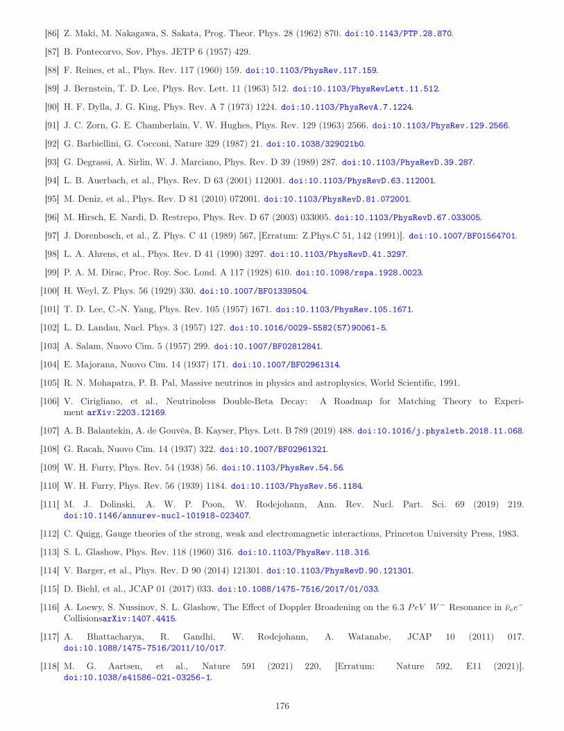
[86] Z. Maki, M. Nakagawa, S. Sakata, Prog. Theor. Phys. 28 (1962) 870. doi:10.1143/PTP.28.870.

[87] B. Pontecorvo, Sov. Phys. JETP 6 (1957) 429.

[88] F. Reines, et al., Phys. Rev. 117 (1960) 159. doi:10.1103/PhysRev.117.159.

[89] J. Bernstein, T. D. Lee, Phys. Rev. Lett. 11 (1963) 512. doi:10.1103/PhysRevLett.11.512.

[90] H. F. Dylla, J. G. King, Phys. Rev. A 7 (1973) 1224. doi:10.1103/PhysRevA.7.1224.

[91] J. C. Zorn, G. E. Chamberlain, V. W. Hughes, Phys. Rev. 129 (1963) 2566. doi:10.1103/PhysRev.129.2566.

[92] G. Barbiellini, G. Cocconi, Nature 329 (1987) 21. doi:10.1038/329021b0.

[93] G. Degrassi, A. Sirlin, W. J. Marciano, Phys. Rev. D 39 (1989) 287. doi:10.1103/PhysRevD.39.287.

[94] L. B. Auerbach, et al., Phys. Rev. D 63 (2001) 112001. doi:10.1103/PhysRevD.63.112001.

[95] M. Deniz, et al., Phys. Rev. D 81 (2010) 072001. doi:10.1103/PhysRevD.81.072001.

[96] M. Hirsch, E. Nardi, D. Restrepo, Phys. Rev. D 67 (2003) 033005. doi:10.1103/PhysRevD.67.033005.

[97] J. Dorenbosch, et al., Z. Phys. C 41 (1989) 567, [Erratum: Z.Phys.C 51, 142 (1991)]. doi:10.1007/BF01564701.

[98] L. A. Ahrens, et al., Phys. Rev. D 41 (1990) 3297. doi:10.1103/PhysRevD.41.3297.

[99] P. A. M. Dirac, Proc. Roy. Soc. Lond. A 117 (1928) 610. doi:10.1098/rspa.1928.0023.

[100] H. Weyl, Z. Phys. 56 (1929) 330. doi:10.1007/BF01339504.

[101] T. D. Lee, C.-N. Yang, Phys. Rev. 105 (1957) 1671. doi:10.1103/PhysRev.105.1671.

[102] L. D. Landau, Nucl. Phys. 3 (1957) 127. doi:10.1016/0029-5582(57)90061-5.

[103] A. Salam, Nuovo Cim. 5 (1957) 299. doi:10.1007/BF02812841.

[104] E. Majorana, Nuovo Cim. 14 (1937) 171. doi:10.1007/BF02961314.

[105] R. N. Mohapatra, P. B. Pal, Massive neutrinos in physics and astrophysics, World Scientific, 1991.

[106] V. Cirigliano, et al., Neutrinoless Double-Beta Decay: A Roadmap for Matching Theory to Experi-ment arXiv:2203.12169.

[107] A. B. Balantekin, A. de Gouvêa, B. Kayser, Phys. Lett. B 789 (2019) 488. doi:10.1016/j.physletb.2018.11.068.

[108] G. Racah, Nuovo Cim. 14 (1937) 322. doi:10.1007/BF02961321.

[109] W. H. Furry, Phys. Rev. 54 (1938) 56. doi:10.1103/PhysRev.54.56.

[110] W. H. Furry, Phys. Rev. 56 (1939) 1184. doi:10.1103/PhysRev.56.1184.

[111] M. J. Dolinski, A. W. P. Poon, W. Rodejohann, Ann. Rev. Nucl. Part. Sci. 69 (2019) 219.doi:10.1146/annurev-nucl-101918-023407.

[112] C. Quigg, Gauge theories of the strong, weak and electromagnetic interactions, Princeton University Press, 1983.

[113] S. L. Glashow, Phys. Rev. 118 (1960) 316. doi:10.1103/PhysRev.118.316.

[114] V. Barger, et al., Phys. Rev. D 90 (2014) 121301. doi:10.1103/PhysRevD.90.121301.

[115] D. Biehl, et al., JCAP 01 (2017) 033. doi:10.1088/1475-7516/2017/01/033.

[116] A. Loewy, S. Nussinov, S. L. Glashow, The Effect of Doppler Broadening on the 6.3 PeV W− Resonance in νee−

CollisionsarXiv:1407.4415.

[117] A. Bhattacharya, R. Gandhi, W. Rodejohann, A. Watanabe, JCAP 10 (2011) 017.doi:10.1088/1475-7516/2011/10/017.

[118] M. G. Aartsen, et al., Nature 591 (2021) 220, [Erratum: Nature 592, E11 (2021)].doi:10.1038/s41586-021-03256-1.

176

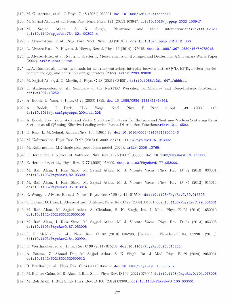
[119] M. G. Aartsen, et al., J. Phys. G 48 (2021) 060501. doi:10.1088/1361-6471/abbd48.

[120] M. Sajjad Athar, et al., Prog. Part. Nucl. Phys. 124 (2022) 103947. doi:10.1016/j.ppnp.2022.103947.

[121] M. Sajjad Athar, S. K. Singh, Neutrinos and their interactionsarXiv:2111.12328,doi:10.1140/epjs/s11734-021-00302-x.

[122] L. Alvarez-Ruso, et al., Prog. Part. Nucl. Phys. 100 (2018) 1. doi:10.1016/j.ppnp.2018.01.006.

[123] L. Alvarez-Ruso, Y. Hayato, J. Nieves, New J. Phys. 16 (2014) 075015. doi:10.1088/1367-2630/16/7/075015.

[124] L. Alvarez-Ruso, et al., Neutrino Scattering Measurements on Hydrogen and Deuterium: A Snowmass White Paper(2022). arXiv:2203.11298.

[125] L. A. Ruso, et al., Theoretical tools for neutrino scattering: interplay between lattice QCD, EFTs, nuclear physics,phenomenology, and neutrino event generators (2022). arXiv:2203.09030.

[126] M. Sajjad Athar, J. G. Morfín, J. Phys. G 48 (2021) 034001. doi:10.1088/1361-6471/abbb11.

[127] C. Andreopoulos, et al., Summary of the NuSTEC Workshop on Shallow- and Deep-Inelastic Scattering.arXiv:1907.13252.

[128] A. Bodek, U. Yang, J. Phys. G 29 (2003) 1899. doi:10.1088/0954-3899/29/8/369.

[129] A. Bodek, I. Park, U.-k. Yang, Nucl. Phys. B Proc. Suppl. 139 (2005) 113.doi:10.1016/j.nuclphysbps.2004.11.208.

[130] A. Bodek, U.-k. Yang, Axial and Vector Structure Functions for Electron- and Neutrino- Nucleon Scattering CrossSections at all Q2 using Effective Leading order Parton Distribution FunctionsarXiv:1011.6592.

[131] D. Rein, L. M. Sehgal, Annals Phys. 133 (1981) 79. doi:10.1016/0003-4916(81)90242-6.

[132] M. Kabirnezhad, Phys. Rev. D 97 (2018) 013002. doi:10.1103/PhysRevD.97.013002.

[133] M. Kabirnezhad, MK single pion production model (2020). arXiv:2006.13765.

[134] E. Hernandez, J. Nieves, M. Valverde, Phys. Rev. D 76 (2007) 033005. doi:10.1103/PhysRevD.76.033005.

[135] E. Hernandez, et al., Phys. Rev. D 77 (2008) 053009. doi:10.1103/PhysRevD.77.053009.

[136] M. Rafi Alam, I. Ruiz Simo, M. Sajjad Athar, M. J. Vicente Vacas, Phys. Rev. D 82 (2010) 033001.doi:10.1103/PhysRevD.82.033001.

[137] M. Rafi Alam, I. Ruiz Simo, M. Sajjad Athar, M. J. Vicente Vacas, Phys. Rev. D 85 (2012) 013014.doi:10.1103/PhysRevD.85.013014.

[138] E. Wang, L. Alvarez-Ruso, J. Nieves, Phys. Rev. C 89 (2014) 015503. doi:10.1103/PhysRevC.89.015503.

[139] T. Leitner, O. Buss, L. Alvarez-Ruso, U. Mosel, Phys. Rev. C 79 (2009) 034601. doi:10.1103/PhysRevC.79.034601.

[140] M. Rafi Alam, M. Sajjad Athar, S. Chauhan, S. K. Singh, Int. J. Mod. Phys. E 25 (2016) 1650010.doi:10.1142/S0218301316500105.

[141] M. Rafi Alam, I. Ruiz Simo, M. Sajjad Athar, M. J. Vicente Vacas, Phys. Rev. D 87 (2013) 053008.doi:10.1103/PhysRevD.87.053008.

[142] E. F. McNicoll, et al., Phys. Rev. C 82 (2010) 035208, [Erratum: Phys.Rev.C 84, 029901 (2011)].doi:10.1103/PhysRevC.84.029901.

[143] D. Werthmüller, et al., Phys. Rev. C 90 (2014) 015205. doi:10.1103/PhysRevC.90.015205.

[144] A. Fatima, Z. Ahmad Dar, M. Sajjad Athar, S. K. Singh, Int. J. Mod. Phys. E 29 (2020) 2050051.doi:10.1142/S0218301320500512.

[145] R. Bradford, et al., Phys. Rev. C 73 (2006) 035202. doi:10.1103/PhysRevC.73.035202.

[146] M. Benitez Galan, M. R. Alam, I. Ruiz Simo, Phys. Rev. D 104 (2021) 073005. doi:10.1103/PhysRevD.104.073005.

[147] M. Rafi Alam, I. Ruiz Simo, Phys. Rev. D 100 (2019) 033001. doi:10.1103/PhysRevD.100.033001.

177

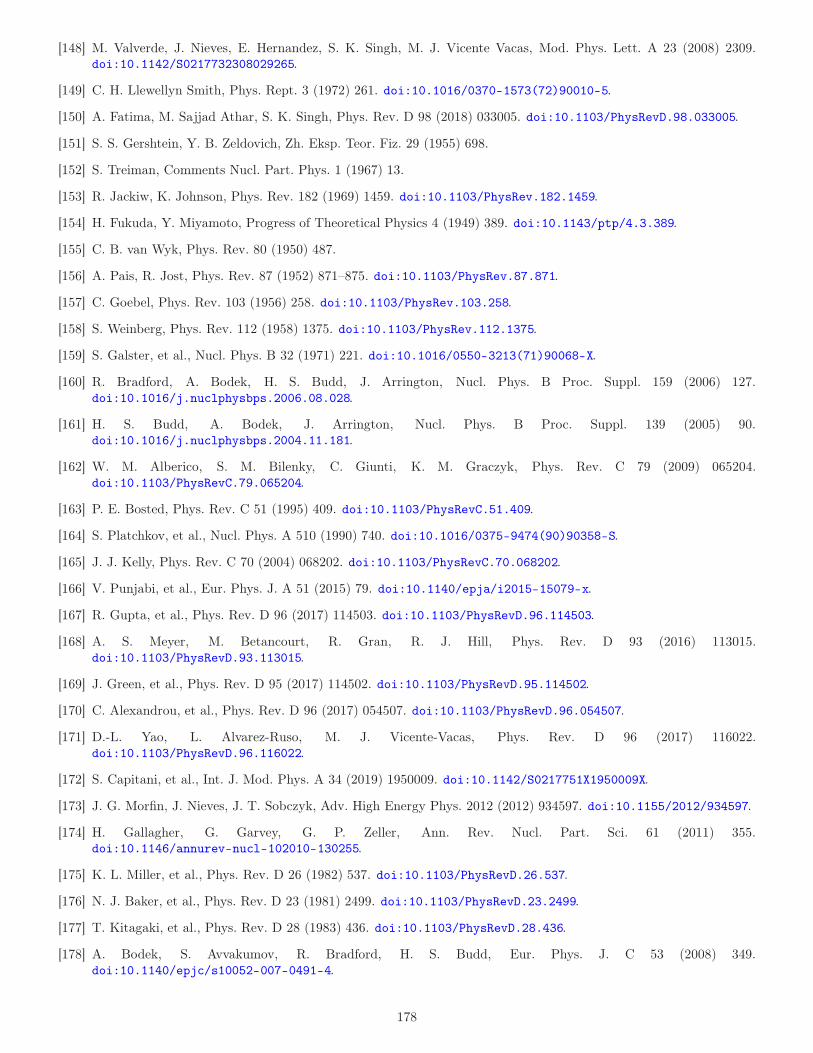
[148] M. Valverde, J. Nieves, E. Hernandez, S. K. Singh, M. J. Vicente Vacas, Mod. Phys. Lett. A 23 (2008) 2309.doi:10.1142/S0217732308029265.

[149] C. H. Llewellyn Smith, Phys. Rept. 3 (1972) 261. doi:10.1016/0370-1573(72)90010-5.

[150] A. Fatima, M. Sajjad Athar, S. K. Singh, Phys. Rev. D 98 (2018) 033005. doi:10.1103/PhysRevD.98.033005.

[151] S. S. Gershtein, Y. B. Zeldovich, Zh. Eksp. Teor. Fiz. 29 (1955) 698.

[152] S. Treiman, Comments Nucl. Part. Phys. 1 (1967) 13.

[153] R. Jackiw, K. Johnson, Phys. Rev. 182 (1969) 1459. doi:10.1103/PhysRev.182.1459.

[154] H. Fukuda, Y. Miyamoto, Progress of Theoretical Physics 4 (1949) 389. doi:10.1143/ptp/4.3.389.

[155] C. B. van Wyk, Phys. Rev. 80 (1950) 487.

[156] A. Pais, R. Jost, Phys. Rev. 87 (1952) 871–875. doi:10.1103/PhysRev.87.871.

[157] C. Goebel, Phys. Rev. 103 (1956) 258. doi:10.1103/PhysRev.103.258.

[158] S. Weinberg, Phys. Rev. 112 (1958) 1375. doi:10.1103/PhysRev.112.1375.

[159] S. Galster, et al., Nucl. Phys. B 32 (1971) 221. doi:10.1016/0550-3213(71)90068-X.

[160] R. Bradford, A. Bodek, H. S. Budd, J. Arrington, Nucl. Phys. B Proc. Suppl. 159 (2006) 127.doi:10.1016/j.nuclphysbps.2006.08.028.

[161] H. S. Budd, A. Bodek, J. Arrington, Nucl. Phys. B Proc. Suppl. 139 (2005) 90.doi:10.1016/j.nuclphysbps.2004.11.181.

[162] W. M. Alberico, S. M. Bilenky, C. Giunti, K. M. Graczyk, Phys. Rev. C 79 (2009) 065204.doi:10.1103/PhysRevC.79.065204.

[163] P. E. Bosted, Phys. Rev. C 51 (1995) 409. doi:10.1103/PhysRevC.51.409.

[164] S. Platchkov, et al., Nucl. Phys. A 510 (1990) 740. doi:10.1016/0375-9474(90)90358-S.

[165] J. J. Kelly, Phys. Rev. C 70 (2004) 068202. doi:10.1103/PhysRevC.70.068202.

[166] V. Punjabi, et al., Eur. Phys. J. A 51 (2015) 79. doi:10.1140/epja/i2015-15079-x.

[167] R. Gupta, et al., Phys. Rev. D 96 (2017) 114503. doi:10.1103/PhysRevD.96.114503.

[168] A. S. Meyer, M. Betancourt, R. Gran, R. J. Hill, Phys. Rev. D 93 (2016) 113015.doi:10.1103/PhysRevD.93.113015.

[169] J. Green, et al., Phys. Rev. D 95 (2017) 114502. doi:10.1103/PhysRevD.95.114502.

[170] C. Alexandrou, et al., Phys. Rev. D 96 (2017) 054507. doi:10.1103/PhysRevD.96.054507.

[171] D.-L. Yao, L. Alvarez-Ruso, M. J. Vicente-Vacas, Phys. Rev. D 96 (2017) 116022.doi:10.1103/PhysRevD.96.116022.

[172] S. Capitani, et al., Int. J. Mod. Phys. A 34 (2019) 1950009. doi:10.1142/S0217751X1950009X.

[173] J. G. Morfin, J. Nieves, J. T. Sobczyk, Adv. High Energy Phys. 2012 (2012) 934597. doi:10.1155/2012/934597.

[174] H. Gallagher, G. Garvey, G. P. Zeller, Ann. Rev. Nucl. Part. Sci. 61 (2011) 355.doi:10.1146/annurev-nucl-102010-130255.

[175] K. L. Miller, et al., Phys. Rev. D 26 (1982) 537. doi:10.1103/PhysRevD.26.537.

[176] N. J. Baker, et al., Phys. Rev. D 23 (1981) 2499. doi:10.1103/PhysRevD.23.2499.

[177] T. Kitagaki, et al., Phys. Rev. D 28 (1983) 436. doi:10.1103/PhysRevD.28.436.

[178] A. Bodek, S. Avvakumov, R. Bradford, H. S. Budd, Eur. Phys. J. C 53 (2008) 349.doi:10.1140/epjc/s10052-007-0491-4.

178

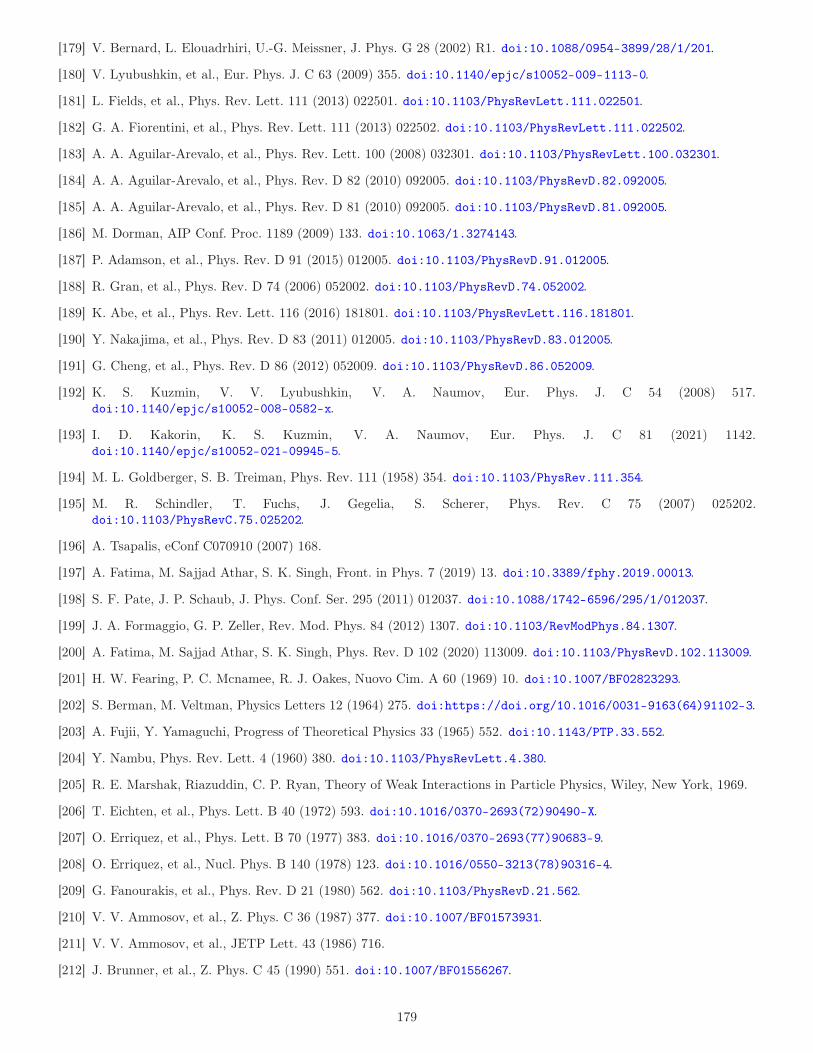
[179] V. Bernard, L. Elouadrhiri, U.-G. Meissner, J. Phys. G 28 (2002) R1. doi:10.1088/0954-3899/28/1/201.

[180] V. Lyubushkin, et al., Eur. Phys. J. C 63 (2009) 355. doi:10.1140/epjc/s10052-009-1113-0.

[181] L. Fields, et al., Phys. Rev. Lett. 111 (2013) 022501. doi:10.1103/PhysRevLett.111.022501.

[182] G. A. Fiorentini, et al., Phys. Rev. Lett. 111 (2013) 022502. doi:10.1103/PhysRevLett.111.022502.

[183] A. A. Aguilar-Arevalo, et al., Phys. Rev. Lett. 100 (2008) 032301. doi:10.1103/PhysRevLett.100.032301.

[184] A. A. Aguilar-Arevalo, et al., Phys. Rev. D 82 (2010) 092005. doi:10.1103/PhysRevD.82.092005.

[185] A. A. Aguilar-Arevalo, et al., Phys. Rev. D 81 (2010) 092005. doi:10.1103/PhysRevD.81.092005.

[186] M. Dorman, AIP Conf. Proc. 1189 (2009) 133. doi:10.1063/1.3274143.

[187] P. Adamson, et al., Phys. Rev. D 91 (2015) 012005. doi:10.1103/PhysRevD.91.012005.

[188] R. Gran, et al., Phys. Rev. D 74 (2006) 052002. doi:10.1103/PhysRevD.74.052002.

[189] K. Abe, et al., Phys. Rev. Lett. 116 (2016) 181801. doi:10.1103/PhysRevLett.116.181801.

[190] Y. Nakajima, et al., Phys. Rev. D 83 (2011) 012005. doi:10.1103/PhysRevD.83.012005.

[191] G. Cheng, et al., Phys. Rev. D 86 (2012) 052009. doi:10.1103/PhysRevD.86.052009.

[192] K. S. Kuzmin, V. V. Lyubushkin, V. A. Naumov, Eur. Phys. J. C 54 (2008) 517.doi:10.1140/epjc/s10052-008-0582-x.

[193] I. D. Kakorin, K. S. Kuzmin, V. A. Naumov, Eur. Phys. J. C 81 (2021) 1142.doi:10.1140/epjc/s10052-021-09945-5.

[194] M. L. Goldberger, S. B. Treiman, Phys. Rev. 111 (1958) 354. doi:10.1103/PhysRev.111.354.

[195] M. R. Schindler, T. Fuchs, J. Gegelia, S. Scherer, Phys. Rev. C 75 (2007) 025202.doi:10.1103/PhysRevC.75.025202.

[196] A. Tsapalis, eConf C070910 (2007) 168.

[197] A. Fatima, M. Sajjad Athar, S. K. Singh, Front. in Phys. 7 (2019) 13. doi:10.3389/fphy.2019.00013.

[198] S. F. Pate, J. P. Schaub, J. Phys. Conf. Ser. 295 (2011) 012037. doi:10.1088/1742-6596/295/1/012037.

[199] J. A. Formaggio, G. P. Zeller, Rev. Mod. Phys. 84 (2012) 1307. doi:10.1103/RevModPhys.84.1307.

[200] A. Fatima, M. Sajjad Athar, S. K. Singh, Phys. Rev. D 102 (2020) 113009. doi:10.1103/PhysRevD.102.113009.

[201] H. W. Fearing, P. C. Mcnamee, R. J. Oakes, Nuovo Cim. A 60 (1969) 10. doi:10.1007/BF02823293.

[202] S. Berman, M. Veltman, Physics Letters 12 (1964) 275. doi:https://doi.org/10.1016/0031-9163(64)91102-3.

[203] A. Fujii, Y. Yamaguchi, Progress of Theoretical Physics 33 (1965) 552. doi:10.1143/PTP.33.552.

[204] Y. Nambu, Phys. Rev. Lett. 4 (1960) 380. doi:10.1103/PhysRevLett.4.380.

[205] R. E. Marshak, Riazuddin, C. P. Ryan, Theory of Weak Interactions in Particle Physics, Wiley, New York, 1969.

[206] T. Eichten, et al., Phys. Lett. B 40 (1972) 593. doi:10.1016/0370-2693(72)90490-X.

[207] O. Erriquez, et al., Phys. Lett. B 70 (1977) 383. doi:10.1016/0370-2693(77)90683-9.

[208] O. Erriquez, et al., Nucl. Phys. B 140 (1978) 123. doi:10.1016/0550-3213(78)90316-4.

[209] G. Fanourakis, et al., Phys. Rev. D 21 (1980) 562. doi:10.1103/PhysRevD.21.562.

[210] V. V. Ammosov, et al., Z. Phys. C 36 (1987) 377. doi:10.1007/BF01573931.

[211] V. V. Ammosov, et al., JETP Lett. 43 (1986) 716.

[212] J. Brunner, et al., Z. Phys. C 45 (1990) 551. doi:10.1007/BF01556267.

179

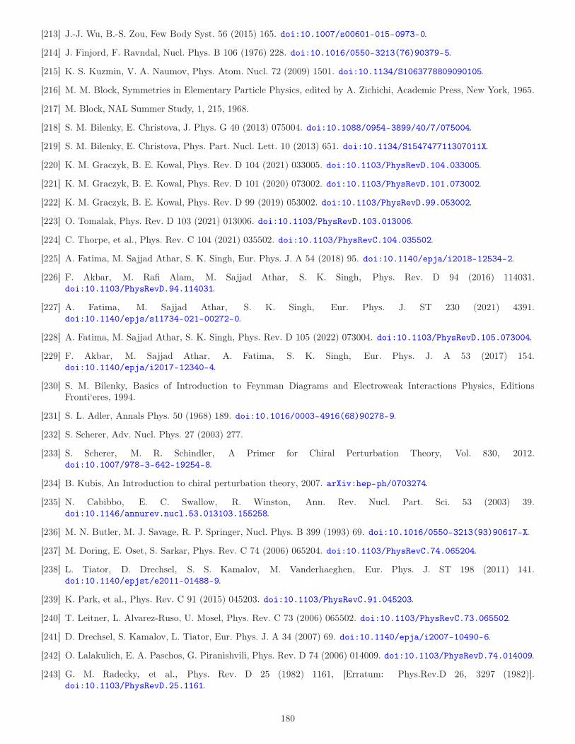
[213] J.-J. Wu, B.-S. Zou, Few Body Syst. 56 (2015) 165. doi:10.1007/s00601-015-0973-0.

[214] J. Finjord, F. Ravndal, Nucl. Phys. B 106 (1976) 228. doi:10.1016/0550-3213(76)90379-5.

[215] K. S. Kuzmin, V. A. Naumov, Phys. Atom. Nucl. 72 (2009) 1501. doi:10.1134/S1063778809090105.

[216] M. M. Block, Symmetries in Elementary Particle Physics, edited by A. Zichichi, Academic Press, New York, 1965.

[217] M. Block, NAL Summer Study, 1, 215, 1968.

[218] S. M. Bilenky, E. Christova, J. Phys. G 40 (2013) 075004. doi:10.1088/0954-3899/40/7/075004.

[219] S. M. Bilenky, E. Christova, Phys. Part. Nucl. Lett. 10 (2013) 651. doi:10.1134/S154747711307011X.

[220] K. M. Graczyk, B. E. Kowal, Phys. Rev. D 104 (2021) 033005. doi:10.1103/PhysRevD.104.033005.

[221] K. M. Graczyk, B. E. Kowal, Phys. Rev. D 101 (2020) 073002. doi:10.1103/PhysRevD.101.073002.

[222] K. M. Graczyk, B. E. Kowal, Phys. Rev. D 99 (2019) 053002. doi:10.1103/PhysRevD.99.053002.

[223] O. Tomalak, Phys. Rev. D 103 (2021) 013006. doi:10.1103/PhysRevD.103.013006.

[224] C. Thorpe, et al., Phys. Rev. C 104 (2021) 035502. doi:10.1103/PhysRevC.104.035502.

[225] A. Fatima, M. Sajjad Athar, S. K. Singh, Eur. Phys. J. A 54 (2018) 95. doi:10.1140/epja/i2018-12534-2.

[226] F. Akbar, M. Rafi Alam, M. Sajjad Athar, S. K. Singh, Phys. Rev. D 94 (2016) 114031.doi:10.1103/PhysRevD.94.114031.

[227] A. Fatima, M. Sajjad Athar, S. K. Singh, Eur. Phys. J. ST 230 (2021) 4391.doi:10.1140/epjs/s11734-021-00272-0.

[228] A. Fatima, M. Sajjad Athar, S. K. Singh, Phys. Rev. D 105 (2022) 073004. doi:10.1103/PhysRevD.105.073004.

[229] F. Akbar, M. Sajjad Athar, A. Fatima, S. K. Singh, Eur. Phys. J. A 53 (2017) 154.doi:10.1140/epja/i2017-12340-4.

[230] S. M. Bilenky, Basics of Introduction to Feynman Diagrams and Electroweak Interactions Physics, EditionsFronti‘eres, 1994.

[231] S. L. Adler, Annals Phys. 50 (1968) 189. doi:10.1016/0003-4916(68)90278-9.

[232] S. Scherer, Adv. Nucl. Phys. 27 (2003) 277.

[233] S. Scherer, M. R. Schindler, A Primer for Chiral Perturbation Theory, Vol. 830, 2012.doi:10.1007/978-3-642-19254-8.

[234] B. Kubis, An Introduction to chiral perturbation theory, 2007. arXiv:hep-ph/0703274.

[235] N. Cabibbo, E. C. Swallow, R. Winston, Ann. Rev. Nucl. Part. Sci. 53 (2003) 39.doi:10.1146/annurev.nucl.53.013103.155258.

[236] M. N. Butler, M. J. Savage, R. P. Springer, Nucl. Phys. B 399 (1993) 69. doi:10.1016/0550-3213(93)90617-X.

[237] M. Doring, E. Oset, S. Sarkar, Phys. Rev. C 74 (2006) 065204. doi:10.1103/PhysRevC.74.065204.

[238] L. Tiator, D. Drechsel, S. S. Kamalov, M. Vanderhaeghen, Eur. Phys. J. ST 198 (2011) 141.doi:10.1140/epjst/e2011-01488-9.

[239] K. Park, et al., Phys. Rev. C 91 (2015) 045203. doi:10.1103/PhysRevC.91.045203.

[240] T. Leitner, L. Alvarez-Ruso, U. Mosel, Phys. Rev. C 73 (2006) 065502. doi:10.1103/PhysRevC.73.065502.

[241] D. Drechsel, S. Kamalov, L. Tiator, Eur. Phys. J. A 34 (2007) 69. doi:10.1140/epja/i2007-10490-6.

[242] O. Lalakulich, E. A. Paschos, G. Piranishvili, Phys. Rev. D 74 (2006) 014009. doi:10.1103/PhysRevD.74.014009.

[243] G. M. Radecky, et al., Phys. Rev. D 25 (1982) 1161, [Erratum: Phys.Rev.D 26, 3297 (1982)].doi:10.1103/PhysRevD.25.1161.

180

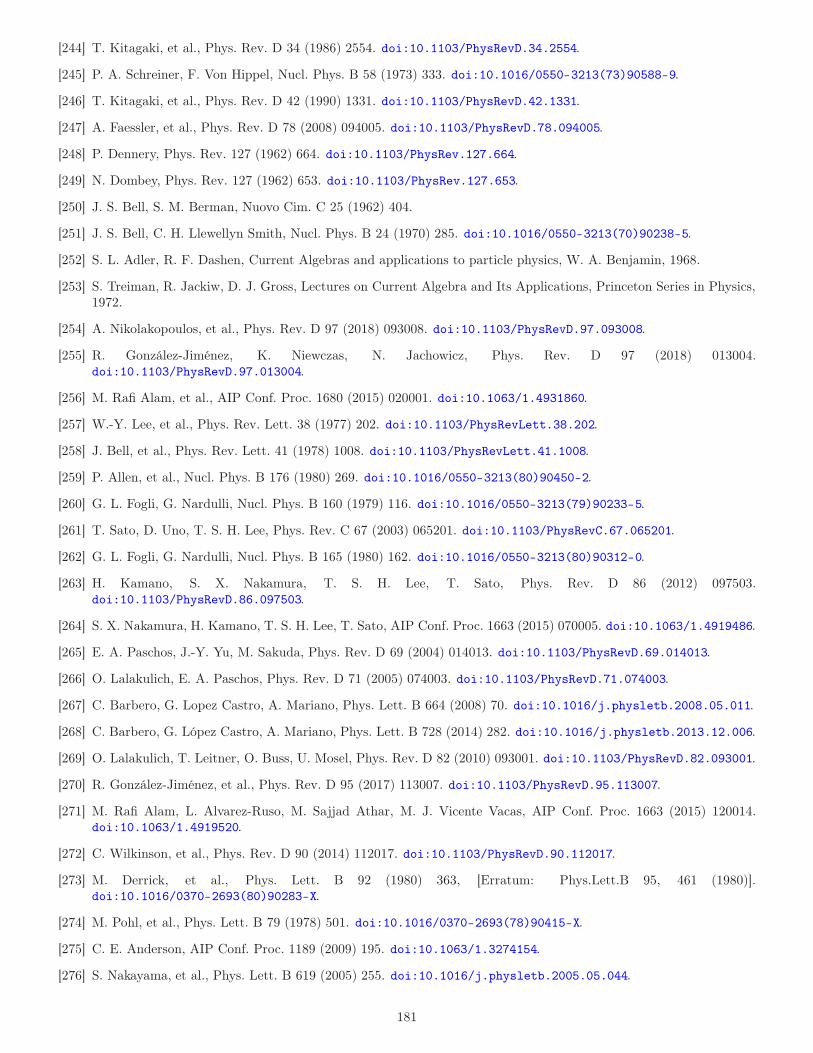
[244] T. Kitagaki, et al., Phys. Rev. D 34 (1986) 2554. doi:10.1103/PhysRevD.34.2554.

[245] P. A. Schreiner, F. Von Hippel, Nucl. Phys. B 58 (1973) 333. doi:10.1016/0550-3213(73)90588-9.

[246] T. Kitagaki, et al., Phys. Rev. D 42 (1990) 1331. doi:10.1103/PhysRevD.42.1331.

[247] A. Faessler, et al., Phys. Rev. D 78 (2008) 094005. doi:10.1103/PhysRevD.78.094005.

[248] P. Dennery, Phys. Rev. 127 (1962) 664. doi:10.1103/PhysRev.127.664.

[249] N. Dombey, Phys. Rev. 127 (1962) 653. doi:10.1103/PhysRev.127.653.

[250] J. S. Bell, S. M. Berman, Nuovo Cim. C 25 (1962) 404.

[251] J. S. Bell, C. H. Llewellyn Smith, Nucl. Phys. B 24 (1970) 285. doi:10.1016/0550-3213(70)90238-5.

[252] S. L. Adler, R. F. Dashen, Current Algebras and applications to particle physics, W. A. Benjamin, 1968.

[253] S. Treiman, R. Jackiw, D. J. Gross, Lectures on Current Algebra and Its Applications, Princeton Series in Physics,1972.

[254] A. Nikolakopoulos, et al., Phys. Rev. D 97 (2018) 093008. doi:10.1103/PhysRevD.97.093008.

[255] R. González-Jiménez, K. Niewczas, N. Jachowicz, Phys. Rev. D 97 (2018) 013004.doi:10.1103/PhysRevD.97.013004.

[256] M. Rafi Alam, et al., AIP Conf. Proc. 1680 (2015) 020001. doi:10.1063/1.4931860.

[257] W.-Y. Lee, et al., Phys. Rev. Lett. 38 (1977) 202. doi:10.1103/PhysRevLett.38.202.

[258] J. Bell, et al., Phys. Rev. Lett. 41 (1978) 1008. doi:10.1103/PhysRevLett.41.1008.

[259] P. Allen, et al., Nucl. Phys. B 176 (1980) 269. doi:10.1016/0550-3213(80)90450-2.

[260] G. L. Fogli, G. Nardulli, Nucl. Phys. B 160 (1979) 116. doi:10.1016/0550-3213(79)90233-5.

[261] T. Sato, D. Uno, T. S. H. Lee, Phys. Rev. C 67 (2003) 065201. doi:10.1103/PhysRevC.67.065201.

[262] G. L. Fogli, G. Nardulli, Nucl. Phys. B 165 (1980) 162. doi:10.1016/0550-3213(80)90312-0.

[263] H. Kamano, S. X. Nakamura, T. S. H. Lee, T. Sato, Phys. Rev. D 86 (2012) 097503.doi:10.1103/PhysRevD.86.097503.

[264] S. X. Nakamura, H. Kamano, T. S. H. Lee, T. Sato, AIP Conf. Proc. 1663 (2015) 070005. doi:10.1063/1.4919486.

[265] E. A. Paschos, J.-Y. Yu, M. Sakuda, Phys. Rev. D 69 (2004) 014013. doi:10.1103/PhysRevD.69.014013.

[266] O. Lalakulich, E. A. Paschos, Phys. Rev. D 71 (2005) 074003. doi:10.1103/PhysRevD.71.074003.

[267] C. Barbero, G. Lopez Castro, A. Mariano, Phys. Lett. B 664 (2008) 70. doi:10.1016/j.physletb.2008.05.011.

[268] C. Barbero, G. López Castro, A. Mariano, Phys. Lett. B 728 (2014) 282. doi:10.1016/j.physletb.2013.12.006.

[269] O. Lalakulich, T. Leitner, O. Buss, U. Mosel, Phys. Rev. D 82 (2010) 093001. doi:10.1103/PhysRevD.82.093001.

[270] R. González-Jiménez, et al., Phys. Rev. D 95 (2017) 113007. doi:10.1103/PhysRevD.95.113007.

[271] M. Rafi Alam, L. Alvarez-Ruso, M. Sajjad Athar, M. J. Vicente Vacas, AIP Conf. Proc. 1663 (2015) 120014.doi:10.1063/1.4919520.

[272] C. Wilkinson, et al., Phys. Rev. D 90 (2014) 112017. doi:10.1103/PhysRevD.90.112017.

[273] M. Derrick, et al., Phys. Lett. B 92 (1980) 363, [Erratum: Phys.Lett.B 95, 461 (1980)].doi:10.1016/0370-2693(80)90283-X.

[274] M. Pohl, et al., Phys. Lett. B 79 (1978) 501. doi:10.1016/0370-2693(78)90415-X.

[275] C. E. Anderson, AIP Conf. Proc. 1189 (2009) 195. doi:10.1063/1.3274154.

[276] S. Nakayama, et al., Phys. Lett. B 619 (2005) 255. doi:10.1016/j.physletb.2005.05.044.

181

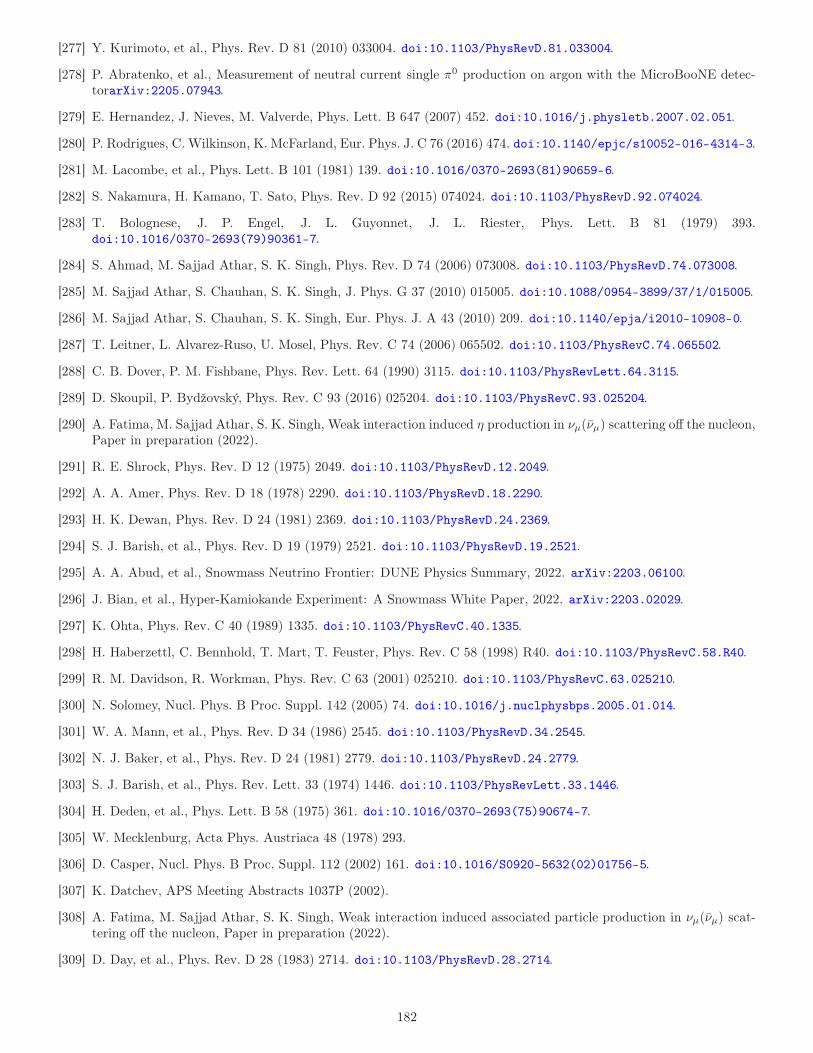
[277] Y. Kurimoto, et al., Phys. Rev. D 81 (2010) 033004. doi:10.1103/PhysRevD.81.033004.

[278] P. Abratenko, et al., Measurement of neutral current single π0 production on argon with the MicroBooNE detec-torarXiv:2205.07943.

[279] E. Hernandez, J. Nieves, M. Valverde, Phys. Lett. B 647 (2007) 452. doi:10.1016/j.physletb.2007.02.051.

[280] P. Rodrigues, C. Wilkinson, K. McFarland, Eur. Phys. J. C 76 (2016) 474. doi:10.1140/epjc/s10052-016-4314-3.

[281] M. Lacombe, et al., Phys. Lett. B 101 (1981) 139. doi:10.1016/0370-2693(81)90659-6.

[282] S. Nakamura, H. Kamano, T. Sato, Phys. Rev. D 92 (2015) 074024. doi:10.1103/PhysRevD.92.074024.

[283] T. Bolognese, J. P. Engel, J. L. Guyonnet, J. L. Riester, Phys. Lett. B 81 (1979) 393.doi:10.1016/0370-2693(79)90361-7.

[284] S. Ahmad, M. Sajjad Athar, S. K. Singh, Phys. Rev. D 74 (2006) 073008. doi:10.1103/PhysRevD.74.073008.

[285] M. Sajjad Athar, S. Chauhan, S. K. Singh, J. Phys. G 37 (2010) 015005. doi:10.1088/0954-3899/37/1/015005.

[286] M. Sajjad Athar, S. Chauhan, S. K. Singh, Eur. Phys. J. A 43 (2010) 209. doi:10.1140/epja/i2010-10908-0.

[287] T. Leitner, L. Alvarez-Ruso, U. Mosel, Phys. Rev. C 74 (2006) 065502. doi:10.1103/PhysRevC.74.065502.

[288] C. B. Dover, P. M. Fishbane, Phys. Rev. Lett. 64 (1990) 3115. doi:10.1103/PhysRevLett.64.3115.

[289] D. Skoupil, P. Bydžovský, Phys. Rev. C 93 (2016) 025204. doi:10.1103/PhysRevC.93.025204.

[290] A. Fatima, M. Sajjad Athar, S. K. Singh, Weak interaction induced η production in νµ(νµ) scattering off the nucleon,Paper in preparation (2022).

[291] R. E. Shrock, Phys. Rev. D 12 (1975) 2049. doi:10.1103/PhysRevD.12.2049.

[292] A. A. Amer, Phys. Rev. D 18 (1978) 2290. doi:10.1103/PhysRevD.18.2290.

[293] H. K. Dewan, Phys. Rev. D 24 (1981) 2369. doi:10.1103/PhysRevD.24.2369.

[294] S. J. Barish, et al., Phys. Rev. D 19 (1979) 2521. doi:10.1103/PhysRevD.19.2521.

[295] A. A. Abud, et al., Snowmass Neutrino Frontier: DUNE Physics Summary, 2022. arXiv:2203.06100.

[296] J. Bian, et al., Hyper-Kamiokande Experiment: A Snowmass White Paper, 2022. arXiv:2203.02029.

[297] K. Ohta, Phys. Rev. C 40 (1989) 1335. doi:10.1103/PhysRevC.40.1335.

[298] H. Haberzettl, C. Bennhold, T. Mart, T. Feuster, Phys. Rev. C 58 (1998) R40. doi:10.1103/PhysRevC.58.R40.

[299] R. M. Davidson, R. Workman, Phys. Rev. C 63 (2001) 025210. doi:10.1103/PhysRevC.63.025210.

[300] N. Solomey, Nucl. Phys. B Proc. Suppl. 142 (2005) 74. doi:10.1016/j.nuclphysbps.2005.01.014.

[301] W. A. Mann, et al., Phys. Rev. D 34 (1986) 2545. doi:10.1103/PhysRevD.34.2545.

[302] N. J. Baker, et al., Phys. Rev. D 24 (1981) 2779. doi:10.1103/PhysRevD.24.2779.

[303] S. J. Barish, et al., Phys. Rev. Lett. 33 (1974) 1446. doi:10.1103/PhysRevLett.33.1446.

[304] H. Deden, et al., Phys. Lett. B 58 (1975) 361. doi:10.1016/0370-2693(75)90674-7.

[305] W. Mecklenburg, Acta Phys. Austriaca 48 (1978) 293.

[306] D. Casper, Nucl. Phys. B Proc. Suppl. 112 (2002) 161. doi:10.1016/S0920-5632(02)01756-5.

[307] K. Datchev, APS Meeting Abstracts 1037P (2002).

[308] A. Fatima, M. Sajjad Athar, S. K. Singh, Weak interaction induced associated particle production in νµ(νµ) scat-tering off the nucleon, Paper in preparation (2022).

[309] D. Day, et al., Phys. Rev. D 28 (1983) 2714. doi:10.1103/PhysRevD.28.2714.

182

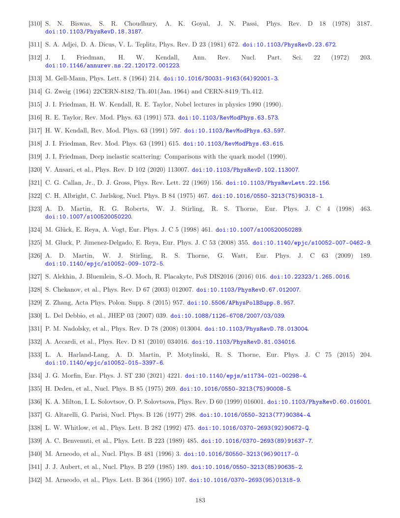
[310] S. N. Biswas, S. R. Choudhury, A. K. Goyal, J. N. Passi, Phys. Rev. D 18 (1978) 3187.doi:10.1103/PhysRevD.18.3187.

[311] S. A. Adjei, D. A. Dicus, V. L. Teplitz, Phys. Rev. D 23 (1981) 672. doi:10.1103/PhysRevD.23.672.

[312] J. I. Friedman, H. W. Kendall, Ann. Rev. Nucl. Part. Sci. 22 (1972) 203.doi:10.1146/annurev.ns.22.120172.001223.

[313] M. Gell-Mann, Phys. Lett. 8 (1964) 214. doi:10.1016/S0031-9163(64)92001-3.

[314] G. Zweig (1964) 22CERN-8182/Th.401(Jan. 1964) and CERN-8419/Th.412.

[315] J. I. Friedman, H. W. Kendall, R. E. Taylor, Nobel lectures in physics 1990 (1990).

[316] R. E. Taylor, Rev. Mod. Phys. 63 (1991) 573. doi:10.1103/RevModPhys.63.573.

[317] H. W. Kendall, Rev. Mod. Phys. 63 (1991) 597. doi:10.1103/RevModPhys.63.597.

[318] J. I. Friedman, Rev. Mod. Phys. 63 (1991) 615. doi:10.1103/RevModPhys.63.615.

[319] J. I. Friedman, Deep inelastic scattering: Comparisons with the quark model (1990).

[320] V. Ansari, et al., Phys. Rev. D 102 (2020) 113007. doi:10.1103/PhysRevD.102.113007.

[321] C. G. Callan, Jr., D. J. Gross, Phys. Rev. Lett. 22 (1969) 156. doi:10.1103/PhysRevLett.22.156.

[322] C. H. Albright, C. Jarlskog, Nucl. Phys. B 84 (1975) 467. doi:10.1016/0550-3213(75)90318-1.

[323] A. D. Martin, R. G. Roberts, W. J. Stirling, R. S. Thorne, Eur. Phys. J. C 4 (1998) 463.doi:10.1007/s100520050220.

[324] M. Glück, E. Reya, A. Vogt, Eur. Phys. J. C 5 (1998) 461. doi:10.1007/s100520050289.

[325] M. Gluck, P. Jimenez-Delgado, E. Reya, Eur. Phys. J. C 53 (2008) 355. doi:10.1140/epjc/s10052-007-0462-9.

[326] A. D. Martin, W. J. Stirling, R. S. Thorne, G. Watt, Eur. Phys. J. C 63 (2009) 189.doi:10.1140/epjc/s10052-009-1072-5.

[327] S. Alekhin, J. Bluemlein, S.-O. Moch, R. Placakyte, PoS DIS2016 (2016) 016. doi:10.22323/1.265.0016.

[328] S. Chekanov, et al., Phys. Rev. D 67 (2003) 012007. doi:10.1103/PhysRevD.67.012007.

[329] Z. Zhang, Acta Phys. Polon. Supp. 8 (2015) 957. doi:10.5506/APhysPolBSupp.8.957.

[330] L. Del Debbio, et al., JHEP 03 (2007) 039. doi:10.1088/1126-6708/2007/03/039.

[331] P. M. Nadolsky, et al., Phys. Rev. D 78 (2008) 013004. doi:10.1103/PhysRevD.78.013004.

[332] A. Accardi, et al., Phys. Rev. D 81 (2010) 034016. doi:10.1103/PhysRevD.81.034016.

[333] L. A. Harland-Lang, A. D. Martin, P. Motylinski, R. S. Thorne, Eur. Phys. J. C 75 (2015) 204.doi:10.1140/epjc/s10052-015-3397-6.

[334] J. G. Morfin, Eur. Phys. J. ST 230 (2021) 4221. doi:10.1140/epjs/s11734-021-00298-4.

[335] H. Deden, et al., Nucl. Phys. B 85 (1975) 269. doi:10.1016/0550-3213(75)90008-5.

[336] K. A. Milton, I. L. Solovtsov, O. P. Solovtsova, Phys. Rev. D 60 (1999) 016001. doi:10.1103/PhysRevD.60.016001.

[337] G. Altarelli, G. Parisi, Nucl. Phys. B 126 (1977) 298. doi:10.1016/0550-3213(77)90384-4.

[338] L. W. Whitlow, et al., Phys. Lett. B 282 (1992) 475. doi:10.1016/0370-2693(92)90672-Q.

[339] A. C. Benvenuti, et al., Phys. Lett. B 223 (1989) 485. doi:10.1016/0370-2693(89)91637-7.

[340] M. Arneodo, et al., Nucl. Phys. B 481 (1996) 3. doi:10.1016/S0550-3213(96)90117-0.

[341] J. J. Aubert, et al., Nucl. Phys. B 259 (1985) 189. doi:10.1016/0550-3213(85)90635-2.

[342] M. Arneodo, et al., Phys. Lett. B 364 (1995) 107. doi:10.1016/0370-2693(95)01318-9.

183

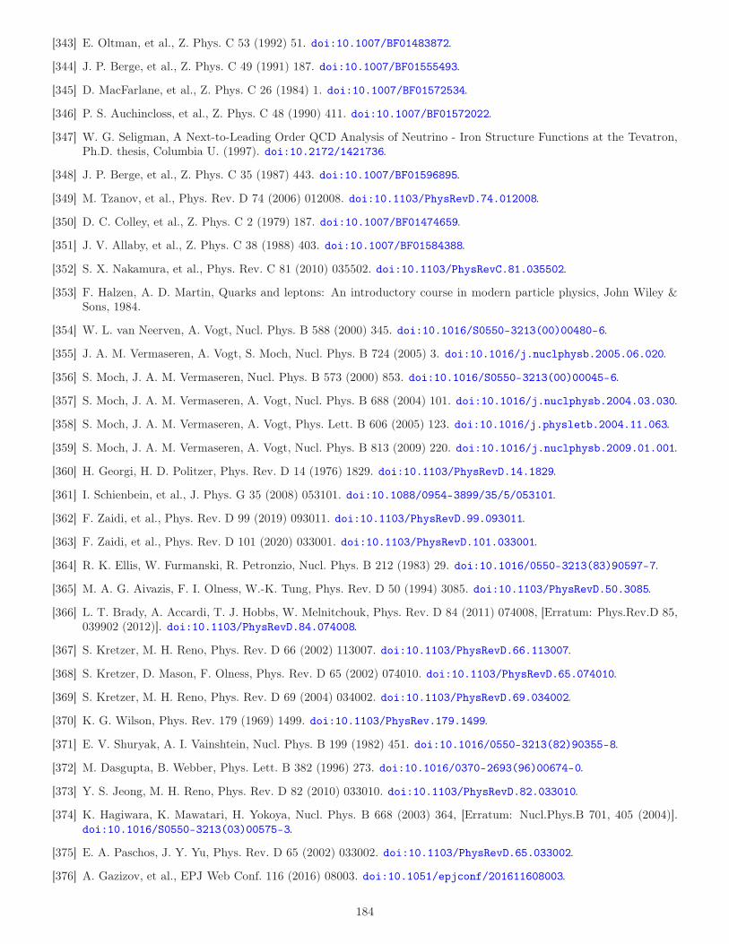
[343] E. Oltman, et al., Z. Phys. C 53 (1992) 51. doi:10.1007/BF01483872.

[344] J. P. Berge, et al., Z. Phys. C 49 (1991) 187. doi:10.1007/BF01555493.

[345] D. MacFarlane, et al., Z. Phys. C 26 (1984) 1. doi:10.1007/BF01572534.

[346] P. S. Auchincloss, et al., Z. Phys. C 48 (1990) 411. doi:10.1007/BF01572022.

[347] W. G. Seligman, A Next-to-Leading Order QCD Analysis of Neutrino - Iron Structure Functions at the Tevatron,Ph.D. thesis, Columbia U. (1997). doi:10.2172/1421736.

[348] J. P. Berge, et al., Z. Phys. C 35 (1987) 443. doi:10.1007/BF01596895.

[349] M. Tzanov, et al., Phys. Rev. D 74 (2006) 012008. doi:10.1103/PhysRevD.74.012008.

[350] D. C. Colley, et al., Z. Phys. C 2 (1979) 187. doi:10.1007/BF01474659.

[351] J. V. Allaby, et al., Z. Phys. C 38 (1988) 403. doi:10.1007/BF01584388.

[352] S. X. Nakamura, et al., Phys. Rev. C 81 (2010) 035502. doi:10.1103/PhysRevC.81.035502.

[353] F. Halzen, A. D. Martin, Quarks and leptons: An introductory course in modern particle physics, John Wiley &Sons, 1984.

[354] W. L. van Neerven, A. Vogt, Nucl. Phys. B 588 (2000) 345. doi:10.1016/S0550-3213(00)00480-6.

[355] J. A. M. Vermaseren, A. Vogt, S. Moch, Nucl. Phys. B 724 (2005) 3. doi:10.1016/j.nuclphysb.2005.06.020.

[356] S. Moch, J. A. M. Vermaseren, Nucl. Phys. B 573 (2000) 853. doi:10.1016/S0550-3213(00)00045-6.

[357] S. Moch, J. A. M. Vermaseren, A. Vogt, Nucl. Phys. B 688 (2004) 101. doi:10.1016/j.nuclphysb.2004.03.030.

[358] S. Moch, J. A. M. Vermaseren, A. Vogt, Phys. Lett. B 606 (2005) 123. doi:10.1016/j.physletb.2004.11.063.

[359] S. Moch, J. A. M. Vermaseren, A. Vogt, Nucl. Phys. B 813 (2009) 220. doi:10.1016/j.nuclphysb.2009.01.001.

[360] H. Georgi, H. D. Politzer, Phys. Rev. D 14 (1976) 1829. doi:10.1103/PhysRevD.14.1829.

[361] I. Schienbein, et al., J. Phys. G 35 (2008) 053101. doi:10.1088/0954-3899/35/5/053101.

[362] F. Zaidi, et al., Phys. Rev. D 99 (2019) 093011. doi:10.1103/PhysRevD.99.093011.

[363] F. Zaidi, et al., Phys. Rev. D 101 (2020) 033001. doi:10.1103/PhysRevD.101.033001.

[364] R. K. Ellis, W. Furmanski, R. Petronzio, Nucl. Phys. B 212 (1983) 29. doi:10.1016/0550-3213(83)90597-7.

[365] M. A. G. Aivazis, F. I. Olness, W.-K. Tung, Phys. Rev. D 50 (1994) 3085. doi:10.1103/PhysRevD.50.3085.

[366] L. T. Brady, A. Accardi, T. J. Hobbs, W. Melnitchouk, Phys. Rev. D 84 (2011) 074008, [Erratum: Phys.Rev.D 85,039902 (2012)]. doi:10.1103/PhysRevD.84.074008.

[367] S. Kretzer, M. H. Reno, Phys. Rev. D 66 (2002) 113007. doi:10.1103/PhysRevD.66.113007.

[368] S. Kretzer, D. Mason, F. Olness, Phys. Rev. D 65 (2002) 074010. doi:10.1103/PhysRevD.65.074010.

[369] S. Kretzer, M. H. Reno, Phys. Rev. D 69 (2004) 034002. doi:10.1103/PhysRevD.69.034002.

[370] K. G. Wilson, Phys. Rev. 179 (1969) 1499. doi:10.1103/PhysRev.179.1499.

[371] E. V. Shuryak, A. I. Vainshtein, Nucl. Phys. B 199 (1982) 451. doi:10.1016/0550-3213(82)90355-8.

[372] M. Dasgupta, B. Webber, Phys. Lett. B 382 (1996) 273. doi:10.1016/0370-2693(96)00674-0.

[373] Y. S. Jeong, M. H. Reno, Phys. Rev. D 82 (2010) 033010. doi:10.1103/PhysRevD.82.033010.

[374] K. Hagiwara, K. Mawatari, H. Yokoya, Nucl. Phys. B 668 (2003) 364, [Erratum: Nucl.Phys.B 701, 405 (2004)].doi:10.1016/S0550-3213(03)00575-3.

[375] E. A. Paschos, J. Y. Yu, Phys. Rev. D 65 (2002) 033002. doi:10.1103/PhysRevD.65.033002.

[376] A. Gazizov, et al., EPJ Web Conf. 116 (2016) 08003. doi:10.1051/epjconf/201611608003.

184

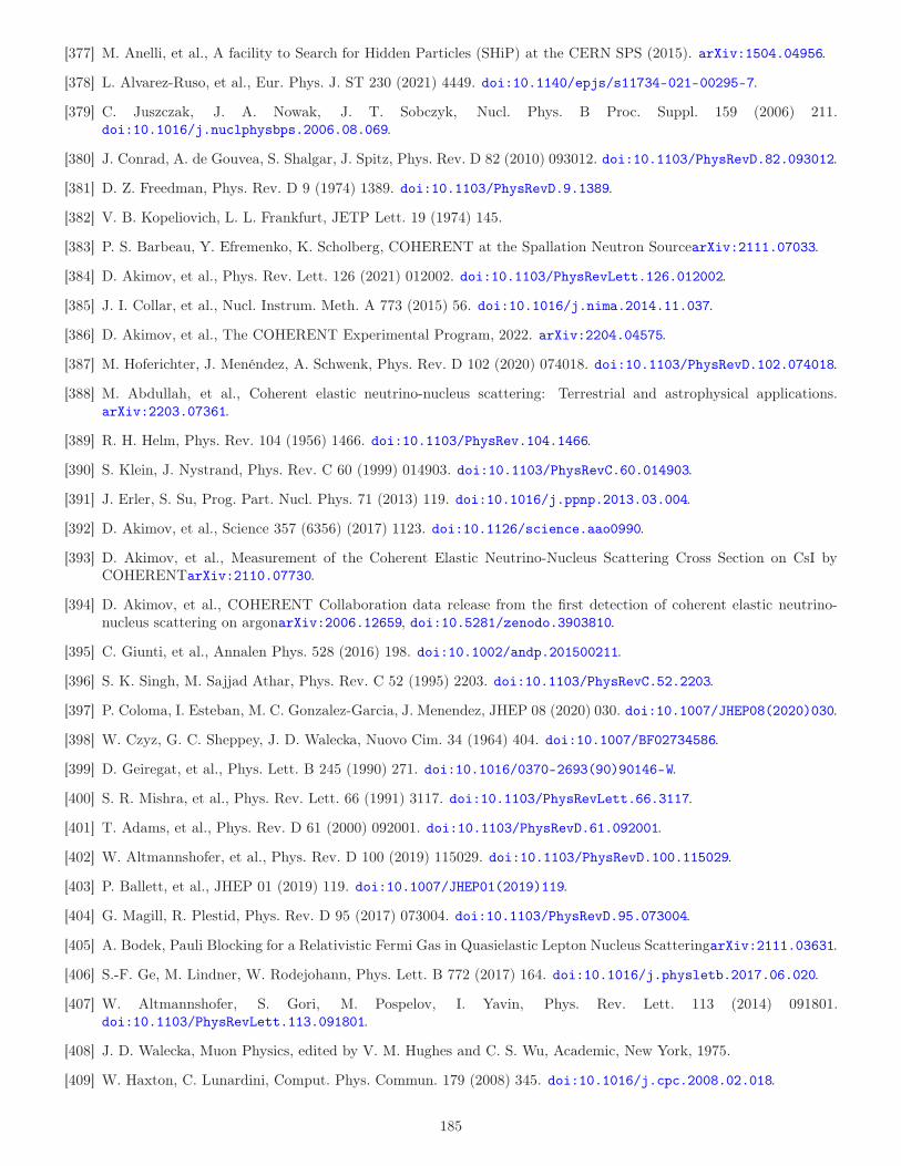
[377] M. Anelli, et al., A facility to Search for Hidden Particles (SHiP) at the CERN SPS (2015). arXiv:1504.04956.

[378] L. Alvarez-Ruso, et al., Eur. Phys. J. ST 230 (2021) 4449. doi:10.1140/epjs/s11734-021-00295-7.

[379] C. Juszczak, J. A. Nowak, J. T. Sobczyk, Nucl. Phys. B Proc. Suppl. 159 (2006) 211.doi:10.1016/j.nuclphysbps.2006.08.069.

[380] J. Conrad, A. de Gouvea, S. Shalgar, J. Spitz, Phys. Rev. D 82 (2010) 093012. doi:10.1103/PhysRevD.82.093012.

[381] D. Z. Freedman, Phys. Rev. D 9 (1974) 1389. doi:10.1103/PhysRevD.9.1389.

[382] V. B. Kopeliovich, L. L. Frankfurt, JETP Lett. 19 (1974) 145.

[383] P. S. Barbeau, Y. Efremenko, K. Scholberg, COHERENT at the Spallation Neutron SourcearXiv:2111.07033.

[384] D. Akimov, et al., Phys. Rev. Lett. 126 (2021) 012002. doi:10.1103/PhysRevLett.126.012002.

[385] J. I. Collar, et al., Nucl. Instrum. Meth. A 773 (2015) 56. doi:10.1016/j.nima.2014.11.037.

[386] D. Akimov, et al., The COHERENT Experimental Program, 2022. arXiv:2204.04575.

[387] M. Hoferichter, J. Menéndez, A. Schwenk, Phys. Rev. D 102 (2020) 074018. doi:10.1103/PhysRevD.102.074018.

[388] M. Abdullah, et al., Coherent elastic neutrino-nucleus scattering: Terrestrial and astrophysical applications.arXiv:2203.07361.

[389] R. H. Helm, Phys. Rev. 104 (1956) 1466. doi:10.1103/PhysRev.104.1466.

[390] S. Klein, J. Nystrand, Phys. Rev. C 60 (1999) 014903. doi:10.1103/PhysRevC.60.014903.

[391] J. Erler, S. Su, Prog. Part. Nucl. Phys. 71 (2013) 119. doi:10.1016/j.ppnp.2013.03.004.

[392] D. Akimov, et al., Science 357 (6356) (2017) 1123. doi:10.1126/science.aao0990.

[393] D. Akimov, et al., Measurement of the Coherent Elastic Neutrino-Nucleus Scattering Cross Section on CsI byCOHERENTarXiv:2110.07730.

[394] D. Akimov, et al., COHERENT Collaboration data release from the first detection of coherent elastic neutrino-nucleus scattering on argonarXiv:2006.12659, doi:10.5281/zenodo.3903810.

[395] C. Giunti, et al., Annalen Phys. 528 (2016) 198. doi:10.1002/andp.201500211.

[396] S. K. Singh, M. Sajjad Athar, Phys. Rev. C 52 (1995) 2203. doi:10.1103/PhysRevC.52.2203.

[397] P. Coloma, I. Esteban, M. C. Gonzalez-Garcia, J. Menendez, JHEP 08 (2020) 030. doi:10.1007/JHEP08(2020)030.

[398] W. Czyz, G. C. Sheppey, J. D. Walecka, Nuovo Cim. 34 (1964) 404. doi:10.1007/BF02734586.

[399] D. Geiregat, et al., Phys. Lett. B 245 (1990) 271. doi:10.1016/0370-2693(90)90146-W.

[400] S. R. Mishra, et al., Phys. Rev. Lett. 66 (1991) 3117. doi:10.1103/PhysRevLett.66.3117.

[401] T. Adams, et al., Phys. Rev. D 61 (2000) 092001. doi:10.1103/PhysRevD.61.092001.

[402] W. Altmannshofer, et al., Phys. Rev. D 100 (2019) 115029. doi:10.1103/PhysRevD.100.115029.

[403] P. Ballett, et al., JHEP 01 (2019) 119. doi:10.1007/JHEP01(2019)119.

[404] G. Magill, R. Plestid, Phys. Rev. D 95 (2017) 073004. doi:10.1103/PhysRevD.95.073004.

[405] A. Bodek, Pauli Blocking for a Relativistic Fermi Gas in Quasielastic Lepton Nucleus ScatteringarXiv:2111.03631.

[406] S.-F. Ge, M. Lindner, W. Rodejohann, Phys. Lett. B 772 (2017) 164. doi:10.1016/j.physletb.2017.06.020.

[407] W. Altmannshofer, S. Gori, M. Pospelov, I. Yavin, Phys. Rev. Lett. 113 (2014) 091801.doi:10.1103/PhysRevLett.113.091801.

[408] J. D. Walecka, Muon Physics, edited by V. M. Hughes and C. S. Wu, Academic, New York, 1975.

[409] W. Haxton, C. Lunardini, Comput. Phys. Commun. 179 (2008) 345. doi:10.1016/j.cpc.2008.02.018.

185

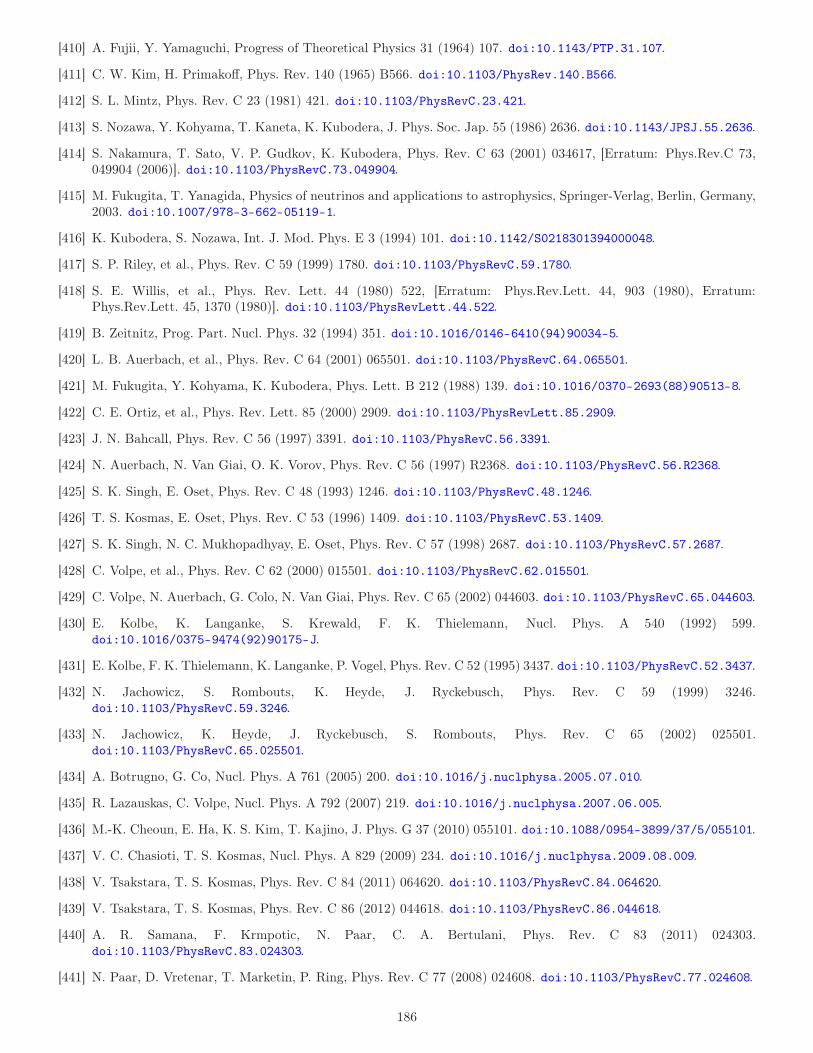
[410] A. Fujii, Y. Yamaguchi, Progress of Theoretical Physics 31 (1964) 107. doi:10.1143/PTP.31.107.

[411] C. W. Kim, H. Primakoff, Phys. Rev. 140 (1965) B566. doi:10.1103/PhysRev.140.B566.

[412] S. L. Mintz, Phys. Rev. C 23 (1981) 421. doi:10.1103/PhysRevC.23.421.

[413] S. Nozawa, Y. Kohyama, T. Kaneta, K. Kubodera, J. Phys. Soc. Jap. 55 (1986) 2636. doi:10.1143/JPSJ.55.2636.

[414] S. Nakamura, T. Sato, V. P. Gudkov, K. Kubodera, Phys. Rev. C 63 (2001) 034617, [Erratum: Phys.Rev.C 73,049904 (2006)]. doi:10.1103/PhysRevC.73.049904.

[415] M. Fukugita, T. Yanagida, Physics of neutrinos and applications to astrophysics, Springer-Verlag, Berlin, Germany,2003. doi:10.1007/978-3-662-05119-1.

[416] K. Kubodera, S. Nozawa, Int. J. Mod. Phys. E 3 (1994) 101. doi:10.1142/S0218301394000048.

[417] S. P. Riley, et al., Phys. Rev. C 59 (1999) 1780. doi:10.1103/PhysRevC.59.1780.

[418] S. E. Willis, et al., Phys. Rev. Lett. 44 (1980) 522, [Erratum: Phys.Rev.Lett. 44, 903 (1980), Erratum:Phys.Rev.Lett. 45, 1370 (1980)]. doi:10.1103/PhysRevLett.44.522.

[419] B. Zeitnitz, Prog. Part. Nucl. Phys. 32 (1994) 351. doi:10.1016/0146-6410(94)90034-5.

[420] L. B. Auerbach, et al., Phys. Rev. C 64 (2001) 065501. doi:10.1103/PhysRevC.64.065501.

[421] M. Fukugita, Y. Kohyama, K. Kubodera, Phys. Lett. B 212 (1988) 139. doi:10.1016/0370-2693(88)90513-8.

[422] C. E. Ortiz, et al., Phys. Rev. Lett. 85 (2000) 2909. doi:10.1103/PhysRevLett.85.2909.

[423] J. N. Bahcall, Phys. Rev. C 56 (1997) 3391. doi:10.1103/PhysRevC.56.3391.

[424] N. Auerbach, N. Van Giai, O. K. Vorov, Phys. Rev. C 56 (1997) R2368. doi:10.1103/PhysRevC.56.R2368.

[425] S. K. Singh, E. Oset, Phys. Rev. C 48 (1993) 1246. doi:10.1103/PhysRevC.48.1246.

[426] T. S. Kosmas, E. Oset, Phys. Rev. C 53 (1996) 1409. doi:10.1103/PhysRevC.53.1409.

[427] S. K. Singh, N. C. Mukhopadhyay, E. Oset, Phys. Rev. C 57 (1998) 2687. doi:10.1103/PhysRevC.57.2687.

[428] C. Volpe, et al., Phys. Rev. C 62 (2000) 015501. doi:10.1103/PhysRevC.62.015501.

[429] C. Volpe, N. Auerbach, G. Colo, N. Van Giai, Phys. Rev. C 65 (2002) 044603. doi:10.1103/PhysRevC.65.044603.

[430] E. Kolbe, K. Langanke, S. Krewald, F. K. Thielemann, Nucl. Phys. A 540 (1992) 599.doi:10.1016/0375-9474(92)90175-J.

[431] E. Kolbe, F. K. Thielemann, K. Langanke, P. Vogel, Phys. Rev. C 52 (1995) 3437. doi:10.1103/PhysRevC.52.3437.

[432] N. Jachowicz, S. Rombouts, K. Heyde, J. Ryckebusch, Phys. Rev. C 59 (1999) 3246.doi:10.1103/PhysRevC.59.3246.

[433] N. Jachowicz, K. Heyde, J. Ryckebusch, S. Rombouts, Phys. Rev. C 65 (2002) 025501.doi:10.1103/PhysRevC.65.025501.

[434] A. Botrugno, G. Co, Nucl. Phys. A 761 (2005) 200. doi:10.1016/j.nuclphysa.2005.07.010.

[435] R. Lazauskas, C. Volpe, Nucl. Phys. A 792 (2007) 219. doi:10.1016/j.nuclphysa.2007.06.005.

[436] M.-K. Cheoun, E. Ha, K. S. Kim, T. Kajino, J. Phys. G 37 (2010) 055101. doi:10.1088/0954-3899/37/5/055101.

[437] V. C. Chasioti, T. S. Kosmas, Nucl. Phys. A 829 (2009) 234. doi:10.1016/j.nuclphysa.2009.08.009.

[438] V. Tsakstara, T. S. Kosmas, Phys. Rev. C 84 (2011) 064620. doi:10.1103/PhysRevC.84.064620.

[439] V. Tsakstara, T. S. Kosmas, Phys. Rev. C 86 (2012) 044618. doi:10.1103/PhysRevC.86.044618.

[440] A. R. Samana, F. Krmpotic, N. Paar, C. A. Bertulani, Phys. Rev. C 83 (2011) 024303.doi:10.1103/PhysRevC.83.024303.

[441] N. Paar, D. Vretenar, T. Marketin, P. Ring, Phys. Rev. C 77 (2008) 024608. doi:10.1103/PhysRevC.77.024608.

186

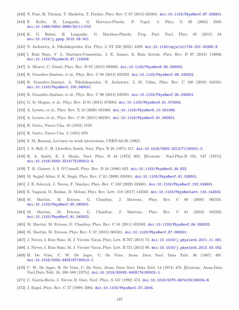
[442] N. Paar, H. Tutman, T. Marketin, T. Fischer, Phys. Rev. C 87 (2013) 025801. doi:10.1103/PhysRevC.87.025801.

[443] E. Kolbe, K. Langanke, G. Martinez-Pinedo, P. Vogel, J. Phys. G 29 (2003) 2569.doi:10.1088/0954-3899/29/11/010.

[444] K. G. Balasi, K. Langanke, G. Martínez-Pinedo, Prog. Part. Nucl. Phys. 85 (2015) 33.doi:10.1016/j.ppnp.2015.08.001.

[445] N. Jachowicz, A. Nikolakopoulos, Eur. Phys. J. ST 230 (2021) 4339. doi:10.1140/epjs/s11734-021-00286-8.

[446] I. Ruiz Simo, V. L. Martinez-Consentino, J. E. Amaro, E. Ruiz Arriola, Phys. Rev. D 97 (2018) 116006.doi:10.1103/PhysRevD.97.116006.

[447] A. Meucci, C. Giusti, Phys. Rev. D 85 (2012) 093002. doi:10.1103/PhysRevD.85.093002.

[448] R. González-Jiménez, et al., Phys. Rev. C 88 (2013) 025502. doi:10.1103/PhysRevC.88.025502.

[449] R. González-Jiménez, A. Nikolakopoulos, N. Jachowicz, J. M. Udías, Phys. Rev. C 100 (2019) 045501.doi:10.1103/PhysRevC.100.045501.

[450] R. Gonzaléz-Jiménez, et al., Phys. Rev. C 90 (2014) 035501. doi:10.1103/PhysRevC.90.035501.

[451] G. D. Megias, et al., Phys. Rev. D 91 (2015) 073004. doi:10.1103/PhysRevD.91.073004.

[452] A. Lovato, et al., Phys. Rev. X 10 (2020) 031068. doi:10.1103/PhysRevX.10.031068.

[453] A. Lovato, et al., Phys. Rev. C 91 (2015) 062501. doi:10.1103/PhysRevC.91.062501.

[454] R. Gatto, Nuovo Cim. 10 (1953) 1559.

[455] R. Gatto, Nuovo Cim. 2 (1955) 670.

[456] S. M. Berman, Lectures on weak interactions, CERN-62-20 (1962).

[457] J. S. Bell, C. H. Llewellyn Smith, Nucl. Phys. B 28 (1971) 317. doi:10.1016/0550-3213(71)90001-0.

[458] R. A. Smith, E. J. Moniz, Nucl. Phys. B 43 (1972) 605, [Erratum: Nucl.Phys.B 101, 547 (1975)].doi:10.1016/0550-3213(75)90612-4.

[459] T. K. Gaisser, J. S. O’Connell, Phys. Rev. D 34 (1986) 822. doi:10.1103/PhysRevD.34.822.

[460] M. Sajjad Athar, S. K. Singh, Phys. Rev. C 61 (2000) 028501. doi:10.1103/PhysRevC.61.028501.

[461] J. E. Sobczyk, J. Nieves, F. Sánchez, Phys. Rev. C 102 (2020) 024601. doi:10.1103/PhysRevC.102.024601.

[462] E. Vagnoni, O. Benhar, D. Meloni, Phys. Rev. Lett. 118 (2017) 142502. doi:10.1103/PhysRevLett.118.142502.

[463] M. Martini, M. Ericson, G. Chanfray, J. Marteau, Phys. Rev. C 80 (2009) 065501.doi:10.1103/PhysRevC.80.065501.

[464] M. Martini, M. Ericson, G. Chanfray, J. Marteau, Phys. Rev. C 81 (2010) 045502.doi:10.1103/PhysRevC.81.045502.

[465] M. Martini, M. Ericson, G. Chanfray, Phys. Rev. C 84 (2011) 055502. doi:10.1103/PhysRevC.84.055502.

[466] M. Martini, M. Ericson, Phys. Rev. C 87 (2013) 065501. doi:10.1103/PhysRevC.87.065501.

[467] J. Nieves, I. Ruiz Simo, M. J. Vicente Vacas, Phys. Lett. B 707 (2012) 72. doi:10.1016/j.physletb.2011.11.061.

[468] J. Nieves, I. Ruiz Simo, M. J. Vicente Vacas, Phys. Lett. B 721 (2013) 90. doi:10.1016/j.physletb.2013.03.002.

[469] H. De Vries, C. W. De Jager, C. De Vries, Atom. Data Nucl. Data Tabl. 36 (1987) 495.doi:10.1016/0092-640X(87)90013-1.

[470] C. W. De Jager, H. De Vries, C. De Vries, Atom. Data Nucl. Data Tabl. 14 (1974) 479, [Erratum: Atom.DataNucl.Data Tabl. 16, 580–580 (1975)]. doi:10.1016/S0092-640X(74)80002-1.

[471] C. Garcia-Recio, J. Nieves, E. Oset, Nucl. Phys. A 547 (1992) 473. doi:10.1016/0375-9474(92)90034-H.

[472] J. Engel, Phys. Rev. C 57 (1998) 2004. doi:10.1103/PhysRevC.57.2004.

187

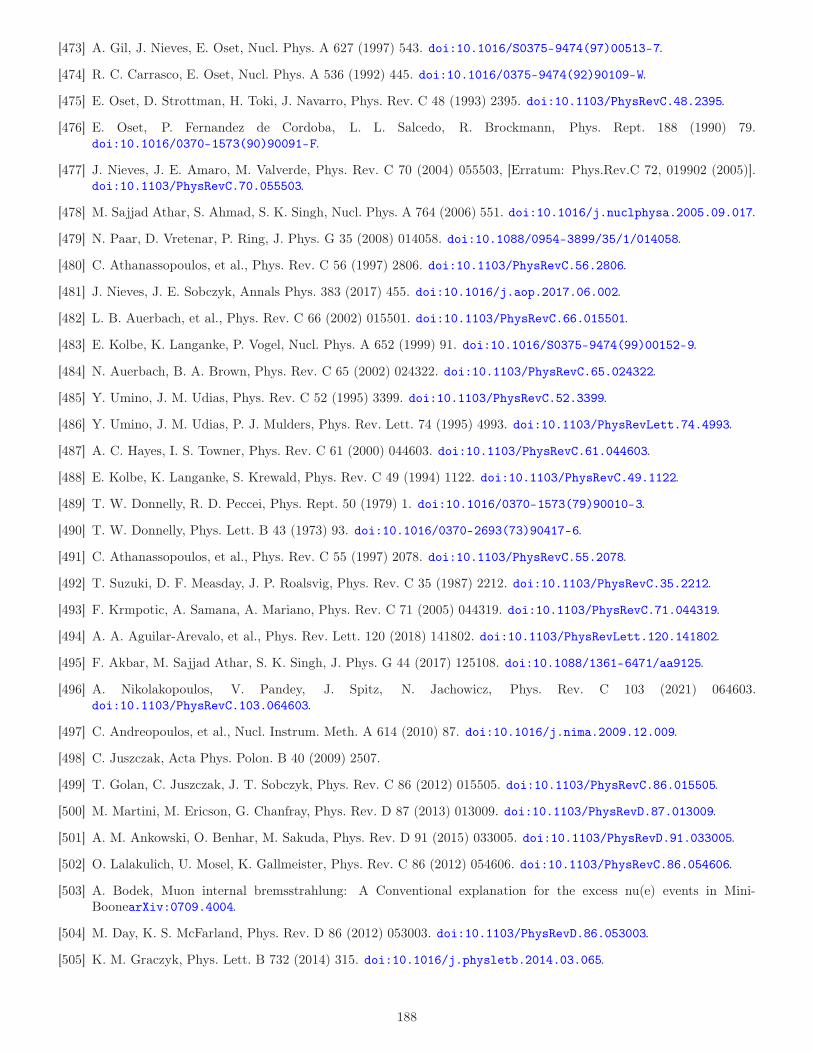
[473] A. Gil, J. Nieves, E. Oset, Nucl. Phys. A 627 (1997) 543. doi:10.1016/S0375-9474(97)00513-7.

[474] R. C. Carrasco, E. Oset, Nucl. Phys. A 536 (1992) 445. doi:10.1016/0375-9474(92)90109-W.

[475] E. Oset, D. Strottman, H. Toki, J. Navarro, Phys. Rev. C 48 (1993) 2395. doi:10.1103/PhysRevC.48.2395.

[476] E. Oset, P. Fernandez de Cordoba, L. L. Salcedo, R. Brockmann, Phys. Rept. 188 (1990) 79.doi:10.1016/0370-1573(90)90091-F.

[477] J. Nieves, J. E. Amaro, M. Valverde, Phys. Rev. C 70 (2004) 055503, [Erratum: Phys.Rev.C 72, 019902 (2005)].doi:10.1103/PhysRevC.70.055503.

[478] M. Sajjad Athar, S. Ahmad, S. K. Singh, Nucl. Phys. A 764 (2006) 551. doi:10.1016/j.nuclphysa.2005.09.017.

[479] N. Paar, D. Vretenar, P. Ring, J. Phys. G 35 (2008) 014058. doi:10.1088/0954-3899/35/1/014058.

[480] C. Athanassopoulos, et al., Phys. Rev. C 56 (1997) 2806. doi:10.1103/PhysRevC.56.2806.

[481] J. Nieves, J. E. Sobczyk, Annals Phys. 383 (2017) 455. doi:10.1016/j.aop.2017.06.002.

[482] L. B. Auerbach, et al., Phys. Rev. C 66 (2002) 015501. doi:10.1103/PhysRevC.66.015501.

[483] E. Kolbe, K. Langanke, P. Vogel, Nucl. Phys. A 652 (1999) 91. doi:10.1016/S0375-9474(99)00152-9.

[484] N. Auerbach, B. A. Brown, Phys. Rev. C 65 (2002) 024322. doi:10.1103/PhysRevC.65.024322.

[485] Y. Umino, J. M. Udias, Phys. Rev. C 52 (1995) 3399. doi:10.1103/PhysRevC.52.3399.

[486] Y. Umino, J. M. Udias, P. J. Mulders, Phys. Rev. Lett. 74 (1995) 4993. doi:10.1103/PhysRevLett.74.4993.

[487] A. C. Hayes, I. S. Towner, Phys. Rev. C 61 (2000) 044603. doi:10.1103/PhysRevC.61.044603.

[488] E. Kolbe, K. Langanke, S. Krewald, Phys. Rev. C 49 (1994) 1122. doi:10.1103/PhysRevC.49.1122.

[489] T. W. Donnelly, R. D. Peccei, Phys. Rept. 50 (1979) 1. doi:10.1016/0370-1573(79)90010-3.

[490] T. W. Donnelly, Phys. Lett. B 43 (1973) 93. doi:10.1016/0370-2693(73)90417-6.

[491] C. Athanassopoulos, et al., Phys. Rev. C 55 (1997) 2078. doi:10.1103/PhysRevC.55.2078.

[492] T. Suzuki, D. F. Measday, J. P. Roalsvig, Phys. Rev. C 35 (1987) 2212. doi:10.1103/PhysRevC.35.2212.

[493] F. Krmpotic, A. Samana, A. Mariano, Phys. Rev. C 71 (2005) 044319. doi:10.1103/PhysRevC.71.044319.

[494] A. A. Aguilar-Arevalo, et al., Phys. Rev. Lett. 120 (2018) 141802. doi:10.1103/PhysRevLett.120.141802.

[495] F. Akbar, M. Sajjad Athar, S. K. Singh, J. Phys. G 44 (2017) 125108. doi:10.1088/1361-6471/aa9125.

[496] A. Nikolakopoulos, V. Pandey, J. Spitz, N. Jachowicz, Phys. Rev. C 103 (2021) 064603.doi:10.1103/PhysRevC.103.064603.

[497] C. Andreopoulos, et al., Nucl. Instrum. Meth. A 614 (2010) 87. doi:10.1016/j.nima.2009.12.009.

[498] C. Juszczak, Acta Phys. Polon. B 40 (2009) 2507.

[499] T. Golan, C. Juszczak, J. T. Sobczyk, Phys. Rev. C 86 (2012) 015505. doi:10.1103/PhysRevC.86.015505.

[500] M. Martini, M. Ericson, G. Chanfray, Phys. Rev. D 87 (2013) 013009. doi:10.1103/PhysRevD.87.013009.

[501] A. M. Ankowski, O. Benhar, M. Sakuda, Phys. Rev. D 91 (2015) 033005. doi:10.1103/PhysRevD.91.033005.

[502] O. Lalakulich, U. Mosel, K. Gallmeister, Phys. Rev. C 86 (2012) 054606. doi:10.1103/PhysRevC.86.054606.

[503] A. Bodek, Muon internal bremsstrahlung: A Conventional explanation for the excess nu(e) events in Mini-BoonearXiv:0709.4004.

[504] M. Day, K. S. McFarland, Phys. Rev. D 86 (2012) 053003. doi:10.1103/PhysRevD.86.053003.

[505] K. M. Graczyk, Phys. Lett. B 732 (2014) 315. doi:10.1016/j.physletb.2014.03.065.

188

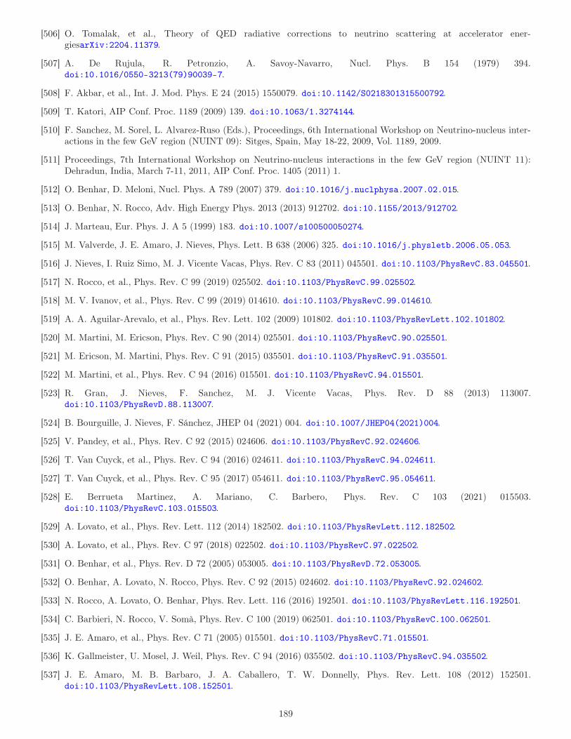
[506] O. Tomalak, et al., Theory of QED radiative corrections to neutrino scattering at accelerator ener-giesarXiv:2204.11379.

[507] A. De Rujula, R. Petronzio, A. Savoy-Navarro, Nucl. Phys. B 154 (1979) 394.doi:10.1016/0550-3213(79)90039-7.

[508] F. Akbar, et al., Int. J. Mod. Phys. E 24 (2015) 1550079. doi:10.1142/S0218301315500792.

[509] T. Katori, AIP Conf. Proc. 1189 (2009) 139. doi:10.1063/1.3274144.

[510] F. Sanchez, M. Sorel, L. Alvarez-Ruso (Eds.), Proceedings, 6th International Workshop on Neutrino-nucleus inter-actions in the few GeV region (NUINT 09): Sitges, Spain, May 18-22, 2009, Vol. 1189, 2009.

[511] Proceedings, 7th International Workshop on Neutrino-nucleus interactions in the few GeV region (NUINT 11):Dehradun, India, March 7-11, 2011, AIP Conf. Proc. 1405 (2011) 1.

[512] O. Benhar, D. Meloni, Nucl. Phys. A 789 (2007) 379. doi:10.1016/j.nuclphysa.2007.02.015.

[513] O. Benhar, N. Rocco, Adv. High Energy Phys. 2013 (2013) 912702. doi:10.1155/2013/912702.

[514] J. Marteau, Eur. Phys. J. A 5 (1999) 183. doi:10.1007/s100500050274.

[515] M. Valverde, J. E. Amaro, J. Nieves, Phys. Lett. B 638 (2006) 325. doi:10.1016/j.physletb.2006.05.053.

[516] J. Nieves, I. Ruiz Simo, M. J. Vicente Vacas, Phys. Rev. C 83 (2011) 045501. doi:10.1103/PhysRevC.83.045501.

[517] N. Rocco, et al., Phys. Rev. C 99 (2019) 025502. doi:10.1103/PhysRevC.99.025502.

[518] M. V. Ivanov, et al., Phys. Rev. C 99 (2019) 014610. doi:10.1103/PhysRevC.99.014610.

[519] A. A. Aguilar-Arevalo, et al., Phys. Rev. Lett. 102 (2009) 101802. doi:10.1103/PhysRevLett.102.101802.

[520] M. Martini, M. Ericson, Phys. Rev. C 90 (2014) 025501. doi:10.1103/PhysRevC.90.025501.

[521] M. Ericson, M. Martini, Phys. Rev. C 91 (2015) 035501. doi:10.1103/PhysRevC.91.035501.

[522] M. Martini, et al., Phys. Rev. C 94 (2016) 015501. doi:10.1103/PhysRevC.94.015501.

[523] R. Gran, J. Nieves, F. Sanchez, M. J. Vicente Vacas, Phys. Rev. D 88 (2013) 113007.doi:10.1103/PhysRevD.88.113007.

[524] B. Bourguille, J. Nieves, F. Sánchez, JHEP 04 (2021) 004. doi:10.1007/JHEP04(2021)004.

[525] V. Pandey, et al., Phys. Rev. C 92 (2015) 024606. doi:10.1103/PhysRevC.92.024606.

[526] T. Van Cuyck, et al., Phys. Rev. C 94 (2016) 024611. doi:10.1103/PhysRevC.94.024611.

[527] T. Van Cuyck, et al., Phys. Rev. C 95 (2017) 054611. doi:10.1103/PhysRevC.95.054611.

[528] E. Berrueta Martinez, A. Mariano, C. Barbero, Phys. Rev. C 103 (2021) 015503.doi:10.1103/PhysRevC.103.015503.

[529] A. Lovato, et al., Phys. Rev. Lett. 112 (2014) 182502. doi:10.1103/PhysRevLett.112.182502.

[530] A. Lovato, et al., Phys. Rev. C 97 (2018) 022502. doi:10.1103/PhysRevC.97.022502.

[531] O. Benhar, et al., Phys. Rev. D 72 (2005) 053005. doi:10.1103/PhysRevD.72.053005.

[532] O. Benhar, A. Lovato, N. Rocco, Phys. Rev. C 92 (2015) 024602. doi:10.1103/PhysRevC.92.024602.

[533] N. Rocco, A. Lovato, O. Benhar, Phys. Rev. Lett. 116 (2016) 192501. doi:10.1103/PhysRevLett.116.192501.

[534] C. Barbieri, N. Rocco, V. Somà, Phys. Rev. C 100 (2019) 062501. doi:10.1103/PhysRevC.100.062501.

[535] J. E. Amaro, et al., Phys. Rev. C 71 (2005) 015501. doi:10.1103/PhysRevC.71.015501.

[536] K. Gallmeister, U. Mosel, J. Weil, Phys. Rev. C 94 (2016) 035502. doi:10.1103/PhysRevC.94.035502.

[537] J. E. Amaro, M. B. Barbaro, J. A. Caballero, T. W. Donnelly, Phys. Rev. Lett. 108 (2012) 152501.doi:10.1103/PhysRevLett.108.152501.

189

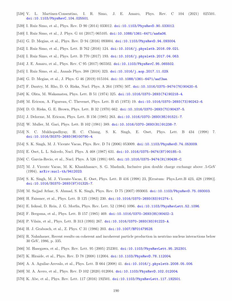
[538] V. L. Martinez-Consentino, I. R. Simo, J. E. Amaro, Phys. Rev. C 104 (2021) 025501.doi:10.1103/PhysRevC.104.025501.

[539] I. Ruiz Simo, et al., Phys. Rev. D 90 (2014) 033012. doi:10.1103/PhysRevD.90.033012.

[540] I. Ruiz Simo, et al., J. Phys. G 44 (2017) 065105. doi:10.1088/1361-6471/aa6a06.

[541] G. D. Megias, et al., Phys. Rev. D 94 (2016) 093004. doi:10.1103/PhysRevD.94.093004.

[542] I. Ruiz Simo, et al., Phys. Lett. B 762 (2016) 124. doi:10.1016/j.physletb.2016.09.021.

[543] I. Ruiz Simo, et al., Phys. Lett. B 770 (2017) 193. doi:10.1016/j.physletb.2017.04.063.

[544] J. E. Amaro, et al., Phys. Rev. C 95 (2017) 065502. doi:10.1103/PhysRevC.95.065502.

[545] I. Ruiz Simo, et al., Annals Phys. 388 (2018) 323. doi:10.1016/j.aop.2017.11.029.

[546] G. D. Megias, et al., J. Phys. G 46 (2019) 015104. doi:10.1088/1361-6471/aaf3ae.

[547] F. Dautry, M. Rho, D. O. Riska, Nucl. Phys. A 264 (1976) 507. doi:10.1016/0375-9474(76)90420-6.

[548] K. Ohta, M. Wakamatsu, Phys. Lett. B 51 (1974) 325. doi:10.1016/0370-2693(74)90218-4.

[549] M. Ericson, A. Figureau, C. Thevenet, Phys. Lett. B 45 (1973) 19. doi:10.1016/0370-2693(73)90242-6.

[550] D. O. Riska, G. E. Brown, Phys. Lett. B 32 (1970) 662. doi:10.1016/0370-2693(70)90437-5.

[551] J. Delorme, M. Ericson, Phys. Lett. B 156 (1985) 263. doi:10.1016/0370-2693(85)91521-7.

[552] W. Muller, M. Gari, Phys. Lett. B 102 (1981) 389. doi:10.1016/0370-2693(81)91238-7.

[553] N. C. Mukhopadhyay, H. C. Chiang, S. K. Singh, E. Oset, Phys. Lett. B 434 (1998) 7.doi:10.1016/S0370-2693(98)00790-4.

[554] S. K. Singh, M. J. Vicente Vacas, Phys. Rev. D 74 (2006) 053009. doi:10.1103/PhysRevD.74.053009.

[555] E. Oset, L. L. Salcedo, Nucl. Phys. A 468 (1987) 631. doi:10.1016/0375-9474(87)90185-0.

[556] C. Garcia-Recio, et al., Nucl. Phys. A 526 (1991) 685. doi:10.1016/0375-9474(91)90438-C.

[557] M. J. Vicente Vacas, M. K. Khankhasaev, S. G. Mashnik, Inclusive pion double charge exchange above .5-GeV(1994). arXiv:nucl-th/9412023.

[558] S. K. Singh, M. J. Vicente-Vacas, E. Oset, Phys. Lett. B 416 (1998) 23, [Erratum: Phys.Lett.B 423, 428 (1998)].doi:10.1016/S0370-2693(97)01325-7.

[559] M. Sajjad Athar, S. Ahmad, S. K. Singh, Phys. Rev. D 75 (2007) 093003. doi:10.1103/PhysRevD.75.093003.

[560] H. Faissner, et al., Phys. Lett. B 125 (1983) 230. doi:10.1016/0370-2693(83)91274-1.

[561] E. Isiksal, D. Rein, J. G. Morfin, Phys. Rev. Lett. 52 (1984) 1096. doi:10.1103/PhysRevLett.52.1096.

[562] F. Bergsma, et al., Phys. Lett. B 157 (1985) 469. doi:10.1016/0370-2693(85)90402-2.

[563] P. Vilain, et al., Phys. Lett. B 313 (1993) 267. doi:10.1016/0370-2693(93)91223-A.

[564] H. J. Grabosch, et al., Z. Phys. C 31 (1986) 203. doi:10.1007/BF01479528.

[565] R. Nahnhauer, Recent results on coherent and incoherent particle production in neutrino nucleus interactions below30 GeV, 1986, p. 335.

[566] M. Hasegawa, et al., Phys. Rev. Lett. 95 (2005) 252301. doi:10.1103/PhysRevLett.95.252301.

[567] K. Hiraide, et al., Phys. Rev. D 78 (2008) 112004. doi:10.1103/PhysRevD.78.112004.

[568] A. A. Aguilar-Arevalo, et al., Phys. Lett. B 664 (2008) 41. doi:10.1016/j.physletb.2008.05.006.

[569] M. A. Acero, et al., Phys. Rev. D 102 (2020) 012004. doi:10.1103/PhysRevD.102.012004.

[570] K. Abe, et al., Phys. Rev. Lett. 117 (2016) 192501. doi:10.1103/PhysRevLett.117.192501.

190

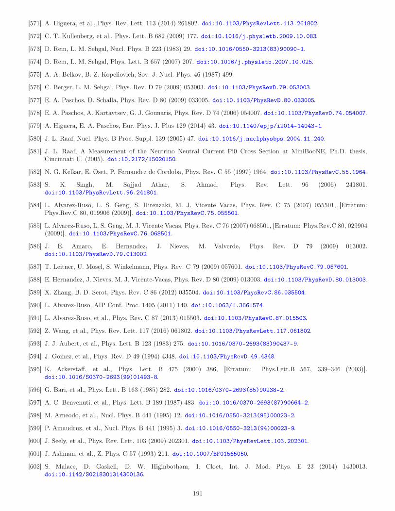
[571] A. Higuera, et al., Phys. Rev. Lett. 113 (2014) 261802. doi:10.1103/PhysRevLett.113.261802.

[572] C. T. Kullenberg, et al., Phys. Lett. B 682 (2009) 177. doi:10.1016/j.physletb.2009.10.083.

[573] D. Rein, L. M. Sehgal, Nucl. Phys. B 223 (1983) 29. doi:10.1016/0550-3213(83)90090-1.

[574] D. Rein, L. M. Sehgal, Phys. Lett. B 657 (2007) 207. doi:10.1016/j.physletb.2007.10.025.

[575] A. A. Belkov, B. Z. Kopeliovich, Sov. J. Nucl. Phys. 46 (1987) 499.

[576] C. Berger, L. M. Sehgal, Phys. Rev. D 79 (2009) 053003. doi:10.1103/PhysRevD.79.053003.

[577] E. A. Paschos, D. Schalla, Phys. Rev. D 80 (2009) 033005. doi:10.1103/PhysRevD.80.033005.

[578] E. A. Paschos, A. Kartavtsev, G. J. Gounaris, Phys. Rev. D 74 (2006) 054007. doi:10.1103/PhysRevD.74.054007.

[579] A. Higuera, E. A. Paschos, Eur. Phys. J. Plus 129 (2014) 43. doi:10.1140/epjp/i2014-14043-1.

[580] J. L. Raaf, Nucl. Phys. B Proc. Suppl. 139 (2005) 47. doi:10.1016/j.nuclphysbps.2004.11.240.

[581] J. L. Raaf, A Measurement of the Neutrino Neutral Current Pi0 Cross Section at MiniBooNE, Ph.D. thesis,Cincinnati U. (2005). doi:10.2172/15020150.

[582] N. G. Kelkar, E. Oset, P. Fernandez de Cordoba, Phys. Rev. C 55 (1997) 1964. doi:10.1103/PhysRevC.55.1964.

[583] S. K. Singh, M. Sajjad Athar, S. Ahmad, Phys. Rev. Lett. 96 (2006) 241801.doi:10.1103/PhysRevLett.96.241801.

[584] L. Alvarez-Ruso, L. S. Geng, S. Hirenzaki, M. J. Vicente Vacas, Phys. Rev. C 75 (2007) 055501, [Erratum:Phys.Rev.C 80, 019906 (2009)]. doi:10.1103/PhysRevC.75.055501.

[585] L. Alvarez-Ruso, L. S. Geng, M. J. Vicente Vacas, Phys. Rev. C 76 (2007) 068501, [Erratum: Phys.Rev.C 80, 029904(2009)]. doi:10.1103/PhysRevC.76.068501.

[586] J. E. Amaro, E. Hernandez, J. Nieves, M. Valverde, Phys. Rev. D 79 (2009) 013002.doi:10.1103/PhysRevD.79.013002.

[587] T. Leitner, U. Mosel, S. Winkelmann, Phys. Rev. C 79 (2009) 057601. doi:10.1103/PhysRevC.79.057601.

[588] E. Hernandez, J. Nieves, M. J. Vicente-Vacas, Phys. Rev. D 80 (2009) 013003. doi:10.1103/PhysRevD.80.013003.

[589] X. Zhang, B. D. Serot, Phys. Rev. C 86 (2012) 035504. doi:10.1103/PhysRevC.86.035504.

[590] L. Alvarez-Ruso, AIP Conf. Proc. 1405 (2011) 140. doi:10.1063/1.3661574.

[591] L. Alvarez-Ruso, et al., Phys. Rev. C 87 (2013) 015503. doi:10.1103/PhysRevC.87.015503.

[592] Z. Wang, et al., Phys. Rev. Lett. 117 (2016) 061802. doi:10.1103/PhysRevLett.117.061802.

[593] J. J. Aubert, et al., Phys. Lett. B 123 (1983) 275. doi:10.1016/0370-2693(83)90437-9.

[594] J. Gomez, et al., Phys. Rev. D 49 (1994) 4348. doi:10.1103/PhysRevD.49.4348.

[595] K. Ackerstaff, et al., Phys. Lett. B 475 (2000) 386, [Erratum: Phys.Lett.B 567, 339–346 (2003)].doi:10.1016/S0370-2693(99)01493-8.

[596] G. Bari, et al., Phys. Lett. B 163 (1985) 282. doi:10.1016/0370-2693(85)90238-2.

[597] A. C. Benvenuti, et al., Phys. Lett. B 189 (1987) 483. doi:10.1016/0370-2693(87)90664-2.

[598] M. Arneodo, et al., Nucl. Phys. B 441 (1995) 12. doi:10.1016/0550-3213(95)00023-2.

[599] P. Amaudruz, et al., Nucl. Phys. B 441 (1995) 3. doi:10.1016/0550-3213(94)00023-9.

[600] J. Seely, et al., Phys. Rev. Lett. 103 (2009) 202301. doi:10.1103/PhysRevLett.103.202301.

[601] J. Ashman, et al., Z. Phys. C 57 (1993) 211. doi:10.1007/BF01565050.

[602] S. Malace, D. Gaskell, D. W. Higinbotham, I. Cloet, Int. J. Mod. Phys. E 23 (2014) 1430013.doi:10.1142/S0218301314300136.

191

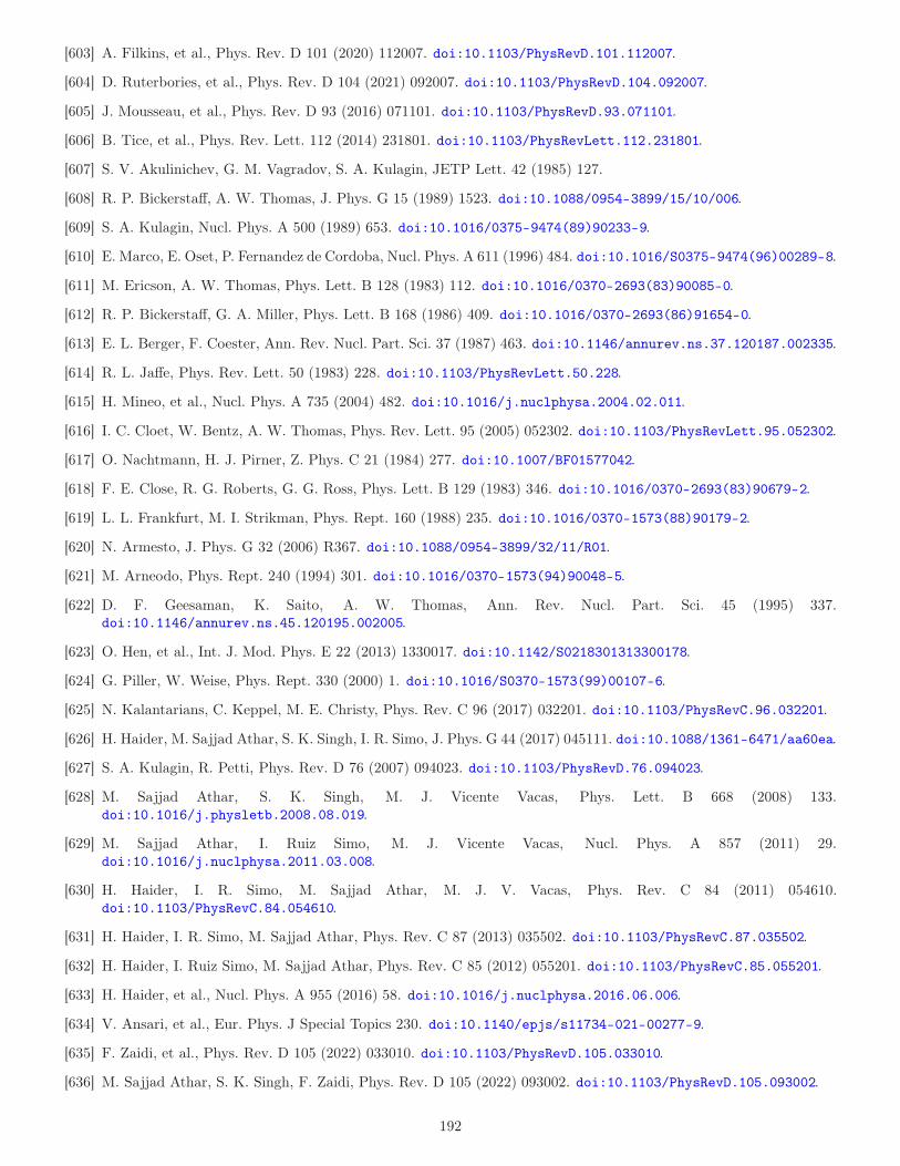
[603] A. Filkins, et al., Phys. Rev. D 101 (2020) 112007. doi:10.1103/PhysRevD.101.112007.

[604] D. Ruterbories, et al., Phys. Rev. D 104 (2021) 092007. doi:10.1103/PhysRevD.104.092007.

[605] J. Mousseau, et al., Phys. Rev. D 93 (2016) 071101. doi:10.1103/PhysRevD.93.071101.

[606] B. Tice, et al., Phys. Rev. Lett. 112 (2014) 231801. doi:10.1103/PhysRevLett.112.231801.

[607] S. V. Akulinichev, G. M. Vagradov, S. A. Kulagin, JETP Lett. 42 (1985) 127.

[608] R. P. Bickerstaff, A. W. Thomas, J. Phys. G 15 (1989) 1523. doi:10.1088/0954-3899/15/10/006.

[609] S. A. Kulagin, Nucl. Phys. A 500 (1989) 653. doi:10.1016/0375-9474(89)90233-9.

[610] E. Marco, E. Oset, P. Fernandez de Cordoba, Nucl. Phys. A 611 (1996) 484. doi:10.1016/S0375-9474(96)00289-8.

[611] M. Ericson, A. W. Thomas, Phys. Lett. B 128 (1983) 112. doi:10.1016/0370-2693(83)90085-0.

[612] R. P. Bickerstaff, G. A. Miller, Phys. Lett. B 168 (1986) 409. doi:10.1016/0370-2693(86)91654-0.

[613] E. L. Berger, F. Coester, Ann. Rev. Nucl. Part. Sci. 37 (1987) 463. doi:10.1146/annurev.ns.37.120187.002335.

[614] R. L. Jaffe, Phys. Rev. Lett. 50 (1983) 228. doi:10.1103/PhysRevLett.50.228.

[615] H. Mineo, et al., Nucl. Phys. A 735 (2004) 482. doi:10.1016/j.nuclphysa.2004.02.011.

[616] I. C. Cloet, W. Bentz, A. W. Thomas, Phys. Rev. Lett. 95 (2005) 052302. doi:10.1103/PhysRevLett.95.052302.

[617] O. Nachtmann, H. J. Pirner, Z. Phys. C 21 (1984) 277. doi:10.1007/BF01577042.

[618] F. E. Close, R. G. Roberts, G. G. Ross, Phys. Lett. B 129 (1983) 346. doi:10.1016/0370-2693(83)90679-2.

[619] L. L. Frankfurt, M. I. Strikman, Phys. Rept. 160 (1988) 235. doi:10.1016/0370-1573(88)90179-2.

[620] N. Armesto, J. Phys. G 32 (2006) R367. doi:10.1088/0954-3899/32/11/R01.

[621] M. Arneodo, Phys. Rept. 240 (1994) 301. doi:10.1016/0370-1573(94)90048-5.

[622] D. F. Geesaman, K. Saito, A. W. Thomas, Ann. Rev. Nucl. Part. Sci. 45 (1995) 337.doi:10.1146/annurev.ns.45.120195.002005.

[623] O. Hen, et al., Int. J. Mod. Phys. E 22 (2013) 1330017. doi:10.1142/S0218301313300178.

[624] G. Piller, W. Weise, Phys. Rept. 330 (2000) 1. doi:10.1016/S0370-1573(99)00107-6.

[625] N. Kalantarians, C. Keppel, M. E. Christy, Phys. Rev. C 96 (2017) 032201. doi:10.1103/PhysRevC.96.032201.

[626] H. Haider, M. Sajjad Athar, S. K. Singh, I. R. Simo, J. Phys. G 44 (2017) 045111. doi:10.1088/1361-6471/aa60ea.

[627] S. A. Kulagin, R. Petti, Phys. Rev. D 76 (2007) 094023. doi:10.1103/PhysRevD.76.094023.

[628] M. Sajjad Athar, S. K. Singh, M. J. Vicente Vacas, Phys. Lett. B 668 (2008) 133.doi:10.1016/j.physletb.2008.08.019.

[629] M. Sajjad Athar, I. Ruiz Simo, M. J. Vicente Vacas, Nucl. Phys. A 857 (2011) 29.doi:10.1016/j.nuclphysa.2011.03.008.

[630] H. Haider, I. R. Simo, M. Sajjad Athar, M. J. V. Vacas, Phys. Rev. C 84 (2011) 054610.doi:10.1103/PhysRevC.84.054610.

[631] H. Haider, I. R. Simo, M. Sajjad Athar, Phys. Rev. C 87 (2013) 035502. doi:10.1103/PhysRevC.87.035502.

[632] H. Haider, I. Ruiz Simo, M. Sajjad Athar, Phys. Rev. C 85 (2012) 055201. doi:10.1103/PhysRevC.85.055201.

[633] H. Haider, et al., Nucl. Phys. A 955 (2016) 58. doi:10.1016/j.nuclphysa.2016.06.006.

[634] V. Ansari, et al., Eur. Phys. J Special Topics 230. doi:10.1140/epjs/s11734-021-00277-9.

[635] F. Zaidi, et al., Phys. Rev. D 105 (2022) 033010. doi:10.1103/PhysRevD.105.033010.

[636] M. Sajjad Athar, S. K. Singh, F. Zaidi, Phys. Rev. D 105 (2022) 093002. doi:10.1103/PhysRevD.105.093002.

192

[637] P. Fernandez de Cordoba, E. Oset, Phys. Rev. C 46 (1992) 1697. doi:10.1103/PhysRevC.46.1697.

[638] E. Oset, A. Palanques-Mestre, Nucl. Phys. A 359 (1981) 289. doi:10.1016/0375-9474(81)90238-4.

[639] A. Gil, J. Nieves, E. Oset, Nucl. Phys. A 627 (1997) 599. doi:10.1016/S0375-9474(97)00515-0.

[640] C. Mahaux, P. F. Bortignon, R. A. Broglia, C. H. Dasso, Phys. Rept. 120 (1985) 1.doi:10.1016/0370-1573(85)90100-0.

[641] H. Haider, et al., Nucl. Phys. A 943 (2015) 58. doi:10.1016/j.nuclphysa.2015.08.008.

[642] S. A. Kulagin, R. Petti, Nucl. Phys. A 765 (2006) 126. doi:10.1016/j.nuclphysa.2005.10.011.

[643] C. H. Llewellyn Smith, Phys. Lett. B 128 (1983) 107. doi:10.1016/0370-2693(83)90084-9.

[644] J. S. Conway, et al., Phys. Rev. D 39 (1989) 92. doi:10.1103/PhysRevD.39.92.

[645] P. J. Sutton, A. D. Martin, R. G. Roberts, W. J. Stirling, Phys. Rev. D 45 (1992) 2349.doi:10.1103/PhysRevD.45.2349.

[646] K. Wijesooriya, P. E. Reimer, R. J. Holt, Phys. Rev. C 72 (2005) 065203. doi:10.1103/PhysRevC.72.065203.

[647] M. Gluck, E. Reya, A. Vogt, Z. Phys. C 53 (1992) 651. doi:10.1007/BF01559743.

[648] R. J. Glauber, ed. by W.E. Brittin and L.G. Dunham Interscience, New York.

[649] V. N. Gribov, Sov. Phys. JETP 29 (1969) 483.

[650] V. N. Gribov, Zh. Eksp. Teor. Fiz. 57 (1969) 1306.

[651] V. N. Gribov, Zh. Eksp. Teor. Fiz. 53 (1967) 654.

[652] V. A. Abramovsky, V. N. Gribov, O. V. Kancheli, Yad. Fiz. 18 (1973) 595.

[653] V. A. Karmanov, L. A. Kondratyuk, Pisma Zh. Eksp. Teor. Fiz. 18 (1973) 451.

[654] J. J. Sakurai, D. Schildknecht, Phys. Lett. B 40 (1972) 121. doi:10.1016/0370-2693(72)90300-0.

[655] J. D. Bjorken, Proc of the Int. Symp. on Electron and Photon Interactions at High energies, Cornell University(1971).

[656] A. Bramon, E. Etim, M. Greco, Phys. Lett. B 41 (1972) 609. doi:10.1016/0370-2693(72)90646-6.

[657] N. N. Nikolaev, B. G. Zakharov, Z. Phys. C 49 (1991) 607. doi:10.1007/BF01483577.

[658] A. H. Mueller, Nucl. Phys. B 415 (1994) 373. doi:10.1016/0550-3213(94)90116-3.

[659] N. Armesto, Eur. Phys. J. C 26 (2002) 35. doi:10.1007/s10052-002-1021-z.

[660] S. J. Brodsky, Acta Phys. Polon. B 36 (2005) 635.

[661] B. Z. Kopeliovich, J. G. Morfin, I. Schmidt, Prog. Part. Nucl. Phys. 68 (2013) 314.doi:10.1016/j.ppnp.2012.09.004.

[662] K. J. Eskola, V. J. Kolhinen, C. A. Salgado, Eur. Phys. J. C 9 (1999) 61. doi:10.1007/s100520050513.

[663] K. J. Eskola, V. J. Kolhinen, P. V. Ruuskanen, Nucl. Phys. B 535 (1998) 351.doi:10.1016/S0550-3213(98)00589-6.

[664] M. Hirai, S. Kumano, M. Miyama, Phys. Rev. D 64 (2001) 034003. doi:10.1103/PhysRevD.64.034003.

[665] M. Hirai, S. Kumano, T. H. Nagai, Phys. Rev. C 70 (2004) 044905. doi:10.1103/PhysRevC.70.044905.

[666] D. de Florian, R. Sassot, Phys. Rev. D 69 (2004) 074028. doi:10.1103/PhysRevD.69.074028.

[667] K. J. Eskola, V. J. Kolhinen, H. Paukkunen, C. A. Salgado, JHEP 05 (2007) 002.doi:10.1088/1126-6708/2007/05/002.

[668] M. Hirai, S. Kumano, T. H. Nagai, Phys. Rev. C 76 (2007) 065207. doi:10.1103/PhysRevC.76.065207.

[669] K. J. Eskola, H. Paukkunen, C. A. Salgado, JHEP 04 (2009) 065. doi:10.1088/1126-6708/2009/04/065.

193

[670] K. J. Eskola, P. Paakkinen, H. Paukkunen, C. A. Salgado, Eur. Phys. J. C 77 (2017) 163.doi:10.1140/epjc/s10052-017-4725-9.

[671] I. Schienbein, et al., Phys. Rev. D 80 (2009) 094004. doi:10.1103/PhysRevD.80.094004.

[672] T. Stavreva, et al., JHEP 01 (2011) 152. doi:10.1007/JHEP01(2011)152.

[673] K. Kovarik, et al., Phys. Rev. Lett. 106 (2011) 122301. doi:10.1103/PhysRevLett.106.122301.

[674] D. de Florian, R. Sassot, P. Zurita, M. Stratmann, Phys. Rev. D 85 (2012) 074028.doi:10.1103/PhysRevD.85.074028.

[675] I. Helenius, M. Walt, W. Vogelsang, TUJU21: NNLO nuclear parton distribution functions with electroweak-bosonproduction data from the LHC (2021). arXiv:2112.11904.

[676] H. Khanpour, et al., Phys. Rev. D 104 (2021) 034010. doi:10.1103/PhysRevD.104.034010.

[677] R. Abdul Khalek, J. J. Ethier, J. Rojo, G. van Weelden, JHEP 09 (2020) 183. doi:10.1007/JHEP09(2020)183.

[678] K. J. Eskola, Nucl. Phys. A 910-911 (2013) 163. doi:10.1016/j.nuclphysa.2012.12.029.

[679] K. Kovarik, et al., Phys. Rev. D 93 (2016) 085037. doi:10.1103/PhysRevD.93.085037.

[680] J. F. Owens, et al., Phys. Rev. D 75 (2007) 054030. doi:10.1103/PhysRevD.75.054030.

[681] J. Pumplin, et al., JHEP 07 (2002) 012. doi:10.1088/1126-6708/2002/07/012.

[682] D. Stump, et al., JHEP 10 (2003) 046. doi:10.1088/1126-6708/2003/10/046.

[683] S. A. Kulagin, R. Petti, Nucl. Phys. B Proc. Suppl. 159 (2006) 180. doi:10.1016/j.nuclphysbps.2006.08.036.

[684] K. F. Muzakka, et al., Compatibility of Neutrino DIS Data and Its Impact on Nuclear Parton Distribution Functions(2022). arXiv:2204.13157.

[685] V. Mamyan, Measurements of F2 and R=σL/σT on Nuclear Targets in the Nucleon Resonance Re-gionarXiv:1202.1457.

[686] J. J. Aubert, et al., Nucl. Phys. B 272 (1986) 158. doi:10.1016/0550-3213(86)90346-9.

[687] L. W. Whitlow, Deep Inelastic Structure Functions From Electron Scattering on Hydrogen, Deuterium, and Ironat 0.6-GeV2 ≤ Q2 ≤ 30-GeV2, Master’s thesis (1990).

[688] S. Dasu, et al., Phys. Rev. D 49 (1994) 5641. doi:10.1103/PhysRevD.49.5641.

[689] I. C. Cloet, W. Bentz, A. W. Thomas, Phys. Lett. B 642 (2006) 210. doi:10.1016/j.physletb.2006.08.076.

[690] I. Schienbein, et al., Phys. Rev. D 77 (2008) 054013. doi:10.1103/PhysRevD.77.054013.

[691] E. D. Bloom, F. J. Gilman, Phys. Rev. Lett. 25 (1970) 1140. doi:10.1103/PhysRevLett.25.1140.

[692] E. D. Bloom, F. J. Gilman, Phys. Rev. D 4 (1971) 2901. doi:10.1103/PhysRevD.4.2901.

[693] S. P. Malace, et al., Phys. Rev. C 80 (2009) 035207. doi:10.1103/PhysRevC.80.035207.

[694] I. Niculescu, et al., Phys. Rev. Lett. 85 (2000) 1186. doi:10.1103/PhysRevLett.85.1186.

[695] W. Melnitchouk, R. Ent, C. Keppel, Phys. Rept. 406 (2005) 127. doi:10.1016/j.physrep.2004.10.004.

[696] O. Lalakulich, et al., AIP Conf. Proc. 1189 (2009) 276. doi:10.1063/1.3274170.

[697] D. Wang, et al., Phys. Rev. Lett. 111 (2013) 082501. doi:10.1103/PhysRevLett.111.082501.

[698] O. Lalakulich, W. Melnitchouk, E. A. Paschos, Phys. Rev. C 75 (2007) 015202. doi:10.1103/PhysRevC.75.015202.

[699] F. Gross, S. Liuti, Phys. Rev. C 45 (1992) 1374. doi:10.1103/PhysRevC.45.1374.

[700] F. E. Close, W. Melnitchouk, Phys. Rev. C 68 (2003) 035210. doi:10.1103/PhysRevC.68.035210.

[701] H. Gallagher, Nucl. Phys. B Proc. Suppl. 112 (2002) 188. doi:10.1016/S0920-5632(02)01775-9.

[702] A. Rubbia, 1st workshop on neutrino- nucleus interactions in few gev region (nuint01) (2001).

194

[703] Y. Hayato, L. Pickering, Eur. Phys. J. ST 230 (2021) 4469. doi:10.1140/epjs/s11734-021-00287-7.

[704] Y. Hayato, Acta Phys. Polon. B 40 (2009) 2477.

[705] F. Cavanna, O. Palamara, Nucl. Phys. B Proc. Suppl. 112 (2002) 183. doi:10.1016/S0920-5632(02)01767-X.

[706] G. Battistoni, et al., A neutrino-nucleon interaction generator for the FLUKA Monte Carlo code, 2009.

[707] J. Nieves, F. Sanchez, I. Ruiz Simo, M. J. Vicente Vacas, Phys. Rev. D 85 (2012) 113008.doi:10.1103/PhysRevD.85.113008.

[708] J. E. Amaro, et al., Eur. Phys. J. ST 230 (2021) 4321. doi:10.1140/epjs/s11734-021-00289-5.

[709] O. Benhar, A. Fabrocini, S. Fantoni, I. Sick, Nucl. Phys. A 579 (1994) 493. doi:10.1016/0375-9474(94)90920-2.

[710] K. M. Graczyk, J. T. Sobczyk, Phys. Rev. D 77 (2008) 053001, [Erratum: Phys.Rev.D 79, 079903 (2009)].doi:10.1103/PhysRevD.79.079903.

[711] A. Bodek, U. K. Yang, AIP Conf. Proc. 670 (1) (2003) 110. doi:10.1063/1.1594324.

[712] O. Buss, et al., Phys. Rept. 512 (2012) 1. doi:10.1016/j.physrep.2011.12.001.

[713] P. A. Rodrigues, et al., Phys. Rev. Lett. 116 (2016) 071802, [Addendum: Phys.Rev.Lett. 121, 209902 (2018)].doi:10.1103/PhysRevLett.116.071802.

[714] P. Abratenko, et al., Phys. Rev. Lett. 128 (2022) 151801. doi:10.1103/PhysRevLett.128.151801.

[715] P. Abratenko, et al., Phys. Rev. D 105 (2022) 072001. doi:10.1103/PhysRevD.105.072001.

[716] U. Mosel, J. Phys. G 46 (2019) 113001. doi:10.1088/1361-6471/ab3830.

[717] K. Abe, et al., Phys. Rev. D 101 (2020) 112004. doi:10.1103/PhysRevD.101.112004.

[718] R. Acciarri, et al., Phys. Rev. D 98 (2018) 052002. doi:10.1103/PhysRevD.98.052002.

[719] T. Golan, J. T. Sobczyk, J. Zmuda, Nucl. Phys. B Proc. Suppl. 229 (2012) 499.doi:10.1016/j.nuclphysbps.2012.09.136.

195

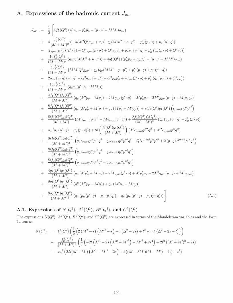
A. Expressions of the hadronic current Jµν

Jµν =1

2

[

4f21 (Q

2)(

p′µpν + p′νpµ − (p · p′ −MM ′)gµν)

+ 4f22 (Q

2)

(M +M ′)2(

−MM ′Q2gµν + qµ (−qν(MM ′ + p · p′) + p′ν (p · q) + pν (p′ · q))

− 2gµν (p · q) (p′ · q)−Q2gµν (p · p′) +Q2pµp′ν + pµqν (p

′ · q) + p′µ(

qν (p · q) +Q2pν))

+16f2

3 (Q2)

(M +M ′)2(qµqν(MM ′ + p · p′)) + 4g21(Q

2)(

(p′µpν + pµp′ν)− (p · p′ +MM ′)gµν

)

+4g22(Q

2)

(M +M ′)2(

MM ′Q2gµν + qµ (qν(MM ′ − p · p′) + p′ν (p · q) + pν (p′ · q))

− 2gµν (p · q) (p′ · q)−Q2gµν (p · p′) +Q2pµp′β + pµqν (p

′ · q) + p′µ(

qν (p · q) +Q2pν))

+16g23(Q

2)

(M +M ′)2(qµqν(p

′ · p−MM ′))

+4f1(Q

2)f2(Q2)

(M +M ′)

(

qµ (M′pν −Mp′ν) + 2Mgµν (p

′ · q)−Mp′µqν − 2M ′gµν (p · q) +M ′pµqν)

+8f1(Q

2)f3(Q2)

(M +M ′)

(

qµ (Mp′ν +M ′pν) + qν(

Mp′µ +M ′pµ))

+ 8if1(Q2)g1(Q

2)(

ǫµναβ pαp′

δ)

+8if1(Q

2)g2(Q2)

(M +M ′)

(

M ′ǫµναβpαqβ −Mǫµναβp

′αqβ)

+8f2(Q

2)f3(Q2)

(M +M ′)2(

qν(

pµ (p′ · q)− p′µ (p · q)

)

+ qµ (pν (p′ · q)− p′ν (p · q))) + 8i

(

f2(Q2)g1(Q

2)

(M +M ′)

)

(

Mǫµναβp′αqβ +M ′ǫµναβp

αqβ)

+8if2(Q

2)g2(Q2)

(M +M ′)2

(

qµǫναβδpαp′

βqδ − qνǫµαβδpαp′βqδ −Q2ǫµναβpαp′

β+ 2 (p · q) ǫµναβp′αqβ

)

+8if2(Q

2)g3(Q2)

(M +M ′)2

(

qµǫναβδpαp′

βqδ − qνǫµαβδpαp′βqδ

)

+8if3(Q

2)g2(Q2)

(M +M ′)2

(

qµǫναβδpαp′

βqδ − qνǫµαβδpαp′βqδ

)

+4g1(Q

2)g2(Q2)

(M +M ′)

(

qµ (Mp′ν +M ′pν)− 2Mgµν (p′ · q) +Mp′µqν − 2M ′gµν (p · q) +M ′pµqν

)

+8g1(Q

2)g3(Q2)

(M +M ′)

(

qµ (M ′pν −Mp′ν) + qν(

M ′pµ −Mp′µ))

+8g2(Q

2)g3(Q2)

(M +M ′)2(

qν(

pµ (p′ · q)− p′µ (p · q)

)

+ qµ (pν (p′ · q)− p′ν (p · q))

)

]

. (A.1)

A.1. Expressions of N(Q2), Ah(Q2), Bh(Q2), and Ch(Q2)

The expressions N(Q2), Ah(Q2), Bh(Q2), and Ch(Q2) are expressed in terms of the Mandelstam variables and the formfactors as:

N(Q2) = f21 (Q

2)

(

1

2

(

2(

M2 − s)

(

M ′2 − s)

− t(

∆2 − 2s)

+ t2 +m2l

(

∆2 − 2s− t)

)

)

+f22 (Q

2)

(M +M ′)2

(

1

4

(

−2t(

M4 − 2s(

M2 +M ′2)

+M ′4 + 2s2)

+ 2t2(

(M +M ′)2 − 2s)

+ m2l

(

2∆(M +M ′)(

M2 +M ′2 − 2s)

+ t(

(M − 3M ′)(M +M ′) + 4s) + t2)

196

+ m4l (−((3M −M ′)(M +M ′) + t))

))

+ g21(Q2)

(

1

2

(

2(

M2 − s)

(

M ′2 − s)

− t(

(M +M ′)2 − 2s)

+ t2 +m2l

(

(M +M ′)2 − 2s− t)

)

)

+|g2(Q2)|2(M +M ′)2

(

1

4

(

4(

∆2 − t)

(

(

M2 − s)

(

M ′2 − s)

+ st)

+m2l

(

4∆(

M3 +M2M ′ −M(3s+ t) +M ′s)

+ 2∆2(

(M +M ′)2 − 2s− t)

− (4s+ t)(

∆2 − t))

+ 2∆2(

−2(

M2 − s)

(

M ′2 − s)

− t(

(M +M ′)2 + 2s)

+ t2)

+ m4l

(

∆2 + 4M∆− t))

)

+g23(Q

2)

(M +M ′)2(

m2l

(

m2l − t

) (

∆2 − t))

+f1(Q

2)f2(Q2)

(M +M ′)

(

−(

t(M +M ′)(

∆2 − t)

+m2l

(

−∆(

M ′2 − s)

+M ′t)

+m4lM))

± f1(Q2)g1(Q

2)(

−(

t(

M2 +M ′2 − 2s− t)

+m2l

(

M2 −M ′2 + t)))

± Re[f1(Q2)g2(Q

2)]

(M +M ′)

(

−∆(

t(

M2 +M ′2 − 2s− t)

+m2l

(

M2 −M ′2 + t)))

± f2(Q2)g1(Q

2)

(M +M ′)

(

−(M +M ′)(

t(

M2 +M ′2 − 2s− t)

+m2l

(

M2 −M ′2 + t)))

± Re[f2(Q2)g2(Q

2)]

(M +M ′)2

(

∆(−(M +M ′))(

t(

M2 +M ′2 − 2s− t)

+m2l

(

M2 −M ′2 + t)))

+Re[g1(Q

2)g2(Q2)]

(M +M ′)

((

∆(

−t(M +M ′)2 + t2)

+m2l

(

M3 +M2M ′ +∆(

(M +M ′)2 − 2s− t)

− 3Ms−Mt+M ′s) +m4lM )) +

g1(Q2)g3(Q

2)

(M +M ′)

(

−2m2l

(

m2lM +M3 −M2M ′ −M(s+ t) +M ′s

))

+Re[g2(Q

2)g3(Q2)]

(M +M ′)2(

m2l

(

−2∆(

m2lM +M3 −M2M ′ −M(s+ t) +M ′s

)

−(

∆2 − t) (

m2l + 2M2 − 2s− t

)))

(A.2)

where (+)− sign represents the (anti)neutrino induced scattering and the Mandelstam variables are defined as,

s =M2 + 2ME, t =M2 +M ′2 − 2ME′, (A.3)

with ∆ =M ′ −M .

Ah(Q2) = −2[

f21 (Q

2)

(

±1

2(M +M ′)

(

∆2 − t)

)

± f22 (Q

2)

(M +M ′)2

(

1

2t(M +M ′)

(

∆2 − t)

)

± g21(Q2)

(

1

2∆(

(M +M ′)2 − t)

)

± |g2(Q2)|2(M +M ′)2

(

1

2t∆(

(M +M ′)2 − t)

)

± f1(Q2)f2(Q

2)

(M +M ′)

(

1

2

(

4MM ′t+ t2 −∆2 (M +M ′)2)

)

+ f1(Q2)g1(Q

2)(

−M ′(

M2 +M ′2 − 2s− t))

+Re[f1(Q

2)g2(Q2)]

(M +M ′)

(

1

2

((

M2 +M ′2 − 2s− t)

(

−t− 2M ′∆+∆2)

+m2l

(

∆2 − t)

)

)

+f1(Q

2)g3(Q2)

(M +M ′)

(

−m2l

(

∆2 − t))

+f2(Q

2)g1(Q2)

(M +M ′)

(

1

2

((

M2 −M ′2 − t)(

M2 +M ′2 − 2s− t)

+ m2l

(

(M +M ′)2 − t)))

+Re[f2(Q

2)g2(Q2)]

(M +M ′)2

(

1

2

(

(M +M ′)(

∆2 − t)

(

m2l +M2 +M ′2 − 2s− t

)

+ ∆(

m2l

(

(M +M ′)2 − t)

+(

M2 −M ′2 − t)(

M2 +M ′2 − 2s− t)))

)

+f2(Q

2)g3(Q2)

(M +M ′)2(

−m2l (M +M ′)

(

∆2 − t))

± Re[g1(Q2)g2(Q

2)]

(M +M ′)

(

1

2

(

(M +M ′)2 − t)

(−∆2 − t))

]

(A.4)

Bh(Q2) =2

M ′

[

f21 (Q

2)

(

±1

4

(

t(

∆2 − 2s)

− t2 − 2M ′∆(

M2 − s)

+m2l

(

M2 + 2MM ′ −M ′2 + t))

)

± f22 (Q

2)

(M +M ′)2

(

1

4

(

t(M +M ′)(

M3 +M2M ′ −M(

M ′2 + 2s+ t)

+M ′3 −M ′t)

197

+ m2l

(

M4 + t(M +M ′)2 −M ′4))

)

± g21(Q2)

(

1

4((

−2M ′(M +M ′)(

M2 − s)

+ t(

(M +M ′)2 − 2s)

− t2 +m2l

(

M2 − 2MM ′ −M ′2 + t)))

± |g2(Q2)|2(M +M ′)2

(

1

4∆(

2M ′(

−2m2lM

2 −M4 +M2(

M ′2 + s+ t)

+ s(

t−M ′2))

+∆(

−2M ′(M +M ′)(

M2 − s)

+ t(

(M +M ′)2 − 2s)

− t2)

+m2l

(

M2 − 2MM ′ −M ′2 + t)))

± f1(Q2)f2(Q

2)

(M +M ′)

(

1

2

(

M4M ′ +M3t−M2M ′(

M ′2 + s)

−Mt(

M ′2 + 2s+ t)

+M ′(

M ′2 − t)

(s+ t)

+ m2l

(

M3 +M2M ′ +M(

M ′2 + t)

−M ′3 +M ′t)))

+ f1(Q2)g1(Q

2)

(

1

2

(

t(

M2 +M ′2 − 2s)

− 2s(

s−M2)

− t2

− m2l

(

M2 +M ′2 − 2s− t)))

+Re[f1(Q

2)g2(Q2)]

(M +M ′)

(

−1

2

(

M4M ′ − 2M3s+M2(

M ′3 −M ′(s+ t)−∆(2s+ t))

+ 2Ms(s+ t)−M ′3s−M ′2∆t+M ′st+ 2∆s2 + 2∆st+∆t2 +m2l

(

M3 +M2∆−M(3s+ t) + ∆(

M ′2 − 2s− t))

+ m4lM))

+f1(Q

2)g3(Q2)

(M +M ′)

(

m2lM

(

m2l +M2 − s− t

))

+f2(Q

2)g1(Q2)

(M +M ′)

(

1

2

(

−M ′ (M2 − s)

(

M2 +M ′2 − 2s)

+ t(

M3 + 2M2M ′ +MM ′2 +M ′3 − 3M ′s)

− t2(M +M ′)−m2l

(

M2M ′ +M(

M ′2 + s)

+M ′(

M ′2 − 2s− t))

+ m4lM))

+Re[f2(Q

2)g2(Q2)]

(M +M ′)2

(

1

4

(

2(

M3(

−M ′3 +M ′(3s+ t) + ∆t)

+M2(

M ′4 −M ′3∆−M ′2(3s+ t)

+ M ′∆(3s+ 2t) + 2st) +MM ′s(

M ′2 − 2s− 3t)

+ s(

M ′2 − t)(

2(s+ t)−M ′2)

+M∆t(

M ′2 − t)

+ M ′∆(s+ t)(

M ′2 − 2s− t))

+m2l

(

−2M4 − 2M3M ′ +M2(−2M ′∆+ 2s+ t)− 2M∆(

M ′2 + s)

+ 2MM ′(3s+ t)

+ 2M ′∆(

−M ′2 + 2s+ t)

−(

M ′2 − t)

(4s+ t))

−m4l

(

3M2 −M ′2 + t))

)

+f2(Q

2)g3(Q2)

(M +M ′)2

(

1

2m2

l

(

m2l

(

M2 + 2MM ′ −M ′2 + t)

− 2M ′∆(

M2 − s)

+ t(

∆2 − 2s)

− t2)

)

± Re[g1(Q2)g2(Q

2)]

(M +M ′)

(

1

2

(

M ′(

−2m2lM

2 −M4 +M2(

M ′2 + s+ t)

+ s(

t−M ′2))

+ ∆(

m2l

(

M2 − 2MM ′ −M ′2 + t)

− 2M ′(M +M ′)(

M2 − s)

+ t(

(M +M ′)2 − 2s)

− t2))) ]

(A.5)

Ch(Q2) = 2

±Im[f1(Q2)g2(Q

2)]

(M +M ′)

(

−t+ 2M∆+∆2)

± Im[f2(Q2)g2(Q

2)]

(M +M ′)

−t+∆(

M2 −M ′2 + t)

M +M ′ +∆2

+Im[g1(Q

2)g2(Q2)]

(M +M ′)

(

M2 +M ′2 − 2s− t+m2l

)

+Im[g3(Q

2)g2(Q2)]

(M +M ′)2(

2m2l∆)

]

(A.6)

A.2. Expressions of Al(Q2), Bl(Q2) and C l(Q2)

The expressions Al(Q2), Bl(Q2) and Cl(Q2) are expressed in terms of the Mandelstam variables and the form factors as:

Al(Q2) = 2

[

f21 (Q

2)

(

1

2ml

(

M2 + 2MM ′ − s)

)

+f22 (Q

2)

(M +M ′)2

(

1

4ml

(

−m2l ((3M −M ′)(M +M ′) + t)− 2M4 + 2M2

(

M ′2 + s)

+ 4MM ′t

− 2(

M ′2 − t)

(s+ t)))

+ g21(Q2)

(

1

2ml

(

M2 − 2MM ′ − s)

)

+|g2(Q2)|2(M +M ′)2

(

1

4ml

(

(

∆2 − t)

(

m2l + 4M2 + 2M ′2 − 2s− 2t

)

+ 2∆(

2m2lM − 4M2∆

+ 3M(

M ′2 − s− t)

+M ′(

−M ′2 + s+ t))

+ 2∆2(

M2 − 2MM ′ − s)

)

)

198

+g23(Q

2)

(M +M ′)2(

m3l

(

∆2 − t))

+f1(Q

2)f2(Q2)

(M +M ′)

(

−1

2ml

(

2m2lM −∆

(

2M2 −M ′2 − s)

− t(3M +M ′))

)

+ f1(Q2)g1(Q

2)(

−ml

(

M2 − s))

+Re[f1(Q

2)g2(Q2)]

(M +M ′)

(

−ml∆(

M2 − s))

+f2(Q

2)g1(Q2)

(M +M ′)

(

−ml(M +M ′)(

M2 − s))

+Re[f2(Q

2)g2(Q2)]

(M +M ′)2(

−ml∆(M +M ′)(

M2 − s))

+Re[g1(Q

2)g2(Q2)]

(M +M ′)

(

1

2ml

(

2m2lM + 4M3 + 2M2(∆− 2M ′) +MM ′(3M ′ − 4∆)

− 3M(s+ t)−M ′3 +M ′(s+ t)− 2∆s))

+g1(Q

2)g3(Q2)

(M +M ′)

(

−(

2m3lM −ml∆

(

M ′2 − s− t)))

+Re[g3(Q

2)g2(Q2)]

(M +M ′)2

(

−ml

(

m2l

(

∆2 + 2M∆− t)

− t(M ′2 − s− t))) ]

(A.7)

Bl(Q2) =2

M ′

[

f21 (Q

2)

(

1

4mlM ′(

m2l

(

−(

M2 + 2MM ′ −M ′2 + t))

+ 2(

M2 − s)

(

M ′2 − s)

− t∆2 + 2st+ t2)

)

+f22 (Q

2)

(M +M ′)2

(

1

8mlM ′ (m4

l ((3M −M ′)(M +M ′) + t) +m2l

(

∆2 − t) (

2(M +M ′)2 + t)

− 2t(

M4 − 2s(

M2 +M ′2)

+M ′4 + 2s2)

+ 2t2(

(M +M ′)2 − 2s)

))

+ g21(Q2)

(

1

4mlM ′(

m2l

(

−(

M2 − 2MM ′ −M ′2 + t))

+ 2(

M2 − s)

(

M ′2 − s)

− t(M +M ′)2 + 2st+ t2)

)

+|g2(Q2)|2(M +M ′)2

(

1

8mlM ′(

m4l

(

−(

∆2 + 4M∆− t))

+m2l

(

−2∆2(

M2 − 2MM ′ −M ′2 + t)

−(

4M2 − t) (

∆2 − t)

+ 4M∆(2M∆+ t))

+ 2∆2(

2(

M2 − s)

(

M ′2 − s)

− t(M +M ′)2 + 2st+ t2)

− 8∆2(

(

M2 − s)

(

M ′2 − s)

+ st)

+ 4(

∆2 − t)

(

(

M2 − s)

(

M ′2 − s)

+ st)))

+g23(Q

2)

(M +M ′)2

(

−1

2mlM

′ (m2l − t

) (

∆2 − t)

)

+f1(Q

2)f2(Q2)

(M +M ′)

(

1

2mlM ′ (m2

l − t) (

m2lM + (M +M ′)

(

(M −M ′)2 − t))

)

+ f1(Q2)g1(Q

2)

(

1

2mlM ′ (m2

l − t)

(

M2 +M ′2 − 2s− t)

)

+Re[f1(Q

2)g2(Q2)]

(M +M ′)

(

1

2mlM ′∆

(

m2l − t

)

(

M2 +M ′2 − 2s− t)

)

+f2(Q

2)g1(Q2)

(M +M ′)

(

1

2mlM ′ (m2

l − t)

(M +M ′)(

M2 +M ′2 − 2s− t)

)

+Re[f2(Q

2)g2(Q2)]

(M +M ′)2

(

1

2mlM ′∆

(

m2l − t

)

(M +M ′)(

M2 +M ′2 − 2s− t)

)

+Re[g1(Q

2)g2(Q2)]

(M +M ′)

(

1

2mlM ′(

−m4lM +m2

l

(

−2M3 +M2(2M ′ −∆) +M(2M ′∆+ t) + ∆(

M ′2 − t))

+ ∆(

2(

M2 − s)

(

M ′2 − s)

− t(

(M +M ′)2 − 2s)

+ t2)

− 2∆(

(

M2 − s)

(

M ′2 − s)

+ st))

)

+g1(Q

2)g3(Q2)

(M +M ′)

(

mlMM ′ (m2l − t

))

+Re[g2(Q

2)g3(Q2)]

(M +M ′)2

(

1

2mlM

′ (m2l − t

) (

∆2 + 2M∆− t)

)

]

(A.8)

Cl(Q2) = 2

[

Im[g1(Q2)g2(Q

2)]

(M +M ′)(ml(M +M ′)) +

Im[g3(Q2)g2(Q

2)]

(M +M ′)2(2mlt)

]

(A.9)

B. Cabibbo theory, SU(3) symmetry and weak N −Y transition form factors

In the Cabibbo theory, the weak vector and the axial-vector currents corresponding to the ∆S = 0 and ∆S = 1hadronic currents whose matrix elements are defined between the states |N〉 and |N ′〉 are assumed to belong to the octet

199

representation of SU(3). Accordingly, they are defined as:

V µi = qFiγ

µq, Aµi = qFiγ

µγ5q, (B.1)

where Fi =λi

2 (i = 1− 8) are the generators of flavor SU(3) and λis are the well known Gell-Mann matrices.From the property of SU(3) group, it follows that there are three corresponding SU(2) subgroups of SU(3) which

must be invariant under the interchange of quark pairs ud, ds and us respectively, if the group is invariant under theinterchange of u, d and s quarks. Each of these SU(2) subgroups has raising and lowering operators. One of them isSU(2)I , generated by the generators (λ1, λ2, λ3) to be identified with the isospin operators (I1, I2, I3) in the isospin space.For example, I± of isospin is given by

I± = I1 ± iI2 = F1 ± iF2 =1

2(λ1 ± iλ2). (B.2)

The other two are defined as SU(2)U and SU(2)V generated by the generators (λ6, λ7,12 (√3λ8−λ3)) and (λ4, λ5,

12 (√3λ8+

λ3)), respectively, in U-spin and V-spin space with (d s) and (u s) forming the basic doublet representation of SU(2)Uand SU(2)V . For more details, see Ref. [10].

From the Gell-Mann matrices λi, one may obtain the raising and lowering operators with U-spin and V-spin in analogywith I-spin as:

U± = U1 ± iU2 = F6 ± iF7, V± = V1 ± iV2 = F4 ± iF5.

In neutron β-decay, the vector and the axial-vector currents for this transition can be written as

ψuγµψd = qγµ

(

λ1 + iλ22

)

q = V 1+i2µ , ψuγµγ5ψd = qγµγ5

(

λ1 + iλ22

)

q = A1+i2µ .

Similarly, s→ u and u→ s transformations are written as

ψuγµψs = qγµ

(

λ4 + iλ52

)

q = V 4+i5µ , ψsγµψu = qγµ

(

λ4 − iλ52

)

q = V 4−i5µ , (B.3)

ψuγµγ5ψs = qγµγ5

(

λ4 + iλ52

)

q = A4+i5µ , ψsγµγ5ψu = qγµγ5

(

λ4 − iλ52

)

q = A4−i5µ . (B.4)

The electromagnetic current which is vector current is written using the SU(3) content of the charge operator e = I3+Y2 =

λ3 +1

2√3λ8 as:

Jemµ = V 3

µ +1√3V 8µ . (B.5)

Therefore, the charge changing weak vector and axial-vector currents are written, in Cabibbo theory, as:

V ±µ =

[

V 1µ ± iV 2

µ

]

cos θc +[

V 4µ ± iV 5

µ

]

sin θc,

A±µ =

[

A1µ ± iA2

µ

]

cos θc +[

A4µ ± iA5

µ

]

sin θc. (B.6)

In the Cabibbo theory, the isovector part of the electromagnetic current Jµem i.e. V 3

µ along with the weak vector currentsV µ± are assumed to transform as an octet of vector currents under SU(3). Similarly, the axial vector currents are also

assumed to transform as an octet under SU(3). The weak transition form factors fi(q2) and gi(q

2); i = 1 − 3 aredetermined using Cabibbo theory of V −A interaction extended to the strange sector.

In general, the expression for the matrix element of the transition between the two states of baryons (say Bi and Bk),through the SU(3) octet (Vj or Aj) of currents can be written as:

< Bi|Vj |Bk >= ifijkFV + dijkD

V , < Bi|Aj |Bk >= ifijkFA + dijkD

A. (B.7)

FV and DV are determined from the experimental data on the electromagnetic form factors, and FA and DA aredetermined from the experimental data on the semileptonic decays of neutron and hyperons. The physical baryon octetstates are written in terms of their octet state Bi as discussed in Section 3.3.1. The matrix element of electromagneticcurrents between proton, and neutron states are obtained as

〈p|Jem|p〉 = DV

3+ FV , 〈n|Jem|n〉 =

1

2

[

−2

3DV − 2

3DV

]

= −2DV

3. (B.8)

The nucleon electromagnetic form factors can be written in terms of their SU(3) coupling constants as

200

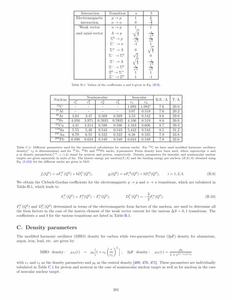
Interaction Transition a bElectromagnetic p→ p 1 1

3interaction n→ n 0 - 23

Weak vector n→ p 1 1

and axial-vector Λ→ p -√

32 - 1√

6

Σ0 → p - 1√2

1√2

Σ− → n -1 1

Σ± → Λ 0√

23

Σ− → Σ0√2 0

Ξ− → Λ√

32 - 1√

6

Ξ− → Σ0 1√2

1√2

Ξ0 → Σ+ 1 1Ξ− → Ξ0 1 -1

Table B.1: Values of the coefficients a and b given in Eq. (B.9).

NucleusNonisoscalar Isoscalar

B.E./A T/Acn1 cp1 cn2 cp2 c1 c2

12C - - - - 1.692 1.082∗ 7.6 20.027Al - - - - 3.07 0.519 7.6 20.240Ar 3.64 3.47 0.569 0.569 3.53 0.542 8.6 29.056Fe 4.050 3.971 0.5935 0.5935 4.106 0.519 8.8 30.063Cu 4.31 4.214 0.586 0.586 4.163 0.606 8.7 29.3118Sn 5.55 5.40 0.543 0.543 5.442 0.543 8.5 31.2197Au 6.79 6.55 0.522 0.522 6.38 0.535 7.9 33.8208Pb 6.890 6.624 0.549 0.549 6.624 0.549 7.8 32.6

Table C.1: Different parameters used for the numerical calculations for various nuclei. For 12C we have used modified harmonic oscillatordensity(∗ c2 is dimensionless) and for 40Ar, 56Fe and 208Pb nuclei, 2-parameter Fermi density have been used, where superscript n andp in density parameters(cn,p

i ; i=1,2) stand for neutron and proton, respectively. Density parameters for isoscalar and nonisoscalar nucleartargets are given separately in units of fm. The kinetic energy per nucleon(T/A) and the binding energy per nucleon (B.E/A) obtained usingEq. (5.153) for the different nuclei are given in MeV.

fi(Q2) = aFV

i (Q2) + bDVi (Q

2), gi(Q2) = aFA

i (Q2) + bDAi (Q

2), i = 1, 2, 3. (B.9)

We obtain the Clebsch-Gordan coefficients for the electromagnetic p→ p and n→ n transitions, which are tabulated inTable-B.1, which leads to

FVi (Q2) = F p

i (Q2)− Fn

i (Q2), DV

i (Q2) = −3

2Fni (Q

2). (B.10)

FVi (Q2) and DV

i (Q2) determined in terms of the electromagnetic form factors of the nucleon, are used to determine allthe form factors in the case of the matrix element of the weak vector current for the various ∆S = 0, 1 transitions. Thecoefficients a and b for the various transitions are listed in Table-B.1.

C. Density parameters

The modified harmonic oscillator (MHO) density for carbon while two-parameter Fermi (2pF) density for aluminium,argon, iron, lead, etc. are given by:

MHO density : ρN (r) = ρ0

[

1 + c2

(

r

c1

)2]

, 2pF density : ρN (r) =ρ0

1 + e(r−c1)/c2

with c1 and c2 as the density parameters and ρ0 as the central density [469, 470, 471]. These parameters are individuallytabulated in Table C.1 for proton and neutron in the case of nonisoscalar nuclear target as well as for nucleon in the caseof isoscalar nuclear target.

201