etudes des proprietes des neutrinos dans les contextes
TRANSCRIPT
HAL Id: tel-00450051https://tel.archives-ouvertes.fr/tel-00450051
Submitted on 25 Jan 2010
HAL is a multi-disciplinary open accessarchive for the deposit and dissemination of sci-entific research documents, whether they are pub-lished or not. The documents may come fromteaching and research institutions in France orabroad, or from public or private research centers.
L’archive ouverte pluridisciplinaire HAL, estdestinée au dépôt et à la diffusion de documentsscientifiques de niveau recherche, publiés ou non,émanant des établissements d’enseignement et derecherche français ou étrangers, des laboratoirespublics ou privés.
Etudes des proprietes des neutrinos dans les contextesastrophysique et cosmologique
J. Gava
To cite this version:J. Gava. Etudes des proprietes des neutrinos dans les contextes astrophysique et cosmologique.Physique Nucléaire Théorique [nucl-th]. Université Paris Sud - Paris XI, 2009. Français. tel-00450051
THESE de DOCTORATde l’UNIVERSITE PARIS XI
Specialite :
Physique Theorique
presentee par :
Jerome Gava
pour obtenir le grade deDOCTEUR de l’UNIVERSITE PARIS XI ORSAY
Sujet de la these :
Etudes des proprietes des neutrinosdans les contextes astrophysique
et cosmologique
soutenue publiquement le 26 juin 2009, devant le jury compose de :
Mme C. Volpe Directrice de theseMme A. Abada President du jury
Mme S. Davidson RapporteurM. G. Sigl Rapporteur
M. A. B. Balantekin ExaminateurM. M. Mezzetto Examinateur
REMERCIEMENTS
Ce travail a pu etre effectue grace a une allocation de recherche obtenue parl’Ecole doctorale 381 ainsi qu’a un monitorat a l’universite de Paris 7.Je suis reconnaissant a Dominique Guillemaud-Mueller ainsi qu’ a Bernard Berthierde m’avoir accueilli a la division de recherche de l’IPN d’Orsay.Je remercie Cristina Volpe de m’avoir pris dans son groupe, d’avoir dirige mesrecherches, et de m’avoir propose un sujet passionant, a la croisee de plusieursdomaines et en plein essor. Je veux lui exprimer toute ma gratitude pour leclimat d’amicale et stimulante collaboration qui s’est etabli entre nous. Je luisuis reconnaissant pour son investissement afin que ma these se passe dans lesmeilleures conditions possibles; j’ai aussi apprecie les discussions de physique etautres que nous avons eues, son oreille attentive a mes problemes de physique etautres, sa disponibilite totale et sa motivation dans ce projet que nous avons sumener jusqu’au bout.I thank all the members of my PhD committee for accepting to be part of it. Ideeply thank Gunter Sigl and Sacha Davidson for accepting to be referee of myPhD manuscript and for their comments. I am grateful to Baha Balantekin andMauro Mezzetto for accepting to be in my PhD committee and for their com-ments. Je suis reconnaissant a double titre envers Asma Abada qui a bien accepted’etre presidente de mon jury mais egalement qui m’a oriente bien heureusementvers Cristina lorsque je cherchais un sujet de these.Grace au financement CNRS obtenu par Cristina, j’ai pu me rendre plusieursfois dans le groupe NPAC de physique a l’universite de Madison. Je remercie lesmembres du groupe pour leur accueil et particulierement A. Baha Balantekin,Yamac Pehlivan ainsi que Joao Henrique De Jesus.J’ai eu l’occasion de travailler a plusieurs reprises au laboratoire d’Astro-particuleset Cosmologie (APC) a Paris 7. Je remercie Julien Serreau, Alessandra Tonazzoainsi que Michela Marafini. Je tiens a remercier bien evidemment Bachir Mousal-lam le responsable du groupe de physique theorique de l’IPN, tous les membresdu groupe de physique pour leur accueil et leur gentillesse ainsi que la secretairedu groupe, Nathalie Escoubeirou. Je suis reconnaissant en particulier a MarcellaGrasso pour avoir organise mon seminaire au labo, et a Samuel Friot pour m’avoirdonne des conseils pour les calculs a boucles (et pour les restaurants etoiles). Lepresent travail a necessite de nombreux calculs numeriques, je remercie le serviceinformatique de l’IPN et en particulier Paul Gara qui m’a aide a surmonter lesproblemes numeriques dus a l’interaction neutrino-neutrino notamment.J’exprime ma gratitude envers mes collegues de bureau avec qui j’ai partage ces
3 annees. Merci a Xavier Barillier-Pertuisel, Emilie Passemar, Rabia Yekken,Jean-Paul Ebran, Anthea Fantina, ainsi que Sebastien Galais. Je n’oublie pas deremercier les differents post docs que j’ai croise sur ma route et qui m’ont bienaide a apprehender le domaine; Merci donc a Rimantas Lazauskas, Julien Welzelet Jim Kneller. J’ai une pensee particuliere pour mon ami Charles-ChristopheJean-Louis avec qui j’ai pu faire un article en plus des travaux que j’ai effectuesdurant ma these. Je repense sans regret aux nombreux week-end ensoleilles passesa calculer des diagrammes a une boucle, aux seances de muscu a parler de Super-Symetrie. Je suis heureux d’avoir pu mener ce projet avec lui jusqu’au boutmalgre les difficultes rencontrees.Je suis aussi reconnaissant envers mes amis pour leurs encouragements et soutiensdans ce travail. Merci a Maxime Besset, Antoine Deleglise, Clement Millotte, etHicham Quasmi. Merci a mes parents et a ma soeur, pour leurs encouragementset soutiens indefectibles. Last but not least, mes remerciements vont a Agathepour les moments de bonheur que nous avons partages depuis mon DEA dephysique theorique, au Japon ou en France, ensemble ou lorsque nous etions auxantipodes.

A mes parents,
Someday you will find me,caught beneath the landslidein a champagne supernova in the sky.Champagne Supernova, Oasis.
Contents
I Neutrino Physics: present status and open questions 1
II General introduction 7
1 Neutrino Oscillations: the theoretical framework 91.1 The oscillation phenomenon . . . . . . . . . . . . . . . . . . . . . 9
1.1.1 2 flavors in vacuum. . . . . . . . . . . . . . . . . . . . . . 101.1.2 3 flavors in vacuum . . . . . . . . . . . . . . . . . . . . . . 131.1.3 CP-violation in vacuum . . . . . . . . . . . . . . . . . . . 14
1.2 Oscillations in matter . . . . . . . . . . . . . . . . . . . . . . . . . 151.2.1 The Mikheyev-Smirnov-Wolfenstein (MSW) effect . . . . . 201.2.2 3 flavours in matter . . . . . . . . . . . . . . . . . . . . . . 23
2 Neutrino oscillations: the experimental results and perspectives 312.1 The solar data: θ12 and ∆m2
21 . . . . . . . . . . . . . . . . . . . . 312.1.1 The Standard Solar Model (SSM) . . . . . . . . . . . . . . 312.1.2 The radiochemical detector experiments . . . . . . . . . . 332.1.3 The Cherenkov detector experiments. . . . . . . . . . . . . 342.1.4 The solar neutrino problem . . . . . . . . . . . . . . . . . 35
2.2 The atmospheric data: θ23 and ∆m223 . . . . . . . . . . . . . . . . 38
2.2.1 The atmospheric neutrino anomaly . . . . . . . . . . . . . 382.2.2 Long-baseline accelerator experiments . . . . . . . . . . . . 42
2.3 The unknown third mixing angle: θ13 . . . . . . . . . . . . . . . . 432.3.1 Upper bound for θ13 . . . . . . . . . . . . . . . . . . . . . 43
2.4 The hierarchy problem . . . . . . . . . . . . . . . . . . . . . . . . 432.4.1 What about ∆m2
31 ? . . . . . . . . . . . . . . . . . . . . . 442.5 Current and future neutrino experiments . . . . . . . . . . . . . . 44
2.5.1 Current and near-future experiments . . . . . . . . . . . . 452.5.2 Future long-term experiments . . . . . . . . . . . . . . . . 46
3 Neutrinos and core-collapse supernovae 513.1 General description of core-collapse supernovae . . . . . . . . . . . 52
3.1.1 A qualitative picture . . . . . . . . . . . . . . . . . . . . . 52
i
3.1.2 The neutrino fluxes and the neutrino spheres . . . . . . . . 55
3.2 Our supernova model . . . . . . . . . . . . . . . . . . . . . . . . . 58
3.2.1 The density profile . . . . . . . . . . . . . . . . . . . . . . 58
3.2.2 The neutrino fluxes at the neutrino spheres . . . . . . . . . 59
3.2.3 R-process nucleosynthesis . . . . . . . . . . . . . . . . . . 60
III Neutrino properties and supernovae 65
4 CP-violation and supernova neutrinos 67
4.1 CP effects with neutrino interactions at tree level . . . . . . . . . 68
4.1.1 Exact analytical formulas . . . . . . . . . . . . . . . . . . 68
4.1.2 Numerical results . . . . . . . . . . . . . . . . . . . . . . . 74
4.2 CP effects including one loop corrections . . . . . . . . . . . . . . 79
4.2.1 Theoretical framework . . . . . . . . . . . . . . . . . . . . 79
4.2.2 Explicit CP-violation phase dependence . . . . . . . . . . 85
5 Neutrino-neutrino interactions 89
5.1 Theoretical framework . . . . . . . . . . . . . . . . . . . . . . . . 89
5.1.1 The effective interaction Hamiltonian . . . . . . . . . . . . 89
5.1.2 The Neutrino Bulb Model . . . . . . . . . . . . . . . . . . 91
5.2 The different collective behaviours . . . . . . . . . . . . . . . . . . 95
5.2.1 The synchronized regime . . . . . . . . . . . . . . . . . . . 96
5.2.2 The bipolar regime . . . . . . . . . . . . . . . . . . . . . . 98
5.2.3 The spectral splits . . . . . . . . . . . . . . . . . . . . . . 104
5.2.4 Phenomenological implications on the fluxes . . . . . . . . 108
6 Collective neutrino oscillations in supernovae and CP-violation111
6.1 Analytical results . . . . . . . . . . . . . . . . . . . . . . . . . . . 111
6.2 General condition for CP-violation in supernovae . . . . . . . . . 114
6.3 Numerical results . . . . . . . . . . . . . . . . . . . . . . . . . . . 115
7 A dynamical collective calculation of supernova neutrino signals121
7.1 Introduction . . . . . . . . . . . . . . . . . . . . . . . . . . . . . . 121
7.1.1 A dynamic supernova density profile . . . . . . . . . . . . 121
7.1.2 Multiple resonances and phase effects . . . . . . . . . . . . 123
7.2 A signature for small θ13 in inverted hierarchy . . . . . . . . . . . 126
7.2.1 Signal on Earth . . . . . . . . . . . . . . . . . . . . . . . . 128
7.2.2 Conclusions . . . . . . . . . . . . . . . . . . . . . . . . . . 131
ii
IV Leptonic CP-violation in the early Universe 133
8 CP-violation effects on the neutrino degeneracy parameter 1358.1 Introduction . . . . . . . . . . . . . . . . . . . . . . . . . . . . . . 135
8.1.1 The neutrino degeneracy parameter and implications . . . 1358.1.2 The neutron to proton ratio . . . . . . . . . . . . . . . . . 137
8.2 Neutrino flavor oscillations in the early universe . . . . . . . . . . 1398.2.1 Theoretical framework . . . . . . . . . . . . . . . . . . . . 1398.2.2 The comoving variables . . . . . . . . . . . . . . . . . . . . 142
8.3 CP-violation: an analytical result . . . . . . . . . . . . . . . . . . 1438.4 Numerical results . . . . . . . . . . . . . . . . . . . . . . . . . . . 144
V Conclusion 145
VI Appendix 151
A The MNSP matrix and its parametrization 153A.1 The Dirac neutrino case . . . . . . . . . . . . . . . . . . . . . . . 153A.2 The parametrization of the MNSP matrix . . . . . . . . . . . . . 154A.3 The Majorana case . . . . . . . . . . . . . . . . . . . . . . . . . . 157
B The adiabaticity notion 159B.1 An analytic approximate formula . . . . . . . . . . . . . . . . . . 159B.2 The adiabaticity parameter . . . . . . . . . . . . . . . . . . . . . 162B.3 The Landau-Zener formula . . . . . . . . . . . . . . . . . . . . . . 163
C Several possible formalisms for the neutrino evolution equations167C.1 The Schrodinger equation for wave functions . . . . . . . . . . . . 167C.2 The Schrodinger equation for evolution operators . . . . . . . . . 168C.3 The Liouville-Von Neumann equation: the density matrix formalism169C.4 The polarization vector formalism . . . . . . . . . . . . . . . . . . 172C.5 Equivalences among the formalisms . . . . . . . . . . . . . . . . . 173
D Some details concerning the neutrino-neutrino calculations 175D.1 The differential number density of neutrinos . . . . . . . . . . . . 175D.2 The rotating frame . . . . . . . . . . . . . . . . . . . . . . . . . . 178D.3 The corotating frame and the adiabaticity . . . . . . . . . . . . . 179
iii
Part I
Neutrino Physics: present statusand open questions
1

Neutrinos are extraordinary particles, as they play a pivotal role in the mod-ern physics, from nuclear physics to physics beyond the Standard Model, andfrom astrophysics to cosmology. Let us briefly remind the milestones in the dis-covery of neutrinos of different flavours as well as of the oscillation phenomenon.
Neutrinos were first born theoretically when Pauli proposed the existence ofa light (but massive) electrically neutral particle of spin half to solve the prob-lem of the observed continuous spectra of electrons produced in nuclear β-decay.In 1933, Fermi writing his theory of weak interaction, named this particle theneutrino (little neutron) since the neutron was discovered by Chadwick one yearbefore. In 1942 Wang first proposed to use neutrino capture to detect neutrinosexperimentally. Its experimental discovery was made by Cowan and Reines in1956 who used the Savannah River nuclear reactor as a source of neutrinos shotinto protons producing neutrons and positrons both of which could be detected.It finally turned out that both the proposed and the observed particles were ac-tually antineutrinos. In 1962 Lederman, Schwartz and Steinberger brought theindication of the doublet structure of the leptons through the discovery of themuon neutrino. The first detection of tau neutrinos was announced in the summerof 2000 by the DONUT collaboration at Fermilab, making it the latest particleof the Standard Model to have been directly observed. The existence of a familyof three neutrinos had already been inferred by both theoretical consistency andexperimental data from LEP from Z0 decay. The Standard Model of particlespredict that the neutrino is massless and consequently cannot change its flavour.
In the same time, other crucial properties of neutrinos were being proposedand investigated like the phenomenon of neutrino oscillation. It was first pro-posed by Pontecorvo in 1957, using an analogy with the neutral kaon system,who predicted an oscillation of neutrinos to antineutrinos. Only afterwards, de-veloping his theory, he finally thought of oscillations between flavours.
The theories of thermonuclear reactions made in the 20’s and 30’s, turnedout to explain the production of energy by the stars like our Sun. Gamow andSchoenberg in the 40’s made the hypothesis that core-collapse supernovae couldproduce a huge emission of neutrinos. After the observation of neutrinos it be-came clear that stars were powerful neutrino sources and could give preciousinformation on neutrino properties and on star evolution as well.
Starting in the late 1960s, R. Davis pioneering experiment measured solarneutrinos for the first time and found that the number of electron neutrinos ar-riving from the sun was between one third and one half the number predictedby the Standard Solar Model, a discrepancy which became known as the solarneutrino problem. Another neutrino problem showed up when people decidedto measure the atmospheric neutrinos created by reactions of cosmic rays on theatmosphere, since it was an important background in the proton decay search.It turned out that the underground neutrino observatories measured an anomalyin the atmospheric fluxes. One of the proposals to solve simultaneously the solarneutrino problem and the atmospheric anomaly was to consider that neutrinos
3
are massive particles, and therefore oscillate which means that while travelingthey can change their flavour.
Super-Kamiokande first brought the crucial discovery of neutrino oscillationin 1998 by measuring a νµ deficit for up-going atmospheric neutrinos compared todown going ones in the detector. This was the first experimental proof of physicsbeyond the Standard Model. In 2000, the experimental results of SNO were thefirst to clearly indicate that the total flux of neutrinos detected by neutral currentinteractions was compatible with the standard solar models. Finding a smaller νe
flux than expected meant that some of them have oscillated into another flavour.Wolfenstein in 1978, then Mikheyev and Smirnov in 1986 proposed a mech-
anism for neutrinos to undergo a resonant flavour conversion in their oscillationwhile propagating through matter (which became to be known as the MSW ef-fect). It was Bethe who showed that an adiabatic conversion might occur in theSun and be at the origin of the solar neutrino deficit. In 2002 Kamland identifiedthe large mixing angle solution to the solar neutrino deficit problem giving thefirst experimental evidence that the MSW effect occurs in the Sun.
The discovery of neutrino oscillation has an enormous impact in various do-mains of physics. In particular it implies that the neutrino interaction and massbasis are not identical and are related by a mixing matrix. This matrix wasproposed in 1962 by Maki, Nakagawa, and Sakata who supposed 3 flavour familyof neutrinos. This matrix may be complex and in addition to three mixing an-gles, it possesses a complex term containing the CP-violating phase. Importantquestions remain open, such as the neutrino nature (Majorana versus Dirac),the value of θ13, the hierarchy problem, and the possible existence of CP viola-tion in the lepton sector. In particular the CP-violation can help explaining thematter-antimatter asymmetry in the Universe, one of the fundamental questionsin cosmology.
In 1987, Kamiokande, IMB and Baksan detected for the first time neutrinoscoming from a supernova explosion near our galaxy. The observation of solarand 1987A neutrinos opened the era of neutrino astronomy. This event, prov-ing that core-collapse supernovae are producing neutrinos, has already furnishedconstraints about particle physics, and given information on neutrinos and onthe supernova explosion mechanism. Several problems still remain concerningsupernovae. We do not have a perfectly clear picture of the explosion mecha-nism, and the precise astrophysical conditions under which the heavy elementsare produced still remain unknown.
The aim of this thesis is to investigate the neutrino properties using astro-physical and cosmological contexts. CP-violation in the lepton sector is a crucialissue which depending on the value of the third mixing angle, might require verylong term accelerator facilities. We explore for the first time the possibility to usesupernova neutrinos to learn about the Dirac phase either from direct effects ina observatory or from indirect effects in the star. We first study the influence ofthe CP-violating phase in the neutrino propagation inside the supernova within
4
the MSW framework. We establish with exact analytical formulas under whichconditions there might be CP effects in supernova. We then explore its conse-quences on the neutrino fluxes, the electron fraction which is a key element inthe r-process for the heavy elements nucleosynthesis. We also observe the effectsof such a phase on the neutrino events that could be detected on Earth. Suchnumerical calculations have required the development of numerical codes in 3flavours to describe neutrino propagation in matter. In a second work, we addedthe neutrino-neutrino interaction, and investigated the validity of the analyticalformula found in the previous work, we also modify our existing code to includethis non-linear interaction and study the consequences on the CP effects. Re-cent developments in the past three years have shown that its inclusion deeplychanges our comprehension of neutrino propagation in matter and engenders newcollective phenomena. In the third work, we have studied an even more realisticcase by including a dynamical density of matter inside the star. The presence ofa shock wave, created during the rebound of the collapsing matter on the proto-neutron core of the star, in addition with the neutrino-neutrino interaction caninduce particular effects on the neutrino propagation, and can let a characteristicimprint on the neutrino fluxes on Earth depending on the neutrino hierarchy andon the third mixing angle. In a final work we explore the consequence of theCP-violating phase on the neutrino degeneracy parameter, in the early Universeenvironment, before Big Bang Nucleosynthesis (BBN) and neutrino decoupling.
The thesis is structured as follows. The first chapter gives the theoreticalframework for neutrino oscillations. The second chapter presents historically themain experiments performed as well as those to come and the results they broughtin neutrino physics. The third chapter introduces the core-collapse supernovaemodel we use. The fourth chapter tackles the impact of including a CP-violatingphase in the neutrino propagation in a supernova and the implications on themain observables. Because of the recent and impressive developments, we give adescription of the neutrino-neutrino interaction and the change it implies for theneutrino propagation in a supernova environment. The following chapter showsthe effect of CP-violation when the neutrino self-interaction is included. Thesixth chapter uses an even more realistic description of the supernova media byadding a dynamic density profile and investigate the consequences on a neutrinoflux on Earth. The seventh chapter studies the effect of the CP-violating phasebefore BBN. The last chapter is the conclusion.
5

6

Part II
General introduction
7

Chapter 1
Neutrino Oscillations: thetheoretical framework
The idea of neutrino oscillation was first proposed by Pontecorvo in 1957 [96, 97],a couple of years after Gell-Mann and Pais pointed out the interesting conse-
quences which follow from the fact that K0 and K0
are not identical particles.
The possible K0 → K0
transition, which is due to the weak interactions, leads tothe necessity of considering neutral K-mesons as a superposition of two particlesK0
1 and K02 . Pontecorvo envisaged oscillations between other neutral particles
and thought of ν → ν oscillations and consequently of the leptonic neutrinocharge. He developed this conjecture in the subsequent years (predicted thatthe neutrino associated with the muon may be different from the one relatedto the electron) till 1967 where the oscillation hypothesis was given the modernform [98]. Assuming that neutrinos are capable of oscillating means that neutri-nos are massive particles and therefore implies that the Standard Model is flawed.
1.1 The oscillation phenomenon
Considering a two-level quantum system with fixed energies Ei, the associatedevolution equation is :
id
dt
(
Ψ1
Ψ2
)
=
(
E1 00 E2
)(
Ψ1
Ψ2
)
. (1.1)
If the system is in one of its eigenstates |Ψi〉 (which therefore are stationarystates), solving the Schrodinger equation will obviously yield : |Ψi(t)〉 = e−iEit|Ψi(0)〉.If, however, the initial state is not one of the eigenstates of the system, the prob-ability to find the system in this state will oscillate in time with the frequencyω21 = E2 − E1.
9
The case of neutrinos
Neutrinos are produced by the charged-current weak interactions and thereforeare weak-eigenstates. νe, νµ or ντ are different from the states that diagonalizethe neutrino mass matrix because of the oscillation phenomenon. To link themass states to the flavour states, one requires a unitary matrix U called the lep-ton mixing matrix, or Maki-Nakagawa-Sakata-Pontecorvo (MNSP) matrix1 [87](leptonic analog of the quark mixing matrix, the Cabibbo-Kobayashi-Maskawa(CKM) matrix). It relates a neutrino flavour eigenstate |να〉 produced or ab-sorbed alongside with the corresponding charged lepton, to the mass eigenstates|νi〉:
|να〉 = U∗αi |νi〉 , (1.2)
Following the previous general argument, if the initial state at t = 0 is |ν(0)〉 =|να〉 = U∗
αj |νj〉 where the α (j) subscript corresponds respectively to the flavour(mass) eigenstate; the neutrino state at a later time t is then
|ν(t)〉 = U∗αj e
−iEjt|νj〉 . (1.3)
The probability amplitude of finding the neutrino at the time t in a flavour state|νβ〉 is
A(να → νβ; t) = 〈νβ|ν(t)〉 = U∗αj e
−iEjt 〈νβ|νj〉 = UβiU∗αj e
−iEjt 〈νi|νj〉 = Uβj e−iEjt U∗
αj .(1.4)
As usual, the sum over all intermediate states j is implied. The factor U∗αj = U †
jα
represent the transition amplitude of the initial flavour neutrino eigenstate να
into a mass eigenstate νj; the factor e−iEjt is just the phase acquired during thetime evolution of the mass eigenstate νj with energy Ej , and finally the factorUβj converts the time-evolved mass eigenstate νj into the flavour eigenstate νβ.The neutrino oscillation probability, i.e. the transformation probability of aflavour neutrino eigenstate να into another one νβ, is then
P (να → νβ ; t) = |A(να → νβ; t)|2 = |Uβj e−iEjt U∗
αj |2 . (1.5)
To analyze in detail the neutrino oscillation phenomenon, let us first focus on thesimple case where only two neutrino species νe and νµ are involved. 2
1.1.1 2 flavors in vacuum.
The neutrino mass and flavour eigenstates are related through(
νe
νµ
)
= U
(
ν1
ν2
)
=
(
cos θV sin θV
− sin θV cos θV
)(
ν1
ν2
)
. (1.6)
1For details concerning the mixing matrix, see appendix A.2Here we have discussed neutrino oscillations in the case of Dirac neutrinos. The oscillation
probabilities in the case of the Majorana mass term are the same as in the case of the Diracmass term. A brief discussion about the types of neutrinos is made in the appendix A.
10
where θV is the vacuum mixing angle and U the lepton mixing matrix, which isa rotation matrix of angle θV . Using Eq.(1.5), the transition probability can bewritten as:
P (νe → νµ; t) = |Uµ1 e−iE1t U∗
e1 + Uµ2 e−iE2t U∗
e2|2 ,= cos2 θV sin2 θV |ei
(E2−E1)2
t − e−i(E2−E1)
2t|2,
= sin2 2θV sin2
(
(E2 − E1)
2t
)
. (1.7)
Since we are considering relativistic neutrinos of momentum p the following ap-proximation can be used3 :
Ei =√
p2 +m2i ≃ p+
m2i
2p≃ p+
m2i
2E, (1.8)
and therefore defining ∆m2 = m22 −m2
1, we have E2 −E1 = ∆m2
2E.
Finally, the transition probabilities are
P (νe → νµ; t) = P (νµ → νe; t) = sin2 2θV sin2
(
∆m2
4Et
)
. (1.9)
Note here that the T-symmetry is conserved since the probabilities for the twoprocesses νe → νµ and νµ → νe are equal. Since the Hamiltonian is hermitian,and the wave functions normalized to 1, one has:
P (νe → νµ; t) + P (νe → νe; t) = 1 (1.10)
Physically, this means that in two flavors the electron neutrino can only give eitheran electron neutrino or a muon neutrino. Therefore, the survival probabilities are
P (νe → νe; t) = P (νµ → νµ; t) = 1− sin2 2θV sin2
(
∆m2
4Et
)
. (1.11)
It is convenient to rewrite the transition probability in terms of the distance Ltravelled by neutrinos. For relativistic neutrinos L ≃ t, and one has
P (νe → νµ; L) = sin2 2θV sin2
(
πL
losc
)
, (1.12)
where losc is the oscillation length defined as losc = (4πE)/∆m2.It is equal to the distance between any two closest minima or maxima of thetransition probability (see fig. 1.1).
3assuming that neutrinos are emitted with a fixed and equal momentum.
11
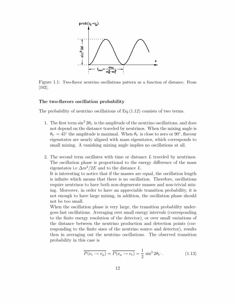
Figure 1.1: Two-flavor neutrino oscillations pattern as a function of distance. From[102].
The two-flavors oscillation probability
The probability of neutrino oscillations of Eq.(1.12) consists of two terms.
1. The first term sin2 2θV is the amplitude of the neutrino oscillations, and doesnot depend on the distance traveled by neutrinos. When the mixing angle isθV = 45 the amplitude is maximal. When θV is close to zero or 90, flavoureigenstates are nearly aligned with mass eigenstates, which corresponds tosmall mixing. A vanishing mixing angle implies no oscillations at all.
2. The second term oscillates with time or distance L traveled by neutrinos.The oscillation phase is proportional to the energy difference of the masseigenstates i.e ∆m2/2E and to the distance L.It is interesting to notice that if the masses are equal, the oscillation lengthis infinite which means that there is no oscillation. Therefore, oscillationsrequire neutrinos to have both non-degenerate masses and non-trivial mix-ing. Moreover, in order to have an appreciable transition probability, it isnot enough to have large mixing, in addition, the oscillation phase shouldnot be too small.When the oscillation phase is very large, the transition probability under-goes fast oscillations. Averaging over small energy intervals (correspondingto the finite energy resolution of the detector), or over small variations ofthe distance between the neutrino production and detection points (cor-responding to the finite sizes of the neutrino source and detector), resultsthen in averaging out the neutrino oscillations. The observed transitionprobability in this case is
P (νe → νµ) = P (νµ → νe) =1
2sin2 2θV . (1.13)
12
1.1.2 3 flavors in vacuum
Consider now the case of three neutrino flavours. Similarly to the two flavourcase, a 3 × 3 unitary mixing matrix relating the flavour eigenstates to the masseigenstates can be defined such as:
νeL
νµL
ντL
=
Ue1 Ue2 Ue3
Uµ1 Uµ2 Uµ3
Uτ1 Uτ2 Uτ3
ν1L
ν2L
ν3L
. (1.14)
In general, in the case of Dirac neutrinos, the lepton mixing matrix U , which ismade of 3 rotation matrices, depends on three mixing angles θ12, θ13 and θ23 andone CP-violating phase δ4. It is convenient to use for the matrix U the standardparametrization of the quark mixing matrix:
U =
c12 c13 s12 c13 s13 e−iδ
−s12 c23 − c12 s23 s13 eiδ c12 c23 − s12 s23 s13 e
iδ s23 c13s12 s23 − c12 c23 s13 e
iδ −c12 s23 − s12 c23 s13 eiδ c23 c13
. (1.15)
One can also factorize the U matrix in three rotation matrices and obtain:
U = T23T13T12D ≡ TD , (1.16)
where
T12 =
c12 s12 0−s12 c12 0
0 0 1
, T13 =
c13 0 s13 e−iδ
0 1 0−s13 e
iδ 0 c13
, T23 =
1 0 00 c23 s23
0 −s23 c23
,
(1.17)and D = diag(e−iϕ1, 1, e−iϕ2). The phases ϕ1 and ϕ2 are present only for neutri-nos in the Majorana case. It immediately follows that the Majorana phases haveno effect on neutrino oscillations. Therefore one can omit the factor D and writeU = T . It can be useful, to factorize T13 as follows
T13 = ST 013S
† (1.18)
4See appendix A.
13
where S(δ) = diag(1, 1, eiδ). For flavor transitions probabilities, following theformula of Eq.(1.19), we have,
P (να → νβ ; t) =
[
3∑
i=1
U∗βi e
iEit Uαi
][
3∑
j=1
Uβj e−iEjt U∗
αj
]
=
3∑
i=1
| Uβi |2 | Uαi |2
+23∑
i<j
Re(Uαi U∗αj U
∗βi Uβj) cos [(Ej −Ei)t]
+23∑
i<j
Im(Uαi U∗αj U
∗βi Uβj) sin [(Ej −Ei)t] . (1.19)
1.1.3 CP-violation in vacuum
It is crucial to underline that in the MNSP matrix (or in the T13 matrix) theCP-violating phase is always multiplied by the sine of the third mixing angle, i.eθ13. Therefore, if θ13 = 0 (which is still currently a possibility) no CP-violationeffects will be observable in the leptonic sector. However, if θ13 6= 0 , then effectsof δ can be seen, at least theoretically. From a more fundamental point of view,the CP symmetry (made of C, the charge conjugation and P, the spatial parity)is the symmetry that converts a left handed neutrino νL into a right handedantineutrino which is the antiparticle of νL. Thus, CP essentially acts as theparticle - antiparticle conjugation. If CP is conserved, the oscillation probabilitybetween particles and their antiparticles coincide:
CP : P (να → νβ; t) = P (να → νβ; t) . (1.20)
However, if the CP symmetry is violated in the leptonic sector, i.e δ 6= 0 , theMNSP matrix is complex (unless θ13 = 0 ). As derived in the appendix C, theaction of the particle – antiparticle conjugation on the lepton mixing matrix Ucan be seen as U → U∗. To search for a CP asymmetry, it is natural to observethe difference of the two probabilities above, namely
∆Pab ≡ P (νa → νb; t)− P (νa → νb; t) . (1.21)
Using the parametrization (1.15) of the mixing matrix U and the equation Eq.(1.19)one finds
∆Peµ = ∆Pµτ = ∆Pτe = 4s12 c12 s13 c213 s23 c23 sin δ
×[
sin
(
∆m212
2Et
)
+ sin
(
∆m223
2Et
)
+ sin
(
∆m231
2Et
)]
.(1.22)
14
1000 2000 3000 4000 5000Distance (km)
-20
-15
-10
-5
0
5
10
15
20
∆P =
P(ν µ
νe)
- (ν
µν e)
[%] δ = 0, π
δ = π/2δ=3π/2
sin22θ13 = 0.05 E = 1 GeV
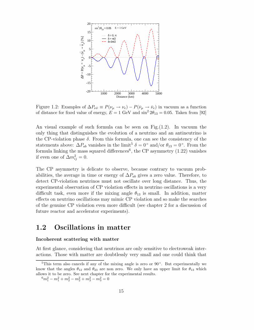
Figure 1.2: Examples of ∆Pνν ≡ P (νµ → νe) − P (νµ → νe) in vacuum as a functionof distance for fixed value of energy, E = 1 GeV and sin2 2θ13 = 0.05. Taken from [92]
An visual example of such formula can be seen on Fig.(1.2). In vacuum theonly thing that distinguishes the evolution of a neutrino and an antineutrino isthe CP-violation phase δ. From this formula, one can see the consistency of thestatements above: ∆Pab vanishes in the limit5 δ = 0 and/or θ13 = 0 . From theformula linking the mass squared differences6, the CP asymmetry (1.22) vanishesif even one of ∆m2
ij = 0.
The CP asymmetry is delicate to observe, because contrary to vacuum prob-abilities, the average in time or energy of ∆Pab gives a zero value. Therefore, todetect CP-violation neutrinos must not oscillate over long distance. Thus, theexperimental observation of CP violation effects in neutrino oscillations is a verydifficult task, even more if the mixing angle θ13 is small. In addition, mattereffects on neutrino oscillations may mimic CP violation and so make the searchesof the genuine CP violation even more difficult (see chapter 2 for a discussion offuture reactor and accelerator experiments).
1.2 Oscillations in matter
Incoherent scattering with matter
At first glance, considering that neutrinos are only sensitive to electroweak inter-actions. Those with matter are doubtlessly very small and one could think that
5This term also cancels if any of the mixing angle is zero or 90 . But experimentally weknow that the angles θ12 and θ23 are non zero. We only have an upper limit for θ13 whichallows it to be zero. See next chapter for the experimental results.
6m21 −m2
1 + m22 −m2
2 + m23 −m2
3 = 0
15
they are negligible. Even in very dense environments, the matter seems almosttransparent for neutrinos which, for instance go through the Sun at the speed oflight when a photon takes about 40000 years to diffuse from the solar core to theouter layer. Actually there are two kinds of scattering, namely the coherent scat-tering and the incoherent one. Let us first focus on the latter. One can estimatethe weak cross section associated to the interactions of neutrino with a chargedlepton or hadron, in the center of mass frame. From dimensional arguments:
σcm ∼ G2F s (1.23)
where s is the Lorentz invariant Mandelstam variable which represents the squareof the total energy. In the laboratory frame, where the target particle is at rest, sis given by 2EM , where E is the neutrino energy and M is the mass of the targetparticle (we neglected the neutrino mass), yielding
σlab ∼ G2FEM ∼ 10−38cm2 EM
GeV2 (1.24)
The mean free path of the neutrino in a medium, with number density N oftarget particles, which are nucleons with mass M ∼ 1 GeV is given by
l ∼ 1
Nσ∼ 1038cm
(N/cm−3)(E/GeV). (1.25)
For example, the Earth has a diameter of ∼ 109cm and the number density Nis ∼ NA cm−3 ∼ 1024 cm−3. Consequently, for neutrinos of energy smaller than∼ 105 GeV, the mean free path will be greater than the Earth’s diameter. Thisis why it is very difficult to detect neutrinos with energy of order ∼ 1MeV.Concerning the Sun, its density varies between ∼ 102NA cm3 at the center to∼ NA cm3 at its surface and for a 1 MeV neutrino, the mean free path will beabout one half of the solar system size! The Sun is therefore transparent for theneutrinos it produces.
Coherent scattering with matter.
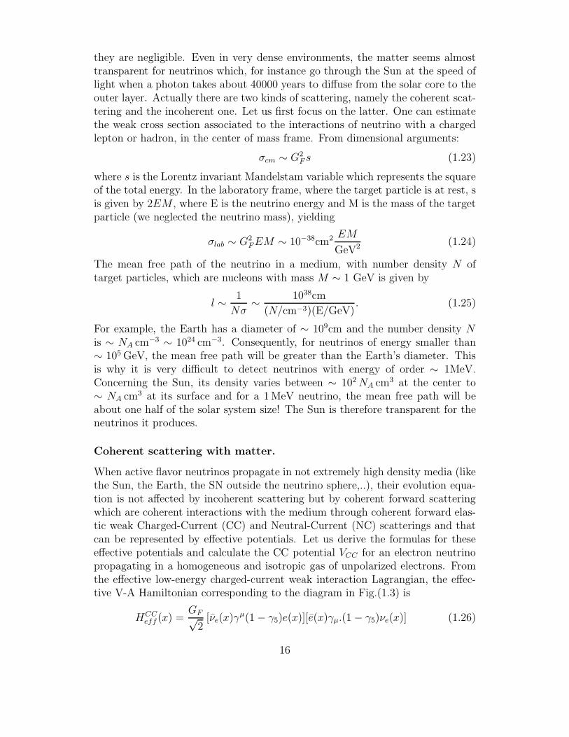
When active flavor neutrinos propagate in not extremely high density media (likethe Sun, the Earth, the SN outside the neutrino sphere,..), their evolution equa-tion is not affected by incoherent scattering but by coherent forward scatteringwhich are coherent interactions with the medium through coherent forward elas-tic weak Charged-Current (CC) and Neutral-Current (NC) scatterings and thatcan be represented by effective potentials. Let us derive the formulas for theseeffective potentials and calculate the CC potential VCC for an electron neutrinopropagating in a homogeneous and isotropic gas of unpolarized electrons. Fromthe effective low-energy charged-current weak interaction Lagrangian, the effec-tive V-A Hamiltonian corresponding to the diagram in Fig.(1.3) is
HCCeff (x) =
GF√2
[νe(x)γµ(1− γ5)e(x)][e(x)γµ.(1− γ5)νe(x)] (1.26)
16
νe e−
νee−
W±
p k′
k p′
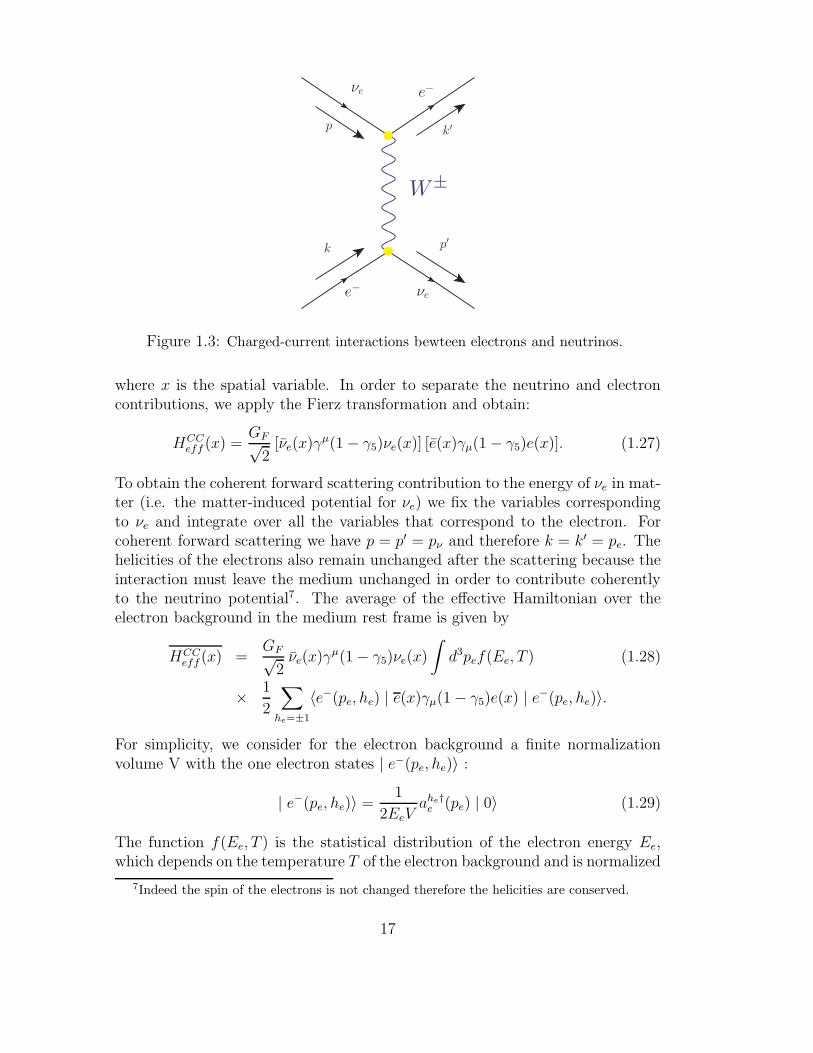
Figure 1.3: Charged-current interactions bewteen electrons and neutrinos.
where x is the spatial variable. In order to separate the neutrino and electroncontributions, we apply the Fierz transformation and obtain:
HCCeff (x) =
GF√2
[νe(x)γµ(1− γ5)νe(x)] [e(x)γµ(1− γ5)e(x)]. (1.27)
To obtain the coherent forward scattering contribution to the energy of νe in mat-ter (i.e. the matter-induced potential for νe) we fix the variables correspondingto νe and integrate over all the variables that correspond to the electron. Forcoherent forward scattering we have p = p′ = pν and therefore k = k′ = pe. Thehelicities of the electrons also remain unchanged after the scattering because theinteraction must leave the medium unchanged in order to contribute coherentlyto the neutrino potential7. The average of the effective Hamiltonian over theelectron background in the medium rest frame is given by
HCCeff (x) =
GF√2νe(x)γ
µ(1− γ5)νe(x)
∫
d3pef(Ee, T ) (1.28)
× 1
2
∑
he=±1
〈e−(pe, he) | e(x)γµ(1− γ5)e(x) | e−(pe, he)〉.
For simplicity, we consider for the electron background a finite normalizationvolume V with the one electron states | e−(pe, he)〉 :
| e−(pe, he)〉 =1
2EeVahe†
e (pe) | 0〉 (1.29)
The function f(Ee, T ) is the statistical distribution of the electron energy Ee,which depends on the temperature T of the electron background and is normalized
7Indeed the spin of the electrons is not changed therefore the helicities are conserved.
17
by:∫
d3pef(Ee, T ) = NeV (1.30)
where Ne is the electron density of the medium and NeV is the total number ofelectrons. The average over helicities of the electron matrix element is given by:
1
2
∑
he=±1
〈e−(pe, he) | e(x)γµ(1− γ5)e(x) | e−(pe, he)〉
=1
4EeV
∑
he=±1
u(he)e (pe)γµ(1− γ5)u
(he)e (pe)
=1
4EeVTr[
(/pe+me)γµ(1− γ5)
]
=1
4EeVTr [(pα
e γαγµ − pαe γαγµγ5 +meγµ −meγµγ5] =
(pe)µ
EeV(1.31)
where the last three terms give zero. Hence, we obtain
HCCeff (x) =
GF√2
1
V
∫
d3pef(Ee, T )νe(x)/pe
Eeνe(x) (1.32)
The integral over d3pe gives:
∫
d3pef(Ee, T )/pe
Ee
(1− γ5)
=
∫
d3pef(Ee, T )
(
γ0 −−→pe .−→γ
Ee
)
= NeV γ0. (1.33)
Indeed, the second term vanishes because the integrand is odd under −→pe → −−→pe .Finally, the normalization volume cancels, and we use the left projector8 PL =(1− γ5)/2 to obtain left-handed neutrinos which leads to
HCCeff (x) = VCC νeL(x)γ0νeL(x) (1.34)
where the CC potential is given by:
VCC = Ve =√
2GFNe . (1.35)
Analogously, one can find the NC contributions VNC to the matter-inducedneutrino potentials. Since NC interaction are flavour independent, these con-tributions are the same for neutrinos of all three flavours. The neutral-currentpotential of neutrinos propagating in a medium with density Nf of fermions f
8In addition, we use the property of the projector namely 2PL = 2P 2L
18
νe νe
e−e−
Z0
p p′
k k′
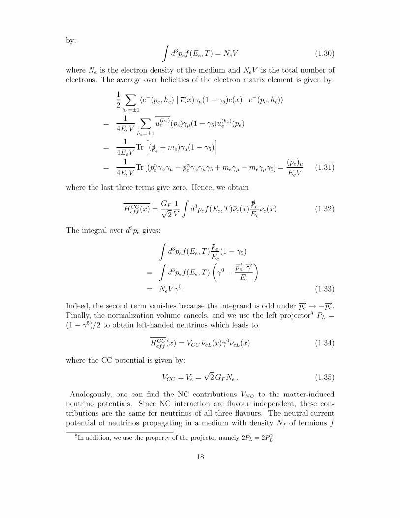
Figure 1.4: Neutral-current interactions between fermions and all type of neutrinos.
can be calculated in a similar way. Starting from the effective low-energy neutral-current weak interaction Hamiltonian corresponding to the diagram in Fig.(1.4)we have:
HCCeff (x) =
GF√2
∑
α=e,µ,τ
[να(x)γµ(1− γ5)να(x)]∑
f
[f(x)γµ(1− γ5)f(x)]. (1.36)
Comparing with the effective CC Hamiltonian which generates the potentialin Eq.(1.35) one can see that the neutral-current potential of any flavor neutrinoνα due to coherent interaction with fermions f is:
V fNC =
∑
f
√2GFNf g
fV . (1.37)
For electrons we have:
geV = −1
2+ 2 sin2 θW (1.38)
Since p = uud and n = udd, we have for protons:
gpV = 2gu
V + gdV =
1
2− 2 sin2 θW , (1.39)
and for neutrons:
gnV = gu
V + 2gdV = −1
2. (1.40)
For the astrophysical environments we are interested in, such as the Sun or asupernova, locally matter is composed of neutrons, protons, and electrons. Sinceelectrical neutrality implies an equal number density of protons and electrons,
19
the neutral-current potentials of protons and electrons cancel each other andonly neutrons contribute, yielding
VNC = −1
2
√2GFNn (1.41)
Together with Eq.(1.35) we can write the effective matter Hamiltonian:
Hm =
Ve + Vn 0 00 Vn 00 0 Vn
. (1.42)
Since one cannot observe wave functions of neutrinos but only the oscillationprobabilities, every term proportional to the identity matrix gives a commonphase that we can get rid of. The effective Hamiltonian is finally:
Hm =
Ve 0 00 0 00 0 0
. (1.43)
Note that for antineutrinos, one has to replace Va → −Va. It is Wolfensteinthat discovered in 1978, that neutrinos propagating in matter are subject to apotential due to the coherent forward elastic scattering with the particles in themedium (electrons and nucleons)[117]. This potential, which is equivalent to anrefraction index, modifies the mixing of neutrinos.
1.2.1 The Mikheyev-Smirnov-Wolfenstein (MSW) effect
Following the work of Wolfenstein, Mikheyev and Smirnov in 1986 show thepossibility of a resonant conversion in a non-constant matter density profile [89,90]. It is natural to write the neutrino evolution equation in matter in the flavourbasis since they interact with matter via the electroweak bosons.
id
dt
(
νe
νµ
)
=
(
−∆m2
4Ecos 2θV +
√2
2GFNe
∆m2
4Esin 2θV
∆m2
4Esin 2θV
∆m2
4Ecos 2θV −
√2
2GFNe
)
(
νe
νµ
)
,
(1.44)where θV is the vacuum mixing angle. From this equation we can think of newneutrino states, the matter states, related to the flavour states by:
(
νm1
νm2
)
= U †m(t)
(
νe
νµ
)
=
(
cos θm(t) − sin θm(t)sin θm(t) cos θm(t)
)(
νe
νµ
)
, (1.45)
where Um(t) is the matter mixing matrix with θm(t) the associated matter mixingangle associated. These two quantities depend on time (or distance) because ofthe matter density profile which varies with time (or distance). Actually, these
20
matter states are the instantaneous matter eigenstates which allow a instanta-neous diagonalization of the effective Hamiltonian written in the flavour basisHfv as in Eq.(1.44):
Um(t)†Hfv(t)Um(t) = Hd(t) = diag(Em1(t), Em2(t)) . (1.46)
with Em1(t) and Em2(t) are instantaneous eigenvalues of Hfv(t). The evolutionequation in the basis of the instantaneous eigenstates can therefore be written asi(d/dt)ν = [Hd − iU †
m(dUm/dt)]ν, or
id
dt
(
νm1
νm2
)
=
(
Em1(t) −iθm(t)
iθm(t) Em2(t)
)(
νm1
νm2
)
, (1.47)
where θm ≡ dθm/dt. Notice that the effective matter Hamiltonian in this basis isnot diagonal since the mixing angle θm(t) is not constant, i.e. the matter eigen-state basis changes with time. To obtain the oscillation probability equationswith the same simple form as in vacuum, we can study the case where the matterdensity (and chemical composition) is taken constant (i.e Ne = const). There-fore, we obtain a diagonal effective Hamiltonian for the matter eigenstates sincedUm/dt = 0 just like the vacuum Hamiltonian is diagonal in the mass basis. Toderive an explicit oscillation probability equation one has to express the mattermixing angle as a function of density and the vacuum mixing angle, by linkingthe matter basis to the flavour basis. Starting from Eq.(1.47) with no off-diagonalterms, and rotating in the favour basis, one obtains, after removing the diagonal(Em1(t) + Em2(t))/2:
id
dt
(
νe
νµ
)
=(Em1(t)−Em2(t))
2
(
cos 2θm(t) sin 2θm(t)sin 2θm(t) − cos 2θm(t)
)(
νe
νµ
)
. (1.48)
By comparing this form of the effective Hamiltonian in the flavour basis to thefirst one given in Eq.(1.44), one obtains the two following relations:
sin 2θm =∆m2
2Esin 2θV
Em1(t)−Em2(t)(1.49)
cos 2θm =−∆m2
2Ecos 2θV +
√2GF Ne
Em1(t)− Em2(t). (1.50)
Em1(t) and Em2(t) are easily found by diagonalizing the effective Hamiltonian ofEq.(1.44) and their difference is :
Em1(t)− Em2(t) =
√
(
∆m2
2Ecos 2θV −
√2GF Ne
)2
+
(
∆m2
2E
)2
sin2 2θV (1.51)
21
As said before if the Hamiltonian in the matter basis is diagonal then the oscilla-tion probability will have exactly the same form as in vacuum. For instance theprobability of νe ↔ νµ oscillations in matter is :
P (νe → νµ; L) = sin2 2θm sin2
(
πL
lm
)
, (1.52)
where
lm =2π
Em1 − Em2
=2π
√
(
∆m2
2Ecos 2θV −
√2GF Ne
)2+(
∆m2
2E
)2sin2 2θV
. (1.53)
Comparing with the vacuum formula of Eq.(1.7), the vacuum mixing angle θV
and oscillation length losc are replaced by those in matter, θm and lm. In the limitof zero matter density, we have θ = θV , lm = losc, and the vacuum oscillationprobability is recovered. Let us look more closely at the oscillation amplitude ofEq.(1.52)
sin2 2θm =
(
∆m2
2E
)2
sin2 2θV
(
∆m2
2Ecos 2θV −
√2GF Ne
)2+(
∆m2
2E
)2sin2 2θV
. (1.54)
It has a typical resonance form, with the maximum value sin2 2θm = 1 achievedwhen the condition √
2GF Ne =∆m2
2Ecos 2θV (1.55)
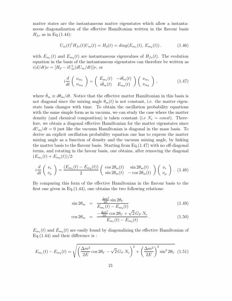
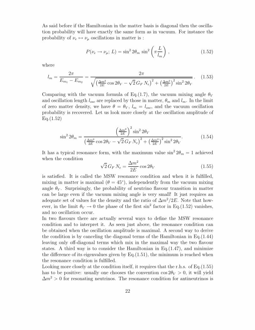
is satisfied. It is called the MSW resonance condition and when it is fulfilled,mixing in matter is maximal (θ = 45), independently from the vacuum mixingangle θV . Surprisingly, the probability of neutrino flavour transition in mattercan be large even if the vacuum mixing angle is very small! It just requires anadequate set of values for the density and the ratio of ∆m2/2E. Note that how-ever, in the limit θV → 0 the phase of the first sin2 factor in Eq.(1.52) vanishes,and no oscillation occur.In two flavours there are actually several ways to define the MSW resonancecondition and to interpret it. As seen just above, the resonance condition canbe obtained when the oscillation amplitude is maximal. A second way to derivethe condition is by canceling the diagonal terms of the Hamiltonian in Eq.(1.44)leaving only off-diagonal terms which mix in the maximal way the two flavourstates. A third way is to consider the Hamiltonian in Eq.(1.47), and minimizethe difference of its eigenvalues given by Eq.(1.51), the minimum is reached whenthe resonance condition is fulfilled.Looking more closely at the condition itself, it requires that the r.h.s. of Eq.(1.55)has to be positive: usually one chooses the convention cos 2θV > 0, it will yield∆m2 > 0 for resonating neutrinos. The resonance condition for antineutrinos is
22
then ∆m2 < 0 since one gets an opposite matter potential sign in the effectiveHamiltonian.9 Therefore, for a given sign of ∆m2, either neutrinos or antineutri-nos (but not both) can experience the resonantly enhanced oscillations in matter.This is how we deduced that ∆2m21 > 0: electron neutrinos undergo a MSW res-onance in the Sun as we will discuss more in the next chapter.Finally, in a more realistic case where matter density varies, like the Sun whereneutrinos are produced with a certain spectrum in energy, one can realize that theresonance condition does not involve any fine tuning: if ∆m2 is of the right orderof magnitude, then for any value of the matter density there is a value of neutrinoenergy for which the resonance condition (1.55) is satisfied and vice-versa. Thisis tru only if the condition of adiabaticity is fulfilled (See appendix B).
1.2.2 3 flavours in matter
In Nature, neutrinos exist in 3 flavours mixed by the MNSP matrix and can inter-act coherently with matter giving rise to a matter potential in the Hamiltonian.When one takes into account 3 flavours neutrinos in matter, at the tree level,two resonances might occur, one called the high resonance (H-resonance) whichrequires a high density and a low resonance (L-resonance) which happen at lowerdensity10. Such phenomena can occur if the matter density if sufficiently high,like in the supernova environment. Approximations can be made to handle theproblem analytically, but a numerical calculation is required if one wants to keepall the physical information encoded in the neutrino fluxes while propagatingthrough matter.
MSW resonances in 3 flavours
Contrary to the 2 flavour case, it is difficult to define an MSW resonance con-dition in 2 flavours. In fact, different ways used previously, like for instance themaximization of the amplitude of the oscillation probability, or minimization ofthe difference between the eigenvalues of the effective Hamiltonian in matter, leadto different results. Following the derivation of the MSW in section 1.2.1, we can
9One can also considers that ∆m2 is always postive. If the angle is between 0 and 45 itcorresponds to the normal hierarchy, if the range is 45 to 90 then it is inverted hierachy.
10Actually, when one considers one loop corrections for neutrino interacting with matter,a supplementary potential appears, named Vµτ which can be seen as an effective presenceof τ in the medium. Its inclusion introduces an extra resonance, deep inside the supernova.Nevertheless, such resonance depends on the hierarchy, the mixing angles, and if θ23 is largeror smaller than 45. A detailed study has been recently performed in [80]. The hypothesisusually made is that Vµτ engenders no change of the fluxes at the resonance but just a mixingbetween the concerned states. This assumption is valid only if one considers that the νµ flux isequal to the ντ flux.
23
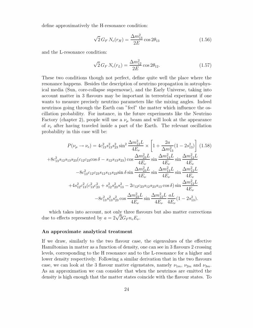
define approximatively the H-resonance condition:
√2GF Ne(rH) =
∆m213
2Ecos 2θ13 (1.56)
and the L-resonance condition:
√2GF Ne(rL) =
∆m212
2Ecos 2θ12. (1.57)
These two conditions though not perfect, define quite well the place where theresonance happens. Besides the description of neutrino propagation in astrophys-ical media (Sun, core-collapse supernovae), and the Early Universe, taking intoaccount matter in 3 flavours may be important in terrestrial experiment if onewants to measure precisely neutrino parameters like the mixing angles. Indeedneutrinos going through the Earth can ”feel” the matter which influence the os-cillation probability. For instance, in the future experiments like the NeutrinoFactory (chapter 2), people will use a νµ beam and will look at the appearanceof νe after having traveled inside a part of the Earth. The relevant oscillationprobability in this case will be:
P (νµ → νe) = 4c213s213s
223 sin2 ∆m2
13L
4Eν×[
1 +2a
∆m213
(1− 2s213)
]
(1.58)
+8c213s12s13s23(c12c23cos δ − s12s13s23) cos∆m2
23L
4Eνsin
∆m213L
4Eνsin
∆m212L
4Eν
−8c213c12c23s12s13s23sin δ sin∆m2
23L
4Eνsin
∆m213L
4Eνsin
∆m212L
4Eν
+4s212c
213(c
213c
223 + s2
12s223s
213 − 2c12c23s12s23s13 cos δ) sin
∆m212L
4Eν
−8c213s213s
223 cos
∆m223L
4Eν
sin∆m2
13L
4Eν
aL
4Eν
(1− 2s213).
which takes into account, not only three flavours but also matter correctionsdue to effects represented by a = 2
√2GFneEν .
An approximate analytical treatment
If we draw, similarly to the two flavour case, the eigenvalues of the effectiveHamiltonian in matter as a function of density, one can see in 3 flavours 2 crossinglevels, corresponding to the H resonance and to the L-resonance for a higher andlower density respectively. Following a similar derivation that in the two flavourscase, we can look at the 3 flavour matter eigenstates, namely ν1m, ν2m and ν3m.As an approximation we can consider that when the neutrinos are emitted thedensity is high enough that the matter states coincide with the flavour states. To
24
know to which matter eigenstates corresponds which flavour eigenstates, we usethe evolution operator in matter:
νm1L
νm2L
νm3L
=
Um1e Um
1µ Um1τ
Um2e Um
2µ Um3µ
Um3e Um
2τ Um3τ
νeL
νµL
ντL
. (1.59)
Since the evolution operator of Eq.(1.59) linking the matter eigenstates to theflavour eigenstates must correspond at zero density to the MNSP matrix, we candefine three matter mixing angles11: θm
13, θm23, and θm
12. In the previous section wehave seen that in the approximation of infinite density, the matter mixing angletends to the value π/2. This yields:
ν1m = νµ , ν2m = ντ , ν3m = νe . (1.60)
Probabilities of conversion in dense matter
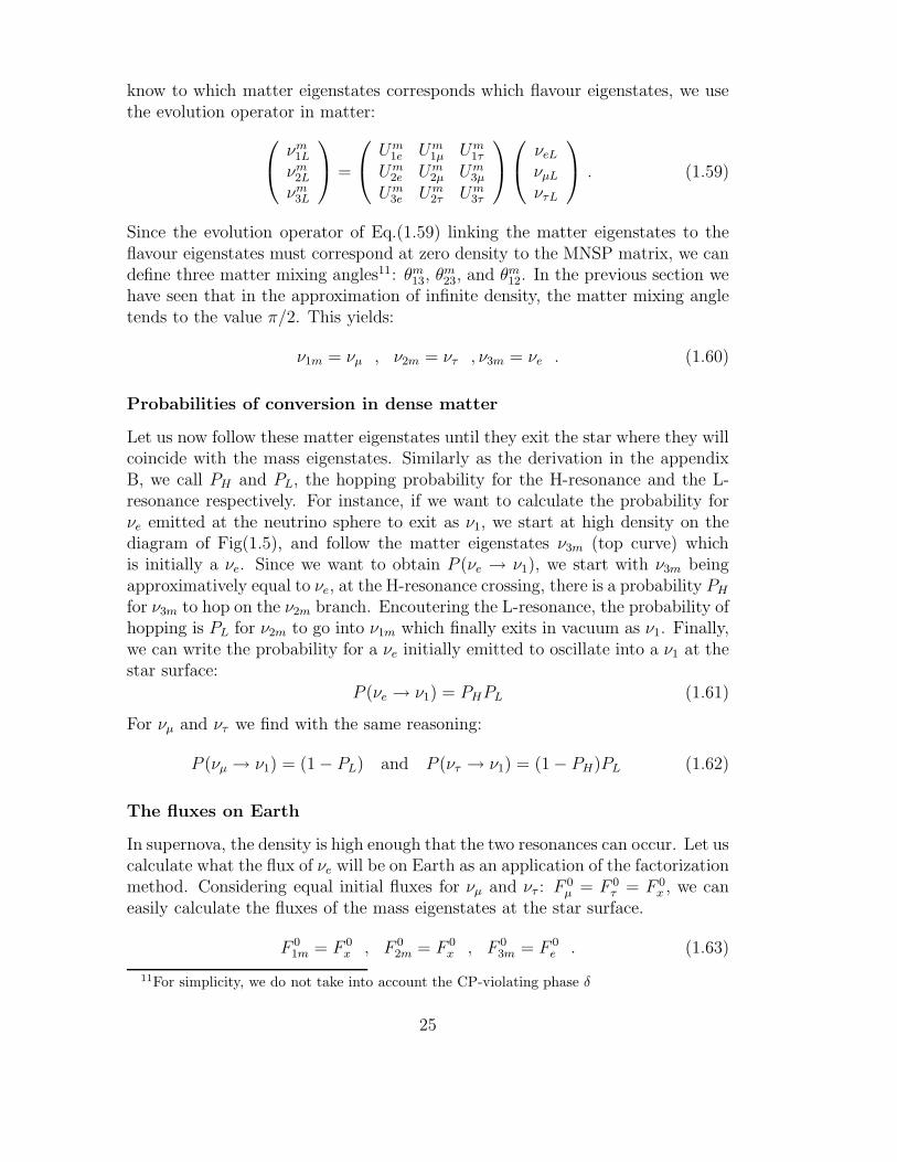
Let us now follow these matter eigenstates until they exit the star where they willcoincide with the mass eigenstates. Similarly as the derivation in the appendixB, we call PH and PL, the hopping probability for the H-resonance and the L-resonance respectively. For instance, if we want to calculate the probability forνe emitted at the neutrino sphere to exit as ν1, we start at high density on thediagram of Fig(1.5), and follow the matter eigenstates ν3m (top curve) whichis initially a νe. Since we want to obtain P (νe → ν1), we start with ν3m beingapproximatively equal to νe, at the H-resonance crossing, there is a probability PH
for ν3m to hop on the ν2m branch. Encoutering the L-resonance, the probability ofhopping is PL for ν2m to go into ν1m which finally exits in vacuum as ν1. Finally,we can write the probability for a νe initially emitted to oscillate into a ν1 at thestar surface:
P (νe → ν1) = PHPL (1.61)
For νµ and ντ we find with the same reasoning:
P (νµ → ν1) = (1− PL) and P (ντ → ν1) = (1− PH)PL (1.62)
The fluxes on Earth
In supernova, the density is high enough that the two resonances can occur. Let uscalculate what the flux of νe will be on Earth as an application of the factorizationmethod. Considering equal initial fluxes for νµ and ντ : F
0µ = F 0
τ = F 0x , we can
easily calculate the fluxes of the mass eigenstates at the star surface.
F 01m = F 0
x , F 02m = F 0
x , F 03m = F 0
e . (1.63)
11For simplicity, we do not take into account the CP-violating phase δ
25
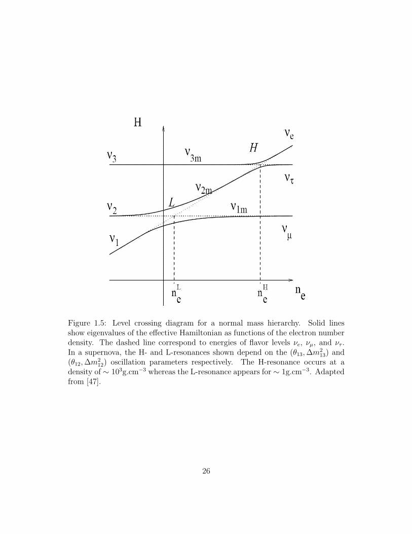
Figure 1.5: Level crossing diagram for a normal mass hierarchy. Solid linesshow eigenvalues of the effective Hamiltonian as functions of the electron numberdensity. The dashed line correspond to energies of flavor levels νe, νµ, and ντ .In a supernova, the H- and L-resonances shown depend on the (θ13,∆m
213) and
(θ12,∆m212) oscillation parameters respectively. The H-resonance occurs at a
density of ∼ 103g.cm−3 whereas the L-resonance appears for ∼ 1g.cm−3. Adaptedfrom [47].
26
Consequently, using Eqs. (1.61) and (1.62), the total ν1 flux at the surface of thestar equals the sum of the three contributions:
F1 = PHPLF0e + (1− PHPL)F 0
x . (1.64)
Similarly, the fluxes of neutrino mass eigenstates ν2 and ν3 arriving at the surfaceof the star are
F2 = PH(1− PL)F 0e + (1 + PH(PL − 1)F 0
x ,
F3 = (1− PH)F 0e + PHF
0x . (1.65)
The interest of looking at the fluxes of mass eigenstates is because these areeigenstates of the vacuum Hamiltonian. Each state evolves independently invacuum and acquires a phase. Therefore, from the stars to Earth, a spreadwill occur for the wave packets, any coherence between the mass eigenstateswill be lost on the way to Earth. The neutrinos arriving at the surface of theEarth as incoherent fluxes of the mass eigenstates, we have to perform anothertransformation to obtain flavour fluxes to which experiments are sensitive. Tocalculate the νe flux on Earth12, one has to multiply the flux associated to eachmass eigenstate by the probability to get a νe from a mass eigenstate i:
Fe = F1P (ν1 → νe) + F2P (ν2 → νe) + F3P (ν3 → νe) (1.66)
where the decoherence among the mass eigenstates is explicit. The P (νi → νe)probabilities are nothing but the squared modulus of the corresponding elementsof the MNSP matrix (given by Eq.()):
Fe = |Ue1|2F1 + |Ue2|2F2 + |Ue3|2F3 (1.67)
Taking into account the unitarity condition∑
|Uei|2 = 1, we can write the finalelectron neutrino flux reaching the Earth:
Fe = pF 0e + (1− p)F 0
x , (1.68)
wherep = |Ue1|2PHPL + |Ue2|2(1− PL)PH + |Ue3|2(1− PH) . (1.69)
According to (1.68), p may be interpreted as the total survival probability of elec-tron neutrinos. Note that the final fluxes of the flavor states at the Earth like inEq.(1.68) can be written only in terms of the survival probability p. In conclusion,what occurs in a medium like supernovae, depends on the hopping probability ofthe H- and the L-resonances and the associated adiabaticity (PH,L = 0) or non-adiabaticity (PH,L = 1) of the transition. In the Landau-Zener approximation,the hopping probability has an explicit dependence upon θ, ∆m2 and dNe/dr. In
12Up to an implicit geometrical factor of 1/(4πL2) in the fluxes on Earth
27
0 5 10 15 20distance in units of 100 km
0
0.2
0.4
0.6
0.8
1
Pro
babi
lity
Figure 1.6: Numerical calculation of the electron neutrino survival probability ina supernova with 1/r3 density profile. The black curve shows a 3 flavour adiabaticH-resonance with θ13 = 9. When θ13 = 0.5, the H-resonance (around 400 km)is much less adiabatic and induces only a small conversion (red curve). In thiscase, the L-resonance (around 1200 km) is possible since the first encounteredwas only slightly adiabatic. When one considers only a 2 flavour system, we cansee that the H-resonance is almost the same as in 3 flavours because the greendashed curve (θ13 = 9) is almost superimposed to the black curve which meansthe 2 flavour approximation is good for the H-resonance. In the case of a smallθ13, the blue curve (2 flavours) is superimposed to the red curve but does notencounter a second resonance because it is a 2 flavour calculation. Note here thatthe hierarchy is normal.
a supernova, the L-resonance is determined by the solar parameters ∆m212 and
θ12 which are well established and renders the transition adiabatic (See appendixB) for general density profiles from SN simulations. Since ∆m2
12 is positive, theresonance always occur in the νe channel. On the other hand, the H-resonancedepends on the θ13 value and the sign of ∆m2
13 which are still unknown. Suchinformation is embedded in a supernova signal. This is why one might use fu-ture observations from (extra-) galactic Supernova explosion or relic supernovaneutrinos to learn about neutrino properties.
28
The approximations in the analytical treatment
To obtain such result we made several approximations. First, we made the ap-proximation that, at each transition, one of the neutrinos is decoupled so that thecalculation of probability reduces to a 2 flavours problem, which can be a goodapproximation (see Fig.(1.6)). Such an approximation could be avoided if theevolution of the three matter eigenstates were perfectly adiabatic. This wouldmean that the effective matter Hamiltonian could be diagonal all along the evo-lution of neutrinos from the neutrino sphere to the surface of the star. This isof course not the case, since we can only make an instantaneous diagonalizationof the Hamiltonian. Therefore, each neutrinos interfere with the two others atevery moment.Second, the factorization can be performed because we suppose that the two res-onances are well separated and do not influence each other. This approximationis reasonable because, for instance in supernova, at least an order of magnitudeseparate in distance the two resonances, due to the fact that there are two scalesof ∆m2, namely ∆m2
13/∆m212 ∼ 40.
The third approximation made was to consider that the matter eigenstates areequal to the flavour eigenstates initially, which is true only in the approximationof an initial infinite density. Fourth and last approximation, we consider thatthe fluxes of νµ and ντ were equal at the neutrino sphere. This approximation isquite good depending on the studied problem, and was made here for a questionof simplicity.
The analytical treatment just described, with the factorization approxima-tions, has been extensively used in the literature since it gives quite accuratephysical results. However the first approximation has actually an importantdrawback, it only considers factorized transition probabilities and neglects allpossible phase effects between the eigenstates. It also neglects the CP-violatingphase. As we are going to see from our results (chapter 4, 6 and 7), such ap-proximation can therefore miss relevant physics. Only a complete numerical codewhich solves with a good accuracy the system of coupled differential equationsdescribing exactly the neutrino evolution in media can encode all the interestingand relevant physical phenomena, as we will discuss in the following.
29

30
Chapter 2
Neutrino oscillations: theexperimental results andperspectives
Since the first neutrino experiment in 1956 by Cowan and Reines [36], incredibleprogress has been made in the search for neutrino properties. One of the most im-portant one is the discovery of the oscillation phenomenon by Super-Kamiokandein 1998. Many neutrino experiments are currently running and several futureexperiments have been financially approved. Their goal is the same, improve ourknowledge of the MNSP matrix and in particular experiments are rather turnedto the improvement of the third mixing angle, the CP-violation phase (which arethe two unknown parameters of the mixing matrix) and search to discriminatethe hierarchy of neutrinos1.
2.1 The solar data: θ12 and ∆m221
2.1.1 The Standard Solar Model (SSM)
In the 20’s, Eddington advocated the theory that proton-proton reactions werethe basic principle by which the Sun and other stars burn. In the 30’s, anotherprocess for the stars to burn was proposed by Weizsacker and Bethe [28] indepen-dently in 1938 and 1939, it is called the CNO cycle. Those two processes implyan important production of electron neutrinos. Later on, it became clear thatstars are powerful neutrino sources.By the 1960’s our understanding of the solar interior, and of low energy nuclearphysics, had reached such a stage that the Sun’s output could be predicted with
1One of the main concerns is the question of their nature, i.e whether they are Dirac orMajorana types. See appendix A for a brief discussion. Other open issues concern for instancethe neutrino magnetic moment, or the existence of sterile neutrinos.
31
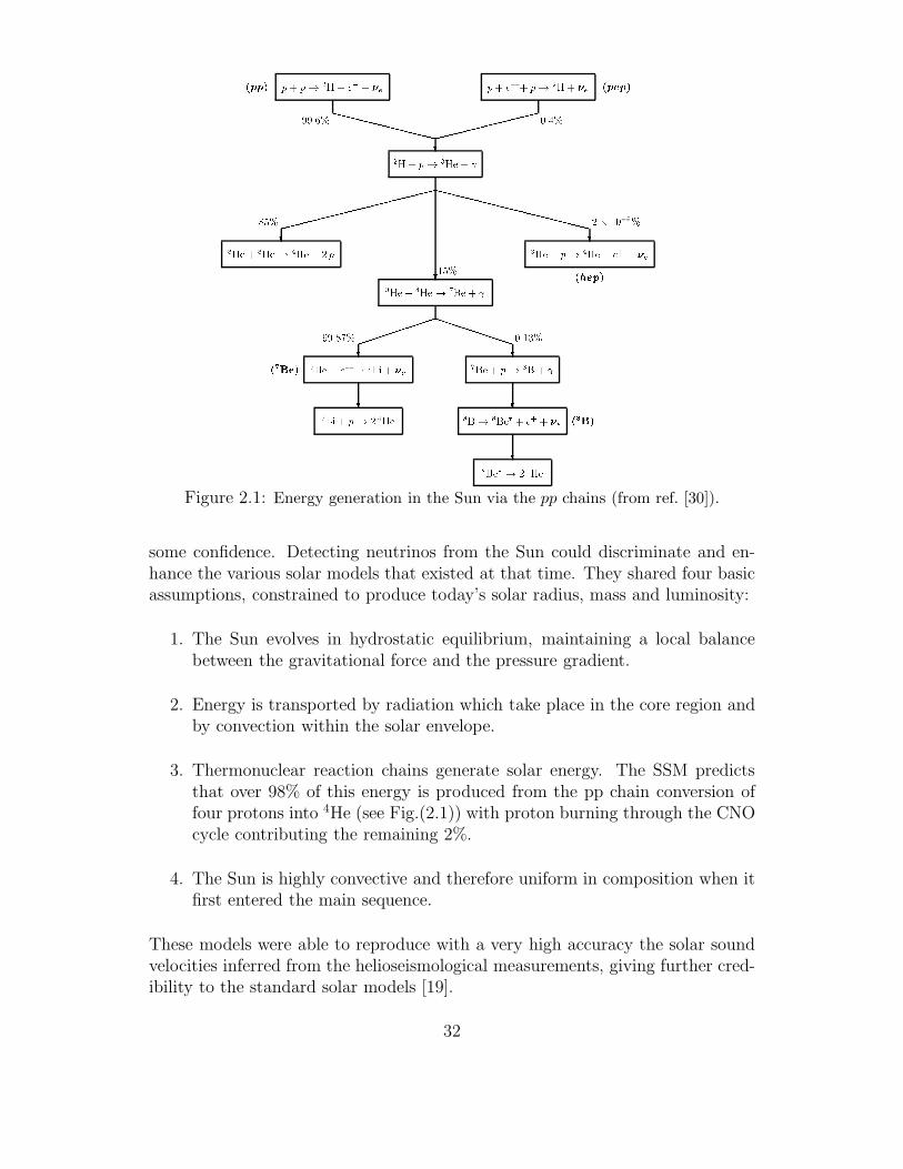
(pp) p+ p! 2H+ e+ + e99.6% XXXXXXXXXXXX (pep)p+ e + p! 2H+ e0.4%?2H+ p! 3He+ 85%?3He+ 3He! 4He + 2 p XXXXXXXXXXXXXXXXXX 2 105%?3He+ p! 4He+ e+ + e(hep)?15%3He+ 4He! 7Be + 99.87% ?7Be + e ! 7Li + e(7Be) ?7Li + p! 2 4He PPPPPPPPP 0.13%?7Be + p! 8B + ?8B! 8Be + e+ + e (8B)?8Be ! 2 4HeFigure 2.1: Energy generation in the Sun via the pp chains (from ref. [30]).
some confidence. Detecting neutrinos from the Sun could discriminate and en-hance the various solar models that existed at that time. They shared four basicassumptions, constrained to produce today’s solar radius, mass and luminosity:
1. The Sun evolves in hydrostatic equilibrium, maintaining a local balancebetween the gravitational force and the pressure gradient.
2. Energy is transported by radiation which take place in the core region andby convection within the solar envelope.
3. Thermonuclear reaction chains generate solar energy. The SSM predictsthat over 98% of this energy is produced from the pp chain conversion offour protons into 4He (see Fig.(2.1)) with proton burning through the CNOcycle contributing the remaining 2%.
4. The Sun is highly convective and therefore uniform in composition when itfirst entered the main sequence.
These models were able to reproduce with a very high accuracy the solar soundvelocities inferred from the helioseismological measurements, giving further cred-ibility to the standard solar models [19].
32
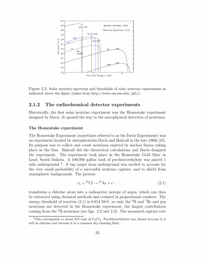
Figure 2.2: Solar neutrino spectrum and thresholds of solar neutrino experiments asindicated above the figure (taken from http://www.sns.ias.edu/ jnb/).
2.1.2 The radiochemical detector experiments
Historically, the first solar neutrino experiment was the Homestake experimentdesigned by Davis. It opened the way to the astrophysical detection of neutrinos.
The Homestake experiment
The Homestake Experiment (sometimes referred to as the Davis Experiment) wasan experiment headed by astrophysicists Davis and Bahcall in the late 1960s [45].Its purpose was to collect and count neutrinos emitted by nuclear fusion takingplace in the Sun. Bahcall did the theoretical calculations and Davis designedthe experiment. The experiment took place in the Homestake Gold Mine inLead, South Dakota. A 100,000 gallon tank of perchloroethylene was placed 1mile underground 2. A big target deep underground was needed to account forthe very small probability of a successful neutrino capture, and to shield fromatmospheric backgrounds. The process
νe + 37Cl→ 37Ar + e− . (2.1)
transforms a chlorine atom into a radioactive isotope of argon, which can thenbe extracted using chemical methods and counted in proportional counters. Theenergy threshold of reaction (2.1) is 0.814 MeV, so only the 8B and 7Be and pepneutrinos are detected in the Homestake experiment, the largest contributioncoming from the 8B neutrinos (see figs. 2.2 and 2.3). The measured capture rate
2This corresponds to about 615 tons of C2Cl4. Perchloroethylene was chosen because it isrich in chlorine and because it is a common dry-cleaning fluid.
33
2.56 ± 0.23 SNU (1 SNU = 10−36 capture /atom /sec) is about one third whatgives the SSM. This experiment was the first one to realize the solar neutrinoproblem.
SAGE and GALLEX experiments
Radiochemical techniques are also used in two other solar neutrino experiments:SAGE was based at the Baksan Neutrino Observatory in the Caucasus moun-tains in Russia and ran between 1990 and 1993. GALLEX was located in theunderground astrophysical laboratory Laboratori Nazionali del Gran Sasso in theItalian Abruzzo province and ran between 1991 and 1997. A followed-up to theGALLEX experiment was the Gallium solar Neutrino Observatory (GNO) whichheld series of measurements between May 1998 - Jan 2002 [38]. The reactioninvolved in these experiments is:
νe + 71Ga→ 71Ge + e− . (2.2)
The energy threshold of this reaction is 0.234 MeV, and so the gallium experi-ments can also detect the lowest energy pp neutrinos. Since the flux of the ppneutrinos is very large, they are expected to give the main contribution to theevent rates in the SAGE and Gallex detectors (Fig. 2.3). The experimental cap-ture rates are respectively 67 ± 5 SNU for the SAGE experiment [3] and 69 ± 5SNU for the GALLEX experiment where the SSM predictions is about 130 SNU[11, 71].
2.1.3 The Cherenkov detector experiments.
This type of experiment exploits water Cerenkov detectors to view solar neu-trinos on an event-by-events basis in contrast to the radiochemical detectorssuch as Homestake, GALLEX, and SAGE, which can only determine a time- andenergy-integral of the flux. Solar neutrinos scatter off electrons, with the recoilingelectrons producing the Cerenkov radiation that is then recorded in surroundingphototubes.
Kamiokande and Super-Kamiokande(Super-K)
Kamiokande and its up-scaled version Super-Kamiokande are water Cherenkovdetectors whose primary purpose was to detect whether proton decay exists,one of the most fundamental questions of elementary particle physics. Thosedetectors are based in the city of Hida, Japan. The detector, named Kamiokandefor Kamioka Nucleon Decay Experiment, constructed in 1983 containing 3,000tons of pure water and about 1,000 photomultiplier tubes (PMTs) attached to itsinner surface. The detector was upgraded, starting in 1985, to allow it to observesolar neutrinos. Its upgraded version is called Super-Kamiokande, and consists
34
of a cylindrical stainless steel tank holding 50,000 tons of ultra-pure water. It isoverseen by about 11100 photomultipliers tubes able to detect Cherenkov light.The neutrino-electron scattering reaction concerned to detect solar neutrinos is
νa + e− → νa + e− . (2.3)
This reaction has zero physical threshold, but one has to introduce energy cutsto suppress the background. In the Kamiokande experiment solar neutrinos withthe energies E > 7.5 MeV were detected, whereas the threshold used by Super-Kamiokande was 5.5 MeV. With these energy cuts, the Kamiokande and Super-Kamiokande detection rates are only sensitive to the 8B component of the solarneutrino flux3. Compared to the radiochemical experiments, Cerenkov detectorsare able to detect the direction of the sources. Indeed, the electrons coming fromthis reaction are confined to a forward cone. Hence detecting the Cerenkov radia-tion from the final electron one can determine neutrino’s direction4. Moreover, forneutrino energies E ≫ me, the angular distribution of the reaction (2.3) pointsin the direction of the momentum of the incoming neutrino. The angular distri-butions of neutrinos detected in the Kamiokande and Super-Kamiokande exper-iments have a prominent peak at 180 from the direction to the sun. The abilityof the Kamiokande experiment to observe the direction of electrons produced insolar neutrino interactions allowed experimentalists to directly demonstrate forthe first time that the Sun was the source of the neutrinos detected.
2.1.4 The solar neutrino problem
In all five solar neutrino experiments, fewer neutrinos than expected were de-tected, the degree of deficiency being different in the experiments of differenttypes (fig. 2.3). The solar neutrino problem is not just the problem of thedeficit of the observed neutrino flux: results of different experiments seem to beinconsistent with each other. Many explanations for this neutrino deficit wereproposed:
1. The most obvious explanation could be the presence of experimental errors,such as miscalculated detection efficiency or cross section. The fact is thatall the solar neutrino experiments but one (Homestake5) have been cali-brated, and their experimental responses were found to be in a very goodagreement with expectations.
3The detection rates are also sensitive to hep fluxes but their contribution is small comparedto the 8B component of the solar neutrino flux.
4Nevertheless, in this type of reaction it is very difficult to determine the energy of theneutrino from the measured energy of the final electron because of the kinematical broadening.However the measured energy spectra of the recoil electrons can yield valuable informationabout the neutrino energy spectrum.
5The argon extraction efficiency of the Homestake detector was also checked by doping itwith a known small number of radioactive argon atoms, but no calibration has been carriedout since no artificial source of neutrinos with a suitable energy spectrum exists.
35
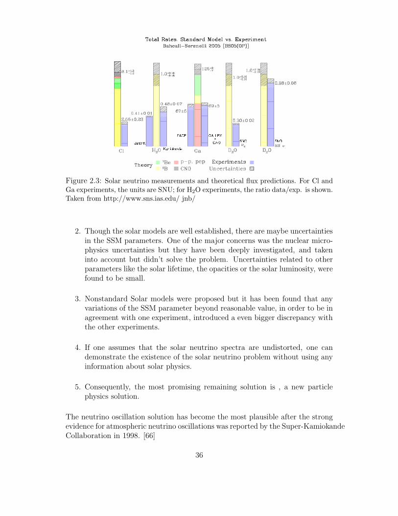
Figure 2.3: Solar neutrino measurements and theoretical flux predictions. For Cl andGa experiments, the units are SNU; for H2O experiments, the ratio data/exp. is shown.Taken from http://www.sns.ias.edu/ jnb/
2. Though the solar models are well established, there are maybe uncertaintiesin the SSM parameters. One of the major concerns was the nuclear micro-physics uncertainties but they have been deeply investigated, and takeninto account but didn’t solve the problem. Uncertainties related to otherparameters like the solar lifetime, the opacities or the solar luminosity, werefound to be small.
3. Nonstandard Solar models were proposed but it has been found that anyvariations of the SSM parameter beyond reasonable value, in order to be inagreement with one experiment, introduced a even bigger discrepancy withthe other experiments.
4. If one assumes that the solar neutrino spectra are undistorted, one candemonstrate the existence of the solar neutrino problem without using anyinformation about solar physics.
5. Consequently, the most promising remaining solution is , a new particlephysics solution.
The neutrino oscillation solution has become the most plausible after the strongevidence for atmospheric neutrino oscillations was reported by the Super-KamiokandeCollaboration in 1998. [66]
36
The Sudbury National Observatroy (SNO) experiment
The Sudbury Neutrino Observatory (SNO) is a neutrino observatory located 6800feet underground6 in Vale Inco’s Creighton Mine in Sudbury, Ontario, Canada.The detector was designed to detect solar neutrinos through their interactionswith a large tank of heavy water surrounded by approximately 9600 photomulti-plier tubes. Unlike previous detectors, using heavy water would make the detectorsensitive to three reactions. In addition to the reaction Eq.(2.3), SNO can detectneutrinos through the charged-current reaction
νe + d→ p+ p+ e−, (2.4)
where the neutrino energy should be at least Emin = 1.44 MeV and the neutralcurrent reaction
νx(νx) + d→ νx(νx) + p+ n (2.5)
which threshold is Emin = 2.23 MeV. The CC reaction (2.4) is very well suited formeasuring the solar neutrino spectrum. Unlike in the case of νae scattering (2.3)in which the energy of incoming neutrino is shared between two light particles inthe final state, the final state of the reaction (2.4) contains only one light particle– electron, and a heavy 2p system whose kinetic energy is very small. There-fore by measuring the electron energy one can directly measure the spectrum ofthe solar neutrinos. The cross section of the NC reaction (2.5) is the same forneutrinos of all three flavours, and therefore oscillations between νe and νµ or ντ
would not change the NC detection rate in the SNO experiment. On the otherhand, these oscillations would deplete the solar νe flux, reducing the CC eventrate. Therefore the CC/NC ratio is a sensitive probe of neutrino flavour oscil-lations. After extensive statistical analysis, it was found that about 35% of thearriving solar neutrinos are electron-neutrinos, with the others being muon- ortau-neutrinos. The total number of detected neutrinos agrees quite well with thepredictions from the SSM [4]. While the Superkamiokande result were not con-clusive about the solar neutrino problem, SNO brought the first direct evidence ofsolar neutrino oscillation in 2001. The solar experiment are suitable to measurea precise mixing angle, but the mass squared difference is better measured onEarth, using electron anti-neutrino flux from nuclear reactors.
The Kamland experiment
The Kamioka Liquid Scintillator Antineutrino Detector (KamLAND) is an ex-periment at the Kamioka Observatory, an underground neutrino observatory nearToyama, Japan. It was built to detect electron anti-neutrino produced by thenuclear powerplants that surround it, and to measure precisely the solar neutrino
6The Creighton mine in Sudbury are among the deepest in the world and therefore presenta very low background radiation.
37
parameters. The scintillator inside the vessel consists of 1,000 tons of mineral oil,benzene and fluorescent chemicals and it is surrounded by 1879 photomultipliertubes mounted on the inner surface. The KamLAND detector not only measuredthe total number of antineutrinos, but also measures their energy. Indeed, theshape of this spectrum carries additional information that can be used to inves-tigate the neutrino oscillation. The spectrum was found to be consistent withneutrino oscillation and a fit provides the values for the ∆m2
12 and θ12 parame-ters. Among three possibilities i.e VO, SMA and LMA [20], Kamland identifiedthe LMA as the solution of the solar neutrino deficit problem. This implies that,as discussed in section 1.2.1, interactions with matter allow them to have anadiabatic resonant conversion via the MSW effect, and through this mechanism,converts greatly into another flavour. This theory was proved thanks to thisexperiment [56]. Since KamLAND measures ∆m2
12 most precisely and the solarexperiments exceed KamLAND’s ability to measure θ12, the most precise oscil-lation parameters are obtained by combining the results from solar experimentsand KamLAND. Such a combined fit gives ∆m2 = (8.0 ± 0.3) × 10−5eV 2 andsin2 2θ12 = 0.86+0.03
−0.04, the best solar neutrino oscillation parameter determinationto date [9]. Nowadays, the only solar running experiments are BOREXINO thatis measuring neutrinos from 7Be [15] and Super-Kamiokande.
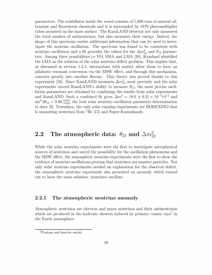
2.2 The atmospheric data: θ23 and ∆m223
While the solar neutrino experiments were the first to investigate astrophysicalsources of neutrinos and unveil the possibility for the oscillation phenomena andthe MSW effect, the atmospheric neutrino experiments were the first to show theevidence of neutrino oscillations proving that neutrinos are massive particles. Notonly solar neutrino experiments needed an explanation for the observed deficit,the atmospheric neutrino experiment also presented an anomaly which turnedout to have the same solution: neutrinos oscillate.
2.2.1 The atmospheric neutrino anomaly
Atmospheric neutrinos are electron and muon neutrinos and their antineutrinoswhich are produced in the hadronic showers induced by primary cosmic rays7 inthe Earth atmosphere.
7Protons and heavier nuclei.
38
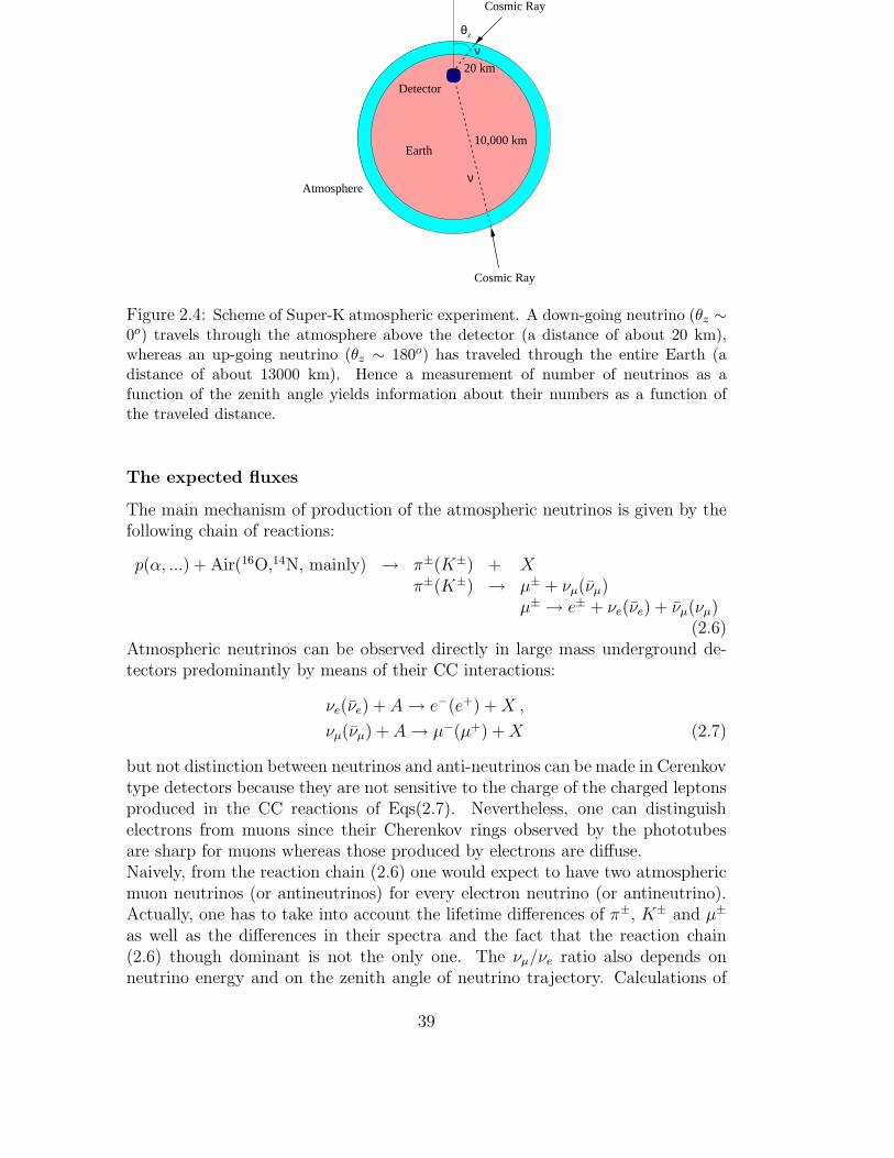
Detector
Earth
Atmosphere
Cosmic Ray
Cosmic Ray
20 km
10,000 km
ν
ν
θz
Figure 2.4: Scheme of Super-K atmospheric experiment. A down-going neutrino (θz ∼0o) travels through the atmosphere above the detector (a distance of about 20 km),whereas an up-going neutrino (θz ∼ 180o) has traveled through the entire Earth (adistance of about 13000 km). Hence a measurement of number of neutrinos as afunction of the zenith angle yields information about their numbers as a function ofthe traveled distance.
The expected fluxes
The main mechanism of production of the atmospheric neutrinos is given by thefollowing chain of reactions:
p(α, ...) + Air(16O,14N, mainly) → π±(K±) + Xπ±(K±) → µ± + νµ(νµ)
µ± → e± + νe(νe) + νµ(νµ)(2.6)
Atmospheric neutrinos can be observed directly in large mass underground de-tectors predominantly by means of their CC interactions:
νe(νe) + A→ e−(e+) +X ,
νµ(νµ) + A→ µ−(µ+) +X (2.7)
but not distinction between neutrinos and anti-neutrinos can be made in Cerenkovtype detectors because they are not sensitive to the charge of the charged leptonsproduced in the CC reactions of Eqs(2.7). Nevertheless, one can distinguishelectrons from muons since their Cherenkov rings observed by the phototubesare sharp for muons whereas those produced by electrons are diffuse.Naively, from the reaction chain (2.6) one would expect to have two atmosphericmuon neutrinos (or antineutrinos) for every electron neutrino (or antineutrino).Actually, one has to take into account the lifetime differences of π±, K± and µ±
as well as the differences in their spectra and the fact that the reaction chain(2.6) though dominant is not the only one. The νµ/νe ratio also depends onneutrino energy and on the zenith angle of neutrino trajectory. Calculations of
39
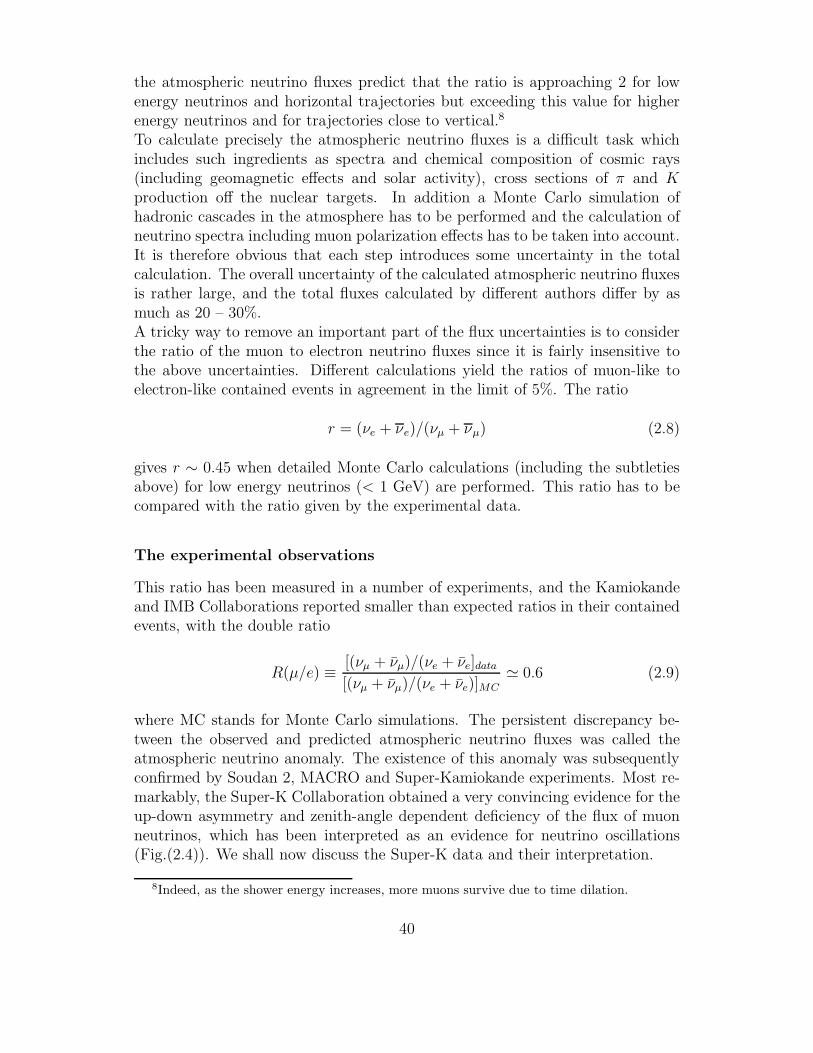
the atmospheric neutrino fluxes predict that the ratio is approaching 2 for lowenergy neutrinos and horizontal trajectories but exceeding this value for higherenergy neutrinos and for trajectories close to vertical.8
To calculate precisely the atmospheric neutrino fluxes is a difficult task whichincludes such ingredients as spectra and chemical composition of cosmic rays(including geomagnetic effects and solar activity), cross sections of π and Kproduction off the nuclear targets. In addition a Monte Carlo simulation ofhadronic cascades in the atmosphere has to be performed and the calculation ofneutrino spectra including muon polarization effects has to be taken into account.It is therefore obvious that each step introduces some uncertainty in the totalcalculation. The overall uncertainty of the calculated atmospheric neutrino fluxesis rather large, and the total fluxes calculated by different authors differ by asmuch as 20 – 30%.A tricky way to remove an important part of the flux uncertainties is to considerthe ratio of the muon to electron neutrino fluxes since it is fairly insensitive tothe above uncertainties. Different calculations yield the ratios of muon-like toelectron-like contained events in agreement in the limit of 5%. The ratio
r = (νe + νe)/(νµ + νµ) (2.8)
gives r ∼ 0.45 when detailed Monte Carlo calculations (including the subtletiesabove) for low energy neutrinos (< 1 GeV) are performed. This ratio has to becompared with the ratio given by the experimental data.
The experimental observations
This ratio has been measured in a number of experiments, and the Kamiokandeand IMB Collaborations reported smaller than expected ratios in their containedevents, with the double ratio
R(µ/e) ≡ [(νµ + νµ)/(νe + νe]data
[(νµ + νµ)/(νe + νe)]MC≃ 0.6 (2.9)
where MC stands for Monte Carlo simulations. The persistent discrepancy be-tween the observed and predicted atmospheric neutrino fluxes was called theatmospheric neutrino anomaly. The existence of this anomaly was subsequentlyconfirmed by Soudan 2, MACRO and Super-Kamiokande experiments. Most re-markably, the Super-K Collaboration obtained a very convincing evidence for theup-down asymmetry and zenith-angle dependent deficiency of the flux of muonneutrinos, which has been interpreted as an evidence for neutrino oscillations(Fig.(2.4)). We shall now discuss the Super-K data and their interpretation.
8Indeed, as the shower energy increases, more muons survive due to time dilation.
40
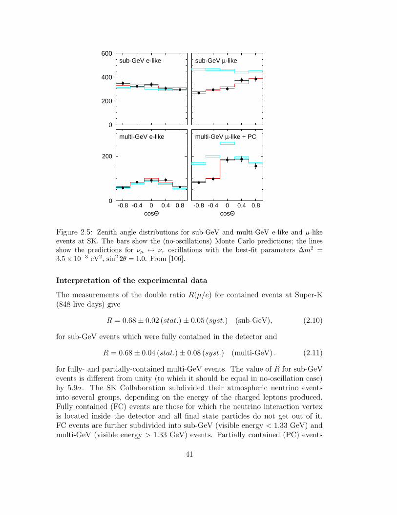
0
200
400
600
-0.8 -0.4 0 0.4 0.80
200
-0.8 -0.4 0 0.4 0.8
sub-GeV e-like sub-GeV µ-like
multi-GeV e-like
cosΘ
multi-GeV µ-like + PC
cosΘ
Figure 2.5: Zenith angle distributions for sub-GeV and multi-GeV e-like and µ-likeevents at SK. The bars show the (no-oscillations) Monte Carlo predictions; the linesshow the predictions for νµ ↔ ντ oscillations with the best-fit parameters ∆m2 =3.5× 10⁻³ eV2, sin2 2θ = 1.0. From [106].
Interpretation of the experimental data
The measurements of the double ratio R(µ/e) for contained events at Super-K(848 live days) give
R = 0.68± 0.02 (stat.)± 0.05 (syst.) (sub-GeV), (2.10)
for sub-GeV events which were fully contained in the detector and
R = 0.68± 0.04 (stat.)± 0.08 (syst.) (multi-GeV) . (2.11)
for fully- and partially-contained multi-GeV events. The value of R for sub-GeVevents is different from unity (to which it should be equal in no-oscillation case)by 5.9σ. The SK Collaboration subdivided their atmospheric neutrino eventsinto several groups, depending on the energy of the charged leptons produced.Fully contained (FC) events are those for which the neutrino interaction vertexis located inside the detector and all final state particles do not get out of it.FC events are further subdivided into sub-GeV (visible energy < 1.33 GeV) andmulti-GeV (visible energy > 1.33 GeV) events. Partially contained (PC) events
41
are those for which the produced muon exits the inner detector volume (onlymuons are penetrating enough).In fig.(2.5) the zenith angle distributions of the SK e-like and µ-like events areshown separately for sub-GeV and multi-GeV contained events. One can see thatfor e-like events, the measured zenith angle distributions agree very well withthe MC predictions (shown by bars), both in the sub-GeV and multi-GeV sam-ples, while for µ-like events both samples show zenith-angle dependent deficiencyof event numbers compared to expectations. The deficit of muon neutrinos isstronger for upward going neutrinos which have larger pathlengths. In the multi-GeV sample, there is practically no deficit of events caused by muon neutrinoscoming from the upper hemisphere (cos θ > 0), whereas in the sub-GeV sample,all µ-like events exhibit a deficit which decreases with cos θ.This pattern is perfectly consistent with oscillations νµ ↔ ντ .
2.2.2 Long-baseline accelerator experiments
The Super-K measurements have been independently confirmed by long base-line experiments: K2K and MINOS. OPERA will also measure the atmosphericoscillation parameters and look for a ντ appearance.
K2K
K2K (KEK to Kamioka) is a long baseline neutrino oscillation experiment us-ing the 12 GeV proton synchrotron accelerator at the High Energy AcceleratorResearch Organization (KEK) in Tsukuba and the Super-Kamiokande detectorwhich lies 250 km away in Kamioka. At KEK site, a νµ neutrino beam is createdand precisely measured by a near detector, therefore predicting the flux numberthat Super-K should measure if neutrino did not oscillate. The disappearance ofνµ seen at Super-K allows to give constraint on the atmospheric parameters [5].
MINOS
MINOS (or Main Injector Neutrino Oscillation Search) is a particle physics ex-periment in which neutrinos produced at Fermilab by the NuMI (Neutrinos atMain Injector) beamline are observed at two detectors, one very close to wherethe beam is produced (the near detector), and another much larger detector 735km away in northern Minnesota (the far detector). Both MINOS detectors havea magnetic field that causes the path of a muon produced in a muon neutrinointeraction to bend, making it possible to separate neutrino and antineutrino in-teractions.
The combined measurements of the atmospheric parameters are at present: sin2(2θ23) >0.92 and ∆m2
32 = 1.9 to 3.0× 10⁻³ eV 2. [9]
42
2.3 The unknown third mixing angle: θ13
Knowing the mixing angle θ13 is of first importance for many reasons, in additionto a deeper knowledge of the MNSP matrix. As it has been said earlier, the CP-violating phase is directly linked to sin θ13, the smaller θ13 is, the more difficultit will be to measure δ. Moreover, θ13 plays a great role in the core-collapsesupernova environment. In fact, what occurs at resonance at high density dependson its value on the one hand and can influence the nucleosynthesis on the otherhand as we will see in the following chapters.
2.3.1 Upper bound for θ13
Since there is no powerful ντ sources available on Earth, neutrino experimental-ists have looked for the disappearance of the electron anti-neutrinos producedby nuclear reactors. The reason why people are looking at anti-neutrinos is sim-ple: nuclear fission reactions produce, via beta-decay, low energy (2-10 MeV)anti-neutrinos with a high precision on the intense emitted flux. Measuring theremaining anti-neutrino flux at a certain distance will give information on theoscillation parameters.Currently, the most stringent constraint on the third mixing angle is given by theCHOOZ experiment. CHOOZ is a little town in France near the France-Belgiumborder where two nuclear reactors of 1450 MW each are present. The CHOOZexperiment is an underground short-baseline reactor-neutrino vacuum-oscillationexperiment which detects electron anti-neutrino by a liquid scintillator calorime-ter located at a distance of about 1 Km from the source. The limit obtainedat 90% level of confidence is: sin2 2θ13 < 0.2 for ∆m2
23 = 2.0 × 10⁻³eV 2 whichcorresponds to θ13 . 9. Improving the upper bound of θ13 is the goal of severalstarting or future experiments. Though not everyone is agreeing on that, somemodels accounts for a value of θ13 close to the current one. There is also indi-cation on the 1 σ level from the combined analysis of experimental results. If itturns out to be true, it will be extremely exciting for the difficult search of theCP-violating phase δ.
2.4 The hierarchy problem
Currently experimental results show that only three flavours of neutrinos areexisting since the LSND results [16, 17] were invalidated by the Mini-Boone ex-periment in 2007 [34]. As we said before, the flavour basis is associated to themass basis composed of three different neutrino masses.
43
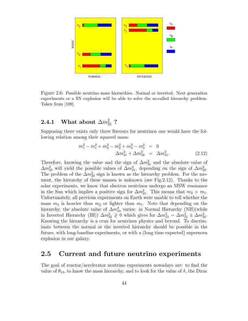
INVERTEDNORMALM
AS
S
3ν
ν2
ν1
ν2ν1
ν3
νe
µν
ντ
Figure 2.6: Possible neutrino mass hierarchies. Normal or inverted. Next generationexperiments or a SN explosion will be able to solve the so-called hierarchy problem.Taken from [109].
2.4.1 What about ∆m231 ?
Supposing there exists only three flavours for neutrinos one would have the fol-lowing relation among their squared mass:
m21 −m2
1 +m22 −m2
2 +m23 −m2
3 = 0
∆m221 + ∆m2
32 = ∆m231. (2.12)
Therefore, knowing the value and the sign of ∆m221 and the absolute value of
∆m223 will yield the possible values of ∆m2
31, depending on the sign of ∆m223.
The problem of the ∆m223 sign is known as the hierarchy problem. For the mo-
ment, the hierarchy of these masses is unknown (see Fig.2.12). Thanks to thesolar experiments, we know that electron neutrinos undergo an MSW resonancein the Sun which implies a positive sign for ∆m2
21. This means that m2 > m1.Unfortunately, all previous experiments on Earth were unable to tell whether themass m3 is heavier than m2 or lighter than m1. Note that depending on thehierarchy, the absolute value of ∆m2
13 varies: in Normal Hierarchy (NH)(whilein Inverted Hierarchy (IH)) ∆m2
32 ≷ 0 which gives for ∆m213 = ∆m2
21 ± ∆m232.
Knowing the hierarchy is a crux for neutrinos physics and beyond. To discrim-inate between the normal or the inverted hierarchy should be possible in thefuture, with long-baseline experiments, or with a (long time expected) supernovaexplosion in our galaxy.
2.5 Current and future neutrino experiments
The goal of reactor/accelerator neutrino experiments nowadays are: to find thevalue of θ13, to know the mass hierarchy, and to look for the value of δ, the Dirac
44
CP-violating phase. Many experiments are on the verge to learn more about θ13.
2.5.1 Current and near-future experiments
The precision on sin2 2θ13 can be improved over previous experiments by: usinglarger detectors to increase statistics, locating the detectors deeper undergroundto suppress background, using ”near” and ”far” detectors to suppress the system-atic uncertainties related to the anti-neutrino flux from reactors. The discoveryof a non-zero θ13 will define the strategy to follow for future accelerator-basedexperiments to measure the value of the Dirac phase.
Double-Chooz
Double-Chooz [13] will improve the Chooz result. This requires an increase inthe statistics, a reduction of the systematic error below one percent, and a care-ful control of the backgrounds. Therefore, Double Chooz will use two identicaldetectors, one at 400 m and another at 1.05 km distance from the Chooz nuclearcores. The plan is to detect the first anti-neutrino before the end of 2009 withone detector and to have both detectors operating by the middle of 2011. Withsuch a scenario Double Chooz will reach a sin2(2θ13) sensitivity of 0.06 after 1year of operation with 1 detector, and 0.03 after 3 years of operation with bothdetectors.
Daya Bay
The Daya Bay Reactor Neutrino Experiment [70] is designed to measure themixing angle θ13 using antineutrinos produced by the reactors of the Daya BayNuclear Power Plant and the Ling Ao Nuclear Power Plant. The goal of the DayaBay experiment is a measurement of sin2(2θ13) to 0.01 or better.
T2K (Tokai to Kamioka)
Contrary to Double-Chooz or Daya Bay which are looking for the disappearanceof electron anti-neutrinos produced by nuclear power plants, the T2K experiment[77] is going to measure the appearance of νe neutrino beam from a νµ beam.The J-PARC facility will produce this intense beam of muon neutrinos directedtowards the Super-Kamiokande detector (295 Km away). Precise measurementsof the other neutrino mixing parameters ∆m2
32 and θ23 are another aim of theexperiment. Future upgrades to T2K could yield measurement of δ by comparingoscillations of neutrinos to those of antineutrinos.
45
Noνa
Intended to be the successor to MINOS, NOνA will consist of two detectors, oneat Fermilab (the near detector), and one in northern Minnesota (the far detector).Neutrinos from NuMI will pass through 810 km of Earth to reach the far detector.NOνA’s main goal is to observe the oscillation of muon to electron neutrinos. If anon-zero value of θ13 is resolvable by the experiment, it will be possible to obtainmeasurements of δ and the mass ordering by also observing the process νµ → νe.
2.5.2 Future long-term experiments
Among the future long-term projects are the Megaton detector experiments andthe experiments designed to measure the hardly reachable CP-violating phase δ.
The Megaton detectors
A series of experimental and theoretical studies are being conducted to assess theastro particle physics potential of future large scale particle detectors as the nextgeneration underground observatories [18]. Three type of detection techniqueshave been proposed all based on the use of large mass of liquid as active media:the liquid argon (like in GLACIER), the liquid scintillator (LENA) and the waterCherenkov (MEMPHYS [46], Hyper Kamiokande, UNO). The purpose for suchmassive detectors, is multidisciplinary and may answer to the still remaining pro-ton decay question. Moreover, their potentiality is enormous in neutrino physics,and more generally in the astro-particle field. It could improve the sensitivityto known neutrino parameters, investigate the solar and atmospheric neutrinomore deeply, look for geoneutrinos, give tremendous information if a supernovaexplosion occur, and even yield information about relic neutrino fluxes. Last butnot least, it would allow the exploration of a very small θ13 and the CP-violationin the leptonic sector, if used in conjunction with future long-term neutrino ac-celerator facilities.
1. Water Cherenkov.
As the cheapest available (active) target material, water is the only liquidthat is realistic for extremely large detectors, up to several hundreds or 1thousand of kton. Water Cherenkov detectors have sufficiently good resolu-tion in energy, position. The technology is well proven, as previously usede.g. in Kamiokande and Super-Kamiokande experiments.
2. Liquid scintillator.
Experiments using a liquid scintillator as active target provide high-energyand angle resolution and offer low-energy threshold. They are particularlyattractive for low energy particle detection, as for example, supernoae, solarneutrinos and geo-neutrinos. Also liquid scintillator detectors exploits a well
46
established technology, already successfully applied at relatively large scalee.g. in Borexino [14, 39] and KamLAND [12] experiments.
3. Liquid Argon.
This detection technology has among the three the best performance inidentifying the topology of interactions and decays of particles, thanks tothe bubble-chamber-like imaging performance. Liquid Argon are very ver-satile and work well with a wide particle energy range.
As mentioned above, the availability of future neutrino beams from particle ac-celerators would provide a supplementary interest axis to the above experiments.Measuring oscillations with artificial neutrinos (of well known kinematical fea-tures) with a sufficiently long baseline would allow to accurately determine theoscillation parameters (in particular the mixing angle θ13 and the CP violatingphase in the mixing matrix). The envisaged detectors may then be used for ob-serving neutrinos from the future Beta Beams and Super Beams in the optimalenergy range for each experiment.
The measurement of δ
There are mainly three type of experiments able to measure very small θ13 valuesand the CP-violating phase: the Beta-Beam, the Super-Beam and the NeutrinoFactory.The Beta-Beam and the neutrino factory exploit new concepts for the productionof neutrino beams while the superbeams are a well established technology. Beta-Beams. Zucchelli has first proposed the idea of producing electron (anti)neutrinobeams using the beta-decay of boosted radioactive ions: the ”beta-beam” [115].It has three main advantages: well-known fluxes, purity (in flavour) and colli-mation. In the original scenario, the ions are produced, collected, accelerated upto several tens GeV/nucleon and stored in a storage ring . The neutrino beamproduced by the decaying ions point to a large water Cerenkov detector about 20times Super-Kamiokande), located at the (upgraded) Frejus Underground Lab-oratory, 130 km away, in order to study CP violation, through a comparison ofνe → νµ and νe → νµ oscillations.
For the two other types, finding δ means to study the CP-violating differenceP (νµ → νe) − P (νµ → νe) between ”neutrino” and ”antineutrino” oscillationprobabilities. To study νµ → νe (νµ → νe) with a super-intense but conven-tionally generated neutrino beam, for example, one would create the beam viathe process π+ → µ+νi (π− → µ−νi), and detect it via νi + target → e− + ...(νi + target → e+ + ...) Depending on the size of θ13, this CP violation maybe observable with a very intense conventional neutrino beam, or may require a”neutrino factory” whose neutrinos come from the decay of stored muons.
47
1. Super-Beams. The first generation of neutrino super-beams, T2K andNOνA, will study the νµ → νe channel which is sensitive to θ13 and δ.The experiments will start by running in neutrino mode. Neutrino run-ning alone, however, implies that the experiments have no sensitivity to δ.A second generation of upgraded superbeams, such as T2HK or the SPL,could follow. The extremely large data sets provided by these experimentswould yield sensitivity to much smaller values of θ13. These experimentscould also search for CP-violation by running with anti-neutrinos, if θ13 islarge enough.
2. Neutrino Factory. The neutrino factory, often called the ultimate neutrinofacility, will be required if θ13 is too small for other facilities to be able tomeasure δ. It will also allow to measure the neutrino hierarchy by exploitingmatter effects in the Earth (see Eq.(1.58)). For these reasons it is consid-ered for many people as the ”ultimate” machine. This last experimentdistinguishes itself by the fact that the detectors will be able to discrimi-nate particles with a positive or a negative charge, and consequently, theneutrinos from the anti-neutrinos.
A a summary for the potentiality of the future neutrino experiments we showthe discovery reach of the various facilities in sin2 2θ13. The figure (2.7) showsthe fraction of all possible values of the true value of the CP phase δ (Fractionof δCP ) for which sin2 2θ13 = 0 can be excluded at the 3σ confidence level asa function of the true value of sin2 2θ13. Of the super-beam facilities, the mostsensitive is the T2HK with the optimised parameter set. The SPL9 super-beamperformance is similar to that of T2HK, while the performance of the WBB10
is slightly worse. While the Beat-Beam seems to be a good option for sin2 2θ13in the range 3.10−3 to 4.10−4, the neutrino factory will be the only option for1.5 10−5 < sin2 2θ13 < 4.10−5. If Nature has decided for θ13 smaller that thisrange astrophysics might play a pivotal role to identify it since one can get uniquefeatures e.g. the supernova time signal if an explosion occur [68] (see chapter 6).
9SPL is a very intense superbeam which could be hosted at CERN.10WBB is the proposal originally put forward by Brookhaven National Laboratory to use
an on-axis, long baseline, wide-band neutrino beam pointed to illuminate a water Cherenkovdetector.
48
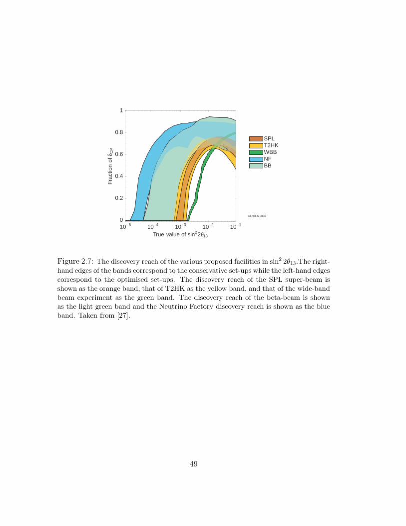
10−5 10−4 10−3 10−2 10−1
True value of sin22θ13
0
0.2
0.4
0.6
0.8
1C
P
SPLT2HKWBBNFBB
GLoBES 2006
Frac
tion
ofδ
Figure 2.7: The discovery reach of the various proposed facilities in sin2 2θ13.The right-hand edges of the bands correspond to the conservative set-ups while the left-hand edgescorrespond to the optimised set-ups. The discovery reach of the SPL super-beam isshown as the orange band, that of T2HK as the yellow band, and that of the wide-bandbeam experiment as the green band. The discovery reach of the beta-beam is shownas the light green band and the Neutrino Factory discovery reach is shown as the blueband. Taken from [27].
49

50
Chapter 3
Neutrinos and core-collapsesupernovae
For massive stars (M ≥ 8M⊙), the end of the stellar evolution process is in-evitably a gigantic explosion known as the supernova, after which the stellar corebecomes either a neutron star or a black hole. During the explosion about 99%of the energy released comes out in the form of neutrinos. This is why neutrinophysicists are so interested in supernovae. In their spectrum, neutrinos carry im-portant information not only about the core-collapse but also about fundamentalproperties of neutrinos, some of them being maybe not explorable in accelera-tors on Earth. The most recent Supernova near our Galaxy was on the 24th ofFebruary 1987, and was detected with neutrino telescope, namely Kamiokande,IMB and Baksan. The Supernova, which emerged from a blue supergiant star,was based in the Large Magellanic Cloud, which is a satellite galaxy of the MilkyWay, at a distance of about 55 Kpc of our solar system. Thanks to the detectionof a few events, the generic features of supernova neutrinos have been roughlyconfirmed, namely that the neutrino signal lasts about 10-12 s, with neutrinoenergies in the several tens of MeV range. These account for practically all thegravitational binding energy released in the process of core collapse. Besides, peo-ple have been able to put limits on neutrino properties such as the time decay,the mass, the magnetic moment or even the electric charge. Here we describe themain features of core-collapse supernova neutrinos and of the supernova modelwe used in our calculations.
51
3.1 General description of core-collapse super-
novae
3.1.1 A qualitative picture
The types of supernovae
For historical reasons, SNe are divided into different types because of their spec-troscopic characteristics near maximum luminosity and by the properties of thelight curve, which depend on the composition of the envelope of the SN progeni-tor star. The two wide categories called type I and type II are characterized bythe absence or presence of hydrogen lines. However, the most important physicalcharacteristic is the mechanism that generates the supernova, which distinguishesSNe of type Ia from SNe of type Ib, Ic and II.We are here interested about the latter type, simply because they produce a hugeflux of neutrinos of all types. These SNe are generated by the collapse of the coreof massive stars (M & 8M⊙), which leaves a compact remnant.Historically, the study of SNe was initiated by W. Baade and F. Zwicky in theearly 1930s. They already suggested that the source of the enormous quantityof energy released in SNe is the gravitational collapse of a star to a neutron starand that SNe may be sources of cosmic rays. In the early 40’s, Gamow andSchoenberg were the first to speculate that neutrino emission would be a majoreffect in the collapse of a star.
The core-collapse mechanism
As stars evolve, like the Sun, they first get their energy burning hydrogen tohelium. The Helium being heavier, settles to the core of the star. The durationof this process depends mainly on the mass of the star. Indeed, the process lastlonger for a less massive star, and shorter for more massive ones. Towards theend of the hydrogen burning period, a period of gravitational contraction heatsup the core and starts the phase of Helium burning to carbon. The carbon beingheavier, will similarly to Helium with hydrogen before, settles to the center withrespectively Helium then Hydrogen floating above. The process of contractionand heating repeats itself towards the end of the helium burning phase whencarbon will start burning to neon. Similar processes then lead from neon tooxygen, and from oxygen to silicon. If a star is more massive than 10 − 11M⊙,silicon burning can start at T ≃ 3.4× 10⁹ K giving rise to iron.At that time, the star has an onion-like structure, with an iron core surrounded byshells composed of elements with decreasing atomic mass. At this point the ironcore has a mass of about 1 solar mass, a radius of a few thousand km, a centraldensity of about 1010 g·cm−3, a central temperature of about 1 MeV, and itsweight is sustained by the pressure of degenerate relativistic electrons. Since iron
52
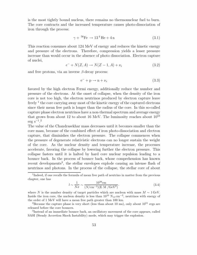
is the most tightly bound nucleus, there remains no thermonuclear fuel to burn.The core contracts and the increased temperature causes photo-dissociation ofiron through the process:
γ + 56Fe → 13 4 He + 4 n (3.1)
This reaction consumes about 124 MeV of energy and reduces the kinetic energyand pressure of the electrons. Therefore, compression yields a lesser pressureincrease than would occur in the absence of photo dissociation. Electron captureof nuclei,
e− +N(Z,A)→ N(Z − 1, A) + νe (3.2)
and free protons, via an inverse β-decay process:
e− + p→ n + νe (3.3)
favored by the high electron Fermi energy, additionally reduce the number andpressure of the electrons. At the onset of collapse, when the density of the ironcore is not too high, the electron neutrinos produced by electron capture leavefreely 1 the core carrying away most of the kinetic energy of the captured electronssince their mean free path is longer than the radius of the core. In this so-calledcapture phase electron neutrinos have a non-thermal spectrum and average energythat grows from about 12 to about 16 MeV. The luminosity reaches about 1053
erg s−1.2
The value of the Chandrasekhar mass decreases until it becomes smaller than thecore mass, because of the combined effect of iron photo-dissociation and electroncapture, that diminishes the electron pressure. The collapse commences whenthe pressure of degenerate relativistic electrons can no longer sustain the weightof the core. As the nuclear density and temperature increase, the processesaccelerate, favoring the collapse by lowering further the electron pressure. Thiscollapse fasters until it is halted by hard core nuclear repulsion leading to abounce back. In the process of bounce back, whose comprehension has knownrecent developments3, the stellar envelopes explode causing an intense flash ofneutrinos and photons. In the process of the collapse, the stellar core of about
1Indeed, if one recalls the formula of mean free path of neutrino in matter from the previouschapter, one has
l ∼ 1
Nσ∼ 1038cm
(N/cm−3)(E M /GeV2). (3.4)
where N is the number density of target particles which are nucleon with mass M ∼ 1 GeV.Inside the iron core, the nucleon density is less than 1010 NA.cm−3, neutrinos with energy ofthe order of 1 MeV will have a mean free path greater than 100 km.
2Because the capture phase is very short (less than about 10 ms), only about 1051 ergs arereleased before the core bounces.
3Instead of an immediate bounce back, an oscillatory movement of the core appears, calledSASI (Steady Accretion Shock Instability) mode, which may trigger the explosion.
53
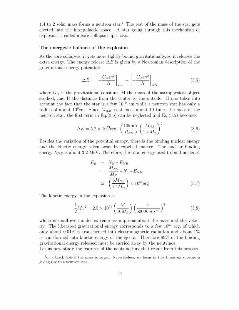
1.4 to 2 solar mass forms a neutron star.4 The rest of the mass of the star getsejected into the intergalactic space. A star going through this mechanism ofexplosion is called a core-collapse supernova.
The energetic balance of the explosion
As the core collapses, it gets more tightly bound gravitationally, so it releases theextra energy. The energy release ∆E is given by a Newtonian description of thegravitational energy potential:
∆E =
[
−GNm2
R
]
star
−[
−GNm2
R
]
NS
(3.5)
where GN is the gravitational constant, M the mass of the astrophysical objectstudied, and R the distance from the center to the outside. If one takes intoaccount the fact that the star is a few 1010 cm while a neutron star has only aradius of about 106cm. Since Mstar is at most about 10 times the mass of theneutron star, the first term in Eq.(3.5) can be neglected and Eq.(3.5) becomes:
∆E = 5.2× 1053erg ·(
10km
RNS
)(
MNS
1.4M⊙
)2
(3.6)
Besides the variation of the potential energy, there is the binding nuclear energyand the kinetic energy taken away by expelled matter. The nuclear bindingenergy ENB is about 3.2 MeV. Therefore, the total energy used to bind nuclei is:
EB = NN ∗ ENB
=MNS
MN∗Na ∗ ENB
≃(
6MNS
1.4M⊙
)
× 1051erg (3.7)
The kinetic energy in the explosion is
1
2Mv2 = 2.5× 1051
(
M
10M⊙
)
( v
5000km.s−1
)2
(3.8)
which is small even under extreme assumptions about the mass and the veloc-ity. The liberated gravitational energy corresponds to a few 1053 erg, of whichonly about 0.01% is transformed into electromagnetic radiation and about 1%is transformed into kinetic energy of the ejecta. Therefore 99% of the bindinggravitational energy released must be carried away by the neutrinos.Let us now study the features of the neutrino flux that result from this process.
4or a black hole if the mass is larger. Nevertheless, we focus in this thesis on supernovagiving rise to a neutron star.
54
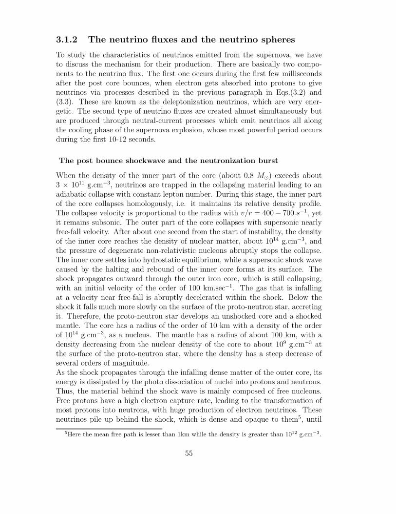
3.1.2 The neutrino fluxes and the neutrino spheres
To study the characteristics of neutrinos emitted from the supernova, we haveto discuss the mechanism for their production. There are basically two compo-nents to the neutrino flux. The first one occurs during the first few millisecondsafter the post core bounces, when electron gets absorbed into protons to giveneutrinos via processes described in the previous paragraph in Eqs.(3.2) and(3.3). These are known as the deleptonization neutrinos, which are very ener-getic. The second type of neutrino fluxes are created almost simultaneously butare produced through neutral-current processes which emit neutrinos all alongthe cooling phase of the supernova explosion, whose most powerful period occursduring the first 10-12 seconds.
The post bounce shockwave and the neutronization burst
When the density of the inner part of the core (about 0.8 M⊙) exceeds about3 × 1011 g.cm−3, neutrinos are trapped in the collapsing material leading to anadiabatic collapse with constant lepton number. During this stage, the inner partof the core collapses homologously, i.e. it maintains its relative density profile.The collapse velocity is proportional to the radius with v/r = 400− 700.s−1, yetit remains subsonic. The outer part of the core collapses with supersonic nearlyfree-fall velocity. After about one second from the start of instability, the densityof the inner core reaches the density of nuclear matter, about 1014 g.cm−3, andthe pressure of degenerate non-relativistic nucleons abruptly stops the collapse.The inner core settles into hydrostatic equilibrium, while a supersonic shock wavecaused by the halting and rebound of the inner core forms at its surface. Theshock propagates outward through the outer iron core, which is still collapsing,with an initial velocity of the order of 100 km.sec−1. The gas that is infallingat a velocity near free-fall is abruptly decelerated within the shock. Below theshock it falls much more slowly on the surface of the proto-neutron star, accretingit. Therefore, the proto-neutron star develops an unshocked core and a shockedmantle. The core has a radius of the order of 10 km with a density of the orderof 1014 g.cm−3, as a nucleus. The mantle has a radius of about 100 km, with adensity decreasing from the nuclear density of the core to about 109 g.cm−3 atthe surface of the proto-neutron star, where the density has a steep decrease ofseveral orders of magnitude.As the shock propagates through the infalling dense matter of the outer core, itsenergy is dissipated by the photo dissociation of nuclei into protons and neutrons.Thus, the material behind the shock wave is mainly composed of free nucleons.Free protons have a high electron capture rate, leading to the transformation ofmost protons into neutrons, with huge production of electron neutrinos. Theseneutrinos pile up behind the shock, which is dense and opaque to them5, until
5Here the mean free path is lesser than 1km while the density is greater than 1012 g.cm−3.
55
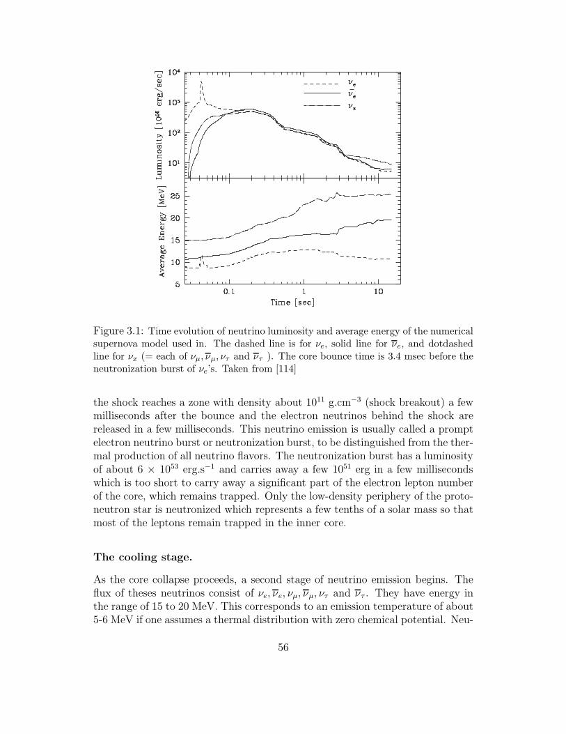
Figure 3.1: Time evolution of neutrino luminosity and average energy of the numericalsupernova model used in. The dashed line is for νe, solid line for νe, and dotdashedline for νx (= each of νµ, νµ, ντ and ντ ). The core bounce time is 3.4 msec before theneutronization burst of νe’s. Taken from [114]
the shock reaches a zone with density about 1011 g.cm−3 (shock breakout) a fewmilliseconds after the bounce and the electron neutrinos behind the shock arereleased in a few milliseconds. This neutrino emission is usually called a promptelectron neutrino burst or neutronization burst, to be distinguished from the ther-mal production of all neutrino flavors. The neutronization burst has a luminosityof about 6 × 1053 erg.s−1 and carries away a few 1051 erg in a few millisecondswhich is too short to carry away a significant part of the electron lepton numberof the core, which remains trapped. Only the low-density periphery of the proto-neutron star is neutronized which represents a few tenths of a solar mass so thatmost of the leptons remain trapped in the inner core.
The cooling stage.
As the core collapse proceeds, a second stage of neutrino emission begins. Theflux of theses neutrinos consist of νe, νe, νµ, νµ, ντ and ντ . They have energy inthe range of 15 to 20 MeV. This corresponds to an emission temperature of about5-6 MeV if one assumes a thermal distribution with zero chemical potential. Neu-
56
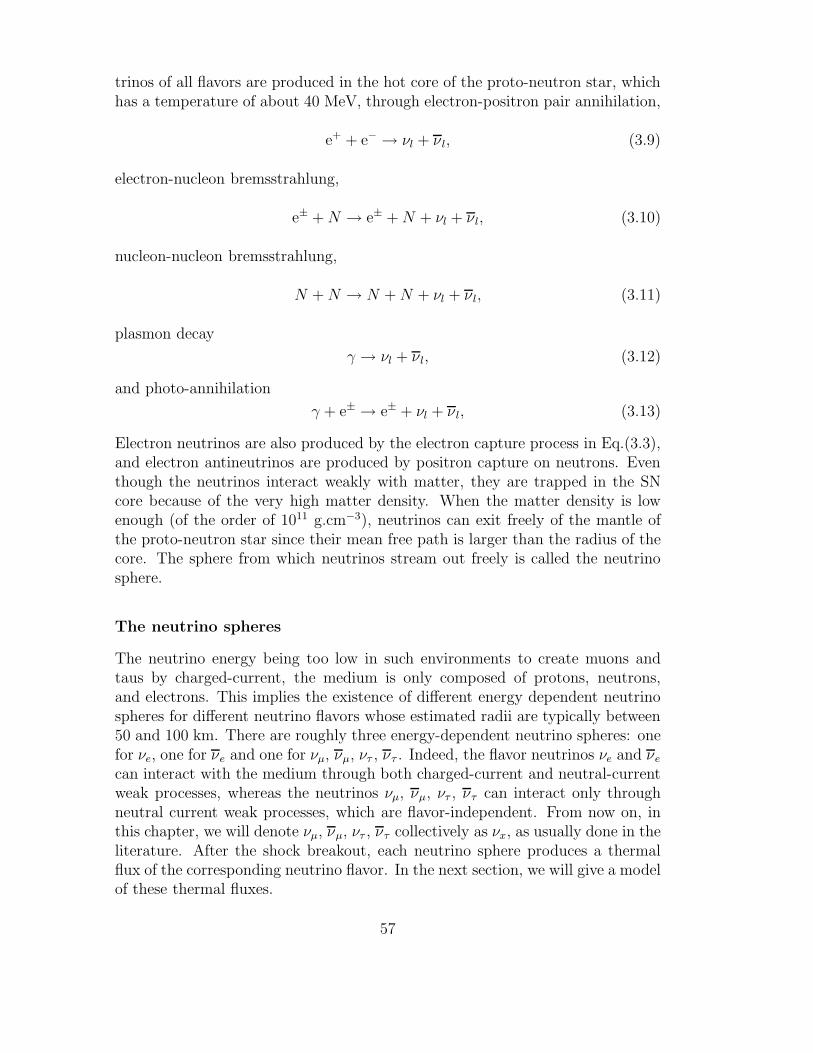
trinos of all flavors are produced in the hot core of the proto-neutron star, whichhas a temperature of about 40 MeV, through electron-positron pair annihilation,
e+ + e− → νl + ν l, (3.9)
electron-nucleon bremsstrahlung,
e± +N → e± +N + νl + νl, (3.10)
nucleon-nucleon bremsstrahlung,
N +N → N +N + νl + ν l, (3.11)
plasmon decay
γ → νl + νl, (3.12)
and photo-annihilation
γ + e± → e± + νl + ν l, (3.13)
Electron neutrinos are also produced by the electron capture process in Eq.(3.3),and electron antineutrinos are produced by positron capture on neutrons. Eventhough the neutrinos interact weakly with matter, they are trapped in the SNcore because of the very high matter density. When the matter density is lowenough (of the order of 1011 g.cm−3), neutrinos can exit freely of the mantle ofthe proto-neutron star since their mean free path is larger than the radius of thecore. The sphere from which neutrinos stream out freely is called the neutrinosphere.
The neutrino spheres
The neutrino energy being too low in such environments to create muons andtaus by charged-current, the medium is only composed of protons, neutrons,and electrons. This implies the existence of different energy dependent neutrinospheres for different neutrino flavors whose estimated radii are typically between50 and 100 km. There are roughly three energy-dependent neutrino spheres: onefor νe, one for νe and one for νµ, νµ, ντ , ντ . Indeed, the flavor neutrinos νe and νe
can interact with the medium through both charged-current and neutral-currentweak processes, whereas the neutrinos νµ, νµ, ντ , ντ can interact only throughneutral current weak processes, which are flavor-independent. From now on, inthis chapter, we will denote νµ, νµ, ντ , ντ collectively as νx, as usually done in theliterature. After the shock breakout, each neutrino sphere produces a thermalflux of the corresponding neutrino flavor. In the next section, we will give a modelof these thermal fluxes.
57
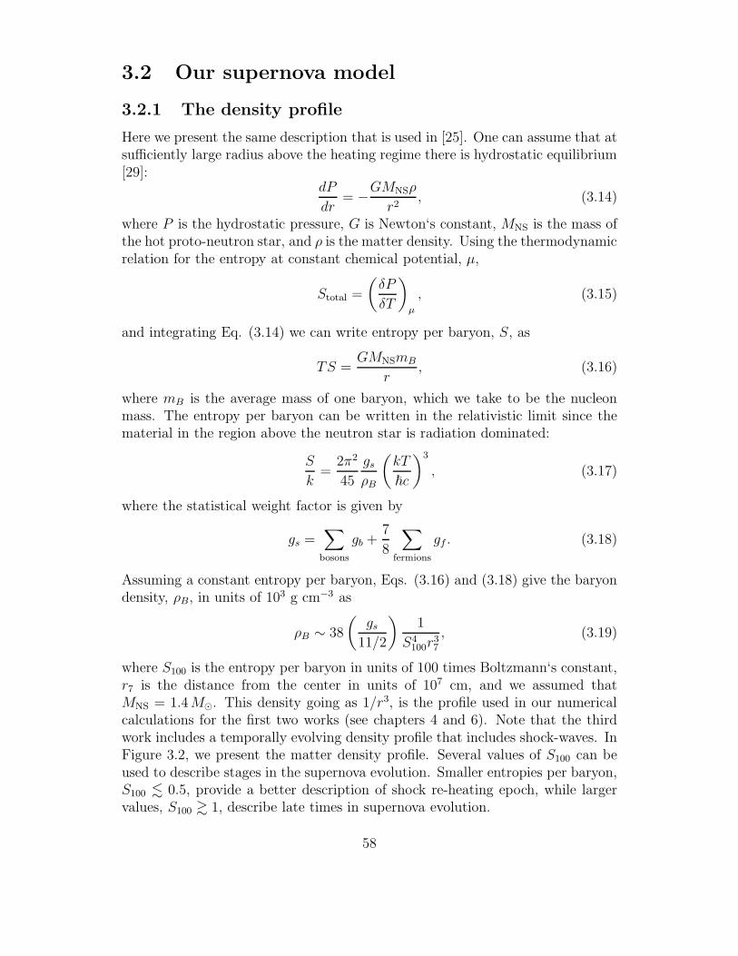
3.2 Our supernova model
3.2.1 The density profile
Here we present the same description that is used in [25]. One can assume that atsufficiently large radius above the heating regime there is hydrostatic equilibrium[29]:
dP
dr= −GMNSρ
r2, (3.14)
where P is the hydrostatic pressure, G is Newton‘s constant, MNS is the mass ofthe hot proto-neutron star, and ρ is the matter density. Using the thermodynamicrelation for the entropy at constant chemical potential, µ,
Stotal =
(
δP
δT
)
µ
, (3.15)
and integrating Eq. (3.14) we can write entropy per baryon, S, as
TS =GMNSmB
r, (3.16)
where mB is the average mass of one baryon, which we take to be the nucleonmass. The entropy per baryon can be written in the relativistic limit since thematerial in the region above the neutron star is radiation dominated:
S
k=
2π2
45
gs
ρB
(
kT
~c
)3
, (3.17)
where the statistical weight factor is given by
gs =∑
bosons
gb +7
8
∑
fermions
gf . (3.18)
Assuming a constant entropy per baryon, Eqs. (3.16) and (3.18) give the baryondensity, ρB, in units of 103 g cm−3 as
ρB ∼ 38
(
gs
11/2
)
1
S4100r
37
, (3.19)
where S100 is the entropy per baryon in units of 100 times Boltzmann‘s constant,r7 is the distance from the center in units of 107 cm, and we assumed thatMNS = 1.4M⊙. This density going as 1/r3, is the profile used in our numericalcalculations for the first two works (see chapters 4 and 6). Note that the thirdwork includes a temporally evolving density profile that includes shock-waves. InFigure 3.2, we present the matter density profile. Several values of S100 can beused to describe stages in the supernova evolution. Smaller entropies per baryon,S100 . 0.5, provide a better description of shock re-heating epoch, while largervalues, S100 & 1, describe late times in supernova evolution.
58
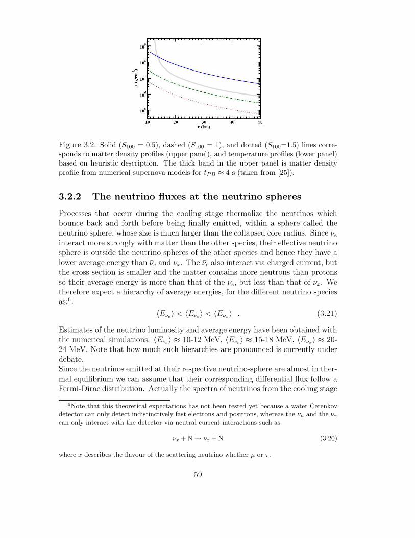
Figure 3.2: Solid (S100 = 0.5), dashed (S100 = 1), and dotted (S100=1.5) lines corre-sponds to matter density profiles (upper panel), and temperature profiles (lower panel)based on heuristic description. The thick band in the upper panel is matter densityprofile from numerical supernova models for tPB ≈ 4 s (taken from [25]).
3.2.2 The neutrino fluxes at the neutrino spheres
Processes that occur during the cooling stage thermalize the neutrinos whichbounce back and forth before being finally emitted, within a sphere called theneutrino sphere, whose size is much larger than the collapsed core radius. Since νe
interact more strongly with matter than the other species, their effective neutrinosphere is outside the neutrino spheres of the other species and hence they have alower average energy than νe and νx. The νe also interact via charged current, butthe cross section is smaller and the matter contains more neutrons than protonsso their average energy is more than that of the νe, but less than that of νx. Wetherefore expect a hierarchy of average energies, for the different neutrino speciesas:6.
〈Eνe〉 < 〈Eνe
〉 < 〈Eνx〉 . (3.21)
Estimates of the neutrino luminosity and average energy have been obtained withthe numerical simulations: 〈Eνe
〉 ≈ 10-12 MeV, 〈Eνe〉 ≈ 15-18 MeV, 〈Eνx
〉 ≈ 20-24 MeV. Note that how much such hierarchies are pronounced is currently underdebate.Since the neutrinos emitted at their respective neutrino-sphere are almost in ther-mal equilibrium we can assume that their corresponding differential flux follow aFermi-Dirac distribution. Actually the spectra of neutrinos from the cooling stage
6Note that this theoretical expectations has not been tested yet because a water Cerenkovdetector can only detect indistinctively fast electrons and positrons, whereas the νµ and the ντ
can only interact with the detector via neutral current interactions such as
νx + N→ νx + N (3.20)
where x describes the flavour of the scattering neutrino whether µ or τ .
59
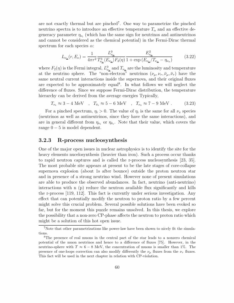
are not exactly thermal but are pinched7. One way to parametrize the pinchedneutrino spectra is to introduce an effective temperature Tα and an effective de-generacy parameter ηνi
(which has the same sign for neutrinos and antineutrinosand cannot be considered as the chemical potential) in the Fermi-Dirac thermalspectrum for each species α:
Lνα(r, Eν) =
1
4πr2
L0να
T 3να〈Eνα〉F2(η)
E2να
1 + exp (Eνα/Tνα
− ηνα)
(3.22)
where F2(η) is the Fermi integral, L0να
and Tναare the luminosity and temperature
at the neutrino sphere. The “non-electron” neutrinos (νµ, ντ , νµ, ντ ) have thesame neutral current interactions inside the supernova, and their original fluxesare expected to be approximately equal8. In what follows we will neglect thedifference of fluxes. Since we suppose Fermi-Dirac distribution, the temperaturehierarchy can be derived from the average energies Typically,
Tνe≈ 3− 4 MeV , Tνe
≈ 5− 6 MeV , Tνx≈ 7− 9 MeV . (3.23)
For a pinched spectrum, ηi > 0. The value of ηi is the same for all νx species(neutrinos as well as antineutrinos, since they have the same interactions), andare in general different from ηνe
or ηνe. Note that their value, which covers the
range 0− 5 is model dependent.
3.2.3 R-process nucleosynthesis
One of the major open issues in nuclear astrophysics is to identify the site for theheavy elements nucelosynthesis (heavier than iron). Such a process occur thanksto rapid neutron captures and is called the r-process nucleosynthesis [23, 35].The most probable site appears at present to be the late stages of core-collapsesupernova explosion (about 1s after bounce) outside the proton neutron starand in presence of a strong neutrino wind. However none of present simulationsare able to produce the observed abundances. In fact, neutrino (anti-neutrino)interactions with n (p) reduce the neutron available flux significantly and killsthe r-process [119, 112]. This fact is currently under serious investigation. Anyeffect that can potentially modify the neutron to proton ratio by a few percentmight solve this crucial problem. Several possible solutions have been evoked sofar, but for the moment this puzzle remains unsolved. In this thesis, we explorethe possibility that a non-zero CP-phase affects the neutron to proton ratio whichmight be a solution of this hot open issue.
7Note that other parametrizations like power-law have been shown to nicely fit the simula-tions.
8The presence of real muons in the central part of the star leads to a nonzero chemicalpotential of the muon neutrinos and hence to a difference of fluxes [75]. However, in theneutrino-sphere with T ≈ 6 − 8 MeV, the concentration of muons is smaller than 1%. Thepresence of one-loops correction can also modify differently the νµ fluxes from the ντ fluxes.This fact will be used in the next chapter in relation with CP-violation.
60
0 20 40 60 80 Neutrino Energy (MeV)
2e+12
4e+12
6e+12
8e+12
1e+13
Lum
inos
ity
(a.
u.)
Figure 3.3: Neutrino fluxes at the neutrinosphere: the curves show the Fermi-Dirac distributions used for electron neutrinos with Tνe
= 3.2 MeV (solid), elec-tron anti-neutrinos Tνe
= 4.8 MeV (dashed) and for the other flavors Tνx= 7.6
MeV (with νx = νµ, ντ , νµ, ντ ) (dotted line).
Reaction Rates
As seen earlier, the dominant reactions that control the n/p ratio is the capturereactions on free nucleons
νe + n p + e−, (3.24)
and
νe + p n + e+. (3.25)
In our calculation [26] (see chapter 5) we took a simplified formula 9 for thereaction cross sections, namely [100]
σνe(Eνe
) ≈ 9.6× 10−44
(
Eνe+ ∆np
MeV
)2
cm2, (3.26)
and
σνe(Eνe
) ≈ 9.6× 10−44
(
Eνe−∆np
MeV
)2
cm2, (3.27)
where ∆np ≈ 1.293 MeV is the neutron proton mass difference. The associatedrates can be written as [67]
λ =
∫
σ(E)νdLν
dEνdEν . (3.28)
9Such cross sections can also be computed numerically exactly. For simplicity we ignoredweak magnetism and recoil corrections, which may be important [76].
61
with Lν given by Eq.(3.22). Introducing Nj , number of species of kind j per unitvolume, the rate of change of the number of protons can be expressed as
dNp
dt= −(λνe
+ λe−)Np + (λνe+ λe+)Nn, (3.29)
where λνeand λe− are the rates of the forward and backward reactions in Eq.(3.24)
and λνeand λe+ are the rates of the forward and backward reactions in Eq.(3.25).
The electron fraction in the media
The electron fraction, Ye, is the net number of electrons (number of electronsminus the number of positrons) per baryon:
Ye = (ne− − ne+)/nB, (3.30)
where ne− , ne+ , and nB are number densities of electrons, positrons, and baryons,respectively. Defining Aj , the atomic weight of the j-th species, one can writedown expressions for the mass fraction, Xj
Xj =NjAj∑
iNiAi, (3.31)
and the number abundance relative to baryons, Yj,
Yj =Xj
Aj=
Nj∑
iNiAi. (3.32)
The electron fraction defined in Eq. (3.30) can then be rewritten as
Ye =∑
i
ZiYi =∑
i
(
Zi
Ai
)
Xi
= Xp +1
2Xα, (3.33)
where Zi is the charge of the species of kind i, and the mass fractions of protons,Xp, alpha particles, Xα. We assume here that no heavy nuclei are present in themedium. Since the quantity
∑
iNiAi does not change with neutrino interactions,one can rewrite Eq.(3.29) in terms of mass fractions
dXp
dt= −(λνe
+ λe−)Xp + (λνe+ λe+)Xn. (3.34)
Because of the very large binding energy, the rate of alpha particle interactionswith neutrinos is nearly zero and we can write dYe/dt = dXp/dt. Using theconstraint Xp +Xn +Xα = 1, Eq.(3.34) can be rewritten as
dYe
dt= λn − (λp + λn)Ye +
1
2(λp − λn)Xα, (3.35)
62
where we introduced the total proton loss rate λp = λνe+ λe− and the total
neutron loss rate λn = λνe+ λe+ . It has been shown that when the rates of
these processes are rapid as compared to the outflow rate a “weak chemicalequilibrium” is established [99]. The weak freeze-out radius is defined to bewhere the neutron-to-proton conversion rate is less than the outflow rate of thematerial. If the plasma reaches a weak equilibrium stage then Ye is no longerchanging: dYe/dt = 0. From Eq.(3.35) one can write the equilibrium value of theelectron fraction
Ye =λn
λp + λn+
1
2
λp − λn
λp + λnXα. (3.36)
At high temperatures alpha particles are absent and the second term in Eq.(3.36)can be dropped10. In the region just below where the alpha particles are formedapproximately one second after the bounce, the temperature is less then ∼ 1MeV. Here both the electron and positron capture rates are very small and Ye
can be approximated as
Y (0)e =
1
1 + λνe/λνe
. (3.37)
Using Eq. (3.32), we rewrite Eq. (3.37):
Y (0)e (r) =
(
1 +
∫∞0σνe
(E)dLνe (r,E)dE
dE∫∞0σνe
(E)dLνe (r,E)dE
dE
)−1
. (3.38)
This is the formula we use in our numerical simulations (see chapters 4 and6). Neutrino oscillations, since they can swap energies of different flavors, canaffect the energy-dependent rates in Eqs.(3.37) and (3.38), changing the electronfraction. In the next chapter, we will show how CP-violation effects may impactthe electron neutrino and anti-neutrino fluxes, and consequently the electronfraction.
10At lower temperature the alpha particle mass fraction increases. Consequently free nucleonsget bound in alphas and cease interacting with neutrinos, because of the large binding energyof the alpha particle. This phenomenon is called ”alpha effect”, it can increases the value of Ye
which implies fewer free neutrons, and therefore negatively impacts r-process nucleosynthesis[118]. We do not consider the alpha effect in our numerical simulation, a future work shouldinclude it.
63

64
Part III
Neutrino properties andsupernovae
65

Chapter 4
CP-violation and supernovaneutrinos
One of the crucial open issues in neutrino physics is the possible existence of CPviolation in the lepton sector. Indeed, if the remaining mixing angle θ13 is rela-tively large there is a possibility that violation of CP symmetry may be observablein the neutrino sector. Among others, the discovery of a non-zero Dirac deltaphase might help our understanding of the observed matter-antimatter asymme-try of the universe. A vast literature exists on possible studies with terrestrialexperiments using man-made sources. Only a few recent works have addressedthe possible measurement of the CP-violating phase with neutrinos from astro-physical sources. The paper by Winter [116] uses astrophysical sources to learnabout the leptonic CP phase, and it focusses on high energy neutrinos only. Thepurpose of the first work of this thesis [26] is to explore possible effects comingfrom the CP-violating phase in dense matter, such in core collapse supernovae.Several supernova observables can be in theory affected by this phase, such as theneutrino fluxes, inside and outside the star, and also the r-process nucleosynthesisvia the electron fraction. We first analyze analytically and in general terms, howthe neutrino propagation equations and the evolution operator are modified inmatter, in presence of a non-zero Dirac delta phase. We then discuss possibleeffects induced by the Dirac CP-violating phase on two particular observablesin the core-collapse supernova environment: the neutrino fluxes and the electronfraction Ye.
67
4.1 CP effects with neutrino interactions at tree
level
4.1.1 Exact analytical formulas
In this section, our aim is simple: try to obtain relations on the oscillatingprobabilities in matter at tree level, showing explicit dependence of the DiracCP-violating phase δ. All along this section we work with neutrinos but thederivation and the implications would be exactly the same for anti-neutrinos.
The factorization
To do so, we start naturally with the evolution equation of neutrinos in matterwithin the wave functions formalism. In three flavours, the MSW equation (1.44)is
i∂
∂t
Ψe
Ψµ
Ψτ
=
T23T13T12
E1 0 00 E2 00 0 E3
T †12T
†13T
†23 +
Vc + Vn 0 00 Vn 00 0 Vn
Ψe
Ψµ
Ψτ
,
(4.1)where T23T13T12 accounts for the MNSP matrix U , and their definition is
T12 =
c12 s12 0−s12 c12 0
0 0 1
, T13 =
c13 0 s13 e−iδ
0 1 0−s13 e
iδ 0 c13
, T23 =
1 0 00 c23 s23
0 −s23 c23
,
(4.2)We remind that
Vc(x) =√
2GFNe(x) (4.3)
for the charged-current and
Vn(x) = − 1√2GFNn(x). (4.4)
for the neutral current. Since Vn only contributes an overall phase to the neutrinoevolution we ignore it. For now we ignore any corrections to the interactionsbetween neutrinos and matter beyond tree-level. We also do not consider herethe neutrino-neutrino interactions. Such additional interactions will be discussedin section (4.2) and chapter 5 and 6 respectively. Our goal is to make the phaseδ explicitly appear. This phase is contained in the T13 rotation matrix and canbe factorized easily to yield the relation:
T13 = S T 013 S
† (4.5)
68
where S(δ) = diag(1, 1, eiδ)1. Since S does not commute with the rotation matrixT23, we have to work with rotated wave functions written in another basis thatwe call the T23 basis. We therefore introduce the combinations
Ψµ = cos θ23Ψµ − sin θ23Ψτ , (4.6)
Ψτ = sin θ23Ψµ + cos θ23Ψτ . (4.7)
This corresponds to multiplying the neutrino column vector in Eq. (4.1) with T †23
from the left. Eq. (4.1) then becomes
i∂
∂t
Ψe
Ψµ
Ψτ
=
ST 013T12
E1 0 00 E2 00 0 E3
T †12T
013
†S† +
Vc 0 00 0 00 0 0
Ψe
Ψµ
Ψτ
,
(4.8)since S commute with T12 and of course diag(E1, E2, E3). It is easy to noticethat the S matrix commutes with the matter term of the total Hamiltonian thatwe call H in this basis. The Hamiltonian H depends on the CP-violating phase,δ via the formula
H(δ) = S H(δ = 0)S†. (4.9)
We now know that the explicit dependence of δ can be factorized out of theHamiltonian in that particular basis. To see the consequence of such a factor-ization, it is more interesting to work with the transition amplitudes that arepresent in the evolution operator formalism (See appendix C for details.). Weare interested in solving the evolution equation corresponding to Eq.(4.8):
i~dU(δ)
dt= H(δ)U(δ). (4.10)
It is important to recall that we need to solve this equation with the initialcondition
U(δ)(t = 0) = 1. (4.11)
DefiningU0 = S†U(δ), (4.12)
and using the relation in Eq.(4.9) we get
i~dU0
dt= H(δ = 0) U0, (4.13)
i.e. U0 provides the evolution when the CP-violating phase is set to zero. UsingEq.(4.11) we see that the correct initial condition on U0 is U0(t = 0) = S†.However, Eq.(4.13) is nothing but the neutrino evolution equation with the CP-violating phase set equal to zero. If we call the solution of this equation with the
1From this formula we have the straightforward but useful relation T †13 = S T 0
13†S†.
69
standard initial condition U(δ = 0)(t = 0) = 1 to be U(δ = 0), we see that weshould set U0 = U(δ = 0)S†, which yields
U(δ) = S U(δ = 0)S†. (4.14)
This relation can also be obtained by a simpler but equivalent derivation.If we consider Eq.(4.10) respectively in the case where δ = 0 and the case whereδ 6= 0:
i~dU(δ = 0)
dt= H(δ = 0) U(δ = 0). (4.15)
and
i~dU(δ)
dt= H(δ) U(δ). (4.16)
We use the relation Eq.(4.9) and multiplied each side of the equation by the Smatrix to obtain:
i~d S† U(δ)S
dt= H(δ)S† U(δ)S. (4.17)
We then take the difference between Eq.(4.16) and Eq.(4.15) multiplied by S, wehave:
i~d
dt
(
S† U(δ)S − U(δ = 0))
= H(δ = 0)(
S† U(δ)S − U(δ = 0))
. (4.18)
that we can rewrite:
i~d
dt(∆(δ)) = H(δ = 0) (∆(δ)) . (4.19)
Therefore, realizing that S† U(δ)S has the same initial condition that U(δ = 0),the variable ∆ which is a priori a function of δ is zero initially. By recurrencethe variable ∆ will remain zero and therefore we find of Eq.(4.14). This equationillustrates how the effects of the CP-violating phase separate in describing theneutrino evolution. It is valid both in vacuum and in matter for any densityprofile. It is easy to verify that this result does not depend on the choice of theparametrization for the neutrino mixing matrix.
The transition probabilities and the CP-violating phase
The solution of Eq. (4.16) can also be written in the form:
U(δ) =
Aee Aµe Aτ e
Aeµ Aµµ Aτ µ
Aeτ Aµτ Aτ τ
. (4.20)
70
where the quantity Axy is the amplitude of the oscillation from νx to νy when δis non-zero. Similarly we define the amplitude for the process νx → νy to be Bxy
when δ = 0 so thatP (νx → νy, δ 6= 0) = |Axy|2. (4.21)
andP (νx → νy, δ = 0) = |Bxy|2. (4.22)
Using Eq. (4.14) it is possible to relate survival probabilities for the two caseswith δ = 0 and δ 6= 0. These solutions will be related as
Aee Aµe Aτ e
Aeµ Aµµ Aτ µ
Aeτ Aµτ Aτ τ
=
1 0 00 1 00 0 eiδ
Bee Bµe Bτ e
Beµ Bµµ Bτ µ
Beτ Bµτ Bτ τ
1 0 00 1 00 0 e−iδ
(4.23)One can immediately see that the electron neutrino survival probability does notdepend on the CP-violating phase, as in vacuum,
Aee = Bee (4.24)
which implies:P (νe → νe, δ 6= 0) = P (νe → νe, δ = 0). (4.25)
One can further write
c23Aµe − s23Aτe = c23Bµe − s23Bτe
s23Aµe + c23Aτe = e−iδ[s23Bµe + c23Bτe]
By solving these equations one gets
Aµe = (c223 + s223e
−iδ)Bµe + c23s23(e−iδ − 1)Bτe, (4.26)
andAτe = c23s23(e
−iδ − 1)Bµe + (s223 + c223e
−iδ)Bτe. (4.27)
Clearly the individual amplitudes in Eqs.(4.26) and (4.27) depend on the CP-violating phase. However, taking absolute value squares of Eqs.(4.26) and (4.27),after some algebra, one obtains:
|Aµe|2 + |Aτe|2 = |Bµe|2 + |Bτe|2, (4.28)
or equivalently
P (νµ → νe, δ 6= 0) + P (ντ → νe, δ 6= 0) = P (νµ → νe, δ = 0) + P (ντ → νe, δ = 0).(4.29)
This relation could also be immediately obtained by the relation of conservationof probability
P (νe → νe) + P (νµ → νe) + P (ντ → νe) = 1 (4.30)
which comes from the unitarity of the evolution operator.
71
Implications on the fluxes in the supernova environment
According to supernova simulations, the neutrino fluxes at the neutrino sphereare quite well described by Fermi-Dirac distributions or power-law spectra [78].Neutrino masses and mixings modify this simple pattern by mixing the spectraduring neutrino evolution. We recall that a neutrino hierarchy of temperaturesat the neutrino sphere exists Eq.(3.21). The (differential) neutrino fluxes of typei (mass or flavour) are given logically by this formula:
φνi(δ) = Lνi
P (νi → νi) + LνjP (νj → νi) + Lνk
P (νk → νi) (4.31)
where the luminosities are defined by the following relation:
Lνi(r, Eν) =
L0νi
4πr2(Tνi)3
1
〈Eν〉F2(η)
E2ν
1 + exp (Eν/Tν − ηνi)
(4.32)
as seen in chapter 3.Since here we consider interactions between neutrinos and matter only at tree
level, the interactions via neutral current for νµ and ντ will be the same beforebeing emitted at the neutrino-sphere. Their respective last scattering surface willalso be superimposed with such assumptions. Consequently, for νµ and ντ we havethe same L0
νi, the same temperature Tνi
(therefore the same average energy) andfinally the same pinched factor ηνi
. All these equalities on the different parametersof a flux (Eq.(4.32)) imply the equality of the two fluxes:
Lνµ= Lντ
(4.33)
Using this relation on the flux expression of Eq.(4.31) for electron neutrinos, wehave:
φνe(δ) = Lνi
P (νe → νe) + Lνµ(P (νµ → νe) + P (ντ → νe)) (4.34)
As seen previously, the electron neutrino survival probability P (νe → νe) doesnot depend on δ (Eq.(4.25)), neither the sum of P (νµ → νe) + P (ντ → νe)(Eq.(4.29)). Consequently, the electron neutrino flux does not depend on δ, theDirac CP-violating phase2. The reason we are mainly interested in such a fluxis simple. Recalling that the electron neutrino and anti-neutrinos are the onlyfluxes that interact with matter via charged-current, they are the only one tohave an influence inside the supernova, like on the electron fraction, or leave aspecific imprint on an observatory on Earth. Indeed, only these fluxes can bedetected independently because they can interact via charged-current, contraryto the νµ and ντ fluxes since the neutrino energy are too low in comparison withthe muon mass (and even more the tau mass) for such particles to be created. Ifone starts with identical spectra with tau and mu neutrinos, one gets the sameelectron neutrino spectra no matter what the value of the CP-violating phase is.
2A remark on this aspect is also made in [120] where such relation was only numericallyobserved.
72
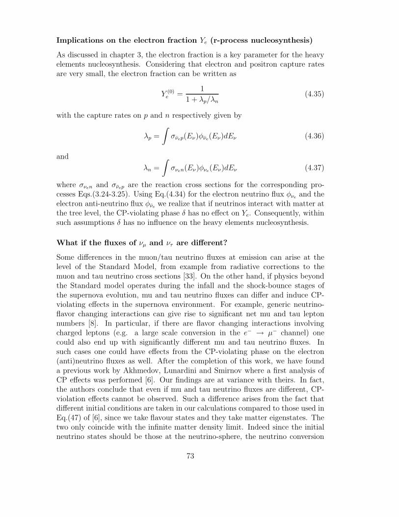
Implications on the electron fraction Ye (r-process nucleosynthesis)
As discussed in chapter 3, the electron fraction is a key parameter for the heavyelements nucleosynthesis. Considering that electron and positron capture ratesare very small, the electron fraction can be written as
Y (0)e =
1
1 + λp/λn
(4.35)
with the capture rates on p and n respectively given by
λp =
∫
σνep(Eν)φνe(Eν)dEν (4.36)
and
λn =
∫
σνen(Eν)φνe(Eν)dEν (4.37)
where σνen and σνep are the reaction cross sections for the corresponding pro-cesses Eqs.(3.24-3.25). Using Eq.(4.34) for the electron neutrino flux φνe
and theelectron anti-neutrino flux φνe
we realize that if neutrinos interact with matter atthe tree level, the CP-violating phase δ has no effect on Ye. Consequently, withinsuch assumptions δ has no influence on the heavy elements nucleosynthesis.
What if the fluxes of νµ and ντ are different?
Some differences in the muon/tau neutrino fluxes at emission can arise at thelevel of the Standard Model, from example from radiative corrections to themuon and tau neutrino cross sections [33]. On the other hand, if physics beyondthe Standard model operates during the infall and the shock-bounce stages ofthe supernova evolution, mu and tau neutrino fluxes can differ and induce CP-violating effects in the supernova environment. For example, generic neutrino-flavor changing interactions can give rise to significant net mu and tau leptonnumbers [8]. In particular, if there are flavor changing interactions involvingcharged leptons (e.g. a large scale conversion in the e− → µ− channel) onecould also end up with significantly different mu and tau neutrino fluxes. Insuch cases one could have effects from the CP-violating phase on the electron(anti)neutrino fluxes as well. After the completion of this work, we have founda previous work by Akhmedov, Lunardini and Smirnov where a first analysis ofCP effects was performed [6]. Our findings are at variance with theirs. In fact,the authors conclude that even if mu and tau neutrino fluxes are different, CP-violation effects cannot be observed. Such a difference arises from the fact thatdifferent initial conditions are taken in our calculations compared to those used inEq.(47) of [6], since we take flavour states and they take matter eigenstates. Thetwo only coincide with the infinite matter density limit. Indeed since the initialneutrino states should be those at the neutrino-sphere, the neutrino conversion
73
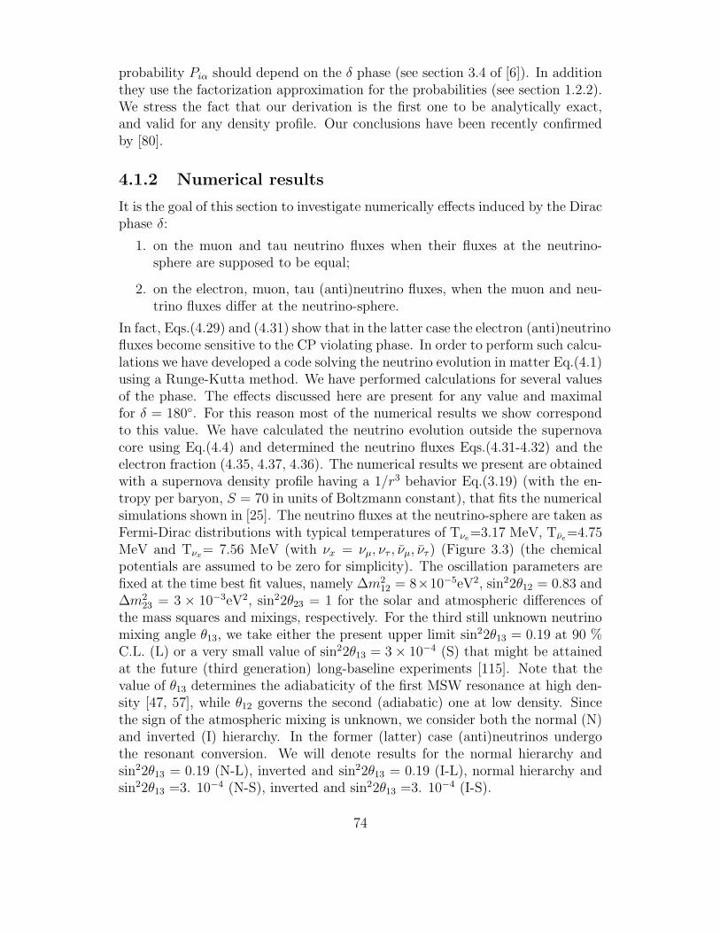
probability Piα should depend on the δ phase (see section 3.4 of [6]). In additionthey use the factorization approximation for the probabilities (see section 1.2.2).We stress the fact that our derivation is the first one to be analytically exact,and valid for any density profile. Our conclusions have been recently confirmedby [80].
4.1.2 Numerical results
It is the goal of this section to investigate numerically effects induced by the Diracphase δ:
1. on the muon and tau neutrino fluxes when their fluxes at the neutrino-sphere are supposed to be equal;
2. on the electron, muon, tau (anti)neutrino fluxes, when the muon and neu-trino fluxes differ at the neutrino-sphere.
In fact, Eqs.(4.29) and (4.31) show that in the latter case the electron (anti)neutrinofluxes become sensitive to the CP violating phase. In order to perform such calcu-lations we have developed a code solving the neutrino evolution in matter Eq.(4.1)using a Runge-Kutta method. We have performed calculations for several valuesof the phase. The effects discussed here are present for any value and maximalfor δ = 180. For this reason most of the numerical results we show correspondto this value. We have calculated the neutrino evolution outside the supernovacore using Eq.(4.4) and determined the neutrino fluxes Eqs.(4.31-4.32) and theelectron fraction (4.35, 4.37, 4.36). The numerical results we present are obtainedwith a supernova density profile having a 1/r3 behavior Eq.(3.19) (with the en-tropy per baryon, S = 70 in units of Boltzmann constant), that fits the numericalsimulations shown in [25]. The neutrino fluxes at the neutrino-sphere are taken asFermi-Dirac distributions with typical temperatures of Tνe
=3.17 MeV, Tνe=4.75
MeV and Tνx= 7.56 MeV (with νx = νµ, ντ , νµ, ντ ) (Figure 3.3) (the chemical
potentials are assumed to be zero for simplicity). The oscillation parameters arefixed at the time best fit values, namely ∆m2
12 = 8×10⁻⁵eV2, sin22θ12 = 0.83 and∆m2
23 = 3 × 10⁻³eV2, sin22θ23 = 1 for the solar and atmospheric differences ofthe mass squares and mixings, respectively. For the third still unknown neutrinomixing angle θ13, we take either the present upper limit sin22θ13 = 0.19 at 90 %C.L. (L) or a very small value of sin22θ13 = 3× 10⁻⁴ (S) that might be attainedat the future (third generation) long-baseline experiments [115]. Note that thevalue of θ13 determines the adiabaticity of the first MSW resonance at high den-sity [47, 57], while θ12 governs the second (adiabatic) one at low density. Sincethe sign of the atmospheric mixing is unknown, we consider both the normal (N)and inverted (I) hierarchy. In the former (latter) case (anti)neutrinos undergothe resonant conversion. We will denote results for the normal hierarchy andsin22θ13 = 0.19 (N-L), inverted and sin22θ13 = 0.19 (I-L), normal hierarchy andsin22θ13 =3. 10−4 (N-S), inverted and sin22θ13 =3. 10−4 (I-S).
74
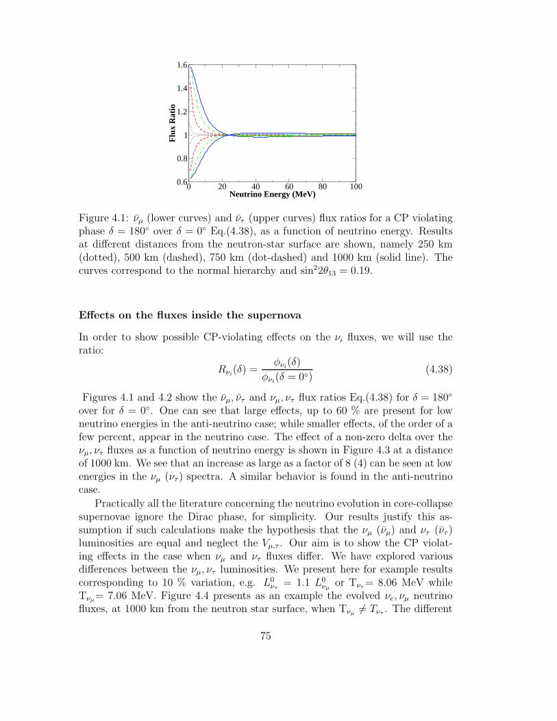
0 20 40 60 80 100Neutrino Energy (MeV)
0.6
0.8
1
1.2
1.4
1.6
Flu
x R
atio
Figure 4.1: νµ (lower curves) and ντ (upper curves) flux ratios for a CP violatingphase δ = 180 over δ = 0 Eq.(4.38), as a function of neutrino energy. Resultsat different distances from the neutron-star surface are shown, namely 250 km(dotted), 500 km (dashed), 750 km (dot-dashed) and 1000 km (solid line). Thecurves correspond to the normal hierarchy and sin22θ13 = 0.19.
Effects on the fluxes inside the supernova
In order to show possible CP-violating effects on the νi fluxes, we will use theratio:
Rνi(δ) =
φνi(δ)
φνi(δ = 0)
(4.38)
Figures 4.1 and 4.2 show the νµ, ντ and νµ, ντ flux ratios Eq.(4.38) for δ = 180
over for δ = 0. One can see that large effects, up to 60 % are present for lowneutrino energies in the anti-neutrino case; while smaller effects, of the order of afew percent, appear in the neutrino case. The effect of a non-zero delta over theνµ, ντ fluxes as a function of neutrino energy is shown in Figure 4.3 at a distanceof 1000 km. We see that an increase as large as a factor of 8 (4) can be seen at lowenergies in the νµ (ντ ) spectra. A similar behavior is found in the anti-neutrinocase.
Practically all the literature concerning the neutrino evolution in core-collapsesupernovae ignore the Dirac phase, for simplicity. Our results justify this as-sumption if such calculations make the hypothesis that the νµ (νµ) and ντ (ντ )luminosities are equal and neglect the Vµ,τ . Our aim is to show the CP violat-ing effects in the case when νµ and ντ fluxes differ. We have explored variousdifferences between the νµ, ντ luminosities. We present here for example resultscorresponding to 10 % variation, e.g. L0
ντ= 1.1 L0
νµor Tντ
= 8.06 MeV whileTνµ
= 7.06 MeV. Figure 4.4 presents as an example the evolved νe, νµ neutrinofluxes, at 1000 km from the neutron star surface, when Tνµ
6= Tντ. The different
75
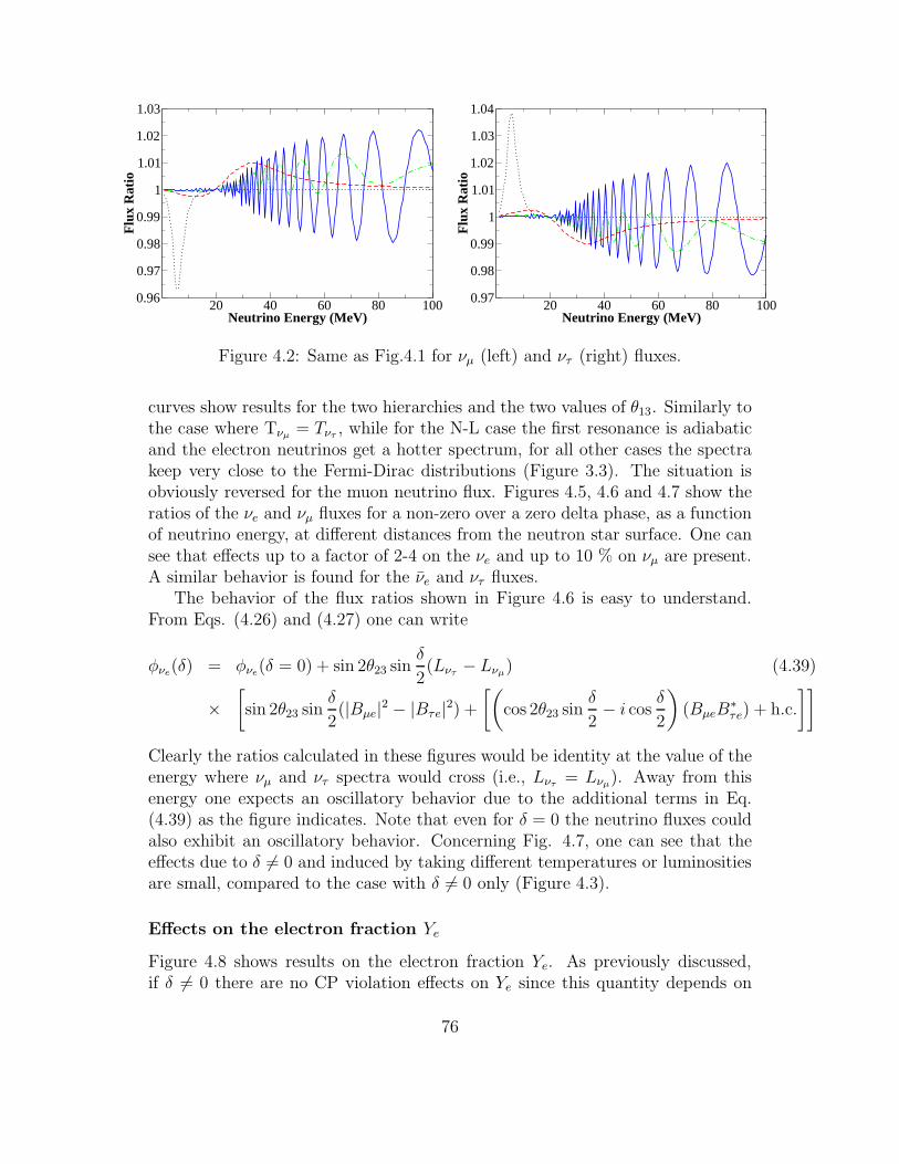
20 40 60 80 100Neutrino Energy (MeV)
0.96
0.97
0.98
0.99
1
1.01
1.02
1.03
Flu
x R
atio
20 40 60 80 100Neutrino Energy (MeV)
0.97
0.98
0.99
1
1.01
1.02
1.03
1.04
Flu
x R
atio
Figure 4.2: Same as Fig.4.1 for νµ (left) and ντ (right) fluxes.
curves show results for the two hierarchies and the two values of θ13. Similarly tothe case where Tνµ
= Tντ, while for the N-L case the first resonance is adiabatic
and the electron neutrinos get a hotter spectrum, for all other cases the spectrakeep very close to the Fermi-Dirac distributions (Figure 3.3). The situation isobviously reversed for the muon neutrino flux. Figures 4.5, 4.6 and 4.7 show theratios of the νe and νµ fluxes for a non-zero over a zero delta phase, as a functionof neutrino energy, at different distances from the neutron star surface. One cansee that effects up to a factor of 2-4 on the νe and up to 10 % on νµ are present.A similar behavior is found for the νe and ντ fluxes.
The behavior of the flux ratios shown in Figure 4.6 is easy to understand.From Eqs. (4.26) and (4.27) one can write
φνe(δ) = φνe
(δ = 0) + sin 2θ23 sinδ
2(Lντ
− Lνµ) (4.39)
×[
sin 2θ23 sinδ
2(|Bµe|2 − |Bτe|2) +
[(
cos 2θ23 sinδ
2− i cos
δ
2
)
(BµeB∗τe) + h.c.
]]
Clearly the ratios calculated in these figures would be identity at the value of theenergy where νµ and ντ spectra would cross (i.e., Lντ
= Lνµ). Away from this
energy one expects an oscillatory behavior due to the additional terms in Eq.(4.39) as the figure indicates. Note that even for δ = 0 the neutrino fluxes couldalso exhibit an oscillatory behavior. Concerning Fig. 4.7, one can see that theeffects due to δ 6= 0 and induced by taking different temperatures or luminositiesare small, compared to the case with δ 6= 0 only (Figure 4.3).
Effects on the electron fraction Ye
Figure 4.8 shows results on the electron fraction Ye. As previously discussed,if δ 6= 0 there are no CP violation effects on Ye since this quantity depends on
76
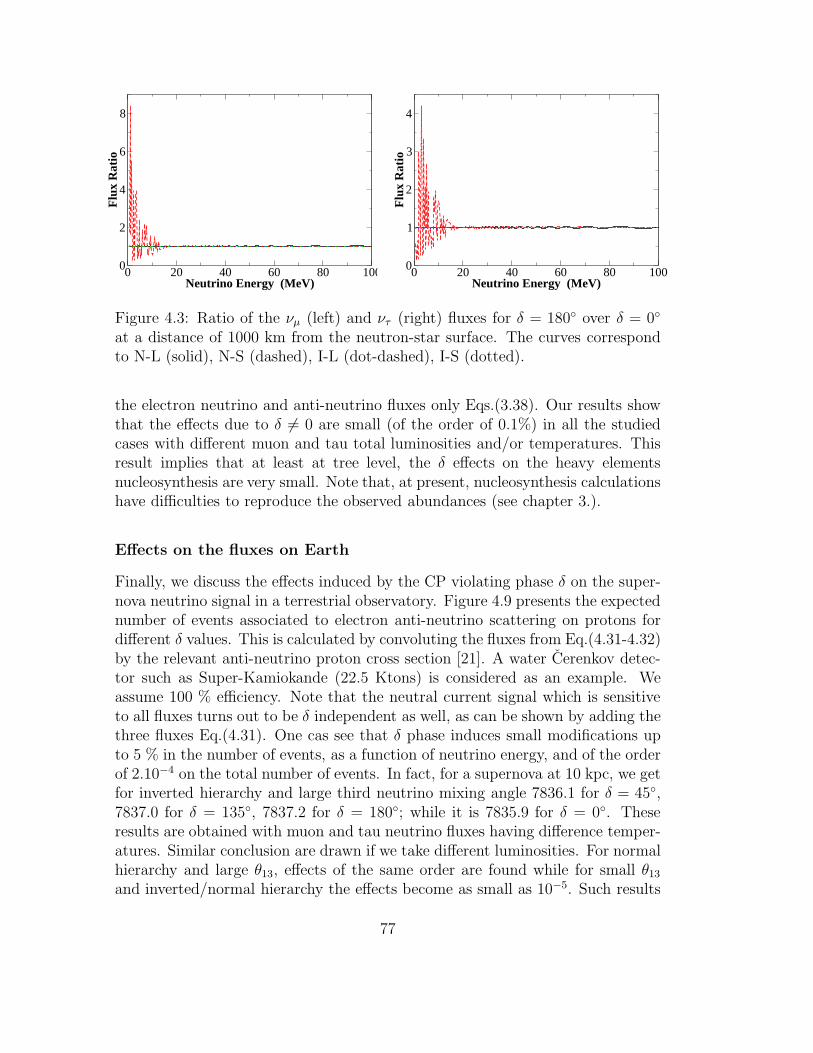
0 20 40 60 80 100Neutrino Energy (MeV)
0
2
4
6
8F
lux
Rat
io
0 20 40 60 80 100Neutrino Energy (MeV)
0
1
2
3
4
Flu
x R
atio
Figure 4.3: Ratio of the νµ (left) and ντ (right) fluxes for δ = 180 over δ = 0
at a distance of 1000 km from the neutron-star surface. The curves correspondto N-L (solid), N-S (dashed), I-L (dot-dashed), I-S (dotted).
the electron neutrino and anti-neutrino fluxes only Eqs.(3.38). Our results showthat the effects due to δ 6= 0 are small (of the order of 0.1%) in all the studiedcases with different muon and tau total luminosities and/or temperatures. Thisresult implies that at least at tree level, the δ effects on the heavy elementsnucleosynthesis are very small. Note that, at present, nucleosynthesis calculationshave difficulties to reproduce the observed abundances (see chapter 3.).
Effects on the fluxes on Earth
Finally, we discuss the effects induced by the CP violating phase δ on the super-nova neutrino signal in a terrestrial observatory. Figure 4.9 presents the expectednumber of events associated to electron anti-neutrino scattering on protons fordifferent δ values. This is calculated by convoluting the fluxes from Eq.(4.31-4.32)by the relevant anti-neutrino proton cross section [21]. A water Cerenkov detec-tor such as Super-Kamiokande (22.5 Ktons) is considered as an example. Weassume 100 % efficiency. Note that the neutral current signal which is sensitiveto all fluxes turns out to be δ independent as well, as can be shown by adding thethree fluxes Eq.(4.31). One cas see that δ phase induces small modifications upto 5 % in the number of events, as a function of neutrino energy, and of the orderof 2.10−4 on the total number of events. In fact, for a supernova at 10 kpc, we getfor inverted hierarchy and large third neutrino mixing angle 7836.1 for δ = 45,7837.0 for δ = 135, 7837.2 for δ = 180; while it is 7835.9 for δ = 0. Theseresults are obtained with muon and tau neutrino fluxes having difference temper-atures. Similar conclusion are drawn if we take different luminosities. For normalhierarchy and large θ13, effects of the same order are found while for small θ13and inverted/normal hierarchy the effects become as small as 10−5. Such results
77
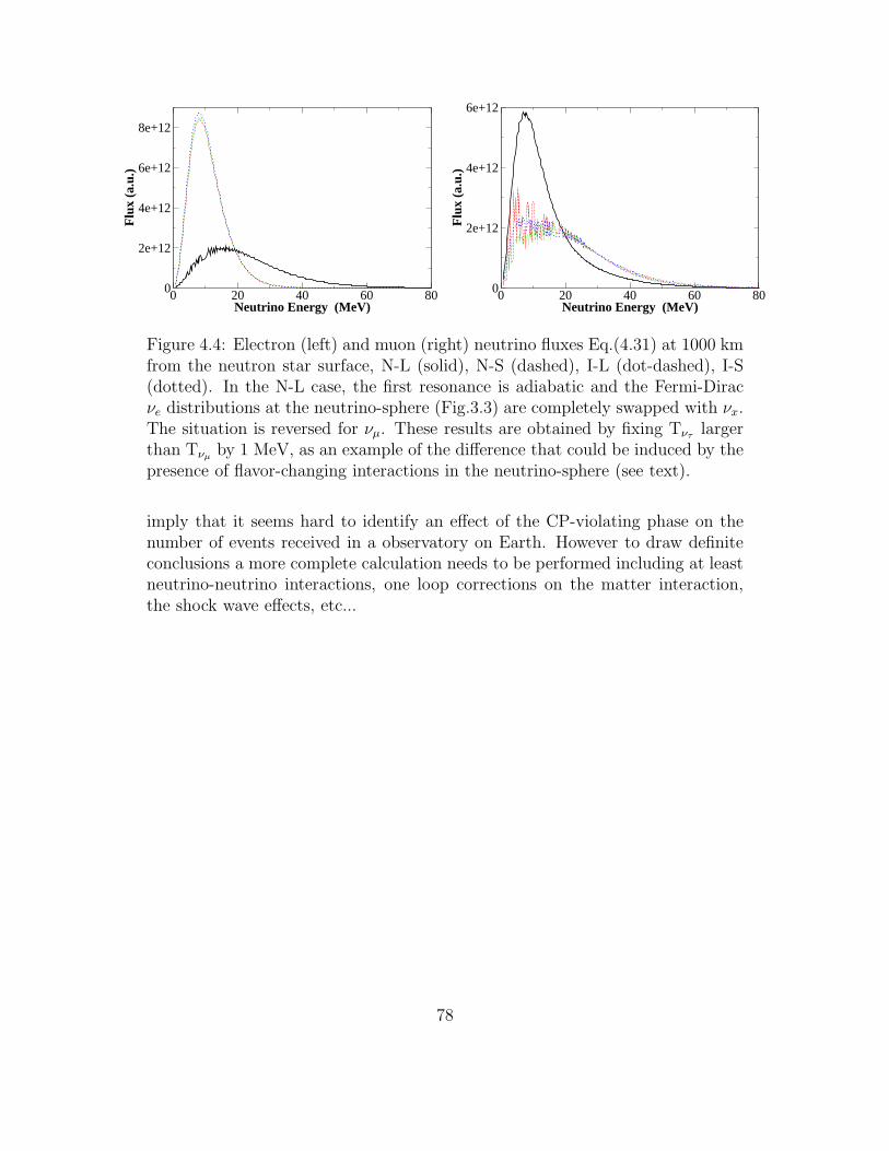
0 20 40 60 80Neutrino Energy (MeV)
0
2e+12
4e+12
6e+12
8e+12F
lux
(a.u
.)
0 20 40 60 80Neutrino Energy (MeV)
0
2e+12
4e+12
6e+12
Flu
x (a
.u.)
Figure 4.4: Electron (left) and muon (right) neutrino fluxes Eq.(4.31) at 1000 kmfrom the neutron star surface, N-L (solid), N-S (dashed), I-L (dot-dashed), I-S(dotted). In the N-L case, the first resonance is adiabatic and the Fermi-Diracνe distributions at the neutrino-sphere (Fig.3.3) are completely swapped with νx.The situation is reversed for νµ. These results are obtained by fixing Tντ
largerthan Tνµ
by 1 MeV, as an example of the difference that could be induced by thepresence of flavor-changing interactions in the neutrino-sphere (see text).
imply that it seems hard to identify an effect of the CP-violating phase on thenumber of events received in a observatory on Earth. However to draw definiteconclusions a more complete calculation needs to be performed including at leastneutrino-neutrino interactions, one loop corrections on the matter interaction,the shock wave effects, etc...
78
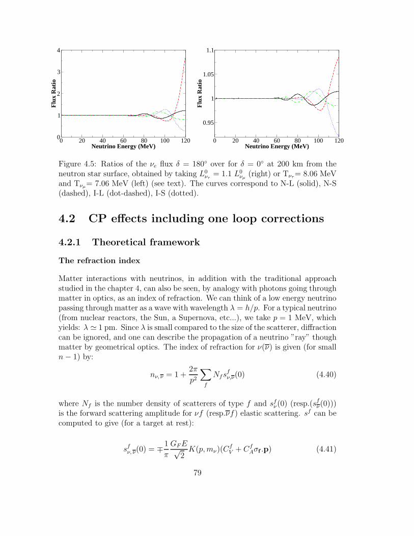
0 20 40 60 80 100 120Neutrino Energy (MeV)
0
1
2
3
4F
lux
Rat
io
0 20 40 60 80 100 120Neutrino Energy (MeV)
0.95
1
1.05
1.1
Flu
x R
atio
Figure 4.5: Ratios of the νe flux δ = 180 over for δ = 0 at 200 km from theneutron star surface, obtained by taking L0
ντ= 1.1 L0
νµ(right) or Tντ
= 8.06 MeVand Tνµ
= 7.06 MeV (left) (see text). The curves correspond to N-L (solid), N-S(dashed), I-L (dot-dashed), I-S (dotted).
4.2 CP effects including one loop corrections
4.2.1 Theoretical framework
The refraction index
Matter interactions with neutrinos, in addition with the traditional approachstudied in the chapter 4, can also be seen, by analogy with photons going throughmatter in optics, as an index of refraction. We can think of a low energy neutrinopassing through matter as a wave with wavelength λ = h/p. For a typical neutrino(from nuclear reactors, the Sun, a Supernova, etc...), we take p = 1 MeV, whichyields: λ ≃ 1 pm. Since λ is small compared to the size of the scatterer, diffractioncan be ignored, and one can describe the propagation of a neutrino ”ray” thoughmatter by geometrical optics. The index of refraction for ν(ν) is given (for smalln− 1) by:
nν, ν = 1 +2π
p2
∑
f
Nfsfν,ν(0) (4.40)
where Nf is the number density of scatterers of type f and sfν(0) (resp.(sf
ν(0)))is the forward scattering amplitude for νf (resp.νf) elastic scattering. sf can becomputed to give (for a target at rest):
sfν, ν(0) = ∓1
π
GFE√2K(p,mν)(C
fV + Cf
Aσf .p) (4.41)
79
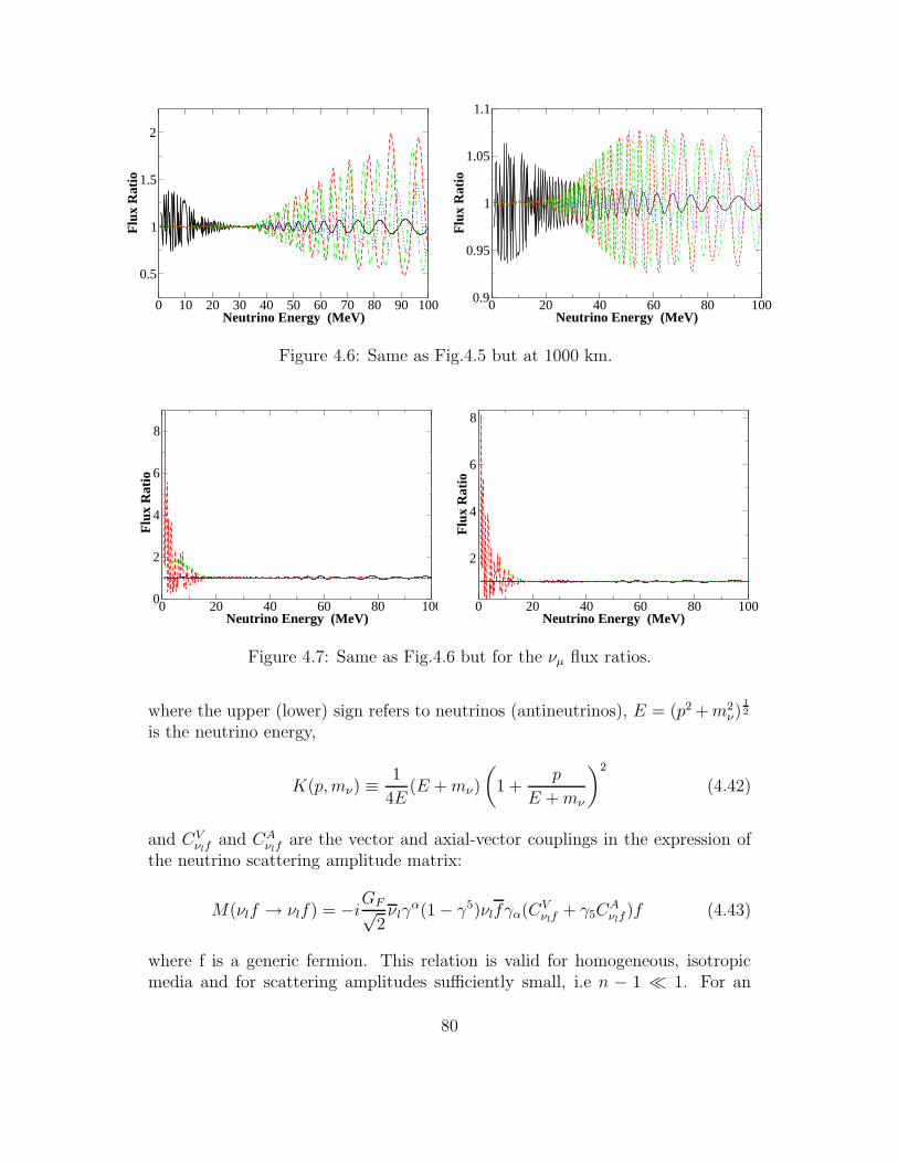
0 10 20 30 40 50 60 70 80 90 100Neutrino Energy (MeV)
0.5
1
1.5
2F
lux
Rat
io
0 20 40 60 80 100Neutrino Energy (MeV)
0.9
0.95
1
1.05
1.1
Flu
x R
atio
Figure 4.6: Same as Fig.4.5 but at 1000 km.
0 20 40 60 80 100Neutrino Energy (MeV)
0
2
4
6
8
Flu
x R
atio
0 20 40 60 80 100Neutrino Energy (MeV)
2
4
6
8
Flu
x R
atio
Figure 4.7: Same as Fig.4.6 but for the νµ flux ratios.
where the upper (lower) sign refers to neutrinos (antineutrinos), E = (p2 +m2ν)
12
is the neutrino energy,
K(p,mν) ≡1
4E(E +mν)
(
1 +p
E +mν
)2
(4.42)
and CVνlf
and CAνlf
are the vector and axial-vector couplings in the expression ofthe neutrino scattering amplitude matrix:
M(νlf → νlf) = −iGF√2νlγ
α(1− γ5)νlfγα(CVνlf
+ γ5CAνlf
)f (4.43)
where f is a generic fermion. This relation is valid for homogeneous, isotropicmedia and for scattering amplitudes sufficiently small, i.e n − 1 ≪ 1. For an
80
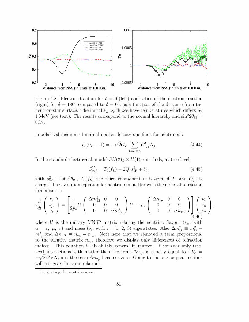
2 4 6 8 10distance from NSS (in units of 100 Km)
0.3
0.4
0.5
0.6
0.7Y
e
theta13=9° NHtheta13=0.5° NHtheta13=9° IHtheta13=0.5° IH
2 4 6 8 10distance from NSS (in units of 100 Km)
0.9995
1
1.0005
1,001
Ye
Figure 4.8: Electron fraction for δ = 0 (left) and ratios of the electron fraction(right) for δ = 180 compared to δ = 0, as a function of the distance from theneutron-star surface. The initial νµ, ντ fluxes have temperatures which differs by1 MeV (see text). The results correspond to the normal hierarchy and sin22θ13 =0.19.
unpolarized medium of normal matter density one finds for neutrinos3:
pν(nνl− 1) = −
√2GF
∑
f=e,u,d
CVνlfNf (4.44)
In the standard electroweak model SU(2)L × U(1), one finds, at tree level,
CVνℓf
= T3(fL)− 2Qfs2W + δℓf (4.45)
with s2W ≡ sin2 θW , T3(fL) the third component of isospin of fL and Qf its
charge. The evolution equation for neutrino in matter with the index of refractionformalism is:
id
dt
νe
νµ
ντ
=
1
2pνU
∆m212 0 0
0 0 00 0 ∆m2
32
U † − pν
∆neµ 0 00 0 00 0 ∆nτµ
νe
νµ
ντ
,
(4.46)where U is the unitary MNSP matrix relating the neutrino flavour (να, withα = e, µ, τ) and mass (νi, with i = 1, 2, 3) eigenstates. Also ∆m2
ij ≡ m2νi−
m2νj
and ∆nαβ ≡ nνα− nνβ
. Note here that we removed a term proportionalto the identity matrix nνµ
, therefore we display only differences of refractionindices. This equation is absolutely general in matter. If consider only tree-level interactions with matter then the term ∆neµ is strictly equal to −Ve =−√
2GF Ne and the term ∆nτµ becomes zero. Going to the one-loop correctionswill not give the same relations.
3neglecting the neutrino mass.
81
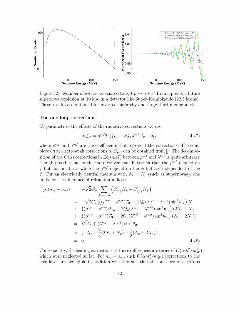
50 100 150Neutrino Energy (MeV)
0.01
1
100N
umbe
r of
Eve
nts
50 100 150Neutrino Energy (MeV)
0.96
0.98
1
1.02
1.04
Num
ber
of E
vent
s R
atio
NEvents( δ =135°)/NEvents(δ = 0°)NEvents(δ =180°)/NEvents(δ =0°)NEvents ( δ =45°)/NEvents( δ =0°)
Figure 4.9: Number of events associated to νe +p→ n+e+ from a possible futuresupernova explosion at 10 kpc in a detector like Super-Kamiokande (22.5 ktons).These results are obtained for inverted hierarchy and large third mixing angle.
The one-loop corrections
To parametrise the effects of the radiative corrections we use:
CVνℓf
= ρνℓfT3(fL)− 2Qfλνℓfs2
W + δℓf (4.47)
where ρνℓf and λνℓf are the coefficients that represent the corrections. The com-plete O(α) electroweak corrections to CV
νℓfcan be obtained from []. The decompo-
sition of the O(α) corrections in Eq.(4.47) between ρνℓf and λνℓf is quite arbitrarythough possible and furthermore convenient. It is such that the ρνℓf depend onf but not on the νl while the λνℓf depend on the νl but are independent of thef . For an electrically neutral medium with Ne = Np (such as supernovae), onefinds for the difference of refraction indices:
pν(nνℓ− nνℓ′
) = −√
2GF
∑
f=e,u,d
(
CVνℓfNf − CV
νℓ′fNf
)
= −√
2GF [(
(ρνℓe − ρνℓ′e)T3e − 2Qe(λνℓe − λνℓ′e) sin2 θW
)
Ne
+(
(ρνℓu − ρνℓ′u)T3u − 2Qu(λνℓu − λνℓ′u) sin2 θW
)
(2Ne +Nn)
+(
(ρνℓd − ρνℓ′d)T3u − 2Qd(λνℓd − λνℓ′d) sin2 θW
)
(Ne + 2Nn)]
=√
2GF [2(λνℓf − λνℓ′f ) sin2 θW
× (−Ne +2
3(2Ne +Nn)− 1
3(Ne + 2Nn)]
= 0 (4.48)
Consequently, the leading corrections to those differences are terms ofO(αm2τ/m
2W )
which were neglected so far. For nνe− nνµ
, such O(αm2µ/m
2W ) corrections to the
tree level are negligible in addition with the fact that the presence of electrons
82
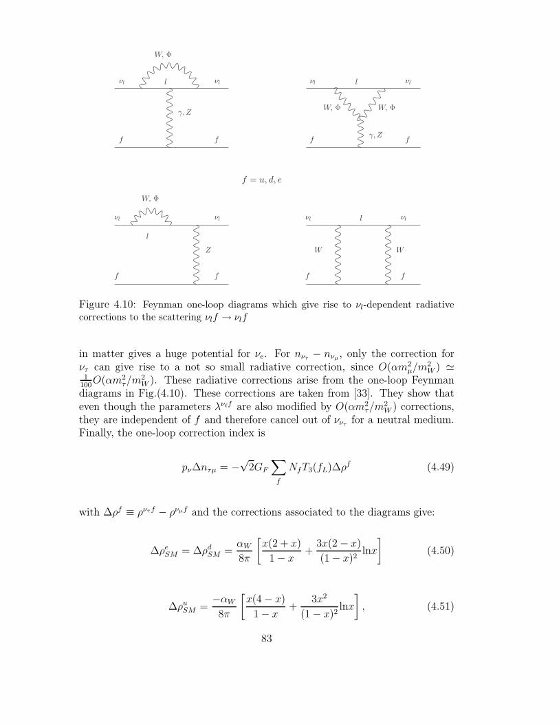
νl νl
νl
νl νl
νl νlνl
W, Φ
f = u, d, e
W, Φ
W, Φ W, Φγ, Z
γ, Z
Z W W
l
l
l
l
f f
f f f f
f f
Figure 4.10: Feynman one-loop diagrams which give rise to νl-dependent radiativecorrections to the scattering νlf → νlf
in matter gives a huge potential for νe. For nντ− nνµ
, only the correction forντ can give rise to a not so small radiative correction, since O(αm2
µ/m2W ) ≃
1100O(αm2
τ/m2W ). These radiative corrections arise from the one-loop Feynman
diagrams in Fig.(4.10). These corrections are taken from [33]. They show thateven though the parameters λνℓf are also modified by O(αm2
τ/m2W ) corrections,
they are independent of f and therefore cancel out of νντfor a neutral medium.
Finally, the one-loop correction index is
pν∆nτµ = −√
2GF
∑
f
NfT3(fL)∆ρf (4.49)
with ∆ρf ≡ ρντ f − ρνµf and the corrections associated to the diagrams give:
∆ρeSM = ∆ρd
SM =αW
8π
[
x(2 + x)
1− x +3x(2− x)(1− x)2
lnx
]
(4.50)
∆ρuSM =
−αW
8π
[
x(4− x)1− x +
3x2
(1− x)2lnx
]
, (4.51)
83
with x ≡ m2τ/M
2W and αW ≡ α/s2
W . For a neutral unpolarized medium withNe = Np and arbitrary Nn one finds from Eq.(4.50) and Eq.(4.51):
pν(nντ− nνµ
) =GF√
2
3α
2π sin2 θW
m2τ
m2W
×[
(Nn +Np) ln
(
m2τ
m2W
)
+Np +2
3
]
(4.52)
Factorizing out (Nn +Np) and using the equality
GF =απ√
2 sin2 θWm2W
(4.53)
one obtains:
pν(nντ− nνµ
) =3G2
Fm2τ
2π2
[
ln
(
m2τ
m2W
)
+Np
Nn +Np+
2
3
Nn
Nn +Np
]
(Nn +Np)
= −√
2GF3√
2GFm2τ
(2π)2Ye
[
ln
(
m2W
m2τ
)
+Yn
3− 1
]
Ne
= −√
2GFY eff
τ
YeNe
= −√
2GFYeffτ NB (4.54)
where NB is the baryon density in the medium. Thus, we can see these radiativecorrections as an effective matter of τ depending on the electron density Ne. Foran isoscalar medium with Nn = Np = Ne, we have:
pν(nντ− nνµ
) = −√
2GF6√
2GFm2τ
(2π)2
[
ln
(
m2W
m2τ
)
− 5
6
]
Ne (4.55)
andY eff
τ ≃ 5.4× 10⁻⁵ (4.56)
Finally, the potential due to these one-loop radiative corrections is
Vµτ =√
2GFY eff
τ
YeNe. (4.57)
Vµτ =√
2GF3√
2GFm2τ
(2π)2Ye
[
ln
(
m2W
m2τ
)
+Yn
3− 1
]
Ne (4.58)
Though this term seems very small, it is not negligible and can lead to effectsinside the supernova like a resonance between νµ and ντ neutrinos [61]. Contraryto what was commonly thought, it can even leads to theoretically observableeffects on the νe and νe fluxes inside the supernova, affecting consequently Ye andeven on Earth, all of those via the presence of the CP-violating phase.
84
4.2.2 Explicit CP-violation phase dependence
The factorization?
If we include the radiative corrections to the interactions with matter, the neu-trino evolution equations get modified:
i∂
∂t
Ψe
Ψµ
Ψτ
=
T23T13T12
E1 0 00 E2 00 0 E3
T †12T
†13T
†23 +
Vc 0 00 0 00 0 Vµτ
Ψe
Ψµ
Ψτ
.
(4.59)As seen in the case of interactions with matter at tree level, to obtain explicitrelations between probabilities and the CP-violating phase, it is necessary to workwithin a new basis where a rotation by T23 is performed. In this case, factorizingthe S matrix containing δ, out of the Hamiltonian, one has:
i∂
∂t
Ψe
Ψµ
Ψτ
= HT (δ)
Ψe
Ψµ
Ψτ
= S H ′T (δ)S†
Ψe
Ψµ
Ψτ
= S
T 013T12
E1 0 00 E2 00 0 E3
T †12T
013
†(4.60)
+
Vc 0 00 s2
23 Vµτ −c23s23eiδ Vµτ
0 −c23s23e−iδ Vµτ c223 Vµτ
S†
Ψe
Ψµ
Ψτ
,
Contrary to Eq.(4.9), the S matrix does not commute with the matter Hamilto-nian in the T23 basis. This fact implies that:
HT (δ) 6= S HT (δ = 0)S†, (4.61)
and therefore that
Um(δ) 6= SUm(δ = 0)S†. (4.62)
Consequence on the electron neutrino survival probability
Nevertheless, we can factorize the S matrices but we will have an Hamiltonianwhich depends on δ. We can rewrite Eq.(4.60) in the evolution operator formalismto have:
i∂
∂t
Aee Aµe Aτ eeiδ
Aeµ Aµµ Aτ µeiδ
Aeτe−iδ Aµτe
−iδ Aτ τ
= H ′T (δ)
Aee Aµe Aτ eeiδ
Aeµ Aµµ Aτ µeiδ
Aeτe−iδ Aµτe
−iδ Aτ τ
(4.63)
85
Defining the Hamiltonian H ′T (δ) by4:
H ′T (δ) =
a b cb d (e− g eiδ)c (e− g e−iδ) f
(4.64)
we can write the evolution equations for the amplitudes process of the first col-umn of the evolution operator, which corresponds to the creation of an electronneutrino νe initially:
id
dtAee = aAee + bAeµ + cAeτe
−iδ
id
dtAeµ = bAee + dAeµ + (e− g eiδ)Aeτe
−iδ
id
dtAeτe
−iδ = cAee + (e− g eiδ)Aeµ + f Aeτe−iδ (4.65)
Similarly, we can write the same equation for the amplitudes Bαβ when δ is takento be zero and look at the difference between the amplitudes that depend on δand those which don’t. The basic idea here is to prove that, because of the one-loop correction term Vµτ , the function Aee−Bee is not the constant zero functionby showing that its derivative is non zero.
id
dt(Aee − Bee) = a (Aee − Bee) + b (Aeµ − Beµ) + c (Aeτe
−iδ − Beτ ) (4.66)
id
dt(Aeµ −Beµ) = b (Aee −Bee) + d (Aeµ −Beµ) + e (Aeτe
−iδ − Beτ) + g (Aeτ −Beτ )
id
dt(Aeτe
−iδ − Beτ ) = c (Aee − Bee) + e (Aeµ −Aeµ) + f (Aeτe−iδ − Beτ )− g (Aeµe
−iδ − Beµ)
Let us now take a closer look at Eqs.(4.66). The initial condition we are interestedin, namely a νe created initially means that initially the amplitudes A and B are:
Ψe
Ψµ
Ψτ
=
100
⇒
Aee
Aeµ
Aeτe−iδ
=
Bee
Beµ
Beτ
=
100
(4.67)
When g = 0 (Vµτ = 0), it is easy to see that injecting the initial conditions inEqs.(4.66) will imply that the functions fe = Aee − Bee, fµ = Aeµ − Beµ andfτ = Aeτe
−iδ − Beτ will be equal to the zero function. Indeed, discretizing timewe see by recurrence that if those functions are zero at beginning, the will beequal to zero at all time. But when g 6= 0 (Vµτ 6= 0) we have to look also at
the evolution of the functions fµ = Aeµe−iδ − Beµ and fτ = Aeτ − Beτ . Their
4a, b, c, d, e ,f and g are real.
86
respective evolution equation can be easily derived from Eq.(4.65) to yield:
id
dt(Aeµe
−iδ−Beµ) = b (Aeee−iδ−Bee)+d (Aeµe
−iδ−Beµ)+e (Aeτe−2iδ−Beτ )+g (Aeτe
−iδ−Beτ )
(4.68)
id
dt(Aeτ−Beτ ) = c (Aeee
iδ−Bee)+e (Aeµeiδ−Aeµ)+f (Aeτ−Beτ )−g (Aeµ−Beµ)
(4.69)Initially, the derivatives are :
id
dt(Aeµe
−iδ −Beµ)(t = 0) = id
dtf ′
µ(t = 0) = b(e−iδ − 1)
id
dt(Aeτ − Beτ )(t = 0) = i
d
dtf ′
τ (t = 0) = c(eiδ − 1) (4.70)
We just proved that since the functions fµ and fτ are non constant zero functions,the functions fµ and fτ won’t be zero as well. But does it implies that the function
fe is non zero at all time? No, because the contributions from fµ and fτ couldcancel in the evolution equation (4.66) of fe. To precisely study the evolution offe, we discretize time such as t = N ∗∆t with N ∈ N and
d
dtfe =
fe(t+ ∆t)− fe(t)
∆t(4.71)
Using Eqs.(4.66) and the time discretization we see that: At t = ∆t:
f ′µ(∆t) =
b(e−iδ − 1)
i∆t
f ′τ (∆t) =
c(eiδ − 1)
i∆t
(4.72)
which implies that: At t = 2∆t:
fµ(2∆t) = gb(e−iδ − 1)∆2t
fτ (2∆t) = −gc(eiδ − 1)∆2t
(4.73)
leading at t = 3∆t
fe(3∆t) =1
i
(
gbc(e−iδ − 1)− gbc(eiδ − 1))
∆3t
=1
igbc(e−iδ − eiδ)∆3t
= −2gbc sin δ∆3t (4.74)
87
This last formula prove that the function fe is not the constant zero functionAee 6= Bee and consequently:
P (νe → νe, δ 6= 0) 6= P (νe → νe, δ = 0) (4.75)
Therefore , when δ is taken non zero, it has an influence on the value of P (νe →νe, δ). The νe and νe fluxes will depend on δ even when the luminosities Lνµ
andLντ
are taken equal at the neutrino-sphere:
φνe(δ) = Lνe
P (νe → νe, δ) + Lνµ(P (νµ → νe) + P (ντ → νe))
= LνeP (νe → νe, δ) + Lνµ
(1− P (νe → νe, δ))
= (Lνe− Lνµ
)P (νe → νe, δ) + Lνµ(4.76)
This analytical derivation proving that, if the dependence on δ of the evolutionoperator cannot be factorized then the electron neutrino survival probability de-pends on δ, is the first to be performed. Nevertheless, this implication had beenobserved numerically. We can easily generalize this derivation which implies thatas soon as the medium effect on νµ and on ντ is not the same, effects of the CP-violating phase on the electron neutrino (and anti-neutrino) fluxes will appear.
88
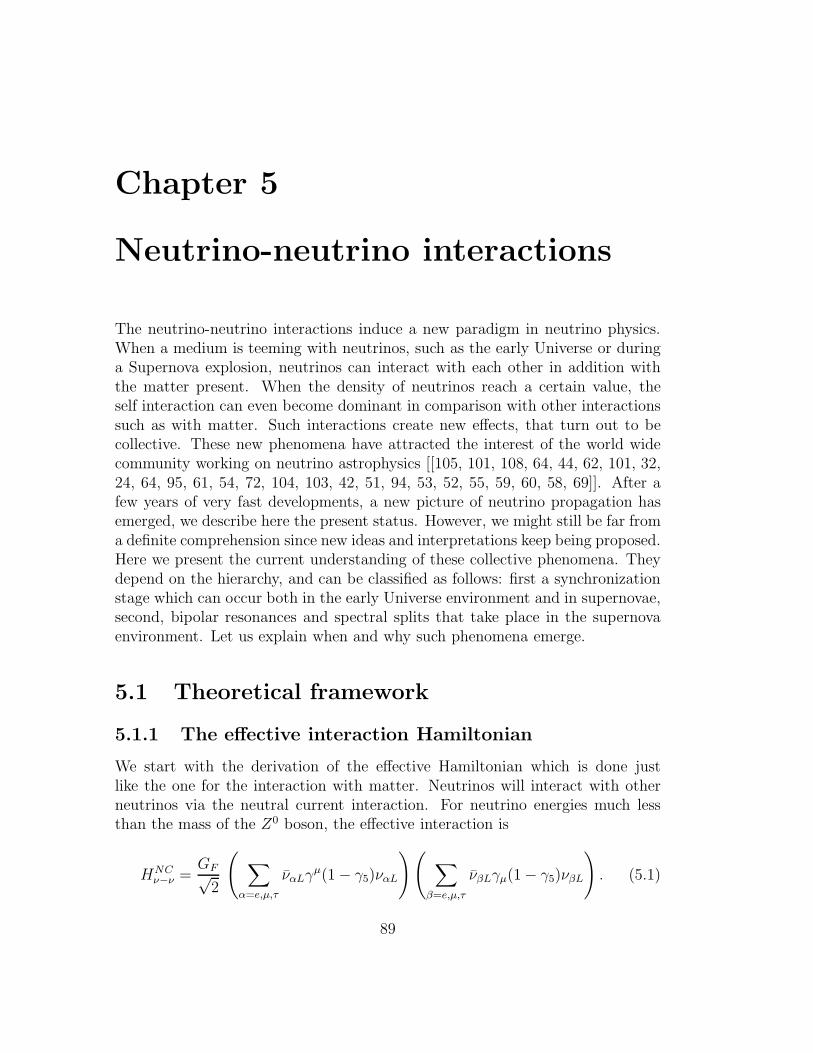
Chapter 5
Neutrino-neutrino interactions
The neutrino-neutrino interactions induce a new paradigm in neutrino physics.When a medium is teeming with neutrinos, such as the early Universe or duringa Supernova explosion, neutrinos can interact with each other in addition withthe matter present. When the density of neutrinos reach a certain value, theself interaction can even become dominant in comparison with other interactionssuch as with matter. Such interactions create new effects, that turn out to becollective. These new phenomena have attracted the interest of the world widecommunity working on neutrino astrophysics [[105, 101, 108, 64, 44, 62, 101, 32,24, 64, 95, 61, 54, 72, 104, 103, 42, 51, 94, 53, 52, 55, 59, 60, 58, 69]]. After afew years of very fast developments, a new picture of neutrino propagation hasemerged, we describe here the present status. However, we might still be far froma definite comprehension since new ideas and interpretations keep being proposed.Here we present the current understanding of these collective phenomena. Theydepend on the hierarchy, and can be classified as follows: first a synchronizationstage which can occur both in the early Universe environment and in supernovae,second, bipolar resonances and spectral splits that take place in the supernovaenvironment. Let us explain when and why such phenomena emerge.
5.1 Theoretical framework
5.1.1 The effective interaction Hamiltonian
We start with the derivation of the effective Hamiltonian which is done justlike the one for the interaction with matter. Neutrinos will interact with otherneutrinos via the neutral current interaction. For neutrino energies much lessthan the mass of the Z0 boson, the effective interaction is
HNCν−ν =
GF√2
(
∑
α=e,µ,τ
ναLγµ(1− γ5)ναL
)(
∑
β=e,µ,τ
νβLγµ(1− γ5)νβL
)
. (5.1)
89
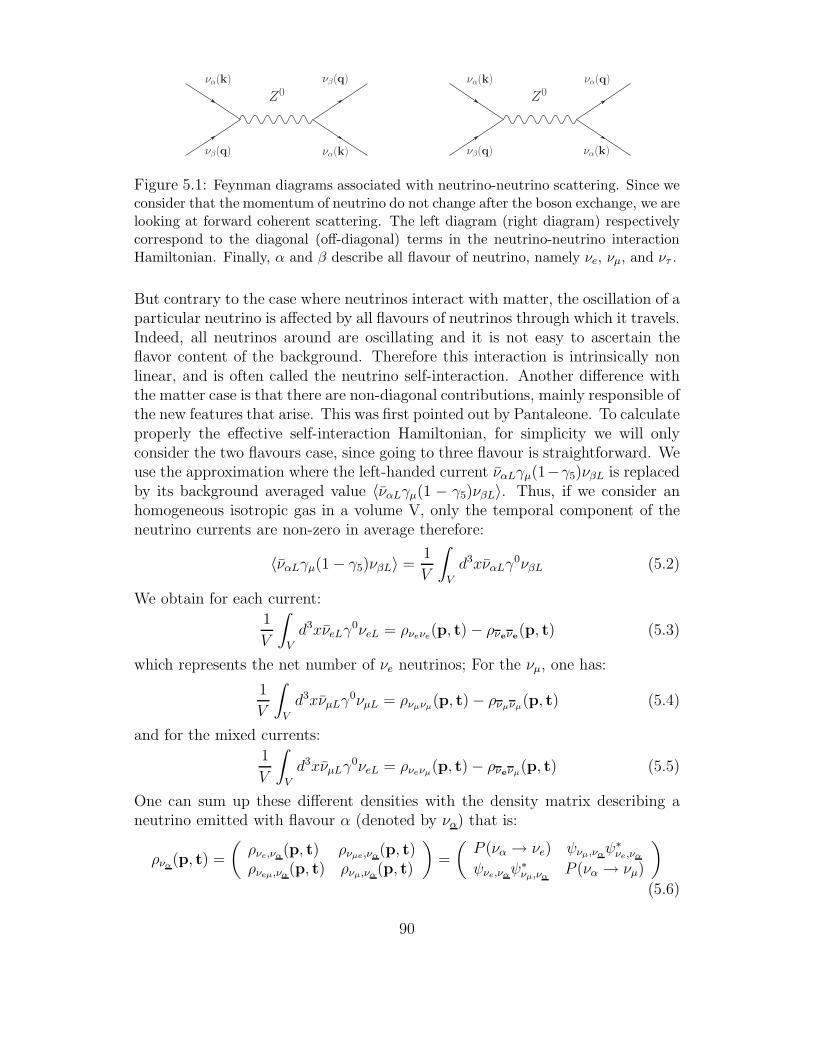
Z0 Z0να(k) να(k) να(q)νβ(q)
νβ(q) να(k) νβ(q) να(k)
Figure 5.1: Feynman diagrams associated with neutrino-neutrino scattering. Since weconsider that the momentum of neutrino do not change after the boson exchange, we arelooking at forward coherent scattering. The left diagram (right diagram) respectivelycorrespond to the diagonal (off-diagonal) terms in the neutrino-neutrino interactionHamiltonian. Finally, α and β describe all flavour of neutrino, namely νe, νµ, and ντ .
But contrary to the case where neutrinos interact with matter, the oscillation of aparticular neutrino is affected by all flavours of neutrinos through which it travels.Indeed, all neutrinos around are oscillating and it is not easy to ascertain theflavor content of the background. Therefore this interaction is intrinsically nonlinear, and is often called the neutrino self-interaction. Another difference withthe matter case is that there are non-diagonal contributions, mainly responsible ofthe new features that arise. This was first pointed out by Pantaleone. To calculateproperly the effective self-interaction Hamiltonian, for simplicity we will onlyconsider the two flavours case, since going to three flavour is straightforward. Weuse the approximation where the left-handed current ναLγµ(1−γ5)νβL is replacedby its background averaged value 〈ναLγµ(1 − γ5)νβL〉. Thus, if we consider anhomogeneous isotropic gas in a volume V, only the temporal component of theneutrino currents are non-zero in average therefore:
〈ναLγµ(1− γ5)νβL〉 =1
V
∫
V
d3xναLγ0νβL (5.2)
We obtain for each current:
1
V
∫
V
d3xνeLγ0νeL = ρνeνe
(p, t)− ρνeνe(p, t) (5.3)
which represents the net number of νe neutrinos; For the νµ, one has:
1
V
∫
V
d3xνµLγ0νµL = ρνµνµ
(p, t)− ρνµνµ(p, t) (5.4)
and for the mixed currents:
1
V
∫
V
d3xνµLγ0νeL = ρνeνµ
(p, t)− ρνeνµ(p, t) (5.5)
One can sum up these different densities with the density matrix describing aneutrino emitted with flavour α (denoted by να) that is:
ρνα(p, t) =
(
ρνe,να(p, t) ρνµe,να
(p, t)ρνeµ,να
(p, t) ρνµ,να(p, t)
)
=
(
P (να → νe) ψνµ,ναψ∗
νe,να
ψνe,ναψ∗
νµ,ναP (να → νµ)
)
(5.6)
90
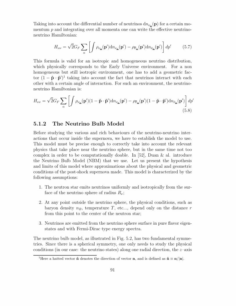
Taking into account the differential number of neutrinos dnνα(p) for a certain mo-
mentum p and integrating over all momenta one can write the effective neutrino-neutrino Hamiltonian:
Hνν =√
2GF
∑
α
[∫
ρνα(p′)dnνα
(p′)− ρνα(p′)dnνα
(p′)
]
dp′ (5.7)
This formula is valid for an isotropic and homogeneous neutrino distribution,which physically corresponds to the Early Universe environment. For a nonhomogeneous but still isotropic environment, one has to add a geometric fac-tor (1 − p · p′)1 taking into account the fact that neutrinos interact with eachother with a certain angle of interaction. For such an environment, the neutrino-neutrino Hamiltonian is:
Hνν =√
2GF
∑
α
[∫
ρνα(p′)(1− p · p′)dnνα
(p′)− ρνα(p′)(1− p · p′)dnνα
(p′)
]
dp′
(5.8)
5.1.2 The Neutrino Bulb Model
Before studying the various and rich behaviours of the neutrino-neutrino inter-actions that occur inside the supernova, we have to establish the model to use.This model must be precise enough to correctly take into account the relevantphysics that take place near the neutrino sphere, but in the same time not toocomplex in order to be computationally doable. In [52], Duan & al. introducethe Neutrino Bulb Model (NBM) that we use. Let us present the hypothesisand limits of this model where approximations about the physical and geometricconditions of the post-shock supernova made. This model is characterized by thefollowing assumptions:
1. The neutron star emits neutrinos uniformly and isotropically from the sur-face of the neutrino sphere of radius Rν ;
2. At any point outside the neutrino sphere, the physical conditions, such asbaryon density nB, temperature T , etc..., depend only on the distance rfrom this point to the center of the neutron star;
3. Neutrinos are emitted from the neutrino sphere surface in pure flavor eigen-states and with Fermi-Dirac type energy spectra.
The neutrino bulb model, as illustrated in Fig. 5.2, has two fundamental symme-tries. Since there is a spherical symmetry, one only needs to study the physicalconditions (in our case: the neutrino states) along one radial direction, the z–axis
1Here a hatted vector n denotes the direction of vector n, and is defined as n ≡ n/|n|.
91
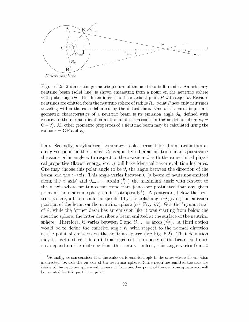
Neutrinosphere
Rν
Θ
ϑ0
ϑϑmax ν
C
A E
I
Pz
Θmax
B
Figure 5.2: 2 dimension geometric picture of the neutrino bulb model. An arbitraryneutrino beam (solid line) is shown emanating from a point on the neutrino spherewith polar angle Θ. This beam intersects the z–axis at point P with angle ϑ. Becauseneutrinos are emitted from the neutrino sphere of radius Rν , point P sees only neutrinostraveling within the cone delimited by the dotted lines. One of the most importantgeometric characteristics of a neutrino beam is its emission angle ϑ0, defined withrespect to the normal direction at the point of emission on the neutrino sphere ϑ0 =Θ+ϑ). All other geometric properties of a neutrino beam may be calculated using theradius r = CP and ϑ0.
here. Secondly, a cylindrical symmetry is also present for the neutrino flux atany given point on the z–axis. Consequently different neutrino beams possessingthe same polar angle with respect to the z–axis and with the same initial physi-cal properties (flavor, energy, etc...) will have identical flavor evolution histories.One may choose this polar angle to be ϑ, the angle between the direction of thebeam and the z–axis. This angle varies between 0 (a beam of neutrinos emittedalong the z–axis) and ϑmax ≡ arcsin
(
Rν
r
)
the maximum angle with respect tothe z–axis where neutrinos can come from (since we postulated that any givenpoint of the neutrino sphere emits isotropically2). A posteriori, below the neu-trino sphere, a beam could be specified by the polar angle Θ giving the emissionposition of the beam on the neutrino sphere (see Fig. 5.2). Θ is the ”symmetric”of ϑ, while the former describes an emission like it was starting from below theneutrino sphere, the latter describes a beam emitted at the surface of the neutrinosphere. Therefore, Θ varies between 0 and Θmax ≡ arcos
(
Rν
r
)
. A third optionwould be to define the emission angle ϑ0 with respect to the normal directionat the point of emission on the neutrino sphere (see Fig. 5.2). That definitionmay be useful since it is an intrinsic geometric property of the beam, and doesnot depend on the distance from the center. Indeed, this angle varies from 0
2Actually, we can consider that the emission is semi-isotropic in the sense where the emissionis directed towards the outside of the neutrinos sphere. Since neutrinos emitted towards theinside of the neutrino sphere will come out from another point of the neutrino sphere and willbe counted for this particular point.
92
(like for other angles, it is when the emission is along the z–axis) and π/2 whichcorresponds to a neutrino emitted in a tangent way at point B on Fig. 5.2. More-over, because of assumptions 1 and 2 in the neutrino bulb model, all the neutrinobeams with the same emission angle ϑ0 and the same initial physical propertiesmust be equivalent. In simulating the flavor transformations of neutrinos in theneutrino bulb model, it is only necessary to follow a group of neutrinos which areuniquely indexed by their initial flavors, energies and emission angles. At anygiven radius r, all the geometric properties of a neutrino beam may be calcu-lated using r and ϑ0. For example, ϑ and Θ are related ϑ0 through the followingidentity:
sinϑ0
r=
sin Θ
l − l0=
sinϑ
Rν, (5.9)
wherel ≡ AP ≡ r cosϑ, (5.10)
andl0 ≡ AE ≡ Rν cosϑ0. (5.11)
The length l − l0 in Eq.(5.9) is also the total propagation distance along theneutrino beam.
The differential number density of neutrinos
The neutrino-neutrino interaction Hamiltonian depends on the probability fora neutrino emitted initially at the neutrino sphere with flavour α to be in acertain flavour β at a certain distance, this probability can be expressed via theelement ρνβνβ
of the density matrix ρνα. Since we are interested in the interaction
between a certain neutrino and the neutrino background with which it interacts,one also has to take into account the set of neutrinos which have the same flavourevolution history describe by ρνβνβ
. Thus, let us now express this set of neutrinosby a differential number density of neutrinos dnνα
(q) at radius r which has thecontribution from all να with energy q which propagate in directions within therange between q and q + dq. The calculation of this differential number is madein appendix D, it leads to:
Hνν =
√2GF
2πR2ν
∑
α
∫
(1− cosϑ cosϑ′) (5.12)
[
ρνα(q′, ϑ′)fνα
(q′)Lνα
〈Eνα〉 − ρ
∗να
(q′, ϑ′)fνα(q′)
Lνα
〈Eνα〉
]
d(cos ϑ′)dq′.
This is the multi-angle neutrino-neutrino interaction Hamiltonian where, in ad-dition to the momentum, we also integrate over the emission angle ϑ′ when weconsider the direction of interaction given by ϑ. Such a computation is numer-ically very demanding, that is why an approximation is often made to obtainmore easily numerical results taking into account the neutrino self-interaction.
93
The single angle approximation
The single angle approximation assumes that the flavor evolution history of aneutrino is trajectory independent. Another way to see it is to consider thatall neutrinos interacting at radius r have been emitted with the same angle.Mathematically, the single angle approximation sums up in the formula :
ρν(q, ϑ) = ρν(q) (5.13)
Neutrinos on any trajectory transform in the same way as neutrinos propagatingin the radial direction that we chose here to be the z–axis3. Consequently, wecan factorized out of the integral the terms proportional to ρνα
(q′) and ρ∗να(q′) in
Eq.(D.15) and it reduces for the spatial dependence to the calculations of :∫
(1− cos ϑ′)d(cos ϑ′) =
∫ 1
cos ϑmax
(1− x)dx
=1
2[1− cosϑmax]
2
=1
2
1−
√
1−(
Rν
r
)2
2
, (5.14)
recalling that ϑmax ≡ arcsin(
Rν
r
)
. Finally, the single-angle self-interaction Hamil-tonian is given by:
Hνν =
√2GF
2πR2ν
D(r/Rν)∑
α
∫
[ρνα(q′)Lνα
(q′)− ρ∗να(q′)Lνα
(q′)]dq′ (5.15)
with the geometrical factor
D(r/Rν) =1
2
1−
√
1−(
Rν
r
)2
2
. (5.16)
In the approximation of large r/Rν , the geometrical factor varies like:
D(r/Rν) ∼1
r4(5.17)
In our supernova model, the matter density is proportional to∼ 1r3 . Consequently,
the strength of the neutrino-neutrino interaction decreases faster than the matterinteraction strength. On Fig.(5.3), one can see the dependence of the matterand the neutrino-neutrino interactions as a function of the distance inside thestar. It also shows the approximative ranges where self-interaction effects areexpected to produce mainly synchronization, bipolar oscillations and a spectralsplit (considering that θ13 is not zero). We now explain to which physical situationcorrespond each of these three stages.
3This means choosing θ = 0
94
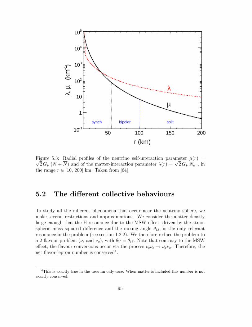
r (km)
50 100 150 200
)-1
(k
mµ, λ
-110
1
10
210
310
410
510
µ
λ
synch bipolar split
Figure 5.3: Radial profiles of the neutrino self-interaction parameter µ(r) =√2GF (N + N) and of the matter-interaction parameter λ(r) =
√2GF Ne−, in
the range r ∈ [10, 200] km. Taken from [64]
5.2 The different collective behaviours
To study all the different phenomena that occur near the neutrino sphere, wemake several restrictions and approximations. We consider the matter densitylarge enough that the H-resonance due to the MSW effect, driven by the atmo-spheric mass squared difference and the mixing angle θ13, is the only relevantresonance in the problem (see section 1.2.2). We therefore reduce the problem toa 2-flavour problem (νe and νx), with θV = θ13. Note that contrary to the MSWeffect, the flavour conversions occur via the process νeνe → νxνx. Therefore, thenet flavor-lepton number is conserved4.
4This is exactly true in the vacuum only case. When matter is included this number is notexactly conserved.
95
5.2.1 The synchronized regime
During the investigation on the neutrino-neutrino interaction that can occur inmedia such as a supernova or the early Universe, people have found that a partic-ular phenomenon can occur when the interactions between neutrinos overcomethe other interactions. Usually, the flavor oscillation of neutrinos depends onthe energy of a given mode, but self-interactions can induce a strong couplingbetween neutrinos in such a way that their flavour oscillations are synchronized.Let us discuss its physical interpretation. In this subsection, concerning the syn-chronized regime, we do not take into account the interactions between neutrinosand matter.
The equation of motion
We use here the formalism of the polarization vectors (appendix C) where theequation of motion for a single mode j is
Pj =∆m2
2pjB×Pj +
√2GF
VJ×Pj, (5.18)
The vector B = (sin 2θV , 0,− cos 2θV ), with the mixing angle θ, can be seen asan effective ”magnetic field” around which P precesses. The total polarizationvector J which represents an ensemble of neutrinos is defined by
J ≡Nν∑
j=1
Pj, (5.19)
where we considered a large volume V filled homogeneously with Nν neutrinos.The first term in the r.h.s of (5.18) shows that P plays the role of an angularmomentum vector and ω is the precession frequency in vacuum of P around B.The second term represents the self interactions. Taken alone on the r.h.s, itmeans that the neutrino j precesses around the total polarization vector J.
The synchronized oscillations
Let us put ourselves in the case where the neutrino density is sufficiently largeso that the vacuum term can be neglected. We follow the analytical derivationsgiven in [95]. Equation (5.18) becomes
Pj =
√2GF
VJ×Pj, (5.20)
From this equation, it is clear that every individual modes precesses around thedirection J. Considering that the density of neutrinos is very large, even byswitching on the vacuum term, the evolution of a given mode remains dominated
96
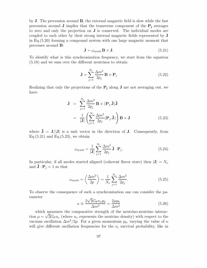
by J. The precession around B, the external magnetic field is slow while the fastprecession around J implies that the transverse component of the Pj averagesto zero and only the projection on J is conserved. The individual modes arecoupled to each other by their strong internal magnetic fields represented by Jin Eq.(5.20) forming a compound system with one large magnetic moment thatprecesses around B:
J = ωsynch B× J. (5.21)
To identify what is this synchronization frequency, we start from the equation(5.18) and we sum over the different neutrinos to obtain:
J =Nν∑
j=1
∆m2
2pj
B×Pj (5.22)
Realizing that only the projections of the Pj along J are not averaging out, wehave:
J =
Nν∑
j=1
∆m2
2pjB× (Pj.J)J
=1
|J|
(
Nν∑
j=1
∆m2
2pj(Pj.J)
)
B× J (5.23)
where J = J/|J| is a unit vector in the direction of J. Consequently, fromEq.(5.21) and Eq.(5.23), we obtain
ωsynch =1
|J|
Nν∑
j=1
∆m2
2pj
J ·Pj. (5.24)
In particular, if all modes started aligned (coherent flavor state) then |J| = Nν
and J ·Pj = 1 so that
ωsynch =
⟨
∆m2
2p
⟩
=1
Nν
Nν∑
j=1
∆m2
2pj. (5.25)
To observe the consequence of such a synchronization one can consider the pa-rameter
κ ≡ 2√
2GFnνp0
∆m2=
2µp0
∆m2(5.26)
which measures the comparative strength of the neutrino-neutrino interac-tion µ =
√2GFnν (where nν represents the neutrino density) with respect to the
vacuum oscillation ∆m2/2p. For a given momentum p0, varying the value of κwill give different oscillation frequencies for the νe survival probability, like in
97
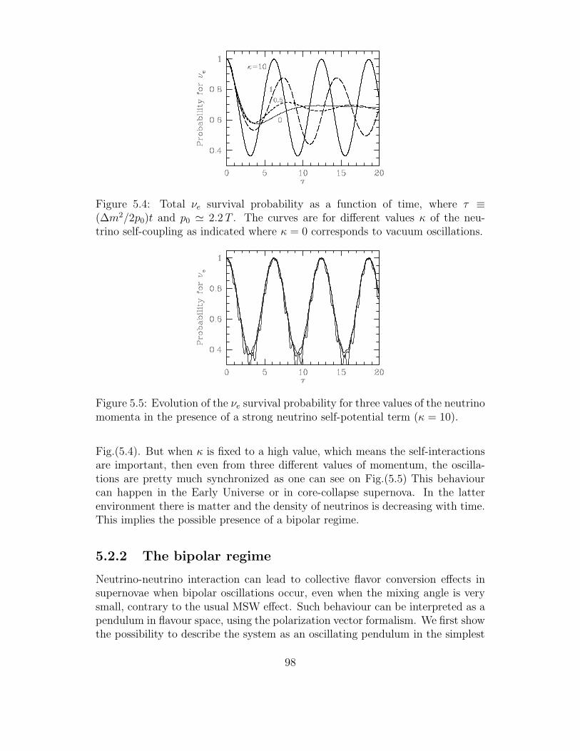
Figure 5.4: Total νe survival probability as a function of time, where τ ≡(∆m2/2p0)t and p0 ≃ 2.2 T . The curves are for different values κ of the neu-trino self-coupling as indicated where κ = 0 corresponds to vacuum oscillations.
Figure 5.5: Evolution of the νe survival probability for three values of the neutrinomomenta in the presence of a strong neutrino self-potential term (κ = 10).
Fig.(5.4). But when κ is fixed to a high value, which means the self-interactionsare important, then even from three different values of momentum, the oscilla-tions are pretty much synchronized as one can see on Fig.(5.5) This behaviourcan happen in the Early Universe or in core-collapse supernova. In the latterenvironment there is matter and the density of neutrinos is decreasing with time.This implies the possible presence of a bipolar regime.
5.2.2 The bipolar regime
Neutrino-neutrino interaction can lead to collective flavor conversion effects insupernovae when bipolar oscillations occur, even when the mixing angle is verysmall, contrary to the usual MSW effect. Such behaviour can be interpreted as apendulum in flavour space, using the polarization vector formalism. We first showthe possibility to describe the system as an oscillating pendulum in the simplest
98
case, and see the consequence of the hierarchy. We then show the influence of thematter on the pendulum behaviour. Finally, we study the system when a morerealistic case is taken, namely with varying neutrino density and with initialneutrino/anti-neutrino asymmetry. We follow the analytical derivations given in[72].
The pendulum model
We consider here the simplest bipolar system, where initially equal densities ofpure νe and νe. In addition, we take all neutrinos to have the same energy, soevery neutrino behave in the same way. We take the exact same notations thatthe ones used in the previous section.
∂tP =[
+ωB + µ(
P− P)]
×P ,
∂tP =[
−ωB + µ(
P− P)]
× P , (5.27)
where P corresponds to the anti-neutrino polarization vector. We then definetwo new variables D and S from P and P:
D = P− P (5.28)
andS = P + P . (5.29)
they are the solution of the new equations of motion:
S = ωB×D + µD× S ,
D = ωB× S . (5.30)
In order to have simpler E.O.M, instead of using S we use
Q = S− ω
µB . (5.31)
which finally yield:
Q = µD×Q ,
D = ωB×Q . (5.32)
since S = Q and B×Q = B× S.Multiplying the E.O.M for Q in Eqs.(5.32), one can see that the squared
modulus of Q is constant and therefore the length of Q is conserved. Using theinitial conditions, namely P(0) = P(0) = (0, 0, 1), we have5:
Q = |Q| =[
4 +
(
ω
µ
)2
+ 4ω
µcos 2θV
]1/2
, (5.33)
5We have used |B|2 = 1, and the initial values |S|2 = 4 and B · S = −2 cos 2θ0.
99
Consequently, the vector Q in flavour space plays the role of a spherical pendulumin that its length is conserved so that it can move only on a sphere of radiusQ. Actually, looking at Eqs.(5.27) and (5.31), we realize that the pendulum’ssubsequent oscillations, represented by the vector Q, are confined in a planedefined by B and the z-axis. Indeed, in vacuum the vectors P and P evolvein the same way except that they rotate in opposite directions, therefore, theirrespective y−component cancels each other. Consequently, the vector Q has onlytwo evolving components on the x− and z− axis. Therefore, we can define Qsuch as:
Q =
sinϕx0y
cosϕz
(5.34)
where ϕ is the tilt angle of Q relative to the z-axis. Finally, the problem variablesare:
ϕ = µD ,
D = −ωQ sin(ϕ+ 2θV ) . (5.35)
Noticing from Eqs.(5.35), that ϕ is a coordinate and D its canonically conjugatemomentum, we can obtain the form of the corresponding Hamiltonian, namely:
H(ϕ,D) =κ2
µ
[
1− cos(ϕ+ 2θV )]
+1
2µD2 = V + T
= ωB ·Q +µ
2D2 , (5.36)
where
κ2 = ωµQ . (5.37)
It corresponds to the motion of a simple pendulum where the first term V =ωB ·Q is the potential energy in a homogeneous field and the second term T =µ2D2/2 is the kinetic energy. We now study the influence of the hierarchy on thependulum behaviour.
The importance of the hierarchy
We first consider the normal hierarchy case and then investigate the invertedhierarchy case. Assuming a small vacuum mixing angle θ0 and a small excursionangle ϕ of the pendulum, the potential can be expanded to the second order:
V (ϕ) = κ2 [1− cos(ϕ+ 2θV )]
=κ2
2(ϕ+ 2θV )2 + . . . . (5.38)
100
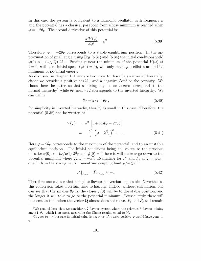
In this case the system is equivalent to a harmonic oscillator with frequency κand the potential has a classical parabolic form whose minimum is reached whenϕ = −2θV . The second derivative of this potential is:
d2V (ϕ)
dϕ2= κ2 (5.39)
Therefore, ϕ = −2θV corresponds to a stable equilibrium position. In the ap-proximation of small angle, using Eqs.(5.31) and (5.34) the initial conditions yieldϕ(0) ≈ −(ω/µQ) 2θV . Putting ϕ near the minimum of the potential V (ϕ) att = 0, with zero initial speed (ϕ(0) = 0), will only make ϕ oscillates around itsminimum of potential energy.As discussed in chapter 1, there are two ways to describe an inverted hierarchy,either we consider a positive cos 2θV and a negative ∆m2 or the contrary. Wechoose here the latter, so that a mixing angle close to zero corresponds to thenormal hierarchy6 while θV near π/2 corresponds to the inverted hierarchy. Wecan define
θV = π/2− θV . (5.40)
for simplicity in inverted hierarchy, thus θV is small in this case. Therefore, thepotential (5.38) can be written as
V (ϕ) = κ2[
1 + cos(ϕ− 2θV )]
= −κ2
2
(
ϕ− 2θV
)2
+ . . . . (5.41)
Here ϕ = 2θV corresponds to the maximum of the potential, and to an unstableequilibrium position. The initial conditions being equivalent to the previousones, i.e ϕ(0) ≈ −(ω/µQ) 2θV and ϕ(0) = 0, here it will make ϕ go down to thepotential minimum where ϕmin ≈ −π7. Evaluating for Pz and Pz at ϕ = ϕmin,one finds in the strong neutrino-neutrino coupling limit µ/ω ≫ 1 :
Pz|ϕmin= Pz|ϕmin
≈ −1 (5.42)
Therefore one can see that complete flavour conversion is possible. Neverthelessthis conversion takes a certain time to happen. Indeed, without calculation, onecan see that the smaller θV is, the closer ϕ(0) will be to the stable position, andthe longer it will take to go to the potential minimum. Consequently there willbe a certain time when the vector Q almost does not move. Pz and Pz will remain
6We remind here that we consider a 2 flavour system where the relevant 3 flavour mixingangle is θ13 which is at most, according tho Chooz results, equal to 9.
7It goes to −π because its initial value is negative, if it were positive ϕ would have gone toπ.
101
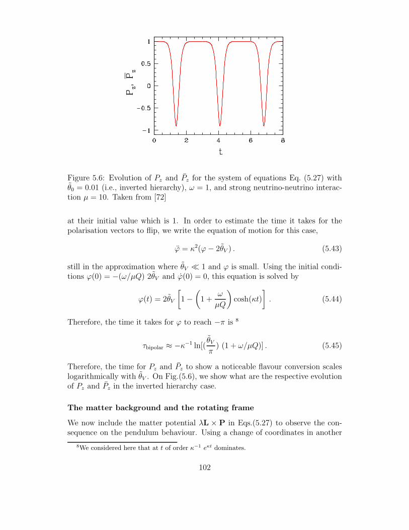
Figure 5.6: Evolution of Pz and Pz for the system of equations Eq. (5.27) withθ0 = 0.01 (i.e., inverted hierarchy), ω = 1, and strong neutrino-neutrino interac-tion µ = 10. Taken from [72]
at their initial value which is 1. In order to estimate the time it takes for thepolarisation vectors to flip, we write the equation of motion for this case,
ϕ = κ2(ϕ− 2θV ) . (5.43)
still in the approximation where θV ≪ 1 and ϕ is small. Using the initial condi-tions ϕ(0) = −(ω/µQ) 2θV and ϕ(0) = 0, this equation is solved by
ϕ(t) = 2θV
[
1−(
1 +ω
µQ
)
cosh(κt)
]
. (5.44)
Therefore, the time it takes for ϕ to reach −π is 8
τbipolar ≈ −κ−1 ln[(θV
π) (1 + ω/µQ)] . (5.45)
Therefore, the time for Pz and Pz to show a noticeable flavour conversion scaleslogarithmically with θV . On Fig.(5.6), we show what are the respective evolutionof Pz and Pz in the inverted hierarchy case.
The matter background and the rotating frame
We now include the matter potential λL × P in Eqs.(5.27) to observe the con-sequence on the pendulum behaviour. Using a change of coordinates in another
8We considered here that at t of order κ−1 eκt dominates.
102
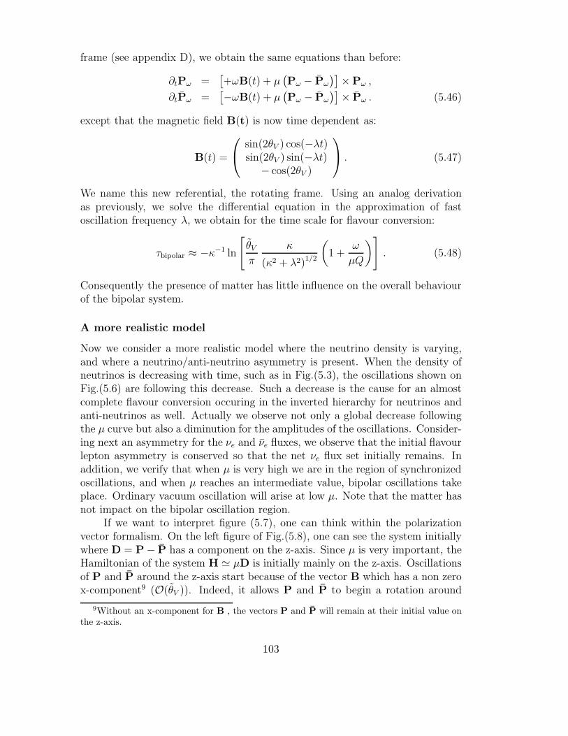
frame (see appendix D), we obtain the same equations than before:
∂tPω =[
+ωB(t) + µ(
Pω − Pω
)]
×Pω ,
∂tPω =[
−ωB(t) + µ(
Pω − Pω
)]
× Pω . (5.46)
except that the magnetic field B(t) is now time dependent as:
B(t) =
sin(2θV ) cos(−λt)sin(2θV ) sin(−λt)− cos(2θV )
. (5.47)
We name this new referential, the rotating frame. Using an analog derivationas previously, we solve the differential equation in the approximation of fastoscillation frequency λ, we obtain for the time scale for flavour conversion:
τbipolar ≈ −κ−1 ln
[
θV
π
κ
(κ2 + λ2)1/2
(
1 +ω
µQ
)
]
. (5.48)
Consequently the presence of matter has little influence on the overall behaviourof the bipolar system.
A more realistic model
Now we consider a more realistic model where the neutrino density is varying,and where a neutrino/anti-neutrino asymmetry is present. When the density ofneutrinos is decreasing with time, such as in Fig.(5.3), the oscillations shown onFig.(5.6) are following this decrease. Such a decrease is the cause for an almostcomplete flavour conversion occuring in the inverted hierarchy for neutrinos andanti-neutrinos as well. Actually we observe not only a global decrease followingthe µ curve but also a diminution for the amplitudes of the oscillations. Consider-ing next an asymmetry for the νe and νe fluxes, we observe that the initial flavourlepton asymmetry is conserved so that the net νe flux set initially remains. Inaddition, we verify that when µ is very high we are in the region of synchronizedoscillations, and when µ reaches an intermediate value, bipolar oscillations takeplace. Ordinary vacuum oscillation will arise at low µ. Note that the matter hasnot impact on the bipolar oscillation region.
If we want to interpret figure (5.7), one can think within the polarizationvector formalism. On the left figure of Fig.(5.8), one can see the system initiallywhere D = P− P has a component on the z-axis. Since µ is very important, theHamiltonian of the system H ≃ µD is initially mainly on the z-axis. Oscillationsof P and P around the z-axis start because of the vector B which has a non zerox-component9 (O(θV )). Indeed, it allows P and P to begin a rotation around
9Without an x-component for B , the vectors P and P will remain at their initial value onthe z-axis.
103
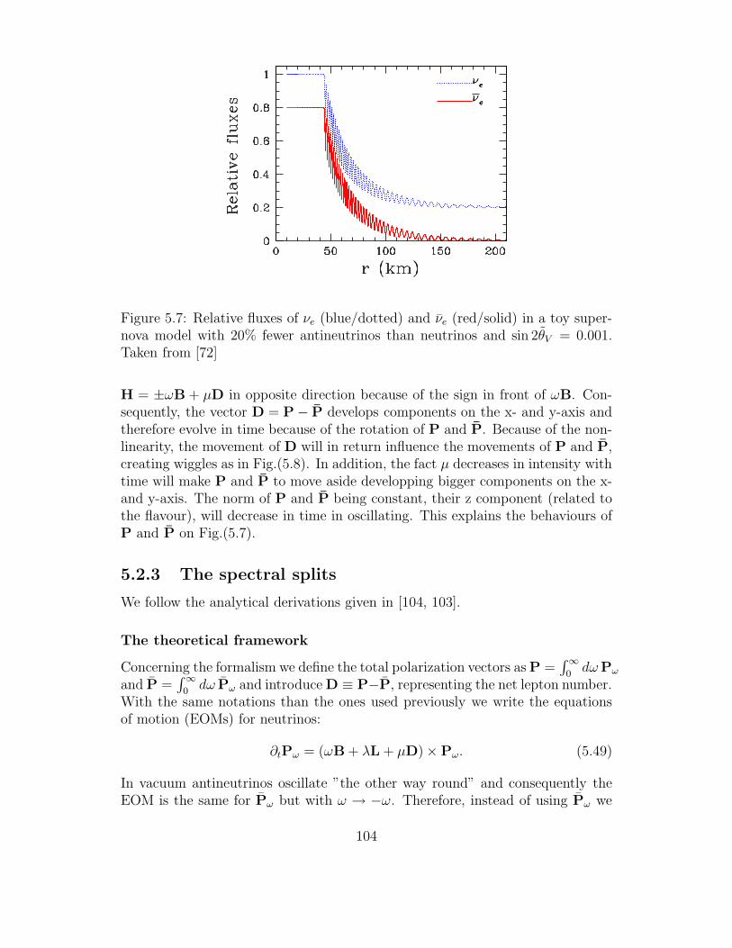
Figure 5.7: Relative fluxes of νe (blue/dotted) and νe (red/solid) in a toy super-nova model with 20% fewer antineutrinos than neutrinos and sin 2θV = 0.001.Taken from [72]
H = ±ωB + µD in opposite direction because of the sign in front of ωB. Con-sequently, the vector D = P− P develops components on the x- and y-axis andtherefore evolve in time because of the rotation of P and P. Because of the non-linearity, the movement of D will in return influence the movements of P and P,creating wiggles as in Fig.(5.8). In addition, the fact µ decreases in intensity withtime will make P and P to move aside developping bigger components on the x-and y-axis. The norm of P and P being constant, their z component (related tothe flavour), will decrease in time in oscillating. This explains the behaviours ofP and P on Fig.(5.7).
5.2.3 The spectral splits
We follow the analytical derivations given in [104, 103].
The theoretical framework
Concerning the formalism we define the total polarization vectors as P =∫∞0dωPω
and P =∫∞0dω Pω and introduce D ≡ P−P, representing the net lepton number.
With the same notations than the ones used previously we write the equationsof motion (EOMs) for neutrinos:
∂tPω = (ωB + λL + µD)×Pω. (5.49)
In vacuum antineutrinos oscillate ”the other way round” and consequently theEOM is the same for Pω but with ω → −ω. Therefore, instead of using Pω we
104
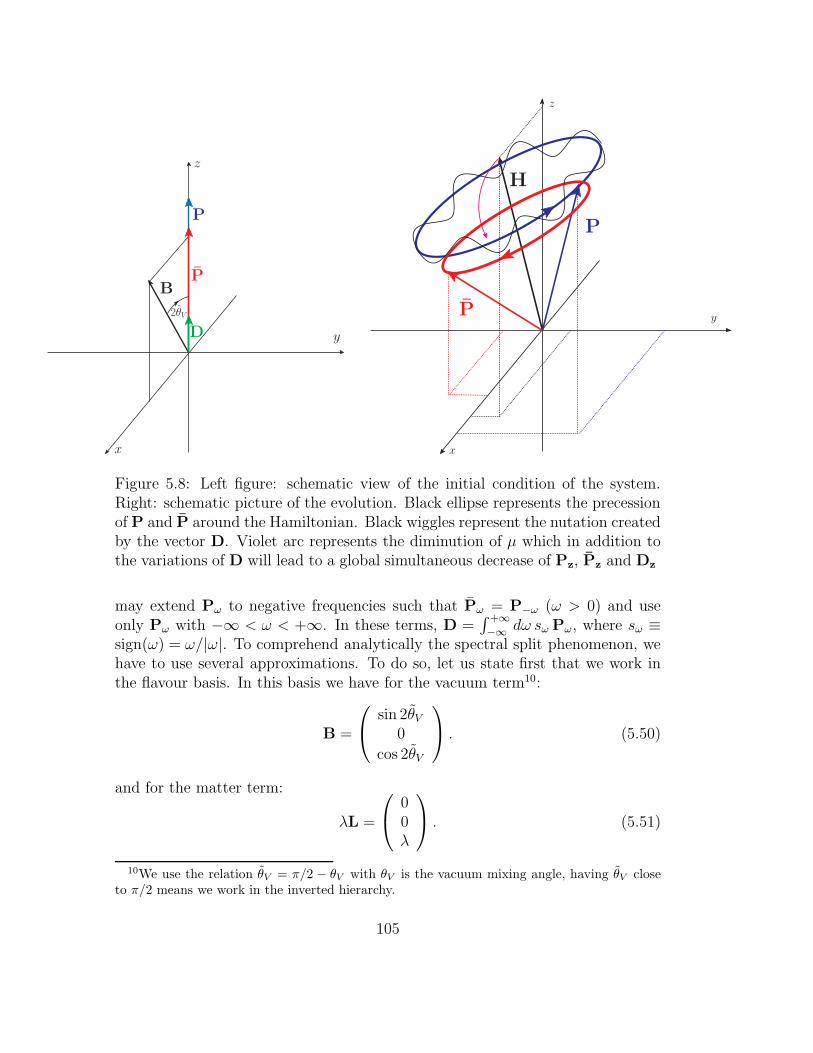
D
P
BP
x
y
z
2θV
x
y
z
P
P
H
Figure 5.8: Left figure: schematic view of the initial condition of the system.Right: schematic picture of the evolution. Black ellipse represents the precessionof P and P around the Hamiltonian. Black wiggles represent the nutation createdby the vector D. Violet arc represents the diminution of µ which in addition tothe variations of D will lead to a global simultaneous decrease of Pz, Pz and Dz
may extend Pω to negative frequencies such that Pω = P−ω (ω > 0) and useonly Pω with −∞ < ω < +∞. In these terms, D =
∫ +∞−∞ dω sω Pω, where sω ≡
sign(ω) = ω/|ω|. To comprehend analytically the spectral split phenomenon, wehave to use several approximations. To do so, let us state first that we work inthe flavour basis. In this basis we have for the vacuum term10:
B =
sin 2θV
0
cos 2θV
. (5.50)
and for the matter term:
λL =
00λ
. (5.51)
10We use the relation θV = π/2 − θV with θV is the vacuum mixing angle, having θV closeto π/2 means we work in the inverted hierarchy.
105
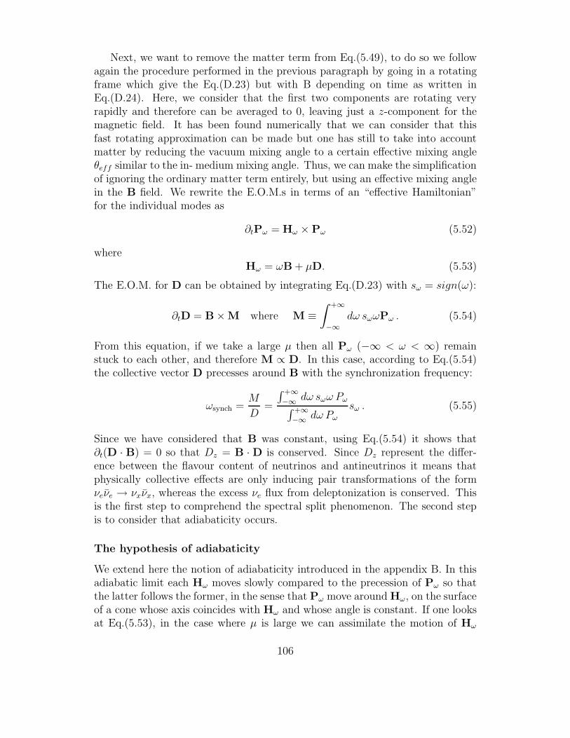
Next, we want to remove the matter term from Eq.(5.49), to do so we followagain the procedure performed in the previous paragraph by going in a rotatingframe which give the Eq.(D.23) but with B depending on time as written inEq.(D.24). Here, we consider that the first two components are rotating veryrapidly and therefore can be averaged to 0, leaving just a z-component for themagnetic field. It has been found numerically that we can consider that thisfast rotating approximation can be made but one has still to take into accountmatter by reducing the vacuum mixing angle to a certain effective mixing angleθeff similar to the in- medium mixing angle. Thus, we can make the simplificationof ignoring the ordinary matter term entirely, but using an effective mixing anglein the B field. We rewrite the E.O.M.s in terms of an “effective Hamiltonian”for the individual modes as
∂tPω = Hω ×Pω (5.52)
whereHω = ωB + µD. (5.53)
The E.O.M. for D can be obtained by integrating Eq.(D.23) with sω = sign(ω):
∂tD = B×M where M ≡∫ +∞
−∞dω sωωPω . (5.54)
From this equation, if we take a large µ then all Pω (−∞ < ω < ∞) remainstuck to each other, and therefore M ∝ D. In this case, according to Eq.(5.54)the collective vector D precesses around B with the synchronization frequency:
ωsynch =M
D=
∫ +∞−∞ dω sωω Pω∫ +∞−∞ dω Pω
sω . (5.55)
Since we have considered that B was constant, using Eq.(5.54) it shows that∂t(D · B) = 0 so that Dz = B · D is conserved. Since Dz represent the differ-ence between the flavour content of neutrinos and antineutrinos it means thatphysically collective effects are only inducing pair transformations of the formνeνe → νxνx, whereas the excess νe flux from deleptonization is conserved. Thisis the first step to comprehend the spectral split phenomenon. The second stepis to consider that adiabaticity occurs.
The hypothesis of adiabaticity
We extend here the notion of adiabaticity introduced in the appendix B. In thisadiabatic limit each Hω moves slowly compared to the precession of Pω so thatthe latter follows the former, in the sense that Pω move around Hω, on the surfaceof a cone whose axis coincides with Hω and whose angle is constant. If one looksat Eq.(5.53), in the case where µ is large we can assimilate the motion of Hω
106
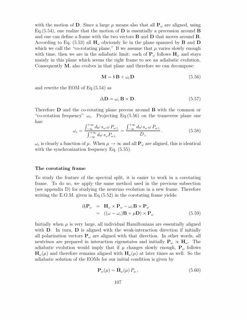
with the motion of D. Since a large µ means also that all Pω are aligned, usingEq.(5.54), one realize that the motion of D is essentially a precession around Band one can define a frame with the two vectors B and D that moves around B.According to Eq. (5.53) all Hω obviously lie in the plane spanned by B and Dwhich we call the “co-rotating plane.” If we assume that µ varies slowly enoughwith time, then we are in the adiabatic limit: each of Pω follows Hω and staysmainly in this plane which seems the right frame to see an adiabatic evolution.Consequently M, also evolves in that plane and therefore we can decompose:
M = bB + ωcD (5.56)
and rewrite the EOM of Eq.(5.54) as
∂tD = ωc B×D. (5.57)
Therefore D and the co-rotating plane precess around B with the common or“co-rotation frequency” ωc. Projecting Eq.(5.56) on the transverse plane onehas:
ωc =
∫ +∞−∞ dω sω ω Pω⊥∫ +∞−∞ dω sωPω⊥
=
∫ +∞−∞ dω sω ω Pω⊥
D⊥. (5.58)
ωc is clearly a function of µ. When µ→∞ and all Pω are aligned, this is identicalwith the synchronization frequency Eq. (5.55).
The corotating frame
To study the feature of the spectral split, it is easier to work in a corotatingframe. To do so, we apply the same method used in the previous subsection(see appendix D) for studying the neutrino evolution in a new frame. Thereforewriting the E.O.M. given in Eq.(5.52) in the corotating frame yields:
∂tPω = Hω ×Pω − ωcB×Pω
= ((ω − ωc)B + µD)×Pω (5.59)
Initially when µ is very large, all individual Hamiltonians are essentially alignedwith D. In turn, D is aligned with the weak-interaction direction if initiallyall polarization vectors Pω are aligned with that direction. In other words, allneutrinos are prepared in interaction eigenstates and initially Pω ∝ Hω. Theadiabatic evolution would imply that if µ changes slowly enough, Pω followsHω(µ) and therefore remains aligned with Hω(µ) at later times as well. So theadiabatic solution of the EOMs for our initial condition is given by
Pω(µ) = Hω(µ)Pω , (5.60)
107
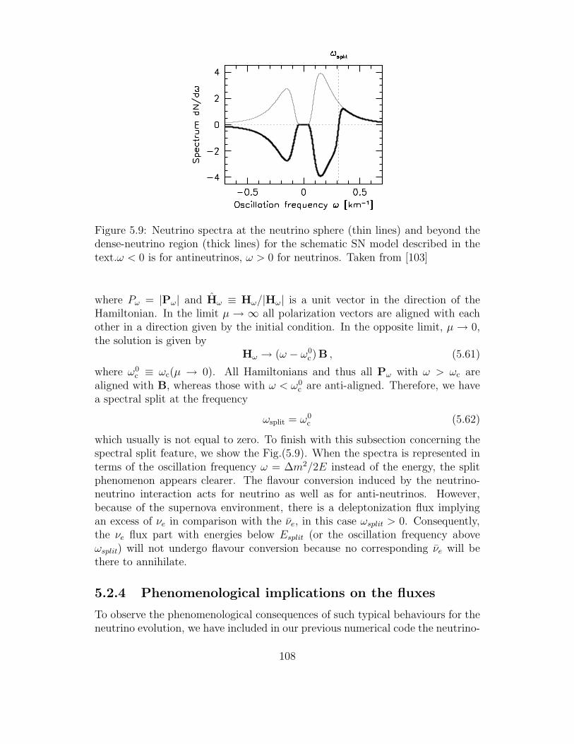
Figure 5.9: Neutrino spectra at the neutrino sphere (thin lines) and beyond thedense-neutrino region (thick lines) for the schematic SN model described in thetext.ω < 0 is for antineutrinos, ω > 0 for neutrinos. Taken from [103]
where Pω = |Pω| and Hω ≡ Hω/|Hω| is a unit vector in the direction of theHamiltonian. In the limit µ → ∞ all polarization vectors are aligned with eachother in a direction given by the initial condition. In the opposite limit, µ → 0,the solution is given by
Hω → (ω − ω0c)B , (5.61)
where ω0c ≡ ωc(µ → 0). All Hamiltonians and thus all Pω with ω > ωc are
aligned with B, whereas those with ω < ω0c are anti-aligned. Therefore, we have
a spectral split at the frequency
ωsplit = ω0c (5.62)
which usually is not equal to zero. To finish with this subsection concerning thespectral split feature, we show the Fig.(5.9). When the spectra is represented interms of the oscillation frequency ω = ∆m2/2E instead of the energy, the splitphenomenon appears clearer. The flavour conversion induced by the neutrino-neutrino interaction acts for neutrino as well as for anti-neutrinos. However,because of the supernova environment, there is a deleptonization flux implyingan excess of νe in comparison with the νe, in this case ωsplit > 0. Consequently,the νe flux part with energies below Esplit (or the oscillation frequency aboveωsplit) will not undergo flavour conversion because no corresponding νe will bethere to annihilate.
5.2.4 Phenomenological implications on the fluxes
To observe the phenomenological consequences of such typical behaviours for theneutrino evolution, we have included in our previous numerical code the neutrino-
108
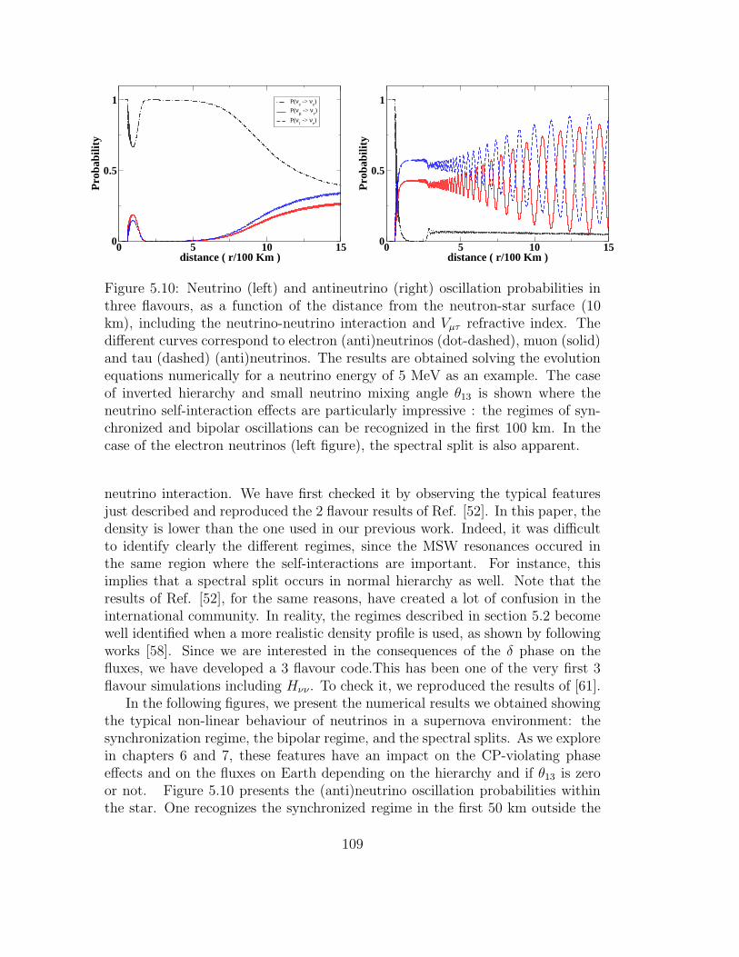
0 5 10 15distance ( r/100 Km )
0
0.5
1P
roba
bilit
y P(ν
e -> ν
e)
P(νµ -> νe)
P(ντ -> νe)
0 5 10 15distance ( r/100 Km )
0
0.5
1
Pro
babi
lity
Figure 5.10: Neutrino (left) and antineutrino (right) oscillation probabilities inthree flavours, as a function of the distance from the neutron-star surface (10km), including the neutrino-neutrino interaction and Vµτ refractive index. Thedifferent curves correspond to electron (anti)neutrinos (dot-dashed), muon (solid)and tau (dashed) (anti)neutrinos. The results are obtained solving the evolutionequations numerically for a neutrino energy of 5 MeV as an example. The caseof inverted hierarchy and small neutrino mixing angle θ13 is shown where theneutrino self-interaction effects are particularly impressive : the regimes of syn-chronized and bipolar oscillations can be recognized in the first 100 km. In thecase of the electron neutrinos (left figure), the spectral split is also apparent.
neutrino interaction. We have first checked it by observing the typical featuresjust described and reproduced the 2 flavour results of Ref. [52]. In this paper, thedensity is lower than the one used in our previous work. Indeed, it was difficultto identify clearly the different regimes, since the MSW resonances occured inthe same region where the self-interactions are important. For instance, thisimplies that a spectral split occurs in normal hierarchy as well. Note that theresults of Ref. [52], for the same reasons, have created a lot of confusion in theinternational community. In reality, the regimes described in section 5.2 becomewell identified when a more realistic density profile is used, as shown by followingworks [58]. Since we are interested in the consequences of the δ phase on thefluxes, we have developed a 3 flavour code.This has been one of the very first 3flavour simulations including Hνν . To check it, we reproduced the results of [61].
In the following figures, we present the numerical results we obtained showingthe typical non-linear behaviour of neutrinos in a supernova environment: thesynchronization regime, the bipolar regime, and the spectral splits. As we explorein chapters 6 and 7, these features have an impact on the CP-violating phaseeffects and on the fluxes on Earth depending on the hierarchy and if θ13 is zeroor not. Figure 5.10 presents the (anti)neutrino oscillation probabilities withinthe star. One recognizes the synchronized regime in the first 50 km outside the
109
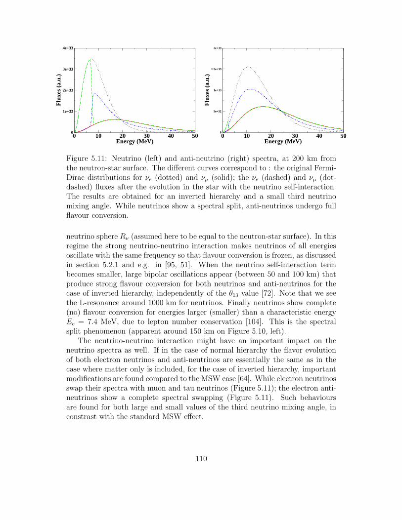
0 10 20 30 40 50Energy (MeV)
0
1e+33
2e+33
3e+33
4e+33
Flu
xes
(a.u
.)
0 10 20 30 40 50Energy (MeV)
0
5e+32
1e+33
1.5e+33
2e+33
Flu
xes
(a.u
.)
Figure 5.11: Neutrino (left) and anti-neutrino (right) spectra, at 200 km fromthe neutron-star surface. The different curves correspond to : the original Fermi-Dirac distributions for νe (dotted) and νµ (solid); the νe (dashed) and νµ (dot-dashed) fluxes after the evolution in the star with the neutrino self-interaction.The results are obtained for an inverted hierarchy and a small third neutrinomixing angle. While neutrinos show a spectral split, anti-neutrinos undergo fullflavour conversion.
neutrino sphere Rν (assumed here to be equal to the neutron-star surface). In thisregime the strong neutrino-neutrino interaction makes neutrinos of all energiesoscillate with the same frequency so that flavour conversion is frozen, as discussedin section 5.2.1 and e.g. in [95, 51]. When the neutrino self-interaction termbecomes smaller, large bipolar oscillations appear (between 50 and 100 km) thatproduce strong flavour conversion for both neutrinos and anti-neutrinos for thecase of inverted hierarchy, independently of the θ13 value [72]. Note that we seethe L-resonance around 1000 km for neutrinos. Finally neutrinos show complete(no) flavour conversion for energies larger (smaller) than a characteristic energyEc = 7.4 MeV, due to lepton number conservation [104]. This is the spectralsplit phenomenon (apparent around 150 km on Figure 5.10, left).
The neutrino-neutrino interaction might have an important impact on theneutrino spectra as well. If in the case of normal hierarchy the flavor evolutionof both electron neutrinos and anti-neutrinos are essentially the same as in thecase where matter only is included, for the case of inverted hierarchy, importantmodifications are found compared to the MSW case [64]. While electron neutrinosswap their spectra with muon and tau neutrinos (Figure 5.11); the electron anti-neutrinos show a complete spectral swapping (Figure 5.11). Such behavioursare found for both large and small values of the third neutrino mixing angle, inconstrast with the standard MSW effect.
110
Chapter 6
Collective neutrino oscillations insupernovae and CP-violation
Motivated by the important recent developments in the study of neutrino propa-gation in dense media, due in particular to the inclusion of the neutrino-neutrinointeraction and the emergence of new collective neutrino flavour conversion phe-nomena (described in chapter 4), we have explored the robustness of the analyticaland numerical results found in the standard framework of neutrino propagationin matter (the MSW effect) when the neutrino self-interactions are present [69].
6.1 Analytical results
Since we are dealing with the neutrino-neutrino interaction, it is more convenientto write the equation of motion with the density matrix formalism (see appendixC for details).
Theoretical framework
Considering here the density matrix, the neutrino evolution equation governedby the Liouville-Von Neumann equation is:
idρνα
(δ)
dt= [UHvacU
† +Hm +Hνν(δ), ρνα(δ)], (6.1)
where the neutrino-neutrino interaction term is:
Hνν =
√2GF
2πR2ν
D(r/Rν)∑
α
∫
[ρνα(q′)Lνα
(q′)− ρ∗να(q′)Lνα
(q′)]dq′ (6.2)
with the geometrical factor
D(r/Rν) =1
2[1−
√
1− (Rν
r)2]2 (6.3)
111
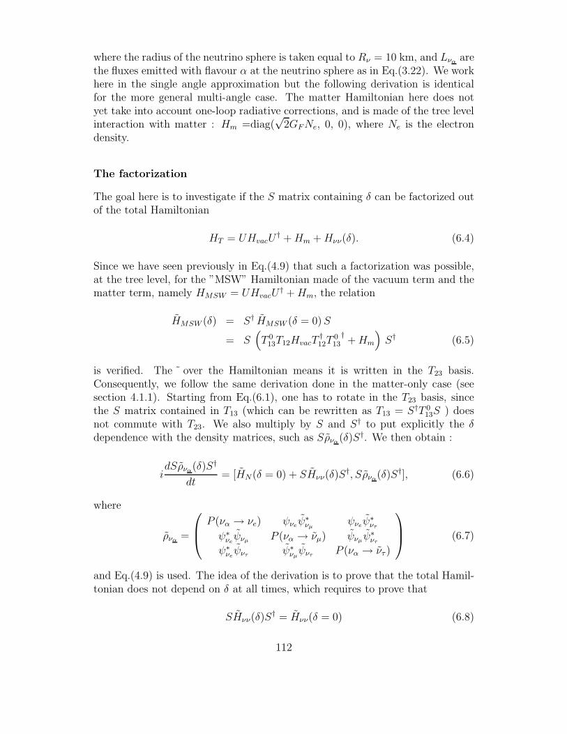
where the radius of the neutrino sphere is taken equal to Rν = 10 km, and Lναare
the fluxes emitted with flavour α at the neutrino sphere as in Eq.(3.22). We workhere in the single angle approximation but the following derivation is identicalfor the more general multi-angle case. The matter Hamiltonian here does notyet take into account one-loop radiative corrections, and is made of the tree levelinteraction with matter : Hm =diag(
√2GFNe, 0, 0), where Ne is the electron
density.
The factorization
The goal here is to investigate if the S matrix containing δ can be factorized outof the total Hamiltonian
HT = UHvacU† +Hm +Hνν(δ). (6.4)
Since we have seen previously in Eq.(4.9) that such a factorization was possible,at the tree level, for the ”MSW” Hamiltonian made of the vacuum term and thematter term, namely HMSW = UHvacU
† +Hm, the relation
HMSW (δ) = S† HMSW (δ = 0)S
= S(
T 013T12HvacT
†12T
013
†+Hm
)
S† (6.5)
is verified. The ˜ over the Hamiltonian means it is written in the T23 basis.Consequently, we follow the same derivation done in the matter-only case (seesection 4.1.1). Starting from Eq.(6.1), one has to rotate in the T23 basis, sincethe S matrix contained in T13 (which can be rewritten as T13 = S†T 0
13S ) doesnot commute with T23. We also multiply by S and S† to put explicitly the δdependence with the density matrices, such as Sρνα
(δ)S†. We then obtain :
idSρνα
(δ)S†
dt= [HN(δ = 0) + SHνν(δ)S
†, Sρνα(δ)S†], (6.6)
where
ρνα=
P (να → νe) ψνeψ∗
νµψνe
ψ∗ντ
ψ∗νeψνµ
P (να → νµ) ψνµψ∗
ντ
ψ∗νeψντ
ψ∗νµψντ
P (να → ντ )
(6.7)
and Eq.(4.9) is used. The idea of the derivation is to prove that the total Hamil-tonian does not depend on δ at all times, which requires to prove that
SHνν(δ)S† = Hνν(δ = 0) (6.8)
112
The proof
The neutrino-neutrino interaction Hamiltonian, Hνν , depends on Sρνα(δ)S† (see
Eqs.(6.1) and (6.2)) which is also the unknown of the problem, making the evo-lution equations non-linear. The subtlety is that such terms are summed overthe different initial conditions in Hνν , since initially either a νe, a νµ, or a ντ areproduced. The terms Sρνα
(δ)S† are calculated for one initial condition να only.Since we wish to prove Eq.(6.8), we consider the evolution equation of the linearcombination B(q, δ) =
∑
ναLνα
Sρνα(q, δ)S† at a given momentum q:
id
dt
(
∑
να
LναSρνα
(q, δ)S†
)
= [HMSW (δ = 0) + SHνν(δ)S†,∑
να
LναSρνα
(q, δ)S†].
(6.9)The second key point of this derivation is to look at the initial conditions. At
the initial time, B(q, δ) reads, in the T23 basis of Eq.(4.6), as :
∑
να
LναSρνα
(q, δ, t = 0)S† =
Lνe0 0
0 c223Lνµ+ s2
23Lντc23s23e
−iδ(Lνµ− Lντ
)
0 c23s23eiδ(Lνµ
− Lντ) s2
23Lνµ+ c223Lντ
(6.10)One immediately sees that B(q, δ, t = 0) does not depend on δ if and only if Lνµ
=
Lντ. The quantity
(
∑
ναLνα
S†ρνα(q, δ, t = 0)S
)∗, which corresponds to the anti-
neutrinos does not depend on δ as well, if and only if Lνµ= Lντ
. Moreover, the
total Hamiltonian HT is independent of δ at initial time since HMSW (δ) does notdepend on δ (at any time) at tree level, and
SHνν(t = 0, δ)S† = (6.11)√
2GF
∑
α
∫
(1− q · q′)[Sρνα(t = 0, q′)S†Lνα
(q′)− Sρ∗να(t = 0, q′)S†Lνα
(q′)]dq′
is equal to Hνν(t = 0, δ = 0) initially when Lνµ= Lντ
(and Lνµ= Lντ
). Inthat case, one can see, by recurrence, from the Liouville-Von Neumann equationEq.(6.9), that the evolution of the term
∑
ναLνα
Sρνα(q, δ)S† is exactly the same
as the term∑
ναLνα
ρνα(q, δ = 0), since they have the same initial conditions
(for any q) and the same evolution equations. Moreover, the exact same relationapplying in the same time for anti-neutrinos (Eq.(6.2)) (but with an oppositesign of δ), one simultaneously obtains that at any time:
Hνν(δ) = SHνν(δ = 0)S†, (6.12)
hence :HT (δ) = SHT (δ = 0)S†. (6.13)
113
Note that the derivation holds both for the multi-angle case Eq.(D.15) and thesingle-angle case Eq.(5.15). This implies that the electron (anti-)neutrino survivalprobability is independent of δ, therefore φνe
(δ) = φνe(δ = 0) and φνe
(δ) =φνe
(δ = 0), even considering the presence of the neutrino-neutrino interaction,if muon and tau neutrino fluxes at the neutrino sphere are equal. When thefluxes Lνµ
and Lντare different, the derivation does not hold anymore, since
∑
ναLνα
Sρνα(q, δ)S† initially depends on δ.
6.2 General condition for CP-violation in super-
novae
Thanks to chapter 4 and the previous section, we are able to draw a clear picturefor the conditions to obtain CP-violation effects on the electron (anti-) neutrinosurvival probability and consequently, on the electron (anti-) neutrino flux. Inthis section, we present a summary for these conditions.
1. When the one loop corrections and the neutrino-neutrino interaction Hamil-tonian (Hνν) are not taken into account for the neutrino propagation beyondthe neutrino sphere (HT = HMSW ), the effects of δ can only manifest if themuon and tau neutrino fluxes are taken different at the neutrino sphere.Such a difference could come from loop corrections and/or from physics be-yond the Standard Model, like the flavour changing neutral current whichcan be introduced via the breaking of the R-parity.
2. When Hνν is added to the evolution equation (HT = HMSW + Hνν), butnot loop corrections, we will also observe CP-effects only if the νµ andντ fluxes are different at the neutrino sphere. With such conditions, thedifference with the previous case is that the factorization of δ out of the totalHamiltonian is not possible anymore. The CP-violation effects will appearnot only on the electron neutrino (resp. electron anti-neutrino) flux butalso on the electron survival probability P (νe → νe, δ) (resp.P (νe → νe, δ)).
3. When only the one loop corrections are added to the evolution equation(HT = HMSW + diag(0, 0, Vµτ)), the matter Hamiltonian cannot be factor-ized anymore, and the δ effects will appear on the fluxes only due to thefact that P (νe → νe, δ) depends on δ.
4. When all interactions mentioned above are added1, (HT = HMSW+diag(0, 0, Vµτ)+Hνν), which is the most realistic case, P (νe → νe, δ) and φνe
depend on δ.
1Note that the possible inclusion of nonstandard neutrino interactions in the flavour neutrinomixing as e.g. in [59] implies that Eq.(9) does not hold anymore.
114
The main problem is to know by how much the νµ and ντ fluxes are differentat the neutrino sphere. Unfortunately, a realistic numerical simulation thatgives an estimate of the difference has never been performed so far.
6.3 Numerical results
The main goal of this section is to investigate numerically the effects that canarise when the factorization Eq.(6.8) is not satisfied, by varying δ ∈ [0, 180]while we show results for δ = 180 when at such value the effects are maximal.Following section 6.2, the results that we present here correspond to the followingpossibilities:
a) Hνν 6= 0 and Vµτ = 0 with the condition Lνµ6= Lντ
;
b) Hνν 6= 0 and Vµτ 6= 0 with the condition Lνµ= Lντ
;
c) Hνν 6= 0 and Vµτ 6= 0 with the condition Lνµ6= Lντ
.
The evolution equation
We decided to use the wave functions formalism in our numerical code since sucha code had been developed for the MSW case (Chapter 4). Note that, in such aformalism, the writing of the neutrino-neutrino interaction Hamiltonian is morecomplicated. As we know the ν − ν interaction Hamiltonian consists of diagonalterms but also of terms that are off-diagonal, which are mainly responsible forthe new conversion behaviours,
Hνν =
HνeνeHνeνµ
Hνeντ
HνµνeHνµνµ
Hνµντ
HντνeHντ νµ
Hντντ
. (6.14)
We can rewrite Hνν as
Hνν = D(r/Rν)
∫
[
Nνe+Nνµ
+Nντ
]
dq′ (6.15)
The different terms Nναin the Hamiltonian Hνν correspond to different initial
conditions since in the supernova, all neutrino flavours are created initially and
115
we have to take them all into account. Let’s make explicit Nνefor instance :
∫
Nνe(q′)dq′ =
∫
(
Lνe(q′)ψe,eψ
∗e,e − Lνe
(q′)ψ∗e,eψe,e
)
dq′
∫
(
Lνe(q′)ψµ,eψ
∗e,e − Lνe
(q′)ψ∗µ,eψe,e
)
dq′
∫
(
Lνe(q′)ψτ,eψ
∗e,e − Lνe
(q′)ψ∗τ,eψe,e
)
dq′
∫
(
Lνe(q′)ψe,eψ
∗µ,e − Lνe
(q′)ψ∗e,eψµ,e
)
dq′
∫
(
Lνe(q′)ψµ,eψ
∗µ,e − Lνe
(q′)ψ∗µ,eψµ,e
)
dq′
∫
(
Lνe(q′)ψτ,eψ
∗µ,e − Lνe
(q′)ψ∗τ,eψµ,e
)
dq′
∫
(
Lνe(q′)ψe,eψ
∗τ,e − Lνe
(q′)ψ∗e,eψτ,e
)
dq′
∫
(
Lνe(q′)ψµ,eψ
∗τ,e − Lνe
(q′)ψ∗µ,eψτ,e
)
dq′
∫
(
Lνe(q′)ψτ,eψ
∗τ,e − Lνe
(q′)ψ∗τ,eψτ,e
)
dq′
(6.16)
The subscript for the wave functions means respectively, the neutrino flavourconsidered, and the initial neutrino flavour at the neutrinosphere.
The input parameters
The numerical results we present are obtained by solving the three flavour evolu-tion equation of Eq.(6.1) with a supernova density profile for which the region ofthe first 100 km, where the neutrino self-interaction dominates, is well separatedfrom the one of the MSW (high and low) resonances, produced by the interactionwith ordinary matter. The oscillation parameters and the neutrino fluxes at theneutrinosphere are the same as the one used in chapter 4. We take the neutrinoluminosity L0
να= 1051 erg · s−1. To include the neutrino-neutrino interaction we
use the single-angle approximation of Eqs.(5.15-5.16) with Rν = 10 km, consid-ering that all neutrinos are emitted radially.Our numerical results in three flavours present the collective oscillations inducedby the neutrino-neutrino interaction, already discussed in the literature (see e.g.[105, 108, 95, 54, 72, 104, 103, 61]) and in the previous chapter.Let us now discuss the CP violation effects in presence of the neutrino-neutrinointeraction2 and of the loop corrections to the neutrino refractive index, withthe condition that the muon and tau fluxes at the neutrinosphere are equal(Lνµ
= Lντ).
2Note that a comment is made in [53, 55] on the δ effects on the neutrino fluxes in thepresence of the neutrino self-interaction in a core-collapse supernova.
116
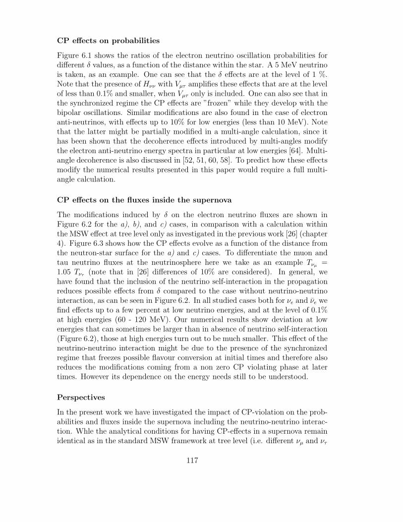
CP effects on probabilities
Figure 6.1 shows the ratios of the electron neutrino oscillation probabilities fordifferent δ values, as a function of the distance within the star. A 5 MeV neutrinois taken, as an example. One can see that the δ effects are at the level of 1 %.Note that the presence of Hνν with Vµτ amplifies these effects that are at the levelof less than 0.1% and smaller, when Vµτ only is included. One can also see that inthe synchronized regime the CP effects are ”frozen” while they develop with thebipolar oscillations. Similar modifications are also found in the case of electronanti-neutrinos, with effects up to 10% for low energies (less than 10 MeV). Notethat the latter might be partially modified in a multi-angle calculation, since ithas been shown that the decoherence effects introduced by multi-angles modifythe electron anti-neutrino energy spectra in particular at low energies [64]. Multi-angle decoherence is also discussed in [52, 51, 60, 58]. To predict how these effectsmodify the numerical results presented in this paper would require a full multi-angle calculation.
CP effects on the fluxes inside the supernova
The modifications induced by δ on the electron neutrino fluxes are shown inFigure 6.2 for the a), b), and c) cases, in comparison with a calculation withinthe MSW effect at tree level only as investigated in the previous work [26] (chapter4). Figure 6.3 shows how the CP effects evolve as a function of the distance fromthe neutron-star surface for the a) and c) cases. To differentiate the muon andtau neutrino fluxes at the neutrinosphere here we take as an example Tνµ
=1.05 Tντ
(note that in [26] differences of 10% are considered). In general, wehave found that the inclusion of the neutrino self-interaction in the propagationreduces possible effects from δ compared to the case without neutrino-neutrinointeraction, as can be seen in Figure 6.2. In all studied cases both for νe and νe wefind effects up to a few percent at low neutrino energies, and at the level of 0.1%at high energies (60 - 120 MeV). Our numerical results show deviation at lowenergies that can sometimes be larger than in absence of neutrino self-interaction(Figure 6.2), those at high energies turn out to be much smaller. This effect of theneutrino-neutrino interaction might be due to the presence of the synchronizedregime that freezes possible flavour conversion at initial times and therefore alsoreduces the modifications coming from a non zero CP violating phase at latertimes. However its dependence on the energy needs still to be understood.
Perspectives
In the present work we have investigated the impact of CP-violation on the prob-abilities and fluxes inside the supernova including the neutrino-neutrino interac-tion. Whle the analytical conditions for having CP-effects in a supernova remainidentical as in the standard MSW framework at tree level (i.e. different νµ and ντ
117
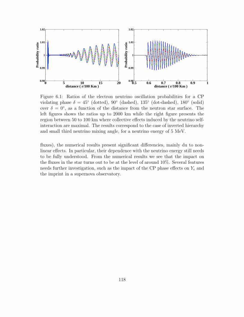
0 5 10 15 20distance ( r/100 Km )
0.98
0.99
1
1.01
1.02
Pro
babi
lity
rati
o
0.5 0.6 0.7 0.8 0.9 1distance ( r/100 Km )
0.98
0.99
1
1.01
1.02
Pro
babi
lity
rati
o
Figure 6.1: Ratios of the electron neutrino oscillation probabilities for a CPviolating phase δ = 45 (dotted), 90 (dashed), 135 (dot-dashed), 180 (solid)over δ = 0, as a function of the distance from the neutron star surface. Theleft figures shows the ratios up to 2000 km while the right figure presents theregion between 50 to 100 km where collective effects induced by the neutrino self-interaction are maximal. The results correspond to the case of inverted hierarchyand small third neutrino mixing angle, for a neutrino energy of 5 MeV.
fluxes), the numerical results present significant differencies, mainly du to non-linear effects. In particular, their dependence with the neutrino energy still needsto be fully understood. From the numerical results we see that the impact onthe fluxes in the star turns out to be at the level of around 10%. Several featuresneeds further investigation, such as the impact of the CP phase effects on Ye andthe imprint in a supernova observatory.
118
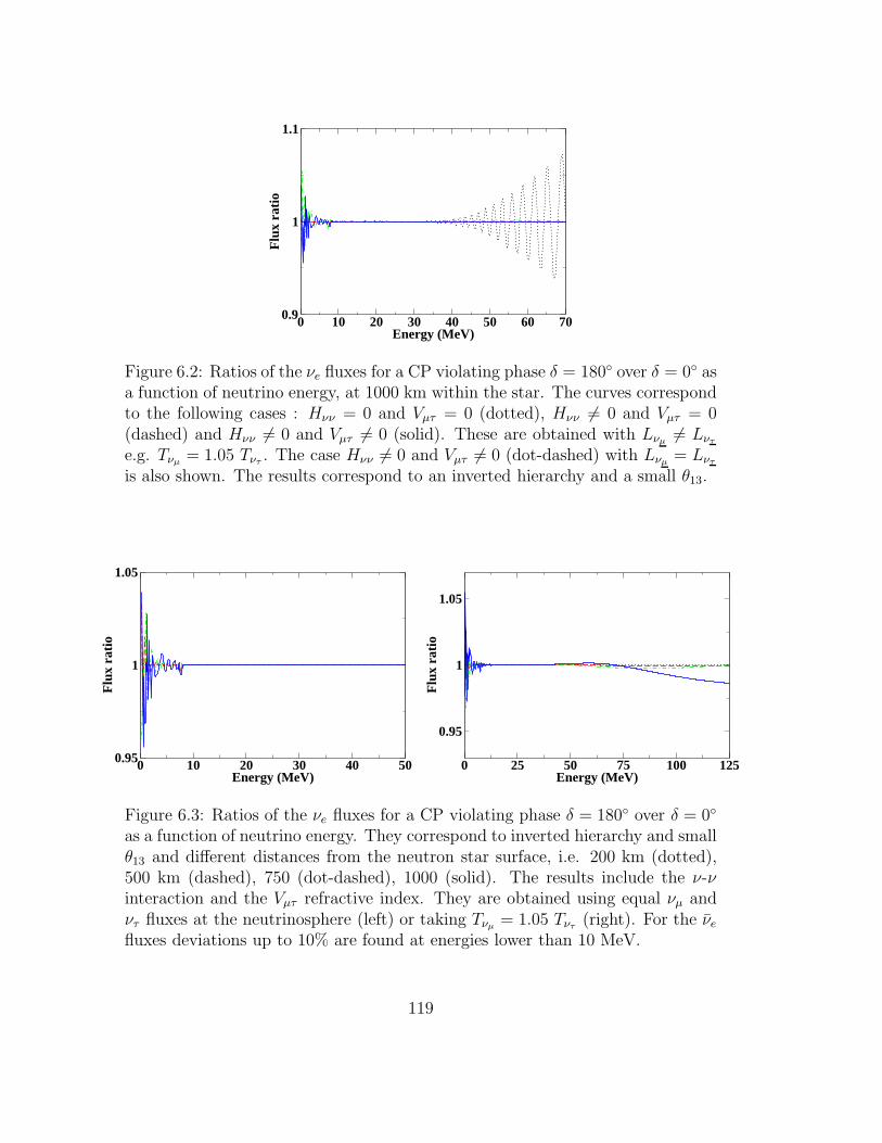
0 10 20 30 40 50 60 70Energy (MeV)
0.9
1
1.1
Flu
x ra
tio
Figure 6.2: Ratios of the νe fluxes for a CP violating phase δ = 180 over δ = 0 asa function of neutrino energy, at 1000 km within the star. The curves correspondto the following cases : Hνν = 0 and Vµτ = 0 (dotted), Hνν 6= 0 and Vµτ = 0(dashed) and Hνν 6= 0 and Vµτ 6= 0 (solid). These are obtained with Lνµ
6= Lντ
e.g. Tνµ= 1.05 Tντ
. The case Hνν 6= 0 and Vµτ 6= 0 (dot-dashed) with Lνµ= Lντ
is also shown. The results correspond to an inverted hierarchy and a small θ13.
0 10 20 30 40 50Energy (MeV)
0.95
1
1.05
Flu
x ra
tio
0 25 50 75 100 125Energy (MeV)
0.95
1
1.05
Flu
x ra
tio
Figure 6.3: Ratios of the νe fluxes for a CP violating phase δ = 180 over δ = 0
as a function of neutrino energy. They correspond to inverted hierarchy and smallθ13 and different distances from the neutron star surface, i.e. 200 km (dotted),500 km (dashed), 750 (dot-dashed), 1000 (solid). The results include the ν-νinteraction and the Vµτ refractive index. They are obtained using equal νµ andντ fluxes at the neutrinosphere (left) or taking Tνµ
= 1.05 Tντ(right). For the νe
fluxes deviations up to 10% are found at energies lower than 10 MeV.
119

120
Chapter 7
A dynamical collectivecalculation of supernova neutrinosignals
Impressive progress has been achieved in the last few years in our understandingof how neutrinos propagate in supernovae, fundamentally modifying the standardMSW effect paradigm. This evolution is due to the substantial progress madein the calculations which now include neutrino-neutrino interactions as we haveseen in chapter 5 and shock wave effects. We present here the first numericalcalculation in three flavors to include both the neutrino-neutrino interaction anddynamic MSW effects using matched density profiles and correctly putting themtogether using evolution operators rather than probabilities. We focus uponresults on the anti-neutrino time signals. Signatures pinpointing to the hierarchyand possible θ13 values are shown, even for values beyond the proposed reach offuture experiments on Earth [68].
7.1 Introduction
7.1.1 A dynamic supernova density profile
Let us describe briefly the density profile when a moving shock is taken into ac-count. We work with the density profile obtained by hydrodynamical simulationsfrom [81] where all details of the model are given. We present here a brief visualsummary of what is done. We consider here a spherical symmetry, and thereforeuse only a 1D density profile. Going to two dimensions will render the densityprofile more complex and can lead to asphericities. On Fig.(7.1), one can see thedifferent characteristic feature of an exploding supernova. 1
1Note that in this model the idea is to artificially deposit energy to mimick the neutrinoheating which will revive the stalling shock. Consequently, a forward shock develops.
121
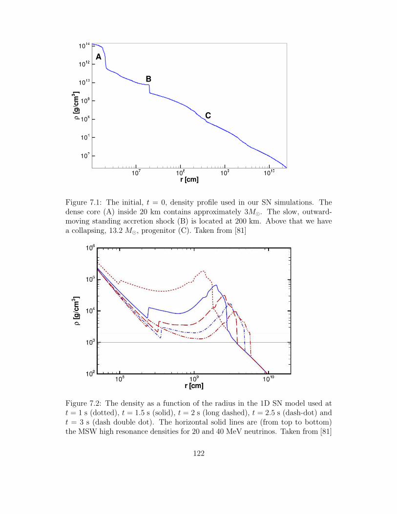
Figure 7.1: The initial, t = 0, density profile used in our SN simulations. Thedense core (A) inside 20 km contains approximately 3M⊙. The slow, outward-moving standing accretion shock (B) is located at 200 km. Above that we havea collapsing, 13.2 M⊙, progenitor (C). Taken from [81]
Figure 7.2: The density as a function of the radius in the 1D SN model used att = 1 s (dotted), t = 1.5 s (solid), t = 2 s (long dashed), t = 2.5 s (dash-dot) andt = 3 s (dash double dot). The horizontal solid lines are (from top to bottom)the MSW high resonance densities for 20 and 40 MeV neutrinos. Taken from [81]
122
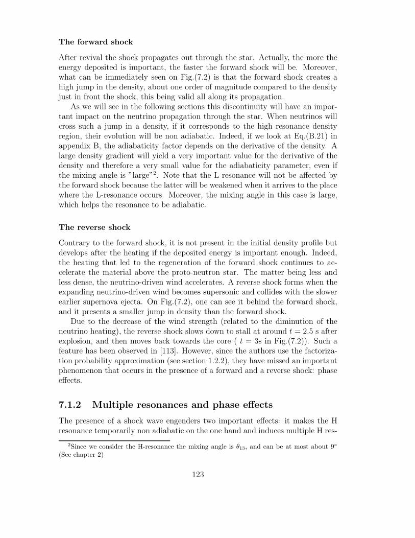
The forward shock
After revival the shock propagates out through the star. Actually, the more theenergy deposited is important, the faster the forward shock will be. Moreover,what can be immediately seen on Fig.(7.2) is that the forward shock creates ahigh jump in the density, about one order of magnitude compared to the densityjust in front the shock, this being valid all along its propagation.
As we will see in the following sections this discontinuity will have an impor-tant impact on the neutrino propagation through the star. When neutrinos willcross such a jump in a density, if it corresponds to the high resonance densityregion, their evolution will be non adiabatic. Indeed, if we look at Eq.(B.21) inappendix B, the adiabaticity factor depends on the derivative of the density. Alarge density gradient will yield a very important value for the derivative of thedensity and therefore a very small value for the adiabaticity parameter, even ifthe mixing angle is ”large”2. Note that the L resonance will not be affected bythe forward shock because the latter will be weakened when it arrives to the placewhere the L-resonance occurs. Moreover, the mixing angle in this case is large,which helps the resonance to be adiabatic.
The reverse shock
Contrary to the forward shock, it is not present in the initial density profile butdevelops after the heating if the deposited energy is important enough. Indeed,the heating that led to the regeneration of the forward shock continues to ac-celerate the material above the proto-neutron star. The matter being less andless dense, the neutrino-driven wind accelerates. A reverse shock forms when theexpanding neutrino-driven wind becomes supersonic and collides with the slowerearlier supernova ejecta. On Fig.(7.2), one can see it behind the forward shock,and it presents a smaller jump in density than the forward shock.
Due to the decrease of the wind strength (related to the diminution of theneutrino heating), the reverse shock slows down to stall at around t = 2.5 s afterexplosion, and then moves back towards the core ( t = 3s in Fig.(7.2)). Such afeature has been observed in [113]. However, since the authors use the factoriza-tion probability approximation (see section 1.2.2), they have missed an importantphenomenon that occurs in the presence of a forward and a reverse shock: phaseeffects.
7.1.2 Multiple resonances and phase effects
The presence of a shock wave engenders two important effects: it makes the Hresonance temporarily non adiabatic on the one hand and induces multiple H res-
2Since we consider the H-resonance the mixing angle is θ13, and can be at most about 9
(See chapter 2)
123
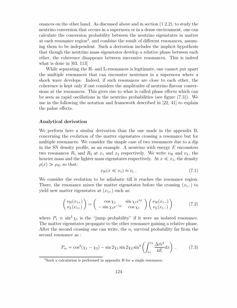
onances on the other hand. As discussed above and in section (1.2.2), to study theneutrino conversion that occurs in a supernova or in a dense environment, one cancalculate the conversion probability between the neutrino eigenstates in matterat each resonance region3, and combine the result of different resonances, assum-ing them to be independent. Such a derivation includes the implicit hypothesisthat though the neutrino mass eigenstates develop a relative phase between eachother, the coherence disappears between successive resonances. This is indeedwhat is done in [63, 113]
While separating the H- and L-resonances is legitimate, one cannot put apartthe multiple resonances that can encounter neutrinos in a supernova where ashock wave develops. Indeed, if such resonances are close to each other, thecoherence is kept only if one considers the amplitudes of neutrino flavour conver-sions at the resonances. This gives rise to what is called phase effects which canbe seen as rapid oscillations in the neutrino probabilities (see figure (7.3)). Weuse in the following the notation and framework described in [22, 41] to explainthe pahse effects.
Analytical derivation
We perform here a similar derivation than the one made in the appendix B,concerning the evolution of the matter eigenstates crossing a resonance but formultiple resonances. We consider the simple case of two resonances due to a dipin the SN density profile, as an example. A neutrino with energy E encounterstwo resonances R1 and R2 at x1 and x2 respectively. We write νH and νL, theheavier mass and the lighter mass eigenstates respectively. At x≪ x1, the densityρ(x)≫ ρR, so that:
νH(x≪ x1) ≈ νe . (7.1)
We consider the evolution to be adiabatic till it reaches the resonance region.There, the resonance mixes the matter eigenstates before the crossing (x1−) toyield new matter eigenstates at (x1+) such as:
(
νH(x1+)νL(x1+)
)
=
(
cosχ1 sinχ1eiϕ
− sinχ1e−iϕ cosχ1
)(
νH(x1−)νL(x1−)
)
. (7.2)
where P1 ≡ sin2 χ1 is the “jump probability” if it were an isolated resonance.The matter eigenstates propagate to the other resonance gaining a relative phase.After the second crossing one can write, the νe survival probability far from thesecond resonance as :
Pee = cos2(χ1 − χ2)− sin 2χ1 sin 2χ2 sin2
(∫ x2
x1
∆m2
4Edx
)
. (7.3)
3Such a calculation is performed in appendix B for a single resonance.
124
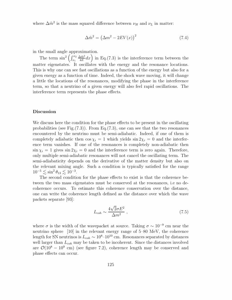
where ∆m2 is the mass squared difference between νH and νL in matter:
∆m2 =(
∆m2 − 2EV (x))2
(7.4)
in the small angle approximation.
The term sin2(
∫ x2
x1
∆m2
4Edx)
in Eq.(7.3) is the interference term between the
matter eigenstates. It oscillates with the energy and the resonance locations.This is why one can see fast oscillations as a function of the energy but also for agiven energy as a function of time. Indeed, the shock wave moving, it will changea little the locations of the resonances, modifying the phase in the interferenceterm, so that a neutrino of a given energy will also feel rapid oscillations. Theinterference term represents the phase effects.
Discussion
We discuss here the condition for the phase effects to be present in the oscillatingprobabilities (see Fig.(7.3)). From Eq.(7.3), one can see that the two resonancesencountered by the neutrino must be semi-adiabatic. Indeed, if one of them iscompletely adiabatic then cosχi = 1 which yields sin 2χi = 0 and the interfer-ence term vanishes. If one of the resonances is completely non-adiabatic thensinχi = 1 gives sin 2χi = 0 and the interference term is zero again. Therefore,only multiple semi-adiabatic resonances will not cancel the oscillating term. Thesemi-adiabaticity depends on the derivative of the matter density but also onthe relevant mixing angle. Such a condition is typically satisfied for the range10−5 . sin2 θ13 . 10−3.
The second condition for the phase effects to exist is that the coherence be-tween the two mass eigenstates must be conserved at the resonances, i.e no de-coherence occurs. To estimate this coherence conservation over the distance,one can write the coherence length defined as the distance over which the wavepackets separate [93]:
Lcoh ∼4√
2σE2
∆m2, (7.5)
where σ is the width of the wavepacket at source. Taking σ ∼ 10−9 cm near theneutrino sphere [10] in the relevant energy range of 5–80 MeV, the coherencelength for SN neutrinos is Lcoh ∼ 108–1010 cm. Resonances separated by distanceswell larger than Lcoh may be taken to be incoherent. Since the distances involvedare O(108 − 109 cm) (see figure 7.2), coherence length may be conserved andphase effects can occur.
125
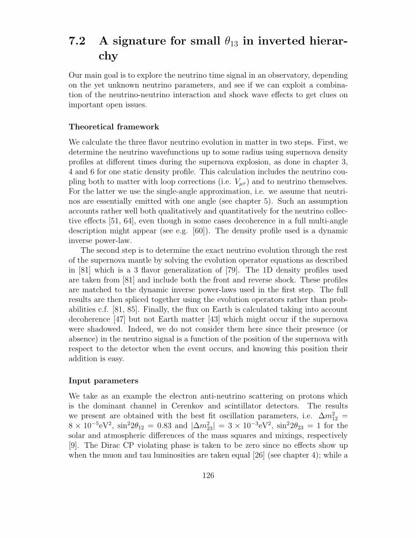
7.2 A signature for small θ13 in inverted hierar-
chy
Our main goal is to explore the neutrino time signal in an observatory, dependingon the yet unknown neutrino parameters, and see if we can exploit a combina-tion of the neutrino-neutrino interaction and shock wave effects to get clues onimportant open issues.
Theoretical framework
We calculate the three flavor neutrino evolution in matter in two steps. First, wedetermine the neutrino wavefunctions up to some radius using supernova densityprofiles at different times during the supernova explosion, as done in chapter 3,4 and 6 for one static density profile. This calculation includes the neutrino cou-pling both to matter with loop corrections (i.e. Vµτ ) and to neutrino themselves.For the latter we use the single-angle approximation, i.e. we assume that neutri-nos are essentially emitted with one angle (see chapter 5). Such an assumptionaccounts rather well both qualitatively and quantitatively for the neutrino collec-tive effects [51, 64], even though in some cases decoherence in a full multi-angledescription might appear (see e.g. [60]). The density profile used is a dynamicinverse power-law.
The second step is to determine the exact neutrino evolution through the restof the supernova mantle by solving the evolution operator equations as describedin [81] which is a 3 flavor generalization of [79]. The 1D density profiles usedare taken from [81] and include both the front and reverse shock. These profilesare matched to the dynamic inverse power-laws used in the first step. The fullresults are then spliced together using the evolution operators rather than prob-abilities c.f. [81, 85]. Finally, the flux on Earth is calculated taking into accountdecoherence [47] but not Earth matter [43] which might occur if the supernovawere shadowed. Indeed, we do not consider them here since their presence (orabsence) in the neutrino signal is a function of the position of the supernova withrespect to the detector when the event occurs, and knowing this position theiraddition is easy.
Input parameters
We take as an example the electron anti-neutrino scattering on protons whichis the dominant channel in Cerenkov and scintillator detectors. The resultswe present are obtained with the best fit oscillation parameters, i.e. ∆m2
12 =8 × 10⁻⁵eV2, sin22θ12 = 0.83 and |∆m2
23| = 3 × 10⁻³eV2, sin22θ23 = 1 for thesolar and atmospheric differences of the mass squares and mixings, respectively[9]. The Dirac CP violating phase is taken to be zero since no effects show upwhen the muon and tau luminosities are taken equal [26] (see chapter 4); while a
126
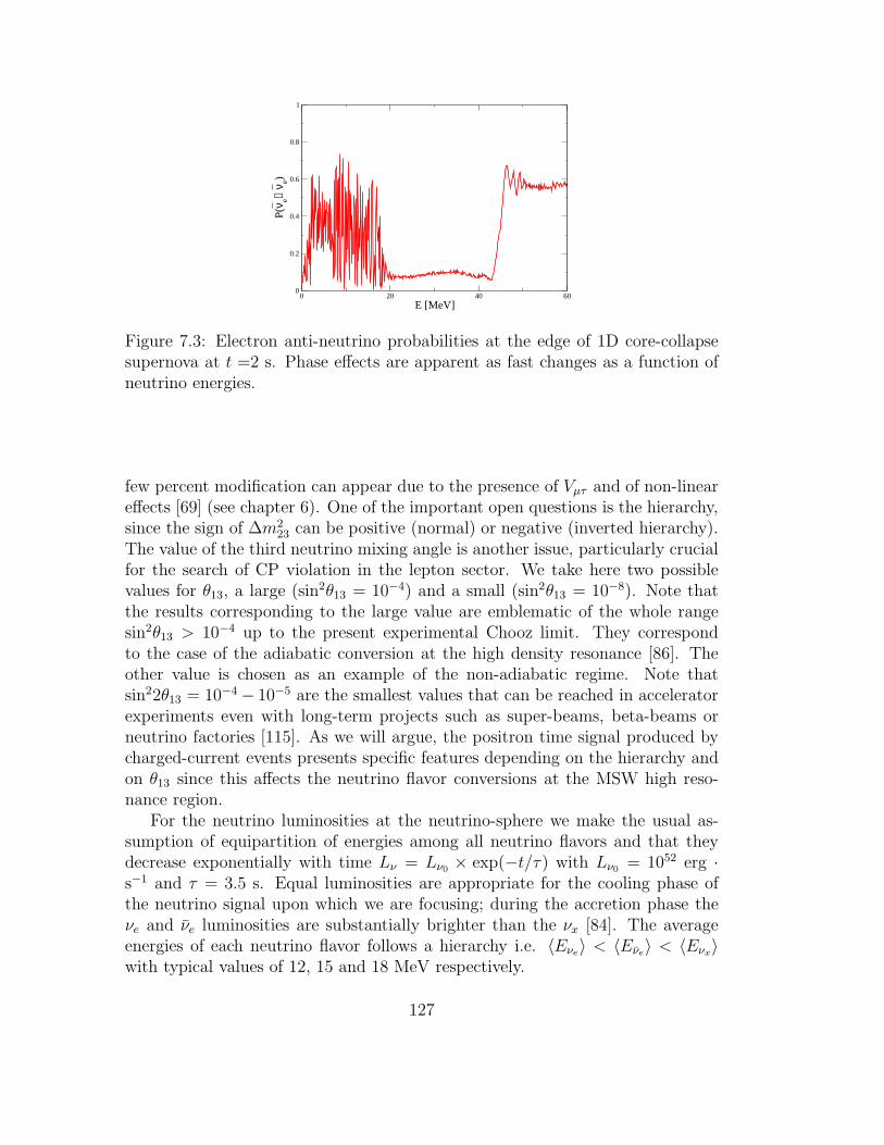
0 20 40 60E [MeV]
0
0.2
0.4
0.6
0.8
1
P(ν
e→ν e)
Figure 7.3: Electron anti-neutrino probabilities at the edge of 1D core-collapsesupernova at t =2 s. Phase effects are apparent as fast changes as a function ofneutrino energies.
few percent modification can appear due to the presence of Vµτ and of non-lineareffects [69] (see chapter 6). One of the important open questions is the hierarchy,since the sign of ∆m2
23 can be positive (normal) or negative (inverted hierarchy).The value of the third neutrino mixing angle is another issue, particularly crucialfor the search of CP violation in the lepton sector. We take here two possiblevalues for θ13, a large (sin2θ13 = 10−4) and a small (sin2θ13 = 10−8). Note thatthe results corresponding to the large value are emblematic of the whole rangesin2θ13 > 10−4 up to the present experimental Chooz limit. They correspondto the case of the adiabatic conversion at the high density resonance [86]. Theother value is chosen as an example of the non-adiabatic regime. Note thatsin22θ13 = 10−4− 10−5 are the smallest values that can be reached in acceleratorexperiments even with long-term projects such as super-beams, beta-beams orneutrino factories [115]. As we will argue, the positron time signal produced bycharged-current events presents specific features depending on the hierarchy andon θ13 since this affects the neutrino flavor conversions at the MSW high reso-nance region.
For the neutrino luminosities at the neutrino-sphere we make the usual as-sumption of equipartition of energies among all neutrino flavors and that theydecrease exponentially with time Lν = Lν0 × exp(−t/τ) with Lν0 = 1052 erg ·s−1 and τ = 3.5 s. Equal luminosities are appropriate for the cooling phase ofthe neutrino signal upon which we are focusing; during the accretion phase theνe and νe luminosities are substantially brighter than the νx [84]. The averageenergies of each neutrino flavor follows a hierarchy i.e. 〈Eνe
〉 < 〈Eνe〉 < 〈Eνx
〉with typical values of 12, 15 and 18 MeV respectively.
127
Phase effects
Figure (7.3) shows the electron anti-neutrino probability at the edge of the star,at a time when the shock wave has reached the region where MSW conversionmight occur. To comprehend such behaviour, one can see the different resonanceregions for the different energies. The multiple resonance interferences inducefast oscillations that show up as abrupt changes in the probabilities, below 20MeV. Indeed, looking at Fig.(7.2), the top horizontal solid line corresponds tothe resonance density for a 20 MeV neutrino. Therefore, all neutrinos with en-ergy below 20 MeV would have a similar horizontal line above the 20 MeV line.Those lines would cross the 2 s density profile in several points, so that suchneutrinos encounter multiple resonances. If these latter are semi-adiabatic, im-portant phases effects will appear as fast oscillations, this is what is observed onFig.(7.3). For energies above 45 MeV, an adiabatic conversion happened sinceat that time (t =2 s) the forward shock didn’t reach yet the MSW conversionfor those energies as can be seen on Fig. (7.2) with the lower horizontal solidline. The probability goes up to 0.6 and not 1 because with such oscillation pa-rameters the conversion is not complete. For energies between 20 and 45 MeV,the forward shock has reached the MSW conversion regions, as can be seen onFig.(7.2). Therefore such energies have undergone non adiabatic resonances, theelectron anti neutrino survival probability stays at a near zero value.
7.2.1 Signal on Earth
Let us now consider a supernova explosion located at 10 kpc from Earth.
The νe flux on Earth
In inverted hierarchy, for any value of θ13 (except zero), the electron (anti-)neutrino probability becomes very small in presence of ν − ν interaction (seechapter 5 Fig. 5.10). This implies that the corresponding fluxes have swappedwith the muon and tau neutrino fluxes and become “hot” at this point in theirpropagation. This differs from the previously standard paradigm, where the elec-tron anti-neutrinos enter the region of the MSW resonance with a “cold” spec-trum. As we will see this fact will imply a specific time signal in core-collapsesupernova observatories. A second swapping of the (anti)neutrino fluxes may oc-cur when they reach the MSW resonance region, depending on the adiabaticityof the resonance. One can see the consequences on the neutrino fluxes on Earthin Fig.(7.4).
At the early times (t . 1 s), for the inverted hierarchy and large θ13, anti-neutrinos undergo an adiabatic MSW resonance and have a “cold” spectrumon Earth4 (Figure 7.4). When the shock wave passes through the MSW high
4Note that the spectra mix slightly due to the θ12 rotation at the L resonance.
128
Figure 7.4: Electron anti-neutrino fluxes on Earth, in the case of adiabatic (“cold”spectrum, solid) and non-adiabatic (“hot” spectrum, dashed) conversions in thestar. t=1s
resonance region, important modifications of the neutrino fluxes occur. Thepresence of the shock wave renders the neutrino flavor conversion in this regionnon-adiabatic. Therefore the neutrino spectra on Earth remains “hot” (Figure7.4). Note that the adiabatic and non-adiabatic spectra will cross at some en-ergy, which in this case, is Eν = 20 MeV. These different regimes produce specificsignatures on the time signals, as we discuss now.
The positron signals in an observatory
We are considering the positron signal emitted from the inverse β reactions in thewater Cerenkov detector. The positron spectrum seen in a detector, Φe+(Ee+), isgiven by
Φe+(Ee+) = Np
∫
dEνeFνe
dσ
dEe+
(7.6)
where Np is the number of protons in the detector, Fνeis the electron antineutrino
flux on Earth and dσ/dEe+ is the differential cross section. Note that the positronspectrum is not the direct image of the νe flux and a certain correlation functionhas to be taken into account. More details concerning the positron spectrum can
129
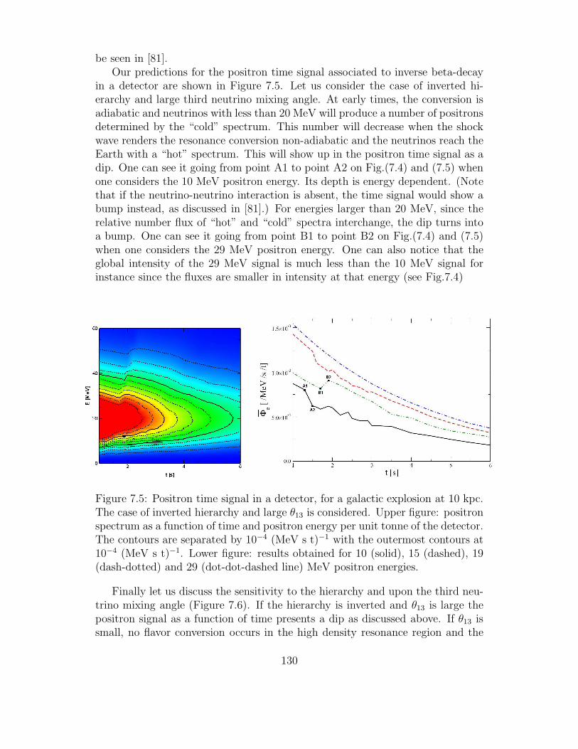
be seen in [81].Our predictions for the positron time signal associated to inverse beta-decay
in a detector are shown in Figure 7.5. Let us consider the case of inverted hi-erarchy and large third neutrino mixing angle. At early times, the conversion isadiabatic and neutrinos with less than 20 MeV will produce a number of positronsdetermined by the “cold” spectrum. This number will decrease when the shockwave renders the resonance conversion non-adiabatic and the neutrinos reach theEarth with a “hot” spectrum. This will show up in the positron time signal as adip. One can see it going from point A1 to point A2 on Fig.(7.4) and (7.5) whenone considers the 10 MeV positron energy. Its depth is energy dependent. (Notethat if the neutrino-neutrino interaction is absent, the time signal would show abump instead, as discussed in [81].) For energies larger than 20 MeV, since therelative number flux of “hot” and “cold” spectra interchange, the dip turns intoa bump. One can see it going from point B1 to point B2 on Fig.(7.4) and (7.5)when one considers the 29 MeV positron energy. One can also notice that theglobal intensity of the 29 MeV signal is much less than the 10 MeV signal forinstance since the fluxes are smaller in intensity at that energy (see Fig.7.4)
Figure 7.5: Positron time signal in a detector, for a galactic explosion at 10 kpc.The case of inverted hierarchy and large θ13 is considered. Upper figure: positronspectrum as a function of time and positron energy per unit tonne of the detector.The contours are separated by 10−4 (MeV s t)−1 with the outermost contours at10−4 (MeV s t)−1. Lower figure: results obtained for 10 (solid), 15 (dashed), 19(dash-dotted) and 29 (dot-dot-dashed line) MeV positron energies.
Finally let us discuss the sensitivity to the hierarchy and upon the third neu-trino mixing angle (Figure 7.6). If the hierarchy is inverted and θ13 is large thepositron signal as a function of time presents a dip as discussed above. If θ13 issmall, no flavor conversion occurs in the high density resonance region and the
130
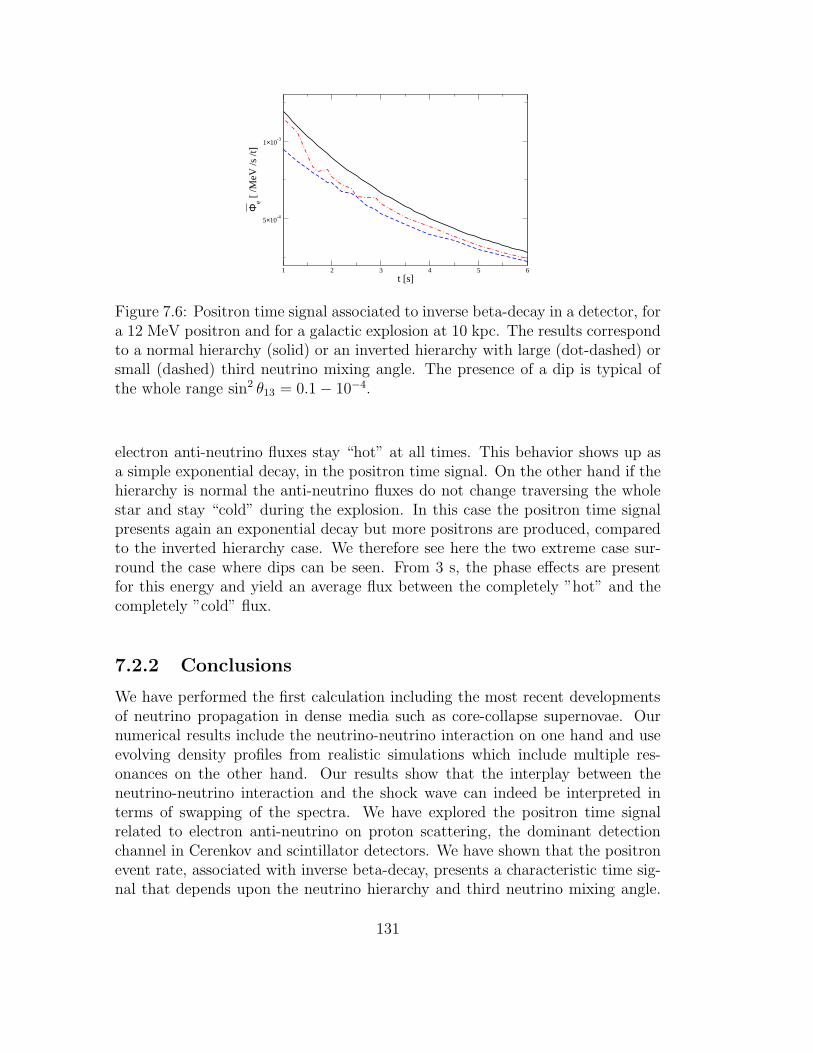
1 2 3 4 5 6t [s]
5×10⁻⁴
1×10⁻³
Φe [
/MeV
/s /t
]
Figure 7.6: Positron time signal associated to inverse beta-decay in a detector, fora 12 MeV positron and for a galactic explosion at 10 kpc. The results correspondto a normal hierarchy (solid) or an inverted hierarchy with large (dot-dashed) orsmall (dashed) third neutrino mixing angle. The presence of a dip is typical ofthe whole range sin2 θ13 = 0.1− 10−4.
electron anti-neutrino fluxes stay “hot” at all times. This behavior shows up asa simple exponential decay, in the positron time signal. On the other hand if thehierarchy is normal the anti-neutrino fluxes do not change traversing the wholestar and stay “cold” during the explosion. In this case the positron time signalpresents again an exponential decay but more positrons are produced, comparedto the inverted hierarchy case. We therefore see here the two extreme case sur-round the case where dips can be seen. From 3 s, the phase effects are presentfor this energy and yield an average flux between the completely ”hot” and thecompletely ”cold” flux.
7.2.2 Conclusions
We have performed the first calculation including the most recent developmentsof neutrino propagation in dense media such as core-collapse supernovae. Ournumerical results include the neutrino-neutrino interaction on one hand and useevolving density profiles from realistic simulations which include multiple res-onances on the other hand. Our results show that the interplay between theneutrino-neutrino interaction and the shock wave can indeed be interpreted interms of swapping of the spectra. We have explored the positron time signalrelated to electron anti-neutrino on proton scattering, the dominant detectionchannel in Cerenkov and scintillator detectors. We have shown that the positronevent rate, associated with inverse beta-decay, presents a characteristic time sig-nal that depends upon the neutrino hierarchy and third neutrino mixing angle.
131
For an inverted hierarchy and a large third neutrino mixing angle the event rateif found to decrease (increase) midway through the supernova neutrino signal forlow (high) neutrino energies. This general prediction agrees qualitatively withthe observed gap of low energy events in the supernova 1987A data [74, 31, 7]although, with so few observations, an emission model with no shock effects ismarginally compatible [83].
The signature relies upon: a) that the proto-neutron star is brighter in νe andνx at low energies, b) that the hierarchy is inverted so that collective effects swapthe νe than νx spectra prior to the H resonance, c) that neutrino propagationthrough the progenitor profile is adiabatic, d) the shock reaches the H resonanceswhile the supernova is still luminous. If, for example, the luminosities of νe andνx at low energy were comparable then there would little decrease in the positronevent rate midway through the signal but, on the flip side, a greater difference inluminosity exaggerates the event rate decrease. This signature might be robustin the presence of turbulence, although further investigation is required. Thereasoning is that the density profiles used here can be thought of as equivalent tothe ‘average’ profiles of Fogli et al. [65]. When these authors added turbulenceto the post shock region of their profiles they found that the size of the shockeffects were muted but, more importantly, they were not removed.
Finally the observation of the cross-over energy provides valuable informationabove the original neutrino fluxes. By measuring different positron energies in apossible future galactic core-collapse supernova explosion one might learn if thethird neutrino mixing angle is within (smaller) the window of achievability ofpresent (future) terrestrial experiments.
132
Part IV
Leptonic CP-violation in theearly Universe
133

Chapter 8
CP-violation effects on theneutrino degeneracy parameter
There are presently three observational evidences for the Big Bang Model: theuniversal expansion, the Cosmic Microwave Background Radiation (CMBR), andthe Big Bang Nucleosynthesis (BBN) (also called primordial nucleosynthesis).The latter evidence provides a probe of the Universe during its early evolution[107]. Indeed, it is during this epoch that the primordial abundances of lightnuclides (D, 3He, 4He, and 7Li) were produced. They are sensitive to the universaldensity of baryons and to the early Universe expansion rate, which at early timesis governed by the energy density of relativistic particles such as photons andneutrinos.
At a certain time, just before BBN, neutrinos decouple from matter and willconserve their thermal spectrum with a proper rescaling of the parameters due toredshift as the Universe will expand. Such relic neutrino background has neverbeen directly detected so we must resort to indirect means to infer its properties.One of the most useful tools available is naturally BBN [111]. By putting neutrinooscillations together with BBN, we may shed light on neutrino properties and/orcosmology. Our aim in this chapter is to investigate the influence of the CP-violating phase, contained in the MNSP matrix, on the value of the electronneutrino lepton asymmetry.
8.1 Introduction
8.1.1 The neutrino degeneracy parameter and implica-
tions
In the very early Universe, baryon-antibaryon pairs were as abundant as radi-ation. As the Universe expands and cools, the pairs annihilate, leaving behindany baryon excess established during the earlier evolution of the Universe. Subse-
135
quently, the number of baryons in a comoving volume of the Universe is preserved.After the e± pair annihilation, when the temperature drops below the electronmass, the number of CBR photons in a comoving volume is also preserved. It istherefore conventional to measure the universal baryon asymmetry by comparingthe number of (excess) baryons to the number of photons in a comoving volume(post e± annihilation). This ratio defines the baryon abundance parameter ηB:
ηB ≡nB − nB
nγ
= 6.14× 10⁻¹⁰(1.00± 0.04) (8.1)
The value of ηB comes from CMB anisotropies measured by WMAP [110].In addition with such asymmetry, BBN is sensitive to the expansion rate. For
the standard model of cosmology, the Friedman equation relates the expansionrate, quantified by the Hubble parameter H , to the matter-radiation content ofthe Universe:
H2 =8π
3GNρTOT (8.2)
where GN is Newton’s gravitational constant. During the epoch we are interestedin, roughly between 50 MeV and 1 MeV, the total energy density is dominated byradiation, i.e photons and ultra-relativistic particles, namely neutrinos, electronsand positrons. Contrary to the baryon asymmetry of the universe, the size of thelepton asymmetry is unknown. While some models predict a lepton asymmetrycomparable to the baryon asymmetry, it is also possible that such asymmetriesare disconnected and that the lepton asymmetry could be large enough to perturbthe standard BBN. Note that such large asymmetry would have to reside in theneutrino sector since neutrality ensures that the electron-positron asymmetryis comparable to the baryon asymmetry. In analogy with ηB which quantifiesthe baryon asymmetry, the neutrino asymmetry, Lν = Lνe
+ Lνµ+ Lντ
may bequantified by the neutrino chemical potentials µνα
(α ≡ e, µ, τ) or equivalentlythe degeneracy parameters ξνα
≡ µνα/Tν :
Lνα=nνα− nνα
nγ=
π2
12ζ(3)
(
Tνα
Tγ
)3(
ξα +ξ3α
π2
)
(8.3)
where ζ(3) ≃ 1.202. Prior to e± annihilation, Tν = Tγ, while post-e± annihilation(Tνα
/Tγ) = 4/11. In the rest of this chapter, since we consider neutrinos beforedecoupling, we will consider equal temperatures for neutrinos and photons.1 Sinceneutrinos and anti-neutrinos should be in chemical and thermal equilibrium untilthey decouple at temperature T ∼ 2 MeV, they may be well described by Fermi-Dirac distributions with equal and opposite chemical potentials:
f(p, ξ) =1
1 + exp(p/T + ξ)(8.4)
1Note that small differences in the temperature can come from out of equilibrium effects[88] During this epoch, neutrinos are slightly coupled when electron-positron pairs annihilatetransferring their entropy to photons. This process originates non-thermal distortions on theneutrino spectra which depend on neutrino flavour, larger for νe than for νµ or ντ .
136
where p denotes the neutrino momentum, T the temperature, and ξ the chemicalpotential in units of T . A nonzero chemical potential results in extra energydensity,
ρrad =
[
1 +7
8
(
4
11
)4/3
Neff
]
ργ (8.5)
such that the effective number of neutrinos is increased from the standard modelprescription by
∆Nν =30
7
(
ξ
π
)2
+15
7
(
ξ
π
)4
(8.6)
The effective number of neutrino families Neff parametrizes the cosmic radiationafter e+e− annihilation. The standard value for Neff is 3.046, it deviates from3 because of residual neutrino heating. Actually, large chemical potentials affectBBN in two ways:
1. The extra energy density increases the expansion rate of the universe, thusincreasing the BBN helium abundance, and also alters CMB results. This setsweak bound | ξα |. 3, for all three flavours.
2. An additional, much stronger limit can be placed on the νe − νe asymme-try, as it directly affects the neutron to proton ratio prior to BBN by alteringbeta-equilibrium (n+ νe ↔ p+ e− and p + νe ↔ n+ e+). For example, positiveξe increases the νe abundance relative to νe, thus lowering the neutron to protonratio and decreasing the helium yield. This sets the limit | ξe |. 0.04. However,it is possible that the two effects compensate for each other, i.e. the effects of asmall ξe are partially undone by an increased expansion rate due to a large ξµ,τ .In this case the bounds become [82, 73]:
−0.01 < ξe < 0.22 (8.7)
| ξµτ |< 2.6 (8.8)
We now know that neutrinos oscillate, each individual lepton number Le, Lµ
and Lτ is violated and only the total lepton number is conserved. Since the mix-ing angle are large enough, they can lead to equilibration of all flavours beforeBBN. Therefore, if a large asymmetry is hidden in ξµ,τ it will transferred to ξe wellbefore freeze-out at T ≃ 1 MeV. Consequently, in such situation, the stringentlimit of BBN on ξe would apply to all flavours improving the bound on ξµ,τ [48].
8.1.2 The neutron to proton ratio
The neutron-to-proton ratio is set by the competition of the expansion rate ofthe universe and the rates of the following lepton capture/decay processes:
νe + n p+ e−, (8.9)
137
νe + p n+ e+, (8.10)
n p+ e− + νe. (8.11)
We denote the forward and reverse rates of the first process as λνen and λe−p,respectively. Likewise, the forward and reverse rates of the second process areλνep and λe+n, respectively, while those of the third process are λn decay and λpeνe
,respectively. At high enough temperature (T ≫ 1 MeV), where these rates arevery fast, the isospin of any nucleon will flip from neutron to proton and back at arate which is rapid compared to the expansion rate of the universe, establishing asteady state equilibrium. As the universe expands and the temperature drops therates of the lepton capture processes will drop off quickly. Eventually the leptoncapture rates will fall below the expansion rate and n/p will be frozen in (exceptfor free neutron decay). However, there is no sharp freeze-out, the neutron-to-proton ratio n/p is modified by the lepton capture reactions down to temperaturesof several hundred keV and by neutron decay through the epoch of alpha particleformation Tα. The evolution of the electron fraction Ye = 1/(1+n/p) throughoutthe expansion is governed by
dYe
dt= Λn − Ye (Λn + λνep + λe−p + λpeνe
) (8.12)
where we took into account the rates of the neutron destroying processes Λn =λνen + λe+n + λndecay and the weak isospin changing rates. In the limit where theisospin flip rate is fast compared to the expansion rate H , the neutron-to-protonratio has a steady state equilibrium value (dYe/dt = 0) given by [99]:
n
p=
λνep + λe−p + λpeνe
λνen + λe+n + λn decay, (8.13)
≈ λνep + λe−p
λνen + λe+n
.
If the electron neutrinos and antineutrinos and the electrons and positrons allhave Fermi-Dirac energy spectra, then Eq.(8.13) can be reduced to2 [37]
n
p≈ (λe−p/λe+n) + e−ξe+ηe−δmnp/T
(λe−p/λe+n) eξe−ηe+δmnp/T + 1, (8.14)
where ηe = µe/T is the electron degeneracy parameter and (mn −mp) /T ≡δmnp/T ≈ 1.293 MeV/T is the neutron-proton mass difference divided by tem-perature. If chemical equilibrium is achieved, then we have µe − µνe
= µn − µp,where µn and µp are the neutron and proton total chemical potentials, respec-tively, and in this case Eq.(8.14) reduces to
n
p≈ e(µe−µνe−δmnp)/T . (8.15)
2We assume here identical neutrino and plasma temperatures and neglect the neutrondecay/three-body capture processes of Eq.(8.11) as done in [1].
138
From Eq.(8.15), we can conclude, for example, that a positive chemical potentialfor electron neutrinos (i.e. an excess of νe over νe) would imply a decrease in theneutron abundance which translates, in turn, into a decrease in the predicted 4Heyield since in mass fraction, we have:
Xα ≈2 (n/p)
(n/p+ 1). (8.16)
Indeed, in the early Universe, alpha particles win the competition between en-tropy and binding energy because the entropy per baryon is very high and al-pha particles have a binding per nucleon not very different from iron. At atemperature Tα ∼ 100 keV, alpha particles form rapidly, incorporating almostall neutrons. Therefore, the primordial 4He yield is determined roughly by theneutron-to-proton ratio n/p at Tα. The standard BBN 4He mass fraction yieldprediction is (24.85± 0.05)% using the CMB anisotropy-determined baryon den-sity [40].
The idea we wish to explore is if distortions in the νe and νe energy spectrastemming from the CP-violating phase can alter lepton capture rates on nucleonsand thereby change n/p and the 4He yield.
8.2 Neutrino flavor oscillations in the early uni-
verse
We study the effect of three-neutrino flavour oscillations on the process of neu-trino decoupling by solving the momentum-dependent kinetic equations for theneutrino spectra. We also include the muon-antimuon interactions annihilationwhose presence is not negligible for our purpose: to study the effects of the CP-violating phase on ξe and consequently on the neutron to proton ratio.
8.2.1 Theoretical framework
In order to study neutrino oscillations in the early universe we characterize theneutrino ensemble in the usual way by generalized occupation numbers, i.e. by 3× 3 matrices as described in appendix B. The form of the density matrices for amode with momentum p is
ρν(p, t) ≡
ρνeeρνeµ
ρνeτ
ρνµeρνµµ
ρνµτ
ρντeρντµ
ρνττ
(8.17)
Initially, the density matrix can be written as :
ρν(p, t = 0) ≡
f(p, ξe) 0 00 f(p, ξµ) 00 0 f(p, ξτ)
(8.18)
139
Indeed, initially we consider a time where the temperature is between 100 MeVand 10 MeV, and neutrinos are in thermal and chemical equilibrium. The equa-tions of motion for the density matrices in an expanding universe are :
i(∂t−Hp∂p)ρ(p, t) =
[(
UM2U †
2p− 8√
2GFp
3m2W
E
)
+√
2GF (ρ− ρ), ρ(p, t)]
+C[ρ(p, t)],
(8.19)where H = a(t)/a(t) is the Hubble parameter (a(t) the expansion parameter),GF is the Fermi constant and mW the W boson mass. On the l.h.s. of Eq.(8.19),we substituted ∂t → ∂t −Hp∂p with H the cosmic expansion parameter becausethe Universe is expanding.
The vacuum term
The first term in the commutator [·, ·] UM2U†
2pis the vacuum oscillation term where
M2 = diag(m21, m
22, m
23) and U the unitary Maki-Nakagawa-Sakata-Pontecorvo
matrix as described in appendix A.
The matter term
The second term in the commutator
−8√
2GFp
3m2W
E ≡ −8√
2GFp
3m2W
(〈Eℓ−〉nℓ− + 〈Eℓ+〉nℓ+) (8.20)
represents the energy densities of charged leptons and corresponds to the refrac-tive effects of the medium that neutrinos experience. Actually, this term is dueto the presence of thermally populated charged leptons in the plasma, which in-duces a thermal potential from finite-temperature modification of the neutrinomass [108, 91]. E is the 3× 3 flavor matrix of charged-lepton energy densities:
E =
Eee + Eµµ 0 00 Eµµ 00 0 0
. (8.21)
where
Eαα =gα
2π2
∫ ∞
0
dpp2 E
1 + exp ET
(8.22)
with E =√
p2 +mµ±2 and gα is the number of spin states of the species, for
electrons for instance ge = 2×2 = 4, since the spin can be +12
or −12
and we haveto count the particle and its anti-particle, here the positron. For electrons andpositrons, since T, p >> me± we consider that those particles are ultra-relativisticthen E ≃ p. Therefore, we have:
Eee =2T 4
π2
∫ ∞
0
duu3
1 + exp u= −2T 4
π2Li4(−1)Γ(4) (8.23)
140
and we finally obtain3:
Eee =7π2
60T 4. (8.24)
For muons and anti-muons, since T, p << mµ± , if we consider that thoseparticles are non relativistic then
E ≃ mµ± +p2
2mµ±
. (8.25)
Therefore we finally obtain4:
Eµµ ≃2
π2mµ±(2mµ±T )
32 exp(
−mµ±
T)
∫ ∞
0
u2du exp(−u2)
≃√
2m52µ
π32
exp(−mµ
T) (8.26)
Note that the background potential arising, due to asymmetries in charged lep-tons, is nonzero for electron and muon neutrinos, to maintain charge neutralityof the baryon contaminated plasma. Due to the smallness of the baryon asym-metry relative to number densities of thermalized species, these terms are alwaysnegligible in comparison with the other terms in the Hamiltonian [2].
The neutrino-neutrino interaction
The third term in the commutator√
2GF (ρ − ρ) represents the neutrino self-interactions and is responsible for synchronizing the neutrino ensemble, as seenin chapter 5.
The collision term
Finally, the term C[ρ(p, t)] describes the collisions of neutrinos with e±, µ± oramong themselves and is proportional to G2
F . In order to properly calculatethe neutrino heating process, one should consider the exact collision integralIνα
[49, 50, 88] that includes all relevant two-body weak reactions of the typeνα(1) + 2 −→ 3 + 4 involving neutrinos ,e± and µ±,
Iνα
[
fνe, fνµ
, fντ
]
= 12 E1
∑
reactions
∫
d3p2
2 E2 (2 π)3d3p3
2 E3 (2 π)3d3p4
2 E4 (2 π)3
×(2 π)4 δ(4) (p1 + p2 − p3 − p4) F [αα(p1), f2, f3, f4] |M12→34|2 ,
Here F ≡ f3f4 (1− αα(p1)) (1− f2) − αα(p1)f2 (1− f3) (1− f4) is the statis-tical factor (when the particle i = 2, 3, 4 is a neutrino νβ one substitutes fi
3Using the relation Li4(−1) + Li4(1) = Li4(1)8 , which means −Li4(−1) = 7
8Li4(1) = 78ζ(4).
4Since∫∞0
duu2 exp(−u2) =√
π
4 .
141
with the corresponding diagonal term ββ(pi)), and M12→34 is the process ampli-tude. We approximate collisions with a simple damping prescription of the formC[ραβ(p, t)] = −Dpραβ(p, t) . These damping factors for the off-diagonal elementsof ρ(p, t) in the weak interaction basis, mimicks the destruction of phase coher-ence by flavor-sensitive collisions. Here we have decided to use the simplifiedassumption following [48]. To sum up about the evolution equation, the diag-onal elements change by collisions and by oscillations, whereas the off-diagonalelements change by oscillations and damping. Finally we can write
C[ρ(p, t)] ≡
iDe−µ,τ (f(p, ξe)− ρνeνe) −iDe−µ,τρνeνµ
−iDe−µ,τρνeντ
−iDe−µ,τρνµνeiDe−µ,τ (f(p, ξµ)− ρνµνµ
) −iDµτρνµντ
−iDe−µ,τρντ νe−iDµ−τρντ νµ
iDe−µ,τ (f(p, ξτ)− ρντ ντ)
(8.27)
with De−µ,τ = 2× (4sin4θW − 2sin2θW + 2)F0 and Dµ−τ = 2× (2sin4θW + 6)F0
[48].
8.2.2 The comoving variables
It is more convenient since the universe is expanding to use comoving variable.We therefore define the dimensionless expansion rate by:
x ≡ mR , y ≡ pR , (8.28)
where R is the universe scale factor and m an arbitrary mass scale that we chooseto be 1 MeV. With such new variable we rewrite Eq.(8.19). We first consider thel.h.s. of Eq.(8.19) by expressing the differential of ρ(x, y) over dt:
dρ(t, p)
dt=
(
∂ρ
∂x
)
y
dx
dt+
(
∂ρ
∂y
)
x
dy
dt
= mR
(
∂ρ
∂x
)
y
+mR
(
∂ρ
∂y
)
x
= Hx
(
∂ρ
∂x
)
y
+ pH
(
∂ρ
∂p
)
x
(8.29)
which finally yields :(
∂ρ
∂t− pH ∂ρ
∂p
)
= Hx∂ρ
∂x(8.30)
Consequently, the equation of motion for the period of expansion we are interestedin, is:
iHx(∂x)ρ(x, y) =
[(
UM2U †
2y− 8√
2GF y
3m2W
E
)
+√
2GF (ρ− ρ), ρ(x, y)]
+C[ρ(x, y)],
(8.31)
142
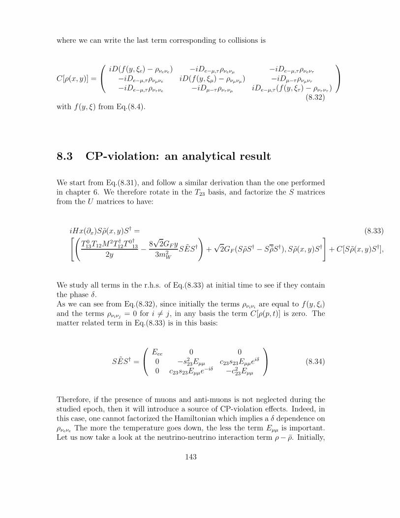
where we can write the last term corresponding to collisions is
C[ρ(x, y)] =
iD(f(y, ξe)− ρνeνe) −iDe−µ,τρνeνµ
−iDe−µ,τρνeντ
−iDe−µ,τρνµνeiD(f(y, ξµ)− ρνµνµ
) −iDµ−τρνµντ
−iDe−µ,τρντ νe−iDµ−τρντ νµ
iDe−µ,τ (f(y, ξτ)− ρντ ντ)
(8.32)with f(y, ξ) from Eq.(8.4).
8.3 CP-violation: an analytical result
We start from Eq.(8.31), and follow a similar derivation than the one performedin chapter 6. We therefore rotate in the T23 basis, and factorize the S matricesfrom the U matrices to have:
iHx(∂x)Sρ(x, y)S† = (8.33)
[(
T 013T12M
2T †12T
0†13
2y− 8√
2GF y
3m2W
SES†
)
+√
2GF (SρS† − SρS†), Sρ(x, y)S†
]
+ C[Sρ(x, y)S†],
We study all terms in the r.h.s. of Eq.(8.33) at initial time to see if they containthe phase δ.As we can see from Eq.(8.32), since initially the terms ρνiνi
are equal to f(y, ξi)and the terms ρνiνj
= 0 for i 6= j, in any basis the term C[ρ(p, t)] is zero. Thematter related term in Eq.(8.33) is in this basis:
SES† =
Eee 0 00 −s2
23Eµµ c23s23Eµµeiδ
0 c23s23Eµµe−iδ −c223Eµµ
(8.34)
Therefore, if the presence of muons and anti-muons is not neglected during thestudied epoch, then it will introduce a source of CP-violation effects. Indeed, inthis case, one cannot factorized the Hamiltonian which implies a δ dependence onρνeνe
The more the temperature goes down, the less the term Eµµ is important.Let us now take a look at the neutrino-neutrino interaction term ρ− ρ. Initially,
143
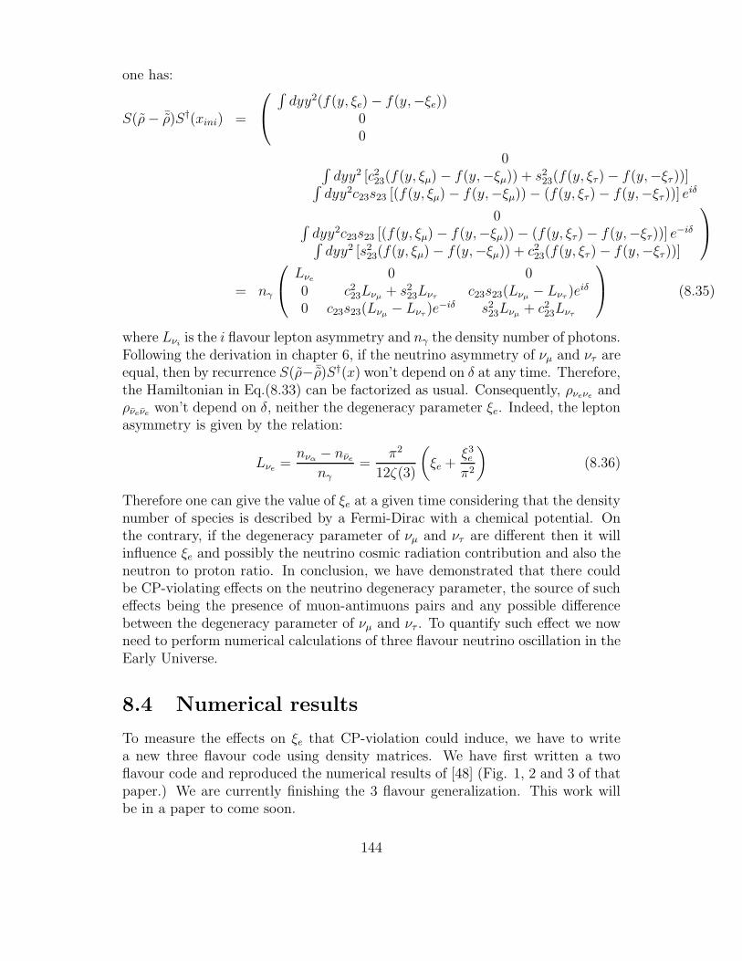
one has:
S(ρ− ¯ρ)S†(xini) =
∫
dyy2(f(y, ξe)− f(y,−ξe))00
0∫
dyy2 [c223(f(y, ξµ)− f(y,−ξµ)) + s223(f(y, ξτ)− f(y,−ξτ))]
∫
dyy2c23s23 [(f(y, ξµ)− f(y,−ξµ))− (f(y, ξτ)− f(y,−ξτ))] eiδ
0∫
dyy2c23s23 [(f(y, ξµ)− f(y,−ξµ))− (f(y, ξτ)− f(y,−ξτ))] e−iδ∫
dyy2 [s223(f(y, ξµ)− f(y,−ξµ)) + c223(f(y, ξτ)− f(y,−ξτ))]
= nγ
Lνe0 0
0 c223Lνµ+ s2
23Lντc23s23(Lνµ
− Lντ)eiδ
0 c23s23(Lνµ− Lντ
)e−iδ s223Lνµ
+ c223Lντ
(8.35)
where Lνiis the i flavour lepton asymmetry and nγ the density number of photons.
Following the derivation in chapter 6, if the neutrino asymmetry of νµ and ντ areequal, then by recurrence S(ρ− ¯ρ)S†(x) won’t depend on δ at any time. Therefore,the Hamiltonian in Eq.(8.33) can be factorized as usual. Consequently, ρνeνe
andρνeνe
won’t depend on δ, neither the degeneracy parameter ξe. Indeed, the leptonasymmetry is given by the relation:
Lνe=nνα− nνe
nγ=
π2
12ζ(3)
(
ξe +ξ3e
π2
)
(8.36)
Therefore one can give the value of ξe at a given time considering that the densitynumber of species is described by a Fermi-Dirac with a chemical potential. Onthe contrary, if the degeneracy parameter of νµ and ντ are different then it willinfluence ξe and possibly the neutrino cosmic radiation contribution and also theneutron to proton ratio. In conclusion, we have demonstrated that there couldbe CP-violating effects on the neutrino degeneracy parameter, the source of sucheffects being the presence of muon-antimuons pairs and any possible differencebetween the degeneracy parameter of νµ and ντ . To quantify such effect we nowneed to perform numerical calculations of three flavour neutrino oscillation in theEarly Universe.
8.4 Numerical results
To measure the effects on ξe that CP-violation could induce, we have to writea new three flavour code using density matrices. We have first written a twoflavour code and reproduced the numerical results of [48] (Fig. 1, 2 and 3 of thatpaper.) We are currently finishing the 3 flavour generalization. This work willbe in a paper to come soon.
144
Part V
Conclusion
145

In this thesis, we have studied several unknown neutrino properties in theastrophysical and also cosmological contexts.
The two first works have focussed on the study of possible effects coming fromthe CP-violating Dirac phase δ in the supernova environment. Many questionsremain concerning supernova physics such as the the precise mechanism of theexplosion and the nucleosynthesis of heavy elements (r-process). Neutrinos maybring some answers, since electron (anti-) neutrinos interact with matter and in-fluence the supernova observables like the electron fraction. Therefore, besidesgetting information on this crucial open question, the study of the influence ofthe unknown CP-violating phase on the neutrino fluxes and on the electron frac-tion could bring a new understanding of these open issues. Investigating such apossibility, we have first derived an analytic formula proving that no CP-violatingeffects could be present in the electron (anti-) neutrino flux and a fortiori in theelectron fraction, if and only if the flux of νµ is equal to the flux of ντ at the neu-trinosphere. Our demonstration is exact and valid for any matter density profile.This result validates all the litterature that uses the latter hypothesis while notconsidering the leptonic CP-violating phase. By relaxing this assumption, thanksto a code that we have developped, we have obtained that small effects can come–from a non-zero δ– on the νe (νe) flux and on the electron fraction. We havealso numerically calculated the effects of this Dirac phase on the number of eventsproduced by electron anti-neutrinos via inverse beta reactions in an observatoryon Earth.
Actually, the first picture of neutrino interacting with matter inside the su-pernova that we have based our calculation upon, was incomplete. First, onehas to take into account the one-loop corrections with matter. We have showedthat such a term differentiates νµ from ντ and induces a δ dependence on theelectron (anti-) neutrino survival probability, and consequently on the electron(anti-) neutrino flux.
In addition to such a correction, a new paradigm in neutrino physics hassettled during the last few years: neutrino-neutrino interactions must be takeninto account. Using a different approach, to analytically study the influence ofthe ν − ν interaction when δ is non zero, we have demonstrated that only whentaking different νµ and ντ fluxes, a δ dependence can arise from this term, in asimilar way as when one-loop corrections are considered. On the other hand, anew phenomenology is associated to such non-linear interactions that we haveincluded in our previous code. Reproducing the different collective behavioursthat emerge, we have studied the consequences of this new interaction on the νe
and νe fluxes inside the supernova, taking a non zero δ. It turns out that thenon-linearity amplifies the effects of δ present, due to the one-loop corrections,to a possible 10% effect in the supernova.
In the same time than the development of numerically demanding neutrino-neutrino interaction codes, people have also been interested in an important en-hancement of supernova models used in neutrino astrophysics, the use of a dy-
147
namic density profile with shock waves. Indeed, such dynamic profiles can leadto forward and reverse shock responsible for new neutrino features such as phaseeffects or non-adiabatic high resonances. The aim of the third work has been toobtain a state of the art neutrino flux calculation, the first one including boththe neutrino-neutrino interaction and a dynamic density profile with forward andreverse shocks. Such a code calculates the neutrino propagation through the su-pernova using wave functions ensuring that all relevant phase effects have beentaken into account. Consequently, we have been able to predict, in the invertedhierarchy case, the number of positron events, associated to inverse β decay, froma galactic supernova explosion in a very realistic way. We have shown that a dip,consequence of the shock wave and of the self-interactions, should be seen in thepositron signal from about 2 seconds after the bounce, during a few seconds, fora certain range of positron energies. Such a result looks particularly promisingalso in view of future large scale supernova neutrino observatories currently understudy.
Finally, as an application to our previous findings on δ effects, we have in-vestigated the possible consequences of the CP-violating phase before neutrinodecoupling in the Early Universe. The possible observables are the electron neu-trino degeneracy parameter and consequently the neutron to proton ratio whichplays a crucial role in BBN. Following a similar derivation obtained in the super-nova context, we have been able to show under which conditions the CP-violatingphase should have an impact on ξe. Indeed, if one takes into account the muonanti-muon pair interaction with neutrinos then, as for the one loop correctionsin the supernova context, no factorization of δ out of the Hamiltonian is possi-ble. Moreover, if we consider different initial degeneracy parameters for νµ andντ , then we will also see δ effects on ξe. We are currently finishing to write a 3flavour code using density matrices to quantify the effects induced by δ in suchcosmological environment.
The results of this PhD thesis, mainly turned on the effects of the CP-violatingphase on the neutrino fluxes in dense matter, have allowed us to clearly identifyunder which conditions there can be CP violation effects in the astrophysical(core-collapse supernovae) and also in the cosmological (before BBN) contexts.Our results have numerous implications and applications. From the point of viewof neutrino propagation, several improvements can be made. For example, oneshould perform demanding numerical calculations of the CP effects in the super-nova environment with three-dimensional multi-angle and dynamic treatment ofthe neutrino fluxes, including eventually turbulence effects. Besides, to come to adefinite statement concerning possible effects on the r-process much further workis still needed. With the obtained hindsight on this subject, one can think of di-rect applications of the analytic derivations and in particular, calculate preciselywhat could be the difference between the νµ and ντ fluxes at the neutrinosphere.Such differences could not only come from one loop corrections but also fromBeyond Standard Model physics like Flavour Changing Neutral Current for in-
148
stance. Future discoveries, e.g. from LHC, could therefore imply effects in thesupernova and cosmological (before BBN) contexts through CP-violation in thelepton sector. Let us hope that the new paths opened will lead to interestingdiscoveries and may be the key to some crucial problems related to astrophysicaland cosmological neutrinos.
149

150
Part VI
Appendix
151

Appendix A
The MNSP matrix and itsparametrization
In the standard model CP-violation is limited to the hadronic sector. Since theexperimental evidence that neutrinos oscillate (meaning they are massive) thestandard model has to be extended and a mixing matrix for leptons introduced.Since leptons constitutes a family of three particles (of non-degenerate masses),CP-violation becomes possible in the leptonic sector. In the standard model,neutrinos are the only elementary fermions with zero charge. This unique statusimplies that neutrinos can be of two different types, namely either Dirac or Ma-jorana particles. Double beta decay experiments can discriminate the nature ofneutrino. Let us first focus on the case where neutrinos are Dirac particles. Atthe end of this appendix we will comment on the Majorana case.
A.1 The Dirac neutrino case
If neutrinos are Dirac particles they are the same as the other fermions andneutrinos with right helicity must exist. The right and left handed spinors aremixed via a mass matrix, and the Dirac mass term for neutrinos is:
−LD = νfiL(mD)ij ν
fjR + h.c. (A.1)
Here the superscript f is used to denote the flavour eigenstate fields. Therefore,the part of the Lagrangian that describes the lepton masses and charged currentinteractions is
−LW+m+D =g√2lf
iL γµ νf
iLW−µ + l
f
iL(ml)ijlfjR + νf
iL(mD)ij νfjR + h.c. (A.2)
where the li can be e, µ, τ . This expression shows that neutrino oscillations, dueto the presence of the Dirac neutrino mass term, violate individual lepton flavournumber Le, Lµ and Lτ while the total lepton number L = Le + Lµ + Lτ is still
153
conserved. Considering the most general case where the mass matrix of chargedleptons ml and the neutrino mass matrix mD are complex matrices, we can usebi-unitary transformations to diagonalize them.Let us write
lfL = VL lmL , lfR = VR l
mR νf
L = UL νmL , νf
R = UR νmR , (A.3)
and choose the unitary matrices VL, VR, UL and UR so that they diagonalize themass matrices of charged leptons and neutrinos:
V †L ml VR = (ml)diag = diag(me, mµ, mτ ) (A.4)
U †LmD UR = (mD)diag = diag(mν1, mν2, mν3).
The fields lmiL, lmiR, νmiL and νm
iR with the superscripts m are then the componentsof the Dirac mass eigenstate fields em
i = emiL + em
iR and νmi = νm
iL + νmiR. The
Lagrangian in eq. (A.2) can be written in the mass eigenstate basis as
−LW+m+D =g√2ei
m γµ (V †LUL)ij ν
mLj W
−µ +mlie
mLie
mRi +mDi ν
mLiν
mRi + h.c. , (A.5)
where mli are the charged lepton masses, namely me, mµ and mτ . and mDi are
the neutrino masses. The matrix U = V †LUL is called the lepton mixing matrix,
or Maki-Nakagawa-Sakata-Pontecorvo (MNSP) matrix [? ]. It is the leptonicanalog of the CKM mixing matrix. It relates a neutrino flavour eigenstate |νf
a 〉produced or absorbed alongside the corresponding charged lepton, to the masseigenstates |νm
i 〉:|νf
a 〉 = U∗ai |νm
i 〉 , (A.6)
A.2 The parametrization of the MNSP matrix
In general a unitary N ×N matrix depends on N2 independent real parametersthat can be divided into: = N(N − 1)/2 mixing angles and N(N + 1)/2 phases.Hence the leptonic mixing matrix with N = 3 can be written in terms of threemixing angle and six phases.In the Dirac case, 2N − 1 phases can be removed by a proper rephasing ofthe left handed fields: the lepton mass terms νRνL + h.c. remains unchangedsince the phases can be absorbed into the corresponding rephasing of the right-handed fields. Only N(N + 1)/2− (2N − 1) = (N − 1)(N − 2)/2 physical phasesremain. Thus, in the Dirac case CP violation is only possible in the case ofN ≥ 3 generations. Since we have three generations, the MNSP matrix is madeof 3(3 − 1)/2 = 3 mixing angles and (3 − 1)(3 − 2)/2 = 1 physical phase. Thisphysical phase is the CP-violating phase. The neutrino flavour eigenstate andmass eigenstate fields are related through
νeL
νµL
ντL
= UMNSP
ν1L
ν2L
ν3L
=
Ue1 Ue2 Ue3
Uµ1 Uµ2 Uµ3
Uτ1 Uτ2 Uτ3
ν1L
ν2L
ν3L
. (A.7)
154
This matrix is a (complex) unitary matrix, therefore we have:
det(U) = eiΦ (A.8)
= Ue1(Uµ2Uτ3 − Uτ2Uµ3)− Uµ1(Ue2Uτ3 − Uτ2Uµ3) + Uτ1(Ue2Uµ3 − Uµ2Ue3)
We choose to express Uµ1, Uτ1, Uµ2, Uτ2 as a function of the other terms of theU matrix. To do so, we multiply the relation (A.8) by each of those terms, takethe conjugate of the equation and use the unitarity conditions. Let us make anexample with Uµ1. From Eq.(A.8), we obtain
e−iΦU∗µ1 = U∗
µ1(det(U))∗
= U∗µ1Ue1(Uµ2Uτ3 − Uτ2Uµ3)
− | Uµ1 |2 (Ue2Uτ3 − Uτ2Uµ3)
+ U∗µ1Uτ1(Ue2Uµ3 − Uµ2Ue3) (A.9)
Knowing that
U∗µ1Ue1 = −Ue2U
∗µ2 − Ue3U
∗µ3 (A.10)
and
U∗µ1Uτ1 = −Uτ2U
∗µ2 − Uτ3U
∗µ3 (A.11)
we have :Uµ1 = eiΦ (Uτ2Ue3 − Ue2Uτ3)
∗ (A.12)
With similar derivations, we obtain for Uτ1, Uµ2, Uτ2
Uτ1 = eiΦ (Ue2Uµ3 − Uµ2Ue3)∗
Uµ2 = eiΦ (Ue1Uτ3 − Uτ1Ue3)∗
Uτ2 = eiΦ (Uµ1Ue3 − Ue1Uµ3)∗ (A.13)
For the remaining terms we have the following two relations due to the unitarity:
| Ue1 |2 + | Ue2 |2 + | Ue3 |2= 1 (A.14)
and| Uτ3 |2 + | Uµ3 |2 + | Ue3 |2= 1. (A.15)
These relations are the same as those for spherical coordinates in a 3D Euclidianspace. We choose:
Ue1 = eiφe1 cosα cosβ
Ue2 = eiφe2 cosα sin β
Ue3 = eiφe3 sinα
Uµ3 = eiφµ3 cosα sin γ
Uτ3 = eiφτ3 cosα cos γ (A.16)
155
Injecting the relations (A.16) into the set of equations (A.13) we obtain for theMNSP matrix, after some tedious but straightforward calculations,
U =
eiφe1 cosα cosβ eiφe2 cosα sin β eiφe3 sinαUµ1 Uµ2 eiφµ3 cosα sin γUτ1 Uτ2 eiφτ3 cosα cos γ
(A.17)
with
Uµ1 = −ei(φe1+φµ3−φe3) cosβ sin γ sinα− e−i(φe2+φτ3−Φ) cos γ sin β
Uµ2 = e−i(φe1+φτ3−Φ) cos β cos γ − ei(φe2+φµ3−φe3) cos γ sin β
Uτ1 = ei(φe2+φµ3−Φ) sin β sin γ − ei(φe1+φτ3−φe3) cosβ cos γ sinα
Uτ2 = −ei(φe2+φτ3−φe3) sin β cos γ sinα− e−i(φe1+φµ3−Φ) sin β sin γ (A.18)
Our goal is to obtain the same parametrization as the PDG’s one, we first renamethe rotations angles, as:
α = θ13
β = θ12
γ = θ23 (A.19)
We can now redefine the fields by factorizing out two diagonal matrices, each sideof our U matrix containing only phases. Thus we have:
UMNSP = diag(1, e−i(φe1+φe2+φτ3−Φ), e−i(φe1+φe2+φµ3−Φ)
× UPDGMNSP diag(e
iφe1 , eiφe2 , e−i(φe1+φe2+φµ3+φτ3−Φ)) (A.20)
where we rename the phase that cannot be cast away by some redefinition of thefields, namely:
φe1 + φe2 − φe3 + φµ3 + φτ3 − Φ = δ (A.21)
This is the physical phase, the CP-violating Dirac phase. That way we obtainthe same exact parametrization as the PDG’s one.
U =
c12 c13 s12 c13 s13 e−iδ
−s12 c23 − c12 s23 s13 eiδ c12 c23 − s12 s23 s13 e
iδ s23 c13s12 s23 − c12 c23 s13 e
iδ −c12 s23 − s12 c23 s13 eiδ c23 c13
. (A.22)
As we can notice, there is a great deal of arbitrariness involved in the choice of thevarious parameters, and many alternative choices exist for the parametrizationof the unitary matrix.
156
A.3 The Majorana case
We have discussed neutrino oscillations in the case of Dirac neutrinos. Whathappens if neutrinos have a Majorana mass term rather than the Dirac one? Eq.(A.2) now has to be modified: the term (mD)ij ν
fiLν
fjR + h.c. has to be replaced
by (mM)ij νciL
fνf
jR + h.c. = (mM )ij νfiL
TC νf
jR + h.c.. This mass term breaksnot only the individual lepton flavours but also the total lepton number. Thesymmetric Majorana mass matrix (mM )ij is diagonalized by the transformationUT
L mM UL = (mM)diag, so one can again use the field transformations (A.3).Therefore the structure of the charged current interactions is the same as inthe case of the Dirac neutrinos, and the diagonalization of the neutrino massmatrix in the case of the N fermion generations again gives N mass eigenstates.Thus the oscillation probabilities in the case of the Majorana mass term are thesame as in the case of the Dirac mass term. This, in particular, means that onecannot distinguish between Dirac and Majorana neutrinos by studying neutrinooscillations. Essentially this is because the total lepton number is not violatedby neutrino oscillations.Concerning the MNSP matrix in the Majorana case, there is less freedom torephase the fields because of the form of the Majorana mass terms and so thephases of neutrino fields cannot be absorbed. Therefore only N phases can beremoved, leaving N(N + 1)/2−N = N(N − 1)/2 physical phases. Out of thesephases, (N − 1)(N − 2)/2 are the usual, Dirac-type phases while the remainingN − 1 are specific for the Majorana case, so called Majorana phases. The MNSPUM matrix in the Majorana case then becomes
UM = U ∗D = U ∗ diag(e−iϕ1, 1, e−iϕ2) (A.23)
Since Majorana phases do not lead to any observable effects for neutrino oscilla-tions, we shall not consider them here.
157

158
Appendix B
The adiabaticity notion
In general, for oscillations in a matter of an arbitrary non-uniform density, theevolution equation (1.44) does not allow an analytic solution and has to be solvednumerically. However, there is an important particular case in which one can getan illuminating approximate analytic solution. An adiabatic evolution is the caseof a slowly varying matter density. Mathematically, it means that the differencebetween the off-diagonal terms in Eq.(1.47) is very small compared with the dif-ference between the eigenvalues of the matter Hamiltonian. Physically, it meansthat the transitions between the instantaneous matter eigenstates are suppressed.In astrophysical objects like supernovae (without considering shockwaves) or theSun, neutrinos are produced at high density and propagate through the starseeing a monotonically decreasing density. Our goal here is to derive generaloscillation probability equations which include the possible transitions betweenthe matter eigenstates νm1 and νm2 due to the violation of the adiabaticity.
B.1 An analytic approximate formula
The idea here is to calculate the average probability for a νe created nigh theSun’s core to exit in vacuum as a νe. We first focus on the Sun as a dense matterenvironment, since such resonance phenomenon first found its application in thesolar neutrino problem. Defining |ν(t)〉 as the quantum state of the consideredneutrino, at creation we have:
|ν(t = ti)〉 = |νe〉 = cos θm,i|νm1〉 + sin θm,i|νm2〉 (B.1)
Before reaching the resonance at time t = t−r , one can consider an adiabaticevolution, the matter states just pick up a phase (equal to the integral over thetraveled distance of the respective eigen-energies),
|ν(t−r )〉 = cos θm,i e−i∫ t
−r
tiEm1 (t)dt |νm1〉 + sin θm,i e
−i∫ t
−r
tiEm2 (t)dt |νm2〉 (B.2)
159
At time t = tr, the resonance occurs and mixes the matter states, the new matterstates are therefore:
(
ν ′m1
ν ′m2
)
=
(
a1 a2
−a∗2 a∗1
)(
νm1
νm2
)
, (B.3)
The norm of the total states must remain constant therefore we have the followingcondition on a1 and a2:
|a1|2 + |a2|2 = 1 (B.4)
One can easily interpret a1 and a2: their squared moduli represent the probabilityfor the matter states to remain as they were the before resonance Prem = |a1|2, andthe probability for the matter states to be interchanged Pint = |a2|2 respectively.Just after the resonance (t = tf), the state is:
|ν(t+r )〉 = cos θm,i e−i∫ t
+r
tiEm1 (t)dt |ν ′m1〉 + sin θm,i e
−i∫ t
+r
tiEm2 (t)dt |ν ′m2〉 (B.5)
Here we can notice that we made an approximation by considering an instanta-neous mixing between the matter states : the matter states do not evolve tem-porally during the resonance. Rewriting Eq.(B.5) with the initial matter states,we obtain:
|ν(t+r )〉 = A1(ti)|νm1〉 + A2(ti)|νm2〉 (B.6)
where
A1(ti) = a1 cos θm,i e−i∫ t
+r
tiEm1 (t)dt − a∗2 sin θm,i e
−i∫ t
+r
tiEm2 (t)dt
(B.7)
A2(ti) = a2 cos θm,i e−i∫ t
+r
tiEm1 (t)dt
+ a∗1 sin θm,i e−i∫ t
+r
tiEm2 (t)dt
Eventually, considering an adiabatic evolution after the resonance occured 1, thefinal state where the neutrino exits the Sun at time t = tf will be:
|ν(tf)〉 = A1(ti) e−i∫ tf
t+r
Em1 (t)dt |νm1〉 + A2(ti) e−i∫ tf
t+r
Em2 (t)dt |νm2〉 (B.8)
In vacuum the matter basis obviously coincides with the mass basis:
|ν1m〉 = |ν1〉 and |ν2m〉 = |ν2〉, (B.9)
therefore the νe state can be written as:
|νe〉 = cos θV |νm1〉 + sin θV |νm2〉 (B.10)
1This is the same approximation than before the resonance, it only means that when thedifference between the matter state eigenvalues is not minimal it dominates over the off-diagonalterms which implies that the eigenstates just pick up a phase when propagating in the matter.
160
The amplitude of the process νe → νe is:
A(νe, ti → νe, tf ) = < νe|ν(tf ) > (B.11)
= A1(ti) cos θV e−i∫ tf
t+r
Em1 (t)dt+ A2(ti) sin θV e
−i∫ tf
t+r
Em2 (t)dt
and therefore one obtains for the survival probability:
P (νe, ti → νe, tf ) =1
2+
cos 2θV
2
(
|A1(ti)|2 − |A2(ti)|2)
(B.12)
+ |A1(ti)A2(ti)| sin 2θV cos
(∫ tf
t+r
(Em1(t)− Em2(t))dt+ Ω
)
where Ω = arg(A1(ti)A∗2(ti)). Averaging over the final time, the probability of
detecting this neutrino is given by:
< P (νe, ti → νe, tf) >tf =1
2+
cos 2θV
2
(
|A1(ti)|2 − |A2(ti)|2)
(B.13)
with
|A1(ti)|2 = |a1|2 cos2 θm,i + |a2|2 sin2 θm,i (B.14)
− |a1a2| sin 2θm,i cos
(
∫ t−r
ti
(Em1(t)−Em2(t))dt+ ω
)
|A2(ti)|2 = |a2|2 cos2 θm,i + |a1|2 sin2 θm,i (B.15)
+ |a1a2| sin 2θm,i cos
(
∫ t−r
ti
(Em1(t)−Em2(t))dt+ ω
)
where ω = arg(a1a2). The last term in |A1(ti)|2 or |A2(ti)|2 shows that the phaseof the neutrino oscillation at the point the neutrino enters resonance can sub-stantially affect this probability. Since we must also average over the productionposition to obtain the fully averaged probability of detecting an electron neutrinoas:
P (νe → νe) =1
2+ (|a1|2 − |a2|2
2) cos 2θV cos 2θθm,i
(B.16)
As said earlier |a1|2 + |a2|2 = 1 and |a2|2 represent the probability to go fromνm1 to νm2 at resonance, i.e the hopping probability between matter eigenstateswritten Phop. Finally, we have:
P (νe → νe) =1
2+
1
2(1− 2Phop) cos 2θV cos 2θm,i. (B.17)
Logically, in the case of very small mixing angles 2 one has:
P (νe → νe) = Phop. (B.18)
2From Eq.(1.50), one can see this is the case for θm since the matter is very dense in theSun where the electron neutrino is created. We now know that θV is not very small, but wetake it so for illustrative purpose.
161
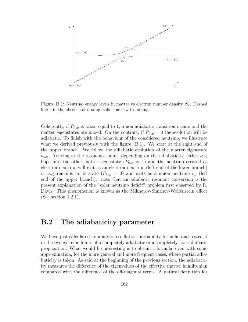
Figure B.1: Neutrino energy levels in matter vs electron number density Ne. Dashedline – in the absence of mixing, solid line – with mixing.
Coherently, if Phop is taken equal to 1, a non adiabatic transition occurs and thematter eigenstates are mixed. On the contrary, if Phop = 0 the evolution will beadiabatic. To finish with the behaviour of the considered neutrino, we illustratewhat we derived previously with the figure (B.1). We start at the right end ofthe upper branch. We follow the adiabatic evolution of the matter eigenstateνm2. Arriving at the resonance point, depending on the adiabaticity, either νm2
hops into the other matter eigenstate (Phop = 1) and the neutrino created aselectron neutrino will exit as an electron neutrino (left end of the lower branch)or νm2 remains in its state (Phop = 0) and exits as a muon neutrino νµ (leftend of the upper branch). note that an adiabatic resonant conversion is thepresent explanation of the ”solar neutrino deficit” problem first observed by R.Davis. This phenomenon is known as the Mikheyev-Smirnov-Wolfenstein effect(See section 1.2.1).
B.2 The adiabaticity parameter
We have just calculated an analytic oscillation probability formula, and tested itin the two extreme limits of a completely adiabatic or a completely non-adiabaticpropagation. What would be interesting is to obtain a formula, even with someapproximation, for the more general and more frequent cases, where partial adia-baticity is taken. As said at the beginning of the previous section, the adiabatic-ity measures the difference of the eigenvalues of the effective matter hamiltoniancompared with the difference of the off-diagonal terms. A natural definition for
162
the adiabaticity parameter is consequently:
γ =|Em1 −Em2||2θm(t)|
(B.19)
A similar problem is actually well known in atomic physics. In such a context,the hopping probability has been calculated by Landau and Zener in 1932 and intheir approximation one obtains:
Phop ≃ e−π2γr (B.20)
where γr, the adiabaticity evaluated at the resonance point, is:
γr =sin2 2θV
cos 2θV
∆m2
2E
∣
∣
∣
∣
d lnNe(t)
dt
∣
∣
∣
∣
−1
t=tr
(B.21)
B.3 The Landau-Zener formula
Considering the crossing of a polar and homopolar state of a molecule Landauand Zener, in 1932, independently derived, with some approximations, an ana-lytical formula for non-adiabatic crossing probability. About some 50 years laterpeople realised the importance of this formula in neutrino physics. We followan approach similar to Zener derivation to demonstrate the formula, adapted forneutrinos. Let us rewrite the effective matter Hamiltonian in the flavour basis:
Hfl =
(
−∆m2
4Ecos 2θV +
√2
2GFNe
∆m2
4Esin 2θV
∆m2
4Esin 2θV
∆m2
4Ecos 2θV −
√2
2GFNe
)
(B.22)
=
(
H1 H12
H12 H2
)
To derive such formula we consider that the region of transition we are interestedin is so small that H1 −H2 =
√2GF Ne = −α t can be approximated to a linear
function. This assumption is the same that making a Taylor development to thefirst order of Ne(t) at the time of resonance t = tr:
Ne(t) ≃ Ne(tr) +dNe(t)
dt|t=tr(t− tr) (B.23)
In its paper Zener was considering another approximation H12 = 0, but in ourcase, this is true without any approximation since θV is constant. Considering aneutrino state |ν(t)〉 = Ce(t)|νe〉 + Cµ(t)|νµ〉, the evolution equation we have tosolve is:
id
dt
(
Ce
Cµ
)
=
(
−∆m2
4Ecos 2θV +
√2
2GFNe
∆m2
4Esin 2θV
∆m2
4Esin 2θV
∆m2
4Ecos 2θV −
√2
2GFNe
)
(
Ce
Cµ
)
.
(B.24)
163
We can always redefine the Ce(t) and Cµ(t) functions modulo a phase, thus forpractical purpose we actually solve the following equation:
id
dt
(
Cee−i∫
H1(t)dt
Cµe−i∫
H2(t)dt
)
=
(
−∆m2
4Ecos 2θV +
√2
2GFNe
∆m2
4Esin 2θV
∆m2
4Esin 2θV
∆m2
4Ecos 2θV −
√2
2GFNe
)
(
Cee−i∫
H1(t)dt
Cµe−i∫
H2(t)dt
)
. (B.25)
This relation reduces to two simultaneous first order differential equations forCe(t) and Cµ(t):
H12Ce ei∫
(H2(t)−H1(t))dt = iCµ (B.26)
H12 Cµ e−i∫
(H2(t)−H1(t))dt = iCe
We impose the initial conditions we are interested in: Ce(ti) = 0 and |Cµ(ti)| = 1(i.e a νµ created initially). Combining those two equations and defining H12 = fwe find:
Ce(t)− i αt Ce(t) + f 2Ce(t) = 0 (B.27)
The substitution
Ce(t) = U1 e−i∫
(H2(t)−H1(t))dt (B.28)
reduces Eq.(B.27) to the Weber3 equation:
d2U1
dt2+
(
α2
4t2 − iα
2+ f 2
)
U1(t) = 0 (B.29)
A last redefinition of the variables:
z = α12 e−iπ/4t (B.30)
n = if 2/α
allows us to put Eq.(B.29) in the standard form:
d2U1
dz2+
(
−z2
4+ n+
1
2
)
U1(z) = 0 (B.31)
The Weber function D−n−1(iz) is a particular solution of this equation whichvanishes for infinite z along the directions ∞ exp(−i3π
4) and ∞ exp(−iπ
4). Hence
the solution satisfies the first boundary condition:
U1(z) = A±D−n−1(∓ iz), α ≷ 0 (B.32)
3A definition of a general Weber equation is d2fdz2 +
(
z2
4 − a)
f = 0
164
The initial conditions yield:
|A±|2 = γ e−πγ
2 (B.33)
By using its asymptotic value
limR→∞
D−n−1(i R e−i 3π
4 ) = ei 3π4
(n+1)eiR2/4R−n−1 +
√2π
Γ(n+ 1)e
14πnieiR2/4Rn (B.34)
we obtain4
|Ce(∞)|2 = Ce(∞)C∗e (∞) (B.35)
= U1(∞)U∗1 (∞) = |A±|2|D−n−1(i R e
i 3π4 )|2
=2πe
−πγ2 |A±|2
Γ(iγ + 1)Γ(−iγ + 1)=
2πγe−πγ
Γ(iγ + 1)Γ(−iγ + 1)
= 2e−πγ sinh(πγ) = 1− e−2πγ = 1− |Cµ(∞)|2
Therefore, the hopping probability is P = e−2πγ with
γ =H2
12
| ddt
(H1 −H2)|=
sin2 2θ0cos 2θ0
∆m2
4E
∣
∣
∣
∣
d lnNe(t)
dt
∣
∣
∣
∣
−1
t=tr
(B.36)
4Using the relation Γ(iγ + 1) = iγ Γ(iγ) = (iγ)! and |(iγ)!|−2 = sinh(πγ)/(πγ).
165

166
Appendix C
Several possible formalisms forthe neutrino evolution equations
In the study of the neutrino propagation, people are indistinctly using at least fourkinds of formalism, all perfectly equivalent, to describe the evolution of neutrinos:the Schrodinger equation for wave functions, the Schrodinger equation for theevolution operators, the Liouville-Von Neumann equation for the density matrix,and finally polarization vectors. Each of these formalisms are useful dependingon the specific problem to tackle. Wave functions may appear more natural touse, but density matrices are more compact. Eventually, the polarization vectorformalism is currently the best way to interpret the complex behavior of neutrinosin supernovae when they experience neutrino-neutrino interactions. We discusshere only the vacuum case for simplicity . However the discussion can be easilyextended to the case where matter and neutrino-neutrino interactions are present.
C.1 The Schrodinger equation for wave func-
tions
The evolution equation of neutrinos is actually a Schrodinger-like equation be-cause, unlike the Schrodinger equation, we are concerned with flavor evolution atfixed energy (or fixed momentum) of relativistic leptons. The evolution equationin vacuum in the flavour basis is then:
i∂
∂t
Ψe
Ψµ
Ψτ
=
T23T13T12
E1 0 00 E2 00 0 E3
T †12T
†13T
†23
Ψe
Ψµ
Ψτ
, (C.1)
where T23, T13 and T12 where given in the first chapter. As said in the previ-ous appendix, for antineutrinos a global minus sign appear, the equation (C.1)
167
becomes:
−i ∂∂t
Ψe
Ψµ
Ψτ
=
T23T13T12
E1 0 00 E2 00 0 E3
T †12T
†13T
†23
Ψe
Ψµ
Ψτ
, (C.2)
If we take the complex conjugate of Eq.(C.2) and redefine the antineutrino wavefunctions as Ψ
∗α = ψα then we’ll obtain:
i∂
∂t
ψe
ψµ
ψτ
=
T23T∗13T12
E1 0 00 E2 00 0 E3
T †12T
†13
∗T †
23
ψe
ψµ
ψτ
. (C.3)
The evolution equation is the same for neutrinos and antineutrinos except thatthe c.c. of T13 is taken for antineutrinos, this is the reason why the sign of δ, theCP-violating phase, has to be changed for antineutrinos.
C.2 The Schrodinger equation for evolution op-
erators
This is a equivalent way to express the previous equation on a matrix formcontaining all different initial conditions. The evolution operator U(t, 0) links theneutrino wave functions at a given time t to the initial neutrino wave functionscreated at time t = 0.
ψe(t)ψµ(t)ψτ (t)
= U(t, 0)
ψe(0)ψµ(0)ψτ (0)
, (C.4)
where
U(t, 0) =
Uee Ueµ Ueτ
Uµe Uµµ Uµτ
Uτe Uτµ Uττ
. (C.5)
To understand what’s representing the Uij coefficient, let’s take a physical casewhere a electron neutrino is initially created:
ψe(0)ψµ(0)ψτ (0)
=
100
. (C.6)
Replacing Eq.(C.6) in Eq.(C.4), one obtains:
ψe,e(t)ψµ,e(t)ψτ,e(t)
=
Uee
Uµe
Uτe
, (C.7)
168
where the double subscripts corresponds to the initial state of the consideredsystem. Therefore, |ψe,e(t)|2 = |Uee|2 = P (νe → νe), which is the probability to goto the state νe starting with the initial state where a νe has been created. Finally,the Schrodinger equation that contains all three initial states of a supernovaenvironment where all the neutrinos are created is:
i∂
∂t
Uee Ueµ Ueτ
Uµe Uµµ Uµτ
Uτe Uτµ Uττ
= H
Uee Ueµ Ueτ
Uµe Uµµ Uµτ
Uτe Uτµ Uττ
, (C.8)
where H is the hamiltonian of the system.
C.3 The Liouville-Von Neumann equation: the
density matrix formalism
The Liouville-Von Neumann equation describes the evolution of the density ma-trices The density matrix can be used in two cases : like wave functions one canconsider pure quantum states like Eq.(C.6), or one can consider superimposedstates or statistical mixture of states. This formalism is useful for the descrip-tion of oscillations of neutrino ensembles with more than one initial flavour withpossible loss of coherence, like in the environment of the early Universe.
The pure states
By definition, in a pure state, the description of the system is given by a statevector that can be expanded on a basis of a finite dimensional Hilbert space| un >, and
| ψ(t) > =∑
n
cn(t) | un > with∑
n
| cn(t) |2 = 1 (C.9)
The coefficients cn are probability amplitudes, and such amplitudes can interferejust as for neutrinos. The temporal evolution of the state vector is given by theSchrodinger equation:
id
dt| ψ(t) >= H | ψ(t) > (C.10)
where H is the hamiltonian of the system. We can then define the density oper-ator by:
ρ(t) =| ψ(t) >< ψ(t) |=∑
n,p
c∗ncp | up >< un | . (C.11)
169
This is the hermitian projection operator associated to the state describing thesystem. Note that any arbitrary phase present in the previous formalism doesnot appear in the density operator. Its matrix elements are :
ρpn =< up | ρ | un >= c∗ncp. (C.12)
For a pure state, the density matrix has the following properties:
1. Tr(ρ(t)) = 1
2. ρ†(t) = ρ(t)
3. ρ2(t) = ρ(t);
which express the probability conservation, the fact that ρ is hermitian, and aprojection operator. Finally, its time evolution is given by the Liouville-VonNeumann equation:
id
dtρ =
[
H, ρ]
. (C.13)
As an example, let us consider the case of a two-flavour neutrino system in vac-uum. As previously shown one can decompose the flavour state vector on thebasis of the eigenvectors of the Hamiltonian, namely in our case, the mass basis| νi > with i = 1, 2. For a flavour α, one has | ψνα
>= Uα1 | ν1 > +Uα2 | ν2 >with the lepton mixing matrix U defined by:
U =
(
cos θV sin θV
− sin θV cos θV
)
, (C.14)
θV being the vacuum mixing angle. Since the mass basis corresponds to theeigenvectors, the | νi > just acquires a phase factor | νi(t) >= e−iEit | νi(0) >.
At time t the state for a neutrino created as a να will be:
| ψνα(t) >= Uα1e
−iE1t | ν1 > +Uα2e−iE2t | ν2 >
and therefore the corresponding density matrix operator writes in the mass basis:
ρνα= | ψνα
(t) >< ψνα(t) |
= ρ11 | ν1 >< ν1 | + ρ22 | ν2 >< ν2 | + ρ12 | ν1 >< ν2 | + ρ21 | ν2 >< ν1 |(C.15)
In a matrix form one rewrites:
ρνα=
(
ρ11 ρ12
ρ21 ρ22
)
, (C.16)
170
since we have in this case:
ρii(t) = < νi | ρ | νi >= ρii(0) =| Uα1 |2 (C.17)
ρij(t) = < νi | ρ | νj >= ρij(0)e−i(Ei−Ej)t = UαiU∗αje
−i(Ei−Ej)t (C.18)
The diagonal terms called ”population” ρii are constant and the non-diagonalterms ρij (with i 6= j) called ”coherence” are oscillatingat the Bohr frequence ofthe considered transition. Finally, to calculate the survival probability of the νe
neutrino within the density matrix formalism is given by:
P (νe → νe) = < ψνe| ρ | ψνe
>
= < ψνe| (ρ11 cos θ0 | ν1 > +ρ22 sin θ0 | ν2 > + ρ12 sin θ0 | ν1 > + ρ21 cos θ0 | ν2 >)
= cos4 θ0 + sin4 θ0 + cos2 θ0 sin2 θ0(e−i(E1−E2)t + e−i(E2−E1)t)
= 1 + 2 cos2 θ0 sin2 θ0 (cos((E2 − E1)t)− 1)
= 1− sin2 2θ0 sin2
(
(E2 −E1)t
2
)
(C.19)
The statistical mixed states
In certain environments one can be interested to describe the statistical distribu-tion of the states. This is the case for neutrinos e.g in the Early Universe environ-ment, where they are at thermal equilibrium and therefore follow the Fermi-Diracstatistics. To neutrinos νe, νµ, ντ is respectively associated the Fermi-Dirac dis-tribution fνe
, fνµ, fντ
respectively. It is thus interesting to use the density matrix
formalism. If we take the mean value of an observable A we obtain:
< A >=∑
α=e,µ,τ
fνα< ψνα
| A | ψνα>=
∑
α=e,µ,τ
fναTr(ρνα
A) = Tr(ρmA) (C.20)
The statistical mixture of states can be described, with the same rule of calcu-lation that the mean values for the pure states, by the ”mean” density matrix,average of the different density matrices of the system studied:
ρm =∑
α=e,µ,τ
fναρνα
(C.21)
To finish with the example of the Early Universe environment, the density matrixrepresenting the mixed ensemble of single neutrino states all with momentum pcan be written as the incoherent sum
ρpd3p =
∑
α=e,µ,τ
dnνα| ψνα
>< ψνα|, (C.22)
where dnναis the local differential number density of να neutrinos with momen-
tum p in the d3p interval.
171
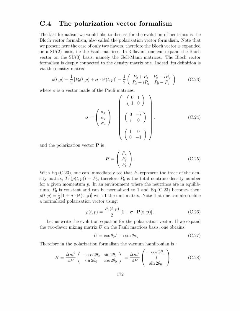
C.4 The polarization vector formalism
The last formalism we would like to discuss for the evolution of neutrinos is theBloch vector formalism, also called the polarization vector formalism. Note thatwe present here the case of only two flavors, therefore the Bloch vector is expandedon a SU(2) basis, i.e the Pauli matrices. In 3 flavors, one can expand the Blochvector on the SU(3) basis, namely the Gell-Mann matrices. The Bloch vectorformalism is deeply connected to the density matrix one. Indeed, its definition isvia the density matrix:
ρ(t, p) =1
2[P0(t, p) + σ ·P(t, p)] =
1
2
(
P0 + Pz Px − iPy
Px + iPy P0 − Pz
)
(C.23)
where σ is a vector made of the Pauli matrices.
σ =
σx
σy
σz
=
(
0 11 0
)
(
0 −ii 0
)
(
1 00 −1
)
. (C.24)
and the polarization vector P is :
P =
Px
Py
Pz
. (C.25)
With Eq.(C.23), one can immediately see that P0 represent the trace of the den-sity matrix, Tr(ρ(t, p)) = P0, therefore P0 is the total neutrino density numberfor a given momentum p. In an environment where the neutrinos are in equilib-rium, P0 is constant and can be normalized to 1 and Eq.(C.23) becomes then:ρ(t, p) = 1
2[1 + σ ·P(t,p)] with 1 the unit matrix. Note that one can also define
a normalized polarization vector using:
ρ(t, p) =P0(t, p)
2[1 + σ ·P(t,p)] . (C.26)
Let us write the evolution equation for the polarization vector. If we expandthe two-flavor mixing matrix U on the Pauli matrices basis, one obtains:
U = cos θ0I + i sin θσy (C.27)
Therefore in the polarization formalism the vacuum hamiltonian is :
H =∆m2
4E
(
− cos 2θ0 sin 2θ0sin 2θ0 cos 2θ0
)
≡ ∆m2
4E
− cos 2θ00
sin 2θ0
. (C.28)
172
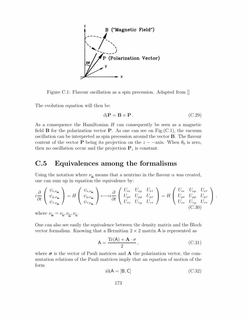
Figure C.1: Flavour oscillation as a spin precession. Adapted from []
The evolution equation will then be:
∂tP = B×P . (C.29)
As a consequence the Hamiltonian H can consequently be seen as a magneticfield B for the polarization vector P. As one can see on Fig.(C.1), the vacuumoscillation can be interpreted as spin precession around the vector B. The flavourcontent of the vector P being its projection on the z − −axis. When θ0 is zero,then no oscillation occur and the projection Pz is constant.
C.5 Equivalences among the formalisms
Using the notation where να means that a neutrino in the flavour α was created,one can sum up in equation the equivalence by:
i∂
∂t
ψe,να
ψµ,να
ψτ,να
= H
ψe,να
ψµ,να
ψτ,να
←→i ∂∂t
Uee Ueµ Ueτ
Uµe Uµµ Uµτ
Uτe Uτµ Uττ
= H
Uee Ueµ Ueτ
Uµe Uµµ Uµτ
Uτe Uτµ Uττ
.
(C.30)where να = νe, νµ, ντ .
One can also see easily the equivalence between the density matrix and the Blochvector formalism. Knowing that a Hermitian 2× 2 matrix A is represented as
A =Tr(A) + A · σ
2, (C.31)
where σ is the vector of Pauli matrices and A the polarization vector, the com-mutation relations of the Pauli matrices imply that an equation of motion of theform
i∂tA = [B,C] (C.32)
173
is represented by∂tTr(A) = 0 and ∂tA = B×C . (C.33)
Therefore it is straightforward to see that the Liouville Von-Neumann equation
i∂tρ = [H, ρ] (C.34)
gives in the Pauli matrices representation:
∂tTr(ρ) = 0 and ∂tρ = H× ρ , (C.35)
and translates in the polarization form into:
∂tTr(P0) = 0 and ∂tP = B×P , (C.36)
where B corresponds to the Hamiltonian H = 2H expanded on the Pauli matricesbasis. The flavor oscillation which can be calculated using Eq.(C.8) or Eq.(C.13)are fully analogous to the spin precession in a magnetic field. Here, B plays therole of a ”magnetic field” and P that of a ”spin vector”. If we define the densitymatrix in two flavours (νe and νµ) through the wave functions describing theneutrino states in the flavour basis by the following equations :
ρνα=
(
ρνeνeρνeνµ
ρνµνeρνµνµ
)
=
(
| ψe |2 ψeψ∗µ
ψ∗eψµ | ψµ |2
)
, (C.37)
then the polarization vector writes :
P =
2Re(ψ∗eψµ)
2Im(ψ∗eψµ)
| ψe |2 − | ψµ |2
. (C.38)
Consequently, ρνeνe=| ψe |2= 1
2(1 + Pz) and ρνµνµ
=| ψµ |2= 12(1 − Pz) give the
probability for the neutrino to be measured as νe or νµ respectively.
174
Appendix D
Some details concerning theneutrino-neutrino calculations
In this appendix, we develop the different calculation steps that are needed todescribe and interpret the neutrino-neutrino interaction and its consequences onthe neutrino evolution in the supernova environment.
D.1 The differential number density of neutri-
nos
We consider the differential number density of neutrinos dnνα(q) at radius r which
has the contribution from all να with energy q which propagate in directionswithin the range between q and q + dq.
Following [52] if we define jνα(q) as the number flux of να with energy q
emitted in any direction at the neutrino sphere. The number of neutrinos goingoutwards radially through the differential area R2
ν d(cos Θ)dΦ on the neutrinosphere surface per unit time is
dNνα,E = jνα(q)R2
ν d(cos Θ)dΦ (D.1)
Since we follow neutrinos going through this differential area but going towardsthe point P on Fig.(5.2), we need to multiply this expression by a geometricfactor cosϑ0 and consequently we obtain:
dNνα,P = jνα(q) cosϑ0R
2ν d(cos Θ)dΦ (D.2)
Another way to express this quantity is to look at the number of neutrinos arrivingon point P with angle ϑ with respect to the z–axis within the range of thedifferential area (l − l0)2d(cosϑ)dφ, and we obtain:
dNνα,P = jνα(q)(l − l0)2 d(cosϑ)dφ = (l − l0)2dnνα
(q) (D.3)
175
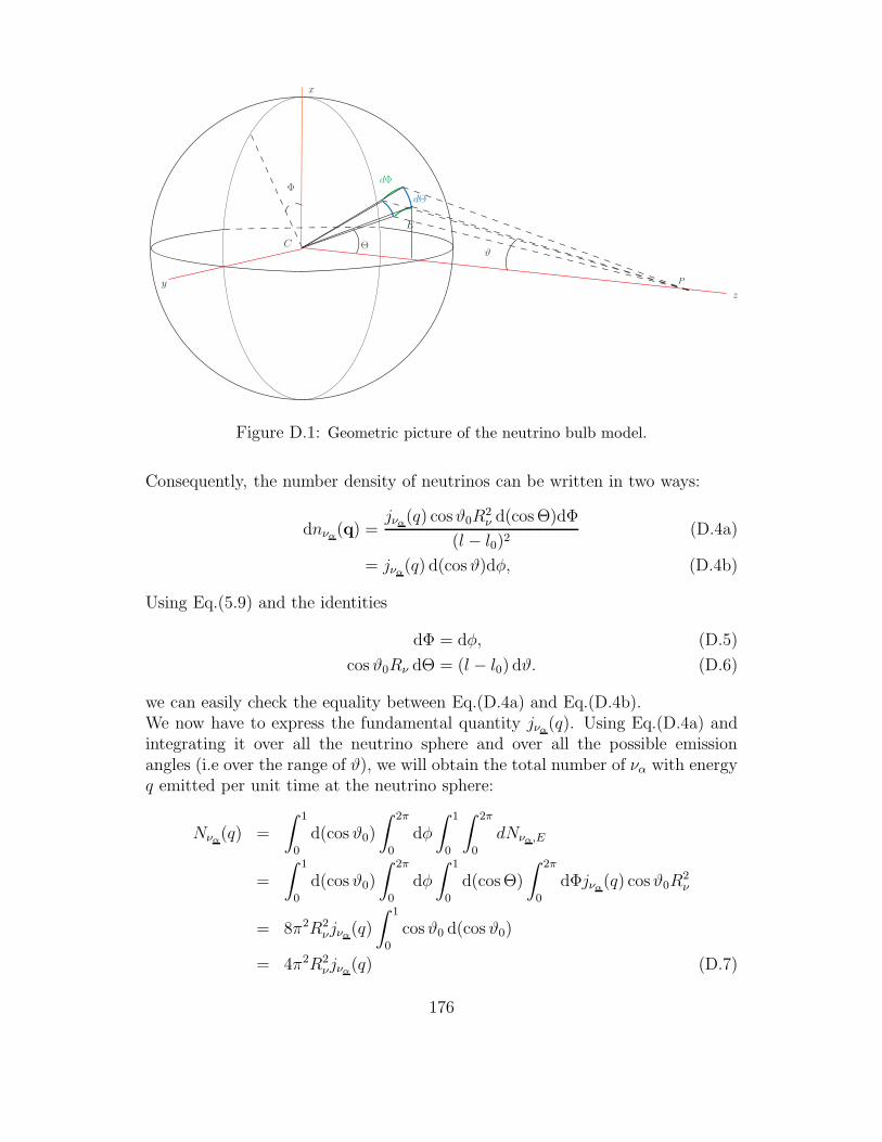
ΦdΦ
dΘ
x
zy
Θϑ
P
E
C
Figure D.1: Geometric picture of the neutrino bulb model.
Consequently, the number density of neutrinos can be written in two ways:
dnνα(q) =
jνα(q) cosϑ0R
2ν d(cos Θ)dΦ
(l − l0)2(D.4a)
= jνα(q) d(cosϑ)dφ, (D.4b)
Using Eq.(5.9) and the identities
dΦ = dφ, (D.5)
cosϑ0Rν dΘ = (l − l0) dϑ. (D.6)
we can easily check the equality between Eq.(D.4a) and Eq.(D.4b).We now have to express the fundamental quantity jνα
(q). Using Eq.(D.4a) andintegrating it over all the neutrino sphere and over all the possible emissionangles (i.e over the range of ϑ), we will obtain the total number of να with energyq emitted per unit time at the neutrino sphere:
Nνα(q) =
∫ 1
0
d(cos ϑ0)
∫ 2π
0
dφ
∫ 1
0
∫ 2π
0
dNνα,E
=
∫ 1
0
d(cos ϑ0)
∫ 2π
0
dφ
∫ 1
0
d(cos Θ)
∫ 2π
0
dΦjνα(q) cosϑ0R
2ν
= 8π2R2νjνα
(q)
∫ 1
0
cosϑ0 d(cos ϑ0)
= 4π2R2νjνα
(q) (D.7)
176
Because this flux can also be expressed as
Nνα(q) =
Lνα
〈Eνα〉fνα
(q), (D.8)
where Lνα, 〈Eνα
〉 and fνα(q) are the energy luminosity, average energy and nor-
malized energy distribution function of να, respectively. Therefore one has
jνα(q) =
Lνα
4π2R2ν〈Eνα
〉fνα(q). (D.9)
Note that this formula applies both for neutrinos and antineutrinos. Finally, theneutrino-neutrino forward scattering Hamiltonian can be written as
Hνν =√
2GF
∑
α
[∫
ρνα(q′)(1− q · q′)dnνα
(q′)− ρνα(q′)(1− q · q′)dnνα
(q′)
]
dq′
(D.10)where q and q′ are the momentum of the neutrino of interest and that of the back-ground neutrino, respectively. As mentioned above, neutrinos of the same initialflavor, energy and emission angle have identical flavor evolution. Consequentlyone must have
ν(q) = ν(q, ϑ). (D.11)
Writing the vectors in the spherical coordinates and integrating it over the solidangle dq′ we obtain:∫
q · q′dq′ =
∫
[sin ϑ sinϑ′(sinφ sinφ′ + cosφ cosφ′) + cosϑ cosϑ′] d(cosϑ′)dφ′
(D.12)Because as said before the problem has a cylindrical symmetry around the z–axis,the terms proportional to sin φ′ and cosφ′ will average to zero when integratingon the azimuthal angle φ′:
∫
q · q′dq′ = 2π
∫
cosϑ cos ϑ′ d(cosϑ′) (D.13)
Using Eqs.(D.4b) ,(D.9) and (D.12), we finally obtain:
Hνν =
√2GF
2πR2ν
∑
α
∫
(1− cosϑ cosϑ′) (D.14)
[
ρνα(q′, ϑ′)fνα
(q′)Lνα
〈Eνα〉 − ρ
∗να
(q′, ϑ′)fνα(q′)
Lνα
〈Eνα〉
]
d(cos ϑ′)dq′.
This is the multi-angle neutrino-neutrino interaction Hamiltonian where, in ad-dition to the momentum, we also integrate over the emission angle ϑ′ when weconsider the direction of interaction given by ϑ.
177
D.2 The rotating frame
The idea of changing to a new frame is to keep the same form than the previousevolution equations. We start from the equation of motions for a neutrino andan antineutrino of a given energy ω, using the polarization vector formalism:
∂tP =[
+ωB + λL + µ(
P− P)]
×P ,
∂tP =[
−ωB + λL + µ(
P− P)]
× P . (D.15)
where L = (0, 0, 1). We include here matter effects caused by charged leptons.Since the case without matter has been well understood and studied, it wouldbe interesting to get the same equations than without matter, by working in anew referential. Focusing on the neutrinos (the derivation is exactly the same forantineutrinos), we impose
∂tP− λL×P =
(Px + λPy)x
(Py − λPx)y
Pzz
≡
Puu
Pvv
Pww
. (D.16)
where (u,v,w) is the new referential orthonormal basis. Since λ, the coefficientassociated with matter, does not modify the z component, the relation betweenthe previous referential and the new one is in its most general form:
xyz
= R
uvw
=
a b 0c d 00 0 1
uvw
. (D.17)
Moreover, we know that the polarization vector is real1, the norm of each coordi-nate has to be equal to 12, and the scalar product between two coordinates hasto be zero3. These conditions imply:
R =
cosα(t) sinα(t) 0− sinα(t) cosα(t) 0
0 0 1
(D.18)
Thus we deduct that the basis changing matrix is a rotation matrix of angle α(t)4
and of z axis. In the new referential the P vector writes:
PxxPyyPzz
⇒
(cosα(t)Px − sinα(t)Py)u(sinα(t)Px + cosα(t)Py)v
Pzw
. (D.19)
1 a,b,c and d are real.2 a2 + b2 = 1 and c2 + d2 = 1.3 ac + bd = 0.4 Since matter is changing with time, we take α as a function of time
178
Since we want in the new referential the same equations than previously withoutmatter, we have the following relation:
Pu = cosα(t)Px − sinα(t)Py (D.20)
Pv = sinα(t)Px + cosα(t)Py
and consequently
Pu = (Px − αPy) cosα(t)− (αPx + Py) sinα(t) (D.21)
Pv = (Px − αPy) sinα(t) + (αPx + Py) cosα(t)
Expressing Puu and Pvv in the previous referential and using Eq.(D.16), weobtain
Pu cosα(t) + Pv sinα(t) = Px + λ Py (D.22)
which yields:α(t) = −λ and therefore α(t) = −λ t+cst. Since the two referentials coincide ini-tially, i.e α(t = 0) = 0, we have: α = −λ t. Consequently, in the new referential,the equations of motion would be exactly the same than without matter:
∂tPω =[
+ωB(t) + µ(
Pω − Pω
)]
×Pω ,
∂tPω =[
−ωB(t) + µ(
Pω − Pω
)]
× Pω . (D.23)
except that the magnetic field B(t) is now time dependent as:
B(t) =
sin(2θ0) cos(−λt)sin(2θ0) sin(−λt)− cos(2θ0)
. (D.24)
We name this new referential, the rotating frame.
D.3 The corotating frame and the adiabaticity
The corotating frame
To express the new E.O.M. in this frame, we perform a similar derivation thanthe one made previously to make disappear the matter effect. We define the newframe such that D is a constant vector in this frame.
∂tD− ωcB×D =
(Dx + ωcDy)x
(Dy − ωcDx)y
Dzz
=
0u0v0w
=
Duu
Dvv
Dww
. (D.25)
Using the same relation to move from one basis to another than before (seeEq.(D.18)) with α(t) = −ωct one obtains:
Pxx
Pyy
Pzz
=
(Pu + αPv)u
(Pv − αPu)v
Pww
+
αPvu−αPuv
0w
. (D.26)
179
We can express the second vector of the r.h.s of Eq.(D.26) as a vector product:
αPvu−αPuv
0w
= −α
0u0v1w
×
PuuPvvPww
. (D.27)
The adiabaticy notion within the polarization vector formalism
In this subsection, we come back on the adiabaticity notion: It is also possibleto measure adiabaticity like it was previously done when we studied the MSWresonance, by defining the adiabaticity parameter has the ratio of the off diagonalterm of the instantly diagonalized Hamiltonian over the diagonal terms of thesame Hamiltonian. Recalling that the off diagonal terms of a matrix correspondto the transverse term in the polarization vector formalism, one can define themedium mixing angle by5
cos θω ≡ Hω⊥/Hω (D.28)
Thus, the speed for the Hω evolution in the co-rotating plane is dθω/dt, while Pω
precesses with speed Hω. The evolution is adiabatic if the adiabaticity parameterγω ≡ |dθω/dt|H−1
ω ≪ 1.Let us now look to the link between the adiabaticity notion and the consequenceson the relevant variables. If we insert Eq.(5.60), in the E.O.M. given by Eq.(5.59)we obtain
∂tHω(µ) = ∂t(µD) = 0 , (D.29)
which is satisfied exactly if ∂tµ = 0 and ∂tD = 0. That is, the medium hasconstant neutrino density and the difference vector does not change. The factthat µ should be independent of time is coherent with the previous assumptionwhich considered a µ changing slowly with time. The same reasoning appliesfor the second condition which says that D should be independent of time. Inthe adiabatic approximation we supposed a slow variation for Hω and a fortiorifor the Pω which follow Hω. We see therefore a perfect coherence between thedifferent assumptions taken and the solutions yielded by the E.O.M. with suchassumptions.
5To obtain such formula we considered that the flavour basis almost coincide with themass basis by taking a small vacuum mixing angle (which is quite correct for θ13), and sincethe in-medium mixing angle near a SN core is small, the mass basis almost coincide withthe interaction/medium basis. Consequently, we considered that the flavour basis and theinteraction basis almost coincide too. That is why we can define the in-medium mixing anglewith Hω written in the flavour basis.
180
Bibliography
[1] Kevork Abazajian, Nicole F. Bell, George M. Fuller, and Yvonne Y. Y.Wong. Cosmological lepton asymmetry, primordial nucleosynthesis, andsterile neutrinos. Phys. Rev., D72:063004, 2005.
[2] Kevork N. Abazajian, John F. Beacom, and Nicole F. Bell. Stringent con-straints on cosmological neutrino antineutrino asymmetries from synchro-nized flavor transformation. Phys. Rev., D66:013008, 2002.
[3] Dzh. N. Abdurashitov et al. The Russian-American gallium experiment(SAGE) Cr neutrino source measurement. Phys. Rev. Lett., 77:4708–4711,1996.
[4] Q. R. Ahmad et al. Measurement of the charged current interactions pro-duced by B-8 solar neutrinos at the Sudbury Neutrino Observatory. Phys.Rev. Lett., 87:071301, 2001.
[5] M. H. Ahn et al. Indications of Neutrino Oscillation in a 250 km Long-baseline Experiment. Phys. Rev. Lett., 90:041801, 2003.
[6] Evgeny Khakimovich Akhmedov, Cecilia Lunardini, and Alexei Yu.Smirnov. Supernova neutrinos: Difference of nu/mu - nu/tau fluxes andconversion effects. Nucl. Phys., B643:339–366, 2002.
[7] E. N. Alekseev, L. N. Alekseeva, V. I. Volchenko, and I. V. Krivosheina.POSSIBLE DETECTION OF A NEUTRINO SIGNAL ON 23 FEBRU-ARY 1987 AT THE BAKSAN UNDERGROUND SCINTILLATIONTELESCOPE OF THE INSTITUTE OF NUCLEAR RESEARCH. JETPLett., 45:589–592, 1987.
[8] Philip S. Amanik, George M. Fuller, and Benjamin Grinstein. Flavor chang-ing supersymmetry interactions in a supernova. Astropart. Phys., 24:160–182, 2005.
[9] C. Amsler et al. Review of particle physics. Phys. Lett., B667:1, 2008.
181
[10] Hajime Anada and Haruhiko Nishimura. COHERENCE CONDITIONFOR RESONANT NEUTRINO OSCILLATIONS. Phys. Rev., D41:2379,1990.
[11] P. Anselmann et al. Solar neutrinos observed by GALLEX at Gran Sasso.Phys. Lett., B285:376–389, 1992.
[12] T. Araki et al. Measurement of neutrino oscillation with KamLAND: Evi-dence of spectral distortion. Phys. Rev. Lett., 94:081801, 2005.
[13] F. Ardellier et al. Double Chooz: A search for the neutrino mixing angletheta(13). 2006.
[14] C. Arpesella et al. Direct Measurement of the Be-7 Solar Neutrino Fluxwith 192 Days of Borexino Data. Phys. Rev. Lett., 101:091302, 2008.
[15] C. Arpesella et al. First real time detection of Be7 solar neutrinos byBorexino. Phys. Lett., B658:101–108, 2008.
[16] C. Athanassopoulos et al. Evidence for anti-nu/mu –¿ anti-nu/e oscillationfrom the LSND experiment at the Los Alamos Meson Physics Facility.Phys. Rev. Lett., 77:3082–3085, 1996.
[17] C. Athanassopoulos et al. Evidence for nu/mu –¿ nu/e neutrino oscillationsfrom LSND. Phys. Rev. Lett., 81:1774–1777, 1998.
[18] D. Autiero et al. Large underground, liquid based detectors for astro-particle physics in Europe: scientific case and prospects. JCAP, 0711:011,2007.
[19] John N. Bahcall. Standard solar models. Nucl. Phys. Proc. Suppl., 77:64–72, 1999.
[20] John N. Bahcall, P. I. Krastev, and A. Yu. Smirnov. Where do we standwith solar neutrino oscillations? Phys. Rev., D58:096016, 1998.
[21] A. B. Balantekin, J. H. de Jesus, R. Lazauskas, and C. Volpe. A conservedvector current test using low energy beta- beams. Phys. Rev., D73:073011,2006.
[22] A. B. Balantekin, S. H. Fricke, and P. J. Hatchell. ANALYTICAL ANDSEMICLASSICAL ASPECTS OF MATTER ENHANCED NEUTRINOOSCILLATIONS. Phys. Rev., D38:935, 1988.
[23] A. B. Balantekin and G. M. Fuller. Supernova neutrino nucleus astro-physics. J. Phys., G29:2513–2522, 2003.
182
[24] A. B. Balantekin and Y. Pehlivan. Neutrino neutrino interactions and flavormixing in dense matter. J. Phys., G34:47–66, 2007.
[25] A. B. Balantekin and H. Yuksel. Neutrino mixing and nucleosynthesis incore-collapse supernovae. New J. Phys., 7:51, 2005.
[26] Akif Baha Balantekin, J. Gava, and C. Volpe. Possible CP-Violation effectsin core-collapse Supernovae. Phys. Lett., B662:396–404, 2008.
[27] A. Bandyopadhyay et al. Physics at a future Neutrino Factory and super-beam facility. 2007.
[28] H. A. Bethe. Energy Production in Stars. Physical Review, 55:434–456,1939.
[29] Hans A. Bethe. Supernova 1987A: An Empirical and analytic approach.Astrophys. J., 412:192–202, 1993.
[30] Samoil M. Bilenky, C. Giunti, and W. Grimus. Phenomenology of neutrinooscillations. Prog. Part. Nucl. Phys., 43:1–86, 1999.
[31] R. M. Bionta et al. Observation of a Neutrino Burst in Coincidence withSupernova SN 1987a in the Large Magellanic Cloud. Phys. Rev. Lett.,58:1494, 1987.
[32] Mattias Blennow, Alessandro Mirizzi, and Pasquale D. Serpico. Nonstan-dard neutrino-neutrino refractive effects in dense neutrino gases. Phys.Rev., D78:113004, 2008.
[33] F. J. Botella, C. S. Lim, and W. J. Marciano. RADIATIVE COR-RECTIONS TO NEUTRINO INDICES OF REFRACTION. Phys. Rev.,D35:896, 1987.
[34] Stephen J. Brice. MiniBooNE oscillation searches. J. Phys. Conf. Ser.,136:022026, 2008.
[35] Margaret E. Burbidge, G. R. Burbidge, William A. Fowler, and F. Hoyle.Synthesis of the elements in stars. Rev. Mod. Phys., 29:547–650, 1957.
[36] F. Reines F. B. Harrison H. W. Kruse C. L. Cowan, Jr. and A. D. McGuire.Detection of the Free Neutrino: A Confirmation. Science, 124:103, 1956.
[37] Christian Y. Cardall and George M. Fuller. Big-Bang Nucleosynthesis inLight of Discordant Deuterium Measurements. Astrophys. J., 472:435, 1996.
[38] GNO collaboration. GNO Solar Neutrino Observations: Results for GNOI.Physics Letter B, 490:16–26, 2000.
183
[39] The Borexino Collaboration. Measurement of the solar 8B neutrino fluxwith 246 live days of Borexino and observation of the MSW vacuum-mattertransition. 2008.
[40] Richard H. Cyburt, Brian D. Fields, Keith A. Olive, and Evan Skill-man. New BBN limits on Physics Beyond the Standard Model from He4.Astropart. Phys., 23:313–323, 2005.
[41] Basudeb Dasgupta and Amol Dighe. Phase effects in neutrino conversionsduring a supernova shock wave. Phys. Rev., D75:093002, 2007.
[42] Basudeb Dasgupta and Amol Dighe. Collective three-flavor oscillations ofsupernova neutrinos. Phys. Rev., D77:113002, 2008.
[43] Basudeb Dasgupta, Amol Dighe, and Alessandro Mirizzi. Identifying neu-trino mass hierarchy at extremely small theta(13) through Earth mattereffects in a supernova signal. Phys. Rev. Lett., 101:171801, 2008.
[44] Basudeb Dasgupta, Amol Dighe, Alessandro Mirizzi, and Georg G. Raffelt.Spectral split in prompt supernova neutrino burst: Analytic three-flavortreatment. Phys. Rev., D77:113007, 2008.
[45] Jr. Davis, Raymond, Don S. Harmer, and Kenneth C. Hoffman. Search forneutrinos from the sun. Phys. Rev. Lett., 20:1205–1209, 1968.
[46] A. de Bellefon et al. MEMPHYS: A large scale water Cerenkov detector atFrejus. 2006.
[47] Amol S. Dighe and Alexei Yu. Smirnov. Identifying the neutrino mass spec-trum from the neutrino burst from a supernova. Phys. Rev., D62:033007,2000.
[48] A. D. Dolgov et al. Cosmological bounds on neutrino degeneracy improvedby flavor oscillations. Nucl. Phys., B632:363–382, 2002.
[49] A. D. Dolgov, S. H. Hansen, and D. V. Semikoz. Non-equilibrium correc-tions to the spectra of massless neutrinos in the early universe. Nucl. Phys.,B503:426–444, 1997.
[50] A. D. Dolgov, S. H. Hansen, and D. V. Semikoz. Nonequilibrium correctionsto the spectra of massless neutrinos in the early universe. (Addendum).Nucl. Phys., B543:269–274, 1999.
[51] Huaiyu Duan, George M. Fuller, J. Carlson, and Yong-Zhong Qian. Coher-ent Development of Neutrino Flavor in the Supernova Environment. Phys.Rev. Lett., 97:241101, 2006.
184
[52] Huaiyu Duan, George M. Fuller, J Carlson, and Yong-Zhong Qian. Simula-tion of coherent non-linear neutrino flavor transformation in the supernovaenvironment. I: Correlated neutrino trajectories. Phys. Rev., D74:105014,2006.
[53] Huaiyu Duan, George M. Fuller, J. Carlson, and Yong-Zhong Qian. FlavorEvolution of the Neutronization Neutrino Burst from an O-Ne-Mg Core-Collapse Supernova. Phys. Rev. Lett., 100:021101, 2008.
[54] Huaiyu Duan, George M. Fuller, and Yong-Zhong Qian. Collective NeutrinoFlavor Transformation In Supernovae. Phys. Rev., D74:123004, 2006.
[55] Huaiyu Duan, George M. Fuller, and Yong-Zhong Qian. Stepwise SpectralSwapping with Three Neutrino Flavors. Phys. Rev., D77:085016, 2008.
[56] K. Eguchi et al. First results from KamLAND: Evidence for reactor anti-neutrino disappearance. Phys. Rev. Lett., 90:021802, 2003.
[57] J. Engel, G. C. McLaughlin, and C. Volpe. What can be learned with alead-based supernova-neutrino detector? Phys. Rev., D67:013005, 2003.
[58] A. Esteban-Pretel et al. Role of dense matter in collective supernova neu-trino transformations. Phys. Rev., D78:085012, 2008.
[59] A. Esteban-Pretel, R. Tomas, and J. W. F. Valle. Probing non-standardneutrino interactions with supernova neutrinos. Phys. Rev., D76:053001,2007.
[60] Andreu Esteban-Pretel, Sergio Pastor, Ricard Tomas, Georg G. Raffelt, andGunter Sigl. Decoherence in supernova neutrino transformations suppressedby deleptonization. Phys. Rev., D76:125018, 2007.
[61] Andreu Esteban-Pretel, Sergio Pastor, Ricard Tomas, Georg G. Raffelt,and Gunter Sigl. Mu-tau neutrino refraction and collective three-flavortransformations in supernovae. Phys. Rev., D77:065024, 2008.
[62] G. L. Fogli, E. Lisi, A. Marrone, A. Mirizzi, and I. Tamborra. Low-energyspectral features of supernova (anti)neutrinos in inverted hierarchy. Phys.Rev., D78:097301, 2008.
[63] G. L. Fogli, E. Lisi, A. Mirizzi, and D. Montanino. Probing supernova shockwaves and neutrino flavor transitions in next-generation water-Cherenkovdetectors. JCAP, 0504:002, 2005.
[64] Gianluigi L. Fogli, Eligio Lisi, Antonio Marrone, and Alessandro Mirizzi.Collective neutrino flavor transitions in supernovae and the role of trajec-tory averaging. JCAP, 0712:010, 2007.
185
[65] Gianluigi L. Fogli, Eligio Lisi, Alessandro Mirizzi, and Daniele Montanino.Damping of supernova neutrino transitions in stochastic shock-wave densityprofiles. JCAP, 0606:012, 2006.
[66] Y. Fukuda et al. Atmospheric muon-neutrino / electron-neutrino ratio inthe multiGeV energy range. Phys. Lett., B335:237–245, 1994.
[67] George M. Fuller, William A. Fowler, and Michael J. Newman. STELLARWEAK INTERACTION RATES FOR INTERMEDIATE MASS NUCLEI.2. A = 21 To A = 60. Astrophys. J., 252:715–740, 1982.
[68] Jerome Gava, James Kneller, Cristina Volpe, and G. C. McLaughlin. Adynamical collective calculation of supernova neutrino signals. Phys. Rev.Lett., 103:071101, 2009.
[69] Jerome Gava and Cristina Volpe. Collective neutrinos oscillation in matterand CP- violation. Phys. Rev., D78:083007, 2008.
[70] Xinheng Guo et al. A precision measurement of the neutrino mixing angletheta(13) using reactor antineutrinos at Daya Bay. 2007.
[71] W. Hampel et al. GALLEX solar neutrino observations: Results forGALLEX III. Phys. Lett., B388:384–396, 1996.
[72] Steen Hannestad, Georg G. Raffelt, Gunter Sigl, and Yvonne Y. Y. Wong.Self-induced conversion in dense neutrino gases: Pendulum in flavour space.Phys. Rev., D74:105010, 2006.
[73] S. H. Hansen, G. Mangano, A. Melchiorri, G. Miele, and O. Pisanti. Con-straining neutrino physics with BBN and CMBR. Phys. Rev., D65:023511,2002.
[74] K. Hirata et al. Observation of a Neutrino Burst from the Supernova SN1987a. Phys. Rev. Lett., 58:1490–1493, 1987.
[75] C. J. Horowitz and Gang Li. The mu and tau number of supernovae. Phys.Lett., B443:58–62, 1998.
[76] C. J. Horowitz and Gang Li. Charge conjugation violating interactions insupernovae and nucleosynthesis. Phys. Rev. Lett., 82:5198, 1999.
[77] Issei Kato. The K2K and T2K experiments. Nucl. Phys. Proc. Suppl.,168:199–201, 2007.
[78] Mathias Th. Keil, Georg G. Raffelt, and Hans-Thomas Janka. Monte Carlostudy of supernova neutrino spectra formation. Astrophys. J., 590:971–991,2003.
186
[79] James P. Kneller and Gail C. McLaughlin. Monte Carlo neutrino oscilla-tions. Phys. Rev., D73:056003, 2006.
[80] James P. Kneller and Gail C. McLaughlin. Three Flavor Neutrino Oscilla-tions in Matter: Flavor Diagonal Potentials, the Adiabatic Basis and theCP phase. 2009.
[81] James P. Kneller, Gail C. McLaughlin, and Justin Brockman. OscillationEffects and Time Variation of the Supernova Neutrino Signal. Phys. Rev.,D77:045023, 2008.
[82] James P. Kneller, Robert J. Scherrer, Gary Steigman, and Terry P. Walker.How Does CMB + BBN Constrain New Physics? Phys. Rev., D64:123506,2001.
[83] James M. Lattimer and A. Yahil. Analysis of the neutrino events fromsupernova 1987A. Astrophys. J., 340:426–434, 1989.
[84] Matthias Liebendoerfer, M. Rampp, H. Th. Janka, and A. Mezzacappa.Supernova Simulations with Boltzmann Neutrino Transport: A Comparisonof Methods. Astrophys. J., 620:840–860, 2005.
[85] C. Lunardini, Berndt Muller, and H. Th. Janka. Neutrino oscillation sig-natures of oxygen-neon-magnesium supernovae. Phys. Rev., D78:023016,2008.
[86] Cecilia Lunardini and Alexei Yu. Smirnov. Probing the neutrino masshierarchy and the 13-mixing with supernovae. JCAP, 0306:009, 2003.
[87] Z. Maki, M. Nakagawa, and S. Sakata. Remarks on the unified model ofelementary particles. Prog. Theor. Phys., 28:870, 1962.
[88] Gianpiero Mangano et al. Relic neutrino decoupling including flavour os-cillations. Nucl. Phys., B729:221–234, 2005.
[89] S. P. Mikheev and A. Yu. Smirnov. Resonance enhancement of oscillationsin matter and solar neutrino spectroscopy. Sov. J. Nucl. Phys., 42:913–917,1985.
[90] S. P. Mikheev and A. Yu. Smirnov. Resonance Oscillations of Neutrinos inMatter. Sov. Phys. Usp., 30:759–790, 1987.
[91] Dirk Notzold and Georg Raffelt. Neutrino Dispersion at Finite Temperatureand Density. Nucl. Phys., B307:924, 1988.
[92] Hiroshi Nunokawa, Stephen J. Parke, and Jose W. F. Valle. CP Violationand Neutrino Oscillations. Prog. Part. Nucl. Phys., 60:338–402, 2008.
187
[93] S. Nussinov. Solar Neutrinos and Neutrino Mixing. Phys. Lett., B63:201–203, 1976.
[94] Sergio Pastor and Georg Raffelt. Flavor oscillations in the supernova hotbubble region: Nonlinear effects of neutrino background. Phys. Rev. Lett.,89:191101, 2002.
[95] Sergio Pastor, Georg G. Raffelt, and Dmitry V. Semikoz. Physics of syn-chronized neutrino oscillations caused by self-interactions. Phys. Rev.,D65:053011, 2002.
[96] B. Pontecorvo. Mesonium and antimesonium. Sov. Phys. JETP, 6:429,1957.
[97] B. Pontecorvo. Inverse beta processes and nonconservation of lepton charge.Sov. Phys. JETP, 7:172–173, 1958.
[98] B. Pontecorvo. Neutrino experiments and the question of leptonic-chargeconservation. Sov. Phys. JETP, 26:984–988, 1968.
[99] Yong-Zhong Qian et al. A Connection between flavor mixing of cosmologi-cally significant neutrinos and heavy element nucleosynthesis in supernovae.Phys. Rev. Lett., 71:1965–1968, 1993.
[100] Yong-Zhong Qian and George M. Fuller. Matter enhanced anti-neutrinoflavor transformation and supernova nucleosynthesis. Phys. Rev., D52:656–660, 1995.
[101] Yong Zhong Qian and George M. Fuller. Neutrino-neutrino scattering andmatter enhanced neutrino flavor transformation in Supernovae. Phys. Rev.,D51:1479–1494, 1995.
[102] Georg G. Raffelt. Particle Physics from Stars. Ann. Rev. Nucl. Part. Sci.,49:163–216, 1999.
[103] Georg G. Raffelt and Alexei Yu. Smirnov. Adiabaticity and spectral splitsin collective neutrino transformations. Phys. Rev., D76:125008, 2007.
[104] Georg G. Raffelt and Alexei Yu. Smirnov. Self-induced spectral splits insupernova neutrino fluxes. Phys. Rev., D76:081301, 2007.
[105] Stuart Samuel. Neutrino oscillations in dense neutrino gases. Phys. Rev.,D48:1462–1477, 1993.
[106] Kate Scholberg. Atmospheric neutrinos at Super-Kamiokande. 1999.
[107] David N. Schramm and Michael S. Turner. Big-bang nucleosynthesis entersthe precision era. Rev. Mod. Phys., 70:303–318, 1998.
188
[108] G. Sigl and G. Raffelt. General kinetic description of relativistic mixedneutrinos. Nucl. Phys., B406:423–451, 1993.
[109] A. Yu. Smirnov. Neutrino mass and mixing: Toward the underlying physics.Prepared for Les Houches Summer School on Theoretical Physics: Session84: Particle Physics Beyond the Standard Model, Les Houches, France,1-26 Aug 2005.
[110] D. N. Spergel et al. First Year Wilkinson Microwave AnisotropyProbe (WMAP) Observations: Determination of Cosmological Parameters.Astrophys. J. Suppl., 148:175–194, 2003.
[111] Gary Steigman. Primordial nucleosynthesis: Successes and challenges. Int.J. Mod. Phys., E15:1–36, 2006.
[112] K. Takahashi, J. Witti, and H. T. Janka. Nucleosynthesis in neutrino-drivenwinds from protoneutron stars. 2. The R-process. Astron. Astrophys.,286:857, 1994.
[113] R. Tomas et al. Neutrino signatures of supernova shock and reverse shockpropagation. JCAP, 0409:015, 2004.
[114] T. Totani, K. Sato, H. E. Dalhed, and J. R. Wilson. Future detection ofsupernova neutrino burst and explosion mechanism. Astrophys. J., 496:216–225, 1998.
[115] Cristina Volpe. Topical review on ’beta-beams’. J. Phys., G34:R1–R44,2007.
[116] Walter Winter. How astrophysical neutrino sources could be used for earlymeasurements of neutrino mass hierarchy and leptonic CP phase. Phys.Rev., D74:033015, 2006.
[117] L. Wolfenstein. Neutrino oscillations in matter. Phys. Rev., D17:2369–2374,1978.
[118] S. E. Woosley and Robert D. Hoffman. The alpha-process and the r process.Astrophys. J., 395:202–239, 1992.
[119] S. E. Woosley, J. R. Wilson, G. J. Mathews, R. D. Hoffman, and B. S.Meyer. The r process and neutrino heated supernova ejecta. Astrophys. J.,433:229–246, 1994.
[120] Takashi Yoshida et al. Neutrino oscillation effects on supernova light ele-ment synthesis. Astrophys. J., 649:319–331, 2006.
189
RESUME DE LA THESE EN FRANCAIS
Le phenomene d’oscillation des neutrinos a ete decouvert en 1998 par l’experienceSuper-Kamiokande, 11 ans apres la premiere observation de neutrinos provenantd’une supernova (SN1987A). Ainsi, ce domaine s’est developpe grandement depuisune dizaine d’annees. Le sujet de cette these est l’etude, dans les contextes as-trophysique et cosmologique, de proprietes des neutrinos inconnues: la violationde CP et le troisieme angle de melange de la matrice MNSP. Nous avons montreanalytiquement, pour la premiere fois, les conditions dans lesquelles il peut yavoir des effets de la phase CP sur les flux de neutrinos dans l’etoile ainsi que surla fraction d’electrons, observable clef du processus-r. Les calculs numeriques, in-cluant le couplage a la matiere et l’interaction neutrino-neutrino non-lineaire, ontmontre des effets de plusieurs pourcents dans l’etoile et plus petits dans un ob-servatoire. Ensuite, nous avons etudie les consequences de la valeur du troisiemeangle, sur le flux d’antineutrinos a l’aide d’une simulation numerique dans l’etatde l’art, incluant l’interaction neutrino-neutrino ainsi qu’une densite de matieredynamique avec ondes de chocs. Une signature caracteristique de la hierarchie etde l’angle a ete trouvee, dans le signal des positrons, emis via le processus beta-inverse, dans un observatoire sur Terre. Enfin dans le contexte cosmologique, nousavons etudie l’impact de la phase de violation de CP sur le potentiel chimique desneutrinos electroniques peu avant la nucleosynthese primordiale. En plus d’unedemonstration analytique donnant les conditions d’influence de la phase CP, nousmontrons ses consequences sur la fraction d’Helium primordial.
Mots-cles: neutrinos, violation de CP, processus r, parametres d’oscillations,supernova a effondrements de coeur, nucleosynthese primordiale, phenomened’oscillation.
190
ABSTRACT
The neutrino oscillation phenomenon was discovered in 1998 by the Super-Kamiokande experiment, 11 years after the first observation of neutrinos from asupernova (SN1987A). Thus, this field has enormously developed over the lastten years. The subject of this thesis is to study, in the astrophysical and cos-mological contexts, two unknown neutrino properties: the CP violation and thethird mixing angle of the MNSP matrix. We have shown analytically, for thefirst time, the conditions under which there can be effects of the CP phase onthe neutrino fluxes in the star and the electron fraction, which is a key observ-able of the r-process. The numerical calculations, including matter coupling andthe non-linear neutrino-neutrino interaction, have shown effects of several per-cents in the star and smaller effects in an observatory. Then we have studiedthe consequences of the third mixing angle value on the antineutrino flux in asupernova with a state-of-the-art numerical simulation, including the neutrino-neutrino interaction and a dynamical density matter profile with shock-waves.A characteristic signature of the hierarchy and the angle has been identified inthe positron signal associated to the inverse-beta process, in an observatory onEarth. Finally, in the cosmological context, we have studied the impact of theCP violating phase on the electron neutrino chemical potential shortly before pri-mordial nucleosynthesis. In addition to an analytical derivation which providesthe conditions for CP effects, we show the impact of the phase on the primordialhelium fraction.
Keywords: neutrinos, CP-violation, r-process, oscillation parameters, core-collapse supernova, Big Bang nucleosynthesis, oscillation phenomenon.
191