Automatica 49 (2013) 3090–3096

Contents lists available at ScienceDirect

Automatica

journal homepage: www.elsevier.com/locate/automatica

Brief paper

Quantum optical realization of classical linear stochastic systems✩

Shi Wang a,1, Hendra I. Nurdin b, Guofeng Zhang c, Matthew R. James d

a Research School of Engineering, Australian National University, Canberra, ACT 0200, Australiab School of Electrical Engineering and Telecommunications, University of New South Wales, Sydney, NSW 2052, Australiac Department of Applied Mathematics, The Hong Kong Polytechnic University, Hung Hom, Kowloon, Hong Kong Special Administrative Region, Chinad Centre for Quantum Computation and Communication Technology, Research School of Engineering, Australian National University, Canberra, ACT 0200,Australia

a r t i c l e i n f o

Article history:Received 4 May 2011Received in revised form27 May 2013Accepted 27 June 2013Available online 6 August 2013

Keywords:Classical linear stochastic systemQuantum opticsMeasurement feedback controlQuantum optical realization

a b s t r a c t

The purpose of this paper is to show how a class of classical linear stochastic systems can be physicallyimplemented using quantum optical components. Quantum optical systems typically have much higherbandwidth than electronic devices, meaning faster response and processing times, and hence havethe potential for providing better performance than classical systems. A procedure is provided forconstructing the quantum optical realization. The paper also describes the use of the quantum opticalrealization in a measurement feedback loop. Some examples are given to illustrate the application of themain results.

© 2013 Elsevier Ltd. All rights reserved.

1. Introduction and motivation

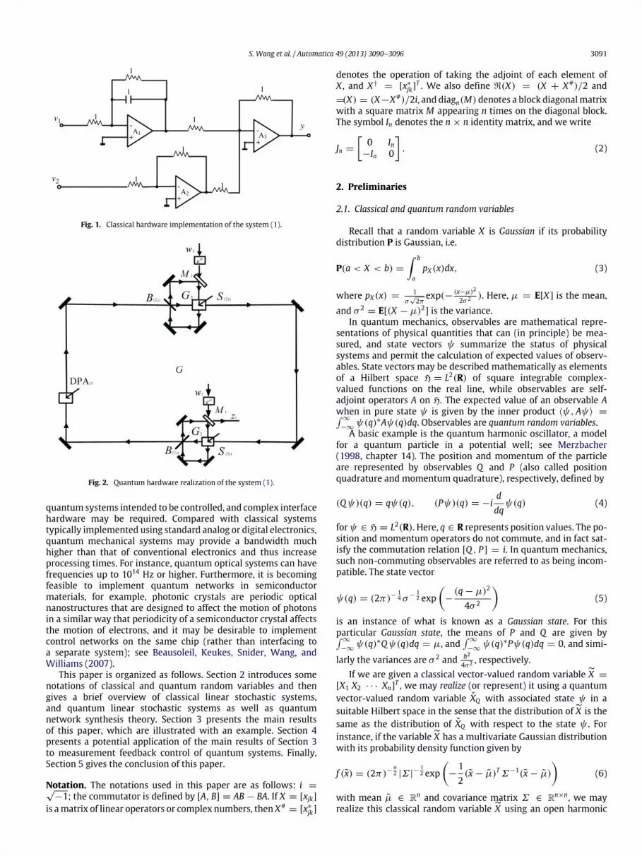
With the birth and development of quantum technologies,quantum control systems constructed using quantum optical de-vices play a more and more important role in control engineer-ing, Wiseman and Milburn (1993, 1994, 2009). Linear systems areof basic importance to control engineering, and also arise in themodeling and control of quantum systems; see Gardiner and Zoller(2004) andWiseman andMilburn (2009). A classical linear systemdescribed by the state space representation can be realized usingelectrical and electronic components by linear electrical networksynthesis theory, see Anderson and Vongpanitlerd (1973). For ex-ample, consider a classical system given bydξ(t) = −ξ(t)dt + dv1(t)dy(t) = ξ(t)dt + dv2(t) (1)where ξ(t) is the state, v1(t) and v2(t) are two independentstandardWiener processes, and y(t) is the output. Implementation

✩ The work was supported by AFOSR Grants FA2386-09-1-4089 and FA2386-12-1-4075, and theAustralianResearchCouncil. Thematerial in this paperwas partiallypresented at the Australian Control Conference (AUCC), November 10–11, 2011,Melbourne, Australia. This paper was recommended for publication in revised formby Associate Editor George Yin under the direction of Editor Ian R. Petersen.

E-mail addresses: shi.wang@anu.edu.au (S. Wang), h.nurdin@unsw.edu.au(H.I. Nurdin), Guofeng.Zhang@polyu.edu.hk (G. Zhang),Matthew.James@anu.edu.au (M.R. James).1 Tel.: +61 261258826; fax: +61 261250506.

0005-1098/$ – see front matter© 2013 Elsevier Ltd. All rights reserved.http://dx.doi.org/10.1016/j.automatica.2013.07.014

of the system (1) at the hardware level is shown in Fig. 1.Analogously to the electrical network synthesis theory of how tosynthesize linear analog circuits from basic electrical components,Nurdin, James, and Doherty (2009) have proposed a quantumnetwork synthesis theory (briefly introduced in Section 2.4 of thispaper), which details how to realize a quantum system describedby state space representations using quantum optical devices.

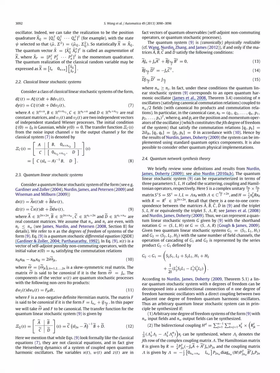
The purpose of this paper is to address this issue of quantumphysical realization for a class of classical linear stochastic systems.For example, the quantum physical realization of the system (1)is shown in Fig. 2 (see Example 1 in Section 3 for more details).The essential quantum optical components used in Fig. 2 includeoptical cavities, degenerate parametric amplifiers (DPA), phaseshifters, beam splitters, squeezers, etc.; interested readers mayrefer to Bachor and Ralph (2004) and Nurdin, James, Doherty(2009) for a more detailed introduction to these optical devices.The problem of quantum physical realization can be solved byembedding the classical system into a larger linear quantumsystem, Theorem 1. In this way, the classical system is representedas an invariant commutative subsystem of the larger quantumsystem.

While the results of this paper may be useful for a variety ofproblems outside the scope of measurement feedback control, theprincipal motivation for realizing classical systems in quantumhardware is that one is better able to match the timescalesand hardware of a classical controller to the system beingcontrolled. Classical hardware is typically much slower than the

S. Wang et al. / Automatica 49 (2013) 3090–3096 3091

Fig. 1. Classical hardware implementation of the system (1).

Fig. 2. Quantum hardware realization of the system (1).

quantum systems intended to be controlled, and complex interfacehardware may be required. Compared with classical systemstypically implemented using standard analog or digital electronics,quantum mechanical systems may provide a bandwidth muchhigher than that of conventional electronics and thus increaseprocessing times. For instance, quantum optical systems can havefrequencies up to 1014 Hz or higher. Furthermore, it is becomingfeasible to implement quantum networks in semiconductormaterials, for example, photonic crystals are periodic opticalnanostructures that are designed to affect the motion of photonsin a similar way that periodicity of a semiconductor crystal affectsthe motion of electrons, and it may be desirable to implementcontrol networks on the same chip (rather than interfacing toa separate system); see Beausoleil, Keukes, Snider, Wang, andWilliams (2007).

This paper is organized as follows. Section 2 introduces somenotations of classical and quantum random variables and thengives a brief overview of classical linear stochastic systems,and quantum linear stochastic systems as well as quantumnetwork synthesis theory. Section 3 presents the main resultsof this paper, which are illustrated with an example. Section 4presents a potential application of the main results of Section 3to measurement feedback control of quantum systems. Finally,Section 5 gives the conclusion of this paper.

Notation. The notations used in this paper are as follows: i =√−1; the commutator is defined by [A, B] = AB − BA. If X = [xjk]

is amatrix of linear operators or complex numbers, then X#= [x∗

jk]

denotes the operation of taking the adjoint of each element ofX , and XĎ

= [x∗

jk]T . We also define ℜ(X) = (X + X#)/2 and

ℑ(X) = (X−X#)/2i, and diagn(M) denotes a block diagonalmatrixwith a square matrix M appearing n times on the diagonal block.The symbol In denotes the n × n identity matrix, and we write

Jn =

0 In

−In 0

. (2)

2. Preliminaries

2.1. Classical and quantum random variables

Recall that a random variable X is Gaussian if its probabilitydistribution P is Gaussian, i.e.

P(a < X < b) =

b

apX (x)dx, (3)

where pX (x) =1

σ√2π

exp(− (x−µ)2

2σ 2 ). Here, µ = E[X] is the mean,and σ 2

= E[(X − µ)2] is the variance.In quantum mechanics, observables are mathematical repre-

sentations of physical quantities that can (in principle) be mea-sured, and state vectors ψ summarize the status of physicalsystems and permit the calculation of expected values of observ-ables. State vectors may be described mathematically as elementsof a Hilbert space H = L2(R) of square integrable complex-valued functions on the real line, while observables are self-adjoint operators A on H. The expected value of an observable Awhen in pure state ψ is given by the inner product ⟨ψ, Aψ⟩ =

∞

−∞ψ(q)∗Aψ(q)dq. Observables are quantum random variables.

A basic example is the quantum harmonic oscillator, a modelfor a quantum particle in a potential well; see Merzbacher(1998, chapter 14). The position and momentum of the particleare represented by observables Q and P (also called positionquadrature and momentum quadrature), respectively, defined by

(Qψ)(q) = qψ(q), (Pψ)(q) = −iddqψ(q) (4)

forψ ∈ H = L2(R). Here, q ∈ R represents position values. The po-sition and momentum operators do not commute, and in fact sat-isfy the commutation relation [Q , P] = i. In quantum mechanics,such non-commuting observables are referred to as being incom-patible. The state vector

ψ(q) = (2π)−14 σ−

12 exp

−(q − µ)2

4σ 2

(5)

is an instance of what is known as a Gaussian state. For thisparticular Gaussian state, the means of P and Q are given by

∞

−∞ψ(q)∗Qψ(q)dq = µ, and

∞

−∞ψ(q)∗Pψ(q)dq = 0, and simi-

larly the variances are σ 2 and h2

4σ 2 , respectively.If we are given a classical vector-valued random variable X =

[X1 X2 · · · Xn]T , we may realize (or represent) it using a quantum

vector-valued random variable XQ with associated state ψ in asuitable Hilbert space in the sense that the distribution ofX is thesame as the distribution of XQ with respect to the state ψ . Forinstance, if the variableX has a multivariate Gaussian distributionwith its probability density function given by

f (x) = (2π)−n2 |Σ |

−12 exp

−

12(x − µ)TΣ−1(x − µ)

(6)

with mean µ ∈ Rn and covariance matrix Σ ∈ Rn×n, we mayrealize this classical random variable X using an open harmonic

3092 S. Wang et al. / Automatica 49 (2013) 3090–3096

oscillator. Indeed, we can take the realization to be the positionquadrature XQ = [Q T

1 Q T2 · · · Q T

n ]T (for example), with the state

ψ selected so that (µ,Σ2) = (µQ ,Σ2Q ). So statistically X ≡ XQ .

The quantum vector X = [XTQ XT

P ]T is called an augmentation ofX , where XP = [PT

1 PT2 · · · PT

n ]T is the momentum quadrature.

The quantum realization of the classical random variable may be

expressed asX ≡In 0n×n

XQXP

.

2.2. Classical linear stochastic systems

Consider a class of classical linear stochastic systems of the form,

dξ(t) = Aξ(t)dt + Bdv1(t),dy(t) = Cξ(t)dt + Ddv2(t), (7)

where A ∈ Rn×n, B ∈ Rn×nv1 , C ∈ Rny×n and D ∈ Rny×nv2 are realconstantmatrices, and v1(t) and v2(t) are two independent vectorsof independent standard Wiener processes. The initial conditionξ(0) = ξ0 is Gaussian, while y(0) = 0. The transfer functionΞC (s)from the noise input channel v to the output channel y for theclassical system (7) is denoted by

ΞC (s) =

A

B, 0n×nv2

C

0nv2×nv2

, D

(s)

=

C (sIn − A)−1 B, D. (8)

2.3. Quantum linear stochastic systems

Consider a quantum linear stochastic systemof the form (see e.g.Gardiner and Zoller (2004), Nurdin, James, and Petersen (2009) andWiseman and Milburn (2009))

dx(t) = Ax(t)dt +Bdw(t),dz(t) = Cx(t)dt +Ddw(t), (9)

whereA ∈ R2n×2n,B ∈ R2n×nw , C ∈ Rnz×2n and D ∈ Rnz×nw arereal constant matrices. We assume that nw and nz are even, withnz ≤ nw (see James, Nurdin, and Petersen (2008, Section II) fordetails). We refer to n as the degrees of freedom of systems of theform (9). Eq. (9) is a quantum stochastic differential equation (QSDE)(Gardiner & Zoller, 2004; Parthasarathy, 1992). In Eq. (9), x(t) is avector of self-adjoint possibly non-commuting operators, with theinitial value x(0) = x0 satisfying the commutation relations

x0jx0k − x0kx0j = 2iΘjk, (10)

where Θ = [Θjk]j,k=1,2,...,2n is a skew-symmetric real matrix. Thematrix Θ is said to be canonical if it is the form Θ = Jn. Thecomponents of the vector w(t) are quantum stochastic processeswith the following non-zero Ito products:

dwj(t)dwk(t) = Fjkdt, (11)

where F is a non-negative definite Hermitian matrix. The matrix Fis said to be canonical if it is the form F = Inw + iJ nw

2. In this paper

we will take Θ and F to be canonical. The transfer function for thequantum linear stochastic system (9) is given by

ΞQ (s) =

A BC D(s) = C

sI2n −A−1B +D. (12)

Here wemention that while Eqs. (9) look formally like the classicalequations (7), they are not classical equations, and in fact givethe Heisenberg dynamics of a system of coupled open quantumharmonic oscillators. The variables x(t), w(t) and z(t) are in

fact vectors of quantum observables (self-adjoint non-commutingoperators, or quantum stochastic processes).

The quantum system (9) is (canonically) physically realizable(cf. Wang, Nurdin, Zhang, and James (2012)), if and only if the ma-tricesA,B,C andD satisfy the following conditions:AJn + JnAT

+BJ nw2BT

= 0, (13)BJ nw2DT

= −JnCT , (14)DJ nw2DT

= J nz2

(15)

where nw ≥ nz . In fact, under these conditions the quantum lin-ear stochastic system (9) corresponds to an open quantum har-monic oscillator (James et al., 2008, Theorem 3.4) consisting of noscillators (satisfying canonical commutation relations) coupled tonw/2 fields (with canonical Ito products and commutation rela-tions). In particular, in the canonical case, x0 = (q1, q2, . . . , qn, p1,p2, . . . , pn)T , where qj and pj are the position andmomentumoper-ators of the oscillator j (which constitutes the jth degree of freedomof the system) that satisfy the commutation relations [qj, pk] =

2iδjk, [qj, qk] = [pj, pk] = 0 in accordance with (10). Hence bythe results of Nurdin, James, Doherty (2009) the system can be im-plemented using standard quantum optics components. It is alsopossible to consider other quantum physical implementations.

2.4. Quantum network synthesis theory

We briefly review some definitions and results from Nurdin,James, Doherty (2009); see also Nurdin (2010a,b). The quantumlinear stochastic system (9) can be reparameterized in terms ofthree parameters S, L,H called the scattering, coupling and Hamil-tonian operators, respectively. Here S is a complex unitary nw

2 ×nw2

matrix SĎS = SSĎ = I , L = Λx0 withΛ ∈ Cnw2 ×2n, andH =

12x

T0Rx0

with R = RT∈ R2n×2n. Recall that there is a one-to-one corre-

spondence between the matrices A, B, C, D in (9) and the tripletS, L,H or equivalently the triplet S,Λ, R; see James et al. (2008)and Nurdin, James, Doherty (2009). Thus, we can represent a quan-tum linear stochastic system G given by (9) with the shorthandnotation G = (S, L,H) or G = (S,Λ, R) (Gough & James, 2009).Given two quantum linear stochastic systems G1 = (S1, L1,H1)and G2 = (S2, L2,H2)with the same number of field channels, theoperation of cascading of G1 and G2 is represented by the seriesproduct G2 ▹ G1 defined by

G2 ▹ G1 =

S2S1, L2 + S2L1,H1 + H2

+12i(LĎ2S2L1 − LĎ1S

Ď2L2)

.

According to Nurdin, James, Doherty (2009, Theorem 5.1) a lin-ear quantum stochastic system with n degrees of freedom can bedecomposed into a unidirectional connection of n one degree offreedom harmonic oscillators with a direct coupling between twoadjacent one degree of freedom quantum harmonic oscillators.Thus an arbitrary quantum linear stochastic system can in prin-ciple be synthesized if:

(1) Arbitrary one degree of freedomsystems of the form (9)withnw input fields and nw output fields can be synthesized.

(2) The bidirectional coupling Hd=

n−1j=1

nk=j+1 x

Tk ×

RTjk −

12i (Λ

ĎkΛj − ΛT

kΛ#j )

xj can be synthesized, where Λj denotes the

jth row of the complex couplingmatrixΛ. The HamiltonianmatrixR is given by R =

14P

T2n(−JnA + AT Jn)P2n and the coupling matrix

Λ is given by Λ = −i2

0nw×nw Inw

P2nwdiagnw (M)P

T2nw

BT JnP2n

S. Wang et al. / Automatica 49 (2013) 3090–3096 3093

Fig. 3. Quantum realization of classical systemΞC : v → y.

where M =

1 −i1 i

, and P2n denotes a permutation matrix acting

on a column vector f = [f1 f2 · · · f2n]T as P2nf = [f1 f1+n f2 f2+n· · · fn f2n]T .

The work Nurdin, James, Doherty (2009) then shows howone degree of freedom systems and the coupling Hd can beapproximately implemented using certain linear and nonlinearquantum optical components. Thus in principle any system of theform (9) can be constructed using these components. In Section 3we will use the construction proposed in Nurdin, James, Doherty(2009) to realize systems of the form (9)without further comment.The details of the construction and the individual componentsinvolved can be found in Nurdin, James, Doherty (2009) and thereferences therein.

3. Quantum physical realization

In this section we present our results concerning the quantumphysical realization of classical linear stochastic systems and thenprovide an example to illustrate the results. As is well known, for alinear system, its state space representation can be associated to aunique transfer function representation. Then, we will show howthe transfer function matrixΞC (s) can be realized (in a sense to bedefined more precisely below) using linear quantum components.In general, the dimension of vectors in (9) is greater than the vectordimension in (7), and so to obtain a quantum realization of theclassical system (7) using the quantum system (9) we require thatthe transfer functions be related by

ΞC (s) = MoΞQ (s)Mi, (16)

as illustrated in Fig. 3. Here, the matrix Mi and Mo correspondto operation of selecting elements of the input vector w(t) andthe output vector z(t) of the quantum realization that correspondto quantum representation of v(t) and y(t), respectively (asdiscussed in Section 2). In Fig. 3, the unlabeled box on the leftindicates that v(t) is represented as some subvector of w(t) (e.g.modulation2), whereas the unlabeled box on the right indicatesthat y(t) corresponds to some subvector of z(t) (quadraturemeasurement).

Definition 1. The classical linear stochastic system (7) is said tobe canonically realized by the quantum linear stochastic system (9)provided:

(1) The dimension of the quantum vectors x(t), w(t) and z(t) aretwice the lengths of the corresponding classical vectors x(t),v(t) = [v1(t)T v2(t)T ]T and y(t), where x(t) = [ξ(t)T θ(t)T ]Twith ξ(t) = [q1(t) q2(t) · · · qn(t)]T and θ(t) = [p1(t) p2(t)· · · pn(t)]T , w(t) = [v1(t)T v2(t)T u1(t)T u2(t)T ]T and z(t) =

[y(t)T y′(t)T ]T .

2 Modulation is the process of merging two signals to form a third signal withdesirable characteristics of both in a manner suitable for transmission.

(2) The classical ΞC (s) and quantum ΞQ (s) transfer functions arerelated by Eq. (16) for the choice

Mo =Iny 0ny×ny

, Mi =

Inv 0nv×nv

T.

(3) The quantum linear stochastic system (9) is canonically phys-ically realizable (as described in Section 2.3) with the systemmatrices A, B, C andD having the special structure:

A =

A0 0n×nA1 A2

,

B =

B0 0n×nv2

0n×nv10n×nv2

B1 B2 B3 B4

,

C =

C0 0nw×nC1 C2

,

D =

0ny×nv1

D0 0ny×nv10ny×nv2

D1 D2 D3 D4

(17)

with A0 ∈ Rn×n, A1 ∈ Rn×n, A2 ∈ Rn×n, B0 ∈ Rn×nv1 ,B1 ∈ Rn×nv1 , B2 ∈ Rn×nv2 , B3 ∈ Rn×nv1 , B4 ∈ Rn×nv2 , C0 ∈

Rny×n, C1 ∈ Rny×n, C2 ∈ Rny×n, D0 ∈ Rny×nv2 , D1 ∈ Rny×nv1 ,D2 ∈ Rny×nv2 , D3 ∈ Rny×nv1 , and D4 ∈ Rny×nv2 .

Remark 1. According to the structure of the matrices A, B, C ,and D, and since the system (9) is physically realizable, it can beverified directly that commutation relations for ξ(t), θ(t) satisfy[ξ(t), ξ(s)T ] = 0, [ξ(t), θ(s)T ] = 0 and [θ(t), θ(s)T ] = 0 for allt, s ≥ 0. The quantum realization of the classical variable ξ(t)maybe expressed as ξ(t) =

I 0

x(t) =

I 0

ξ(t)θ(t)

. The structures

of thematrices A, B, C andD in the above definition ensure that theclassical system (7) can be embedded as an invariant commutativesubsystem of the quantum system (9), as discussed in Gough andJames (2009), James et al. (2008) and Wang et al. (2012). Here,the classical variables and the classical signals are representedwithin an invariant commutative subspace of the full quantumfeedback system, and the additional quantum degrees of freedomintroduced in the quantum controller have no influence on thebehavior of the feedback system; see James et al. (2008) fordetails. In fact, D represents static Bogoliubov transformations orsymplectic transformations, which can be realized as a suitablestatic quantum optical network (e.g. ideal squeezers), Nurdin(2012) and Nurdin, James, Doherty (2009).

In what follows we restrict our attention to stable classicalsystems, since it may not be desirable to attempt to implementan unstable quantum system. By a stable quantum system (9)we mean that the A is Hurwitz. We will seek stable quantumrealizations. Furthermore, given the quantumphysical realizabilityconditions (13)–(15), we cannot do the quantum realizations foran arbitrary classical system (7). For these reasons we make thefollowing assumptions regarding the classical linear stochasticsystem (7).

Assumption 1. Assume the following conditions hold:

(1) The matrix A is a Hurwitz matrix.(2) The pair (−A, B) is stabilizable.(3) The matrix D is of full row rank.

Theorem 1. Under Assumption 1, there exists a stable quantumlinear stochastic system (9) realizing the given classical linearstochastic system (7) in the sense of Definition 1, where the matricesA, B, C and D can be constructed according to the following steps:

(1) A0 = A, B0 = B, C0 = C and D0 = D, with A B, C and D as givenin (7).

3094 S. Wang et al. / Automatica 49 (2013) 3090–3096

(2) B1, B2 are arbitrary matrices of suitable dimensions.(3) The matrices A2 and B3 can be fixed simultaneously by

A2 = −AT− B3BT (18)

where B3 is chosen to let A2 be a Hurwitz matrix.(4) The matrices B4 and D4 are given by

B4 = −CT (DDT )−1D + N1(D)T , (19)

D4 = (DDT )−1D + N2(D)T , (20)

where N1(D) (resp., N2(D)) denotes a matrix of the samedimension as BT

4 (resp., DT4) whose columns are in the kernel space

of D.(5) For a given D4, there always exist matrices D1,D2,D3 satisfying

− D3DT1 − D4DT

2 + D1DT3 + D2DT

4 = 0. (21)

The simplest choice is D1 = 0, D2 = 0, and D3 = 0.(6) The remaining matrices can be constructed as follows,

C2 = −D3BT (22)

C1 = D4BT2 + D3BT

1 − D2BT4 − D1BT

3 (23)

A1 = Ξ +12(B3BT

1 − B1BT3 − B2BT

4 + B4BT2) (24)

whereΞ is an arbitrary n × n real symmetric matrix.

Proof. The idea of the proof is to represent the classical stochasticprocesses ξ(t) and v(t) as quadratures of quantum stochasticprocesses x(t) and w(t) respectively, and then determine thematrices A, B, C and D in such a way that the requirements ofDefinition 1 and the Hurwitz property ofA are fulfilled. To this end,we set the number of oscillators to be n = nc , the number of fieldchannels as nw = 2nv = 2(nv1 + nv2) and the number of outputfield channels as nz = 2ny. Eqs. (18)–(24) can be obtained fromthe physical realizability constraints (13)–(15). According to thesecond assumption of Assumption 1, we can choose B3 such thatA2 = −AT

−B3BT is a Hurwitz matrix. From the first assumption ofAssumption 1, we can conclude thatA is a Hurwitz matrix, whichmeans the quantum linear stochastic system (9) is stable. UsingMiand Mo as defined in Definition 1 and then combining these withEqs. (17)–(24), we can verify the following relation between theclassicalΞC (s) and quantumΞQ (s) transfer functions,

MoΞQ (s)Mi =Iny 0ny×ny

×

C 0ny×nC1 C2

sI2n −

A 0n×nA1 A2

−1

×

B 0n×nv2

0n×nv10n×nv2

B1 B2 B3 B4

+D

×Inv 0nv×nv

T=

C 0ny×n

×

(sIn − A)−1 0n×n

(sIn − A2)−1A1(sIn − A)−1 (sIn − A2)

−1

×

B 0n×nv2B1 B2

+

0ny×nv1

D

=C (sIn − A)−1 B D

= ΞC (s).

This completes the proof. �

Example 1. Let us realize the classical system (1) introduced in

Section 1. The classical transfer function is ΞC (s) =

1

s + 11.

By Theorem 1, we can construct a quantum system G given by

dx1 = −x1dt + dv1dx2 = −x2dt + 2du1 − du2

dz1 = x1dt + dv2dz2 = du2. (25)

The quantum transfer function is given byΞQ (s) =

1

s + 11 0 0

0 0 0 1

.

Since in this case Mo =1 0

, Mi =

I2 02×2

T , we see thatΞC (s) = MoΞQ (s)Mi. The commutative subsystem dx1 = −x1dt +

dv1, dz1 = x1dt + dv2 can clearly be seen in these equations, withthe identifications y = z1, ξ = x1. It can be seen thatA,B,C andDsatisfy the physically realizable constraints (13) and (14).

Let us realize this classical system. The parameter R for G isgiven by R = 0, which means no Degenerate Parametric Amplifier(DPA) is required to implement R; see Nurdin, James, Doherty(2009, Section 6.1.2). The coupling matrixΛ for G is given by

Λ =

Λ1Λ2

=

−1 −0.5i0.5 0

.

From the above equation, we can get Λ1 = [−1 −0.5i] andΛ2 = [0.5 0]. The coupling operator L1 = Λ1x0 for G is given by

L1 = Λ1

qp

= Λ1

1 1−i i

aa∗

= −1.5a − 0.5a∗ (26)

where a =12 (q + ip) is the oscillator annihilation operator and

a∗=

12 (q−ip) is the creation operator of the systemGwithposition

andmomentum operators q and p, respectively. L1 can be approxi-mately realized by the combination of a two-mode squeezerΥG11 , abeam splitter BG12 , and an auxiliary cavity G1. If the dynamics of G1evolve on amuch faster time scale than that of G then the couplingoperator L1 is approximately given by: L1 =

1√γ1(−ϵ∗

12a + ϵ11a∗),where γ1 is the coupling coefficient of the only partially transmit-ting mirror of G1, ϵ11 is the effective pump intensity of ΥG11 andϵ12 is the coefficient of the effective Hamiltonian for BG12 given byϵ12 = 2Θ12e−iΦ12 , whereΘ12 is the mixing angle of BG12 andΦ12 isthe relative phase between the input fields introduced by BG12 ; seeNurdin, James, Doherty (2009). For this to be a good approximationwe require that

√γ1, |ϵ11|, |ϵ12| be sufficiently large, and assuming

that the coupling coefficient of the mirrorM1 is γ1 = 100, then wecan get ϵ11 = −5, ϵ12 = 15, Φ12 = 0 and Θ12 = 7.5. The scatter-ing matrix for G1 is eiπ = −1 and all other parameters are set to 0.In a similar way, the coupling operator L2 = Λ2x0 can be realizedby the combination of ΥG21 , BG22 , and G2. In this case, if we set thecoupling coefficient of the partially transmittingmirrorM2 of G2 toγ2 = 100, we find the effective pump intensity ϵ21 of ΥG21 givenby ϵ21 = 5, the relative phase Φ22 of BG22 given by Φ22 = π , themixing angle Θ22 of BG22 given by Θ22 = 2.5, and the scatteringmatrix for G2 to be eiπ = −1, with all other parameters set to 0.The implementation of the quantum system G is shown in Fig. 2.

4. Application

The main results of this paper may have a practical applicationin measurement feedback control of quantum systems, which isimportant in a number of areas of quantum technology, includ-ing quantum optical systems, nanomechanical systems, and circuitQED systems; seeWiseman andMilburn (1993, 2009). Inmeasure-ment feedback control, the plant is a quantum system, while thecontroller is a classical system (Wiseman & Milburn, 2009). Theclassical controller processes the outcomes of ameasurement of an

S. Wang et al. / Automatica 49 (2013) 3090–3096 3095

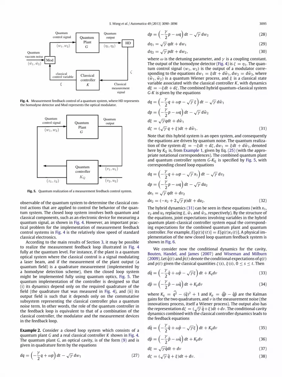
Fig. 4. Measurement feedback control of a quantum system, where HD representsthe homodyne detector and Mod represents the optical modulator.

Fig. 5. Quantum realization of a measurement feedback control system.

observable of the quantum system to determine the classical con-trol actions that are applied to control the behavior of the quan-tum system. The closed loop system involves both quantum andclassical components, such as an electronic device for measuring aquantum signal, as shown in Fig. 4. However, an important prac-tical problem for the implementation of measurement feedbackcontrol systems in Fig. 4 is the relatively slow speed of standardclassical electronics.

According to the main results of Section 3, it may be possibleto realize the measurement feedback loop illustrated in Fig. 4fully at the quantum level. For instance, if the plant is a quantumoptical system where the classical control is a signal modulatinga laser beam, and if the measurement of the plant output (aquantum field) is a quadrature measurement (implemented bya homodyne detection scheme), then the closed loop systemmight be implemented fully using quantum optics, Fig. 5. Thequantum implementation of the controller is designed so that(i) its dynamics depend only on the required quadrature of thefield (the quadrature that was measured in Fig. 4), and (ii) itsoutput field is such that it depends only on the commutativesubsystem representing the classical controller plus a quantumnoise term. In other words, the role of the quantum controller inthe feedback loop is equivalent to that of a combination of theclassical controller, the modulator and the measurement devicesin the feedback loop.

Example 2. Consider a closed loop system which consists of aquantum plant G and a real classical controller K shown in Fig. 4.The quantum plant G, an optical cavity, is of the form (9) and isgiven in quadrature form by the equations

dq =

−γ

2q + ωp

dt −

√γ dw1 (27)

dp =

−γ

2p − ωq

dt −

√γ dw2 (28)

dη1 =√γ qdt + dw1 (29)

dη2 =√γ pdt + dw2, (30)

where ω is the detuning parameter, and γ is a coupling constant.The output of the homodyne detector (Fig. 4) is ζ = η1. The quan-tum control signal (w1, w2) is the output of a modulator corre-sponding to the equations dw1 = ξdt + dw1, dw2 = dw2, where(w1, w2) is a quantum Wiener process, and ξ is a classical statevariable associated with the classical controller K , with dynamicsdξ = −ξdt + dζ . The combined hybrid quantum–classical systemG-K is given by the equations

dq =

−γ

2q + ωp −

√γ ξ

dt −

√γ dw1

dp =

−γ

2p − ωq

dt −

√γ dw2

dξ =√γ qdt + dw1

dζ = (√γ q + ξ)dt + dw1. (31)

Note that this hybrid system is an open system, and consequentlythe equations are driven by quantum noise. The quantum realiza-tion of the system dξ = −ξdt + dζ , dw1 = ξdt + dw1, denotedhere by KQ is, from Example 1, given by Eq. (25) (with the appro-priate notational correspondences). The combined quantum plantand quantum controller system G-KQ is specified by Fig. 5, withcorresponding closed loop equations

dq =

−γ

2q + ωp −

√γ x1

dt −

√γ dv2

dp =

−γ

2p − ωq

dt −

√γ du2

dx1 =√γ qdt + dv2

dx2 = (−x2 + 2√γ p)dt + du2. (32)

The hybrid dynamics (31) can be seen in these equations (with x1,v2 and u2 replacing ξ , w1 and w2, respectively). By the structure ofthe equations, joint expectations involving variables in the hybridquantum plant–classical controller system equal the correspond-ing expectations for the combined quantum plant and quantumcontroller. For example, E[q(t)ξ(t)] = E[q(t)x1(t)]. A physical im-plementation of the new closed loop quantum feedback system isshown in Fig. 6.

We consider now the conditional dynamics for the cavity,Bouten, Handel, and James (2007) and Wiseman and Milburn(2009). Let q(t) and p(t)denote the conditional expectations of q(t)and p(t) given the classical quantities ζ (s), ξ(s), 0 ≤ s ≤ t . Then

dq =

−γ

2q + ωp −

√γ ξ

dt + Kqdν (33)

dp =

−γ

2p − ωq

dt + Kpdν (34)

where Kq = q2 − (q)2 + 1 and Kp = qp − qp are the Kalmangains for the two quadratures, and ν is themeasurement noise (theinnovations process, itself a Wiener process). The output also hasthe representation dζ = (

√γ q+ξ)dt+dν. The conditional cavity

dynamics combinedwith the classical controller dynamics leads tothe feedback equations

dq =

−γ

2q + ωp −

√γ ξ

dt + Kqdν (35)

dp =

−γ

2p − ωq

dt + Kpdν (36)

dξ =√γ qdt + dν (37)

dζ = (√γ q + ξ)dt + dν. (38)

3096 S. Wang et al. / Automatica 49 (2013) 3090–3096

Fig. 6. Quantum realization of the closed-loop system shown in Fig. 5.

Here we can see the measurement noise ν(t) explicitly in thefeedback equations. By properties of conditional expectation, wecan relate expectations involving the conditional closed loop sys-tem with the hybrid quantum plant–classical controller system,e.g. E[q(t)ξ(t)] = E[q(t)ξ(t)]. We therefore see that the expec-tations involving the hybrid system, the conditional system, andthe quantum plant–quantum controller system are all consistent.

5. Conclusion

In this paper, we have shown that a class of classical linearstochastic systems (having a certain form and satisfying certaintechnical assumptions) can be realized by quantum linear stochas-tic systems. It is anticipated that the main results of the workwill aid in facilitation of the implementation of classical linearstochastic systems with fast quantum optical devices (e.g. mea-surement feedback control), especially inminiature platforms suchas nanophotonic circuits.

References

Anderson, B. D. O., & Vongpanitlerd, S. (1973). Networks series, Network analysis andsynthesis: amodern systems theory approach. EnglewoodCliffs, NJ: Prentice-Hall.

Bachor, H. A., & Ralph, T. C. (2004). A guide to experiments in quantum optics (2nded.). Weinheim, Germany: Wiley-VCH.

Beausoleil, R. G., Keukes, P. J., Snider, G. S., Wang, S., & Williams, R. S. (2007).Nanoelectronic and nanophotonic interconnect. Proceedings of the IEEE, 96,230–247.

Bouten, L., Handel, R. V., & James,M. R. (2007). An introduction to quantum filtering.SIAM Journal on Control and Optimization, 46(6), 2199–2241.

Gardiner, C., & Zoller, P. (2004). Quantum noise (3rd ed.). Berlin, Germany: Springer.Gough, J. E., & James,M. R. (2009). The series product and its application to quantum

feedforward and feedback networks. IEEE Transactions on Automatic Control,54(11), 2530–2544.

James, M. R., Nurdin, H. I., & Petersen, I. R. (2008). H∞ control of linear quantumstochastic systems. IEEE Transactions on Automatic Control, 53, 1787–1803.

Merzbacher, E. (1998). Quantum mechanics (3rd ed.). New York: Wiley.Nurdin, H. I. (2010a). Synthesis of linear quantum stochastic systems via quantum

feedback networks. IEEE Transactions on Automatic Control, 55(4), 1008–1013.Extended preprint version available at http://arxiv.org/abs/0905.0802.

Nurdin, H. I. (2010b). On synthesis of linear quantum stochastic systems by purecascading. IEEE Transactions on Automatic Control, 55(10), 2439–2444.

Nurdin, H.I. (2012). Network synthesis of mixed quantum–classical linear stochas-tic systems. In Proceedings of the 2011 Australian control conference (AUCC),Engineers Australia. Australia (pp. 68–75).

Nurdin, H. I., James, M. R., & Doherty, A. C. (2009). Network synthesis oflinear dynamical quantum stochastic systems. SIAM Journal on Control andOptimization, 48, 2686–2718.

Nurdin, H. I., James, M. R., & Petersen, I. R. (2009). Coherent quantum LQG control.Automatica, 45, 1837–1846.

Parthasarathy, K. (1992). An introduction to quantum stochastic calculus. Berlin,Germany: Birkhauser.

Wang, S., Nurdin, H.I., Zhang, G., & James, R.M. (2012). Synthesis and structureof mixed quantum–classical linear systems. In Proceedings of the 51st IEEEconference on decision and control, CDC. (pp. 1093–1098).

Wiseman, H. M., & Milburn, G. J. (1993). Quantum theory of optical feedback viahomodyne detection. Physical Review Letters, 70, 548–551.

Wiseman, H.M., &Milburn, G. J. (1994). All-optical versus electro-optical quantum-limited feedback. Physics Review A, 49(5), 4110–4125.

Wiseman, H. M., & Milburn, G. J. (2009). Quantum measurement and control.Cambridge, UK: Cambridge University Press.

Shi Wang received his Master’s degree from Northeast-ern University, Shenyang, China, in 2008. Now he is a Ph.Dcandidate under the supervision of Professor Matthew R.James at the Australian National University, Australia. Hiscurrent research interests include quantumcoherent feed-back control, quantum network analysis and synthesis.

Hendra I. Nurdin received a Bachelor’s degree in electricalengineering from Institut Teknologi Bandung, Indonesia, aMaster’s degree in engineeringmathematics from the Uni-versity of Twente, The Netherlands, and a Ph.D. degree inengineering and information science from the AustralianNational University, Australia, in 2007. After receiving hisPh.D. he remained at ANU for four more years where hewas a Research Fellow in the Department of Engineering(2007–2008) and then an Australian Research Council APDFellow in the School of Engineering (2009–2011).

He joined the School of Electrical Engineering andTelecommunications at the University of New SouthWales (UNSW) in Sydney, Aus-tralia, in 2012 where he is currently a senior lecturer. His broad research interest isin the area of systems and control theory, and particular interests include stochas-tic modeling, stochastic systems and control, and quantum control. Dr Nurdin is aSenior Member of the IEEE.

Guofeng Zhang received the B.Sc and M.Sc. degrees fromNortheastern University, Shenyang, China, in 1998 and2000, respectively, and the Ph.D. degree in applied math-ematics from the University of Alberta, Edmonton, AB,Canada, in 2005.

During 2005–2006, he was a Postdoc Fellow in the De-partment of Electrical and Computer Engineering, Univer-sity ofWindsor,Windsor, ON, Canada. He joined the Schoolof Electronic Engineering, University of Electronic Scienceand Technology of China, Chengdu, Sichuan, in 2007. He iscurrently an Assistant Professor in the Department of Ap-

plied Mathematics, The Hong Kong Polytechnic University, Hong Kong, China. Hisresearch interests include quantum control, sampled-data control and nonlineardynamics.

Matthew R. James was born in Sydney, Australia, in1960. He received the B.Sc. degree in mathematics andthe B.E. (Hon. I) in electrical engineering from theUniversity of New SouthWales, Sydney, Australia, in 1981and 1983, respectively. He received the Ph.D. degree inapplied mathematics from the University of Maryland,College Park, USA, in 1988. In 1988/1989 Dr James wasVisiting Assistant Professor with the Division of AppliedMathematics, Brown University, Providence, USA, andfrom 1989 to 1991 he was Assistant Professor withthe Department of Mathematics, University of Kentucky,

Lexington, USA.In 1991 he joined the Australian National University, Australia, where he served

as Head of the Department of Engineering during 2001 and 2002. He has heldvisiting positions with the University of California, San Diego, Imperial College,London, and the University of Cambridge. His research interests include quantum,nonlinear, and stochastic control systems.

Dr James is a co-recipient (with Drs L. Bouten and R. Van Handel) of theSIAM Journal on Control and Optimization Best Paper Prize for 2007. He iscurrently serving as Associate Editor for EPJ Quantum Technology and AppliedMathematics and Optimization, and has previously served as Associate Editor forIEEE Transactions on Automatic Control, SIAM Journal on Control and Optimization,Automatica, and Mathematics of Control, Signals, and Systems. He is a Fellow ofthe IEEE, and held an Australian Research Council Professorial Fellowship during2004–2008.