arX

iv:1

305.

6981

v3 [

phys

ics.

com

p-ph

] 2

6 Ju

n 20

13

Linear-scaling and parallelizable algorithms for stochastic quantum chemistry

George H. Booth1,2,∗ Simon D. Smart1, and Ali Alavi1

Chemistry Department, University of Cambridge, Lensfield Road, Cambridge CB2 1EW, UK and

Department of Chemistry, Frick Laboratory, Princeton University, NJ 08544, USA

(Dated: June 27, 2013)

For many decades, quantum chemical method development has been dominated by algorithmswhich involve increasingly complex series of tensor contractions over one-electron orbital spaces.Procedures for their derivation and implementation have evolved to require the minimum amountof logic and rely heavily on computationally efficient library-based matrix algebra and optimizedpaging schemes. In this regard, the recent development of exact stochastic quantum chemicalalgorithms to reduce computational scaling and memory overhead requires a contrasting algorithmicphilosophy, but one which when implemented efficiently can often achieve higher accuracy/costratios with small random errors. Additionally, they can exploit the continuing trend for massiveparallelization which hinders the progress of deterministic high-level quantum chemical algorithms.In the Quantum Monte Carlo community, stochastic algorithms are ubiquitous but the discrete Fockspace of quantum chemical methods is often unfamiliar, and the methods introduce new conceptsrequired for algorithmic efficiency. In this paper, we explore these concepts and detail an algorithmused for Full Configuration Interaction Quantum Monte Carlo (FCIQMC), which is implementedand available in MOLPRO and as a standalone code, and is designed for high-level parallelism andlinear-scaling with walker number. Many of the algorithms are also in use in, or can be transferredto, other stochastic quantum chemical methods and implementations. We apply these algorithmsto the strongly correlated Chromium dimer, to demonstrate their efficiency and parallelism.

I. INTRODUCTION

Post Hartree–Fock methods encompass a range of toolsto account for electronic correlations within quantumchemical calculations. Such methods are required toprogress from a (generally) qualitative description of asystem at the Hartree–Fock level and approach quantita-tive agreement with experimental results[1]. Recently,three of the most commonly-used methods have beenrecast in a formalism amenable to stochastic evalua-tion. Each of these has been found to have a num-ber of advantages over their deterministic counterparts,underlining the potential of these methods. Stochas-tic versions of Configuration Interaction (FCIQMC)[2–4], Coupled-Cluster (CCMC)[5], and Møller–Plesset per-turbation theory[6] can benefit from reduced computa-tional effort compared to their deterministic counter-parts, while faithfully reproducing the same results, al-beit with small and systematically controllable randomerrors, thus maintaining the hallmark of reproducibilityin quantum chemical methods. The stochastic meth-ods discussed here differ from other recent quantumchemical Monte Carlo schemes based on direct energyevaluation[7–10], as here the wavefunctions are sampledand optimized in the space of orthogonal Slater determi-nants.

It may seem counter-intuitive that improvements canbe found by removing the large linear algebra routinesthat are so suited to fast computation, but the returncomes from the fact that while quantum chemical Hilbert

∗Electronic address: ghb24@cam.ac.uk

spaces are so large, their internal connectivity is relativelysmall, and there is generally significant sparsity in boththe Hamiltonian and the wavefunction[11]. In traditionalformulations, deterministic evaluation results in equalcomputational effort in realizing each determinant andtransition in the space, regardless of amplitude[1, 12, 13].In stochastic analogues low-weighted functions in thespace, with few ‘walkers’ residing on them and smalltransition probabilites leading to them, consume littlecomputation effort. Since the low-weighted amplitudesare rarely sampled, each instantaneous snapshot of thewalker ensemble represents a coarse-grained, and highlycompressed representation of the wavefunction, with onlysmall parts of the space instantaneously occupied[14].Therefore, the sparsity in the wavefunction can be re-flected in the size of the instantaneous walker distribu-tion, lifting the burden of wavefunction storage which isgenerally the bottleneck in exact diagonalization (FCI)methods[13, 15]. Nevertheless, time averaging over theseinstantaneous snapshots within an appropriate dynamiccan correctly reproduce the wavefunction and energy es-timators.It should be noted that deterministic schemes to ex-

ploit the sparsity in both the many- and one-electronspaces is a source of much research in wavefunction-basedelectronic structure theory. For example, where the or-bitals can be localized, cutoffs and local domains are pro-viding a route to take advantage of the generally short-range nature of correlation and to minimize the redun-dancy in the space[16–19]. Additionally, tensor factoriza-tions of the wavefunction amplitudes aim for an alterna-tive compression of the wavefunction complexity[20–24].It is an unresolved and interesting question as to whetherthe stochastic methods could similarly benefit from suchlocalization of the Fock space or tensor network structure

2

imposed on the amplitudes.Within these stochastic methods, close control over

the sampled Hamiltonian gives rise to additional pos-sibilities. Since Hamiltonian matrix elements are sam-pled individually, small dynamic modifications and addi-tional criteria on the many-body space can give rise toa number of systematically improvable approximations,which can be difficult or impossible to impose in deter-ministic methods[14, 25–28]. This approach can againdramatically reduce the computational effort needed toconverge to the solution. In addition to this, stochasticmethods can also benefit from improved parallelizationover distributed memory machines, an important trait onmodern computer architecture, and one which high-levelquantum chemical algorithms can particularly strugglewith[29]. The efficiency of this parallelism will be ex-plored in this paper.In this paper, we focus on the original ‘initiator’

i-FCIQMC algorithm. This method has proven success-ful in providing exact basis-set energies of systems welloutside the limit of what can be achieved within iter-ative diagonalization schemes in a variety of differentsystems[14, 27, 30–32]. By reformulating the underly-ing dynamic of the walker distribution, advances in thescope of the method have also been achieved. Com-plex wavefunctions[30], excited states[33], multi-statesolutions[34, 35] and finite temperature[36], as well asother techniques to reduce the random error or scalingwith system size[37, 38] have been developed. In addi-tion, advances in parent deterministic methods can oftenbe transferred to their stochastic counterparts, with ex-plicitly correlated versions of the theory and density ma-trices able to be sampled[39, 40]. Many of these meth-ods can be considered as modifications to the underlyingwalker dynamics of the FCIQMC algorithm from an im-plementational point of view, and so will hopefully alsobenefit from the careful consideration of this algorithmhere. We shall analyze the performance and implementa-tion of the algorithms which are so critical to the method,before resolving the electronic effects of the chromiumdimer, a molecular system exhibiting non-trivial stronglycorrelated wavefunction structure.

II. OVERVIEW OF THE FCIQMC ALGORITHM

The key dynamical equations of FCIQMC that are es-sential to describe the algorithm are detailed here, but amore complete motivation and derivation can be foundelsewhere[2, 27]. The master equation which governs theevolution of the walker population is given by

C(n+1)i = [1− τ(Hii − E0 − S)]C

(n)i − τ

∑

j6=i

HijC(n)j .

(1)This equation can be derived from a finite-difference for-mulation of the imaginary-time Schrodinger equation,where the Hamiltonian, H , is projected into a discrete,

orthonormal N -electron basis |Di〉, constructed from aset of M one-electron orbitals. The ground-state wave-function in this basis is spanned by the coefficients Ci

after the master equation is iterated until convergenceat large n. The timestep, τ , represents the discretiza-tion of imaginary time, and S is a diagonal ‘shift’ whichis adjusted to maintain a constant number of walkers(L1-norm). At convergence, this can then be used as anestimate of the energy.An alternative single-reference ‘projected’ energy esti-

mator can be obtained from

E(n) =∑

i

〈Di|H |D0〉C(n)i

C(n)0

, (2)

where |D0〉 defines a reference determinant. This equa-tion is exact for the correct wavefunction distributionover the functions coupled to the reference, {|Di〉}, butthe random errors associated with this estimator are sen-sitive to the weight on this reference function. A multiref-erence reference function can be used, and allows for sys-tematic improvement over the single reference case[38].In the standard FCIQMC algorithm, the wavefunction

coefficients, Ci, are now discretized to an integer repre-sentation, where the value of this coefficient on a func-tion is denoted by the number of signed ‘walkers’ residingthere. This is not a unique representation of the wave-function coefficients. While some degree of discretizationis essential for the compression of the low-weighted am-plitudes, a multi-scale real/integer representation, wherea small region of importance is represented in a finer, con-tinuous, and deterministic fashion[38], has been found toprovide orders of magnitude saving in the random er-rors in many circumstances. This will not be consideredhere. In this paper, we will focus on the algorithm wherethe wavefunction representation, imaginary time, and off-diagonal dynamic are sampled and fully discretized, con-sistent with the majority of the literature to date.The dynamics of these walkers now follows a set of

steps designed to simulate the evolution of Eq. (1).First, for each walker on each determinant, |Di〉, asymmetry-allowed connected determinant, |Dj〉, is se-lected at random with a normalized and calculable proba-bility, Pgen(j|i). The spawning step of the algorithm thenproceeds by creating a new signed walker on |Dj〉 with astochastically realized probability[41] of

pspawn(j|i) = −sign(Ci)τHij

Pgen(j|i). (3)

Where this probability is negative, a particle with a neg-ative sign is created with probability |pspawn|. If thisprobability has magnitude larger than 1 then the corre-sponding integer number of particles are created deter-ministically, and the fractional part stochastically. Af-ter all walkers residing on determinant |Di〉 have beenthrough a spawning step, a local, diagonal death/cloningstep occurs. This step is applied to all walkers on thedeterminant at once, and reduces the population on the

3

local function with another stochastically realized prob-ability of

pdeath(i) = τCi(Hii − E0 − S). (4)

Where pdeath < 0 anti-particles are spawned which growthe population. As generally Hii ≥ E0 anti-particles areonly spawned for large, positive values of S. It shouldbe noted that walkers spawned, cloned or killed withinan iteration do not contribute to the subsequent steps ofthe same iteration.Taken together, these two steps simulate the dynam-

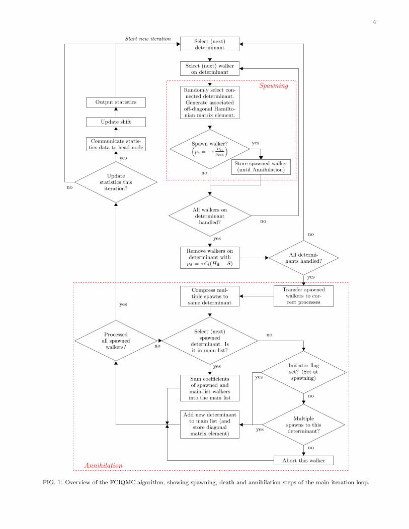
ics of Eq. (1). However, for general Fermionic wave-functions, it is impossible to find a representation of thewavefunction such that all Ci amplitudes are of the samesign[42]. This results in a propagation of both positiveand negative walkers, and a manifestation of the Fermionsign problem within this algorithm. Although this hasbeen shown in general to be less severe than the analo-gous problem within real-space QMC approaches[43], theFCIQMC algorithm can exactly overcome this exponen-tial reduction in signal to noise ratio via local annihi-lation events between oppositely signed walkers on thesame determinant[2, 44]. An important consequence forthis is that the walkers on each determinant at the be-ginning of an iteration are all of the same sign. It is alsoat this annihilation stage that additional approximationssuch as the successful ‘initiator’ adaptation of the methodcan be applied. The annihilation algorithm will be de-tailed in section IV. A flow diagram detailing the mainloop and logic structure of the overall algorithm is givenin Fig. 1.The innermost loops of the FCIQMC algorithm (the

spawning steps) involve random generation of symmetry-allowed connected determinants, and the calculation ofthe Hamiltonian matrix elements which connect the two.The generation of excitations is considered in section V,while the generation of matrix elements follows standardSlater–Condon rules (for a determinant basis)[1]. A sub-stantial cost in the algorithm, when using large basis sets,is memory latency in the one- and two–electron integrallookup between arbitrary orbitals required for these ma-trix elements. Since integrals are required in a randomorder, a pre-fetching algorithm to obtain multiple inte-grals at once is difficult to implement, while the O[M4]number of the integrals is likely to provide the mem-ory bottleneck in larger studies[63]. This is somewhatameliorated by a shared memory implementation (via ei-ther POSIX or System V shared memory[45, 46]), butfor large number of orbitals (& 250), either a density-fitted/Cholesky decomposed integral engine[47, 48] (toreduce integral storage to O[M3] or lower), on-the-flycalculation, distribution and communication of integralsbetween computational nodes or other compressed repre-sentation will likely be necessary. However, this will serveto increase the integral lookup cost and is not consideredfurther here. In all applications to date, the integralshave either been stored in memory on all computationalnodes, or calculated on-the-fly.

The other algorithmically and computationally non-trivial step required, which will be unfamiliar to stan-dard deterministic quantum chemistry packages and iskey to the performance of the method, is an efficient andscalable annihilation algorithm between walkers on thesame function with opposite sign. Much of the imple-mentation of the algorithm is with this in mind, sincenaive approaches can be very costly. This is also theonly step which involves communication between MPIthreads other than occasional aggregation of statistics,and is key to the parallel performance of the algorithm.It is important, therefore, to perform the MPI part ofthis step in a single, collective operation to reduce com-munication latency. The implementation of this step willbe considered in section IV.Unless such large numbers of parallel processes are

used that communication becomes the bottleneck, wehave found that excitation generation is the most costlypart of the algorithm. This is dependent on the numberof irreducible representations in the symmetry group be-ing used within the system (Nsym), as the cost increaseswith additional symmetry elements. However, we havefound it always worthwhile to make use of symmetrywhere possible, as this generally has a quadratic saving,since both the size and the internal connectivity of thespace are reduced by a factor of the number of symme-try elements, resulting in an increase in the p(j|i) valuesobtained in the spawning step and a corresponding in-crease in the timestep that can be used. Abelian sub-groups of D∞h are available, as are full Lz symmetries,translational point groups, total spin eigenfunctions andtime-reversal symmetries[27, 49, 50].Other factors such as the number of walkers, orbitals,

electrons and computational cores run on, as well as ef-fects such as the sparsity of the wavefunction will all in-fluence the efficiency of the algorithm and may changethe limiting step. The algorithm will generally becomeincreasingly parallelizable with increasing walker num-ber, as needed to converge the energy for larger systems.Because of this, we will focus on the computational ef-ficiency in the large walker limit of the algorithm, byoutlining a scheme for linear scaling with respect to thenumber of walkers, Nw, where availability of memory isnot a bottleneck. Derivatives of this scheme can be em-ployed in other computational regimes, where speed canbe sacrificed for memory saving, although these schemeswill not be discussed here as memory availability is gener-ally not the bottleneck of this algorithm on modern com-putational resources (as opposed to deterministic FCI).

III. REPRESENTATION OF WALKERS

The most simple N -electron space of the FCIQMC dy-namic is the complete set of Slater determinants, how-ever there are other function spaces which can span thesame Hilbert space, while being more compact. Theseinclude fixed combinations of determinants which obey

4

Select (next)determinant

Select (next) walkeron determinant

Randomly select con-nected determinant.Generate associatedoff-diagonal Hamilto-nian matrix element.

Spawn walker?(

ps = −τHij

pgen

)

Store spawned walker(until Annihilation)

All walkers ondeterminanthandled?

yes

no

Remove walkers ondeterminant withpd = τCi(Hii − S)

yes

All determi-nants handled?

Transfer spawnedwalkers to cor-rect processes

yes

Compress mul-tiple spawns to

same determinant

Select (next)spawned

determinant. Isit in main list?

Sum coefficientsof spawned andmain-list walkersinto the main list

yes Initiator flagset? (Set atspawning)

no

Multiplespawns to thisdeterminant?

no

Abort this walker

no

Add new determinantto main list (andstore diagonalmatrix element)

yes

yes

Processedall spawnedwalkers? no

Output statistics

Update shift

Communicate statis-tics data to head node

Updatestatistics thisiteration?

yes

yes

no

no

Start new iteration

no

Annihilation

Spawning

FIG. 1: Overview of the FCIQMC algorithm, showing spawning, death and annihilation steps of the main iteration loop.

5

spin-reversal symmetry (see section VC), momentum-reversal symmetry, or total spin eigenfunctions (configu-ration state functions[1]). Working in these other spacesinvolves a trade-off between the complexity of the exci-tation generation algorithms and matrix element evalu-ation, and the advantages provided by reductions in thetotal size and connectivity of the spaces, or when aimingseparately for ground and excited states which were pre-viously of the same symmetry. When ‘determinants’ arementioned here, it should be implicit that any of thesefunction spaces can be used in its place. Indeed, morecomplicated function spaces, including non-orthogonal orgeminal spaces may also provide interesting research di-rections in the future.

It is important for the FCIQMC algorithm that allof these functions can be uniquely and compactly repre-sented by bit strings indicating the occupations of the Morbitals (or 2M spin-orbitals) in the space. For deter-minants, this is straightforward and has been in use inprevious ‘string’-based schemes[13, 51]. For spin-coupledspaces, one unique determinant from the coupled pair ischosen to denote the function, so that the representa-tion is always the same. Many operations on determi-nants are then reduced to bit operations. For instance,finding the number of orbitals differing between two de-terminants can be computed via an ‘exclusive or’ oper-ation (XOR), followed by counting the set bits of theresult[52]. Additionally, checking whether two functionsare the same is equivalent to testing the equality of thebit-representations.

In our implementation, the bit-string is formulatedfrom an integer representation, and multiple integersare used when the number of spin-orbitals exceeds thenumber of bits in the integer type. In addition, an-other single integer is used to store the signed num-ber of walkers occupying the determinant, and any sin-gle bit ‘flags’ which may be required, such as whethera walker has been spawned from a function which isdeemed an ‘initiator’ (which confers special propertiesto the walker regarding its survival if spawned to an un-occupied determinant[26, 27]). To isolate the number ofwalkers on a determinant, their sign, or the associatedflag, separate masking integers are used to isolate thecomponent bits of this integer when desired via ANDoperations. This compression of multiple data into a sin-gle integer is done primarily to minimize the amount ofdata for communication purposes, rather than to save onmemory usage. For complex wavefunctions for use withcomplex irreducible representations such as translationalgroup symmetry and crystal momentum for solid-statesystems, or for other complex wavefunctions found in e.g.systems with spin-orbit coupling, two integers are usedfor the walker population to denote separately the realand imaginary parts of the wavefunction coefficient.

This representation of the walkers as a set of inte-gers uniquely denoting the determinant, signed numberof walkers, and any flags conferring special attributes isthe standard representation for all walkers in both the

main list, and the list for newly-spawned walkers each it-eration. The total number of 64-bit integers required tostore an occupied determinant in the main list thereforescales with number of orbitals as ⌈ 2M

64 ⌉ + 1. By way ofillustration, in a system with 128 spin-orbitals, 100Mbof memory will therefore store over four million occupieddeterminants, and assuming an optimal load-balancing(see section IV), this number of distinct occupied deter-minants can be stored on each computational process ondistributed memory architecture. It should be stressedthat the storage of the determinants is only ever per-formed over the instantaneously occupied determinants,and as such, no memory requirements which explicitlyscale with the size of the full Hilbert space are ever re-quired.Finally, it can be useful to store the diagonal Hamil-

tonian matrix elements for the occupied determinants inthe main list, along with the standard (integer) determi-nant representation. This is not essential, but saves onregeneration of these matrix elements, which involves anO[N2] operation, at each death step if a determinant re-mains occupied over multiple iterations. Crucially, thisdata does not need to be communicated in the annihi-lation step, and therefore involves only a memory costrather than increasing the quantity of data to communi-cate.

A. Encoding and Decoding of Determinant

Representations

Encoding of a newly occupied determinant bit-stringrepresentation from scratch is rarely required. Since de-terminants are generated through excitations of alreadyoccupied determinants, the bit representation of the newdeterminants may be calculated from the old in an O[1]step by clearing the bits representing the source orbitalsand setting those representing the targets. However, inthe excitation generation step, and for certain operationssuch as Hamiltonian matrix element calculation for singleexcitations and hashing (see section IV), an alternativedeterminant representation is preferable. In this ‘elec-tron occupation’ representation, an ordered set of N in-tegers are used to specify the spin-orbitals occupied byeach of the electrons in the function. This representationis generated for each occupied determinant from its bitrepresentation via a 1-to-1 ‘decoding’ function when it isconsidered in each iteration.Decoding can be performed naively by looping over all

the bits in the bit representation, and appending eachset bit to a list. However this is unnecessarily costly.In a similar way to one method of counting the num-ber of bits set in an integer[52], this may be approachedthrough subdividing the bit representation into individ-ual bytes, and creating a lookup table for the available256 possibilities[64]. Each possible byte has an entry con-taining i) the number of orbitals contained in this byte,and ii) a list of these orbitals (with the first bit in the byte

6

being orbital zero). Looping over all non-zero bytes, untilthe correct number of orbitals are found, is substantiallymore efficient than looping over each of the bits.

IV. HASHING AND ANNIHILATION

The annihilation of walkers of different signs on thesame determinant is of crucial importance to the emer-gence of the sign structure of the wavefunction[2, 43, 44].Since only the instantaneously occupied determinants arestored, rather than a histogram of the whole determinantspace, this annihilation step has to be performed explic-itly. A dual hashing procedure is a key feature of thisFCIQMC algorithm, on which rests the load-balancingand parallelism of the algorithm over the available com-putational processes, as well as the linear scaling withrespect to walker number.A hash function is a many-to-one mapping from a data

set to a (in this case) single integer within a predeter-mined range. Generally, it is simple to map from thedata to the hash value, but very difficult to perform thereverse and is hence used for encryption, although this isnot a feature of the hash function which will be exploitedhere. Instead, this algorithm is dependent on a uniformdistribution of hash values across the full range desired,with emphasis on low-order bits changing rapidly and fastevaluation. To this end, a simple Merkle-Damgard typehash outlined in Algorithm 1 has proved useful in map-ping a determinant in electron occupation representationto a single integer[53, 54]. It is possible to directly hashthe bit-string determinant representation, although thiscompressed form leaves less data on which to performthe hash, producing less uniformly distributed results.Therefore it was found to be preferable to use the elec-tron occupation representation in cases of small orbitalbasis sizes.Common orbital orderings will order the orbital indices

by energy, or by symmetry. Either way, there is likely tobe significant common structure in the representation ofthe dominant determinants in the wavefunction, includ-ing structure from the global Ms, and the generally occu-pied core orbital configurations. To somewhat mitigatethese effects in the resulting hash, an additional simple1-to-1 mapping is made from the spin-orbital indices toanother set of random integers, whose range can be muchlarger than the original number of spin-orbitals. This ad-ditional random lookup table increases the entropy in thedata set and results in more uniform hash values.

A. Hashing for parallel performance

On each parallel process, a main list stores the list ofoccupied determinants on that particular process, withtheir signs and flags, disjoint to all determinants storedon other processes. The process a determinant is assignedto is determined from the hash value across the range

Algorithm 1 Simple FNV hash algorithm to return ahash value (hash) in the range 0 → range− 1, from an

nElec-electron determinant in electron occupationrepresentation (det(1 : nElec)). p represents a large

prime number (we currently use 1099511628211), whilemap is a simple 1-to-1 mapping function from a

specified spin orbital to a unique integer from a largerange, designed to increase the entropy from the

available information. Integer overflow is likely anddesired.

hash = 0for i = 1→ nElec do

hash← p× hash+map(det(i))× i

end for

hash = abs(mod(hash, range))

of the number of processes. The occupied determinants(not individual walkers) are therefore distributed acrossthe different MPI processes (which generally correspondto the computational processing cores). Each determi-nant is found on the same process at all stages of thecalculation. It is crucial to be able to deterministicallycompute which process this is, such that newly spawnedwalkers can be communicated to the correct process forthe annihilation step.

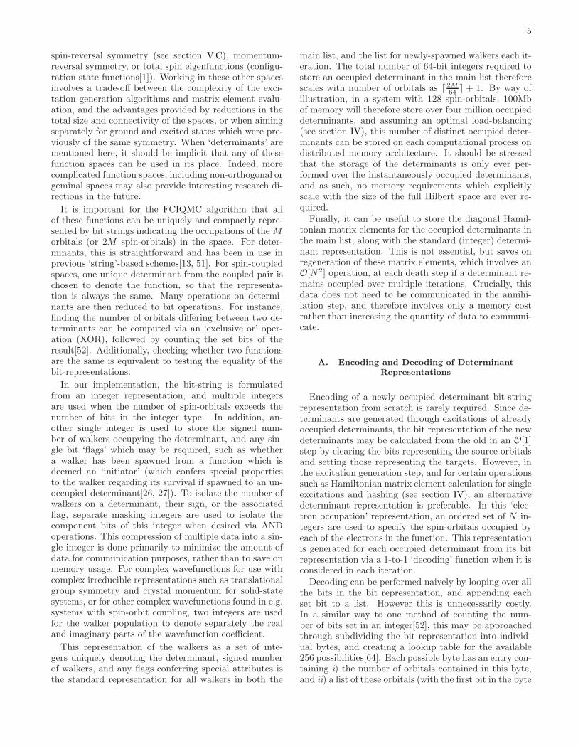
During the iteration, each determinant in the mainwalker array is considered (see section IVB), and at-tempts spawning and death steps. Each time a newwalker is spawned, its hash value is computed betweenthe range of available computational processes, giving itstarget process, and the bit-representation stored in a non-contiguous ‘spawned’ array, separate to the main walkerarray, on the process on which it was created. This ad-ditional spawned array of walkers only needs to store themaximum number of successful spawning events on eachprocess per iteration (Ns), and so can be much smallerthan the main array, by a factor of 10-1000 (Ns ≪ Nw).The position in the array is determined by the hash,and therefore non-contiguously orders the newly spawnedwalkers by the process on which the determinant shouldbe located after communication, as shown on the left fig-ure in Fig. 2. Local death/cloning events are howeverupdated directly in the main array.

At the end of the main iteration loop, the newlyspawned walkers are sent to their designated processesvia a single, synchronized, collective operation (withinthe MPI library, an MPI AlltoAllv operation). As illus-trated in Fig. 2, due to the way that the newly spawnedwalkers were ordered, this takes the form of a non-contiguous matrix transpose. After this, each process’list of newly spawned walkers only includes walkers as-signed to that process. As a consequence, all walkers onany given determinant will now reside on the same pro-cess. This allows annihilation to occur fully without anyfurther communication. After the movement of walkers,the small, now contiguous newly spawned walker list oneach process is ordered and compressed so that there are

7

1 2 3 4 1 2 3 4

Processors Processors

FIG. 2: Schematic to represent the movement of walkers forthe inter-process communication required for the annihilationstep. The non-contiguously filled array containing the newlyspawned walkers is shown for each process on the left beforethe communication, while the right is the set of walkers on thecorrect process after a single, collective communication stepper iteration. The load imbalance in the number of spawnedwalkers per process is of minor concern compared to the bal-ancing of the number of determinants in the main lists due tothe fact that Ns ≪ Nw, and that the annihilation routine isonly of cost O[Ns].

no multiply specified determinants in the list[65]. Thiscombines newly spawned walkers of the same sign intoone entry in the list, and locally annihilates walkers ofdifferent sign between those spawned in the current iter-ation. The mechanism of further annihilation with en-tries from the main list on the process will be describedin section IVB.

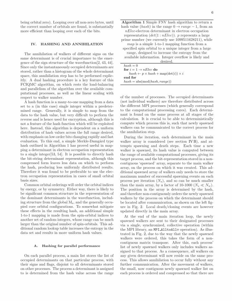
The load-balancing of the algorithm across processes istherefore tied to the uniformity of the hashing function.A beneficial property of the algorithm is the fact that thelarger the system (N), the more entropy that is availableto the hashing function, and therefore the more uniformthe hashing should become. In practice, the load balanc-ing of the hash values is rather uniform and is not thebottleneck of the parallelism. However, this is not theonly consideration, as this algorithm balances the num-ber of occupied determinants across the available pro-cesses rather than the number of walkers, and the equalbalancing of computational effort will depend on both ofthese quantities, as can be seen in Fig. 3.

It is not clear which it would be better to balance,since some operations such as the death step, diagonalmatrix element evaluation and annihilation take placeon the level of occupied determinants, while others suchas the spawning attempts and the majority of the excita-tion generation take place on an individual walker level.The optimal load balancing would include some of bothcharacters, but this algorithm is limited to only considerbalancing of occupied determinants only across compu-tational processes. Therefore, if a walker distribution isheavily skewed towards, say, the Hartree–Fock determi-nant, then this will result in a load-imbalance on the levelof walker distribution across computational processes.

Despite this limitation, an upside of this is that for a

0 500 1000 1500 2000No. processors

0.0

0.1

0.2

0.3

0.4

0.5

0.6

0.7

Ratio load imbalance / average load

Walkers

Determinants

50m walkers100m walkers200m walkers500m walkers

FIG. 3: The observed difference in the number of walkersand occupied determinants between the most and least occu-pied processes relative to the average number per process. Itis notable that the distribution of determinants is substan-tially better balanced than the distribution of walkers. Inthis case, the absolute difference in walker count between themost and least occupied process is roughly equal to the num-ber of walkers on the reference (Hartree–Fock) determinant,and this comes to dominate as the number of processes is in-creased, reducing the average occupancy of each process - aneffect which dominates the parallel scaling.

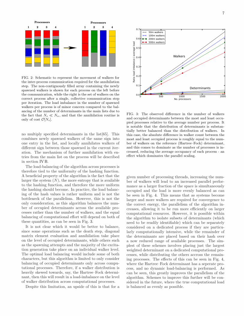
given number of processing threads, increasing the num-ber of walkers will lead to an increased parallel perfor-mance as a larger fraction of the space is simultaneouslyoccupied and the load is more evenly balanced as canbe seen in Fig. 4. This means that as systems becomelarger and more walkers are required for convergence tothe correct energy, the parallelism of the algorithm in-creases, allowing it to be run more efficiently on largercomputational resources. However, it is possible withinthe algorithm to isolate subsets of determinants (whichneed to be readily identifiable) which can be separatelyconsidered on a dedicated process if they are particu-larly computationally intensive, while the remainder ofthe determinants are placed based on their hash overa now reduced range of available processes. The sim-plest of these schemes involves placing just the largestweighted determinant on a dedicated computational pro-cesses, while distributing the others accross the remain-ing processes. The effects of this can be seen in Fig. 4,where the Hartree–Fock determinant has a seperate pro-cess, and no dynamic load-balancing is performed. Ascan be seen, this greatly improves the parallelism of thealgorithm. Schemes to improve this further will be con-sidered in the future, where the true computational loadis balanced as evenly as possible.

8

0 500 1000 1500 2000No. processors

0

10

20

30

40

50

60

70Sp

eedu

p relativ

e to 32 proc

essors

100m walkers500m walkers100m walkers, HF det separate500m walkers, HF det separate

FIG. 4: The observed speed-up as the number of computa-tional processes is increased from 32 to 2048. We note thatthe scaling improves as the number of walkers in the systemis increased. Empirically we observe that the computationalspeed scales fairly efficiently so long as at least 1 million walk-ers are present on each computational process. In systemswhere the walker distribution is skewed to a single occupieddeterminant, such as the Hartree–Fock determinant, it is ad-vantageous to the parallelism of the algorithm to assign a ded-icated process to the storage of this determinant, as shown.

B. Hashing for main walker list

The second hashing is not for the purposes of paral-lelism and involves the explicit construction of a hashtable for the storage of the main walker list on each pro-cess. The idea is for the hash value of a determinantto return a position in a hash table, which will in turnprovide the array index for the determinant in the mainwalker list on the local process. The reason for the hashtable construction is that the time taken to search for adeterminant in the main list, insert a new determinantor delete an old determinant is O[1]. Two integer arraysin memory are required in addition to the main walkerlist. The first is the hash table, which can be of variablelength, but should optimally scale with the size of themain determinant array to minimize hash collisions. Theother is a circular array indexing the vacant positions inthe main determinant list into which new determinantscan be placed. This latter list has a maximum size givenby the length of the main determinant list, but can beshorter [66].

In the main loop, the occupied determinant list is se-quentially accessed. Each time an empty entry in thelist is found, the position index is saved in the circularlist. Spawning and death steps are performed as nor-mal for entries corresponding to occupied determinantsin the list. If all walkers on a determinant are killed dur-

ing the death step, then its walker count is set to zero,and its index is added to the circular list and removedfrom the hash table. Once all walkers on the processhave been considered, there is no need to continue iter-ating through the main walker array, and all further (va-cant) entries in the main determinant list can be consid-ered available for possible walker insertion. In this way,the first entries filled from determinant insertion are theearliest vacant entries, meaning that the main determi-nant list remains as contiguous as possible, minimizingthe number of empty array entries which are searchedthrough.During annihilation, when the contiguous newly

spawned walker list is compared to the existing deter-minants in the main walker list, the hash value of eachdeterminant is computed, and the index of the deter-minant in the array looked up from the hash table. Ifthere are hash collisions (two determinants with the samehash), then multiple entries in the main list may need tobe considered before the correct determinant is found. Ifthe determinant is found, then annihilation or additionto the existing entries can be achieved simply by mod-ification of the number of walkers in the correspondingentry in the main list. If the resultant number of walkersis zero, the entry should be removed from the hash ta-ble, and the associated index added to the circular list offree slots available for determinant insertion, in the sameway as for the death of all walkers on a determinant. Al-ternatively, if no corresponding determinant is found, thenewly spawned walker can be transferred to the main listin the next free position indicated in the circular list. Inthis way, the entire annihilation step can be efficientlyperformed in only O[Ns] computational cost.The reason for the intermediary hash table step to pro-

vide an index is due to the added simplicity when dealingwith hash collisions. This is not essential and could beremoved to provide memory savings. Assuming unifor-mity of the hash values, the probability of a hash collisionbetween two determinants on the same process is givenby

pcollision = 1−Nh!

(Nh −Nd)!NNd

h

, (5)

whereNh is the size of the hash table, andNd denotes thenumber of occupied determinants on the process. It canbe seen in this way that increasing the size of the hashtable is advantageous for minimizing the risk of hash col-lisions. In the case of a hash collision, the additionaldistinct determinant index is included in the same en-try in the hash table, resulting in multiple entries poten-tially being searched at the annihilation stage. Furtherhash collisions are possible, but become scarcer. It is alsoworth mentioning that different random mapping arraysare used in the hashing functions for the distribution overprocesses and over the main determinant array (as wellas different ranges), in order to avoid any unwanted cor-relations being introduced between the two hashes.It is during this annihilation stage that the initiator

9

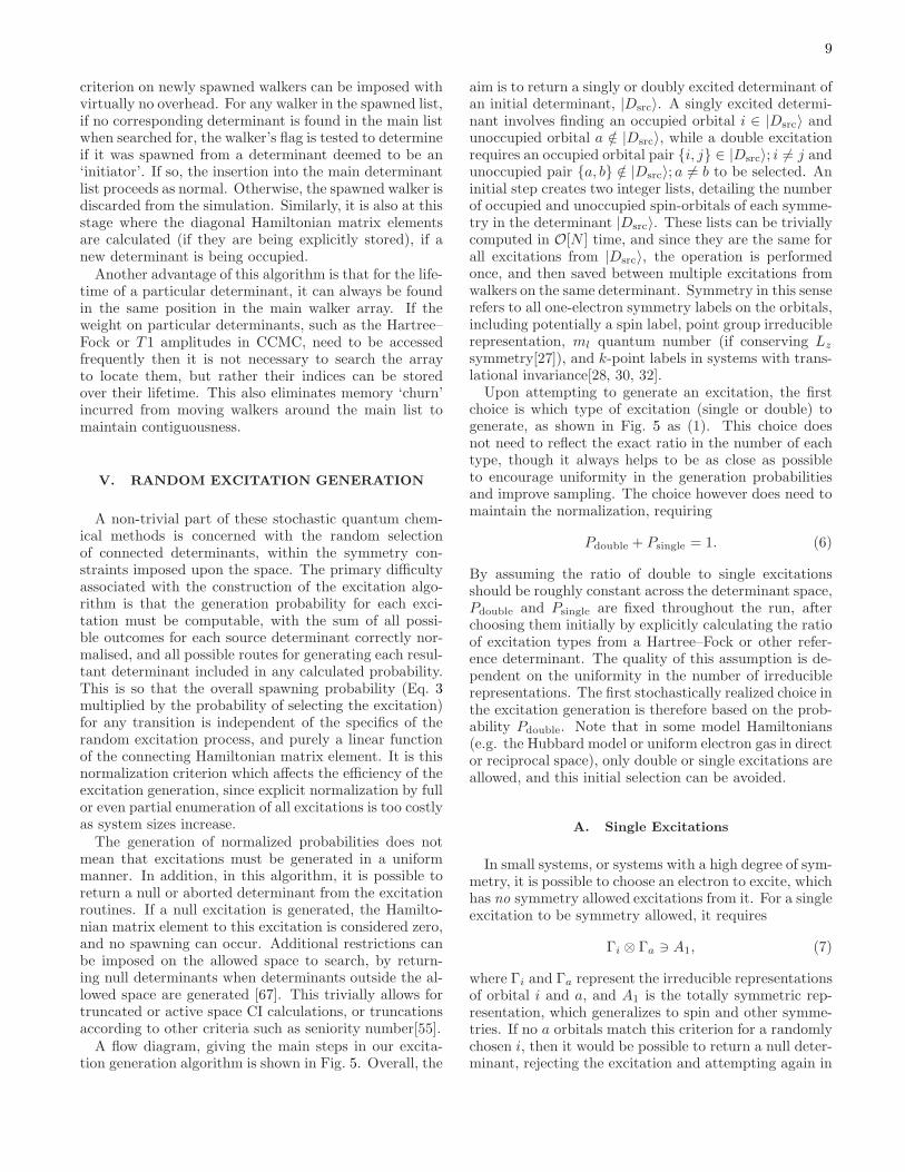
criterion on newly spawned walkers can be imposed withvirtually no overhead. For any walker in the spawned list,if no corresponding determinant is found in the main listwhen searched for, the walker’s flag is tested to determineif it was spawned from a determinant deemed to be an‘initiator’. If so, the insertion into the main determinantlist proceeds as normal. Otherwise, the spawned walker isdiscarded from the simulation. Similarly, it is also at thisstage where the diagonal Hamiltonian matrix elementsare calculated (if they are being explicitly stored), if anew determinant is being occupied.Another advantage of this algorithm is that for the life-

time of a particular determinant, it can always be foundin the same position in the main walker array. If theweight on particular determinants, such as the Hartree–Fock or T 1 amplitudes in CCMC, need to be accessedfrequently then it is not necessary to search the arrayto locate them, but rather their indices can be storedover their lifetime. This also eliminates memory ‘churn’incurred from moving walkers around the main list tomaintain contiguousness.

V. RANDOM EXCITATION GENERATION

A non-trivial part of these stochastic quantum chem-ical methods is concerned with the random selectionof connected determinants, within the symmetry con-straints imposed upon the space. The primary difficultyassociated with the construction of the excitation algo-rithm is that the generation probability for each exci-tation must be computable, with the sum of all possi-ble outcomes for each source determinant correctly nor-malised, and all possible routes for generating each resul-tant determinant included in any calculated probability.This is so that the overall spawning probability (Eq. 3multiplied by the probability of selecting the excitation)for any transition is independent of the specifics of therandom excitation process, and purely a linear functionof the connecting Hamiltonian matrix element. It is thisnormalization criterion which affects the efficiency of theexcitation generation, since explicit normalization by fullor even partial enumeration of all excitations is too costlyas system sizes increase.The generation of normalized probabilities does not

mean that excitations must be generated in a uniformmanner. In addition, in this algorithm, it is possible toreturn a null or aborted determinant from the excitationroutines. If a null excitation is generated, the Hamilto-nian matrix element to this excitation is considered zero,and no spawning can occur. Additional restrictions canbe imposed on the allowed space to search, by return-ing null determinants when determinants outside the al-lowed space are generated [67]. This trivially allows fortruncated or active space CI calculations, or truncationsaccording to other criteria such as seniority number[55].A flow diagram, giving the main steps in our excita-

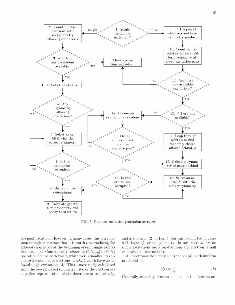
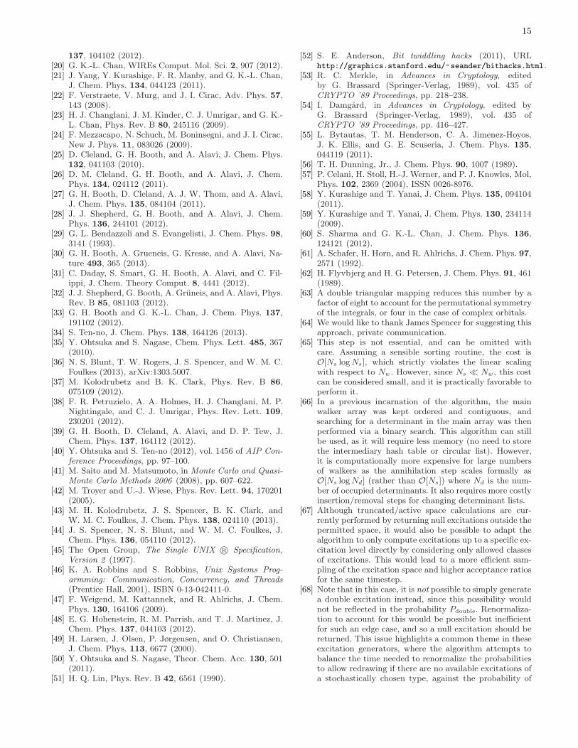
tion generation algorithm is shown in Fig. 5. Overall, the

aim is to return a singly or doubly excited determinant ofan initial determinant, |Dsrc〉. A singly excited determi-nant involves finding an occupied orbital i ∈ |Dsrc〉 andunoccupied orbital a /∈ |Dsrc〉, while a double excitationrequires an occupied orbital pair {i, j} ∈ |Dsrc〉; i 6= j andunoccupied pair {a, b} /∈ |Dsrc〉; a 6= b to be selected. Aninitial step creates two integer lists, detailing the numberof occupied and unoccupied spin-orbitals of each symme-try in the determinant |Dsrc〉. These lists can be triviallycomputed in O[N ] time, and since they are the same forall excitations from |Dsrc〉, the operation is performedonce, and then saved between multiple excitations fromwalkers on the same determinant. Symmetry in this senserefers to all one-electron symmetry labels on the orbitals,including potentially a spin label, point group irreduciblerepresentation, ml quantum number (if conserving Lz

symmetry[27]), and k-point labels in systems with trans-lational invariance[28, 30, 32].Upon attempting to generate an excitation, the first

choice is which type of excitation (single or double) togenerate, as shown in Fig. 5 as (1). This choice doesnot need to reflect the exact ratio in the number of eachtype, though it always helps to be as close as possibleto encourage uniformity in the generation probabilitiesand improve sampling. The choice however does need tomaintain the normalization, requiring

Pdouble + Psingle = 1. (6)

By assuming the ratio of double to single excitationsshould be roughly constant across the determinant space,Pdouble and Psingle are fixed throughout the run, afterchoosing them initially by explicitly calculating the ratioof excitation types from a Hartree–Fock or other refer-ence determinant. The quality of this assumption is de-pendent on the uniformity in the number of irreduciblerepresentations. The first stochastically realized choice inthe excitation generation is therefore based on the prob-ability Pdouble. Note that in some model Hamiltonians(e.g. the Hubbard model or uniform electron gas in director reciprocal space), only double or single excitations areallowed, and this initial selection can be avoided.

A. Single Excitations

In small systems, or systems with a high degree of sym-metry, it is possible to choose an electron to excite, whichhas no symmetry allowed excitations from it. For a singleexcitation to be symmetry allowed, it requires

Γi ⊗ Γa ∋ A1, (7)

where Γi and Γa represent the irreducible representationsof orbital i and a, and A1 is the totally symmetric rep-resentation, which generalizes to spin and other symme-tries. If no a orbitals match this criterion for a randomlychosen i, then it would be possible to return a null deter-minant, rejecting the excitation and attempting again in

10

1. Singleor doubleexcitation?

2. Count numberelectrons withno (symmetry

allowed) excitations

single

3. Are thereany excitations

available?

4. Select an electron

yes

5. Any(symmetryallowed)

excitations?

6. Select an or-bital with the

correct symmetry

yes

7. Is thisorbital un-occupied?

8. Generate newdeterminant

yes

9. Calculate genera-tion probability andparity then return

no

no

10. Pick a pair ofelectrons and takesymmetry product

double

11. Count no. oforbitals which couldform symmetry al-

lowed excitation pairs

12. Are thereany availableexcitations?

13. ≤ 3 orbitalsavailable?

yes

14. Loop throughorbitals to findrandomly chosenallowed orbital, a

yes

15. Choose anorbital, a, at random

no

16. Orbitala unoccupied

and hasavailable pair?

17. Calculate symme-try of paired orbital

yes

18. Select an or-bital, b, with thecorrect symmetry

19. Is thisorbital un-occupied?yes

no

no

Abort excita-tion and returnno

no

FIG. 5: Random excitation generation overview

the next iteration. However, in many cases, this is a com-mon enough occurrence that it is worth renormalizing theallowed choices of i at the beginning of each single excita-tion attempt. Consequently, either an O[Nsym] or O[N ]operation can be performed, whichever is smaller, to cal-culate the number of electrons in |Dsrc〉 which have no al-lowed single excitations, δs. This is most easily calculatedfrom the precalculated symmetry lists, or the electron oc-cupation representation of the determinant respectively,

and is shown in (2) of Fig. 5, but can be omitted in caseswith large M

N, or no symmetry. In rare cases where no

single excitations are available from any electron, a nullexcitation is returned (3).An electron is then chosen at random (4), with uniform

probability of

p(i) =1

N. (8)

Generally, choosing electrons is done on the electron oc-

11

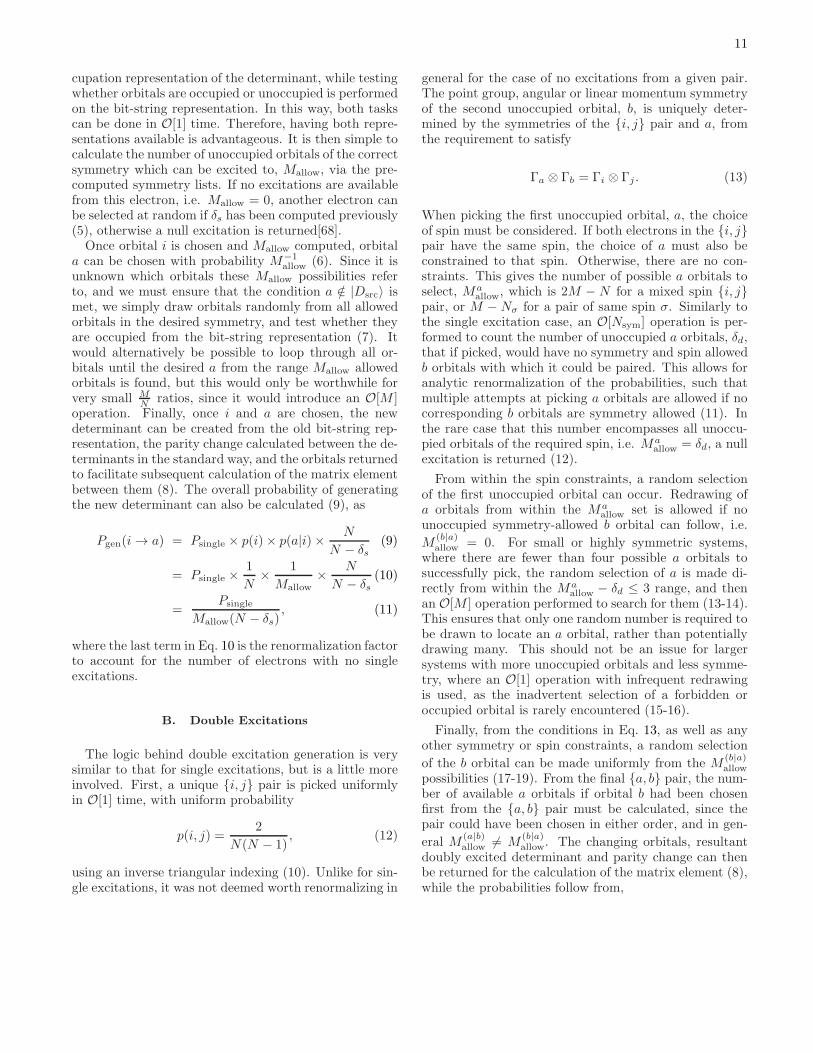
cupation representation of the determinant, while testingwhether orbitals are occupied or unoccupied is performedon the bit-string representation. In this way, both taskscan be done in O[1] time. Therefore, having both repre-sentations available is advantageous. It is then simple tocalculate the number of unoccupied orbitals of the correctsymmetry which can be excited to, Mallow, via the pre-computed symmetry lists. If no excitations are availablefrom this electron, i.e. Mallow = 0, another electron canbe selected at random if δs has been computed previously(5), otherwise a null excitation is returned[68].Once orbital i is chosen and Mallow computed, orbital

a can be chosen with probability M−1allow (6). Since it is

unknown which orbitals these Mallow possibilities referto, and we must ensure that the condition a /∈ |Dsrc〉 ismet, we simply draw orbitals randomly from all allowedorbitals in the desired symmetry, and test whether theyare occupied from the bit-string representation (7). Itwould alternatively be possible to loop through all or-bitals until the desired a from the range Mallow allowedorbitals is found, but this would only be worthwhile forvery small M

Nratios, since it would introduce an O[M ]

operation. Finally, once i and a are chosen, the newdeterminant can be created from the old bit-string rep-resentation, the parity change calculated between the de-terminants in the standard way, and the orbitals returnedto facilitate subsequent calculation of the matrix elementbetween them (8). The overall probability of generatingthe new determinant can also be calculated (9), as

Pgen(i → a) = Psingle × p(i)× p(a|i)×N

N − δs(9)

= Psingle ×1

N×

1

Mallow×

N

N − δs(10)

=Psingle

Mallow(N − δs), (11)

where the last term in Eq. 10 is the renormalization factorto account for the number of electrons with no singleexcitations.

B. Double Excitations

The logic behind double excitation generation is verysimilar to that for single excitations, but is a little moreinvolved. First, a unique {i, j} pair is picked uniformlyin O[1] time, with uniform probability

p(i, j) =2

N(N − 1), (12)

using an inverse triangular indexing (10). Unlike for sin-gle excitations, it was not deemed worth renormalizing in

general for the case of no excitations from a given pair.The point group, angular or linear momentum symmetryof the second unoccupied orbital, b, is uniquely deter-mined by the symmetries of the {i, j} pair and a, fromthe requirement to satisfy

Γa ⊗ Γb = Γi ⊗ Γj . (13)

When picking the first unoccupied orbital, a, the choiceof spin must be considered. If both electrons in the {i, j}pair have the same spin, the choice of a must also beconstrained to that spin. Otherwise, there are no con-straints. This gives the number of possible a orbitals toselect, Ma

allow, which is 2M − N for a mixed spin {i, j}pair, or M − Nσ for a pair of same spin σ. Similarly tothe single excitation case, an O[Nsym] operation is per-formed to count the number of unoccupied a orbitals, δd,that if picked, would have no symmetry and spin allowedb orbitals with which it could be paired. This allows foranalytic renormalization of the probabilities, such thatmultiple attempts at picking a orbitals are allowed if nocorresponding b orbitals are symmetry allowed (11). Inthe rare case that this number encompasses all unoccu-pied orbitals of the required spin, i.e. Ma

allow = δd, a nullexcitation is returned (12).

From within the spin constraints, a random selectionof the first unoccupied orbital can occur. Redrawing ofa orbitals from within the Ma

allow set is allowed if nounoccupied symmetry-allowed b orbital can follow, i.e.

M(b|a)allow = 0. For small or highly symmetric systems,

where there are fewer than four possible a orbitals tosuccessfully pick, the random selection of a is made di-rectly from within the Ma

allow − δd ≤ 3 range, and thenan O[M ] operation performed to search for them (13-14).This ensures that only one random number is required tobe drawn to locate an a orbital, rather than potentiallydrawing many. This should not be an issue for largersystems with more unoccupied orbitals and less symme-try, where an O[1] operation with infrequent redrawingis used, as the inadvertent selection of a forbidden oroccupied orbital is rarely encountered (15-16).

Finally, from the conditions in Eq. 13, as well as anyother symmetry or spin constraints, a random selection

of the b orbital can be made uniformly from the M(b|a)allow

possibilities (17-19). From the final {a, b} pair, the num-ber of available a orbitals if orbital b had been chosenfirst from the {a, b} pair must be calculated, since thepair could have been chosen in either order, and in gen-

eral M(a|b)allow 6= M

(b|a)allow. The changing orbitals, resultant

doubly excited determinant and parity change can thenbe returned for the calculation of the matrix element (8),while the probabilities follow from,

12

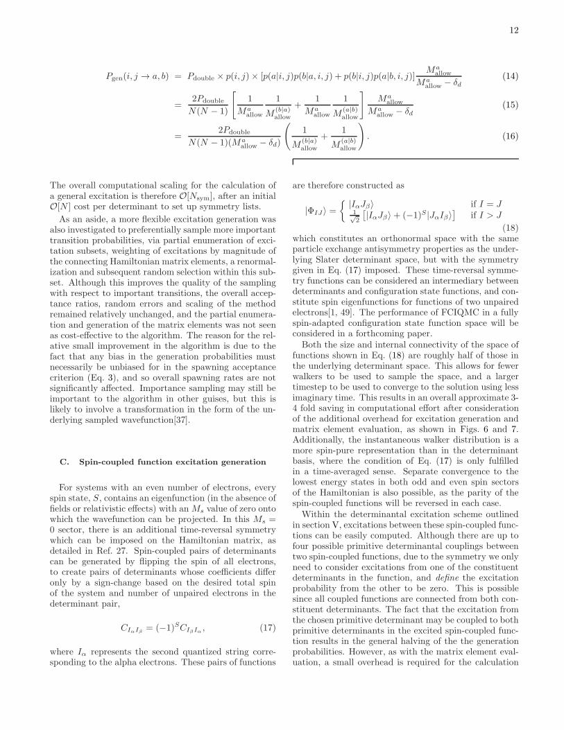
Pgen(i, j → a, b) = Pdouble × p(i, j)× [p(a|i, j)p(b|a, i, j) + p(b|i, j)p(a|b, i, j)]Ma

allow

Maallow − δd

(14)

=2Pdouble

N(N − 1)

[

1

Maallow

1

M(b|a)allow

+1

Maallow

1

M(a|b)allow

]

Maallow

Maallow − δd

(15)

=2Pdouble

N(N − 1)(Maallow − δd)

(

1

M(b|a)allow

+1

M(a|b)allow

)

. (16)

The overall computational scaling for the calculation ofa general excitation is therefore O[Nsym], after an initialO[N ] cost per determinant to set up symmetry lists.

As an aside, a more flexible excitation generation wasalso investigated to preferentially sample more importanttransition probabilities, via partial enumeration of exci-tation subsets, weighting of excitations by magnitude ofthe connecting Hamiltonian matrix elements, a renormal-ization and subsequent random selection within this sub-set. Although this improves the quality of the samplingwith respect to important transitions, the overall accep-tance ratios, random errors and scaling of the methodremained relatively unchanged, and the partial enumera-tion and generation of the matrix elements was not seenas cost-effective to the algorithm. The reason for the rel-ative small improvement in the algorithm is due to thefact that any bias in the generation probabilities mustnecessarily be unbiased for in the spawning acceptancecriterion (Eq. 3), and so overall spawning rates are notsignificantly affected. Importance sampling may still beimportant to the algorithm in other guises, but this islikely to involve a transformation in the form of the un-derlying sampled wavefunction[37].

C. Spin-coupled function excitation generation

For systems with an even number of electrons, everyspin state, S, contains an eigenfunction (in the absence offields or relativistic effects) with an Ms value of zero ontowhich the wavefunction can be projected. In this Ms =0 sector, there is an additional time-reversal symmetrywhich can be imposed on the Hamiltonian matrix, asdetailed in Ref. 27. Spin-coupled pairs of determinantscan be generated by flipping the spin of all electrons,to create pairs of determinants whose coefficients differonly by a sign-change based on the desired total spinof the system and number of unpaired electrons in thedeterminant pair,

CIαIβ = (−1)SCIβIα , (17)

where Iα represents the second quantized string corre-sponding to the alpha electrons. These pairs of functions

are therefore constructed as

|ΦIJ〉 =

{

|IαJβ〉 if I = J1√2

[

|IαJβ〉+ (−1)S |JαIβ〉]

if I > J

(18)which constitutes an orthonormal space with the sameparticle exchange antisymmetry properties as the under-lying Slater determinant space, but with the symmetrygiven in Eq. (17) imposed. These time-reversal symme-try functions can be considered an intermediary betweendeterminants and configuration state functions, and con-stitute spin eigenfunctions for functions of two unpairedelectrons[1, 49]. The performance of FCIQMC in a fullyspin-adapted configuration state function space will beconsidered in a forthcoming paper.Both the size and internal connectivity of the space of

functions shown in Eq. (18) are roughly half of those inthe underlying determinant space. This allows for fewerwalkers to be used to sample the space, and a largertimestep to be used to converge to the solution using lessimaginary time. This results in an overall approximate 3-4 fold saving in computational effort after considerationof the additional overhead for excitation generation andmatrix element evaluation, as shown in Figs. 6 and 7.Additionally, the instantaneous walker distribution is amore spin-pure representation than in the determinantbasis, where the condition of Eq. (17) is only fulfilledin a time-averaged sense. Separate convergence to thelowest energy states in both odd and even spin sectorsof the Hamiltonian is also possible, as the parity of thespin-coupled functions will be reversed in each case.Within the determinantal excitation scheme outlined

in section V, excitations between these spin-coupled func-tions can be easily computed. Although there are up tofour possible primitive determinantal couplings betweentwo spin-coupled functions, due to the symmetry we onlyneed to consider excitations from one of the constituentdeterminants in the function, and define the excitationprobability from the other to be zero. This is possiblesince all coupled functions are connected from both con-stituent determinants. The fact that the excitation fromthe chosen primitive determinant may be coupled to bothprimitive determinants in the excited spin-coupled func-tion results in the general halving of the the generationprobabilities. However, as with the matrix element eval-uation, a small overhead is required for the calculation

13

0.0E+00

5.0E+05

1.0E+06

1.5E+06

2.0E+06

2.5E+06

Num

ber o

f wal

kers

Determinant spaceSpin-coupled space

0 5000 10000 15000 20000 25000 30000 35000 40000Iterations

0.0

0.2

0.4

0.6

0.8

Tim

e pe

r ite

ratio

n / s

Determinant spaceSpin-coupled space

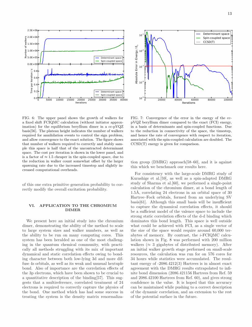
FIG. 6: The upper panel shows the growth of walkers fora fixed shift FCIQMC calculation (without initiator approx-imation) for the equilibrium beryllium dimer in a cc-pVQZbasis[56]. The plateau height indicates the number of walkersrequired for annihilation events to control the sign problem,and allow convergence to the exact solution. The figure showsthat number of walkers required to correctly and stably sam-ple this space is half that of the uncontracted determinantspace. The cost per iteration is shown in the lower panel, andis a factor of ≈ 1.5 cheaper in the spin-coupled space, due tothe reduction in walker count somewhat offset by the largerspawning rate due to the increased timestep and slightly in-creased computational overheads.

of this one extra primitive generation probability to cor-rectly modify the overall excitation probability.

VI. APPLICATION TO THE CHROMIUM

DIMER

We present here an initial study into the chromiumdimer, demonstrating the ability of the method to scaleto large system sizes and walker numbers, as well asthe ability to be run on many computing cores. Thissystem has been heralded as one of the most challeng-ing in the quantum chemical community, with practi-cally all methods struggling with its mix of importantdynamical and static correlation effects owing to bond-ing character between both low-lying 3d and more dif-fuse 4s orbitals, as well as its weak and unusual hextuplebond. Also of importance are the correlation effects ofthe 3p electrons, which have been shown to be crucial toa quantitative description of the binding[57]. This sug-gests that a multireference, correlated treatment of 24electrons is required to correctly capture the physics ofthe bond. One method which has had some success intreating the system is the density matrix renormaliza-

0 20000 40000 60000 80000 100000Iterations

10-5

10-4

10-3

10-2

10-1

Abso

lute

Err

or in

Ene

rgy

/ Eh

Determinant spaceSpin-coupled spaceCCSD(T)

FIG. 7: Convergence of the error in the energy of the cc-pVQZ beryllium dimer compared to the exact (FCI) energy,in a basis of determinants and spin-coupled functions. Dueto the reduction in connectivity of the space, the timestep,and hence the rate of convergence with respect to iteration,associated with the spin-coupled calculation are doubled. TheCCSD(T) energy is given for comparison.

tion group (DMRG) approach[58–60], and it is againstthis which we benchmark our results here.

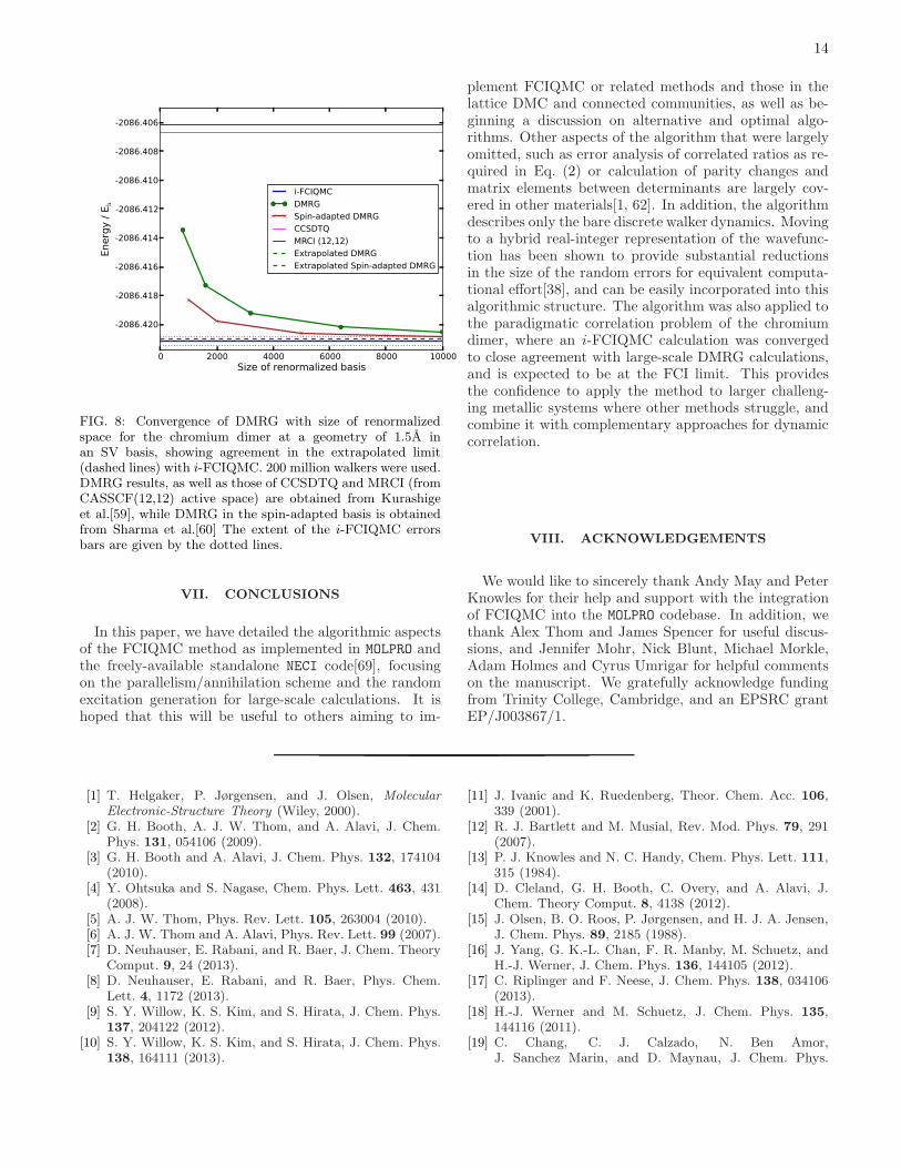
For consistency with the large-scale DMRG study ofKurashige et al.[59], as well as a spin-adapted DMRGstudy of Sharma et al.[60], we performed a single-pointcalculation of the chromium dimer, at a bond length of1.5A, correlating 24 electrons in an orbital space of 30Hartree–Fock orbitals, formed from an underlying SVbasis[61]. Although this small basis will be insufficientto capture the dynamical correlation effects, it shouldbe a sufficient model of the valence space to include thestrong static correlation effects of the d-d binding whichdominates this bond length. This space is well outsidewhat could be achieved with FCI, as a single vector ofthe size of the space would require around 60,000 ter-abytes of memory. By contrast, the i-FCIQMC calcu-lation shown in Fig. 8 was performed with 200 millionwalkers (≈ 3 gigabytes of distributed memory). Afteran initial walker growth stage performed on small-scaleresources, the calculation was run for on 576 cores for34 hours while statistics were accumulated. The resul-tant energy of -2086.4212(3) Hartrees is in almost exactagreement with the DMRG results extrapolated to infi-nite bond dimension (2086.421156 Hartrees from Ref. 59and 2086.42100 Hartrees from Ref. 60), and gives strongconfidence in the value. It is hoped that this accuracycan be maintained while pushing to a correct descriptionof the dynamic correlation, and an extension to the restof the potential surface in the future.

14

0 2000 4000 6000 8000 10000Size of renormalized basis

-2086.420

-2086.418

-2086.416

-2086.414

-2086.412

-2086.410

-2086.408

-2086.406

Energy / E h

i-FCIQMCDMRGSpin-adapted DMRGCCSDTQMRCI (12,12)Extrapolated DMRGExtrapolated Spin-adapted DMRG

FIG. 8: Convergence of DMRG with size of renormalizedspace for the chromium dimer at a geometry of 1.5A inan SV basis, showing agreement in the extrapolated limit(dashed lines) with i-FCIQMC. 200 million walkers were used.DMRG results, as well as those of CCSDTQ and MRCI (fromCASSCF(12,12) active space) are obtained from Kurashigeet al.[59], while DMRG in the spin-adapted basis is obtainedfrom Sharma et al.[60] The extent of the i-FCIQMC errorsbars are given by the dotted lines.

VII. CONCLUSIONS

In this paper, we have detailed the algorithmic aspectsof the FCIQMC method as implemented in MOLPRO andthe freely-available standalone NECI code[69], focusingon the parallelism/annihilation scheme and the randomexcitation generation for large-scale calculations. It ishoped that this will be useful to others aiming to im-

plement FCIQMC or related methods and those in thelattice DMC and connected communities, as well as be-ginning a discussion on alternative and optimal algo-rithms. Other aspects of the algorithm that were largelyomitted, such as error analysis of correlated ratios as re-quired in Eq. (2) or calculation of parity changes andmatrix elements between determinants are largely cov-ered in other materials[1, 62]. In addition, the algorithmdescribes only the bare discrete walker dynamics. Movingto a hybrid real-integer representation of the wavefunc-tion has been shown to provide substantial reductionsin the size of the random errors for equivalent computa-tional effort[38], and can be easily incorporated into thisalgorithmic structure. The algorithm was also applied tothe paradigmatic correlation problem of the chromiumdimer, where an i-FCIQMC calculation was convergedto close agreement with large-scale DMRG calculations,and is expected to be at the FCI limit. This providesthe confidence to apply the method to larger challeng-ing metallic systems where other methods struggle, andcombine it with complementary approaches for dynamiccorrelation.

VIII. ACKNOWLEDGEMENTS

We would like to sincerely thank Andy May and PeterKnowles for their help and support with the integrationof FCIQMC into the MOLPRO codebase. In addition, wethank Alex Thom and James Spencer for useful discus-sions, and Jennifer Mohr, Nick Blunt, Michael Morkle,Adam Holmes and Cyrus Umrigar for helpful commentson the manuscript. We gratefully acknowledge fundingfrom Trinity College, Cambridge, and an EPSRC grantEP/J003867/1.

[1] T. Helgaker, P. Jørgensen, and J. Olsen, Molecular

Electronic-Structure Theory (Wiley, 2000).[2] G. H. Booth, A. J. W. Thom, and A. Alavi, J. Chem.

Phys. 131, 054106 (2009).[3] G. H. Booth and A. Alavi, J. Chem. Phys. 132, 174104

(2010).[4] Y. Ohtsuka and S. Nagase, Chem. Phys. Lett. 463, 431

(2008).[5] A. J. W. Thom, Phys. Rev. Lett. 105, 263004 (2010).[6] A. J. W. Thom and A. Alavi, Phys. Rev. Lett. 99 (2007).[7] D. Neuhauser, E. Rabani, and R. Baer, J. Chem. Theory

Comput. 9, 24 (2013).[8] D. Neuhauser, E. Rabani, and R. Baer, Phys. Chem.

Lett. 4, 1172 (2013).[9] S. Y. Willow, K. S. Kim, and S. Hirata, J. Chem. Phys.

137, 204122 (2012).[10] S. Y. Willow, K. S. Kim, and S. Hirata, J. Chem. Phys.

138, 164111 (2013).

[11] J. Ivanic and K. Ruedenberg, Theor. Chem. Acc. 106,339 (2001).

[12] R. J. Bartlett and M. Musial, Rev. Mod. Phys. 79, 291(2007).

[13] P. J. Knowles and N. C. Handy, Chem. Phys. Lett. 111,315 (1984).

[14] D. Cleland, G. H. Booth, C. Overy, and A. Alavi, J.Chem. Theory Comput. 8, 4138 (2012).

[15] J. Olsen, B. O. Roos, P. Jørgensen, and H. J. A. Jensen,J. Chem. Phys. 89, 2185 (1988).

[16] J. Yang, G. K.-L. Chan, F. R. Manby, M. Schuetz, andH.-J. Werner, J. Chem. Phys. 136, 144105 (2012).

[17] C. Riplinger and F. Neese, J. Chem. Phys. 138, 034106(2013).

[18] H.-J. Werner and M. Schuetz, J. Chem. Phys. 135,144116 (2011).

[19] C. Chang, C. J. Calzado, N. Ben Amor,J. Sanchez Marin, and D. Maynau, J. Chem. Phys.

15

137, 104102 (2012).[20] G. K.-L. Chan, WIREs Comput. Mol. Sci. 2, 907 (2012).[21] J. Yang, Y. Kurashige, F. R. Manby, and G. K.-L. Chan,

J. Chem. Phys. 134, 044123 (2011).[22] F. Verstraete, V. Murg, and J. I. Cirac, Adv. Phys. 57,

143 (2008).[23] H. J. Changlani, J. M. Kinder, C. J. Umrigar, and G. K.-

L. Chan, Phys. Rev. B 80, 245116 (2009).[24] F. Mezzacapo, N. Schuch, M. Boninsegni, and J. I. Cirac,

New J. Phys. 11, 083026 (2009).[25] D. Cleland, G. H. Booth, and A. Alavi, J. Chem. Phys.

132, 041103 (2010).[26] D. M. Cleland, G. H. Booth, and A. Alavi, J. Chem.

Phys. 134, 024112 (2011).[27] G. H. Booth, D. Cleland, A. J. W. Thom, and A. Alavi,

J. Chem. Phys. 135, 084104 (2011).[28] J. J. Shepherd, G. H. Booth, and A. Alavi, J. Chem.

Phys. 136, 244101 (2012).[29] G. L. Bendazzoli and S. Evangelisti, J. Chem. Phys. 98,

3141 (1993).[30] G. H. Booth, A. Grueneis, G. Kresse, and A. Alavi, Na-

ture 493, 365 (2013).[31] C. Daday, S. Smart, G. H. Booth, A. Alavi, and C. Fil-

ippi, J. Chem. Theory Comput. 8, 4441 (2012).[32] J. J. Shepherd, G. Booth, A. Gruneis, and A. Alavi, Phys.

Rev. B 85, 081103 (2012).[33] G. H. Booth and G. K.-L. Chan, J. Chem. Phys. 137,

191102 (2012).[34] S. Ten-no, J. Chem. Phys. 138, 164126 (2013).[35] Y. Ohtsuka and S. Nagase, Chem. Phys. Lett. 485, 367

(2010).[36] N. S. Blunt, T. W. Rogers, J. S. Spencer, and W. M. C.

Foulkes (2013), arXiv:1303.5007.[37] M. Kolodrubetz and B. K. Clark, Phys. Rev. B 86,

075109 (2012).[38] F. R. Petruzielo, A. A. Holmes, H. J. Changlani, M. P.

Nightingale, and C. J. Umrigar, Phys. Rev. Lett. 109,230201 (2012).

[39] G. H. Booth, D. Cleland, A. Alavi, and D. P. Tew, J.Chem. Phys. 137, 164112 (2012).

[40] Y. Ohtsuka and S. Ten-no (2012), vol. 1456 of AIP Con-

ference Proceedings, pp. 97–100.[41] M. Saito and M. Matsumoto, in Monte Carlo and Quasi-

Monte Carlo Methods 2006 (2008), pp. 607–622.[42] M. Troyer and U.-J. Wiese, Phys. Rev. Lett. 94, 170201

(2005).[43] M. H. Kolodrubetz, J. S. Spencer, B. K. Clark, and

W. M. C. Foulkes, J. Chem. Phys. 138, 024110 (2013).[44] J. S. Spencer, N. S. Blunt, and W. M. C. Foulkes, J.

Chem. Phys. 136, 054110 (2012).[45] The Open Group, The Single UNIX R© Specification,

Version 2 (1997).[46] K. A. Robbins and S. Robbins, Unix Systems Prog-

armming: Communication, Concurrency, and Threads

(Prentice Hall, 2001), ISBN 0-13-042411-0.[47] F. Weigend, M. Kattannek, and R. Ahlrichs, J. Chem.

Phys. 130, 164106 (2009).[48] E. G. Hohenstein, R. M. Parrish, and T. J. Martinez, J.

Chem. Phys. 137, 044103 (2012).[49] H. Larsen, J. Olsen, P. Jørgensen, and O. Christiansen,

J. Chem. Phys. 113, 6677 (2000).[50] Y. Ohtsuka and S. Nagase, Theor. Chem. Acc. 130, 501

(2011).[51] H. Q. Lin, Phys. Rev. B 42, 6561 (1990).

[52] S. E. Anderson, Bit twiddling hacks (2011), URLhttp://graphics.stanford.edu/~seander/bithacks.html.

[53] R. C. Merkle, in Advances in Cryptology, editedby G. Brassard (Springer-Verlag, 1989), vol. 435 ofCRYPTO ’89 Proceedings, pp. 218–238.

[54] I. Damgard, in Advances in Cryptology, edited byG. Brassard (Springer-Verlag, 1989), vol. 435 ofCRYPTO ’89 Proceedings, pp. 416–427.

[55] L. Bytautas, T. M. Henderson, C. A. Jimenez-Hoyos,J. K. Ellis, and G. E. Scuseria, J. Chem. Phys. 135,044119 (2011).

[56] T. H. Dunning, Jr., J. Chem. Phys. 90, 1007 (1989).[57] P. Celani, H. Stoll, H.-J. Werner, and P. J. Knowles, Mol,

Phys. 102, 2369 (2004), ISSN 0026-8976.[58] Y. Kurashige and T. Yanai, J. Chem. Phys. 135, 094104

(2011).[59] Y. Kurashige and T. Yanai, J. Chem. Phys. 130, 234114

(2009).[60] S. Sharma and G. K.-L. Chan, J. Chem. Phys. 136,

124121 (2012).[61] A. Schafer, H. Horn, and R. Ahlrichs, J. Chem. Phys. 97,

2571 (1992).[62] H. Flyvbjerg and H. G. Petersen, J. Chem. Phys. 91, 461

(1989).[63] A double triangular mapping reduces this number by a

factor of eight to account for the permutational symmetryof the integrals, or four in the case of complex orbitals.

[64] We would like to thank James Spencer for suggesting thisapproach, private communication.

[65] This step is not essential, and can be omitted withcare. Assuming a sensible sorting routine, the cost isO[Ns logNs], which strictly violates the linear scalingwith respect to Nw. However, since Ns ≪ Nw, this costcan be considered small, and it is practically favorable toperform it.

[66] In a previous incarnation of the algorithm, the mainwalker array was kept ordered and contiguous, andsearching for a determinant in the main array was thenperformed via a binary search. This algorithm can stillbe used, as it will require less memory (no need to storethe intermediary hash table or circular list). However,it is computationally more expensive for large numbersof walkers as the annihilation step scales formally asO[Ns logNd] (rather than O[Ns]) where Nd is the num-ber of occupied determinants. It also requires more costlyinsertion/removal steps for changing determinant lists.

[67] Although truncated/active space calculations are cur-rently performed by returning null excitations outside thepermitted space, it would also be possible to adapt thealgorithm to only compute excitations up to a specific ex-citation level directly by considering only allowed classesof excitations. This would lead to a more efficient sam-pling of the excitation space and higher acceptance ratiosfor the same timestep.

[68] Note that in this case, it is not possible to simply generatea double excitation instead, since this possibility wouldnot be reflected in the probability Pdouble. Renormaliza-tion to account for this would be possible but inefficientfor such an edge case, and so a null excitation should bereturned. This issue highlights a common theme in theseexcitation generators, where the algorithm attempts tobalance the time needed to renormalize the probabilitiesto allow redrawing if there are no available excitations ofa stochastically chosen type, against the probability of

16

this redrawing needing to occur in the first place. From aquality of sampling per iteration perspective, it would beoptimal if we could always return an allowed excitation,but the structure of the algorithm means that it is notalways worthwhile to do so.

[69] Standalone code can be cloned fromhttps://github.com/ghb24/NECI STABLE.git. Pleasefeel free to contact us for assistance with the compilationand running of the program.