arX

iv:q

uant

-ph/

0011

097v

2 1

3 Se

p 20

01

Stochastic description for open quantum systems

Esteban CalzettaDepartamento de Fısica,

Universidad de Buenos Aires, Ciudad Universitaria,

1428 Buenos Aires, Argentina

Albert Roura and Enric Verdaguer ∗

Departament de Fısica Fonamental,

Universitat de Barcelona, Av. Diagonal 647,

08028 Barcelona, Spain

A linear open quantum system consisting of a harmonic oscillator linearly coupled to an infiniteset of independent harmonic oscillators is considered; these oscillators have a general spectral densityfunction and are initially in a Gaussian state. Using the influence functional formalism a formalLangevin equation can be introduced to describe the system’s fully quantum properties even beyondthe semiclassical regime. It is shown that the reduced Wigner function for the system is exactlythe formal distribution function resulting from averaging both over the initial conditions and thestochastic source of the formal Langevin equation. The master equation for the reduced densitymatrix is then obtained in the same way a Fokker-Planck equation can always be derived from aLangevin equation characterizing a stochastic process. We also show that a subclass of quantumcorrelation functions for the system can be deduced within the stochastic description provided bythe Langevin equation. It is emphasized that when the system is not Markovian more informationcan be extracted from the Langevin equation than from the master equation.

I. INTRODUCTION

Feynman observed long ago that the dynamics of an open quantum system may be described in terms of an equivalentstochastic problem [1]. In this paper, we elaborate on this insight by showing that a certain class of quantum Greenfunctions may be obtained directly as ensemble averages in the stochastic formulation. Unlike earlier treatments ofthe origin of stochasticity in the semiclassical limit of quantum theories [2] we do not assume decoherence; rather, weare concerned with the full quantum dynamics of the system.

The stochastic treatment follows from the observation that the Wigner function of the open quantum system maybe represented as the formal distribution function resulting from averaging the solutions of an appropriate Langevinequation both over the initial conditions and the stochastic source. This representation, which is exact for linearsystems, may be extended to nonlinear cases through perturbative methods [3].

We compare the main approaches to the analysis of the stochastic dynamics, namely the Langevin and Fokker-Planck equations, to the corresponding quantum approaches, namely the master equation and the Wigner function.We show that the Fokker-Planck equation is the transport equation for the full Wigner function, and as such it isequivalent to the master equation. The Langevin equation, on the other hand, provides a more detailed description ofthe dynamics, in the sense that the class of correlation functions which may be retrieved from the Langevin equationis larger than the corresponding class for the master or Fokker-Planck equations unless the dynamics is Markovian.

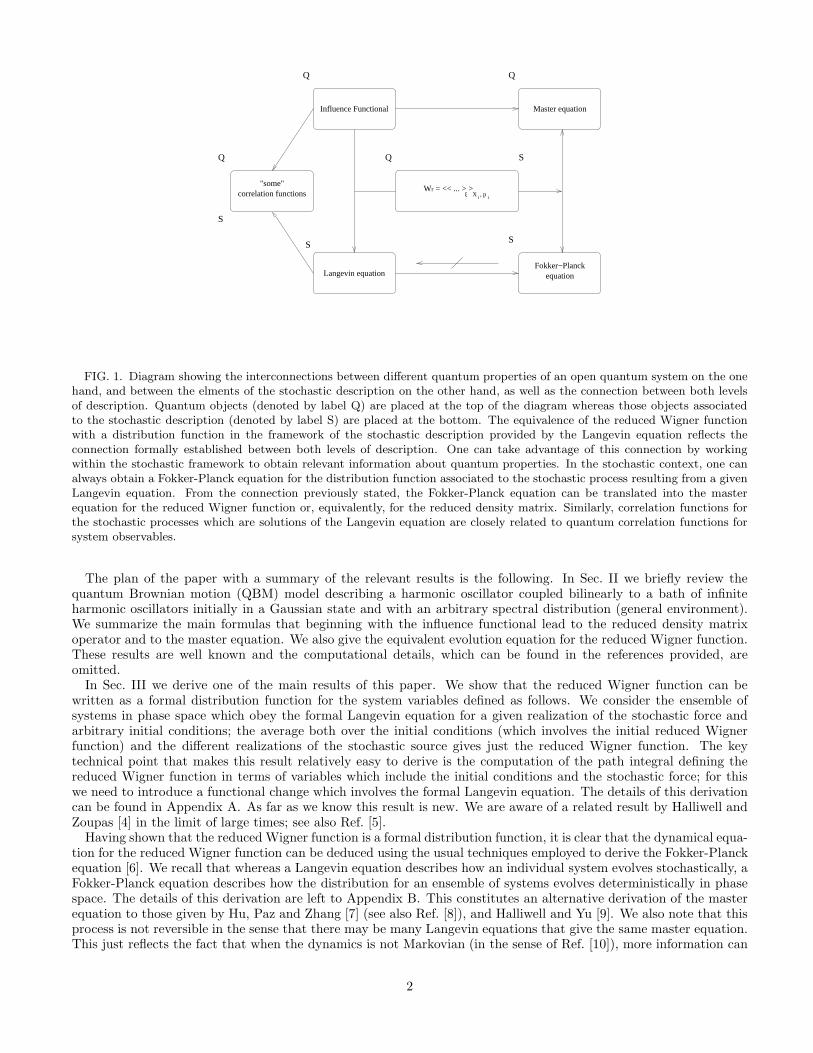
The relationship between these different approaches is summarized in the diagram of Fig. 1. The most fundamentaldescription of the open quantum system is that provided by the Feynman-Vernon influence functional [1]. From this,we may derive the master equation, which gives the dynamics of the reduced density matrix. The integral transformlinking the reduced density matrix to the reduced Wigner function allows us to convert the master equation for theformer into a transport or Fokker-Planck equation for the latter. Feynman’s insight that the influence functional maybe thought as well as an ensemble average over an equivalent stochastic noise allows us to retrieve some correlationfunctions of the quantum problem directly in terms of stochastic averages, while the Fokker-Planck equation associatedto the corresponding Langevin equation gives back the master equation. Thus, the Langevin equation is a very usefultool to gain information on the quantum properties of the system even beyond the semiclassical regime, when it nolonger describes the actual trajectories of the system.

∗Also at Institut de Fısica d’Altes Energies (IFAE), Barcelona, Spain.

1

"some"

Fokker−Planckequation

correlation functions

Influence Functional Master equation

Langevin equation

W = << ... > >rξ X , pi i

Q

QQ

S

S

S

S

Q

FIG. 1. Diagram showing the interconnections between different quantum properties of an open quantum system on the onehand, and between the elments of the stochastic description on the other hand, as well as the connection between both levelsof description. Quantum objects (denoted by label Q) are placed at the top of the diagram whereas those objects associatedto the stochastic description (denoted by label S) are placed at the bottom. The equivalence of the reduced Wigner functionwith a distribution function in the framework of the stochastic description provided by the Langevin equation reflects theconnection formally established between both levels of description. One can take advantage of this connection by workingwithin the stochastic framework to obtain relevant information about quantum properties. In the stochastic context, one canalways obtain a Fokker-Planck equation for the distribution function associated to the stochastic process resulting from a givenLangevin equation. From the connection previously stated, the Fokker-Planck equation can be translated into the masterequation for the reduced Wigner function or, equivalently, for the reduced density matrix. Similarly, correlation functions forthe stochastic processes which are solutions of the Langevin equation are closely related to quantum correlation functions forsystem observables.

The plan of the paper with a summary of the relevant results is the following. In Sec. II we briefly review thequantum Brownian motion (QBM) model describing a harmonic oscillator coupled bilinearly to a bath of infiniteharmonic oscillators initially in a Gaussian state and with an arbitrary spectral distribution (general environment).We summarize the main formulas that beginning with the influence functional lead to the reduced density matrixoperator and to the master equation. We also give the equivalent evolution equation for the reduced Wigner function.These results are well known and the computational details, which can be found in the references provided, areomitted.

In Sec. III we derive one of the main results of this paper. We show that the reduced Wigner function can bewritten as a formal distribution function for the system variables defined as follows. We consider the ensemble ofsystems in phase space which obey the formal Langevin equation for a given realization of the stochastic force andarbitrary initial conditions; the average both over the initial conditions (which involves the initial reduced Wignerfunction) and the different realizations of the stochastic source gives just the reduced Wigner function. The keytechnical point that makes this result relatively easy to derive is the computation of the path integral defining thereduced Wigner function in terms of variables which include the initial conditions and the stochastic force; for thiswe need to introduce a functional change which involves the formal Langevin equation. The details of this derivationcan be found in Appendix A. As far as we know this result is new. We are aware of a related result by Halliwell andZoupas [4] in the limit of large times; see also Ref. [5].

Having shown that the reduced Wigner function is a formal distribution function, it is clear that the dynamical equa-tion for the reduced Wigner function can be deduced using the usual techniques employed to derive the Fokker-Planckequation [6]. We recall that whereas a Langevin equation describes how an individual system evolves stochastically, aFokker-Planck equation describes how the distribution for an ensemble of systems evolves deterministically in phasespace. The details of this derivation are left to Appendix B. This constitutes an alternative derivation of the masterequation to those given by Hu, Paz and Zhang [7] (see also Ref. [8]), and Halliwell and Yu [9]. We also note that thisprocess is not reversible in the sense that there may be many Langevin equations that give the same master equation.This just reflects the fact that when the dynamics is not Markovian (in the sense of Ref. [10]), more information can

2

be extracted from the Langevin equation than from the master equation.In Sec. IV we obtain the second main result of this paper. We show that quantum correlation functions for the system

variables can be obtained within the stochastic description provided by the Langevin equation by explicitly computingthe closed time path (CTP) generating functional for the system. It turns out that this generating functional can bewritten as an average over the initial conditions times a term that depends on the noise kernel, which contains theinformation on the fluctuations induced by the environment on the system.

We also show that quantum correlation functions cannot be obtained using the propagators for the reduced densitymatrix unless the system is Markovian, a fact which is discussed in Appendix C. Note that this is in contrast with aclosed system where the unitary propagators, which are solutions of the Schrodinger equation, allow one to obtain allthe information about the existing quantum correlations.

Finally, in Sec. V we summarize and briefly discuss our results.Throughout the paper we use units in which h = 1 except for Sec. II.

II. INFLUENCE FUNCTIONAL FORMALISM FOR OPEN QUANTUM SYSTEMS

A. A survey of open quantum systems

Open quantum systems [11] are of interest in condensed matter physics [12], quantum optics [13], quantum measure-ment theory [14], nonequilibrium field theory [15–18], quantum cosmology [19] and semiclassical gravity [20]. Amongthe most widely used examples of open quantum system is the QBM model, which consists of a single massive particlein a potential (usually quadratic) interacting with an infinite set of independent harmonic oscillators which are initiallyin a Gaussian state (most often a thermal equilibrium state) [21]. The coupling may be linear both in the systemand environment variables or may be nonlinear in some or all of these variables. The frequencies of the environmentoscillators are distributed according to a prescribed spectral density function, the simplest case corresponding to theso-called ohmic environment. The linear coupling provides a good description of many open quantum systems incondensed matter physics [22,12], but in field theory [23], quantum cosmology [19] and semiclassical gravity [24,25]the coupling is usually nonlinear. Part of the interest of the linear systems is that they are in many cases exactlysolvable and detailed studies of different aspects of open quantum systems can be performed. One of the issues thathas received much attention in recent years is environment-induced decoherence as a mechanism to understand thetransition from the quantum to the classical regime [26,27].

Concepts such as the Feynman-Vernon influence functional method, the reduced density matrix, the reduced Wignerfunction, the master equation, the Fokker-Planck equation and the Langevin equation are some of the key wordsassociated to the study of open quantum systems. One of the purposes of this paper is to review the place of theseconcepts in the QBM model and to establish their often subtle interrelations. Thus, let us first review some of thoseconcepts and recall their main features.

The reduced density matrix is defined from the density matrix of the whole closed system by tracing out theenvironment. Its dynamical evolution may be given in terms of the Feynman and Vernon influence functional [1]. Theinfluence functional is defined from a path integral involving the action of the system and the environment and anintegration of the environment degrees of freedom. Its use in the QBM model is widespread especially since Caldeiraand Leggett were able to compute in closed form the propagator for the reduced density matrix in the case of linearcoupling with an ohmic environment [22].

The master equation is a differential equation describing the evolution of the reduced density matrix. The masterequation for linear coupling and ohmic environment at high temperature was first deduced by Caldeira and Leggett[22], it was extended to arbitrary temperature by Unruh and Zurek [28], and it was finally obtained for a generalenvironment (i.e. for an arbitrary spectral density function) by Hu, Paz and Zhang [7]. This result can be extendedto the case of nonlinear coupling by treating the interaction perturbatively up to quadratic order [29].

Closely related to the reduced density matrix is the reduced Wigner function (in fact one goes from one to the otherby an integral transform) [30,31]. The reduced Wigner function is similar in many aspects to a distribution functionin phase-space, although it is not necessarily positive definite, and the dynamical equation it satisfies is similar tothe Fokker-Planck equation for classical statistical systems [32,33]. This equation is, of course, entirely equivalentto the master equation for the reduced density matrix and, sometimes, we also refer to it as the master equation.The reduced density matrix has been used to study decoherence induced by the environment [34–37,28,7,29]. TheWigner function has also been used in studies of emergence of classicality induced by an environment [38], especiallyin quantum cosmology [19].

The Langevin equation [39,6] is another relevant equation for open quantum systems. This equation has either beenintroduced phenomenologically [33] to describe the effect of the environment into a classical system (Brownian motion)

3

or it has been derived within the functional approach (see, however, Refs. [40] and [41] for a quantum version of theLangevin equation in operator language) as a classical or semiclassical limit. Thus, Gell-Mann and Hartle [2,42] inthe framework of the consistent histories approach to quantum mechanics [43] considered the decoherence functional,which is closely related to the influence functional in the case of open quantum systems, to measure the degree ofclassicality of the system. They were able to show that under certain conditions there exists a semiclassical limit inan open system which may be suitably described by a Langevin equation with the self-correlation of the stochasticsource given by the noise kernel which appears in the decoherence functional.

Langevin-type equations as a suitable tool to study the semiclassical limit have been used recently in semiclassicalgravity and cosmology [24,44,25]. In inflationary cosmology they have been used to describe the stochastic effect onthe inflaton field [45–51] or the stochastic behavior of large-scale gravitational perturbations [52], which is importantfor cosmological structure formation.

B. A linear QBM model

Here we review a QBM model as an example of a linear open quantum system. Let us consider a harmonic oscillatorof mass M , the “system”, coupled to a bath of independent harmonic oscillators of mass m, the “environment”. Forsimplicity, let us assume that the system and environment are linearly coupled. The action for the whole set of degreesof freedom is defined by:

S[x, qj] = S[x] + S[qj] + Sint[x, qj], (2.1)

where the terms on the right-hand side, which correspond to the action of the system, the environment and theinteraction term respectively, are given by

S[x] =

∫

dt(1

2Mx2 −

1

2MΩ2x2), (2.2)

S[qj] =∑

j

∫

dt(1

2mq2

j −1

2mω2

j q2j ), (2.3)

Sint[x, qj] =∑

j

cj

∫

dtx(t)qj(t) =

∫

∞

0

dω2mω

πc(ω)I(ω)

∫

dtx(t)q(t; ω), (2.4)

where we introduced the spectral density I(ω) =∑

j πc2j (2mωj)

−1δ(ω − ωj) in the last equality, c(ω) and q(t; ω) are

functions such that c(ωj) = cj and q(t; ωj) = qj(t), with cj being system-environment coupling parameters, and Ωand ωj are, respectively, the system and environment oscillator frequencies.

The reduced density matrix for an open quantum system is defined from the density matrix ρ of the whole systemby tracing out the environment degrees of freedom:

ρr(xf , x′

f , tf ) =

∫

∏

j

dqjρ(xf , qj, x′

f , qj, tf ). (2.5)

The evolution for the reduced density matrix, which is in general nonunitary and even non-Markovian, can be writtenas

ρr(xf , x′

f , tf) =

∫

dxidx′

iJ(xf , x′

f , tf ; xi, x′

i, ti)ρr(xi, x′

i, ti), (2.6)

where the propagator J is defined in a path integral representation by

J(xf , x′

f , tf ; xi, x′

i, ti) =

x(tf )=xf∫

x(ti)=xi

Dx

x′(tf )=x′

f∫

x′(ti)=x′

i

Dx′ei(S[x]−S[x′]+SIF [x,x′])/h, (2.7)

where SIF [x, x′] is the influence action introduced by Feynman and Vernon [1]. When the system and the environmentare initially uncorrelated, i.e., when the initial density matrix factorizes (ρ(ti) = ρr(ti)⊗ ρe(ti), where ρr(ti) and ρe(ti)

4

mean, respectively, the density matrix operators of the system and the environment at the initial time) and the initial

density matrix for the environment ρe(q(i)j , q

′(i)j , ti) is Gaussian, one obtains [1,22]:

SIF [x, x′] = −2

∫ tf

ti

ds

∫ s

ti

ds′∆(s)D(s, s′)X(s′) +i

2

∫ tf

ti

ds

∫ tf

ti

ds′∆(s)N(s, s′)∆(s′), (2.8)

where X(s) ≡ (x(s) + x′(s))/2 and ∆(s) ≡ x′(s) − x(s). The kernels D(s, s′) and N(s, s′) are called the dissipationand noise kernel, respectively. When the bath is initially in thermal equilibrium these kernels are related by the usualfluctuation-dissipation relation [53]. When no special form is assumed for the spectral density I(ω), this is usuallyreferred to as a general environment. One of the most common particular cases is the so-called Ohmic environment,defined by I(ω) ∼ ω (some high frequency cut-off may be sometimes naturally introduced).

Starting with Eqs. (2.5) and (2.7) a differential equation for the system’s reduced density matrix, known as themaster equation, can be derived. The expression for a general environment was first obtained by Hu, Paz and Zhang[7]; see also Ref. [9] for an alternative derivation:

ih∂ρr

∂t= −

h2

2M

(

∂2

∂x2−

∂2

∂x′2

)

ρr +1

2MΩ2(x2 − x′2)ρr +

1

2MδΩ2(t)(x2 − x′2)ρr

−ihA(t)(x − x′)

(

∂

∂x−

∂

∂x′

)

ρr + hB(t)(x − x′)

(

∂

∂x+

∂

∂x′

)

ρr − iMC(t)(x − x′)2ρr, (2.9)

where the functions δΩ2(t), A(t), B(t) and C(t) represent a frequency shift, a dissipation factor and two diffusivefactors, respectively. For explicit expressions of these functions see Appendix B. An alternative representation forthe system reduced density matrix is the reduced Wigner function Wr(X, p, t) defined as

Wr(X, p, t) =1

2πh

∫

∞

−∞

d∆eip∆/hρr(X − ∆/2, X + ∆/2, t). (2.10)

It follows immediately that the master equation (2.9) can be written in the following equivalent form:

∂Wr

∂t= HR, WrPB + 2A(t)

∂(pWr)

∂p+ hB(t)

∂2Wr

∂X∂p+ hMC(t)

∂2Wr

∂p2, (2.11)

where HR, WrPB ≡ −(p/M)∂Wr/∂X + MΩ2R(t)X∂Wr/∂p with Ω2

R(t) = Ω2 + δΩ2(t). This equation is formallysimilar to the Fokker-Planck equation for a distribution function.

III. STOCHASTIC DESCRIPTION OF THE SYSTEM’S QUANTUM DYNAMICS

In this Section we show that the reduced Wigner function can be written as a formal distribution function for somestochastic process, and using this result we deduce the corresponding Fokker-Planck equation.

A. Reduced density matrix and Wigner function

To find an explicit expression for the reduced density matrix (2.5) at a time tf , we need to compute the pathintegrals which appear in Eq. (2.7) for the reduced density matrix propagator. On the other hand, the reducedWigner function Wr is related to the reduced density matrix by the integral transform (2.10). In Appendix A, weshow that Wr can be written in the following suggestive form:

Wr(Xf , pf , tf ) =

⟨

⟨

δ(X(tf ) − Xf )δ(MX(tf ) − pf )⟩

ξ

⟩

Xi,pi

, (3.1)

where

〈. . .〉ξ ≡ [det(2πN)]−

1

2

∫

Dξ . . . e−1

2ξ·N−1

·ξ, (3.2)

〈. . .〉Xi,pi≡

∫

∞

−∞

dXi

∫

∞

−∞

dpi . . . Wr(Xi, pi, ti). (3.3)

5

and X (t) is the solution with initial conditions Xi, pi of the Langevin-like equation

(L · X)(t) = ξ(t), (3.4)

where L(t, t′) ≡ M(

d2

dt′2 + Ω2ren

)

δ(t− t′) + H(t, t′). Here the functions Ωren and H(t, t′) are defined below Eq. (A1),

and we have also used the notation A · B ≡∫ tf

tidt A(t)B(t).

Thus, the reduced Wigner function can be interpreted as an average over a Gaussian stochastic process ξ(t) with〈ξ(t)〉ξ = 0 and 〈ξ(t)ξ(t′)〉ξ = N(t, t′) as well as an average over the initial conditions characterized by a distribution

function Wr(Xi, pi, ti). It is only after formally interpreting ξ(t) as a stochastic process characterized by Eq. (3.2)that Eq. (3.4) can be regarded as a Langevin equation. Note that, in general, Eq. (3.4) is not meant to describe theactual trajectories of the system.

Note, in addition, that although Wr(Xi, pi, ti) is real, which follows from the hermiticity of the density matrix,and properly normalized, in general it is not positive everywhere (except for Gaussian states) and, thus, cannot beconsidered as a probability distribution. The fact that the Wigner function cannot be interpreted as a phase-spaceprobability density is crucial since most of the nonclassical features of the quantum state are tightly related to theWigner function having negative values. For instance, a coherent superposition state is typically characterized by theWigner function presenting strong oscillations with negative values in the minima [38,37], which are closely connectedto interference terms.

Equation (3.1) is the main result of this Section and shows that the reduced Wigner function can be interpreted as aformal distribution in phase space. This result will now be used to derive the corresponding Fokker-Planck equation.

B. From Langevin to Fokker-Planck: recovery of the master equation

As mentioned above there is a simple one-to-one correspondence between any density matrix and the associatedWigner function introduced in (2.10). Taking this correspondence into account, the equation satisfied by the reducedWigner function is equivalent to the master equation satisfied by the reduced density matrix. By deriving Eq. (3.1)with respect to time and using the Langevin-type equation in (3.4), one can obtain a Fokker-Planck differentialequation describing the time evolution of the system’s reduced Wigner function. The details of the calculation canbe found in Appendix B. Our result is the transport equation (B16) which is written in terms of the time dependentcoefficients A(t), B(t) and C(t) defined, respectively, by Eqs. (B10), (B17) and (B18). These coefficients are, of course,in agreement with those previously derived in Refs. [9] and [7]; see also [8]. Thus, this is yet another alternative wayto derive the master or transport equation (2.11).

This new road to the transport equation highlights the fact that while one can derive the Fokker-Planck equationfrom the Langevin equation, the opposite is not possible in general. One can always consider Langevin equationswith stochastic sources characterized by different noise kernels which, nevertheless, lead to the same Fokker-Planckequation and, thus, the same master equation. This can be argued from the expressions obtained in the derivation ofthe Fokker-Planck equation. Let us consider, for simplicity, the situation corresponding to local dissipation. A localcontribution to the noise gives no contribution to B(t), but it does contribute to C(t) as can be seen from Eqs. (B17)and (B18) taking into account that Gret(t, t) = 0 and ∂Gret(t

′, t)/∂t′|t′=t = M−1. Thus, one can always choose anynoise kernel that gives the desired B(t) and then add the appropriate local contribution to the noise kernel to get thedesired C(t) keeping B(t) fixed. Note that changing the noise kernel does not change A(t). To illustrate the fact thatthere exist different noise kernels giving the same B(t), as was stated above, one may consider the particular casecorresponding to the weak dissipation limit so that Gret(t, t

′) ∼ (MΩ)−1 sin Ω(t − t′)θ(t − t′). To see that a different

N(t, t′) giving the same B(t) as N(t, t′) exists reduces then to show that there is at least one nontrivial function

ν(s, t) = N(t, t′) − N(t, t′) (with s = t − t′) such that for any t we have∫ t

0 ds sin(Ωs)ν(s, t) = 0, which can be shownto be the case.

The fact that different Langevin equations lead to the same master equation1 reflects that the former contains moreinformation than the latter. This fact can be qualitatively understood in the following way. In the influence functional

1In fact, what we showed was that a Langevin equation contains in general more information that the corresponding Fokker-Planck equation. To extend this assertion to the master equation, one should make sure that the different Langevin equationsleading to the same Fokker-Planck equation can be obtained from an influence functional. This fact seems plausible providedthat one considers general Gaussian initial states for the environment.

6

it is only the evolution of the environment degrees of freedom that is traced out. Of course, having integrated over allthe possible quantum histories for the environment, no correlations in the environment can be obtained. Nevertheless,since the system is interacting with the environment, non-Markovian correlations for the system at different timesmay in general persist. On the other hand, when considering either the reduced density matrix or its propagator,also the system evolution, except for the final state, is integrated out. Consequently, information on non-Markoviancorrelations for the system is no longer available. Thus, only when the system’s reduced dynamics is Markovian, i.e.

the influence functional is local in time, we expect that the Langevin equation and the master equation contain thesame information. In particular, for a Gaussian stochastic source, as in our case, the Langevin equation containsthe information about the system correlations at different times which the Fokker-Planck equation cannot in generalaccount for. Only in the case in which the dynamics generated by the Langevin equation is Markovian one cancompute the correlation functions just from the solutions of the Fokker-Planck equation or, equivalently, the masterequation for the propagator J(x2, x

′

2, t2; x1, x′

1, t1); see Eq. (2.7). The key point is the fact that the propagator for thereduced density matrix only factorizes when the influence action is local. In Appendix C we give a detailed argumenton this point.

It is important to note that for a closed quantum system the evolution determined by the time evolution operatorsU(t2, t1) obtained from the Schrodinger equation is always unitary and, thus, also Markovian. That is why theSchrodinger equation suffices to get the correlation functions for a closed quantum system. On the contrary, foran open quantum system the evolution is nonunitary and, provided that the influence action is nonlocal, not evenMarkovian.

IV. CORRELATION FUNCTIONS

We have seen that the reduced Wigner function, or equivalently the reduced density matrix, and the master equationgoverning these functions can be obtained from a formal stochastic description provided by the Langevin equation(3.4). In this Section we show that also entirely quantum correlation functions for the system can be obtained bymeans of the stochastic description developed in the previous Section.

A. CTP generating functional for the system and n-point quantum correlation functions

All the relevant quantum correlation functions for the system can be obtained from the CTP generating functional,which is expressed, after integrating out the environment, as [54,55]:

ZCTP [J, J ′] =

∫

dxf

∫

dxidx′

i

x(tf )=xf∫

x(ti)=xi

Dx

x′(tf )=xf∫

x′(ti)=x′

i

Dx′eiJ·x−iJ′·x′

ei(S[x]−S[x′]+SIF [x,x′])ρr(xi, x′

i, ti), (4.1)

where use was made of the influence action introduced in Eq. (2.7). Equivalently, we may rewrite the previous equationchanging to semisum and difference variables with JΣ = (J(t) + J ′(t))/2 and J∆ = J ′(t) − J(t), integrate the systemaction by parts and proceed analogously as we did in Appendix A to obtain

ZCTP [JΣ, J∆] =⟨

e−iJ∆·Xo⟩

Xi,pie−

1

2J∆·Gret·N ·(J∆·Gret)

T

e−iJ∆·Gret·JΣ . (4.2)

where X0(t) is the solution to the homogeneous equation (L · X)(t) = 0 with the initial conditions Xi, pi. It isinteresting to note that the first factor in Eq. (4.2) contains all the information about the initial conditions of thesystem, whereas the information about the fluctuations induced on the system by the environment is essentiallycontained in the second factor through the noise kernel. This is the key result of this Section, which will allow torelate the quantum with the stochastic correlation functions.

Any n-point quantum correlation function for the system position operators can be obtained from the CTP gener-ating functional according to the equation

Tr[

(T x(t1) . . . x(tm)) ρ(ti)(

T x(tm+1) . . . x(tm+n))]

= in−m

(

δ

δJ

)m(δ

δJ ′

)n

ZCTP [J, J ′]

∣

∣

∣

∣

J,J′=0

. (4.3)

Since one can always write J and J ′ in terms of JΣ and J∆, the right-hand side of Eq. (4.3) can be expressed as alinear combination of terms of the type

7

ir+s

(

δ

δJΣ

)r (δ

δJ∆

)s

ZCTP [JΣ, J∆]

∣

∣

∣

∣

JΣ,J∆=0

, (4.4)

with 0 ≤ r ≤ n + m, 0 ≤ s ≤ n + m and r + s = n + m. To obtain an explicit expression one must evaluate Eq. (4.4)with the final result for the CTP generating functional (4.2).

B. Quantum correlation functions from stochastic averages

Using the expression (4.4) for the case r = 0, a connection can be established between the correlation functionsfor the Gaussian stochastic process associated to ξ(t) via the Langevin-type equation (3.4) with Wr(Xi, pi, ti) as thedistribution function for the initial conditions, and some quantum correlation functions corresponding to quantumexpectation values of products of Heisenberg operators at different instants of time. Any correlation function for theformer stochastic process can be obtained from its characteristic functional in the usual way:

⟨

〈X(t1) . . . X(ts)〉ξ

⟩

Xi,pi

= is(

δ

δK

)s⟨

⟨

e−i K·X⟩

ξ

⟩

Xi,pi

∣

∣

∣

∣

K=0

. (4.5)

The generating functional for the aforementioned stochastic process is, in turn, related to the full CTP generatingfunctional previously introduced as follows:

⟨

⟨

e−i K·X⟩

ξ

⟩

Xi,pi

= ZCTP [JΣ = 0, J∆ = K]. (4.6)

Substituting Eq. (4.6) into Eq. (4.5), rewriting J∆ in terms of J and J ′, and using expression (4.3), we can express thecorrelation functions for the stochastic process in terms of quantum correlation functions for the system observables.In particular, for s = 2 we have

⟨

〈X(t1)X(t2)〉ξ

⟩

Xi,pi

=1

4

[

〈T x(t1)x(t2)〉 + 〈x(t1)x(t2)〉 + 〈x(t2)x(t1)〉 +⟨

T x(t1)x(t2)⟩]

=1

2〈x(t1), x(t2)〉 , (4.7)

where, as usual, we used 〈. . .〉 to denote the quantum expectation value Tr[. . . ρ(ti)].On the other hand, concentrating on the stochastic description provided by the left-hand side of Eq. (4.7) and

elaborating a little bit on it by using Eq. (A6) and taking into account that ξ(t) is a Gaussian stochastic processcharacterized by 〈ξ(t)〉ξ = 0 and 〈ξ(t1)ξ(t2)〉ξ = N(t1, t2), we can write

⟨

〈X(t1)X(t2)〉ξ

⟩

Xi,pi

=⟨

〈[Xo(t1) + (Gret · ξ)(t1)] [Xo(t2) + (Gret · ξ)(t2)]〉ξ

⟩

Xi,pi

= 〈Xo(t1)Xo(t2)〉Xi,pi+ (Gret · N · (Gret)

T )(t1, t2). (4.8)

Hence, the final result is

1

2〈x(t1), x(t2)〉 = 〈Xo(t1)Xo(t2)〉Xi,pi

+ (Gret · N · (Gret)T )(t1, t2). (4.9)

The left-hand side of Eq. (4.9) is the quantum correlation function, which can therefore be described within thestochastic scheme in terms of two separate contributions: the first term on the right-hand side corresponds entirely tothe dispersion in the initial conditions, whereas the second term is due to the fluctuations induced by the stochasticsource appearing in the Langevin-type equation (3.4). It should be remarked that, as discussed in Appendix C, forthe general case of a nonlocal influence action no quantum correlation functions (except for the trivial case of n = 1)can be expressed in terms of the propagators for the reduced density matrix, which can be obtained from the masterequation.

It is clear from Eqs. (4.5) and (4.6) that only those quantum correlation functions which are obtained by functionallydifferentiating the CTP generating functional with respect to J∆ (but not JΣ) an arbitrary number of times can berelated to the stochastic correlation functions (4.5). Let us, therefore, see what is the general expression for allthe quantum correlation functions that can be directly obtained from the stochastic description. We begin with theclassical correlation functions (4.5) for the stochastic processes X(t) which are solutions of the Langevin-type equationwith stochastic source ξ(t) and initial conditions averaged over the initial reduced Wigner function. Then we writethese correlation functions in terms of path integrals and use the results of Secs. III and IV to relate them to a subclassof quantum correlation functions for the system:

8

⟨

〈X(t1) . . . X(tn)〉ξ

⟩

Xi,pi

= [det(2πN)]−1

2

∫

∞

−∞

dXf

∫

∞

−∞

dXi

∫

∞

−∞

dpi

∫

Dξe−1

2ξ·N−1

·ξ

δ(X(tf ) − Xf )X(t1) . . . X(tn)Wr(Xi, piti) = Tr∗[

X(t1) . . . X(tn)ρ(ti)]

, (4.10)

with X(tj) = (x(tj) + x′(tj))/2 and

Tr∗ [x(t1) . . . x′(tr) . . . x(ts) . . . x′(tu) . . . ρ(ti)] ≡ Tr [T x(t1) . . . x(tr−1)x(ts) . . . x(tu−1)

ρ(ti)

T x(tr) . . . x(ts−1)x(tu) . . .]

, (4.11)

where both the initial density matrix and the trace correspond to the whole closed quantum system (i.e., system plus

environment) and T and T denote time and anti-time ordering, respectively. It is then straightforward to show that

⟨

〈X(t1) . . . X(tn)〉ξ

⟩

Xi,pi

= 2−nn∑

m=0

1

m!(n − m)!

∑

σ∈Sn

Tr

T

σ(m)∏

j=σ(1)

x(tj)

ρ(ti)

T

σ(n)∏

k=σ(m+1)

x(tk)

, (4.12)

where σ ∈ Sn are all the possible permutations for a set consisting of n elements.

V. SUMMARY AND DISCUSSION

In this paper we have considered the stochastic description of a linear open quantum system. We have shownthat the reduced Wigner function can be written as a formal distribution function for a stochastic process given by aLangevin-type equation. The master equation has then been deduced as the corresponding Fokker-Planck equation forthe stochastic process. We have also shown that a subclass of quantum correlation functions for the system variablescan be written in terms of stochastic correlation functions. Our results are summarized in the diagram of Fig. 1 whichshow all the interconnections between the influence functional, the Langevin equation, the Fokker-Planck equation,the master equation and the correlation functions.

Finally, we stress that although we have exploited the formal description of open quantum systems in terms ofstochastic processes, a classical statistical interpretation is not always possible. Thus, although the Wigner functionis a real and properly normalized function providing a distribution for the initial conditions of our formal stochasticprocesses, it is not a true probability distribution function in the sense that it is not positive definite in general. Infact, this property is crucial for the existence of quantum coherence for the system. Nevertheless, even though theLangevin equation does not in general describe actual classical trajectories (histories) of the system, it is still a veryuseful tool to compute quantum correlation functions or even as an intermediate step to derive the master equation.Note that, after all, in statistical mechanics one uses Langevin equations basically to compute correlation functions.It is remarkable that in the light of our results the use of Langevin equations in semiclassical gravity or in inflationarycosmology may provide more information about genuine quantum properties of the gravitational field than previouslysuspected, and its use as an intermediate step between the semiclassical limit and a quantum theory seems justified.

ACKNOWLEDGMENTS

We are grateful to Rosario Martın for interesting discussions and to Daniel Arteaga for a careful reading of themanuscript. This work has been partially supported by the CICYT Research Project No. AEN98-0431 and byFundacion Antorchas under grant A-13622/1-21. E. C. acknowledges support from Universidad de Buenos Aires,CONICET, Fundacion Antorchas and ANPCYT through grant 03-05229. A. R. also acknowledges partial supportof a grant from the Generalitat de Catalunya, and E. V. also acknowledges support from the Spanish Ministery ofEducation under the FPU grant PR2000-0181 and the University of Maryland for hospitality.

9

APPENDIX A: DERIVATION OF THE STOCHASTIC REPRESENTATION FOR THE WIGNER

FUNCTION

Let us begin by rewriting the influence action (2.8) as

SIF [x, x′] =

∫ tf

ti

ds

∫ tf

ti

ds′∆(s)Hbare(s, s′)X(s′) +

i

2

∫ tf

ti

ds

∫ tf

ti

ds′∆(s)N(s, s′)∆(s′)

≡ X · Hbare · ∆ +i

2∆ · N · ∆, (A1)

where we used the notation A ·B ≡∫ tf

tidt A(t)B(t), and defined Hbare(s, s

′) as formally equivalent to −2D(s, s′)θ(s−

s′). Being the product of two distributions the latter expression is not well defined in general and suitable regularizationand renormalization may be required; see Ref. [56] for details. The local divergences present in Hbare(s, s

′) = H(s, s′)+Hdiv(s)δ(s− s′) can be canceled by suitable counterterms Ωdiv in the bare frequency of the system Ω = Ωren + Ωdiv.From now on we will consider that this infinite renormalization, if necessary, has already been performed so that bothΩren and H(s, s′) are free of divergences. Now we perform three main steps.

First, we integrate the system action by parts:

S[x] − S[x′] = −M

∫ tf

ti

dt(X(t)∆(t) − Ω2renX(t)∆(t)) = − MX∆

∣

∣

∣

tf

ti

+ M

∫ tf

ti

dt∆(t)

(

d2

dt2+ Ω2

ren

)

X(t). (A2)

Second, we perform the Gaussian path integral for ∆(t). Taking into account that the value of the Jacobian

determinant for the change of integration variables∫ xf

xiDx∫ x′

f

x′

i

Dx′ −→∫ Xf

XiDX

∫∆f

∆iD∆ is one, the Gaussian path

integral for ∆(t) with ∆i and ∆f fixed is performed:

∫ Xf

Xi

DX

∫ ∆f

∆i

D∆ei∆·L·Xe−1

2∆·N ·∆ =

(

detN

2π

)−1

2∫ Xf

Xi

DXe−1

2(L·X)·N−1

·(L·X), (A3)

where L(t, t′) ≡ M(

d2

dt′2 + Ω2ren

)

δ(t − t′) + H(t, t′). The integration over ∆i gives,

ρr(Xf − ∆f/2, Xf + ∆f/2, tf) =

(

detN

2π

)−1

2∫

∞

−∞

d∆i

∫

∞

−∞

dXi

∫ Xf

Xi

DXe−1

2(L·X)·N−1

·(L·X)

e−iMXf ∆f eiMXi∆iρr(Xi − ∆i/2, Xi + ∆i/2, ti)

= 2π

(

detN

2π

)−1

2∫

∞

−∞

dXi

∫ Xf

Xi

DXe−1

2(L·X)·N−1

·(L·X)

e−iMXf ∆f Wr(Xi, MXi, ti), (A4)

where in the last step we used Eq. (2.10), which defines the reduced Wigner function.Third, we carry out the following functional change:

X(t) −→

Xi = X(ti), pi ≡ MXi = MX(ti), ξ(t) = (L · X)(t)

. (A5)

Note that with this change the function X(t) gets substituted by the initial conditions (Xi, pi) and the function ξ(t)in the functional integration. It is important to note that at this point the function ξ(t) is not a stochastic process butjust a function over which a path integral is performed. The functional change (A5) is invertible as can be explicitlyseen:

Xi, pi, ξ(t) −→ X(t) = X0(t) +

∫ t

ti

dt′Gret(t, t′)ξ(t′), (A6)

where Gret(t′, t′′) is the retarded (i.e., Gret(t

′, t′′) = 0 for t′ ≤ t′′) Green function for the linear integro-differential

operator associated to the kernel L(t, t′), and Xi(t) =∫ t

tidt′Gret(t, t

′)ξ(t′) is a solution of the inhomogeneous equation

(L · Xi)(t) = ξ(t) with initial conditions Xi(ti) = 0 and ∂Xi(t′)/∂t′|t′=ti

= 0. On the other hand, X0(t) is a solution

of the homogeneous equation (L ·X0)(t) = 0, with initial conditions X0(ti) = Xi and X(ti) = pi/M . Since the change

10

is linear, the Jacobian functional determinant will be a constant (this can be clearly seen by skeletonizing the pathintegral). After performing the functional change, we obtain

ρr(Xf − ∆f/2, Xf + ∆f/2, tf) = K

∫

∞

−∞

dXi

∫

∞

−∞

dpi

∫

Dξδ(X(tf ) − Xf )e−1

2ξ·N−1

·ξe−iMX(tf )∆f Wr(Xi, pi, ti),

where the delta function δ(X(tf ) − Xf ) was introduced to restrict the functional integral∫

Dξ with free ends, in

order to take into account the restriction on the final points of the allowed paths for the integral∫Xf DX appearing

in Eq. (A4). The contribution from the Jacobian has been included in the constant K. In order to determine thisconstant, we demand the reduced density matrix to remain normalized, i.e., that Trρr(tf ) = 1 if Trρr(ti) = 1:

1 =

∫

∞

−∞

dXfρr(Xf , Xf , tf ) = K

∫

dXf

∫

Dξδ(X(tf ) − Xf )e−1

2ξ·N−1

·ξ

∫

∞

−∞

dXi

∫

∞

−∞

dpiWr(Xi, pi, ti)

= K

∫

Dξe−1

2ξ·N−1

·ξ

∫

∞

−∞

dXi

∫

∞

−∞

dpiWr(Xi, pi, ti).

Now, from Eq. (2.10) it can be checked that Trρr(ti) = 1 implies∫

∞

−∞dXi

∫

∞

−∞dpiWr(Xi, pi, ti) = 1. The constant

K is thus determined to be

K =

[∫

Dξe−1

2ξ·N−1

·ξ

]−1

= [det(2πN)]−

1

2 . (A7)

Finally, using the definition (2.10) for the Wigner function and the fact that

1

2π

∫

∞

−∞

d∆feipf ∆f e−iMX(tf )∆f = δ(MX(tf ) − pf ),

we get an expression for the reduced Wigner function

Wr(Xf , pf , tf ) = K

∫

∞

−∞

dXi

∫

∞

−∞

dpi

∫

Dξδ(X(tf ) − Xf )δ(MX(tf ) − pf )e−1

2ξ·N−1

·ξWr(Xi, pi, ti), (A8)

which can be written as Eq. (3.1).

APPENDIX B: DERIVATION OF THE FOKKER-PLANCK EQUATION

The derivation of a Fokker-Planck equation from a Langevin equation with local dissipation is well understood, seeRef. [6]. However, in our case the existence of nonlocal dissipation makes it convenient to review the main steps. Letus begin by computing ∂Wr/∂t from expression (3.1),

∂Wr(X, p, t)

∂t=

⟨

⟨

X(t)δ′(X(t) − X)δ(MX(t) − p)⟩

ξ

⟩

Xi,pi

+

⟨

⟨

δ(X(t) − X)MX(t)δ′(MX(t) − p)⟩

ξ

⟩

Xi,pi

= −p

M

∂Wr(X, p, t)

∂X−

∂

∂p

⟨

⟨

δ(X(t) − X)MX(t)δ(MX(t) − p)⟩

ξ

⟩

Xi,pi

, (B1)

where the fact that X(t), ∂/∂X(t) and ∂/∂X(t) may be replaced by p/M , −∂/∂X and −∂/∂p respectively, since theyare multiplying the delta functions, was used in the second equality. Let us now concentrate on the expectation valueappearing in the last term and recall the expectation values defined in (3.2)-(3.3). We will consider the Langevin-typeequation

(L · X)(t′) = ξ(t′), (B2)

corresponding to the functional change (A5) and substitute the corresponding expression for MX(t) so that the lastexpectation value in (B1) can be written as

− MΩ2renXWr(X, p, t) +

⟨

⟨(

−

∫ t

ti

dtH(t, t′)X(t′) + ξ(t)

)

δ(X(t) − X)δ(MX(t) − p)

⟩

ξ

⟩

Xi,pi

. (B3)

11

Any solution of Eq. (B2) can be written as

X(t′) = Xh(t′) +

∫ t

ti

dt′′Gadv(t′, t′′)ξ(t′′), (B4)

where Xh(t′) is a solution of the homogeneous equation (L · X)(t′) = 0 such that Xh(t) = X , Xh(t) = p/M and

Gadv(t′, ‘t′′) is the advanced (i.e. , Gadv(t′, t′′) = 0 for t′ ≥ t′′) Green function for the linear integro-differential operator

associated to the kernel L(t, t′). The particular solution of the inhomogeneous Eq. (B2) Xi(t′) =

∫ t

tidt′′Gadv(t

′, t′′)ξ(t′′)

has boundary conditions Xi(t) = 0, ∂Xi(t′)/∂t′

∣

∣

∣

t′=t= 0. Both Xh(t′) and Gadv(t′, t′′) can be expressed in terms of

the homogeneous solutions u1(t′) and u2(t

′), which satisfy u1(ti) = 1, u1(t) = 0 and u2(ti) = 0, u2(t) = 1 respectively:

Xh(t′) = X

(

u2(t′) −

u2(t)

u1(t)u1(t

′)

)

+(p/M)

u1(t)u1(t

′), (B5)

Gadv(t′, t′′) = −

1

M

u1(t′)u2(t

′′) − u2(t′)u1(t

′′)

u1(t′′)u2(t′′) − u2(t′′)u1(t′′)θ(t′′ − t′). (B6)

We use the advanced propagator so that there is no dependence on the initial conditions at time t′ = ti coming fromthe homogeneous solution but just on the final conditions at time t′ = t, i.e., on those the Fokker-Planck equation iswritten in terms of. Using expression (B4) the first term within the expectation value appearing in Eq. (B3) can bereexpressed as

∫ t

ti

dtH(t, t′)

⟨

⟨

X(t′)δ(X(t) − X)δ(MX(t) − p)⟩

ξ

⟩

Xi,pi

=

∫ t

ti

dt′H(t, t′)Xh(t′)Wr(X, p, t) +

∫ t

ti

dt′∫ t

ti

dt′′H(t, t′)Gadv(t′, t′′)

⟨

⟨

ξ(t′′)δ(X(t) − X)δ(MX(t) − p)⟩

ξ

⟩

Xi,pi

. (B7)

The first term on the right-hand side can in turn be written as

− (MδΩ(t)X + 2A(t)p) Wr(X, p, t), (B8)

where

δΩ(t) =1

M

∫ t

ti

dt′H(t, t′)[u2(t′) − (u2(t)/u1(t))u1(t

′)], (B9)

A(t) =1

2(Mu1(t))

−1

∫ t

ti

dt′H(t, t′)u1(t′). (B10)

In order to find an expression for⟨

ξ(t′)δ(X(t) − X)δ(MX(t) − p)⟩

ξwe use Novikov’s formula for Gaussian stochas-

tic processes [57], which corresponds essentially to use (3.2) and functionally integrate by parts with respect to ξ(t),

〈ξ(t′)F (t; ξ]〉ξ =

∫ t

ti

dt′′N(t′, t′′) 〈δF (t; ξ]/δξ(t′′)〉ξ . (B11)

We then obtain the following expression:

⟨

ξ(t′)δ(X(t) − X)δ(MX(t) − p)⟩

ξ= −

∫ t

ti

dt′′N(t′, t′′)

⟨(

δX(t)

δξ(t′′)

∂

∂X+ M

δX(t)

δξ(t′′)

∂

∂p

)

δ(X(t) − X)δ(MX(t) − p)⟩

ξ(B12)

where we used again the presence of the delta functions to substitute the functional derivatives δ/δX(t′′′) and δ/δX(t′′′)by δ(t′′′ − t) · ∂/∂X and δ(t′′′ − t) · M · ∂/∂p, respectively, in the second equality. Functionally differentiating with

respect to ξ(t′′) expression (A6) for X(t) and analogously for X(t) we get

12

δX(t′)

δξ(t′′)= Gret(t

′, t′′), (B13a)

δX(t′)

δξ(t′′)=

∂

∂t′Gret(t

′, t′′), (B13b)

which after substitution into (B12) leads to

⟨

⟨

ξ(t′)δ(X(t) − X)δ(MX(t) − p)⟩

ξ

⟩

Xi,pi

= −

∫ t

ti

dt′′N(t′, t′′)

(

Gret(t, t′′)

∂

∂X+ M

∂Gret(t, t′′)

∂t

∂

∂p

)

Wr(X, p, t).

(B14)

The retarded Green function can also be expressed in terms of the solutions of the homogeneous equation u1(t) andu2(t), which were previously introduced, as

Gret(t′, t′′) =

1

M

u1(t′)u2(t

′′) − u2(t′)u1(t

′′)

u1(t′′)u2(t′′) − u2(t′′)u1(t′′)θ(t′ − t′′). (B15)

Note that it is important to use now the expression in terms of the retarded propagator Gret and the initial conditionsXi and pi (at time t′ = ti), since the “final” conditions X(t) and MX(t) depend on ξ(t′′) (for t′′ < t). Putting all theterms together, i.e., (B3), (B7) and (B14), we reach the final expression for (B1):

∂Wr

∂t= HR, WrPB + 2A(t)

∂(pWr)

∂p+ B(t)

∂2Wr

∂X∂p+ MC(t)

∂2Wr

∂p2, (B16)

where the Poisson bracket is defined following Eq. (2.11) (with ΩR = Ωren+δΩ), δΩ(t) and A(t) are given by Eqs. (B9)and (B10), and

B(t) =

∫ t

ti

dt′′′N(t, t′′′)Gret(t, t′′′) −

∫ t

ti

dt′H(t, t′)

∫ t

ti

dt′′Gadv(t′, t′′)

∫ t

ti

dt′′′N(t′′, t′′′)Gret(t, t′′′), (B17)

C(t) =

∫ t

ti

dt′′′N(t, t′′′)∂Gret(t, t

′′′)

∂t−

∫ t

ti

dt′H(t, t′)

∫ t

ti

dt′′Gadv(t′, t′′)

∫ t

ti

dt′′′N(t′′, t′′′)∂Gret(t, t

′′′)

∂t. (B18)

The last two expressions were obtained by combining the second term within the expectation value appearing in (B3)and the second term on the right-hand side of Eq. (B7). It should be taken into account that if we put back the h’s,there appears one with every noise kernel in Eqs. (B17) and (B18).

APPENDIX C: CORRELATION FUNCTIONS AND NONLOCAL INFLUENCE ACTION

Let us see how the fact that the influence action is nonlocal implies that the propagator for the reduced densitymatrix does not factorize in time and, thus, the system evolution is non-Markovian. In this Appendix we will denotethe integrand of the real part of the influence action by H ≡ ∆(t)H(t, t′)X(t′) and the integrand of the imaginarypart by N ≡ ∆(t)N(t, t′)∆(t′)/2.

When the influence action is local H(t, t′) ≡ H(t)δ(t − t′), N (t, t′) ≡ N(t)δ(t − t′) and we have

SIF [x, x′; tf , ti) =

∫ tf

ti

dt

∫ tf

ti

dt′H + i

∫ tf

ti

dt

∫ tf

ti

dt′N =

∫ tf

ti

dtH + i

∫ tf

ti

dtN, (C1)

where we introduced the notation SIF [x, x′; tf , ti), which is a functional of x(t) and x′(t) and also depends on thevariables ti and tf , to explicitly state the initial and final times defining the dependence domain considered for thefunctions x(t) and x′(t), which will play an important role in the subsequent discussion. Expression (C1) can then bedecomposed as follows

SIF [x, x′; tf , ti) =

(∫ tf

t1

dtH + i

∫ tf

t1

dtN

)

+

(∫ t1

ti

dtH + i

∫ t1

ti

dtN

)

= SIF [x, x′; tf , t1) + SIF [x, x′; t1, ti), (C2)

so that the influence functional factorizes

13

FIF [x, x′; tf , ti) = eiSIF [x,x′;tf ,ti) = FIF [x, x′; tf , t1)FIF [x, x′; t1, ti), (C3)

and so does the reduced density matrix propagator, as can be straightforwardly seen from its path integral represen-tation

J(xf , x′

f , tf ; xi, x′

i, ti) =

x(tf )=xf∫

x(ti)=xi

Dx

x′(tf )=x′

f∫

x′(ti)=x′

i

Dx′ei(S[x]−S[x′]+SIF [x,x′;tf ,ti))

=

∫

dx1dx′

1

x(tf )=xf∫

x(t1)=x1

Dx

x′(tf )=x′

f∫

x′(t1)=x′

1

Dx′ei(S[x]−S[x′]+SIF [x,x′;tf ,t1))

×

x(t1)=x1∫

x(ti)=xi

Dx

x′(t1)=x′

1∫

x′(ti)=x′

i

Dx′ei(S[x]−S[x′]+SIF [x,x′;t1,ti))

=

∫

dx1dx′

1J(xf , x′

f , tf ; x1, x′

1, t1)J(x1, x′

1, t1; xi, x′

i, ti), (C4)

where use was made both of the fact that the system action is local and (C3) applied to definition (2.7) for the reduceddensity matrix propagator. This property allows one to obtain the quantum correlation functions for the system fromthe propagators of the reduced density matrix, which are solutions of the master equation. To illustrate this fact,consider as an example the quantum correlation function 〈x(t2)x(t1)〉 with t2 > t1, defined by:

Tr [x(t2)x(t1)ρ(ti)] =

x(tf )=xf∫

Dx

x′(tf )=x′

f∫

Dx′x(t2)x(t1)ei(S[x]−S[x′]+SIF [x,x′;tf ,ti))ρr(xi, x

′

i, ti)

=

∫

dxidx′

i

∫

dx2dx′

2x2

∫

dx1dx′

1x1J(xf , x′

f , tf ; x2, x′

2, t2)

J(x2, x′

2, t2; x1, x′

1, t1)J(x1, x′

1, t1; xi, x′

i, ti)ρr(xi, x′

i, ti). (C5)

Here the path integrals in the intermediate steps were decomposed in a way completely analogous to that used in(C4). Hence, the information on the correlation functions can be essentially obtained from the master equation whenthe influence action is local.

On the other hand, when the influence action is nonlocal,

SIF [x, x′; tf , ti) =

∫ tf

ti

dt

∫ tf

ti

dt′H + i

∫ tf

ti

dt

∫ tf

ti

dt′N

=

(∫ t1

ti

dt

∫ t1

ti

dt′H +

∫ t1

ti

dt

∫ tf

t1

dt′H +

∫ tf

t1

dt

∫ t1

ti

dt′H +

∫ tf

t1

dt

∫ tf

t1

dt′H

)

+i

(∫ t1

ti

dt

∫ t1

ti

dt′N +

∫ t1

ti

dt

∫ tf

t1

dt′N +

∫ tf

t1

dt

∫ t1

ti

dt′N +

∫ tf

t1

dt

∫ tf

t1

dt′N

)

. (C6)

The cross terms like∫ t1

tidt∫ tf

t1dt′N do not allow the influence action to be separated into terms that depend either on

the “history” of the system just for times smaller than t1 or just for times greater than t1 (as happened in Eq. (C2)).This fact makes it impossible to factorize the influence functional as was done in Eq. (C3) and consequently impliesthat neither the reduced density matrix propagators factorize in the sense of Eq. (C4) nor the quantum correlationfunctions can be obtained from the reduced density matrix propagators as was done in Eq. (C5). It is, thus, clearhow the nonlocality of the influence action leads to a non-Markovian evolution for the system and the impossibilityto obtain the correlation functions from the propagators for the reduced density matrix.

[1] R.P. Feynman and F.L. Vernon, Ann. Phys. (N.Y.) 24, 118 (1963); R.P. Feynman and A.R. Hibbs, Quantum Mechanics

and Path Integrals (McGraw-Hill, New York, 1965).

14

[2] M. Gell-Mann and J.B. Hartle, Phys. Rev. D 47, 3345 (1993).[3] E. Calzetta, A. Roura end E. Verdaguer, Phys. Rev. D in press, hep-ph/0106091.[4] J.J. Halliwell and A. Zoupas, Phys. Rev. D 52, 7294 (1995); ibid. 55, 4697 (1997).[5] J. Anglin and S. Habib, Mod. Phys. Lett. A 11, 2655 (1996).[6] J.M. Sancho and M. San Miguel, Z. Phys. B 36, 357 (1979); 43 361 (1981).[7] B.L. Hu, J.P. Paz, and Y. Zhang, Phys. Rev. D 45, 2843 (1992).[8] J.P. Paz, in The Physical Origin of Time Asymmetry, edited by J.J. Halliwell, J. Perez-Mercader and W.H. Zurek (Cam-

bridge University Press, Cambridge, England, 1994).[9] J.J. Halliwell and T. Yu, Phys. Rev. D 53, 2012 (1996).

[10] J.P. Paz and W.H. Zurek, Phys. Rev. D 48, 2728 (1993).[11] E.B. Davies, Quantum theory of open systems (Academic Press, London, 1976).[12] A.O. Caldeira and A.J. Leggett, Ann. Phys. (N.Y.) 149, 374 (1983); A.J. Leggett et al., Rev. Mod. Phys. 59, 1 (1987).[13] D.F. Walls and G.J. Milburn, Quantum optics (Springer, Berlin, 1994).[14] W.H. Zurek, Phys. Rev. D 24, 1516 (1981); ibid. 26, 1862 (1982).[15] E. Calzetta and B.L. Hu, Phys. Rev. D 37, 2878 (1988).[16] E. Calzetta and B.L. Hu, Phys. Rev. D 61, 025012 (2000).[17] G.J. Stephens, E. Calzetta, B.L. Hu, and S.A. Ramsey, Phys. Rev. D 59, 045009 (1999).[18] E. Calzetta, B.L. Hu, and S.A. Ramsey, Phys. Rev. D 61, 125013 (2000).[19] S. Habib, Phys. Rev. D 42, 2566 (1990); S. Habib and R. Laflamme ibid. 42, 4056 (1990); J.P. Paz and S. Sinha, ibid. 44,

1038 (1991); ibid. 45, 2823 (1992).[20] B.L. Hu, Physica A 158, 399 (1989).[21] R. Zwanzig, Phys. of Fluids 2, 12 (1959); R. Rubin, J. Math. Phys. 1, 309 (1960); ibid. 2, 373 (1961); G. Ford, M. Kac

and P. Mazur, ibid. 6, 504 (1963).[22] A.O. Caldeira and A.J. Leggett, Physica 121A, 587 (1983).[23] E. Calzetta and B.L. Hu, Phys. Rev. D 55, 3536 (1997).[24] E. Calzetta and B.L. Hu, Phys. Rev. D 49, 6636 (1994); B.L. Hu and A. Matacz, ibid. 51, 1577 (1995); B.L. Hu and

S. Sinha, ibid. 51, 1587 (1995); A. Campos and E. Verdaguer, ibid. 53, 1927 (1996); E. Calzetta, A. Campos and E.Verdaguer, ibid. 56, 2163 (1997).

[25] E. Calzetta and E. Verdaguer, Phys. Rev. D 59, 083513 (1999).[26] W.H. Zurek, Physics Today 44, 36 (1991); Prog. Theor. Phys. 81, 281 (1993).[27] J.P. Paz and W.H. Zurek, in Coherent Matter Waves, Les Houches Session LXXII, edited by R. Kaiser, C. Westbrook and

F. David), 533 (Springer, Berlin, 2001).[28] W.G. Unruh and W.H. Zurek, Phys. Rev. D 40, 1071 (1989).[29] B.L. Hu, J.P. Paz, and Y. Zhang, Phys. Rev. D 47, 1576 (1993).[30] E.P. Wigner, Phys. Rev. 40, 749 (1932).[31] M. Hillery, R.F. O’Connell, M.O. Scully and E.P. Wigner, Phys. Rep.106, 121 (1984).[32] N. Wax (editor), Selected papers on noise and stochastic processes (Dover, 1954); C.W. Gardiner, Handbook of Stochastic

Processes (Springer, Berlin, 1983).[33] H. Risken, The Fokker-Planck Equation (Springer-Verlag, Berlin, 1989).[34] E. Joos and H.D. Zeh, Z. Phys. B 59, 223 (1985).[35] A.O. Caldeira and A.J. Leggett, Phys. Rev. A 31, 1059 (1985).[36] W.H. Zurek, S. Habib, and J. P. Paz, Phys. Rev. Lett. 70, 1187 (1993).[37] D. Giulini, E. Joos, C. Kiefer, J. Kupsch, L-O. Stamatescu, and H.D. Zeh, Decoherence and the Appearence of a Classical

World in Quantum Theory (Springer-Verlag, Berlin, 1996).[38] J.P. Paz, S. Habib, and W.H. Zurek, Phys. Rev. D 47, 488 (1993).[39] R. Zwanzig, J. Stat. Phys. 9, 215 (1973).[40] G.W. Ford, J.T. Lewis and R.F. O’Connell, Phys. Rev. A, 37, 4419 (1988).[41] C.W. Gardiner, Quantum Noise (Springer, Berlin, 1991).[42] J.B. Hartle, in Gravitation and Quantizations, Proceedings of the 1992 Les Houches Summer School, edited by B. Julia

and J. Zinn-Justin (North-Holland, Amsterdam, 1995).[43] R. Griffiths, J. Stat. Phys. 36, 219 (1984); R. Omnes, J. Stat. Phys. 53, 893 (1988); ibid. 53, 933 (1988); ibid. 53,

957 (1988); ibid. 54, 357 (1988); Rev. Mod. Phys. 64, 339 (1992); The interpretation of quantum mechanics (PrincetonUniversity Press, Princeton, 1994).

[44] R. Martın and E. Verdaguer, Int. J. Theor. Phys. 38, 3049 (1999); Phys. Lett. B 465, 113 (1999); Phys. Rev. D 60, 084008(1999); ibid. 61, 124024 (2000).

[45] A.A. Starobinsky, in Field theory, quantum gravity and strings, edited by H. De Vega and N. Sanchez (Springer, Berlin,1986); A.S. Goncharov and A.D. Linde, Fiz. Elem. Chastits. At. Yadra 17, 837 (1986) (Eng. trans. Sov. J. Part. Nucl.17, 369 (1986)); A.D. Linde, in Three Hundred Years of Gravitation, edited by S. Hawking and W. Israel (CambridgeUniversity Press, Cambridge, England, 1986); A.S. Goncharov, A.D. Linde and V.F. Mukhanov, Int. J. Mod. Phys. A 2,561 (1987); S. Rey, Nucl. Phys. B 284, 706 (1987); M. Mijic, Phys. Rev. D 42, 2469 (1990).

15

[46] S. Habib, Phys. Rev. D 46, 2408 (1992); S. Habib and H. Kandrup, ibid. 46, 5303 (1992).[47] E. Calzetta and B.L. Hu, Phys. Rev. D 52, 6770 (1995).[48] E. Calzetta and S. Gonorazky, Phys. Rev. D 55, 1812 (1997).[49] A. Matacz, Phys. Rev. D 55, 1860 (1997); ibid. 56, 1836 (1997).[50] D. Polarski and A.A. Starobinsky, Class. Quant. Grav. 13, 377 (1996).[51] C. Kiefer, J. Lesgourgues, D. Polarski and A.A. Starobinsky, Class. Quant. Grav. 15, L67 (1998); C. Kiefer, D. Polarski

and A.A. Starobinsky, Int. J. Mod. Phys. D 7, 455 (1998); C. Kiefer and D. Polarski, Annalen Phys. 7, 137 (1998).[52] A. Roura and E. Verdaguer, Int. J. Theor. Phys. 38, 3123 (1999); ibid. 39, 1831 (2000).[53] H.B. Callen and T.A. Welton, Phys. Rev. 83, 34 (1951); R. Kubo, Rep. Prog. Theor. Phys. 29, 255 (1966).[54] J. Schwinger, J. Math. Phys. 2, 407 (1961); L.V. Keldysh, Zh. Eksp. Teor. Fiz 47, 1515 (1964) [Sov. Phys. JETP 20 1018

(1965)]; K. Chou, Z. Su, B. Hao, and L. Yu, Phys. Rep. 118, 1 (1985).[55] R.D. Jordan, Phys. Rev. D 33, 444 (1986); E. Calzetta and B.L. Hu, ibid. 35, 495 (1987); A. Campos and E. Verdaguer,

ibid. 49, 1861 (1994).[56] A. Roura and E. Verdaguer, Phys. Rev. D 60, 107503 (1999).[57] E.A. Novikov, Sov. Phys. JETP 20, 1290 (1965).

16