Proceedings of the 49th Annual Meeting of the Association for Computational Linguistics, pages 955–964,Portland, Oregon, June 19-24, 2011. c©2011 Association for Computational Linguistics

Simple Supervised Document Geolocation with Geodesic Grids

Benjamin P. WingDepartment of Linguistics

University of Texas at AustinAustin, TX 78712 USAben@benwing.com

Jason BaldridgeDepartment of Linguistics

University of Texas at AustinAustin, TX 78712 USA

jbaldrid@mail.utexas.edu

Abstract

We investigate automaticgeolocation (i.e.identification of the location, expressed aslatitude/longitude coordinates) of documents.Geolocation can be an effective means of sum-marizing large document collections and it isan important component of geographic infor-mation retrieval. We describe several simplesupervised methods for document geolocationusing only the document’s raw text as evi-dence. All of our methods predict locationsin the context of geodesic grids of varying de-grees of resolution. We evaluate the methodson geotagged Wikipedia articles and Twitterfeeds. For Wikipedia, our best method obtainsa median prediction error of just 11.8 kilome-ters. Twitter geolocation is more challenging:we obtain a median error of 479 km, an im-provement on previous results for the dataset.

1 Introduction

There are a variety of applications that arise fromconnecting linguistic content—be it a word, phrase,document, or entire corpus—to geography. Lei-dner (2008) provides a systematic overview ofgeography-based language applications over theprevious decade, with a special focus on the prob-lem of toponym resolution—identifying and disam-biguating the references to locations in texts. Per-haps the most obvious and far-reaching applica-tion is geographic information retrieval (Ding et al.,2000; Martins, 2009; Andogah, 2010), with ap-plications like MetaCarta’s geographic text search(Rauch et al., 2003) and NewsStand (Teitler et al.,2008); these allow users to browse and search for

content through a geo-centric interface. The Perseusproject performs automatic toponym resolution onhistorical texts in order to display a map with eachtext showing the locations that are mentioned (Smithand Crane, 2001); Google Books also does thisfor some books, though the toponyms are identifiedand resolved quite crudely. Hao et al (2010) usea location-based topic model to summarize travel-ogues, enrich them with automatically chosen im-ages, and provide travel recommendations. Eisen-stein et al (2010) investigate questions of dialec-tal differences and variation in regional interests inTwitter users using a collection of geotagged tweets.

An intuitive and effective strategy for summa-rizing geographically-based data is identification ofthe location—a specific latitude and longitude—thatforms the primary focus of each document. De-termining asingle location of a document is onlya well-posed problem for certain documents, gen-erally of fairly small size, but there are a numberof natural situations in which such collections arise.For example, a great number of articles in Wikipediahave been manually geotagged; this allows those ar-ticles to appear in their geographic locations whilegeobrowsing in an application like Google Earth.

Overell (2009) investigates the use of Wikipediaas a source of data for article geolocation, in additionto article classification by category (location, per-son, etc.) and toponym resolution. Overell’s maingoal is toponym resolution, for which geolocationserves as an input feature. For document geoloca-tion, Overell uses a simple model that makes useonly of the metadata available (article title, incom-ing and outgoing links, etc.)—the actual article text

955

is not used at all. However, for many document col-lections, such metadata is unavailable, especially inthe case of recently digitized historical documents.

Eisenstein et al. (2010) evaluate their geographictopic model by geolocating USA-based Twitterusers based on their tweet content. This is essen-tially a document geolocation task, where each doc-ument is a concatenation of all the tweets for a singleuser. Their geographic topic model receives super-vision from many documents/users and predicts lo-cations for unseen documents/users.

In this paper, we tackle document geolocation us-ing several simple supervised methods on the textualcontent of documents and a geodesic grid as a dis-crete representation of the earth’s surface. Our ap-proach is similar to that of Serdyukov et al. (2009),who geolocate Flickr images using their associatedtextual tags.1 Essentially, the task is cast similarlyto language modeling approaches in information re-trieval (Ponte and Croft, 1998). Discrete cells rep-resenting areas on the earth’s surface correspond todocuments (with each cell-document being a con-catenation of all actual documents that are locatedin that cell); new documents are then geolocated tothe most similar cell according to standard measuressuch as Kullback-Leibler divergence (Zhai and Laf-ferty, 2001). Performance is measured both on geo-tagged Wikipedia articles (Overell, 2009) and tweets(Eisenstein et al., 2010). We obtain high accuracy onWikipedia using KL divergence, with a median errorof just 11.8 kilometers. For the Twitter data set, weobtain a median error of 479 km, which improveson the 494 km error of Eisenstein et al. An advan-tage of our approach is that it is far simpler, is easyto implement, and scales straightforwardly to largedatasets like Wikipedia.

2 Data

Wikipedia As of April 15, 2011, Wikipedia hassome 18.4 million content-bearing articles in 281language-specific encyclopedias. Among these, 39have over 100,000 articles, including 3.61 mil-lion articles in the English-language edition alone.Wikipedia articles generally cover a single subject;in addition, most articles that refer to geographically

1We became aware of Serdyukov et al. (2009) during thewriting of the camera-ready version of this paper.

fixed subjects aregeotaggedwith their coordinates.Such articles are well-suited as a source of super-vised content for document geolocation purposes.Furthermore, the existence of versions in multiplelanguages means that the techniques in this papercan easily be extended to cover documents writtenin many of the world’s most common languages.

Wikipedia’s geotagged articles encompass morethan just cities, geographic formations and land-marks. For example, articles for events (like theshooting of JFK) and vehicles (such as the frigateUSS Constitution) are geotagged. The latter typeof article is actually quite challenging to geolocatebased on the text content: though the ship is mooredin Boston, most of the page discusses its role in var-ious battles along the eastern seaboard of the USA.However, such articles make up only a small fractionof the geotagged articles.

For the experiments in this paper, we used a fulldump of Wikipedia from September 4, 2010.2 In-cluded in this dump is a total of 10,355,226 articles,of which 1,019,490 have been geotagged. Excludingvarious types of special-purpose articles used pri-marily for maintaining the site (specifically, redirectarticles and articles outside the main namespace),the dump includes 3,431,722 content-bearing arti-cles, of which 488,269 are geotagged.

It is necessary to process the raw dump to ob-tain the plain text, as well as metadata such as geo-tagged coordinates. Extracting the coordinates, forexample, is not a trivial task, as coordinates canbe specified using multiple templates and in mul-tiple formats. Automatically-processed versions ofthe English-language Wikipedia site are provided byMetaweb,3 which at first glance promised to signif-icantly simplify the preprocessing. Unfortunately,these versions still need significant processing andthey incorrectly eliminate some of the importantmetadata. In the end, we wrote our own code toprocess the raw dump. It should be possible to ex-tend this code to handle other languages with littledifficulty. See Lieberman and Lin (2009) for morediscussion of a related effort to extract and use thegeotagged articles in Wikipedia.

The entire set of articles was split 80/10/10 in2http://download.wikimedia.org/enwiki/

20100904/pages-articles.xml.bz23http://download.freebase.com/wex/

956

round-robin fashion into training, development, andtesting sets after randomizing the order of the arti-cles, which preserved the proportion of geotaggedarticles. Running on the full data set is time-consuming, so development was done on a subsetof about 80,000 articles (19.9 million tokens) as atraining set and 500 articles as a development set.Final evaluation was done on the full dataset, whichincludes 390,574 training articles (97.2 million to-kens) and 48,589 test articles. A full run with all thesix strategies described below (three baseline, threenon-baseline) required about 4 months of computingtime and about 10-16 GB of RAM when run on a 64-bit Intel Xeon E5540 CPU; we completed such jobsin under two days (wall clock) using the Longhorncluster at the Texas Advanced Computing Center.

Geo-tagged Microblog Corpus As a second eval-uation corpus on a different domain, we use thecorpus of geotagged tweets collected and used byEisenstein et al. (2010).4 It contains 380,000 mes-sages from 9,500 users tweeting within the 48 statesof the continental USA.

We use the train/dev/test splits provided with thedata; for these, the tweets of each user (a feed) havebeen concatenated to form a single document, andthe location label associated with each document isthe location of the first tweet by that user. This isgenerally a fair assumption as Twitter users typicallytweet within a relatively small region. Given thissetup, we will refer to Twitter users as documents inwhat follows; this keeps the terminology consistentwith Wikipedia as well. The training split has 5,685documents (1.58 million tokens).

Replication Our code (part of the TextGroundersystem), our processed version of Wikipedia, and in-structions for replicating our experiments are avail-able on the TextGrounder website.5

3 Grid representation for connecting textsto locations

Geolocation involves identifying some spatial re-gion with a unit of text—be it a word, phrase, ordocument. The earth’s surface is continuous, so a

4http://www.ark.cs.cmu.edu/GeoText/5http://code.google.com/p/textgrounder/

wiki/WingBaldridge2011

natural approach is to predict locations using a con-tinuous distribution. For example, Eisenstein et al.(2010) use Gaussian distributions to model the loca-tions of Twitter users in the United States of Amer-ica. This appears to work reasonably well for thatrestricted region, but is likely to run into problemswhen predicting locations for anywhere on earth—instead, spherical distributions like the von Mises-Fisher distribution would need to be employed.

We take here the simpler alternative of discretiz-ing the earth’s surface with a geodesic grid; this al-lows us to predict locations with a variety of stan-dard approaches over discrete outcomes. There aremany ways of constructing geodesic grids. LikeSerdyukov et al. (2009), we use the simplest strat-egy: a grid of square cells ofequal degree, such as1◦ by 1◦. This produces variable-size regions thatshrink latitudinally, becoming progressively smallerand more elongated the closer they get towards thepoles. Other strategies, such as the quaternary trian-gular mesh (Dutton, 1996), preserveequal area, butare considerably more complex to implement. Giventhat most of the populated regions of interest for usare closer to the equator than not and that we usecells of quite fine granularity (down to 0.05◦), thesimple grid system was preferable.

With such a discrete representation of the earth’ssurface, there are four distributions that form thecore of all our geolocation methods. The first is astandard multinomial distribution over the vocabu-lary for every cell in the grid. Given a gridG withcellsci and a vocabularyV with wordswj , we haveθcij = P (wj |ci). The second distribution is theequivalent distribution for a single test documentdk,i.e. θdkj = P (wj |dk). The third distribution is thereverse of the first: for a given word, its distributionover the earth’s cells,κji = P (ci|wj). The final dis-tribution is over the cells,γi = P (ci).

This grid representation ignores all higher levelregions, such as states, countries, rivers, and moun-tain ranges, but it is consistent with the geocod-ing in both the Wikipedia and Twitter datasets.Nonetheless, note that theκji for words referringto such regions is likely to be much flatter (spreadout) but with most of the mass concentrated in aset of connected cells. Those for highly focusedpoint-locations will jam up in a few disconnectedcells—in the extreme case, toponyms likeSpring-

957

field which are connected to many specific point lo-cations around the earth.

We use grids with cell sizes of varying granular-ity d×d for d = 0.1◦, 0.5◦, 1◦, 5◦, 10◦. For example,with d=0.5◦, a cell at the equator is roughly 56x55km and at 45◦ latitude it is 39x55 km. At this reso-lution, there are a total of 259,200 cells, of which35,750 are non-empty when using our Wikipediatraining set. For comparison, at the equator a cellat d=5◦ is about 557x553 km (2,592 cells; 1,747non-empty) and atd=0.1◦ a cell is about 11.3x10.6km (6,480,000 cells; 170,005 non-empty).

The geolocation methods predict a cellc for adocument, and the latitude and longitude of thedegree-midpoint of the cell is used as the predictedlocation. Prediction error is the great-circle distancefrom these predicted locations to the locations givenby the gold standard. The use of cell midpoints pro-vides a fair comparison for predictions with differ-ent cell sizes. This differs from the evaluation met-rics used by Serdyukov et al. (2009), which are allcomputed relative to a given grid size. With theirmetrics, results for different granularities cannot bedirectly compared because using larger cells meansless ambiguity when choosingc. With our distance-based evaluation, large cells are penalized by the dis-tance from the midpoint to the actual location evenwhen that location is in the same cell. Smaller cellsreduce this penalty and permit the word distributionsθcij to be much more specific for each cell, but theyare harder to predict exactly and suffer more fromsparse word counts compared to courser granular-ity. For large datasets like Wikipedia, fine-grainedgrids work very well, but the trade-off between reso-lution and sufficient training material shows up moreclearly for the smaller Twitter dataset.

4 Supervised models for documentgeolocation

Our methods use only the text in the documents; pre-dictions are made based on the distributionsθ, κ, andρ introduced in the previous section. No use is madeof metadata, such as links/followers and infoboxes.

4.1 Supervision

We acquireθ andκ straightforwardly from the train-ing material. The unsmoothed estimate of wordwj ’s

probability in a test documentdk is:6

θdkj =#(wj , dk)

∑

wl∈V

#(wl, dk)(1)

Similarly for a cellci, we compute the unsmoothedword distribution by aggregating all of the docu-ments located withinci:

θcij =

∑

dk∈ci

#(wj , dk)

∑

dk∈ci

∑

wl∈V

#(wl, dk)(2)

We compute the global distributionθDj over the setof all documentsD in the same fashion.

The word distribution of documentdk backs offto the global distributionθDj. The probability massαdk reserved for unseen words is determined by theempirical probability of having seen a word once inthe document, motivated by Good-Turing smooth-ing. (The cell distributions are treated analogously.)That is:7

αdk =|wj ∈ V s.t.#(wj , dk)=1|

∑

wj∈V

#(wj , dk)(3)

θ(−dk)Dj =

θDj

1−∑

wl∈dk

θDl

(4)

θdkj =

{

αdkθ(−dk)Dj , if θdkj = 0

(1−αdk)θdkj, o.w.(5)

The distributions over cells for each word simplyrenormalizes theθcij values to achieve a proper dis-tribution:

κji =θcij

∑

ci∈G

θcij

(6)

A useful aspect of theκ distributions is that they canbe plotted in a geobrowser using thematic mapping

6We use#() to indicate the count of an event.7θ(−dk)Dj is an adjusted version ofθDj that is normalized over

the subset of words not found in documentdk. This adjustmentensures that the entire distribution is properly normalized.

958

techniques (Sandvik, 2008) to inspect the spread ofa word over the earth. We used this as a simple wayto verify the basic hypothesis that words that do notname locations are still useful for geolocation. In-deed, the Wikipedia distribution formountainshowshigh density over the Rocky Mountains, SmokeyMountains, the Alps, and other ranges, whilebeachhas high density in coastal areas. Words withoutinherent locational properties also have intuitivelycorrect distributions: e.g.,barbecuehas high den-sity over the south-eastern United States, Texas, Ja-maica, and Australia, whilewine is concentrated inFrance, Spain, Italy, Chile, Argentina, California,South Africa, and Australia.8

Finally, the cell distributions are simply the rela-tive frequency of the number of documents in eachcell: γi =

|ci||D| .

A standard set of stop words are ignored. Also,all words are lowercased except in the case of themost-common-toponym baselines, where uppercasewords serve as a fallback in case a toponym cannotbe located in the article.

4.2 Kullback-Leibler divergence

Given the distributions for each cell,θci, in the grid,we use an information retrieval approach to choosea location for a test documentdk: compute the sim-ilarity between its word distributionθdk and that ofeach cell, and then choose the closest one. Kullback-Leibler (KL) divergence is a natural choice for this(Zhai and Lafferty, 2001). For distributionP andQ,KL divergence is defined as:

KL(P ||Q) =∑

i

P (i) logP (i)

Q(i)(7)

This quantity measures how goodQ is as an encod-ing for P – the smaller it is the better. The best cellcKL is the one which provides the best encoding forthe test document:

cKL = argminci∈G

KL(θdk ||θci) (8)

The fact that KL is not symmetric is desired here:the other direction,KL(θci||θdk), asks which cell

8This also acts as an exploratory tool. For example, due toa big spike on Cebu Province in the Philippines we learned thatCebuanos take barbecue very, very seriously.

the test document is a good encoding for. WithKL(θdk ||θci), the log ratio of probabilities for eachword is weighted by the probability of the word in

the test document,θdkj logθdkj

θcij, which means that

the divergence is more sensitive to the documentrather than the overall cell.

As an example for why non-symmetric KL in thisorder is appropriate, consider geolocating a page ina densely geotagged cell, such as the page for theWashington Monument. The distribution of the cellcontaining the monument will represent the wordsfrom many other pages having to do with muse-ums, US government, corporate buildings, and othernearby memorials and will have relatively small val-ues for many of the words that are highly indicativeof the monument’s location. Many of those wordsappear only once in the monument’s page, but thiswill still be a higher value than for the cell and willweight the contribution accordingly.

Rather than computingKL(θdk ||θci) over the en-tire vocabulary, we restrict it to only the words in thedocument to compute KL more efficiently:

KL(θdk ||θci) =∑

wj∈Vdk

θdkj logθdkj

θcij

(9)

Early experiments showed that it makes no differ-ence in the outcome to include the rest of the vocab-ulary. Note that becauseθci is smoothed, there areno zeros, so this value is always defined.

4.3 Naive Bayes

Naive Bayes is a natural generative model for thetask of choosing a cell, given the distributionsθci

andγ: to generate a document, choose a cellci ac-cording toγ and then choose the words in the docu-ment according toθci :

cNB = argmaxci∈G

PNB(ci|dk)

= argmaxci∈G

P (ci)P (dk|ci)

P (dk)

= argmaxci∈G

γi

∏

wj∈Vdk

θ#(wj ,dk)cij

(10)

959

This method maximizes the combination of thelike-lihood of the documentP (dk|ci) and the cell priorprobabilityγi.

4.4 Average cell probability

For each word,κji gives the probability of each cellin the grid. A simple way to compute a distributionfor a documentdk is to take a weighted average ofthe distributions for all words to compute the aver-age cell probability (ACP):

cACP = argmaxci∈G

PACP (ci|dk)

= argmaxci∈G

∑

wj∈Vdk

#(wj , dk)κji

∑

cl∈G

∑

wj∈Vdk

#(wj , dk)κjl

= argmaxci∈G

∑

wj∈Vdk

#(wj , dk)κji (11)

This method, despite its conceptual simplicity,works well in practice. It could also be easilymodified to use different weights for words, suchas TF/IDF or relative frequency ratios between ge-olocated documents and non-geolocated documents,which we intend to try in future work.

4.5 Baselines

There are several natural baselines to use for com-parison against the methods described above.

Random Choosecrand randomly from a uniformdistribution over the entire gridG.

Cell prior maximum Choose the cell with thehighest prior probability according toγ: ccpm =argmaxci∈G γi.

Most frequent toponym Identify the most fre-quent toponym in the article and the geotaggedWikipedia articles that match it. Then identifywhich of those articles has the most incoming links(a measure of its prominence), and then choosecmft

to be the cell that contains the geotagged location forthat article. This is a strong baseline method, but canonly be used with Wikipedia.

Note that a toponym matches an article (or equiv-alently, the article is a candidate for the toponym) ei-ther if the toponym is the same as the article’s title,

020

040

060

080

010

0012

0014

00

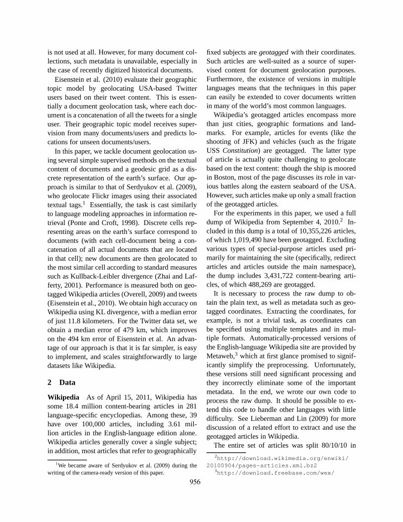
grid size (degrees)

mea

n er

ror

(km

)

0.1 0.5 1 5 10

Most frequent toponymAvg. cell probabilityNaive BayesKullback−Leibler

Figure 1: Plot of grid resolution in degrees versus meanerror for each method on the Wikipedia dev set.

or the same as the title after a parenthetical tag orcomma-separated higher-level division is removed.For example, the toponymTucsonwould match ar-ticles namedTucson, Tucson (city)or Tucson, Ari-zona. In this fashion, the set of toponyms, and thelist of candidates for each toponym, is generatedfrom the set of all geotagged Wikipedia articles.

5 Experiments

The approaches described in the previous sectionare evaluated on both the geotagged Wikipedia andTwitter datasets. Given a predicted cellc for a docu-ment, the prediction error is the great-circle distancebetween the true location and the center ofc, as de-scribed in section 3.

Grid resolution and thresholding The major pa-rameter of all our methods is the grid resolution.For both Wikipedia and Twitter, preliminary ex-periments on the development set were run to plotthe prediction error for each method for each levelof resolution, and the optimal resolution for eachmethod was chosen for obtaining test results. For theTwitter dataset, an additional parameter is a thresh-old on the number of feeds each word occurs in: inthe preprocessed splits of Eisenstein et al. (2010), allvocabulary items that appear in fewer than 40 feedsare ignored. This thresholding takes away a lot ofvery useful material; e.g. in the first feed, it removes

960

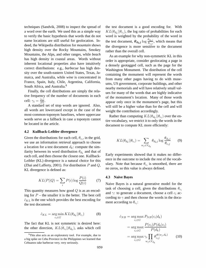
Figure 2: Histograms of distribution of error distances (inkm) for grid size 0.5◦ for each method on the Wikipediadev set.

both “kirkland” and “redmond” (towns in the East-side of Lake Washington near Seattle), very usefulinformation for geolocating that user. This suggeststhat a lower threshold would be better, and this isborne out by our experiments.

Figure 1 graphs the mean error of each method fordifferent resolutions on the Wikipedia dev set, andFigure 2 graphs the distribution of error distancesfor grid size 0.5◦ for each method on the Wikipediadev set. These results indicate that a grid size evensmaller than 0.1◦ might be beneficial. To test this,we ran experiments using a grid size of 0.05◦ and0.01◦ using KL divergence. The mean errors on thedev set increased slightly, from 323 km to 348 and329 km, respectively, indicating that 0.1◦ is indeedthe minimum.

For the Twitter dataset, we considered both gridsize and vocabulary threshold. We recomputed thedistributions using several values for both parame-ters and evaluated on the development set. Table 1shows mean prediction error using KL divergence,for various combinations of threshold and grid size.Similar tables were constructed for the other strate-gies. Clearly, the larger grid size of 5◦ is more op-timal than the 0.1◦ best for Wikipedia. This is un-surprising, given the small size of the corpus. Over-all, there is a less clear trend for the other methods

Grid size (degrees)Thr. 0.1 0.5 1 5 10

0 1113.1 996.8 1005.1 969.3 1052.52 1018.5 959.5 944.6 911.2 1021.63 1027.6 940.8 954.0 913.6 1026.25 1011.7 951.0 954.2 892.0 1013.0

10 1011.3 968.8 938.5 929.8 1048.020 1032.5 987.3 966.0 940.0 1070.140 1080.8 1031.5 998.6 981.8 1127.8

Table 1: Mean prediction error (km) on the Twitter devset for various combinations of vocabulary threshold (infeeds) and grid size, using the KL divergence strategy.

in terms of optimal resolution. Our interpretationof this is that there is greater sparsity for the Twit-ter dataset, and thus it is more sensitive to arbitraryaspects of how different user feeds are captured indifferent cells at different granularities.

For the non-baseline strategies, a threshold be-tween about 2 and 5 was best, although no one valuein this range was clearly better than another.

Results Based on the optimal resolutions for eachmethod, Table 2 provides the median and mean er-rors of the methods for both datasets, when run onthe test sets. The results clearly show that KL di-vergence does the best of all the methods consid-ered, with Naive Bayes a close second. Predictionon Wikipedia is very good, with a median value of11.8 km. Error on Twitter is much higher at 479 km.Nonetheless, this beats Eisenstein et al.’s (2010) me-dian results, though our mean is worse at 967. Us-ing the same threshold of 40 as Eisenstein et al., ourresults using KL divergence are slightly worse thantheirs: median error of 516 km and mean of 986 km.

The difference between Wikipedia and Twitter isunsurprising for several reasons. Wikipedia articlestend to use a lot of toponyms and words that corre-late strongly with particular places while many, per-haps most, tweets discuss quotidian details such aswhat the user ate for lunch. Second, Wikipedia arti-cles are generally longer and thus provide more textto base predictions on. Finally, there are orders ofmagnitude more training examples for Wikipedia,which allows for greater grid resolution and thusmore precise location predictions.

961

Wikipedia TwitterStrategy Degree Median Mean Threshold Degree Median MeanKullback-Leibler 0.1 11.8 221 5 5 479 967Naive Bayes 0.1 15.5 314 5 5 528 989Avg. cell probability 0.1 24.1 1421 2 10 659 1184Most frequent toponym 0.5 136 1927 - - - -Cell prior maximum 5 2333 4309 N/A 0.1 726 1141Random 0.1 7259 7192 20 0.1 1217 1588Eisenstein et al. - - - 40 N/A 494 900

Table 2: Prediction error (km) on the Wikipedia and Twitter test sets for each of the strategies using the optimal gridresolution and (for Twitter) the optimal threshold, as determined by performance on the corresponding developmentsets. Eisenstein et al. (2010) used a fixed Twitter thresholdof 40. Threshold makes no difference for cell priormaximum.

Ships One of the most difficult types of Wikipediapages to disambiguate are those of ships that eitherare stored or had sunk at a particular location. Thesearticles tend to discuss the exploits of these ships,not their final resting places. Location error on theseis usually quite large. However, prediction is quitegood for ships that were sunk in particular battleswhich are described in detail on the page; examplesare the USSGambier Bay, USS Hammann(DD-412), and the HMSMajestic(1895). Another situa-tion that gives good results is when a ship is retiredin a location where it is a prominent feature and isthus mentioned in the training set at that location.An example is the USSTurner Joy, which is in Bre-merton, Washington and figures prominently in thepage for Bremerton (which is in the training set).

Another interesting aspect of geolocating ship ar-ticles is that ships tend to end up sunk in remote bat-tle locations, such that their article is the only onelocated in the cell covering the location in the train-ing set. Ship terminology thus dominates such cells,with the effect that our models often (incorrectly)geolocate test articles about other ships to such loca-tions (and often about ships with similar properties).This also leads to generally more accurate geoloca-tion of HMS ships over USS ships; the former seemto have been sunk in more concentrated regions thatare themselves less spread out globally.

6 Related work

Lieberman and Lin (2009) also work with geotaggedWikipedia articles, but they do in order so to ana-

lyze the likely locations of users who edit such ar-ticles. Other researchers have investigated the useof Wikipedia as a source of data for other super-vised NLP tasks. Mihalcea and colleagues have in-vestigated the use of Wikipedia in conjunction withword sense disambiguation (Mihalcea, 2007), key-word extraction and linking (Mihalcea and Csomai,2007) and topic identification (Coursey et al., 2009;Coursey and Mihalcea, 2009). Cucerzan (2007)used Wikipedia to do named entity disambiguation,i.e. identification and coreferencing of named enti-ties by linking them to the Wikipedia article describ-ing the entity.

Some approaches to document geolocation relylargely or entirely on non-textual metadata, whichis often unavailable for many corpora of interest,Nonetheless, our methods could be combined withsuch methods when such metadata is available. Forexample, given that both Wikipedia and Twitter havea linked structure between documents, it would bepossible to use the link-based method given in Back-strom et al. (2010) for predicting the location ofFacebook users based on their friends’ locations. Itis possible that combining their approach with ourtext-based approach would provide improvementsfor Facebook, Twitter and Wikipedia datasets. Forexample, their method performs poorly for userswith few geolocated friends, but results improvedby combining link-based predictions with IP addresspredictions. The text written users’ updates could bean additional aid for locating such users.

962

7 Conclusion

We have shown that automatic identification of thelocation of a document based only on its text can beperformed with high accuracy using simple super-vised methods and a discrete grid representation ofthe earth’s surface. All of our methods are simpleto implement, and both training and testing can beeasily parallelized. Our most effective geolocationstrategy finds the grid cell whose word distributionhas the smallest KL divergence from that of the testdocument, and easily beats several effective base-lines. We predict the location of Wikipedia pagesto a median error of 11.8 km and mean error of 221km. For Twitter, we obtain a median error of 479km and mean error of 967 km. Using naive Bayesand a simple averaging of word-level cell distribu-tions also both worked well; however, KL was moreeffective, we believe, because it weights the wordsin the document most heavily, and thus puts less im-portance on the less specific word distributions ofeach cell.

Though we only use text, link-based predictionsusing the follower graph, as Backstrom et al. (2010)do for Facebook, could improve results on the Twit-ter task considered here. It could also help withWikipedia, especially for buildings: for example,the page for Independence Hall in Philadelphia linksto geotagged “friend” pages for Philadelphia, theLiberty Bell, and many other nearby locations andbuildings. However, we note that we are still pri-marily interested in geolocation with only text be-cause there are a great many situations in which suchlinked structure is unavailable. This is especiallytrue for historical corpora like those made availableby the Perseus project.9

The task of identifying a single location for an en-tire document provides a convenient way of evaluat-ing approaches for connecting texts with locations,but it is not fully coherent in the context of docu-ments that cover multiple locations. Nonetheless,both the average cell probability and naive Bayesmodels output a distribution over all cells, whichcould be used to assign multiple locations. Further-more, these cell distributions could additionally beused to define a document level prior for resolutionof individual toponyms.

9www.perseus.tufts.edu/

Though we treated the grid resolution as a param-eter, the grids themselves form a hierarchy of cellscontaining finer-grained cells. Given this, there area number of obvious ways to combine predictionsfrom different resolutions. For example, given a cellof the finest grain, the average cell probability andnaive Bayes models could successively back off tothe values produced by their coarser-grained con-taining cells, and KL divergence could be summedfrom finest-to-coarsest grain. Another strategy formaking models less sensitive to grid resolution is tosmooth the per-cell word distributions over neigh-boring cells; this strategy improved results on Flickrphoto geolocation for Serdyukov et al. (2009).

An additional area to explore is to remove thebag-of-words assumption and take into account theordering between words. This should have a num-ber of obvious benefits, among which are sensitivityto multi-word toponyms such asNew York, colloca-tions such asLondon, Ontarioor London in Ontario,and highly indicative terms such asegg creamthatare made up of generic constituents.

Acknowledgments

This research was supported by a grant from theMorris Memorial Trust Fund of the New York Com-munity Trust and from the Longhorn InnovationFund for Technology. This paper benefited from re-viewer comments and from discussion in the Natu-ral Language Learning reading group at UT Austin,with particular thanks to Matt Lease.

References

Geoffrey Andogah. 2010.Geographically ConstrainedInformation Retrieval. Ph.D. thesis, University ofGroningen, Groningen, Netherlands, May.

Lars Backstrom, Eric Sun, and Cameron Marlow. 2010.Find me if you can: improving geographical predictionwith social and spatial proximity. InProceedings ofthe 19th international conference on World wide web,WWW ’10, pages 61–70, New York, NY, USA. ACM.

Kino Coursey and Rada Mihalcea. 2009. Topic identi-fication using wikipedia graph centrality. InProceed-ings of Human Language Technologies: The 2009 An-nual Conference of the North American Chapter of theAssociation for Computational Linguistics, Compan-ion Volume: Short Papers, NAACL ’09, pages 117–

963

120, Morristown, NJ, USA. Association for Computa-tional Linguistics.

Kino Coursey, Rada Mihalcea, and William Moen. 2009.Using encyclopedic knowledge for automatic topicidentification. InProceedings of the Thirteenth Con-ference on Computational Natural Language Learn-ing, CoNLL ’09, pages 210–218, Morristown, NJ,USA. Association for Computational Linguistics.

Silviu Cucerzan. 2007. Large-scale named entity dis-ambiguation based on Wikipedia data. InProceedingsof the 2007 Joint Conference on Empirical Methodsin Natural Language Processing and ComputationalNatural Language Learning (EMNLP-CoNLL), pages708–716, Prague, Czech Republic, June. Associationfor Computational Linguistics.

Junyan Ding, Luis Gravano, and Narayanan Shivaku-mar. 2000. Computing geographical scopes of web re-sources. InProceedings of the 26th International Con-ference on Very Large Data Bases, VLDB ’00, pages545–556, San Francisco, CA, USA. Morgan Kauf-mann Publishers Inc.

G. Dutton. 1996. Encoding and handling geospatial datawith hierarchical triangular meshes. In M.J. Kraak andM. Molenaar, editors,Advances in GIS Research II,pages 505–518, London. Taylor and Francis.

Jacob Eisenstein, Brendan O’Connor, Noah A. Smith,and Eric P. Xing. 2010. A latent variable modelfor geographic lexical variation. InProceedings ofthe 2010 Conference on Empirical Methods in NaturalLanguage Processing, pages 1277–1287, Cambridge,MA, October. Association for Computational Linguis-tics.

Qiang Hao, Rui Cai, Changhu Wang, Rong Xiao, Jiang-Ming Yang, Yanwei Pang, and Lei Zhang. 2010.Equip tourists with knowledge mined from travel-ogues. InProceedings of the 19th international con-ference on World wide web, WWW ’10, pages 401–410, New York, NY, USA. ACM.

Jochen L. Leidner. 2008.Toponym Resolution in Text:Annotation, Evaluation and Applications of SpatialGrounding of Place Names. Dissertation.Com, Jan-uary.

M. D. Lieberman and J. Lin. 2009. You are where youedit: Locating Wikipedia users through edit histories.In ICWSM’09: Proceedings of the 3rd InternationalAAAI Conference on Weblogs and Social Media, pages106–113, San Jose, CA, May.

Bruno Martins. 2009.Geographically Aware Web TextMining. Ph.D. thesis, University of Lisbon.

Rada Mihalcea and Andras Csomai. 2007. Wikify!: link-ing documents to encyclopedic knowledge. InPro-ceedings of the sixteenth ACM conference on Con-ference on information and knowledge management,

CIKM ’07, pages 233–242, New York, NY, USA.ACM.

Rada Mihalcea. 2007. Using Wikipedia for Auto-matic Word Sense Disambiguation. InNorth Ameri-can Chapter of the Association for Computational Lin-guistics (NAACL 2007).

Simon Overell. 2009. Geographic Information Re-trieval: Classification, Disambiguation and Mod-elling. Ph.D. thesis, Imperial College London.

Jay M. Ponte and W. Bruce Croft. 1998. A languagemodeling approach to information retrieval. InPro-ceedings of the 21st annual international ACM SIGIRconference on Research and development in informa-tion retrieval, SIGIR ’98, pages 275–281, New York,NY, USA. ACM.

Erik Rauch, Michael Bukatin, and Kenneth Baker. 2003.A confidence-based framework for disambiguating ge-ographic terms. InProceedings of the HLT-NAACL2003 workshop on Analysis of geographic references- Volume 1, HLT-NAACL-GEOREF ’03, pages 50–54,Stroudsburg, PA, USA. Association for ComputationalLinguistics.

Bjorn Sandvik. 2008. Using KML for thematic mapping.Master’s thesis, The University of Edinburgh.

Pavel Serdyukov, Vanessa Murdock, and Roelof vanZwol. 2009. Placing flickr photos on a map. InPro-ceedings of the 32nd international ACM SIGIR con-ference on Research and development in informationretrieval, SIGIR ’09, pages 484–491, New York, NY,USA. ACM.

David A. Smith and Gregory Crane. 2001. Disam-biguating geographic names in a historical digital li-brary. In Proceedings of the 5th European Confer-ence on Research and Advanced Technology for Digi-tal Libraries, ECDL ’01, pages 127–136, London, UK.Springer-Verlag.

B. E. Teitler, M. D. Lieberman, D. Panozzo, J. Sankara-narayanan, H. Samet, and J. Sperling. 2008. News-Stand: A new view on news. InGIS’08: Proceedingsof the 16th ACM SIGSPATIAL International Confer-ence on Advances in Geographic Information Systems,pages 144–153, Irvine, CA, November.

Chengxiang Zhai and John Lafferty. 2001. Model-basedfeedback in the language modeling approach to infor-mation retrieval. InProceedings of the tenth interna-tional conference on Information and knowledge man-agement, CIKM ’01, pages 403–410, New York, NY,USA. ACM.

964