quasilocal contribution to the scalar self-force: geodesic motion
TRANSCRIPT
arX
iv:0
711.
2469
v3 [
gr-q
c] 5
May
200
8
Quasi-local contribution to the scalar self-force: Geodesic Motion
Adrian C. Ottewill∗ and Barry Wardell†
School of Mathematical Sciences, University College Dublin, Belfield, Dublin 4, Ireland
(Dated: May 5, 2008)
We consider a scalar charge travelling in a curved background spacetime. We calculate the quasi-local contribution to the scalar self-force experienced by such a particle following a geodesic in ageneral spacetime. We also show that if we assume a massless field and a vacuum backgroundspacetime, the expression for the self-force simplifies significantly. We consider some specific caseswhose gravitational analog are of immediate physical interest for the calculation of radiation reactioncorrected orbits of binary black hole systems. These systems are expected to be detectable by theLISA space based gravitational wave observatory. We also investigate how alternate techniques maybe employed in some specific cases and use these as a check on our own results.
I. INTRODUCTION
There has been considerable recent interest in the modelling of astronomical and cosmological gravitational wavesources. This interest has been spurred on by the recent and upcoming construction of both ground and space basedgravitational wave observatories. Ground based detectors such as LIGO [1], VIRGO [2] and GEO600 [3] have alreadyreached the data collection phase. The primary space based gravitational wave observatory, LISA [4] - the LaserInterferometer Space Antenna - is still in the design and planning phase. A joint NASA/ESA mission, it is expectedto launch within the next few years. It will detect gravitational waves in the frequency band 0.1-0.0001Hz, a band inwhich a considerable number of interesting gravitational wave sources are expected to be found.
In order to extract the maximum amount of information from these gravitational wave detectors, data analysistechniques such as matched filtering may be employed. To improve the effectiveness of this data analysis, it isnecessary to have accurate predictions of the waveforms of the gravitational radiation emitted by candidate sources.One of the primary candidate sources of such a gravitational wave signal falls under the category of large mass binarysystems. In particular, extreme mass ratio systems such as that of a compact solar mass object (mass m) inspirallinginto a black hole of 103 to 108 solar masses (mass M) are expected to be detectable by LISA out to Gpc distances.
As a prerequisite to the calculation of the waveform templates for such sources, it is necessary to model the orbitalevolution of the system. In the case of extreme mass ratio systems, we can do so by making the approximation thatthe smaller mass is travelling in the background spacetime of the larger mass. However, the compact nature of thesmaller mass means that it itself will distort the curvature of the spacetime in which it is moving to a non-negligibleextent. As a result, it does not follow a geodesic of the background spacetime of the larger mass, but rather, it followsa geodesic of the total spacetime of both masses. In this sense the motion of the smaller mass is affected by thepresence of its own mass, i.e. the smaller mass is seen to exert a force on itself. This is called the self-force. Clearly,the computation of this self-force is of fundamental importance to the accurate calculation of the orbital evolution ofsuch binary systems and hence to the prediction of the gravitational radiation waveform.
Because of this non-linear behavior, it is extremely difficult, if not impossible, to exactly solve the equations ofmotion of such a system. However, due to the extreme mass ratio involved, the deviation of the object’s trajectoryfrom the background geodesic is small over sufficiently small time-scales (less than the natural length-scale of thebackground). In this case, to linear order in m, we can model the deviation from the background as a spin-2 fieldgenerated by the particle and living on the background spacetime. This field is then seen to couple to the smallerobject to cause the self-force.
In the present work, we will focus not on the gravitational self-force described thus far, but rather on the analogousbut simpler scalar self-force. Instead of considering the smaller mass, m, to be generating a gravitational field, wetake it to have a scalar charge, q. This charge couples to a massless scalar field which is then the cause of the self-force. Otherwise, we leave the problem exactly as posed above. In making this change, the resulting analysis remainsextremely similar to the gravitational case, but the algebraic details of the calculations become simpler. This willallow us to explore the problem and develop techniques which we will at a later date apply to the physically moreinteresting gravitational case.
∗Electronic address: [email protected]†Electronic address: [email protected]
2
An expression for the electromagnetic self-force was originally obtained by DeWitt and Brehme [5] (later correctedby Hobbs [6]) and more recently recovered by Quinn and Wald [7]. In addition, Ref. [7] derives an expression for thegravitational self-force, as was done previously by Mino, Sasaki and Tanaka [8]. Using a generalization of his axiomaticapproach, Quinn also obtained an expression for the scalar self-force [9]. These results show how the self-force may beexpressed in terms of an integral of the retarded Green’s function over the entire past world-line of the particle. Thisretarded Green’s function possesses two terms, one representing geodesic propagation, the other a tail-term arisingfrom back-scattering by the spacetime geometry. (Solutions to wave equations on most curved manifolds depend notonly on Cauchy data directly intersecting the past light cone, but also on Cauchy data interior to that intersection.The portion of the field that propagates in the null directions is called the direct part, while the portion of the fieldthat propagates in the timelike directions inside the light cone is called the tail.) Clearly, the tail part of a particle’sfield can interact with the particle, leading to a contribution to the self-force.
Although in principle this formal solution gives the desired result, in practice the calculation of the Green’s functionposes a formidable challenge. There has been a significant amount of work in this area in recent years. Varioustechniques have been employed. There has been considerable recent success using mode-sum approaches, amongstothers [10, 11, 12, 13, 14]. Other work has focused on a matched expansion approach and also on obtaining exactsolutions under specific circumstances. For the Schwarzschild background, Wiseman [15] found an exact solution forthe scalar self-force on a particle held at rest. Anderson, Hu and Eftekharzadeh [16] built on this work along withother results to derive an expression for the self-force on a particle held at rest, then released and allowed to fallradially inward. Anderson and Wiseman [17] also examined the matched expansion approach under the two casesof static particles and circular geodesic paths in a Schwarzschild background. For the case of a gravitational field,Anderson, Flanagan and Ottewill [18] have evaluated the quasi-local contribution to the self-force up to O
(
∆τ3)
.Comprehensive reviews of the radiation-reaction and self-force problem are given by Poisson [19] and by Detweiler[20].
In this paper, we use the results of Decanini and Folacci [22] as a basis for our own work. In section II we firstrecap the work of Quinn [9] to define what we mean by the quasi-local part of the self-force and then we derive anexpression for it and for the equations of motion in terms of the Green’s function. Next, in section III we use thisresult to calculate an expression for the quasi-local portion of the scalar self-force in terms of the expansion coefficientsgiven by Ref. [22], and in terms of the proper time to the matching point ∆τ and the 4-velocity of the particle, uα.
By making the assumption of motion in a massless field on a vacuum background spacetime, we show in section IVthat the resulting self-force expression simplifies considerably and in fact vanishes up to and including third order in∆τ .
In section V, we examine some particularly interesting and simple cases in both Schwarzschild and Kerr spacetimes.We then show that using a corrected form of the results of Ref. [17], we obtain identical results, order by order forthese special cases. This confirms the consistency of our results and the validity of our approach. We also presentcorrected results for the higher order terms in Ref. [17] and give updated truncation error graphs.
Throughout this paper, we use units in which G = c = 1 and adopt the sign conventions of [23]. We denotesymmetrization of indices using brackets (e.g. (αβ)) and exclude indices from symmetrization by surrounding themby vertical bars (e.g. (α|β|γ)). Roman letters are used for free indices and Greek letters for indices summed over allspacetime dimensions.
II. THE QUASI-LOCAL SCALAR SELF-FORCE AND EQUATIONS OF MOTION
Consider a particle of scalar charge q and mass m travelling in a curved background spacetime. We treat this asa point particle and will refer to it as a particle throughout this paper. However, the arguments presented here areequally valid for non-point objects provided the object’s extended structure does not affect its center-of-mass motion.
The scalar field generated by the particle propagates along null geodesics, while the particle itself will (approxi-mately) follow a time-like geodesic of the background. The field then interacts with the particle, effectively causing aforce, called the scalar self-force. This self-force may be expressed as a sum of local and non-local parts [9]
fa = q2
(
1
3
(
aa − a2ua)
+1
6
(
Raβuβ + Rβγuβuγua)
+
(
1
2m2
field −1
12(1 − 6ξ)R
)
ua
)
+limǫ→0
q2
∫ τ−ǫ
−∞
∇aGret (x, x′) dτ ′
(2.1)where uα is the 4-velocity of the particle, a is the 4-acceleration, a = ∂a
∂τ is the derivative of the 4-acceleration withrespect to proper time and Gret is the retarded scalar Green’s function. Here, we have trivially extended the expressiongiven in Ref. [9] and Ref. [19] to include terms corresponding to the field mass mfield and coupling to the backgroundscalar curvature, ξ.
3
In this form, the local terms are all given explicitly, so their calculation can be carried out immediately withoutposing any real difficulty. Our task is therefore to elucidate the non-local integral term. To this end, we will workwith an expression for the self-force which just contains the non-local integral term:
fa = limǫ→0
q2
∫ τ−ǫ
−∞
∇aGret (x, x′) dτ ′ (2.2)
We do so with the understanding that the local terms can easily be added back in later if necessary.This leaves us with an expression for the scalar self-force in terms of an integral of the gradient of the retarded
Green’s function over the entire past world line of the particle. The limiting feature at the upper limit of integrationis necessary because of the singular nature of the Green’s function at the point x = x′.
This integral would normally be evaluated using a mode-sum approach. One would calculate a sufficient number ofthe modes and sum them up to obtain the Green’s function solution and hence the self-force. However, the limitingfeature in the upper limit of integration causes great difficulties for this method. As ǫ decreases, it is necessary totake an increasing number of modes to obtain an accurate solution. When ǫ tends towards 0, the number of modesrequired becomes infinite and it is no longer possible to accurately compute the integral. However, we can avoid thisproblem if we split the integral in two parts
fa = limǫ→0
q2
∫ τ−ǫ
τ−∆τ
∇aGret (x, x′) dτ ′ + q2
∫ τ−∆τ
−∞
∇aGret (x, x′) dτ ′ (2.3)
where τ − ∆τ is a matching point. It is chosen so that both integrals may be evaluated separately using differentmeans and then combined to obtain an expression for the total self-force. The second integral in this expressionmay be evaluated, for example, by using the methods of quantum field theory in curved spacetime [24] to perform amode-sum calculation of the Green’s function away from the singularity x = x′. We call the first term in Eq. (2.3)the quasi-local part of the self-force. It is the computation of this integral that is the main focus of the remainder ofthis paper.
The greatest obstacle to obtaining a solution for this quasi-local integral lies with the difficulty in the computationof the retarded Green’s function, Gret. It is a solution of the wave equation on a curved background spacetime:
(
�x − m2 − ξR)
Gret (x, x′) = −4πδ (x, x′) (2.4)
In general, it proves extremely difficult, if not impossible, to find an exact solution of Eq. (2.4). However, providedx and x′ are sufficiently close, we can use the Hadamard form for the retarded Green’s function solution [9],
Gret (x, x′) = θ− (x, x′) {U (x, x′) δ (σ (x, x′)) − V (x, x′) θ (−σ (x, x′))} (2.5)
where θ− (x, x′) is analogous to the Heaviside step-function (i.e. 1 when x′ is in the causal past of x, 0 otherwise),δ (x, x′) is the standard Dirac delta function, U (x, x′) and V (x, x′) are symmetric bi-scalars having the benefit thatthey are regular for x′ → x and σ (x, x′) is the Synge [19, 21, 25] world function. For the time-like geodesics that areof interest to this paper, σ is equal to minus one half of the squared geodesic distance between x and x′:
σ (x, x′) = −1
2s2 (2.6)
This form of the retarded Green’s function is valid provided x′ lies within a normal neighborhood of x, i.e. providedthere is a unique geodesic connecting x and x′. Clearly, by simply choosing an appropriate value for ∆τ , we cansatisfy this normal neighborhood condition and use the Hadamard form for the retarded Green’s function in the firstintegral in Eq. (2.3).1
The first term (involving U (x, x′)) in Eq. (2.5) is called the direct part of the Green’s function and does notcontribute to the self-force. This can be understood by the fact that the presence of δ (σ (x, x′)) in the direct part ofGret means that it is only non-zero on the past light-cone of the particle. However, since the quasi-local integral inEq. (2.3) is totally internal to the past light-cone, this term does not contribute to the integral.
The second term in Eq. (2.5) is known as the tail part of the Green’s function. It is this term that is responsiblefor the self-force and its calculation is the primary focus of this paper.
1 Anderson and Wiseman [17] have calculated some explicit values for the normal neighborhood boundary for a particle following a circulargeodesic in Schwarzschild spacetime. These values place an upper bound estimation on the geodesic distance in the past at which wecan place the matching point ∆τ .
4
We can now substitute Eq. (2.5) into the quasi-local part of Eq. (2.3) to obtain the final form of the quasi-localself-force:
faQL = −q2
∫ τ
τ−∆τ
∇aV (x, x′) dτ ′ (2.7)
Note that it is no longer necessary to take the limit since V (x, x′) is regular everywhere.Unlike the cases of electromagnetic and gravitational fields, where the 4-acceleration is exactly equal to the self-force
divided by the mass, there is one further step required in order to obtain the equations of motion in the presence of ascalar field. In this case, the self-force contains two components, one related to the 4-acceleration, the other relatedto the change in mass:
faQL =
dm
dτua + maa (2.8)
The 4-acceleration is always orthogonal to the 4-velocity, so in order to obtain it from the self-force, we take theprojection of fa orthogonal to ua:
maa = P aβ fβ (2.9)
where
P ba = δb
a + uaub (2.10)
is the projection orthogonal to uα.The remaining component of the self-force (which is tangent to the 4-velocity) is simply the change in mass:
dm
dτ= −fαuα (2.11)
III. COVARIANT CALCULATION
Within the Hadamard approach, the symmetric bi-scalar V (x, x′) is expressed in terms of an expansion in increasingpowers of σ [22]:
V (x, x′) =
∞∑
n=0
Vn (x, x′)σn (x, x′) (3.1)
Substituting the expansion (3.1) into Eq. (2.4), using the identity σ;ασ;α = 2σ and explicitly setting the coefficient ofeach manifest power of σn equal to zero, we find (in 4-dimensional space-time) that the coefficients Vn (x, x′) satisfythe recursion relations
(n + 1) (2n + 4)Vn+1 + 2 (n + 1)Vn+1;µσ;µ − 2 (n + 1)Vn+1∆−1/2∆
1/2;µσ;µ +
(
�x − m2 − ξR)
Vn = 0 for n ∈ N
(3.2)along with the initial conditions
2V0 + 2V0;µσ;µ − 2V0∆−1/2∆
1/2;µσ;µ +
(
�x − m2 − ξR)
U0 = 0 (3.3a)
U0 = ∆1/2 (3.3b)
The quantity ∆ (x, x′) is the Van Vleck-Morette determinant defined as [22]
∆ (x, x′) = − [−g (x)]−1/2
det (−σ;µν′ (x, x′)) [−g (x′)]−1/2
(3.4)
It is important to note that the Hadamard expansion is not a Taylor series and is not unique. Indeed, in Appendix Bwe show how, under the assumption of a massless field on a vacuum background spacetime, the terms from V0 and V1
5
conspire to cancel to third order when combined to form V . Such cancellation is also seen, for example, in deSitterspace-time, where for a conformally invariant theory all the Vn’s are non-zero while V ≡ 0.
In order to solve the recursion relations (3.2) and (3.3) for the coefficients Vn (x, x′), it is convenient to first writeVn (x, x′) in terms of its covariant Taylor series expansion about x = x′:
Vn (x, x′) =
∞∑
p=0
(−1)p
p!vn(p) (x, x′) (3.5)
where the vn(p) are bi-scalars of the form
vn(p) (x, x′) = vn α1...αp(x)σ;α1 (x, x′) . . . σ;αp (x, x′) (3.6)
Decanini and Folacci [22] calculated expressions for these vn(p) up to O(
σ2)
, or equivalently O(
∆τ4)
, where ∆τ isthe magnitude of the proper time separation between x and x′. In Appendix A, we use the symmetry of the Green’sfunction in x and x′ to extend their results by one order in the proper time separation, ∆τ , or equivalently one halforder in σ (x, x′).
We now turn to the evaluation of the self-force. We could calculate the self-force given this form for Vn (x, x′),however, it proves easier to work with V (x, x′) expressed in the form of a covariant Taylor expansion, i.e. an expansionin increasing powers of σ;a:
V (x, x′) =
∞∑
p=0
(−1)p
p!vα1...αp
(x)σ;α1 (x, x′) . . . σ;αp (x, x′) (3.7)
Explicit expressions for the va1...ap(x), up to O
(
σ5/2)
, can then be easily obtained order by order by combining therelevant vn a1...ap
as described in Appendix B.Substituting Eq. (3.7) into Eq. (2.7), taking the covariant derivative and noting that the va1...ap
are symmetricunder exchange of all indices, a1, . . . , ap, we obtain an expression for the self-force in terms of va1...ap
, σ and theirderivatives:
faQL = −q2
∫ τ
τ−∆τ
[
v;a − v ;aβ σ;β − vβσ;βa +
2
2!vβγσ;βaσ;γ +
1
2v ;a
βγ σ;βσ;γ −3
3!vβγδσ
;βaσ;γσ;δ
−1
3!v ;a
βγδ σ;βσ;γσ;δ +4
4!vβγδǫσ
;βaσ;γσ;δσ;ǫ +1
4!v ;a
βγδǫ σ;βσ;γσ;δσ;ǫ
−5
5!vβγδǫζσ
;βaσ;γσ;δσ;ǫσ;ζ + O(
σ5/2) ]
dτ ′ (3.8)
Now, by definition, for a time-like geodesic,
σ = −1
2(τ − τ ′)
2(3.9a)
σ;a = − (τ − τ ′)ua (3.9b)
where ua is the 4-velocity of the particle.Also, the quantity σ;ab can be written in terms of a covariant Taylor series expansion [5, 19, 22]:
σ;ab = gab −1
3Ra b
α βσ;ασ;β +1
12Ra b
α β;γσ;ασ;βσ;γ −
[
1
60Ra b
α β;γδ +1
45Ra
αρβRρ bγ δ
]
σ;ασ;βσ;γσ;δ + O(
(σ;a)5)
(3.10)
Substituting Eqs. (3.9a), (3.9b) and (3.10) into Eq. (3.8), the integrand becomes an expansion in powers of theproper time, τ − τ ′:
faQL = −q2
∫ τ
τ−∆τ
[
Aa(τ − τ ′)0
+ Ba(τ − τ ′)1+ Ca(τ − τ ′)
2
+ Da(τ − τ ′)3
+ Ea(τ − τ ′)4
+ O(
(τ − τ ′)5) ]
dτ ′ (3.11)
6
where
Aa = v;a − vβgβa (3.12a)
Ba = v ;aβ uβ − vβγgβauγ (3.12b)
Ca =1
3vβRβ a
γ δuγuδ +
1
2v ;a
βγ uβuγ −1
2vβγδg
βauγuδ (3.12c)
Da =1
12vβRβ a
γ δ;ǫuγuδuǫ +
1
3vβγRβ a
δ ǫuγuδuǫ +
1
6v ;a
βγδ uβuγuδ −1
6vβγδǫg
βauγuδuǫ (3.12d)
Ea = vβ
(
1
60Rβ a
γ δ;ǫζ +1
45Rβ
γρδRρ aǫ ζ
)
uγuδuǫuζ +1
12vβγRβ a
δ ǫ;ζuγuδuǫuζ
+1
6vβγδR
β aǫ ζu
γuδuǫuζ +1
24v ;a
βγδǫ uβuγuδuǫ −1
24vβγδǫζg
βauγuδuǫuζ (3.12e)
The coefficients of the powers of τ − τ ′ are all local quantities at x, but the integral is in terms of the primedcoordinates, x′, so the coefficients may be treated as constants while performing the integration. The result is thatwe only have to perform a trivial integral of powers of τ − τ ′. Performing the integration gives us our final result, thequasi-local part of the self force in terms of an expansion in powers of the matching point, ∆τ :
faQL = −q2
(
Aa∆τ1 +1
2Ba∆τ2 +
1
3Ca∆τ3 +
1
4Da∆τ4 +
1
5Ea∆τ5 + O
(
∆τ6)
)
(3.13)
It is possible to simplify Eqs. (3.12a) - (3.12e) further by using the results of Appendix A to rewrite all the oddorder va1...ap
terms in terms of the lower order even terms. It is then straightforward to substitute in for the va1...ap
to get an expression for the quasi-local self-force in terms of only the scalar charge, field mass, coupling to the scalarbackground, 4-velocity, and products of Riemann tensor components of the background spacetime. However, wechoose not to do so here as that would result in excessively lengthy expressions. Instead, we direct the reader to Ref.[22] for a general expression for the vna1...ap
for a scalar field and to Appendix B where we give the expressions forthe vna1...ap
for massless scalar fields in vacuum spacetimes up to the orders required.Once an expression has been obtained for the self-force using this method, it is straightforward to use Eqs. (2.9) -
(2.11) to obtain the equations of motion.
IV. SIMPLIFICATION OF THE QUASI-LOCAL SELF-FORCE FOR MASSLESS FIELDS IN VACUUMSPACE-TIMES
Eq. (3.13) is valid for any geodesic motion in any scalar field (massless or massive) in any background spacetime.At first it may appear that this result is quite difficult to work with due to the length of the expressions given in Ref.[22] for the vna1...ap
. However, if we make the two assumptions that:
1. The scalar field is massless (mfield = 0)
2. The background spacetime is a vacuum spacetime (Rαβ = 0)
the majority of these terms vanish and we are left with the much more manageable expressions for the vna1...apgiven
in Appendix B.In Appendix B, we give the expansion coefficients vna1...ap
up to O(
σ5/2)
for a massless field in a vacuum space-time. We can see immediately from these expressions that all terms involving vα, vαβ and vαβγ identically vanish.That leaves expressions involving only vαβγδ and vαβγδǫ. However, Eq. (A1) gives us a relation which allows us toexpress any odd order term (in this case, vαβγδζ) in terms of all the lower order terms. This, along with the fact thatva1...ap
is totally symmetric, leads to a vastly simplified expression for the quasi-local self-force on a scalar particlefollowing a geodesic in a vacuum background spacetime:
faQL = q2
(
1
4!vβγδǫg
βauγuδuǫ∆τ4 −1
5!
(
1
2vγδǫζ;β − 2vβγδǫ;ζ
)
gβauγuδuǫuζ∆τ5 + O(
∆τ6)
)
(4.1)
We see that a large number of terms in (3.13) either identically vanish or cancel each other out. In fact, at the firstthree orders in ∆τ , we get no contribution to the quasi-local self-force whatsoever. Additionally, our fourth and fifthorder coefficients take on a much simpler form than the general case given in Eqs. (3.12d) and (3.12e).
7
V. SOME SPECIAL CASES
Expression (4.1) is a very general result, giving the quasi-local part of the self-force on a scalar charge followingan arbitrary time-like geodesic in any 4-dimensional vacuum spacetime. While such a general result is of tremendousbenefit in terms of flexibility, it is also interesting to examine some specific cases whose gravitational analog are ofimmediate physical interest. We will consider two well-known black hole spacetimes, Schwarzschild and Kerr, andsome physically probable geodesics paths.
Although these results apply only to the non-physical scalar charge, we envisage that the techniques developed herecould be applied to the more complicated gravitational case. This would allow us to work out the quasi-local part ofthe gravitational self-force. In conjunction with a mode-sum approximation of the far-field part of the integral, wewould then be able to calculate the total self-force. Hence it would be possible to calculate the waveform correspondingto the gravitational radiation emitted from such a system. These waveforms are expected to be of great importancein the detection of gravitational wave sources by LISA [4], the space based gravitational wave observatory .
A. Schwarzschild Space-time
We begin with Schwarzschild spacetime as that is the simpler of the two cases. The line-element of this spacetimeis given by
ds2 =
(
1 −2M
r
)−1
dr2 + r2(
dθ2 + sin2 θdφ2)
−
(
1 −2M
r
)
dt2 (5.1)
From this, we calculate all necessary components of the Riemann tensor and its covariant derivatives and hence valuesfor all the va1...ap
. While the calculations involved pose no conceptual difficulty, there is a great deal of scope fornumerical slips. Fortunately, they are well suited to being done using a computer algebra system such as the GRTensor[26] package for the Maple CAS [27].
We consider a particle with a general geodesic 4-velocity uα travelling in this background spacetime. At first glance,it may appear that there are four independent components of this 4-velocity. However, because of the sphericalsymmetry of the problem, we may arbitrarily choose the orientation of the equatorial axis, θ. By choosing this toline up with the 4-velocity (i.e. θ = π
2 ), we can see immediately that uθ = 0. Furthermore, the particle is followinga time-like geodesic, so the normalization condition on the 4-velocity uαuα = −1 holds. This allows us to eliminateone of the three remaining components. In our case, we choose to eliminate ut, which has the equation:
ut =
√
(
r
r − 2M
) (
1 +r
r − 2M(ur)
2+ r2 (uφ)
2
)
(5.2)
We are now left with just two independent components of the 4-velocity, uφ and ur. Substituting in to Eq. (4.1)the values for the known 4-velocity components uθ and ut along with the Riemann tensor components, we get ageneral expression for the scalar self-force in terms of the scalar charge, q, the matching point, ∆τ , the mass of theSchwarzschild black hole, M , the radial distance of the scalar charge from the black hole, r and the two independentcomponents of the 4-velocity of the scalar charge, ur and uφ. We can then use Eqs. (2.9) - (2.11) to obtain thequasi-local contribution to the equations of motion:
marQL =
3q2M2
11200r10
{
10r2ur
[(
r − 2M
r
)
(
1 + 11(
ruφ)2
+ 13(
ruφ)4
)
+ (ur)2(
1 + 8(
ruφ)2
)
]
∆τ4
−
[
(
r − 2M
r
)
(
(20r − 49M) + 8 (11r − 28M)(
ruφ)2
+ 2 (34r − 89M)(
ruφ)4
)
+ (ur)2(
(4r − 17M) − 8 (31r − 59M)(
ruφ)2
− 30 (14r − 29M)(
ruφ)4
)
− 16r (ur)4(
1 + 15(
ruφ)2
)
]
∆τ5 + O(
∆τ6)
}
(5.3a)
maθQL = O
(
∆τ6)
(5.3b)
8
maφQL =
3q2M2
11200r10uφ
{
10r2
[(
r − 2M
r
)
(
7 + 20(
ruφ)2
− 13(
ruφ)4
)
+ (ur)2(
5 + 8(
ruφ)2
)
]
∆τ4
+ ur
[
3 (68r − 141M) + 48 (13r − 27M)(
ruφ)2
+ 30 (14r − 29M)(
ruφ)4
+ 48r (ur)2(
3 + 5(
ruφ)2
)
]
∆τ5 + O(
∆τ6)
}
(5.3c)
matQL = −
3q2M2
11200r10
√
r
r − 2M
(
1 + (ruφ)2
+r
r − 2M(ur)
2
)
×
{
10r2
[(
r − 2M
r
)
(
7(
ruφ)2
+ 13(
ruφ)4
)
+ (ur)2(
1 + 8(
ruφ)2
)
]
∆τ4
+ ur[
(20r − 49M)− 8 (17r − 31M)(
ruφ)2
− 30 (14r − 29M)(
ruφ)4
− 16r (ur)2(
1 + 15(
ruφ)2
)]
∆τ5
+ O(
∆τ6)
}
(5.3d)
dm
dτ= −
3q2M2
11200r10
{
5r2
[(
r − 2M
r
)
(
5 + 28(
ruφ)2
+ 26(
ruφ)4
)
+ 4 (ur)2(
1 + 4(
ruφ)2
)
]
∆τ4
− 3ur
[
(20r − 41M) + 8 (17r − 35M)(
ruφ)2
+ 10 (14r − 29M)(
ruφ)4
+ 16r (ur)2(
1 + 5(
ruφ)2
)
]
∆τ5
+ O(
∆τ6)
}
(5.3e)
We see that the θ-component of the 4-acceleration is 0 as would be expected for motion in the equatorial plane. We
also find that the other three components, marQL, maφ
QL and matQL all have their leading order terms at O
(
∆τ4)
and
also have terms at order O(
∆τ5)
.We may also express this result in an alternative way by making use of the constants of motion [29]:
e =
(
r − 2M
r
)
ut (5.4a)
l = r2uφ (5.4b)
ur = −√
e2 − 1 − 2Veff(r, e, l) (5.4c)
where
Veff(r, e, l) = −M
r+
l2
2r2−
Ml2
r3(5.5)
is an effective potential for the motion.This gives a form for the equations of motion which will prove useful later (as a check on our result for Kerr
spacetime):
mar =3q2M2
11200r17
[
−√
e2 − 1 − 2Veff
(
20 l2r7 − 40 l2Mr6 + 50 l4r5 − 100 l4Mr4 + 10 e2r9 + 80 e2l2r7)
∆τ4
+(
−60 l2r6 + 255 l2Mr5 − 270 l2M2r4 − 240 l4r4 + 1008 l4Mr3 − 1056 l4M2r2 − 180 l6r2 + 750 l6Mr
− 780 l6M2 − 36 e2r8 + 81 e2Mr7 − 264 e2l2r6 + 552 e2l2Mr5 − 60 e2l4r4 + 90 e2l4Mr3 + 16 e4r8
+240 e4l2r6)
∆τ5 + O(
∆τ6)]
(5.6a)
maθ = O(
∆τ6)
(5.6b)
maφ =3q2M2l
11200r16
[(
20 r6 − 40 Mr5 + 70 l2r4 − 140 l2Mr3 + 50 l4r2 − 100 l4Mr + 50 e2r6 + 80 e2l2r4)
∆τ4
−√
e2 − 1 − 2Veff
(
60 r5 − 135 Mr4 + 240 l2r3 − 528 l2Mr2 + 180 l4r − 390 l4M
9
+144 e2r5 + 240 e2l2r3)
∆τ5 +O(
∆τ6)]
(5.6c)
mat =3q2M2e
11200 (r − 2 M) r13×
[(
−10 r6 + 20 Mr5 − 20 l2r4 + 40 l2Mr3 + 50 l4r2 − 100 l4Mr + 10 e2r6 + 80 e2l2r4)
∆τ4
−√
e2 − 1 − 2Veff
(
−36 r5 + 81 Mr4 − 120 l2r3 + 264 l2Mr2 + 180 l4r − 390 l4M + 16 e2r5
+ 240 e2l2r3)
∆τ5 +O(
∆τ6)]
(5.6d)
dm
dτ=
3q2M2
11200r14
[ (
−5 r6 + 10 Mr5 − 40 l2r4 + 80 l2Mr3 − 50 l4r2 + 100 l4Mr − 20 e2r6 − 80 e2l2r4)
∆τ4
+√
e2 − 1 − 2Veff
(
12 r5 − 27 Mr4 + 120 l2r3 − 264 l2Mr2 + 180 l4r − 390 l4M + 48 e2r5 + 240 e2l2r3)
∆τ5
+O(
∆τ6) ]
(5.6e)
These expressions give us the quasi-local contribution to the equations of motion for a particle following any geodesicpath in a Schwarzschild background. It is also interesting to look at some specific particle paths. In particular, inorder to check our results, we consider three cases for which results using other methods are already available in theliterature [16, 17]2.
1. A particle following a circular geodesic
2. A particle under radial in-fall
3. A particle under radial in-fall from rest
1. Circular geodesic in Schwarzschild
For a particle following a circular geodesic in Schwarzschild spacetime, we have the condition ur = 0 along withthe previous condition uθ = 0. Furthermore, for a circular geodesic orbit uφ is uniquely determined by the radius, r,angle, θ and mass, M of the Schwarzschild black hole:
uφ =1
r
√
M
r − 3M(5.7)
Substituting (5.7) into (5.2), we also obtain the expression for ut in terms of the radius, r, and mass, M of theSchwarzschild black hole:
ut =
√
r
r − 3M(5.8)
We can now use these values for the 4-velocity in Eqs. (5.3a) - (5.3e). In doing so, the expressions simplifysignificantly and we obtain a result for the quasi-local contribution to the equations of motion for a scalar particlefollowing a circular geodesic in terms of q, r and M alone:
marQL = −
3q2M2 (r − 2M)(
20r3 − 81Mr2 + 54rM2 + 53M3)
11200 (r − 3M)2r11
∆τ5 + O(
∆τ6)
(5.9a)
maθQL = O
(
∆τ6)
(5.9b)
maφQL =
3q2M2 (r − 2M)2(7r − 8M)
1120 (r − 3M)2r10
√
M
r − 3M∆τ4 + O
(
∆τ6)
(5.9c)
matQL =
3q2M3 (r − 2M) (7r − 8M)
1120 (r − 3M)2r9
√
r
r − 3M∆τ4 + O
(
∆τ6)
(5.9d)
dm
dτ=
3q2M2 (r − 2M)(
13M2 + 2Mr − 5r2)
2240 (r − 3M)2r9
∆τ4 + O(
∆τ6)
(5.9e)
Our results exactly match Eqs. (6.4) - (6.11b) containing our corrected version of the results of Anderson andWiseman[17].
2 Ref. [16] also considers the case of a static particle, but in that case the motion is non-geodesic, so we leave the analysis for later work.

10
2. Radial geodesic in Schwarzschild
A particle following a radial geodesic in Schwarzschild spacetime has the conditions on the 4-velocity that uφ = 0in addition to the previous condition uθ = 0. We can therefore write Eq. (5.2) as:
ut =
√
r
r − 2M
(
1 +r
r − 2M(ur)
2
)
(5.10)
This leaves us with one independent component of the 4-velocity, ur. Substituting for uφ and ut into (5.3a) - (5.3e),the expression simplifies significantly and we obtain a result which is only slightly more complicated than for the caseof a particle following a circular geodesic. Our expression for the quasi-local contribution to the equations of motionis now in terms of the scalar charge, q radius, r, the mass, M and the radial 4-velocity of the particle, ur:
marQL =
3q2M2
11200r11
(
r − 2M + r (ur)2) [
10r2ur∆τ4 +(
49M − 20r + 16r (ur)2)
∆τ5 + O(
∆τ6)
]
(5.11a)
maθQL = O
(
∆τ6)
(5.11b)
maφQL = O
(
∆τ6)
(5.11c)
matQL =
−3q2M2ur
11200 (r − 2M) r9
√
r − 2M
r+ (ur)
2[
10r2ur∆τ4 +(
20r − 49M − 16r (ur)2)
∆τ5 + O(
∆τ6)
]
(5.11d)
dm
dτ=
−3q2M2
11200r10
[
5r(
5r − 10M + 4r (ur)2)
∆τ4 + ur(
60r − 123M + 48r (ur)2)
∆τ5 + O(
∆τ6)
]
(5.11e)
From angular momentum considerations, we would expect a radially moving particle in a spherically symmetricbackground to experience no acceleration in the θ or φ directions. This is confirmed by our results.
3. Radial geodesic in Schwarzschild: Starting from rest
In order to calculate the quasi-local contribution to the equations of motion for a particle under radial infall fromrest, we begin with expressions (5.11a) - (5.11e) for a particle under general radial infall. For the sake of simplicity,we will take τ = 0 to be the proper time at which the particle is released from rest at a point r = r0. We also assumethat at proper time τ = ∆τ , the particle will be at the radial point r, travelling radially inwards with 4-velocity ur.In this case, clearly expressions (5.11a) - (5.11e) hold. However, we must now obtain an expression for ur = ur (∆τ)satisfying the initial condition ur (0) = 0.
We begin with an expression for the radial 4-velocity in radial geodesic motion starting from rest at r0 [28]:
(ur)2
=
(
dr
dτ
)2
= 2M
(
1
r−
1
r0
)
(5.12)
Assuming that the particle has not travelled too far (i.e. (r − r0)/r0 ≪ 1), this equation may be approximatelyintegrated with respect to r from r0 up to r, giving an approximate expression for r0:
r0 = r +M∆τ2
2r20
+ O(
∆τ3)
= r +M∆τ2
2r2+ O
(
∆τ3)
(5.13)
Using this in (5.12), we get an approximate expression for ur (we have taken the negative square root since we areconsidering infalling particles):
ur = −M∆τ
r2+ O
(
∆τ2)
(5.14)
We can then use this expression in (5.11a) - (5.11e) to give the quasi-local contribution to the equations of motion
11
for a particle falling radially inward from rest in Schwarzschild spacetime:
marQL = −
3q2M2
11200r10
(
r − 2M
r
)
(20r − 39M)∆τ5 + O(
∆τ6)
(5.15a)
maθQL = O
(
∆τ6)
(5.15b)
maφQL = O
(
∆τ6)
(5.15c)
matQL = O
(
∆τ6)
(5.15d)
dm
dτ= −
3q2M2
448r8
(
r − 2M
r
)
∆τ4 + O(
∆τ6)
(5.15e)
As explained in Section VI B, this result is in agreement with those of Ref. [16].
B. Kerr Space-time
Next, we look at the much more complicated but physically more interesting Kerr spacetime. In Boyer-Lindquistcoordinates, the line-element is
ds2 = −
(
1 −2Mr
Σ
)
dt2 −4aMr sin2 θ
Σdtdφ +
Σ
∆dr2 + Σdθ2 +
(
∆ +2Mr(r2 + a2)
Σ
)
sin2 θdφ2 (5.16)
where
Σ = r2 + a2 cos2 θ (5.17)
∆ = r2 − 2Mr + a2 (5.18)
Although it is possible to use a computer algebra package to obtain a totally general solution for the self-force in Kerrspacetime, the length of the resulting expressions are too unwieldy to be of much benefit in printed form. For thisreason, we will only focus here on equatorial motion, so that θ = π
2 , keeping in mind that more general results maybe obtained using the same methodology.
As a result of the axial symmetry of the metric, motion in the equatorial plane in Kerr spacetime will alwaysremain in the equatorial plane, i.e. uθ = 0. Additionally, the motion is parametrized by two quantities analogous tothe Schwarzschild case: the conserved energy per unit mass, e and the angular momentum per unit mass along thesymmetry axis, l. We can therefore write the three non-zero components of the 4-velocity in terms of these conservedquantities [29]:
ur =dr
dτ= −
√
e2 − 1 − 2Veff(r, e, l) (5.19a)
uφ =dφ
dτ=
1
∆
[(
r − 2M
r
)
l +2Ma
re
]
(5.19b)
ut =dt
dτ=
1
∆
[(
r2 + a2 +2Ma2
r
)
e −2Ma
rl
]
(5.19c)
where
Veff(r, e, l) = −M
r+
l2 − a2(
e2 − 1)
2r2−
M (l − ae)2
r3(5.20)
is the effective potential for equatorial motion.Substituting these values into Eq. (4.1) and computing the relevant components of the Hadamard/DeWitt coef-
ficients, we arrive at a lengthy but general set of expressions for the equations of motion for a particle following a
12
geodesic in the equatorial plane in Kerr spacetime:
mar = −3q2M2
11200r14
√
e2 − 1 − 2Veff
[
(
20 l2r4 − 40 l2Mr3 + 50 l4r2 − 100 l4Mr1 + 10 e2r6 + 80 e2l2r4)
+ a(
−120 elr4 + 80 elMr3 − 600 el3r2 + 400 el3Mr1 − 160 e3lr4)
+ a2(
150 l2r2 + 500 l4 + 100 e2r4 − 40 e2Mr3 + 1500 e2l2r2 − 600 e2l2Mr1 + 80 e4r4)
+ a3(
−300 elr2 − 2000 el3 − 1400 e3lr2 + 400 e3lMr1)
+ a4(
150 e2r2 + 3000 e2l2 + 450 e4r2 − 100 e4Mr1)
− a5(
2000 e3l)
+ a6(
500 e4)
]
∆τ4
−3q2M2
11200r18
[
(
60 l2r7 − 255 l2Mr6 + 270 l2M2r5 + 240 l4r5 − 1008 l4Mr4 + 1056 l4M2r3 + 180 l6r3
− 750 l6Mr2 + 780 l6M2r + 36 e2r9 − 81 e2Mr8 + 264 e2l2r7 − 552 e2l2Mr6 + 60 e2l4r5
− 90 e2l4Mr4 − 16 e4r9 − 240 e4l2r7)
+ a(
− 432 elr7 + 1176 elMr6 − 540 elM2r5 − 2760 el3r5 + 7728 el3Mr4 − 4224 el3M2r3 − 2160 el5r3
+ 6600 el5Mr2 − 4680 el5M2r − 368 e3lr7 + 1104 e3lMr6 + 1680 e3l3r5 + 360 e3l3Mr4 + 480 e5lr7)
+ a2(
660 l2r5 − 1368 l2Mr4 + 3000 l4r3 − 6120 l4Mr2 + 2100 l6r − 4200 l6M + 456 e2r7
− 921 e2Mr6 + 270 e2M2r5 + 6720 e2l2r5 − 17136 e2l2Mr4 + 6336 e2l2M2r3 + 3120 e2l4r3
− 21750 e2l4Mr2 + 11700 e2l4M2r + 104 e4r7 − 552 e4Mr6 − 5400 e4l2r5 − 540 e4l2Mr4 − 240 e6r7)
+ a3(
− 1800 elr5 + 2736 elMr4 − 13600 el3r3 + 24480 el3Mr2 − 8400 el5r + 25200 el5M − 6120 e3lr5
+ 15120 e3lMr4 − 4224 e3lM2r3 + 5520 e3l3r3 + 36000 e3l3Mr2 − 15600 e3l3M2r + 5520 e5lr5
+ 360 e5lMr4)
+ a4(
720 l2r3 + 2800 l4r + 1140 e2r5 − 1368 e2Mr4 + 22800 e2l2r3 − 36720 e2l2Mr2 + 10500 e2l4r
− 63000 e2l4M + 1920 e4r5 − 4704 e4Mr4 + 1056 e4M2r3 − 16380 e4l2r3 − 32250 e4l2Mr2
+ 11700 e4l2M2r − 1860 e6r5 − 90 e6Mr4)
+ a5(
− 1440 elr3 − 11200 el3r − 16800 e3lr3 + 24480 e3lMr2 + 84000 e3l3M + 13440 e5lr3
+ 15000 e5lMr2 − 4680 e5lM2r)
+ a6(
720 e2r3 + 16800 e2l2r + 4600 e4r3 − 6120 e4Mr2 − 10500 e4l2r − 63000 e4l2M − 3720 e6r3
− 2850 e6Mr2 + 780 e6M2r)
+ a7(
−11200 e3lr + 8400 e5lr + 25200 e5lM)
+ a8(
2800 e4r − 2100 e6r − 4200 e6M)
]
∆τ5 + O(
∆τ6)
(5.21a)
maθ = O(
∆τ6)
(5.21b)
maφ = −3q2M2
11200 (r2 − 2 Mr + a2) r16
[
(
− 20 lr8 + 80 lMr7 − 80 lM2r6 − 70 l3r6 + 280 l3Mr5 − 280 l3M2r4
− 50 l5r4 + 200 l5Mr3 − 200 l5M2r2 − 50 e2lr8 + 100 e2lMr7 − 80 e2l3r6 + 160 e2l3Mr5)
+ a(
60 er8 − 160 eMr7 + 80 eM2r6 + 570 el2r6 − 1560 el2Mr5 + 840 el2M2r4 + 600 el4r4
− 1700 el4Mr3 + 1000 el4M2r2 + 40 e3r8 − 100 e3Mr7 + 160 e3l2r6 − 480 e3l2Mr5)
+ a2(
− 170 lr6 + 340 lMr5 − 700 l3r4 + 1400 l3Mr3 − 500 l5r2 + 1000 l5Mr − 890 e2lr6 + 2280 e2lMr5
− 840 e2lM2r4 − 1500 e2l3r4 + 4800 e2l3Mr3 − 2000 e2l3M2r2 − 80 e4lr6 + 480 e4lMr5)
+ a3(
210 er6 − 340 eMr5 + 2250 el2r4 − 4200 el2Mr3 + 2000 el4r2 − 5000 el4Mr + 390 e3r6
− 1000 e3Mr5 + 280 e3M2r4 + 1400 e3l2r4 − 6200 e3l2Mr3 + 2000 e3l2M2r2 − 160 e5Mr5)
13
+ a4(
− 150 lr4 − 500 l3r2 − 2400 e2lr4 + 4200 e2lMr3 − 3000 e2l3r2 + 10000 e2l3Mr − 450 e4lr4
+ 3800 e4lMr3 − 1000 e4lM2r2)
+ a5(
150 er4 + 1500 el2r2 + 850 e3r4 − 1400 e3Mr3 + 2000 e3l2r2 − 10000 e3l2Mr − 900 e5Mr3
+ 200 e5M2r2)
+ a6(
− 1500 e2lr2 − 500 e4lr2 + 5000 e4lMr)
+ a7(
500 e3r2 − 1000 e5Mr)
]
∆τ4
−3q2M2
11200 (r2 − 2 Mr + a2) r16
√
e2 − 1 − 2Veff
[
(
60 lr7 − 255 lMr6 + 270 lM2r5 + 240 l3r5
− 1008 l3Mr4 + 1056 l3M2r3 + 180 l5r3 − 750 l5Mr2 + 780 l5M2r + 144 e2lr7 − 288 e2lMr6
+ 240 e2l3r5 − 480 e2l3Mr4)
+ a(
− 192 er7 + 528 eMr6 − 270 eM2r5 − 2040 el2r5 + 5688 el2Mr4 − 3168 el2M2r3 − 2160 el4r3
+ 6240 el4Mr2 − 3900 el4M2r − 128 e3r7 + 288 e3Mr6 − 480 e3l2r5 + 1440 e3l2Mr4)
+ a2(
660 lr5 − 1368 lMr4 + 3000 l3r3 − 6120 l3Mr2 + 2100 l5r − 4200 l5M + 3360 e2lr5 − 8352 e2lMr4
+ 3168 e2lM2r3 + 5400 e2l3r3 − 17460 e2l3Mr2 + 7800 e2l3M2r + 240 e4lr5 − 1440 e4lMr4)
+ a3(
− 840 er5 + 1368 eMr4 − 10080 el2r3 + 18360 el2Mr2 − 8400 el4r + 21000 el4M − 1560 e3r5
+ 3672 e3Mr4 − 1056 e3M2r3 − 5040 e3l2r3 + 22440 e3l2Mr2 − 7800 e3l2M2r + 480 e5Mr4)
+ a4(
720 lr3 + 2800 l3r + 11160 e2lr3 − 18360 e2lMr2 + 12600 e2l3r − 42000 e2l3M + 1620 e4lr3
− 13710 e4lMr2 + 3900 e4lM2r)
+ a5(
− 720 er3 − 8400 el2r − 4080 e3r3 + 6120 e3Mr2 − 8400 e3l2r + 42000 e3l2M + 3240 e5Mr2
− 780 e5M2r)
+ a6(
8400 e2lr + 2100 e4lr − 21000 e4lM)
+ a7(
− 2800 e3r + 4200 e5M)
]
∆τ5 + O(
∆τ6)
(5.21c)
mat = −3q2M2
11200 (r2 − 2 Mr + a2) r16
[
(
10 er10 − 20 eMr9 + 20 el2r8 − 40 el2Mr7 − 50 el4r6 + 100 el4Mr5
− 10 e3r10 − 80 e3l2r8)
+ a(
− 60 lr8 + 160 lMr7 − 80 lM2r6 − 150 l3r6 + 440 l3Mr5 − 280 l3M2r4 + 100 l5Mr3
− 200 l5M2r2 + 180 e2lMr7 + 600 e2l3r6 − 240 e2l3Mr5 + 160 e4lr8)
+ a2(
110 er8 − 240 eMr7 + 80 eM2r6 + 620 el2r6 − 2040 el2Mr5 + 840 el2M2r4 − 550 el4r4
− 1200 el4Mr3 + 1000 el4M2r2 − 30 e3r8 − 140 e3Mr7 − 1580 e3l2r6 + 120 e3l2Mr5 − 80 e5r8)
+ a3(
− 210 lr6 + 340 lMr5 − 650 l3r4 + 1400 l3Mr3 + 1000 l5Mr − 750 e2lr6 + 2760 e2lMr5
− 840 e2lM2r4 + 2600 e2l3r4 + 3800 e2l3Mr3 − 2000 e2l3M2r2 + 1560 e4lr6 + 80 e4lMr5)
+ a4(
250 er6 − 340 eMr5 + 2100 el2r4 − 4200 el2Mr3 − 500 el4r2 − 5000 el4Mr + 280 e3r6 − 1160 e3Mr5
+ 280 e3M2r4 − 4500 e3l2r4 − 5200 e3l2Mr3 + 2000 e3l2M2r2 − 530 e5r6 − 60 e5Mr5)
+ a5(
− 150 lr4 − 500 l3r2 − 2250 e2lr4 + 4200 e2lMr3 + 2000 e2l3r2 + 10000 e2l3Mr + 3400 e4lr4
+ 3300 e4lMr3 − 1000 e4lM2r2)
+ a6(
150 er4 + 1500 el2r2 + 800 e3r4 − 1400 e3Mr3 − 3000 e3l2r2 − 10000 e3l2Mr − 950 e5r4
− 800 e5Mr3 + 200 e5M2r2)
+ a7(
− 1500 e2lr2 + 2000 e4lr2 + 5000 e4lMr)
14
+ a8(
500 e3r2 − 500 e5r2 − 1000 e5Mr)
]
∆τ4
−3q2M2
11200 (r2 − 2 Mr + a2) r16
√
e2 − 1 − 2Veff
[
(
− 36 er9 + 81 eMr8 − 120 el2r7 + 264 el2Mr6
+ 180 el4r5 − 390 el4Mr4 + 16 e3r9 + 240 e3l2r7)
+(
240 lr7 − 648 lMr6 + 270 lM2r5 + 720 l3r5 − 2040 l3Mr4 + 1056 l3M2r3 − 360 l5Mr2 + 780 l5M2r
+ 240 e2lr7 − 816 e2lMr6 − 2160 e2l3r5 + 1080 e2l3Mr4 − 480 e4lr7)
a
+(
− 456 er7 + 921 eMr6 − 270 eM2r5 − 3360 el2r5 + 8784 el2Mr4 − 3168 el2M2r3 + 2280 el4r3
+ 4290 el4Mr2 − 3900 el4M2r − 104 e3r7 + 552 e3Mr6 + 5640 e3l2r5 − 900 e3l2Mr4 + 240 e5r7)
a2
+(
960 lr5 − 1368 lMr4 + 3520 l3r3 − 6120 l3Mr2 − 4200 l5M + 4560 e2lr5 − 11448 e2lMr4
+ 3168 e2lM2r3 − 10560 e2l3r3 − 13560 e2l3Mr2 + 7800 e2l3M2r − 5520 e4lr5 + 120 e4lMr4)
a3
+(
− 1140 er5 + 1368 eMr4 − 11640 el2r3 + 18360 el2Mr2 + 2100 el4r + 21000 el4M − 1920 e3r5
+ 4704 e3Mr4 − 1056 e3M2r3 + 18000 e3l2r3 + 18540 e3l2Mr2 − 7800 e3l2M2r + 1860 e5r5
+ 90 e5Mr4)
a4
+(
720 lr3 + 2800 l3r + 12720 e2lr3 − 18360 e2lMr2 − 8400 e2l3r − 42000 e2l3M − 13440 e4lr3
− 11760 e4lMr2 + 3900 e4lM2r)
a5
+(
− 720 er3 − 8400 el2r − 4600 e3r3 + 6120 e3Mr2 + 12600 e3l2r + 42000 e3l2M + 3720 e5r3
+ 2850 e5Mr2 − 780 e5M2r)
a6
+(
8400 e2lr − 8400 e4lr − 21000 e4lM)
a7
+(
− 2800 e3r + 2100 e5r + 4200 e5M)
a8
]
∆τ5 + O(
∆τ6)
(5.21d)
dm
dτ=
3q2M2
11200r15
[
(
−5 r7 + 10 Mr6 − 40 l2r5 + 80 l2Mr4 − 50 l4r3 + 100 l4Mr2 − 20 e2r7 − 80 e2l2r5)
+ a(
240 elr5 − 160 elMr4 + 600 el3r3 − 400 el3Mr2 + 160 e3lr5)
+ a2(
−20 r5 − 300 l2r3 − 500 l4r − 200 e2r5 + 80 e2Mr4 − 1500 e2l2r3 + 600 e2l2Mr2 − 80 e4r5)
+ a3(
600 elr3 + 2000 el3r + 1400 e3lr3 − 400 e3lMr2)
+ a4(
−300 e2r3 − 3000 e2l2r − 450 e4r3 + 100 e4Mr2)
+ a5(
2000 e3rl)
− a6(
500 e4r)
]
∆τ4
+3q2M2
11200r15
√
e2 − 1 − 2Veff
[
(
12 r6 − 27 Mr5 + 120 l2r4 − 264 l2Mr3 + 180 l4r2 − 390 l4Mr
+ 48 e2r6 + 240 e2l2r4)
+ a(
− 720 elr4 + 528 elMr3 − 2160 el3r2 + 1560 el3Mr − 480 e3lr4)
+ a2(
60 r4 + 1080 l2r2 + 2100 l4 + 600 e2r4 − 264 e2Mr3 + 5400 e2l2r2 − 2340 e2l2Mr + 240 e4r4)
+ a3(
− 2160 elr2 − 8400 el3 − 5040 e3lr2 + 1560 e3lMr)
+ a4(
1080 e2r2 + 12600 e2l2 + 1620 e4r2 − 390 e4Mr)
− a5(
8400 e3l)
+ a6(
2100 e4)
]
∆τ5 + O(
∆τ6)
(5.21e)
It is straightforward to see that these results exactly match Eqs. (5.6a) - (5.6e) in the limit a → 0.
15
1. Release from instantaneous rest
We now consider the motion of a particle which is released from rest relative to an observer at spatial infinity. Thisis analogous to the case of radial infall from rest in Schwarzschild (Section V A3) and we proceed with the calculationin exactly the same way. Imposing the initial conditions ur(r = r0) = 0 and uφ(r = r0) = 0, Eqs. (5.19a) and (5.19b)can be solved for the constants of motion:
e =
√
r0 − 2M
r0(5.22a)
l = −2Ma
r0
√
r0
r0 − 2M(5.22b)
We then substitute these into Eq. (5.19a) and integrate to get an approximate expression for r0 in terms of r:
r0 = r +(
Mr20 −
(
l2 − a2(
e2 − 1))
r0 + 3M (l − ae)2) ∆τ2
2r40
(5.23)
This, along with the equations for e and l then allow us to express the 4-velocity as:
ur = −
(
r2 − 2rM + a2
r3 (r − 2M)
)
M∆τ (5.24a)
uθ = 0 (5.24b)
uφ =1
∆
[
−
(
r − 2M
r
)
2Ma
r
√
r
r − 2M+
2Ma
r
√
r − 2M
r
]
(5.24c)
ut =1
∆
[
(
r2 + a2 +2Ma2
r
)
√
r − 2M
r+
4M2a2
r2
√
r
r − 2M
]
(5.24d)
We then substitute these values along with the components of the Hadamard/DeWitt coefficients into Eq. (4.1)and project orthogonal and tangent to the 4-velocity to get the equations of motion:
mar = −3q2M2
11200 (r2 − 2 Mr + a2)3(2 M − r)
3r23
[
− (39 M − 20 r) (2 M − r)7r15
− 4a2(
252 M3 − 160 rM2 − 162 r2M + 95 r3)
(2 M − r)6 r12
− 12a4(
848 M5 − 640 rM4 − 1404 r2M3 + 960 r3M2 + 291 r4M − 185 r5)
(2 M − r)5r9
− 4a6(
12288 M7 − 10240 rM6 − 42720 r2M5 + 32640 r3M4 + 20844 r4M3 − 14880 r5M2 − 2292 r6M
+ 1545 r7)
(2 M − r)4 r6
− a8(
98304 M9 − 81920 rM8 − 811008 r2M7 + 655360 r3M6 + 758592 r4M5 − 583680 r5M4
− 187920 r6M3 + 138240 r7M2 + 13347 r8M − 9420 r9)
(2 M − r)3r3
+ 12a10(
8 M2 − r2) (
15872 M7 − 12800 rM6 − 30272 r2M5 + 24000 r3M4 + 10704 r4M3 − 8200 r5M2
− 921 r6M + 675 r7)
(2 M − r)2r2
− 10a12 (2 M − r)(
7296 M5 − 5760 rM4 − 4704 r2M3 + 3680 r3M2 + 489 r4M − 370 r5) (
8 M2 − r2)2
r
+ 100a14 (9 M − 7 r)(
8 M2 − r2)4
]
∆τ5 + O(
∆τ6)
(5.25a)
maθ = O(
∆τ6)
(5.25b)
maφ =3q2M2a
112 (−2 Mr + r2 + a2)3(2 M − r)
3/2r37/2
[
r8 (2 M − r)4
+ a2r5(
16 M2 − 7 r2)
(2 M − r)3
16
+ 16 a4r2(
4 M4 − 6 M2r2 + r4)
(2 M − r)2
− 5 a6r (2 M − r)(
−3 r2 + 8 M2) (
8 M2 − r2)
+ 5 a8(
8 M2 − r2)2
]
∆τ4 + O(
∆τ6)
(5.25c)
mat =3q2M3a2
56 (r2 − 2 Mr + a2)5(2 M − r)
5/2r43/2
(
2 Mr3 − r4 +(
8 M2 − r2)
a2)
[
− r12 (2 M − r)7
− a2r9(
40 M3 − 16 rM2 − 30 r2M + 9 r3)
(2 M − r)5
− a4r6(
256 M5 − 64 rM4 − 560 r2M3 + 128 r3M2 + 138 r4M − 31 r5)
(2 M − r)4
− 2 a6r3(
256 M7 − 1664 M5r2 + 224 M4r3 + 1100 M3r4 − 184 M2r5 − 147 Mr6 + 27 r7)
(2 M − r)3
+ a8r2(
6144 M7 − 10752 M5r2 + 1024 M4r3 + 3680 M3r4 − 496 M2r5 − 324 Mr6 + 51 r7)
(2 M − r)2
− 5 a10 r (2 M − r)(
−5 r5 + 36 r4M + 24 r3M2 − 272 r2M3 + 384 M5) (
8 M2 − r2)
+ 5a12(
32 M3 − 8 r2M + r3) (
8 M2 − r2)2
]
∆τ4 + O(
∆τ6)
(5.25d)
dm
dτ= −
3q2M2
448r20 (r2 − 2 Mr + a2)4 (2 M − r)2
[
r15 (r − 2 M)7
+ 16 a2r12(
r2 − 2 M2)
(r − 2 M)6
+ 12 a4r9(
7 r4 − 40 r2M2 + 32 M4)
(r − 2 M)5
+ 8 a6r6(
27 r6 − 276 M2r4 + 672 M4r2 − 256 M6)
(r − 2 M)4
+ a8r3(
r2 − 8 M2) (
−512 M6 + 3264 M4r2 − 2232 M2r4 + 309 r6)
(r − 2 M)3
+ 12 a10r2(
21 r4 − 96 r2M2 + 64 M4)
(r − 2 M)2 (
r2 − 8 M2)2
+ 10 a12r (r − 2 M)(
−24 M2 + 11 r2) (
r2 − 8 M2)3
+ 20 a14(
r2 − 8 M2)4
]
∆τ4 + O(
∆τ6)
(5.25e)
Again, it is straightforward to see that these results exactly match Eqs. (5.15a) - (5.15e) in the limit a → 0.
VI. COORDINATE CALCULATION
Using a Hadamard-WKB expansion, Anderson and Hu [31]3 calculated the tail part of the retarded Green’s function
in Schwarzschild spacetime in terms of the Schwarzschild coordinates up to O(
(x − x′)6)
in the separation of the
points. They then used their results as a basis for the calculation of the entire self-force on a particle held at restuntil a time t = 0, at which point it is released and allowed to fall freely [16]. Due to the spherical symmetry of theSchwarzschild spacetime, the resulting motion is radially inwards.
The results of Ref. [31] were also used by Anderson and Wiseman [17] to calculate the self-force on a particle inSchwarzschild spacetime under two other circumstances: a static particle and a particle following a circular geodesic.Unfortunately, although the technique they describe is valid, there are some errors in the results. For this reason,and in order to extract the radially infalling part from the results of Ref. [16], we reproduce those calculations herewith corrections. We also go one step further and calculate the equations of motion from the self-force. Although thestatic particle result also contains errors, we will not consider it here as it corresponds to non-geodesic motion, whichwe have considered, but leave for later work to avoid confusion.
We follow the method prescribed by Anderson and Wiseman [17] and begin with the same expression we had for
3 It is important to use the corrected expressions for the vijk as given in the erratum to this paper.
17
the covariant calculation:
faQL = −q2
∫ τ
τ−∆τ
∇av (x, x′) dτ ′ (6.1)
Next, instead of using a covariant expansion for v (x, x′) as we did previously, we now use the coordinate expansiongiven in Ref. [31]4:
v (x, x′) =∞∑
i,j,k=0
vijk (t − t′)2i
(cos (γ) − 1)j (r − r′)k
(6.2)
The coordinate γ is the angle on the 2-sphere between x and x′. For the spherically symmetric Schwarzschildspacetime, we can set θ = π
2 without loss of generality, so that γ = φ. We then take the partial derivative withrespect to the coordinates r, φ, and t and convert from those coordinates to proper time τ . Next, we integrate over τas we did previously in the covariant calculation and project orthogonal to and along the 4-velocity to obtain a finalexpression for the quasi-local contribution to the equations of motion. This coordinate transformation is dependenton the particle’s path so it is in this way that the motion of the particle affects the self-force and equations of motion.We now work through this calculation for two of the particle paths investigated previously in the covariant calculation.
A. Circular Geodesic
For a circular geodesic, the geodesic equations can be integrated to give
r − r′ = 0, θ − θ′ = 0, φ − φ′ =1
r
√
M
r − 3M(τ − τ ′), t − t′ =
√
r
r − 3M(τ − τ ′) (6.3)
We now substitute Eq. (6.2) into (6.1), take the partial derivative, then use the above to express the coordinateseparations in terms of proper time separations. Finally, we do the easy integration over τ ′ and project orthogonaland parallel to the 4-velocity to obtain an expression for the quasi-local contribution to the equations of motion for aparticle following a circular geodesic in Schwarzschild spacetime. The radial component of the quasi-local mass times4-acceleration is
marQL = mar
QL [5]∆τ5 + marQL [7]∆τ7 + O
(
∆τ9)
(6.4)
where
marQL [5] = −
3q2M2 (r − 2M)(
20r3 − 81Mr2 + 54M2r + 53M3)
11200 (r − 3M)2r11
(6.5a)
marQL [7] = −
q2M2 (r − 2M)
188160 (r − 3M)3r14
×
(
560r5 − 6020r4M + 21465r3M2 − 26084r2M3 − 5281rM4 + 21510M5)
(6.5b)
The θ component of the quasi-local mass times 4-acceleration 0 as would be expected.The φ component of the quasi-local mass times 4-acceleration is:
maφQL = maφ
QL [4]∆τ4 + maφQL [6]∆τ6 + O
(
∆τ8)
(6.6)
where
maφQL [4] =
3q2M2 (r − 2M)2(7r − 8M)
1120 (r − 3M)2r10
√
M
r − 3M(6.7a)
maφQL [6] =
q2M2 (r − 2M)
13440r13 (r − 3M)3
√
M
r − 3M
(
126r4 − 1129r3M + 3447M2r2 − 4193M3r + 1623M4)
(6.7b)
4 There are several different conventions in the literature for the Hadamard form of the retarded Green’s function. For the present work,we use a convention consistent with Ref. [22] throughout. However, the convention of Ref. [31] differs by a factor of 1
4πin the coefficient
of v (x, x′). Fortunately, our convention for the scalar charge, q also differs by a factor of√
4π, with the result that our covariant V (x, x′)is exactly equal to the coordinate v (x, x′) of Anderson and Hu [31]. Furthermore, Ref. [31] originally indicated a factor of 1
8πin the
coefficient of v (x, x′). It has subsequently been confirmed with the authors that this should be 1
4π.
18
The t component of the quasi-local mass times 4-acceleration is:
matQL = mat
QL [4]∆τ4 + matQL [6]∆τ6 + O
(
∆τ8)
(6.8)
where
matQL [4] =
3q2M3 (r − 2M) (7r − 8M)
1120 (r − 3M)2 r9
√
r
r − 3M(6.9a)
matQL [6] =
q2M3
13440 (r − 3M)3 r12
√
r
r − 3M
(
126r4 − 1129r3M + 3447r2M2 − 4193rM3 + 1623M4)
(6.9b)
Finally, the quasi-local contribution to the mass change is:
dm
dτ=
dm
dτ[4]∆τ4 +
dm
dτ[6]∆τ6 + O
(
∆τ8)
(6.10)
where
dm
dτ[4] =
3q2M2 (r − 2M)(
13M2 + 2Mr − 5r2)
2240 (r − 3M)2 r9(6.11a)
dm
dτ[6] =
q2M2 (r − 2M)(
651 M4 − 344 M3r − 261 M2r2 + 189 Mr3 − 28 r4)
6720 (r − 3M)3 r12(6.11b)
Direct comparison between these results for the equations of motion and those of Ref. [17] for the self-force are notimmediately possible. However, it is straightforward to project the results of Ref. [17] orthogonal to and tangent tothe 4-velocity. In doing so, we find that both sets of results agree in their general structure, but differ in the numericalcoefficients involved. We suspect a minor algebraic slip may have led to the errors in the results of Ref. [17].
B. Radial Geodesic: Infall from rest
The case of a particle following a radial geodesic has been investigated by Anderson, Eftekharzadeh and Hu [16].They consider a particle held at rest until a time t = 0. The particle is then allowed to freely fall radially inward. Insuch a case they have shown that, provided the particle falls for a sufficiently short amount of time, it is possible toobtain an expression for the entire self-force, rather than just the quasi-local part. Unfortunately, direct comparisonwith our result is not immediately possible as their results give the full self-force, rather than just the quasi-localcontribution from the radial infall phase. However, as it is straightforward to calculate quasi-local contribution usingthe method they prescribe, we have done so and found agreement with our results once the corrections to Ref. [31]mentioned earlier in this section are taken into account.
As we are only interested in the leading order behavior for comparison to our own results, we take a slightly morestraightforward approach to the calculation. From the arguments in Section VA3, it is clear that
r − r′ ≈ −M
2r2
(
τ2 − τ ′2)
, θ − θ′ = 0, φ − φ′ = 0, t − t′ ≈
√
r
r − 2M(τ − τ ′) (6.12)
As in the circular geodesic case, we now substitute Eq. (6.2) into (6.1), take the partial derivative, then use Eq.(6.12) to express the coordinate separations in terms of proper time separations. Finally, we do the integrationand project orthogonal and parallel to the 4-velocity to obtain an expression for the quasi-local contribution to theequations of motion for a particle starting at rest at r = r0, τ = 0 and subsequently falling radially inwards for aproper time ∆τ to a radius r
marQL = −
3q2M2
11200r10
(
r − 2M
r
)
(20r − 39M)∆τ5 + O(
∆τ6)
(6.13a)
maθQL = 0 + O
(
∆τ6)
(6.13b)
maφQL = 0 + O
(
∆τ6)
(6.13c)
matQL = 0 + O
(
∆τ6)
(6.13d)
dm
dτ= −
3q2M2
448r8
(
r − 2M
r
)
∆τ4 + O(
∆τ6)
(6.13e)
This is in exact agreement with our covariant results in Eqs. (5.15a) - (5.15e).
19
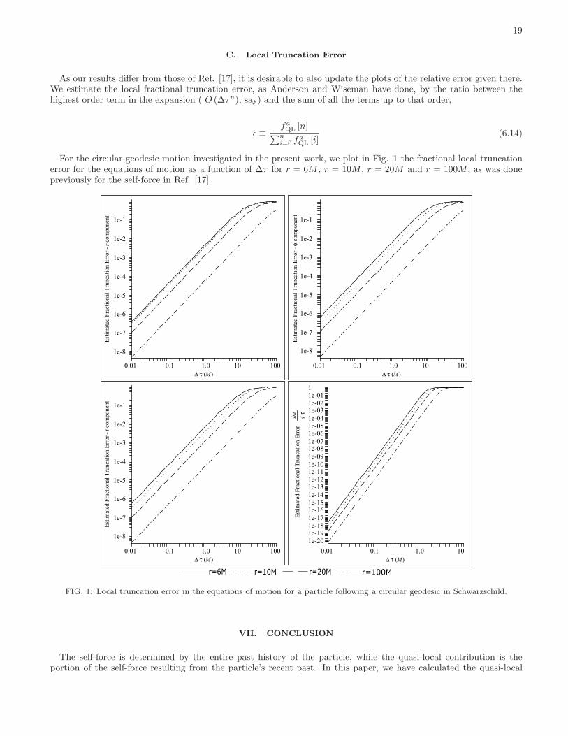
C. Local Truncation Error
As our results differ from those of Ref. [17], it is desirable to also update the plots of the relative error given there.We estimate the local fractional truncation error, as Anderson and Wiseman have done, by the ratio between thehighest order term in the expansion ( O (∆τn), say) and the sum of all the terms up to that order,
ǫ ≡faQL [n]
∑ni=0 fa
QL [i](6.14)
For the circular geodesic motion investigated in the present work, we plot in Fig. 1 the fractional local truncationerror for the equations of motion as a function of ∆τ for r = 6M , r = 10M , r = 20M and r = 100M , as was donepreviously for the self-force in Ref. [17].
D t (M)0.01 0.1 1.0 10 100
Est
imat
ed F
ract
iona
l Tru
ncat
ion
Err
or -
r c
ompo
nent
1e-8
1e-7
1e-6
1e-5
1e-4
1e-3
1e-2
1e-1
D t (M)0.01 0.1 1.0 10 100
Est
imat
ed F
ract
iona
l Tru
ncat
ion
Err
or -
f c
ompo
nent
1e-8
1e-7
1e-6
1e-5
1e-4
1e-3
1e-2
1e-1
D t (M)0.01 0.1 1.0 10 100
Est
imat
ed F
ract
iona
l Tru
ncat
ion
Err
or -
t co
mpo
nent
1e-8
1e-7
1e-6
1e-5
1e-4
1e-3
1e-2
1e-1
D t (M)0.01 0.1 1.0 10
Est
imat
ed F
ract
iona
l Tru
ncat
ion
Err
or -
dm d t
1e-201e-191e-181e-171e-161e-151e-141e-131e-121e-111e-101e-091e-081e-071e-061e-051e-041e-031e-021e-011
FIG. 1: Local truncation error in the equations of motion for a particle following a circular geodesic in Schwarzschild.
VII. CONCLUSION
The self-force is determined by the entire past history of the particle, while the quasi-local contribution is theportion of the self-force resulting from the particle’s recent past. In this paper, we have calculated the quasi-local

20
contribution to the self-force and to the equations of motion for a scalar charge moving in a curved backgroundspacetime. We have determined these quantities up to fifth order in ∆τ , the proper time distance backwards alongthe particle’s path to which the quasi-local contribution applies. In addition to this result, which applies to a generalspacetime, we also present the same result for vacuum spacetimes and show how the expressions simplify significantly.
We then looked at some specific examples of spacetimes and particle motions. We looked at the Schwarzschild andKerr spacetimes and at various geodesic motions. This allowed us to compare our results to existing work and toverify the validity of our approach. It also allowed us to find some errors in some of the existing work.
While Anderson, Eftekharzadeh and Hu have successfully calculated the quasi-local contribution to the self-forceto a much higher order (in ∆τ) than we have done here, their results apply only to a specific choice of spacetimeand to a particular particle motion. On the other hand, the covariant method we describe only provides terms at theleading two orders for massless fields in vacuum spacetimes, but does so for a general vacuum spacetime and general(geodesic) particle motion. In this sense, the two methods are seen as complimentary, each proving as a useful checkon the others results.
We have chosen to restrict the present work to geodesic motion. This was desirable primarily in order to avoidconfusion. Non-geodesic motion adds some extra complexity to the covariant calculation due to there being twodifferent proper times: the particle proper time and the geodesic proper time. We have made significant progress indealing with this issue and intend to present our solution to the problem at a later date.
Obviously, the scalar case as presented here is of less immediate physical interest than the gravitational case. Thebiggest obstacle to achieving results in the gravitational case will be to calculate the relevant DeWitt/Hadamardcoefficients. While this has previously been done for vacuum spacetimes up to O(σ3/2) by Anderson, Flanagan andOttewill [18], it is desirable to take the calculation to higher order to allow the matching point ∆τ to lie furtherinto the particle’s past. It would also be desirable, but not necessary, to obtain expressions for a general spacetime,rather than restricting ourselves to only vacuum spacetimes. Achieving these goals would be possible using a methodsimilar to that of Folacci and Decanini [22], for example. However, it is probable that the expressions would be evenlonger for spin-2 (gravitational) than for spin-0 (scalar) fields. Some hope lies in the fact that we are most interestedcalculating V (x, x′) for massless fields in 4-dimensional vacuum spacetimes. There is also hope that work by Fulling,et al. [33] and more recently by Decanini and Folacci [34] to establish a linearly independent basis for the Riemannpolynomials will simplify the calculation somewhat. Once V (x, x′) has been calculated to sufficiently high order, itwill be straightforward to apply a method analogous the the one presented here to calculate the self-force.
VIII. ACKNOWLEDGMENTS
BW is supported by the Irish Research Council for Science, Engineering and Technology: funded by the NationalDevelopment Plan. We would like to thank Paul Anderson and Ardeshir Eftekharzadeh for the considerable time andeffort they gave to resolving some issues that arose during this work. We would also like to thank Warren Andersonand Antoine Folacci whose ideas and suggestions were invaluable. Also our appreciation to the many others fromthe Capra 10 meeting for interesting and useful conversations. Finally, we would like to thank Marc Casals and SamDolan for their continuous feedback and discussions.
APPENDIX A: CALCULATING COVARIANT HADAMARD/DE-WITT COEFFICIENTS TO 5th ORDERIN THE SEPARATION OF THE POINTS
Folacci and Decanini [22] have calculated the DeWitt and Hadamard coefficients of the Feynman propagator in ageneral spacetime up to O
(
σ2)
in the separation of the points (i.e. fourth order in the geodesic separation of thepoints). In particular, we are interested here in the Hadamard coefficients for the function V (x, x′), which appearsin the Hadamard form of the Feynman propagator.
This may be extended to O(
σ5/2)
relatively easily by taking into account the symmetry V (x, x′) = V (x′, x) ofthe Green’s function. Repeatedly taking symmetrized covariant derivatives of both sides of this equation and takingcoincidence limits, we arrive at an expressions for the odd order terms in terms of all the lower (even) order terms[32]:
n∑
r=0
(
n
r
)
V(a1a2...ar;ar+1...an) = (−1)nVa1a2...an(A1)
Recursively applying this identity to eliminate all odd order terms, we get expressions for the coefficients of the
21
terms of order σ52 :
vabcde =1
2v;(abcde) −
5
2v(ab;cde) +
5
2v(abcd;e) (A2a)
vabc = −1
4v;(abc) +
3
2v(ab;c) (A2b)
va =1
2v;a (A2c)
These expressions are equally valid for any symmetric bi-tensor, so we may use it for both the calculation of higherorder vna1...ap
as used in (3.1) and higher order va1...apas used in (3.7).
APPENDIX B: VACUUM EXPRESSIONS FOR THE HADAMARD/DEWITT COEFFICIENTS
The expressions given in Ref. [22] are unnecessarily long and unwieldy for the purposes of the present work. Weare currently only interested in massless fields in vacuum spacetimes (mfield = 0, Rαβ = 0), so the majority of theterms vanish and we are left with much more manageable expressions for the vna1...ap
. They are:
v0 = 0 (B1a)
v0 a = 0 (B1b)
v0 ab = −1
720gabI (B1c)
v0 abc = −1
480g(abI;c) (B1d)
v0 abcd = −2
525Cρ
(a|σ|b�Cσc|ρ|d) −
2
105Cρστ
(aC|ρστ |b;cd) −1
280C
ρ ;τ(a|σ|b Cσ
c|ρ|d);τ
−1
56Cρστ
(a;bC|ρστ |c;d) −2
1575CρστκCρ(a|τ |bC|σ|c|κ|d) −
2
525Cρκτ
(aCσ
|ρτ | bC|σ|c|κ|d)
−8
1575Cρκτ
(aCσ
|ρ| |τ |bC|σ|c|κ|d) −4
1575Cρτκ
(aCσ
|ρτ | bC|σ|c|κ|d) (B1e)
v1 =1
720I (B1f)
v1 a =1
1440I;a (B1g)
v1 ab = −1
1400CρστκCρστ(a;b)κ +
1
1575Cρστ
a�Cρστb +29
25200CρστκCρστκ;(ab)
+1
1680Cρστ
a;κC ;κρστb +
1
1344Cρστκ
;aCρστκ;b +1
756CρκσλCτ
ρσaCτκλb
−1
1800CρκσλCρστaC τ
κλ b +19
18900CρσκλCρστaC τ
κλ b (B1h)
v2 = −1
6720Cρστκ�Cρστκ −
1
8960Cρστκ;λCρστκ;λ
−1
9072CρκσλCρασβC α β
κ λ −11
18440CρσκλCρσαβC αβ
κλ (B1i)
where Cabcd is the Weyl tensor and I = CαβγδCαβγδ.
Moreover, we have chosen to work with an expression for V (x, x′) as given in (3.7), rather than the expression usedin Ref. [22] and Eq. (3.1). The two sets of coefficients may be related by using
2σ = σ;ασ;α (B2)
to rewrite (3.1) in terms of a series expansion in powers of σ;α. We can then equate, power by power, the coefficients
22
of powers of σ;α to the corresponding terms in (3.7) to give:
v = v0 (B3a)
va = v0 a (B3b)
vab = v0 ab + v1gab (B3c)
vabc = v0 abc + 3v1 (agbc) (B3d)
vabcd = v0 abcd + 6v1 (abgcd) + 6v2g(abgcd) (B3e)
vabcde =1
2v;(abcde) −
5
2v(ab;cde) +
5
2v(abcd;e) (B3f)
Filling in the values for the vn a1...apwe see that a large number of terms either cancel or combine to give:
v = 0 (B4a)
va = 0 (B4b)
vab = 0 (B4c)
vabc = 0 (B4d)
vabcd = −1
280C
ρ σ(a b|;α|C
;α|ρ|c|σ|d) −
2
315CρστκCρ(a|τ |bC|σ|c|κ|d) +
1
105C
ρ σ(a bC
τκ|ρ|cC|τκσ|d)
+1
840CρστκC λ
ρσ (aC|τκλ|bgcd) +1
8960�Ig(abgcd) −
1
40320CρστκC uv
ρσ Cτκuvg(abgcd) (B4e)
vabcde =5
2v(abcd;e) (B4f)
Here, we have used a slight modification of the basis of Riemann tensor polynomials suggested by Fulling, et al.[33] in order to express the result in its simplest possible form. We have chosen an equivalent basis for Weyl tensorpolynomials by ignoring all terms involving Rab and R and replacing Rabcd by Cabcd. We have also ignored allterms which vanish or are not independent under symmetrization of the free indices. Next, we have eliminated termsinvolving two covariant derivatives of a tensor in favor of terms involving two covariant derivatives of a scalar andsingle covariant derivatives of a tensor. We have done this as it is computationally faster and easier to calculate thecovariant derivative of a scalar than of a tensor. Finally, we have used the identity [30]:
∇(r)Cρστ
(a∇(s)C|ρστ |b) =1
4g(ab)∇(r)C
ρστκ∇(s)Cρστκ (B5)
(where ∇(r) indicates r covariant derivatives) to combine some of the remaining terms.The motivation for working with V (x, x′) rather than the Vn(x, x′) is immediately apparent from the vast simplifi-
cation that occurs.
APPENDIX C: CALCULATING COORDINATE HADAMARD/DEWITT COEFFICIENTS TO 7th
ORDER IN THE SEPARATION OF THE POINTS
In order to obtain expressions for the quasi-local equations of motion up to 7th order in the separation of the points,it is first necessary to extend the results of Ref. [31] by one order. As is noted by Ref. [16] and previously by Ref.[32], this is a relatively easy calculation due to the symmetry in the Green’s function:
v (x, x′) = v (x′, x) (C1)
We use expression (6.2) for v (x, x′) in the above to give:
∞∑
i,j,k=0
vijk (r) (t − t′)2i
(cos (γ) − 1)j(r − r′)
k=
∞∑
i,j,k=0
vijk (r′) (t′ − t)2i
(cos (γ′) − 1)j(r′ − r)
k(C2)
Now, in a similar vein to Appendix A, if we take a sufficient number of symmetrized derivatives of both sides andthen take the coincidence limit, it is possible to express odd order coefficients in terms of derivatives of the lower ordercoefficients.
23
For the cases of relevance to the current work, the calculation is made even simpler by spherical symmetry. Thecoefficients vijk are functions of r and M only (i.e. they have no dependence on t or γ). Additionally, since (t − t′)2i
and (cos(γ)− 1)j are both even functions, they are invariant under interchange of primed and unprimed coordinates.This means that we can express (C2) in the simpler form:
∞∑
k=0
vijk (r) (r − r′)k
=
∞∑
k=0
vijk (r′) (r′ − r)k
(C3)
Taking r-derivatives of both sides of this equation and taking the coincidence limit r′ → r gives the result
vij1 = −1
2vij0,r (C4)
For the present work, only the coefficients v301, v211, v121 and v031 are needed. They are given here for convenience:
v301 = −1
960
M2 (r − 2M)2(
598rM2 − 195Mr2 + 20r3 − 585M3)
r16(C5a)
v211 =1
896
M2 (r − 2M)(
3352rM2 − 1099Mr2 + 112r3 − 3240M3)
r13(C5b)
v121 = −9
1120
M2(
228rM2 − 91Mr2 + 12r3 − 189M3)
r10(C5c)
v031 =1
3360
M2(
−155Mr + 56r2 + 36M2)
r7(C5d)
[1] http://www.ligo.caltech.edu/
[2] http://www.virgo.infn.it/
[3] http://geo600.aei.mpg.de/
[4] http://lisa.nasa.gov/
[5] B. S. DeWitt and R. W. Brehme, Annals Phys. 9 (1960) 220.[6] J. M. Hobbs, Annals Phys. 47 (1968) 141.[7] T. C. Quinn and R. M. Wald, Phys. Rev. D 56 (1997) 3381 [arXiv:gr-qc/9610053].[8] Y. Mino, M. Sasaki and T. Tanaka, Phys. Rev. D 55, 3457 (1997) [arXiv:gr-qc/9606018].[9] T. C. Quinn, Phys. Rev. D 62 (2000) 064029 [arXiv:gr-qc/0005030].
[10] S. Detweiler, E. Messaritaki and B. F. Whiting, Phys. Rev. D 67 (2003) 104016 [arXiv:gr-qc/0205079].[11] R. Haas, Phys. Rev. D 75 (2007) 124011 [arXiv:0704.0797 [gr-qc]].[12] L. Barack and N. Sago, Phys. Rev. D 75, 064021 (2007) [arXiv:gr-qc/0701069].[13] L. Barack and D. A. Golbourn, Phys. Rev. D 76, 044020 (2007) [arXiv:0705.3620 [gr-qc]].[14] L. Barack, D. A. Golbourn and N. Sago, arXiv:0709.4588 [gr-qc].[15] A. G. Wiseman, Phys. Rev. D 61 (2000) 084014 [arXiv:gr-qc/0001025].[16] P. R. Anderson, A. Eftekharzadeh and B. L. Hu, Phys. Rev. D 73 (2006) 064023 [arXiv:gr-qc/0507067].[17] W. G. Anderson and A. G. Wiseman, Class. Quant. Grav. 22 (2005) S783 [arXiv:gr-qc/0506136].[18] W. G. Anderson, E. E. Flanagan and A. C. Ottewill, Phys. Rev. D 71 (2005) 024036 [arXiv:gr-qc/0412009].[19] E. Poisson, Living Rev. Rel. 7, 6 (2004) [arXiv:gr-qc/0306052].[20] S. Detweiler, Class. Quant. Grav. 22, S681 (2005) [arXiv:gr-qc/0501004].[21] J. Synge, Relativity: The General Theory (North-Holland, Amsterdam, 1960)[22] Y. Decanini and A. Folacci, Phys. Rev. D 73 (2006) 044027 [arXiv:gr-qc/0511115].[23] C. W. Misner, K. S. Thorne and J. A. Wheeler, Gravitation (Freeman, San Francisco, 1973)[24] M. Casals and A. C. Ottewill, Phys. Rev. D 71, 124016 (2005) [arXiv:gr-qc/0501005].[25] B. S. DeWitt, Dynamical theory of groups and fields (Gordon & Breach, New York, 1965)[26] http://www.grtensor.org/
[27] http://www.maplesoft.com/
[28] S. Chandrasekhar, The Mathematical Theory of Black Holes (Clarendon, Oxford, 1992)[29] J. Hartle, Gravity: An Introduction to Einstein’s General Relativity (Addison-Wesley, San Francisco, 2003)[30] Paul Gunther, Huygens’ Principle and Hyperbolic Equations (Academic Press, London, 1988)[31] P. R. Anderson and B. L. Hu, Phys. Rev. D 69 (2004) 064039 [Erratum-ibid. D 75 (2007) 129901] [arXiv:gr-qc/0308034].
24
[32] M. R. Brown and A. C. Ottewill, Phys. Rev. D 34 (1986) 1776.[33] S. A. Fulling, R. C. King, B. G. Wybourne and C. J. Cummins, Class. Quant. Grav. 9 (1992) 1151.[34] Y. Decanini and A. Folacci (work in preparation), revision to arXiv:gr-qc/0512118.