experimental and modelling study of a geodesic dome solar

EXPERIMENTAL AND MODELLING STUDY OF A

GEODESIC DOME SOLAR GREENHOUSE SYSTEM IN OTTAWA

by

Paula A. Claudino, B.Eng. & Mgmt., Mechanical Engineering and Management

McMaster University, 2006

A thesis submitted to the

Faculty of Graduate and Postdoctoral Affairs

in partial fulfillment of the requirements for the degree of

Master of Applied Science in Sustainable Energy Engineering and Policy

Department of Mechanical and Aerospace Engineering

Carleton University

Ottawa, Ontario

January, 2016

©Copyright

Paula A. Claudino, 2016

ii

Abstract

A building model was created in TRNSYS 17 to determine whether appropriate growing

conditions can be maintained in a geodesic dome greenhouse in Ottawa, Canada, without

the use of auxiliary power or heating. A microcontroller, the Arduino UNO, is used as the

data collection device. In order to test the effects of ventilation, thermal mass, and solar

panel shading on both the modelled and the measured results, combinations of these

variables were used to create five operating scenarios. The model was calibrated and run

under each of these scenarios, using actual 2015 weather data, and was also run for a full

year using the CWEC weather data to compare the performance of each scenario for a

typical weather year. The results indicate that air temperatures are expected to exceed

acceptable ranges during a typical weather year, which indicates that further efforts will

be required to heat and cool the Biodome.

iii

Acknowledgements

This thesis would not have been possible without the help of many dedicated volunteers

from the Brewer Park Community Garden. Thank you to everyone who helped to plan,

build, and maintain the Biodome. I look forward to continuing to work with you on this

project, even after my thesis is complete.

Thank you to my supervisor, Professor Cynthia Cruickshank, for her patience and

support during several false starts, delays, and bursts of work over the course of this

thesis. Her understanding and eternally positive attitude made all the difference in the

world.

Thank you to Professor David Mears in the Department of Plant Biology and

Pathology at Rutgers School of Environmental and Biological Sciences, who provided a

wealth of research materials as well as much appreciated advice on how to heat a

greenhouse in a northern climate.

Finally, thank you to my family for their on-going support, especially my husband,

Stéphane Gagnon, who helped me tremendously, especially when I was trying to learn

how to use the Arduino and set up the data acquisition system. I could not have done this

work without his encouragement.

iv

Table of Contents

Abstract ................................................................................................................................ii

Acknowledgements ............................................................................................................. iii

Table of Contents ................................................................................................................ iv

List of Tables ...................................................................................................................... vii

List of Figures ...................................................................................................................... ix

List of Symbols .................................................................................................................. xiii

List of Abbreviations ......................................................................................................... xiv

List of Appendices .............................................................................................................. xv

1 Introduction ................................................................................................................ 1

1.1 Background ........................................................................................................... 1

1.2 Brewer Park Community Garden Biodome Project ............................................. 5

1.3 Research Objectives ........................................................................................... 19

1.4 Organization of Research and Thesis Document ............................................... 20

2 Literature Review ...................................................................................................... 21

2.1 Introduction........................................................................................................ 21

2.2 Greenhouses ...................................................................................................... 21

2.2.1 Temperature ............................................................................................... 21

2.2.2 Lighting ........................................................................................................ 24

2.2.3 Ventilation and Humidity ............................................................................ 26

2.2.4 Effects of Greenhouse Shape and Orientation on Performance ................ 27

2.3 Geodesic Dome Greenhouses ............................................................................ 28

v

2.4 Thermal Energy Storage ..................................................................................... 31

2.4.1 Water Thermal Energy Storage ................................................................... 33

2.4.2 Rock Bed Thermal Energy Storage .............................................................. 35

2.4.3 Earth-to-Air Heat Exchangers ..................................................................... 36

2.5 Summary ............................................................................................................ 37

3 Modelling and Experimental Approach and Instrumentation .................................. 39

3.1 Introduction........................................................................................................ 39

3.2 Experimental Approach ...................................................................................... 39

3.3 Modelling Approach ........................................................................................... 43

3.3.1 Type 15-5 Weather Data Reading and Processing...................................... 44

3.3.2 Type 56 Multi-Zone Building ....................................................................... 47

3.3.3 Calculators................................................................................................... 55

3.3.4 Printers ........................................................................................................ 56

3.4 Instrumentation and Control System ................................................................. 57

3.4.1 Power .......................................................................................................... 59

3.4.2 Real-Time Clock ........................................................................................... 59

3.4.3 Data Storage Module .................................................................................. 60

3.4.4 Thermocouples ........................................................................................... 61

3.4.5 Humidity Sensors ........................................................................................ 64

3.4.6 Relays .......................................................................................................... 64

3.5 Instrumentation Plan ......................................................................................... 65

3.6 Model Calibration Approach .............................................................................. 67

vi

3.7 Summary ............................................................................................................ 68

4 Results and Discussion .............................................................................................. 69

4.1 Introduction........................................................................................................ 69

4.2 Model Calibration ............................................................................................... 69

4.2.1 Solar Absorptance Calibration .................................................................... 75

4.2.2 Convective Heat Transfer Coefficient Calibration ...................................... 77

4.3 Scenario Results ................................................................................................. 80

4.3.1 Scenario A ................................................................................................... 81

4.3.2 Scenario B ................................................................................................... 84

4.3.3 Scenario C.................................................................................................... 87

4.3.4 Scenario D ................................................................................................... 90

4.3.5 Scenario E .................................................................................................... 93

4.4 Scenario Comparison ......................................................................................... 96

4.5 Uncertainty Analysis ........................................................................................... 97

4.6 Summary .......................................................................................................... 101

5 Contributions .......................................................................................................... 103

6 Conclusions and Future Work ................................................................................. 106

References ...................................................................................................................... 109

vii

List of Tables

Table 1: Suggested radiant energy, duration, and time of day for supplemental lighting in

greenhouses (adapted from 2011 ASHRAE Handbook, Table 10). ................................... 25

Table 2: Heat capacity of materials used for heat storage (Adapted from Table 4 of Energy-

Conserving Urban Greenhouses for Canada, Agriculture Canada, 1987). ....................... 32

Table 3: Empirical relationships between water storage volumes used for given

greenhouse ground areas using different cover materials and storage material (Adapted

from Table 2 in Sethi and Sharma, 2008). ........................................................................ 34

Table 4: Empirical relationships between heat capacity of rock bed storage and


from Table 4 in Sethi and Sharma, 2008). ........................................................................ 36

Table 5: Summary of the performance of various agricultural greenhouses using an earth-

to-air heat exchanger system (Adapted from: Table 7 from Sethi and Sharma, 2008). .. 38

Table 6: Biodome operating scenarios ............................................................................. 39

Table 7: Evaluation of three possible solar panel mounting configurations. ................... 42

Table 8: Initial properties of modelled Biodome zones. ................................................... 49

Table 9: Layers used in the TRNSYS model. ...................................................................... 52

Table 10: Layer composition of each component used in the TRNSYS model. ................ 52

Table 11: Properties of each component used in the Biodome TRNSYS model. ............. 53

Table 12: Estimated infiltration rates for greenhouses by type and construction (Adapted

from ASABE, 2008). ........................................................................................................... 54

Table 13: Thermocouple locations. .................................................................................. 66

viii

Table 14: Correlation between measured and modelled air and soil temperature. ....... 72

Table 15: Effect on modelled results of changing soil surface solar absorptance. .......... 76

Table 16: Effect on modelled results of changing soil surface convective heat transfer

coefficient. ........................................................................................................................ 78

Table 17: Linear trend line equations of measured versus modelled air and soil

temperatures for different convective heat transfer coefficients of the soil surface. ..... 80

Table 18: Hours per year above maximum temperature thresholds, by scenario .......... 96

Table 19: hours per year below minimum temperature thresholds, by scenario ........... 97

Table 20: Thermal characteristics of the MAX31850K (Adapted from: Maxim, 2013). ... 99

ix

List of Figures

Figure 1: Area of fruit and vegetable greenhouses in Canada, by Province from 2010 to

2015. (Statistics Canada. CANSIM Table 001-0047) ........................................................... 3

Figure 2: Map of location of BPCG in Ottawa (Google maps, 2015) .................................. 6

Figure 3: Aerial view of Biodome (Google maps, 2015b) ................................................... 6

Figure 4: Three different geodesic dome shapes that were considered. ........................... 9

Figure 5: Architectural drawing of proposed Biodome layout (Christopher Simmonds

Architect Inc., 2014). Adapted with permission. .............................................................. 10

Figure 6: Architectural drawing of Biodome location (Christopher Simmonds Architect

Inc., 2014). Adapted with permission. .............................................................................. 11

Figure 7: Architectural drawing of Biodome structure and wall detail (Christopher

Simmonds Architect Inc., 2014). Adapted with permission. ............................................ 12

Figure 8: Layout of insulation before installation (E. Kucerak, personal photograph, April

26, 2014). Adapted with permission. ................................................................................ 12

Figure 9: Installation of EPS insulation on site (E. Kucerak, personal photograph, May 2,

2014). Adapted with permission....................................................................................... 13

Figure 10: Layout of earth to air heat exchanger piping (E. Kucerak, personal photograph,

May 3, 2014). Adapted with permission. .......................................................................... 14

Figure 11: Installation of earth to air heat exchanger piping (E. Kucerak, personal

photograph, May 3, 2014). Adapted with permission...................................................... 14

Figure 12: Top view of placement of underground pipes in the Biodome. ...................... 15

Figure 13: Cross-sectional view of placement of underground pipes. ............................. 16

x

Figure 14: Earth-to-air heat exchanger air intake box (left), air outlet box 1 (middle), and

air outlet box 1 vent (right). .............................................................................................. 16

Figure 15: Installation of base plates (E. Kucerak, personal photograph, May 25, 2014).

Adapted with permission. ................................................................................................. 17

Figure 16: Installation of base walls (left) (E. Kucerak, personal photograph, May 26, 2014)

and trusses (right) (E. Kucerak, personal photograph, May 29, 2014). Adapted with

permission. ........................................................................................................................ 17

Figure 17: Completed Biodome structure (E. Kucerak, personal photograph, September

19, 2014). Adapted with permission. ................................................................................ 18

Figure 18: Energy flow pathways in a greenhouse. .......................................................... 23

Figure 19: Icosahedron centred at the origin. .................................................................. 29

Figure 20: Relationship between icosahedron equilateral triangle face subdivisions and

geodesic dome frequency. ................................................................................................ 29

Figure 21: Intermediate bulk container to be used as a water storage tank (E. Kucerak,

personal photograph, October 25, 2014). Adapted with permission. ............................. 40

Figure 22: Three possible solar panel mounting configurations, 1, 2, and 3, from left to

right. .................................................................................................................................. 41

Figure 23: Installed solar panels (E. Kucerak, personal photograph, June 25, 2015).

Adapted with permission. ................................................................................................. 42

Figure 24: Biodome TRNSYS model. ................................................................................. 44

Figure 25: Top-view and identification of planter bed zones, air spaces, and water storage

tank area. .......................................................................................................................... 48

xi

Figure 26: 3D Model of Biodome in SketchUp. ................................................................ 49

Figure 27: Representative window detail. ........................................................................ 51

Figure 28: Schematic of Arduino UNO pin assignments. .................................................. 58

Figure 29: Real-time clock module pin diagram. .............................................................. 60

Figure 30: MicroSD card breakout board pin diagram. .................................................... 60

Figure 31: Thermocouple amplifier breakout board pin diagram. ................................... 62

Figure 32: Logic level converter and pin diagram. ............................................................ 62

Figure 33: Assembled thermocouple breakout boards connected in series. ................... 63

Figure 34: DHT22 Temperature and humidity sensor pin diagram. ................................. 64

Figure 35: Relay module pin diagram. .............................................................................. 65

Figure 36: Measured Biodome and outdoor air temperatures for hours 1944 to 2304. . 70

Figure 37: Measured Biodome underground air and soil temperatures for hours 1944 to

2304. ................................................................................................................................. 72

Figure 38: Time series plot of Model 1 and measured air and soil temperatures in the

Biodome over the calibration period. ............................................................................... 74

Figure 39: Scatter plot of Model 1 results versus measured Biodome air and soil

temperatures over the calibration period. ....................................................................... 74

Figure 40: Graph of effect on modelled results of changing soil surface solar absorptance.

........................................................................................................................................... 76

Figure 41: Scatter plot of effect on modelled results of changing soil surface solar

absorptance. ..................................................................................................................... 77

Figure 42: Graph of effect on modelled results of changes in modelled convective heat

xii

transfer coefficient of the soil surface. ............................................................................. 79

Figure 43: Time series plot of Scenario A modelled and measured air and soil

temperatures in the Biodome. ......................................................................................... 82

Figure 44: Scatter plot of Scenario A results versus measured Biodome air and soil

temperatures for the same period. .................................................................................. 83

Figure 45: Time series plot of Scenario B modelled and measured air and soil


Figure 46: Scatter plot of Scenario B results versus measured Biodome air and soil


Figure 47: Time series plot of Scenario C modelled and measured air and soil temperatures

in the Biodome. ................................................................................................................. 88

Figure 48: Scatter plot of Scenario C results versus measured Biodome air and soil


Figure 49: Time series plot of Scenario D modelled and measured air and soil


Figure 50: Scatter plot of Scenario D results versus measured Biodome air and soil


Figure 51: Time series plot of Scenario E modelled and measured air and soil temperatures

in the Biodome. ................................................................................................................. 94

Figure 52: Scatter plot of Scenario E results versus measured Biodome air and soil


xiii

List of Symbols

A surface area, m2

N number of air changes per hour, h-1

qc conduction, W

qi infiltration, W

qt total peak heating requirements, W

r sample correlation coefficient

r2 Pearson coefficient of determination

TA temperature of the device, or the cold-junction, oC

ti inside temperature, oC

to outside temperature, oC

TR temperature of the remote thermocouple junction, or hot-junction, oC

U overall heat loss coefficient, W/(m2 K)

V greenhouse internal volume, m3

v geodesic dome frequency

VOUT thermocouple output voltage, µV

X greenhouse floor area, m2

x� deviation of observed data from the sample means

x� deviation of the simulated data from the sample means

Yr heat capacity of rock storage, kJ/oC

Yw volume of water storage, kL

xiv

List of Abbreviations

ASABE American Society of Agricultural and Biological Engineers

BPCG Brewer Park Community Garden

IC Integrated circuit

CO2 Carbon dioxide

CWEC Canadian weather for energy calculations

EAHE Earth-to-air heat exchanger

EPS Expanded polystyrene

PCSS Polycarbonate structured sheet

xv

List of Appendices

Appendix A: Arduino Program

Appendix B: TRNSYS Input File

Appendix C: TRNSYS Deck File

1

Chapter 1

1

Introduction

1.1 Background

There is increased interest in locally-grown food in Canada, and specifically in Ontario, as

evidenced by the passage of the Ontario Local Food Act (Bill C-36, 2013). The purpose of

this legislation, the first of its kind in Canada, is to promote local food awareness and

increase sales of Ontario produce by setting local food goals and targets. An Ipsos-Reid

survey (2006) found that Canadians believe the benefits of buying locally-grown produce

include:

• Help their local economy (71%)

• Support family farmers (70%)

• Taste better (53%)

• Are Cheaper (50%)

• Not genetically modified (48%)

• Healthier (46%)

• No chemical / Synthetic pesticides (45%)

• Safer (44%)

• Environmentally friendly (43%)

The increased interest in locally grown food is also evident from the growing

number of community gardens, which are enjoying increased popularity in many

Canadian urban centres, such as Montreal, Ottawa, Toronto, and Vancouver.

In 2006, Vancouver City Council issued a community challenge to “create 2010

2

new garden plots by 2010, as an Olympic legacy" (Reichel, 2012). This challenge was

exceeded by the beginning of 2010 (Reichel, 2012) and was replaced by the mayor's goal

to reach 5000 garden plots in the City of Vancouver by 2020, as part of Vancouver's

Greenest City Action Plan (Vancouver, 2012).

This increased interest in community gardening is also being seen in Ottawa,

Ontario, where, according to the Ottawa Deputy City Manager's report (Ottawa, 2009),

"each year, interest in and demand for community gardens increase, influenced by rising

food costs and gas prices, concerns about food security, interest in growing and eating

locally-produced food, urban greening projects and urban agriculture." As of July 2015,

the city of Ottawa had 48 community gardens, including one city-run allotment garden

(Just Food, 2015), an increase of 153 percent from 2008, when there were 19 community

gardens in Ottawa (Ottawa, 2009).

In more temperate climates, such as that of Vancouver, some community gardens

are maintained year-round (Reichel, 2012) but in Ottawa, community gardens are

typically open for only six months a year, from mid-May to mid-October, as the

temperature is prohibitively low for gardening during the remainder of the year. In order

to extend the growing season, some community garden organizations have started to

construct community greenhouse gardens.

For example, the Banff Greenhouse Gardening Society (BGGS) operates two

community greenhouses in Banff, Alberta. The first greenhouse, built in 2011, is 6.1 m by

14.6 m and houses 34 individual 1.5 m2 plots. The second greenhouse, built in 2013, is

6.1 m by 9.1 m and houses 20 individual 1.4 m2 plots (BGGS, 2013).

3

Greenhouses allow farmers and gardeners to extend the growing season by

providing a controlled growing space, leading to increased yields due to the longer

growing season, optimized growing conditions, and the ability to grow plants that would

otherwise not survive in a given climate. One of the trade-offs, however, is that

greenhouses can be more energy intensive than other forms of agriculture, especially if

energy is required to ventilate or heat the space and if supplemental lighting is provided.

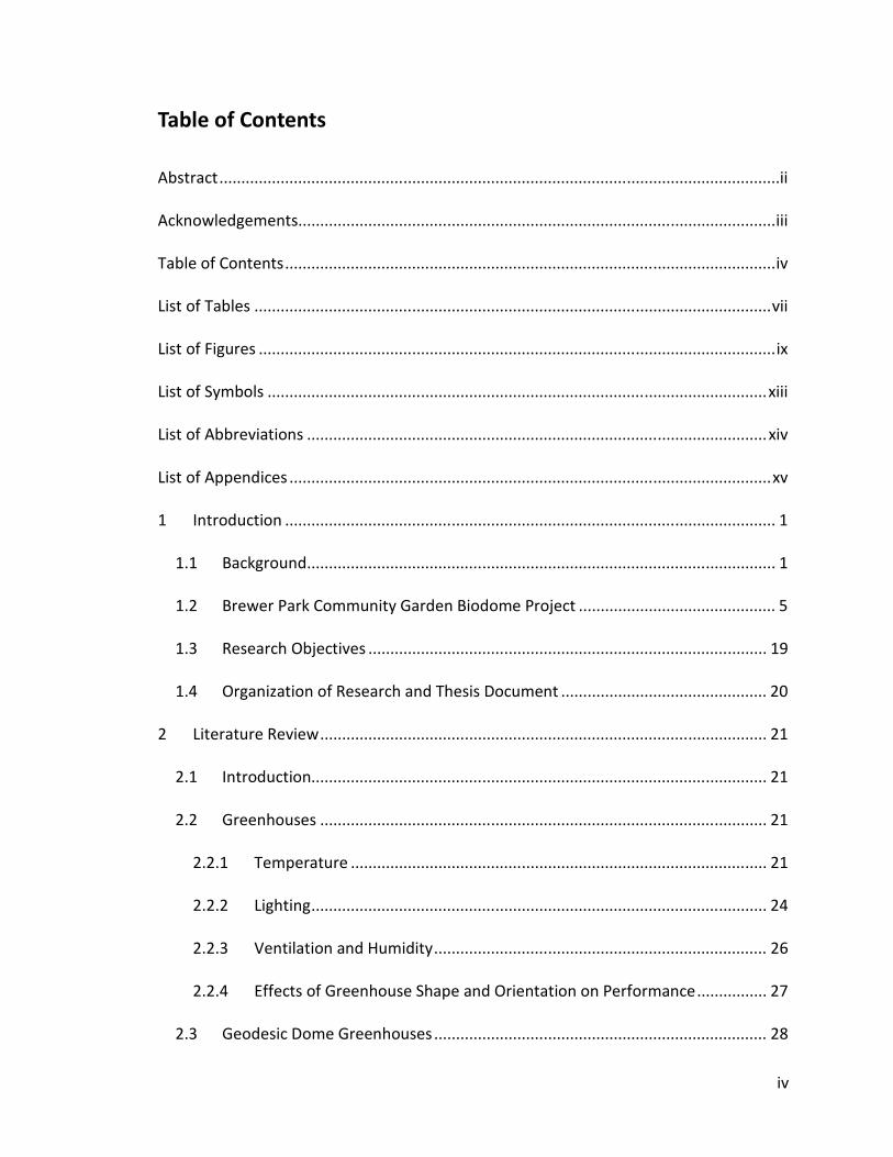
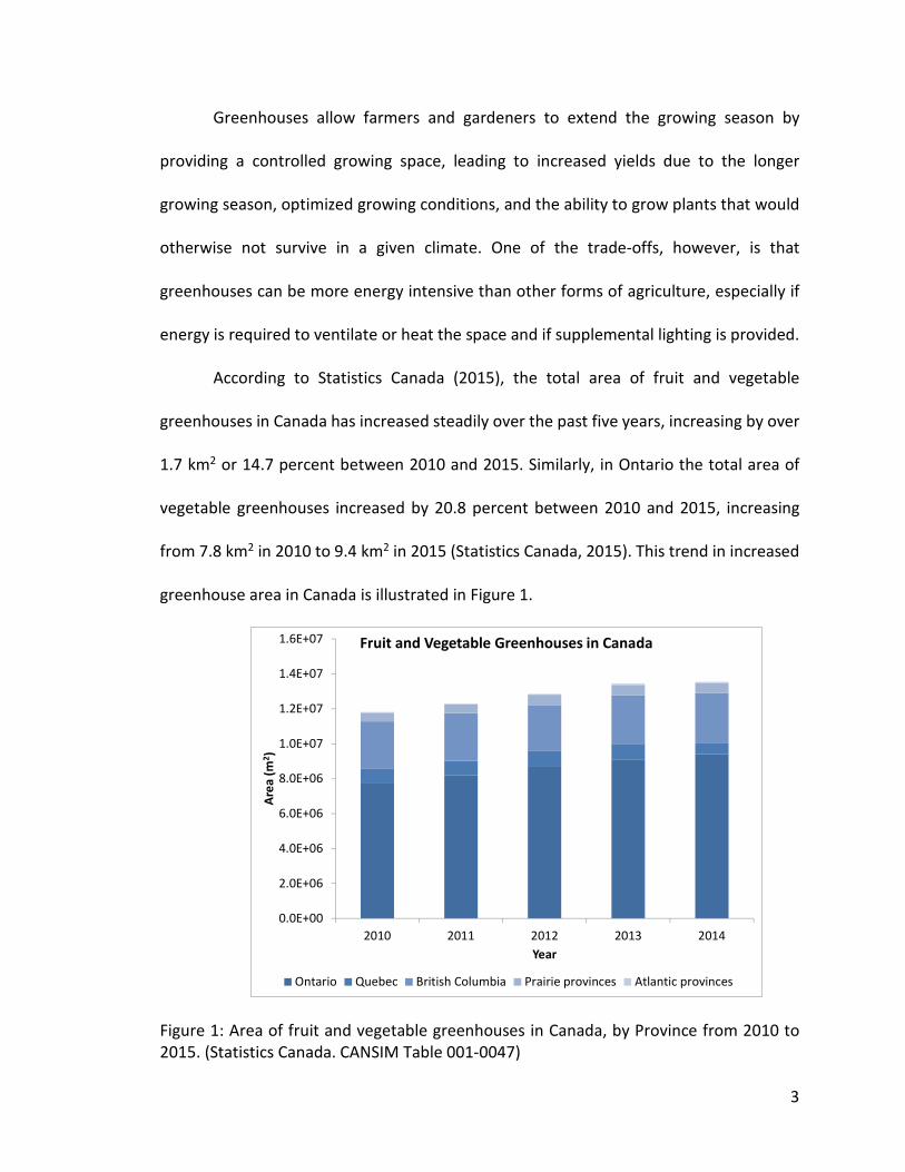
According to Statistics Canada (2015), the total area of fruit and vegetable

greenhouses in Canada has increased steadily over the past five years, increasing by over

1.7 km2 or 14.7 percent between 2010 and 2015. Similarly, in Ontario the total area of

vegetable greenhouses increased by 20.8 percent between 2010 and 2015, increasing

from 7.8 km2 in 2010 to 9.4 km2 in 2015 (Statistics Canada, 2015). This trend in increased

greenhouse area in Canada is illustrated in Figure 1.

Figure 1: Area of fruit and vegetable greenhouses in Canada, by Province from 2010 to

2015. (Statistics Canada. CANSIM Table 001-0047)

0.0E+00

2.0E+06

4.0E+06

6.0E+06

8.0E+06

1.0E+07

1.2E+07

1.4E+07

1.6E+07

2010 2011 2012 2013 2014

Are

a (

m2)

Year

Fruit and Vegetable Greenhouses in Canada

Ontario Quebec British Columbia Prairie provinces Atlantic provinces

4

Greenhouses are also being considered in more and more extreme environments,

such as in Canada’s far north. In August 2014, Prime Minister Stephen Harper announced

measures to promote northern agriculture, including the launch of the Northern

Greenhouse Initiative, aimed at “advancing the commercialization and enhancing the

productivity of greenhouse projects across Canada’s North” (Prime Minister of Canada

Stephen Harper, 2014). The construction of commercial or community greenhouses in the

north would contribute to improved health of the local population due to the increased

availability of better quality food, increased food security, and to science education and

skills training (Exner-Pirot, 2012).

One of the challenges for community greenhouses, especially in cold climates, is

the availability of and access to supplementary energy that is typically necessary to

maintain year-round operation. A greenhouse design that is able to minimize or eliminate

the need for supplementary energy would greatly contribute to the potential for the

successful implantation of greenhouse operations in northern community gardens.

In addition to providing the conditions necessary to grow plants, greenhouses can

also be used to grow animal protein, in the form of fish. The combination of hydroponics

(the cultivation of plants in nutrient-rich water instead of soil) and aquaculture (raising

aquatic animals in tanks) has been termed Aquaponics (Diver, 2006). Some of the benefits

of including an Aquaponics system in a greenhouse are that the water tanks act as thermal

energy storage for the greenhouse and the fish can provide more CO2 for the plants. The

greenhouse also acts as a passive solar collector, reducing the amount of additional

energy needed for heat.

5

1.2 Brewer Park Community Garden Biodome Project

Brewer Park Community Garden (BPCG) is a registered non-profit organization that

operates a community garden located in Brewer Park, in the area of Old Ottawa South, in

Ottawa, Ontario. Membership in BPCG is open to people who live, work, or study in Old

Ottawa South and neighbouring areas. The garden is currently composed of some 50

raised garden beds that are used by members to grow food.

One of the goals of the BPCG is to contribute to local food security and community

development (BPCG, 2013). As such, one of the key projects undertaken by BPGC

beginning in 2013 was the design, construction, and operation of a geodesic dome-

shaped community garden greenhouse, referred to hereafter as the Biodome. The

purpose of the Biodome is to showcase different growing methods and support member-

driven educational projects that benefit the Garden's members and the local community.

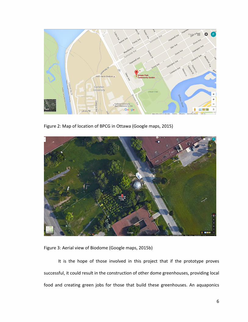
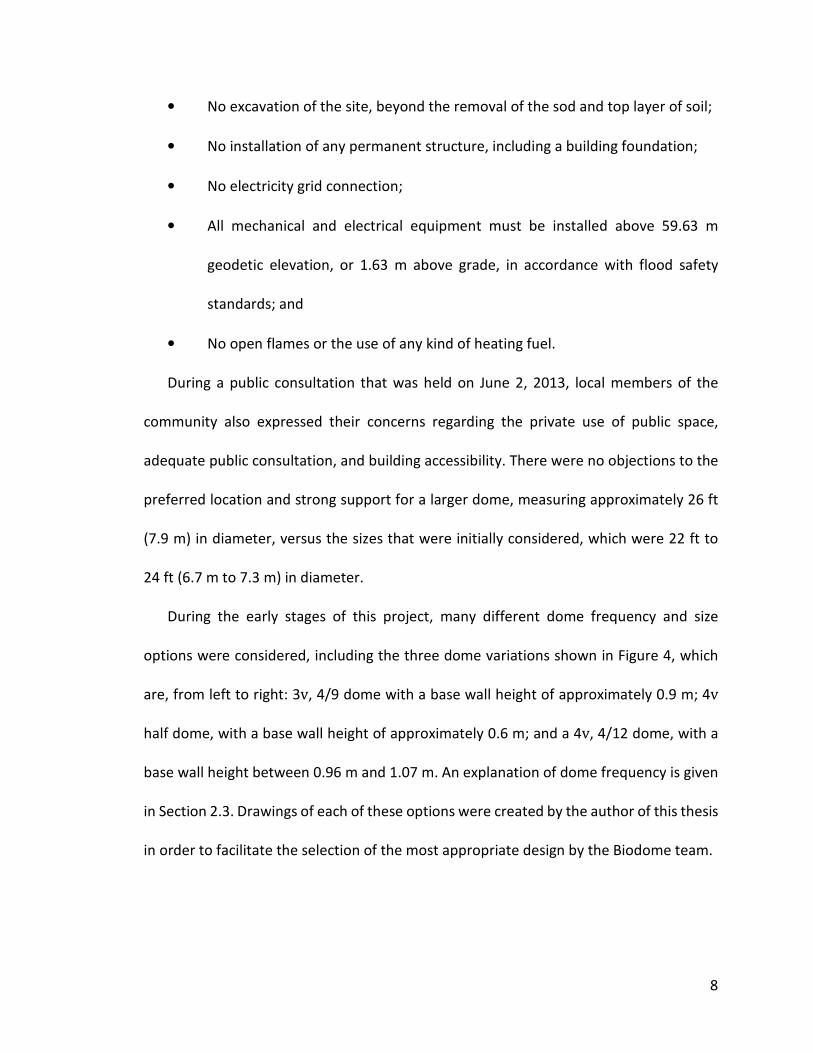
The Biodome is located on the same site as the community garden, as shown in Figure 2

and Figure 3.

The Biodome is located in Brewer Park, a municipal park in Ottawa, Ontario,

Canada, across from Carleton University. Located at 45oN, 75oW, Ottawa has a humid

continental, or Dfb classification, climate according to the widely used Köppen-Geiger

climate classification system (Rubel, 2010). The temperature in Ottawa can range from an

extreme minimum of -38.9oC in winter to an extreme maximum of 37.8oC in summer

(Environment Canada, 2015). These wide temperature swings make it exceptionally

challenging to maintain a consistent internal operating temperature, with both heating

and cooling being required throughout the year.

6

Figure 2: Map of location of BPCG in Ottawa (Google maps, 2015)

Figure 3: Aerial view of Biodome (Google maps, 2015b)

It is the hope of those involved in this project that if the prototype proves

successful, it could result in the construction of other dome greenhouses, providing local

food and creating green jobs for those that build these greenhouses. An aquaponics

7

system is planned for the Biodome, but this study will not focus on the design or operation

of the aquaponics system, other than the temperature of the tanks and their use as

thermal energy storage.

Planning for this project began in 2011 and the goal was to build the Biodome in

2013, but construction was delayed by planning and permitting issues. The author of this

thesis joined the Biodome team in March 2013, in the role of Energy Lead, and provided

guidance and support during the design, public consultation, construction, and

implementation phases of this project. Construction began in April 2014 and the

Biodome’s grand-opening was held on August 17, 2014.

The Biodome received funding from the following organizations:

• The City of Ottawa Better Neighbourhoods Program;

• TD Friends of the Environment Foundation; and

• Just Food and the Community Garden Network.

The Biodome was built by Future Food Bio-dome Systems; the Ottawa architecture

firm, Christopher Simmonds Architect Inc., created architectural drawings for the building

and provided guidance in applying for building permits; structural engineering services

were provided by Cleland Jardine Engineering Ltd.; and geotechnical engineering services,

including soil bearing and frost protection analysis, were provided by Peterson Group

Consulting Engineers. Project management and on-going operations are provided by a

group of volunteers composed of local community members.

As the Biodome is located in a municipal public park and is in a floodplain, there were

certain restrictions to the design of the structure, including the following:

8

• No excavation of the site, beyond the removal of the sod and top layer of soil;

• No installation of any permanent structure, including a building foundation;

• No electricity grid connection;

• All mechanical and electrical equipment must be installed above 59.63 m

geodetic elevation, or 1.63 m above grade, in accordance with flood safety

standards; and

• No open flames or the use of any kind of heating fuel.

During a public consultation that was held on June 2, 2013, local members of the

community also expressed their concerns regarding the private use of public space,

adequate public consultation, and building accessibility. There were no objections to the

preferred location and strong support for a larger dome, measuring approximately 26 ft

(7.9 m) in diameter, versus the sizes that were initially considered, which were 22 ft to

24 ft (6.7 m to 7.3 m) in diameter.

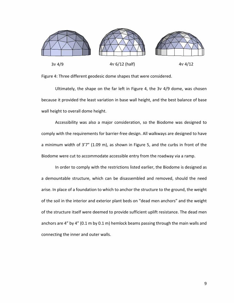
During the early stages of this project, many different dome frequency and size

options were considered, including the three dome variations shown in Figure 4, which

are, from left to right: 3v, 4/9 dome with a base wall height of approximately 0.9 m; 4v

half dome, with a base wall height of approximately 0.6 m; and a 4v, 4/12 dome, with a

base wall height between 0.96 m and 1.07 m. An explanation of dome frequency is given

in Section 2.3. Drawings of each of these options were created by the author of this thesis

in order to facilitate the selection of the most appropriate design by the Biodome team.

9

Figure 4: Three different geodesic dome shapes that were considered.

Ultimately, the shape on the far left in Figure 4, the 3v 4/9 dome, was chosen

because it provided the least variation in base wall height, and the best balance of base

wall height to overall dome height.

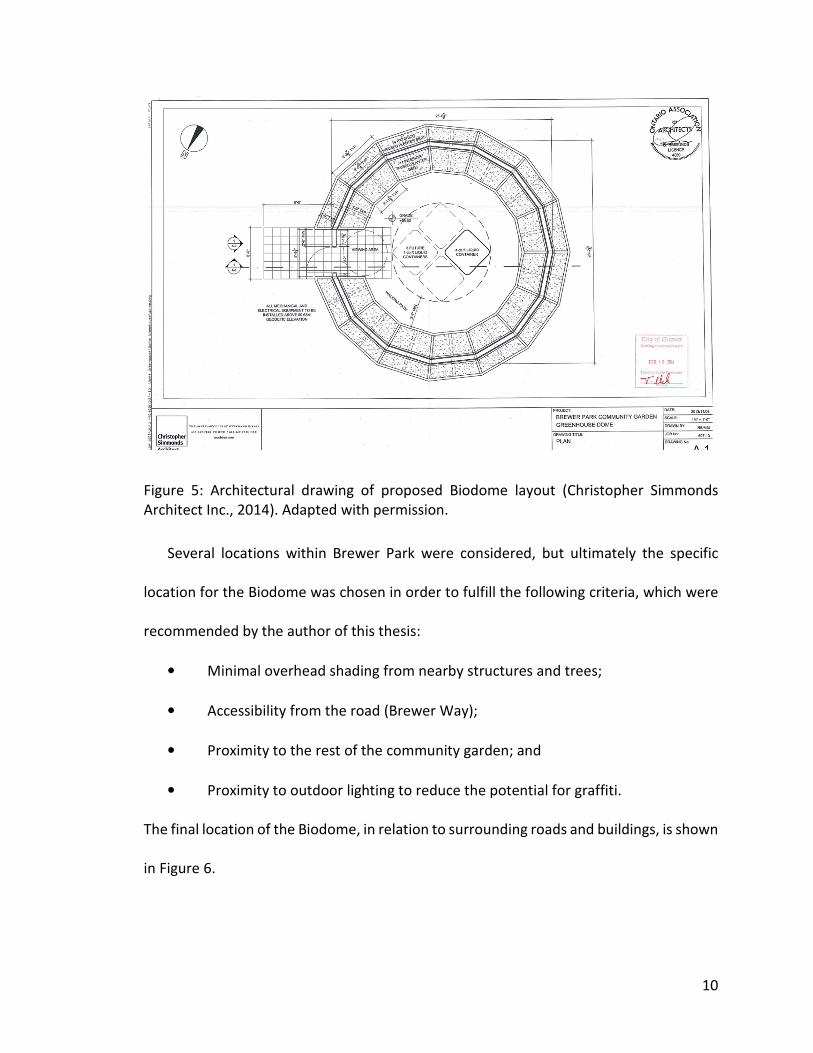
Accessibility was also a major consideration, so the Biodome was designed to

comply with the requirements for barrier-free design. All walkways are designed to have

a minimum width of 3’7” (1.09 m), as shown in Figure 5, and the curbs in front of the

Biodome were cut to accommodate accessible entry from the roadway via a ramp.

In order to comply with the restrictions listed earlier, the Biodome is designed as

a demountable structure, which can be disassembled and removed, should the need

arise. In place of a foundation to which to anchor the structure to the ground, the weight

of the soil in the interior and exterior plant beds on “dead men anchors” and the weight

of the structure itself were deemed to provide sufficient uplift resistance. The dead men

anchors are 4” by 4” (0.1 m by 0.1 m) hemlock beams passing through the main walls and

connecting the inner and outer walls.

3v 4/9 4v 6/12 (half) 4v 4/12

10

Figure 5: Architectural drawing of proposed Biodome layout (Christopher Simmonds

Architect Inc., 2014). Adapted with permission.

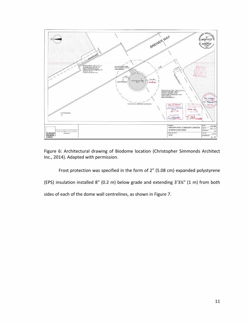
Several locations within Brewer Park were considered, but ultimately the specific

location for the Biodome was chosen in order to fulfill the following criteria, which were

recommended by the author of this thesis:

• Minimal overhead shading from nearby structures and trees;

• Accessibility from the road (Brewer Way);

• Proximity to the rest of the community garden; and

• Proximity to outdoor lighting to reduce the potential for graffiti.

The final location of the Biodome, in relation to surrounding roads and buildings, is shown

in Figure 6.

11

Figure 6: Architectural drawing of Biodome location (Christopher Simmonds Architect

Inc., 2014). Adapted with permission.

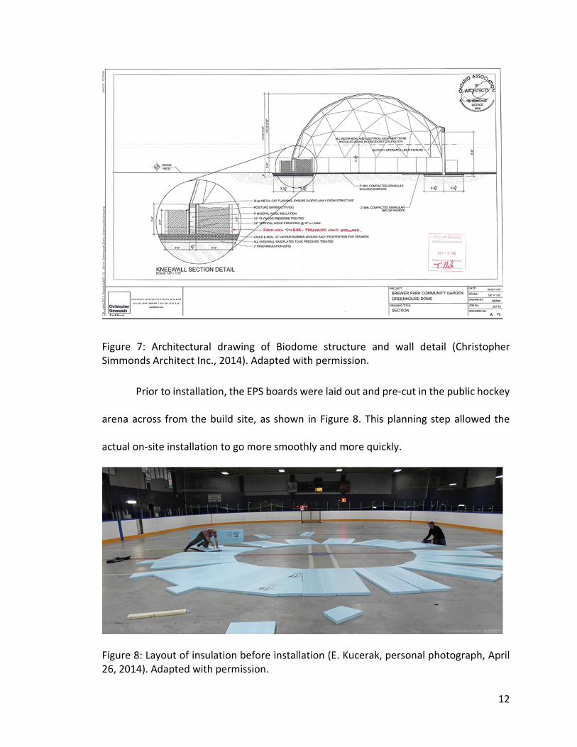
Frost protection was specified in the form of 2” (5.08 cm) expanded polystyrene

(EPS) insulation installed 8” (0.2 m) below grade and extending 3’3¼” (1 m) from both

sides of each of the dome wall centrelines, as shown in Figure 7.

12

Figure 7: Architectural drawing of Biodome structure and wall detail (Christopher

Simmonds Architect Inc., 2014). Adapted with permission.

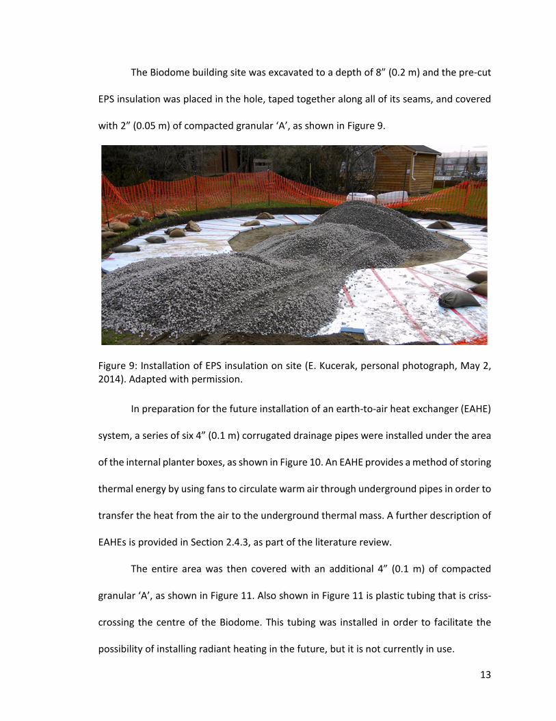
Prior to installation, the EPS boards were laid out and pre-cut in the public hockey

arena across from the build site, as shown in Figure 8. This planning step allowed the

actual on-site installation to go more smoothly and more quickly.

Figure 8: Layout of insulation before installation (E. Kucerak, personal photograph, April

26, 2014). Adapted with permission.

13

The Biodome building site was excavated to a depth of 8” (0.2 m) and the pre-cut

EPS insulation was placed in the hole, taped together along all of its seams, and covered

with 2” (0.05 m) of compacted granular ‘A’, as shown in Figure 9.

Figure 9: Installation of EPS insulation on site (E. Kucerak, personal photograph, May 2,

2014). Adapted with permission.

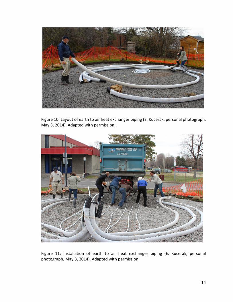
In preparation for the future installation of an earth-to-air heat exchanger (EAHE)

system, a series of six 4” (0.1 m) corrugated drainage pipes were installed under the area

of the internal planter boxes, as shown in Figure 10. An EAHE provides a method of storing

thermal energy by using fans to circulate warm air through underground pipes in order to

transfer the heat from the air to the underground thermal mass. A further description of

EAHEs is provided in Section 2.4.3, as part of the literature review.

The entire area was then covered with an additional 4” (0.1 m) of compacted

granular ‘A’, as shown in Figure 11. Also shown in Figure 11 is plastic tubing that is criss-

crossing the centre of the Biodome. This tubing was installed in order to facilitate the

possibility of installing radiant heating in the future, but it is not currently in use.

14

Figure 10: Layout of earth to air heat exchanger piping (E. Kucerak, personal photograph,

May 3, 2014). Adapted with permission.

Figure 11: Installation of earth to air heat exchanger piping (E. Kucerak, personal

photograph, May 3, 2014). Adapted with permission.

15

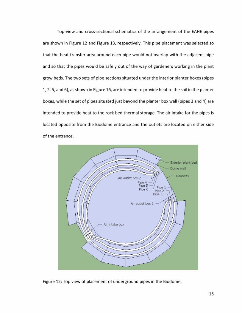
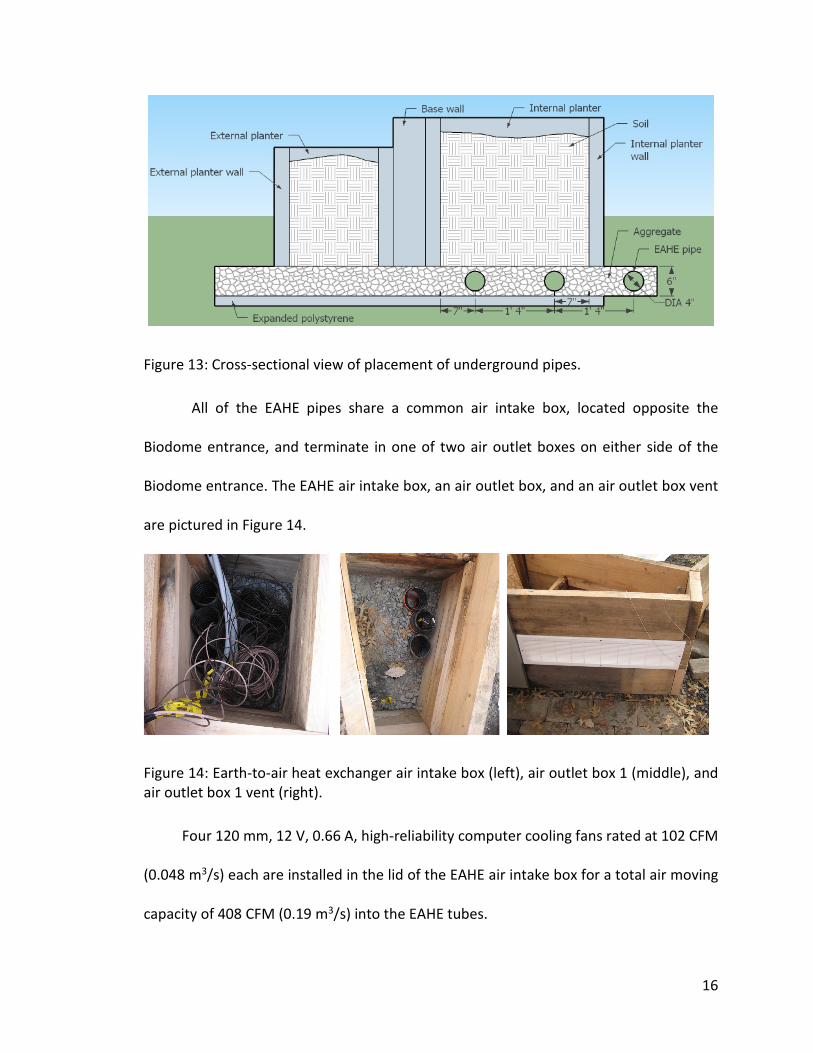
Top-view and cross-sectional schematics of the arrangement of the EAHE pipes

are shown in Figure 12 and Figure 13, respectively. This pipe placement was selected so

that the heat transfer area around each pipe would not overlap with the adjacent pipe

and so that the pipes would be safely out of the way of gardeners working in the plant

grow beds. The two sets of pipe sections situated under the interior planter boxes (pipes

1, 2, 5, and 6), as shown in Figure 16, are intended to provide heat to the soil in the planter

boxes, while the set of pipes situated just beyond the planter box wall (pipes 3 and 4) are

intended to provide heat to the rock bed thermal storage. The air intake for the pipes is

located opposite from the Biodome entrance and the outlets are located on either side

of the entrance.

Figure 12: Top view of placement of underground pipes in the Biodome.

16

Figure 13: Cross-sectional view of placement of underground pipes.

All of the EAHE pipes share a common air intake box, located opposite the

Biodome entrance, and terminate in one of two air outlet boxes on either side of the

Biodome entrance. The EAHE air intake box, an air outlet box, and an air outlet box vent

are pictured in Figure 14.

Figure 14: Earth-to-air heat exchanger air intake box (left), air outlet box 1 (middle), and

air outlet box 1 vent (right).

Four 120 mm, 12 V, 0.66 A, high-reliability computer cooling fans rated at 102 CFM

(0.048 m3/s) each are installed in the lid of the EAHE air intake box for a total air moving

capacity of 408 CFM (0.19 m3/s) into the EAHE tubes.

17

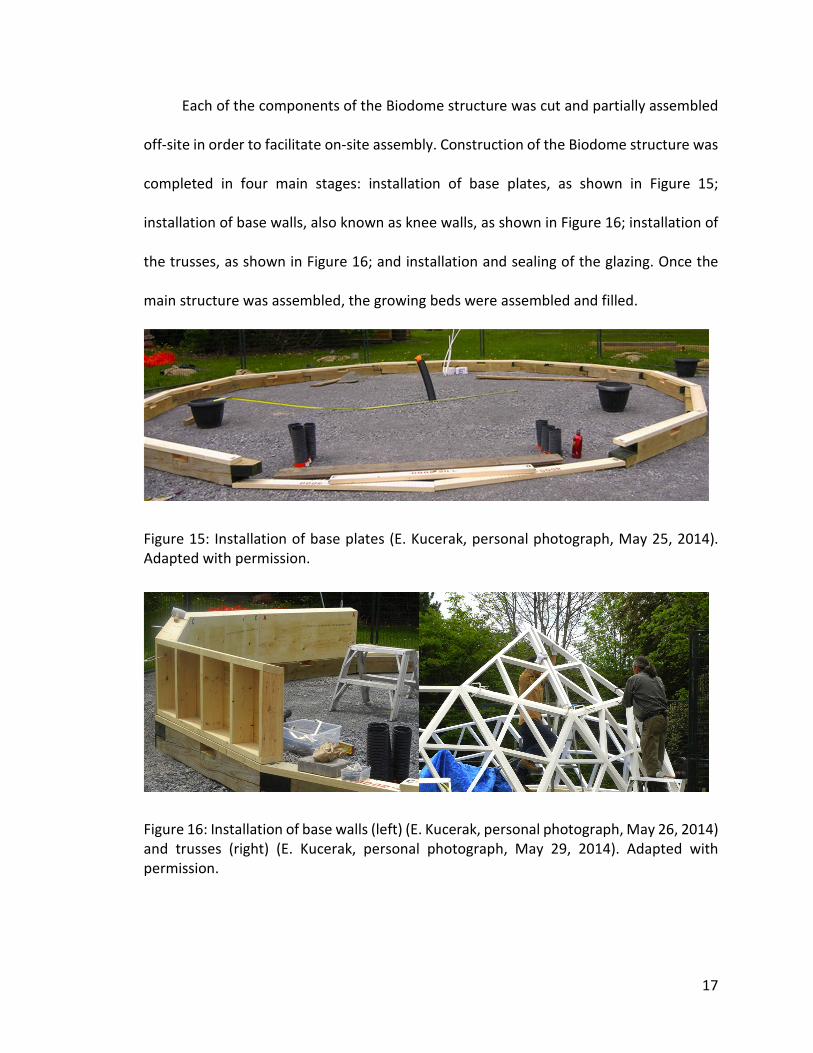
Each of the components of the Biodome structure was cut and partially assembled

off-site in order to facilitate on-site assembly. Construction of the Biodome structure was

completed in four main stages: installation of base plates, as shown in Figure 15;

installation of base walls, also known as knee walls, as shown in Figure 16; installation of

the trusses, as shown in Figure 16; and installation and sealing of the glazing. Once the

main structure was assembled, the growing beds were assembled and filled.

Figure 15: Installation of base plates (E. Kucerak, personal photograph, May 25, 2014).

Adapted with permission.

Figure 16: Installation of base walls (left) (E. Kucerak, personal photograph, May 26, 2014)

and trusses (right) (E. Kucerak, personal photograph, May 29, 2014). Adapted with

permission.

18

The dome glazing material is a triple-wall co-extruded polycarbonate with UV

protection on the inner surface to reduce solar degradation of the polycarbonate. This

material provides good performance, in terms of light transmission and insulation, and is

significantly lighter than glass (Moretti, Zinzi, and Belloni, 2013). Polycarbonate has the

added advantage that, unlike glass, it is virtually shatterproof; with an impact resistance

of over 200 times that of tempered glass, which is an added benefit in a public space.

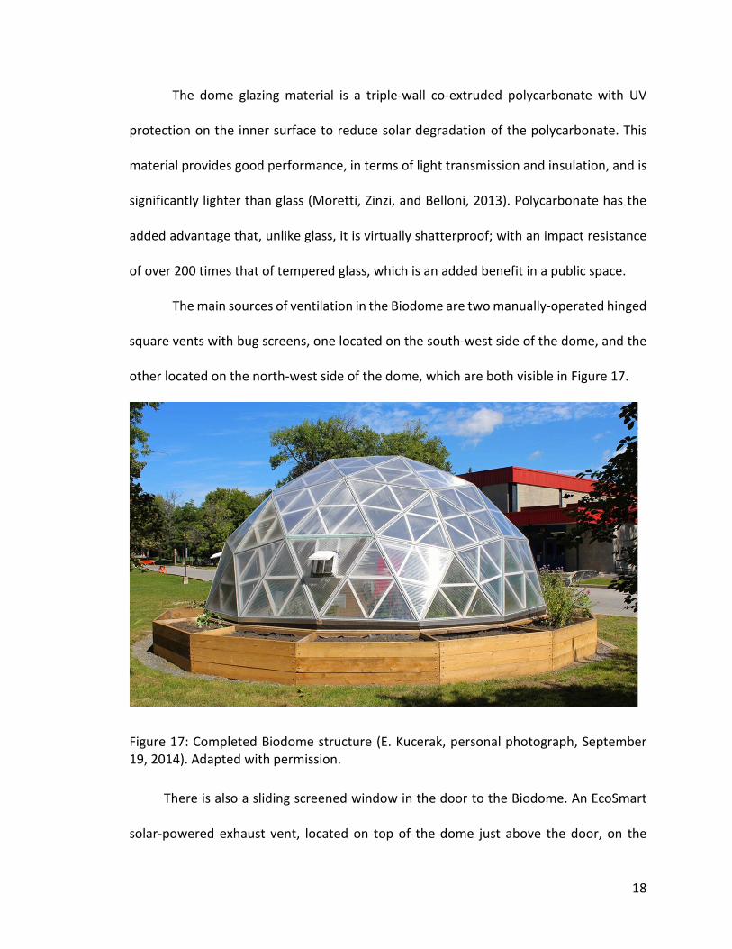
The main sources of ventilation in the Biodome are two manually-operated hinged

square vents with bug screens, one located on the south-west side of the dome, and the

other located on the north-west side of the dome, which are both visible in Figure 17.

Figure 17: Completed Biodome structure (E. Kucerak, personal photograph, September

19, 2014). Adapted with permission.

There is also a sliding screened window in the door to the Biodome. An EcoSmart

solar-powered exhaust vent, located on top of the dome just above the door, on the

19

north-east side, with an integrated solar panel mounted facing south provides forced

ventilation. The exhaust vent has a maximum rated capacity of 500 CFM (0.24 m3/s),

depending on available solar radiation and intake ventilation area (GAF, 2015).

1.3 Research Objectives

The main question to be answered by this research is whether appropriate growing

conditions (to be defined in Chapter 2) can be maintained in the Biodome year-round

without the use of auxiliary power, such as grid-supplied electricity, and without the use

of a supplementary heating source, such as propane, natural gas, or biomass.

The main topics to be included in the scope of work of this project are:

• The effects of solar gain, thermal mass, and insulation on greenhouse air and

soil temperatures;

• The effect of shading by solar photovoltaic panels mounted on the roof of the

Biodome; and

• The measurement and regulation of internal temperature.

Some constraints that will be considered, but not assessed directly include:

• The overall design of greenhouse dome structure and foundation, including

compliance with local building codes;

• The internal design of the greenhouse, including placement of benches,

displays, etc.; and

• Water drainage.

Topics to be specifically excluded from this analysis include:

• The design and maintenance of the aquaculture system, including plant and fish

20

selection and maintenance;

• The design and maintenance of the growing beds, including plant selection,

maintenance, yields, etc.;

• Construction methods; and

• Water supply.

1.4 Organization of Research and Thesis Document

This document is organized as follows:

• Chapter 2 provides a review of literature that is relevant to the research topic.

• Chapter 3 describes the experimental approach and instrumentation including

the development of a TRNSYS model and a data acquisition system.

• Chapter 4 describes the results of the modelled and measured scenarios.

• Chapter 5 provides a comparison and discussion of the scenarios.

• Chapter 6 describes the contributions of this thesis work.

• Chapter 7 provides conclusions on the experimental results as well as

recommendations for future research and possible improvements to both the

Biodome TRNSYS model and the Biodome design and operation.

21

Chapter 2

2

Literature Review

2.1 Introduction

To inform the current research and provide guidance to the Biodome team on design

aspects to include in the construction of the dome, a literature review was conducted and

is presented here. The review begins with a description of greenhouses, including the

optimal growing conditions and the effects of greenhouse shape and orientation on

performance. Geodesic dome greenhouses, in particular, are discussed next, followed by

a description of thermal energy storage systems and their applicability to greenhouse

environmental control.

2.2 Greenhouses

Greenhouses can be considered to be large solar thermal collectors. The transparent

glazing on a greenhouse allows short-wave radiation into the greenhouse where it is

absorbed by surfaces within the dome and re-radiated as long-wave radiation, such as

heat and infrared radiation, that cannot pass back through the glazing. The accumulation

of energy through this greenhouse effect increases the temperature inside the

greenhouse.

2.2.1 Temperature

The optimal temperature inside a greenhouse is heavily dependent on the nature of the

crop being grown. For example, cold-season crops, such as spinach and kale, are more

22

tolerant of low temperatures and may even tolerate brief periods of freezing

temperatures, while tropical, or warm-season crops, such as tomatoes and cucumbers,

would be killed by the same low temperatures. Therefore, it is important to consider the

target crops when designing a greenhouse and, if possible, rotate the crops so that they

align with the growing season.

Cool-season crops tend to do best when grown in the range of 5 to 15.5oC and will

tolerate an occasional drop near 0oC or an increase to 32oC. Warm-season crops tend to

do best when grown in the range of 15.5 to 27oC and will tolerate an occasional drop to

10oC or an increase to 38oC. For most vegetables, very little growth will occur below 5oC

or above 30oC (McCullagh, 1978).

In climates with extreme temperatures in both the summer and winter, both

heating and cooling may be required in order to operate a greenhouse year-round. A

composite system that can be used for both heating and cooling greenhouses is the EAHE,

which is described in further detail in Section 2.4.

According to the American Society of Agricultural and Biological Engineers

(ASABE), most heat loss from a greenhouse is lost through long-wave (thermal) radiation,

conduction, convection, and infiltration (ASABE, 2008), so each of these modes of heat

loss should be addressed in order to maintain an optimum temperature and reduce the

amount of supplementary heat required. An additional heat loss mechanism was

proposed by Rempel et al. (2013) who theorized that glazing cooling due to rain can draw

energy from a greenhouse’s mass, as well as air, through radiative exchange.

The density and type of crop being grown in the greenhouse will also affect the

23

amount of solar energy that is converted to heat. The American Society of Heating,

Refrigeration and Air-Conditioning Engineers (ASHRAE) estimates that in a greenhouse

with a mature crop of plants, one-half of the incoming solar energy is converted to latent

heat, one-quarter to one-third, to sensible heat, and the remainder is either reflected out

of the greenhouse or absorbed by the plants and used in photosynthesis (2011). A

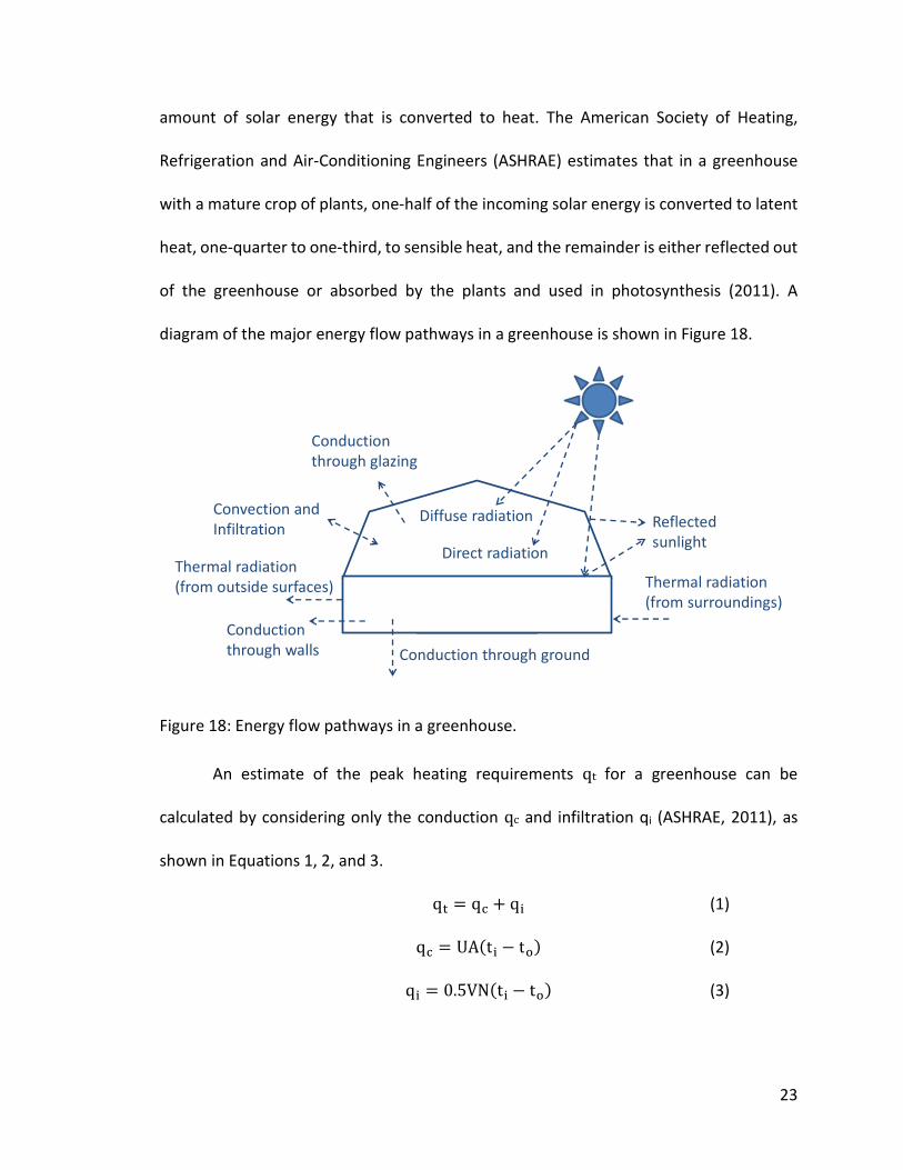
diagram of the major energy flow pathways in a greenhouse is shown in Figure 18.

Figure 18: Energy flow pathways in a greenhouse.

An estimate of the peak heating requirements qt for a greenhouse can be

calculated by considering only the conduction qc and infiltration qi (ASHRAE, 2011), as

shown in Equations 1, 2, and 3.

q� = q� + q� (1)

q� = UA�t� − t�� (2)

q� = 0.5VN�t� − t�� (3)

Conduction

through glazing

Thermal radiation

(from outside surfaces)

Conduction through ground

Thermal radiation

(from surroundings)

Conduction

through walls

Convection and

Infiltration Reflected

sunlight

Diffuse radiation

Direct radiation

24

where: U = overall heat loss coefficient, W/(m2 K)

A = surface area, m2

ti = inside temperature, oC

to = outside temperature, oC

V = greenhouse internal volume, m3

N = number of air changes per hour, h-1

The overall heat loss coefficient U can be estimated based on the type of

construction and the heat transfer coefficient of the glazing material.

Although Equation 1 provides a good estimate of the peak heating load for a greenhouse,

it does not take into account the effect of thermal energy storage, which is discussed in

Section 2.4.

Conduction heat loss occurs mainly between the greenhouse floor and the soil

below, and through the greenhouse glazing (Vadiee, 2011), so this form of heat loss can

be reduced through the use of improved ground insulation and glazing materials with a

high U factor. Unfortunately, a material’s thermal performance is normally inversely

related to its light transmissivity, so the relative importance of these two properties must

be considered for a given climate and growing conditions. It should also be noted that

water condensation on the inside surface of glazing increases the thermal resistance of

the glazing (Zhu et al., 1998).

2.2.2 Lighting

Solar radiation that enters a greenhouse can be categorized as ultraviolet radiation,

photosynthetically active radiation, and near-infrared radiation. Of these three types of

25

solar radiation, only photosynthetically active radiation, which has light wavelengths of

400 to 700 nm, contributes to photosynthesis (Lamnatou and Chemisan, 2012). Light

intensity is also important to plant growth. For example, light saturation (the maximum

level of light intensity a plant is capable of absorbing) of lettuce occurs at 11 MJ/m2 d, and

growth is inhibited at 19 MJ/m2 d (Lamnatou and Chemisan, 2012). Samples of

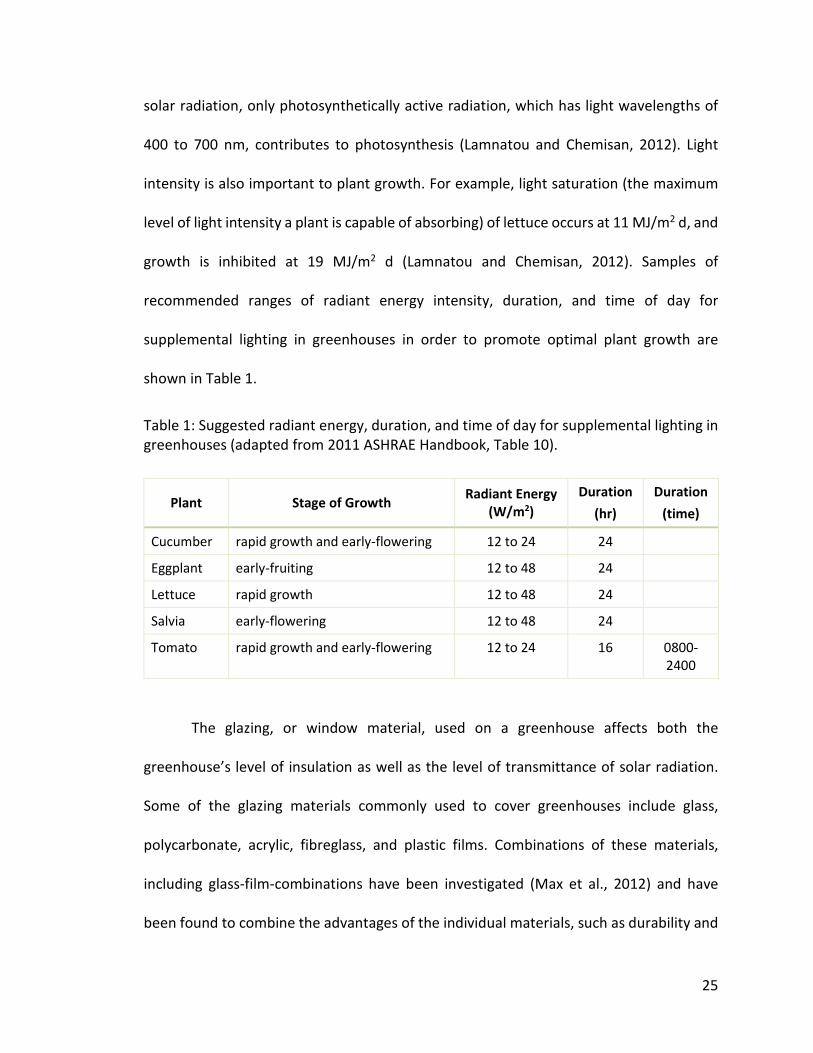
recommended ranges of radiant energy intensity, duration, and time of day for

supplemental lighting in greenhouses in order to promote optimal plant growth are

shown in Table 1.

Table 1: Suggested radiant energy, duration, and time of day for supplemental lighting in

greenhouses (adapted from 2011 ASHRAE Handbook, Table 10).

Plant Stage of Growth Radiant Energy

(W/m2)

Duration

(hr)

Duration

(time)

Cucumber rapid growth and early-flowering 12 to 24 24

Eggplant early-fruiting 12 to 48 24

Lettuce rapid growth 12 to 48 24

Salvia early-flowering 12 to 48 24

Tomato rapid growth and early-flowering 12 to 24 16 0800-

2400

The glazing, or window material, used on a greenhouse affects both the

greenhouse’s level of insulation as well as the level of transmittance of solar radiation.

Some of the glazing materials commonly used to cover greenhouses include glass,

polycarbonate, acrylic, fibreglass, and plastic films. Combinations of these materials,

including glass-film-combinations have been investigated (Max et al., 2012) and have

been found to combine the advantages of the individual materials, such as durability and

26

low weight, and of single and double-layer systems, such as light transmission and

insulation properties. Polycarbonate panels also provide good thermal and optical

performance with a much lower weight than glass, at a similar price (Moretti et al., 2014).

2.2.3 Ventilation and Humidity

Ventilation affects three main variables in a greenhouse: humidity; temperature; and

concentration of CO2. The relative humidity in a greenhouse should be maintained above

40 percent to prevent plant wilt (McCullagh, 1978), but should not be kept higher than

85 percent in order to reduce the risk of the crop developing fungal diseases (Campen et

al., 2003).

Plants require CO2 for photosynthesis and grow best in high CO2 environments.

Ambient air contains about 300 ppm of CO2, while the level of CO2 in a closed greenhouse

may reach 500 ppm at dawn and can quickly drop to less than 200 ppm on a sunny day if

there is insufficient ventilation available, which can lead to reduced growth rates

(Agriculture Canada, 1987).

Ventilation can either be natural or forced. Natural ventilation is accomplished

through the use of strategically placed vent openings in the greenhouse and is dependent

on wind speed and direction, as well as on the temperature differential between the

greenhouse air and ambient air. Forced ventilation involves the use of fans or blowers to

mechanically move air. Fuchs et al. (1997) found that external wind speed has no

significant effects on forced ventilation.

The most effective vent configuration is a combination of roof and side vents,

followed by side vents only, which have a 46% reduction in ventilation, while the least

27

effective vent configuration uses only roof vents and results in a 71% reduction in

ventilation (Katsoulas et al., 2006).

In order to ensure sufficient natural ventilation Agriculture Canada’s (1987)

general guideline is to provide a total ventilation area of at least one-sixth of the

greenhouse floor area, with the total upper area representing about 55% of the total

ventilation area. As noted by Sethi and Sharma (2007) a vent opening area of 15 to

30 percent of greenhouse floor area is recommended, as the effect of additional

ventilation area on the temperature difference is very small above this range.

The use of insect screens in vent openings causes a reduction in natural

greenhouse ventilation rate. Katsoulas et al. (2006) estimated this decrease to be about

33 percent. Decreased screen porosity is associated with decreased ventilation rate and

increased vertical temperature gradients (Sethi and Sharma, 2007). The effect of insect

screens must be taken into consideration when calculating the required ventilation area.

If an aquaculture system is included in the greenhouse, the surface evaporation

of the water in the fish tanks and plant grow beds will also contribute to the relative

humidity and further increase the ventilation requirements, and therefore the overall

energy requirements. To reduce this effect, it is recommended that tank surface openings

be covered at night (Fuller, 2007).

2.2.4 Effects of Greenhouse Shape and Orientation on Performance

Five of the most commonly used single span greenhouse shapes are even-span, uneven-

span, vinery, modified arch, and quonset type (Sethi, 2009). Sethi (2009) modelled and

compared the level of solar radiation, and the resulting inside air temperature, for each

28

of these greenhouse shapes in both an east-west orientation and in a north-west

orientation. Assuming greenhouses of the same size (i.e., same height, width, and length),

Sethi found that the shape and orientation of the greenhouse affected the total solar

radiation incident upon it. Sethi concluded that at altitudes of 31oN, where ambient air

temperatures are low in winter but high in summer, resulting in harsh summers and

winters, a greenhouse shape that receives less radiation in summer (e.g., Quonset shape)

but more in winters (e.g., Uneven-span) would be ideal and an east-west orientation

would be preferred, as it would provide more radiation in winter and less in summer.

As it is not feasible to use two different shapes in one year, Sethi suggested that a

greenhouse that neither receives highest solar radiation in summer nor least solar

radiation in winter would be preferred, such as a modified arch or even-span greenhouse.

In areas where the ambient air temperature remains low during most of the year, Sethi

suggested that a greenhouse shape that received the highest solar radiation throughout

the year, such as the uneven-span greenhouse, should be selected. Unfortunately, no

scientific studies on the relative effectiveness of a geodesic dome greenhouse were found

during the literature review.

2.3 Geodesic Dome Greenhouses

Dome-shaped buildings were made popular in the 1950s by Buckminster “Bucky” Fuller

who named these structures “geodesic domes”, inspired by the term “geodesic line”,

which refers to the shortest distance between two points on a curved surface (Chandler,

2015).

29

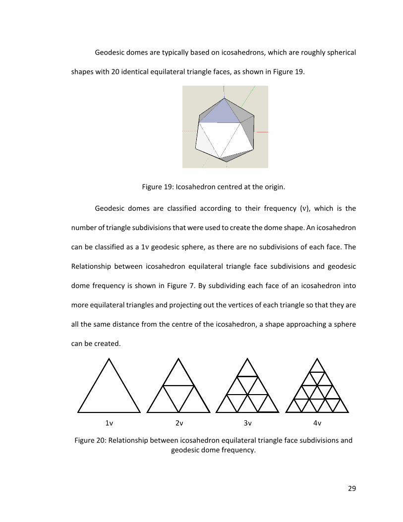
Geodesic domes are typically based on icosahedrons, which are roughly spherical

shapes with 20 identical equilateral triangle faces, as shown in Figure 19.

Figure 19: Icosahedron centred at the origin.

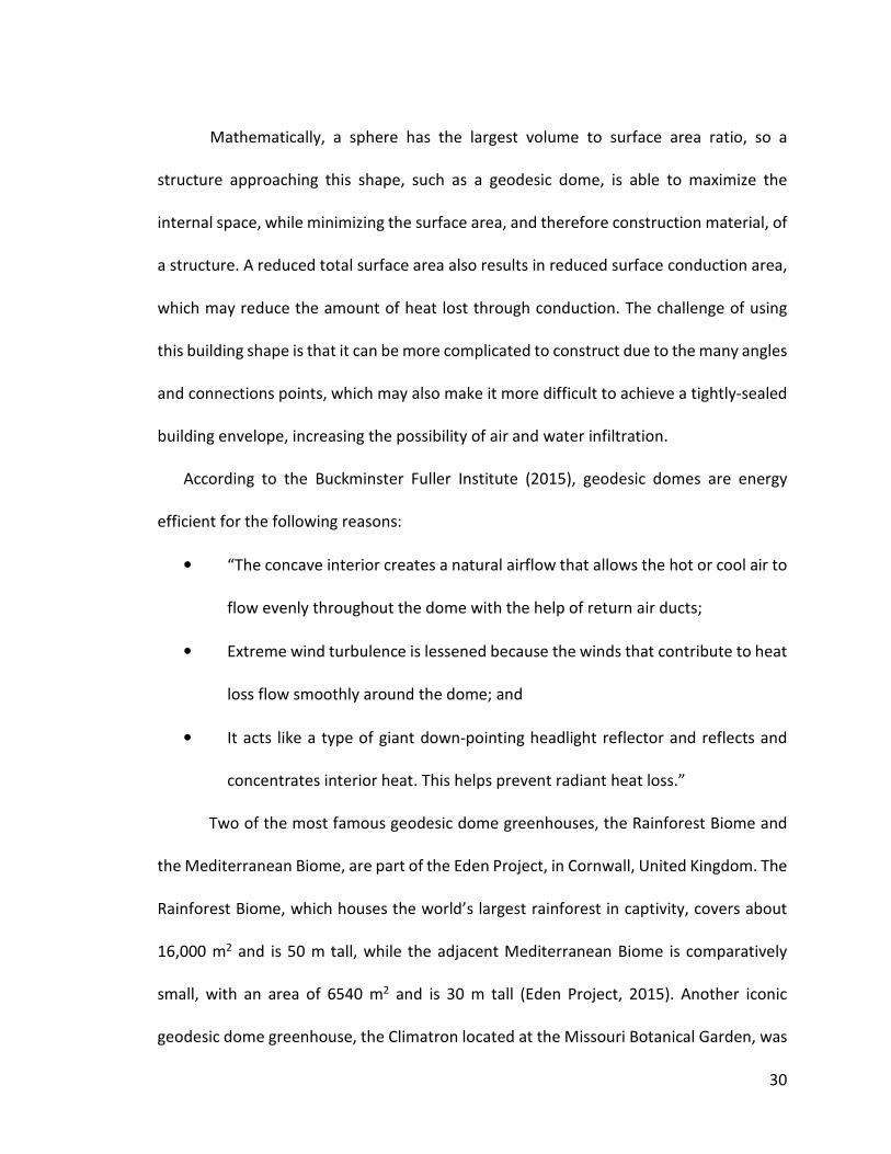
Geodesic domes are classified according to their frequency (v), which is the

number of triangle subdivisions that were used to create the dome shape. An icosahedron

can be classified as a 1v geodesic sphere, as there are no subdivisions of each face. The

Relationship between icosahedron equilateral triangle face subdivisions and geodesic

dome frequency is shown in Figure 7. By subdividing each face of an icosahedron into

more equilateral triangles and projecting out the vertices of each triangle so that they are

all the same distance from the centre of the icosahedron, a shape approaching a sphere

can be created.

Figure 20: Relationship between icosahedron equilateral triangle face subdivisions and

geodesic dome frequency.

30

Mathematically, a sphere has the largest volume to surface area ratio, so a

structure approaching this shape, such as a geodesic dome, is able to maximize the

internal space, while minimizing the surface area, and therefore construction material, of

a structure. A reduced total surface area also results in reduced surface conduction area,

which may reduce the amount of heat lost through conduction. The challenge of using

this building shape is that it can be more complicated to construct due to the many angles

and connections points, which may also make it more difficult to achieve a tightly-sealed

building envelope, increasing the possibility of air and water infiltration.

According to the Buckminster Fuller Institute (2015), geodesic domes are energy

efficient for the following reasons:

• “The concave interior creates a natural airflow that allows the hot or cool air to

flow evenly throughout the dome with the help of return air ducts;

• Extreme wind turbulence is lessened because the winds that contribute to heat

loss flow smoothly around the dome; and

• It acts like a type of giant down-pointing headlight reflector and reflects and

concentrates interior heat. This helps prevent radiant heat loss.”

Two of the most famous geodesic dome greenhouses, the Rainforest Biome and

the Mediterranean Biome, are part of the Eden Project, in Cornwall, United Kingdom. The

Rainforest Biome, which houses the world’s largest rainforest in captivity, covers about

16,000 m2 and is 50 m tall, while the adjacent Mediterranean Biome is comparatively

small, with an area of 6540 m2 and is 30 m tall (Eden Project, 2015). Another iconic

geodesic dome greenhouse, the Climatron located at the Missouri Botanical Garden, was

31

built in 1960 as the first geodesic dome to be used as a conservatory (Missouri Botanical

Garden, 2015). The Climatron covers more than 2000 m2, has a centre height of over

21 m, and spans over 53 m at its base. Individual and community-sized dome greenhouses

are also becoming increasingly popular, with several manufacturers and individuals

constructing domes all over the world.

Although there is a lot of anecdotal evidence available on the internet on the

effectiveness of geodesic domes as greenhouses, very little scientific data on this topic

was found through a search of scholarly sources. Various attempts were made to contact

owners, operators, and builders of other geodesic dome greenhouses, but no useful

information was collected. A representative at Growing Spaces indicated that over the

years they had collected a “decent amount of data” but that it was not well organized (U.

Parsons, personal communication, June 12, 2015).

The only reference to a geodesic dome greenhouse in the literature was by

Provenzano and Winfield (1987) who used a geodesic dome greenhouse with

polyethylene glazing to cover a tilapia growth tank measuring 10.7 m3 and reported that

the fish tank water temperatures generally remained between 24 and 36oC between May

and September in Virginia, USA, with an average daily fresh water make-up rate of

4 percent of tank volume.

2.4 Thermal Energy Storage

In a typical commercial greenhouse, air temperature is primarily controlled using a

combination of shading, misting, and ventilation for cooling, and some form of auxiliary

heater for heating. Solar greenhouses are instead designed to maximize the capture and

32

storage of solar energy in thermal mass and minimize heat loss through insulation,

resulting in reduced daily temperature fluctuations and reduced heating and cooling

requirements. Thermal energy that is captured, stored, and later released without the use

of any outside energy, such as electricity to drive fan or pump, is considered to have

undergone passive thermal storage. If at any point during the process outside energy is

used to capture, store, or release the thermal energy, then that portion of the system is

considered to involve active thermal storage. Santamouris et al. (1994) identified five

main categories of passive solar greenhouse, according to the characteristics of the heat

storage system, namely, water, latent heat material, rock bed, buried pipes, and other.

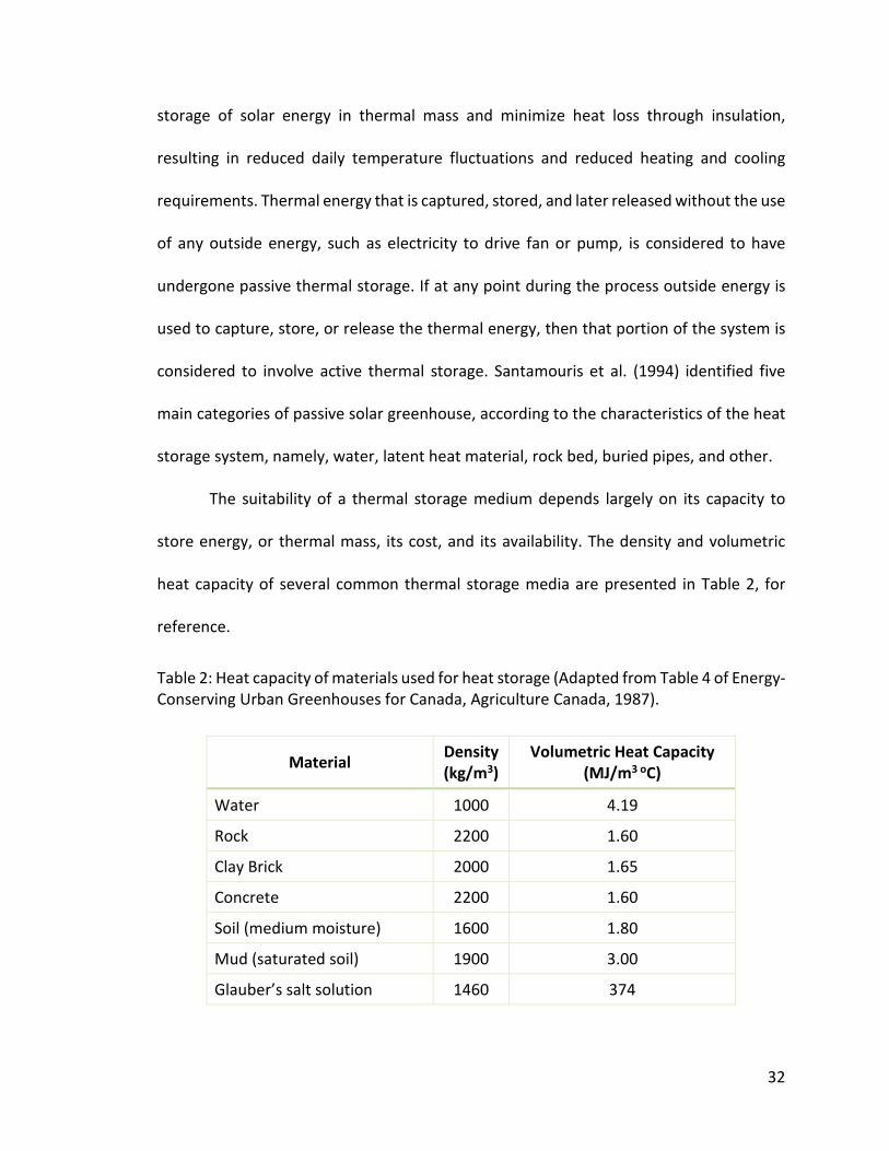
The suitability of a thermal storage medium depends largely on its capacity to

store energy, or thermal mass, its cost, and its availability. The density and volumetric

heat capacity of several common thermal storage media are presented in Table 2, for

reference.

Table 2: Heat capacity of materials used for heat storage (Adapted from Table 4 of Energy-

Conserving Urban Greenhouses for Canada, Agriculture Canada, 1987).

Material Density

(kg/m3)

Volumetric Heat Capacity

(MJ/m3 oC)

Water 1000 4.19

Rock 2200 1.60

Clay Brick 2000 1.65

Concrete 2200 1.60

Soil (medium moisture) 1600 1.80

Mud (saturated soil) 1900 3.00

Glauber’s salt solution 1460 374

33

Sethi and Sharma (2008) compiled a comprehensive survey and evaluation of

greenhouse heating energy storage technologies, including water storage, rock bed

storage, phase change material storage, and earth-to-air heat exchanger systems. The

benefits and challenges of each of these types of thermal storage system and guidelines

on the quantity of storage material required are discussed in the following four sections.

2.4.1 Water Thermal Energy Storage

As was shown in Table 2, water has a volumetric heat capacity that is almost three times

greater than that of rock, clay brick, and concrete at about half the density, making it an

effective thermal storage material. Water is also relatively inexpensive and is generally

readily available. One challenge of using water as a thermal energy storage medium is

that it has the potential to freeze when exposed to prolonged sub-zero temperatures and

upon freezing it may expand enough to damage its storage container, which may lead to

water leaks that can be very destructive, depending on the environment they are in.

Water tanks placed in a greenhouse also occupy precious floor space that could instead

be using for cultivation.

Gupta and Tiwari (2002) created a model for predicting the thermal storage effect

of water mass in a greenhouse. Their transient model predicted room air temperature,

storage water temperature, and the thermal energy storage effect of a water mass in a

passive greenhouse. Their conclusions are that there is a significant thermal energy

storage effect of a large water mass on the internal greenhouse air temperature, as

evidenced by the decrease in thermal load leveling that is associated with an increase in

the mass of storage water. Similarly, Zhu et al. (1998) modelled the thermal

34

characteristics of greenhouse pond systems in TRNSYS and found that the night time air

temperature in a greenhouse with a pond remains a few degrees higher than in a similar

greenhouse.

Sethi and Sharma (2008) developed empirical relationships between the volume

of water storage and greenhouse floor area, listed in Table 3, to provide greenhouse

designers with a method of estimating the approximate volume of water storage required

for a given application.

Table 3: Empirical relationships between water storage volumes used for given


from Table 2 in Sethi and Sharma, 2008).

Type Empirical relationship a rrrr2222 �r�r�r�rxyxyxyxy��

Greenhouse ground area versus volume

of water storage used (overall)

Yw = 0.0362X + 1.1005 0.7731 0.879

Polyethylene as cover material Yw = 0.037X + 0.6071 0.827 0.909

Glass as cover material Yw = 0.0699X - 1.5449 0.6048 0.777

Ground tubes as storage material Yw = 0.0232X + 1.8865 0.4175 0.646

Water tanks/barrels as storage material Yw = 0.0369X + 1.9042 0.8875 0.942

a Yw represents the volume of water storage in kl, X represents the greenhouse floor area

in m2.

It should be noted that these relationships were developed based on other

researchers’ reported water volumes and greenhouse floor areas, but these volumes

were not necessarily optimized for the given situations and may not reflect best practices.

These equations also ignore the effects of greenhouse location, volume, crop, etc.

Nonetheless, these equations can provide a starting point for future work.

35

2.4.2 Rock Bed Thermal Energy Storage

Heat can be stored in a rock bed thermal energy storage system either passively or

actively. In passive systems, heat is stored in the rock bed during the day through direct

incident solar radiation and is released at night through convection, once the indoor air

temperature falls below that of the rock bed. In active systems, fans are used to blow air

through the rock bed. During the day, warm air is pushed through the rock bed to remove

excess heat from the air and charge the rock bed and at night the cooler indoor air is

pushed in reverse through the rock bed to be reheated. Although a very large quantity of

rock is required for an effective rock bed storage system, it does not have to occupy

internal floor space, as the rock bed can be built underneath or adjacent to the

greenhouse.

Sethi and Sharma (2008) developed empirical relationships between the heat

capacity of rock bed storage and greenhouse ground areas using different cover materials

and storage material, listed in Table 4, to provide greenhouse designers with a method of

estimating the approximate heat storage capacity required for a given greenhouse

application. They found that rock beds are typically composed of 2 to 10 cm diameter

gravel with a depth of 40 to 50 cm and can satisfy 20 to 70 percent of a greenhouse’s

annual heating needs, with inside temperatures ranging from 4 to 10oC higher than

minimum ambient air temperatures.

36

Table 4: Empirical relationships between heat capacity of rock bed storage and


from Table 4 in Sethi and Sharma, 2008).

Type Empirical relationship a rrrr2222 �r�r�r�rxyxyxyxy��

Greenhouse ground area versus heat

capacity of rock storage used (overall)

Yr = 0.0362X + 1.1005 0.7731 0.879

Polyethylene as cover material Yr = 0.037X + 0.6071 0.827 0.909

Glass as cover material Yr = 0.0699X - 1.5449 0.6048 0.777

Gravel as storage material Yr = 0.0232X + 1.8865 0.4175 0.646

a Yr = heat capacity of rock storage in kJ/oC, X = greenhouse floor area in m2

2.4.3 Earth-to-Air Heat Exchangers

Earth-to-air heat exchangers (EAHE) provide another method of storing energy in the

ground under or adjacent to a greenhouse or other building. In these systems fans are

used to circulate the naturally warm, moist air of the greenhouse underground through

pipes in order to transfer the heat to the underground thermal mass, which can include

sand, soil, rocks, or a combination of these materials. In the case of the Biodome, fans

located at the air intake box will be used to push warm greenhouse air through the pipes

buried under the internal garden beds and out through the two air outlet boxes located

within the Biodome, as described in Section 1.2. The warm air will heat the soil

surrounding the pipes in the EAHE system.

Ghosal and Tiwari (2006) reported that the use of an EAHE was found to result in

greenhouse air temperatures that were on average 7 to 8oC higher in the winter and 5 to

6oC lower in the summer than in the same greenhouse without an EAHE. They also found

that the EAHE was increasingly effective with increasing pipe length, decreasing pipe

37

diameter, decreasing mass flow rate of flowing air and increasing depths up to 4 m.

Unfortunately, no optimization of the combination of these variables was performed and

no upper limits were stated, other than the limit of 4 m of depth.

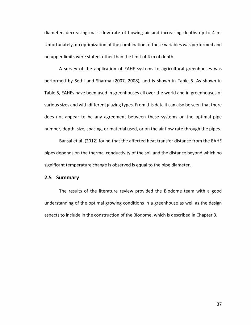
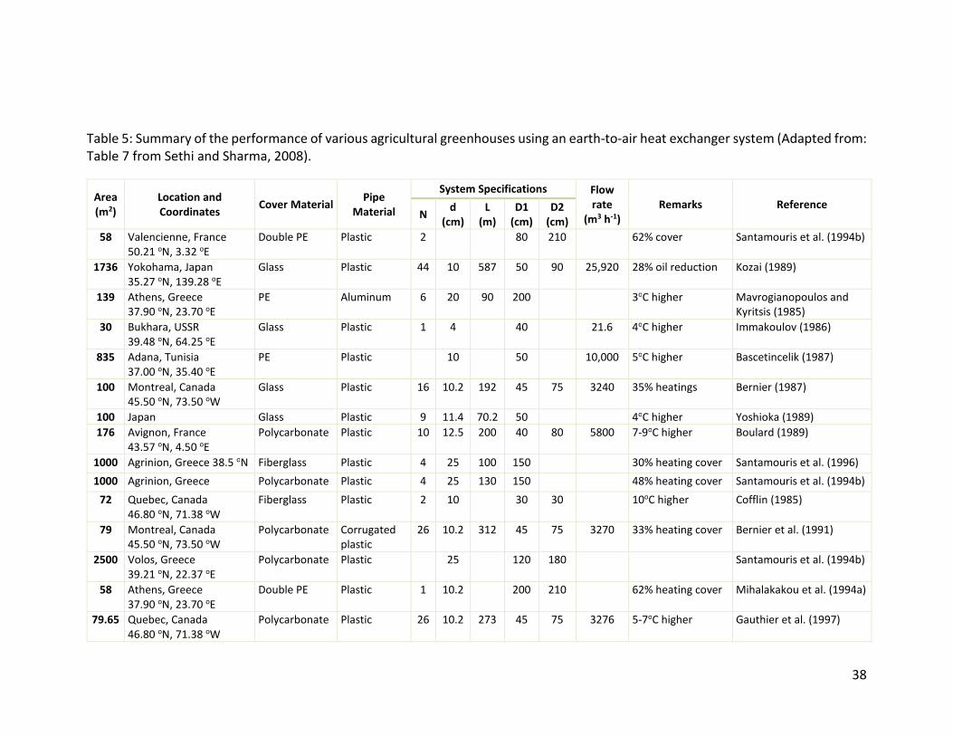
A survey of the application of EAHE systems to agricultural greenhouses was

performed by Sethi and Sharma (2007, 2008), and is shown in Table 5. As shown in

Table 5, EAHEs have been used in greenhouses all over the world and in greenhouses of

various sizes and with different glazing types. From this data it can also be seen that there

does not appear to be any agreement between these systems on the optimal pipe

number, depth, size, spacing, or material used, or on the air flow rate through the pipes.

Bansal et al. (2012) found that the affected heat transfer distance from the EAHE

pipes depends on the thermal conductivity of the soil and the distance beyond which no

significant temperature change is observed is equal to the pipe diameter.

2.5 Summary

The results of the literature review provided the Biodome team with a good

understanding of the optimal growing conditions in a greenhouse as well as the design

aspects to include in the construction of the Biodome, which is described in Chapter 3.

38

Table 5: Summary of the performance of various agricultural greenhouses using an earth-to-air heat exchanger system (Adapted from:

Table 7 from Sethi and Sharma, 2008).

Area

(m2)

Location and

Coordinates Cover Material

Pipe

Material

System Specifications Flow

rate

(m3 h-1)

Remarks Reference N

d

(cm)

L

(m)

D1

(cm)

D2

(cm)

58 Valencienne, France

50.21 oN, 3.32 oE

Double PE Plastic 2 80 210 62% cover Santamouris et al. (1994b)

1736 Yokohama, Japan

35.27 oN, 139.28 oE

Glass Plastic 44 10 587 50 90 25,920 28% oil reduction Kozai (1989)

139 Athens, Greece

37.90 oN, 23.70 oE

PE Aluminum 6 20 90 200 3oC higher Mavrogianopoulos and

Kyritsis (1985)

30 Bukhara, USSR

39.48 oN, 64.25 oE

Glass Plastic 1 4 40 21.6 4oC higher Immakoulov (1986)

835 Adana, Tunisia

37.00 oN, 35.40 oE

PE Plastic 10 50 10,000 5oC higher Bascetincelik (1987)

100 Montreal, Canada

45.50 oN, 73.50 oW

Glass Plastic 16 10.2 192 45 75 3240 35% heatings Bernier (1987)

100 Japan Glass Plastic 9 11.4 70.2 50 4oC higher Yoshioka (1989)

176 Avignon, France

43.57 oN, 4.50 oE

Polycarbonate Plastic 10 12.5 200 40 80 5800 7-9oC higher Boulard (1989)

1000 Agrinion, Greece 38.5 oN Fiberglass Plastic 4 25 100 150 30% heating cover Santamouris et al. (1996)

1000 Agrinion, Greece Polycarbonate Plastic 4 25 130 150 48% heating cover Santamouris et al. (1994b)

72 Quebec, Canada

46.80 oN, 71.38 oW

Fiberglass Plastic 2 10 30 30 10oC higher Cofflin (1985)

79 Montreal, Canada

45.50 oN, 73.50 oW

Polycarbonate Corrugated

plastic

26 10.2 312 45 75 3270 33% heating cover Bernier et al. (1991)

2500 Volos, Greece

39.21 oN, 22.37 oE

Polycarbonate Plastic 25 120 180 Santamouris et al. (1994b)

58 Athens, Greece

37.90 oN, 23.70 oE

Double PE Plastic 1 10.2 200 210 62% heating cover Mihalakakou et al. (1994a)

79.65 Quebec, Canada

46.80 oN, 71.38 oW

Polycarbonate Plastic 26 10.2 273 45 75 3276 5-7oC higher Gauthier et al. (1997)

39

Chapter 3

3

Modelling and Experimental Approach and Instrumentation

3.1 Introduction

This section describes: the experimental approach that was taken to evaluate the effects

of ventilation, water thank thermal storage, and solar panel shading on the Biodome

operating conditions, the modelling approach used to simulate the performance of the

Biodome, the design and implementation of the instrumentation and control system,

including a detailed description of the system so that this system can be used in future

projects, the instrumentation plan, and the model calibration approach.

3.2 Experimental Approach

In order to test the effects of ventilation, water tank thermal mass, and solar panel

shading on both the modelled and the measured results, different combinations of these

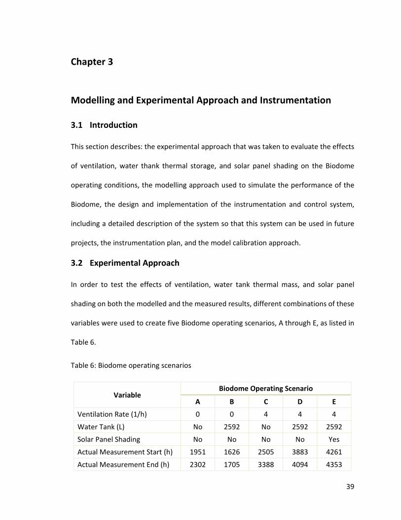
variables were used to create five Biodome operating scenarios, A through E, as listed in

Table 6.

Table 6: Biodome operating scenarios

Variable Biodome Operating Scenario

A B C D E

Ventilation Rate (1/h) 0 0 4 4 4

Water Tank (L) No 2592 No 2592 2592

Solar Panel Shading No No No No Yes

Actual Measurement Start (h) 1951 1626 2505 3883 4261

Actual Measurement End (h) 2302 1705 3388 4094 4353

40

The ventilation rate could not be modulated, due to the nature of the ventilation

system, so the effects of ventilation were studied by turning the ventilation on and off.

The appropriate volume of water thermal storage to be used in the Biodome was

calculated using Equation 4, from Table 3 of the literature review, shown below, which

results in a recommended total tank volume of 3,377 L.

Yw = 0.0369X + 1.9042 (4)

where: Yw represents the volume of water storage (kL)

X represents the greenhouse floor area (m2)

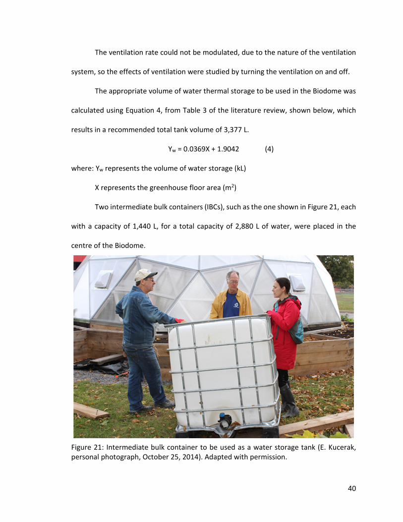
Two intermediate bulk containers (IBCs), such as the one shown in Figure 21, each

with a capacity of 1,440 L, for a total capacity of 2,880 L of water, were placed in the

centre of the Biodome.

Figure 21: Intermediate bulk container to be used as a water storage tank (E. Kucerak,

personal photograph, October 25, 2014). Adapted with permission.

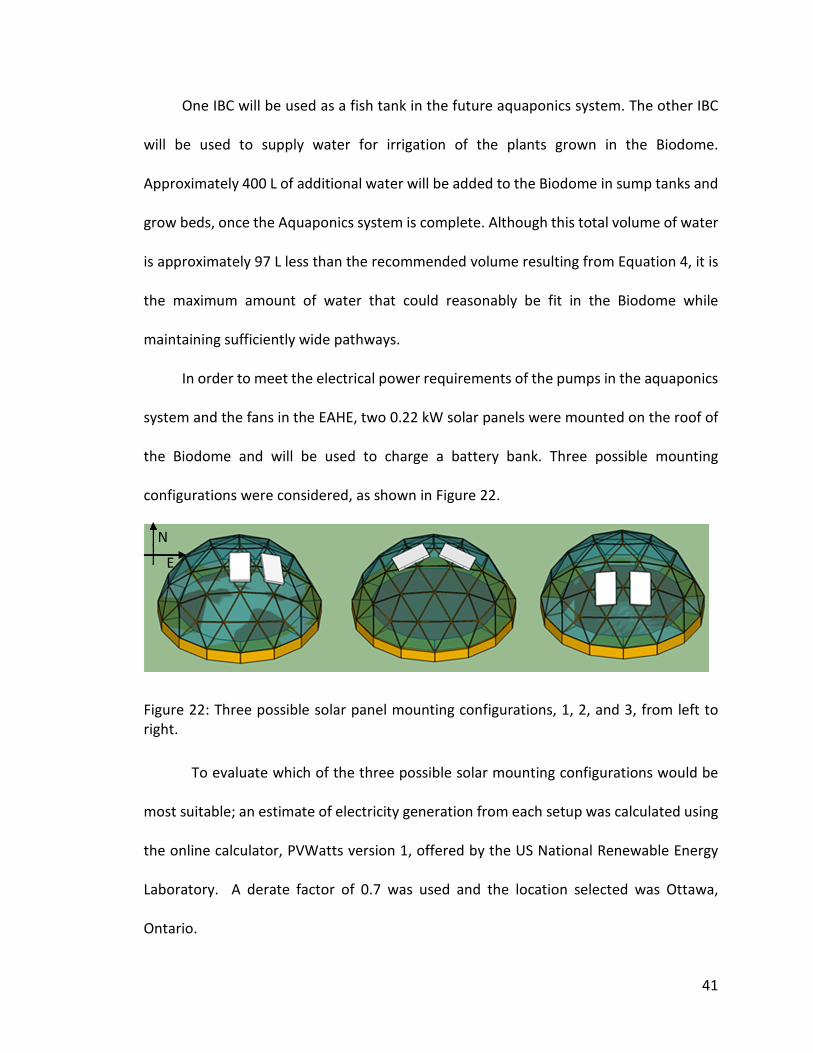
41

One IBC will be used as a fish tank in the future aquaponics system. The other IBC

will be used to supply water for irrigation of the plants grown in the Biodome.

Approximately 400 L of additional water will be added to the Biodome in sump tanks and

grow beds, once the Aquaponics system is complete. Although this total volume of water

is approximately 97 L less than the recommended volume resulting from Equation 4, it is

the maximum amount of water that could reasonably be fit in the Biodome while

maintaining sufficiently wide pathways.

In order to meet the electrical power requirements of the pumps in the aquaponics

system and the fans in the EAHE, two 0.22 kW solar panels were mounted on the roof of

the Biodome and will be used to charge a battery bank. Three possible mounting

configurations were considered, as shown in Figure 22.

Figure 22: Three possible solar panel mounting configurations, 1, 2, and 3, from left to

right.

To evaluate which of the three possible solar mounting configurations would be

most suitable; an estimate of electricity generation from each setup was calculated using

the online calculator, PVWatts version 1, offered by the US National Renewable Energy

Laboratory. A derate factor of 0.7 was used and the location selected was Ottawa,

Ontario.

N

E

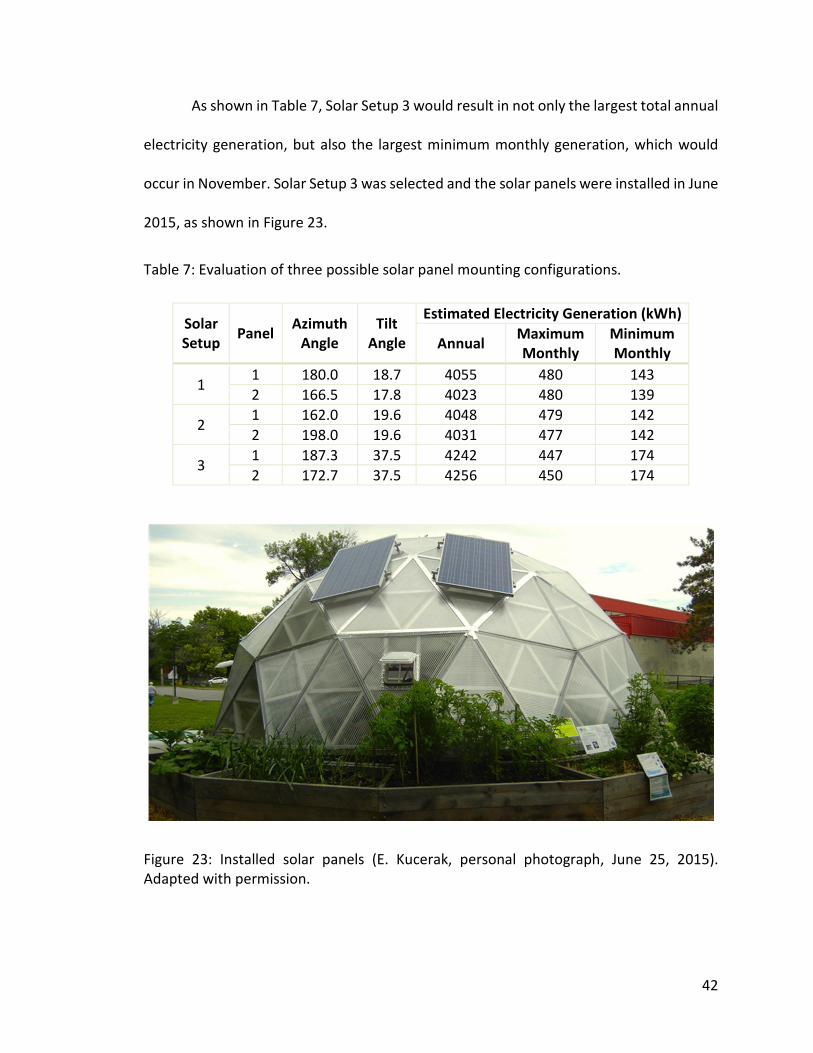
42

As shown in Table 7, Solar Setup 3 would result in not only the largest total annual

electricity generation, but also the largest minimum monthly generation, which would

occur in November. Solar Setup 3 was selected and the solar panels were installed in June

2015, as shown in Figure 23.

Table 7: Evaluation of three possible solar panel mounting configurations.

Solar

Setup Panel

Azimuth

Angle

Tilt

Angle

Estimated Electricity Generation (kWh)

Annual Maximum

Monthly

Minimum

Monthly

1 1 180.0 18.7 4055 480 143

2 166.5 17.8 4023 480 139

2 1 162.0 19.6 4048 479 142

2 198.0 19.6 4031 477 142

3 1 187.3 37.5 4242 447 174

2 172.7 37.5 4256 450 174

Figure 23: Installed solar panels (E. Kucerak, personal photograph, June 25, 2015).

Adapted with permission.

43

3.3 Modelling Approach

The modelling approach of this thesis relies on the development and use of a TRNSYS

model. The TRNSYS software package is a transient system simulation program that can

be used to evaluate many different types of transient systems, such as solar thermal

systems, multizone buildings, cogeneration systems, etc. A TRNSYS project is composed

of connected components, known as Types, which are each described by a mathematical

model in the TRNSYS simulation engine (TRNSYS, 2012). An additional tool, TRNBuild, is

used to enter input data for multizone buildings, such building structure details, window

optical properties, heating and cooling schedules, etc. (TRNSYS, 2012).

The TRNSYS modelling platform was used because it has a proven record for

accurately modelling greenhouses. It has been used by many researchers to create

greenhouse models (Fuller et al., 1987; Willits et al., 1985; Fuller, 2007; Vadiee, 2011;

Hollmuller and Lachal, 1998; Hoes and Desmedt, 2008; Wong et al., 2011).

The main components of the Biodome TRNSYS model are: Type 15-5, weather data

reading and processing; Type 56, multi-zone building model; calculators, specifically

Wizard Settings, Azimuth Angles, and Radiation calculators; and printers, specifically the

Irradiation, Temperature, and System printers.

Each of these components is shown in the TRNSYS model in Figure 24 and is

described in the sections below. The complete TRNSYS input file is provided in

Appendix A and the TRNSYS deck file is provided in Appendix B.

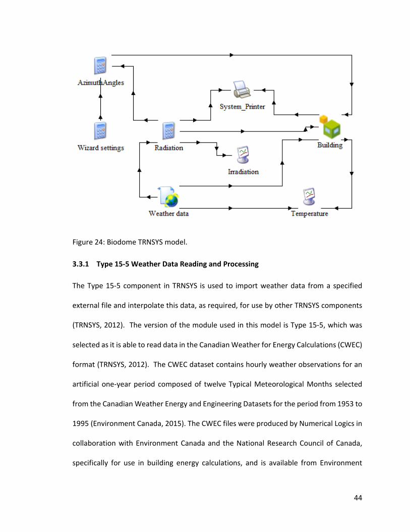
44

Figure 24: Biodome TRNSYS model.

3.3.1 Type 15-5 Weather Data Reading and Processing

The Type 15-5 component in TRNSYS is used to import weather data from a specified

external file and interpolate this data, as required, for use by other TRNSYS components

(TRNSYS, 2012). The version of the module used in this model is Type 15-5, which was

selected as it is able to read data in the Canadian Weather for Energy Calculations (CWEC)

format (TRNSYS, 2012). The CWEC dataset contains hourly weather observations for an

artificial one-year period composed of twelve Typical Meteorological Months selected

from the Canadian Weather Energy and Engineering Datasets for the period from 1953 to

1995 (Environment Canada, 2015). The CWEC files were produced by Numerical Logics in

collaboration with Environment Canada and the National Research Council of Canada,

specifically for use in building energy calculations, and is available from Environment

45

Canada (2015). The CWEC files follow the ASHRAE Weather Year for Energy Calculation 2

format. The CWEC file used for the simulations in this project is composed of data from

the following weather station (Environment Canada, 2015):

• Station Name: Ottawa International Airport

• Latitude: 45.32

• Longitude: -75.67

• Elevation: 114 m

• World Meteorological Organization Identifier: 716280

In order to develop a file of actual weather data to be used for model comparison

and calibration, the CWEC file described above was used as the starting point and actual

data for 2015 was substituted, where applicable and available, as described below.

Carleton University is host to a Campbell Scientific Weather Station, which is

mounted on the roof of the Mackenzie Building and automatically measures and logs data

every 5 minutes. For the period from January 1, 2015 to July 1, 2015, the CWEC data was

replaced with weather data collected by this weather station for the following fields: dry

bulb temperature (oC); relative humidity (%); global horizontal radiation (Wh/m2); wind

direction (degrees); and wind speed (m/s).

All atmospheric pressure data for this time period was taken from the Ottawa CDA

RCS (Canada Department of Agriculture Reference Climate Station) weather station,

available online from Environment Canada (2015). The details of this weather station are

as follows (Environment Canada, 2015):

46

• Station Name: OTTAWA CDA RCS

• Latitude: 45.38

• Longitude: -75.72

• Elevation: 79.2 m

• Climate Reference Identifier: 6105978

• World Meteorological Organization Identifier: 71063

• International Air Transport Association/ Transport Canada Identifier: XOA

The Carleton weather station was not functional from February 13, 2015 to

February 25, 2015, so the data for this period is taken from the Ottawa CDA RCS weather

station (Environment Canada, 2015) instead. For the period from July 1 to December 31,

CWEC data is used as a placeholder for all fields.

Weather variables that were not used in calculations affecting the models were

left unchanged, including extraterrestrial horizontal radiation (Wh/m2), extraterrestrial

direct normal radiation (Wh/m2), direct normal radiation, diffuse horizontal radiation,

global horizontal, direct normal, and diffuse horizontal illuminance (lux), zenith luminance

(Cd/m2), total sky cover (0.1), and opaque sky cover (0.1).

Minor data cleaning was done to prevent calculation errors, including removing

all non-zero values from the global horizontal radiation field for periods before or after

sunrise or sunset, respectively and removing all zero atmospheric pressure readings and

replacing these values with the values from the previous non-zero pressure reading.

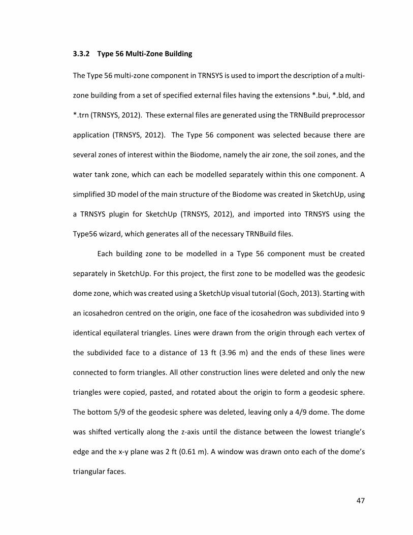
47

3.3.2 Type 56 Multi-Zone Building

The Type 56 multi-zone component in TRNSYS is used to import the description of a multi-

zone building from a set of specified external files having the extensions *.bui, *.bld, and

*.trn (TRNSYS, 2012). These external files are generated using the TRNBuild preprocessor

application (TRNSYS, 2012). The Type 56 component was selected because there are

several zones of interest within the Biodome, namely the air zone, the soil zones, and the

water tank zone, which can each be modelled separately within this one component. A

simplified 3D model of the main structure of the Biodome was created in SketchUp, using

a TRNSYS plugin for SketchUp (TRNSYS, 2012), and imported into TRNSYS using the

Type56 wizard, which generates all of the necessary TRNBuild files.

Each building zone to be modelled in a Type 56 component must be created

separately in SketchUp. For this project, the first zone to be modelled was the geodesic

dome zone, which was created using a SketchUp visual tutorial (Goch, 2013). Starting with

an icosahedron centred on the origin, one face of the icosahedron was subdivided into 9

identical equilateral triangles. Lines were drawn from the origin through each vertex of

the subdivided face to a distance of 13 ft (3.96 m) and the ends of these lines were

connected to form triangles. All other construction lines were deleted and only the new

triangles were copied, pasted, and rotated about the origin to form a geodesic sphere.

The bottom 5/9 of the geodesic sphere was deleted, leaving only a 4/9 dome. The dome

was shifted vertically along the z-axis until the distance between the lowest triangle’s

edge and the x-y plane was 2 ft (0.61 m). A window was drawn onto each of the dome’s

triangular faces.

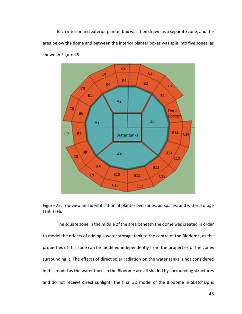
48

Each interior and exterior planter box was then drawn as a separate zone, and the

area below the dome and between the interior planter boxes was split into five zones, as

shown in Figure 25.

Figure 25: Top-view and identification of planter bed zones, air spaces, and water storage

tank area.

The square zone in the middle of the area beneath the dome was created in order

to model the effects of adding a water storage tank to the centre of the Biodome, as the

properties of this zone can be modified independently from the properties of the zones

surrounding it. The effects of direct solar radiation on the water tanks is not considered

in this model as the water tanks in the Biodome are all shaded by surrounding structures

and do not receive direct sunlight. The final 3D model of the Biodome in SketchUp is

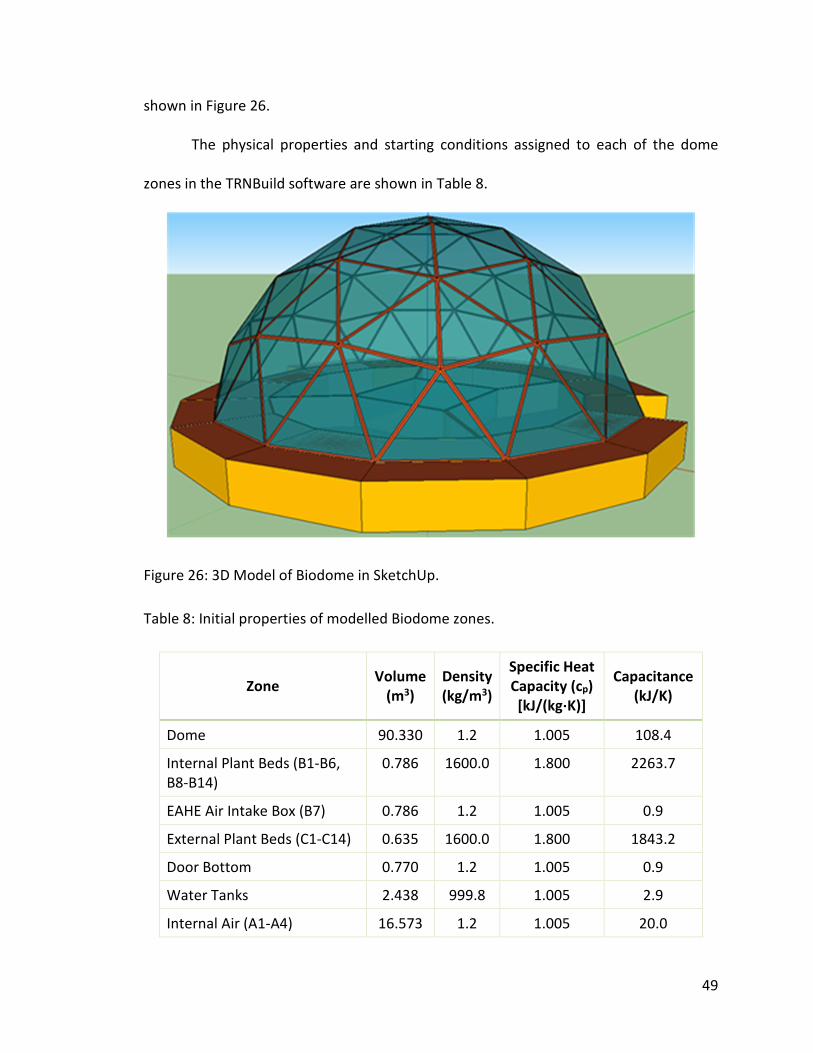
49

shown in Figure 26.

The physical properties and starting conditions assigned to each of the dome

zones in the TRNBuild software are shown in Table 8.

Figure 26: 3D Model of Biodome in SketchUp.

Table 8: Initial properties of modelled Biodome zones.

Zone Volume

(m3)

Density

(kg/m3)

Specific Heat

Capacity (cp)

[kJ/(kg⋅⋅⋅⋅K)]

Capacitance

(kJ/K)

Dome 90.330 1.2 1.005 108.4

Internal Plant Beds (B1-B6,

B8-B14)

0.786 1600.0 1.800 2263.7

EAHE Air Intake Box (B7) 0.786 1.2 1.005 0.9

External Plant Beds (C1-C14) 0.635 1600.0 1.800 1843.2

Door Bottom 0.770 1.2 1.005 0.9

Water Tanks 2.438 999.8 1.005 2.9

Internal Air (A1-A4) 16.573 1.2 1.005 20.0

50

The volumes for most of the zones were read from the SketchUp file, except for

the water tank volume, which was calculated based on the size of the two intermediate

bulk containers used, assuming they are filled to 90 percent of their total capacity. The

volumes of the internal plant beds were all made equal in order to facilitate manual

changes to capacitance values in future model runs. The density and specific heat capacity

of each zone was based on the properties of the material in each zone. For example, it

was assumed that the internal and external plant beds would be filled with soil and the

water tank would be filled with water. The capacitance of each zone was calculated by

multiplying the volume, density, and specific heat capacity. The specific heat capacity of

the Water Tank zone was set to that of air in order to represent an empty water tank. The

starting temperature and humidity of each zone was set to 0oC and 95 percent relative

humidity, respectively.

The dome glazing is 16 mm triple-wall polycarbonate structured sheet (PCSS),

produced by Polygal. The relevant technical data for the PCSS provided by Polygal (2011)

is as follows:

• Gauge: 16 mm (5/8”)

• Light Transmission: 70% (according to ASTM D1003)

• U-Factor: 0.41 Btu∙h-1∙ft-2∙F-1 (0.71 W∙m-2∙K-1)

• R-Factor: 2.439 Btu∙h-1∙ft-1∙F-1 (4.221 W∙m-1∙K-1)

• Shading Coefficient: 0.790

• Solar Heat Gain Coefficient (SHGC): 0.680

• Solar Reflection: 0.223

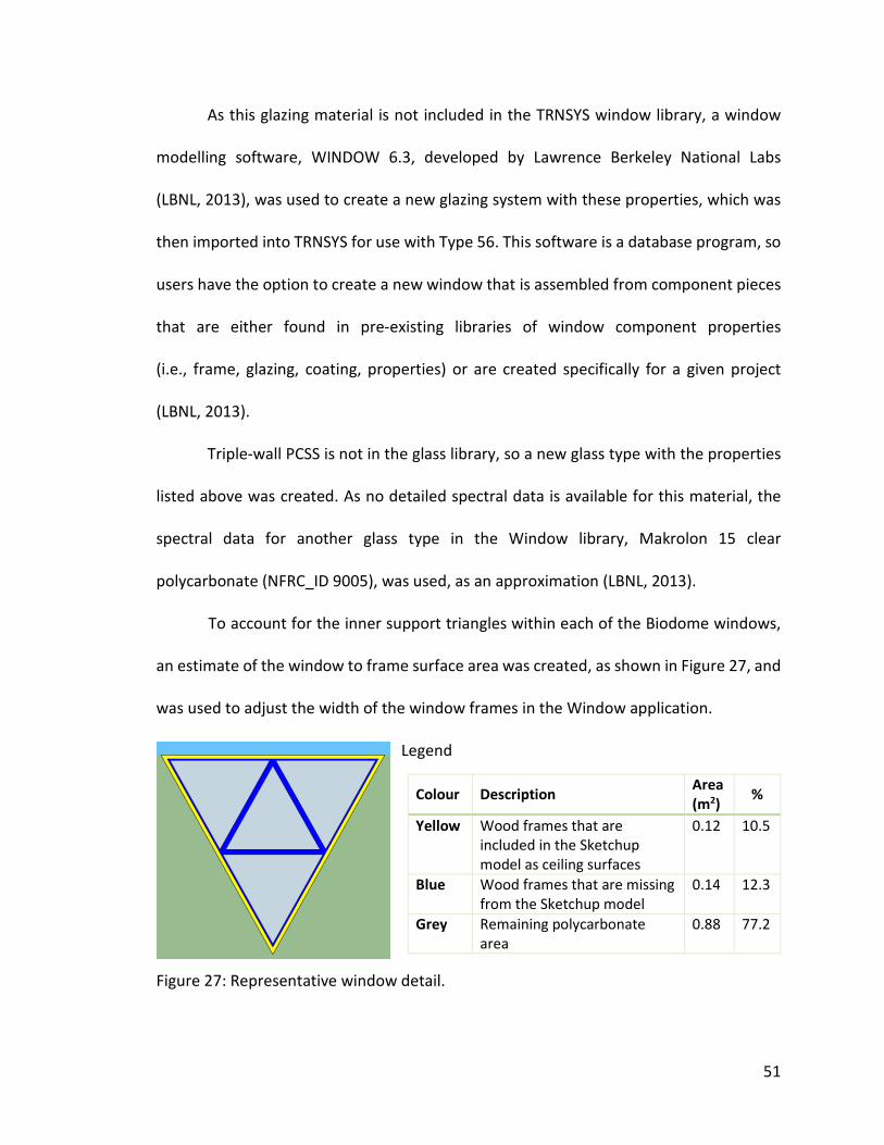
51

As this glazing material is not included in the TRNSYS window library, a window

modelling software, WINDOW 6.3, developed by Lawrence Berkeley National Labs

(LBNL, 2013), was used to create a new glazing system with these properties, which was

then imported into TRNSYS for use with Type 56. This software is a database program, so

users have the option to create a new window that is assembled from component pieces

that are either found in pre-existing libraries of window component properties

(i.e., frame, glazing, coating, properties) or are created specifically for a given project

(LBNL, 2013).

Triple-wall PCSS is not in the glass library, so a new glass type with the properties

listed above was created. As no detailed spectral data is available for this material, the

spectral data for another glass type in the Window library, Makrolon 15 clear

polycarbonate (NFRC_ID 9005), was used, as an approximation (LBNL, 2013).

To account for the inner support triangles within each of the Biodome windows,

an estimate of the window to frame surface area was created, as shown in Figure 27, and

was used to adjust the width of the window frames in the Window application.

Legend

Figure 27: Representative window detail.

Colour Description Area

(m2) %

Yellow Wood frames that are

included in the Sketchup

model as ceiling surfaces

0.12 10.5

Blue Wood frames that are missing

from the Sketchup model

0.14 12.3

Grey Remaining polycarbonate

area

0.88 77.2

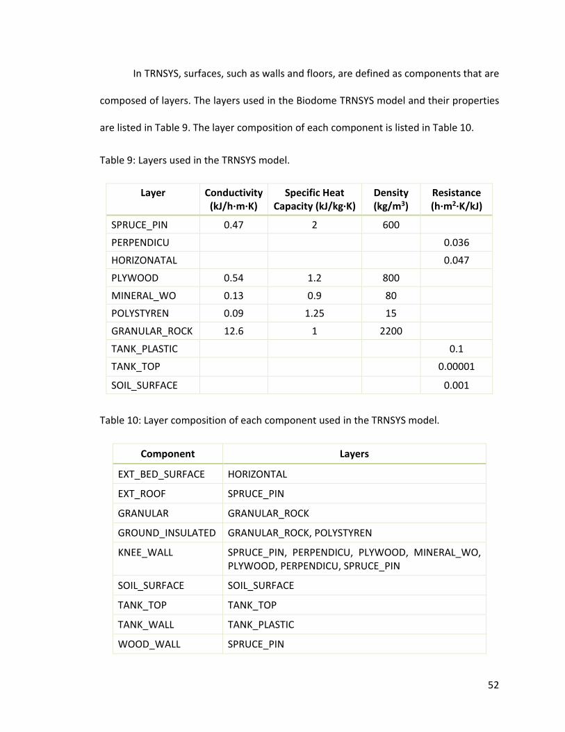
52

In TRNSYS, surfaces, such as walls and floors, are defined as components that are

composed of layers. The layers used in the Biodome TRNSYS model and their properties

are listed in Table 9. The layer composition of each component is listed in Table 10.

Table 9: Layers used in the TRNSYS model.

Layer Conductivity

(kJ/h·m·K)

Specific Heat

Capacity (kJ/kg·K)

Density

(kg/m3)

Resistance

(h·m2·K/kJ)

SPRUCE_PIN 0.47 2 600

PERPENDICU 0.036

HORIZONATAL 0.047

PLYWOOD 0.54 1.2 800

MINERAL_WO 0.13 0.9 80

POLYSTYREN 0.09 1.25 15

GRANULAR_ROCK 12.6 1 2200

TANK_PLASTIC 0.1

TANK_TOP 0.00001

SOIL_SURFACE 0.001

Table 10: Layer composition of each component used in the TRNSYS model.

Component Layers

EXT_BED_SURFACE HORIZONTAL

EXT_ROOF SPRUCE_PIN

GRANULAR GRANULAR_ROCK

GROUND_INSULATED GRANULAR_ROCK, POLYSTYREN

KNEE_WALL SPRUCE_PIN, PERPENDICU, PLYWOOD, MINERAL_WO,

PLYWOOD, PERPENDICU, SPRUCE_PIN

SOIL_SURFACE SOIL_SURFACE

TANK_TOP TANK_TOP

TANK_WALL TANK_PLASTIC

WOOD_WALL SPRUCE_PIN

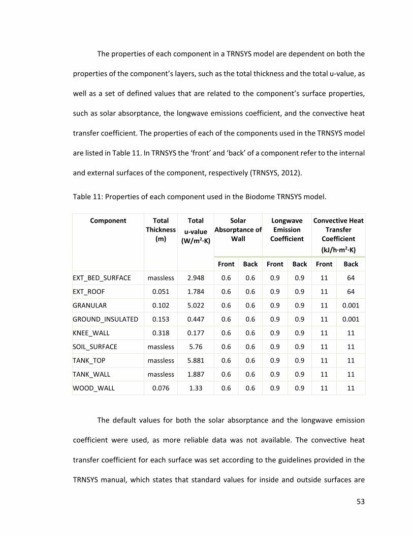
53

The properties of each component in a TRNSYS model are dependent on both the

properties of the component’s layers, such as the total thickness and the total u-value, as

well as a set of defined values that are related to the component’s surface properties,

such as solar absorptance, the longwave emissions coefficient, and the convective heat

transfer coefficient. The properties of each of the components used in the TRNSYS model

are listed in Table 11. In TRNSYS the ‘front’ and ‘back’ of a component refer to the internal

and external surfaces of the component, respectively (TRNSYS, 2012).

Table 11: Properties of each component used in the Biodome TRNSYS model.

Component

Total

Thickness

(m)

Total

u-value

(W/m2·K)

Solar

Absorptance of

Wall

Longwave

Emission

Coefficient

Convective Heat

Transfer

Coefficient

(kJ/h·m2·K)

Front Back Front Back Front Back

EXT_BED_SURFACE massless 2.948 0.6 0.6 0.9 0.9 11 64

EXT_ROOF 0.051 1.784 0.6 0.6 0.9 0.9 11 64

GRANULAR 0.102 5.022 0.6 0.6 0.9 0.9 11 0.001

GROUND_INSULATED 0.153 0.447 0.6 0.6 0.9 0.9 11 0.001

KNEE_WALL 0.318 0.177 0.6 0.6 0.9 0.9 11 11

SOIL_SURFACE massless 5.76 0.6 0.6 0.9 0.9 11 11

TANK_TOP massless 5.881 0.6 0.6 0.9 0.9 11 11

TANK_WALL massless 1.887 0.6 0.6 0.9 0.9 11 11

WOOD_WALL 0.076 1.33 0.6 0.6 0.9 0.9 11 11

The default values for both the solar absorptance and the longwave emission

coefficient were used, as more reliable data was not available. The convective heat

transfer coefficient for each surface was set according to the guidelines provided in the

TRNSYS manual, which states that standard values for inside and outside surfaces are

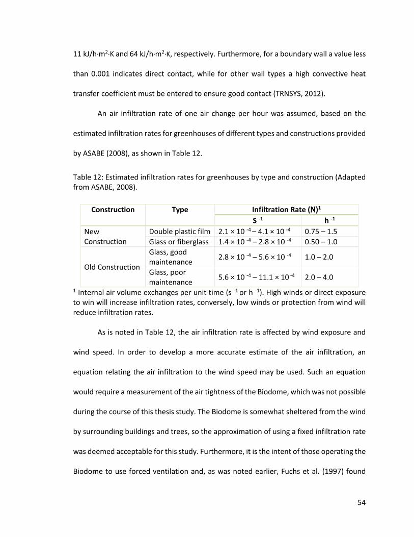
54

11 kJ/h∙m2∙K and 64 kJ/h∙m2∙K, respectively. Furthermore, for a boundary wall a value less

than 0.001 indicates direct contact, while for other wall types a high convective heat

transfer coefficient must be entered to ensure good contact (TRNSYS, 2012).

An air infiltration rate of one air change per hour was assumed, based on the

estimated infiltration rates for greenhouses of different types and constructions provided

by ASABE (2008), as shown in Table 12.

Table 12: Estimated infiltration rates for greenhouses by type and construction (Adapted

from ASABE, 2008).

Construction Type Infiltration Rate (NNNN)1

S -1 h -1

New

Construction

Double plastic film 2.1 × 10 -4 – 4.1 × 10 -4 0.75 – 1.5

Glass or fiberglass 1.4 × 10 -4 – 2.8 × 10 -4 0.50 – 1.0

Old Construction

Glass, good

maintenance 2.8 × 10 -4 – 5.6 × 10 -4 1.0 – 2.0

Glass, poor

maintenance 5.6 × 10 -4 – 11.1 × 10 -4 2.0 – 4.0

1 Internal air volume exchanges per unit time (s -1 or h -1). High winds or direct exposure

to win will increase infiltration rates, conversely, low winds or protection from wind will

reduce infiltration rates.

As is noted in Table 12, the air infiltration rate is affected by wind exposure and

wind speed. In order to develop a more accurate estimate of the air infiltration, an

equation relating the air infiltration to the wind speed may be used. Such an equation

would require a measurement of the air tightness of the Biodome, which was not possible

during the course of this thesis study. The Biodome is somewhat sheltered from the wind

by surrounding buildings and trees, so the approximation of using a fixed infiltration rate

was deemed acceptable for this study. Furthermore, it is the intent of those operating the

Biodome to use forced ventilation and, as was noted earlier, Fuchs et al. (1997) found

55

that external wind speed has no significant effects on forced ventilation.

The Biodome is equipped with forced ventilation in the form of one solar powered

exhaust ventilation fan with a maximum rated capacity of 500 cfm (0.24 m3/s), depending

on available solar radiation and intake ventilation area (GAF, 2015). The internal air

volume of the Biodome is approximately 100 m3, therefore the fan should provide a

maximum of 8.6 air changes per hour. Given the fact that the ventilation intake area is

limited, each of the openings is covered in a bug screen, and the solar panel will not

always produce its maximum rated output, the ventilation rate was modelled as

4 air changes per hour, in addition to the 1 air change per hour due to infiltration. The

fan’s on/off control was modelled so that the fan is on whenever there is incident solar

radiation in the plane of the solar panel, which faces south, with an approximate tilt of

50o, and off when there is none.

The coupling air flow rate between the Dome zone and each of the Internal Air

zones (A1-A4) and the Door Bottom zone was set to 5000 kg/h in order to ensure

complete internal air mixing.

3.3.3 Calculators

There are three calculators used in the TRNSYS model, Wizard settings, Azimuth Angles,

and Radiation, which are each described below.

The Wizard setting calculator was automatically generated when the 3D model

was imported from Sketchup using the Multi-Zone Building Model Wizard. This calculator

can be used to adjust the orientation of the Biodome by rotating it about the z-axis

according to a defined number of degrees. There are no inputs to this calculator. The only

56

output from this calculator is to provide the Azimuth Angles calculator with the pre-

defined number of degrees by which to rotate the Type 56 building.

The Azimuth Angles calculator is used to automatically calculate the azimuth

angles of each of the surfaces in the model.

The Radiation calculator is used to calculate the amount of solar radiation incident

on each of the surfaces in the model. The Radiation calculator is also used to turn on and

off the ventilation according to whether where is any incident solar radiation in the plane

of the exhaust vent’s integrated solar panel.

3.3.4 Printers

There are three printers used in the TRNSYS model, Irradiation, Temperature, and System

Printer. The Irradiation printer is automatically generated by the Multi-Zone Building

Model Wizard. It is used to display a graph of the irradiation level on a given surface while

the model is running. This data is not written to a file for future use. The Temperature

printer is also automatically generated by the Multi-Zone Building Model Wizard and is

similar to the Irradiation printer in that it is also used to display a graph of the temperature

of a given zone while the model is running. This data is also not written to a file for future

use. The system printer used in this model is Type25a. The system printer is used to log

model results to a text file for a given set of data points for each time step in the model.

In this model, the system printer is recording the air temperature of the dome, the soil

temperature of the internal and external plant beds, and the temperature of the water

tanks, each in one-hour time steps. This data can be retrieved after the model run is

complete and can be used to do further data analysis.

57

3.4 Instrumentation and Control System

The main criteria in the design of the instrumentation and control system is that it be

easily replicable and customizable for future projects, so all selected components must

be readily accessible and affordable. The system must also be as energy efficient as

possible, given the limited access to electricity and reliance on battery power.

A microcontroller, the Arduino UNO, is used as the data collection device. A

microcontroller was chosen over a microcomputer because of its relative simplicity. A

microcontroller is a single-chip microcomputer with on-board program ROM and

programmable in/out pins, while a microcomputer uses a microprocessor, internal

memory, and storage space to execute applications. The effect of this difference in

architecture is that a microcontroller is only able to execute one program, which is

programmed into the in/out pins, and it does not have the ability to perform data

processing. A microcomputer is essentially a small personal computer and has all of the

same capabilities and requirements, including the need to install an operating system,

which may increase the difficulty of diagnosing problems, should they arise, and may also

increase the required power consumption. Since there is no requirement in this project

for data processing to be co-located with the sensors, as all data processing can be done

remotely, a microcontroller is sufficient for this application.

With the rise in popularity and the drop in price of microcomputers and

microcontrollers, there are now thousands of options available, both from both online

retailers as well as electronics hobby shops, making the selection of an appropriate

solution more difficult. Ultimately the Arduino UNO was selected because of its relative

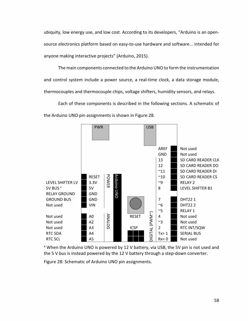
58

ubiquity, low energy use, and low cost. According to its developers, “Arduino is an open-

source electronics platform based on easy-to-use hardware and software... intended for

anyone making interactive projects” (Arduino, 2015).

The main components connected to the Arduino UNO to form the instrumentation

and control system include a power source, a real-time clock, a data storage module,

thermocouples and thermocouple chips, voltage shifters, humidity sensors, and relays.

Each of these components is described in the following sections. A schematic of

the Arduino UNO pin assignments is shown in Figure 28.

PWR USB

AREF Not used

GND Not used

DIG

ITA

L (P

WM

~)

13 SD CARD READER CLK

12 SD CARD READER DO

~11 SD CARD READER DI

RESET

PO

WE

R

Ard

uin

o U

NO

~10 SD CARD READER CS

LEVEL SHIFTER LV 3.3V ~9 RELAY 2

5V BUS a 5V 8 LEVEL SHIFTER B1

RELAY GROUND GND

GROUND BUS GND 7 DHT22 1

Not used VIN ~6 DHT22 2

~5 RELAY 1

Not used A0

AN

ALO

G

RESET 4 Not used

Not used A2 ~3 Not used

Not used A3 ICSP 2 RTC INT/SQW

RTC SDA A4 Tx> 1 SERIAL BUS

RTC SCL A5 Rx< 0 Not used

a When the Arduino UNO is powered by 12 V battery, via USB, the 5V pin is not used and

the 5 V bus is instead powered by the 12 V battery through a step-down converter.

Figure 28: Schematic of Arduino UNO pin assignments.

59

3.4.1 Power

While actively reading data, the Arduino UNO was measured to have a current draw of

approximately 50 mA and this stage lasts approximately three seconds. For the remainder

of the 5 minute cycle between readings, the Arduino UNO was measured to have a

current draw of approximately 29 mA, so the average current is approximately 29.2 mA,

which at a voltage of 5 V means the Arduino requires 0.15 W of power, or 3.6 Wh of

energy per day. Battery capacity is normally given in units of Ah, so the Arduino UNO

would require a 5 V battery with a minimum capacity of about 700 mAh to run for

24 hours. During the initial testing phases, four 1.2 V rechargeable AA batteries with a

capacity of 2500 mAh were used as the power source for the Arduino UNO and were

connected via the barrel socket power input (PWR in Figure 28). These batteries were

typically able to last just over 3 days before being recharged.

During the attempted EAHE fan tests the Arduino UNO was powered by the same

12 V batteries that were used to run the fans. A step-down converter was used to convert

the 12 V source to a steady 3.3 V source that was connected to the Arduino UNO via the

USB port (USB in Figure 28). Ultimately, the Arduino UNO will be connected to the 12 V

batteries being charged by the solar panels, but as of November 2015 this system was not

yet functional, so temporary solutions were implemented for the purposes of this study.

3.4.2 Real-Time Clock

The Arduino UNO does not have an integrated real-time clock (RTC), so it is only able to

use an internal counter to calculate elapsed time. This method of calculating time is

inaccurate and limited by the maximum number on the counter. Additionally, it cannot

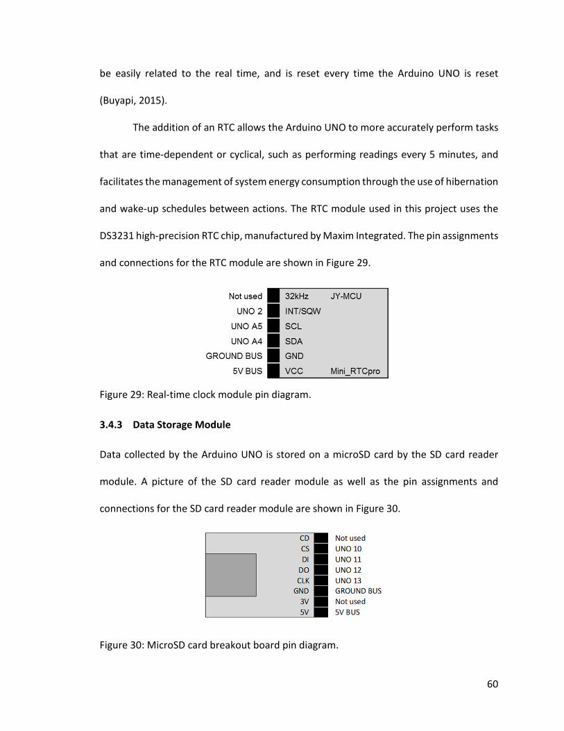
60

be easily related to the real time, and is reset every time the Arduino UNO is reset

(Buyapi, 2015).

The addition of an RTC allows the Arduino UNO to more accurately perform tasks

that are time-dependent or cyclical, such as performing readings every 5 minutes, and

facilitates the management of system energy consumption through the use of hibernation

and wake-up schedules between actions. The RTC module used in this project uses the

DS3231 high-precision RTC chip, manufactured by Maxim Integrated. The pin assignments

and connections for the RTC module are shown in Figure 29.

Figure 29: Real-time clock module pin diagram.

3.4.3 Data Storage Module

Data collected by the Arduino UNO is stored on a microSD card by the SD card reader

module. A picture of the SD card reader module as well as the pin assignments and

connections for the SD card reader module are shown in Figure 30.

Figure 30: MicroSD card breakout board pin diagram.

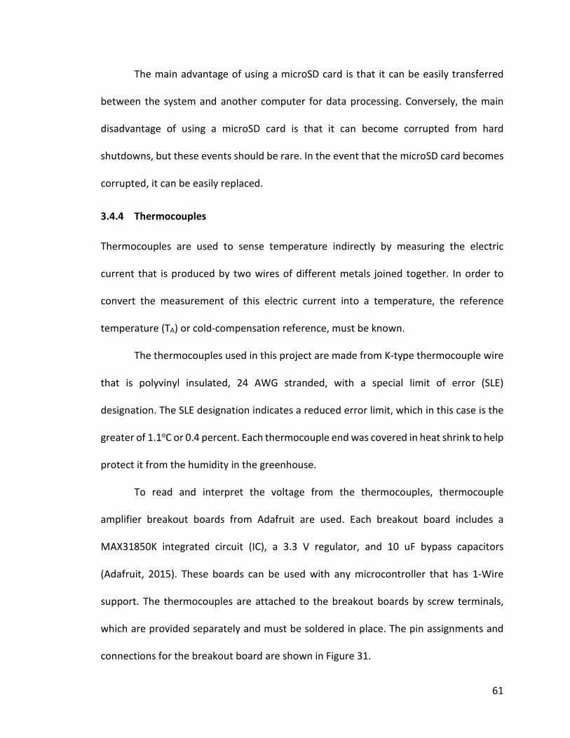
61

The main advantage of using a microSD card is that it can be easily transferred

between the system and another computer for data processing. Conversely, the main

disadvantage of using a microSD card is that it can become corrupted from hard

shutdowns, but these events should be rare. In the event that the microSD card becomes

corrupted, it can be easily replaced.

3.4.4 Thermocouples

Thermocouples are used to sense temperature indirectly by measuring the electric

current that is produced by two wires of different metals joined together. In order to

convert the measurement of this electric current into a temperature, the reference

temperature (TA) or cold-compensation reference, must be known.

The thermocouples used in this project are made from K-type thermocouple wire

that is polyvinyl insulated, 24 AWG stranded, with a special limit of error (SLE)

designation. The SLE designation indicates a reduced error limit, which in this case is the

greater of 1.1oC or 0.4 percent. Each thermocouple end was covered in heat shrink to help

protect it from the humidity in the greenhouse.

To read and interpret the voltage from the thermocouples, thermocouple

amplifier breakout boards from Adafruit are used. Each breakout board includes a

MAX31850K integrated circuit (IC), a 3.3 V regulator, and 10 uF bypass capacitors

(Adafruit, 2015). These boards can be used with any microcontroller that has 1-Wire

support. The thermocouples are attached to the breakout boards by screw terminals,

which are provided separately and must be soldered in place. The pin assignments and

connections for the breakout board are shown in Figure 31.

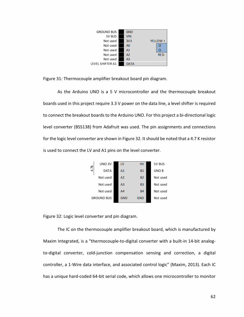
62

Figure 31: Thermocouple amplifier breakout board pin diagram.

As the Arduino UNO is a 5 V microcontroller and the thermocouple breakout

boards used in this project require 3.3 V power on the data line, a level shifter is required

to connect the breakout boards to the Arduino UNO. For this project a bi-directional logic

level converter (BSS138) from Adafruit was used. The pin assignments and connections

for the logic level converter are shown in Figure 32. It should be noted that a 4.7 K resistor

is used to connect the LV and A1 pins on the level converter.

Figure 32: Logic level converter and pin diagram.

The IC on the thermocouple amplifier breakout board, which is manufactured by

Maxim Integrated, is a “thermocouple-to-digital converter with a built-in 14-bit analog-

to-digital converter, cold-junction compensation sensing and correction, a digital

controller, a 1-Wire data interface, and associated control logic” (Maxim, 2013). Each IC

has a unique hard-coded 64-bit serial code, which allows one microcontroller to monitor

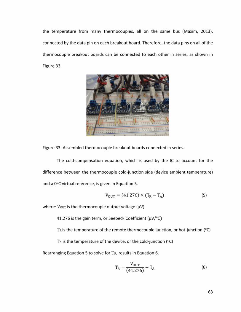
63

the temperature from many thermocouples, all on the same bus (Maxim, 2013),

connected by the data pin on each breakout board. Therefore, the data pins on all of the

thermocouple breakout boards can be connected to each other in series, as shown in

Figure 33.

Figure 33: Assembled thermocouple breakout boards connected in series.

The cold-compensation equation, which is used by the IC to account for the

difference between the thermocouple cold-junction side (device ambient temperature)

and a 0oC virtual reference, is given in Equation 5.

V"#$ � �41.276� ) �T* � T+� (5)

where: VOUT is the thermocouple output voltage (µV)

41.276 is the gain term, or Seebeck Coefficient (µV/℃�

TR is the temperature of the remote thermocouple junction, or hot-junction (oC)

TA is the temperature of the device, or the cold-junction (oC)

Rearranging Equation 5 to solve for TR, results in Equation 6.

T* �

V"#$

�41.276�� T+ (6)

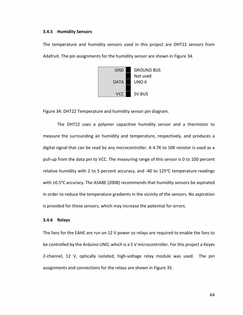
64

3.4.5 Humidity Sensors

The temperature and humidity sensors used in this project are DHT22 sensors from

Adafruit. The pin assignments for the humidity sensor are shown in Figure 34.

Figure 34: DHT22 Temperature and humidity sensor pin diagram.

The DHT22 uses a polymer capacitive humidity sensor and a thermistor to

measure the surrounding air humidity and temperature, respectively, and produces a

digital signal that can be read by any microcontroller. A 4.7K to 10K resistor is used as a

pull-up from the data pin to VCC. The measuring range of this sensor is 0 to 100 percent

relative humidity with 2 to 5 percent accuracy, and -40 to 125oC temperature readings

with ±0.5oC accuracy. The ASABE (2008) recommends that humidity sensors be aspirated

in order to reduce the temperature gradients in the vicinity of the sensors. No aspiration

is provided for these sensors, which may increase the potential for errors.

3.4.6 Relays

The fans for the EAHE are run on 12 V power so relays are required to enable the fans to

be controlled by the Arduino UNO, which is a 5 V microcontroller. For this project a Keyes

2-channel, 12 V, optically isolated, high-voltage relay module was used. The pin

assignments and connections for the relays are shown in Figure 35.

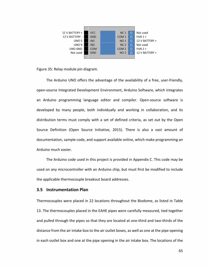
65

Figure 35: Relay module pin diagram.

The Arduino UNO offers the advantage of the availability of a free, user-friendly,

open-source Integrated Development Environment, Arduino Software, which integrates

an Arduino programming language editor and compiler. Open-source software is

developed by many people, both individually and working in collaboration, and its

distribution terms must comply with a set of defined criteria, as set out by the Open

Source Definition (Open Source Initiative, 2015). There is also a vast amount of

documentation, sample code, and support available online, which make programming an

Arduino much easier.

The Arduino code used in this project is provided in Appendix C. This code may be

used on any microcontroller with an Arduino chip, but must first be modified to include

the applicable thermocouple breakout board addresses.

3.5 Instrumentation Plan

Thermocouples were placed in 22 locations throughout the Biodome, as listed in Table

13. The thermocouples placed in the EAHE pipes were carefully measured, tied together

and pulled through the pipes so that they are located at one-third and two-thirds of the

distance from the air intake box to the air outlet boxes, as well as one at the pipe opening

in each outlet box and one at the pipe opening in the air intake box. The locations of the

66

thermocouples in the EAHE pipes were selected in order to measure the difference in

temperature between pipes as well as the temperature gradient across the length of each

pipe. Once installation of the solar panel battery charging system is complete and it

becomes possible to power the fans in the EAHE system and perform experiments on the

operation of the EAHE system, the distribution of thermocouples throughout the EAHE

pipes will be important to characterize the heat transfer gradient across the length of the

pipes.

Table 13: Thermocouple locations.

Thermocouple Locations

1/3 of pipe 1 1/3 of pipe 4 Air intake box North soil – 0.2 m depth

2/3 of pipe 1 2/3 of pipe 4 Air outlet box 1 South soil – 0.2 m depth

1/3 of pipe 2 1/3 of pipe 5 Air outlet box 2 South soil surface

2/3 of pipe 2 2/3 of pipe 5 South ceiling Water tank

1/3 of pipe 3 1/3 of pipe 6 North ceiling

2/3 of pipe 3 2/3 of pipe 6 Dome top

Three thermocouples are used to measure the ambient air temperature inside the

Biodome: two thermocouples are attached to ceiling trusses at opposite ends of the dome

(northern-most wall and southern-most wall) at the half-way point between the dome

floor and the dome apex; and one thermocouple was suspended 10 cm from the dome

apex. These three thermocouples allow for partial measurement of air temperature

gradients. Two thermocouples were placed in the centre of the soil in the planting boxes

on either side of the air intake box, at a depth of 0.2 m. One thermocouple was placed in

the centre of the soil in the southern-most planting box just below the soil surface, at a

depth of 5 cm. The locations of the thermocouples in the soil were selected in order to

67

measure the vertical temperature gradient in the planting boxes. One thermocouple was

suspended in the centre of one of the two water tanks as it is assumed that the

temperature of the water will be uniform as it will be a well-mixed tank.

3.6 Model Calibration Approach

Many other greenhouse TRNSYS models have been used, but none have been

models of geodesic dome greenhouses, so it is especially important to calibrate and

validate the results of this model. Calibration is the process of developing estimates of

unknown or variable model parameters by comparing model results for a given set of

conditions and parameters with data collected under the same conditions. Uncertainly

analysis is used to define potential errors in the observed data, which may affect the

model calibration. The methods used to perform calibration and uncertainty analysis on

the model are discussed below.

Calibration of the TRNSYS model was done manually and consisted of changing

model parameter values while tracking the effect of these changes on the agreement

between modelled and measured results. The agreement between the modelled and

measured results was analysed using the sample correlation coefficient �r� and the

Pearson coefficient of determination �r2�, as described below. The correlation coefficient,

which is defined in Equation 7 can range from −1 to 1 and is a measure of the degree of

closeness of the linear relationship between observed and simulated data.

r =

∑ x�x�

.∑ x�� ∑ x�

�

(7) (Snedecor and Cochran, 1982)

where: x� = Deviation of observed data from the sample means

68

x� = Deviation of the simulated data from the sample means

For example if r is equal to 0, no linear relationship exists, but if r equals either 1

or −1, a perfect posi`ve or nega`ve linear rela`onship exists, respec`vely.

Similarly, r2 describes the proportion of the variance in the measured data that can be

accounted for in the model. The values of r2 can range from 0 to 1, with higher values

indicating less error variance.

In addition to these two mathematical metrics, two graphical methods of model

evaluation were employed during calibration. The first was a time series plot of modelled

and measured air and soil temperatures in the Biodome throughout the calibration

period, which was used to visually compare simulated and measured data and identify

differences in magnitude and timing of peak and minimum temperatures. The second was

a plot of modelled versus measured data points. The slope and y-intercept of the best-fit

regression line of this plot can indicate how well modelled data match measured data.

The slope indicates the relative relationship between modelled and measured values,

while the y-intercept indicates the presence of bias, or the average tendency of the

modelled data to be larger or smaller than the measured data. A slope of 1 and a y-

intercept of 0 indicate perfect agreement between the modelled and measured data,

assuming a linear relationship exists.

3.7 Summary

This section described the experimental and modelling approaches used in this

thesis. The following chapter describes the actual experimental results and the

corresponding modelled results.

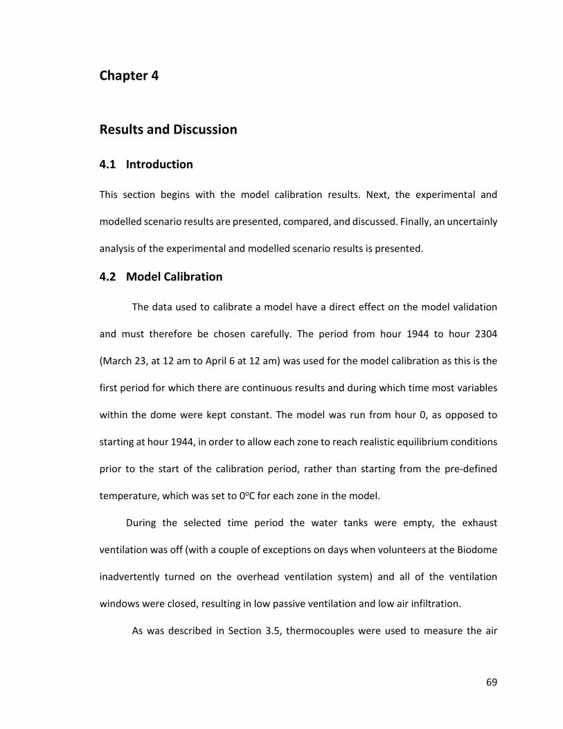
69

Chapter 4

4

Results and Discussion

4.1 Introduction

This section begins with the model calibration results. Next, the experimental and

modelled scenario results are presented, compared, and discussed. Finally, an uncertainly

analysis of the experimental and modelled scenario results is presented.

4.2 Model Calibration

The data used to calibrate a model have a direct effect on the model validation

and must therefore be chosen carefully. The period from hour 1944 to hour 2304

(March 23, at 12 am to April 6 at 12 am) was used for the model calibration as this is the

first period for which there are continuous results and during which time most variables

within the dome were kept constant. The model was run from hour 0, as opposed to

starting at hour 1944, in order to allow each zone to reach realistic equilibrium conditions

prior to the start of the calibration period, rather than starting from the pre-defined

temperature, which was set to 0oC for each zone in the model.

During the selected time period the water tanks were empty, the exhaust

ventilation was off (with a couple of exceptions on days when volunteers at the Biodome

inadvertently turned on the overhead ventilation system) and all of the ventilation

windows were closed, resulting in low passive ventilation and low air infiltration.

As was described in Section 3.5, thermocouples were used to measure the air

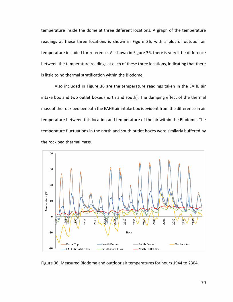
70

temperature inside the dome at three different locations. A graph of the temperature

readings at these three locations is shown in Figure 36, with a plot of outdoor air

temperature included for reference. As shown in Figure 36, there is very little difference

between the temperature readings at each of these three locations, indicating that there

is little to no thermal stratification within the Biodome.

Also included in Figure 36 are the temperature readings taken in the EAHE air

intake box and two outlet boxes (north and south). The damping effect of the thermal

mass of the rock bed beneath the EAHE air intake box is evident from the difference in air

temperature between this location and temperature of the air within the Biodome. The

temperature fluctuations in the north and south outlet boxes were similarly buffered by

the rock bed thermal mass.

Figure 36: Measured Biodome and outdoor air temperatures for hours 1944 to 2304.

71

It was noted that the temperature variation in the south outlet box was much

greater than that of the north outlet box. Upon further investigation a large gap was

discovered in the exterior wall of the south outlet box, next to the door frame, which

allowed a high air infiltration rate into this area, causing unusually high daily temperature

swings. This gap was later repaired with spray-in foam insulation, which reduced the

temperature difference between the two outlet boxes.

For the calibration between the modelled results and the measured results of the

air temperature in the Biodome, an average of the temperature readings at the dome

top, north, and south, will be used in order to account for the slight differences in air

temperature due to stratification.

As shown in Figure 37, the temperature readings taken throughout the EAHE pipes

and in the north and south soil are much more variable than the Biodome air temperature

readings. The most variable EAHE pipe temperature readings were taken in pipe 3. These

large variations can be attributed to the fact that pipe 3 shifted during installation and is

located much closer to the surface of the rock bed than had been planned. As such, it is

subject to larger temperature variations through the rock bed surface.

For the calibration between the modelled results and the measured results, an

average of the temperature readings in the north soil, south soil, 2/3 of pipe 2, and 2/3

of pipe 5 will be used in order to incorporate the effect of the temperature gradient

through the soil.

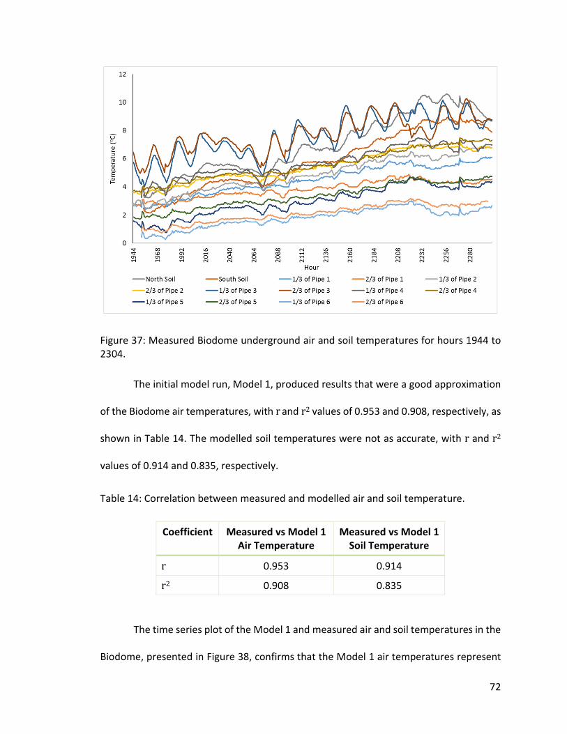
72

Figure 37: Measured Biodome underground air and soil temperatures for hours 1944 to

2304.

The initial model run, Model 1, produced results that were a good approximation

of the Biodome air temperatures, with r and r2 values of 0.953 and 0.908, respectively, as

shown in Table 14. The modelled soil temperatures were not as accurate, with r and r2

values of 0.914 and 0.835, respectively.

Table 14: Correlation between measured and modelled air and soil temperature.

Coefficient Measured vs Model 1

Air Temperature

Measured vs Model 1

Soil Temperature

r 0.953 0.914

r2 0.908 0.835

The time series plot of the Model 1 and measured air and soil temperatures in the

Biodome, presented in Figure 38, confirms that the Model 1 air temperatures represent

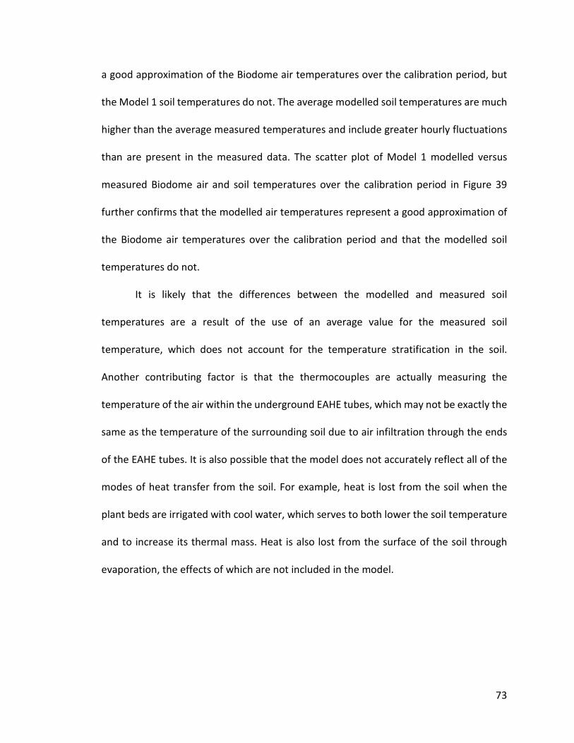
73

a good approximation of the Biodome air temperatures over the calibration period, but

the Model 1 soil temperatures do not. The average modelled soil temperatures are much

higher than the average measured temperatures and include greater hourly fluctuations

than are present in the measured data. The scatter plot of Model 1 modelled versus

measured Biodome air and soil temperatures over the calibration period in Figure 39

further confirms that the modelled air temperatures represent a good approximation of

the Biodome air temperatures over the calibration period and that the modelled soil

temperatures do not.

It is likely that the differences between the modelled and measured soil

temperatures are a result of the use of an average value for the measured soil

temperature, which does not account for the temperature stratification in the soil.

Another contributing factor is that the thermocouples are actually measuring the

temperature of the air within the underground EAHE tubes, which may not be exactly the

same as the temperature of the surrounding soil due to air infiltration through the ends

of the EAHE tubes. It is also possible that the model does not accurately reflect all of the

modes of heat transfer from the soil. For example, heat is lost from the soil when the

plant beds are irrigated with cool water, which serves to both lower the soil temperature

and to increase its thermal mass. Heat is also lost from the surface of the soil through

evaporation, the effects of which are not included in the model.

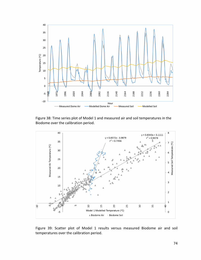
74

Figure 38: Time series plot of Model 1 and measured air and soil temperatures in the

Biodome over the calibration period.

Figure 39: Scatter plot of Model 1 results versus measured Biodome air and soil

temperatures over the calibration period.

75

Measurable or identifiable geometries, materials, and schedules were used in the

model, but the physical characteristics of some materials were not known and were

approximated. These approximated characteristics were used as adjustable parameters

to improve model fit during the model calibration.

The only surface in the Biodome model for which physical characteristics were varied

was that of the soil surface, as this is the main surface whose properties are most

uncertain due to the variable nature of soil, which depend on its composition, moisture

content, etc. The properties of the soil surface that were varied in order to determine

their effect on model fit were solar absorptance and the convective heat transfer

coefficient. Both of these properties and their effect on the model results are described

in the following sections.

4.2.1 Solar Absorptance Calibration

For Model 2, the default solar absorptance values for the front and back surfaces of the

soil were changed to 0.9, which would be appropriate for a near-black body. The r and r2

for the measured versus modelled air and soil temperatures for Model 1 and Model 2 are

shown in Table 15. Although the effects of these changes on the modelled air

temperatures were very small, they resulted in less accurate modelled soil temperature

results than those of Model 1.

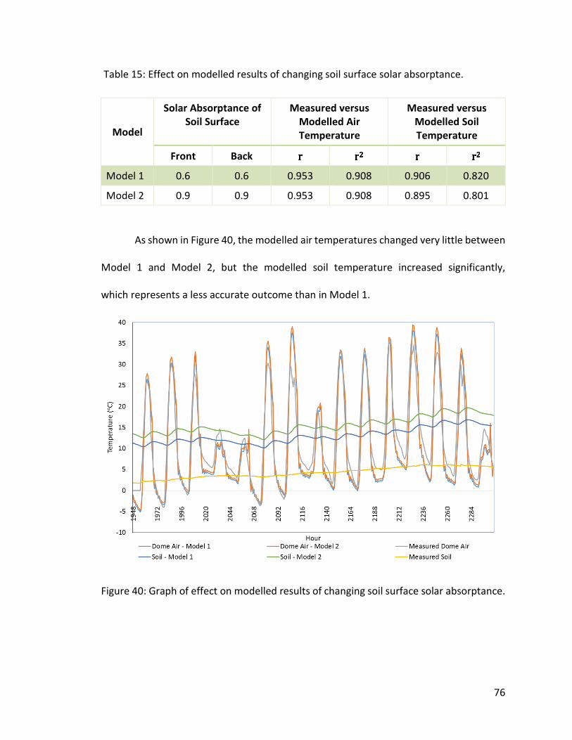
76

Table 15: Effect on modelled results of changing soil surface solar absorptance.

Model

Solar Absorptance of

Soil Surface

Measured versus

Modelled Air

Temperature

Measured versus

Modelled Soil

Temperature

Front Back rrrr rrrr2222 rrrr rrrr2222

Model 1 0.6 0.6 0.953 0.908 0.906 0.820

Model 2 0.9 0.9 0.953 0.908 0.895 0.801

As shown in Figure 40, the modelled air temperatures changed very little between

Model 1 and Model 2, but the modelled soil temperature increased significantly,

which represents a less accurate outcome than in Model 1.

Figure 40: Graph of effect on modelled results of changing soil surface solar absorptance.

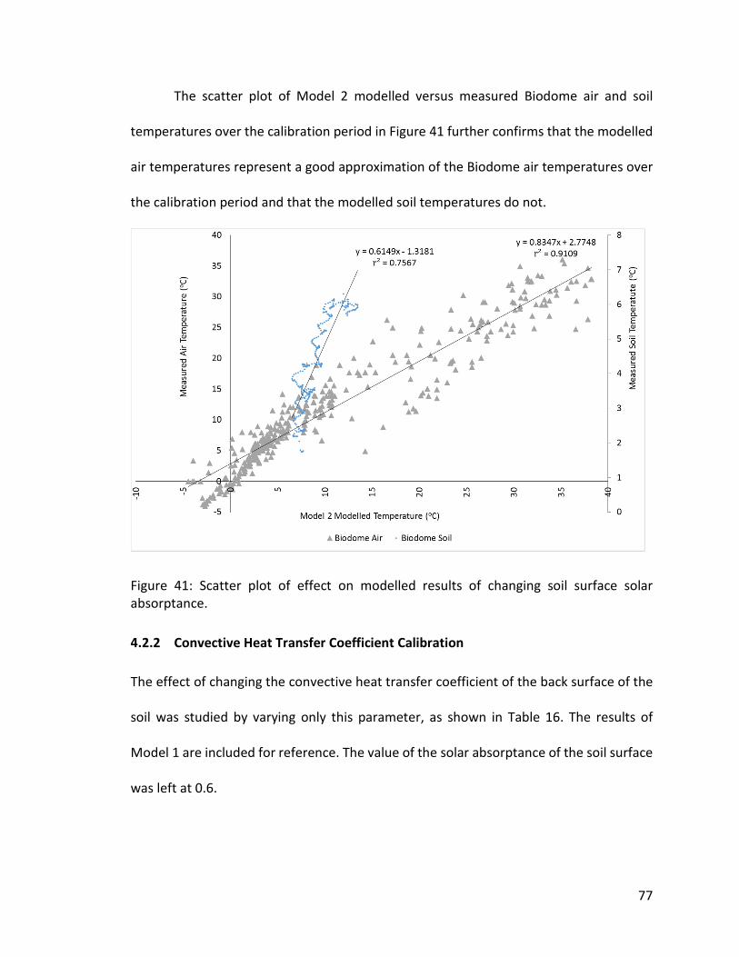
77

The scatter plot of Model 2 modelled versus measured Biodome air and soil

temperatures over the calibration period in Figure 41 further confirms that the modelled

air temperatures represent a good approximation of the Biodome air temperatures over

the calibration period and that the modelled soil temperatures do not.

Figure 41: Scatter plot of effect on modelled results of changing soil surface solar

absorptance.

4.2.2 Convective Heat Transfer Coefficient Calibration

The effect of changing the convective heat transfer coefficient of the back surface of the

soil was studied by varying only this parameter, as shown in Table 16. The results of

Model 1 are included for reference. The value of the solar absorptance of the soil surface

was left at 0.6.

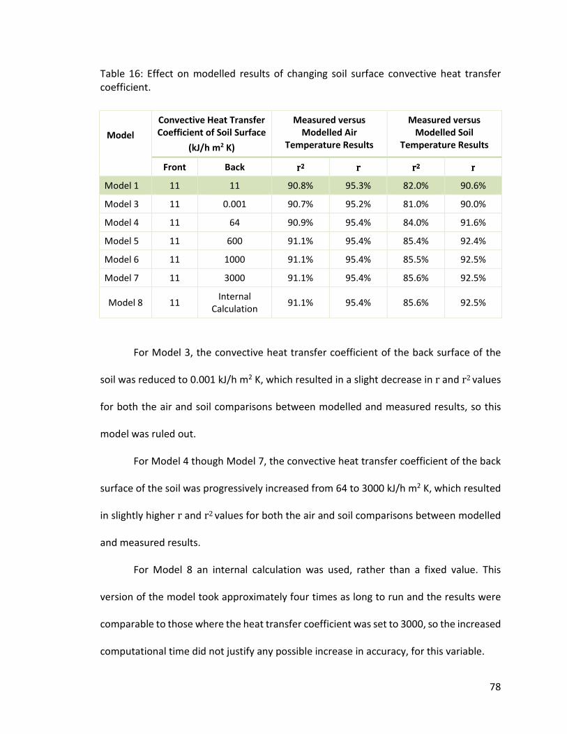
78

Table 16: Effect on modelled results of changing soil surface convective heat transfer

coefficient.

Model

Convective Heat Transfer

Coefficient of Soil Surface

(kJ/h m2 K)

Measured versus

Modelled Air

Temperature Results

Measured versus

Modelled Soil

Temperature Results

Front Back rrrr2222 rrrr rrrr2222 rrrr

Model 1 11 11 90.8% 95.3% 82.0% 90.6%

Model 3 11 0.001 90.7% 95.2% 81.0% 90.0%

Model 4 11 64 90.9% 95.4% 84.0% 91.6%

Model 5 11 600 91.1% 95.4% 85.4% 92.4%

Model 6 11 1000 91.1% 95.4% 85.5% 92.5%

Model 7 11 3000 91.1% 95.4% 85.6% 92.5%

Model 8 11 Internal

Calculation 91.1% 95.4% 85.6% 92.5%

For Model 3, the convective heat transfer coefficient of the back surface of the

soil was reduced to 0.001 kJ/h m2 K, which resulted in a slight decrease in r and r2 values

for both the air and soil comparisons between modelled and measured results, so this

model was ruled out.

For Model 4 though Model 7, the convective heat transfer coefficient of the back

surface of the soil was progressively increased from 64 to 3000 kJ/h m2 K, which resulted

in slightly higher r and r2 values for both the air and soil comparisons between modelled

and measured results.

For Model 8 an internal calculation was used, rather than a fixed value. This

version of the model took approximately four times as long to run and the results were

comparable to those where the heat transfer coefficient was set to 3000, so the increased

computational time did not justify any possible increase in accuracy, for this variable.

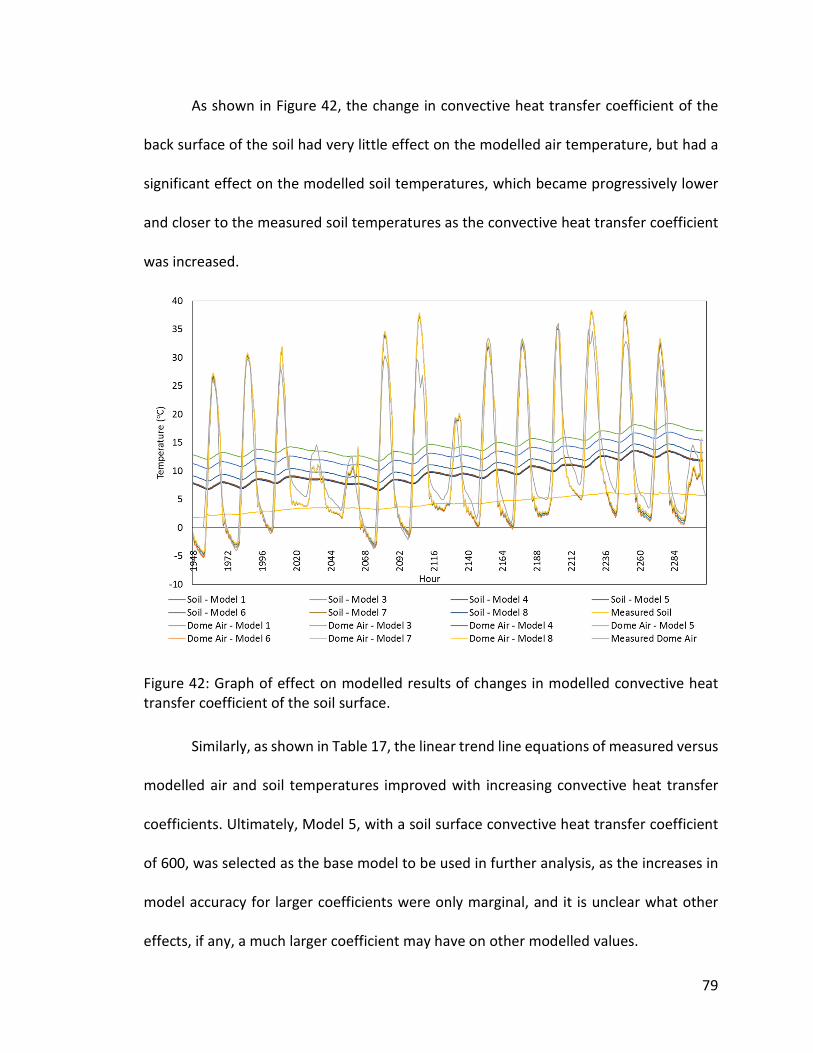
79

As shown in Figure 42, the change in convective heat transfer coefficient of the

back surface of the soil had very little effect on the modelled air temperature, but had a

significant effect on the modelled soil temperatures, which became progressively lower

and closer to the measured soil temperatures as the convective heat transfer coefficient

was increased.

Figure 42: Graph of effect on modelled results of changes in modelled convective heat

transfer coefficient of the soil surface.

Similarly, as shown in Table 17, the linear trend line equations of measured versus

modelled air and soil temperatures improved with increasing convective heat transfer

coefficients. Ultimately, Model 5, with a soil surface convective heat transfer coefficient

of 600, was selected as the base model to be used in further analysis, as the increases in

model accuracy for larger coefficients were only marginal, and it is unclear what other

effects, if any, a much larger coefficient may have on other modelled values.

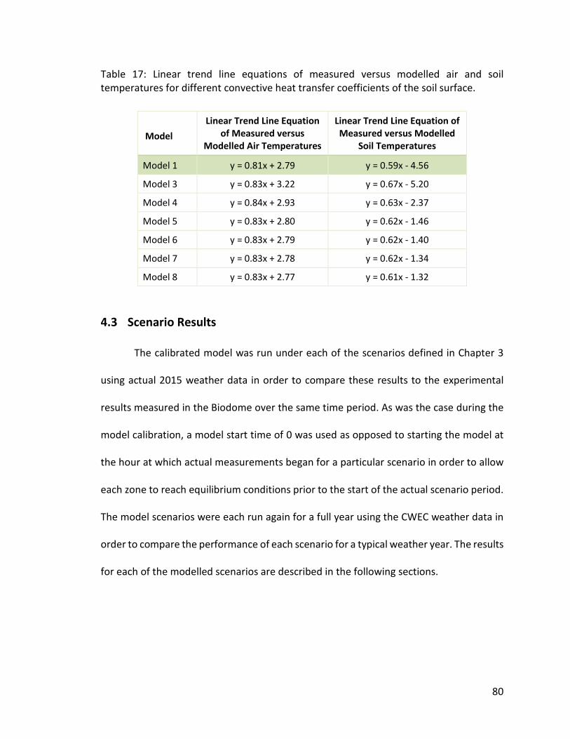
80

Table 17: Linear trend line equations of measured versus modelled air and soil

temperatures for different convective heat transfer coefficients of the soil surface.

Model

Linear Trend Line Equation

of Measured versus

Modelled Air Temperatures

Linear Trend Line Equation of

Measured versus Modelled

Soil Temperatures

Model 1 y = 0.81x + 2.79 y = 0.59x - 4.56

Model 3 y = 0.83x + 3.22 y = 0.67x - 5.20

Model 4 y = 0.84x + 2.93 y = 0.63x - 2.37

Model 5 y = 0.83x + 2.80 y = 0.62x - 1.46

Model 6 y = 0.83x + 2.79 y = 0.62x - 1.40

Model 7 y = 0.83x + 2.78 y = 0.62x - 1.34

Model 8 y = 0.83x + 2.77 y = 0.61x - 1.32

4.3 Scenario Results

The calibrated model was run under each of the scenarios defined in Chapter 3

using actual 2015 weather data in order to compare these results to the experimental

results measured in the Biodome over the same time period. As was the case during the

model calibration, a model start time of 0 was used as opposed to starting the model at

the hour at which actual measurements began for a particular scenario in order to allow

each zone to reach equilibrium conditions prior to the start of the actual scenario period.

The model scenarios were each run again for a full year using the CWEC weather data in

order to compare the performance of each scenario for a typical weather year. The results

for each of the modelled scenarios are described in the following sections.

81

4.3.1 Scenario A

Model Scenario A represents the case where the Biodome is run as a closed system, with

no forced ventilation, no extra thermal mass. Measured results for the period from hour

1951 to 2302 are used as the actual results for this time period. This scenario presents

the same conditions as those used for model calibration, so it also serves the function of

model validation using the calibrated model.

As shown in the time series plot of Scenario A versus measured air and soil

temperatures, in Figure 43, the modelled Scenario A results for Biodome air temperature

match the measured air temperatures well, but the modelled soil temperatures are

consistently higher and show more daily variation than the measured temperatures. The

three visible dips in measured air temperature at hours 2103, 2222, and 2271 were all

caused by the forced overhead ventilation being turned on inadvertently by volunteers

working in the Biodome.

As shown in the scatter plot in Figure 44, the r2 value of the modelled versus

measured air and soil temperatures are 0.91 and 0.88, respectively, which further

indicates good model fit of the air temperature results, but less good fit of the soil

temperature results.

82

Figure 43: Time series plot of Scenario A modelled and measured air and soil temperatures in the Biodome.

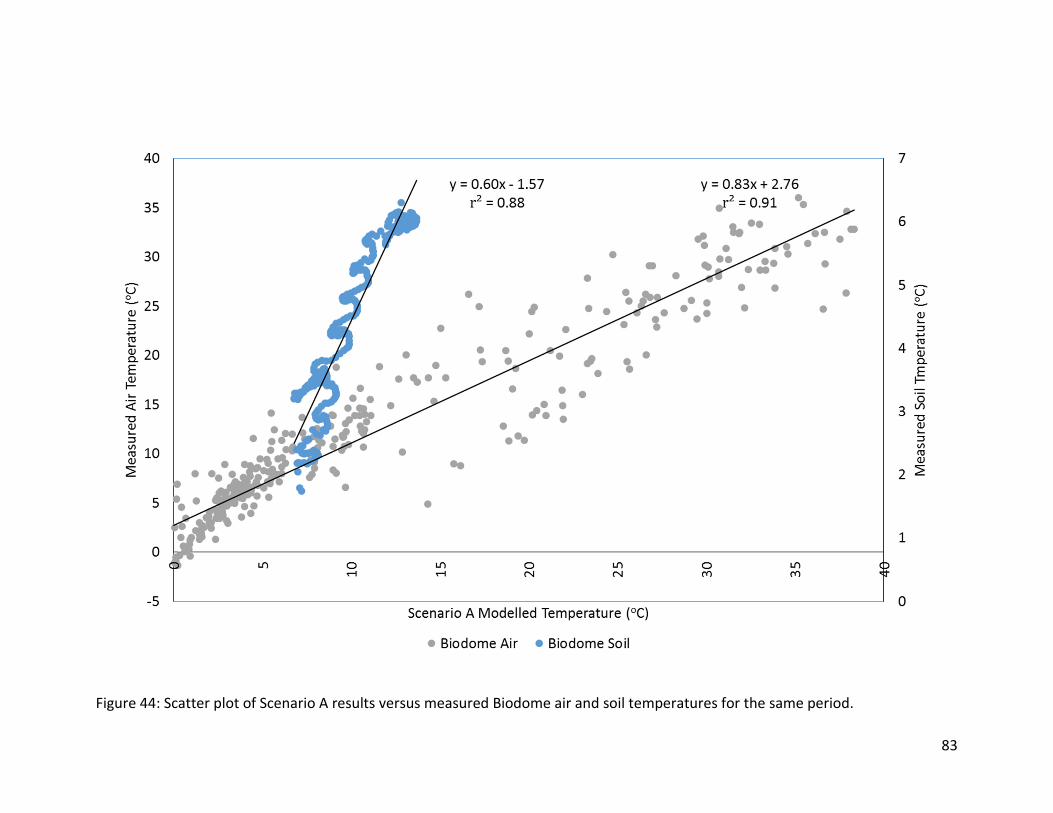
83

Figure 44: Scatter plot of Scenario A results versus measured Biodome air and soil temperatures for the same period.

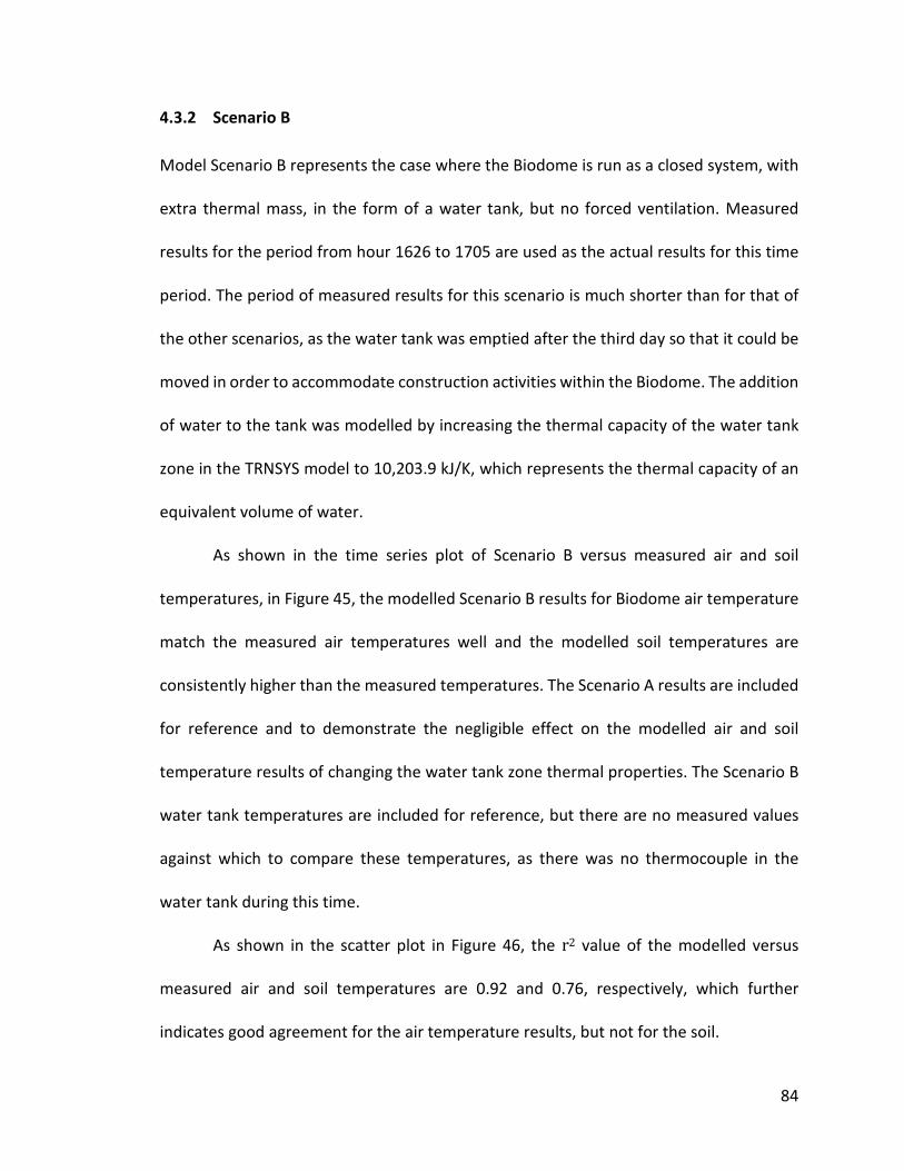
84

4.3.2 Scenario B

Model Scenario B represents the case where the Biodome is run as a closed system, with

extra thermal mass, in the form of a water tank, but no forced ventilation. Measured

results for the period from hour 1626 to 1705 are used as the actual results for this time

period. The period of measured results for this scenario is much shorter than for that of

the other scenarios, as the water tank was emptied after the third day so that it could be

moved in order to accommodate construction activities within the Biodome. The addition

of water to the tank was modelled by increasing the thermal capacity of the water tank

zone in the TRNSYS model to 10,203.9 kJ/K, which represents the thermal capacity of an

equivalent volume of water.

As shown in the time series plot of Scenario B versus measured air and soil

temperatures, in Figure 45, the modelled Scenario B results for Biodome air temperature

match the measured air temperatures well and the modelled soil temperatures are

consistently higher than the measured temperatures. The Scenario A results are included

for reference and to demonstrate the negligible effect on the modelled air and soil

temperature results of changing the water tank zone thermal properties. The Scenario B

water tank temperatures are included for reference, but there are no measured values

against which to compare these temperatures, as there was no thermocouple in the

water tank during this time.


measured air and soil temperatures are 0.92 and 0.76, respectively, which further

indicates good agreement for the air temperature results, but not for the soil.

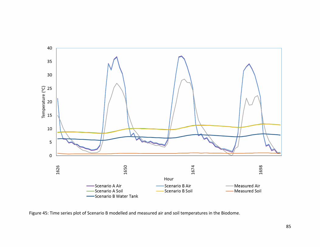
85

Figure 45: Time series plot of Scenario B modelled and measured air and soil temperatures in the Biodome.

86

Figure 46: Scatter plot of Scenario B results versus measured Biodome air and soil temperatures for the same period.

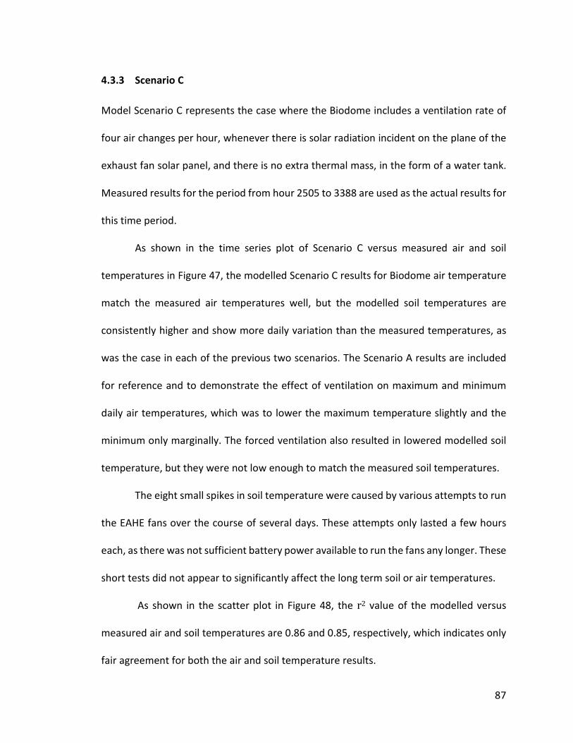
87

4.3.3 Scenario C

Model Scenario C represents the case where the Biodome includes a ventilation rate of

four air changes per hour, whenever there is solar radiation incident on the plane of the

exhaust fan solar panel, and there is no extra thermal mass, in the form of a water tank.

Measured results for the period from hour 2505 to 3388 are used as the actual results for

this time period.

As shown in the time series plot of Scenario C versus measured air and soil

temperatures in Figure 47, the modelled Scenario C results for Biodome air temperature

match the measured air temperatures well, but the modelled soil temperatures are

consistently higher and show more daily variation than the measured temperatures, as

was the case in each of the previous two scenarios. The Scenario A results are included

for reference and to demonstrate the effect of ventilation on maximum and minimum

daily air temperatures, which was to lower the maximum temperature slightly and the

minimum only marginally. The forced ventilation also resulted in lowered modelled soil

temperature, but they were not low enough to match the measured soil temperatures.

The eight small spikes in soil temperature were caused by various attempts to run

the EAHE fans over the course of several days. These attempts only lasted a few hours

each, as there was not sufficient battery power available to run the fans any longer. These

short tests did not appear to significantly affect the long term soil or air temperatures.


measured air and soil temperatures are 0.86 and 0.85, respectively, which indicates only

fair agreement for both the air and soil temperature results.

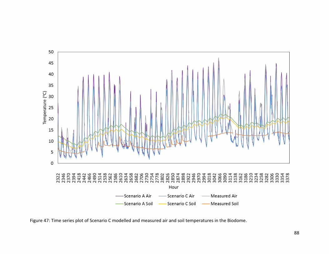
88

Figure 47: Time series plot of Scenario C modelled and measured air and soil temperatures in the Biodome.

89

Figure 48: Scatter plot of Scenario C results versus measured Biodome air and soil temperatures for the same period.

90

4.3.4 Scenario D

Model Scenario D represents the case where the Biodome includes a ventilation rate of


exhaust fan solar panel; there is extra thermal mass, in the form of the water tank

containing 2592 L of water; and there is no shading resulting from the installation of the

solar panels. Measured results for the period from hour 3883 to 4049 are used as the

actual results for this time period.

As shown in the time series plot of Scenario D result versus measured air, water,

and soil temperatures, in Figure 49, the modelled Scenario D results for Biodome air

temperature are consistently lower than the measured results, although their hourly

variation patterns are very similar. Similarly, the Scenario D soil temperatures were once

again slightly higher than the measured soil temperatures. Conversely, the Scenario D

water temperatures were much lower than the measured water temperatures, with

differences of between 13 and 15oC.

The Scenario C results are included for reference and to demonstrate the effect

on the modelled air and soil temperature of changing the water tank zone thermal

properties. Compared to Scenario C, the air temperatures variations are slightly

dampened, but there is no significant difference in soil temperatures.


measured air, water, and soil temperatures are 0.85, 0.80, and 0.91, respectively, which

indicates good agreement for soil temperatures, but not air or water temperatures.

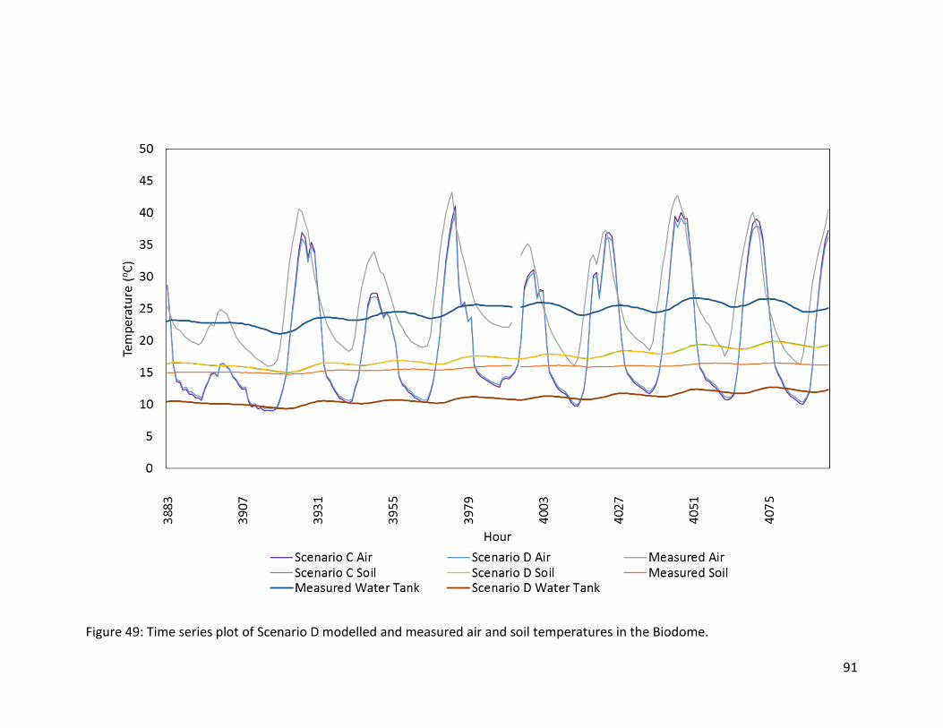
91

Figure 49: Time series plot of Scenario D modelled and measured air and soil temperatures in the Biodome.

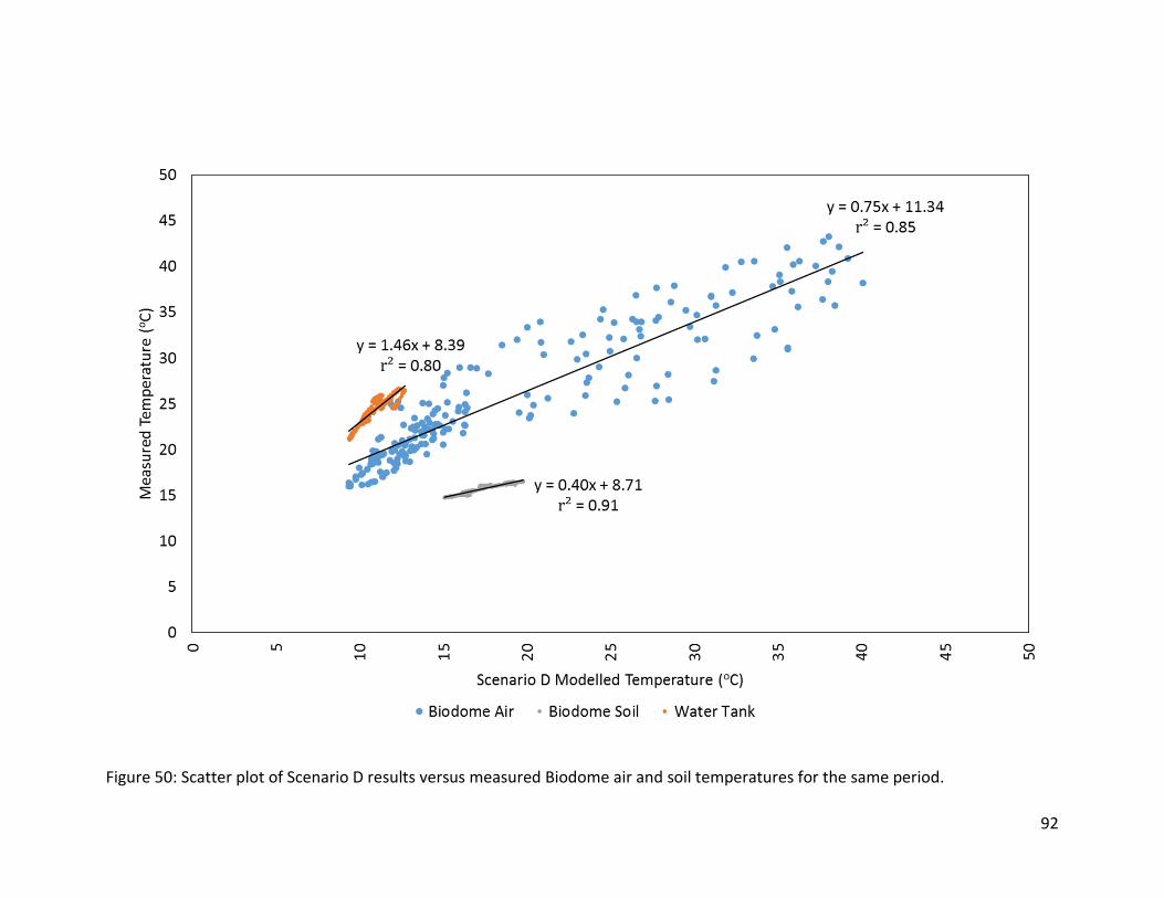
92

Figure 50: Scatter plot of Scenario D results versus measured Biodome air and soil temperatures for the same period.

93

4.3.5 Scenario E

Model Scenario E represents the case where the Biodome includes a ventilation rate of


exhaust fan solar panel; there is extra thermal mass, in the form of the water tanks

containing 2592 L of water; and there is shading resulting from the installation of solar

panels. Measured results for the period from hour 4261 to 4353 are used as the actual

results for this time period.

The time series plot of Scenario E and Scenario D results versus measured air,

water, and soil temperatures, in Figure 51, shows that both Scenario E and Scenario D

produce almost identical model temperatures. This result indicates that there is no effect

on the model of shading two of the Biodome window panels. As there are only about

three days of data under these conditions, it is unclear what the long term effect of the

solar panel shading will be on the Biodome air, water, and soil temperatures.

As shown in the scatter plot Figure 52 in, the r2 value of the modelled versus

measured air, water, and soil temperatures are 0.84, 0.91, and 0.95, respectively.

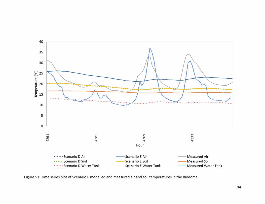
94

Figure 51: Time series plot of Scenario E modelled and measured air and soil temperatures in the Biodome.

95

Figure 52: Scatter plot of Scenario E results versus measured Biodome air and soil temperatures for the same period.

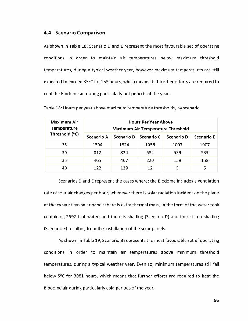
96

4.4 Scenario Comparison

As shown in Table 18, Scenario D and E represent the most favourable set of operating

conditions in order to maintain air temperatures below maximum threshold

temperatures, during a typical weather year, however maximum temperatures are still

expected to exceed 35oC for 158 hours, which means that further efforts are required to

cool the Biodome air during particularly hot periods of the year.

Table 18: Hours per year above maximum temperature thresholds, by scenario

Maximum Air

Temperature

Threshold (oC)

Hours Per Year Above

Maximum Air Temperature Threshold

Scenario A Scenario B Scenario C Scenario D Scenario E

25 1304 1324 1056 1007 1007

30 812 824 584 539 539

35 465 467 220 158 158

40 122 129 12 5 5

Scenarios D and E represent the cases where: the Biodome includes a ventilation

rate of four air changes per hour, whenever there is solar radiation incident on the plane

of the exhaust fan solar panel; there is extra thermal mass, in the form of the water tank

containing 2592 L of water; and there is shading (Scenario D) and there is no shading

(Scenario E) resulting from the installation of the solar panels.

As shown in Table 19, Scenario B represents the most favourable set of operating

conditions in order to maintain air temperatures above minimum threshold

temperatures, during a typical weather year. Even so, minimum temperatures still fall

below 5oC for 3081 hours, which means that further efforts are required to heat the

Biodome air during particularly cold periods of the year.

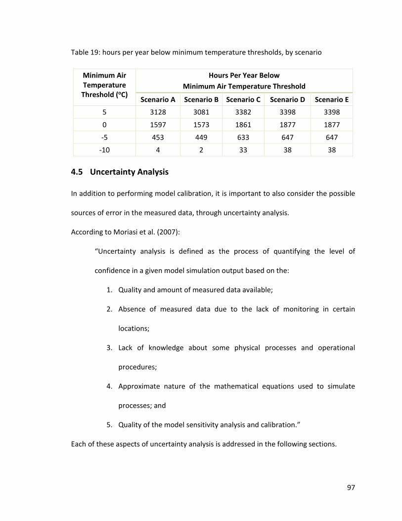
97

Table 19: hours per year below minimum temperature thresholds, by scenario

Minimum Air

Temperature

Threshold (oC)

Hours Per Year Below

Minimum Air Temperature Threshold

Scenario A Scenario B Scenario C Scenario D Scenario E

5 3128 3081 3382 3398 3398

0 1597 1573 1861 1877 1877

-5 453 449 633 647 647

-10 4 2 33 38 38

4.5 Uncertainty Analysis

In addition to performing model calibration, it is important to also consider the possible

sources of error in the measured data, through uncertainty analysis.

According to Moriasi et al. (2007):

“Uncertainty analysis is defined as the process of quantifying the level of

confidence in a given model simulation output based on the:

1. Quality and amount of measured data available;

2. Absence of measured data due to the lack of monitoring in certain

locations;

3. Lack of knowledge about some physical processes and operational

procedures;

4. Approximate nature of the mathematical equations used to simulate

processes; and

5. Quality of the model sensitivity analysis and calibration.”

Each of these aspects of uncertainty analysis is addressed in the following sections.

98

Quality and amount of measured data available

As was stated in Section 3.4.4, the thermocouples used in this project are made from K-

type thermocouple wire that is polyvinyl insulated, 24 AWG stranded, with a special limit

of error (SLE) designation, indicating a reduced error limit, which in this case is the greater

of 1.1oC or 0.4 percent.

The thermocouples were independently calibrated but the results of this

calibration could not be used due to the nature of the ICs that were used to read and

interpret the voltage from the thermocouples, as described in Section 3.4.4. A proper

calibration procedure would have required the use of the completed instrumentation

system, which was not ready until late February 2015 when it became imperative to install

it in the Biodome and begin data collection.

As shown in Table 20, the temperature data resolution of the ICs is 0.25oC and the

temperature gain and offset error is ±1 to ±2oC, guaranteed by design, depending on the

cold-compensation temperature range and the temperature measurement range. As all

of the measurements in this thesis are within the range of -100 to +100oC, the

temperature gain and offset error of the ICs is ±1oC, guaranteed by design. The cold-

junction temperature data resolution is 0.0625oC, with an error range of ±2oC.

Combining the error contributions from both the thermocouple wire and the ICs,

the total error of the temperature measurements in this thesis is ±4.1oC, not including

any errors resulting from thermocouple placement or averaging of results.

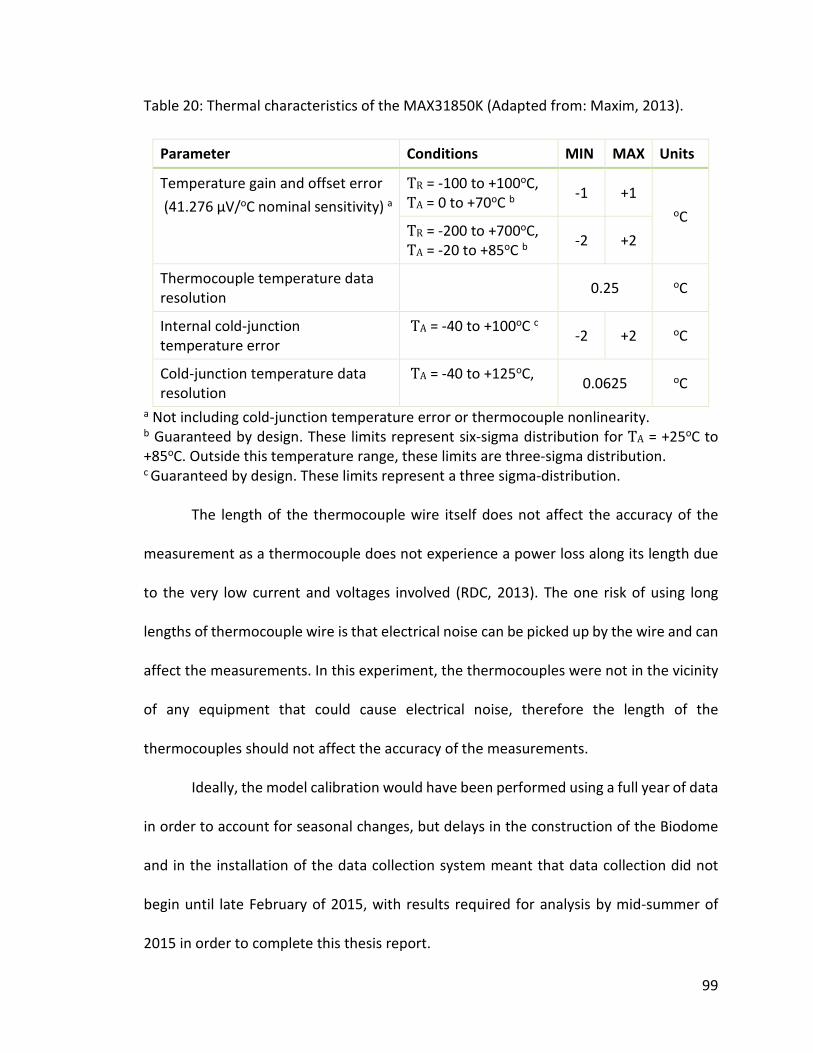
99

Table 20: Thermal characteristics of the MAX31850K (Adapted from: Maxim, 2013).

Parameter Conditions MIN MAX Units

Temperature gain and offset error

(41.276 µV/oC nominal sensitivity) a

TR = -100 to +100oC,

TA = 0 to +70oC b -1 +1

oC TR = -200 to +700oC,

TA = -20 to +85oC b -2 +2

Thermocouple temperature data

resolution

0.25 oC

Internal cold-junction

temperature error

TA = -40 to +100oC c -2 +2 oC

Cold-junction temperature data

resolution

TA = -40 to +125oC, 0.0625 oC

a Not including cold-junction temperature error or thermocouple nonlinearity. b Guaranteed by design. These limits represent six-sigma distribution for TA = +25oC to

+85oC. Outside this temperature range, these limits are three-sigma distribution. c Guaranteed by design. These limits represent a three sigma-distribution.

The length of the thermocouple wire itself does not affect the accuracy of the

measurement as a thermocouple does not experience a power loss along its length due

to the very low current and voltages involved (RDC, 2013). The one risk of using long

lengths of thermocouple wire is that electrical noise can be picked up by the wire and can

affect the measurements. In this experiment, the thermocouples were not in the vicinity

of any equipment that could cause electrical noise, therefore the length of the

thermocouples should not affect the accuracy of the measurements.

Ideally, the model calibration would have been performed using a full year of data

in order to account for seasonal changes, but delays in the construction of the Biodome

and in the installation of the data collection system meant that data collection did not

begin until late February of 2015, with results required for analysis by mid-summer of

2015 in order to complete this thesis report.

100

In addition to the reduced time period for the calibration data, various aspects of

the Biodome operation were not kept consistent throughout the measurement periods,

due to the nature of the operation. As was noted earlier, on a few occasions, volunteers

inadvertently turned on the overhead ventilation, left the front door open, or opened side

vents, which affected the temperature readings during these periods.

Absence of measured data due to the lack of monitoring in certain locations

As the initial intent of this project had been to study the effects of the EAHE on the

temperature in the underground vents and in the plant root zone, a majority of the

thermocouples are located in the EAHE pipes. Given the change in scope of this project

to an assessment of the overall conditions within the Biodome throughout the year, it

would have been useful to have more thermocouples spread out at different levels in the

soil in order to getter a better representation of the soil temperature gradient.

It would have been useful also to have humidity readings of both the air and the

soil, but the humidity sensors were all damaged early on in the process and were not

replaced.

Lack of knowledge about some physical processes and operational procedures

The various mechanisms of heat transfer through the soil beds were not fully understood,

as they were affected by the types of plants being grown, the amount of irrigation

provided, the soil properties, etc.

Nature of the mathematical equations used to simulate processes

As was demonstrated in the literature review, plants have a significant effect on the heat

gain and humidity within a greenhouse (AHSRAE, 2011), yet these effects were not

101

accounted for in the TRNSYS model because it was unclear what kinds of plants would

actually be planted and the starting point for the experiment was bare soil. A more

detailed model of the soil temperature gradients as well as the humidity cycle within the

Biodome may have been appropriate and may have resulted in more accurate results.

A more accurate model of air infiltration may also have been possible if a blower

door test had been done to determine the overall air tightness of the structure.

Finally, although the temperature-versus-voltage relationship of a thermocouple

is not constant, the slope of the K-type thermocouple approaches a constant over the

temperature range from 0 to 1000oC, so a linear equation, such as the one used in this

thesis provides a good approximation (Omega, 2015).

Quality of the model sensitivity analysis and calibration

As was described earlier, calibration of the TRNSYS model was done manually and

consisted of changing the values of the soil surface solar absorptance and convective heat

transfer coefficient while tracking the effect of these changes on the agreement between

modelled and measured results. It is possible that a sensitivity analysis of other model

parameters would also have been appropriate, but the focus was placed on these two

parameters because they were the most uncertain.

4.6 Summary

Five different combinations of ventilation, water tank thermal mass, and solar panel

shading were used to create five Biodome operating scenarios in order to test the effects

of these variables on both the modelled and the experimentally measured results. A

comparison of the results of these modelled scenarios, created using actual 2015 weather

102

data, to experimentally measured results taken over the same time period indicates that

the model is able to accurately represent the effects of ventilation, but it may not be able

to accurately reflect the effects of increased water tank thermal mass or solar panel

shading, as insufficient measured data was available for these comparisons. Future work

will be required to properly characterize these effects and to adjust and recalibrate the

model.

103

Chapter 6

5

Contributions

A considerable amount of time and effort from several volunteers, including the author

of this thesis paper, has resulted in the construction of a successful geodesic dome

greenhouse demonstration project, the Biodome. Although not all of the original

objectives of this thesis project were met, namely the investigation of the use and

effectiveness of an EAHE system, many other useful discoveries have been made and have

positively contributed to the on-going success of the Biodome project.

The main role the author of this thesis played in the Biodome project was to serve

as Energy Lead. In this role, the author’s main contributions to the project included:

• Researching and recommending the type of climate control technology to use

in the Biodome (i.e. EAHE);

• Evaluating and providing advice on many other climate control technologies

and techniques suggested by members of the BPCG association and members

of the local community (i.e. radiant in-floor heating, roof-mounted solar

thermal collectors, floating row covers, thermal screens, electric space heaters,

etc.);

• Using the results of the literature review to design the EAHE, including the

piping layout design, the materials specification, the fan sizing, and the fan

control system design; and

• Providing answers and advice to questions and issues related to energy use and

104

energy requirements, over the course of the project, including battery sizing for

the solar power system, specification of pump size and piping design, and

installation for the aquaponics system.

In addition to the above contributions to the project, the author also provided

support to the Biodome project in the following non-energy areas:

• Providing advice on the procurement of a geodesic dome greenhouse, as

several options were available and had to be compared and evaluated;

• Participating in community consultation sessions;

• Providing advice on selecting a specific location for the Biodome within the

available area at Brewer Park by comparing available options; and

• Providing physical labour and project management at various stages in the

construction process, including during the installation of the EAHE and during

the construction of the aquaponics system.

From a research perspective, the three main areas of contribution resulting from

this thesis are the design of an appropriate data collection and control system, the

collection and analysis of experimental data, and the design of a TRNSYS model that

represents the base case scenario for the Biodome operation. The data collection system

that was designed for this research will continue to log data in the Biodome and will be

used to continue to improve the operations of the Biodome. The specifications for this

systems are explicitly described so that they can be adapted for use in other projects. In

fact, this design is currently being adapted for use in another greenhouse operation in

Ottawa. Once the solar panels are connected to the battery bank, this system will also be

105

used to control the pump in the aquaponics system and the fans in the EAHE system.

As was demonstrated in Chapter 6, the TRNSYS model is able to provide a good

representation of the Biodome air temperature, in the base case scenario. This model can

be used a reference point against which to compare the Biodome air temperature after

future design and operation modifications are made to the Biodome. The main

shortcoming of the Biodome TRNSYS model is that it is not able to provide a good

representation of the Biodome soil or water tank temperatures. Both of these areas of

the model require further work to better reflect the conditions in the Biodome.

106

Chapter 7

6

Conclusions and Future Work

Some conclusions that can be drawn from the results of the full year models that

were created using the CWEC typical weather year data, are that further efforts will be

required to cool the Biodome air during hot periods of the year and energy will be

required to heat the Biodome air during cold periods of the year. In summary, with the

current Biodome design, appropriate growing conditions (as defined in Chapter 2) cannot

be maintained in the Biodome year-round without the use of auxiliary power, in the form

of a supplementary heating source, such as propane, natural gas, or biomass.

Even though year-round operation is not possible with the current Biodome

design, this project is nonetheless valuable for demonstrating the performance of this

non-conventional greenhouse structure and for showcasing different growing methods

and supporting member-driven educational projects, all of which were stated goals of the

project. Furthermore, future work on the use of the EAHE may also extend the growing

season within the Biodome and improve the benefits of this project.

Some improvements that should be made to the existing Biodome structure in

order to optimize its thermal performance include:

Add more ventilation windows. The relatively small windows currently installed

in the Biodome do not provide sufficient air intake area for the forced ventilation system.

Overheating of the Biodome air could be reduced through proper summer ventilation,

which would be facilitated by the installation of larger ventilation windows.

107

Cover the water tanks at night. This practice will help to reduce evaporation from

the water’s surface and will help to lower the indoor air humidity.

Seal air leaks. Some air leaks were identified during the course of this study and

were subsequently repaired. A more thorough inspection of the Biodome should be

performed in order to identify and repair any other major air leaks in order to reduce the

heat loss during the colder months.

Use shade cloth. In the summer, the use of shade cloths over the south side of the

Biodome should be investigated to help reduce the risk of overheating and scorching of

the plants.

Once the solar panels are properly connected and are charging the batteries in the

Biodome, more work should be done to characterize the effects of the EAHE on both soil

and air temperature. Future work in this area could include fan parametric tests whereby

the EAHE fans can be run for different lengths of time to evaluate their effect on air and

soil temperatures and to determine the optimal operating conditions. Different

combinations of fans can also be used to investigate the effect of changes to EAHE air

flow. Replacement humidity sensors should also be added to the data collection system,

as this information would further help to characterize the effects of the EAHE and would

facilitated the calibration of any future models

Other improvements that could be made to the Biodome TRNSYS model in the

future include the addition of an evapotranspiration model to represent the crops, a

humidity and evaporation model to account for the aquaponics system, and a shading

profile to account for shading from the surrounding trees. The soil and water tank

108

portions of the model should also be investigated further, as neither one is able to provide

an accurate representation of actual results.

109

References

Adafruit. (2015). http://www.adafruit.com/

Agriculture Canada. Energy Conserving Urban Greenhouse for Canada: Construction and

Management. 1987.

Alexandra R. Rempel, Alan W. Rempel, Katharine V. Cashman, Ken N. Gates, Catherine J.

Page, Barbara Shaw. Interpretation of passive solar field data with EnergyPlus

models: Un-conventional wisdom from four sunspaces in Eugene, Oregon. Building

and Environment [Journal], Volume 60, February 2013, Pages 158-172, Retrieved

from http://www.sciencedirect.com/science/article/pii/S0360132312003022

American Society of Agricultural and Biological Engineers. 2008. Heating, Ventilating and

Cooling Greenhouses. ANSI/ASAE EP 406.4 Jan 2003 (R2008). St. Joseph, MI.

American Society of Heating, Refrigerating and Air-Conditioning Engineers, Inc. 2011

ASHRAE Handbook - Heating, Ventilating, and Air-Conditioning Applications (SI

Edition). 2011.

Arduino. (2015). What is Arduino? Retrieved from https://www.arduino.cc/

Banff Greenhouse Gardening Society. (2013). Retrieved from

http://banffgreenhouse.com/

Bansal, Vikas, Misra, Rohit, Das Agarwal, Ghansyam, Mathur, Jyotirmay. Transient effect

of soil thermal conductivity and duration of operation on performance of Earth Air

Tunnel Heat Exchanger. Applied Energy [Journal] 103, 2013, Pages 1–11.

Bill C-36: Ontario Local Food Act. (2013) Royal Assent received, November 6, 2013. 40th

Legislature, 2nd session. Ontario: Legislative Assembly of Ontario. Retrieved June

11, 2015.

110

Brewer Park Community Garden. (2013). Retrieved from

http://brewerparkcommunitygarden.weebly.com/

Buckminster Fuller Institute. (2015). About Fuller. Retrieved from https://bfi.org/about-

fuller/big-ideas/geodesic-domes

Buyapi. (2015). Arduino Compatible Precision Real Time Clock Module w/ Temperature

Sensor (DS3231). Retrieved from http://www.buyapi.ca/product/arduino-

compatible-precision-real-time-clock-module-w-temperature-sensor-ds3231/

Campen, J.B., Bot, G.P.A., de Zwart, H.F.. Dehumidification of Greenhouses at Northern

Latitudes. Biosystems Engineering (2003) 86 (4), 487–493

doi:10.1016/j.biosystemseng.2003.08.008

Chandler, Nathan. 2015. How Geodesic Domes Work. Retrieved from

http://science.howstuffworks.com/engineering/structural/geodesic-dome.htm

City of Ottawa, 2009. Community Garden Action Plan Evaluation. Retrieved from

https://app06.ottawa.ca/calendar/ottawa/citycouncil/occ/2009/04-

08/cpsc/01%20-%20ACS2009-COS-RCS-0005%20Gardens.htm

City of Vancouver. (2012). Community gardens growing at record pace across the city.

Retrieved from http://vancouver.ca/news-calendar/community-gardens-growing-

at-record-pace-across-the-city.aspx

Diver, Steve. Aquaponics—Integration of Hydroponics with Aquaculture. 2006. Retrieved

from http://www.backyardaquaponics.com/Travis/aquaponic.pdf

D. N. Moriasi, J. G. Arnold, M. W. Van Liew, R. L. Bingner, R. D. Harmel, T. L. Veith. 2007.

Model evaluation guidelines for systematic quantification of accuracy in watershed

simulations. American Society of Agricultural and Biological Engineers ISSN

0001−235, Vol. 50(3): 885−900.

111

Eden Project. 2015. Architecture at Eden. Retrieved from

http://www.edenproject.com/eden-story/behind-the-scenes/architecture-at-eden

Environment Canada. 2015. 1971 to 2000 Canadian Climate Normals station data.

Retrieved from

http://climate.weather.gc.ca/climate_normals/results_1981_2010_e.html?stnID=

4333&lang=e&StationName=ottawa&SearchType=Contains&stnNameSubmit=go&

dCode=1. Date modified: 2015-02-11

Exner-Pirot, Heather. 2012. Guidelines for Establishing a Northern Greenhouse Project.

International Centre for Northern Governance and Development. 2012.

Fuchs, M., E. Dayan, D. Shmuel and I. Zipori, 1997. Effects of ventilation on the energy

balance of a greenhouse with bare soil. Agricultural and Forest Meteorol., 86 (3-4):

273-282.

Fuller R.J., Meyer C.P. and Sale P.J.M. Validation of a dynamic model for predicting

energy use in greenhouse [Journal] // Journal of Agricultural Engineering. 1987. 38.

pp. 1-14.

Fuller, R.J.. Solar heating systems for recirculating aquaculture. Aquacultural Engineering

36 (2007) 250–260.

GAF. Green Machine Solar-Powered EcoSmart Roof Vent. 2005 Retrieved from

http://www.gaf.ca/Roofing/Residential/Products/Roof_Vents/MasterFlow_Solar_

Powered_Exhaust

Geo-dome. Geodesic dome frequency explained. Retrieved from http://geo-

dome.co.uk/article.asp?uname=domefreq

Ghosal, M.K., Tiwari, G.N., 2006. Modeling and parametric studies for thermal

performance of an earth to air heat exchanger integrated with a greenhouse.

Energy Conversion and Management 47 (13–14), 1779–1798.

112

Goch, Taff. Geodesic Dome Construction Tutorial. Retrieved from

https://3dwarehouse.sketchup.com/model.html?id=81a19157ae1a77fa8f41a8466

c140b06

Google Maps. (2015). Brewer Park Community Garden. [Street map]. Google. Retrieved

from

https://www.google.ca/maps/place/Brewer+Park+Community+Garden/@45.3890

787,-75.6920159

Google Maps. (2015b). Brewer Park Community Garden. [Earth]. Google. Retrieved from

https://www.google.ca/maps/@45.3944733,-

75.7110596,13994m/data=!3m1!1e3

Gupta, Amita, Tiwari, G.N. Computer model and its validation for prediction of storage

effect of water mass in a greenhouse: a transient analysis. Energy Conversion and

Management, Volume 43, Issue 18, December 2002, Pages 2625-2640, ISSN 0196-

8904, http://dx.doi.org/10.1016/S0196-8904(01)00196-0.

(http://www.sciencedirect.com/science/article/pii/S0196890401001960)

Hoes H. and Desmedt J. The GESKAS project, closed greenhouse as energy source and

optimal growing environment. [Journal] // ActaHort.. [s.l.] : ISHS, 2008. - 801.

Hollmuller, Pierre and Lachal, Bernard. TRNSYS compatible moist air hypocaust model.

[Report] Final report / University De Geneve. - [s.l.]: Centre universitaire d'tude

des problemes de l'energie, 1998. - Project number 19507.

Ipsos-Reid. Canadians See Many Benefits of Locally Grown Food. December 1, 2006,

Ipsos-Reid press release. Retrieved from http://www.ipsos-

na.com/news/pressrelease.cfm?id=3298.

113

Johannes F.J. Max, Gerhard Reisinger, Thomas Hofmann, Josef Hinken, Hans-Jürgen

Tantau, Andreas Ulbrich, Susanne Lambrecht, Burkhard von Elsner, Ulrich Schurr.

Glass–film-combination: Opto-physical properties and energy saving potential of a

novel greenhouse glazing system. Energy and Buildings, Volume 50, July 2012,

Pages 298-307, ISSN 0378-7788, Retrieved from

http://dx.doi.org/10.1016/j.enbuild.2012.03.051.

Just Food. Community Gardening Network. 2015. Retrieved from

http://www.justfood.ca/community-gardening-network/

Lamnatou, Chr., Chemisan, D. Solar radiation manipulations and their role in greenhouse

claddings: Fresen lenses, NIR- and UV-blocking materials. 49:135-146. Renewable

and Sustainable Energy Reviews 18 (2013) 271–287.

LBNL, 2013, WINDOW 6.3, Lawrence Berkeley National Laboratory:

https://windows.lbl.gov/software/window/6/

Maxim Integrated. (2013). MAX31850/MAX31851 Cold-Junction Compensated, 1-Wire

Thermocouple-to-Digital Converters. Retrieved from

http://www.adafruit.com/datasheets/MAX31850-MAX31851.pdf

McCullagh, James C. The Solar Greenhouse Book. Rodale Press, Inc. 1978.

Missouri Botanical Garden. (2015). Climatron: Geodesic Dome Conservatory. Retrieved

from http://www.missouribotanicalgarden.org/gardens-gardening/our-

garden/gardens-conservatories/conservatories/climatron.aspx

Moretti, Elisa, Zinzi, Michele, Belloni, Elisa. Polycarbonate panels for buildings:

Experimental investigation of thermal and optical performance. Energy and

Buildings 70 (2014) 23-35.

114

N. Katsoulas, T. Bartzanas, T. Boulard, M. Mermier, C. Kittas. Effect of Vent Openings and

Insect Screens on Greenhouse Ventilation. Biosystems Engineering (2006) 93 (4),

427–436 doi:10.1016/j.biosystemseng.2005.01.001 SE—Structures and

Environment

Numerical Logics. 1999. Canadian Weather for Energy Calculations, Users Manual and

CD-ROM. Downsview, Ontario: Environment Canada.

Omega. (2015). Reference Temperatures. Retrieved from

http://www.omega.com/temperature/z/pdf/z021-032.pdf

Open Source Initiative. (2015). The Open Source Definition (Annotated). Retrieved from

http://opensource.org/osd-annotated

Pérez Parra, J., Baeza, E., López, J.C., Pérez, C., Montero, J.I. and Antón, A. (2003). Effect

of vent types and insect screens on ventilation of "parral" greenhouses. Acta

Hortic. 614, 393-400. Retrieved from

http://dx.doi.org/10.17660/ActaHortic.2003.614.59"

Polygal. 2011. Polygal Polycarbonate Multiwall Sheets Technical Specifications.

Retrieved from http://polygal-northamerica.com/pdf/Polygal-Technical-Guide.pdf

Prime Minister of Canada Stephen Harper. PM announces measures to promote

Northern agriculture. Retrieved from http://pm.gc.ca/eng/news/2014/08/22/pm-

announces-measures-promote-northern-agriculture

Provenzano Jr, Anthony J., Joseph G. Winfield. Performance of a Recirculating Fish

Production System Stocked with Tilapia Hybrids. Aquacultural Engineering 6.1

(1987): 15-26. Web. 14 July 2015.

115

RDC Control. Introduction to Thermocouples. 2013. Retrieved from

http://rdccontrol.com/thermocouples/thermocouples-101/introduction-to-

thermocouples/is-there-a-maximum-length-for-thermocouples-and-

thermocouple-wiring/

Reichel, Justina. Vancouver Community Gardens a Growing Trend. 2012. Retrieved from

http://www.theepochtimes.com/n2/canada/vancouver-community-gardens-a-

growing-trend-251691.html.

Rubel, F., and M. Kottek. 2010. Observed and projected climate shifts 1901-2100

depicted by world maps of the Köppen-Geiger climate classification. Meteorol. Z.,

19, 135-141. DOI: 10.1127/0941-2948/2010/0430.

Santamouris, M., Balaras, C.A., Dascalaki, E., Vallindras, M., 1994. Passive solar

agricultural greenhouses: a worldwide classification and evaluation of

technologies and systems used for heating purposes. Solar Energy 53 (5), 411–426.

Sethi V.P. and S.K. Sharma. (2007). Thermal modeling of a greenhouse integrated to an

aquifer coupled cavity flow heat exchanger system [Journal] Solar Energy 81. pp.

723-741.

Sethi, V.P. On the selection of shape and orientation of a greenhouse: Thermal modeling

and experimental validation. [Journal] Solar Energy 83 (2009) 21–38.

Sethi, V.P., Sharma, S.K.. Survey and evaluation of cooling technologies for worldwide

agricultural greenhouse applications. [Journal] Solar Energy 81 (2007) 1447-1459

Sethi, V.P., Sharma, S.K.. Survey and evaluation of heating technologies for worldwide

agricultural greenhouse applications. [Journal] Solar Energy 82 (2008) 832–859

Snedecor, G.W. and Cochran, W.G. (1982) Statistical Methods. 7th Edition, Iowa State

University Press, Towa, 511.

116

Solar Energy Laboratory, University of Wisconsin–Madison. (2012). TRNSYS: A Transient

Systems Simulation Tool. Accessible online at http://sel.me. wisc.edu/trnsys/.

Statistics Canada. Table 001-0047: Estimates of specialized greenhouse operations,

greenhouse area, and months of operation, annual. CANSIM (database). (accessed:

2015-07-05)

Vadiee, Amir. (2013). Energy management in large scale solar buildings: The closed

greenhouse concept. (Doctoral Thesis) KTH School of Industrial Engineering and

Management, Department of Energy Technology Division of Heat and Power

Technology, Stockholm, Sweden.

Willits D.H., Chandra P. and Peet M.M. Modelling solar energy storage system for

greenhouse [Journal] // Journal of Agricultural Engineering. 1985. 32. pp. 73-79.

Retrieved from

http://www.sciencedirect.com/science/article/pii/0021863485901209

Wong, B., McClung, L., Snijders, A., McClenahan, D., Thornton, J., 2011. The Application

of Aquifer Thermal Energy Storage in the Canadian Greenhouse Industry. [Journal]

Acta Hortic. 893, 437-444. Retrieved from

http://dx.doi.org/10.17660/ActaHortic.2011.893.42

Zhu, S., Deltour, J., Wang, S.. Modeling the thermal characteristics of greenhouse pond

systems. [Journal] Aquacultural Engineering 18 (1998) 201–217.

117

Appendix A: TRNSYS Input File

TRNSYS - the TRaNsient SYstem Simulation program

The Solar Energy Lab at the University of Wisconsin - Madison, USA

Le Centre Scientifique et Technique du Batiment, Sophia Antipolis, France

Transsolar Energietechnik GmBH, Stuttgart, Germany

Thermal Energy System Specialists, LLC, Madison Wisconsin, USA

Release 17.01.0028

*** Notice at time : 0.000000

Generated by Unit : Not applicable or not available

Generated by Type : Not applicable or not available

Message : The TRNSYS Executable (TRNExe.exe) and main DLL (TRNDll.dll) are

located in "C:\Trnsys17\Exe"

*** Pre-Processing the TRNSYS EQUATIONs and CONSTANTs to check for fatal errors.

*** Pre-Processing of EQUATIONs and CONSTANTs completed with no fatal errors found.

*** Evaluating the EQUATIONs and CONSTANTs to determine their initial values.

*** Finished evaluating the EQUATIONs and CONSTANTs and ready to begin processing

the remainder of the TRNSYS input file.

VERSION 17

************************************************************************

*******

*** TRNSYS input file (deck) generated by TrnsysStudio

*** on Sunday, October 25, 2015 at 21:36

*** from TrnsysStudio project:

C:\Users\pclau_000\Dropbox\Thesis\TRNSYS\June_12\July_28_A.tpf

***

*** If you edit this file, use the File/Import TRNSYS Input File function in

*** TrnsysStudio to update the project.

***

*** If you have problems, questions or suggestions please contact your local

*** TRNSYS distributor or mailto:[email protected]

***

************************************************************************

*******

************************************************************************

118

*******

*** Units

************************************************************************

*******

************************************************************************

*******

*** Control cards

************************************************************************

*******

* START, STOP and STEP

CONSTANTS 3

START=0

STOP=8760

STEP=1

! Start time End time Time step

SIMULATION 0.0000000000000000E+00 8.7600000000000000E+03

1.0000000000000000E+00

! Integration Convergence

TOLERANCES 1.0000000000000002E-03 1.0000000000000002E-03

! Max iterations Max warnings Trace limit

LIMITS 30 30 31

! TRNSYS numerical integration solver method

DFQ 1

! TRNSYS output file width, number of characters

WIDTH 72

! NOLIST statement

LIST

! MAP statement

! Solver statement Minimum relaxation factor Maximum relaxation factor

SOLVER 0

1.000000000000000

1.000000000000000

! Nan DEBUG statement

NAN_CHECK 0

! Overwrite DEBUG statement

119

OVERWRITE_CHECK 0

! disable time report

TIME_REPORT 0

! EQUATION SOLVER statement

EQUATION SOLVING METHOD 0

* User defined CONSTANTS

* EQUATIONS "Wizard settings"

*

EQUATIONS 5

!Rotation angle for building used for adapting azimuth angles

TURN = 0

! Close blinds - radiation on facade in [W/m2 * 3.6]=[kJ/hr]

SHADE_CLOSE = 140 * 3.6

! Open blinds - radiation on facade in [W/m2 * 3.6]=[kJ/hr]

SHADE_OPEN = 120 * 3.6

! Maximum opaque fraction of internal shading device

MAX_ISHADE = 0/100

! Maximum opaque fraction of external shading device

MAX_ESHADE = 0/100

*$UNIT_NAME Wizard settings

*$LAYER Main

*$POSITION 73 180

*------------------------------------------------------------------------------

* EQUATIONS "AzimuthAngles"

*

EQUATIONS 92

! azimuth angle of orientation

AA_H_0_0 = 0 + TURN


AA_S_0_50 = 0 + TURN


AA_S_0_25 = 0 + TURN


AA_S_0_10 = 0 + TURN


AA_S_0_65 = 0 + TURN


AA_S_5_90 = 5 + TURN


AA_S_10_70 = 10 + TURN

120


AA_S_10_90 = 10 + TURN


AA_S_15_45 = 15 + TURN


AA_S_20_30 = 20 + TURN


AA_S_25_55 = 25 + TURN


AA_S_25_65 = 25 + TURN


AA_S_35_75 = 35 + TURN


AA_S_35_90 = 35 + TURN


AA_W_45_55 = 45 + TURN


AA_W_50_30 = 50 + TURN


AA_W_50_65 = 50 + TURN


AA_W_55_45 = 55 + TURN


AA_W_60_75 = 60 + TURN


AA_W_60_90 = 60 + TURN


AA_W_70_50 = 70 + TURN


AA_W_70_10 = 70 + TURN


AA_W_70_25 = 70 + TURN


AA_W_70_65 = 70 + TURN


AA_W_85_90 = 85 + TURN


AA_W_85_75 = 85 + TURN


AA_W_90_45 = 90 + TURN


AA_W_95_30 = 95 + TURN


AA_W_95_70 = 95 + TURN

121


AA_W_100_55 = 100 + TURN


AA_W_110_75 = 110 + TURN


AA_W_110_90 = 110 + TURN


AA_W_115_55 = 115 + TURN


AA_W_120_30 = 120 + TURN


AA_W_120_70 = 120 + TURN


AA_W_125_45 = 125 + TURN


AA_W_130_75 = 130 + TURN


AA_N_135_90 = 135 + TURN


AA_N_145_50 = 145 + TURN


AA_N_145_25 = 145 + TURN


AA_N_145_10 = 145 + TURN


AA_N_145_65 = 145 + TURN


AA_N_155_75 = 155 + TURN


AA_N_155_90 = 155 + TURN


AA_N_160_45 = 160 + TURN


AA_N_160_90 = 160 + TURN


AA_N_165_30 = 165 + TURN


AA_N_165_70 = 165 + TURN


AA_N_170_55 = 170 + TURN


AA_N_175_90 = 175 + TURN


AA_N_180_75 = 180 + TURN

122


AA_N_180_90 = 180 + TURN


AA_N_190_55 = 190 + TURN


AA_N_195_30 = 195 + TURN


AA_N_195_70 = 195 + TURN


AA_N_200_45 = 200 + TURN


AA_N_205_75 = 205 + TURN


AA_N_205_90 = 205 + TURN


AA_N_215_50 = 215 + TURN


AA_N_215_25 = 215 + TURN


AA_N_215_10 = 215 + TURN


AA_N_215_65 = 215 + TURN


AA_E_230_75 = 230 + TURN


AA_E_230_90 = 230 + TURN


AA_E_235_45 = 235 + TURN


AA_E_240_30 = 240 + TURN


AA_E_250_65 = 250 + TURN


AA_E_250_90 = 250 + TURN


AA_E_265_30 = 265 + TURN


AA_E_270_45 = 270 + TURN


AA_E_275_75 = 275 + TURN


AA_E_275_90 = 275 + TURN


AA_E_290_10 = 290 + TURN

123


AA_E_290_25 = 290 + TURN


AA_E_290_50 = 290 + TURN


AA_E_290_65 = 290 + TURN


AA_E_300_75 = 300 + TURN


AA_E_300_90 = 300 + TURN


AA_E_305_45 = 305 + TURN


AA_E_310_30 = 310 + TURN


AA_E_310_65 = 310 + TURN


AA_S_315_55 = 315 + TURN


AA_S_325_75 = 325 + TURN


AA_S_325_90 = 325 + TURN


AA_S_330_90 = 330 + TURN


AA_S_335_55 = 335 + TURN


AA_S_335_65 = 335 + TURN


AA_S_340_30 = 340 + TURN


AA_S_345_45 = 345 + TURN


AA_S_350_70 = 350 + TURN


AA_S_350_90 = 350 + TURN

! solar azimuth corrected by building rotation - Input for Type 56 sun position for SHM

and ISM

AAZM_TYPE56 = AAZM - (TURN)

*$UNIT_NAME AzimuthAngles

*$LAYER Main

*$POSITION 73 63

*------------------------------------------------------------------------------

* EQUATIONS "Radiation"

124

*

EQUATIONS 276

AZEN = [15,16]

AAZM = [15,17]

IT_H_0_0 = [15,24]

IB_H_0_0 = [15,49]

AI_H_0_0 = [15,149]

IT_S_0_50 = [15,25]

IB_S_0_50 = [15,50]

AI_S_0_50 = [15,150]

IT_S_0_25 = [15,26]

IB_S_0_25 = [15,51]

AI_S_0_25 = [15,151]

IT_S_0_10 = [15,27]

IB_S_0_10 = [15,52]

AI_S_0_10 = [15,152]

IT_S_0_65 = [15,28]

IB_S_0_65 = [15,53]

AI_S_0_65 = [15,153]

IT_S_5_90 = [15,29]

IB_S_5_90 = [15,54]

AI_S_5_90 = [15,154]

IT_S_10_70 = [15,30]

IB_S_10_70 = [15,55]

AI_S_10_70 = [15,155]

IT_S_10_90 = [15,31]

IB_S_10_90 = [15,56]

AI_S_10_90 = [15,156]

IT_S_15_45 = [15,32]

IB_S_15_45 = [15,57]

AI_S_15_45 = [15,157]

IT_S_20_30 = [15,33]

IB_S_20_30 = [15,58]

AI_S_20_30 = [15,158]

IT_S_25_55 = [15,34]

IB_S_25_55 = [15,59]

AI_S_25_55 = [15,159]

IT_S_25_65 = [15,35]

IB_S_25_65 = [15,60]

AI_S_25_65 = [15,160]

IT_S_35_75 = [15,36]

IB_S_35_75 = [15,61]

AI_S_35_75 = [15,161]

125

IT_S_35_90 = [15,37]

IB_S_35_90 = [15,62]

AI_S_35_90 = [15,162]

IT_W_45_55 = [15,38]

IB_W_45_55 = [15,63]

AI_W_45_55 = [15,163]

IT_W_50_30 = [15,39]

IB_W_50_30 = [15,64]

AI_W_50_30 = [15,164]

IT_W_50_65 = [15,40]

IB_W_50_65 = [15,65]

AI_W_50_65 = [15,165]

IT_W_55_45 = [15,41]

IB_W_55_45 = [15,66]

AI_W_55_45 = [15,166]

IT_W_60_75 = [15,42]

IB_W_60_75 = [15,67]

AI_W_60_75 = [15,167]

IT_W_60_90 = [15,43]

IB_W_60_90 = [15,68]

AI_W_60_90 = [15,168]

IT_W_70_50 = [15,44]

IB_W_70_50 = [15,69]

AI_W_70_50 = [15,169]

IT_W_70_10 = [15,45]

IB_W_70_10 = [15,70]

AI_W_70_10 = [15,170]

IT_W_70_25 = [15,46]

IB_W_70_25 = [15,71]

AI_W_70_25 = [15,171]

IT_W_70_65 = [15,47]

IB_W_70_65 = [15,72]

AI_W_70_65 = [15,172]

IT_W_85_90 = [15,48]

IB_W_85_90 = [15,73]

AI_W_85_90 = [15,173]

IT_W_85_75 = [15,49]

IB_W_85_75 = [15,74]

AI_W_85_75 = [15,174]

IT_W_90_45 = [15,50]

IB_W_90_45 = [15,75]

AI_W_90_45 = [15,175]

IT_W_95_30 = [15,51]

IB_W_95_30 = [15,76]

126

AI_W_95_30 = [15,176]

IT_W_95_70 = [15,52]

IB_W_95_70 = [15,77]

AI_W_95_70 = [15,177]

IT_W_100_55 = [15,53]

IB_W_100_55 = [15,78]

AI_W_100_55 = [15,178]

IT_W_110_75 = [15,54]

IB_W_110_75 = [15,79]

AI_W_110_75 = [15,179]

IT_W_110_90 = [15,55]

IB_W_110_90 = [15,80]

AI_W_110_90 = [15,180]

IT_W_115_55 = [15,56]

IB_W_115_55 = [15,81]

AI_W_115_55 = [15,181]

IT_W_120_30 = [15,57]

IB_W_120_30 = [15,82]

AI_W_120_30 = [15,182]

IT_W_120_70 = [15,58]

IB_W_120_70 = [15,83]

AI_W_120_70 = [15,183]

IT_W_125_45 = [15,59]

IB_W_125_45 = [15,84]

AI_W_125_45 = [15,184]

IT_W_130_75 = [15,60]

IB_W_130_75 = [15,85]

AI_W_130_75 = [15,185]

IT_N_135_90 = [15,61]

IB_N_135_90 = [15,86]

AI_N_135_90 = [15,186]

IT_N_145_50 = [15,62]

IB_N_145_50 = [15,87]

AI_N_145_50 = [15,187]

IT_N_145_25 = [15,63]

IB_N_145_25 = [15,88]

AI_N_145_25 = [15,188]

IT_N_145_10 = [15,64]

IB_N_145_10 = [15,89]

AI_N_145_10 = [15,189]

IT_N_145_65 = [15,65]

IB_N_145_65 = [15,90]

AI_N_145_65 = [15,190]

IT_N_155_75 = [15,66]

127

IB_N_155_75 = [15,91]

AI_N_155_75 = [15,191]

IT_N_155_90 = [15,67]

IB_N_155_90 = [15,92]

AI_N_155_90 = [15,192]

IT_N_160_45 = [15,68]

IB_N_160_45 = [15,93]

AI_N_160_45 = [15,193]

IT_N_160_90 = [15,69]

IB_N_160_90 = [15,94]

AI_N_160_90 = [15,194]

IT_N_165_30 = [15,70]

IB_N_165_30 = [15,95]

AI_N_165_30 = [15,195]

IT_N_165_70 = [15,72]

IB_N_165_70 = [15,97]

AI_N_165_70 = [15,197]

IT_N_170_55 = [15,73]

IB_N_170_55 = [15,98]

AI_N_170_55 = [15,198]

IT_N_175_90 = [15,74]

IB_N_175_90 = [15,99]

AI_N_175_90 = [15,199]

IT_N_180_75 = [15,75]

IB_N_180_75 = [15,100]

AI_N_180_75 = [15,200]

IT_N_180_90 = [15,76]

IB_N_180_90 = [15,101]

AI_N_180_90 = [15,201]

IT_N_190_55 = [15,77]

IB_N_190_55 = [15,102]

AI_N_190_55 = [15,202]

IT_N_195_30 = [15,78]

IB_N_195_30 = [15,103]

AI_N_195_30 = [15,203]

IT_N_195_70 = [15,79]

IB_N_195_70 = [15,104]

AI_N_195_70 = [15,204]

IT_N_200_45 = [15,80]

IB_N_200_45 = [15,105]

AI_N_200_45 = [15,205]

IT_N_205_75 = [15,81]

IB_N_205_75 = [15,106]

AI_N_205_75 = [15,206]

128

IT_N_205_90 = [15,82]

IB_N_205_90 = [15,107]

AI_N_205_90 = [15,207]

IT_N_215_50 = [15,83]

IB_N_215_50 = [15,108]

AI_N_215_50 = [15,208]

IT_N_215_25 = [15,84]

IB_N_215_25 = [15,109]

AI_N_215_25 = [15,209]

IT_N_215_10 = [15,85]

IB_N_215_10 = [15,110]

AI_N_215_10 = [15,210]

IT_N_215_65 = [15,86]

IB_N_215_65 = [15,111]

AI_N_215_65 = [15,211]

IT_E_230_75 = [15,87]

IB_E_230_75 = [15,112]

AI_E_230_75 = [15,212]

IT_E_230_90 = [15,88]

IB_E_230_90 = [15,113]

AI_E_230_90 = [15,213]

IT_E_235_45 = [15,89]

IB_E_235_45 = [15,114]

AI_E_235_45 = [15,214]

IT_E_240_30 = [15,90]

IB_E_240_30 = [15,115]

AI_E_240_30 = [15,215]

IT_E_250_65 = [15,91]

IB_E_250_65 = [15,116]

AI_E_250_65 = [15,216]

IT_E_250_90 = [15,92]

IB_E_250_90 = [15,117]

AI_E_250_90 = [15,217]

IT_E_265_30 = [15,93]

IB_E_265_30 = [15,118]

AI_E_265_30 = [15,218]

IT_E_270_45 = [15,94]

IB_E_270_45 = [15,119]

AI_E_270_45 = [15,219]

IT_E_275_75 = [15,95]

IB_E_275_75 = [15,120]

AI_E_275_75 = [15,220]

IT_E_275_90 = [15,96]

IB_E_275_90 = [15,121]

129

AI_E_275_90 = [15,221]

IT_E_290_10 = [15,97]

IB_E_290_10 = [15,122]

AI_E_290_10 = [15,222]

IT_E_290_25 = [15,98]

IB_E_290_25 = [15,123]

AI_E_290_25 = [15,223]

IT_E_290_50 = [15,99]

IB_E_290_50 = [15,124]

AI_E_290_50 = [15,224]

IT_E_290_65 = [15,100]

IB_E_290_65 = [15,125]

AI_E_290_65 = [15,225]

IT_E_300_75 = [15,101]

IB_E_300_75 = [15,126]

AI_E_300_75 = [15,226]

IT_E_300_90 = [15,102]

IB_E_300_90 = [15,127]

AI_E_300_90 = [15,227]

IT_E_305_45 = [15,103]

IB_E_305_45 = [15,128]

AI_E_305_45 = [15,228]

IT_E_310_30 = [15,104]

IB_E_310_30 = [15,129]

AI_E_310_30 = [15,229]

IT_E_310_65 = [15,105]

IB_E_310_65 = [15,130]

AI_E_310_65 = [15,230]

IT_S_315_55 = [15,106]

IB_S_315_55 = [15,131]

AI_S_315_55 = [15,231]

IT_S_325_75 = [15,107]

IB_S_325_75 = [15,132]

AI_S_325_75 = [15,232]

IT_S_325_90 = [15,108]

IB_S_325_90 = [15,133]

AI_S_325_90 = [15,233]

IT_S_330_90 = [15,109]

IB_S_330_90 = [15,134]

AI_S_330_90 = [15,234]

IT_S_335_55 = [15,110]

IB_S_335_55 = [15,135]

AI_S_335_55 = [15,235]

IT_S_335_65 = [15,111]

130

IB_S_335_65 = [15,136]

AI_S_335_65 = [15,236]

IT_S_340_30 = [15,112]

IB_S_340_30 = [15,137]

AI_S_340_30 = [15,237]

IT_S_345_45 = [15,113]

IB_S_345_45 = [15,138]

AI_S_345_45 = [15,238]

IT_S_350_70 = [15,114]

IB_S_350_70 = [15,139]

AI_S_350_70 = [15,239]

IT_S_350_90 = [15,115]

IB_S_350_90 = [15,140]

AI_S_350_90 = [15,240]

SOLAR_PANEL = [15,25]/max(1, [15,25])

*$UNIT_NAME Radiation

*$LAYER Main

*$POSITION 196 180

*------------------------------------------------------------------------------

* Model "Weather data" (Type 15)

*

UNIT 15 TYPE 15 data

*$UNIT_NAME Weather data

*$MODEL .\Weather Data Reading and Processing\Standard Format\Canadian Weather

for Energy Calculations Files (CWEC)\Type15-5.tmf

*$POSITION 195 298

*$LAYER Main # #

PARAMETERS 279

! 1 File Type

! 2 Logical unit

! 3 Tilted Surface Radiation Mode

! 4 Ground reflectance - no snow

! 5 Ground reflectance - snow cover

! 6 Number of surfaces

! 7 Tracking mode-1

! 8 Slope of surface-1

! 9 Azimuth of surface-1

! 10 Tracking mode-2






131













































132













































133













































134













































135













































136













































137

5.0000000000000000E+00 2.0900000000000000E+02 5.0000000000000000E+00

2.0000000000000001E-01 7.0000000000000007E-01

9.1000000000000000E+01 1.0000000000000000E+00 0.0000000000000000E+00

0.0000000000000000E+00 1.0000000000000000E+00

5.0000000000000000E+01 0.0000000000000000E+00 1.0000000000000000E+00

2.5000000000000000E+01 0.0000000000000000E+00

1.0000000000000000E+00 1.0000000000000000E+01 0.0000000000000000E+00

1.0000000000000000E+00 6.5000000000000000E+01

0.0000000000000000E+00 1.0000000000000000E+00 9.0000000000000000E+01

5.0000000000000000E+00 1.0000000000000000E+00

7.0000000000000000E+01 1.0000000000000000E+01 1.0000000000000000E+00

9.0000000000000000E+01 1.0000000000000000E+01

1.0000000000000000E+00 4.5000000000000000E+01 1.5000000000000000E+01

1.0000000000000000E+00 3.0000000000000000E+01

2.0000000000000000E+01 1.0000000000000000E+00 5.5000000000000000E+01

2.5000000000000000E+01 1.0000000000000000E+00

6.5000000000000000E+01 2.5000000000000000E+01 1.0000000000000000E+00

7.5000000000000000E+01 3.5000000000000000E+01

1.0000000000000000E+00 9.0000000000000000E+01 3.5000000000000000E+01

1.0000000000000000E+00 5.5000000000000000E+01

4.5000000000000000E+01 1.0000000000000000E+00 3.0000000000000000E+01

5.0000000000000000E+01 1.0000000000000000E+00

6.5000000000000000E+01 5.0000000000000000E+01 1.0000000000000000E+00

4.5000000000000000E+01 5.5000000000000000E+01

1.0000000000000000E+00 7.5000000000000000E+01 6.0000000000000000E+01

1.0000000000000000E+00 9.0000000000000000E+01

6.0000000000000000E+01 1.0000000000000000E+00 5.0000000000000000E+01

7.0000000000000000E+01 1.0000000000000000E+00

1.0000000000000000E+01 7.0000000000000000E+01 1.0000000000000000E+00

2.5000000000000000E+01 7.0000000000000000E+01

1.0000000000000000E+00 6.5000000000000000E+01 7.0000000000000000E+01

1.0000000000000000E+00 9.0000000000000000E+01

8.5000000000000000E+01 1.0000000000000000E+00 7.5000000000000000E+01

8.5000000000000000E+01 1.0000000000000000E+00

4.5000000000000000E+01 9.0000000000000000E+01 1.0000000000000000E+00

3.0000000000000000E+01 9.5000000000000000E+01

1.0000000000000000E+00 7.0000000000000000E+01 9.5000000000000000E+01

1.0000000000000000E+00 5.5000000000000000E+01

1.0000000000000000E+02 1.0000000000000000E+00 7.5000000000000000E+01

1.1000000000000000E+02 1.0000000000000000E+00

9.0000000000000000E+01 1.1000000000000000E+02 1.0000000000000000E+00

5.5000000000000000E+01 1.1500000000000000E+02

1.0000000000000000E+00 3.0000000000000000E+01 1.2000000000000000E+02

1.0000000000000000E+00 7.0000000000000000E+01

138

1.2000000000000000E+02 1.0000000000000000E+00 4.5000000000000000E+01

1.2500000000000000E+02 1.0000000000000000E+00

7.5000000000000000E+01 1.3000000000000000E+02 1.0000000000000000E+00

9.0000000000000000E+01 1.3500000000000000E+02

1.0000000000000000E+00 5.0000000000000000E+01 1.4500000000000000E+02

1.0000000000000000E+00 2.5000000000000000E+01

1.4500000000000000E+02 1.0000000000000000E+00 1.0000000000000000E+01

1.4500000000000000E+02 1.0000000000000000E+00

6.5000000000000000E+01 1.4500000000000000E+02 1.0000000000000000E+00

7.5000000000000000E+01 1.5500000000000000E+02

1.0000000000000000E+00 9.0000000000000000E+01 1.5500000000000000E+02

1.0000000000000000E+00 4.5000000000000000E+01

1.6000000000000000E+02 1.0000000000000000E+00 9.0000000000000000E+01

1.6000000000000000E+02 1.0000000000000000E+00

3.0000000000000000E+01 1.6500000000000000E+02 1.0000000000000000E+00

7.0000000000000000E+01 1.6500000000000000E+02

1.0000000000000000E+00 5.5000000000000000E+01 1.7000000000000000E+02

1.0000000000000000E+00 9.0000000000000000E+01

1.7500000000000000E+02 1.0000000000000000E+00 7.5000000000000000E+01

1.8000000000000000E+02 1.0000000000000000E+00

9.0000000000000000E+01 1.8000000000000000E+02 1.0000000000000000E+00

5.5000000000000000E+01 1.9000000000000000E+02

1.0000000000000000E+00 3.0000000000000000E+01 1.9500000000000000E+02

1.0000000000000000E+00 7.0000000000000000E+01

1.9500000000000000E+02 1.0000000000000000E+00 4.5000000000000000E+01

2.0000000000000000E+02 1.0000000000000000E+00

7.5000000000000000E+01 2.0500000000000000E+02 1.0000000000000000E+00

9.0000000000000000E+01 2.0500000000000000E+02

1.0000000000000000E+00 5.0000000000000000E+01 2.1500000000000000E+02

1.0000000000000000E+00 2.5000000000000000E+01

2.1500000000000000E+02 1.0000000000000000E+00 1.0000000000000000E+01

2.1500000000000000E+02 1.0000000000000000E+00

6.5000000000000000E+01 2.1500000000000000E+02 1.0000000000000000E+00

7.5000000000000000E+01 2.3000000000000000E+02

1.0000000000000000E+00 9.0000000000000000E+01 2.3000000000000000E+02

1.0000000000000000E+00 4.5000000000000000E+01

2.3500000000000000E+02 1.0000000000000000E+00 3.0000000000000000E+01

2.4000000000000000E+02 1.0000000000000000E+00

6.5000000000000000E+01 2.5000000000000000E+02 1.0000000000000000E+00

9.0000000000000000E+01 2.5000000000000000E+02

1.0000000000000000E+00 3.0000000000000000E+01 2.6500000000000000E+02

1.0000000000000000E+00 4.5000000000000000E+01

2.7000000000000000E+02 1.0000000000000000E+00 7.5000000000000000E+01

2.7500000000000000E+02 1.0000000000000000E+00

139

9.0000000000000000E+01 2.7500000000000000E+02 1.0000000000000000E+00

1.0000000000000000E+01 2.9000000000000000E+02

1.0000000000000000E+00 2.5000000000000000E+01 2.9000000000000000E+02

1.0000000000000000E+00 5.0000000000000000E+01

2.9000000000000000E+02 1.0000000000000000E+00 6.5000000000000000E+01

2.9000000000000000E+02 1.0000000000000000E+00

7.5000000000000000E+01 3.0000000000000000E+02 1.0000000000000000E+00

9.0000000000000000E+01 3.0000000000000000E+02

1.0000000000000000E+00 4.5000000000000000E+01 3.0500000000000000E+02

1.0000000000000000E+00 3.0000000000000000E+01

3.1000000000000000E+02 1.0000000000000000E+00 6.5000000000000000E+01

3.1000000000000000E+02 1.0000000000000000E+00

5.5000000000000000E+01 3.1500000000000000E+02 1.0000000000000000E+00

7.5000000000000000E+01 3.2500000000000000E+02

1.0000000000000000E+00 9.0000000000000000E+01 3.2500000000000000E+02

1.0000000000000000E+00 9.0000000000000000E+01

3.3000000000000000E+02 1.0000000000000000E+00 5.5000000000000000E+01

3.3500000000000000E+02 1.0000000000000000E+00

6.5000000000000000E+01 3.3500000000000000E+02 1.0000000000000000E+00

3.0000000000000000E+01 3.4000000000000000E+02

1.0000000000000000E+00 4.5000000000000000E+01 3.4500000000000000E+02

1.0000000000000000E+00 7.0000000000000000E+01

3.5000000000000000E+02 1.0000000000000000E+00 9.0000000000000000E+01

3.5000000000000000E+02

*** External files

ASSIGN C:\Users\pclau_000\Dropbox\Thesis\TRNSYS\Ottawa CWEC Data 2014-

2015\CAN_ON_Ottawa.716280_CWEC.epw 209

*|? Which file contains the CWEC weather data? |1000

*------------------------------------------------------------------------------

* Model "Building" (Type 56)

*

UNIT 56 TYPE 56

*$UNIT_NAME Building

*$MODEL .\Loads and Structures\Multi-Zone Building\Type56.tmf

*$POSITION 483 173

*$LAYER Main # # #

*$#

PARAMETERS 3

! 1 Logical unit for building description file (.bui)

! 2 Star network calculation switch

! 3 Weighting factor for operative temperature

2.1000000000000000E+02 1.0000000000000000E+00 5.0000000000000000E-01

INPUTS 14

140

! Weather data:Dry bulb temperature -> 1- TAMB

! Weather data:Percent relative humidity -> 2- RELHUMAMB

! Weather data:Effective sky temperature -> 3- TSKY

! Weather data:Dry bulb temperature -> 4- TSGRD

! Weather data:Solar zenith angle -> 5- AZEN

! AzimuthAngles:AAZM_TYPE56 -> 6- AAZM

! [unconnected] 7- GRDREF

! [unconnected] 8- TGROUND

! [unconnected] 9- TBOUNDARY

! [unconnected] 10- BRIGHT

! [unconnected] 11- SHADE_CLOSE

! [unconnected] 12- SHADE_OPEN

! [unconnected] 13- MAX_ISHADE

! [unconnected] 14- MAX_ESHADE

15,1 15,7 15,4 15,1 15,16

AAZM_TYPE56 CONST CONST CONST CONST

CONST CONST CONST CONST

*** INITIAL INPUT VALUES

0.0000000000000000E+00 0.0000000000000000E+00 0.0000000000000000E+00

0.0000000000000000E+00 0.0000000000000000E+00

0.0000000000000000E+00 0.0000000000000000E+00 0.0000000000000000E+00

0.0000000000000000E+00 0.0000000000000000E+00

0.0000000000000000E+00 0.0000000000000000E+00 0.0000000000000000E+00

0.0000000000000000E+00

*** External files

ASSIGN July_28_A.b17 210

*|? Building description file (*.bui) |1000

*------------------------------------------------------------------------------

* Model "Irradiation" (Type 65)

*

UNIT 65 TYPE 65

*$UNIT_NAME Irradiation

*$MODEL .\Output\Online Plotter\Online Plotter Without File\Type65d.tmf

*$POSITION 317 223

*$LAYER Main # # #

PARAMETERS 12

! 1 Nb. of left-axis variables

! 2 Nb. of right-axis variables

! 3 Left axis minimum

! 4 Left axis maximum

! 5 Right axis minimum

! 6 Right axis maximum

! 7 Number of plots per simulation

141

! 8 X-axis gridpoints

! 9 Shut off Online w/o removing

! 10 Logical unit for output file

! 11 Output file units

! 12 Output file delimiter

1.0000000000000000E+00 1.0000000000000000E+00 0.0000000000000000E+00

3.6000000000000000E+03 0.0000000000000000E+00

3.6000000000000000E+03 1.0000000000000000E+00 1.2000000000000000E+01

0.0000000000000000E+00 -1.0000000000000000E+00

0.0000000000000000E+00 0.0000000000000000E+00

INPUTS 2

! Radiation:IT_H_0_0 ->Left axis variable

! Radiation:IB_H_0_0 ->Right axis variable

IT_H_0_0 IB_H_0_0


IT_H_0_0 IB_H_0_0

LABELS 3

Total Incident Solar Radition [kJ/hr m²]

Beam Incident Solar Radition [kJ/hr m²]

Irradition

*------------------------------------------------------------------------------

* Model "Temperature" (Type 65)

*

UNIT 66 TYPE 65

*$UNIT_NAME Temperature


*$POSITION 449 298

*$LAYER Main # # #

PARAMETERS 12

! 1 Nb. of left-axis variables

! 2 Nb. of right-axis variables

! 3 Left axis minimum

! 4 Left axis maximum

! 5 Right axis minimum

! 6 Right axis maximum

! 7 Number of plots per simulation

! 8 X-axis gridpoints

! 9 Shut off Online w/o removing

! 10 Logical unit for output file

! 11 Output file units

! 12 Output file delimiter

1.0000000000000000E+00 2.0000000000000000E+00 -2.0000000000000000E+01

3.5000000000000000E+01 -2.0000000000000000E+01

142

3.5000000000000000E+01 1.0000000000000000E+00 1.2000000000000000E+01

0.0000000000000000E+00 -1.0000000000000000E+00

0.0000000000000000E+00 0.0000000000000000E+00

INPUTS 3

! Weather data:Dry bulb temperature ->Left axis variable

! Building: 16- TAIR_DOME ->Right axis variable-1

! Building: 1- TAIR_WATER_TANK ->Right axis variable-2

15,1 56,16 56,1


Tamb DOME DOME

LABELS 3

Temperatures [deg C]

Temperatures [deg C]

Temperatures

*------------------------------------------------------------------------------

* Model "System_Printer" (Type 25)

*

UNIT 9 TYPE 25

*$UNIT_NAME System_Printer

*$MODEL \Trnsys17\Studio\lib\System_Output\Type25a.tmf

*$POSITION 328 106

*$LAYER OutputSystem #

PARAMETERS 10

! 1 Printing interval

! 2 Start time

! 3 Stop time

! 4 Logical unit

! 5 Units printing mode

! 6 Relative or absolute start time

! 7 Overwrite or Append

! 8 Print header

! 9 Delimiter

! 10 Print labels

1.0000000000000000E+00 0.0000000000000000E+00 8.7600000000000000E+03

2.1100000000000000E+02 2.0000000000000000E+00

0.0000000000000000E+00 -1.0000000000000000E+00 -1.0000000000000000E+00

0.0000000000000000E+00 1.0000000000000000E+00

INPUTS 31

! Building: 1- TAIR_WATER_TANK ->Input to be printed-1

! Building: 2- TAIR_B1 ->Input to be printed-2




143











! Building: 16- TAIR_DOME ->Input to be printed-16

! Building: 17- TAIR_DOOR_BOTTOM ->Input to be printed-17

! Building: 18- TAIR_C6 ->Input to be printed-18













! Radiation:IT_S_0_50 ->Input to be printed-31

56,1 56,2 56,3 56,4 56,5

56,6 56,7 56,8 56,9 56,10

56,11 56,12 56,13 56,14 56,15

56,16 56,17 56,18 56,19 56,20

56,21 56,22 56,23 56,24 56,25

56,26 56,27 56,28 56,29 56,30

IT_S_0_50


TAIR_WATER_TANK T_B1 T_B2 T_B3

T_B4

T_B5 T_B6 T_B7 T_B8

T_B9

T_B10 T_B11 T_B12 T_B13

T_B14

T_DOME T_DOOR T_C6 T_C5

T_C4

T_C3 T_C2 T_C1 T_C14

T_C8

144

T_C9 T_C10 T_C11 T_C12

T_C13

SOLAR_VENT_RAD

*** External files

ASSIGN Type25a.txt 211

*|? Which file should contain the printed results? You can use the deck filename by

entering "***", e.g. "***.out", or "***.dat" |1000

*------------------------------------------------------------------------------

END

TRANSIENT SIMULATION STARTING AT TIME = 0.0000000000000000E+00

STOPPING AT TIME = 8.7600000000000000E+03

TIMESTEP = 1 / 1

DIFFERENTIAL EQUATION ERROR TOLERANCE = 1.0000000000000002E-03

ALGEBRAIC CONVERGENCE TOLERANCE = 1.0000000000000002E-03

DIFFERENTIAL EQUATIONS SOLVED BY MODIFIED EULER




TRNSYS Message 89 : TRNDll.dll is compiled in debug mode. External DLLs will be

loaded from the .\UserLib\DebugDLLs\ directory.

Reported information : Not available




Message : The following Types were loaded from TRNDll.dll: Type25, Type15,

Type65




Message : "FileReader.dll" was found but did not contain any components from

the input file.




Message : "type127.dll" was found but did not contain any components from

the input file.

145




Message : "Type157_debug.dll" was found but did not contain any components

from the input file.




Message : The following Types were loaded from "Type56.dll": Type56




Message : "Type76Lib.dll" was found but did not contain any components from

the input file.




Message : "Type82Lib.dll" was found but did not contain any components from

the input file.




TRNSYS Message 199 : TRNSYS found at least one user DLL in the UserLib directory.

(Note: Only DLL's including Types that are used in the simulation are loaded)

Reported information : 1 user DLL was loaded after searching in

"C:\Trnsys17\UserLib\DebugDLLs"


Generated by Unit : 56

Generated by Type : 56

Message : View factor file *.vfm exists and will be used for zones with detailed

radiation mode.




Message : Shading mask file *.shm for external windows does not exist.



146


Message : TRNFLOW (multi zone air flow model) messages are written in a

separate file *.cer! Please, always check the *.cer file for information!!!




Message : Active layers and internal window calculations integrated




Message : No internal humidity calculations are performed and no condensation

warnings are printed. if any of the outputs ntype 9,10,11,26,29,40,41,47,48 or 49 is

specified The humidity calculations, using an internal timestep, will be switched on and

condensation checks are performed




Message : Star network calculation: every iteration step of TRNSYS

*** The TRNSYS components will be called in the following order:

Unit # 15 Type # 15

Unit # 56 Type # 56

Unit # 65 Type # 65

Unit # 66 Type # 65

Unit # 9 Type # 25

*** Warning at time : 8760.000000



Message : The calculated total horizontal radiation exceeded the horizontal

extraterrestrial radiation and was set to the extraterrestrial for 14 timesteps during the

simulation.

************************************************************************

*********************************

The Following UNIT Numbers, TYPE Numbers, and Logical Units Were Used in the Supplied

TRNSYS Input File:

9 15 4

15 25 6

56 56 9

65 65 209

147

66 210

211

212

213

214

215

216

217

************************************************************************

*********************************

Total TRNSYS Calculation Time: 2237.6201 Seconds

148

Appendix B: TRNSYS Deck File

VERSION 17

************************************************************************

*******

*** TRNSYS input file (deck) generated by TrnsysStudio

*** on Wednesday, November 25, 2015 at 15:19

*** from TrnsysStudio project:

C:\Users\pclau_000\Dropbox\Thesis\TRNSYS\June_12\July_28_A.tpf

***

*** If you edit this file, use the File/Import TRNSYS Input File function in

*** TrnsysStudio to update the project.

***

*** If you have problems, questions or suggestions please contact your local

*** TRNSYS distributor or mailto:[email protected]

***

************************************************************************

*******

************************************************************************

*******

*** Units

149

************************************************************************

*******

************************************************************************

*******

*** Control cards

************************************************************************

*******

* START, STOP and STEP

CONSTANTS 3

START=0

STOP=8760

STEP=1

SIMULATION START STOP STEP ! Start time End time Time step

TOLERANCES 0.001 0.001 ! Integration Convergence

LIMITS 30 30 30 ! Max iterations Max warnings Trace

limit

DFQ 1 ! TRNSYS numerical integration solver method

WIDTH 72 ! TRNSYS output file width, number of characters

LIST ! NOLIST statement

! MAP statement

SOLVER 0 1 1 ! Solver statement Minimum relaxation factor

150

Maximum relaxation factor

NAN_CHECK 0 ! Nan DEBUG statement

OVERWRITE_CHECK 0 ! Overwrite DEBUG statement

TIME_REPORT 0 ! disable time report

EQSOLVER 0 ! EQUATION SOLVER statement

* User defined CONSTANTS

* EQUATIONS "Wizard settings"

*

EQUATIONS 5

TURN = 0 !Rotation angle for building used for adapting azimuth angles

SHADE_CLOSE = 140 * 3.6! Close blinds - radiation on facade in [W/m2 * 3.6]=[kJ/hr]

SHADE_OPEN = 120 * 3.6! Open blinds - radiation on facade in [W/m2 * 3.6]=[kJ/hr]

MAX_ISHADE = 0/100 ! Maximum opaque fraction of internal shading device

MAX_ESHADE = 0/100 ! Maximum opaque fraction of external shading device

*$UNIT_NAME Wizard settings

*$LAYER Main

*$POSITION 73 180

*------------------------------------------------------------------------------

151

* EQUATIONS "AzimuthAngles"

*

EQUATIONS 92

AA_H_0_0 = 0 + TURN ! azimuth angle of orientation

AA_S_0_50 = 0 + TURN ! azimuth angle of orientation













AA_W_45_55 = 45 + TURN ! azimuth angle of orientation




152




















AA_N_135_90 = 135 + TURN ! azimuth angle of orientation



153























154

AA_E_230_75 = 230 + TURN ! azimuth angle of orientation






















155








AAZM_TYPE56 = AAZM - (TURN) ! solar azimuth corrected by building rotation - Input for

Type 56 sun position for SHM and ISM

*$UNIT_NAME AzimuthAngles

*$LAYER Main

*$POSITION 73 63

*------------------------------------------------------------------------------

* EQUATIONS "Radiation"

*

EQUATIONS 276

AZEN = [15,16]

AAZM = [15,17]

IT_H_0_0 = [15,24]

156

IB_H_0_0 = [15,49]

AI_H_0_0 = [15,149]

IT_S_0_50 = [15,25]

IB_S_0_50 = [15,50]

AI_S_0_50 = [15,150]

IT_S_0_25 = [15,26]

IB_S_0_25 = [15,51]

AI_S_0_25 = [15,151]

IT_S_0_10 = [15,27]

IB_S_0_10 = [15,52]

AI_S_0_10 = [15,152]

IT_S_0_65 = [15,28]

IB_S_0_65 = [15,53]

AI_S_0_65 = [15,153]

IT_S_5_90 = [15,29]

IB_S_5_90 = [15,54]

AI_S_5_90 = [15,154]

IT_S_10_70 = [15,30]

IB_S_10_70 = [15,55]

AI_S_10_70 = [15,155]

IT_S_10_90 = [15,31]

IB_S_10_90 = [15,56]

157

AI_S_10_90 = [15,156]

IT_S_15_45 = [15,32]

IB_S_15_45 = [15,57]

AI_S_15_45 = [15,157]

IT_S_20_30 = [15,33]

IB_S_20_30 = [15,58]

AI_S_20_30 = [15,158]

IT_S_25_55 = [15,34]

IB_S_25_55 = [15,59]

AI_S_25_55 = [15,159]

IT_S_25_65 = [15,35]

IB_S_25_65 = [15,60]

AI_S_25_65 = [15,160]

IT_S_35_75 = [15,36]

IB_S_35_75 = [15,61]

AI_S_35_75 = [15,161]

IT_S_35_90 = [15,37]

IB_S_35_90 = [15,62]

AI_S_35_90 = [15,162]

IT_W_45_55 = [15,38]

IB_W_45_55 = [15,63]

AI_W_45_55 = [15,163]

158

IT_W_50_30 = [15,39]

IB_W_50_30 = [15,64]

AI_W_50_30 = [15,164]

IT_W_50_65 = [15,40]

IB_W_50_65 = [15,65]

AI_W_50_65 = [15,165]

IT_W_55_45 = [15,41]

IB_W_55_45 = [15,66]

AI_W_55_45 = [15,166]

IT_W_60_75 = [15,42]

IB_W_60_75 = [15,67]

AI_W_60_75 = [15,167]

IT_W_60_90 = [15,43]

IB_W_60_90 = [15,68]

AI_W_60_90 = [15,168]

IT_W_70_50 = [15,44]

IB_W_70_50 = [15,69]

AI_W_70_50 = [15,169]

IT_W_70_10 = [15,45]

IB_W_70_10 = [15,70]

AI_W_70_10 = [15,170]

IT_W_70_25 = [15,46]

159

IB_W_70_25 = [15,71]

AI_W_70_25 = [15,171]

IT_W_70_65 = [15,47]

IB_W_70_65 = [15,72]

AI_W_70_65 = [15,172]

IT_W_85_90 = [15,48]

IB_W_85_90 = [15,73]

AI_W_85_90 = [15,173]

IT_W_85_75 = [15,49]

IB_W_85_75 = [15,74]

AI_W_85_75 = [15,174]

IT_W_90_45 = [15,50]

IB_W_90_45 = [15,75]

AI_W_90_45 = [15,175]

IT_W_95_30 = [15,51]

IB_W_95_30 = [15,76]

AI_W_95_30 = [15,176]

IT_W_95_70 = [15,52]

IB_W_95_70 = [15,77]

AI_W_95_70 = [15,177]

IT_W_100_55 = [15,53]

IB_W_100_55 = [15,78]

160

AI_W_100_55 = [15,178]

IT_W_110_75 = [15,54]

IB_W_110_75 = [15,79]

AI_W_110_75 = [15,179]

IT_W_110_90 = [15,55]

IB_W_110_90 = [15,80]

AI_W_110_90 = [15,180]

IT_W_115_55 = [15,56]

IB_W_115_55 = [15,81]

AI_W_115_55 = [15,181]

IT_W_120_30 = [15,57]

IB_W_120_30 = [15,82]

AI_W_120_30 = [15,182]

IT_W_120_70 = [15,58]

IB_W_120_70 = [15,83]

AI_W_120_70 = [15,183]

IT_W_125_45 = [15,59]

IB_W_125_45 = [15,84]

AI_W_125_45 = [15,184]

IT_W_130_75 = [15,60]

IB_W_130_75 = [15,85]

AI_W_130_75 = [15,185]

161

IT_N_135_90 = [15,61]

IB_N_135_90 = [15,86]

AI_N_135_90 = [15,186]

IT_N_145_50 = [15,62]

IB_N_145_50 = [15,87]

AI_N_145_50 = [15,187]

IT_N_145_25 = [15,63]

IB_N_145_25 = [15,88]

AI_N_145_25 = [15,188]

IT_N_145_10 = [15,64]

IB_N_145_10 = [15,89]

AI_N_145_10 = [15,189]

IT_N_145_65 = [15,65]

IB_N_145_65 = [15,90]

AI_N_145_65 = [15,190]

IT_N_155_75 = [15,66]

IB_N_155_75 = [15,91]

AI_N_155_75 = [15,191]

IT_N_155_90 = [15,67]

IB_N_155_90 = [15,92]

AI_N_155_90 = [15,192]

IT_N_160_45 = [15,68]

162

IB_N_160_45 = [15,93]

AI_N_160_45 = [15,193]

IT_N_160_90 = [15,69]

IB_N_160_90 = [15,94]

AI_N_160_90 = [15,194]

IT_N_165_30 = [15,70]

IB_N_165_30 = [15,95]

AI_N_165_30 = [15,195]

IT_N_165_70 = [15,72]

IB_N_165_70 = [15,97]

AI_N_165_70 = [15,197]

IT_N_170_55 = [15,73]

IB_N_170_55 = [15,98]

AI_N_170_55 = [15,198]

IT_N_175_90 = [15,74]

IB_N_175_90 = [15,99]

AI_N_175_90 = [15,199]

IT_N_180_75 = [15,75]

IB_N_180_75 = [15,100]

AI_N_180_75 = [15,200]

IT_N_180_90 = [15,76]

IB_N_180_90 = [15,101]

163

AI_N_180_90 = [15,201]

IT_N_190_55 = [15,77]

IB_N_190_55 = [15,102]

AI_N_190_55 = [15,202]

IT_N_195_30 = [15,78]

IB_N_195_30 = [15,103]

AI_N_195_30 = [15,203]

IT_N_195_70 = [15,79]

IB_N_195_70 = [15,104]

AI_N_195_70 = [15,204]

IT_N_200_45 = [15,80]

IB_N_200_45 = [15,105]

AI_N_200_45 = [15,205]

IT_N_205_75 = [15,81]

IB_N_205_75 = [15,106]

AI_N_205_75 = [15,206]

IT_N_205_90 = [15,82]

IB_N_205_90 = [15,107]

AI_N_205_90 = [15,207]

IT_N_215_50 = [15,83]

IB_N_215_50 = [15,108]

AI_N_215_50 = [15,208]

164

IT_N_215_25 = [15,84]

IB_N_215_25 = [15,109]

AI_N_215_25 = [15,209]

IT_N_215_10 = [15,85]

IB_N_215_10 = [15,110]

AI_N_215_10 = [15,210]

IT_N_215_65 = [15,86]

IB_N_215_65 = [15,111]

AI_N_215_65 = [15,211]

IT_E_230_75 = [15,87]

IB_E_230_75 = [15,112]

AI_E_230_75 = [15,212]

IT_E_230_90 = [15,88]

IB_E_230_90 = [15,113]

AI_E_230_90 = [15,213]

IT_E_235_45 = [15,89]

IB_E_235_45 = [15,114]

AI_E_235_45 = [15,214]

IT_E_240_30 = [15,90]

IB_E_240_30 = [15,115]

AI_E_240_30 = [15,215]

IT_E_250_65 = [15,91]

165

IB_E_250_65 = [15,116]

AI_E_250_65 = [15,216]

IT_E_250_90 = [15,92]

IB_E_250_90 = [15,117]

AI_E_250_90 = [15,217]

IT_E_265_30 = [15,93]

IB_E_265_30 = [15,118]

AI_E_265_30 = [15,218]

IT_E_270_45 = [15,94]

IB_E_270_45 = [15,119]

AI_E_270_45 = [15,219]

IT_E_275_75 = [15,95]

IB_E_275_75 = [15,120]

AI_E_275_75 = [15,220]

IT_E_275_90 = [15,96]

IB_E_275_90 = [15,121]

AI_E_275_90 = [15,221]

IT_E_290_10 = [15,97]

IB_E_290_10 = [15,122]

AI_E_290_10 = [15,222]

IT_E_290_25 = [15,98]

IB_E_290_25 = [15,123]

166

AI_E_290_25 = [15,223]

IT_E_290_50 = [15,99]

IB_E_290_50 = [15,124]

AI_E_290_50 = [15,224]

IT_E_290_65 = [15,100]

IB_E_290_65 = [15,125]

AI_E_290_65 = [15,225]

IT_E_300_75 = [15,101]

IB_E_300_75 = [15,126]

AI_E_300_75 = [15,226]

IT_E_300_90 = [15,102]

IB_E_300_90 = [15,127]

AI_E_300_90 = [15,227]

IT_E_305_45 = [15,103]

IB_E_305_45 = [15,128]

AI_E_305_45 = [15,228]

IT_E_310_30 = [15,104]

IB_E_310_30 = [15,129]

AI_E_310_30 = [15,229]

IT_E_310_65 = [15,105]

IB_E_310_65 = [15,130]

AI_E_310_65 = [15,230]

167

IT_S_315_55 = [15,106]

IB_S_315_55 = [15,131]

AI_S_315_55 = [15,231]

IT_S_325_75 = [15,107]

IB_S_325_75 = [15,132]

AI_S_325_75 = [15,232]

IT_S_325_90 = [15,108]

IB_S_325_90 = [15,133]

AI_S_325_90 = [15,233]

IT_S_330_90 = [15,109]

IB_S_330_90 = [15,134]

AI_S_330_90 = [15,234]

IT_S_335_55 = [15,110]

IB_S_335_55 = [15,135]

AI_S_335_55 = [15,235]

IT_S_335_65 = [15,111]

IB_S_335_65 = [15,136]

AI_S_335_65 = [15,236]

IT_S_340_30 = [15,112]

IB_S_340_30 = [15,137]

AI_S_340_30 = [15,237]

IT_S_345_45 = [15,113]

168

IB_S_345_45 = [15,138]

AI_S_345_45 = [15,238]

IT_S_350_70 = [15,114]

IB_S_350_70 = [15,139]

AI_S_350_70 = [15,239]

IT_S_350_90 = [15,115]

IB_S_350_90 = [15,140]

AI_S_350_90 = [15,240]

SOLAR_PANEL = [15,25]/max(1, [15,25])

*$UNIT_NAME Radiation

*$LAYER Main

*$POSITION 196 180

*------------------------------------------------------------------------------

* Model "Weather data" (Type 15)

*

UNIT 15 TYPE 15 Weather data

*$UNIT_NAME Weather data

*$MODEL .\Weather Data Reading and Processing\Standard Format\Canadian Weather

169

for Energy Calculations Files (CWEC)\Type15-5.tmf

*$POSITION 195 298

*$LAYER Main # #

PARAMETERS 279

5 ! 1 File Type

209 ! 2 Logical unit

5 ! 3 Tilted Surface Radiation Mode

0.2 ! 4 Ground reflectance - no snow

0.7 ! 5 Ground reflectance - snow cover

91 ! 6 Number of surfaces

1 ! 7 Tracking mode-1

0 ! 8 Slope of surface-1

AA_H_0_0 ! 9 Azimuth of surface-1



AA_S_0_50 ! 12 Azimuth of surface-2







170























171











AA_W_45_55 ! 51 Azimuth of surface-15












172























173























174














AA_N_135_90 ! 120 Azimuth of surface-38









175























176























177























178

AA_E_230_75 ! 195 Azimuth of surface-63






















179























180























181




















*** External files

ASSIGN "C:\Users\pclau_000\Dropbox\Thesis\TRNSYS\Ottawa CWEC Data 2014-

2015\CAN_ON_Ottawa.716280_CWEC.epw" 209

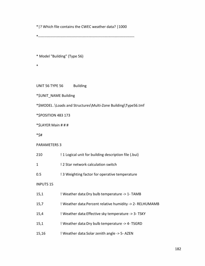
182

*|? Which file contains the CWEC weather data? |1000

*------------------------------------------------------------------------------

* Model "Building" (Type 56)

*

UNIT 56 TYPE 56 Building

*$UNIT_NAME Building

*$MODEL .\Loads and Structures\Multi-Zone Building\Type56.tmf

*$POSITION 483 173

*$LAYER Main # # #

*$#

PARAMETERS 3

210 ! 1 Logical unit for building description file (.bui)

1 ! 2 Star network calculation switch

0.5 ! 3 Weighting factor for operative temperature

INPUTS 15

15,1 ! Weather data:Dry bulb temperature -> 1- TAMB

15,7 ! Weather data:Percent relative humidity -> 2- RELHUMAMB

15,4 ! Weather data:Effective sky temperature -> 3- TSKY

15,1 ! Weather data:Dry bulb temperature -> 4- TSGRD

15,16 ! Weather data:Solar zenith angle -> 5- AZEN

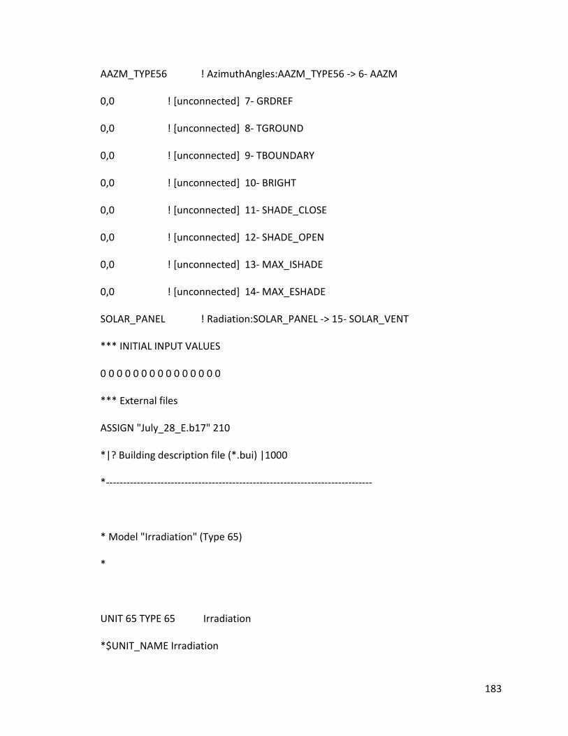
183

AAZM_TYPE56 ! AzimuthAngles:AAZM_TYPE56 -> 6- AAZM

0,0 ! [unconnected] 7- GRDREF

0,0 ! [unconnected] 8- TGROUND

0,0 ! [unconnected] 9- TBOUNDARY

0,0 ! [unconnected] 10- BRIGHT

0,0 ! [unconnected] 11- SHADE_CLOSE

0,0 ! [unconnected] 12- SHADE_OPEN

0,0 ! [unconnected] 13- MAX_ISHADE

0,0 ! [unconnected] 14- MAX_ESHADE

SOLAR_PANEL ! Radiation:SOLAR_PANEL -> 15- SOLAR_VENT


0 0 0 0 0 0 0 0 0 0 0 0 0 0 0

*** External files

ASSIGN "July_28_E.b17" 210

*|? Building description file (*.bui) |1000

*------------------------------------------------------------------------------

* Model "Irradiation" (Type 65)

*

UNIT 65 TYPE 65 Irradiation

*$UNIT_NAME Irradiation

184


*$POSITION 317 223

*$LAYER Main # # #

PARAMETERS 12

1 ! 1 Nb. of left-axis variables

1 ! 2 Nb. of right-axis variables

0 ! 3 Left axis minimum

3600 ! 4 Left axis maximum

0 ! 5 Right axis minimum

3600 ! 6 Right axis maximum

1 ! 7 Number of plots per simulation

12 ! 8 X-axis gridpoints

0 ! 9 Shut off Online w/o removing

-1 ! 10 Logical unit for output file

0 ! 11 Output file units

0 ! 12 Output file delimiter

INPUTS 2

IT_H_0_0 ! Radiation:IT_H_0_0 ->Left axis variable

IB_H_0_0 ! Radiation:IB_H_0_0 ->Right axis variable


IT_H_0_0 IB_H_0_0

LABELS 3

185

"Total Incident Solar Radition [kJ/hr m²]"

"Beam Incident Solar Radition [kJ/hr m²]"

"Irradition"

*------------------------------------------------------------------------------

* Model "Temperature" (Type 65)

*

UNIT 66 TYPE 65 Temperature

*$UNIT_NAME Temperature


*$POSITION 449 298

*$LAYER Main # # #

PARAMETERS 12

1 ! 1 Nb. of left-axis variables

2 ! 2 Nb. of right-axis variables

-20 ! 3 Left axis minimum

35 ! 4 Left axis maximum

-20 ! 5 Right axis minimum

35 ! 6 Right axis maximum

1 ! 7 Number of plots per simulation

12 ! 8 X-axis gridpoints

0 ! 9 Shut off Online w/o removing

-1 ! 10 Logical unit for output file

186

0 ! 11 Output file units

0 ! 12 Output file delimiter

INPUTS 3

15,1 ! Weather data:Dry bulb temperature ->Left axis variable

56,16 ! Building: 16- TAIR_DOME ->Right axis variable-1

56,1 ! Building: 1- TAIR_WATER_TANK ->Right axis variable-2


Tamb DOME DOME

LABELS 3

"Temperatures [deg C]"

"Temperatures [deg C]"

"Temperatures"

*------------------------------------------------------------------------------

* Model "System_Printer" (Type 25)

*

UNIT 9 TYPE 25 System_Printer

*$UNIT_NAME System_Printer

*$MODEL \Trnsys17\Studio\lib\System_Output\Type25a.tmf

*$POSITION 328 106

*$LAYER OutputSystem #

PARAMETERS 10

STEP ! 1 Printing interval

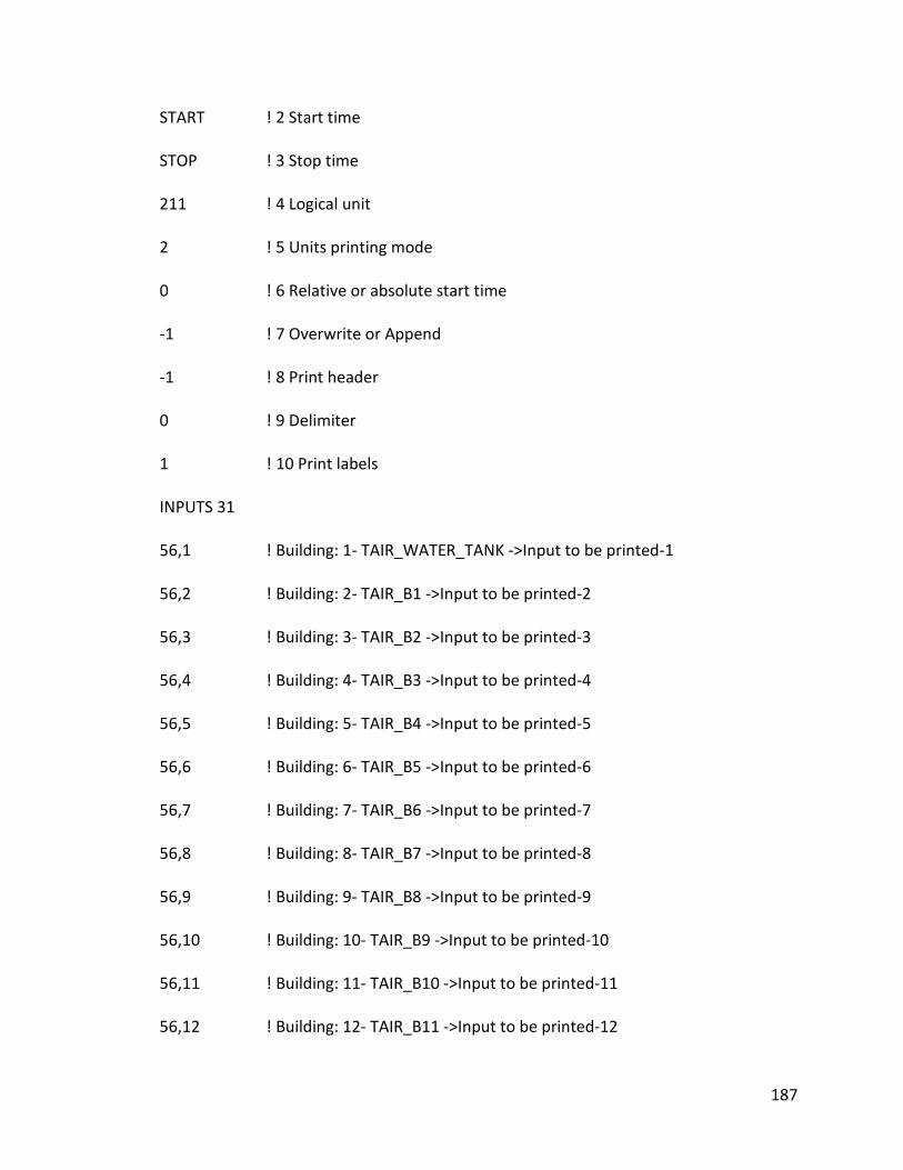
187

START ! 2 Start time

STOP ! 3 Stop time

211 ! 4 Logical unit

2 ! 5 Units printing mode

0 ! 6 Relative or absolute start time

-1 ! 7 Overwrite or Append

-1 ! 8 Print header

0 ! 9 Delimiter

1 ! 10 Print labels

INPUTS 31

56,1 ! Building: 1- TAIR_WATER_TANK ->Input to be printed-1

56,2 ! Building: 2- TAIR_B1 ->Input to be printed-2











188




56,16 ! Building: 16- TAIR_DOME ->Input to be printed-16

56,17 ! Building: 17- TAIR_DOOR_BOTTOM ->Input to be printed-17

56,18 ! Building: 18- TAIR_C6 ->Input to be printed-18













IT_S_0_50 ! Radiation:IT_S_0_50 ->Input to be printed-31


TAIR_WATER_TANK T_B1 T_B2 T_B3 T_B4 T_B5 T_B6 T_B7 T_B8 T_B9 T_B10 T_B11

T_B12 T_B13 T_B14 T_DOME T_DOOR T_C6 T_C5 T_C4 T_C3 T_C2 T_C1 T_C14 T_C8

189

T_C9 T_C10 T_C11 T_C12 T_C13 SOLAR_VENT_RAD

*** External files

ASSIGN "Type25a.txt" 211

*|? Which file should contain the printed results? You can use the deck filename by

entering "***", e.g. "***.out", or "***.dat" |1000

*-----------------------------------------------------------------------------

END

190

Appendix C: Arduino Program

/*-(Import required libraries)-*/

#include <Time.h>

#include <Wire.h>

#include <SPI.h>

#include <SD.h>

#include <OneWire.h>

#include <DallasTemperature.h>

#include <DHT.h>

#include <LowPower.h>

#include <DS3232RTC.h> //source: https://github.com/JChristensen/DS3232RTC

/*-( Declare Constants )-*/

#define ECHO_TO_SERIAL 1 // echo data to serial port for SD card reader

const int wakeUpPin = 2;

#define greenLEDpin 3

#define redLEDpin 4

#define RELAY_1 5

#define DHT1PIN 6 //DHT22 humidity and temperature sensor on digital pin 6

#define DHT2PIN 7 //DHT22 humidity and temperature sensor on digital pin 7

#define ONE_WIRE_BUS 8 // All thermocouples using 1-Wire protocol on digital pin 8

#define RELAY_2 9

const int chipSelect = 10;

#define DHTTYPE DHT22

#define RELAY_ON HIGH

#define RELAY_OFF LOW

#define resolution 5

//*-( Declare objects )-*

DHT dht1(DHT1PIN, DHTTYPE);

DHT dht2(DHT2PIN, DHTTYPE);

OneWire oneWire(ONE_WIRE_BUS);

DallasTemperature sensors(&oneWire);

//hardware address of each thermocouple

byte tc1[8] = {0x3B, 0x1A, 0x30, 0x18, 0x0, 0x0, 0x0, 0x96}; //#1

byte tc2[8] = {0x3B, 0x41, 0x2D, 0x18, 0x0, 0x0, 0x0, 0xD0}; //#2

byte tc3[8] = {0x3B, 0xF2, 0x32, 0x18, 0x0, 0x0, 0x0, 0x9D}; //#3

byte tc4[8] = {0x3B, 0x51, 0x2D, 0x18, 0x0, 0x0, 0x0, 0x8B}; //#4

byte tc5[8] = {0x3B, 0xC0, 0x27, 0x18, 0x0, 0x0, 0x0, 0xB0}; //#5

byte tc6[8] = {0x3B, 0xE0, 0x27, 0x18, 0x0, 0x0, 0x0, 0x06}; //#6

191

byte tc7[8] = {0x3B, 0x05, 0x2E, 0x18, 0x0, 0x0, 0x0, 0x37}; //#7

byte tc8[8] = {0x3B, 0xC4, 0x2F, 0x18, 0x0, 0x0, 0x0, 0x52}; //#8

byte tc9[8] = {0x3B, 0x07, 0x32, 0x18, 0x0, 0x0, 0x0, 0x04}; //#9

byte tc10[8] = {0x3B, 0xD3, 0x2B, 0x18, 0x0, 0x0, 0x0, 0x93}; //#10

byte tc11[8] = {0x3B, 0x47, 0x2B, 0x18, 0x0, 0x0, 0x0, 0xFE}; //#11

byte tc12[8] = {0x3B, 0xA2, 0x2B, 0x18, 0x0, 0x0, 0x0, 0x3C}; //#12

byte tc13[8] = {0x3B, 0x2F, 0x30, 0x18, 0x0, 0x0, 0x0, 0x90}; //#13

byte tc14[8] = {0x3B, 0xC7, 0x2F, 0x18, 0x0, 0x0, 0x0, 0x0B}; //#14

byte tc15[8] = {0x3B, 0x12, 0x2C, 0x18, 0x0, 0x0, 0x0, 0x6A}; //#15

byte tc16[8] = {0x3B, 0x6E, 0x6F, 0x18, 0x0, 0x0, 0x0, 0x28}; //#16

byte tc18[8] = {0x3B, 0x31, 0x76, 0x18, 0x0, 0x0, 0x0, 0xAD}; //#18

byte tc19[8] = {0x3B, 0x27, 0x32, 0x18, 0x0, 0x0, 0x0, 0xB2}; //#19

byte tc20[8] = {0x3B, 0xB2, 0x6C, 0x18, 0x0, 0x0, 0x0, 0xDF}; //#20


byte tc22[8] = {0x3B, 0x19, 0x6C, 0x18, 0x0, 0x0, 0x0, 0x7B}; //#22


//SD CARD

File logfile;

/*-(Declare Variables)-*/

time_t t;

int nextLoop;

int Fan_1;

int Fan_2;

/****** SETUP: RUNS ONCE ******/

void setup()

{

Serial.begin(9600);

Serial.println("Relays off to start");

//(set pins as outputs )

pinMode(RELAY_1, OUTPUT);

pinMode(RELAY_2, OUTPUT);

//( Initialize Pins so relays are inactive at reset)

digitalWrite(RELAY_1, RELAY_OFF);


Fan_1 = 0;

Fan_2 = 0;

Serial.println();

Wire.begin();

setSyncProvider(RTC.get);

Serial.print("Initializing SD card...");

pinMode(10, OUTPUT);

192

pinMode(wakeUpPin, INPUT);

// see if the card is present and can be initialized:

if (!SD.begin(chipSelect)) {

Serial.println("Card failed, or not present");

// don't do anything more:

return;

}

Serial.println("card initialized.");

//define filename

char filename[] = "LOGGER00.CSV";

for (uint8_t i = 0; i < 100; i++) {

filename[6] = i / 10 + '0';

filename[7] = i % 10 + '0';

Serial.println(filename);

if (!SD.exists(filename)) {

// only open a new file if it doesn't exist

logfile = SD.open(filename, FILE_WRITE);

break; // leave the loop!

}

}

if (!logfile) {

error("could not create file");

}

t = RTC.get();

Serial.print("Logging to: ");

Serial.println(filename);

logfile.println("date,hour,min,sec,tc-1,tc-2,tc-3,tc-4,tc-5,tc-6,tc-7,tc-8,tc-9,tc-10,tc-11,tc-

12,tc-13,tc-14,tc-15,tc-16,tc-18,tc-19,tc-20,tc-21,tc-22,tc-23,dht-1h,dht-1t,dht-2h,dht-

2t,Fan_1, Fan_2");

#if ECHO_TO_SERIAL

Serial.println("date,hour,min,sec,tc-1,tc-2,tc-3,tc-4,tc-5,tc-6,tc-7,tc-8,tc-9,tc-10,tc-

11,tc-12,tc-13,tc-14,tc-15,tc-16,tc-18,tc-19,tc-20,tc-21,tc-22,tc-23,dht-1h,dht-1t,dht-

2h,dht-2t,Fan_1, Fan_2");

#endif

pinMode(redLEDpin, OUTPUT);

pinMode(greenLEDpin, OUTPUT);

nextLoop = ((minute(RTC.get()) / resolution) + 1) * resolution;

if (nextLoop >= 60) {

nextLoop -= 60;

}

Serial.print(RTC.temperature());

193

Serial.print(",");

Serial.print(RTC.oscStopped());

Serial.print(",");

Serial.println(nextLoop);

sensors.begin();

dht1.begin();

dht2.begin();

}

/****** LOOP: RUNS CONSTANTLY ******/

void loop()

{

t = RTC.get();

sensors.requestTemperatures(); // Send the command to get temperatures

digitalWrite(greenLEDpin, HIGH);

logfile.print(year(t), DEC);

logfile.print("/");

logfile.print(month(t), DEC);

logfile.print("/");

logfile.print(day(t), DEC);

logfile.print(",");

logfile.print(hour(t), DEC);

logfile.print(",");

logfile.print(minute(t), DEC);

logfile.print(",");

logfile.print(second(t), DEC);

logfile.print(",");

logfile.print(sensors.getTempC(tc1)); logfile.print(",");
















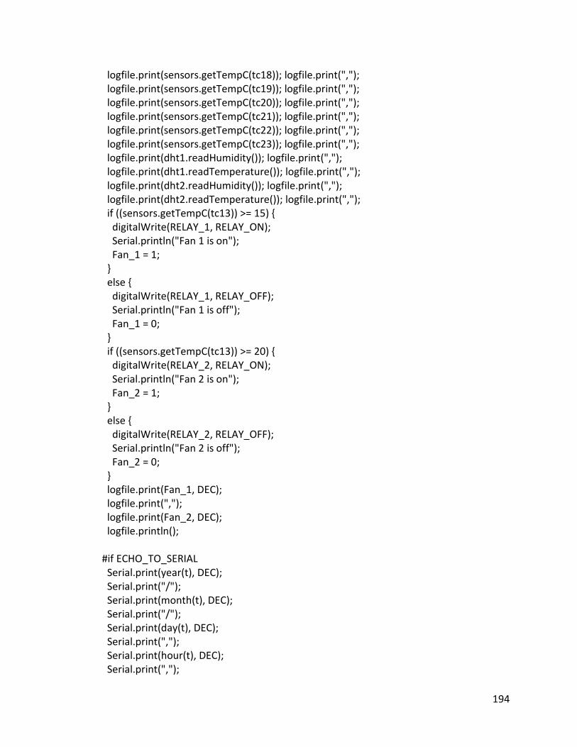
194







logfile.print(dht1.readHumidity()); logfile.print(",");

logfile.print(dht1.readTemperature()); logfile.print(",");

logfile.print(dht2.readHumidity()); logfile.print(",");

logfile.print(dht2.readTemperature()); logfile.print(",");

if ((sensors.getTempC(tc13)) >= 15) {

digitalWrite(RELAY_1, RELAY_ON);

Serial.println("Fan 1 is on");

Fan_1 = 1;

}

else {


Serial.println("Fan 1 is off");

Fan_1 = 0;

}

if ((sensors.getTempC(tc13)) >= 20) {

digitalWrite(RELAY_2, RELAY_ON);

Serial.println("Fan 2 is on");

Fan_2 = 1;

}

else {


Serial.println("Fan 2 is off");

Fan_2 = 0;

}

logfile.print(Fan_1, DEC);

logfile.print(",");

logfile.print(Fan_2, DEC);

logfile.println();

#if ECHO_TO_SERIAL

Serial.print(year(t), DEC);

Serial.print("/");

Serial.print(month(t), DEC);

Serial.print("/");

Serial.print(day(t), DEC);

Serial.print(",");

Serial.print(hour(t), DEC);

Serial.print(",");

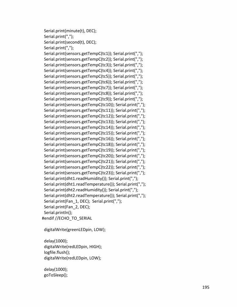
195

Serial.print(minute(t), DEC);

Serial.print(",");

Serial.print(second(t), DEC);

Serial.print(",");

Serial.print(sensors.getTempC(tc1)); Serial.print(",");






















Serial.print(dht1.readHumidity()); Serial.print(",");

Serial.print(dht1.readTemperature()); Serial.print(",");

Serial.print(dht2.readHumidity()); Serial.print(",");

Serial.print(dht2.readTemperature()); Serial.print(",");

Serial.print(Fan_1, DEC); Serial.print(",");

Serial.print(Fan_2, DEC);

Serial.println();

#endif //ECHO_TO_SERIAL

digitalWrite(greenLEDpin, LOW);

delay(1000);

digitalWrite(redLEDpin, HIGH);

logfile.flush();

digitalWrite(redLEDpin, LOW);

delay(1000);

goToSleep();

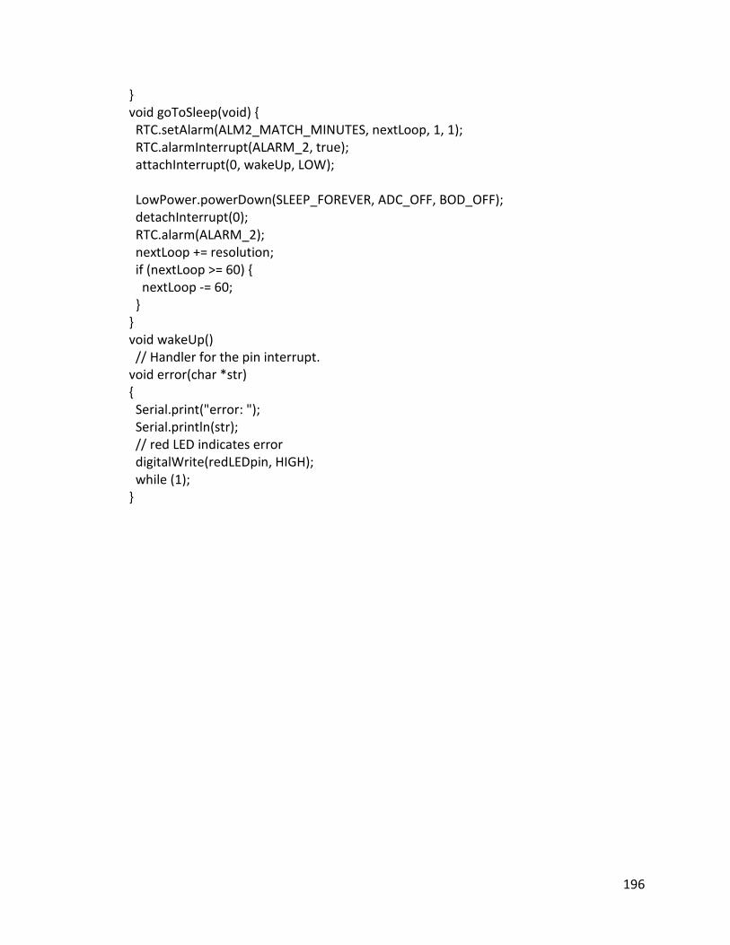
196

}

void goToSleep(void) {

RTC.setAlarm(ALM2_MATCH_MINUTES, nextLoop, 1, 1);

RTC.alarmInterrupt(ALARM_2, true);

attachInterrupt(0, wakeUp, LOW);

LowPower.powerDown(SLEEP_FOREVER, ADC_OFF, BOD_OFF);

detachInterrupt(0);

RTC.alarm(ALARM_2);

nextLoop += resolution;

if (nextLoop >= 60) {

nextLoop -= 60;

}

}

void wakeUp()

// Handler for the pin interrupt.

void error(char *str)

{

Serial.print("error: ");

Serial.println(str);

// red LED indicates error

digitalWrite(redLEDpin, HIGH);

while (1);

}

experimental and modelling study of a geodesic dome solar

Documents