section 2. rock physics
TRANSCRIPT
Fred J. Hilterman
Distinguished Instructor Short Course • 2-1
Section 2. Rock Physics
Objective:
1. Illustrate velocity dependence and sensitivity to elastic constants and environmental factors
2. Examine rock-property transforms
3. Estimate P-wave and S-wave velocities when pore-fluid and/or porositychanges
One of the primary goals of amplitude interpretation is to determine whether a water-saturated rock or a hydrocarbon-saturated rock generated the reflection of interest. Inorder to accomplish this task, an estimate of the difference in rock properties betweenthe water-saturated and hydrocarbon-saturated states is required. Thus, a few basic rela-tionships of rock physics are necessary. There are both empirical and theoretical rela-tionships between seismic rock properties and elastic constants that will be called upon,as well as wave-propagation models.
The work presented in these notes has drawn heavily from two excellent references.The first is a tutorial article by Castagna et al. (1993): “Rock Physics—The LinkBetween Rock Properties and AVO Response.” The second is a book for those who wantdetailed solutions to various rock-property transforms but don’t want to wade throughthe messy math. The book is written by Mavko et al. (1998): The Rock PhysicsHandbook—Tools for Seismic Analysis in Porous Media. In addition, the two SEG reprintvolumes, Seismic Acoustic Velocities in Reservoir Rocks, compiled by Wang and Nur(1992), provide easy access to classic articles on petrophysics.
2A. P-waves, S-waves, Density, and Poisson’s Ratio
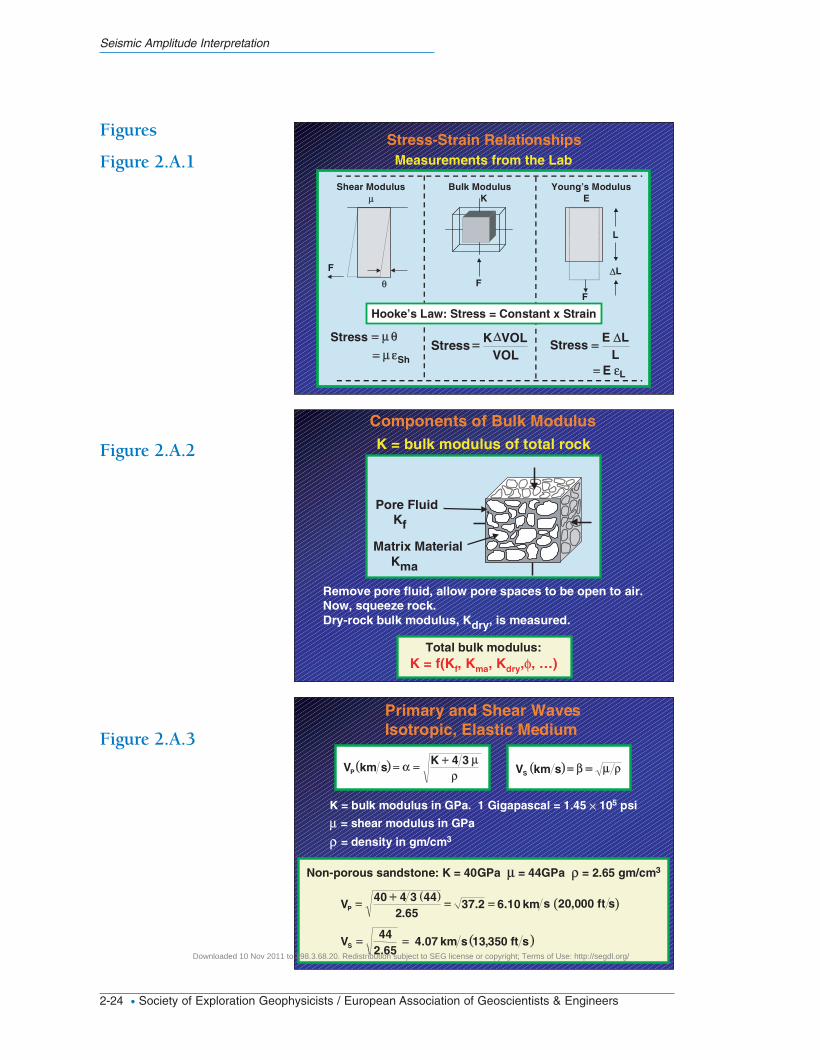
Before a theory can be formulated for wave motion in a medium, a relationship betweenstress and strain is needed. For waves of infinitesimal amplitude, Hooke’s empirical lawsupplies this relationship. The three most commonly used elastic constants to quantita-tively describe the strength of a body are the shear (µ), bulk (K), and Young’s (E) mod-uli. The cartoon in Fig.2.A.1 illustrates the hypothetical experiments that measure theseelastic constants. In reality, it is difficult to measure the shear modulus (rigidity) asdescribed in the figure and obtain useable results. However, the other two moduli mea-surements are conducive to lab measurements. As an example, if the bulk modulus of asolid rubber ball were desired, a simple experiment could be conducted. Measure thediameter of the ball and then dive into a deep lake and measure the ball’s diameter atthe depth of 500 ft (150 m). At 500 ft, the stress (or hydrostatic pressure) is approxi-mately 230 psi (1590 kPa). Knowing the change in stress and the change in volume, thebulk modulus can be computed. Young’s modulus is normally measured on thin rodlikespecimens.
The experiments described in Fig. 2.A.1 would yield the necessary elastic constantsfor developing a wave theory if the material were nonporous. For porous material, the
04_Section 02_v2New.qxd 12/3/09 2:30 PM Page 2-1
Downloaded 10 Nov 2011 to 198.3.68.20. Redistribution subject to SEG license or copyright; Terms of Use: http://segdl.org/
bulk modulus needs to be separated into its components (Fig. 2.A.2). The bulk-modu-lus components selected in the figure are pertinent to Gassmann’s wave propagationtheory, which will be introduced later. The three components are the pore-fluid (Kf),matrix-material (Kma), and dry-rock (Kdry) bulk moduli. If the pore fluid and matrixmaterial (grains) are known from well-log measurements, their associated bulk modulican be estimated fairly easily. The dry-rock bulk modulus is a bit more difficult to comeby and other relationships will be developed to assist in estimating it.
In Fig. 2.A.3, two of the rock moduli are related to the P-wave and S-wave veloci-ties. Throughout these notes, the Greek letters α and β will be used interchangeablywith VP and VS to refer to the P-wave (primary or compressional) and S-wave (shear)velocities, respectively. While current convention requires that the metric system beemployed in geophysical literature, many of the graphs and figures shown in thesenotes are reproduced from literature and are annotated in the English system. If thebulk moduli of the rock are expressed in gigapascals (GPa) and the density in gm/cc(gm/cm3), then the resulting velocity is expressed in km/s. The bottom of the figurecontains an example with appropriate units for nonporous sandstone.
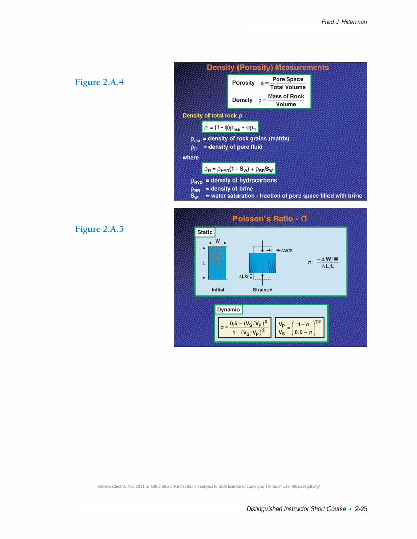
In order to solve for velocities in the equations of Fig. 2.A.3, the density, ρ, isrequired. Density is expressed as a function of porosity, φ, as shown in Fig. 2.A.4. Thebulk density of the rock, ρ, is related to the matrix (grains) and pore-fluid densities. Asthe bulk density depends on porosity, the fluid density depends on the water saturation,SW, which is the percentage of the pore space filled with water (brine). What is not indi-cated is that most rocks are composed of more than one mineral. Thus, the matrixdensity, ρma, needs to be expressed as a volumetric average of the individual mineraldensities.
During rock-squeezing experiments in the lab, Poisson’s ratio, σ, can also be mea-sured as shown in Fig. 2.A.5 (static measurement). Poisson’s ratio, which is Koefoed’slithologic identifier, is simply the negative ratio of the transverse strain to the longitudi-nal strain. Normally, however, geophysicists express Poisson’s ratio as a function of theP-wave and S-wave velocities (dynamic measurement).
For isotropic media, the value of Poisson’s ratio falls between 0.0 and 0.5. The twoextremes are useful to examine. When the strained volume is equal to the initial vol-ume, Poisson’s ratio is 0.5. This is the case for fluids, which include water, air, and oil.In addition, for the first hundred feet beneath the ocean bottom, Poisson’s ratioapproaches 0.5 for recent sediments. For those involved in physical modeling experi-ments, rubber has a Poisson’s ratio very close to 0.5. The other extreme occurs whenthe strained volume has no transverse strain, or as Mike Graul has quoted, “It has zerofatticity; it doesn’t get fat as you squeeze it vertically.” What doesn’t get fatter when yousqueeze it? A sponge! In exploration geophysics, this occurs in some sense when wateris replaced with gas in the pores. Poisson’s ratio of the rock always decreases when gasis substituted for water in the pore space.
Substantial differences between the static and dynamic measurements of Poisson’sratio for the same rock are reported in literature. The dynamic Poisson’s ratio is normal-ly higher. Wang offered an explanation for these discrepancies. In the dynamic measure-ments, the propagating waves have strain amplitudes smaller than 10-6, while the staticmeasurements (squeezing in a vise) have strain amplitudes greater than 10-3. That is,
Seismic Amplitude Interpretation
2-2 • Society of Exploration Geophysicists / European Association of Geoscientists & Engineers
04_Section 02_v2New.qxd 12/3/09 2:30 PM Page 2-2
Downloaded 10 Nov 2011 to 198.3.68.20. Redistribution subject to SEG license or copyright; Terms of Use: http://segdl.org/
static measurements squeeze the rock more than dynamic methods. Most sedimentaryrocks have pores or cracks that are elongated (not spherical) and the propagating wavesin the dynamic method do not squeeze these cracks closed. Thus, the rock appears tobe stronger (less compressible) than in the situation where the cracks close. In the staticmethod, the cracks close and the rock will appear to have a lower strength. If the exper-iments are conducted at higher confining pressures so that the cracks are closed at thebeginning of the experiment, then static and dynamic measurements of Poisson’s ratioapproach one another.
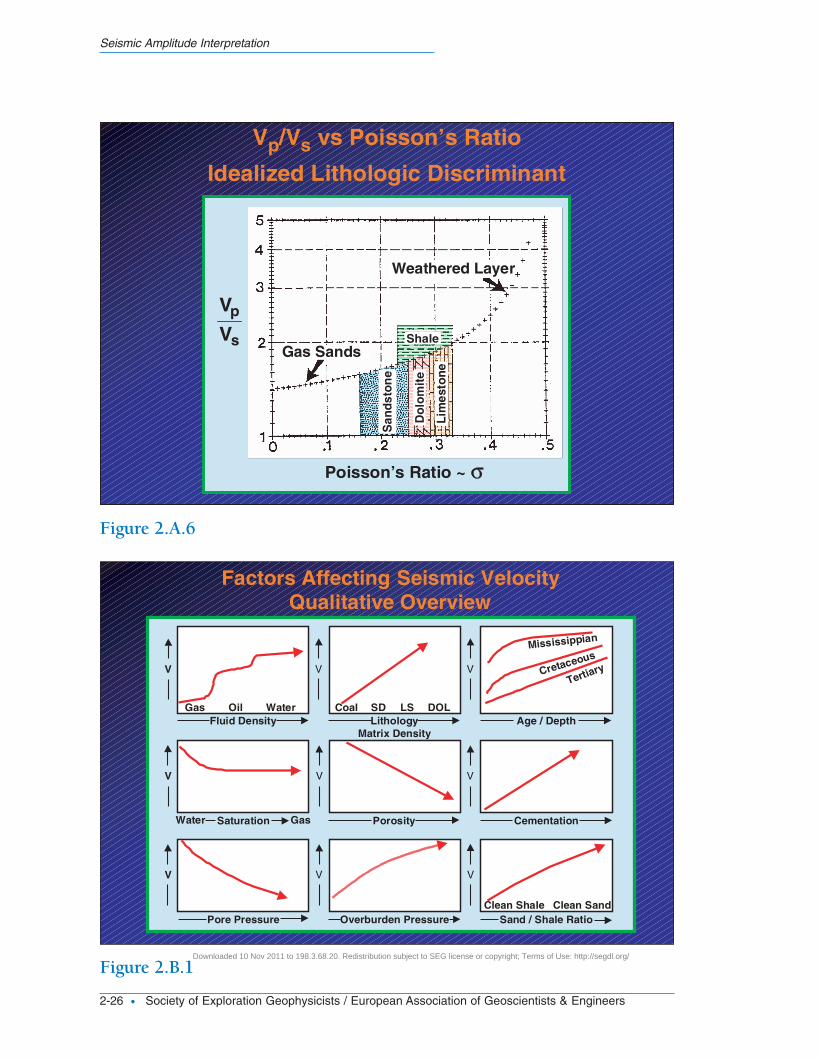
A brief preview of the significance of VP/VS or Poisson’s ratio for discriminating dif-ferent lithologies is shown in Fig. 2.A.6. This is an idealized plot. At a particular depth,shales tend to have a Poisson’s ratio that is larger than that for sands, especially gas-sat-urated sands. As the depth of investigation becomes shallower, sand and shale Poisson’sratio values move toward 0.5. Also, the sand and shale trends tend to overlap more.Conversely, as the depth of investigation increases, the sand and shale trends tend toseparate and have lower Poisson’s ratio values—with sand still having a Poisson’s ratiolower than shale does. However, with changes of depth, Poisson’s ratio for limestoneand dolomite does not vary as much as it does for sandstone and shale.
2B. Establishing Regional and Local Rock-Property Trends
Whenever an amplitude anomaly is recognized on a seismic section, the trick is to dis-tinguish what rock-property variation caused the amplitude change. In order to assist inthis decision, rules-of-thumb are desired on how velocity is affected by changes in (a)elastic moduli, (b) densities, and (c) various environmental conditions (Fig. 2.B.1). Afew of the primary factors affecting velocity are as follows.
Fluid Density—For unconsolidated clastics, pore-fluid variations can significantlychange the velocity of the rock. As the pore-fluid density increases, the rock’s velocityincreases. However, for well-consolidated rocks, porosity variations become more signif-icant than pore-fluid variations for changing the rock’s velocity.
Matrix Density—Denser rocks normally have a higher velocity than lighter rocks.Density variations are often the primary component of the reflection coefficient for shal-low wet unconsolidated rocks.
Age/Depth—Age, by itself, does not affect the rock’s velocity. It is all the other factorsthat occur over time, such as increased cementation, loss of porosity, compaction, anddiagenetic changes. High-velocity rocks tend to have a rapid increase in velocity withdepth for the first 3000 ft (900 m) as the micro-cracks close. Then, the velocity increas-es slowly with depth until the velocity approaches the terminal zero-porosity end mem-ber. For unconsolidated rocks, velocity tends to increase linearly with depth, or, moreexactly, with increases in effective pressure, which is discussed later.
Water Saturation—As mentioned, if the pore-fluid density increases, the P-wavevelocity increases. However, this increase in velocity is not necessarily linear with theincrease of pore-fluid density. For shallow unconsolidated sediments, a small percentageof gas in the pores significantly decreases the velocity of the rock compared with thewater-saturated state. However, once the rock is saturated with 5–10% gas, further gassaturation has little effect on the rock’s velocity. Unfortunately, this means that econom-
Fred J. Hilterman
Distinguished Instructor Short Course • 2-3
04_Section 02_v2New.qxd 12/3/09 2:30 PM Page 2-3
Downloaded 10 Nov 2011 to 198.3.68.20. Redistribution subject to SEG license or copyright; Terms of Use: http://segdl.org/
ic gas reservoirs have almost the same P-wave seismic amplitude as a depleted reservoir.Porosity—There are numerous empirical formulas that log analysts have derived
over the years to evaluate a reservoir’s porosity in terms of sonic-log traveltime (inverseof velocity). Porosity alters both the density of a rock and its elastic moduli, such thatporosity increases yield velocity decreases.
Cementation—Cementation of the grains, which normally increases with age,reduces the porosity and increases the elastic moduli of the rock. Thus cementationincreases the velocity of the rock.
Pore Pressure and Overburden Pressure—It is necessary to consider overburden pres-sure and pore pressure together when analyzing velocity. The overburden pressure on aformation results from the total weight of the rock above it, including the fluid in therock. If the rock has hydrostatic communication with the surface, then the pore pres-sure in the rock is equal to the pressure at the base of a column of brine that has aheight equal to the formation’s depth (hydrostatic pressure). If the overburden pressureis increased while holding the pore pressure constant, the solid matrix will be squeezedcloser together and the rock’s elastic moduli increase while the density changes little.Similarly, if the pore pressure increases while the overburden pressure remains thesame, the pore fluid tends to support more of the overburden and the rock appearsweaker and the formation has a lower velocity. This last scenario is an abnormally pres-sured formation. For our purposes, the overburden pressure minus the pore pressure iscalled the effective pressure. If the effective pressure is held constant, then no apparentchange in velocity is recognized. With an overburden pressure gradient of 1 psi/ft and apore pressure gradient of 0.47 psi/ft, the effective pressure on the rock increases at 0.53psi/ft. Thus velocity generally increases with depth.
Shale Content—Normally, the P-wave velocity decreases as the shale content isincreased. However, this is not always the case. The direction of the velocity changedepends on how shale enters the rock: fills the pores, breaches the grain contacts, orreplaces part of the skeleton.
From the factors listed above, which one influences velocity the most? Generally,the dominant factors that influence velocity must be determined for an individual area.The different factors are introduced as either filters or variables in trend analyses forregional and local amplitude interpretations. A trend example from the Gulf of Mexico(GOM), which contains essentially unconsolidated clastic sediments, illustrates the con-cept by filtering the samples based on lithology and the presence of abnormal pressure.Effective pressure is a variable approximated by depth. Velocity and density trends forboth sand and shale are desired for quantifying future amplitude interpretations.
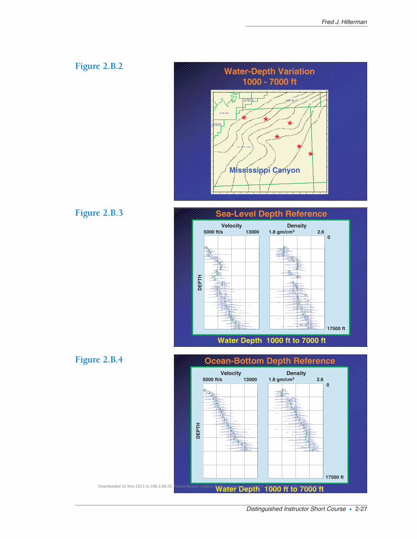
Sea-Level Versus Ocean-Bottom Datum
The six well locations illustrated in Fig. 2.B.2 have water depths ranging from 1000to 7000 ft (300 to 2000 m). Velocity and density histogram trends were developed fromthese six wells and they are illustrated in Fig. 2.B.3. A histogram trend contains statisti-cal analyses at 500-ft (150-m) depth intervals from a specified datum to approximately18,000 ft (6000 m) beneath the datum. Velocity and density samples from well-logcurves were taken at 1-ft intervals. All lithologies were included and the datum was setat sea level. The vertical line near the maximum-frequency point for each 500-ft his-
Seismic Amplitude Interpretation
2-4 • Society of Exploration Geophysicists / European Association of Geoscientists & Engineers
04_Section 02_v2New.qxd 12/3/09 2:30 PM Page 2-4
Downloaded 10 Nov 2011 to 198.3.68.20. Redistribution subject to SEG license or copyright; Terms of Use: http://segdl.org/
togram represents the average value. The small red dot represents a recomputed averageafter samples more than one standard deviation from the original average were omitted.It is difficult to predict a reliable trend for either velocity or density from the plots inFig. 2.B.3. The histograms are too disjointed from one depth to the next to be consid-ered reliable. The first impulse is to rerun the data and produce separate histogramtrends for sand and shale. However, this is not the primary factor to consider for devel-oping reliable trend curves in this area.
The same six well-log curves were reexamined, but with the depth datum set atocean bottom (Fig 2.B.4). More continuous and thus reliable trends are produced.Obviously, velocity and density trend curves to be used in amplitude interpretationshould be referenced from the ocean bottom. Why?
Effective Pressure
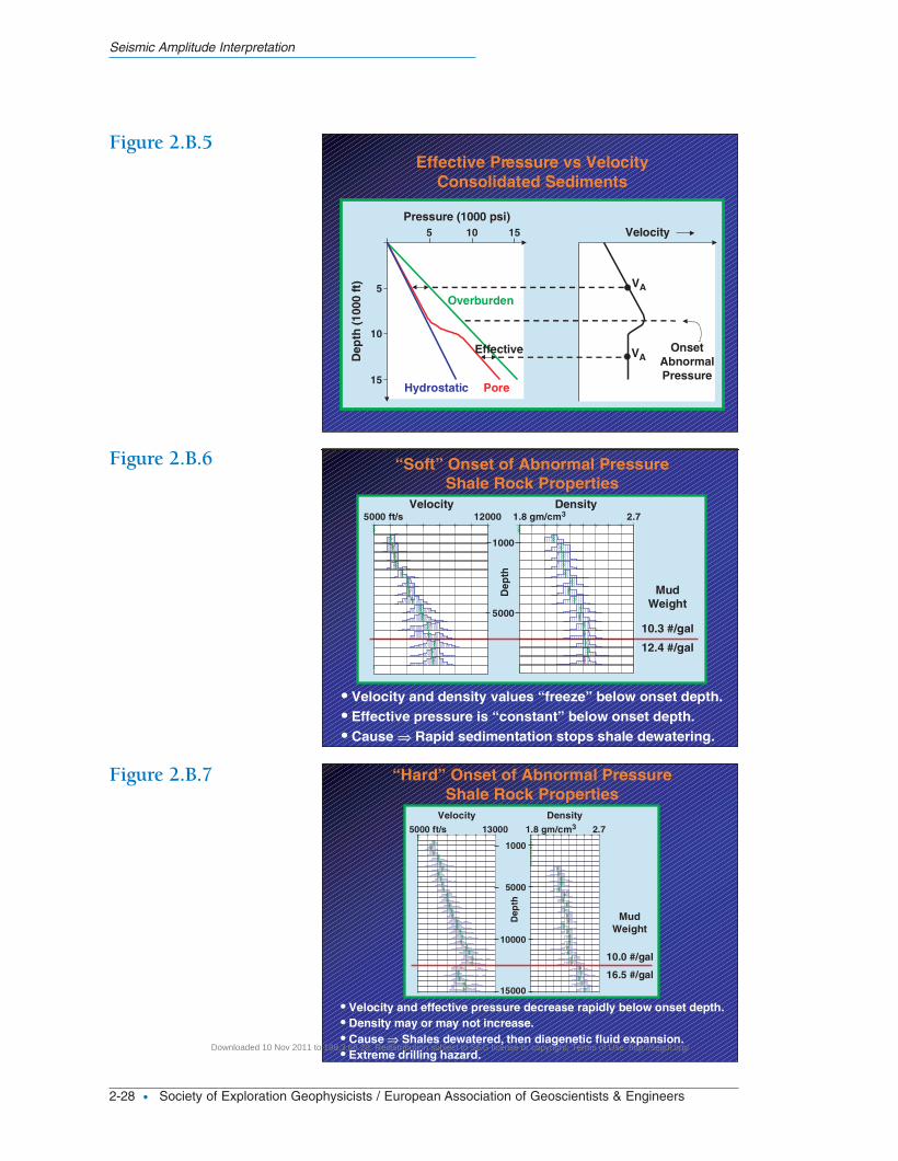
As mentioned earlier, the effective pressure can be a primary factor controlling velocity.The effective pressure is zero in the water column and does not change until sedimentsare reached. The empirical relationship of effective pressure to in-situ velocity is car-tooned in Fig. 2.B.5. The effective pressure, which is approximately the overburdenpressure minus the pore pressure, increases linearly until the onset of abnormal porepressure is reached (at 7500 ft [2300 m] in the figure). The velocity profile also increas-es linearly to the onset of abnormal pressure. Below the onset of abnormal pore pres-sure, the fluid in the pores begins to support the overburden rock, and the effectivepressure decreases. The two points labeled as VA on the velocity profile have the sameeffective pressure and thus have approximately the same in-situ velocity. As a side note,it was this empirical velocity-to-effective-pressure relationship, which can be deter-mined from seismic interval-velocity analyses, that formed the basis of predicting mud-weight programs for drilling engineers (Hottman and Johnson, 1965; Pennebaker, 1968;Dutta and Levin, 1987). This is a very simplistic relationship of interval velocity toeffective pressure that needs to be adjusted slightly for actual field conditions.
The expected rock properties beneath the onset of abnormal geopressure dependnot only on the effective pressure but also on the environmental reasons for the abnor-mal pressure. Often, the environmental reasons can be inferred by the change in theshape of the effective pressure curve. In drilling terminology, these changes in effective-pressure curves are called soft and hard onsets of abnormal geopressure.
A soft onset is illustrated with shale histogram trends from a single well in thesouthern portion of offshore Louisiana, Vermilion Block 395 (Fig. 2.B.6). At the 6500-ft(2000-m) depth, the onset of abnormal pressure occurred and the mud weight at thisdepth was gradually increased from 10.3 lbs/gal to 12.4 lbs/gal at the bottom of thehole. The velocity and density values beneath 6500-ft depth are essentially the same asthe values at 6500 ft. This indicates that the effective pressure is constant over thedepth interval beneath the onset of abnormal pressure. This type of overpressure com-monly occurs when the pore fluid trapped by low-permeability shale is squeezed by theweight of newly deposited sediments. This abnormal pressure is referred to as under-compaction or compaction disequilibrium (Bowers, 1995).
A hard onset of abnormal pressure is depicted by the shale histogram trend curvesin Fig. 2.B.7. Above the onset of abnormal pressure, the shale rock-property trends are
Fred J. Hilterman
Distinguished Instructor Short Course • 2-5
04_Section 02_v2New.qxd 12/3/09 2:30 PM Page 2-5
Downloaded 10 Nov 2011 to 198.3.68.20. Redistribution subject to SEG license or copyright; Terms of Use: http://segdl.org/
essentially the same as the soft-onset trend curves, but they differ dramatically below. Inthe soft onset, the density values beneath the onset have a somewhat predictable trend,but in the hard onset, density values may increase, decrease, or remain constant. Also,the velocity drops significantly when abnormal pressure is reached in the hard-onsetcase. Bower emphasized the importance of distinguishing this mechanism of overpres-sure from undercompaction. This overpressure can be generated by fluid expansionsuch as heating, hydrocarbon maturation, and expulsion/expansion of intergranularwater during clay diagenesis. This is an unloading mechanism, and normally the effec-tive pressure decreases more than is predicted from interval velocity. The rock under-goes a plastic and not an elastic rebound.
These significant changes in the velocity and density trends suggest that a horizonmap indicating the depth to the onset of abnormal pressure should be incorporated intoall amplitude interpretations.
The different mechanisms for generating abnormal geopressure were also correlatedto stratigraphy by Verm et al. (1998). The study used over 2700 wells and includedGOM regional trend analyses. The maps in Fig. 2.B.8 indicate a strong correlationbetween the depth to abnormal-pressure onset and the major sand deposits. In thenorthern portion of the upper map, the onset of abnormal geopressure isn’t reacheduntil 14,000 ft (4000 m) in some places, while in the southern portion, the onsetoccurs as shallow as 2000 ft (600 m). In the upper map, there is a sharp break in thenorth-south gradient at the 8000-ft (2400-m) contour (red color). This is not surprisingbecause large sand deposits in the northern part of the Gulf provide the pore-fluid con-duit for communication to the surface. This is evident in the sand percentage map inthe lower portion of the figure that also has the 8000-ft contour overlain. North of the8000-ft contour line, the expected onset of geopressure is hard and diagenetic changesare responsible for abnormal pressure; while south of the 8000-ft contour, it is mainlysoft and caused by undercompaction.
Up to this point, the significance of knowing the effective pressure has been empha-sized for unconsolidated sediments. How does lithology affect the velocity and densitytrend curves?
Velocity and Density Trend Curves for Sand and Shale
In Fig. 2.B.9, sand velocity and density histograms were generated from a 2500-mi2
(6400-km2) area in the northern portion of the map shown in Fig. 2.B.8. In this area,the depth to the onset of geopressure was picked for 220 exploration wells. Only dataabove the onset of geopressure were included in the statistical analyses. There is a sur-prisingly linear depth trend for both sand velocity and density.
Similar trends for shale were obtained, and the average trend values for the sand andshale properties were fitted with linear equations as shown in Fig. 2.B.10. The best-fitlinear trends to the average rock-property values are
VSAND (ft/s) = 5530 + .464 z (ft) VSHALE (ft/s) = 5820 + .417 z (ft) ρSAND (gm/cm3) = 2.02 + .0000226 z (ft) ρSHALE (gm/cm3) = 2.06 + .0000291 z (ft)
where z is depth, in feet.
Seismic Amplitude Interpretation
2-6 • Society of Exploration Geophysicists / European Association of Geoscientists & Engineers
04_Section 02_v2New.qxd 12/3/09 2:30 PM Page 2-6
Downloaded 10 Nov 2011 to 198.3.68.20. Redistribution subject to SEG license or copyright; Terms of Use: http://segdl.org/
The sand velocity is less than the shale velocity down to approximately 6000-ft(2000-m) depth and then the sand velocity becomes faster than shale velocity. The den-sity contrast between sand and shale increases with depth, with sand being less densethan shale. However, the more important aspect with respect to amplitude interpreta-tion is the reflection coefficient trend as displayed in Fig. 2.B.11. This is based on shaleover water-saturated sands. The figure indicates that the acoustic impedance (ρα) ofsand is less than shale from the surface to 13,000 ft (4000 m). Even though the velocityof shale is less than sand in the deeper zones, the smaller density values of sand domi-nate the contrast of the acoustic impedances at depth. The next logical step would be toinvestigate these relationships below the onset of abnormal geopressure. However, thisis a more difficult problem.
In Fig. 2.B.12, a shale-velocity histogram trend for a single well that encountersabnormal pressure is illustrated. This well is from the deep-water area of GOM. Thereare several interesting points. First, end-member lithologies were analyzed in order toestablish upper and lower bounds for the shale properties. The velocity trends for twoend-member shale lithologies are shown. The lower-velocity bound is the clay-richshale trend in abnormal pressure. This is essentially the minimum shale velocity inabnormal pressure. The other end-member is the shale normal-compaction curve forsamples above the onset of geopressure. Above the onset of abnormal pressure in thefigure, the trend from the single-well histogram is near the normal-compaction trendcurve. In abnormal pressure, the shale velocity from the single well falls between thetwo end-member curves.
Another point is that shale-over-shale reflection amplitudes can be larger than shale-over-sand amplitudes in some areas. This is indicated on the histogram in Fig. 2.B.12 bythe large velocity spread within a single 500-ft (150-m) depth interval. The figure indi-cates that the reflection amplitude from the velocity contrast between the shales withinone 500-ft interval could be as large as 0.086. This number is several times larger thanthe shale-over-sand reflection amplitudes shown in Fig. 2.B.11. In the GOM, areas thatare near the 8000-ft (2400-m) contour of abnormal geopressure (Fig. 2.B.8, by Verm etal.) exhibit large shale-over-shale reflections.
For unconsolidated rocks, velocity values are strongly correlated to effective pres-sure. The effective pressure is related to depth until the onset of abnormal pressure isreached. Beneath the onset of abnormal pressure, the effective pressure can be stronglycorrelated to the effective pressure just above the onset depth. This suggests that onlylocal trend curves in abnormal pressure should be applied in amplitude interpretation,not regional ones where the onset of abnormal pressure varies significantly with depth.
In summary, in order to determine the significance of amplitude anomalies, localcalibrations of rules-of-thumb are needed. These include quantitative rock-propertymeasurements as a function of the anticipated lithologies and environmental conditions.Not only are average trends required, but we also need variations of the rock propertieswithin short depth intervals. As illustrated above, linear-with-depth trends appear to fitunconsolidated rocks in the GOM. However, this is an isolated example and the trendvalues are applicable in this one area. Petrophysicists have reported numerous otherempirical relationships, and these will now be examined.
Fred J. Hilterman
Distinguished Instructor Short Course • 2-7
04_Section 02_v2New.qxd 12/3/09 2:30 PM Page 2-7
Downloaded 10 Nov 2011 to 198.3.68.20. Redistribution subject to SEG license or copyright; Terms of Use: http://segdl.org/
2C. Empirical Relationships between Velocity and Density
Fig. 2.C.1 suggests several reasons for wanting empirical velocity-density relationships.The applications range from generating missing well-log curves and quality-controllinglogs in questionable zones, to explaining anomalous seismic amplitudes. With theadvent of AVO, new empirical transforms have been advocated for predicting S-wavevelocity from other logs and also for predicting velocity changes when the pore-fluid isvaried. However, as a warning beforehand, many of the transforms to be discussed arenot only highly dependent on lithology, but are also very dependent on local conditionsand shouldn’t be extrapolated to other areas without recalibration.
Gardner’s Velocity-Density Transform
At the 38th Annual International SEG Meeting in Denver (1968), Gardner et al. present-ed petrophysical principles for distinguishing gas-saturated sands from water-saturatedsands using the seismic method. Gardner et al.’s published results (1974) were similarto Domenico’s (1974). These authors had an impact on how pore-fluid content is ana-lyzed from seismic data.
Gardner et al.’s velocity-density crossplots (1974) for various lithologies along withthe average transform of ρ = .23V.25 (gm/cm3 and ft/s) are shown in Fig. 2.C.2. Thisaverage transform is a best-fit curve for all lithologies and was not intended for applica-tion to individual lithologies. Overall, however, the average transform fits the velocity-density pairs with only a couple of outliers. Salt is too light for its velocity, and anhy-drite is too heavy. Gardner et al.’s average transform falls between the sand and shaletrend lines.
Castagna (1993) extended Gardner’s work by developing velocity-density transformsfor lithologies plotted in Fig. 2.C.2. The revised transforms in gm/cm3 and ft/s are
Sand: ρ = .200 VP.261
Shale: ρ = .204 VP.265
Limestone: ρ = .243 VP.225
Dolomite: ρ = .226 VP.243
Anhydrite: ρ = .600 VP.160
In order to emphasize the importance of developing individual lithologic trans-forms, Castagna overplotted his best-fit sand and shale transforms on a set of well-logand laboratory measurements of velocity-density pairs (Fig. 2.C.3). As has beenobserved by many geophysicists, the average transform, ρ = .23V.25, overestimates thedensity of sand and underestimates the density of shale. With the revised transforms,there is a better correlation to the raw data.
However, when Castagna’s transforms for sand and shale are applied to the data setspreviously displayed in Fig. 2.B.10, the correlation is not satisfactory (Fig. 2.C.4). Usingthe data themselves, the log-log best fits are shown in Fig. 2.C.4. Castagna’s shale trans-form and the transform derived from the data themselves yield approximately the sameresults. However, the significant differences between the two sand transforms highlightsa statement that Mavko et al. (1998) frequently note in their book: “These relations areempirical and thus strictly speaking they apply only to the set of rocks studied.”
Seismic Amplitude Interpretation
2-8 • Society of Exploration Geophysicists / European Association of Geoscientists & Engineers
04_Section 02_v2New.qxd 12/3/09 2:30 PM Page 2-8
Downloaded 10 Nov 2011 to 198.3.68.20. Redistribution subject to SEG license or copyright; Terms of Use: http://segdl.org/
Wyllie’s Velocity-Porosity Transform
In 1956 and in subsequent publications (1958 and 1963), Wyllie et al. proposed theempirical relationship between velocity and porosity for brine-filled porous media of
1/V = (1− φ)/Vma + φ/Vfl [1]
where V = velocity of total rock, Vma = velocity of the matrix material, Vfl = velocity of pore fluid and φ = porosity. This is often expressed in terms of interval traveltime(µs/ft) as
∆t = (1− φ) ∆tma + φ ∆tfl [2]
where the ∆t’s represent the respective traveltimes (Fig. 2.C.5). When expressed ininterval traveltimes, Wyllie’s equation represents the total time it takes to pass throughthe porous material and matrix material individually. This heuristic interpretation isillustrated in the figure.
Obviously, the variable ∆tma is dependent on lithology. Commonly used values for∆tma (µs/ft) as reported by Schlumberger are
Sandstone 55.5 or 51.0Limestone 47.5Dolomite 43.5Anhydrite 50.0Salt 67.0Brine 189.0 (∆tfl)
When applying Wyllie’s transform, there are numerous assumptions and conditionsthat should be considered. Notwithstanding this, Wyllie’s transform is still very popu-lar. In order to apply Wyllie’s transform when an assumption has been violated, numer-ous authors have suggested empirical corrections for shaliness, mixed lithologies,hydrocarbon saturation, etc. A couple of examples will demonstrate these limitationsand corrections.
In Fig.2.C.6, velocity-density pairs from porous limestone reefs were crossplottedand three empirical transforms were overplotted. The limestone is considered to be con-solidated material. Two expressions are similar to Wyllie’s suggested transform. Thetransform with a ∆tma of 47.5 is the commonly used equation for limestone and the onewith 46.6 is an “eyeball” adjustment to better fit the data. The third equation is a linear-fit of velocity to porosity. The porosity values ranged from 0% to 44%. All three expres-sions provide adequate transformations between velocity and density.
However, a satisfactory correlation does not exist for lower-velocity unconsolidatedrocks. Using the measured velocity-density pairs from Fig. 2.B.10 again, the time-aver-age curve for sandstone is overplotted in Fig. 2.C.7. The red curve represents the time-average equation with commonly used values of 55 and 189 µs/ft for the matrix andfluid traveltimes, respectively. The results are poor. A least-squares fit from the actual
Fred J. Hilterman
Distinguished Instructor Short Course • 2-9
04_Section 02_v2New.qxd 12/3/09 2:30 PM Page 2-9
Downloaded 10 Nov 2011 to 198.3.68.20. Redistribution subject to SEG license or copyright; Terms of Use: http://segdl.org/
data set yields matrix and pore-fluid traveltimes of −22.3 and 467, respectively. This isplotted as the blue curve. The blue curve provides an adequate fit for densities below2.25 gm/cm3 but then the fit begins to diverge quickly for larger density values.Obviously, with a negative traveltime of −22.3 µs/ft for the matrix material, no physicalmeaning can be associated with the best-fit traveltimes. Matrix materials don’t have neg-ative velocities.
As mentioned, there are several assumptions and limitations that are inherent in theapplication of Wyllie’s time-average equation (Mavko et al., 1998). A few are:
• Use for brine pore fluid,
• Use for rocks beneath 8700-ft (2700-m) depth (equivalent to 30 MPa if an effectivepressure gradient of 0.5 psi/ft is assumed),
• Use for consolidated cemented rocks, and
• Use for intermediate porosity.
In shallow uncompacted sands, an adjustment to the porosity term in Wyllie’s time-average equation has been suggested to make the transform more accurate. The originalporosity term, φ, is replaced with [tSH/100]φ. When estimating the porosity of sand, anytime the neighboring shale sonic traveltime is over 100, apply the adjustment with tSH
representing the shale traveltime. This adjustment lowers the value of the estimatedporosity.
Raymer-Hunt-Gardner’s (R-H-G) Velocity-Porosity Transform
In an effort to improve upon Wyllie’s empirical time-average equation, Raymer et al.(1980) proposed the following velocity-porosity relationships (from Mavko et al.,1998):
V = (1− φ)2 Vma + φ Vfl φ < 37% [3]1/V = (0.47 − φ)/(.1 V37) + (φ − .37)/(.1 V47) 37 < φ < 47% [4]1/ ρV2 = (1− φ)/(ρmaVma
2) + φ/(ρflVfl2) φ > 47% [5]
where V37 is calculated from the low-porosity equation at φ = .37 and V47 is calculatedfrom the high-porosity equation at φ = .47.
Once again, the data set in Fig. 2.B.10 was used to analyze the R-H-G equation. Theresults are shown in Fig. 2.C. 8. With the suggested values of 18,182 ft (5546 m)/s and5291 ft (1614 m)/s for Vma and Vfl respectively, the R-H-G match to the measured veloci-ty-density pairs is unacceptable. Thus, even though the R-H-G transform was developedto better estimate lower-porosity values from sonic readings, it is still not adequate forall areas.
A least-squares fit from the data themselves for Vma and Vfl yields acceptable correla-tion between velocity and density. However, once again, no physical meaning should beattached to the two variables. In fact from the data themselves, the influence of thepore-fluid was in the negative direction with Vfl = −5000 ft (1525 m)/s.
Seismic Amplitude Interpretation
2-10 • Society of Exploration Geophysicists / European Association of Geoscientists & Engineers
04_Section 02_v2New.qxd 12/3/09 2:30 PM Page 2-10
Downloaded 10 Nov 2011 to 198.3.68.20. Redistribution subject to SEG license or copyright; Terms of Use: http://segdl.org/
In summary, log analysts have provided the industry with numerous velocity-den-sity (velocity-porosity) transforms that have inherent limitations and assumptions. Inthe above, three different mathematical expressions were examined. Often, constantsfor the matrix and pore-fluid properties are selected to ensure that the transformequations are realistic at the end-member porosity values of 0% and 100%. Additionalmathematical forms with higher-order porosity terms are often entertained. However,for seismic modeling, it appears that mathematical predictions based on fittingregional and local trend analyses would be more robust. To apply any of the trans-forms blindly is dangerous. For instance, if a density curve has to be estimated forforward modeling, the 1-D synthetic might match quite adequately with the estimateddensity curve because of the overriding influence of in-situ velocity. However, thevelocity estimate obtained during a pore-fluid substitution is sensitive to the originalporosity value. Errors made in estimating the in-situ density curve will then visiblyaffect pore-fluid substitution AVO modeling.
Han’s Velocity-Porosity-Clay Volume Transform
Empirical transforms are often valuable not only for the direct estimates of a rock-prop-erty value, but for the functional relationship they provide between the variables. Forinstance, they may provide insight into the relative changes in P-wave and S-wavevelocities as the porosity content and clay content are varied.
Han (1986) and Han et al. (1986) developed empirical relationships among veloc-ity, porosity, and clay content, C, using ultrasonic measurements on 75 well-consoli-dated sandstones. Measurements were conducted with variations of effective pressureand water saturation. A few results from the minimum and maximum effective-pres-sure measurements will be examined. Han’s transforms are
Clean sandstones:40MPa VP = 6.08 − 8.06φ VS = 4.06 − 6.28φ [6]
Shaly Sandstones:40MPa VP = 5.59 − 6.93φ − 2.18C VS = 3.52 − 4.91φ − 1.89C [7]5MPa VP = 5.26 − 7.08φ − 2.02C VS = 3.16 − 4.77φ − 1.64C [8]
With the conversion of 1MPa = 145 psi and an effective pressure gradient ≈ 0.5psi/ft, the measurements at 40 MPa and 5 MPa correspond to approximate depths of12000 ft and 1500 ft, respectively.
The relationships of porosity and clay content to velocity and Poisson’s ratio areshown in the graphs of Fig. 2.C.9. In the crossplots in the left of Fig. 2.C.9, the porositywas set to 15% as the clay volume, C, varied. In the crossplots in the right of Fig. 2.C.9,the clay volume was set to 20% as the porosity varied. For these well-consolidated sand-stones, a few observations can be drawn.
• Velocity variations as a function of depth are smaller for well-consolidated sand-stones than for unconsolidated sands (as shown in Fig. 2.B.10).
Fred J. Hilterman
Distinguished Instructor Short Course • 2-11
04_Section 02_v2New.qxd 12/3/09 2:30 PM Page 2-11
Downloaded 10 Nov 2011 to 198.3.68.20. Redistribution subject to SEG license or copyright; Terms of Use: http://segdl.org/
• As the percentage of porosity or clay volume increases, the velocity decreases about2.5 times more for porosity than for clay volume.
• As the percentage of porosity or clay volume increases, Poisson’s ratio increases.
• Poisson’s ratio decreases with depth.
Han noted an interesting petrophysical property for clean sandstones. This resultedby subdividing the data set. The clean-sandstone equations were derived using a subsetof samples, with only 10 clean-sandstone samples. However, all samples were used,including the clean sandstones, when the shaly-sandstone equations were derived. Theclean-sandstone equations listed above have no clay component. However, clean-sand-stone velocities can also be estimated with the shaly-sandstone equation by setting C=0.The results of computing clean-sandstone velocities from the two equations at an effec-tive pressure of 40 MPa are depicted in Fig. 2.C.10.
There are significant differences in the estimated Poisson’s ratio values depending onwhich equation was used. Han et al. noted the petrophysical significance of this by stat-ing “... a very small amount of clay (1% or a few percent of volume fraction) significant-ly reduces the elastic moduli of sandstones.” The reduction is more for the shear modu-lus than for the bulk modulus.
In a typical clastic basin, most sands contain a small amount of clay. Thus, when a clean sand is encountered, there is a significant reduction in its Poisson’s ratio when compared with surrounding shaly sands. This Poisson’s ratio reduction can makeclean, water-saturated sand appear as if it is hydrocarbon-saturated during an AVOinterpretation.
Castagna’s VP-to-VS Transforms
Pickett (1963) introduced the concept that VP/VS ratios could be used for identifyinglithology. This concept didn’t receive much attention until Ostrander (1982) verifiedthat VP/VS ratios could be inferred from seismic data. In 1985, Castagna et al. publishedadditional laboratory and in-situ measurements of VP/VS ratios. An interesting result that came from this article was the robustness of the VP/VS ratio for clastic silicate rockscomposed primarily of clay- or silt-sized particles. Castagna et al. called this relation-ship the mudrock line and expressed the velocity relationship as
VP = 1.16VS + 1.36 [9]
where the velocities are expressed in km/s. Greenberg and Castagna (1992) published additional VP-to-VS transforms in their
work on pore-fluid substitution techniques, based on the Gassmann equation. Theyassumed that a conventional suite of well-log curves would normally be available formodeling. As they noted, however, when no in-situ VS information is available, addi-tional empirical information is needed to solve Gassmann’s equation for the fluid-substitution problem. Greenberg and Castagna provided this needed information in the
Seismic Amplitude Interpretation
2-12 • Society of Exploration Geophysicists / European Association of Geoscientists & Engineers
04_Section 02_v2New.qxd 12/3/09 2:30 PM Page 2-12
Downloaded 10 Nov 2011 to 198.3.68.20. Redistribution subject to SEG license or copyright; Terms of Use: http://segdl.org/
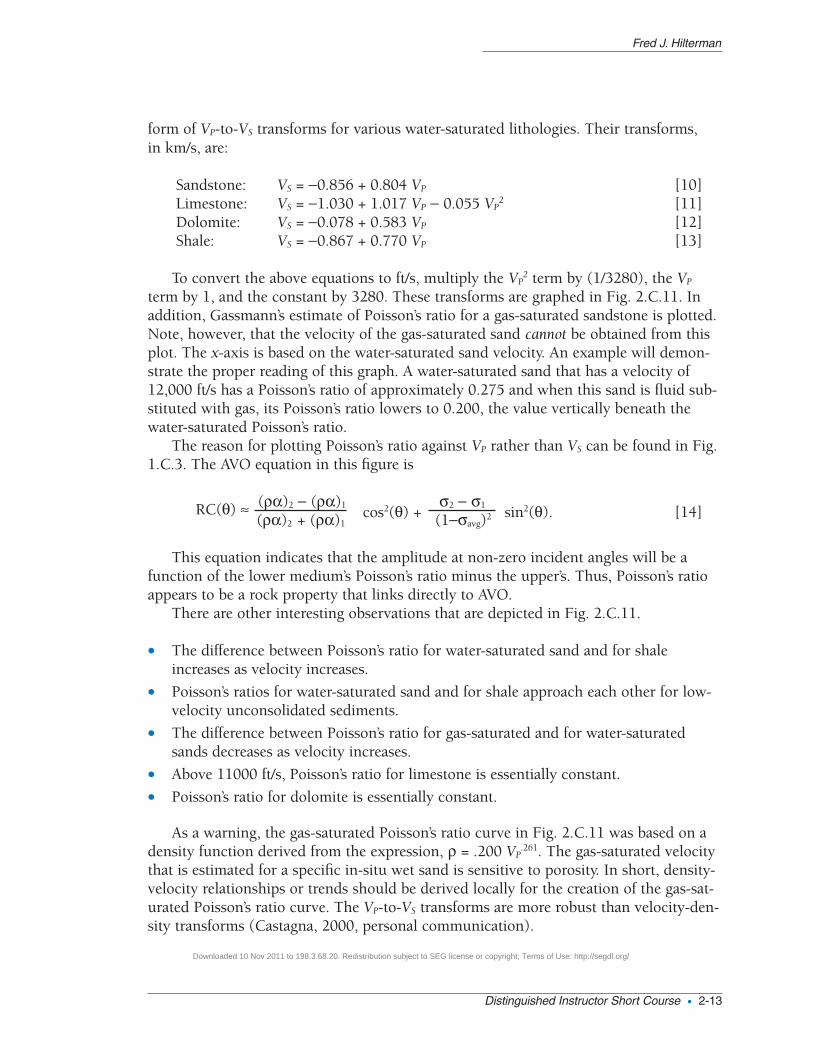
form of VP-to-VS transforms for various water-saturated lithologies. Their transforms, in km/s, are:
Sandstone: VS = −0.856 + 0.804 VP [10]Limestone: VS = −1.030 + 1.017 VP − 0.055 VP
2 [11]Dolomite: VS = −0.078 + 0.583 VP [12]Shale: VS = −0.867 + 0.770 VP [13]
To convert the above equations to ft/s, multiply the VP2 term by (1/3280), the VP
term by 1, and the constant by 3280. These transforms are graphed in Fig. 2.C.11. Inaddition, Gassmann’s estimate of Poisson’s ratio for a gas-saturated sandstone is plotted.Note, however, that the velocity of the gas-saturated sand cannot be obtained from thisplot. The x-axis is based on the water-saturated sand velocity. An example will demon-strate the proper reading of this graph. A water-saturated sand that has a velocity of12,000 ft/s has a Poisson’s ratio of approximately 0.275 and when this sand is fluid sub-stituted with gas, its Poisson’s ratio lowers to 0.200, the value vertically beneath thewater-saturated Poisson’s ratio.
The reason for plotting Poisson’s ratio against VP rather than VS can be found in Fig.1.C.3. The AVO equation in this figure is
RC(θ) ≈ (ρα)2 − (ρα)1 σ2 − σ1
(ρα)2 + (ρα)1cos2(θ) + (1−σavg)2 sin2(θ). [14]
This equation indicates that the amplitude at non-zero incident angles will be afunction of the lower medium’s Poisson’s ratio minus the upper’s. Thus, Poisson’s ratioappears to be a rock property that links directly to AVO.
There are other interesting observations that are depicted in Fig. 2.C.11.
• The difference between Poisson’s ratio for water-saturated sand and for shaleincreases as velocity increases.
• Poisson’s ratios for water-saturated sand and for shale approach each other for low-velocity unconsolidated sediments.
• The difference between Poisson’s ratio for gas-saturated and for water-saturatedsands decreases as velocity increases.
• Above 11000 ft/s, Poisson’s ratio for limestone is essentially constant.
• Poisson’s ratio for dolomite is essentially constant.
As a warning, the gas-saturated Poisson’s ratio curve in Fig. 2.C.11 was based on adensity function derived from the expression, ρ = .200 VP
.261. The gas-saturated velocitythat is estimated for a specific in-situ wet sand is sensitive to porosity. In short, density-velocity relationships or trends should be derived locally for the creation of the gas-sat-urated Poisson’s ratio curve. The VP-to-VS transforms are more robust than velocity-den-sity transforms (Castagna, 2000, personal communication).
Fred J. Hilterman
Distinguished Instructor Short Course • 2-13
04_Section 02_v2New.qxd 12/3/09 2:30 PM Page 2-13
Downloaded 10 Nov 2011 to 198.3.68.20. Redistribution subject to SEG license or copyright; Terms of Use: http://segdl.org/
2D. Relationships for Bulk Moduli
Just outside Golden, Colorado, the highway department has built a series of walkingpaths alongside a large road cut that traverses numerous outcropping formations. Anobserver will notice that within a particular formation, the rock properties vary signifi-cantly with respect to porosity, grain size, fracture patterns, rock types, etc. Any geo-physicist who has taken the time to view these outcrops has to marvel at the simplisticaveraging that is employed in the seismic method. Do we really assign just one velocityand one density to represent a formation’s properties? In essence, yes. Effective-mediumtheory is applied.
An effective medium is assumed to be macroscopically homogeneous and isotropic,so that only two elastic constants are necessary to define the entire medium or forma-tion. The key is to define an adequate mixing model of the composite material. Wangand Nur (1992) provide an excellent tutorial on the various petrophysical models andtheories that are commonly applied by geophysicists. In a sense, the Wyllie and R-H-Gtransforms are effective-medium theories that incorporate a mixing model in the choiceof Vma and Vfl.
But why are we examining effective-medium theories? One of the primary reasons isto estimate the changes in VP and VS for different pore-fluid saturants (Fig. 2. D.1). Thisprocess is often called fluid-replacement or fluid-substitution modeling. Most rocks arecomposed of at least two different materials: the matrix or grain material and the pore-fluid material. The example in the figure has two mineral components, quartz sand andshale. In addition, the pore fluid will have two components for the hydrocarbon state.
It was noted earlier that the velocities of the rock depend upon the bulk and shearmoduli of the total rock, along with the density. When the pore-fluid is changed in arock, the dry-rock bulk modulus (Kdry) and mineral bulk modulus (Kma) normallyremain the same. Only the fluid properties change. How does the total or effective mod-uli (K) of the rock change when only one component (pore-fluid) is changed? In orderto answer this question, methods to estimate Kma, Kdry and Kfl are needed.
In this section, I discuss several effective-medium theories that average the elasticconstants rather than the composite velocities of the medium. In addition, empiricalrelationships between the individual bulk moduli (Kma, Kdry and Kfl) will be examined.
Voigt, Reuss, and Hill’s (V-R-H) Moduli Models—Kma Estimate
In Fig. 2.D.2, VP and VS are expressed as a function of two effective moduli, Keff and µeff.These moduli represent the macroscopic scale of the material. In the late 1920s, Voigt(1928) and Reuss (1929) proposed two different mixing laws to compute these effectivemoduli from the individual moduli of the composite material. Reuss’s method providedthe lower limit for the effective moduli, while Voigt’s provided the upper limit. How-ever, Hill (1952) suggested that an average taken from the Voigt and Reuss modelswould yield a better estimate.
Wang and Nur (1992) tested the V-R-H model with laboratory data, and theirresults are shown in Fig. 2.D.3. As noted, the Voigt and Reuss models place upper andlower bounds on the effective moduli of the composite material. The Hill model comes
Seismic Amplitude Interpretation
2-14 • Society of Exploration Geophysicists / European Association of Geoscientists & Engineers
04_Section 02_v2New.qxd 12/3/09 2:30 PM Page 2-14
Downloaded 10 Nov 2011 to 198.3.68.20. Redistribution subject to SEG license or copyright; Terms of Use: http://segdl.org/
close to matching the best-fit curve for the bulk modulus, but the Hill model shouldnot be used to estimate the shear moduli. They also note that the V-R-H model shouldnot be used for gas-saturated rocks. These last two constraints limit the direct applica-tion of the V-R-H model for predicting VP and VS from a volumetric analysis of a rock.In short, the V-R-H model is used to estimate the effective bulk modulus of the mineral(grain) components, Kma, not the total bulk modulus.
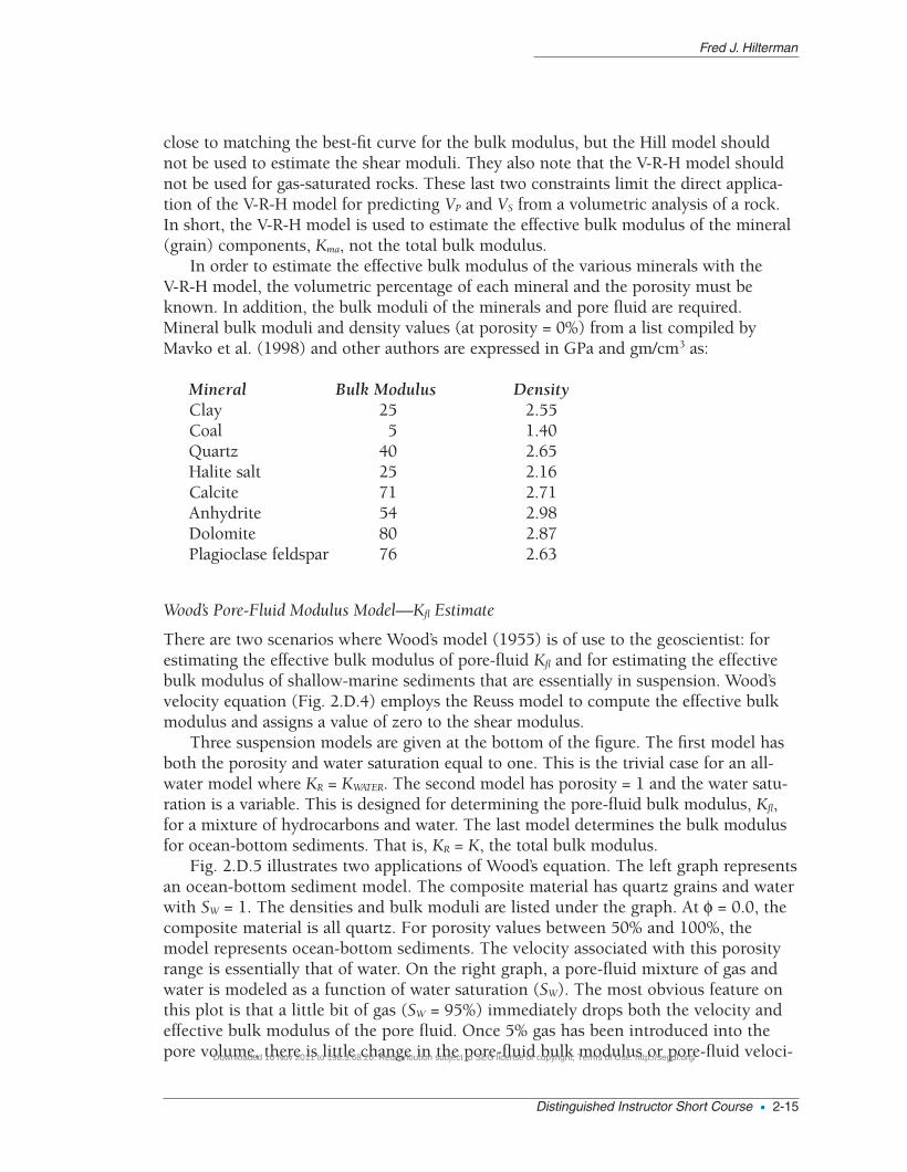
In order to estimate the effective bulk modulus of the various minerals with the V-R-H model, the volumetric percentage of each mineral and the porosity must beknown. In addition, the bulk moduli of the minerals and pore fluid are required.Mineral bulk moduli and density values (at porosity = 0%) from a list compiled byMavko et al. (1998) and other authors are expressed in GPa and gm/cm3 as:
Mineral Bulk Modulus DensityClay 25 2.55Coal 5 1.40Quartz 40 2.65Halite salt 25 2.16Calcite 71 2.71Anhydrite 54 2.98Dolomite 80 2.87Plagioclase feldspar 76 2.63
Wood’s Pore-Fluid Modulus Model—Kfl Estimate
There are two scenarios where Wood’s model (1955) is of use to the geoscientist: forestimating the effective bulk modulus of pore-fluid Kfl and for estimating the effectivebulk modulus of shallow-marine sediments that are essentially in suspension. Wood’svelocity equation (Fig. 2.D.4) employs the Reuss model to compute the effective bulkmodulus and assigns a value of zero to the shear modulus.
Three suspension models are given at the bottom of the figure. The first model hasboth the porosity and water saturation equal to one. This is the trivial case for an all-water model where KR = KWATER. The second model has porosity = 1 and the water satu-ration is a variable. This is designed for determining the pore-fluid bulk modulus, Kfl,for a mixture of hydrocarbons and water. The last model determines the bulk modulusfor ocean-bottom sediments. That is, KR = K, the total bulk modulus.
Fig. 2.D.5 illustrates two applications of Wood’s equation. The left graph representsan ocean-bottom sediment model. The composite material has quartz grains and waterwith SW = 1. The densities and bulk moduli are listed under the graph. At φ = 0.0, thecomposite material is all quartz. For porosity values between 50% and 100%, themodel represents ocean-bottom sediments. The velocity associated with this porosityrange is essentially that of water. On the right graph, a pore-fluid mixture of gas andwater is modeled as a function of water saturation (SW). The most obvious feature onthis plot is that a little bit of gas (SW = 95%) immediately drops both the velocity andeffective bulk modulus of the pore fluid. Once 5% gas has been introduced into thepore volume, there is little change in the pore-fluid bulk modulus or pore-fluid veloci-
Fred J. Hilterman
Distinguished Instructor Short Course • 2-15
04_Section 02_v2New.qxd 12/3/09 2:30 PM Page 2-15
Downloaded 10 Nov 2011 to 198.3.68.20. Redistribution subject to SEG license or copyright; Terms of Use: http://segdl.org/
ty. Obviously, this pore-fluid effect relates to the elastic properties of sands that havepartial gas saturation.
One difficulty with Wood’s model is that the shear modulus and thus VS areassumed to be zero. While the VP predicted from Wood’s model for shallow ocean-bot-tom sediments is fairly accurate when compared with actual field experiments, mea-sured VS is not zero. If VS were zero for suspended loads, then ocean-bottom horizontalphones would have difficulty recording converted PS waves. Hamilton (1979) publishedmeasured VS values for ocean-bottom (OB) sediments and his results indicate a changein the VS gradient at approximately 60 m beneath the ocean bottom. Marfurt (2000,personal communication) emphasized the importance of this VS gradient in separatingPP from PS wavefields in OB multicomponent data.
The effective pressure for shallow OB sediments is also akin to highly overpressuredsediments. Here, pore pressure approaches the overburden pressure (small effectivepressure) and the P-wave velocity decreases but the S-wave velocity decreases more dra-matically: same as with shallow OB sediments. This rapid decrease in VS was empha-sized to the author while examining an unpublished walkaway VSP. The PP waves fromthe VSP were very poor for detailing structure beneath the onset of abnormal pressure.However, the converted PS waves clearly imaged the reservoir and fault planes.
Batzle and Wang’s Estimation of Pore-Fluid Properties
In order to apply Wood’s equation for estimating the bulk modulus of the pore fluid,the bulk moduli of water and hydrocarbons are required. The values listed at the bot-tom of Fig. 2.D.5 were taken from Domenico’s (1974) graphs shown in Fig. 2.D.6 for adepth of 5000 ft (1500 m). While the density and bulk-moduli curves for oil and brineappear to be near one another in Figure 2.D.6, an increase in the gas-oil ratio will movethe oil curves quickly toward methane values.
A more detailed and recommended approach for determining the pore-fluid bulkmoduli and density has been given by Batzle and Wang (1992). Current pore-fluidmodeling programs implement some version of their algorithms. In their procedure, thebulk moduli and density of a pore-fluid component are expressed in terms of pore tem-perature, pressure, salinity, GOR, API number, and specific gas gravity. After the bulkmoduli of the pore-fluid components are determined, the effective bulk modulus of thetotal fluid is determined using Wood’s equation.
Biot’s Coefficient
In Fig. 2.A.2, the bulk modulus of the total rock K (effective rock bulk modulus)was shown to be dependent on three bulk moduli: the pore-fluid bulk modulus, Kfl;the matrix bulk modulus, Kma; and, the dry-rock bulk modulus, Kdry. As has been dis-cussed, two of these bulk moduli, Kfl and Kma, can be estimated if the volumetric min-eral and pore-fluid components of the rock are known. The third, Kdry, is elusive andyet, is a very important component for validating amplitude interpretations and pro-viding sensitivity analyses (the what-ifs). Thus, numerous petrophysicists have devel-oped empirical approximations to estimate this property based on other known prop-
Seismic Amplitude Interpretation
2-16 • Society of Exploration Geophysicists / European Association of Geoscientists & Engineers
04_Section 02_v2New.qxd 12/3/09 2:30 PM Page 2-16
Downloaded 10 Nov 2011 to 198.3.68.20. Redistribution subject to SEG license or copyright; Terms of Use: http://segdl.org/
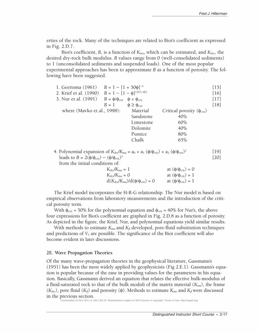
erties of the rock. Many of the techniques are related to Biot’s coefficient as expressedin Fig. 2.D.7.
Biot’s coefficient, B, is a function of Kma, which can be estimated, and Kdry, thedesired dry-rock bulk modulus. B values range from 0 (well-consolidated sediments)to 1 (unconsolidated sediments and suspended loads). One of the most popularexperimental approaches has been to approximate B as a function of porosity. The fol-lowing have been suggested.
1. Geertsma (1961) B = 1 − [1 + 50φ]−1 [15]2. Krief et al. (1990) B = 1 − [1 − φ][3/(1−φ)] [16]3. Nur et al. (1991) B = φ/φcrit φ < φcrit [17]
B = 1 φ ≥ φcrit [18]where (Mavko et al., 1998): Material Critical porosity (φcrit)
Sandstone 40%Limestone 60%Dolomite 40%Pumice 80%Chalk 65%
4. Polynomial expansion of Kdry/Kma = a0 + a1 (φ/φcrit) + a2 (φ/φcrit)2 [19]leads to B = 2(φ/φcrit) − (φ/φcrit)2 [20]from the initial conditions of:
Kdry/Kma = 1 at (φ/φcrit) = 0Kdry/Kma = 0 at (φ/φcrit) = 1d(Kdry/Kma)/d(φ/φcrit) = 0 at (φ/φcrit) = 1
The Krief model incorporates the H-R-G relationship. The Nur model is based onempirical observations from laboratory measurements and the introduction of the criti-cal porosity term.
With φcrit = 50% for the polynomial equation and φcrit = 40% for Nur’s, the abovefour expressions for Biot’s coefficient are graphed in Fig. 2.D.8 as a function of porosity.As depicted in the figure, the Krief, Nur, and polynomial equations yield similar results.
With methods to estimate Kma and Kfl developed, pore-fluid substitution techniquesand predictions of VS are possible. The significance of the Biot coefficient will alsobecome evident in later discussions.
2E. Wave Propagation Theories
Of the many wave-propagation theories in the geophysical literature, Gassmann’s(1951) has been the most widely applied by geophysicists (Fig 2.E.1). Gassmann’s equa-tion is popular because of the ease in providing values for the parameters in his equa-tion. Basically, Gassmann derived an equation that relates the effective bulk-modulus ofa fluid-saturated rock to that of the bulk moduli of the matrix material (Kma), the frame(Kdry), pore fluid (Kfl) and porosity (φ). Methods to estimate Kma and Kfl were discussedin the previous section.
Fred J. Hilterman
Distinguished Instructor Short Course • 2-17
04_Section 02_v2New.qxd 12/3/09 2:30 PM Page 2-17
Downloaded 10 Nov 2011 to 198.3.68.20. Redistribution subject to SEG license or copyright; Terms of Use: http://segdl.org/
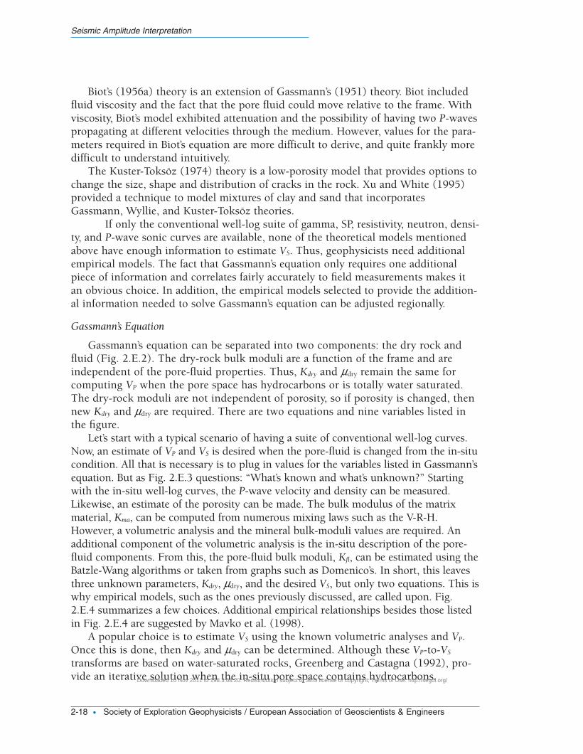
Biot’s (1956a) theory is an extension of Gassmann’s (1951) theory. Biot includedfluid viscosity and the fact that the pore fluid could move relative to the frame. Withviscosity, Biot’s model exhibited attenuation and the possibility of having two P-wavespropagating at different velocities through the medium. However, values for the para-meters required in Biot’s equation are more difficult to derive, and quite frankly moredifficult to understand intuitively.
The Kuster-Toksöz (1974) theory is a low-porosity model that provides options tochange the size, shape and distribution of cracks in the rock. Xu and White (1995)provided a technique to model mixtures of clay and sand that incorporatesGassmann, Wyllie, and Kuster-Toksöz theories.
If only the conventional well-log suite of gamma, SP, resistivity, neutron, densi-ty, and P-wave sonic curves are available, none of the theoretical models mentionedabove have enough information to estimate VS. Thus, geophysicists need additionalempirical models. The fact that Gassmann’s equation only requires one additionalpiece of information and correlates fairly accurately to field measurements makes itan obvious choice. In addition, the empirical models selected to provide the addition-al information needed to solve Gassmann’s equation can be adjusted regionally.
Gassmann’s Equation
Gassmann’s equation can be separated into two components: the dry rock andfluid (Fig. 2.E.2). The dry-rock bulk moduli are a function of the frame and areindependent of the pore-fluid properties. Thus, Kdry and mdry remain the same forcomputing VP when the pore space has hydrocarbons or is totally water saturated.The dry-rock moduli are not independent of porosity, so if porosity is changed, thennew Kdry and mdry are required. There are two equations and nine variables listed inthe figure.
Let’s start with a typical scenario of having a suite of conventional well-log curves.Now, an estimate of VP and VS is desired when the pore-fluid is changed from the in-situcondition. All that is necessary is to plug in values for the variables listed in Gassmann’sequation. But as Fig. 2.E.3 questions: “What’s known and what’s unknown?” Startingwith the in-situ well-log curves, the P-wave velocity and density can be measured.Likewise, an estimate of the porosity can be made. The bulk modulus of the matrixmaterial, Kma, can be computed from numerous mixing laws such as the V-R-H.However, a volumetric analysis and the mineral bulk-moduli values are required. Anadditional component of the volumetric analysis is the in-situ description of the pore-fluid components. From this, the pore-fluid bulk moduli, Kfl, can be estimated using theBatzle-Wang algorithms or taken from graphs such as Domenico’s. In short, this leavesthree unknown parameters, Kdry, mdry, and the desired VS, but only two equations. This iswhy empirical models, such as the ones previously discussed, are called upon. Fig.2.E.4 summarizes a few choices. Additional empirical relationships besides those listedin Fig. 2.E.4 are suggested by Mavko et al. (1998).
A popular choice is to estimate VS using the known volumetric analyses and VP.Once this is done, then Kdry and mdry can be determined. Although these VP-to-VS
transforms are based on water-saturated rocks, Greenberg and Castagna (1992), pro-vide an iterative solution when the in-situ pore space contains hydrocarbons.
Seismic Amplitude Interpretation
2-18 • Society of Exploration Geophysicists / European Association of Geoscientists & Engineers
04_Section 02_v2New.qxd 12/3/09 2:30 PM Page 2-18
Downloaded 10 Nov 2011 to 198.3.68.20. Redistribution subject to SEG license or copyright; Terms of Use: http://segdl.org/
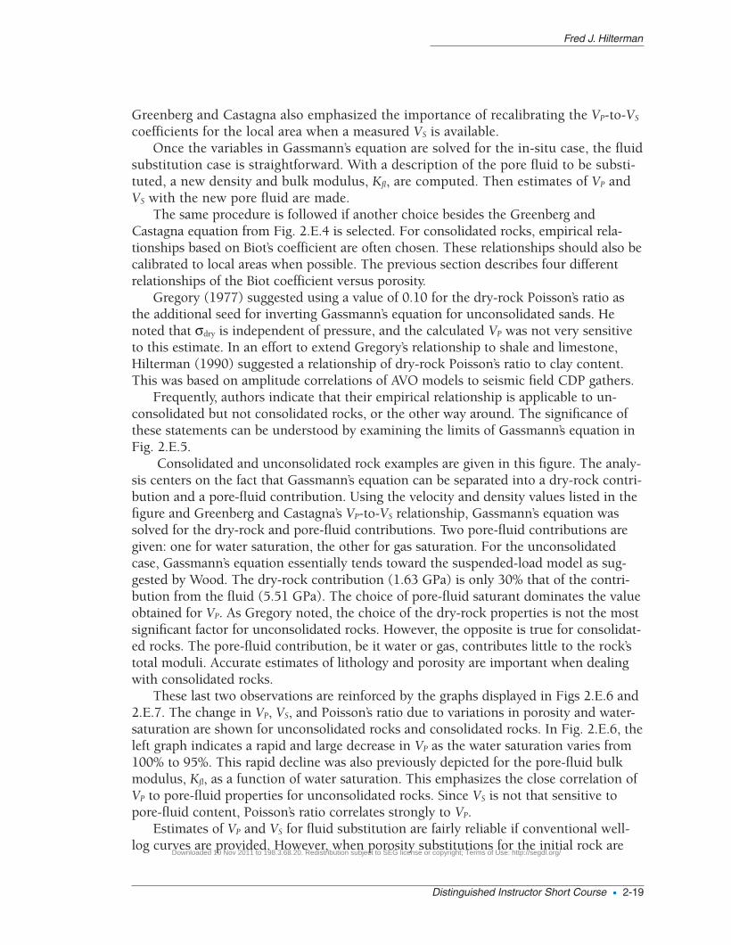
Greenberg and Castagna also emphasized the importance of recalibrating the VP-to-VS
coefficients for the local area when a measured VS is available. Once the variables in Gassmann’s equation are solved for the in-situ case, the fluid
substitution case is straightforward. With a description of the pore fluid to be substi-tuted, a new density and bulk modulus, Kfl, are computed. Then estimates of VP andVS with the new pore fluid are made.
The same procedure is followed if another choice besides the Greenberg andCastagna equation from Fig. 2.E.4 is selected. For consolidated rocks, empirical rela-tionships based on Biot’s coefficient are often chosen. These relationships should also becalibrated to local areas when possible. The previous section describes four differentrelationships of the Biot coefficient versus porosity.
Gregory (1977) suggested using a value of 0.10 for the dry-rock Poisson’s ratio asthe additional seed for inverting Gassmann’s equation for unconsolidated sands. Henoted that σdry is independent of pressure, and the calculated VP was not very sensitiveto this estimate. In an effort to extend Gregory’s relationship to shale and limestone,Hilterman (1990) suggested a relationship of dry-rock Poisson’s ratio to clay content.This was based on amplitude correlations of AVO models to seismic field CDP gathers.
Frequently, authors indicate that their empirical relationship is applicable to un-consolidated but not consolidated rocks, or the other way around. The significance ofthese statements can be understood by examining the limits of Gassmann’s equation inFig. 2.E.5.
Consolidated and unconsolidated rock examples are given in this figure. The analy-sis centers on the fact that Gassmann’s equation can be separated into a dry-rock contri-bution and a pore-fluid contribution. Using the velocity and density values listed in thefigure and Greenberg and Castagna’s VP-to-VS relationship, Gassmann’s equation wassolved for the dry-rock and pore-fluid contributions. Two pore-fluid contributions aregiven: one for water saturation, the other for gas saturation. For the unconsolidatedcase, Gassmann’s equation essentially tends toward the suspended-load model as sug-gested by Wood. The dry-rock contribution (1.63 GPa) is only 30% that of the contri-bution from the fluid (5.51 GPa). The choice of pore-fluid saturant dominates the valueobtained for VP. As Gregory noted, the choice of the dry-rock properties is not the mostsignificant factor for unconsolidated rocks. However, the opposite is true for consolidat-ed rocks. The pore-fluid contribution, be it water or gas, contributes little to the rock’stotal moduli. Accurate estimates of lithology and porosity are important when dealingwith consolidated rocks.
These last two observations are reinforced by the graphs displayed in Figs 2.E.6 and2.E.7. The change in VP, VS, and Poisson’s ratio due to variations in porosity and water-saturation are shown for unconsolidated rocks and consolidated rocks. In Fig. 2.E.6, theleft graph indicates a rapid and large decrease in VP as the water saturation varies from100% to 95%. This rapid decline was also previously depicted for the pore-fluid bulkmodulus, Kfl, as a function of water saturation. This emphasizes the close correlation ofVP to pore-fluid properties for unconsolidated rocks. Since VS is not that sensitive topore-fluid content, Poisson’s ratio correlates strongly to VP.
Estimates of VP and VS for fluid substitution are fairly reliable if conventional well-log curves are provided. However, when porosity substitutions for the initial rock are
Fred J. Hilterman
Distinguished Instructor Short Course • 2-19
04_Section 02_v2New.qxd 12/3/09 2:30 PM Page 2-19
Downloaded 10 Nov 2011 to 198.3.68.20. Redistribution subject to SEG license or copyright; Terms of Use: http://segdl.org/
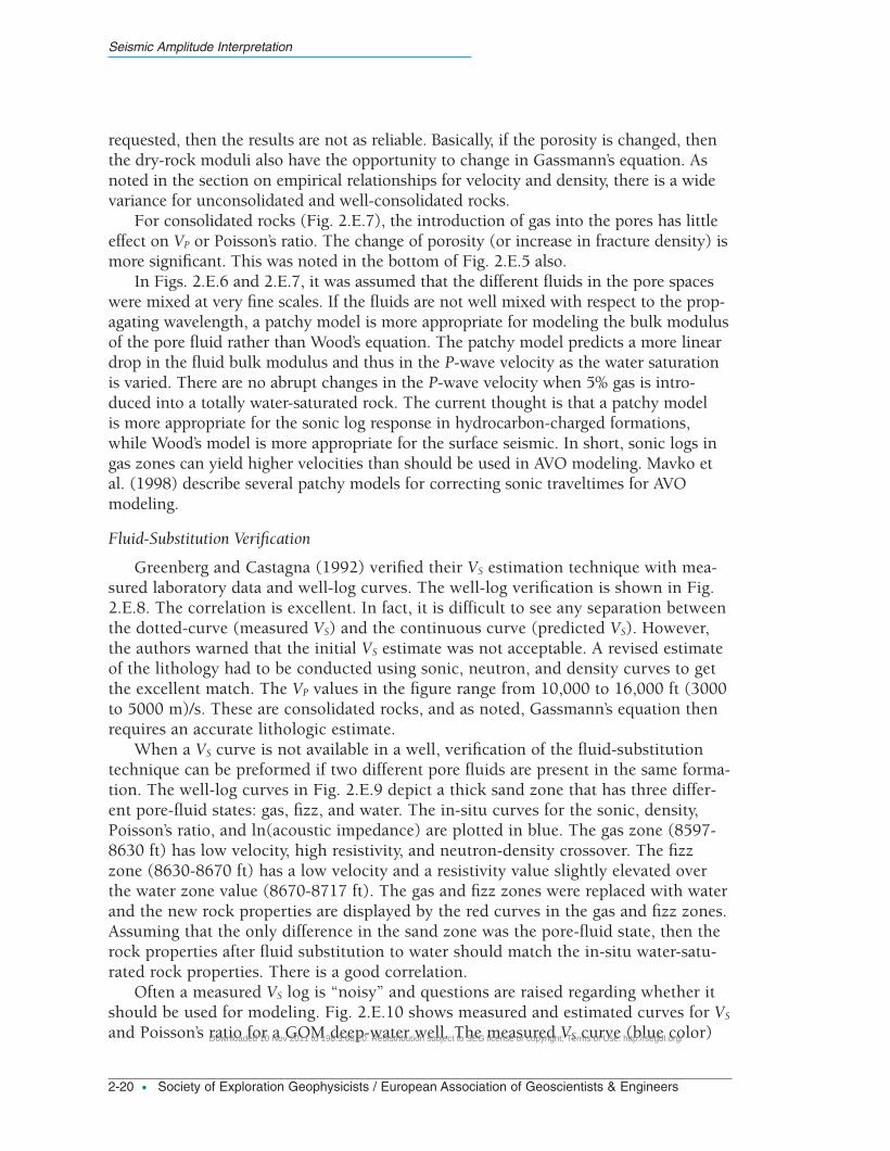
requested, then the results are not as reliable. Basically, if the porosity is changed, thenthe dry-rock moduli also have the opportunity to change in Gassmann’s equation. Asnoted in the section on empirical relationships for velocity and density, there is a widevariance for unconsolidated and well-consolidated rocks.
For consolidated rocks (Fig. 2.E.7), the introduction of gas into the pores has littleeffect on VP or Poisson’s ratio. The change of porosity (or increase in fracture density) ismore significant. This was noted in the bottom of Fig. 2.E.5 also.
In Figs. 2.E.6 and 2.E.7, it was assumed that the different fluids in the pore spaceswere mixed at very fine scales. If the fluids are not well mixed with respect to the prop-agating wavelength, a patchy model is more appropriate for modeling the bulk modulusof the pore fluid rather than Wood’s equation. The patchy model predicts a more lineardrop in the fluid bulk modulus and thus in the P-wave velocity as the water saturationis varied. There are no abrupt changes in the P-wave velocity when 5% gas is intro-duced into a totally water-saturated rock. The current thought is that a patchy model is more appropriate for the sonic log response in hydrocarbon-charged formations,while Wood’s model is more appropriate for the surface seismic. In short, sonic logs ingas zones can yield higher velocities than should be used in AVO modeling. Mavko etal. (1998) describe several patchy models for correcting sonic traveltimes for AVOmodeling.
Fluid-Substitution Verification
Greenberg and Castagna (1992) verified their VS estimation technique with mea-sured laboratory data and well-log curves. The well-log verification is shown in Fig.2.E.8. The correlation is excellent. In fact, it is difficult to see any separation betweenthe dotted-curve (measured VS) and the continuous curve (predicted VS). However,the authors warned that the initial VS estimate was not acceptable. A revised estimateof the lithology had to be conducted using sonic, neutron, and density curves to getthe excellent match. The VP values in the figure range from 10,000 to 16,000 ft (3000to 5000 m)/s. These are consolidated rocks, and as noted, Gassmann’s equation thenrequires an accurate lithologic estimate.
When a VS curve is not available in a well, verification of the fluid-substitutiontechnique can be preformed if two different pore fluids are present in the same forma-tion. The well-log curves in Fig. 2.E.9 depict a thick sand zone that has three differ-ent pore-fluid states: gas, fizz, and water. The in-situ curves for the sonic, density,Poisson’s ratio, and ln(acoustic impedance) are plotted in blue. The gas zone (8597-8630 ft) has low velocity, high resistivity, and neutron-density crossover. The fizzzone (8630-8670 ft) has a low velocity and a resistivity value slightly elevated overthe water zone value (8670-8717 ft). The gas and fizz zones were replaced with waterand the new rock properties are displayed by the red curves in the gas and fizz zones.Assuming that the only difference in the sand zone was the pore-fluid state, then therock properties after fluid substitution to water should match the in-situ water-satu-rated rock properties. There is a good correlation.
Often a measured VS log is “noisy” and questions are raised regarding whether itshould be used for modeling. Fig. 2.E.10 shows measured and estimated curves for VS
and Poisson’s ratio for a GOM deep-water well. The measured VS curve (blue color)
Seismic Amplitude Interpretation
2-20 • Society of Exploration Geophysicists / European Association of Geoscientists & Engineers
04_Section 02_v2New.qxd 12/3/09 2:30 PM Page 2-20
Downloaded 10 Nov 2011 to 198.3.68.20. Redistribution subject to SEG license or copyright; Terms of Use: http://segdl.org/
has high-frequency variations that are not present on the other logs. The extreme val-ues for these VS fluctuations do not appear to be real. In situations such as this, the“good” zones of the measured VS curve can be used to develop new regression coeffi-cients for VP-to-VS transforms and then the estimated VS is used for AVO modeling(Chesser, 1997).
Summary—Example of Fluid-Substitution Modeling
Numerous empirical and theoretical models have been described up to this point andthe average reader should be swamped with thoughts such as “When to apply what.”An example of a typical fluid substitution for AVO modeling should answer some ofthese questions.
Let’s assume that a prospect has been defined near a well that has conventional well-log curves. Migrated CDP gathers have been obtained near the well and an AVO synthet-ic is desired to compare to the gathers. The well doesn’t have hydrocarbons and an AVOsynthetic is also desired to determine the seismic signature when various pore fluids aresubstituted for the in-situ brine. The petrophysical problem is to determine VS for the in-situ AVO modeling and VP, VS, and ρ for the fluid-replacement AVO modeling.
The VS prediction for the water-saturated in-situ rocks is simple, as illustrated inFig. 2.E.11. The subscripts [,WET] and [,GAS] on the rock-property variables refer tothe water-saturated and hydrocarbon-saturated states, respectively. Using the litholog-ic curves, the volume of each mineral component is determined at each depth point.The example rock is composed of 85% sand and 15% shale with an in-situ velocity of11,400 ft (3500 m)/s. The simplest method of predicting VS is by VP-to-VS transforms,such as those published by Greenberg and Castagna (1992). Once VS is determinedfor the shale and sand components, the component velocities are averaged using theVoigt-Reuss-Hill effective-medium model. This procedure is repeated for the entiredepth of the well. With VP and density values taken from the in-situ logs and VS pre-dicted as shown, the in-situ AVO synthetic can now be generated.
The petrophysical work needed for fluid-substitution AVO modeling is covered inthe next four figures. As shown in the upper portion of Fig. 2.E.12, porosity and den-sity are additional parameters required for pore-fluid substitution. Of course, thedesired SW and the pore-fluid description (API, GOR, etc.) need to be defined.
The solution is broken into two parts. In the first part, (A), the elastic constantsfor the water-saturated rock are estimated and then these elastic constants are used inthe second part (B) when new pore fluids are introduced. In Fig. 2.E.12, model equa-tions and numeric values for estimating the bulk moduli of the total rock (KWET), porefluid (Kfl,WET), and minerals (Kma) are given. For convenience in this example, the den-sity and modulus for the pore fluid were taken from Domenico’s table. However, it isrecommended that Batzle-Wang’s method of estimating the pore-fluid properties befollowed. Domenico’s values were derived for a specific set of environmental condi-tions (pressure and temperature gradients, specific gas density, salinity, etc.) and theseconditions would normally not match other areas. Mavko et al. (1998) provided step-by-step numeric examples for calculating the pore-fluid properties with the Batzle-Wang equations.
Fred J. Hilterman
Distinguished Instructor Short Course • 2-21
04_Section 02_v2New.qxd 12/3/09 2:30 PM Page 2-21
Downloaded 10 Nov 2011 to 198.3.68.20. Redistribution subject to SEG license or copyright; Terms of Use: http://segdl.org/
The next step, shown in Fig. 2.E.13, contains the Greenberg-Castagna inversion ofGassmann’s equation to find Kdry. The X, Y, and b shown in Part A.3 have no physicalmeaning; they are only intermediate variables to aid in the solution.
This is not the only technique for estimating Kdry. In Fig. 2.E.4, two other methodsfor obtaining Kdry were suggested. One is the Biot coefficient technique. If Biot’s coeffi-cient is approximated with one of the models described in Fig. 2.D.8, then Kdry = (1−B)Kma. Remember B is based on the known porosity and Kma has been determined in theprevious figure. Now, the only variable that is unknown in Gassmann’s equation for VP
is µdry. Once this is found, the new pore fluids can be introduced (following step A.4 inFig. 2.E.13).
The other method suggested in Fig. 2.E.4 for estimating Kdry is to use the dry-rockPoisson’s ratio. If this model is selected for providing additional information toGassmann’s equation, then a solution proposed by Gregory (1977) can be employed.Application of any of these three methods (Greenberg-Castagna, Biot’s coefficient, ordry-rock Poisson’s ratio) will supply the information listed in Fig. 2.E.13 at the end ofPart A.3. The last portion for estimating the properties of the water-saturated rock isgiven in Part A.4 of Fig. 2.E.13.
The last petrophysical stage for AVO modeling with fluid-substitution properties israther straightforward. The only additional rock properties needed, beyond what wascalculated from the water-saturated case, are the hydrocarbon-charged values for thetotal rock density and the pore-fluid bulk modulus. Then the rock properties associatedwith the hydrocarbon-charged state are inserted into Gassmann’s equation. These stepsare worked out with numeric values in Figs. 2.E.14 and 2.E.15.
2F. Back to Geology through Anstey
With all the theoretical and empirical relationships presented in this section, theauthor seems to have lost sight of geologic processes. How does one return to thebasics? There is no better way than through the geophysicist’s own Shakespeareanorator, Nigel Anstey. All geophysicists who have made Society presentations and alsolistened to one of Nigel’s inspiring presentations develop a fear for the future. Thatfear is, “Oh Lord, please never make me follow Nigel in a technical presentation!”
Nigel gave such an illuminating presentation at Cambridge in 1990 that it wasreproduced in First Break. After a few cartoons on squeezing and distorting the shapeof a rock, it became obvious that a grain’s shape and the number of contacts it haswith other grains were going to be an important factor in predicting the S-wave veloc-ity of the rock. Several of his intuitive observations are summarized in Fig. 2.F.1. Hisconclusions of the factors that control S-wave velocity were:
• First and foremost [is], probably, the cementation. Advanced cementationmakes all rocks look much the same.
• But if there is no cementation, then [there are] those factors that control thenumber and angularity of the grain contacts—shape, then sorting, then over-burden pressure.
Seismic Amplitude Interpretation
2-22 • Society of Exploration Geophysicists / European Association of Geoscientists & Engineers
04_Section 02_v2New.qxd 12/3/09 2:30 PM Page 2-22
Downloaded 10 Nov 2011 to 198.3.68.20. Redistribution subject to SEG license or copyright; Terms of Use: http://segdl.org/
• Now—where’s lithology? Well, we will list it; the intrinsic rigidity of the grainmaterial must be there, as must that of the cement. But not very clearly—part-ly because different lithologies often imply different angularity of the graincontacts, different natural cements, different susceptibility to pressure solu-tion, different susceptibility to fracture, and so on ... [and] partly because thelithology becomes less important at porosities of reservoir quality.
• Then [there is] clay content—ranging from the low side of modest if the clayparticles are just passengers in the pores, to the high side of modest if they areactually in the contacts. Then [there is] the saturant (just the minor effect ofdensity), and the grain size (insofar as it controls the closing effect of over-burden pressure, and preferential cementation).
Also noted was that porosity, as such, is not a major control on S-wave velocity. But Nigel also wanted his conclusions to be phrased in terms that geologists know
and understand, and this is accomplished as shown in the Fig. 2.F.2. The emphasis isthat the number of grain contacts affects the rigidity of the rock. For fine-grainedrocks, cement is likely to form preferentially in small pores and thus the rocks willhave a higher rigidity than do coarse-grained rocks. Coarse-grained rocks that arewell-rounded and well-sorted have fairly good porosity, and have many rigid contactsand thus a high shear-wave velocity for that porosity. This relates to the previous dis-cussion on Han’s observation of very-clean sand specimens. For angular-grainedrocks, the sorting and packing, which can be related to geologic processes, control thenumber of contacts and thus the S-wave velocity.
While Anstey wanted to emphasize that examination of thin sections will provideinsight into the geologic processes and thus predictions about the S-wave velocity,one has to wonder if these same predictions can be made from an interpretationbased on seismic sequence stratigraphy.
Fred J. Hilterman
Distinguished Instructor Short Course • 2-23
04_Section 02_v2New.qxd 12/3/09 2:30 PM Page 2-23
Downloaded 10 Nov 2011 to 198.3.68.20. Redistribution subject to SEG license or copyright; Terms of Use: http://segdl.org/
Seismic Amplitude Interpretation
2-24 • Society of Exploration Geophysicists / European Association of Geoscientists & Engineers
Figures
Figure 2.A.1
Figure 2.A.2
Figure 2.A.3
04_Section 02_v2New.qxd 12/3/09 2:30 PM Page 2-24
Downloaded 10 Nov 2011 to 198.3.68.20. Redistribution subject to SEG license or copyright; Terms of Use: http://segdl.org/
Fred J. Hilterman
Distinguished Instructor Short Course • 2-25
Figure 2.A.4
Figure 2.A.5
04_Section 02_v2New.qxd 12/3/09 2:30 PM Page 2-25
Downloaded 10 Nov 2011 to 198.3.68.20. Redistribution subject to SEG license or copyright; Terms of Use: http://segdl.org/
Seismic Amplitude Interpretation
2-26 • Society of Exploration Geophysicists / European Association of Geoscientists & Engineers
Figure 2.A.6
Figure 2.B.1
04_Section 02_v2New.qxd 12/3/09 2:30 PM Page 2-26
Downloaded 10 Nov 2011 to 198.3.68.20. Redistribution subject to SEG license or copyright; Terms of Use: http://segdl.org/
Fred J. Hilterman
Distinguished Instructor Short Course • 2-27
Figure 2.B.2
Figure 2.B.3
Figure 2.B.4
04_Section 02_v2New.qxd 12/3/09 2:30 PM Page 2-27
Downloaded 10 Nov 2011 to 198.3.68.20. Redistribution subject to SEG license or copyright; Terms of Use: http://segdl.org/
Seismic Amplitude Interpretation
2-28 • Society of Exploration Geophysicists / European Association of Geoscientists & Engineers
Figure 2.B.5
Figure 2.B.6
Figure 2.B.7
04_Section 02_v2New.qxd 12/3/09 2:30 PM Page 2-28
Downloaded 10 Nov 2011 to 198.3.68.20. Redistribution subject to SEG license or copyright; Terms of Use: http://segdl.org/
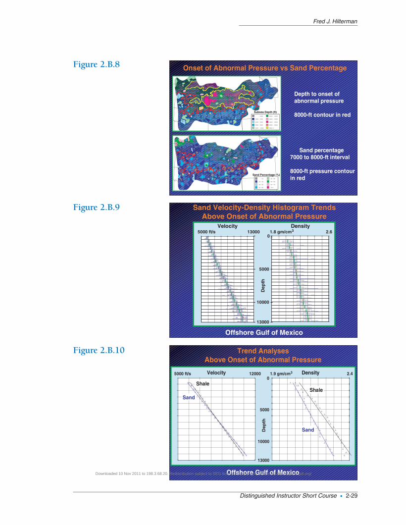
Fred J. Hilterman
Distinguished Instructor Short Course • 2-29
Figure 2.B.8
Figure 2.B.9
Figure 2.B.10
1
Onset of Abnormal Pressure vs Sand Percentage
Subsea Depth (feet)
- 2 0 0 0 1 0 0 0 0 - 1 2 0 0 0
2 0 0 0 - 4 0 0 0 1 2 0 0 0 - 1 4 0 0 0
4 0 0 0 - 6 0 0 0 1 4 0 0 0 - 1 6 0 0 0
6 0 0 0 - 8 0 0 0 1 6 0 0 0 - 1 8 0 0 0
8 0 0 0 - 1 0 0 0 0 1 8 0 0 0 +
Sand Percentage (%)
- 10 40 - 50
10 - 20 50 - 60
20 - 30 60 - 70
30 - 40 70 +
Depth to onset ofabnormal pressure
8000-ft contour in red
Sand percentage7000 to 8000-ft interval
8000-ft pressure contourin red
- 2000 10000 - 12000
2000 - 4000 12000 - 14000
4000 - 6000 14000 - 16000
6000 - 8000 16000 - 18000
8000 - 10000 18000 +
- 10 40 - 50
10 - 20 50 - 60
20 - 30 60 - 70
30 - 40 70 +
Subsea Depth (ft)
Sand Percentage (%)
04_Section 02_v2New.qxd 12/3/09 2:31 PM Page 2-29
Downloaded 10 Nov 2011 to 198.3.68.20. Redistribution subject to SEG license or copyright; Terms of Use: http://segdl.org/
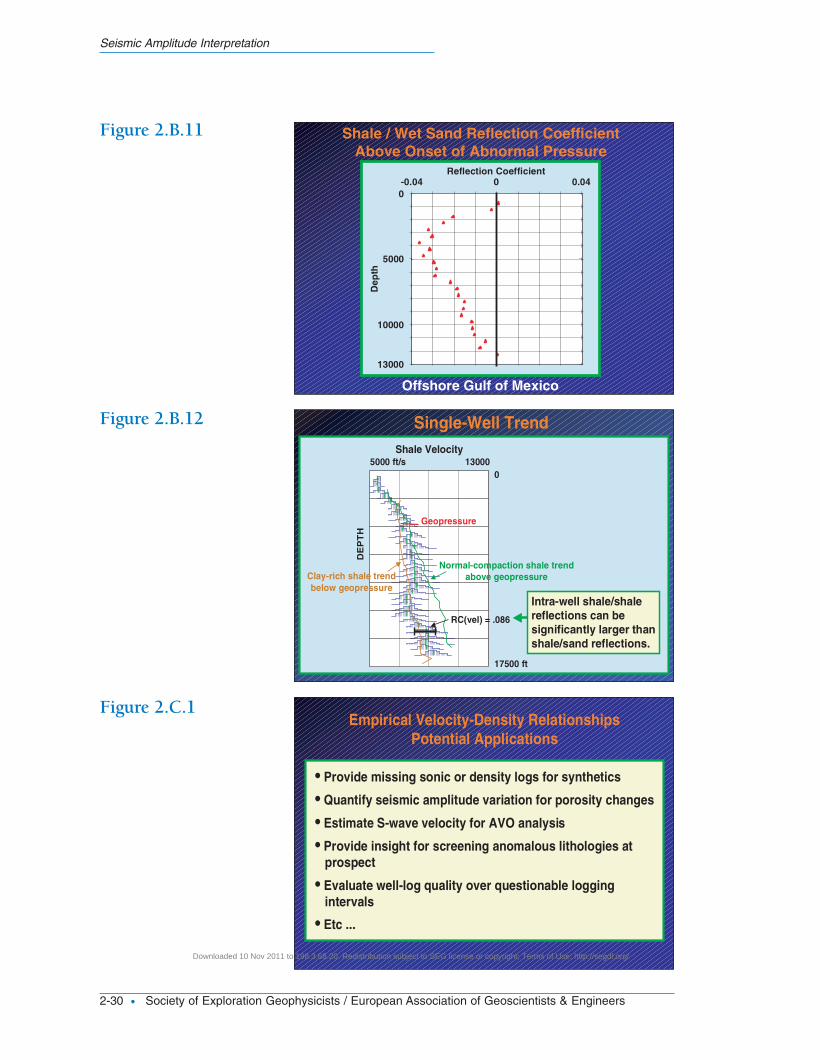
Seismic Amplitude Interpretation
2-30 • Society of Exploration Geophysicists / European Association of Geoscientists & Engineers
Figure 2.B.11
Figure 2.B.12
Figure 2.C.1
04_Section 02_v2New.qxd 12/3/09 2:31 PM Page 2-30
Downloaded 10 Nov 2011 to 198.3.68.20. Redistribution subject to SEG license or copyright; Terms of Use: http://segdl.org/
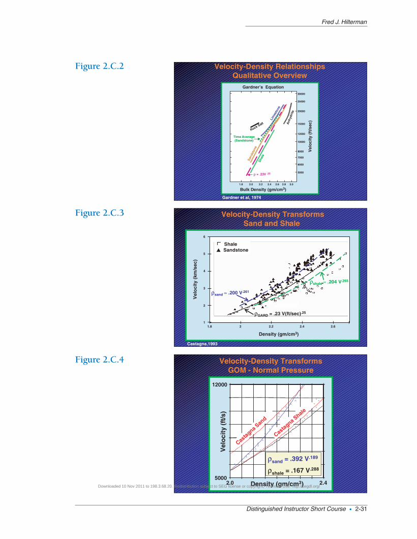
Fred J. Hilterman
Distinguished Instructor Short Course • 2-31
Figure 2.C.2
Figure 2.C.3
Figure 2.C.4
04_Section 02_v2New.qxd 12/3/09 2:31 PM Page 2-31
Downloaded 10 Nov 2011 to 198.3.68.20. Redistribution subject to SEG license or copyright; Terms of Use: http://segdl.org/
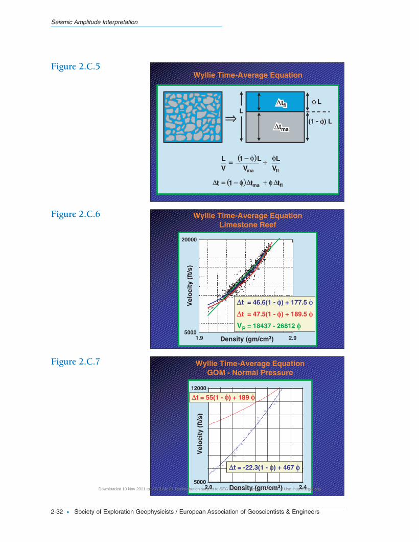
Seismic Amplitude Interpretation
2-32 • Society of Exploration Geophysicists / European Association of Geoscientists & Engineers
Figure 2.C.5
Figure 2.C.6
Figure 2.C.7
04_Section 02_v2New.qxd 12/3/09 2:31 PM Page 2-32
Downloaded 10 Nov 2011 to 198.3.68.20. Redistribution subject to SEG license or copyright; Terms of Use: http://segdl.org/
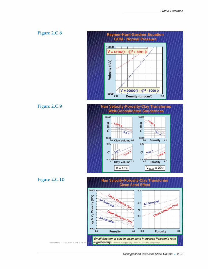
Fred J. Hilterman
Distinguished Instructor Short Course • 2-33
Figure 2.C.8
Figure 2.C.9
Figure 2.C.10
04_Section 02_v2New.qxd 12/3/09 2:31 PM Page 2-33
Downloaded 10 Nov 2011 to 198.3.68.20. Redistribution subject to SEG license or copyright; Terms of Use: http://segdl.org/
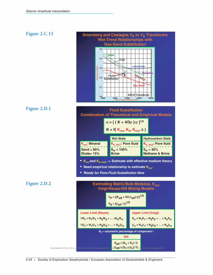
Seismic Amplitude Interpretation
2-34 • Society of Exploration Geophysicists / European Association of Geoscientists & Engineers
Figure 2.C.11
Figure 2.D.1
Figure 2.D.2
04_Section 02_v2New.qxd 12/3/09 2:31 PM Page 2-34
Downloaded 10 Nov 2011 to 198.3.68.20. Redistribution subject to SEG license or copyright; Terms of Use: http://segdl.org/
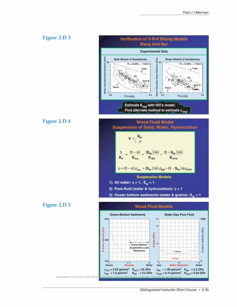
Fred J. Hilterman
Distinguished Instructor Short Course • 2-35
Figure 2.D.3
Figure 2.D.4
Figure 2.D.5
04_Section 02_v2New.qxd 12/3/09 2:31 PM Page 2-35
Downloaded 10 Nov 2011 to 198.3.68.20. Redistribution subject to SEG license or copyright; Terms of Use: http://segdl.org/
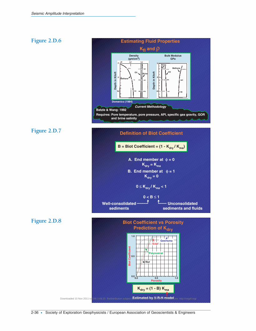
Seismic Amplitude Interpretation
2-36 • Society of Exploration Geophysicists / European Association of Geoscientists & Engineers
Figure 2.D.6
Figure 2.D.7
Figure 2.D.8
04_Section 02_v2New.qxd 12/3/09 2:31 PM Page 2-36
Downloaded 10 Nov 2011 to 198.3.68.20. Redistribution subject to SEG license or copyright; Terms of Use: http://segdl.org/
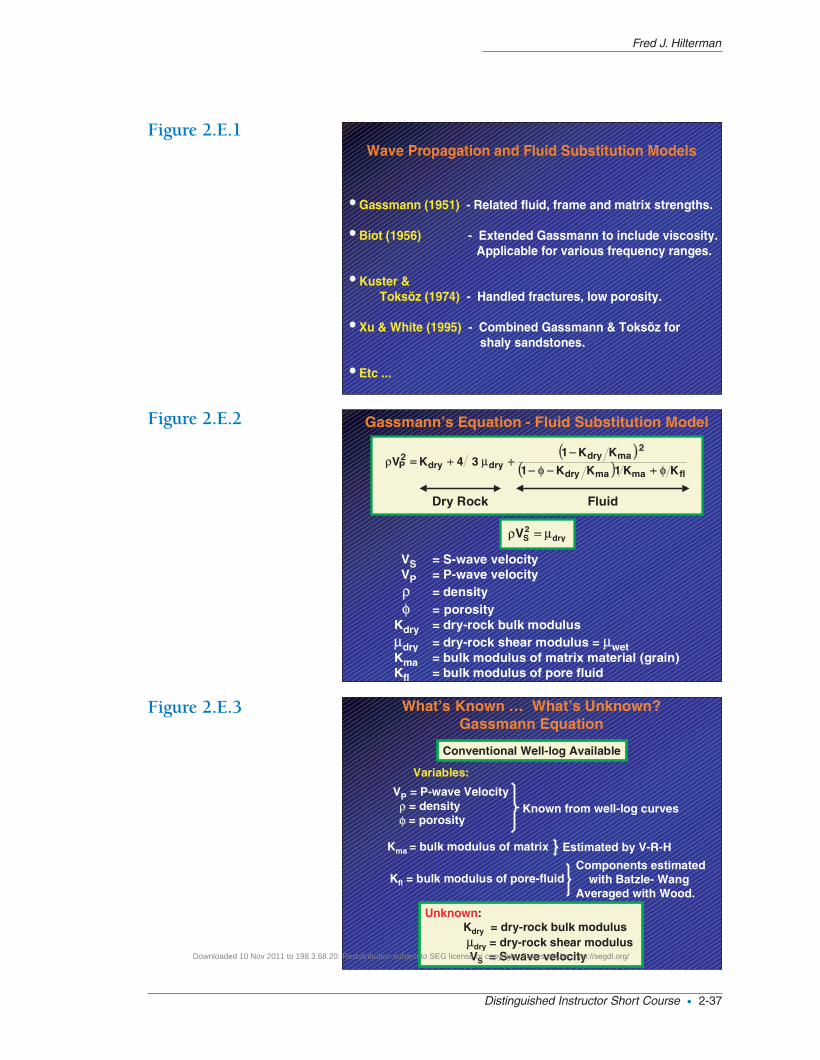
Fred J. Hilterman
Distinguished Instructor Short Course • 2-37
Figure 2.E.1
Figure 2.E.2
Figure 2.E.3
04_Section 02_v2New.qxd 12/3/09 2:31 PM Page 2-37
Downloaded 10 Nov 2011 to 198.3.68.20. Redistribution subject to SEG license or copyright; Terms of Use: http://segdl.org/
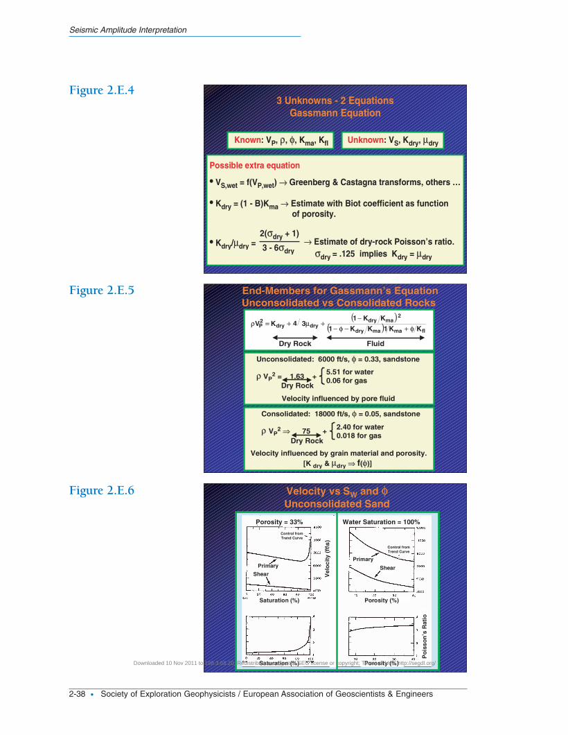
Seismic Amplitude Interpretation
2-38 • Society of Exploration Geophysicists / European Association of Geoscientists & Engineers
Figure 2.E.4
Figure 2.E.5
Figure 2.E.6
04_Section 02_v2New.qxd 12/3/09 2:31 PM Page 2-38
Downloaded 10 Nov 2011 to 198.3.68.20. Redistribution subject to SEG license or copyright; Terms of Use: http://segdl.org/
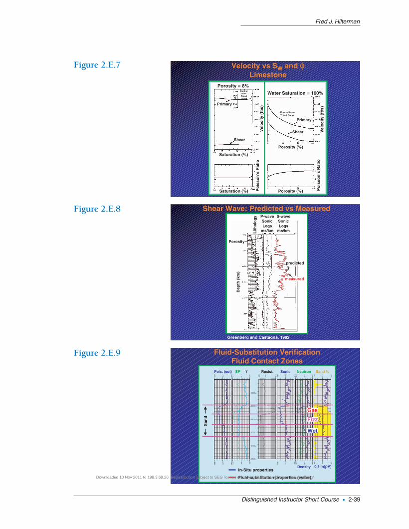
Fred J. Hilterman
Distinguished Instructor Short Course • 2-39
Figure 2.E.7
Figure 2.E.8
Figure 2.E.9
04_Section 02_v2New.qxd 12/3/09 2:31 PM Page 2-39
Downloaded 10 Nov 2011 to 198.3.68.20. Redistribution subject to SEG license or copyright; Terms of Use: http://segdl.org/
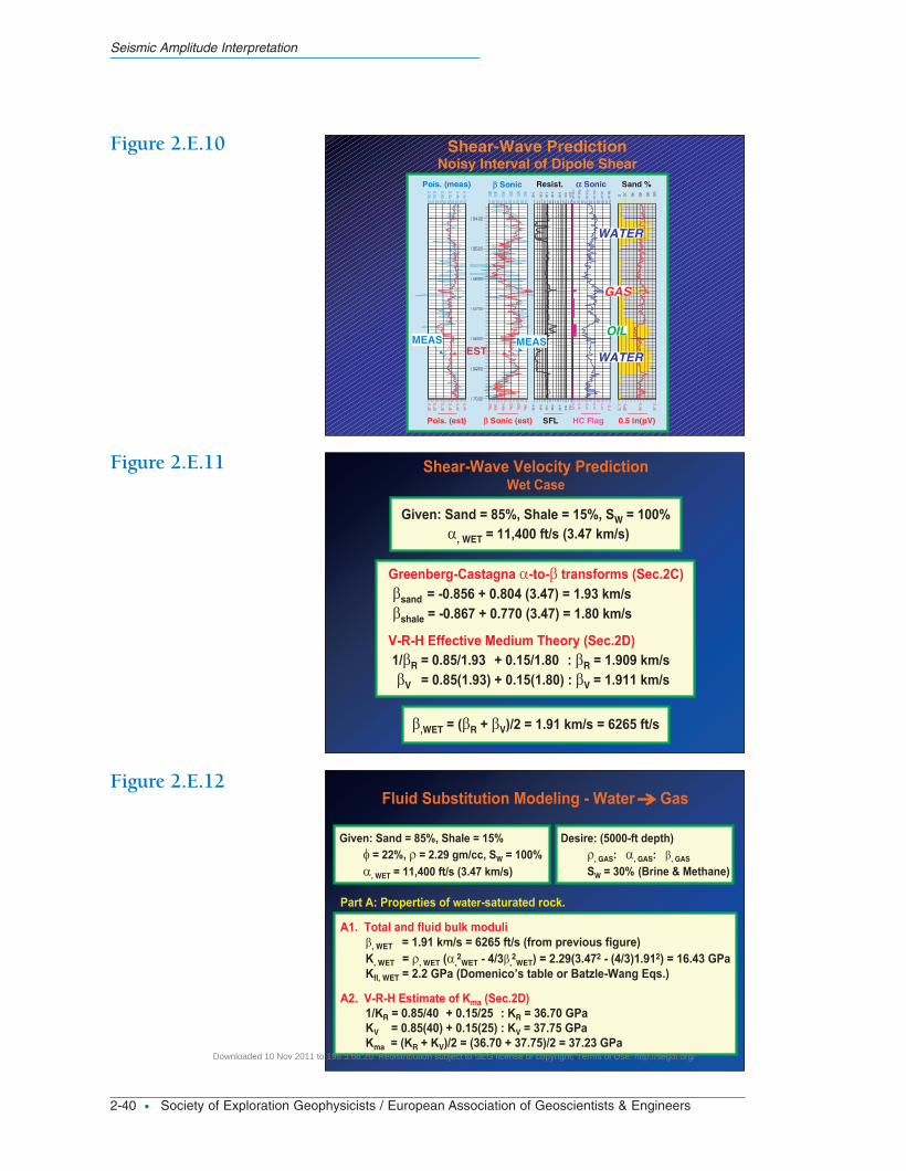
Seismic Amplitude Interpretation
2-40 • Society of Exploration Geophysicists / European Association of Geoscientists & Engineers
Figure 2.E.10
Figure 2.E.11
Figure 2.E.12
04_Section 02_v2New.qxd 12/3/09 2:31 PM Page 2-40
Downloaded 10 Nov 2011 to 198.3.68.20. Redistribution subject to SEG license or copyright; Terms of Use: http://segdl.org/
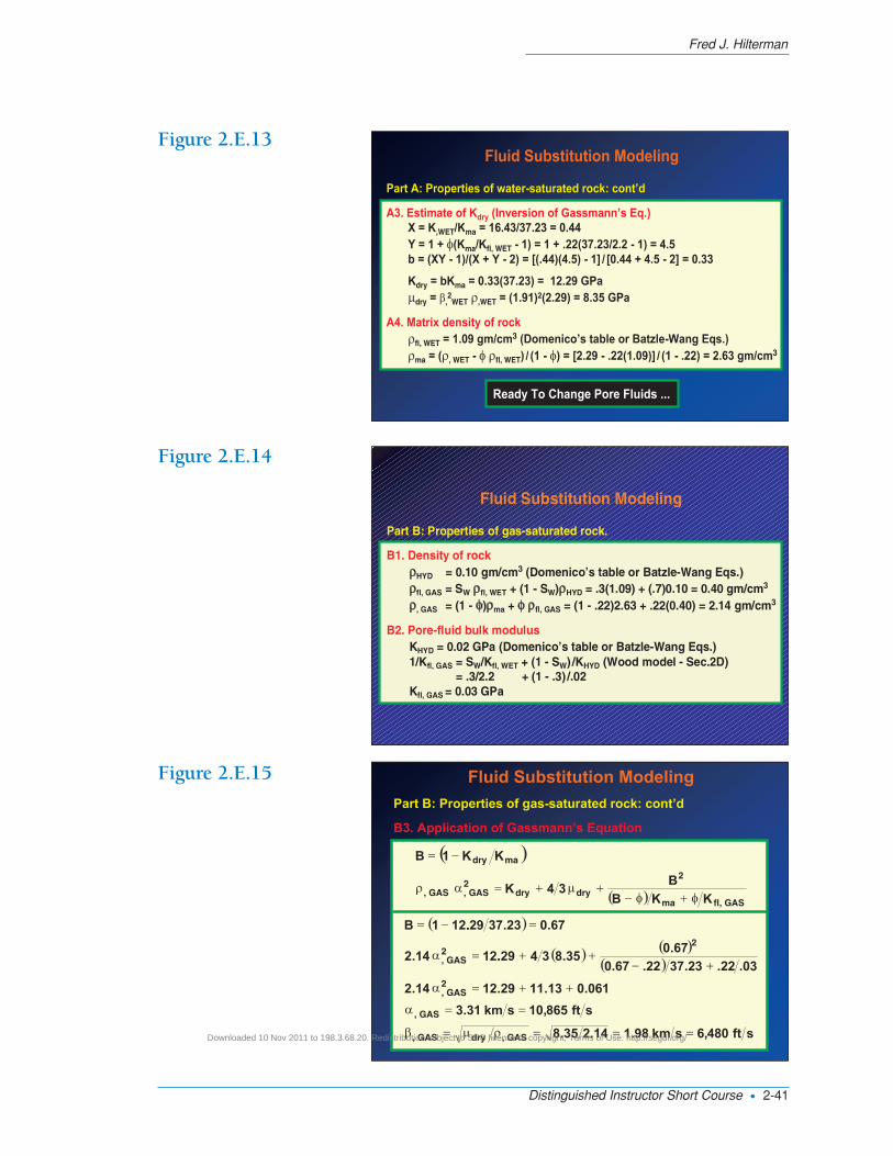
Fred J. Hilterman
Distinguished Instructor Short Course • 2-41
Figure 2.E.13
Figure 2.E.14
Figure 2.E.15
04_Section 02_v2.qxd 1/13/06 1:30 PM Page 2-41
Downloaded 10 Nov 2011 to 198.3.68.20. Redistribution subject to SEG license or copyright; Terms of Use: http://segdl.org/
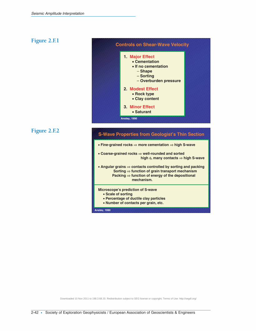
Seismic Amplitude Interpretation
2-42 • Society of Exploration Geophysicists / European Association of Geoscientists & Engineers
Figure 2.F.1
Figure 2.F.2
04_Section 02_v2New.qxd 12/3/09 2:31 PM Page 2-42
Downloaded 10 Nov 2011 to 198.3.68.20. Redistribution subject to SEG license or copyright; Terms of Use: http://segdl.org/