scalable fine-grained call path tracing
TRANSCRIPT
Scalable Fine-grained Call Path Tracing
Nathan R. TallentRice University
John Mellor-CrummeyRice University
[email protected] Franco
Rice [email protected]
Reed LandrumStanford University
Laksono AdhiantoRice University
ABSTRACTApplications must scale well to make efficient use of evenmedium-scale parallel systems. Because scaling problemsare often difficult to diagnose, there is a critical need forscalable tools that guide scientists to the root causes of per-formance bottlenecks.
Although tracing is a powerful performance-analysis tech-nique, tools that employ it can quickly become bottlenecksthemselves. Moreover, to obtain actionable performancefeedback for modular parallel software systems, it is of-ten necessary to collect and present fine-grained context-sensitive data — the very thing scalable tools avoid. Whileexisting tracing tools can collect calling contexts, they do soonly in a coarse-grained fashion; and no prior tool scalablypresents both context- and time-sensitive data.
This paper describes how to collect, analyze and presentfine-grained call path traces for parallel programs. To scaleour measurements, we use asynchronous sampling, whosegranularity is controlled by a sampling frequency, and a com-pact representation. To present traces at multiple levels ofabstraction and at arbitrary resolutions, we use samplingto render complementary slices of calling-context-sensitivetrace data. Because our techniques are general, they can beused on applications that use different parallel programmingmodels (MPI, OpenMP, PGAS). This work is implementedin HPCToolkit.
Categories and Subject DescriptorsC.4 [Performance of systems]: Measurement techniques,Performance attributes
General TermsAlgorithms, Measurement, Performance
Keywordstracing, calling context, statistical sampling, performancetools, HPCToolkit
Permission to make digital or hard copies of all or part of this work forpersonal or classroom use is granted without fee provided that copies arenot made or distributed for profit or commercial advantage and that copiesbear this notice and the full citation on the first page. To copy otherwise, torepublish, to post on servers or to redistribute to lists, requires prior specificpermission and/or a fee.ICS’11, May 31–June 4, 2011, Tuscon, Arizona, USA.Copyright 2011 ACM 978-1-4503-0102-2/11/05 ...$10.00.
1. INTRODUCTIONAs hardware-thread counts increase in supercomputers,
applications must scale to make effective use of computingresources. However, inefficiencies that do not even appearat smaller scales can become major bottlenecks at largerscales. Because scaling problems are often difficult to diag-nose, there is a critical need for tools that guide scientiststo the root causes of performance bottlenecks.
Tracing has long been a method of choice for many per-formance tools [6,8,9,12,15,17,19,22,24,30,31,33,35,43,44].Because performance traces show how a program’s behav-ior changes over time — or, more generally, with respect toa progress metric — tracing is an especially powerful tech-nique for identifying critical scalability bottlenecks such asload imbalance, excessive synchronization, or inefficienciesthat develop over time. For example, consider a trace thatdistinguishes between, on one hand, periods of useful workand, on the other, communication within the processes of aparallel execution. Presenting this trace as a Gantt chart,or process/time diagram, can easily show that load imbal-ance causes many processes to (unproductively) wait at acollective operation. In contrast, such a conclusion is of-ten difficult to draw from a performance profile in which anexecution’s time dimension has been collapsed.
Although trace-based performance tools can yield power-ful insight, they can quickly become a performance bottle-neck themselves. With most tracing techniques, the size ofeach thread’s trace is proportional to the length of its exe-cution. Consequently, for even medium-scale executions, ex-tensive tracing can easily generate gigabytes or terabytes ofdata, causing significant perturbations in an execution whenthis data is flushed to a shared file system [5,8,14,15,23,25].Moreover, massive trace databases create additional scalingchallenges for analyzing and presenting the correspondingperformance measurements.
Because traces are so useful but so difficult to scale,much recent work has focused on ways to reduce the vol-ume of trace data. Methods for reducing trace-data vol-ume include lossless online compression [20, 30]; ‘lossy’ on-line compression [12]; online clustering for monitoring onlya portion of an execution [13, 14, 25]; post-mortem cluster-ing [5, 16, 24]; online filtering [16]; selective tracing (staticfiltering) [8, 15,35]; and throttling [19,35].
However, prior work on enhancing the scalability of trac-ing does not address three concerns that we believe are crit-ical for achieving effective performance analysis that leadsto actionable performance feedback.
First, prior work largely emphasizes flat trace data, i.e.,traces that exclude additional execution context such as call-ing context. Because new applications employ modular de-sign principles, it is often important to know not simplywhat an application is doing at a particular point, but alsothat point’s calling context. For instance, consider a casewhere one process in an execution causes all others to wait byperforming additional work in a memory copy. The memorycopy routine is likely called from many different contexts.To begin resolving the performance problem, it is neces-sary to know the calling contexts of the problematic memorycopies. While some tracing tools have recently added sup-port for collecting calling contexts, they do so in a relativelycoarse-grained fashion, usually with respect to a limited setof function calls [12, 19, 21, 33]. Moreover, while these toolscan show calling context for an individual trace record, notool presents context- and time-sensitive data, across multi-ple threads, for arbitrary portions of an execution. In thispaper, we show how to use sampling to present arbitraryand complementary slices of calling-context-sensitive tracedata.
Second, to reduce trace-data volume, prior tracing toolsuse, among other things, coarse-grained instrumentation toproduce coarse-grained trace data. Examples of coarse-grained instrumentation include only monitoring high-level‘effort loops’ [12] or MPI communication routines [44]. Oneproblem with coarse-grained instrumentation is that, exceptwhere there is a pre-defined (coarse) monitoring interface (aswith MPI [28]), manual effort or a training session is requiredto select instrumentation points. Another problem is thatcoarse-grained instrumentation may be insufficient to pro-vide actionable insight into a program’s performance. Forexample, although a tool that only traces MPI communi-cation can easily confirm the presence of load imbalance inSPMD (Single Program Multiple Data) programs, that toolmay not be able to pinpoint the source of that imbalance ina complex modular application. Therefore, it is often desir-able to scalably generate relatively fine-grained traces acrossall of an application’s procedures.
However, using fine-grained instrumentation to generatea fine-grained trace has not been shown to be scalable. In-deed, instrumentation-based measurement faces an inelastictension between accuracy and precision. For instance, in-strumentation of small frequently executing procedures —which are common in modular applications — introducesoverhead and generates as many trace records as procedureinvocations. To avoid measurement overhead, we use asyn-chronous sampling to collect call path traces.1 Both coarse-grained instrumentation and sampling reduce the volume oftrace data by selectively tracing. However, coarse-grainedinstrumentation often ignores that which is important forperformance (such as small math or communication rou-tines), whereas asynchronous sampling tends to ignore thatwhich is least relevant to performance (such as routines that,over all instances, consume little execution time). Thus, be-cause we use asynchronous sampling, our tracer monitors anexecution through any procedure and at any point within aprocedure, irrespective of a procedure’s execution frequencyor length and irrespective of application and library bound-aries. Because asynchronous sampling uses a controllable
1Sampling can be synchronous or asynchronous with respectto program execution. Although we focus on the latter, thereare important cases where the former is useful [40].
sampling frequency, our tracer has controllable measure-ment granularity and overhead. By combining samplingwith a compact call path representation, our tracer can col-lect comparatively fine-grained call path traces (hundreds ofsamples/second) of large-scale executions and present themon a laptop.
Third, while tools like ScalaTrace [30] exploit model-specific knowledge to great effect, recent interest in hybridmodels (e.g., OpenMP + MPI) and PGAS languages sug-gests that a more general approach can be valuable. Oursampling-based measurement approach is programming-model independent and can be used on standard operat-ing systems (OS), as well as the microkernels used on theIBM Blue Gene/P and Cray XT supercomputers [39]. Whilewe affirm the utility of exploiting model-specific properties,having the ability to place such insight in the context of anapplication’s OS-level execution is also valuable.
In this paper, we describe measurement, analysis and pre-sentation techniques for scalable fine-grained call path trac-ing. We make the following contributions:
• We use asynchronous sampling to collect informativecall path traces with modest cost in space and time.By combining sampling with a compact representation,we can generate detailed traces of large-scale execu-tions with controllable granularity and overhead. Ourmethod is general in that, instead of tracing certainaspects of a thread’s execution (such as MPI calls), wesample all activity that occurs in user mode.
• We describe scalable techniques for analyzing a trace.In particular, we combine in parallel every thread-levelcall path trace so that all thread-level call paths arecompactly represented in a data structure called a call-ing context tree.
• We show how to use sampling to present (out-of-core)call path traces using two complementary views: (1)a process/time view that shows how different slices ofan execution’s call path change over time; and (2) acall-path/time view that shows how a single process’s(or thread’s) call path changes over time. These tech-niques enable us to use a laptop to rapidly presenttrace files of arbitrary length for executions with anarbitrary number of threads. In particular, given adisplay window of height h and width w (in pixels),our presentation tool can render both views in timeO(hw log t), where t is the number of trace records inthe largest trace file.
Our work is implemented within HPCToolkit [1, 32], anintegrated suite of tools for measurement and analysis ofprogram performance on computers ranging from multicoredesktop systems to supercomputers.
The rest of this paper is organized as follows. First, Sec-tion 2 presents a taxonomy of existing techniques for collect-ing and presenting traces of large-scale applications. Then,Sections 3, 4 and 5 respectively describe how we (a) collectcall path traces of large-scale executions; (b) prepare thosemeasurements for presentation using post-mortem analysis;and (c) present those measurements both in a scalable fash-ion and in a way that exposes an execution’s dynamic hier-archy. To demonstrate the utility of our approach, Section 6presents several case studies. Finally, Section 7 summarizesour contributions and ongoing work.
2. RELATED WORKThere has been much prior work on tracing. This section
analyzes the most relevant work on call path tracing from theperspectives of measurement, presentation and scalability.
2.1 Collecting Call Path TracesBecause it is important to associate performance prob-
lems with source code, recently several tracing tools haveadded support for collecting the calling context of traceevents [3, 12, 19, 21, 33]. However, instead of collecting de-tailed call path traces, these tools, with perhaps two excep-tions, trace in a relatively coarse-grained manner. The rea-son is that most of these tools measure using forms of staticor dynamic instrumentation. Because instrumentation is in-herently synchronous with respect to a program’s execution,fine-grained instrumentation — such as instrumenting everyprimitive in a math library — causes both high measure-ment overhead and an unmanageable volume of trace data.Consequently, to scale well, instrumentation-based tools relyon coarse-grained instrumentation, which results in coarse-grained traces. For instance, a common tracing technique isto trace MPI calls and collect the calling context of either(a) each MPI call [19,21,33] or (b) the computation betweencertain MPI calls [12]. Moreover, some of these tools encour-age truncated calling contexts. With the CEPBA Tools, onecan specify a ‘routine of interest’ to stop unwinds [21]; withVampirTrace, one specifies a call stack depth [41].
Two existing tools — the exceptions mentioned above —can collect fine-grained traces. The CEPBA Tools com-bine coarse-grained instrumentation and asynchronous sam-pling to generate flat fine-grained traces supplemented withcoarse-grained calling contexts [21, 34]. Apple Shark usesasynchronous sampling and stack unwinding to collect fine-grained call path traces [3]. Both of these tools collect fine-grained data because they employ asynchronous sampling.
Apple Shark [3] is perhaps the closest to our work, at leastwith respect to measurement. However, there are three crit-ical differences. First, as a single-node system-level tracer,Shark is designed to collect data, not at the applicationlevel, but at the level of a hardware thread. As a result,it cannot per se trace a parallel application with multipleprocesses. Second, to our knowledge, Shark does not use acompact structure (like a calling context tree [2]) to storecall paths. Third, Shark is not always able to unwind athread’s call stack. It turns out that unwinding a call stackfrom an arbitrary asynchronous sample is quite challeng-ing when executing optimized application binaries. Becausewe base our work on dynamic binary analysis for unwind-ing call stacks [38], HPCToolkit can accurately collect fullcall path traces, even when using asynchronous sampling ofoptimized code.
Besides affecting trace granularity, a tool’s measurementtechnique also affects the class of applications the tool sup-ports. Because MPI is dominant in large-scale comput-ing, a number of tools primarily monitor MPI communica-tion [12,30,31,34,44]; some also include support for certainOpenMP events. However, both technology pressure andprogramming-productivity concerns have generated muchinterest in alternative models such as PGAS languages. Ourapproach, which measures arbitrary computation within allthreads of an execution, easily maps to all of these models.Additionally, an approach that monitors at the system levelcan take advantage of a specific model’s semantics to provide
trace information both at the run-time level (for run-timetuning) and at the application level [37].
2.2 Presenting Call Path TracesAlthough a few tools collect coarse call path traces, no
tool presents context-sensitive data for arbitrary portions ofthe process and time dimensions. For instance, one espe-cially important feature for supporting top-down contextualanalysis is the ability to arbitrarily zoom. To do this, a toolmust be able to (a) appropriately summarize a large tracewithin a relatively small amount of display real estate; (b)render high-resolution views of interesting portions of theexecution; and (c) expose context. While presentation toolssuch as Paraver [22], Vampir [19] and Libra [12] display flattrace data across arbitrary portions of the process and timedimensions, they do not analogously present call path data.
Instead, current presentation techniques for call pathtraces are limited to displaying different forms of onethread’s call path. For instance, Apple Shark [3] presentscall path depth with respect to one hardware thread. Thus,it shows stylized call paths (i.e., the depth component) forall application threads that execute on a particular hardwarethread. While this is interesting from a system perspective,it is not helpful from the perspective of a parallel appli-cation. Open|SpeedShop displays call paths of individualtrace events [33]. While this is very useful for finding wherein source code a trace event originates, it does not providea high-level view of the dynamic structure of an execution.Vampir can display a ‘Process Timeline’ that shows howcaller-callee relationships unfold over time for a single pro-cess [19]. While the ability to see call paths unfolding overtime is helpful, only focusing on one process can be limiting.
2.3 Scaling Trace Collection and PresentationBecause traces are so useful but so difficult to scale, much
recent work has focused on ways to reduce the volume oftrace measurement data. Broadly speaking, there are twobasic techniques for reducing the amount of trace informa-tion: coarse measurement granularity and data compression.Since as discussed above (Subsection 2.1), nearly all toolsmeasure in a coarse-grained fashion, here we focus primarilyon compression techniques, which can be lossless or ‘lossy.’
As an example of lossless compression, ScalaTrace relieson program analysis to compress traces by compactly repre-senting certain commonly occurring trace patterns [30]. Forapplications that have analyzable patterns, ScalaTrace’s ap-proach is extremely effective for generating compressed com-munication traces. VampirTrace uses a data structure calleda Compressed Complete Call Graph to represent common-ality among several trace records [20]. Similarly, we use acalling context tree [2] to compactly represent trace samples.
There are several forms of ‘lossy’ compression. Gamblin etal. have explored techniques for dynamically reducing thevolume of trace information such as (a) ‘lossy’ online com-pression [12]; and (b) online clustering for monitoring only asubset of the processes in an execution [13,14]. They reportimpressively low overheads, but they also, in part, use selec-tive instrumentation that results in coarse measurements.
A popular form of ‘lossy’ compression is clustering. Lee etal. reduce trace file size by using k-Means clustering to selectrepresentative data [23, 24]. However, because their data-reduction technique is post-mortem rather than online, it
assumes all trace data is stored in memory. This is feasibleonly with coarse-grained tracing.
The CEPBA Tools can use both offline and online cluster-ing techniques for reducing data [5,16,22,25]. To make traceanalysis and presentation more manageable, Casas et al. de-veloped a post-mortem technique to compress a trace byidentifying and retaining representative trace structure [5].Going one step further, to reduce the amount of generatedtrace data, Gonzalez et al. [16] and Llort et al. [25] developedonline clustering algorithms to retain only a representativeportion of the trace. It is not clear how well these techniqueswould work for fine-grained call path tracing.
Yet another way to ‘lossily’ compress trace data is tofilter it. As already mentioned, to manage overhead, allinstrumentation-based tools statically filter data by selec-tively instrumenting. Scalasca and TAU support feedback-directed selective tracing, which uses the results of a priorperformance profile to avoid instrumenting frequently exe-cuting procedures [15, 35]. Others tools support forms ofmanual selective tracing [8]. Since feedback-directed tracereduction requires an additional execution, it is likely im-practical in some situations; and manual instrumentation isusually undesirable.
In contrast to static filtering, it is also possible to dynam-ically filter trace information. For example, the CEPBATools dynamically filter trace records by discarding periodsof computation that consume less than a certain time thresh-old [16]. While dynamic filtering can effectively reduce tracedata volume, it must be applied carefully to avoid system-atic error by discarding frequent computation periods justunder the filtering threshold. As another example of dy-namic filtering, TAU and VAMPIR can optionally throttlea procedure by disabling its instrumentation after that pro-cedure has been executed a certain number of times [19,35].
In contrast to all of these techniques, by using asyn-chronous sampling, we have taken a fundamentally differ-ent approach to scale the process of collecting a call pathtrace. Although, we do use a form of lossless compression (acalling context tree), that compression would be ineffectivewithout sampling. With a reasonable sampling period andthe absence of a correlation between the execution and sam-pling period, asynchronous sampling can collect represen-tative and fine-grained call path traces for little overhead.Sampling naturally focuses attention on important execu-tion contexts without relying on possibly premature localfiltering tests. Additionally, because asynchronous samplingprovides controllable measurement granularity, it naturallyscales to very large-scale and long-running executions.
Sampling can also be employed to present call path tracesat multiple levels of abstraction and at arbitrary resolu-tions. Here the basic problem is that a display window typ-ically has many fewer pixels than available trace records.Given one pixel and the trace data that could map to it, so-phisticated presentation tools like Paraver attempt to selectthe most interesting datum to define that pixel’s color [22].However, such techniques require examination of all tracedata to render one display. Because this is impractical forfine-grained traces of large-scale executions, we use variousforms of sampling to rapidly render complementary slicesof calling-context-sensitive data. In particular, by samplingtrace data for presentation, we can accurately render viewsby consulting only a fraction of the available data.
instruction pointer
return address
return address
return address
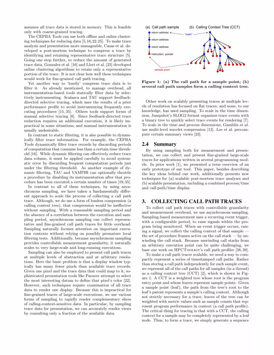
(a) Call path sample (b) Calling Context Tree (CCT)
“main”
sample point
Figure 1: (a) The call path for a sample point; (b)several call path samples form a calling context tree.
Other work on scalably presenting traces at multiple lev-els of resolution has focused on flat traces; and none, to ourknowledge, has used sampling. To scale in the time dimen-sion, Jumpshot’s SLOG2 format organizes trace events witha binary tree to quickly select trace events for rendering [7].To scale in the time and process dimensions, Gamblin et al.use multi-level wavelet compression [12]. Lee et al. precom-pute certain summary views [23].
2.4 SummaryBy using sampling both for measurement and presen-
tation, we can collect and present fine-grained large-scaletraces for applications written in several programming mod-els. In prior work [1], we presented a terse overview of anearly prototype of our tool. This paper, besides describingthe key ideas behind our work, additionally presents newtechniques for (a) scalable post-mortem trace analyses and(b) scalable presentation, including a combined process/timeand call-path/time display.
3. COLLECTING CALL PATH TRACESTo collect call path traces with controllable granularity
and measurement overhead, we use asynchronous sampling.Sampling-based measurement uses a recurring event trigger,with a configurable period, to raise signals within the pro-gram being monitored. When an event trigger occurs, rais-ing a signal, we collect the calling context of that sample —the set of procedure frames active on the call stack — by un-winding the call stack. Because unwinding call stacks froman arbitrary execution point can be quite challenging, webase our work on HPCToolkit’s call path profiler [38,39].
To make a call path tracer scalable, we need a way to com-pactly represent a series of timestamped call paths. Ratherthan storing a call path independently for each sample event,we represent all of the call paths for all samples (in a thread)as a calling context tree (CCT) [2], which is shown in Fig-ure 1. A CCT is a weighted tree whose root is the programentry point and whose leaves represent sample points. Givena sample point (leaf), the path from the tree’s root to theleaf’s parent represents a sample’s calling context. Althoughnot strictly necessary for a trace, leaves of the tree can beweighted with metric values such as sample counts that rep-resent program performance in context (a call path profile).The critical thing for tracing is that with a CCT, the callingcontext for a sample may be completely represented by a leafnode. Thus, to form a trace, we simply generate a sequence
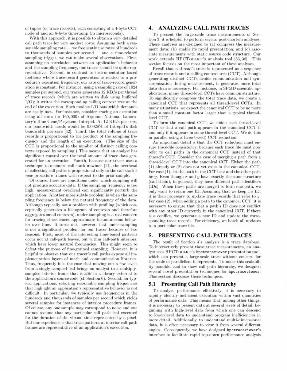
of tuples (or trace records), each consisting of a 4-byte CCTnode id and an 8-byte timestamp (in microseconds).
With this approach, it is possible to obtain a very detailedcall path trace for very modest costs. Assuming both a rea-sonable sampling rate — we frequently use rates of hundredsto thousands of samples per second — and a time-relatedsampling trigger, we can make several observations. First,assuming no correlation between an application’s behaviorand the sampling frequency, our traces should be quite rep-resentative. Second, in contrast to instrumentation-basedmethods where trace-record generation is related to a pro-cedure’s execution frequency, our rate of trace-record gener-ation is constant. For instance, using a sampling rate of 1024samples per second, our tracer generates 12 KB/s per threadof trace records (which are written to disk using bufferedI/O); it writes the corresponding calling context tree at theend of the execution. Such modest I/O bandwidth demandsare easily met. For instance, consider tracing an executionusing all cores (≈ 160, 000) of Argonne National Labora-tory’s Blue Gene/P system, Intrepid. At 12 KB/s per core,our bandwidth needs would be 0.0028% of Intrepid’s diskbandwidth per core [42]. Third, the total volume of tracerecords is proportional to the product of the sampling fre-quency and the length of an execution. (The size of theCCT is proportional to the number of distinct calling con-texts exposed by sampling.) This means that an analyst hassignificant control over the total amount of trace data gen-erated for an execution. Fourth, because our tracer uses atechnique to memoize call stack unwinds [11], the overheadof collecting call paths is proportional only to the call stack’snew procedure frames with respect to the prior sample.
Of course, there are conditions under which sampling willnot produce accurate data. If the sampling frequency is toohigh, measurement overhead can significantly perturb theapplication. Another more subtle problem is when the sam-pling frequency is below the natural frequency of the data.Although typically not a problem with profiling (which con-ceptually generates a histogram of contexts and thereforeaggregates small contexts), under-sampling is a real concernfor tracing since traces approximate instantaneous behav-ior over time. It turns out, however, that under-samplingis not a significant problem for our tracer because of tworeasons. First, most of the interesting time-based patternsoccur not at call-path leaves, but within call-path interiors,which have lower natural frequencies. This might seem todefeat the purpose of fine-grained sampling. However, it ishelpful to observe that our tracer’s call paths expose all im-plementation layers of math and communication libraries.Thus, frequently it is the case that moving out a few levelsfrom a singly-sampled leaf brings an analyst to a multiply-sampled interior frame that is still in a library external tothe application’s source code (cf. Section 6). Second, for typ-ical applications, selecting reasonable sampling frequenciesthat highlight an application’s representative behavior is notdifficult. In particular, we typically use frequencies in thehundreds and thousands of samples per second which yieldsseveral samples for instances of interior procedure frames.Of course, any one sample may correspond to noise and onecannot assume that any particular call path leaf executedfor the duration of the virtual time represented by a pixel.But our experience is that trace patterns at interior call-pathframes are representative of an application’s execution.
4. ANALYZING CALL PATH TRACESTo present the large-scale trace measurements of Sec-
tion 3, it is helpful to perform several post-mortem analyses.These analyses are designed to (a) compress the measure-ment data; (b) enable its rapid presentation; and (c) asso-ciate measurements with static source code structure. Ourwork extends HPCToolkit’s analysis tool [36, 38]. Thissection focuses on the most important of these analyses.
Recall that a thread’s trace is represented as a sequenceof trace records and a calling context tree (CCT). Althoughgenerating distinct CCTs avoids communication and syn-chronization during measurement, it generates more totaldata than is necessary. For instance, in SPMD scientific ap-plications, many thread-level CCTs have common structure.To significantly compress the total trace data, we create acanonical CCT that represents all thread-level CCTs. Inmany situations, we expect the canonical CCT to be no morethan a small constant factor larger than a typical thread-level CCT.
To form the canonical CCT, we union each thread-levelCCT so that a call path appears in the canonical CCT ifand only if it appears in some thread-level CCT. We do thisin parallel using a (tree-based) CCT reduction.
An important detail is that the CCT reduction must en-sure trace-file consistency, because each trace file must nowrefer to call paths in the canonical CCT instead of thatthread’s CCT. Consider the case of merging a path from athread-level CCT into the canonical CCT. Either the path(1) already or (2) does not yet exist in the canonical CCT.For case (1), let the path in the CCT be x and the other pathbe y. Even though x and y have exactly the same structure(call chain), in general, they have different path identifiers(IDs). When these paths are merged to form one path, weonly want to retain one ID. Assuming that we keep x’s ID,it is then necessary to update trace records that refer to y.For case (2), when adding a path to the canonical CCT, it isnecessary to ensure that that a path’s ID does not conflictwith any other ID currently in the canonical CCT. If thereis a conflict, we generate a new ID and update the corre-sponding trace records. For efficiency, we batch all updatesto a particular trace file.
5. PRESENTING CALL PATH TRACESThe result of Section 4’s analysis is a trace database.
To interactively present these trace measurements, an ana-lyst uses HPCToolkit’s hpctraceviewer presentation tool,which can present a large-scale trace without concern forthe scale of parallelism it represents. To make this scalabil-ity possible, and to show call path hierarchy, we designedseveral novel presentation techniques for hpctraceviewer.This section discusses those techniques.
5.1 Presenting Call Path HierarchyTo analyze performance effectively, it is necessary to
rapidly identify inefficient execution within vast quantitiesof performance data. This means that, among other things,it is necessary to present data at several levels of detail, be-ginning with high-level data from which one can descendto lower-level data to understand program inefficiencies inmore detail. Additionally, to understand multi-dimensionaldata, it is often necessary to view it from several differentangles. Consequently, we have designed hpctraceviewer’sinterface to facilitate rapid top-down performance analysis
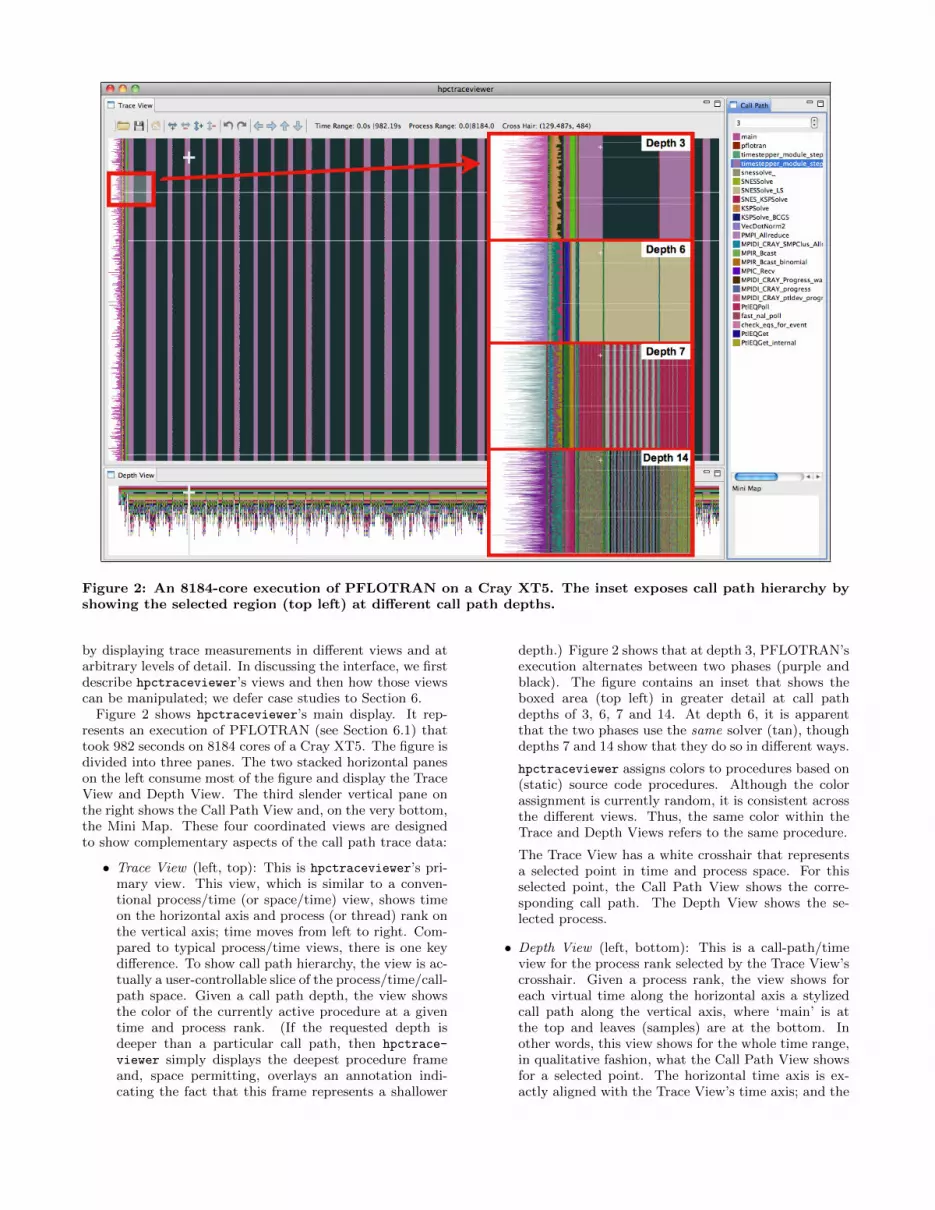
Figure 2: An 8184-core execution of PFLOTRAN on a Cray XT5. The inset exposes call path hierarchy byshowing the selected region (top left) at different call path depths.
by displaying trace measurements in different views and atarbitrary levels of detail. In discussing the interface, we firstdescribe hpctraceviewer’s views and then how those viewscan be manipulated; we defer case studies to Section 6.
Figure 2 shows hpctraceviewer’s main display. It rep-resents an execution of PFLOTRAN (see Section 6.1) thattook 982 seconds on 8184 cores of a Cray XT5. The figure isdivided into three panes. The two stacked horizontal paneson the left consume most of the figure and display the TraceView and Depth View. The third slender vertical pane onthe right shows the Call Path View and, on the very bottom,the Mini Map. These four coordinated views are designedto show complementary aspects of the call path trace data:
• Trace View (left, top): This is hpctraceviewer’s pri-mary view. This view, which is similar to a conven-tional process/time (or space/time) view, shows timeon the horizontal axis and process (or thread) rank onthe vertical axis; time moves from left to right. Com-pared to typical process/time views, there is one keydifference. To show call path hierarchy, the view is ac-tually a user-controllable slice of the process/time/call-path space. Given a call path depth, the view showsthe color of the currently active procedure at a giventime and process rank. (If the requested depth isdeeper than a particular call path, then hpctrace-
viewer simply displays the deepest procedure frameand, space permitting, overlays an annotation indi-cating the fact that this frame represents a shallower
depth.) Figure 2 shows that at depth 3, PFLOTRAN’sexecution alternates between two phases (purple andblack). The figure contains an inset that shows theboxed area (top left) in greater detail at call pathdepths of 3, 6, 7 and 14. At depth 6, it is apparentthat the two phases use the same solver (tan), thoughdepths 7 and 14 show that they do so in different ways.
hpctraceviewer assigns colors to procedures based on(static) source code procedures. Although the colorassignment is currently random, it is consistent acrossthe different views. Thus, the same color within theTrace and Depth Views refers to the same procedure.
The Trace View has a white crosshair that representsa selected point in time and process space. For thisselected point, the Call Path View shows the corre-sponding call path. The Depth View shows the se-lected process.
• Depth View (left, bottom): This is a call-path/timeview for the process rank selected by the Trace View’scrosshair. Given a process rank, the view shows foreach virtual time along the horizontal axis a stylizedcall path along the vertical axis, where ‘main’ is atthe top and leaves (samples) are at the bottom. Inother words, this view shows for the whole time range,in qualitative fashion, what the Call Path View showsfor a selected point. The horizontal time axis is ex-actly aligned with the Trace View’s time axis; and the
colors are consistent across both views. This view hasits own crosshair that corresponds to the currently se-lected time and call path depth.
• Call Path View (right, top): This view shows twothings: (1) the current call path depth that definesthe hierarchical slice shown in the Trace View; and (2)the actual call path for the point selected by the TraceView’s crosshair. (To easily coordinate the call pathdepth value with the call path, the Call Path Viewcurrently suppresses details such as loop structure andcall sites; we may use indentation or other techniquesto display this in the future.)
• Mini Map (right, bottom): The Mini Map shows, rela-tive to the process/time dimensions, the portion of theexecution shown by the Trace View. The Mini Map en-ables one to zoom and to move from one close-up toanother quickly.
To further support top-down analysis, hpctraceviewer
includes several controls for changing a view’s aspect andnavigating through various levels of data:
• The Trace View can be zoomed arbitrarily in both ofits process and time dimensions. To zoom in both di-mensions at once, one may (a) select a sub-region ofthe current view; or (b) select an arbitrary region ofthe Mini Map. To zoom in only one of the above di-mensions, one may use the appropriate control buttonsat the top of the Trace View. At any time, one may re-turn to the entire execution’s view by using the ‘Home’button.
• To expose call path hierarchy, the call-path-depth sliceshown in the Trace View can be changed by using theCall Path View’s depth text box or by selecting a pro-cedure frame within the Call Path View.
• To pan the Trace and Depth Views horizontally or ver-tically, one may (a) use buttons at the top of the TraceView pane; or (b) adjust the Mini Map’s current focus.
Even though hpctraceviewer supports panning, it is worthnoting that zooming is much more important because it per-mits viewing the execution at different levels of abstraction.In contrast, a tool that requires scrolling through vast quan-tities of data is difficult to use because, at any one time, thetool can only present a fraction of the execution.
5.2 Using Sampling for Scalable PresentationTo implement the arbitrary zooming that is required to
support top-down analysis, it is clearly not feasible either(a) to examine all trace data repeatedly and exhaustively or(b) to precompute all possible (or likely) views. One possi-ble solution for displaying data at multiple resolutions is toprecompute select summary views [23]. We prefer a methodthat dynamically and rapidly renders views at arbitrary res-olutions.
Consider a large-scale execution that has tens of thou-sands of processor ranks and that runs for thousands ofseconds, where time granularity is a microsecond. A traceof this scale dwarfs any typical computer display; today,a high-end 30-inch display we use has a width and heightof 2560× 1600 pixels. Thus, the basic problem that a trace
presentation tool faces is the following: Given a display win-dow of a certain size, how should that window be renderedin time that is proportional not to the total amount of tracedata, but to the window size? Alternatively, we can ask:given that one pixel maps to many trace records from manyprocess ranks, how should we color that pixel without con-sulting all of the associated trace records?
In this connection, it is helpful to briefly consider the pre-sentation technique of conveying the maximum possible in-formation about an application’s behavior [22]; cf. [23]. Forexample, to color one pixel, one could use either the mini-mum or maximum of the metric values associated with thetrace records mapped to the pixel. While this can be a veryeffective way of rendering performance, it limits the scala-bility of a presentation tool because it requires examiningevery trace record mapped to the pixel.
In contrast, to render the views described in Section 5.1without concern for the scale of parallelism they represent,we use various forms of sampling. For example, consider theTrace View, which displays procedures at a given call pathdepth along the process and time axes. To render this viewin a display window of height h and width w, hpctrace-
viewer does two things. First, it systematically samples theexecution’s process ranks to select h ranks and their corre-sponding trace files. (For the trivial case where the numberof process ranks is less than or equal to h, all ranks are repre-sented.) Second, hpctraceviewer uses a form of systematicsampling to select the call path frames displayed along theprocess rank’s time lines. It subdivides the time interval rep-resented by the entire execution into a series of consecutiveand equal intervals using w virtual timestamps. Then, foreach virtual timestamp, it binary searches the correspond-ing trace file — our trace file format is effectively a vectorof trace records — to locate the record with the closest ac-tual timestamp; this record’s call path is used to define thepixel’s color.
We can make several observations about this scheme. Be-cause we consult at most h trace files and perform at mostw binary searches in each trace file, the time it takes to ren-der the Trace View is O(hw log t), where t is the number oftrace records in the largest trace file. In practice, the log tfactor is often negligible because we use linear extrapola-tion to predict the locations of the w trace records. Next,as with the Trace View, the Depth View can also be ren-dered in time O(hw log t) by considering at most h framesof each call path. For some zooms and scrolling it is possibleto reuse previously computed information to further reducerendering costs. Finally, by generating virtual timestampsand using binary search, we effectively overlay a binary treeon the trace data, which is the basic idea behind Jumpshot’sSLOG2 trace format [7].
One problem with sampling-based methods is that whilethey tend to show representative behavior, they might missinteresting extreme behavior. While this will always be aproblem with statistical methods, two things attenuate theseconcerns. First, we (scalably) precompute special constant-sized values (instead of views) for hpctraceviewer. For ex-ample, we compute, for all trace files, the minimum begin-ning timestamp and the maximum ending timestamp, whichtakes work proportional to the number of processor ranks.Though a minor contribution, these timestamps enable hpc-traceviewer’s Trace View to expose, e.g., extreme variationin an application’s launch or teardown. Second, and more
to the point, assuming an appropriately sized and uncor-related sample, we expect sampling-based methods to ex-pose anomalies that generally affect an execution. In otherwords, although using sampling-based methods for render-ing a high-level view can easily miss a specific anomaly, thosesame methods will expose the anomaly’s general effects. Ifthe anomaly does not interfere with the application’s exe-cution, then a high-level view will show no effects. But ifprocess synchronization transfers the anomaly’s effects toother process ranks, we expect sampling-based methods toexpose that fact. It is worth noting that Figure 2 actuallyexposes an interesting anomaly. The thin horizontal whitelines in the Trace View represent a few processes for whichsampling simply stopped, most likely (we suspect) becauseof a kernel bug.2 One possible avenue of future work is for ananalyst to identify a region and request a more exhaustiveroot-cause analysis.
We are currently working on a Summary View that showsfor each virtual timestamp a stacked histogram that quali-tatively represents the number of process ranks executing agiven procedure at a given call path depth. This view wouldbe similar to Vampir’s ‘Summary Timeline’ [19]. However,in contrast to Vampir, which, to our knowledge, computesits view based on examining the activity of each thread ateach time interval, we will use a sampling-based method toscalably render the view. To render this view for a windowof height h and width w, we will first generate a series of wvirtual timestamps as with the Trace View. Then, to createa stacked histogram for a given virtual timestamp, we willtake a random sample of the process ranks and from theredetermine the set of currently executing procedures. Thetime complexity of rendering this view is the same as for theTrace View.
Unlike many other tools, hpctraceviewer does not renderinter-process communication arcs. We are uncertain how todo this effectively and scalably. Instead, we are exploringways of using a special color, say red, to indicate, at all levelsof a call path, when a sample corresponds to communication.
6. CASE STUDIESTo demonstrate the ability of our tracing techniques to
yield insight into the performance of parallel executions,we apply them to study the performance of the PFLO-TRAN ground water flow simulation application [26, 29];the FLASH [10] astrophysical thermonuclear flash code; andtwo HPC Challenge benchmark codes [18] written in Coar-ray Fortran 2.0, one implementing a parallel one-dimensionalFast Fourier Transform (FFT), and the second implementingHigh Performance Linpack, (HPL) which solves a dense lin-ear system on distributed memory computers. We describeour experiences with each of these applications in turn.
6.1 PFLOTRANPFLOTRAN models multi-phase, multi-component sub-
surface flow and reactive transport on massively parallelcomputers [26, 29]. It uses the PETSc [4] library’s Newton-Krylov solver framework.
We collected call path traces of PFLOTRAN running on8184 cores of a Cray XT5 system known as JaguarPF, which
2This process could not have stopped because the execu-tion’s many successful collective-communication operationswould not have completed.
is installed at Oak Ridge National Laboratory. The input forthe PFLOTRAN run was a steady-state groundwater flowproblem. To collect traces, we configured HPCToolkit’shpcrun to sample wallclock time at a frequency of 200 sam-ples/second. Tracing dilated the application’s execution by5% and the total job (including the time for hpcrun to flushmeasurements to disk) by 10%. hpcrun generated 13 GB ofdata (1.6 MB/process); a parallel version of HPCToolkit’shpcprof analyzed the measurements in 13.5 minutes using48 cores and generated a 7.5 GB trace database.
Figure 2 shows hpctraceviewer displaying a high leveloverview of a complete call path trace of a 16 minute execu-tion of PFLOTRAN on 8184 cores. Recall from Section 5.1that (a) the Trace View (top) shows a process/time view;(b) the Depth View shows a time-line view of the call pathfor the selected process; and (c) the Call Path View (right)shows a call path for the selected time and process. A pro-cess’s activity over time unfolds from left to right.
Unlike other trace visualizers, hpctraceviewer’s visual-izations are hierarchical. Since each sample in each process’stimeline represents a call path, we can view the process time-lines at different call path depths to show more or less de-tailed views of the execution. The figure shows the executionat a call path depth of 3. Each distinct color on the timelinesrepresents a different procedure executing at this depth. Thefigure clearly shows the alternation between PFLOTRAN’sflow (purple) and transport (black) phases. The beginningof the execution shows different behavior as the applicationreads its input using the HDF5 library. The figure containsan inset that shows the boxed area (top left) in greater detailat call path depths of 3, 6, 7 and 14. At depth 6, it is appar-ent that the flow and transport phases use the same solver(tan), though depths 7 and 14 show that they do so in differ-ent ways. The point selected by the crosshair shows the flowphase performing an MPI_Allreduce on behalf of a vectordot product (VecDotNorm2) deep within the PETSc library.The call path also descends into Cray’s MPI implementa-tion. Given that the routine MPIDI_CRAY_Progress_wait
(eighth from the bottom) is associated with exposed waiting,we can infer that the flow phase is currently busy-waiting forcollective communication to complete.
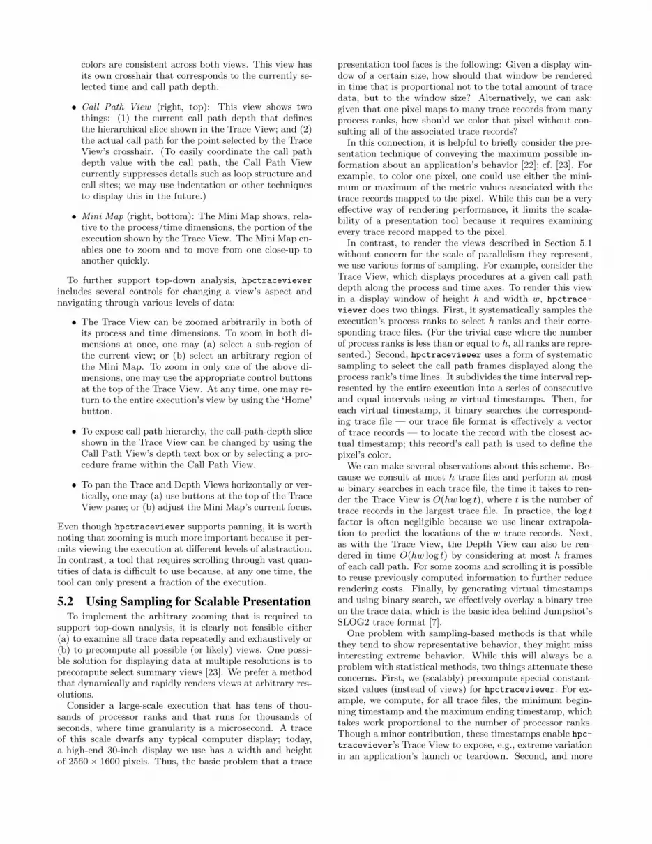
6.2 FLASHNext we consider FLASH [10], a code for modeling as-
trophysical thermonuclear flashes. Figure 3 shows hpc-
traceviewer displaying an 8184-core JaguarPF-execution ofFLASH. We used an input for simulating a white dwarf det-onation. It is immediately apparent that the first 60% ofexecution is quite different than the regular patterns thatappear thereafter. The Trace View’s crosshair marks theapproximate transition point. At this point, the Call PathView makes clear that the execution is still in its initial-ization phase (cf. driver_initflash at depth 2). Note thelarge light purple region on the left that consumes aboutone-third of the execution. A small amount of additionalinspection reveals that this corresponds to a routine whichsimply calls MPI_Init. Note also that there are a few whitelines that span the length of this light purple segment. Theselines correspond to straggler MPI ranks which took about190 seconds to launch — no samples can be collected untila process starts — and arrive at MPI_Init, which is act-ing like a collective operation. In other words, recalling thediscussion in Section 5.2, a few anomalous processors had
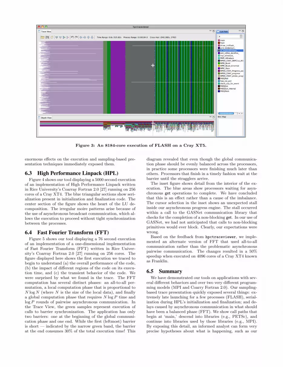
Figure 3: An 8184-core execution of FLASH on a Cray XT5.
enormous effects on the execution and sampling-based pre-sentation techniques immediately exposed them.
6.3 High Performance Linpack (HPL)Figure 4 shows our tool displaying a 5000 second execution
of an implementation of High Performance Linpack writtenin Rice University’s Coarray Fortran 2.0 [27] running on 256cores of a Cray XT4. The blue triangular sections show seri-alization present in initialization and finalization code. Thecenter section of the figure shows the heart of the LU de-composition. The irregular moire patterns arise because ofthe use of asynchronous broadcast communication, which al-lows the execution to proceed without tight synchronizationbetween the processes.
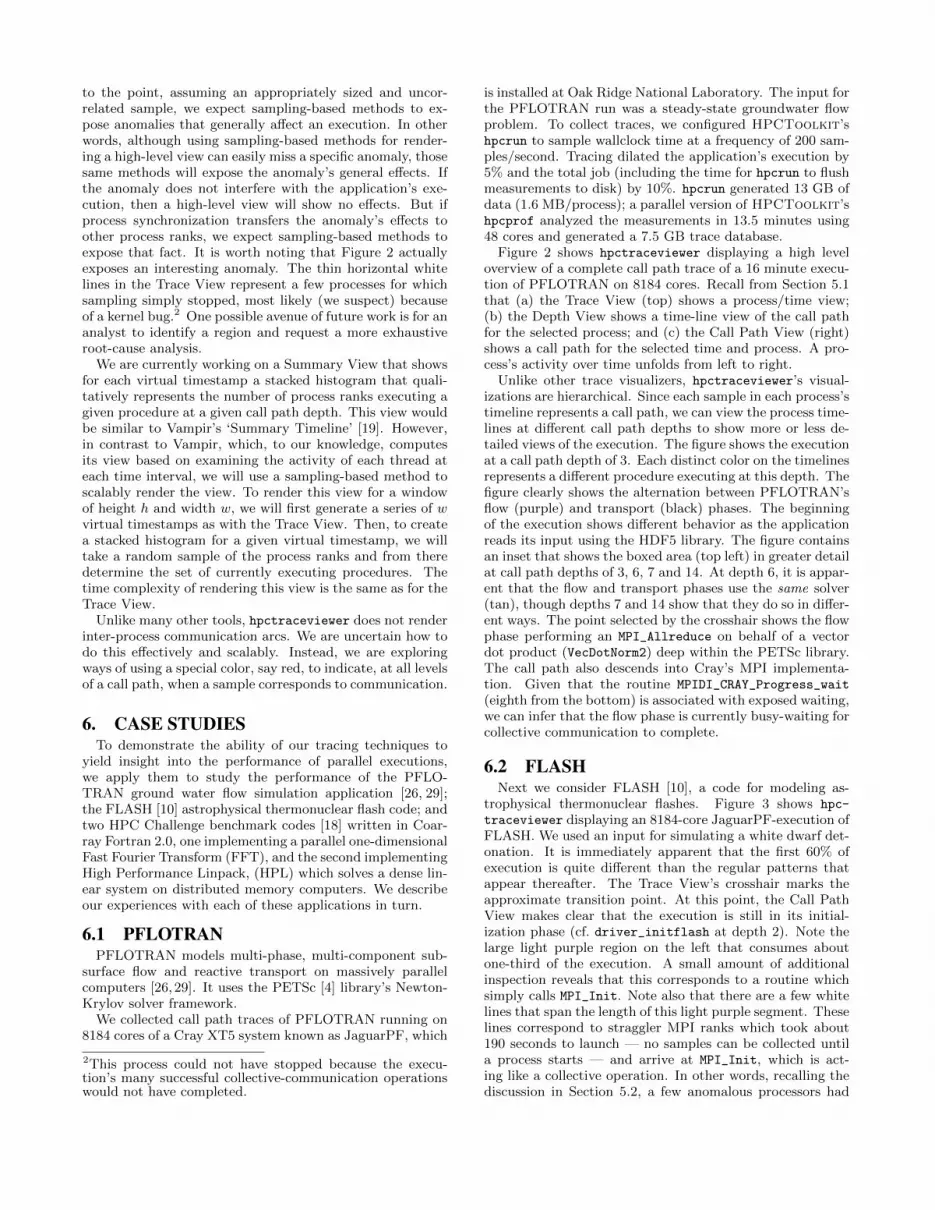
6.4 Fast Fourier Transform (FFT)Figure 5 shows our tool displaying a 76 second execution
of an implementation of a one-dimensional implementationof Fast Fourier Transform (FFT) written in Rice Univer-sity’s Coarray Fortran 2.0 [27] running on 256 cores. Thefigure displayed here shows the first execution we traced tobegin to understand (a) the overall performance of the code,(b) the impact of different regions of the code on its execu-tion time, and (c) the transient behavior of the code. Wewere surprised by what we found in the trace. The FFTcomputation has several distinct phases: an all-to-all per-mutation, a local computation phase that is proportional toN logN (where N is the size of the local data), and finallya global computation phase that requires N logP time andlogP rounds of pairwise asynchronous communication. Inthe Trace View, the green samples represent execution ofcalls to barrier synchronization. The application has onlytwo barriers: one at the beginning of the global communi-cation phase and one end. While the first (leftmost) barrieris short — indicated by the narrow green band, the barrierat the end consumes 30% of the total execution time! This
diagram revealed that even though the global communica-tion phase should be evenly balanced across the processors,in practice some processors were finishing much later thanothers. Processors that finish in a timely fashion wait at thebarrier until the stragglers arrive.
The inset figure shows detail from the interior of the ex-ecution. The blue areas show processors waiting for asyn-chronous get operations to complete. We have concludedthat this is an effect rather than a cause of the imbalance.The cursor selection in the inset shows an unexpected stallinside our asynchronous progress engine. The stall occurredwithin a call to the GASNet communication library thatchecks for the completion of a non-blocking get. In our use ofGASNet, we had not anticipated that calls to non-blockingprimitives would ever block. Clearly, our expectations werewrong.
Based on the feedback from hpctraceviewer, we imple-mented an alternate version of FFT that used all-to-allcommunication rather than the problematic asynchronouspairwise communication. The changes resulted in a 50%speedup when executed on 4096 cores of a Cray XT4 knownas Franklin.
6.5 SummaryWe have demonstrated our tools on applications with sev-
eral different behaviors and over two very different program-ming models (MPI and Coarry Fortran 2.0). Our sampling-based trace presentation quickly exposed several things: ex-tremely late launching for a few processes (FLASH), serial-ization during HPL’s initialization and finalization; and de-lays caused by asynchronous communication in what shouldhave been a balanced phase (FFT). We show call paths thatbegin at ‘main,’ descend into libraries (e.g., PETSc), andcontinue into libraries used by those libraries (e.g., MPI).By exposing this detail, an informed analyst can form veryprecise hypotheses about what is happening, such as our
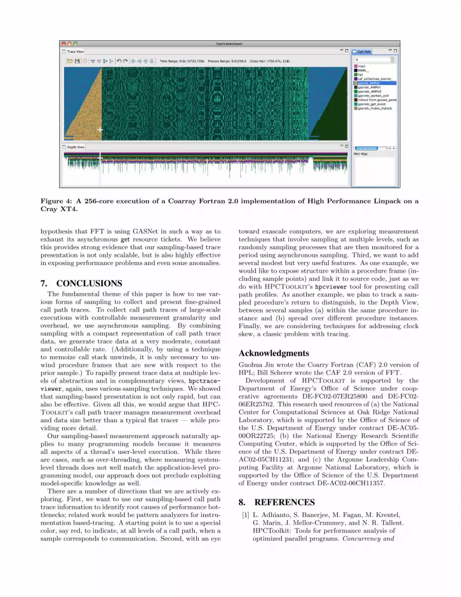
Figure 4: A 256-core execution of a Coarray Fortran 2.0 implementation of High Performance Linpack on aCray XT4.
hypothesis that FFT is using GASNet in such a way as toexhaust its asynchronous get resource tickets. We believethis provides strong evidence that our sampling-based tracepresentation is not only scalable, but is also highly effectivein exposing performance problems and even some anomalies.
7. CONCLUSIONSThe fundamental theme of this paper is how to use var-
ious forms of sampling to collect and present fine-grainedcall path traces. To collect call path traces of large-scaleexecutions with controllable measurement granularity andoverhead, we use asynchronous sampling. By combiningsampling with a compact representation of call path tracedata, we generate trace data at a very moderate, constantand controllable rate. (Additionally, by using a techniqueto memoize call stack unwinds, it is only necessary to un-wind procedure frames that are new with respect to theprior sample.) To rapidly present trace data at multiple lev-els of abstraction and in complementary views, hpctrace-viewer, again, uses various sampling techniques. We showedthat sampling-based presentation is not only rapid, but canalso be effective. Given all this, we would argue that HPC-Toolkit’s call path tracer manages measurement overheadand data size better than a typical flat tracer — while pro-viding more detail.
Our sampling-based measurement approach naturally ap-plies to many programming models because it measuresall aspects of a thread’s user-level execution. While thereare cases, such as over-threading, where measuring system-level threads does not well match the application-level pro-gramming model, our approach does not preclude exploitingmodel-specific knowledge as well.
There are a number of directions that we are actively ex-ploring. First, we want to use our sampling-based call pathtrace information to identify root causes of performance bot-tlenecks; related work would be pattern analyzers for instru-mentation based-tracing. A starting point is to use a specialcolor, say red, to indicate, at all levels of a call path, when asample corresponds to communication. Second, with an eye
toward exascale computers, we are exploring measurementtechniques that involve sampling at multiple levels, such asrandomly sampling processes that are then monitored for aperiod using asynchronous sampling. Third, we want to addseveral modest but very useful features. As one example, wewould like to expose structure within a procedure frame (in-cluding sample points) and link it to source code, just as wedo with HPCToolkit’s hpcviewer tool for presenting callpath profiles. As another example, we plan to track a sam-pled procedure’s return to distinguish, in the Depth View,between several samples (a) within the same procedure in-stance and (b) spread over different procedure instances.Finally, we are considering techniques for addressing clockskew, a classic problem with tracing.
AcknowledgmentsGuohua Jin wrote the Coarry Fortran (CAF) 2.0 version ofHPL; Bill Scherer wrote the CAF 2.0 version of FFT.
Development of HPCToolkit is supported by theDepartment of Energy’s Office of Science under coop-erative agreements DE-FC02-07ER25800 and DE-FC02-06ER25762. This research used resources of (a) the NationalCenter for Computational Sciences at Oak Ridge NationalLaboratory, which is supported by the Office of Science ofthe U.S. Department of Energy under contract DE-AC05-00OR22725; (b) the National Energy Research ScientificComputing Center, which is supported by the Office of Sci-ence of the U.S. Department of Energy under contract DE-AC02-05CH11231; and (c) the Argonne Leadership Com-puting Facility at Argonne National Laboratory, which issupported by the Office of Science of the U.S. Departmentof Energy under contract DE-AC02-06CH11357.
8. REFERENCES[1] L. Adhianto, S. Banerjee, M. Fagan, M. Krentel,
G. Marin, J. Mellor-Crummey, and N. R. Tallent.HPCToolkit: Tools for performance analysis ofoptimized parallel programs. Concurrency and
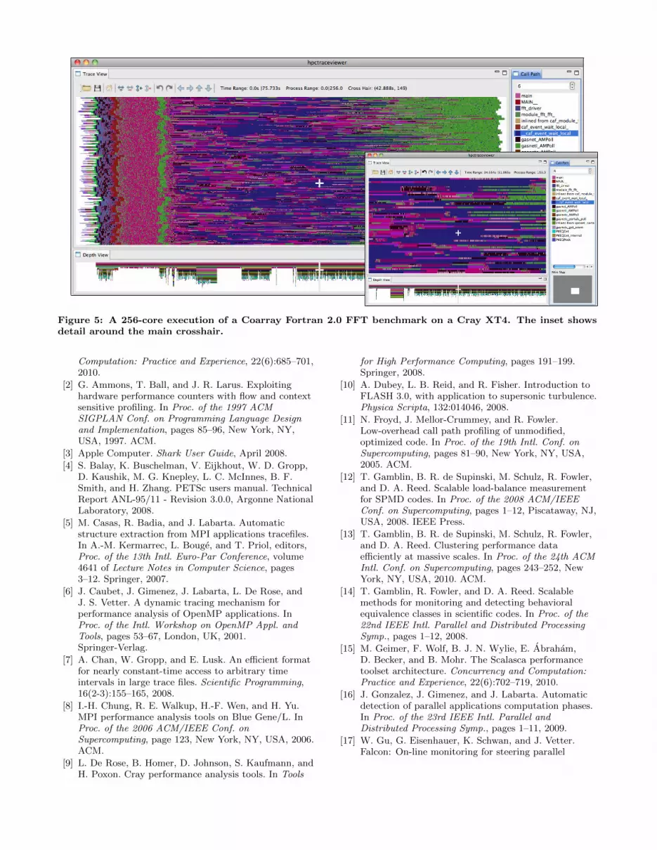
Figure 5: A 256-core execution of a Coarray Fortran 2.0 FFT benchmark on a Cray XT4. The inset showsdetail around the main crosshair.
Computation: Practice and Experience, 22(6):685–701,2010.
[2] G. Ammons, T. Ball, and J. R. Larus. Exploitinghardware performance counters with flow and contextsensitive profiling. In Proc. of the 1997 ACMSIGPLAN Conf. on Programming Language Designand Implementation, pages 85–96, New York, NY,USA, 1997. ACM.
[3] Apple Computer. Shark User Guide, April 2008.
[4] S. Balay, K. Buschelman, V. Eijkhout, W. D. Gropp,D. Kaushik, M. G. Knepley, L. C. McInnes, B. F.Smith, and H. Zhang. PETSc users manual. TechnicalReport ANL-95/11 - Revision 3.0.0, Argonne NationalLaboratory, 2008.
[5] M. Casas, R. Badia, and J. Labarta. Automaticstructure extraction from MPI applications tracefiles.In A.-M. Kermarrec, L. Bouge, and T. Priol, editors,Proc. of the 13th Intl. Euro-Par Conference, volume4641 of Lecture Notes in Computer Science, pages3–12. Springer, 2007.
[6] J. Caubet, J. Gimenez, J. Labarta, L. De Rose, andJ. S. Vetter. A dynamic tracing mechanism forperformance analysis of OpenMP applications. InProc. of the Intl. Workshop on OpenMP Appl. andTools, pages 53–67, London, UK, 2001.Springer-Verlag.
[7] A. Chan, W. Gropp, and E. Lusk. An efficient formatfor nearly constant-time access to arbitrary timeintervals in large trace files. Scientific Programming,16(2-3):155–165, 2008.
[8] I.-H. Chung, R. E. Walkup, H.-F. Wen, and H. Yu.MPI performance analysis tools on Blue Gene/L. InProc. of the 2006 ACM/IEEE Conf. onSupercomputing, page 123, New York, NY, USA, 2006.ACM.
[9] L. De Rose, B. Homer, D. Johnson, S. Kaufmann, andH. Poxon. Cray performance analysis tools. In Tools
for High Performance Computing, pages 191–199.Springer, 2008.
[10] A. Dubey, L. B. Reid, and R. Fisher. Introduction toFLASH 3.0, with application to supersonic turbulence.Physica Scripta, 132:014046, 2008.
[11] N. Froyd, J. Mellor-Crummey, and R. Fowler.Low-overhead call path profiling of unmodified,optimized code. In Proc. of the 19th Intl. Conf. onSupercomputing, pages 81–90, New York, NY, USA,2005. ACM.
[12] T. Gamblin, B. R. de Supinski, M. Schulz, R. Fowler,and D. A. Reed. Scalable load-balance measurementfor SPMD codes. In Proc. of the 2008 ACM/IEEEConf. on Supercomputing, pages 1–12, Piscataway, NJ,USA, 2008. IEEE Press.
[13] T. Gamblin, B. R. de Supinski, M. Schulz, R. Fowler,and D. A. Reed. Clustering performance dataefficiently at massive scales. In Proc. of the 24th ACMIntl. Conf. on Supercomputing, pages 243–252, NewYork, NY, USA, 2010. ACM.
[14] T. Gamblin, R. Fowler, and D. A. Reed. Scalablemethods for monitoring and detecting behavioralequivalence classes in scientific codes. In Proc. of the22nd IEEE Intl. Parallel and Distributed ProcessingSymp., pages 1–12, 2008.
[15] M. Geimer, F. Wolf, B. J. N. Wylie, E. Abraham,D. Becker, and B. Mohr. The Scalasca performancetoolset architecture. Concurrency and Computation:Practice and Experience, 22(6):702–719, 2010.
[16] J. Gonzalez, J. Gimenez, and J. Labarta. Automaticdetection of parallel applications computation phases.In Proc. of the 23rd IEEE Intl. Parallel andDistributed Processing Symp., pages 1–11, 2009.
[17] W. Gu, G. Eisenhauer, K. Schwan, and J. Vetter.Falcon: On-line monitoring for steering parallel
programs. Concurrency: Practice and Experience,10(9):699–736, 1998.
[18] Innovative Computing Laboratory, University ofTennessee. HPC Challenge benchmarks.http://icl.cs.utk.edu/hpcc.
[19] A. Knupfer, H. Brunst, J. Doleschal, M. Jurenz,M. Lieber, H. Mickler, M. S. Muller, and W. E. Nagel.The Vampir performance analysis tool-set. InM. Resch, R. Keller, V. Himmler, B. Krammer, andA. Schulz, editors, Tools for High PerformanceComputing, pages 139–155. Springer, 2008.
[20] A. Knupfer and W. Nagel. Construction andcompression of complete call graphs for post-mortemprogram trace analysis. In Proc. of the 2005 Intl.Conf. on Parallel Processing, pages 165–172, 2005.
[21] J. Labarta. Obtaining extremely detailed informationat scale. 2009 Workshop on Performance Tools forPetascale Computing (Center for Scalable ApplicationDevelopment Software), July 2009.
[22] J. Labarta, J. Gimenez, E. Martınez, P. Gonzalez,H. Servat, G. Llort, and X. Aguilar. Scalability ofvisualization and tracing tools. In G. Joubert,W. Nagel, F. Peters, O. Plata, P. Tirado, andE. Zapata, editors, Parallel Computing: Current &Future Issues of High-End Computing: Proc. of theIntl. Conf. ParCo 2005, volume 33 of NIC Series,pages 869–876, Julich, September 2006. John vonNeumann Institute for Computing.
[23] C. W. Lee and L. V. Kale. Scalable techniques forperformance analysis. Technical Report 07-06, Dept.of Computer Science, University of Illinois,Urbana-Champaign, May 2007.
[24] C. W. Lee, C. Mendes, and L. V. Kale. Towardsscalable performance analysis and visualizationthrough data reduction. In Proc. of the 22nd IEEEIntl. Parallel and Distributed Processing Symp., pages1–8, 2008.
[25] G. Llort, J. Gonzalez, H. Servat, J. Gimenez, andJ. Labarta. On-line detection of large-scale parallelapplication’s structure. In Proc. of the 24th IEEE Intl.Parallel and Distributed Processing Symp., pages 1–10,2010.
[26] Los Alamos National Laboratory. PFLOTRANproject. https://software.lanl.gov/pflotran, 2010.
[27] J. Mellor-Crummey, L. Adhianto, G. Jin, and W. N.Scherer III. A new vision for Coarray Fortran. In Proc.of the Third Conf. on Partitioned Global AddressSpace Programming Models, 2009.
[28] Message Passing Interface Forum. MPI: A MessagePassing Interface Standard, June 1999.http://www.mpi-forum.org/docs/mpi-11.ps.
[29] R. T. Mills, G. E. Hammond, P. C. Lichtner,V. Sripathi, G. K. Mahinthakumar, and B. F. Smith.Modeling subsurface reactive flows usingleadership-class computing. Journal of Physics:Conference Series, 180(1):012062, 2009.
[30] M. Noeth, P. Ratn, F. Mueller, M. Schulz, and B. R.de Supinski. ScalaTrace: Scalable compression andreplay of communication traces for high-performancecomputing. J. Parallel Distrib. Comput.,69(8):696–710, 2009.
[31] Oracle. Oracle Solaris Studio 12.2: PerformanceAnalyzer. http://download.oracle.com/docs/cd/E18659_01/pdf/821-1379.pdf, September 2010.
[32] Rice University. HPCToolkit performance tools.http://hpctoolkit.org.
[33] M. Schulz, J. Galarowicz, D. Maghrak, W. Hachfeld,D. Montoya, and S. Cranford. Open|SpeedShop: Anopen source infrastructure for parallel performanceanalysis. Sci. Program., 16(2-3):105–121, 2008.
[34] H. Servat, G. Llort, J. Gimenez, and J. Labarta.Detailed performance analysis using coarse grainsampling. In H.-X. Lin, M. Alexander, M. Forsell,A. Knupfer, R. Prodan, L. Sousa, and A. Streit,editors, Euro-Par 2009 Workshops, volume 6043 ofLecture Notes in Computer Science, pages 185–198.Springer-Verlag, 2010.
[35] S. S. Shende and A. D. Malony. The TAU parallelperformance system. Int. J. High Perform. Comput.Appl., 20(2):287–311, 2006.
[36] N. R. Tallent, L. Adhianto, and J. M.Mellor-Crummey. Scalable identification of loadimbalance in parallel executions using call pathprofiles. In Proc. of the 2010 ACM/IEEE Conf. onSupercomputing, 2010.
[37] N. R. Tallent and J. Mellor-Crummey. Effectiveperformance measurement and analysis ofmultithreaded applications. In Proc. of the 14th ACMSIGPLAN Symp. on Principles and Practice ofParallel Programming, pages 229–240, New York, NY,USA, 2009. ACM.
[38] N. R. Tallent, J. Mellor-Crummey, and M. W. Fagan.Binary analysis for measurement and attribution ofprogram performance. In Proc. of the 2009 ACMSIGPLAN Conf. on Programming Language Designand Implementation, pages 441–452, New York, NY,USA, 2009. ACM.
[39] N. R. Tallent, J. M. Mellor-Crummey, L. Adhianto,M. W. Fagan, and M. Krentel. Diagnosingperformance bottlenecks in emerging petascaleapplications. In Proc. of the 2009 ACM/IEEE Conf.on Supercomputing, pages 1–11, New York, NY, USA,2009. ACM.
[40] N. R. Tallent, J. M. Mellor-Crummey, andA. Porterfield. Analyzing lock contention inmultithreaded applications. In Proc. of the 15th ACMSIGPLAN Symp. on Principles and Practice ofParallel Programming, pages 269–280, New York, NY,USA, 2010. ACM.
[41] TU Dresden Center for Information Services and HighPerformance Computing (ZIH). VampirTrace 5.10.1user manual. http://www.tu-dresden.de/zih/vampirtrace, March 2011.
[42] V. Vishwanath, M. Hereld, K. Iskra, D. Kimpe,V. Morozov, M. E. Paper, R. Ross, and K. Yoshii.Accelerating I/O forwarding in IBM Blue Gene/Psystems. Technical Report ANL/MCS-P1745-0410,Argonne National Laboratory, April 2010.
[43] P. H. Worley. MPICL: A port of the PICL tracinglogic to MPI. http://www.epm.ornl.gov/picl.
[44] O. Zaki, E. Lusk, W. Gropp, and D. Swider. Towardscalable performance visualization with Jumpshot.High Performance Computing Applications,13(2):277–288, Fall 1999.