ray tracing gems - oapen
TRANSCRIPT
RAY TRACING GEMSHIGH-QUALITY AND REAL-TIME RENDERING WITH DXR AND OTHER APIS
EDITED BYERIC HAINESTOMAS AKENINE-MÖLLERSECTION EDITORSALEXANDER KELLERMORGAN MCGUIREJACOB MUNKBERGMATT PHARR
PETER SHIRLEYINGO WALDCHRIS WYMAN
Ray Tracing GemsHigh-Quality and Real-Time Rendering
with DXR and Other APIs
Edited by Eric Haines and Tomas Akenine-Möller
Section Editors Alexander KellerMorgan McGuireJacob MunkbergMatt PharrPeter ShirleyIngo WaldChris Wyman
Ray Tracing Gems: High-Quality and Real-Time Rendering with DXR and Other APIs
ISBN-13 (pbk): 978-1-4842-4426-5 ISBN-13 (electronic): 978-1-4842-4427-2https://doi.org/10.1007/978-1-4842-4427-2
Library of Congress Control Number: 2019934207
Copyright © 2019 by NVIDIA
Trademarked names, logos, and images may appear in this book. Rather than use a trademark symbol with every occurrence of a trademarked name, logo, or image we use the names, logos, and images only in an editorial fashion and to the benefit of the trademark owner, with no intention of infringement of the trademark. The use in this publication of trade names, trademarks, service marks, and similar terms, even if they are not identified as such, is not to be taken as an expression of opinion as to whether or not they are subject to proprietary rights.
While the advice and information in this book are believed to be true and accurate at the date of publication, neither the authors nor the editors nor the publisher can accept any legal responsibility for any errors or omissions that may be made. The publisher makes no warranty, express or implied, with respect to the material contained herein.
Open Access This book is licensed under the terms of the Creative Commons Attribution-NonCommercial-NoDerivatives 4.0 International License (http://creativecommons.org/licenses/by-nc-nd/4.0/), which permits any noncommercial use, sharing, distribution and
reproduction in any medium or format, as long as you give appropriate credit to the original author(s) and the source, provide a link to the Creative Commons license and indicate if you modified the licensed material. You do not have permission under this license to share adapted material derived from this book or parts of it.
The images or other third party material in this book are included in the book's Creative Commons license, unless indicated otherwise in a credit line to the material. If material is not included in the book's Creative Commons license and your intended use is not permitted by statutory regulation or exceeds the permitted use, you will need to obtain permission directly from the copyright holder.
Managing Director, Apress Media LLC: Welmoed SpahrAcquisitions Editor: Natalie PaoDevelopment Editor: James MarkhamCoordinating Editor: Jessica Vakili
Cover image designed by NVIDIA
Distributed to the book trade worldwide by Springer Science+Business Media New York, 233 Spring Street, 6th Floor, New York, NY 10013. Phone 1-800-SPRINGER, fax (201) 348-4505, e-mail [email protected], or visit www.springeronline.com. Apress Media, LLC is a California LLC and the sole member (owner) is Springer Science + Business Media Finance Inc (SSBM Finance Inc). SSBM Finance Inc is a Delaware corporation.
For information on translations, please e-mail [email protected], or visit www.apress.com/rights-permissions.
Apress titles may be purchased in bulk for academic, corporate, or promotional use. eBook versions and licenses are also available for most titles. For more information, reference our Print and eBook Bulk Sales web page at www.apress.com/bulk-sales.
Any source code or other supplementary material referenced by the author in this book is available to readers on GitHub via the book's product page, located at www.apress.com/9781484244265. For more detailed information, please visit www.apress.com/source-code.
Printed on acid-free paper
Edited by Eric HainesTomas Akenine-MöllerSection Editors: Alexander KellerMorgan McGuire
Jacob MunkbergMatt PharrPeter ShirleyIngo WaldChris Wyman
iii
Preface xiii
Foreword xv
Contributors xxi
Notation xliii
Table of Contents
PART I: Ray Tracing Basics 5
Chapter 1: Ray Tracing Terminology 7
1.1 Historical Notes ......................................................................................7
1.2 Definitions ...............................................................................................8
Chapter 2: What is a Ray? 15
2.1 Mathematical Description of a Ray .......................................................15
2.2 Ray Intervals..........................................................................................17
2.3 Rays in DXR ...........................................................................................18
2.4 Conclusion .............................................................................................19
Chapter 3: Introduction to DirectX Raytracing 21
3.1 Introduction ...........................................................................................21
3.2 Overview ................................................................................................21
3.3 Getting Started ......................................................................................22
3.4 The DirectX Raytracing Pipeline ...........................................................23
3.5 New HLSL Support for DirectX Raytracing ...........................................25
3.6 A Simple HLSL Ray Tracing Example ...................................................28
3.7 Overview of Host Initialization for DirectX Raytracing ..........................30
3.8 Basic DXR Initialization and Setup ........................................................31
iv
3.9 Ray Tracing Pipeline State Objects .....................................................37
3.10 Shader Tables ......................................................................................41
3.11 Dispatching Rays .................................................................................43
3.12 Digging Deeper and Additional Resources .........................................44
3.13 Conclusion ...........................................................................................45
Chapter 4: A Planetarium Dome Master Camera 49
4.1 Introduction ...........................................................................................49
4.2 Methods .................................................................................................50
4.3 Planetarium Dome Master Projection Sample Code ...........................58
Chapter 5: Computing Minima and Maxima of Subarrays 61
5.1 Motivation ..............................................................................................61
5.2 Naive Full Table Lookup ........................................................................62
5.3 The Sparse Table Method ......................................................................62
5.4 The (Recursive) Range Tree Method .....................................................64
5.5 Iterative Range Tree Queries ................................................................66
5.6 Results ..................................................................................................69
5.7 Summary ...............................................................................................69
PART II: Intersections and Efficiency 75
Chapter 6: A Fast and Robust Method for Avoiding Self- Intersection 77
6.1 Introduction ...........................................................................................77
6.2 Method ...................................................................................................78
6.3 Conclusion .............................................................................................84
Chapter 7: Precision Improvements for Ray/Sphere Intersection 87
7.1 Basic Ray/Sphere Intersection .............................................................87
7.2 Floating-Point Precision Considerations ..............................................89
7.3 Related Resources ................................................................................93
TABLE OF CONTENTS
v
Chapter 8: Cool Patches: A Geometric Approach to Ray/Bilinear Patch Intersections 95
8.1 Introduction and Prior Art .....................................................................95
8.2 GARP Details .......................................................................................100
8.3 Discussion of Results ..........................................................................102
8.4 Code.....................................................................................................105
Chapter 9: Multi-Hit Ray Tracing in DXR 111
9.1 Introduction .........................................................................................111
9.2 Implementation ...................................................................................113
9.3 Results ................................................................................................119
9.4 Conclusions .........................................................................................124
Chapter 10: A Simple Load-Balancing Scheme with High Scaling Efficiency 127
10.1 Introduction .......................................................................................127
10.2 Requirements ....................................................................................128
10.3 Load Balancing..................................................................................128
10.4 Results ..............................................................................................132
PART III: Reflections, Refractions, and Shadows 137
Chapter 11: Automatic Handling of Materials in Nested Volumes 139
11.1 Modeling Volumes .............................................................................139
11.2 Algorithm ..........................................................................................142
11.3 Limitations ........................................................................................146
Chapter 12: A Microfacet-Based Shadowing Function to Solve the Bump Terminator Problem 149
12.1 Introduction .......................................................................................149
12.2 Previous Work ...................................................................................150
12.3 Method ...............................................................................................151
12.4 Results ..............................................................................................157
TABLE OF CONTENTS
vi
Chapter 13: Ray Traced Shadows: Maintaining Real-Time Frame Rates 159
13.1 Introduction .......................................................................................159
13.2 Related Work .....................................................................................161
13.3 Ray Traced Shadows .........................................................................162
13.4 Adaptive Sampling ............................................................................164
13.5 Implementation .................................................................................171
13.6 Results ..............................................................................................175
13.7 Conclusion and Future Work ............................................................179
Chapter 14: Ray-Guided Volumetric Water Caustics in Single Scattering Media with DXR 183
14.1 Introduction .......................................................................................183
14.2 Volumetric Lighting and Refracted Light ..........................................186
14.3 Algorithm ..........................................................................................189
14.4 Implementation Details.....................................................................197
14.5 Results ..............................................................................................198
14.6 Future Work .......................................................................................200
14.7 Demo .................................................................................................200
PART IV: Sampling 205
Chapter 15: On the Importance of Sampling 207
15.1 Introduction .......................................................................................207
15.2 Example: Ambient Occlusion ............................................................208
15.3 Understanding Variance ....................................................................213
15.4 Direct Illumination ............................................................................216
15.5 Conclusion .........................................................................................221
Chapter 16: Sampling Transformations Zoo 223
16.1 The Mechanics of Sampling ..............................................................223
16.2 Introduction to Distributions .............................................................224
TABLE OF CONTENTS
vii
16.3 One-Dimensional Distributions ........................................................226
16.4 Two-Dimensional Distributions ........................................................230
16.5 Uniformly Sampling Surfaces ...........................................................234
16.6 Sampling Directions ..........................................................................239
16.7 Volume Scattering .............................................................................243
16.8 Adding to the Zoo Collection .............................................................244
Chapter 17: Ignoring the Inconvenient When Tracing Rays 247
17.1 Introduction .......................................................................................247
17.2 Motivation ..........................................................................................247
17.3 Clamping ...........................................................................................250
17.4 Path Regularization...........................................................................251
17.5 Conclusion .........................................................................................252
Chapter 18: Importance Sampling of Many Lights on the GPU 255
18.1 Introduction .......................................................................................255
18.2 Review of Previous Algorithms .........................................................257
18.3 Foundations .......................................................................................259
18.4 Algorithm ..........................................................................................265
18.5 Results ..............................................................................................271
18.6 Conclusion .........................................................................................280
PART V: Denoising and Filtering 287
Chapter 19: Cinematic Rendering in UE4 with Real-Time Ray Tracing and Denoising 289
19.1 Introduction .......................................................................................289
19.2 Integrating Ray Tracing in Unreal Engine 4 ...................................... 290
19.3 Real-Time Ray Tracing and Denoising .............................................300
19.4 Conclusions .......................................................................................317
TABLE OF CONTENTS
viii
Chapter 20: Texture Level of Detail Strategies for Real-Time Ray Tracing 321
20.1 Introduction .......................................................................................321
20.2 Background .......................................................................................323
20.3 Texture Level of Detail Algorithms ...................................................324
20.4 Implementation .................................................................................336
20.5 Comparison and Results ...................................................................338
20.6 Code ...................................................................................................342
Chapter 21: Simple Environment Map Filtering Using Ray Cones and Ray Differentials 347
21.1 Introduction .......................................................................................347
21.2 Ray Cones ..........................................................................................348
21.3 Ray Differentials ................................................................................349
21.4 Results ..............................................................................................349
Chapter 22: Improving Temporal Antialiasing with Adaptive Ray Tracing 353
22.1 Introduction .......................................................................................353
22.2 Previous Temporal Antialiasing ........................................................355
22.3 A New Algorithm ...............................................................................356
22.4 Early Results .....................................................................................363
22.5 Limitations ........................................................................................366
22.6 The Future of Real-Time Ray Traced Antialiasing ............................367
22.7 Conclusion .........................................................................................368
PART VI: Hybrid Approaches and Systems 375
Chapter 23: Interactive Light Map and Irradiance Volume Preview in Frostbite 377
23.1 Introduction .......................................................................................377
23.2 GI Solver Pipeline ..............................................................................378
23.3 Acceleration Techniques ...................................................................393
TABLE OF CONTENTS
ix
23.4 Live Update ........................................................................................398
23.5 Performance and Hardware ..............................................................400
23.6 Conclusion .........................................................................................405
Chapter 24: Real-Time Global Illumination with Photon Mapping 409
24.1 Introduction .......................................................................................409
24.2 Photon Tracing ..................................................................................411
24.3 Screen-Space Irradiance Estimation ................................................418
24.4 Filtering .............................................................................................425
24.5 Results ..............................................................................................430
24.6 Future Work .......................................................................................434
Chapter 25: Hybrid Rendering for Real- Time Ray Tracing 437
25.1 Hybrid Rendering Pipeline Overview ................................................437
25.2 Pipeline Breakdown ..........................................................................439
25.3 Performance .....................................................................................468
25.4 Future ................................................................................................469
25.5 Code ...................................................................................................469
Chapter 26: Deferred Hybrid Path Tracing 475
26.1 Overview ............................................................................................475
26.2 Hybrid Approach ................................................................................476
26.3 BVH Traversal ....................................................................................478
26.4 Diffuse Light Transport .....................................................................481
26.5 Specular Light Transport ..................................................................485
26.6 Transparency .....................................................................................487
26.7 Performance .....................................................................................488
Chapter 27: Interactive Ray Tracing Techniques for High- Fidelity Scientific Visualization 493
27.1 Introduction .......................................................................................493
27.2 Challenges Associated with Ray Tracing Large Scenes ...................494
TABLE OF CONTENTS
x
27.3 Visualization Methods .......................................................................500
27.4 Closing Thoughts ..............................................................................512
PART VII: Global Illumination 519
Chapter 28: Ray Tracing Inhomogeneous Volumes 521
28.1 Light Transport in Volumes ...............................................................521
28.2 Woodcock Tracking ...........................................................................522
28.3 Example: A Simple Volume Path Tracer ...........................................524
28.4 Further Reading ................................................................................530
Chapter 29: Efficient Particle Volume Splatting in a Ray Tracer 533
29.1 Motivation ..........................................................................................533
29.2 Algorithm ..........................................................................................534
29.3 Implementation .................................................................................535
29.4 Results ..............................................................................................539
29.5 Summary ...........................................................................................539
Chapter 30: Caustics Using Screen- Space Photon Mapping 543
30.1 Introduction .......................................................................................543
30.2 Overview ............................................................................................544
30.3 Implementation .................................................................................545
30.4 Results ..............................................................................................552
30.5 Code ...................................................................................................553
Chapter 31: Variance Reduction via Footprint Estimation in the Presence of Path Reuse 557
31.1 Introduction .......................................................................................557
31.2 Why Assuming Full Reuse Causes a Broken MIS Weight ................559
31.3 The Effective Reuse Factor ...............................................................560
31.4 Implementation Impacts ...................................................................565
31.5 Results ..............................................................................................566
TABLE OF CONTENTS

xi
Chapter 32: Accurate Real-Time Specular Reflections with Radiance Caching 571
32.1 Introduction .......................................................................................571
32.2 Previous Work ...................................................................................573
32.3 Algorithm ..........................................................................................575
32.4 Spatiotemporal Filtering ...................................................................587
32.5 Results ..............................................................................................598
32.6 Conclusion .........................................................................................604
32.7 Future Work .......................................................................................605
TABLE OF CONTENTS

xiii
PrefaceRay tracing has finally become a core component of real-time rendering. We now have consumer GPUs and APIs that accelerate ray tracing, but we also need algorithms with a focus on making it all run at 60 frames per second or more, while providing high-quality images for each frame. These methods are what this book is about.
Prefaces are easy to skip, but we want to make sure you to know two things:
> Supplementary code and other materials related to this book can be found linked at http://raytracinggems.com.
> All the content in this book is open access.
The second sounds unexciting, but it means you can freely copy and redistribute any chapter, or the whole book, as long as you give appropriate credit and you are not using it for commercial purposes. The specific license is Creative Commons Attribution 4.0 International License (CC-BY-NC-ND), https://creativecommons.org/licenses/by-nc-nd/4.0/. We put this into place so that authors, and everyone else, could disseminate the information in this volume as quickly as possible.
Thanks are in order, and the support from everyone involved has been one of the great pleasures of working on this project. When we approached Aaron Lefohn, David Luebke, Steven Parker, and Bill Dally at NVIDIA with the idea of making a Gems-style book on ray tracing, they immediately thought that it was a great idea to put into reality. We thank them for helping make this happen.
We are grateful to Anthony Cascio and Nadeem Mohammad for help with the website and submissions system, and extra thanks to Nadeem for his contract negotiations, getting the book to be open access and free in electronic-book form.
The time schedule for this book has been extremely tight, and without the dedication of NVIDIA’s creative team and the Apress publisher production team, the publication of this book would have been much delayed. Many on the NVIDIA creative team generated the Project Sol imagery that graces the cover and the beginnings of the seven parts. We want to particularly thank Amanda Lam, Rory Loeb, and T.J. Morales for making all figures in the book have a consistent style,

xiv
along with providing the book cover design and part introduction layouts. We also want to thank Dawn Bardon, Nicole Diep, Doug MacMillan, and Will Ramey at NVIDIA for their administrative support.
Natalie Pao and the production team at Apress have our undying gratitude. They have labored tirelessly with us to meet our submission deadline, along with working through innumerable issues along the way.
In addition, we want to thank the following people for putting in extra effort to help make the book that much better: Pontus Andersson, Andrew Draudt, Aaron Knoll, Brandon Lloyd, and Adam Marrs.
Major credit goes out to our dream team of section editors, Alexander Keller, Morgan McGuire, Jacob Munkberg, Matt Pharr, Peter Shirley, Ingo Wald, and Chris Wyman, for their careful reviewing and editing, and for finding external reviewers when needed.
Finally, there would be no book without the chapter authors, who have generously shared their experiences and knowledge with the graphics community. They have worked hard to improve their chapters in many different ways, often within hours or minutes of us asking for just one more revision, clarification, or figure. Thanks to you all!
—Eric Haines and Tomas Akenine-MöllerJanuary 2019
PREFACE
xv
Forewordby Turner Whitted and Martin Stich
Simplicity, parallelism, and accessibility. These are themes that come to mind with ray tracing. I never thought that ray tracing would provide the ultimate vehicle for global illumination, but its simplicity continues to make it appealing. Few graphics rendering algorithms are as easy to visualize, explain, or code. This simplicity allows a novice programmer to easily render a couple of transparent spheres and a checkerboard illuminated by point light sources. In modern practice the implementation of path tracing and other departures from the original algorithm are a bit more complicated, but they continue to intersect simple straight lines with whatever lies along their paths.
The term “embarrassingly parallel” was applied to ray tracing long before there was any reasonable parallel engine on which to run it. Today ray tracing has met its match in the astonishing parallelism and raw compute power of modern GPUs.
Accessibility has always been an issue for all programmers. Decades ago if a computer did not do what I wanted it to do, I would walk around behind it and make minor changes to the circuitry. (I am not joking.) In later years it became unthinkable to even peer underneath the layers of a graphics API to add customization. That changed subtly a couple of decades ago with the gradual expansion of programmable shading. The flexibility of today’s GPUs along with supporting programming tools provide unprecedented access to the full computing potential of parallel processing elements.
So how did this all lead to real-time ray tracing? Obviously the challenges of performance, complexity, and accuracy have not deterred graphics programmers as they simultaneously advanced quality and speed. Graphics processors have evolved as well, so that ray tracing is no longer a square peg in a round hole. The introduction of explicit ray tracing acceleration features into graphics hardware is a major step toward bringing real-time ray tracing into common usage. Combining the simplicity and inherent parallelism of ray tracing with the accessibility and horsepower of modern GPUs brings real-time ray tracing performance within the reach of every graphics programmer. However, getting a driver’s license isn’t the same as winning an automobile race. There are techniques to be learned. There is experience to be shared. As with any discipline, there are tricks of the trade.
xvi
When those tricks and techniques are shared by the experts who have contributed to this text, they truly become gems.
—Turner WhittedDecember 2018
∗ ∗ ∗
It is an amazing time to be in graphics! We have entered the era of real-time ray tracing—an era that everyone knew would arrive eventually, but until recently was considered years, maybe decades, away. The last time our field underwent a “big bang” event like this was in 2001, when the first hardware and API support for programmable shading opened up a world of new possibilities for developers. Programmable shading catalyzed the invention of a great number of rendering techniques, many of which are covered in books much like this one (e.g., Real-Time Rendering and GPU Gems, to name a few). The increasing ingenuity behind these techniques, combined with the growing horsepower and versatility of GPUs, has been the main driver of real-time graphics advances over the past few years. Games and other graphics applications look beautiful today thanks to this evolution.
And yet, while progress continues to be made to this day, to a degree we have reached a limit on what is possible with rasterization-based approaches. In particular, when it comes to simulating the behavior of light (the essence of realistic rendering), the improvements have reached a point of diminishing returns. The reason is that any form of light transport simulation fundamentally requires an operation that rasterization cannot provide: the ability to ask “what is around me?” from any given point in the scene. Because this is so essential, most of the important rasterization techniques invented over the past decades are at their cores actually clever workarounds for just that limitation. The approach that they typically take is to pre-generate some data structure containing approximate scene information and then to perform lookups into that structure during shading.
Shadow maps, baked light maps, screen-space buffers for reflections and ambient occlusion, light probes, and voxel grids are all examples of such workarounds. The problem that they have in common is the limited fidelity of the helper data structures on which they rely. The structures necessarily contain only simplified representations, as precomputing and storing them at the quantity and resolutions required for accurate results is infeasible in all but the most trivial scenarios. As a result, the techniques based on these data structures all have unavoidable failure cases that lead to obvious rendering artifacts or missing effects altogether. This
FOREWORD
xvii
is why contact shadows do not look quite right, objects behind the camera are missing in reflections, indirect lighting detail is too crude, and so on. Furthermore, manual parameter tuning is usually needed for these techniques to produce their best results.
Enter ray tracing. Ray tracing is able to solve these cases, elegantly and accurately, because it provides precisely the basic operation that rasterization techniques try to emulate: allowing us to issue a query, from anywhere in the scene, into any direction we like and find out which object was hit where and at what distance. It can do this by examining actual scene geometry, without being limited to approximations. As a result, computations based on ray tracing are exact enough to simulate all kinds of light transport at a very fine level of detail. There is no substitute for this capability when the goal is photorealism, where we need to determine the complicated paths along which photons travel through the virtual world. Ray tracing is a fundamental ingredient of realistic rendering, which is why its introduction to the real-time domain was such a significant step for computer graphics.
Using ray tracing to generate images is not a new idea, of course. The origins date back to the 1960s, and applications such as film rendering and design visualization have been relying on it for decades to produce lifelike results. What is new, however, is the speed at which rays can be processed on modern systems. Thanks to dedicated ray tracing silicon, throughput on the recently introduced NVIDIA Turing GPUs is measured in billions of rays per second, an order of magnitude improvement over the previous generation. The hardware that enables this level of performance is called RT Core, a sophisticated unit that took years to research and develop. RT Cores are tightly coupled with the streaming multiprocessors (SMs) on the GPU and implement the critical “inner loop” of a ray trace operation: the traversal of bounding volume hierarchies (BVHs) and intersection testing of rays against triangles. Performing these computations in specialized circuits not only executes them much faster than a software implementation could, but also frees up the generic SM cores to do other work, such as shading, while rays are processed in parallel. The massive leap in performance achieved through RT Cores laid the foundation for ray tracing to become feasible in demanding real-time applications.
Enabling applications—games in particular—to effectively utilize RT Cores also required the creation of new APIs that integrate seamlessly into established ecosystems. In close collaboration with Microsoft, DirectX Raytracing (DXR) was developed and turned into an integral part of DirectX 12. Chapter 3 provides an introduction. The NV_ray_tracing extension to Vulkan exposes equivalent concepts in the Khronos API.
FOREWORD
xviii
The key design decisions that went into these interfaces were driven by the desire to keep the overall abstraction level low (staying true to the direction of DirectX 12 and Vulkan), while at the same time allowing for future hardware developments and different vendor implementations. On the host API side, this meant putting the application in control of aspects such as resource allocations and transfers, shader compilation, BVH construction, and various forms of synchronization. Ray generation and BVH construction, which execute on the GPU timeline, are invoked using command lists to enable multithreaded dispatching and seamless interleaving of ray tracing work with raster and compute. The concept of shader tables was specifically developed to provide a lightweight way of associating scene geometry with shaders and resources, avoiding the need for additional driver-side data structures that track scene graphs. To GPU device code, ray tracing is exposed through several new shader stages. These stages provide programmable hooks at natural points during ray processing—when an intersection between a ray and the scene occurs, for example. The control flow of a ray tracing dispatch therefore alternates between programmable stages and fixed-function (potentially hardware-accelerated) operations such as BVH traversal or shader scheduling. This is analogous to a traditional graphics pipeline, where programmable shader execution is interleaved with fixed-function stages like the rasterizer (which itself can be viewed as a scheduler for fragment shaders). With this model, GPU vendors have the ability to evolve the fixed-function hardware architecture without breaking existing APIs.
Fast ray tracing GPUs and APIs are now widely available and have added a powerful new tool to the graphics programmer’s toolbox. However, by no means does this imply that real-time graphics is a solved problem. The unforgiving frame rate requirements of real-time applications translate to ray budgets that are far too small to naively solve full light transport simulations with brute force. Not unlike the advances of rasterization tricks over many years, we will see an ongoing development of clever ray tracing techniques that will narrow the gap between real-time performance and offline-rendered “final pixel” quality. Some of these techniques will build on the vast experience and research in the field of non-real-time production rendering. Others will be unique to the demands of real-time applications such as game engines. Two great case studies along those lines, where graphics engineers from Epic, SEED, and NVIDIA have pushed the envelope in some of the first DXR-based demos, can be found in Chapters 19 and 25.
As someone fortunate enough to have played a role in the creation of NVIDIA’s ray tracing technology, finally rolling it out in 2018 has been an extremely rewarding experience. Within a few months, real-time ray tracing went from being a research niche to a consumer product, complete with vendor-independent API support,
FOREWORD
xix
dedicated hardware in mainstream GPUs, and—with EA’s Battlefield V —the first AAA game title to ship accelerated ray traced effects. The speed at which ray tracing is being adopted by game engine providers and the level of enthusiasm that we are seeing from developers are beyond all expectations. There is clearly a strong desire to take real-time image quality to a level possible only with ray tracing, which in turn inspires us at NVIDIA to keep pushing forward with the technology. Indeed, graphics is still at the beginning of the ray tracing era: The coming decade will see even more powerful GPUs, advances in algorithms, the incorporation of artificial intelligence into many more aspects of rendering, and game engines and content authored for ray tracing from the ground up. There is a lot to be done before graphics is “good enough,” and one of the tools that will help reach the next milestones is this book.
Eric Haines and Tomas Akenine-Möller are graphics veterans whose work has educated and inspired developers and researchers for decades. With this book, they focus on the area of ray tracing at just the right time as the technology gathers unprecedented momentum. Some of the top experts in the field from all over the industry have shared their knowledge and experience in this volume, creating an invaluable resource for the community that will have a lasting impact on the future of graphics.
—Martin StichDXR & RTX Raytracing Software Lead, NVIDIA
December 2018
FOREWORD
xxi
Maksim Aizenshtein is a senior system software engineer at NVIDIA in Helsinki. His current work and research focuses on real-time ray tracing and modern rendering engine design. His previous position was 3DMark team lead at UL Benchmarks. Under his lead, the 3DMark team implemented ray tracing support with the DirectX Raytracing API, as well as devised new rendering techniques for real-time ray tracing. He also led the development and/or contributed to various benchmarks released by UL Benchmarks. Before UL Benchmarks, at Biosense-Webster, he was responsible
for GPU-based rendering in new medical imaging systems. Maksim received his BSc in computer science from Israel’s Institute of Technology in 2011.
Tomas Akenine-Möller is a distinguished research scientist at NVIDIA, Sweden, since 2016, and currently on leave from his position as professor in computer graphics at Lund University. Tomas coauthored Real-Time Rendering and Immersive Linear Algebra and has written 100+ research papers. Previously, he worked at Ericsson Research and Intel.
Johan Andersson is the CTO at Embark, working on exploring the creative potential of new technologies. For the past 18 years he has been working with rendering, performance, and core engine systems at SEED, DICE, and Electronic Arts and was one of the architects on the Frostbite game engine. Johan is a member of multiple industry and hardware advisory boards and has frequently presented at GDC, SIGGRAPH, and other conferences on topics such as rendering, performance, game engine design, and GPU architecture.
Contributors

xxii
Magnus Andersson joined NVIDIA in 2016 and is a senior software developer, mainly focusing on ray tracing. He received an MS in computer science and engineering and a PhD in computer graphics from Lund University in 2008 and 2015, respectively. Magnus’s PhD studies were funded by the Intel Corporation, and his research interests include stochastic rasterization techniques and occlusion culling.
Dietger van Antwerpen is a senior graphics software engineer at NVIDIA in Berlin. He wrote his graduate thesis on the topic of physically based rendering on the GPU and continues working on professional GPU renderers at NVIDIA since 2012. He is an expert in physically based light transport simulation and parallel computing. Dietger has contributed to the NVIDIA Iray light transport simulation and rendering system and the NVIDIA OptiX ray tracing engine.
Diede Apers is a rendering engineer at Frostbite in Stockholm. He graduated in 2016 from Breda University of Applied Sciences with a master’s degree in game technology. Prior to that he did an internship at Larian Studios while studying digital arts and entertainment at Howest University of Applied Sciences.
Colin Barré-Brisebois is a senior rendering engineer at SEED, a cross-disciplinary team working on cutting-edge future technologies and creative experiences at Electronic Arts. Prior to SEED, he was a technical director/principal rendering engineer on the Batman Arkham franchise at WB Games Montreal, where he led the rendering team and graphics technology initiatives. Before WB, he was a rendering engineer on several games at Electronic Arts, including Battlefield 3, Need For Speed, Army of TWO, Medal of Honor, and others. He has also presented at several conferences (GDC, SIGGRAPH, HPG, I3D) and has publications in books (GPU Pro series), the ACM, and on his blog.
CONTRIBUTORS
xxiii
Jasper Bekkers is a rendering engineer at SEED, a cross-disciplinary team working on cutting-edge future technologies and creative experiences at Electronic Arts. Prior to SEED, he was a rendering engineer at OTOY, developing cutting-edge rendering techniques for the Brigade and Octane path tracers. Before OTOY he was a rendering engineer at Frostbite in Stockholm, working on Mirror’s Edge, FIFA, Dragon Age, and Battlefield titles.
Stephan Bergmann is a rendering engineer at Enscape in Karlsruhe, Germany. He is also a PhD candidate in computer science from the computer graphics group at the Karlsruhe Institute of Technology (KIT), where he worked before joining Enscape in 2018. His research included sensor-realistic image synthesis for industrial applications and image-based rendering. It was also at the KIT where he graduated in computer science in 2006. He has worked as a software and visual computing engineer since 2000 in different positions in the consumer electronics and automotive industries.
Nikolaus Binder is a senior research scientist at NVIDIA. Before joining NVIDIA he received his MS degree in computer science from the University of Ulm, Germany, and worked for Mental Images as a research consultant. His research, publications, and presentations are focused on quasi-Monte Carlo methods, photorealistic image synthesis, ray tracing, and rendering algorithms with a strong emphasis on the underlying mathematical and algorithmic structure.
CONTRIBUTORS

xxiv
Jiri Bittner is an associate professor at the Department of Computer Graphics and Interaction of the Czech Technical University in Prague. He received his PhD in 2003 from the same institution. For several years he worked as a researcher at Technische Universität Wien. His research interests include visibility computations, real-time rendering, spatial data structures, and global illumination. He participated in a number of national and international research projects and several commercial projects dealing with real-time rendering of complex scenes.
Jakub Boksansky is a research scientist at the Department of Computer Graphics and Interaction of Czech Technical University in Prague, where he completed his MS in computer science in 2013. Jakub found his interest in computer graphics while developing web-based computer games using Flash and later developed and published several image effect packages for the Unity game engine. His research interests include ray tracing and advanced real-time rendering techniques, such as efficient shadows evaluation and image-space effects.
Juan Cañada is a lead engineer at Epic Games, where he leads the tracing development in the Unreal Engine engineering team. Before, Juan was head of the Visualization Division at Next Limit Technologies, where he led the Maxwell Render team for more than 10 years. He also was a teacher of data visualization and big data at the IE Business School.
CONTRIBUTORS
xxv
Petrik Clarberg is a senior research scientist at NVIDIA since 2016, where he pushes the boundaries of real-time rendering. His research interests include physically based rendering, sampling and shading, and hardware/API development of new features. Prior to his current role Petrik was a research scientist at Intel since 2008 and cofounder of a graphics startup. Participation in the 1990s demo scene inspired him to pursue graphics and get a PhD in computer science from Lund University.
David Cline received a PhD in computer science from Brigham Young University in 2007. After graduating, he worked as a postdoctoral scholar at Arizona State University and then went to Oklahoma State University, where he worked as an assistant professor until 2018. He is currently a software developer at NVIDIA working in the real-time ray tracing group in Salt Lake City.
Alejandro Conty Estevez is a senior rendering engineer at Sony Pictures Imageworks since 2009 and has developed several components of the physically based rendering pipeline such as BSDFs, lighting, and integration algorithms, including Bidirectional Path Tracing and other hybrid techniques. Previous to that he was the creator and main developer of YafRay, an opensource render engine released around 2003. He received an MS in computer science from Oviedo University in Spain in 2004.
Petter Edblom is a software engineer on the Frostbite rendering team at Electronic Arts. Previously, he was at DICE for several game titles, including Star Wars Battlefront I and II and Battlefield 4 and V. He has a master’s degree in computing science from Umeå University.
CONTRIBUTORS
xxvi
Christiaan Gribble is a principal research scientist and the team lead for high-performance computing in the Applied Technology Operation at the SURVICE Engineering Company. His research explores the synthesis of interactive visualization and high-performance computing, focusing on algorithms, architectures, and systems for predictive rendering and visual simulation applications. Prior to joining SURVICE in 2012, Gribble held the position of associate professor in the Department of Computer Science at Grove City College. Gribble received a BS in mathematics from
Grove City College in 2000, an MS in information networking from Carnegie Mellon University in 2002, and a PhD in computer science from the University of Utah in 2006.
Holger Gruen started his career in three-dimensional real-time graphics over 25 years ago writing software rasterizers. In the past he has worked for game middleware, game companies, military simulation companies, and GPU hardware vendors. He currently works within NVIDIA’s European developer technology team to help developers get the best out of NVIDIA’s GPUs.
Johannes Günther is a senior graphics software engineer at Intel. He is working on high-performance, ray tracing–based visualization libraries. Before joining Intel Johannes was a senior researcher and software architect for many years at Dassault Systèmes’ 3DEXCITE. He received a PhD in computer science from Saarland University.
CONTRIBUTORS
xxvii
Eric Haines currently works at NVIDIA on interactive ray tracing. He coauthored the books Real-Time Rendering and An Introduction to Ray Tracing, edited The Ray Tracing News, and cofounded the Journal of Graphics Tools and the Journal of Computer Graphics Techniques. He is also the creator and lecturer for the Udacity MOOC Interactive 3D Graphics.
Henrik Halén is a senior rendering engineer at SEED, a cross-disciplinary team working on cutting-edge future technologies and creative experiences at Electronic Arts. Prior to SEED, he was a senior rendering engineer at Microsoft, developing cutting-edge rendering techniques for the Gears of War franchise. Before Microsoft he was a rendering engineer at Electronic Arts studios in Los Angeles and at DICE in Stockholm, working on Mirror’s Edge, Medal of Honor, and Battlefield titles. He has presented at conferences such as GDC, SIGGRAPH, and Microsoft Gamefest.
David Hart is an engineer on NVIDIA’s OptiX team. He has an MS in computer graphics from Cornell and spent 15 years making CG films and games for DreamWorks and Disney. Prior to joining NVIDIA, David founded and sold a company that makes an online multi-user WebGL whiteboard. David has a patent on digital hair styling and a side career as an amateur digital artist using artificial evolution. David’s goal is to make pretty pictures using computers, and to build great tools to that end along the way.
CONTRIBUTORS
xxviii
Sébastien Hillaire is a rendering engineer within the Frostbite engine team at Electronic Arts. You can find him pushing visual quality and performance in many areas, such as physically based shading, volumetric simulation and rendering, visual effects, and post-processing, to name a few. He obtained his PhD in computer science from the French National Institute of Applied Science in 2010, during which he focused on using gaze tracking to visually enhance the virtual reality user experience.
Antti Hirvonen currently leads graphics engineering at UL Benchmarks. He joined UL in 2014 as a graphics engineer to follow his passion for real-time computer graphics after having worked many years in other software fields. Over the years Antti has made significant contributions to 3DMark, the world-renowned gaming benchmark, and related internal development tools. His current interests include modern graphics engine architecture, real-time global illumination, and more. Antti holds an MSc (Technology) in computer science from Aalto University.
Johannes Jendersie is a PhD student at the Technical University Clausthal, Germany. His current research focuses on the improvement of Monte Carlo light transport simulations with respect to robustness and parallelization. Johannes received a BA in computer science and an MS in computer graphics from the University of Magdeburg in 2013 and 2014, respectively.
CONTRIBUTORS

xxix
Tero Karras is a principal research scientist at NVIDIA Research, which he joined in 2009. His current research interests revolve around deep learning, generative models, and digital content creation. He has also had a pivotal role in NVIDIA’s real-time ray tracing efforts, especially related to efficient acceleration structure construction and dedicated hardware units.
Alexander Keller is a director of research at NVIDIA. Before, he was the chief scientist of mental images, where he was responsible for research and the conception of future products and strategies including the design of the NVIDIA Iray light transport simulation and rendering system. Prior to industry, he worked as a full professor for computer graphics and scientific computing at Ulm University, where he cofounded the UZWR (Ulmer Zentrum für wissenschaftliches Rechnen) and received an award for excellence in teaching. Alexander Keller has more than three decades of experience
in ray tracing, pioneered quasi-Monte Carlo methods for light transport simulation, and connected the domains of machine learning and rendering. He holds a PhD, has authored more than 30 granted patents, and has published more than 50 research articles.
Patrick Kelly is a senior rendering programmer at Epic Games, working on real-time ray tracing with Unreal Engine. Before entering real-time rendering, Patrick spent nearly a decade working in offline rendering at studios such as DreamWorks Animation, Weta Digital, and Walt Disney Animation Studios. Patrick received a BS in computer science from the University of Texas at Arlington in 2004 and an MS in computing from the University of Utah in 2008.
CONTRIBUTORS
xxx
Hyuk Kim is currently working as an engine and graphics programmer for Dragon Hound at NEXON Korea, devCAT Studio. He decided to become a game developer after being inspired by John Carmack’s original Doom. His main interests are related to real-time computer graphics in the game industry. He has a master’s degree focused on ray tracing from Sogang University. Currently his main interest is technology for moving from offline to real-time rendering for algorithms such as ray tracing, global illumination, and photon mapping.
Aaron Knoll is a developer technology engineer at NVIDIA Corporation. He received his PhD in 2009 from the University of Utah and has worked in high-performance computing facilities including Argonne National Laboratory and Texas Advanced Computing Center. His research focuses on ray tracing techniques for large-scale visualization in supercomputing environments. He was an early adopter and contributor to the OSPRay framework and now works on enabling ray traced visualization with NVIDIA OptiX.
Samuli Laine is a principal research scientist at NVIDIA. His current research focuses on the intersection of neural networks, computer vision, and computer graphics. Previously he has worked on efficient GPU ray tracing, voxel-based geometry representations, and various methods for computing realistic illumination. He completed both his MS and PhD in computer science at Helsinki University of Technology in 2006.
CONTRIBUTORS

xxxi
Andrew Lauritzen is a senior rendering engineer at SEED, a cross-disciplinary team working on cutting-edge future technologies and creative experiences at Electronic Arts. Before that, Andrew was part of the Advanced Technology Group at Intel, where he worked to improve the algorithms, APIs, and hardware used for rendering. He received his MMath in computer science from the University of Waterloo in 2008, where his research was focused on variance shadow maps and other shadow filtering algorithms.
Nick Leaf is a software engineer at NVIDIA and PhD student in computer science at the University of California, Davis. His primary research concentration is large-scale analysis and visualization, with an eye toward in situ visualization in particular. Nick completed his BS in physics and computer science at the University of Wisconsin in 2008.
Pascal Lecocq is a senior rendering engineer at Sony Picture Imageworks since 2017. He received a PhD in computer science from the University of Paris-Est Marne-la-Vallée in 2001. Prior to Imageworks, Pascal has worked successively at Renault, STT Systems, and Technicolor, were he investigated and developed real-time rendering techniques for driving simulators, motion capture, and the movie industry. His main research interests focus on real-time shadows, area-light shading, and volumetrics but also on efficient path tracing techniques for production rendering.
CONTRIBUTORS

xxxii
Edward Liu is a senior research scientist at NVIDIA Applied Deep Learning Research, where he explores the exciting intersection between deep learning, computer graphics, and computer vision. Before his current role, he worked on other teams at NVIDIA such as the Developer Technology and the Real-Time Ray Tracing teams, where he contributed to the research and development of various novel features on future GPU architectures, including real-time ray tracing, image reconstruction, and virtual reality rendering. He has also spent time optimizing performance for GPU applications. In his spare time, he enjoys traveling and landscape photography.
Ignacio Llamas is the director of real-time ray tracing software at NVIDIA, where he leads a team of rendering engineers working on real-time rendering with ray tracing and pushing NVIDIA’s RTX technology to the limit. He has worked at NVIDIA for over a decade, in multiple roles including driver development, developer technology, research, and GPU architecture.
Adam Marrs is a computer scientist in the Game Engines and Core Technology group at NVIDIA, where he works on real-time rendering for games and film. His experience includes work on commercial game engines, shipped game titles, real-time ray tracing, and published graphics research. He holds a PhD and an MS in computer science from North Carolina State University and a BS in computer science from Virginia Polytechnic Institute.
CONTRIBUTORS
xxxiii
Morgan McGuire is a distinguished research scientist at NVIDIA in Toronto. He researches real-time graphics systems for novel user experiences. Morgan is the author or coauthor of The Graphics Codex, Computer Graphics: Principles and Practice (third edition), and Creating Games. He holds faculty appointments at Williams College, the University of Waterloo, and McGill University, and he previously worked on game and graphics technology for Unity and the Roblox, Skylanders, Titan Quest, Call of Duty, and Marvel Ultimate Alliance game series.
Peter Messmer is a principal engineer at NVIDIA and leads the high-performance computing visualization group. He focuses on developing tools and methodologies enabling scientists to use the GPU’s visualization capabilities to gain insight into their simulation results. Prior to joining NVIDIA, Peter developed and used massively parallel simulation codes to investigate plasma physics phenomena. Peter holds an MS and a PhD in physics from Eidgenössische Technische Hochschule (ETH) Zurich, Switzerland.
Pierre Moreau is a PhD student in the computer graphics group at Lund University in Sweden and a research intern at NVIDIA in Lund. He received a BSc from the University of Rennes 1 and an MSc from the University of Bordeaux, both in computer science. His current research focuses on real-time photorealistic rendering using ray tracing or photon splatting. Outside of work, he enjoys listening to and playing music, as well as learning more about GPU hardware and how to program it.
R Keith Morley is currently a development technology engineer at NVIDIA, responsible for helping key partners design and implement ray tracing–based solutions on NVIDIA GPUs. His background is in physically based rendering, and he worked in feature film animation before joining NVIDIA. He is one of the original developers of NVIDIA’s Optix ray tracing API.
CONTRIBUTORS

xxxiv
Jacob Munkberg is a senior research scientist in NVIDIA’s real-time rendering research group. His current research focuses on machine learning for computer graphics. Prior to NVIDIA, he worked in Intel’s Advanced Rendering Technology team and cofounded Swiftfoot Graphics, specializing in culling technology. Jacob received his PhD in computer science from Lund University and his MS in engineering physics from Chalmers University of Technology.
Clemens Musterle is a rendering engineer and currently is working as the team lead for rendering at Enscape. In 2015 he received an MS in computer science from the Munich University of Applied Sciences with a strong focus on real-time computer graphics. Before joining the Enscape team in 2015, he worked several years at Dassault Systèmes’ 3DEXCITE.
Jim Nilsson received his PhD in computer architecture from Chalmers University of Technology in Sweden. He joined NVIDIA in October 2016, and prior to NVIDIA, he worked in the Advanced Rendering Technology group at Intel.
Matt Pharr is a research scientist at NVIDIA, where he works on ray tracing and real-time rendering. He is the author of the book Physically Based Rendering, for which he and the coauthors were awarded a Scientific and Technical Academy Award in 2014 for the book’s impact on the film industry.
CONTRIBUTORS
xxxv
Matthias Raab joined Mental Images (later NVIDIA ARC) in 2007, where he initially worked as a rendering software engineer on the influential ray tracing system Mental Ray. He has been heavily involved in the development of the GPU-based photorealistic renderer NVIDIA Iray since its inception, where he contributed in the areas of material description and quasi-Monte Carlo light transport simulation. Today he is part of the team working on NVIDIA’s Material Definition Language (MDL).
Alexander Reshetov received his PhD from the Keldysh Institute for Applied Mathematics in Russia. He joined NVIDIA in January 2014. Prior to NVIDIA, he worked for 17 years at Intel Labs on three-dimensional graphics algorithms and applications, and for two years at the Super-Conducting Super-Collider Laboratory in Texas, where he designed the control system for the accelerator.
Charles de Rousiers is a rendering engineer within the Frostbite engine team at Electronic Arts. He works lighting, material, and post-processes, and he helped to move the engine onto physically based rendering principles. He obtained his PhD in computer science at Institut National de Recherche en Informatique et en Automatique (INRIA) in 2011, after studying realistic rendering of complex materials.
CONTRIBUTORS
xxxvi
Rahul Sathe works as a senior DevTech engineer at NVIDIA. His current role involves working with game developers to improve the game experience on GeForce graphics and prototyping algorithms for new and upcoming architectures. Prior to this role, he worked in various capacities in research and product groups at Intel. He is passionate about all aspects of 3D graphics and its hardware underpinnings. He attended school at Clemson University and the University of Mumbai. While not working on rendering-related things, he likes running, biking, and enjoying good food with his family and friends.
Daniel Seibert is a senior graphics software engineer at NVIDIA in Berlin. Crafting professional renderers for a living since 2007, he is an expert in quasi-Monte Carlo methods and physically based light transport simulation. Daniel has contributed to the Mental Ray renderer and the NVIDIA Iray light transport simulation and rendering system, and he is one of the designers of MDL, NVIDIA’s Material Definition Language.
Atte Seppälä works as a graphics software engineer at UL Benchmarks. He holds an MSc (Technology) in computer science from Aalto University and has worked at UL Benchmarks since 2015, developing the 3DMark and VRMark benchmarks.
CONTRIBUTORS
xxxvii
Peter Shirley is a distinguished research scientist at NVIDIA. He was formally a cofounder two software companies and was a professor/researcher at Indiana University, Cornell University, and the University of Utah. He received a BS in physics from Reed College in 1985 and a PhD in computer science from the University of Illinois in 1991. He is the coauthor of several books on computer graphics and a variety of technical articles. His professional interests include interactive and high dynamic range imaging, computational photography, realistic rendering, statistical computing, visualization, and immersive environments.
Niklas Smal works as a graphics software engineer at UL Benchmarks. He joined the company in 2015 and has been developing 3DMark and VRMark graphics benchmarks. Niklas holds a BSc (Technology) in computer science and is currently finishing his MSc at Aalto University.
Josef Spjut is a research scientist at NVIDIA working on esports, augmented reality, and ray tracing. Prior to joining NVIDIA, he was a visiting professor in the department of engineering at Harvey Mudd College. He received a PhD from the Hardware Ray Tracing group at the University of Utah and a BS from the University of California, Riverside, both in computer engineering.
CONTRIBUTORS
xxxviii
Tomasz Stachowiak is a software engineer with a passion for shiny pixels and low-level GPU hacking. He enjoys fast compile times, strong type systems, and making the world a weirder place.
Clifford Stein is a software engineer at Sony Pictures Imageworks, where he works on their in-house version of the Arnold renderer. For his contributions to Arnold, Clifford was awarded an Academy Scientific and Engineering Award in 2017. Prior to joining Sony, he was at STMicroelectronics, working on a variety of projects from machine vision to advanced rendering architectures, and at Lawrence Livermore National Laboratory, where he did research on simulation and visualization algorithms. Clifford holds a BS from Harvey Mudd College and an MS and PhD from the University of California, Davis.
John E Stone is a senior research programmer in the Theoretical and Computational Biophysics Group at the Beckman Institute for Advanced Science and Technology and an associate director of the NVIDIA CUDA Center of Excellence at the University of Illinois. John is the lead developer of Visual Molecular Dynamics (VMD), a high-performance molecular visualization tool used by researchers all over the world. His research interests include scientific visualization, GPU computing, parallel computing, ray tracing, haptics, and virtual environments. John was
awarded as an NVIDIA CUDA Fellow in 2010. In 2015 he joined the Khronos Group Advisory Panel for the Vulkan Graphics API. In 2017 and 2018 he was awarded as an IBM Champion for Power for innovative thought leadership in the technical community. John also provides consulting services for projects involving computer graphics, GPU computing, and high-performance computing. He is a member of ACM SIGGRAPH and IEEE.
CONTRIBUTORS
xxxix
Robert Toth is a senior software engineer at NVIDIA in Lund, Sweden, working on ray tracing driver development. He received an MS in engineering physics at Lund University in 2008. Robert worked as a research scientist in the Advanced Research Technology team at Intel for seven years developing algorithms for the Larrabee project and for integrated graphics solutions, with a research focus on stochastic rasterization methods, shading systems, and virtual reality.
Carsten Wächter spent his entire career in ray tracing software, including a decade of work on the Mental Ray and Iray renderers. Holding multiple patents and inventions in this field, he is now leading a team at NVIDIA involved in core GPU acceleration for NVIDIA ray tracing libraries. After finishing his diploma, he then received his PhD from the University of Ulm for accelerating light transport using new quasi-Monte Carlo methods for sampling, along with memory efficient and fast algorithms for ray tracing. In his spare time he preserves pinball machines, both in the real world and via open source pinball emulation and simulation.
Ingo Wald is a director of ray tracing at NVIDIA. He received his master’s degree from Kaiserslautern University and his PhD from Saarland University (both on ray tracing–related topics). He then served as a post-doctorate at the Max-Planck Institute Saarbrücken, as a research professor at the University of Utah, and as technical lead for Intel’s software-defined rendering activities (in particular, Embree and OSPRay). Ingo has coauthored more than 75 papers, multiple patents, and several widely used software projects around ray tracing. His interests still revolve around all aspects of
efficient and high-performance ray tracing, from visualization to production rendering, from real-time to offline rendering, and from hard- to software.
CONTRIBUTORS

xl
Graham Wihlidal is a senior rendering engineer at SEED, a cross-disciplinary team working on cutting-edge future technologies and creative experiences at Electronic Arts. Before SEED, Graham was on the Frostbite rendering team, implementing and supporting technology used in many hit games such as Battlefield, Dragon Age: Inquisition, Plants vs. Zombies, FIFA, Star Wars: Battlefront, and others. Prior to Frostbite, Graham was a senior engineer at BioWare for many years, shipping numerous titles including the Mass Effect and Dragon Age trilogies and Star Wars: The Old Republic. Graham is also a published author and has presented at a number of conferences.
Thomas Willberger is the CEO and founder of Enscape. Enscape offers workflow-integrated real-time rendering and is used by more than 80 of the top 100 architectural companies. His topics of interest include image filtering, volumetrics, machine learning, and physically based shading. He received a BS in mechanical engineering from the Karlsruhe Institute of Technology (KIT) in 2011.
Michael Wimmer is currently an associate professor at the Institute of Visual Computing and Human-Centered Technology at Technische Universität (TU) Wien, where he heads the Rendering and Modeling Group. His academic career started with his MSc in 1997 at TU Wien, where he also obtained his PhD in 2001. His research interests are real-time rendering, computer games, real-time visualization of urban environments, point-based rendering, reconstruction of urban models, procedural modeling, and shape modeling. He has coauthored over 130 papers in these fields. He also coauthored
the book Real-Time Shadows. He regularly serves on program committees of the important conferences in the field, including ACM SIGGRAPH, SIGGRAPH Asia, Eurographics, IEEE VR, EGSR, ACM I3D, SGP, SMI, and HPG. He is currently an associate editor of IEEE Transactions on Visualization and Computer Graphics, Computer Graphics Forum, and Computers & Graphics. He was papers cochair of Eurographics Symposium on Rendering 2008, Pacific Graphics 2012, Eurographics 2015, and Eurographics Workshop on Graphics and Cultural Heritage 2018.
CONTRIBUTORS

xli
Chris Wyman is a principal research scientist at NVIDIA, where he works to develop new real-time rendering algorithms using rasterization, ray tracing, and hybrid techniques. He uses whatever tools seem appropriate for the problem at hand, having applied techniques including deep learning, physically based light transport, and dirty raster hacks during his career. Chris received a PhD in computer science from the University of Utah and a BS from the University of Minnesota, and he taught at the University of Iowa for nearly 10 years.
CONTRIBUTORS
xliii
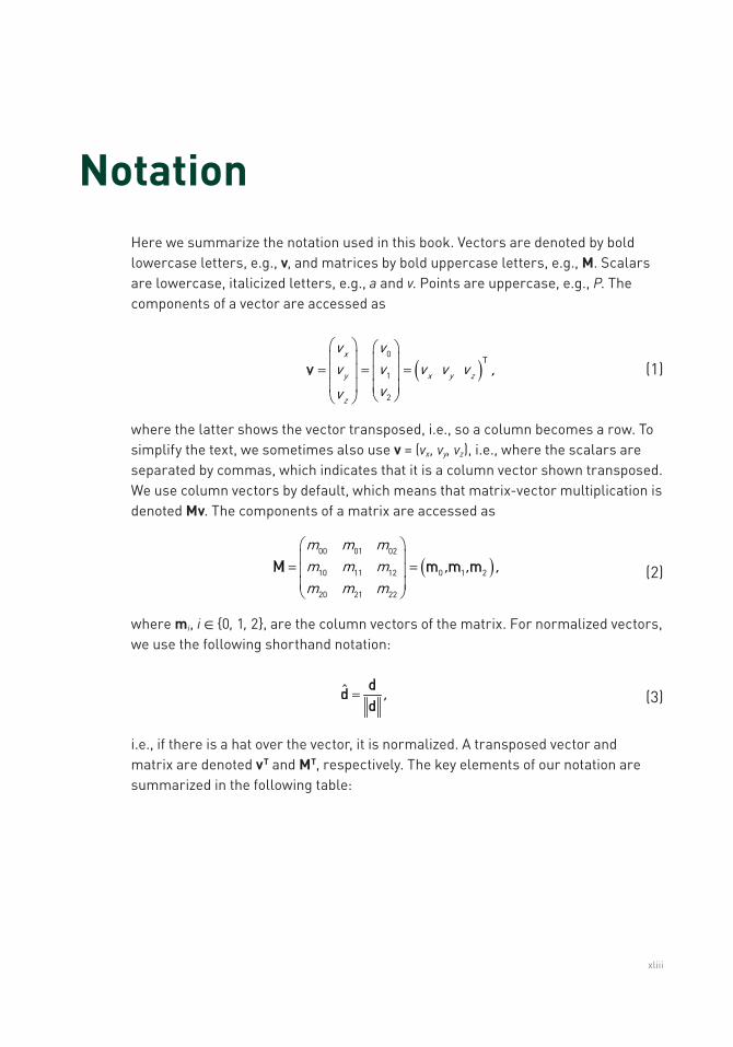
NotationHere we summarize the notation used in this book. Vectors are denoted by bold lowercase letters, e.g., v, and matrices by bold uppercase letters, e.g., M. Scalars are lowercase, italicized letters, e.g., a and v. Points are uppercase, e.g., P. The components of a vector are accessed as
( )0
1
2
x
y x y z
z
v vv v v v v ,
vv
æ ö æ öç ÷ ç ÷= = =ç ÷ ç ÷ç ÷ ç ÷
è øè ø
Tv (1)
where the latter shows the vector transposed, i.e., so a column becomes a row. To simplify the text, we sometimes also use v = (vx, vy, vz), i.e., where the scalars are separated by commas, which indicates that it is a column vector shown transposed. We use column vectors by default, which means that matrix-vector multiplication is denoted Mv. The components of a matrix are accessed as
( )00 01 02
10 11 12 0 1 2
20 21 22
m m mm m m , , ,m m m
æ öç ÷= =ç ÷ç ÷è ø
M m m m (2)
where mi, i ∈ 0, 1, 2, are the column vectors of the matrix. For normalized vectors, we use the following shorthand notation:
ˆ ,=ddd (3)
i.e., if there is a hat over the vector, it is normalized. A transposed vector and matrix are denoted vT and MT, respectively. The key elements of our notation are summarized in the following table:

xliv
Notation What It Represents
P Pointv Vectorv Normalized vectorM Matrix
A direction vector on a sphere is often denoted by ω and the entire set of directions on a (hemi)sphere is Ω. Finally, note that the cross product between two vectors is written as a × b and their dot product is a · b.
NOTATION
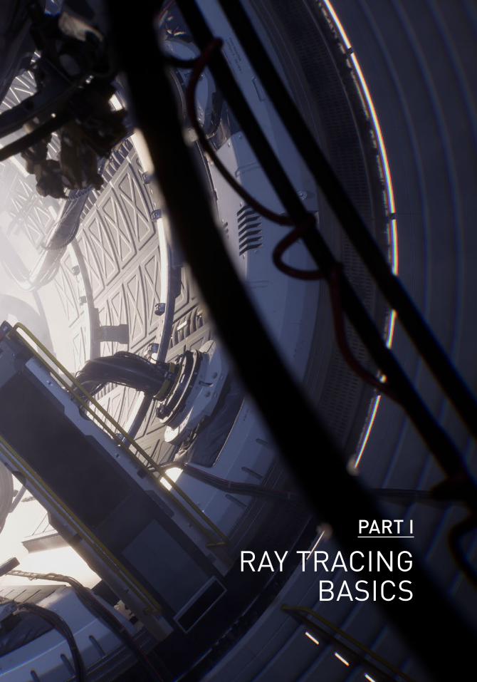
PART I
RAY TRACING BASICS
5
PART I
Ray Tracing Basics
Today, rasterization dominates real-time rendering across most application domains, so many readers looking for real-time rendering tips may have last encountered ray tracing during coursework years, possibly decades ago. This part contains various introductory chapters to help brush up on the basics, build a common vocabulary, and provide other simple (but useful) building blocks.
Chapter 1, “Ray Tracing Terminology,” defines common terms used throughout the book and references seminal research papers that introduced these ideas. For novice readers, a confusing and evolving variety of overlapping and poorly named terms awaits as you dig into the literature; reading papers from 30 years ago can be an exercise in frustration without understanding how terms evolved into those used today. This chapter provides a basic road map.
Chapter 2, “What Is a Ray?,” covers a couple common mathematical definitions of a ray, how to think about them, and which formulation is typically used for modern APIs. While a simple chapter, separating the basics of this fundamental construct may help remind readers that numerical precision issues abound. For rasterization, precision issues occur with z-fighting and shadow mapping; in ray tracing, every ray query requires care to avoid spurious intersections (more extensive coverage of precision issues comes in Chapter 6).
Recently, Microsoft introduced DirectX Raytracing, an extension to the DirectX raster API. Chapter 3, “Introduction to DirectX Raytracing,” provides a brief introduction to the abstractions, mental model, and new shader stages introduced by this programming interface. Additionally, it walks through and explains the steps needed to initialize the API and provides pointers to sample code to help get started.
Ray tracers allow trivial construction of arbitrary camera models, unlike typical raster APIs that restrict cameras to those defined by 4 × 4 projection matrices. Chapter 4, “A Planetarium Dome Master Camera,” provides the mathematics and sample code to build a ray traced camera for a 180° hemispherical dome projection, e.g., for planetariums. The chapter also demonstrates the simplicity of adding stereoscopic rendering or depth of field when using a ray tracer.

6
Chapter 5, “Computing Minima and Maxima of Subarrays,” describes three computation methods (with various computational trade-offs) for a fundamental algorithmic building block: computing the minima or maxima of arbitrary subsets of an array. On the surface, evaluating such queries is not obviously related to ray tracing, but it has applications in domains such as scientific visualization, where ray queries are commonly used.
The information in this part should help you get started with both understanding the basics of modern ray tracing and the mindset needed to efficiently render using it.
Chris Wyman
7© NVIDIA 2019 E. Haines, T. Akenine-Möller (eds.), Ray Tracing Gems, https://doi.org/10.1007/978-1-4842-4427-2_1
CHAPTER 1
Ray Tracing TerminologyEric Haines and Peter Shirley NVIDIA
ABSTRACT
This chapter provides background information and definitions for terms used throughout this book.
1.1 HISTORICAL NOTES
Ray tracing has a rich history in disciplines that track the movement of light in an environment, often referred to as radiative transfer. Graphics practitioners have imported ideas from fields such as neutron transport [2], heat transfer [6], and illumination engineering [11]. Since so many fields have studied these concepts, terminology evolves and sometimes diverges between and within disciplines. Classic papers may then appear to use terms incorrectly, which can be confusing.
The fundamental quantity of light moving along a ray is the SI unit spectral radiance, which remains constant along a ray (in a vacuum) and often behaves intuitively like the perceptual concept brightness. Before the term was standardized, spectral radiance was often called “intensity” or “brightness.” In computer graphics we usually drop “spectral,” as non-spectral radiance, a bulk quantity over all wavelengths, is never used.
Graphics-specific terminology related to rays has evolved over time. Almost all modern ray tracers are recursive and Monte Carlo; few now bother to call their renderer a “recursive Monte Carlo” ray tracer. In 1968, Appel [1] used rays to render images. In 1979, Whitted [16] and Kay and Greenberg [9] developed recursive ray tracing to depict accurate refraction and reflection. In 1982, Roth [13] used inside/outside interval lists along rays, as well as local instancing, to create renderings (and volume estimates) of CSG models.
8
In 1984, Cook et al. [4] presented distributed or distribution ray tracing. Elsewhere, this method is often called stochastic ray tracing1 to avoid confusion with distributed processing. The key insight of randomly sampling to capture effects such as depth of field, fuzzy reflections, and soft shadows is used in virtually every modern ray tracer. The next few years after 1984 saw researchers rephrasing rendering using traditional radiative transfer methods. Two important algorithms were introduced in 1986. Kajiya [8] referred to the integral transport equation as the rendering equation. He tried various solutions, including a Monte Carlo approach he named path tracing. Immel, Cohen, and Greenberg [7] wrote the same transport equation in different units and solved it with a finite element method now called radiosity.
Since the rephrasing of the graphics problem using classic transport methods three decades ago, a great deal of work has explored how to numerically solve the problem. Key algorithmic changes include the bidirectional [10, 14] and path-based [15] methods introduced in the 1990s. Many details, including how to implement these techniques in practice, are discussed in Pharr, Jakob, and Humphreys’s book [12].
1.2 DEFINITIONS
We highlight important terms used in this book. No standard set of terms exists, other than terms with standardized units, but our definitions reflect current usage in the field.
Ray casting is the process of finding the closest, or sometimes just any, object along a ray. See Chapter 2 for the definition of a ray. A ray leaves the camera through a pixel and travels until it hits the closest object. As part of shading this hit point, a new ray could be cast toward a light source to determine if the object is shadowed. See Figure 1-1.
1 The name derives from another paper by Cook [3], where he discusses using nonuniform sampling to avoid aliasing artifacts by turning them into noise.
RAY TRACING GEMS
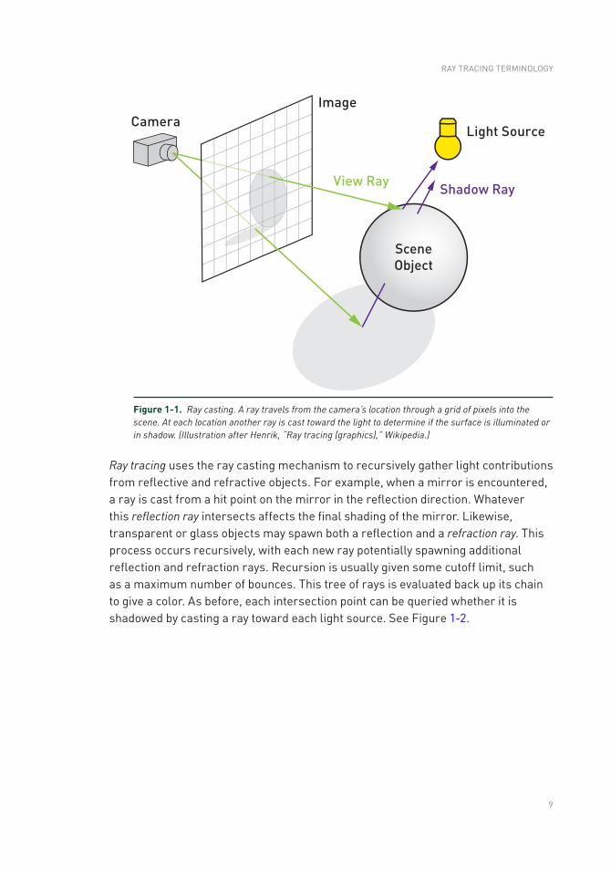
9
Ray tracing uses the ray casting mechanism to recursively gather light contributions from reflective and refractive objects. For example, when a mirror is encountered, a ray is cast from a hit point on the mirror in the reflection direction. Whatever this reflection ray intersects affects the final shading of the mirror. Likewise, transparent or glass objects may spawn both a reflection and a refraction ray. This process occurs recursively, with each new ray potentially spawning additional reflection and refraction rays. Recursion is usually given some cutoff limit, such as a maximum number of bounces. This tree of rays is evaluated back up its chain to give a color. As before, each intersection point can be queried whether it is shadowed by casting a ray toward each light source. See Figure 1-2.
Figure 1-1. Ray casting. A ray travels from the camera’s location through a grid of pixels into the scene. At each location another ray is cast toward the light to determine if the surface is illuminated or in shadow. (Illustration after Henrik, “Ray tracing (graphics),” Wikipedia.)
RAy TRACING TERMINOLOGy
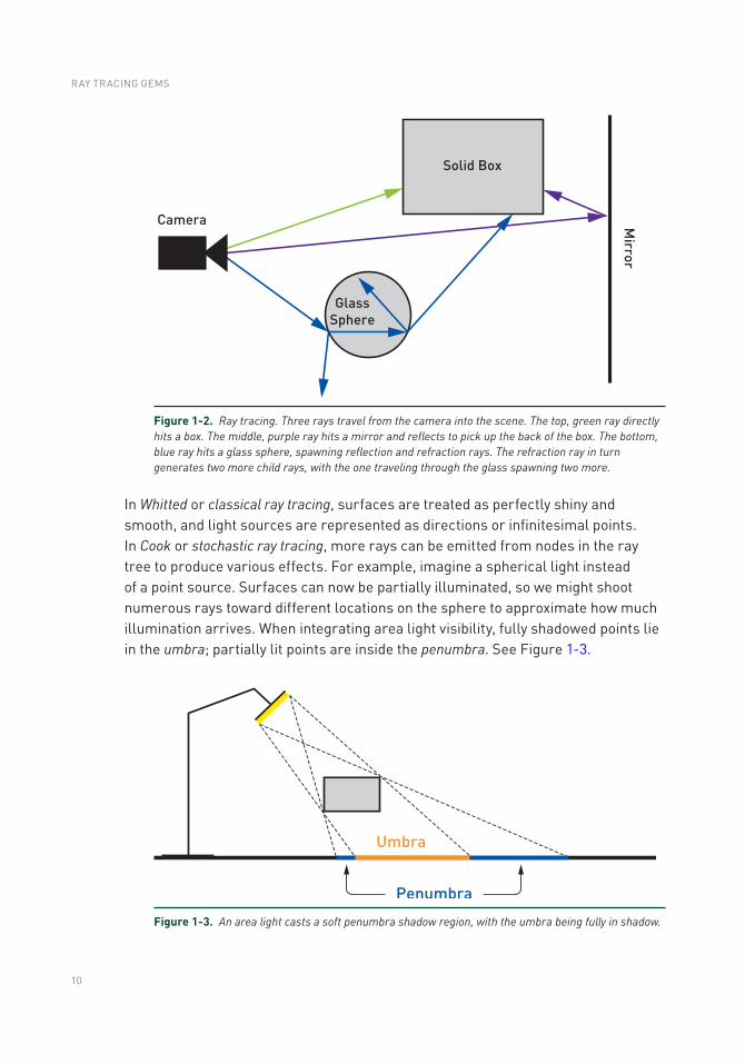
10
In Whitted or classical ray tracing, surfaces are treated as perfectly shiny and smooth, and light sources are represented as directions or infinitesimal points. In Cook or stochastic ray tracing, more rays can be emitted from nodes in the ray tree to produce various effects. For example, imagine a spherical light instead of a point source. Surfaces can now be partially illuminated, so we might shoot numerous rays toward different locations on the sphere to approximate how much illumination arrives. When integrating area light visibility, fully shadowed points lie in the umbra; partially lit points are inside the penumbra. See Figure 1-3.
Figure 1-2. Ray tracing. Three rays travel from the camera into the scene. The top, green ray directly hits a box. The middle, purple ray hits a mirror and reflects to pick up the back of the box. The bottom, blue ray hits a glass sphere, spawning reflection and refraction rays. The refraction ray in turn generates two more child rays, with the one traveling through the glass spawning two more.
Figure 1-3. An area light casts a soft penumbra shadow region, with the umbra being fully in shadow.
RAY TRACING GEMS
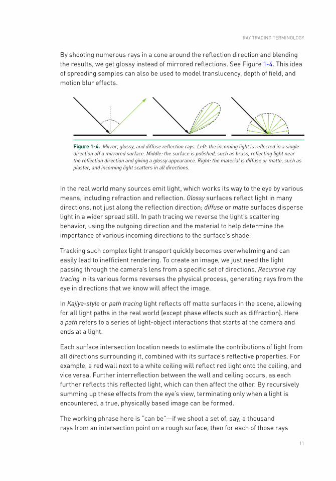
11
By shooting numerous rays in a cone around the reflection direction and blending the results, we get glossy instead of mirrored reflections. See Figure 1-4. This idea of spreading samples can also be used to model translucency, depth of field, and motion blur effects.
In the real world many sources emit light, which works its way to the eye by various means, including refraction and reflection. Glossy surfaces reflect light in many directions, not just along the reflection direction; diffuse or matte surfaces disperse light in a wider spread still. In path tracing we reverse the light’s scattering behavior, using the outgoing direction and the material to help determine the importance of various incoming directions to the surface’s shade.
Tracking such complex light transport quickly becomes overwhelming and can easily lead to inefficient rendering. To create an image, we just need the light passing through the camera’s lens from a specific set of directions. Recursive ray tracing in its various forms reverses the physical process, generating rays from the eye in directions that we know will affect the image.
In Kajiya-style or path tracing light reflects off matte surfaces in the scene, allowing for all light paths in the real world (except phase effects such as diffraction). Here a path refers to a series of light-object interactions that starts at the camera and ends at a light.
Each surface intersection location needs to estimate the contributions of light from all directions surrounding it, combined with its surface’s reflective properties. For example, a red wall next to a white ceiling will reflect red light onto the ceiling, and vice versa. Further interreflection between the wall and ceiling occurs, as each further reflects this reflected light, which can then affect the other. By recursively summing up these effects from the eye’s view, terminating only when a light is encountered, a true, physically based image can be formed.
The working phrase here is “can be”—if we shoot a set of, say, a thousand rays from an intersection point on a rough surface, then for each of those rays
Figure 1-4. Mirror, glossy, and diffuse reflection rays. Left: the incoming light is reflected in a single direction off a mirrored surface. Middle: the surface is polished, such as brass, reflecting light near the reflection direction and giving a glossy appearance. Right: the material is diffuse or matte, such as plaster, and incoming light scatters in all directions.
RAy TRACING TERMINOLOGy
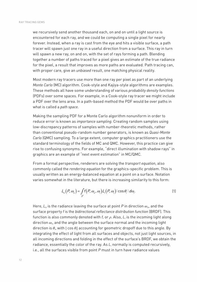
12
we recursively send another thousand each, on and on until a light source is encountered for each ray, and we could be computing a single pixel for nearly forever. Instead, when a ray is cast from the eye and hits a visible surface, a path tracer will spawn just one ray in a useful direction from a surface. This ray in turn will spawn a new ray, on and on, with the set of rays forming a path. Blending together a number of paths traced for a pixel gives an estimate of the true radiance for the pixel, a result that improves as more paths are evaluated. Path tracing can, with proper care, give an unbiased result, one matching physical reality.
Most modern ray tracers use more than one ray per pixel as part of an underlying Monte Carlo (MC) algorithm. Cook-style and Kajiya-style algorithms are examples. These methods all have some understanding of various probability density functions (PDFs) over some spaces. For example, in a Cook-style ray tracer we might include a PDF over the lens area. In a path-based method the PDF would be over paths in what is called a path space.
Making the sampling PDF for a Monte Carlo algorithm nonuniform in order to reduce error is known as importance sampling. Creating random samples using low-discrepancy patterns of samples with number-theoretic methods, rather than conventional pseudo-random number generators, is known as Quasi-Monte Carlo (QMC) sampling. To a large extent, computer graphics practitioners use the standard terminology of the fields of MC and QMC. However, this practice can give rise to confusing synonyms. For example, “direct illumination with shadow rays” in graphics are an example of “next event estimation” in MC/QMC.
From a formal perspective, renderers are solving the transport equation, also commonly called the rendering equation for the graphics-specific problem. This is usually written as an energy-balanced equation at a point on a surface. Notation varies somewhat in the literature, but there is increasing similarity to this form:
( ) ( ) ( )
S
L P, f P, , L P, d2
o o o i i i i icos .w w w w q wò= ∣ ∣
(1)
Here, Lo is the radiance leaving the surface at point P in direction ωo, and the surface property f is the bidirectional reflectance distribution function (BRDF). This function is also commonly denoted with fr or ρ. Also, Li is the incoming light along direction ωi, and the angle between the surface normal and the incoming light direction is θi, with ∣ cos θi∣ accounting for geometric dropoff due to this angle. By integrating the effect of light from all surfaces and objects, not just light sources, in all incoming directions and folding in the effect of the surface’s BRDF, we obtain the radiance, essentially the color of the ray. As Li normally is computed recursively, i.e., all the surfaces visible from point P must in turn have radiance values
RAY TRACING GEMS
13
calculated for them, path tracing and related methods are used to choose among all the possible paths, with the goal of casting each ray along the path in a direction that is significant in computing a good approximation of the effect of all possible directions.
The location point P is often left out as implicit. Also, the wavelength λ can be added as a function input. There are also more general equations that include participating media, such as smoke or fog, and physical optics effects, such as diffraction.
Related to participating media, ray marching is the process of marching along a ray by some interval, sampling it along the ray’s direction. This method of casting a ray is often used for volume rendering, where there is no specific surface. Instead, at each location the effect of light on the volume is computed by some means. An alternative to ray marching is to simulate the collisions in a volume.
Ray marching, typically under some variant of Hart’s sphere tracing algorithm [5], is also used to describe the process of intersecting a surface defined by an implicit distance equation or inside/outside test by sampling points along the ray in a search for the surface. The “sphere” in this case is a sphere of equidistant points from the surface; it has nothing to do with intersecting spheres. Following our earlier notation, this process would ideally be called “sphere casting” instead of “sphere tracing.” This type of intersection testing is commonly seen in demoscene programs and is popularized online by the Shadertoy website.
We have touched upon just the basics of ray-related rendering techniques and the terminology used. See this book’s website http://raytracinggems.com for a guide to further resources.
REFERENCES
[1] Appel, A. Some Techniques for Shading Machine Renderings of Solids. In AFIPS ’68 Spring Joint Computer Conference (1968), pp. 37–45.
[2] Arvo, J., and Kirk, D. Particle Transport and Image Synthesis. Computer Graphics (SIGGRAPH) 24, 4 (1990), 63–66.
[3] Cook, R. L. Stochastic Sampling in Computer Graphics. ACM Transactions on Graphics 5, 1 (Jan. 1986), 51–72.
[4] Cook, R. L., Porter, T., and Carpenter, L. Distributed Ray Tracing. Computer Graphics (SIGGRAPH) 18, 3 (1984), 137–145.
[5] Hart, J. C. Sphere Tracing: A Geometric Method for the Antialiased Ray Tracing of Implicit Surfaces. The Visual Computer 12, 10 (Dec 1996), 527–545.
[6] Howell, J. R., Menguc, M. P., and Siegel, R. Thermal Radiation Heat Transfer. CRC Press, 2015.
RAy TRACING TERMINOLOGy
14
[7] Immel, D. S., Cohen, M. F., and Greenberg, D. P. A Radiosity Method for Non- Diffuse Environments. Computer Graphics (SIGGRAPH) 20, 4 (Aug. 1986), 133–142.
[8] Kajiya, J. T. The Rendering Equation. Computer Graphics (SIGGRAPH) (1986), 143–150.
[9] Kay, D. S., and Greenberg, D. Transparency for Computer Synthesized Images. Computer Graphics (SIGGRAPH) 13, 2 (1979), 158–164.
[10] Lafortune, E. P. Bidirectional Path Tracing. In Compugraphics (1993), pp. 145–153.
[11] Larson, G. W., and Shakespeare, R. Rendering with Radiance: The Art and Science of Lighting Visualization. Booksurge LLC, 2004.
[12] Pharr, M., Jakob, W., and Humphreys, G. Physically Based Rendering: From Theory to Implementation, third ed. Morgan Kaufmann, 2016.
[13] Roth, S. D. Ray Casting for Modeling Solids. Computer Graphics and Image Processing 18, 2 (1982), 109–144.
[14] Veach, E., and Guibas, L. Bidirectional Estimators for Light Transport. In Photorealistic Rendering Techniques (1995), pp. 145–167.
[15] Veach, E., and Guibas, L. J. Metropolis Light Transport. In Proceedings of SIGGRAPH (1997), pp. 65–76.
[16] Whitted, T. An Improved Illumination Model for Shaded Display. Communications of the ACM 23, 6 (June 1980), 343–349.
Open Access This chapter is licensed under the terms of the Creative Commons Attribution-NonCommercial-NoDerivatives 4.0 International License (http://creativecommons.org/licenses/by-nc-nd/4.0/), which permits any noncommercial use, sharing, distribution and
reproduction in any medium or format, as long as you give appropriate credit to the original author(s) and the source, provide a link to the Creative Commons license and indicate if you modified the licensed material. you do not have permission under this license to share adapted material derived from this chapter or parts of it.
The images or other third party material in this chapter are included in the chapter's Creative Commons license, unless indicated otherwise in a credit line to the material. If material is not included in the chapter's Creative Commons license and your intended use is not permitted by statutory regulation or exceeds the permitted use, you will need to obtain permission directly from the copyright holder.
RAY TRACING GEMS
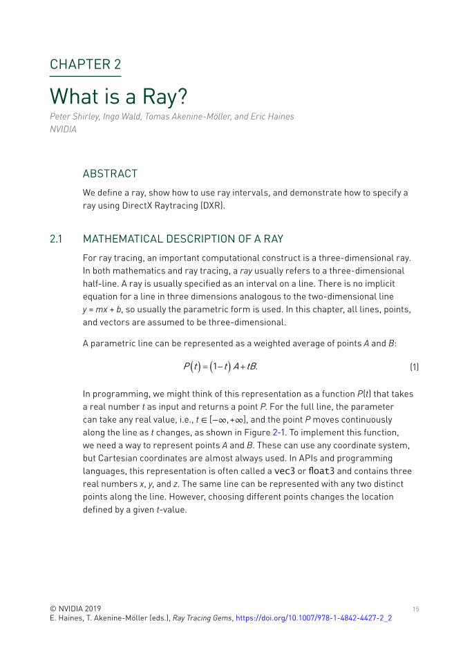
15© NVIDIA 2019 E. Haines, T. Akenine-Möller (eds.), Ray Tracing Gems, https://doi.org/10.1007/978-1-4842-4427-2_2
CHAPTER 2
What is a Ray?Peter Shirley, Ingo Wald, Tomas Akenine-Möller, and Eric Haines NVIDIA
ABSTRACT
We define a ray, show how to use ray intervals, and demonstrate how to specify a ray using DirectX Raytracing (DXR).
2.1 MATHEMATICAL DESCRIPTION OF A RAY
For ray tracing, an important computational construct is a three-dimensional ray. In both mathematics and ray tracing, a ray usually refers to a three-dimensional half-line. A ray is usually specified as an interval on a line. There is no implicit equation for a line in three dimensions analogous to the two-dimensional line y = mx + b, so usually the parametric form is used. In this chapter, all lines, points, and vectors are assumed to be three-dimensional.
A parametric line can be represented as a weighted average of points A and B:
( ) ( )P t t A tB1 .= - + (1)
In programming, we might think of this representation as a function P(t) that takes a real number t as input and returns a point P. For the full line, the parameter can take any real value, i.e., t ∈ [−∞, +∞], and the point P moves continuously along the line as t changes, as shown in Figure 2-1. To implement this function, we need a way to represent points A and B. These can use any coordinate system, but Cartesian coordinates are almost always used. In APIs and programming languages, this representation is often called a vec3 or float3 and contains three real numbers x, y, and z. The same line can be represented with any two distinct points along the line. However, choosing different points changes the location defined by a given t-value.
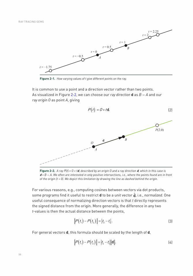
16
Figure 2-1. How varying values of t give different points on the ray.
Figure 2-2. A ray P(t) = O + td, described by an origin O and a ray direction d, which in this case is d = B − A. We often are interested in only positive intersections, i.e., where the points found are in front of the origin (t > 0). We depict this limitation by drawing the line as dashed behind the origin.
It is common to use a point and a direction vector rather than two points. As visualized in Figure 2-2, we can choose our ray direction d as B − A and our ray origin O as point A, giving
( ) .P t O t= + d (2)
For various reasons, e.g., computing cosines between vectors via dot products, some programs find it useful to restrict d to be a unit vector d, i.e., normalized. One useful consequence of normalizing direction vectors is that t directly represents the signed distance from the origin. More generally, the difference in any two t-values is then the actual distance between the points,
( ) ( )P t P t t t1 2 2 1 .- = - (3)
For general vectors d, this formula should be scaled by the length of d,
( ) ( )- = -P t P t t t1 2 2 1 .d (4)
RAY TRACING GEMS
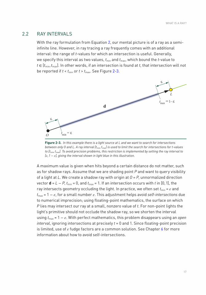
17
2.2 RAY INTERVALS
With the ray formulation from Equation 2, our mental picture is of a ray as a semi-infinite line. However, in ray tracing a ray frequently comes with an additional interval: the range of t-values for which an intersection is useful. Generally, we specify this interval as two values, tmin and tmax, which bound the t-value to t ∈ [tmin, tmax]. In other words, if an intersection is found at t, that intersection will not be reported if t < tmin or t > tmax. See Figure 2-3.
Figure 2-3. In this example there is a light source at L and we want to search for intersections between only O and L. A ray interval [tmin, tmax] is used to limit the search for intersections for t-values to [tmin, tmax]. To avoid precision problems, this restriction is implemented by setting the ray interval to [ε, 1 − ε], giving the interval shown in light blue in this illustration.
A maximum value is given when hits beyond a certain distance do not matter, such as for shadow rays. Assume that we are shading point P and want to query visibility of a light at L. We create a shadow ray with origin at O = P, unnormalized direction vector d = L − P, tmin = 0, and tmax = 1. If an intersection occurs with t in [0, 1], the ray intersects geometry occluding the light. In practice, we often set tmin = ε and tmax = 1 − ε, for a small number ε. This adjustment helps avoid self-intersections due to numerical imprecision; using floating-point mathematics, the surface on which P lies may intersect our ray at a small, nonzero value of t. For non-point lights the light’s primitive should not occlude the shadow ray, so we shorten the interval using tmax = 1 − ε. With perfect mathematics, this problem disappears using an open interval, ignoring intersections at precisely t = 0 and 1. Since floating-point precision is limited, use of ε fudge factors are a common solution. See Chapter 6 for more information about how to avoid self-intersections.
WHAT IS A RAY?
18
In implementations using normalized ray directions, we could instead use O = P,
L PL P-
=-
d , tmin = ε, and tmax = l − ε, where l = ‖L − P‖ is the distance to the light source
L. Note that this epsilon must be different than the previous epsilon, as t now has a different range.
Some renderers use unit-length vectors for all or some ray directions. Doing so allows efficient cosine computations via dot products with other unit vectors, and it can make it easier to reason about the code, in addition to making it more readable. As noted earlier, a unit length means that the ray parameter t can be interpreted as a distance without scaling by the direction vector’s length. However, instanced geometry may be represented using a transformation for each instance. Ray/object intersection then requires transforming the ray into the object’s space, which changes the length of the direction vector. To properly compute t in this new space, this transformed direction should be left unnormalized. In addition, normalization costs a little performance and can be unnecessary, as for shadow rays. Because of these competing benefits, there is no universal recommendation of whether to use unit direction vectors.
2.3 RAYS IN DXR
This section presents the definition of a ray in DirectX Raytracing [3]. In DXR, a ray is defined by the following structure:
1 struct RayDesc
2
3 float3 Origin;
4 float TMin;
5 float3 Direction;
6 float TMax;
7 ;
The ray type is handled differently in DXR, where a certain shader program is associated with each different type of ray. To trace a ray with the TraceRay() function in DXR, a RayDesc is needed. The RayDesc::Origin is set to the origin O of our ray, the RayDesc::Direction is set to the direction d, and the t-interval (RayDesc::TMin and RayDesc::TMax) must be initialized as well. For example, for an eye ray (RayDesc eyeRay) we set eyeRay.TMin = 0.0 and eyeRay.TMax = FLT_MAX, which indicates that we are interested in all intersections that are in front of the origin.
RAY TRACING GEMS
19
2.4 CONCLUSION
This chapter shows how a ray is typically defined and used in a ray tracer, and gave the DXR API’s ray definition as an example. Other ray tracing systems, such as OptiX [1] and the Vulkan ray tracing extension [2], have minor variations. For example, OptiX explicitly defines a ray type, such as a shadow ray. These systems have other commonalities, such as the idea of a ray payload. This is a data structure that can be defined by the user to carry additional information along with the ray that can be accessed and edited by separate shaders or modules. Such data is application specific. At the core, in every rendering system that defines a ray, you will find the ray’s origin, direction, and interval.
REFERENCES
[1] NVIDIA. OptiX 5.1 Programming Guide. http://raytracing-docs.nvidia.com/optix/guide/index.html, Mar. 2018.
[2] Subtil, N. Introduction to Real-Time Ray Tracing with Vulkan. NVIDIA Developer Blog, https://devblogs.nvidia.com/vulkan-raytracing/, Oct. 2018.
[3] Wyman, C., Hargreaves, S., Shirley, P., and Barré-Brisebois, C. Introduction to DirectX RayTracing. SIGGRAPH Courses, Aug. 2018.
Open Access This chapter is licensed under the terms of the Creative Commons Attribution-NonCommercial-NoDerivatives 4.0 International License (http://creativecommons.org/licenses/by-nc-nd/4.0/), which permits any noncommercial use, sharing, distribution and
reproduction in any medium or format, as long as you give appropriate credit to the original author(s) and the source, provide a link to the Creative Commons license and indicate if you modified the licensed material. You do not have permission under this license to share adapted material derived from this chapter or parts of it.
The images or other third party material in this chapter are included in the chapter's Creative Commons license, unless indicated otherwise in a credit line to the material. If material is not included in the chapter's Creative Commons license and your intended use is not permitted by statutory regulation or exceeds the permitted use, you will need to obtain permission directly from the copyright holder.
WHAT IS A RAY?
21© NVIDIA 2019 E. Haines, T. Akenine-Möller (eds.), Ray Tracing Gems, https://doi.org/10.1007/978-1-4842-4427-2_3
CHAPTER 3
Introduction to DirectX RaytracingChris Wyman and Adam Marrs NVIDIA
ABSTRACT
Modern graphics APIs such as DirectX 12 expose low-level hardware access and control to developers, often resulting in complex and verbose code that can be intimidating for novices. In this chapter, we hope to demystify the steps to set up and use DirectX for ray tracing.
3.1 INTRODUCTION
At the 2018 Game Developers Conference, Microsoft announced the DirectX Raytracing (DXR) API, which extends DirectX 12 with native support for ray tracing. Beginning with the October 2018 update to Windows 10, the API runs on all DirectX 12 GPUs, either using dedicated hardware acceleration or via a compute-based software fallback. This functionality enables new options for DirectX renderers, ranging from full-blown, film- quality path tracers to more humble ray-raster hybrids, e.g., replacing raster shadows or reflections with ray tracing.
As with all graphics APIs, a few prerequisites are important before diving into code. This chapter assumes a knowledge of ray tracing fundamentals, and we refer readers to other chapters in this book, or introductory texts [4, 10], for the basics. Additionally, we assume familiarity with GPU programming; to understand ray tracing shaders, experience with basic DirectX, Vulkan, or OpenGL helps. For lower-level details, prior experience with DirectX 12 may be beneficial.
3.2 OVERVIEW
GPU programming has three key components, independent of the API: (1) the GPU device code, (2) the CPU host-side setup process, and (3) the sharing of data between host and device. Before we discuss each of these components, Section 3.3 walks through important software and hardware requirements to get started building and running DXR-based programs.
We then talk about each core component, starting with how to code DXR shaders in Sections 3.4, 3.5, and 3.6. The high-level shading language (HLSL) code for DXR looks similar to a serial CPU ray tracer written in C++. Using libraries to abstract
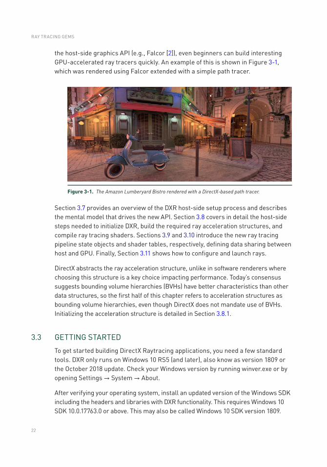
22
the host-side graphics API (e.g., Falcor [2]), even beginners can build interesting GPU-accelerated ray tracers quickly. An example of this is shown in Figure 3-1, which was rendered using Falcor extended with a simple path tracer.
Figure 3-1. The Amazon Lumberyard Bistro rendered with a DirectX-based path tracer.
Section 3.7 provides an overview of the DXR host-side setup process and describes the mental model that drives the new API. Section 3.8 covers in detail the host-side steps needed to initialize DXR, build the required ray acceleration structures, and compile ray tracing shaders. Sections 3.9 and 3.10 introduce the new ray tracing pipeline state objects and shader tables, respectively, defining data sharing between host and GPU. Finally, Section 3.11 shows how to configure and launch rays.
DirectX abstracts the ray acceleration structure, unlike in software renderers where choosing this structure is a key choice impacting performance. Today’s consensus suggests bounding volume hierarchies (BVHs) have better characteristics than other data structures, so the first half of this chapter refers to acceleration structures as bounding volume hierarchies, even though DirectX does not mandate use of BVHs. Initializing the acceleration structure is detailed in Section 3.8.1.
3.3 GETTING STARTED
To get started building DirectX Raytracing applications, you need a few standard tools. DXR only runs on Windows 10 RS5 (and later), also know as version 1809 or the October 2018 update. Check your Windows version by running winver.exe or by opening Settings → System → About.
After verifying your operating system, install an updated version of the Windows SDK including the headers and libraries with DXR functionality. This requires Windows 10 SDK 10.0.17763.0 or above. This may also be called Windows 10 SDK version 1809.
RAY TRACING GEMS
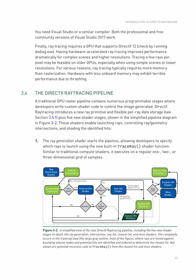
23
You need Visual Studio or a similar compiler. Both the professional and free community versions of Visual Studio 2017 work.
Finally, ray tracing requires a GPU that supports DirectX 12 (check by running dxdiag.exe). Having hardware-accelerated ray tracing improves performance dramatically for complex scenes and higher resolutions. Tracing a few rays per pixel may be feasible on older GPUs, especially when using simple scenes or lower resolutions. For various reasons, ray tracing typically requires more memory than rasterization. Hardware with less onboard memory may exhibit terrible performance due to thrashing.
3.4 THE DIRECTX RAYTRACING PIPELINE
A traditional GPU raster pipeline contains numerous programmable stages where developers write custom shader code to control the image generated. DirectX Raytracing introduces a new ray primitive and flexible per-ray data storage (see Section 3.5.1) plus five new shader stages, shown in the simplified pipeline diagram in Figure 3-2. These shaders enable launching rays, controlling ray/geometry intersections, and shading the identified hits:
1. The ray generation shader starts the pipeline, allowing developers to specify which rays to launch using the new built-in TraceRay() shader function. Similar to traditional compute shaders, it executes on a regular one-, two-, or three-dimensional grid of samples.
Figure 3-2. A simplified view of the new DirectX Raytracing pipeline, including the five new shader stages (in blue): the ray generation, intersection, any-hit, closest-hit, and miss shaders. The complexity occurs in the traversal loop (the large gray outline, most of the figure), where rays are tested against bounding volume nodes and potential hits are identified and ordered to determine the closest hit. Not shown are potential recursive calls to TraceRay() from the closest-hit and miss shaders.
INTRODUCTION TO DIRECTX RAYTRACING
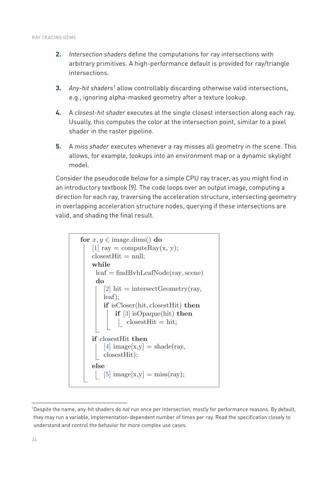
24
2. Intersection shaders define the computations for ray intersections with arbitrary primitives. A high-performance default is provided for ray/triangle intersections.
3. Any-hit shaders1 allow controllably discarding otherwise valid intersections, e.g., ignoring alpha-masked geometry after a texture lookup.
4. A closest-hit shader executes at the single closest intersection along each ray. Usually, this computes the color at the intersection point, similar to a pixel shader in the raster pipeline.
5. A miss shader executes whenever a ray misses all geometry in the scene. This allows, for example, lookups into an environment map or a dynamic skylight model.
Consider the pseudocode below for a simple CPU ray tracer, as you might find in an introductory textbook [9]. The code loops over an output image, computing a direction for each ray, traversing the acceleration structure, intersecting geometry in overlapping acceleration structure nodes, querying if these intersections are valid, and shading the final result.
1 Despite the name, any-hit shaders do not run once per intersection, mostly for performance reasons. By default, they may run a variable, implementation-dependent number of times per ray. Read the specification closely to understand and control the behavior for more complex use cases.
RAY TRACING GEMS
25
At least for standard use cases, the new DXR shaders have correspondences with parts of this simple ray tracer. The launch size of the ray generation shader corresponds to the image dimensions. Camera computations to generate each pixel’s ray occur in the ray generation shader.
While a ray traverses the bounding volume hierarchy, actual intersections of primitives in the leaf node logically occur in DirectX intersection shaders, and detected intersections can be discarded in the any-hit shader. Finally, once a ray has completed its traversal through the acceleration structure, it is either shaded in the closest-hit shader or given a default color in the miss shader.
3.5 NEW HLSL SUPPORT FOR DIRECTX RAYTRACING
Augmenting the standard HLSL data types, texture and buffer resources, and built- in functions (see the DirectX documentation [5]), Microsoft added various built-in intrinsics to support the functionality needed for ray tracing. New intrinsic functions fall into five categories:
1. Ray traversal functions spawn rays and allow control of their execution.
2. Launch introspection functions query launch dimensions and identify which ray (or pixel) the current thread is processing. These functions are valid in any ray tracing shader.
3. Ray introspection functions query ray parameters and properties and are available whenever you have an input ray (all ray tracing shaders except the ray generation shader).
4. Object introspection functions query object and instance properties and are usable whenever you have an input primitive (intersection, any-hit, and closest-hit shaders).
5. Hit introspection functions query properties of the current intersection. Properties are largely user defined, so these functions allow communication between intersection and hit shaders. These functions are available only during any-hit and closest-hit shaders.
3.5.1 LAUNCHING A NEW RAY IN HLSL
The most important new function, TraceRay(), launches a ray. Logically, this behaves akin to a texture fetch: it pauses your shader for a variable (and potentially large) number of GPU clocks, resuming execution when results are available
INTRODUCTION TO DIRECTX RAYTRACING
26
for further processing. Ray generation, closest-hit, and miss shaders can call TraceRay(). These shaders can launch zero, one, or many rays per thread. The code for a basic ray launch looks as follows:
1 RaytracingAccelerationStructure scene; // Scene BVH from C++
2 RayDesc ray = rayOrigin, minHitDist, rayDirection, maxHitDist ;
3 UserDefinedPayloadStruct payload = ... <initialize here>... ;
4
5 TraceRay( scene, RAY_FLAG_NONE, instancesToQuery, // What geometry?
6 hitGroup, numHitGroups, missShader, // Which shaders?
7 ray, // What ray to trace?
8 payload ); // What data to use?
The user-defined payload structure contains per-ray data persistent over a ray’s lifetime. Use it to maintain ray state during traversal and return results from TraceRay(). DirectX defines the RayDesc structure to store ray origin, direction, and minimum and maximum hit distances (ordered to pack in two float4s). Ray intersections outside the specified interval are ignored. The acceleration structure is defined via the host API (see Section 3.8.1).
The first TraceRay() parameter selects the BVH containing your geometry. Simple ray tracers often use a single BVH, but independently querying multiple structures can allow varying behavior for different geometry classes (e.g., transparent/opaque, dynamic/static). The second parameter contains flags that alter ray behavior, e.g., specifying additional optimizations valid on the ray. The third parameter is an integer instance mask that allows skipping geometry based on per-instance bitmasks; this should be 0xFF to test all geometry.
The fourth and fifth parameters help select which hit group to use. A hit group consists of an intersection, closest-hit, and any-hit shader (some of which may be null). Which set is used depends on these parameters and what geometry type and BVH instance are tested. For basic ray tracers, there is typically one hit group per ray type: for example, primary rays might use hit group 0, shadow rays use hit group 1, and global illumination rays use hit group 2. In that case, the fourth parameter selects the ray type and the fifth specifies the number of different types.
The sixth parameter specifies which miss shader to use. This simply indexes into the list of miss shaders loaded. The seventh parameter is the ray to trace, and the eighth parameter should be this ray’s user-defined persistent payload structure.
RAY TRACING GEMS
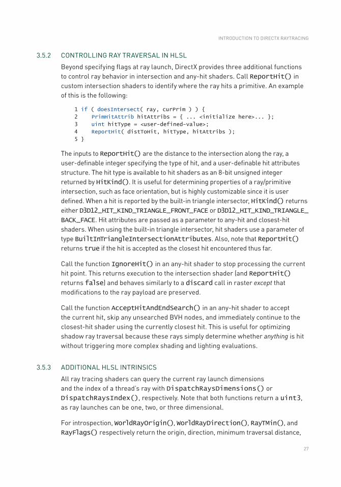
27
3.5.2 CONTROLLING RAY TRAVERSAL IN HLSL
Beyond specifying flags at ray launch, DirectX provides three additional functions to control ray behavior in intersection and any-hit shaders. Call ReportHit() in custom intersection shaders to identify where the ray hits a primitive. An example of this is the following:
1 if ( doesIntersect( ray, curPrim ) )
2 PrimHitAttrib hitAttribs = ... <initialize here>... ;
3 uint hitType = <user-defined-value>;
4 ReportHit( distToHit, hitType, hitAttribs );
5
The inputs to ReportHit() are the distance to the intersection along the ray, a user-definable integer specifying the type of hit, and a user-definable hit attributes structure. The hit type is available to hit shaders as an 8-bit unsigned integer returned by HitKind(). It is useful for determining properties of a ray/primitive intersection, such as face orientation, but is highly customizable since it is user defined. When a hit is reported by the built-in triangle intersector, HitKind() returns either D3D12_HIT_KIND_TRIANGLE_FRONT_FACE or D3D12_HIT_KIND_TRIANGLE_BACK_FACE. Hit attributes are passed as a parameter to any-hit and closest-hit shaders. When using the built-in triangle intersector, hit shaders use a parameter of type BuiltInTriangleIntersectionAttributes. Also, note that ReportHit() returns true if the hit is accepted as the closest hit encountered thus far.
Call the function IgnoreHit() in an any-hit shader to stop processing the current hit point. This returns execution to the intersection shader (and ReportHit() returns false) and behaves similarly to a discard call in raster except that modifications to the ray payload are preserved.
Call the function AcceptHitAndEndSearch() in an any-hit shader to accept the current hit, skip any unsearched BVH nodes, and immediately continue to the closest-hit shader using the currently closest hit. This is useful for optimizing shadow ray traversal because these rays simply determine whether anything is hit without triggering more complex shading and lighting evaluations.
3.5.3 ADDITIONAL HLSL INTRINSICS
All ray tracing shaders can query the current ray launch dimensions and the index of a thread’s ray with DispatchRaysDimensions() or DispatchRaysIndex(), respectively. Note that both functions return a uint3, as ray launches can be one, two, or three dimensional.
For introspection, WorldRayOrigin(), WorldRayDirection(), RayTMin(), and RayFlags() respectively return the origin, direction, minimum traversal distance,
INTRODUCTION TO DIRECTX RAYTRACING
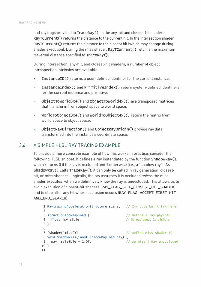
28
and ray flags provided to TraceRay(). In the any-hit and closest-hit shaders, RayTCurrent() returns the distance to the current hit. In the intersection shader, RayTCurrent() returns the distance to the closest hit (which may change during shader execution). During the miss shader, RayTCurrent() returns the maximum traversal distance specified to TraceRay().
During intersection, any-hit, and closest-hit shaders, a number of object introspection intrinsics are available:
> InstanceID() returns a user-defined identifier for the current instance.
> InstanceIndex() and PrimitiveIndex() return system-defined identifiers for the current instance and primitive.
> ObjectToWorld3x4() and ObjectToWorld4x3() are transposed matrices that transform from object space to world space.
> WorldToObject3x4() and WorldToObject4x3() return the matrix from world space to object space.
> ObjectRayDirection() and ObjectRayOrigin() provide ray data transformed into the instance’s coordinate space.
3.6 A SIMPLE HLSL RAY TRACING EXAMPLE
To provide a more concrete example of how this works in practice, consider the following HLSL snippet. It defines a ray instantiated by the function ShadowRay(), which returns 0 if the ray is occluded and 1 otherwise (i.e., a “shadow ray”). As ShadowRay() calls TraceRay(), it can only be called in ray generation, closest-hit, or miss shaders. Logically, the ray assumes it is occluded unless the miss shader executes, when we definitively know the ray is unoccluded. This allows us to avoid execution of closest-hit shaders (RAY_FLAG_SKIP_CLOSEST_HIT_SHADER) and to stop after any hit where occlusion occurs (RAY_FLAG_ACCEPT_FIRST_HIT_AND_END_SEARCH).
1 RaytracingAccelerationStructure scene; // C++ puts built BVH here
2
3 struct ShadowPayload // Define a ray payload
4 float isVisible; // 0: occluded, 1: visible
5 ;
6
7 [shader("miss")] // Define miss shader #0
8 void ShadowMiss(inout ShadowPayload pay)
9 pay.isVisible = 1.0f; // We miss ! Ray unoccluded
10
11
RAY TRACING GEMS
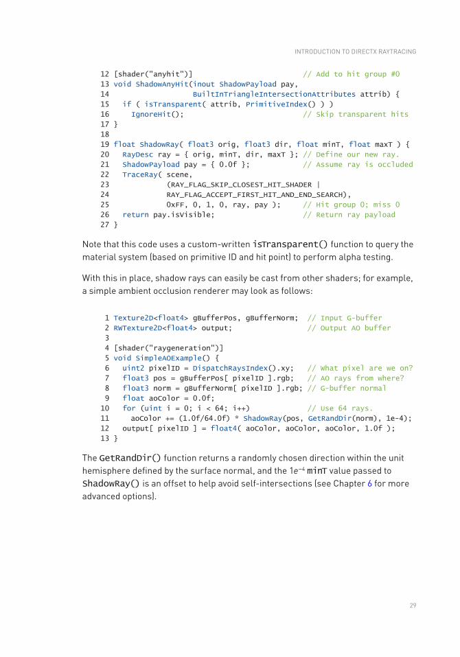
29
12 [shader("anyhit")] // Add to hit group #0
13 void ShadowAnyHit(inout ShadowPayload pay,
14 BuiltInTriangleIntersectionAttributes attrib)
15 if ( isTransparent( attrib, PrimitiveIndex() ) )
16 IgnoreHit(); // Skip transparent hits
17
18
19 float ShadowRay( float3 orig, float3 dir, float minT, float maxT )
20 RayDesc ray = orig, minT, dir, maxT ; // Define our new ray.
21 ShadowPayload pay = 0.0f ; // Assume ray is occluded
22 TraceRay( scene,
23 (RAY_FLAG_SKIP_CLOSEST_HIT_SHADER |
24 RAY_FLAG_ACCEPT_FIRST_HIT_AND_END_SEARCH),
25 0xFF, 0, 1, 0, ray, pay ); // Hit group 0; miss 0
26 return pay.isVisible; // Return ray payload
27
Note that this code uses a custom-written isTransparent() function to query the material system (based on primitive ID and hit point) to perform alpha testing.
With this in place, shadow rays can easily be cast from other shaders; for example, a simple ambient occlusion renderer may look as follows:
1 Texture2D<float4> gBufferPos, gBufferNorm; // Input G-buffer
2 RWTexture2D<float4> output; // Output AO buffer
3
4 [shader("raygeneration")]
5 void SimpleAOExample()
6 uint2 pixelID = DispatchRaysIndex().xy; // What pixel are we on?
7 float3 pos = gBufferPos[ pixelID ].rgb; // AO rays from where?
8 float3 norm = gBufferNorm[ pixelID ].rgb; // G-buffer normal
9 float aoColor = 0.0f;
10 for (uint i = 0; i < 64; i++) // Use 64 rays.
11 aoColor += (1.0f/64.0f) * ShadowRay(pos, GetRandDir(norm), 1e-4);
12 output[ pixelID ] = float4( aoColor, aoColor, aoColor, 1.0f );
13
The GetRandDir() function returns a randomly chosen direction within the unit hemisphere defined by the surface normal, and the 1e−4 minT value passed to ShadowRay() is an offset to help avoid self-intersections (see Chapter 6 for more advanced options).
INTRODUCTION TO DIRECTX RAYTRACING

30
3.7 OVERVIEW OF HOST INITIALIZATION FOR DIRECTX RAYTRACING
Until now, we focused on the shader code necessary for DirectX Raytracing. If using an engine or framework supporting DXR, this should provide enough to get started. However, when starting from scratch, you also need some low-level DirectX host-side code to initialize your ray tracer. Detailed in Sections 3.8–3.11, key initialization steps include:
1. Initialize a DirectX device and verify that it supports ray tracing.
2. Build a ray acceleration structure and specify your scene geometry.
3. Load and compile your shaders.
4. Define root signatures and shader tables to pass rendering parameters from the CPU to GPU.
5. Define DirectX pipeline state objects for your ray tracing pipeline.
6. Dispatch work to the GPU to actually trace the rays.
As with all DirectX 12 APIs, the ray tracing API is low level and verbose. Even simple samples [3] run over 1000 lines of C++ code after allocating all resources, performing validation, and checking for errors. For clarity and brevity, our code snippets in the following sections focus on new key functions and structures needed for ray tracing.
3.7.1 INSIGHT INTO THE MENTAL MODEL
When trying to understand these code snippets, remember the goals. Unlike rasterization, when ray tracing each ray may intersect arbitrary geometry and materials. Allowing for this flexibility while also achieving high performance means making available shader data for all potentially intersected surfaces on the GPU in a well- organized and easily indexable format. As a result, the process of tracing rays and shading intersected surfaces are coupled in DirectX, unlike offline or CPU ray tracers where these two operations are often independent.
Consider the new shader stages in Section 3.4. Ray generation shaders have a standard GPU programming model, where groups of threads launch in parallel, but the other shader programs effectively act as callbacks: run one when a ray hits a sphere, run another to shade a point on a triangle, and run a third when missing all geometry. Shaders get spawned, wake up, and need to identify work to perform without the benefit of a continuous execution history. If a spawned shader’s work depends on geometric properties, DirectX needs to understand this relationship, e.g., closest-hit shading may depend on a surface normal computed during intersection.
RAY TRACING GEMS
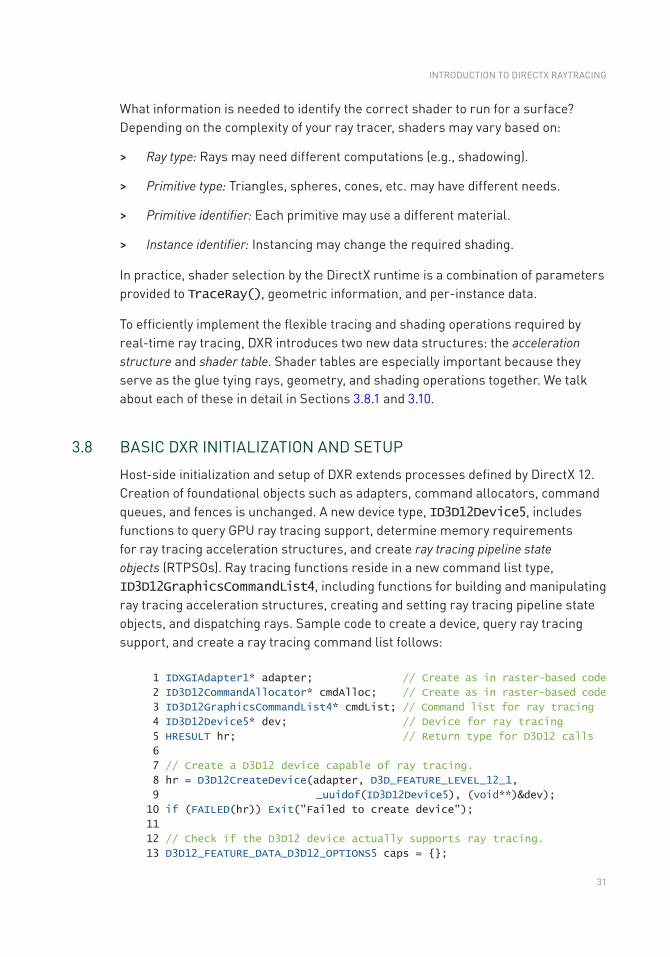
31
What information is needed to identify the correct shader to run for a surface? Depending on the complexity of your ray tracer, shaders may vary based on:
> Ray type: Rays may need different computations (e.g., shadowing).
> Primitive type: Triangles, spheres, cones, etc. may have different needs.
> Primitive identifier: Each primitive may use a different material.
> Instance identifier: Instancing may change the required shading.
In practice, shader selection by the DirectX runtime is a combination of parameters provided to TraceRay(), geometric information, and per-instance data.
To efficiently implement the flexible tracing and shading operations required by real- time ray tracing, DXR introduces two new data structures: the acceleration structure and shader table. Shader tables are especially important because they serve as the glue tying rays, geometry, and shading operations together. We talk about each of these in detail in Sections 3.8.1 and 3.10.
3.8 BASIC DXR INITIALIZATION AND SETUP
Host-side initialization and setup of DXR extends processes defined by DirectX 12. Creation of foundational objects such as adapters, command allocators, command queues, and fences is unchanged. A new device type, ID3D12Device5, includes functions to query GPU ray tracing support, determine memory requirements for ray tracing acceleration structures, and create ray tracing pipeline state objects (RTPSOs). Ray tracing functions reside in a new command list type, ID3D12GraphicsCommandList4, including functions for building and manipulating ray tracing acceleration structures, creating and setting ray tracing pipeline state objects, and dispatching rays. Sample code to create a device, query ray tracing support, and create a ray tracing command list follows:
1 IDXGIAdapter1* adapter; // Create as in raster-based code
2 ID3D12CommandAllocator* cmdAlloc; // Create as in raster-based code
3 ID3D12GraphicsCommandList4* cmdList; // Command list for ray tracing
4 ID3D12Device5* dev; // Device for ray tracing
5 HRESULT hr; // Return type for D3D12 calls
6
7 // Create a D3D12 device capable of ray tracing.
8 hr = D3D12CreateDevice(adapter, D3D_FEATURE_LEVEL_12_1,
9 _uuidof(ID3D12Device5), (void**)&dev);
10 if (FAILED(hr)) Exit("Failed to create device");
11
12 // Check if the D3D12 device actually supports ray tracing.
13 D3D12_FEATURE_DATA_D3D12_OPTIONS5 caps = ;
INTRODUCTION TO DIRECTX RAYTRACING
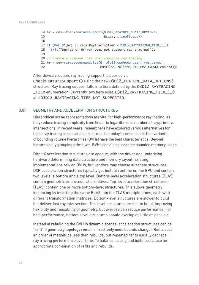
32
14 hr = dev->CheckFeatureSupport(D3D12_FEATURE_D3D12_OPTIONS5,
15 &caps, sizeof(caps));
16
17 if (FAILED(hr) || caps.RaytracingTier < D3D12_RAYTRACING_TIER_1_0)
18 Exit("Device or driver does not support ray tracing!");
19
20 // Create a command list that supports ray tracing.
21 hr = dev->CreateCommandList(0, D3D12_COMMAND_LIST_TYPE_DIRECT,
22 cmdAlloc, nullptr, IID_PPV_ARGS(& cmdList));
After device creation, ray tracing support is queried via CheckFeatureSupport() using the new D3D12_FEATURE_DATA_OPTIONS5 structure. Ray tracing support falls into tiers defined by the D3D12_RAYTRACING _TIER enumeration. Currently, two tiers exist: D3D12_RAYTRACING_TIER_1_0 and D3D12_RAYTRACING_TIER_NOT_SUPPORTED.
3.8.1 GEOMETRY AND ACCELERATION STRUCTURES
Hierarchical scene representations are vital for high-performance ray tracing, as they reduce tracing complexity from linear to logarithmic in number of ray/primitive intersections. In recent years, researchers have explored various alternatives for these ray tracing acceleration structures, but today’s consensus is that variants of bounding volume hierarchies (BVHs) have the best characteristics. Beyond hierarchically grouping primitives, BVHs can also guarantee bounded memory usage.
DirectX acceleration structures are opaque, with the driver and underlying hardware determining data structure and memory layout. Existing implementations rely on BVHs, but vendors may choose alternate structures. DXR acceleration structures typically get built at runtime on the GPU and contain two levels: a bottom and a top level. Bottom- level acceleration structures (BLAS) contain geometric or procedural primitives. Top- level acceleration structures (TLAS) contain one or more bottom-level structures. This allows geometry instancing by inserting the same BLAS into the TLAS multiple times, each with different transformation matrices. Bottom-level structures are slower to build but deliver fast ray intersection. Top-level structures are fast to build, improving flexibility and reusability of geometry, but overuse can reduce performance. For best performance, bottom-level structures should overlap as little as possible.
Instead of rebuilding the BVH in dynamic scenes, acceleration structures can be “refit” if geometry topology remains fixed (only node bounds change). Refits cost an order of magnitude less than rebuilds, but repeated refits usually degrade ray tracing performance over time. To balance tracing and build costs, use an appropriate combination of refits and rebuilds.
RAY TRACING GEMS
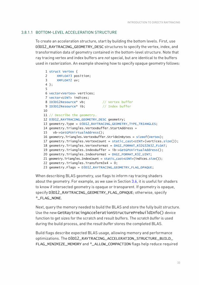
33
3.8.1.1 BOTTOM-LEVEL ACCELERATION STRUCTURE
To create an acceleration structure, start by building the bottom levels. First, use D3D12_RAYTRACING_GEOMETRY_DESC structures to specify the vertex, index, and transformation data of geometry contained in the bottom-level structure. Note that ray tracing vertex and index buffers are not special, but are identical to the buffers used in rasterization. An example showing how to specify opaque geometry follows:
1 struct Vertex
2 XMFLOAT3 position;
3 XMFLOAT2 uv;
4 ;
5
6 vector<Vertex> vertices;
7 vector<UINT> indices;
8 ID3D12Resource* vb; // Vertex buffer
9 ID3D12Resource* ib; // Index buffer
10
11 // Describe the geometry.
12 D3D12_RAYTRACING_GEOMETRY_DESC geometry;
13 geometry.Type = D3D12_RAYTRACING_GEOMETRY_TYPE_TRIANGLES;
14 geometry.Triangles.VertexBuffer.StartAddress =
15 vb->GetGPUVirtualAddress();
16 geometry.Triangles.VertexBuffer.StrideInBytes = sizeof(Vertex);
17 geo metry.Triangles.VertexCount = static_cast<UINT>(vertices.size());
18 geometry.Triangles.VertexFormat = DXGI_FORMAT_R32G32B32_FLOAT;
19 geometry.Triangles.IndexBuffer = ib->GetGPUVirtualAddress();
20 geometry.Triangles.IndexFormat = DXGI_FORMAT_R32_UINT;
21 geometry.Triangles.IndexCount = static_cast<UINT>(indices.size());
22 geometry.Triangles.Transform3x4 = 0;
23 geometry.Flags = D3D12_RAYTRACING_GEOMETRY_FLAG_OPAQUE;
When describing BLAS geometry, use flags to inform ray tracing shaders about the geometry. For example, as we saw in Section 3.6, it is useful for shaders to know if intersected geometry is opaque or transparent. If geometry is opaque, specify D3D12_RAYTRACING_GEOMETRY_FLAG_OPAQUE; otherwise, specify *_FLAG_NONE.
Next, query the memory needed to build the BLAS and store the fully built structure. Use the new GetRaytracingAccelerationStructurePrebuildInfo() device function to get sizes for the scratch and result buffers. The scratch buffer is used during the build process, and the result buffer stores the completed BLAS.
Build flags describe expected BLAS usage, allowing memory and performance optimizations. The D3D12_RAYTRACING_ACCELERATION_STRUCTURE_BUILD_FLAG_MINIMIZE_MEMORY and *_ALLOW_COMPACTION flags help reduce required
INTRODUCTION TO DIRECTX RAYTRACING
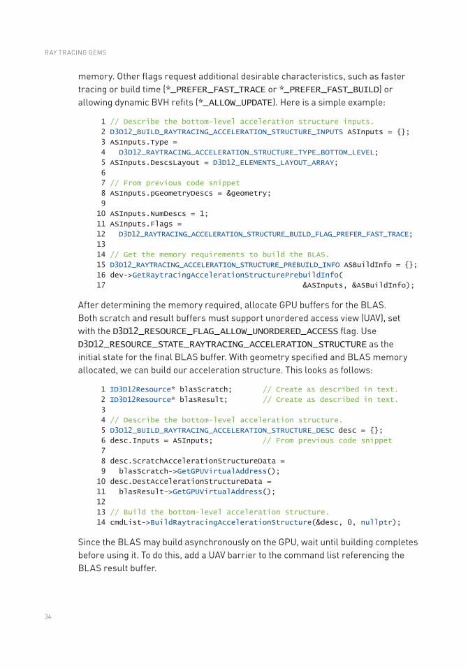
34
memory. Other flags request additional desirable characteristics, such as faster tracing or build time (*_PREFER_FAST_TRACE or *_PREFER_FAST_BUILD) or allowing dynamic BVH refits (*_ALLOW_UPDATE). Here is a simple example:
1 // Describe the bottom-level acceleration structure inputs.
2 D3D12_BUILD_RAYTRACING_ACCELERATION_STRUCTURE_INPUTS ASInputs = ;
3 ASInputs.Type =
4 D3D12_RAYTRACING_ACCELERATION_STRUCTURE_TYPE_BOTTOM_LEVEL;
5 ASInputs.DescsLayout = D3D12_ELEMENTS_LAYOUT_ARRAY;
6
7 // From previous code snippet
8 ASInputs.pGeometryDescs = &geometry;
9
10 ASInputs.NumDescs = 1;
11 ASInputs.Flags =
12 D3D12_RAYTRACING_ACCELERATION_STRUCTURE_BUILD_FLAG_PREFER_FAST_TRACE;
13
14 // Get the memory requirements to build the BLAS.
15 D3D12_RAYTRACING_ACCELERATION_STRUCTURE_PREBUILD_INFO ASBuildInfo = ;
16 dev->GetRaytracingAccelerationStructurePrebuildInfo(
17 &ASInputs, &ASBuildInfo);
After determining the memory required, allocate GPU buffers for the BLAS. Both scratch and result buffers must support unordered access view (UAV), set with the D3D12_RESOURCE_FLAG_ALLOW_UNORDERED_ACCESS flag. Use D3D12_RESOURCE_STATE_RAYTRACING_ACCELERATION_STRUCTURE as the initial state for the final BLAS buffer. With geometry specified and BLAS memory allocated, we can build our acceleration structure. This looks as follows:
1 ID3D12Resource* blasScratch; // Create as described in text.
2 ID3D12Resource* blasResult; // Create as described in text.
3
4 // Describe the bottom-level acceleration structure.
5 D3D12_BUILD_RAYTRACING_ACCELERATION_STRUCTURE_DESC desc = ;
6 desc.Inputs = ASInputs; // From previous code snippet
7
8 desc.ScratchAccelerationStructureData =
9 blasScratch->GetGPUVirtualAddress();
10 desc.DestAccelerationStructureData =
11 blasResult->GetGPUVirtualAddress();
12
13 // Build the bottom-level acceleration structure.
14 cmdList->BuildRaytracingAccelerationStructure(&desc, 0, nullptr);
Since the BLAS may build asynchronously on the GPU, wait until building completes before using it. To do this, add a UAV barrier to the command list referencing the BLAS result buffer.
RAY TRACING GEMS
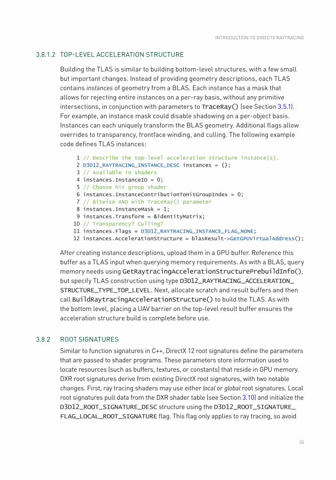
35
3.8.1.2 TOP-LEVEL ACCELERATION STRUCTURE
Building the TLAS is similar to building bottom-level structures, with a few small but important changes. Instead of providing geometry descriptions, each TLAS contains instances of geometry from a BLAS. Each instance has a mask that allows for rejecting entire instances on a per-ray basis, without any primitive intersections, in conjunction with parameters to TraceRay() (see Section 3.5.1). For example, an instance mask could disable shadowing on a per-object basis. Instances can each uniquely transform the BLAS geometry. Additional flags allow overrides to transparency, frontface winding, and culling. The following example code defines TLAS instances:
1 // Describe the top-level acceleration structure instance(s).
2 D3D12_RAYTRACING_INSTANCE_DESC instances = ;
3 // Available in shaders
4 instances.InstanceID = 0;
5 // Choose hit group shader
6 instances.InstanceContributionToHitGroupIndex = 0;
7 // Bitwise AND with TraceRay() parameter
8 instances.InstanceMask = 1;
9 instances.Transform = &identityMatrix;
10 // Transparency? Culling?
11 instances.Flags = D3D12_RAYTRACING_INSTANCE_FLAG_NONE;
12 instances.AccelerationStructure = blasResult->GetGPUVirtualAddress();
After creating instance descriptions, upload them in a GPU buffer. Reference this buffer as a TLAS input when querying memory requirements. As with a BLAS, query memory needs using GetRaytracingAccelerationStructurePrebuildInfo(), but specify TLAS construction using type D3D12_RAYTRACING_ACCELERATION_STRUCTURE_TYPE_TOP_LEVEL. Next, allocate scratch and result buffers and then call BuildRaytracingAccelerationStructure() to build the TLAS. As with the bottom level, placing a UAV barrier on the top-level result buffer ensures the acceleration structure build is complete before use.
3.8.2 ROOT SIGNATURES
Similar to function signatures in C++, DirectX 12 root signatures define the parameters that are passed to shader programs. These parameters store information used to locate resources (such as buffers, textures, or constants) that reside in GPU memory. DXR root signatures derive from existing DirectX root signatures, with two notable changes. First, ray tracing shaders may use either local or global root signatures. Local root signatures pull data from the DXR shader table (see Section 3.10) and initialize the D3D12_ROOT_SIGNATURE_DESC structure using the D3D12_ROOT_SIGNATURE_FLAG_LOCAL_ROOT_SIGNATURE flag. This flag only applies to ray tracing, so avoid
INTRODUCTION TO DIRECTX RAYTRACING
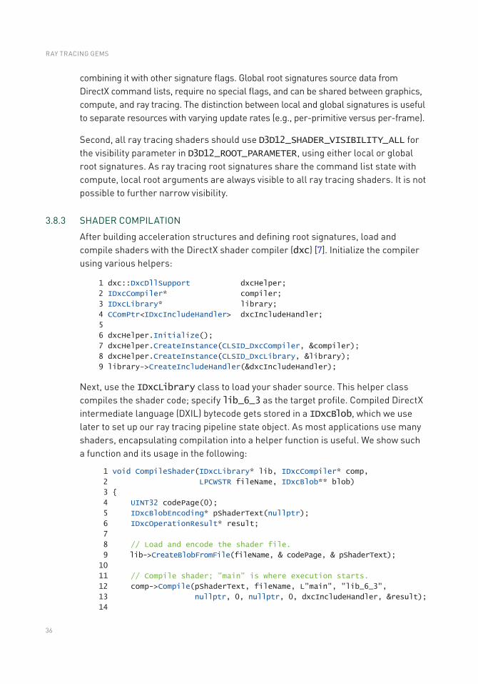
36
combining it with other signature flags. Global root signatures source data from DirectX command lists, require no special flags, and can be shared between graphics, compute, and ray tracing. The distinction between local and global signatures is useful to separate resources with varying update rates (e.g., per-primitive versus per-frame).
Second, all ray tracing shaders should use D3D12_SHADER_VISIBILITY_ALL for the visibility parameter in D3D12_ROOT_PARAMETER, using either local or global root signatures. As ray tracing root signatures share the command list state with compute, local root arguments are always visible to all ray tracing shaders. It is not possible to further narrow visibility.
3.8.3 SHADER COMPILATION
After building acceleration structures and defining root signatures, load and compile shaders with the DirectX shader compiler (dxc) [7]. Initialize the compiler using various helpers:
1 dxc::DxcDllSupport dxcHelper;
2 IDxcCompiler* compiler;
3 IDxcLibrary* library;
4 CComPtr<IDxcIncludeHandler> dxcIncludeHandler;
5
6 dxcHelper.Initialize();
7 dxcHelper.CreateInstance(CLSID_DxcCompiler, &compiler);
8 dxcHelper.CreateInstance(CLSID_DxcLibrary, &library);
9 library->CreateIncludeHandler(&dxcIncludeHandler);
Next, use the IDxcLibrary class to load your shader source. This helper class compiles the shader code; specify lib_6_3 as the target profile. Compiled DirectX intermediate language (DXIL) bytecode gets stored in a IDxcBlob, which we use later to set up our ray tracing pipeline state object. As most applications use many shaders, encapsulating compilation into a helper function is useful. We show such a function and its usage in the following:
1 void CompileShader(IDxcLibrary* lib, IDxcCompiler* comp,
2 LPCWSTR fileName, IDxcBlob** blob)
3
4 UINT32 codePage(0);
5 IDxcBlobEncoding* pShaderText(nullptr);
6 IDxcOperationResult* result;
7
8 // Load and encode the shader file.
9 lib->CreateBlobFromFile(fileName, & codePage, & pShaderText);
10
11 // Compile shader; "main" is where execution starts.
12 comp->Compile(pShaderText, fileName, L"main", "lib_6_3",
13 nullptr, 0, nullptr, 0, dxcIncludeHandler, &result);
14
RAY TRACING GEMS
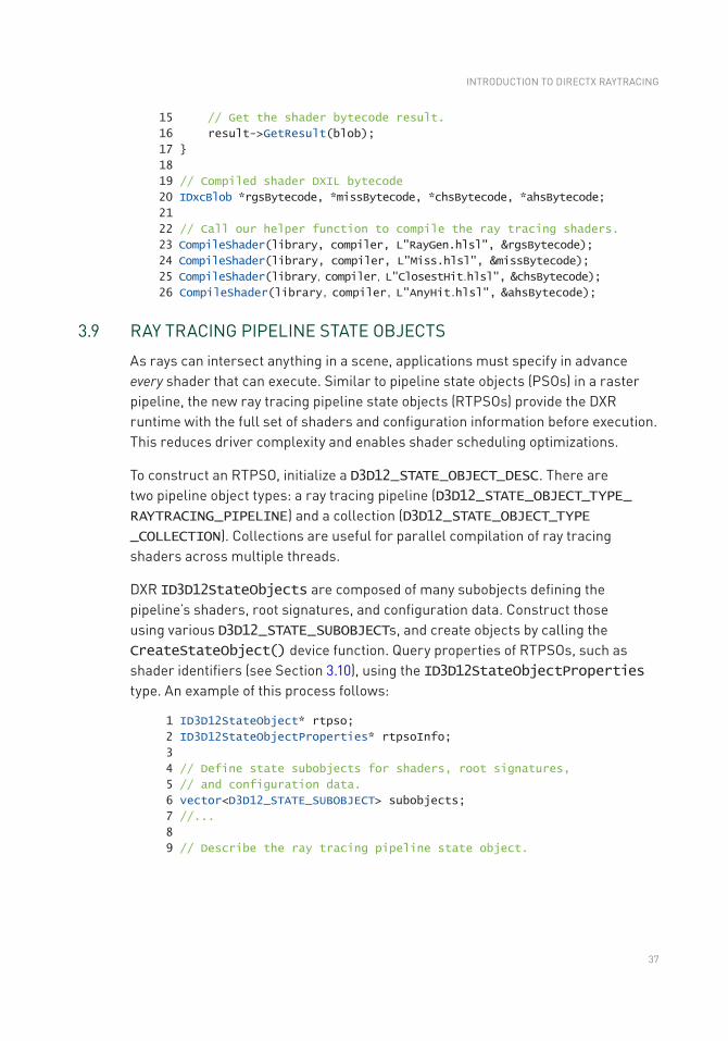
37
15 // Get the shader bytecode result.
16 result->GetResult(blob);
17
18
19 // Compiled shader DXIL bytecode
20 IDxcBlob *rgsBytecode, *missBytecode, *chsBytecode, *ahsBytecode;
21
22 // Call our helper function to compile the ray tracing shaders.
23 CompileShader(library, compiler, L"RayGen.hlsl", &rgsBytecode);
24 CompileShader(library, compiler, L"Miss.hlsl", &missBytecode);
25 CompileShader(library, compiler, L"ClosestHit.hlsl", &chsBytecode);
26 CompileShader(library, compiler, L"AnyHit.hlsl", &ahsBytecode);
3.9 RAY TRACING PIPELINE STATE OBJECTS
As rays can intersect anything in a scene, applications must specify in advance every shader that can execute. Similar to pipeline state objects (PSOs) in a raster pipeline, the new ray tracing pipeline state objects (RTPSOs) provide the DXR runtime with the full set of shaders and configuration information before execution. This reduces driver complexity and enables shader scheduling optimizations.
To construct an RTPSO, initialize a D3D12_STATE_OBJECT_DESC. There are two pipeline object types: a ray tracing pipeline (D3D12_STATE_OBJECT_TYPE_RAYTRACING_PIPELINE) and a collection (D3D12_STATE_OBJECT_TYPE _COLLECTION). Collections are useful for parallel compilation of ray tracing shaders across multiple threads.
DXR ID3D12StateObjects are composed of many subobjects defining the pipeline’s shaders, root signatures, and configuration data. Construct those using various D3D12_STATE_SUBOBJECTs, and create objects by calling the CreateStateObject() device function. Query properties of RTPSOs, such as shader identifiers (see Section 3.10), using the ID3D12StateObjectProperties type. An example of this process follows:
1 ID3D12StateObject* rtpso;
2 ID3D12StateObjectProperties* rtpsoInfo;
3
4 // Define state subobjects for shaders, root signatures,
5 // and configuration data.
6 vector<D3D12_STATE_SUBOBJECT> subobjects;
7 //...
8
9 // Describe the ray tracing pipeline state object.
INTRODUCTION TO DIRECTX RAYTRACING
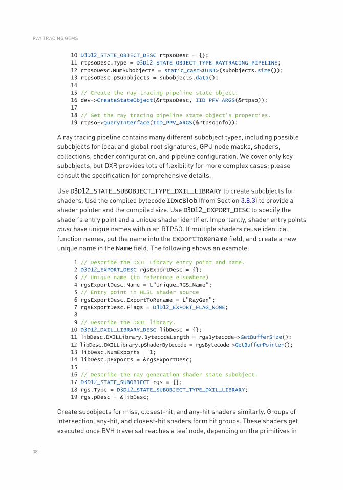
38
10 D3D12_STATE_OBJECT_DESC rtpsoDesc = ;
11 rtpsoDesc.Type = D3D12_STATE_OBJECT_TYPE_RAYTRACING_PIPELINE;
12 rtpsoDesc.NumSubobjects = static_cast<UINT>(subobjects.size());
13 rtpsoDesc.pSubobjects = subobjects.data();
14
15 // Create the ray tracing pipeline state object.
16 dev->CreateStateObject(&rtpsoDesc, IID_PPV_ARGS(&rtpso));
17
18 // Get the ray tracing pipeline state object's properties.
19 rtpso->QueryInterface(IID_PPV_ARGS(&rtpsoInfo));
A ray tracing pipeline contains many different subobject types, including possible subobjects for local and global root signatures, GPU node masks, shaders, collections, shader configuration, and pipeline configuration. We cover only key subobjects, but DXR provides lots of flexibility for more complex cases; please consult the specification for comprehensive details.
Use D3D12_STATE_SUBOBJECT_TYPE_DXIL_LIBRARY to create subobjects for shaders. Use the compiled bytecode IDxcBlob (from Section 3.8.3) to provide a shader pointer and the compiled size. Use D3D12_EXPORT_DESC to specify the shader’s entry point and a unique shader identifier. Importantly, shader entry points must have unique names within an RTPSO. If multiple shaders reuse identical function names, put the name into the ExportToRename field, and create a new unique name in the Name field. The following shows an example:
1 // Describe the DXIL Library entry point and name.
2 D3D12_EXPORT_DESC rgsExportDesc = ;
3 // Unique name (to reference elsewhere)
4 rgsExportDesc.Name = L"Unique_RGS_Name";
5 // Entry point in HLSL shader source
6 rgsExportDesc.ExportToRename = L"RayGen";
7 rgsExportDesc.Flags = D3D12_EXPORT_FLAG_NONE;
8
9 // Describe the DXIL library.
10 D3D12_DXIL_LIBRARY_DESC libDesc = ;
11 libDesc.DXILLibrary.BytecodeLength = rgsBytecode->GetBufferSize();
12 libDesc.DXILLibrary.pShaderBytecode = rgsBytecode->GetBufferPointer();
13 libDesc.NumExports = 1;
14 libDesc.pExports = &rgsExportDesc;
15
16 // Describe the ray generation shader state subobject.
17 D3D12_STATE_SUBOBJECT rgs = ;
18 rgs.Type = D3D12_STATE_SUBOBJECT_TYPE_DXIL_LIBRARY;
19 rgs.pDesc = &libDesc;
Create subobjects for miss, closest-hit, and any-hit shaders similarly. Groups of intersection, any-hit, and closest-hit shaders form hit groups. These shaders get executed once BVH traversal reaches a leaf node, depending on the primitives in
RAY TRACING GEMS
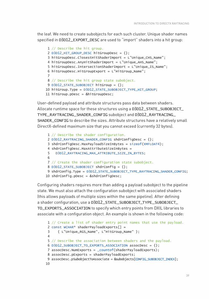
39
the leaf. We need to create subobjects for each such cluster. Unique shader names specified in D3D12_EXPORT_DESC are used to “import” shaders into a hit group:
1 // Describe the hit group.
2 D3D12_HIT_GROUP_DESC hitGroupDesc = ;
3 hitGroupDesc.ClosestHitShaderImport = L"Unique_CHS_Name";
4 hitGroupDesc.AnyHitShaderImport = L"Unique_AHS_Name";
5 hitGroupDesc.IntersectionShaderImport = L"Unique_IS_Name";
6 hitGroupDesc.HitGroupExport = L"HitGroup_Name";
7
8 // Describe the hit group state subobject.
9 D3D12_STATE_SUBOBJECT hitGroup = ;
10 hitGroup.Type = D3D12_STATE_SUBOBJECT_TYPE_HIT_GROUP;
11 hitGroup.pDesc = &hitGroupDesc;
User-defined payload and attribute structures pass data between shaders. Allocate runtime space for these structures using a D3D12_STATE_SUBOBJECT_TYPE_RAYTRACING_SHADER_CONFIG subobject and D3D12_RAYTRACING_SHADER_CONFIG to describe the sizes. Attribute structures have a relatively small DirectX-defined maximum size that you cannot exceed (currently 32 bytes).
1 // Describe the shader configuration.
2 D3D12_RAYTRACING_SHADER_CONFIG shdrConfigDesc = ;
3 shdrConfigDesc.MaxPayloadSizeInBytes = sizeof(XMFLOAT4);
4 shdrConfigDesc.MaxAttributeSizeInBytes =
5 D3D12_RAYTRACING_MAX_ATTRIBUTE_SIZE_IN_BYTES;
6
7 // Create the shader configuration state subobject.
8 D3D12_STATE_SUBOBJECT shdrConfig = ;
9 shdrConfig.Type = D3D12_STATE_SUBOBJECT_TYPE_RAYTRACING_SHADER_CONFIG;
10 shdrConfig.pDesc = &shdrConfigDesc;
Configuring shaders requires more than adding a payload subobject to the pipeline state. We must also attach the configuration subobject with associated shaders (this allows payloads of multiple sizes within the same pipeline). After defining a shader configuration, use a D3D12_STATE_SUBOBJECT_TYPE_SUBOBJECT_TO_EXPORTS_ASSOCIATION to specify which entry points from DXIL libraries to associate with a configuration object. An example is shown in the following code:
1 // Create a list of shader entry point names that use the payload.
2 const WCHAR* shaderPayloadExports[] =
3 L"Unique_RGS_Name", L"HitGroup_Name" ;
4
5 // Describe the association between shaders and the payload.
6 D3D12_SUBOBJECT_TO_EXPORTS_ASSOCIATION assocDesc = ;
7 assocDesc.NumExports = _countof(shaderPayloadExports);
8 assocDesc.pExports = shaderPayloadExports;
9 assocDesc.pSubobjectToAssociate = &subobjects[CONFIG_SUBOBJECT_INDEX];
10
INTRODUCTION TO DIRECTX RAYTRACING
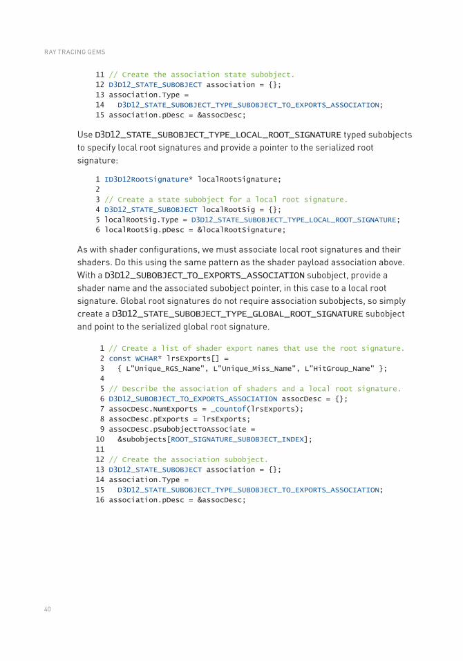
40
11 // Create the association state subobject.
12 D3D12_STATE_SUBOBJECT association = ;
13 association.Type =
14 D3D12_STATE_SUBOBJECT_TYPE_SUBOBJECT_TO_EXPORTS_ASSOCIATION;
15 association.pDesc = &assocDesc;
Use D3D12_STATE_SUBOBJECT_TYPE_LOCAL_ROOT_SIGNATURE typed subobjects to specify local root signatures and provide a pointer to the serialized root signature:
1 ID3D12RootSignature* localRootSignature;
2
3 // Create a state subobject for a local root signature.
4 D3D12_STATE_SUBOBJECT localRootSig = ;
5 localRootSig.Type = D3D12_STATE_SUBOBJECT_TYPE_LOCAL_ROOT_SIGNATURE;
6 localRootSig.pDesc = &localRootSignature;
As with shader configurations, we must associate local root signatures and their shaders. Do this using the same pattern as the shader payload association above. With a D3D12_SUBOBJECT_TO_EXPORTS_ASSOCIATION subobject, provide a shader name and the associated subobject pointer, in this case to a local root signature. Global root signatures do not require association subobjects, so simply create a D3D12_STATE_SUBOBJECT_TYPE_GLOBAL_ROOT_SIGNATURE subobject and point to the serialized global root signature.
1 // Create a list of shader export names that use the root signature.
2 const WCHAR* lrsExports[] =
3 L"Unique_RGS_Name", L"Unique_Miss_Name", L"HitGroup_Name" ;
4
5 // Describe the association of shaders and a local root signature.
6 D3D12_SUBOBJECT_TO_EXPORTS_ASSOCIATION assocDesc = ;
7 assocDesc.NumExports = _countof(lrsExports);
8 assocDesc.pExports = lrsExports;
9 assocDesc.pSubobjectToAssociate =
10 &subobjects[ROOT_SIGNATURE_SUBOBJECT_INDEX];
11
12 // Create the association subobject.
13 D3D12_STATE_SUBOBJECT association = ;
14 association.Type =
15 D3D12_STATE_SUBOBJECT_TYPE_SUBOBJECT_TO_EXPORTS_ASSOCIATION;
16 association.pDesc = &assocDesc;
RAY TRACING GEMS
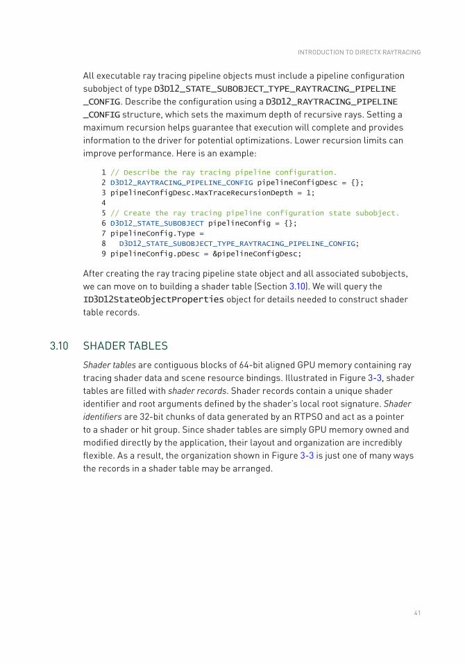
41
All executable ray tracing pipeline objects must include a pipeline configuration subobject of type D3D12_STATE_SUBOBJECT_TYPE_RAYTRACING_PIPELINE _CONFIG. Describe the configuration using a D3D12_RAYTRACING_PIPELINE _CONFIG structure, which sets the maximum depth of recursive rays. Setting a maximum recursion helps guarantee that execution will complete and provides information to the driver for potential optimizations. Lower recursion limits can improve performance. Here is an example:
1 // Describe the ray tracing pipeline configuration.
2 D3D12_RAYTRACING_PIPELINE_CONFIG pipelineConfigDesc = ;
3 pipelineConfigDesc.MaxTraceRecursionDepth = 1;
4
5 // Create the ray tracing pipeline configuration state subobject.
6 D3D12_STATE_SUBOBJECT pipelineConfig = ;
7 pipelineConfig.Type =
8 D3D12_STATE_SUBOBJECT_TYPE_RAYTRACING_PIPELINE_CONFIG;
9 pipelineConfig.pDesc = &pipelineConfigDesc;
After creating the ray tracing pipeline state object and all associated subobjects, we can move on to building a shader table (Section 3.10). We will query the ID3D12StateObjectProperties object for details needed to construct shader table records.
3.10 SHADER TABLES
Shader tables are contiguous blocks of 64-bit aligned GPU memory containing ray tracing shader data and scene resource bindings. Illustrated in Figure 3-3, shader tables are filled with shader records. Shader records contain a unique shader identifier and root arguments defined by the shader’s local root signature. Shader identifiers are 32-bit chunks of data generated by an RTPSO and act as a pointer to a shader or hit group. Since shader tables are simply GPU memory owned and modified directly by the application, their layout and organization are incredibly flexible. As a result, the organization shown in Figure 3-3 is just one of many ways the records in a shader table may be arranged.
INTRODUCTION TO DIRECTX RAYTRACING
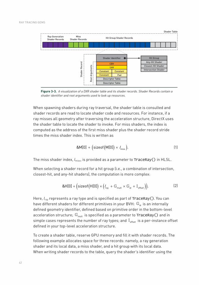
42
When spawning shaders during ray traversal, the shader table is consulted and shader records are read to locate shader code and resources. For instance, if a ray misses all geometry after traversing the acceleration structure, DirectX uses the shader table to locate the shader to invoke. For miss shaders, the index is computed as the address of the first miss shader plus the shader record stride times the miss shader index. This is written as
( )( )Imiss&M[0] sizeof M[0] .+ ´
(1)
The miss shader index, Imiss, is provided as a parameter to TraceRay() in HLSL.
When selecting a shader record for a hit group (i.e., a combination of intersection, closest-hit, and any-hit shaders), the computation is more complex:
( ) ( )( )ray mult id offset&H[0] sizeof H[0] .I+ ´ + ´ +
(2)
Here, Iray represents a ray type and is specified as part of TraceRay(). You can have different shaders for different primitives in your BVH: id is an internally defined geometry identifier, defined based on primitive order in the bottom-level acceleration structure; mult is specified as a parameter to TraceRay() and in simple cases represents the number of ray types; and offset is a per-instance offset defined in your top-level acceleration structure.
To create a shader table, reserve GPU memory and fill it with shader records. The following example allocates space for three records: namely, a ray generation shader and its local data, a miss shader, and a hit group with its local data. When writing shader records to the table, query the shader’s identifier using the
Figure 3-3. A visualization of a DXR shader table and its shader records. Shader Records contain a shader identifier and root arguments used to look up resources.
RAY TRACING GEMS
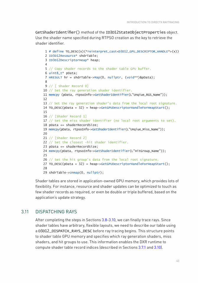
43
GetShaderIdentifier() method of the ID3D12StateObjectProperties object. Use the shader name specified during RTPSO creation as the key to retrieve the shader identifier.
1 # define TO_DESC(x)(*reinterpret_cast<D3D12_GPU_DESCRIPTOR_HANDLE*>(x))
2 ID3D12Resource* shdrTable;
3 ID3D12DescriptorHeap* heap;
4
5 // Copy shader records to the shader table GPU buffer.
6 uint8_t* pData;
7 HRESULT hr = shdrTable->Map(0, nullptr, (void**)&pData);
8
9 // [ Shader Record 0]
10 // Set the ray generation shader identifier.
11 memcpy (pData, rtpsoInfo->GetShaderIdentifier(L"Unqiue_RGS_Name"));
12
13 // Set the ray generation shader's data from the local root signature.
14 TO_DESC(pData + 32) = heap->GetGPUDescriptorHandleForHeapStart();
15
16 // [Shader Record 1]
17 // Set the miss shader identifier (no local root arguments to set).
18 pData += shaderRecordSize;
19 memcpy(pData, rtpsoInfo->GetShaderIdentifier(L"Unqiue_Miss_Name"));
20
21 // [Shader Record 2]
22 // Set the closest -hit shader identifier.
23 pData += shaderRecordSize;
24 memcpy(pData, rtpsoInfo->GetShaderIdentifier(L"HitGroup_Name"));
25
26 // Set the hit group's data from the local root signature.
27 TO_DESC(pData + 32) = heap->GetGPUDescriptorHandleForHeapStart();
28
29 shdrTable->Unmap(0, nullptr);
Shader tables are stored in application-owned GPU memory, which provides lots of flexibility. For instance, resource and shader updates can be optimized to touch as few shader records as required, or even be double or triple buffered, based on the application’s update strategy.
3.11 DISPATCHING RAYS
After completing the steps in Sections 3.8-3.10, we can finally trace rays. Since shader tables have arbitrary, flexible layouts, we need to describe our table using a D3D12_DISPATCH_RAYS_DESC before ray tracing begins. This structure points to shader table GPU memory and specifies which ray generation shaders, miss shaders, and hit groups to use. This information enables the DXR runtime to compute shader table record indices (described in Sections 3.7.1 and 3.10).
INTRODUCTION TO DIRECTX RAYTRACING
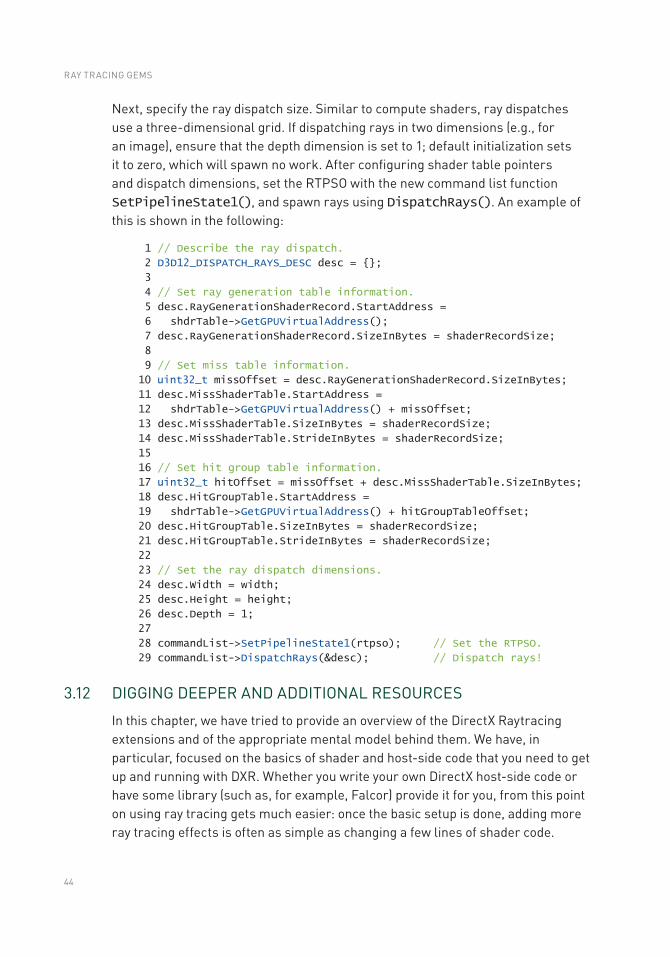
44
Next, specify the ray dispatch size. Similar to compute shaders, ray dispatches use a three-dimensional grid. If dispatching rays in two dimensions (e.g., for an image), ensure that the depth dimension is set to 1; default initialization sets it to zero, which will spawn no work. After configuring shader table pointers and dispatch dimensions, set the RTPSO with the new command list function SetPipelineState1(), and spawn rays using DispatchRays(). An example of this is shown in the following:
1 // Describe the ray dispatch.
2 D3D12_DISPATCH_RAYS_DESC desc = ;
3
4 // Set ray generation table information.
5 desc.RayGenerationShaderRecord.StartAddress =
6 shdrTable->GetGPUVirtualAddress();
7 desc.RayGenerationShaderRecord.SizeInBytes = shaderRecordSize;
8
9 // Set miss table information.
10 uint32_t missOffset = desc.RayGenerationShaderRecord.SizeInBytes;
11 desc.MissShaderTable.StartAddress =
12 shdrTable->GetGPUVirtualAddress() + missOffset;
13 desc.MissShaderTable.SizeInBytes = shaderRecordSize;
14 desc.MissShaderTable.StrideInBytes = shaderRecordSize;
15
16 // Set hit group table information.
17 uint32_t hitOffset = missOffset + desc.MissShaderTable.SizeInBytes;
18 desc.HitGroupTable.StartAddress =
19 shdrTable->GetGPUVirtualAddress() + hitGroupTableOffset;
20 desc.HitGroupTable.SizeInBytes = shaderRecordSize;
21 desc.HitGroupTable.StrideInBytes = shaderRecordSize;
22
23 // Set the ray dispatch dimensions.
24 desc.Width = width;
25 desc.Height = height;
26 desc.Depth = 1;
27
28 commandList->SetPipelineState1(rtpso); // Set the RTPSO.
29 commandList->DispatchRays(&desc); // Dispatch rays!
3.12 DIGGING DEEPER AND ADDITIONAL RESOURCES
In this chapter, we have tried to provide an overview of the DirectX Raytracing extensions and of the appropriate mental model behind them. We have, in particular, focused on the basics of shader and host-side code that you need to get up and running with DXR. Whether you write your own DirectX host-side code or have some library (such as, for example, Falcor) provide it for you, from this point on using ray tracing gets much easier: once the basic setup is done, adding more ray tracing effects is often as simple as changing a few lines of shader code.
RAY TRACING GEMS
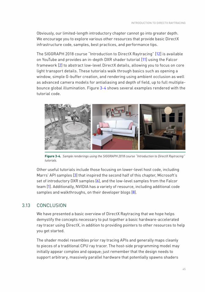
45
Obviously, our limited-length introductory chapter cannot go into greater depth. We encourage you to explore various other resources that provide basic DirectX infrastructure code, samples, best practices, and performance tips.
The SIGGRAPH 2018 course “Introduction to DirectX Raytracing” [12] is available on YouTube and provides an in-depth DXR shader tutorial [11] using the Falcor framework [2] to abstract low-level DirectX details, allowing you to focus on core light transport details. These tutorials walk through basics such as opening a window, simple G-buffer creation, and rendering using ambient occlusion as well as advanced camera models for antialiasing and depth of field, up to full multiple-bounce global illumination. Figure 3-4 shows several examples rendered with the tutorial code.
Figure 3-4. Sample renderings using the SIGGRAPH 2018 course “Introduction to DirectX Raytracing” tutorials.
Other useful tutorials include those focusing on lower-level host code, including Marrs’ API samples [3] that inspired the second half of this chapter, Microsoft’s set of introductory DXR samples [6], and the low-level samples from the Falcor team [1]. Additionally, NVIDIA has a variety of resource, including additional code samples and walkthroughs, on their developer blogs [8].
3.13 CONCLUSION
We have presented a basic overview of DirectX Raytracing that we hope helps demystify the concepts necessary to put together a basic hardware-accelerated ray tracer using DirectX, in addition to providing pointers to other resources to help you get started.
The shader model resembles prior ray tracing APIs and generally maps cleanly to pieces of a traditional CPU ray tracer. The host-side programming model may initially appear complex and opaque; just remember that the design needs to support arbitrary, massively parallel hardware that potentially spawns shaders
INTRODUCTION TO DIRECTX RAYTRACING
46
without the benefit of a continuous execution history along each ray. New DXR pipeline state objects and shader tables help to specify data and shaders so such GPUs can spawn work arbitrarily as rays traverse the scene.
Given the complexities of DirectX 12 and the flexibility of ray tracing, we were unable to fully cover the API. Our goal was to provide enough information to get started. As you target more complex renderings, you will need to refer to the DXR specification or other documentation for further guidance. In particular, more complex shader compilation, default pipeline subobject settings, system limits, error handling, and tips for optimal performance all will require other references.
Our advice for getting starting: begin simply. Key problems revolve around correctly setting up the ray tracing pipeline state objects and the shader table, and these are much easier to debug with fewer, simple shaders. For example, basic ray traced shadowing or ambient occlusion using a rasterized G-buffer for primary visibility are good starting points.
With DirectX Raytracing and modern GPUs, shooting rays is faster than ever. However, ray tracing is not free. For at least the near future, you can assume at most a few rays per pixel. This means hybrid ray-raster algorithms, antialiasing, denoising, and reconstruction will all be vital to achieve high-quality renderings quickly. Other work in this book provides ideas on some of these topics, but many problems remain unsolved.
REFERENCES
[1] Benty, N. DirectX Raytracing Tutorials. https://github.com/NVIDIAGameWorks/DxrTutorials, 2018. Accessed October 25, 2018.
[2] Benty, N., Yao, K.-H., Foley, T., Kaplanyan, A. S., Lavelle, C., Wyman, C., and Vijay, A. The Falcor Rendering Framework. https://github.com/NVIDIAGameWorks/Falcor, July 2017.
[3] Marrs, A. Introduction to DirectX Raytracing. https://github.com/acmarrs/IntroToDXR, 2018. Accessed October 25, 2018.
[4] Marschner, S., and Shirley, P. Fundamentals of Computer Graphics, fourth ed. CRC Press, 2015.
[5] Microsoft. Programming Guide and Reference for HLSL. https://docs.microsoft.com/en-us/windows/desktop/direct3dhlsl/dx-graphics-hlsl. Accessed October 25, 2018.
[6] Microsoft. D3D12 Raytracing Samples. https://github.com/Microsoft/DirectX- Graphics- Samples/tree/master/Samples/Desktop/D3D12Raytracing, 2018. Accessed October 25, 2018.
[7] Microsoft. DirectX Shader Compiler. https://github.com/Microsoft/DirectXShaderCompiler, 2018. Accessed October 30, 2018.
RAY TRACING GEMS

47
[8] NVIDIA. DirectX Raytracing Developer Blogs. https://devblogs.nvidia.com/tag/dxr/, 2018. Accessed October 25, 2018.
[9] Shirley, P. Ray Tracing in One Weekend. Amazon Digital Services LLC, 2016. https://github.com/petershirley/raytracinginoneweekend.
[10] Suffern, K. Ray Tracing from the Ground Up. A K Peters, 2007.
[11] Wyman, C. A Gentle Introduction To DirectX Raytracing. http://cwyman.org/code/dxrTutors/dxr_tutors.md.html, 2018.
[12] Wyman, C., Hargreaves, S., Shirley, P., and Barré-Brisebois, C. Introduction to DirectX Raytracing. SIGGRAPH Courses, 2018. http://intro-to-dxr.cwyman.org, https://www.youtube.com/watch?v=Q1cuuepVNoY.
Open Access This chapter is licensed under the terms of the Creative Commons Attribution-NonCommercial-NoDerivatives 4.0 International License (http://creativecommons.org/licenses/by-nc-nd/4.0/), which permits any noncommercial use, sharing, distribution and
reproduction in any medium or format, as long as you give appropriate credit to the original author(s) and the source, provide a link to the Creative Commons license and indicate if you modified the licensed material. You do not have permission under this license to share adapted material derived from this chapter or parts of it.
The images or other third party material in this chapter are included in the chapter's Creative Commons license, unless indicated otherwise in a credit line to the material. If material is not included in the chapter's Creative Commons license and your intended use is not permitted by statutory regulation or exceeds the permitted use, you will need to obtain permission directly from the copyright holder.
INTRODUCTION TO DIRECTX RAYTRACING
49© NVIDIA 2019 E. Haines, T. Akenine-Möller (eds.), Ray Tracing Gems, https://doi.org/10.1007/978-1-4842-4427-2_4
CHAPTER 4
A Planetarium Dome Master CameraJohn E. Stone Beckman Institute for Advanced Science and Technology, University of Illinois at Urbana-Champaign
ABSTRACT
This chapter presents a camera implementation for high-quality interactive ray tracing of planetarium dome master images using an azimuthal equidistant projection. Ray tracing is aptly suited for implementing a wide variety of special panoramic and stereoscopic projections without sacrificing image quality. This camera implementation supports antialiasing, depth of field focal blur, and circular stereoscopic projections, all effects that are difficult to produce with high quality using conventional rasterization and image warping.
4.1 INTRODUCTION
Planetarium dome master images encode a 180° hemispherical field of view within a black square, with an inscribed circular image containing the entire field of view for projection onto a planetarium dome. Dome master images are produced using a so-called azimuthal equidistant projection and closely match the output of a real-world 180° equidistant fisheye lens, but without a real lens’ imperfections and optical aberrations. There are many ways of creating dome master projections using rasterization and image warping techniques, but direct ray tracing has particular advantages over other alternatives: uniform sample density in the final dome master image (no samples are wasted in oversampled areas as when warping cubic projections or many planar perspective projections [3]), support for stereoscopic rendering, and support for depth of field on an intrinsically curved focal surface. By integrating interactive progressive ray tracing of dome master images within scientific visualization software, a much broader range of scientific visualization material can be made available in public fulldome projection venues [1, 5, 7].
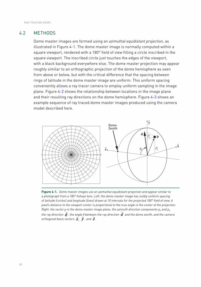
50
4.2 METHODS
Dome master images are formed using an azimuthal equidistant projection, as illustrated in Figure 4-1. The dome master image is normally computed within a square viewport, rendered with a 180° field of view filling a circle inscribed in the square viewport. The inscribed circle just touches the edges of the viewport, with a black background everywhere else. The dome master projection may appear roughly similar to an orthographic projection of the dome hemisphere as seen from above or below, but with the critical difference that the spacing between rings of latitude in the dome master image are uniform. This uniform spacing conveniently allows a ray tracer camera to employ uniform sampling in the image plane. Figure 4-2 shows the relationship between locations in the image plane and their resulting ray directions on the dome hemisphere. Figure 4-3 shows an example sequence of ray traced dome master images produced using the camera model described here.
Figure 4-1. Dome master images use an azimuthal equidistant projection and appear similar to a photograph from a 180° fisheye lens. Left: the dome master image has visibly uniform spacing of latitude (circles) and longitude (lines) drawn at 10 intervals for the projected 180° field of view. A pixel’s distance to the viewport center is proportional to the true angle in the center of the projection. Right: the vector p in the dome master image plane, the azimuth direction components px and py,
the ray direction d , the angle θ between the ray direction d and the dome zenith, and the camera orthogonal basis vectors ,x y , and z .
RAY TRACING GEMS
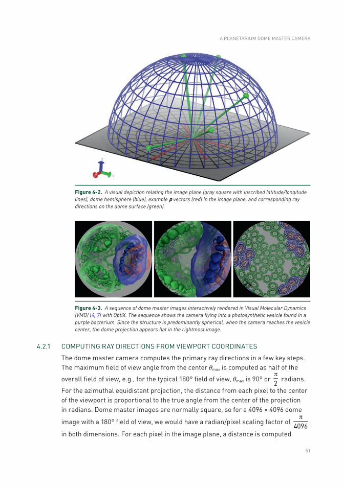
51
Figure 4-2. A visual depiction relating the image plane (gray square with inscribed latitude/longitude lines), dome hemisphere (blue), example p vectors (red) in the image plane, and corresponding ray directions on the dome surface (green).
Figure 4-3. A sequence of dome master images interactively rendered in Visual Molecular Dynamics (VMD) [4, 7] with OptiX. The sequence shows the camera flying into a photosynthetic vesicle found in a purple bacterium. Since the structure is predominantly spherical, when the camera reaches the vesicle center, the dome projection appears flat in the rightmost image.
4.2.1 COMPUTING RAY DIRECTIONS FROM VIEWPORT COORDINATES
The dome master camera computes the primary ray directions in a few key steps. The maximum field of view angle from the center θmax is computed as half of the
overall field of view, e.g., for the typical 180° field of view, θmax is 90° or 2p
radians.
For the azimuthal equidistant projection, the distance from each pixel to the center of the viewport is proportional to the true angle from the center of the projection in radians. Dome master images are normally square, so for a 4096 × 4096 dome
image with a 180° field of view, we would have a radian/pixel scaling factor of 4096p
in both dimensions. For each pixel in the image plane, a distance is computed
A PlANETARIUM DOME MASTER CAMERA
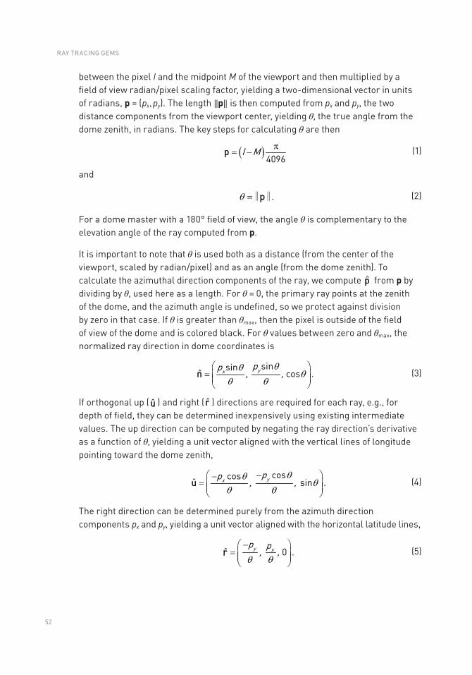
52
between the pixel I and the midpoint M of the viewport and then multiplied by a field of view radian/pixel scaling factor, yielding a two-dimensional vector in units of radians, p = (px, py). The length ‖p‖ is then computed from px and py, the two distance components from the viewport center, yielding θ, the true angle from the dome zenith, in radians. The key steps for calculating θ are then
( )I M
4096p
= -p
(1)
and
.q = p‖‖ (2)
For a dome master with a 180° field of view, the angle θ is complementary to the elevation angle of the ray computed from p.
It is important to note that θ is used both as a distance (from the center of the viewport, scaled by radian/pixel) and as an angle (from the dome zenith). To calculate the azimuthal direction components of the ray, we compute p from p by dividing by θ, used here as a length. For θ = 0, the primary ray points at the zenith of the dome, and the azimuth angle is undefined, so we protect against division by zero in that case. If θ is greater than θmax, then the pixel is outside of the field of view of the dome and is colored black. For θ values between zero and θmax, the normalized ray direction in dome coordinates is
yxpp
, , sinsin
cosˆ .qq
qq q
æ ö= ç ÷ç ÷è ø
n (3)
If orthogonal up ( u ) and right ( r ) directions are required for each ray, e.g., for depth of field, they can be determined inexpensively using existing intermediate values. The up direction can be computed by negating the ray direction’s derivative as a function of θ, yielding a unit vector aligned with the vertical lines of longitude pointing toward the dome zenith,
yxpp
, , coscos
sin .ˆqq
qq q
æ - ö-= ç ÷ç ÷è ø
u (4)
The right direction can be determined purely from the azimuth direction components px and py, yielding a unit vector aligned with the horizontal latitude lines,
y xp p
, , .ˆ 0q q
æ - ö= ç ÷ç ÷è ø
r (5)
RAY TRACING GEMS
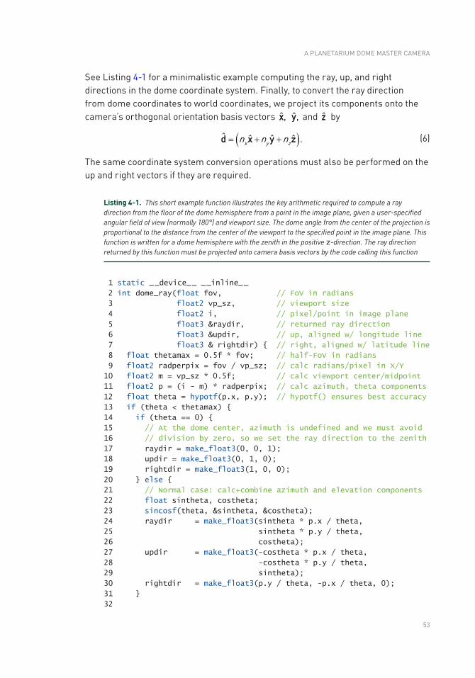
53
See listing 4-1 for a minimalistic example computing the ray, up, and right directions in the dome coordinate system. Finally, to convert the ray direction from dome coordinates to world coordinates, we project its components onto the camera’s orthogonal orientation basis vectors ˆ,x ˆ,y and z by
( )x y zn n nˆ ˆ ˆ ˆ .= + +d x y z (6)
The same coordinate system conversion operations must also be performed on the up and right vectors if they are required.
Listing 4-1. This short example function illustrates the key arithmetic required to compute a ray direction from the floor of the dome hemisphere from a point in the image plane, given a user-specified angular field of view (normally 180°) and viewport size. The dome angle from the center of the projection is proportional to the distance from the center of the viewport to the specified point in the image plane. This function is written for a dome hemisphere with the zenith in the positive z-direction. The ray direction returned by this function must be projected onto camera basis vectors by the code calling this function
1 static _ _device_ _ _ _inline_ _
2 int dome_ray(float fov, // FoV in radians
3 float2 vp_sz, // viewport size
4 float2 i, // pixel/point in image plane
5 float3 &raydir, // returned ray direction
6 float3 &updir, // up, aligned w/ longitude line
7 float3 & rightdir) // right, aligned w/ latitude line
8 float thetamax = 0.5f * fov; // half-FoV in radians
9 float2 radperpix = fov / vp_sz; // calc radians/pixel in X/Y
10 float2 m = vp_sz * 0.5f; // calc viewport center/midpoint
11 float2 p = (i - m) * radperpix; // calc azimuth, theta components
12 float theta = hypotf(p.x, p.y); // hypotf() ensures best accuracy
13 if (theta < thetamax)
14 if (theta == 0)
15 // At the dome center, azimuth is undefined and we must avoid
16 // division by zero, so we set the ray direction to the zenith
17 raydir = make_float3(0, 0, 1);
18 updir = make_float3(0, 1, 0);
19 rightdir = make_float3(1, 0, 0);
20 else
21 // Normal case: calc+combine azimuth and elevation components
22 float sintheta, costheta;
23 sincosf(theta, &sintheta, &costheta);
24 raydir = make_float3(sintheta * p.x / theta,
25 sintheta * p.y / theta,
26 costheta);
27 updir = make_float3(-costheta * p.x / theta,
28 -costheta * p.y / theta,
29 sintheta);
30 rightdir = make_float3(p.y / theta, -p.x / theta, 0);
31
32
A PlANETARIUM DOME MASTER CAMERA
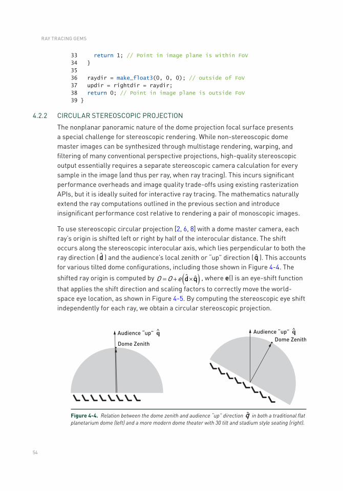
54
33 return 1; // Point in image plane is within FoV
34
35
36 raydir = make_float3(0, 0, 0); // outside of FoV
37 updir = rightdir = raydir;
38 return 0; // Point in image plane is outside FoV
39
4.2.2 CIRCUlAR STEREOSCOPIC PROJECTION
The nonplanar panoramic nature of the dome projection focal surface presents a special challenge for stereoscopic rendering. While non-stereoscopic dome master images can be synthesized through multistage rendering, warping, and filtering of many conventional perspective projections, high-quality stereoscopic output essentially requires a separate stereoscopic camera calculation for every sample in the image (and thus per ray, when ray tracing). This incurs significant performance overheads and image quality trade-offs using existing rasterization APIs, but it is ideally suited for interactive ray tracing. The mathematics naturally extend the ray computations outlined in the previous section and introduce insignificant performance cost relative to rendering a pair of monoscopic images.
To use stereoscopic circular projection [2, 6, 8] with a dome master camera, each ray’s origin is shifted left or right by half of the interocular distance. The shift occurs along the stereoscopic interocular axis, which lies perpendicular to both the ray direction ( d ) and the audience’s local zenith or “up” direction ( q ). This accounts for various tilted dome configurations, including those shown in Figure 4-4. The
shifted ray origin is computed by ( )O O e ˆ ˆ= + ´d q , where e() is an eye-shift function
that applies the shift direction and scaling factors to correctly move the world-space eye location, as shown in Figure 4-5. By computing the stereoscopic eye shift independently for each ray, we obtain a circular stereoscopic projection.
Figure 4-4. Relation between the dome zenith and audience “up” direction q in both a traditional flat planetarium dome (left) and a more modern dome theater with 30 tilt and stadium style seating (right).
RAY TRACING GEMS
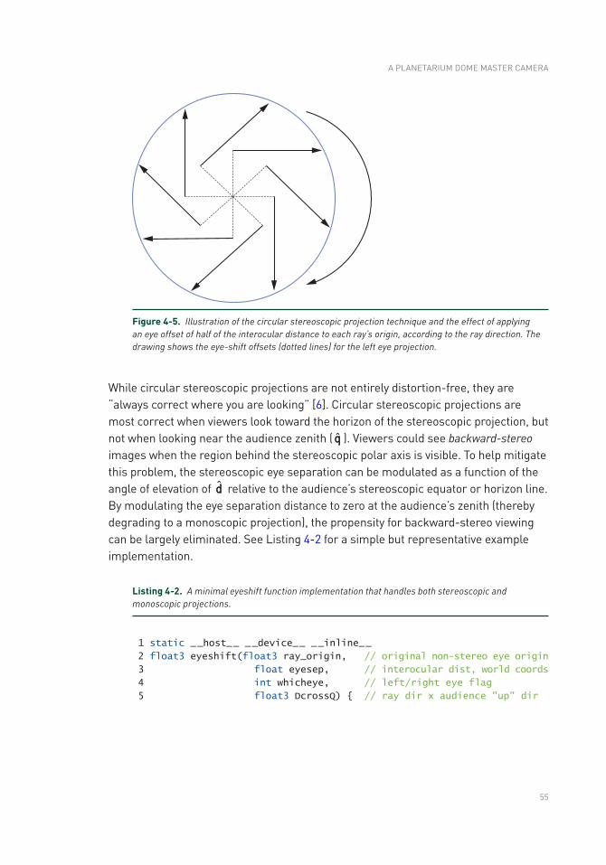
55
While circular stereoscopic projections are not entirely distortion-free, they are “always correct where you are looking” [6]. Circular stereoscopic projections are most correct when viewers look toward the horizon of the stereoscopic projection, but not when looking near the audience zenith ( q ). Viewers could see backward-stereo images when the region behind the stereoscopic polar axis is visible. To help mitigate this problem, the stereoscopic eye separation can be modulated as a function of the angle of elevation of d relative to the audience’s stereoscopic equator or horizon line. By modulating the eye separation distance to zero at the audience’s zenith (thereby degrading to a monoscopic projection), the propensity for backward-stereo viewing can be largely eliminated. See listing 4-2 for a simple but representative example implementation.
Listing 4-2. A minimal eyeshift function implementation that handles both stereoscopic and monoscopic projections.
1 static _ _host_ _ _ _device_ _ _ _inline_ _
2 float3 eyeshift(float3 ray_origin, // original non-stereo eye origin
3 float eyesep, // interocular dist, world coords
4 int whicheye, // left/right eye flag
5 float3 DcrossQ) // ray dir x audience "up" dir
Figure 4-5. Illustration of the circular stereoscopic projection technique and the effect of applying an eye offset of half of the interocular distance to each ray’s origin, according to the ray direction. The drawing shows the eye-shift offsets (dotted lines) for the left eye projection.
A PlANETARIUM DOME MASTER CAMERA
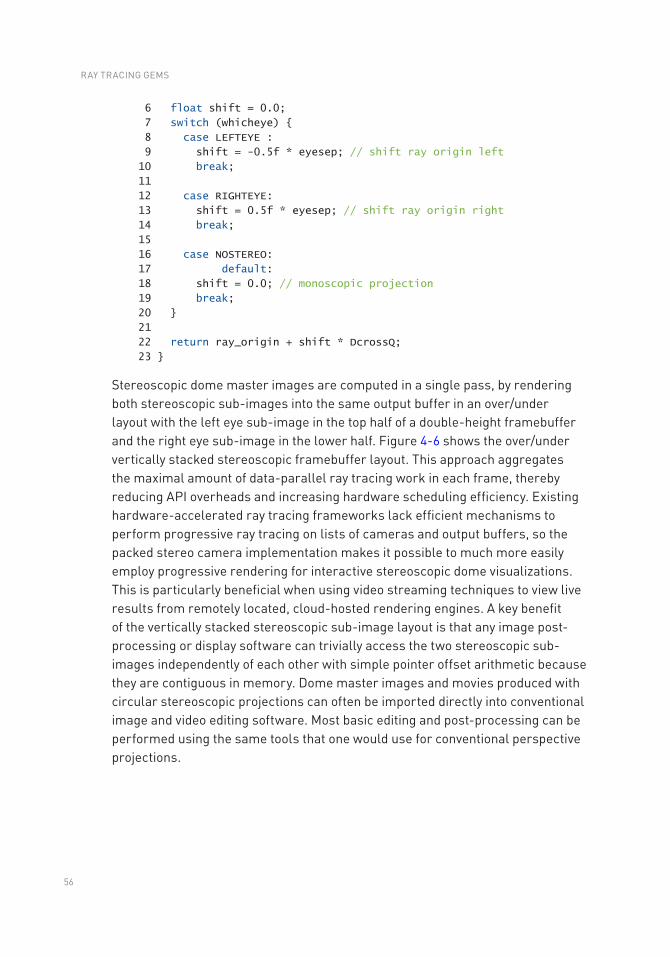
56
6 float shift = 0.0;
7 switch (whicheye)
8 case LEFTEYE :
9 shift = -0.5f * eyesep; // shift ray origin left
10 break;
11
12 case RIGHTEYE:
13 shift = 0.5f * eyesep; // shift ray origin right
14 break;
15
16 case NOSTEREO:
17 default:
18 shift = 0.0; // monoscopic projection
19 break;
20
21
22 return ray_origin + shift * DcrossQ;
23
Stereoscopic dome master images are computed in a single pass, by rendering both stereoscopic sub-images into the same output buffer in an over/under layout with the left eye sub-image in the top half of a double-height framebuffer and the right eye sub- image in the lower half. Figure 4-6 shows the over/under vertically stacked stereoscopic framebuffer layout. This approach aggregates the maximal amount of data-parallel ray tracing work in each frame, thereby reducing API overheads and increasing hardware scheduling efficiency. Existing hardware-accelerated ray tracing frameworks lack efficient mechanisms to perform progressive ray tracing on lists of cameras and output buffers, so the packed stereo camera implementation makes it possible to much more easily employ progressive rendering for interactive stereoscopic dome visualizations. This is particularly beneficial when using video streaming techniques to view live results from remotely located, cloud-hosted rendering engines. A key benefit of the vertically stacked stereoscopic sub-image layout is that any image post-processing or display software can trivially access the two stereoscopic sub-images independently of each other with simple pointer offset arithmetic because they are contiguous in memory. Dome master images and movies produced with circular stereoscopic projections can often be imported directly into conventional image and video editing software. Most basic editing and post-processing can be performed using the same tools that one would use for conventional perspective projections.
RAY TRACING GEMS
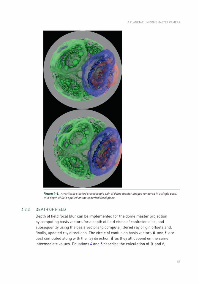
57
4.2.3 DEPTH OF FIElD
Depth of field focal blur can be implemented for the dome master projection by computing basis vectors for a depth of field circle of confusion disk, and subsequently using the basis vectors to compute jittered ray origin offsets and, finally, updated ray directions. The circle of confusion basis vectors u and r are best computed along with the ray direction d as they all depend on the same intermediate values. Equations 4 and 5 describe the calculation of u and ,r
Figure 4-6. A vertically stacked stereoscopic pair of dome master images rendered in a single pass, with depth of field applied on the spherical focal plane.
A PlANETARIUM DOME MASTER CAMERA
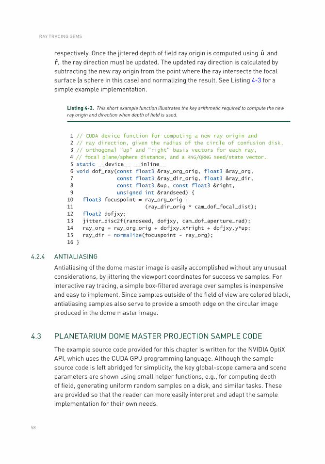
58
respectively. Once the jittered depth of field ray origin is computed using u and ,r the ray direction must be updated. The updated ray direction is calculated by
subtracting the new ray origin from the point where the ray intersects the focal surface (a sphere in this case) and normalizing the result. See listing 4-3 for a simple example implementation.
Listing 4-3. This short example function illustrates the key arithmetic required to compute the new ray origin and direction when depth of field is used.
1 // CUDA device function for computing a new ray origin and
2 // ray direction, given the radius of the circle of confusion disk,
3 // orthogonal "up" and "right" basis vectors for each ray,
4 // focal plane/sphere distance, and a RNG/QRNG seed/state vector.
5 static _ _device_ _ _ _inline_ _
6 void dof_ray(const float3 &ray_org_orig, float3 &ray_org,
7 const float3 &ray_dir_orig, float3 &ray_dir,
8 const float3 &up, const float3 &right,
9 unsigned int &randseed)
10 float3 focuspoint = ray_org_orig +
11 (ray_dir_orig * cam_dof_focal_dist);
12 float2 dofjxy;
13 jitter_disc2f(randseed, dofjxy, cam_dof_aperture_rad);
14 ray_org = ray_org_orig + dofjxy.x*right + dofjxy.y*up;
15 ray_dir = normalize(focuspoint - ray_org);
16
4.2.4 ANTIAlIASING
Antialiasing of the dome master image is easily accomplished without any unusual considerations, by jittering the viewport coordinates for successive samples. For interactive ray tracing, a simple box-filtered average over samples is inexpensive and easy to implement. Since samples outside of the field of view are colored black, antialiasing samples also serve to provide a smooth edge on the circular image produced in the dome master image.
4.3 PlANETARIUM DOME MASTER PROJECTION SAMPlE CODE
The example source code provided for this chapter is written for the NVIDIA OptiX API, which uses the CUDA GPU programming language. Although the sample source code is left abridged for simplicity, the key global-scope camera and scene parameters are shown using small helper functions, e.g., for computing depth of field, generating uniform random samples on a disk, and similar tasks. These are provided so that the reader can more easily interpret and adapt the sample implementation for their own needs.
RAY TRACING GEMS
59
The dome master camera is implemented as a templated camera function, to be instantiated in several primary ray generation “programs” for the OptiX ray tracing framework. The function accepts STEREO_ON and DOF_ON template parameters that either enable or disable generation of a stereoscopic dome master image and depth of field focal blur, respectively. By creating separate instantiations of the camera function, arithmetic operations associated with disabled features are eliminated, which is particularly beneficial for high-resolution interactive ray tracing of complex scenes.
ACKNOWlEDGMENTS
This work was supported in part by the National Institutes of Health, under grant P41-GM104601; the NCSA Advanced Visualization laboratory; and the CADENS project supported in part by NSF award ACI-1445176.
REFERENCES
[1] Borkiewicz, K., Christensen, A. J., and Stone, J. E. Communicating Science Through Visualization in an Age of Alternative Facts. In ACM SIGGRAPH Courses (2017), pp. 8:1–8:204.
[2] Bourke, P. Synthetic Stereoscopic Panoramic Images. In Interactive Technologies and Sociotechnical Systems, H. Zha, Z. Pan, H. Thwaites, A. Addison, and M. Forte, Eds., vol. 4270 of Lecture Notes in Computer Science. Springer, 2006, pp. 147–155.
[3] Greene, N., and Heckbert, P. S. Creating Raster Omnimax Images from Multiple Perspective Views Using the Elliptical Weighted Average Filter. IEEE Computer Graphics and Applications 6, 6 (June 1986), 21–27.
[4] Humphrey, W., Dalke, A., and Schulten, K. VMD—Visual Molecular Dynamics. Journal of Molecular Graphics 14, 1 (1996), 33–38.
[5] Sener, M., Stone, J. E., Barragan, A., Singharoy, A., Teo, I., Vandivort, K. l., Isralewitz, B., liu, B., Goh, B. C., Phillips, J. C., Kourkoutis, l. F., Hunter, C. N., and Schulten, K. Visualization of Energy Conversion Processes in a light Harvesting Organelle at Atomic Detail. In International Conference on High Performance Computing, Networking, Storage and Analysis (2014).
[6] Simon, A., Smith, R. C., and Pawlicki, R. R. Omnistereo for Panoramic Virtual Environment Display Systems. In IEEE Virtual Reality (March 2004), pp. 67–73.
[7] Stone, J. E., Sener, M., Vandivort, K. l., Barragan, A., Singharoy, A., Teo, I., Ribeiro, J. V., Isralewitz, B., liu, B., Goh, B. C., Phillips, J. C., MacGregor-Chatwin, C., Johnson, M. P., Kourkoutis, l. F., Hunter, C. N., and Schulten, K. Atomic Detail Visualization of Photosynthetic Membranes with GPU-Accelerated Ray Tracing. Parallel Computing 55 (2016), 17–27.
[8] Stone, J. E., Sherman, W. R., and Schulten, K. Immersive Molecular Visualization with Omnidirectional Stereoscopic Ray Tracing and Remote Rendering. In IEEE International Parallel and Distributed Processing Symposium Workshop (2016), pp. 1048–1057.
A PlANETARIUM DOME MASTER CAMERA

60
Open Access This chapter is licensed under the terms of the Creative Commons Attribution-NonCommercial-NoDerivatives 4.0 International license (http://creativecommons.org/licenses/by-nc-nd/4.0/), which permits any noncommercial use, sharing, distribution and
reproduction in any medium or format, as long as you give appropriate credit to the original author(s) and the source, provide a link to the Creative Commons license and indicate if you modified the licensed material. You do not have permission under this license to share adapted material derived from this chapter or parts of it.
The images or other third party material in this chapter are included in the chapter's Creative Commons license, unless indicated otherwise in a credit line to the material. If material is not included in the chapter's Creative Commons license and your intended use is not permitted by statutory regulation or exceeds the permitted use, you will need to obtain permission directly from the copyright holder.
RAY TRACING GEMS
61© NVIDIA 2019 E. Haines, T. Akenine-Möller (eds.), Ray Tracing Gems, https://doi.org/10.1007/978-1-4842-4427-2_5
CHAPTER 5
Computing Minima and Maxima of SubarraysIngo Wald NVIDIA
ABSTRACT
This chapter explores the following problem: given an array A of N numbers Ai, how can we efficiently query the minimal or maximal numbers in any sub-range of the array? For example, “what is the minimum of the 8th to the 23rd elements?”
5.1 MOTIVATION
Unlike the topics of other chapters, this particular problem does not directly relate to ray tracing in that it does not cover how to generate, trace, intersect, or shade a ray. However, it is a problem occasionally encountered when ray tracing, in particular when rendering volumetric data sets. Volumetric rendering of data sets, whether structured or unstructured volumes, usually defines a scalar field, z = f(x), that typically is rendered with some form of ray marching. As with surface-based data sets, the key to fast rendering is quickly determining which regions of the volume are empty or less important, and speeding up computation by skipping these regions, taking fewer samples, or using other approximations. This typically involves building a spatial data structure that stores, per leaf, the minimal and maximal values of the underlying scalar field.
In practice, this chapter’s problem arises because a scalar field is rarely rendered directly—instead, the user interactively modifies some sort of transfer function t(z) that specifies which color and opacity values map to different scalar field values (e.g., to make muscle and skin transparent, and ligaments and bone opaque). In that case, the extremal values of a region’s scalar field are not important for rendering. Instead, we need the extremal values of the output of our transfer function applied to our scalar field. In other words, assuming we represent our transfer function as an array A[i], and the minimum and maximum of the scalar field map to array indices ilo and ihi, respectively, what we want is the minimum and maximum of A[i] for i ∈ [ilo, ihi].
At first glance, our problem looks similar to computing the sum for a subarray, which can be done using summed-area tables (SATs) [3, 9]. However, min() and max() are not invertible, so SATs will not work. The remainder of this chapter discusses four different solutions to this problem, each having different trade-offs regarding the memory required for precomputation and query time.
62
5.2 NAIVE FULL TABLE LOOKUP
The naive solution precomputes an N × N sized table, Mj,k = min Ai, i ∈ [j, k], and simply looks up the desired value.
This solution is trivial and fast, providing a good “quick” solution (see, e.g., getMinMaxOpacityInRange() used in OSPRay [7]). It does, however, have one big disadvantage: storage cost is quadratic (O(N2)) in array size N, so for nontrivial arrays (e.g., 1k or 4k entries), this table can grow large. In addition to size, this table has to be recomputed every time the transfer function changes, at a cost of at least O(N2).
Given this complexity, the full table method is good for small table sizes, but larger arrays probably require a different solution.
5.3 THE SPARSE TABLE METHOD
A less known, but worthwhile, improvement upon the full table method is the sparse table approach outlined in the online forum GeeksForGeeks [6]. We were unaware of this method until performing our literature search (and we did not find it discussed elsewhere); as such, we briefly describe it here.
The core idea of the sparse table method is that any n-element range [i. . j] can be seen as the union of two (potentially overlapping) power-of-two sized ranges (the first beginning at i, the other ending at j). In that case, we do not actually have to precompute the full table of all possible query ranges, but only those for power-of-two sized queries; then we can look up the precomputed results for the two power-of-two ranges and finally combine their results.
In a bit more detail, assume that we first precompute a lookup table L(1) of all
possible queries that are 21 = 2 elements wide; i.e., we compute ( ) ( )L A , A10 0 1min= ,
( ) ( )L A , A11 1 2min= , and so on. Similarly, we then compute table L(2) for all 22 = 4 wide
queries, L(3) for all 23 = 8 wide queries, etc.1
Once we have these logN tables L(i), for any query range [lo, hi] we can simply take the following steps: First, compute the width of the query as n = (hi − lo + 1). Then, compute the largest integer p for which 2p is still smaller than n. Then, the range [lo, hi] can be seen as the union of the two ranges [lo, lo + 2p − 1] and [hi − 2p + 1, hi]. Since the queries for those have been precomputed in table L(p), we can simply look up the values ( )p
loL and ( )p
p
hiL
2 1- +, compute their minimum, and return the result. A
detailed illustration of this method is given in Figure 5-1.
1 At least logically, we can also assume a table L(0) of 1 wide queries, but this is obviously identical to the input array A and thus would not get stored.
RAY TRACING GEMS
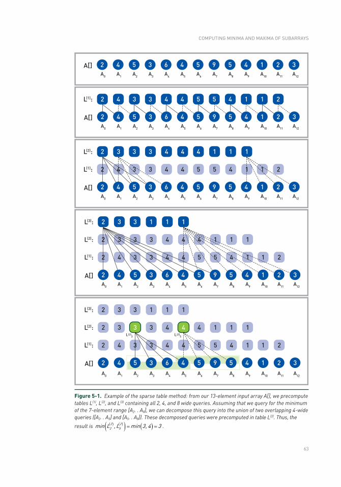
63
Figure 5-1. Example of the sparse table method: from our 13-element input array A[], we precompute tables L(1), L(2), and L(3) containing all 2, 4, and 8 wide queries. Assuming that we query for the minimum of the 7-element range [A2. . A8], we can decompose this query into the union of two overlapping 4-wide queries ([A2. . A5] and [A5. . A8]). These decomposed queries were precomputed in table L(2). Thus, the
result is ( ) ( )( ) ( )2 22 5min L , L min 3, 4 3= = .
COMPUTING MINIMA AND MAxIMA OF SUBARRAyS
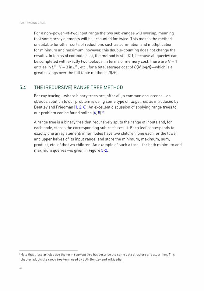
64
For a non–power-of-two input range the two sub-ranges will overlap, meaning that some array elements will be accounted for twice. This makes the method unsuitable for other sorts of reductions such as summation and multiplication; for minimum and maximum, however, this double-counting does not change the results. In terms of compute cost, the method is still O(1) because all queries can be completed with exactly two lookups. In terms of memory cost, there are N − 1 entries in L(1), N − 3 in L(2), etc., for a total storage cost of O(N logN)—which is a great savings over the full table method’s O(N2).
5.4 THE (RECURSIVE) RANGE TREE METHOD
For ray tracing—where binary trees are, after all, a common occurrence—an obvious solution to our problem is using some type of range tree, as introduced by Bentley and Friedman [1, 2, 8]. An excellent discussion of applying range trees to our problem can be found online [4, 5].2
A range tree is a binary tree that recursively splits the range of inputs and, for each node, stores the corresponding subtree’s result. Each leaf corresponds to exactly one array element; inner nodes have two children (one each for the lower and upper halves of its input range) and store the minimum, maximum, sum, product, etc. of the two children. An example of such a tree—for both minimum and maximum queries—is given in Figure 5-2.
2 Note that those articles use the term segment tree but describe the same data structure and algorithm. This chapter adopts the range tree term used by both Bentley and Wikipedia.
RAY TRACING GEMS
65
Given such a range tree, querying over any range [lo, hi] requires finding the set of nodes that exactly spans the input range. The following simple recursive algorithm performs this query:
1 RangeTree::query(node,[lo,hi])
2 if (node.indexRange does not overlap [lo,hi])
3 /* Case 1: node completely outside query range -> ignore. */
4 return empty range
Figure 5-2. Illustration of the recursive range tree method. Given input array A (top), we compute a binary tree (middle) where each node stores the minimum and maximum of its corresponding leaf nodes. Our recursive traversal for a query range (bottom) uses all three cases from the pseudocode: gray nodes recurse into both children (case 3), green nodes with dark outlines get counted and terminate (case 2), and blue nodes with dashed outlines lie outside the range (case 1).
COMPUTING MINIMA AND MAxIMA OF SUBARRAyS
66
5 if (node.indexRange is inside [lo,hi])
6 /* Case 2: node completely inside query range -> use it. */
7 return node, valueRange
8 /* Case 3: partial overlap -> recurse into children, & merge. */
9 return merge(query(node.leftChild,[lo,hi]),
10 query(node.rightChild,[lo,hi])
11
Range trees require only linear storage and preprocessing time, which can be integer factors less than the sparse table method. On the downside, queries no longer occur in constant time, but instead have O(logN) complexity. Even worse, recursive queries can incur relatively high “implementation constants” (especially on SIMD or SPMD architectures), even with careful data layouts and when avoiding pointer chasing.
5.5 ITERATIVE RANGE TREE QUERIES
In practice, the main cost of range tree queries lies not in their O(logN) complexity, but rather in the high implementation constants for recursion. As such, an iterative method would be highly preferable.
To derive such a method, we now look at a logical range tree from the bottom up, as a successive merging of respectively next-finer levels. On the finest level L(0), we have the N0 = N original array values, ( )
i iL A0 = . On the next level, we compute the min or max of each (complete) pair of values from the previous level, meaning there are N1 = ⌊N0/2⌋ values of ( ) ( ) ( )( )i i iL f L ,L1 0 0
2 2 1+= , where f could be min or max; level 2 has N2 = ⌊N1/2⌋ such merged pairs from L(1), and so on. For non–power-of-two arrays, some of the Ni can be odd, meaning some nodes will not have a parent; this is somewhat counterintuitive, but for our traversal algorithm it will turn out just fine.
See Figure 5-3 for an illustration of the resulting data structure, which forms a series of binary trees (one tree if N is a power of two, and more otherwise). A node n on any level L is the root of a binary tree representing all array values within this (sub)tree.
RAY TRACING GEMS
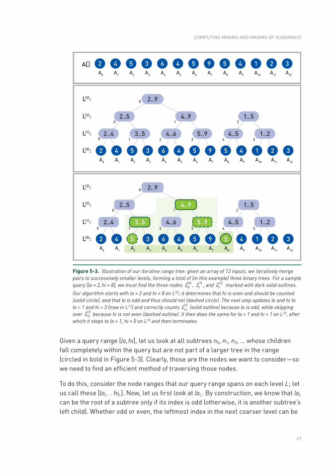
67
Given a query range [lo, hi], let us look at all subtrees n0, n1, n2, … whose children fall completely within the query but are not part of a larger tree in the range (circled in bold in Figure 5-3). Clearly, those are the nodes we want to consider—so we need to find an efficient method of traversing those nodes.
To do this, consider the node ranges that our query range spans on each level L; let us call these [loL. . hiL]. Now, let us first look at loL. By construction, we know that loL can be the root of a subtree only if its index is odd (otherwise, it is another subtree’s left child). Whether odd or even, the leftmost index in the next coarser level can be
Figure 5-3. Illustration of our iterative range tree: given an array of 13 inputs, we iteratively merge pairs to successively smaller levels, forming a total of (in this example) three binary trees. For a sample query [lo = 2, hi = 8], we must find the three nodes ( )0
8L , ( )11L , and ( )2
1L marked with dark solid outlines.
Our algorithm starts with lo = 2 and hi = 8 on L(0); it determines that hi is even and should be counted (solid circle), and that lo is odd and thus should not (dashed circle). The next step updates lo and hi to lo = 1 and hi = 3 (now in L(1)) and correctly counts ( )1
loL (solid outline) because lo is odd, while skipping over ( )1
hiL because hi is not even (dashed outline). It then does the same for lo = 1 and hi = 1 on L(2), after which it steps to lo = 1, hi = 0 on L(3) and then terminates.
COMPUTING MINIMA AND MAxIMA OF SUBARRAyS
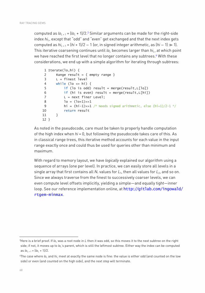
68
computed as loL + 1 = (loL + 1)/2.3 Similar arguments can be made for the right-side index hiL, except that “odd” and “even” get exchanged and that the next index gets computed as hiL + 1 = (hi + 1)/2 − 1 (or, in signed integer arithmetic, as (hi − 1) ≫ 1). This iterative coarsening continues until loL becomes larger than hiL, at which point we have reached the first level that no longer contains any subtrees.4 With these considerations, we end up with a simple algorithm for iterating through subtrees:
1 Iterate(lo,hi)
2 Range result = empty range
3 L = finest level
4 while (lo <= hi)
5 if (lo is odd) result = merge(result,L[lo])
6 if (hi is even) result = merge(result,L[hi])
7 L = next finer Level;
8 lo = (lo+1)>>1
9 hi = (hi-1)>>1 /* Needs signed arithmetic, else (hi+1)/2-1 */
10 return result
11
12
As noted in the pseudocode, care must be taken to properly handle computation of the high index when hi = 0, but following the pseudocode takes care of this. As in classical range trees, this iterative method accounts for each value in the input range exactly once and could thus be used for queries other than minimum and maximum.
With regard to memory layout, we have logically explained our algorithm using a sequence of arrays (one per level). In practice, we can easily store all levels in a single array that first contains all N1 values for L1, then all values for L2, and so on. Since we always traverse from the finest to successively coarser levels, we can even compute level offsets implicitly, yielding a simple—and equally tight—inner loop. See our reference implementation online, at http://gitlab.com/ingowald/rtgem-minmax.
3 Here is a brief proof. If loL was a root node in L then it was odd, so this moves it to the next subtree on the right side; if not, it moves up to loL’s parent, which is still the leftmost subtree. Either way the index can be computed as loL + 1 = (loL + 1)/2.
4 The case where loL and hiL meet at exactly the same node is fine: the value is either odd (and counted on the low side) or even (and counted on the high side), and the next step will terminate.
RAY TRACING GEMS
69
5.6 RESULTS
Theoretically, our iterative method has the same storage complexity, O(N), and computational complexity, O(logN), as the classical range tree method. However, its memory layout is much simpler, and the time constant for querying is significantly lower than in any recursive implementation. In fact, with our sample code this iterative version is almost as fast as the O(1) sparse table method, except for tables with at least hundreds of thousands of elements—while using significantly less memory.
For example, using an array with 4k elements and randomly chosen query endpoints lo and hi, the iterative method is only about 5% slower than the sparse table method, at 10× lower memory usage. For a larger 100k-element table, the speed difference increases to roughly 30%, but at 15×; lower memory usage. While already a interesting trade-off, it is worth noting that randomly chosen query endpoints are close to the iterative method’s worst case: since iteration count is logarithmic in ∣hi-lo∣, “narrower” queries actually run faster than very wide ones performed by uniformly chosen lo and hi values. For example, if we limit the query values to ∣hi-lo∣ ≤ N , the iterative method on the 100k-element array changes from 30% slower to 15% faster than the sparse table method (at 15× less memory)
5.7 SUMMARy
In this chapter, we have summarized four methods for computing the minima and maxima for any sub-range of an array of numbers. The naive full table method is the easiest to implement and is fast in query—but suffers from O(N2) storage and recomputation cost, which limit its usefulness. The sparse table method is slightly more complex but significantly reduces the memory overhead, while retaining the O(1) query complexity. The recursive range tree method reduces this memory overhead even more (to O(N)), but at the cost of a significantly higher query complexity—not only theoretically (at O(logN)) but also in actual implementation constants. Finally, our iterative range tree retains the low memory overhead of range trees, uses a simpler memory layout, and converts the recursive query into a tight iterative loop. Though asymptotically still O(logN), in practice its queries perform similar to the O(1) sparse table method, at lower memory consumption. Overall, this makes the iterative method our favorite, in particular since both precomputation code and query code are surprisingly simple.
Sample code for the sparse table and the iterative range tree methods are available online, at https://gitlab.com/ingowald/rtgem-minmax.
COMPUTING MINIMA AND MAxIMA OF SUBARRAyS
70
REFERENCES
[1] Bentley, J. L., and Friedman, J. H. A Survey of Algorithms and Data Structures for Range Searching. http://www.slac.stanford.edu/cgi-wrap/getdoc/slac- pub- 2189.pdf, 1978.
[2] Bentley, J. L., and Friedman, J. H. Algorithms and Data Structures for Range Searching. ACM Computing Surveys 11, 4 (1979), 397–409.
[3] Crow, F. Summed-Area Tables for Texture Mapping. Computer Graphics (SIGGRAPH) 18, 3 (1984), 207—212.
[4] GeeksForGeeks. Min-Max Range Queries in Array. https://www.geeksforgeeks.org/min-max-range-queries-array/. Last accessed December 7, 2018.
[5] GeeksForGeeks. Segment Tree: Set 2 (Range Minimum Query). https://www.geeksforgeeks.org/segment-tree-set-1-range-minimum-query/. Last accessed December 7, 2018.
[6] GeeksForGeeks. Sparse Table. https://www.geeksforgeeks.org/sparse-table/. Last accessed December 7, 2018.
[7] Wald, I., Johnson, G. P., Amstutz, J., Brownlee, C., Knoll, A., Jeffers, J. L., Guenther, J., and Navratil, P. OSPRay—A CPU Ray Tracing Framework for Scientific Visualization. IEEE Transactions on Visualization 23, 1 (2017), 931–940.
[8] Wikipedia. Range Tree. https://en.wikipedia.org/wiki/Range_tree. Last accessed December 7, 2018.
[9] Wikipedia. Summed-Area Table. https://en.wikipedia.org/wiki/Summed- area_table. Last accessed December 7, 2018.
Open Access This chapter is licensed under the terms of the Creative Commons Attribution-NonCommercial-NoDerivatives 4.0 International License (http://creativecommons.org/licenses/by-nc-nd/4.0/), which permits any noncommercial use, sharing, distribution and
reproduction in any medium or format, as long as you give appropriate credit to the original author(s) and the source, provide a link to the Creative Commons license and indicate if you modified the licensed material. you do not have permission under this license to share adapted material derived from this chapter or parts of it.
The images or other third party material in this chapter are included in the chapter's Creative Commons license, unless indicated otherwise in a credit line to the material. If material is not included in the chapter's Creative Commons license and your intended use is not permitted by statutory regulation or exceeds the permitted use, you will need to obtain permission directly from the copyright holder.
RAY TRACING GEMS
PART II
INTERSECTIONS AND EFFICIENCY

75
PART II
Intersections and Efficiency
Ray tracing has many useful properties, but eventually, the two by which people seem most captivated are its elegance and simplicity. New rendering algorithms and effects can be added by just tracing some rays. New surface primitives can be added by simply specifying their bounding box and intersection programs. Parallelism is often “embarrassingly” simple to achieve.
As with everything else, all of this is profoundly true—until it is not. Any one of the above properties is true in principle, but only until one hits “the good, the bad, and the ugly” cases—namely, those where the default find-the-intersection interface is no longer sufficient; where limited floating precision messes up nice mathematical solutions; where “edge cases” such as multiple coplanar surfaces, “unreasonably” small or faraway geometry, or grossly uneven costs per pixel rear their ugly heads. Such challenges are tempting to gloss over as pathological cases, but in practice, they can only be ignored at one’s peril.
Chapter 6, “A Fast and Robust Method for Avoiding Self-Intersection,” discusses how rays originating at a surface intersect the surface itself. It presents a solution that is easy to implement, yet battle-proven in a production ray tracer.
Chapter 7, “Precision Improvements for Ray/Sphere Intersection,” looks at how quickly limited floating-point precision can interfere with the root finding done in ray/sphere intersection and how this can be fixed in a numerically stable way that can also carry beyond spheres.
Chapter 8, “Cool Patches: A Geometric Approach to Ray/Bilinear Patch Intersections,” describes a new geometric primitive that allows for easy handling of arbitrary (i.e., nonplanar) quadrilateral patches without the need to split them into two triangles, while remaining both numerically robust and fast.
Chapter 9, “Multi-Hit Ray Tracing in DXR,” looks at the case where applications need to efficiently and robustly find not just “the”—but rather multiple—successive intersections along a ray, as well as looks into how to add that functionality on top of the existing DXR API.

76
Finally, Chapter 10, “A Simple Load-Balancing Scheme with High Scaling Efficiency,” proposes a straightforward yet effective method of achieving nicely work-balanced image-space parallelization. It works even in the presence of wildly differing costs per pixel, for which naive approaches tend to break down.
Having had to deal with literally every one of these chapters’ topics in the past, I am particularly excited to present this part’s selection of chapters. I do hope that they will provide insight—and ideally, reference solutions—for those ray tracers that are yet to be written.
Ingo Wald
77© NVIDIA 2019 E. Haines, T. Akenine-Möller (eds.), Ray Tracing Gems, https://doi.org/10.1007/978-1-4842-4427-2_6
CHAPTER 6
A Fast and Robust Method for Avoiding Self- IntersectionCarsten Wächter and Nikolaus Binder NVIDIA
ABSTRACT
We present a solution to avoid self-intersections in ray tracing that is more robust than current common practices while introducing minimal overhead and requiring no parameter tweaking.
6.1 INTRODUCTION
Ray and path tracing simulations construct light paths by starting at the camera or the light sources and intersecting rays with the scene geometry. As objects are hit, new rays are generated on these surfaces to continue the paths. In theory, these new rays will not yield an intersection with the same surface again, as intersections at a distance of zero are excluded by the intersection algorithm. In practice, however, the finite floating-point precision used in the actual implementation often leads to false positive results, known as self-intersections, creating artifacts such as shadow acne, where the surface sometimes improperly shadows itself.
The most widespread solutions to work around the issue are not robust enough to handle a variety of common production content and may even require manual parameter tweaking on a per-scene basis. Alternatively, a thorough numerical analysis of the source of the numerical imprecision allows for robust handling. However, this comes with a considerable performance overhead and requires source access to the underlying implementation of the ray/surface intersection routine, which is not possible in some software APIs and especially not with hardware-accelerated technology, e.g., NVIDIA RTX.
In this chapter we present a method that is reasonably robust, does not require any parameter tweaking, and at the same time introduces minimal overhead, making it suitable for real-time applications as well as offline rendering.
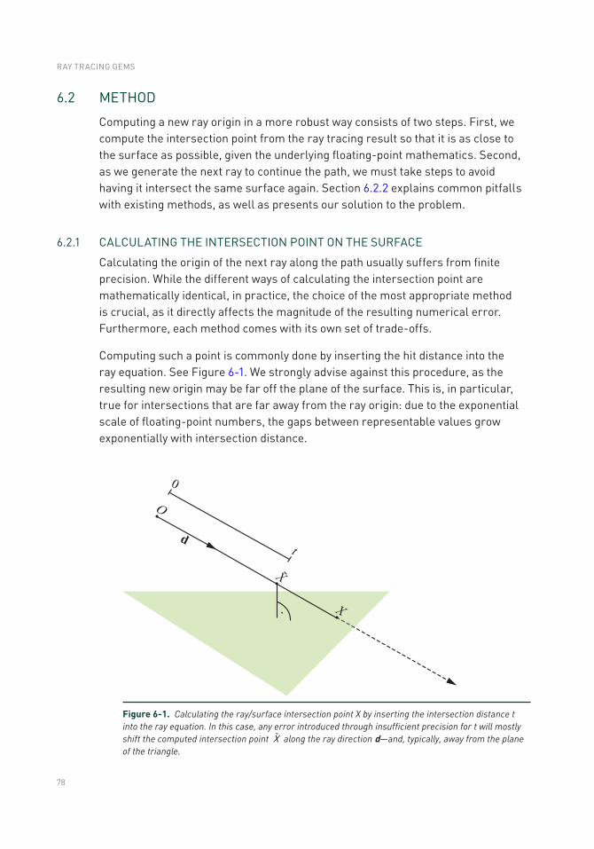
78
6.2 METHOD
Computing a new ray origin in a more robust way consists of two steps. First, we compute the intersection point from the ray tracing result so that it is as close to the surface as possible, given the underlying floating-point mathematics. Second, as we generate the next ray to continue the path, we must take steps to avoid having it intersect the same surface again. Section 6.2.2 explains common pitfalls with existing methods, as well as presents our solution to the problem.
6.2.1 CALCULATING THE INTERSECTION POINT ON THE SURFACE
Calculating the origin of the next ray along the path usually suffers from finite precision. While the different ways of calculating the intersection point are mathematically identical, in practice, the choice of the most appropriate method is crucial, as it directly affects the magnitude of the resulting numerical error. Furthermore, each method comes with its own set of trade-offs.
Computing such a point is commonly done by inserting the hit distance into the ray equation. See Figure 6-1. We strongly advise against this procedure, as the resulting new origin may be far off the plane of the surface. This is, in particular, true for intersections that are far away from the ray origin: due to the exponential scale of floating-point numbers, the gaps between representable values grow exponentially with intersection distance.
t
O
d
0
X
X
Figure 6-1. Calculating the ray/surface intersection point X by inserting the intersection distance t into the ray equation. In this case, any error introduced through insufficient precision for t will mostly shift the computed intersection point X along the ray direction d—and, typically, away from the plane of the triangle.
RAY TRACING GEMS
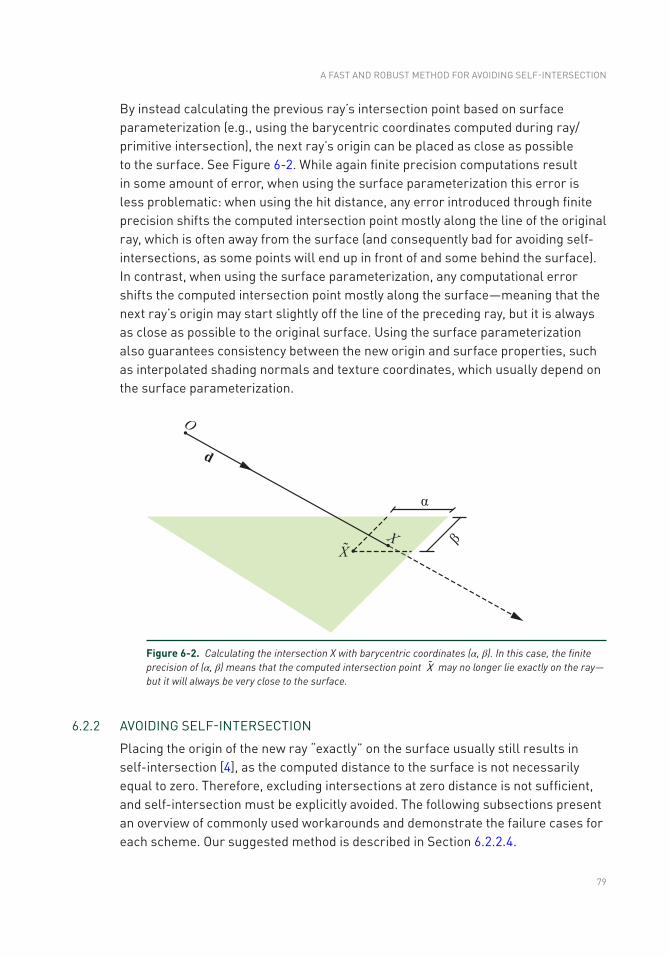
79
By instead calculating the previous ray’s intersection point based on surface parameterization (e.g., using the barycentric coordinates computed during ray/primitive intersection), the next ray’s origin can be placed as close as possible to the surface. See Figure 6-2. While again finite precision computations result in some amount of error, when using the surface parameterization this error is less problematic: when using the hit distance, any error introduced through finite precision shifts the computed intersection point mostly along the line of the original ray, which is often away from the surface (and consequently bad for avoiding self-intersections, as some points will end up in front of and some behind the surface). In contrast, when using the surface parameterization, any computational error shifts the computed intersection point mostly along the surface—meaning that the next ray’s origin may start slightly off the line of the preceding ray, but it is always as close as possible to the original surface. Using the surface parameterization also guarantees consistency between the new origin and surface properties, such as interpolated shading normals and texture coordinates, which usually depend on the surface parameterization.
Figure 6-2. Calculating the intersection X with barycentric coordinates (α, β). In this case, the finite precision of (α, β) means that the computed intersection point X may no longer lie exactly on the ray—but it will always be very close to the surface.
6.2.2 AVOIDING SELF-INTERSECTION
Placing the origin of the new ray “exactly” on the surface usually still results in self- intersection [4], as the computed distance to the surface is not necessarily equal to zero. Therefore, excluding intersections at zero distance is not sufficient, and self-intersection must be explicitly avoided. The following subsections present an overview of commonly used workarounds and demonstrate the failure cases for each scheme. Our suggested method is described in Section 6.2.2.4.
A FAST AND ROBUST METHOD FOR AVOIDING SELF- INTERSECTION
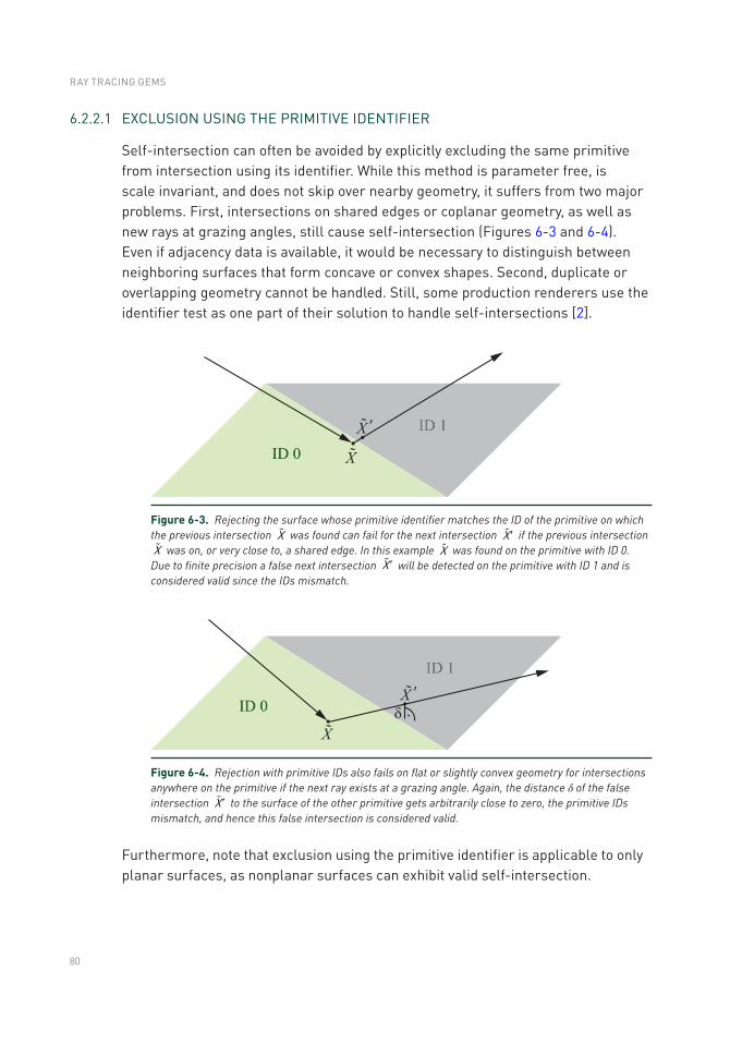
80
6.2.2.1 EXCLUSION USING THE PRIMITIVE IDENTIFIER
Self-intersection can often be avoided by explicitly excluding the same primitive from intersection using its identifier. While this method is parameter free, is scale invariant, and does not skip over nearby geometry, it suffers from two major problems. First, intersections on shared edges or coplanar geometry, as well as new rays at grazing angles, still cause self-intersection (Figures 6-3 and 6-4). Even if adjacency data is available, it would be necessary to distinguish between neighboring surfaces that form concave or convex shapes. Second, duplicate or overlapping geometry cannot be handled. Still, some production renderers use the identifier test as one part of their solution to handle self-intersections [2].
Figure 6-3. Rejecting the surface whose primitive identifier matches the ID of the primitive on which the previous intersection X was found can fail for the next intersection X ¢ if the previous intersection X was on, or very close to, a shared edge. In this example X was found on the primitive with ID 0. Due to finite precision a false next intersection X ¢ will be detected on the primitive with ID 1 and is considered valid since the IDs mismatch.
Figure 6-4. Rejection with primitive IDs also fails on flat or slightly convex geometry for intersections anywhere on the primitive if the next ray exists at a grazing angle. Again, the distance δ of the false intersection X ¢ to the surface of the other primitive gets arbitrarily close to zero, the primitive IDs mismatch, and hence this false intersection is considered valid.
Furthermore, note that exclusion using the primitive identifier is applicable to only planar surfaces, as nonplanar surfaces can exhibit valid self-intersection.
RAY TRACING GEMS
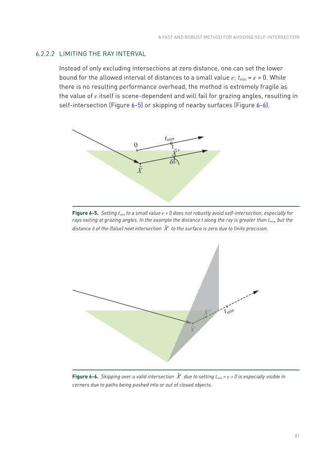
81
6.2.2.2 LIMITING THE RAY INTERVAL
Instead of only excluding intersections at zero distance, one can set the lower bound for the allowed interval of distances to a small value ε: tmin = ε > 0. While there is no resulting performance overhead, the method is extremely fragile as the value of ε itself is scene- dependent and will fail for grazing angles, resulting in self-intersection (Figure 6-5) or skipping of nearby surfaces (Figure 6-6).
Figure 6-5. Setting tmin to a small value ε > 0 does not robustly avoid self- intersection, especially for rays exiting at grazing angles. In the example the distance t along the ray is greater than tmin, but the
distance δ of the (false) next intersection X ¢ to the surface is zero due to finite precision.
X
X ' tmin
X
XX''
Figure 6-6. Skipping over a valid intersection X ¢ due to setting tmin = ε > 0 is especially visible in
corners due to paths being pushed into or out of closed objects.
A FAST AND ROBUST METHOD FOR AVOIDING SELF- INTERSECTION
82
6.2.2.3 OFFSETTING ALONG THE SHADING NORMAL OR THE OLD RAY DIRECTION
Offsetting the ray origin along the shading normal is similar to setting the lower bound of a ray tmin = ε > 0 and features the same failure cases, as this vector is not necessarily perpendicular to the surface (due to interpolation or variation computed from bump or normal maps).
Shifting the new ray origin along the old ray direction will again suffer from similar issues.
6.2.2.4 ADAPTIVE OFFSETTING ALONG THE GEOMETRIC NORMAL
As could be seen in the previous subsections, only the geometric normal, being orthogonal to the surface by design, can feature the smallest offset, dependent on the distance to the intersection point, to escape self-intersection while not introducing any of the mentioned shortcomings. The next step will focus on how to compute the offset to place the ray origin along it.
Using any offset of fixed length ε is not scale invariant, and thus not parameter free, and will also not work for intersections at varying magnitudes of distance. Therefore, analyzing the error of the floating-point calculations to compute the intersection point using barycentric coordinates reveals that the distance of the intersection to the plane of the surface is proportional to the distance from the origin (0,0,0). At the same time the size of the surface also influences the error and even becomes dominant for triangles very close to the origin (0,0,0). Using only normalized ray directions removes the additional impact of the length of the ray on the numerical error. The experimental results in Figure 6-7 for random triangles illustrate this behavior: We calculate the average and maximum distance of the computed intersection point to 10 million triangles with edge lengths between 2−16 and 222. As the resulting point can be located on either side of the actual plane, a robust offset needs to be at least as large as the maximum distance.
RAY TRACING GEMS
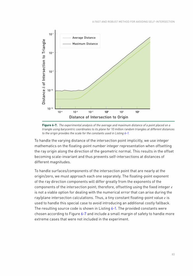
83
Figure 6-7. The experimental analysis of the average and maximum distance of a point placed on a triangle using barycentric coordinates to its plane for 10 million random triangles at different distances to the origin provides the scale for the constants used in Listing 6-1.
To handle the varying distance of the intersection point implicitly, we use integer mathematics on the floating-point number integer representation when offsetting the ray origin along the direction of the geometric normal. This results in the offset becoming scale-invariant and thus prevents self-intersections at distances of different magnitudes.
To handle surfaces/components of the intersection point that are nearly at the origin/zero, we must approach each one separately. The floating-point exponent of the ray direction components will differ greatly from the exponents of the components of the intersection point; therefore, offsetting using the fixed integer ε is not a viable option for dealing with the numerical error that can arise during the ray/plane intersection calculations. Thus, a tiny constant floating-point value ε is used to handle this special case to avoid introducing an additional costly fallback. The resulting source code is shown in Listing 6-1. The provided constants were chosen according to Figure 6-7 and include a small margin of safety to handle more extreme cases that were not included in the experiment.
A FAST AND ROBUST METHOD FOR AVOIDING SELF- INTERSECTION
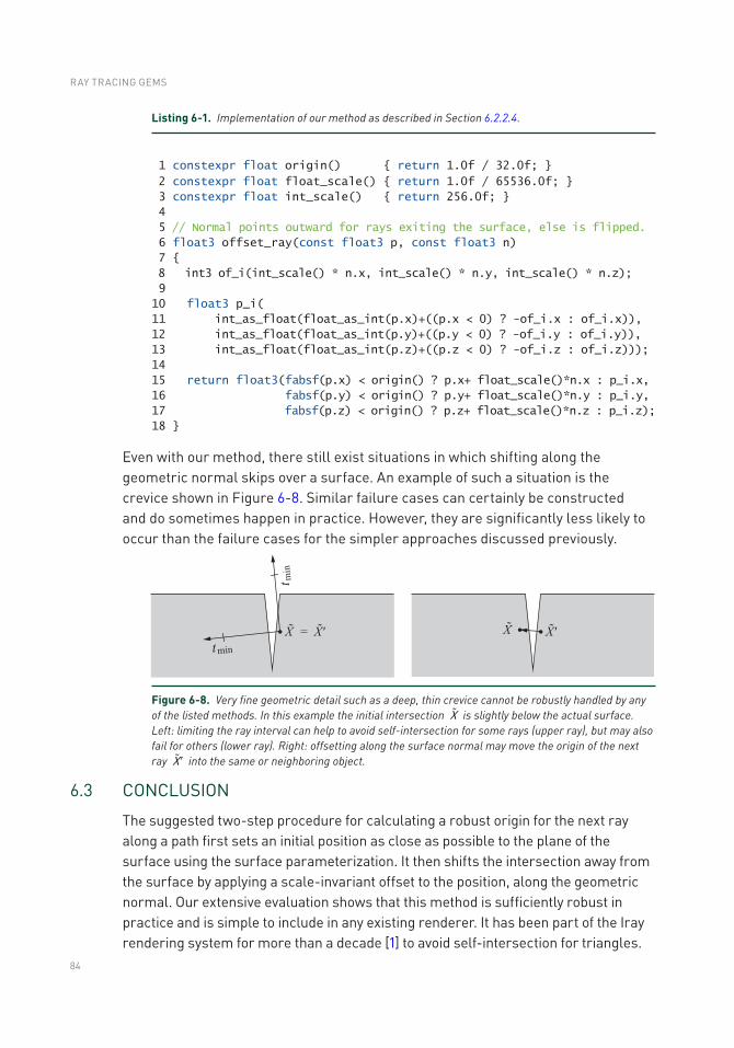
84
6.3 CONCLUSION
The suggested two-step procedure for calculating a robust origin for the next ray along a path first sets an initial position as close as possible to the plane of the surface using the surface parameterization. It then shifts the intersection away from the surface by applying a scale-invariant offset to the position, along the geometric normal. Our extensive evaluation shows that this method is sufficiently robust in practice and is simple to include in any existing renderer. It has been part of the Iray rendering system for more than a decade [1] to avoid self-intersection for triangles.
Figure 6-8. Very fine geometric detail such as a deep, thin crevice cannot be robustly handled by any of the listed methods. In this example the initial intersection X is slightly below the actual surface. Left: limiting the ray interval can help to avoid self-intersection for some rays (upper ray), but may also fail for others (lower ray). Right: offsetting along the surface normal may move the origin of the next ray X ¢ into the same or neighboring object.
Listing 6-1. Implementation of our method as described in Section 6.2.2.4.
1 constexpr float origin() return 1.0f / 32.0f;
2 constexpr float float_scale() return 1.0f / 65536.0f;
3 constexpr float int_scale() return 256.0f;
4
5 // Normal points outward for rays exiting the surface, else is flipped.
6 float3 offset_ray(const float3 p, const float3 n)
7
8 int3 of_i(int_scale() * n.x, int_scale() * n.y, int_scale() * n.z);
9
10 float3 p_i(
11 int_as_float(float_as_int(p.x)+((p.x < 0) ? -of_i.x : of_i.x)),
12 int_as_float(float_as_int(p.y)+((p.y < 0) ? -of_i.y : of_i.y)),
13 int_as_float(float_as_int(p.z)+((p.z < 0) ? -of_i.z : of_i.z)));
14
15 return float3(fabsf(p.x) < origin() ? p.x+ float_scale()*n.x : p_i.x,
16 fabsf(p.y) < origin() ? p.y+ float_scale()*n.y : p_i.y,
17 fabsf(p.z) < origin() ? p.z+ float_scale()*n.z : p_i.z);
18
Even with our method, there still exist situations in which shifting along the geometric normal skips over a surface. An example of such a situation is the crevice shown in Figure 6-8. Similar failure cases can certainly be constructed and do sometimes happen in practice. However, they are significantly less likely to occur than the failure cases for the simpler approaches discussed previously.
RAY TRACING GEMS
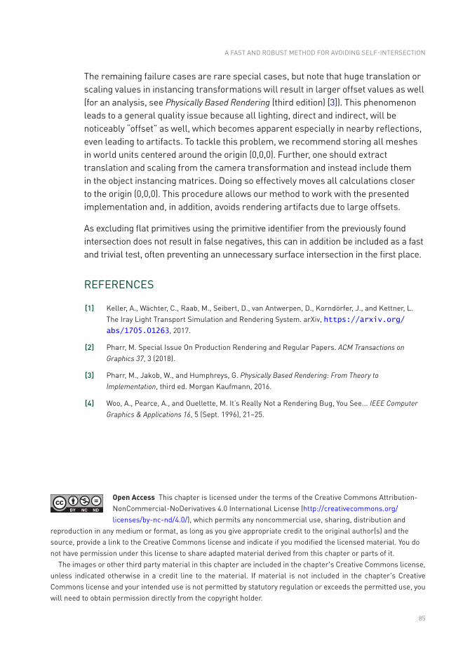
85
The remaining failure cases are rare special cases, but note that huge translation or scaling values in instancing transformations will result in larger offset values as well (for an analysis, see Physically Based Rendering (third edition) [3]). This phenomenon leads to a general quality issue because all lighting, direct and indirect, will be noticeably “offset” as well, which becomes apparent especially in nearby reflections, even leading to artifacts. To tackle this problem, we recommend storing all meshes in world units centered around the origin (0,0,0). Further, one should extract translation and scaling from the camera transformation and instead include them in the object instancing matrices. Doing so effectively moves all calculations closer to the origin (0,0,0). This procedure allows our method to work with the presented implementation and, in addition, avoids rendering artifacts due to large offsets.
As excluding flat primitives using the primitive identifier from the previously found intersection does not result in false negatives, this can in addition be included as a fast and trivial test, often preventing an unnecessary surface intersection in the first place.
REFERENCES
[1] Keller, A., Wächter, C., Raab, M., Seibert, D., van Antwerpen, D., Korndörfer, J., and Kettner, L. The Iray Light Transport Simulation and Rendering System. arXiv, https://arxiv.org/abs/1705.01263, 2017.
[2] Pharr, M. Special Issue On Production Rendering and Regular Papers. ACM Transactions on Graphics 37, 3 (2018).
[3] Pharr, M., Jakob, W., and Humphreys, G. Physically Based Rendering: From Theory to Implementation, third ed. Morgan Kaufmann, 2016.
[4] Woo, A., Pearce, A., and Ouellette, M. It’s Really Not a Rendering Bug, You See... IEEE Computer Graphics & Applications 16, 5 (Sept. 1996), 21–25.
Open Access This chapter is licensed under the terms of the Creative Commons Attribution-NonCommercial-NoDerivatives 4.0 International License (http://creativecommons.org/licenses/by-nc-nd/4.0/), which permits any noncommercial use, sharing, distribution and
reproduction in any medium or format, as long as you give appropriate credit to the original author(s) and the source, provide a link to the Creative Commons license and indicate if you modified the licensed material. You do not have permission under this license to share adapted material derived from this chapter or parts of it.
The images or other third party material in this chapter are included in the chapter's Creative Commons license, unless indicated otherwise in a credit line to the material. If material is not included in the chapter's Creative Commons license and your intended use is not permitted by statutory regulation or exceeds the permitted use, you will need to obtain permission directly from the copyright holder.
A FAST AND ROBUST METHOD FOR AVOIDING SELF- INTERSECTION
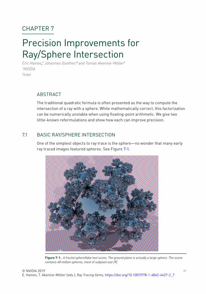
87© NVIDIA 2019 E. Haines, T. Akenine-Möller (eds.), Ray Tracing Gems, https://doi.org/10.1007/978-1-4842-4427-2_7
CHAPTER 7
Precision Improvements for Ray/Sphere IntersectionEric Haines,1 Johannes Günther,2 and Tomas Akenine-Möller1 1NVIDIA 2Intel
ABSTRACT
The traditional quadratic formula is often presented as the way to compute the intersection of a ray with a sphere. While mathematically correct, this factorization can be numerically unstable when using floating-point arithmetic. We give two little-known reformulations and show how each can improve precision.
7.1 BASIC RAY/SPHERE INTERSECTION
One of the simplest objects to ray trace is the sphere—no wonder that many early ray traced images featured spheres. See Figure 7-1.
Figure 7-1. A fractal sphereflake test scene. The ground plane is actually a large sphere. The scene contains 48 million spheres, most of subpixel size [9].
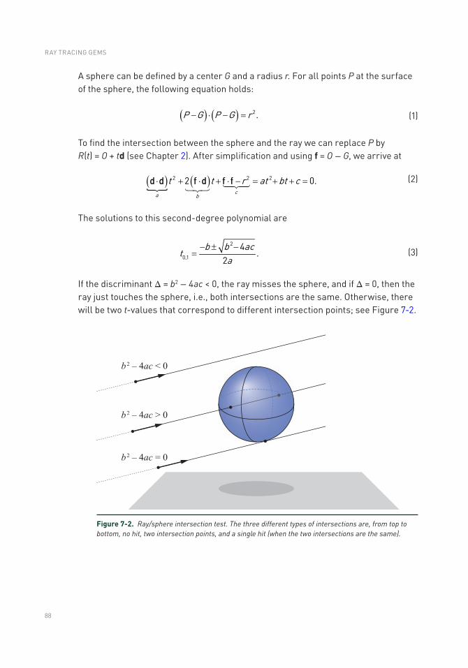
88
A sphere can be defined by a center G and a radius r. For all points P at the surface of the sphere, the following equation holds:
( ) ( )P G P G r 2.- × - = (1)
To find the intersection between the sphere and the ray we can replace P by R(t) = O + td (see Chapter 2). After simplification and using f = O − G, we arrive at
( ) ( )2 2 22 0.
ca b
t t r at bt c× + × + × - = + + =d d f d f f
(2)
The solutions to this second-degree polynomial are
2
0,1
4.
2b b ac
ta
- ± -=
(3)
If the discriminant Δ = b2 − 4ac < 0, the ray misses the sphere, and if Δ = 0, then the ray just touches the sphere, i.e., both intersections are the same. Otherwise, there will be two t-values that correspond to different intersection points; see Figure 7-2.
Figure 7-2. Ray/sphere intersection test. The three different types of intersections are, from top to bottom, no hit, two intersection points, and a single hit (when the two intersections are the same).
RAY TRACING GEMS
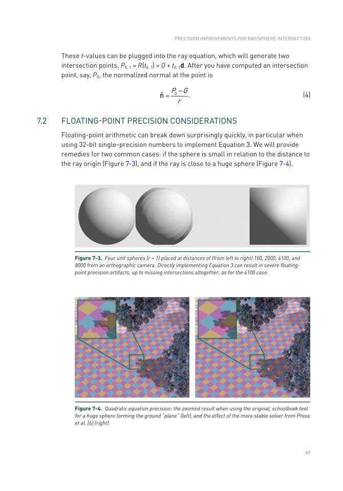
89
These t-values can be plugged into the ray equation, which will generate two intersection points, P0, 1 = R(t0, 1) = O + t0, 1d. After you have computed an intersection point, say, P0, the normalized normal at the point is
-=
P Gr
0ˆ .n
(4)
7.2 FLOATING-POINT PRECISION CONSIDERATIONS
Floating-point arithmetic can break down surprisingly quickly, in particular when using 32-bit single-precision numbers to implement Equation 3. We will provide remedies for two common cases: if the sphere is small in relation to the distance to the ray origin (Figure 7-3), and if the ray is close to a huge sphere (Figure 7-4).
Figure 7-3. Four unit spheres (r = 1) placed at distances of (from left to right) 100, 2000, 4100, and 8000 from an orthographic camera. Directly implementing Equation 3 can result in severe floating-point precision artifacts, up to missing intersections altogether, as for the 4100 case.
Figure 7-4. Quadratic equation precision: the zoomed result when using the original, schoolbook test for a huge sphere forming the ground “plane” (left), and the effect of the more stable solver from Press et al. [6] (right).
PRECISION IMPROVEMENTS FOR RAY/SPHERE INTERSECTION
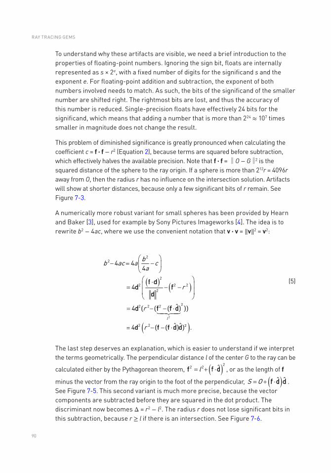
90
To understand why these artifacts are visible, we need a brief introduction to the properties of floating-point numbers. Ignoring the sign bit, floats are internally represented as s × 2e, with a fixed number of digits for the significand s and the exponent e. For floating-point addition and subtraction, the exponent of both numbers involved needs to match. As such, the bits of the significand of the smaller number are shifted right. The rightmost bits are lost, and thus the accuracy of this number is reduced. Single-precision floats have effectively 24 bits for the significand, which means that adding a number that is more than 224 ≈ 107 times smaller in magnitude does not change the result.
This problem of diminished significance is greatly pronounced when calculating the coefficient c = f ⋅ f − r2 (Equation 2), because terms are squared before subtraction, which effectively halves the available precision. Note that f ⋅ f = ‖O − G‖2 is the squared distance of the sphere to the ray origin. If a sphere is more than 212r = 4096r away from O, then the radius r has no influence on the intersection solution. Artifacts will show at shorter distances, because only a few significant bits of r remain. See Figure 7-3.
A numerically more robust variant for small spheres has been provided by Hearn and Baker [3], used for example by Sony Pictures Imageworks [4]. The idea is to rewrite b2 − 4ac, where we use the convenient notation that v ⋅ v = ‖v‖2 = v2:
( ) ( )
( )l
bb ac a ca
r
r
r
2
22
2
2 2 22
2 2 2
2 2
4 44
4
4
4
ˆ
ˆ ˆ .
æ ö- = -ç ÷
è øæ ö×ç ÷= - -ç ÷è ø
= ×
- - ×
- -
f dd f
d
d f f d
d f f d d
2
2
( (
( ( )
)
( )
)
)
=
(5)
The last step deserves an explanation, which is easier to understand if we interpret the terms geometrically. The perpendicular distance l of the center G to the ray can be
calculated either by the Pythagorean theorem, ( )22 2 ˆl= + ×f f d , or as the length of f
minus the vector from the ray origin to the foot of the perpendicular, ( )= + ×S O ˆ ˆf d d . See Figure 7-5. This second variant is much more precise, because the vector components are subtracted before they are squared in the dot product. The discriminant now becomes Δ = r2 − l2. The radius r does not lose significant bits in this subtraction, because r ≥ l if there is an intersection. See Figure 7-6.
RAY TRACING GEMS
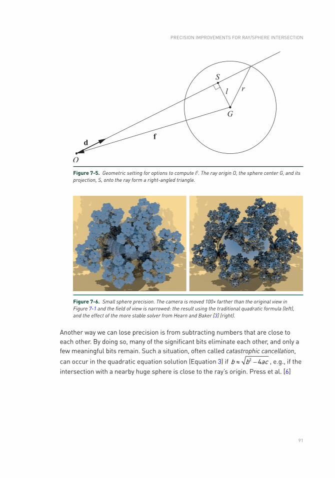
91
Figure 7-5. Geometric setting for options to compute l2. The ray origin O, the sphere center G, and its projection, S, onto the ray form a right-angled triangle.
Figure 7-6. Small sphere precision. The camera is moved 100× farther than the original view in Figure 7-1 and the field of view is narrowed: the result using the traditional quadratic formula (left), and the effect of the more stable solver from Hearn and Baker [3] (right).
Another way we can lose precision is from subtracting numbers that are close to each other. By doing so, many of the significant bits eliminate each other, and only a few meaningful bits remain. Such a situation, often called catastrophic cancellation,
can occur in the quadratic equation solution (Equation 3) if b b ac2 4» - , e.g., if the intersection with a nearby huge sphere is close to the ray’s origin. Press et al. [6]
PRECISION IMPROVEMENTS FOR RAY/SPHERE INTERSECTION
92
give a more stable version, used in the pbrt renderer [5] and other systems. The key observation is that catastrophic cancellation happens only for one of the two quadratic solutions, depending on the sign of b. We can compute that solution with
higher precision using the identity ct ta0 1 = :
( )( )ctq q b b b acqta
02
1
,1where sign 4 .2
,
ì=ïï = - + -í
ï =ïî
(6)
Here, sign is the sign function, which returns 1 if the argument is greater than zero and −1 otherwise. See Figure 7-4 for the effect.
These two methods can be used together, as they are independent of each other. The first computes the discriminant in a more stable way, and the second then decides how best to use this discriminant to find the distances. The quadratic equation can also be solved without need for values such as “4” by reformulating the b value. The unified solution, along with other simplifications, is
= ×a ,d d (7)
¢ = - ×b ,f d (8)
æ öD = - +ç
¢÷
è ø
bra
22 ,f d (9)
where Δ is the discriminant. If Δ is not negative, the ray hits the sphere, so then b′ and Δ are used to find the two distances. We then compute c = f2 − r2 as before to get
( )ctq q b b aqta
0
1
,where sign .
,
¢
ì=ïï = + Dí
ï =
¢
ïî
(10)
If we can assume that the ray direction is normalized, then a = 1 and the solutions get slightly simpler.
RAY TRACING GEMS
93
Earlier exits and shortcuts are also possible if the situation warrants. For example, c is positive when the ray starts outside the sphere and negative when inside, which can tell us whether to return t0 or t1, respectively. If b′ is a negative value, then the center of the sphere is behind the ray, so if it is also the case that c is positive, the ray must miss the sphere [2].
There is, then, no single best way to intersect a sphere with a ray. For example, if you know your application is unlikely to have the camera close to large spheres, you might not want to use the method by Press et al., as it adds a bit of complication.
7.3 RELATED RESOURCES
Code implementing these variant formulations is available on Github [8]. Ray intersectors such as those implemented in shaders in Shadertoy [7] are another way to experiment with various formulations.
ACKNOWLEDGMENTS
Thanks to Stefan Jeschke who pointed out the Hearn and Baker small spheres test, Chris Wyman and the Falcor team [1] for creating the framework on which the sphereflake demo was built, and John Stone for independent confirmation of results.
REFERENCES
[1] Benty, N., Yao, K.-H., Foley, T., Kaplanyan, A. S., Lavelle, C., Wyman, C., and Vijay, A. The Falcor Rendering Framework. https://github.com/NVIDIAGameWorks/Falcor, July 2017.
[2] Haines, E. Essential Ray Tracing Algorithms. In An Introduction to Ray Tracing, A. S. Glassner, Ed. Academic Press Ltd., 1989, pp. 33–77.
[3] Hearn, D. D., and Baker, M. P. Computer Graphics with OpenGL, third ed. Pearson, 2004.
[4] Kulla, C., Conty, A., Stein, C., and Gritz, L. Sony Pictures Imageworks Arnold. ACM Transactions on Graphics 37, 3 (2018), 29:1–29:18.
[5] Pharr, M., Jakob, W., and Humphreys, G. Physically Based Rendering: From Theory to Implementation, third ed. Morgan Kaufmann, 2016.
[6] Press, W. H., Teukolsky, S. A., Vetterling, W. T., and Flannery, B. P. Numerical Recipes: The Art of Scientific Computing, third ed. Cambridge University Press, 2007.
PRECISION IMPROVEMENTS FOR RAY/SPHERE INTERSECTION

94
[7] Quílez, I. Intersectors. http://www.iquilezles.org/www/articles/intersectors/intersectors.htm, 2018.
[8] Wyman, C. A Gentle Introduction to DirectX Raytracing, August 2018. Original code linked from http://cwyman.org/code/dxrTutors/dxr_tutors.md.html; newer code available via https://github.com/NVIDIAGameWorks/GettingStartedWithRTXRayTracing. Last accessed November 12, 2018.
[9] Wyman, C., and Haines, E. Getting Started with RTX Ray Tracing. https://github.com/NVIDIAGameWorks/GettingStartedWithRTXRayTracing, October 2018.
Open Access This chapter is licensed under the terms of the Creative Commons Attribution-NonCommercial-NoDerivatives 4.0 International License (http://creativecommons.org/licenses/by-nc-nd/4.0/), which permits any noncommercial use, sharing, distribution and
reproduction in any medium or format, as long as you give appropriate credit to the original author(s) and the source, provide a link to the Creative Commons license and indicate if you modified the licensed material. You do not have permission under this license to share adapted material derived from this chapter or parts of it.
The images or other third party material in this chapter are included in the chapter's Creative Commons license, unless indicated otherwise in a credit line to the material. If material is not included in the chapter's Creative Commons license and your intended use is not permitted by statutory regulation or exceeds the permitted use, you will need to obtain permission directly from the copyright holder.
RAY TRACING GEMS
95© NVIDIA 2019 E. Haines, T. Akenine-Möller (eds.), Ray Tracing Gems, https://doi.org/10.1007/978-1-4842-4427-2_8
CHAPTER 8
Cool Patches: A Geometric Approach to Ray/Bilinear Patch IntersectionsAlexander Reshetov NVIDIA
ABSTRACT
We find intersections between a ray and a nonplanar bilinear patch using simple geometrical constructs. The new algorithm improves the state of the art performance by over 6× and is faster than approximating a patch with two triangles.
8.1 INTRODUCTION AND PRIOR ART
Computer graphics strives to visualize the real world in all its abundant shapes and colors. Usually, curved surfaces are tessellated to take advantage of the processing power of modern GPUs. The two main rendering techniques—rasterization and ray tracing—now both support hardware-optimized triangle primitives [5, 19]. However, tessellation has its drawbacks, requiring, for example, a significant memory footprint to accurately represent the complex shapes.
Content creation tools instead tend to use higher-order surfaces due to their simplicity and expressive power. Such surfaces can be directly tessellated and rasterized in the DirectX 11 hardware pipeline [7, 17]. As of today, modern GPUs do not natively support ray tracing of nonplanar primitives.
We revisit ray tracing of higher-order primitives, trying to find a balance between the simplicity of triangles and the richness of such smooth shapes as subdivision surfaces [3, 16], NURBS [1], and Bézier patches [2].
Commonly, third (or higher) degree representations are used to generate a smooth surface with continuous normals. Peters [21] proposed a smooth surface jointly modeled by quadratic and cubic patches. For a height field, a C1 quadratic interpolation of an arbitrary triangular mesh can be achieved by subdividing each triangle into 24 triangles [28]. The additional control points are needed to interpolate the given vertex positions and derivatives. For a surface consisting only of quadratic or piecewise-linear patches, the appearance of smoothness can be achieved with Phong shading [22] by interpolating vertex normals, which is
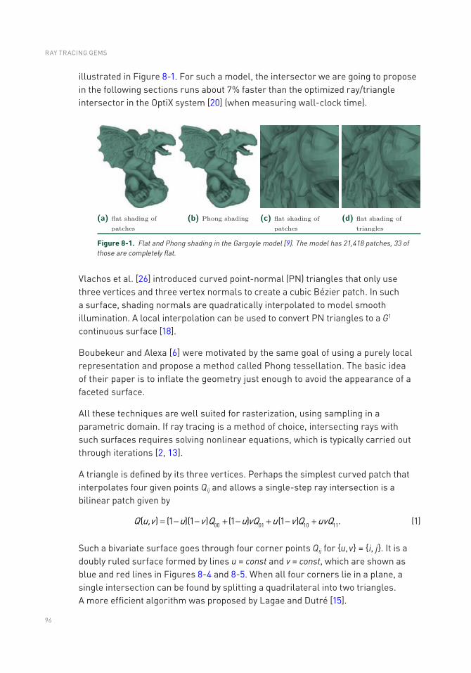
96
illustrated in Figure 8-1. For such a model, the intersector we are going to propose in the following sections runs about 7% faster than the optimized ray/triangle intersector in the OptiX system [20] (when measuring wall-clock time).
Figure 8-1. Flat and Phong shading in the Gargoyle model [9]. The model has 21,418 patches, 33 of those are completely flat.
Vlachos et al. [26] introduced curved point-normal (PN) triangles that only use three vertices and three vertex normals to create a cubic Bézier patch. In such a surface, shading normals are quadratically interpolated to model smooth illumination. A local interpolation can be used to convert PN triangles to a G1 continuous surface [18].
Boubekeur and Alexa [6] were motivated by the same goal of using a purely local representation and propose a method called Phong tessellation. The basic idea of their paper is to inflate the geometry just enough to avoid the appearance of a faceted surface.
All these techniques are well suited for rasterization, using sampling in a parametric domain. If ray tracing is a method of choice, intersecting rays with such surfaces requires solving nonlinear equations, which is typically carried out through iterations [2, 13].
A triangle is defined by its three vertices. Perhaps the simplest curved patch that interpolates four given points Qij and allows a single-step ray intersection is a bilinear patch given by
Q u,v u v Q u vQ u v Q uvQ00 01 10 11( ) (1 )(1 ) (1 ) (1 ) .= - - + - + - + (1)
Such a bivariate surface goes through four corner points Qij for u, v = i, j. It is a doubly ruled surface formed by lines u = const and v = const, which are shown as blue and red lines in Figures 8-4 and 8-5. When all four corners lie in a plane, a single intersection can be found by splitting a quadrilateral into two triangles. A more efficient algorithm was proposed by Lagae and Dutré [15].
RAY TRACING GEMS
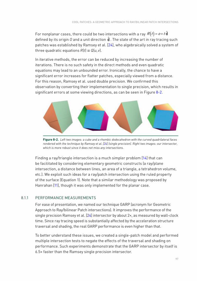
97
For nonplanar cases, there could be two intersections with a ray ( ) = +R t o t d defined by its origin O and a unit direction d . The state of the art in ray tracing such patches was established by Ramsey et al. [24], who algebraically solved a system of three quadratic equations R(t) ≡ Q(u, v).
In iterative methods, the error can be reduced by increasing the number of iterations. There is no such safety in the direct methods and even quadratic equations may lead to an unbounded error. Ironically, the chance to have a significant error increases for flatter patches, especially viewed from a distance. For this reason, Ramsey et al. used double precision. We confirmed this observation by converting their implementation to single precision, which results in significant errors at some viewing directions, as can be seen in Figure 8-2.
Figure 8-2. Left two images: a cube and a rhombic dodecahedron with the curved quadrilateral faces rendered with the technique by Ramsey et al. [24] (single precision). Right two images: our intersector, which is more robust since it does not miss any intersections.
Finding a ray/triangle intersection is a much simpler problem [14] that can be facilitated by considering elementary geometric constructs (a ray/plane intersection, a distance between lines, an area of a triangle, a tetrahedron volume, etc.). We exploit such ideas for a ray/patch intersection using the ruled property of the surface (Equation 1). Note that a similar methodology was proposed by Hanrahan [11], though it was only implemented for the planar case.
8.1.1 PERFORMANCE MEASUREMENTS
For ease of presentation, we named our technique GARP (acronym for Geometric Approach to Ray/bilinear Patch intersections). It improves the performance of the single precision Ramsey et al. [24] intersector by about 2×, as measured by wall-clock time. Since ray tracing speed is substantially affected by the acceleration structure traversal and shading, the real GARP performance is even higher than that.
To better understand these issues, we created a single-patch model and performed multiple intersection tests to negate the effects of the traversal and shading on performance. Such experiments demonstrate that the GARP intersector by itself is 6.5× faster than the Ramsey single precision intersector.
COOL PATCHES: A GEOMETRIC APPROACH TO RAy/BILINEAR PATCH INTERSECTIONS
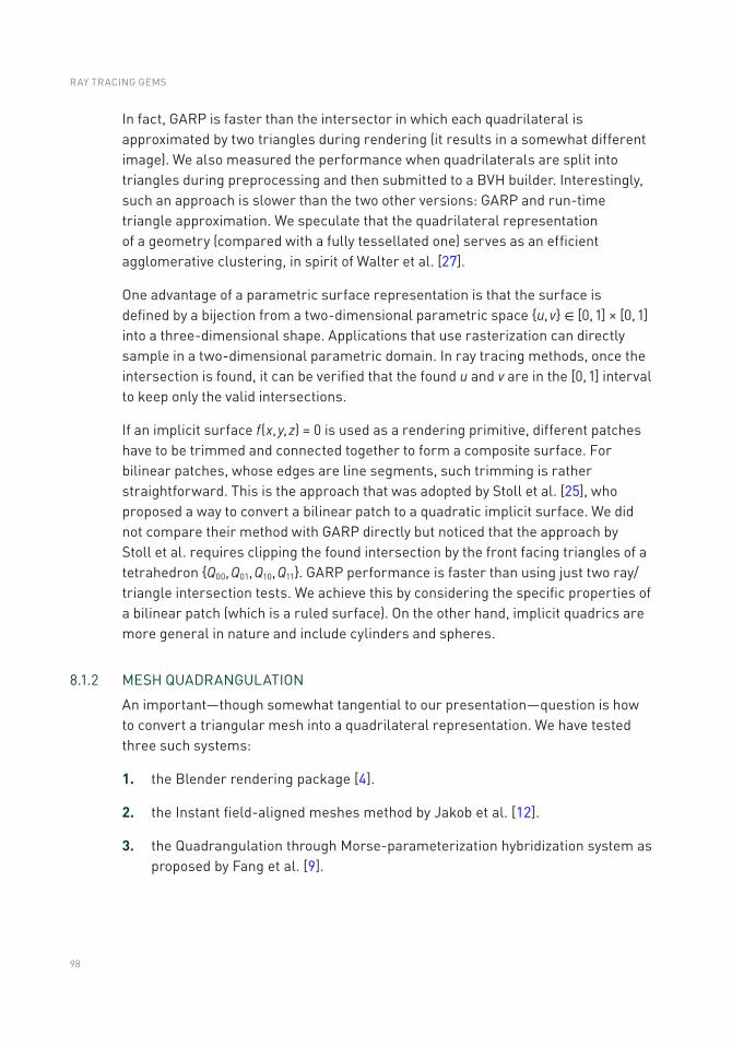
98
In fact, GARP is faster than the intersector in which each quadrilateral is approximated by two triangles during rendering (it results in a somewhat different image). We also measured the performance when quadrilaterals are split into triangles during preprocessing and then submitted to a BVH builder. Interestingly, such an approach is slower than the two other versions: GARP and run-time triangle approximation. We speculate that the quadrilateral representation of a geometry (compared with a fully tessellated one) serves as an efficient agglomerative clustering, in spirit of Walter et al. [27].
One advantage of a parametric surface representation is that the surface is defined by a bijection from a two-dimensional parametric space u, v ∈ [0, 1] × [0, 1] into a three- dimensional shape. Applications that use rasterization can directly sample in a two- dimensional parametric domain. In ray tracing methods, once the intersection is found, it can be verified that the found u and v are in the [0, 1] interval to keep only the valid intersections.
If an implicit surface f(x, y, z) = 0 is used as a rendering primitive, different patches have to be trimmed and connected together to form a composite surface. For bilinear patches, whose edges are line segments, such trimming is rather straightforward. This is the approach that was adopted by Stoll et al. [25], who proposed a way to convert a bilinear patch to a quadratic implicit surface. We did not compare their method with GARP directly but noticed that the approach by Stoll et al. requires clipping the found intersection by the front facing triangles of a tetrahedron Q00, Q01, Q10, Q11. GARP performance is faster than using just two ray/triangle intersection tests. We achieve this by considering the specific properties of a bilinear patch (which is a ruled surface). On the other hand, implicit quadrics are more general in nature and include cylinders and spheres.
8.1.2 MESH QUADRANGULATION
An important—though somewhat tangential to our presentation—question is how to convert a triangular mesh into a quadrilateral representation. We have tested three such systems:
1. the Blender rendering package [4].
2. the Instant field-aligned meshes method by Jakob et al. [12].
3. the Quadrangulation through Morse-parameterization hybridization system as proposed by Fang et al. [9].
RAY TRACING GEMS
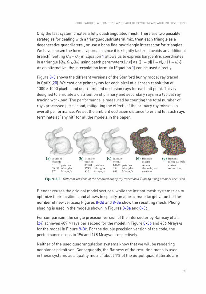
99
Only the last system creates a fully quadrangulated mesh. There are two possible strategies for dealing with a triangle/quadrilateral mix: treat each triangle as a degenerative quadrilateral, or use a bona fide ray/triangle intersector for triangles. We have chosen the former approach since it is slightly faster (it avoids an additional branch). Setting Q11 = Q10 in Equation 1 allows us to express barycentric coordinates in a triangle Q00, Q10, Q01 using patch parameters u, v as (1 − u)(1 − v), u, (1 − u)v. As an alternative, the interpolation formula (Equation 1) can be used directly.
Figure 8-3 shows the different versions of the Stanford bunny model ray traced in OptiX [20]. We cast one primary ray for each pixel at a screen resolution of 1000 × 1000 pixels, and use 9 ambient occlusion rays for each hit point. This is designed to emulate a distribution of primary and secondary rays in a typical ray tracing workload. The performance is measured by counting the total number of rays processed per second, mitigating the effects of the primary ray misses on overall performance. We set the ambient occlusion distance to ∞ and let such rays terminate at “any hit” for all the models in the paper.
Figure 8-3. Different versions of the Stanford bunny ray traced on a Titan Xp using ambient occlusion.
Blender reuses the original model vertices, while the instant mesh system tries to optimize their positions and allows to specify an approximate target value for the number of new vertices; Figures 8-3d and 8-3e show the resulting mesh. Phong shading is used in the models shown in Figures 8-3a and 8-3c.
For comparison, the single precision version of the intersector by Ramsey et al. [24] achieves 409 Mrays per second for the model in Figure 8-3b and 406 Mrays/s for the model in Figure 8-3c. For the double precision version of the code, the performance drops to 196 and 198 Mrays/s, respectively.
Neither of the used quadrangulation systems know that we will be rendering nonplanar primitives. Consequently, the flatness of the resulting mesh is used in these systems as a quality metric (about 1% of the output quadrilaterals are
COOL PATCHES: A GEOMETRIC APPROACH TO RAy/BILINEAR PATCH INTERSECTIONS
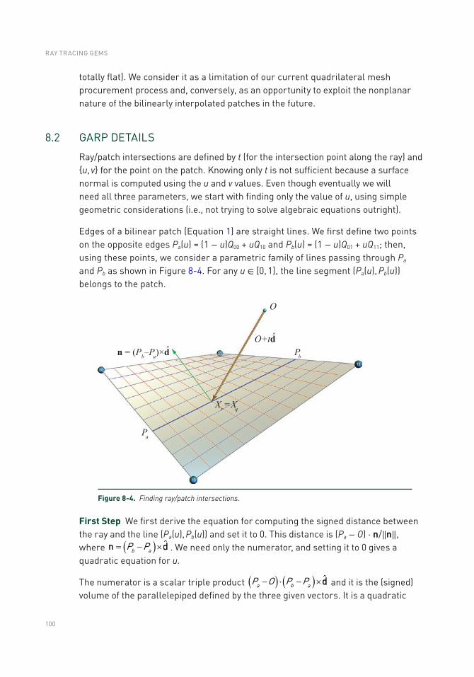
100
totally flat). We consider it as a limitation of our current quadrilateral mesh procurement process and, conversely, as an opportunity to exploit the nonplanar nature of the bilinearly interpolated patches in the future.
8.2 GARP DETAILS
Ray/patch intersections are defined by t (for the intersection point along the ray) and u, v for the point on the patch. Knowing only t is not sufficient because a surface normal is computed using the u and v values. Even though eventually we will need all three parameters, we start with finding only the value of u, using simple geometric considerations (i.e., not trying to solve algebraic equations outright).
Edges of a bilinear patch (Equation 1) are straight lines. We first define two points on the opposite edges Pa(u) = (1 − u)Q00 + uQ10 and Pb(u) = (1 − u)Q01 + uQ11; then, using these points, we consider a parametric family of lines passing through Pa and Pb as shown in Figure 8-4. For any u ∈ [0, 1], the line segment (Pa(u), Pb(u)) belongs to the patch.
Figure 8-4. Finding ray/patch intersections.
First Step We first derive the equation for computing the signed distance between the ray and the line (Pa(u), Pb(u)) and set it to 0. This distance is (Pa − O) ⋅ n/‖n‖, where ( )= - ´b aP P ˆn d . We need only the numerator, and setting it to 0 gives a quadratic equation for u.
The numerator is a scalar triple product ( ) ( ) ˆa b aP O P P- × - ´d and it is the (signed)
volume of the parallelepiped defined by the three given vectors. It is a quadratic
RAY TRACING GEMS
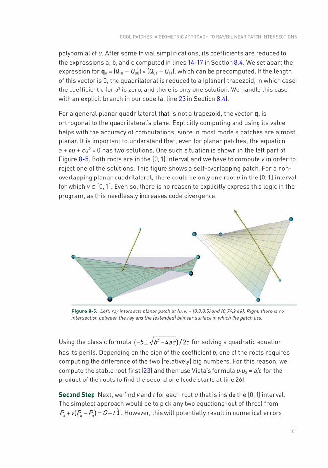
101
polynomial of u. After some trivial simplifications, its coefficients are reduced to the expressions a, b, and c computed in lines 14-17 in Section 8.4. We set apart the expression for qn = (Q10 − Q00) × (Q01 − Q11), which can be precomputed. If the length of this vector is 0, the quadrilateral is reduced to a (planar) trapezoid, in which case the coefficient c for u2 is zero, and there is only one solution. We handle this case with an explicit branch in our code (at line 23 in Section 8.4).
For a general planar quadrilateral that is not a trapezoid, the vector qn is orthogonal to the quadrilateral’s plane. Explicitly computing and using its value helps with the accuracy of computations, since in most models patches are almost planar. It is important to understand that, even for planar patches, the equation a + bu + cu2 = 0 has two solutions. One such situation is shown in the left part of Figure 8-5. Both roots are in the [0, 1] interval and we have to compute v in order to reject one of the solutions. This figure shows a self-overlapping patch. For a non-overlapping planar quadrilateral, there could be only one root u in the [0, 1] interval for which v ∈ [0, 1]. Even so, there is no reason to explicitly express this logic in the program, as this needlessly increases code divergence.
Figure 8-5. Left: ray intersects planar patch at u, v = 0.3,0.5 and 0.74,2.66. Right: there is no intersection between the ray and the (extended) bilinear surface in which the patch lies.
Using the classic formula - ± -( )b b ac c2 4 / 2 for solving a quadratic equation
has its perils. Depending on the sign of the coefficient b, one of the roots requires computing the difference of the two (relatively) big numbers. For this reason, we compute the stable root first [23] and then use Vieta’s formula u1u2 = a/c for the product of the roots to find the second one (code starts at line 26).
Second Step Next, we find v and t for each root u that is inside the [0, 1] interval. The simplest approach would be to pick any two equations (out of three) from
+ - = +( )a b aP v P P O t d . However, this will potentially result in numerical errors
COOL PATCHES: A GEOMETRIC APPROACH TO RAy/BILINEAR PATCH INTERSECTIONS
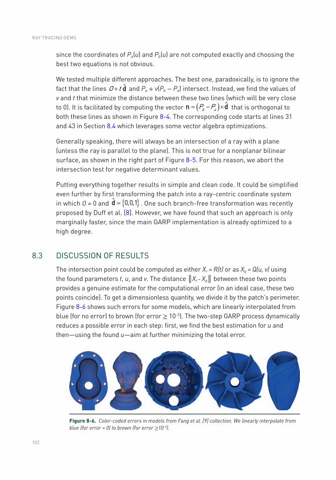
102
since the coordinates of Pa(u) and Pb(u) are not computed exactly and choosing the best two equations is not obvious.
We tested multiple different approaches. The best one, paradoxically, is to ignore the fact that the lines +O t d and Pa + v(Pb − Pa) intersect. Instead, we find the values of v and t that minimize the distance between these two lines (which will be very close to 0). It is facilitated by computing the vector ( )= - ´b aP P ˆn d that is orthogonal to both these lines as shown in Figure 8-4. The corresponding code starts at lines 31 and 43 in Section 8.4 which leverages some vector algebra optimizations.
Generally speaking, there will always be an intersection of a ray with a plane (unless the ray is parallel to the plane). This is not true for a nonplanar bilinear surface, as shown in the right part of Figure 8-5. For this reason, we abort the intersection test for negative determinant values.
Putting everything together results in simple and clean code. It could be simplified even further by first transforming the patch into a ray-centric coordinate system in which O = 0 and =ˆ 0,0,1d . One such branch-free transformation was recently proposed by Duff et al. [8]. However, we have found that such an approach is only marginally faster, since the main GARP implementation is already optimized to a high degree.
8.3 DISCUSSION OF RESULTS
The intersection point could be computed as either Xr = R(t) or as Xq = Q(u, v) using the found parameters t, u, and v. The distance Xr - Xq between these two points provides a genuine estimate for the computational error (in an ideal case, these two points coincide). To get a dimensionless quantity, we divide it by the patch’s perimeter. Figure 8-6 shows such errors for some models, which are linearly interpolated from blue (for no error) to brown (for error ≥ 10–5). The two-step GARP process dynamically reduces a possible error in each step: first, we find the best estimation for u and then—using the found u—aim at further minimizing the total error.
Figure 8-6. Color-coded errors in models from Fang et al. [9] collection. We linearly interpolate from blue (for error = 0) to brown (for error ≥10−5).
RAY TRACING GEMS
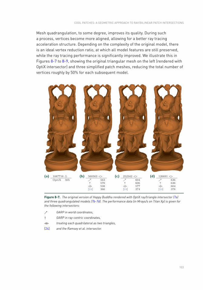
103
Figure 8-7. The original version of Happy Buddha rendered with OptiX ray/triangle intersector (7a) and three quadrangulated models (7b-7d). The performance data (in Mrays/s on Titan Xp) is given for the following intersectors:
GARP in world coordinates,
↑ GARP in ray-centric coordinates,
⊲⊳ treating each quadrilateral as two triangles,
[24] and the Ramsey et al. intersector.
Mesh quadrangulation, to some degree, improves its quality. During such a process, vertices become more aligned, allowing for a better ray tracing acceleration structure. Depending on the complexity of the original model, there is an ideal vertex reduction ratio, at which all model features are still preserved, while the ray tracing performance is significantly improved. We illustrate this in Figures 8-7 to 8-9, showing the original triangular mesh on the left (rendered with OptiX intersector) and three simplified patch meshes, reducing the total number of vertices roughly by 50% for each subsequent model.
COOL PATCHES: A GEOMETRIC APPROACH TO RAy/BILINEAR PATCH INTERSECTIONS
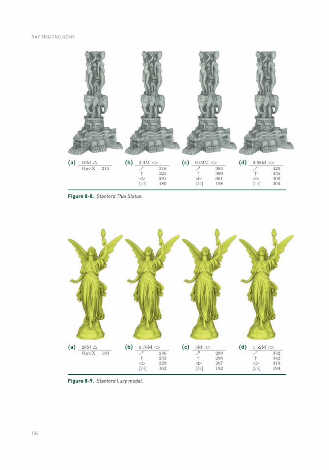
104
Figure 8-8. Stanford Thai Statue.
Figure 8-9. Stanford Lucy model.
RAY TRACING GEMS
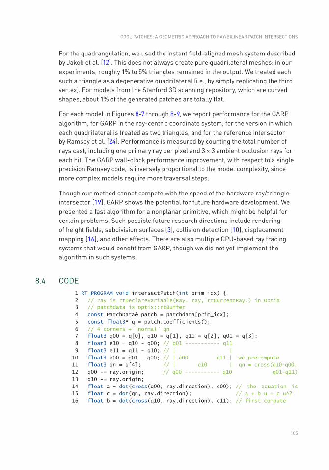
105
For the quadrangulation, we used the instant field-aligned mesh system described by Jakob et al. [12]. This does not always create pure quadrilateral meshes: in our experiments, roughly 1% to 5% triangles remained in the output. We treated each such a triangle as a degenerative quadrilateral (i.e., by simply replicating the third vertex). For models from the Stanford 3D scanning repository, which are curved shapes, about 1% of the generated patches are totally flat.
For each model in Figures 8-7 through 8-9, we report performance for the GARP algorithm, for GARP in the ray-centric coordinate system, for the version in which each quadrilateral is treated as two triangles, and for the reference intersector by Ramsey et al. [24]. Performance is measured by counting the total number of rays cast, including one primary ray per pixel and 3 × 3 ambient occlusion rays for each hit. The GARP wall-clock performance improvement, with respect to a single precision Ramsey code, is inversely proportional to the model complexity, since more complex models require more traversal steps.
Though our method cannot compete with the speed of the hardware ray/triangle intersector [19], GARP shows the potential for future hardware development. We presented a fast algorithm for a nonplanar primitive, which might be helpful for certain problems. Such possible future research directions include rendering of height fields, subdivision surfaces [3], collision detection [10], displacement mapping [16], and other effects. There are also multiple CPU-based ray tracing systems that would benefit from GARP, though we did not yet implement the algorithm in such systems.
8.4 CODE 1 RT_PROGRAM void intersectPatch(int prim_idx)
2 // ray is rtDeclareVariable(Ray, ray, rtCurrentRay,) in OptiX
3 // patchdata is optix::rtBuffer
4 const PatchData& patch = patchdata[prim_idx];
5 const float3* q = patch.coefficients();
6 // 4 corners + "normal" qn
7 float3 q00 = q[0], q10 = q[1], q11 = q[2], q01 = q[3];
8 float3 e10 = q10 - q00; // q01 ----------- q11
9 float3 e11 = q11 - q10; // | |
10 float3 e00 = q01 - q00; // | e00 e11 | we precompute
11 float3 qn = q[4]; // | e10 | qn = cross(q10-q00,
12 q00 -= ray.origin; // q00 ----------- q10 q01-q11)
13 q10 -= ray.origin;
14 float a = dot(cross(q00, ray.direction), e00); // the equation is
15 float c = dot(qn, ray.direction); // a + b u + c u^2
16 float b = dot(cross(q10, ray.direction), e11); // first compute
COOL PATCHES: A GEOMETRIC APPROACH TO RAy/BILINEAR PATCH INTERSECTIONS
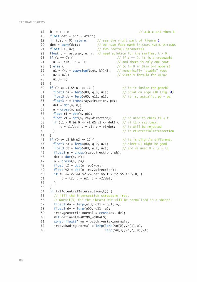
106
17 b -= a + c; // a+b+c and then b
18 float det = b*b - 4*a*c;
19 if (det < 0) return; // see the right part of Figure 5
20 det = sqrt(det); // we -use_fast_math in CUDA_NVRTC_OPTIONS
21 float u1, u2; // two roots(u parameter)
22 float t = ray.tmax, u, v; // need solution for the smallest t > 0
23 if (c == 0) // if c == 0, it is a trapezoid
24 u1 = -a/b; u2 = -1; // and there is only one root
25 else // (c != 0 in Stanford models)
26 u1 = (-b - copysignf(det, b))/2; // numerically "stable" root
27 u2 = a/u1; // Viete's formula for u1*u2
28 u1 /= c;
29
30 if (0 <= u1 && u1 <= 1) // is it inside the patch?
31 float3 pa = lerp(q00, q10, u1); // point on edge e10 (Fig. 4)
32 float3 pb = lerp(e00, e11, u1); // it is, actually, pb - pa
33 float3 n = cross(ray.direction, pb);
34 det = dot(n, n);
35 n = cross(n, pa);
36 float t1 = dot(n, pb);
37 float v1 = dot(n, ray.direction); // no need to check t1 < t
38 if (t1 > 0 && 0 <= v1 && v1 <= det) // if t1 > ray.tmax,
39 t = t1/det; u = u1; v = v1/det; // it will be rejected
40 // in rtPotentialIntersection
41
42 if (0 <= u2 && u2 <= 1) // it is slightly different,
43 float3 pa = lerp(q00, q10, u2); // since u1 might be good
44 float3 pb = lerp(e00, e11, u2); // and we need 0 < t2 < t1
45 float3 n = cross(ray.direction, pb);
46 det = dot(n, n);
47 n = cross(n, pa);
48 float t2 = dot(n, pb)/det;
49 float v2 = dot(n, ray.direction);
50 if (0 <= v2 && v2 <= det && t > t2 && t2 > 0)
51 t = t2; u = u2; v = v2/det;
52
53
54 if (rtPotentialIntersection(t))
55 // Fill the intersection structure irec.
56 // Normal(s) for the closest hit will be normalized in a shader.
57 float3 du = lerp(e10, q11 - q01, v);
58 float3 dv = lerp(e00, e11, u);
59 irec.geometric_normal = cross(du, dv);
60 #if defined(SHADING_NORMALS)
61 const float3* vn = patch.vertex_normals;
62 irec.shading_normal = lerp(lerp(vn[0],vn[1],u),
63 lerp(vn[3],vn[2],u),v);
RAY TRACING GEMS
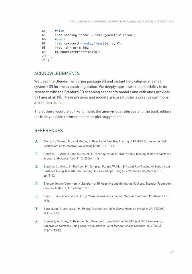
107
64 #else
65 irec.shading_normal = irec.geometric_normal;
66 #endif
67 irec.texcoord = make_float3(u, v, 0);
68 irec.id = prim_idx;
69 rtReportIntersection(0u);
70
71
ACKNOWLEDGMENTS
We used the Blender rendering package [4] and instant field-aligned meshes system [12] for mesh quadrangulation. We deeply appreciate the possibility to do research with the Stanford 3D scanning repository models and with ones provided by Fang at al. [9]. These systems and models are used under a creative commons attribution license.
The authors would also like to thank the anonymous referees and the book editors for their valuable comments and helpful suggestions.
REFERENCES
[1] Abert, O., Geimer, M., and Muller, S. Direct and Fast Ray Tracing of NURBS Surfaces. In IEEE Symposium on Interactive Ray Tracing (2006), 161–168.
[2] Benthin, C., Wald, I., and Slusallek, P. Techniques for Interactive Ray Tracing of Bézier Surfaces. Journal of Graphics Tools 11, 2 (2006), 1–16.
[3] Benthin, C., Woop, S., Nießner, M., Selgrad, K., and Wald, I. Efficient Ray Tracing of Subdivision Surfaces Using Tessellation Caching. In Proceedings of High- Performance Graphics (2015), pp. 5–12.
[4] Blender Online Community. Blender—a 3D Modelling and Rendering Package. Blender Foundation, Blender Institute, Amsterdam, 2018.
[5] Blinn, J. Jim Blinn’s Corner: A Trip Down the Graphics Pipeline. Morgan Kaufmann Publishers Inc., 1996.
[6] Boubekeur, T., and Alexa, M. Phong Tessellation. ACM Transactions on Graphics 27, 5 (2008), 141:1–141:5.
[7] Brainerd, W., Foley, T., Kraemer, M., Moreton, H., and Nießner, M. Efficient GPU Rendering of Subdivision Surfaces Using Adaptive Quadtrees. ACM Transactions on Graphics 35, 4 (2016), 113:1–113:12.
COOL PATCHES: A GEOMETRIC APPROACH TO RAy/BILINEAR PATCH INTERSECTIONS

108
[8] Duff, T., Burgess, J., Christensen, P., Hery, C., Kensler, A., Liani, M., and Villemin, R. Building an Orthonormal Basis, Revisited. Journal of Computer Graphics Techniques 6, 1 (March 2017), 1–8.
[9] Fang, X., Bao, H., Tong, y., Desbrun, M., and Huang, J. Quadrangulation Through Morse-Parameterization Hybridization. ACM Transactions on Graphics 37, 4 (2018), 92:1–92:15.
[10] Fournier, A., and Buchanan, J. Chebyshev Polynomials for Boxing and Intersections of Parametric Curves and Surfaces. Computer Graphics Forum 13, 3 (1994), 127–142.
[11] Hanrahan, P. Ray-Triangle and Ray-Quadrilateral Intersections in Homogeneous Coordinates, http://graphics.stanford.edu/courses/cs348b-04/rayhomo.pdf, 1989.
[12] Jakob, W., Tarini, M., Panozzo, D., and Sorkine-Hornung, O. Instant Field-Aligned Meshes. ACM Transactions on Graphics 34, 6 (Nov. 2015), 189:1–189:15.
[13] Kajiya, J. T. Ray Tracing Parametric Patches. Computer Graphics (SIGGRAPH) 16, 3 (July 1982), 245–254.
[14] Kensler, A., and Shirley, P. Optimizing Ray-Triangle Intersection via Automated Search. IEEE Symposium on Interactive Ray Tracing (2006), 33–38.
[15] Lagae, A., and Dutré, P. An Efficient Ray-Quadrilateral Intersection Test. Journal of Graphics Tools 10, 4 (2005), 23–32.
[16] Lier, A., Martinek, M., Stamminger, M., and Selgrad, K. A High-Resolution Compression Scheme for Ray Tracing Subdivision Surfaces with Displacement. Proceedings of the ACM on Computer Graphics and Interactive Techniques 1, 2 (2018), 33:1–33:17.
[17] Loop, C., Schaefer, S., Ni, T., and Castaño, I. Approximating Subdivision Surfaces with Gregory Patches for Hardware Tessellation. ACM Transactions on Graphics 28, 5 (2009), 151:1–151:9.
[18] Mao, Z., Ma, L., and Zhao, M. G1 Continuity Triangular Patches Interpolation Based on PN Triangles. In International Conference on Computational Science (2005), pp. 846–849.
[19] NVIDIA. NVIDIA RTX™ platform, https://developer.nvidia.com/rtx, 2018.
[20] Parker, S. G., Bigler, J., Dietrich, A., Friedrich, H., Hoberock, J., Luebke, D., McAllister, D., McGuire, M., Morley, K., Robison, A., and Stich, M. OptiX: A General Purpose Ray Tracing Engine. ACM Transactions on Graphics 29, 4 (2010), 66:1–66:13.
[21] Peters, J. Smooth Free-Form Surfaces over Irregular Meshes Generalizing Quadratic Splines. In International Symposium on Free-form Curves and Free-form Surfaces (1993), pp. 347–361.
[22] Phong, B. T. Illumination for Computer-Generated Images. PhD thesis, The University of Utah, 1973.
[23] Press, W. H., Teukolsky, S. A., Vetterling, W. T., and Flannery, B. P. Numerical Recipes 3rd Edition: The Art of Scientific Computing, 3 ed. Cambridge University Press, 2007.
[24] Ramsey, S. D., Potter, K., and Hansen, C. D. Ray Bilinear Patch Intersections. Journal of Graphics, GPU, & Game Tools 9, 3 (2004), 41–47.
RAY TRACING GEMS

109
[25] Stoll, C., Gumhold, S., and Seidel, H.-P. Incremental Raycasting of Piecewise Quadratic Surfaces on the GPU. In IEEE Symposium on Interactive Ray Tracing (2006), pp. 141–150.
[26] Vlachos, A., Peters, J., Boyd, C., and Mitchell, J. L. Curved PN Triangles. In Symposium on Interactive 3D Graphics (2001), pp. 159–166.
[27] Walter, B., Bala, K., Kulkarni, M. N., and Pingali, K. Fast Agglomerative Clustering for Rendering. IEEE Symposium on Interactive Ray Tracing (2008), 81–86.
[28] Wong, S., and Cendes, Z. C1 Quadratic Interpolation over Arbitrary Point Sets. IEEE Computer Graphics and Applications 7, 11 (1987), 8–16.
Open Access This chapter is licensed under the terms of the Creative Commons Attribution-NonCommercial-NoDerivatives 4.0 International License (http://creativecommons.org/licenses/by-nc-nd/4.0/), which permits any noncommercial use, sharing, distribution and
reproduction in any medium or format, as long as you give appropriate credit to the original author(s) and the source, provide a link to the Creative Commons license and indicate if you modified the licensed material. you do not have permission under this license to share adapted material derived from this chapter or parts of it.
The images or other third party material in this chapter are included in the chapter's Creative Commons license, unless indicated otherwise in a credit line to the material. If material is not included in the chapter's Creative Commons license and your intended use is not permitted by statutory regulation or exceeds the permitted use, you will need to obtain permission directly from the copyright holder.
COOL PATCHES: A GEOMETRIC APPROACH TO RAy/BILINEAR PATCH INTERSECTIONS
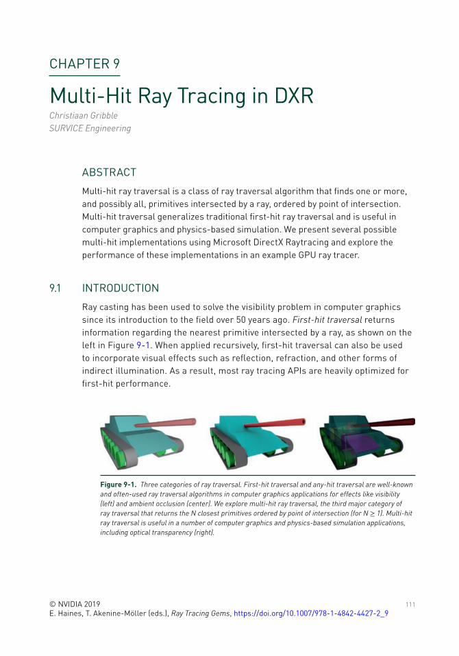
111© NVIDIA 2019 E. Haines, T. Akenine-Möller (eds.), Ray Tracing Gems, https://doi.org/10.1007/978-1-4842-4427-2_9
CHAPTER 9
Multi-Hit Ray Tracing in DXRChristiaan Gribble SURVICE Engineering
ABSTRACT
Multi-hit ray traversal is a class of ray traversal algorithm that finds one or more, and possibly all, primitives intersected by a ray, ordered by point of intersection. Multi- hit traversal generalizes traditional first-hit ray traversal and is useful in computer graphics and physics-based simulation. We present several possible multi-hit implementations using Microsoft DirectX Raytracing and explore the performance of these implementations in an example GPU ray tracer.
9.1 INTRODUCTION
Ray casting has been used to solve the visibility problem in computer graphics since its introduction to the field over 50 years ago. First-hit traversal returns information regarding the nearest primitive intersected by a ray, as shown on the left in Figure 9-1. When applied recursively, first-hit traversal can also be used to incorporate visual effects such as reflection, refraction, and other forms of indirect illumination. As a result, most ray tracing APIs are heavily optimized for first-hit performance.
Figure 9-1. Three categories of ray traversal. First-hit traversal and any-hit traversal are well-known and often-used ray traversal algorithms in computer graphics applications for effects like visibility (left) and ambient occlusion (center). We explore multi-hit ray traversal, the third major category of ray traversal that returns the N closest primitives ordered by point of intersection (for N ≥ 1). Multi- hit ray traversal is useful in a number of computer graphics and physics-based simulation applications, including optical transparency (right).
112
A second class of ray traversal, any-hit traversal, also finds application in computer graphics. With any-hit traversal, the intersection query is not constrained to return the nearest primitive but simply whether or not a ray intersects any primitive within a specified interval. Any-hit traversal is particularly useful for effects such as shadows and ambient occlusion, as shown in the center in Figure 9-1.
In the third class of traversal, multi-hit ray traversal [5], an intersection query returns information concerning the N closest primitives intersected by a ray. Multi-hit traversal generalizes both first-hit traversal (where N = 1) and all-hit traversal, a scheme in which ray queries return information concerning every intersected primitive (where N = ∞), while accommodating arbitrary values of N between these extremes.
Multi-hit traversal is useful in a number of computer graphics applications, for example, fast and accurate rendering of transparent objects. Raster-based solutions impose expensive fragment sorting on the GPU and must be extended to render coplanar objects correctly.1 In contrast, multi-hit traversal offers a straightforward means to implement high-performance transparent rendering while handling overlapping coplanar objects correctly.
Importantly, multi-hit traversal can also be used in a wide variety of physics-based simulations, or so-called non-optical rendering, as shown on the right in Figure 9-1. In domains such as ballistic penetration, radio frequency propagation, and thermal radiative transport, among others, the relevant phenomena are governed by equations similar to the Beer-Lambert Law and so require ray/primitive intervals, not just intersection points. These simulations are similar to rendering scenes in which all objects behave as participating media.
A correct multi-hit ray traversal algorithm is a necessary, but insufficient, condition for modern applications; performance is also critical for both interactivity and fidelity in many scenarios. Modern ray tracing engines address performance concerns by hiding complicated, highly optimized ray tracing kernels behind clean, well-designed APIs. To accelerate ray queries, these engines use numerous bounding volume hierarchy (BVH) variants based on application characteristics provided to the engine by the user. These engines provide fast first-hit and any-hit ray traversal operations for use in applications across optical and non-optical domains, but they do not typically support multi-hit ray traversal as a fundamental operation.
1 The problem of coplanar objects, both in transparent rendering and in physics-based simulation, is discussed more thoroughly by, for example, Gribble et al. [5]; interested readers are referred to the literature for additional details.
RAY TRACING GEMS
113
Early work on multi-hit ray traversal [5] assumes an acceleration structure based on spatial subdivision, in which leaf nodes of the structure do not overlap. With such structures, ordered traversal—and therefore generating ordered hit points—is straightforward: sorting is required only within, not across, leaf nodes. However, ordered traversal in a structure based on object partitioning, such as a BVH, is not achieved so easily. While an implementation based on a traversal priority queue (rather than a traversal stack) enables front-to-back traversal of a BVH [7], most publicly available, widely used production ray tracing APIs do not provide ordered BVH traversal variants.
However, these APIs, including Microsoft DirectX Raytracing (DXR), expose features enabling implementation of multi-hit ray tracing entirely with user-level code, thereby leveraging their existing—and heavily optimized—BVH construction and traversal routines. In the remainder of this chapter, we present several possible multi- hit implementations using DXR and explore their performance in an example GPU ray tracing application. Source and binary distributions of this application are available [4], permitting readers to explore, modify, or enhance these DXR multi-hit implementations.
9.2 IMPLEMENTATION
As noted in Section 9.1 and discussed in detail by Amstutz et al. [1], the problem of multi- hit ray tracing with unordered BVH traversal variants is compounded by overlapping nodes. Correctness requires either naive multi-hit traversal [5], which is potentially slow, or modification of BVH construction or traversal routines, which not only imposes potentially significant development and maintenance burdens in production environments, but is simply not possible with implementation-neutral ray tracing APIs.
To address these issues, we present two DXR implementations each of two multi-hit traversal algorithms: naive multi-hit traversal and node-culling multi-hit BVH traversal [3]. Our first implementation of each algorithm leverages DXR any-hit shaders to satisfy multi-hit intersection queries along each ray. DXR any-hit shaders execute whenever a ray intersects a geometry instance within the current ray interval, [tmin, tmax], regardless of its position along the ray relative to other intersections. These shaders do not follow any defined order of execution for intersections along a ray. If an any-hit shader accepts a potential intersection, its hit distance becomes the new maximum value for the ray interval, tmax.
Our second implementation of each algorithm satisfies multi-hit queries using DXR intersection shaders, which offer an alternative representation for geometry in a bottom- level acceleration structure. In this case, the procedural primitive is
MULTI-HIT RAy TRACING IN DXR
114
defined by its axis-aligned bounding box, and a user-defined intersection shader evaluates primitive intersections when a ray intersects that box. The intersection shader defines attributes describing intersections, including the current hit distance, that are then passed to subsequent shaders. Generally speaking, DXR intersection shaders are less efficient than the built-in ray/triangle intersection routines, but they offer far more flexibility. We exploit these shaders to implement both naive and node-culling multi-hit ray traversal for triangle primitives as an alternative to the DXR any-hit shader implementations.
In these implementations, each shader assumes buffers for storing multi-hit results: a two-dimensional (width × height) buffer for per-ray hit counts and a three-dimensional (width × height × (Nquery + 1)) buffer for hit records, each comprising a hit-point intersection distance (t-value), the diffuse surface color, and the value Ng ⋅ V to support simple surface shading operations. The any-hit shader implementations use a user- defined ray payload structure to track the current number of hits and require setting the D3D12_RAYTRACING_GEOMETRY_FLAG_NO_DUPLICATE_ANYHIT_INVOCATION geometry flag to disallow multiple any-hit shader invocations. The corresponding ray generation shaders set the RAY_FLAG_FORCE_NON_OPAQUE ray flag to treat all ray/primitive intersections as non-opaque. In contrast, the intersection shader implementations require buffers storing triangle vertices, faces, and material data, properties typically managed by DXR when using the built-in triangle primitives.
All shaders rely on utility functions for shader-side buffer management, color mapping for visualization, and so forth. Likewise, each shader assumes values controlling the final rendered results, including Nquery, background color, and various color-mapping parameters affecting the visualization modes supported by our example application. Other DXR shader states and parameters—for example, the two- dimensional output buffer storing rendered results—are ultimately managed by Falcor [2], the real-time rendering framework underlying our application. For clarity and focus of presentation, these elements are omitted from the implementation highlights that follow.
Our example ray tracing application leverages Chris Wyman’s dxrTutors.Code project [8], which itself builds on Falcor, to manage DXR states. The project dxrTutors.Code provides a highly abstracted CPU-side C++ DXR API, designed both to aid programmers in getting DXR applications running quickly and to enable easy experimentation. While these dependencies are required to build our multi-hit ray tracing application from source, the multi-hit DXR shaders themselves can be adapted to other frameworks that provide similar DXR abstractions in a straightforward manner. We highlight these implementations in the remainder of this section, and we explore the resulting performance in Section 9.3.
RAY TRACING GEMS
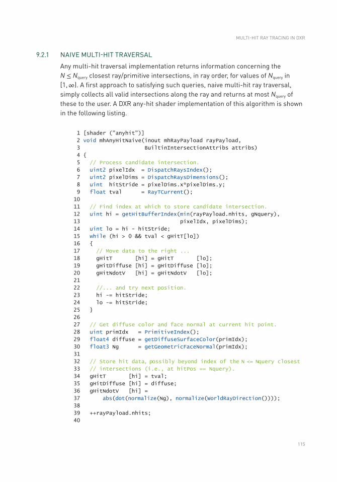
115
9.2.1 NAIVE MULTI-HIT TRAVERSAL
Any multi-hit traversal implementation returns information concerning the N ≤ Nquery closest ray/primitive intersections, in ray order, for values of Nquery in [1, ∞). A first approach to satisfying such queries, naive multi-hit ray traversal, simply collects all valid intersections along the ray and returns at most Nquery of these to the user. A DXR any-hit shader implementation of this algorithm is shown in the following listing.
1 [shader ("anyhit")]
2 void mhAnyHitNaive(inout mhRayPayload rayPayload,
3 BuiltinIntersectionAttribs attribs)
4
5 // Process candidate intersection.
6 uint2 pixelIdx = DispatchRaysIndex();
7 uint2 pixelDims = DispatchRaysDimensions();
8 uint hitStride = pixelDims.x*pixelDims.y;
9 float tval = RayTCurrent();
10
11 // Find index at which to store candidate intersection.
12 uint hi = getHitBufferIndex(min(rayPayload.nhits, gNquery),
13 pixelIdx, pixelDims);
14 uint lo = hi - hitStride;
15 while (hi > 0 && tval < gHitT[lo])
16
17 // Move data to the right ...
18 gHitT [hi] = gHitT [lo];
19 gHitDiffuse [hi] = gHitDiffuse [lo];
20 gHitNdotV [hi] = gHitNdotV [lo];
21
22 //... and try next position.
23 hi -= hitStride;
24 lo -= hitStride;
25
26
27 // Get diffuse color and face normal at current hit point.
28 uint primIdx = PrimitiveIndex();
29 float4 diffuse = getDiffuseSurfaceColor(primIdx);
30 float3 Ng = getGeometricFaceNormal(primIdx);
31
32 // Store hit data, possibly beyond index of the N <= Nquery closest
33 // intersections (i.e., at hitPos == Nquery).
34 gHitT [hi] = tval;
35 gHitDiffuse [hi] = diffuse;
36 gHitNdotV [hi] =
37 abs(dot(normalize(Ng), normalize(WorldRayDirection())));
38
39 ++rayPayload.nhits;
40
MULTI-HIT RAy TRACING IN DXR
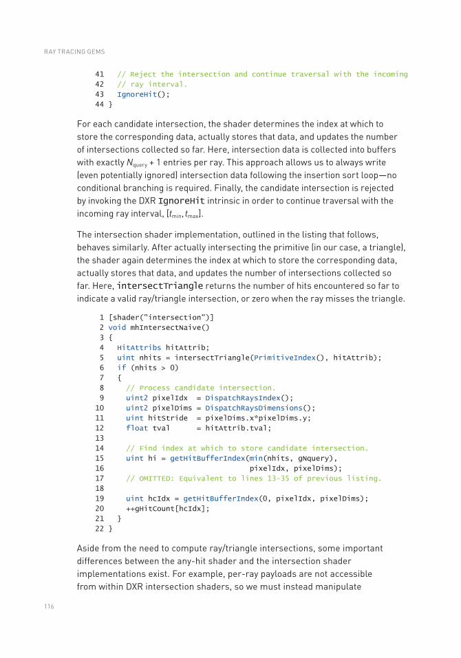
116
41 // Reject the intersection and continue traversal with the incoming
42 // ray interval.
43 IgnoreHit();
44
For each candidate intersection, the shader determines the index at which to store the corresponding data, actually stores that data, and updates the number of intersections collected so far. Here, intersection data is collected into buffers with exactly Nquery + 1 entries per ray. This approach allows us to always write (even potentially ignored) intersection data following the insertion sort loop—no conditional branching is required. Finally, the candidate intersection is rejected by invoking the DXR IgnoreHit intrinsic in order to continue traversal with the incoming ray interval, [tmin, tmax].
The intersection shader implementation, outlined in the listing that follows, behaves similarly. After actually intersecting the primitive (in our case, a triangle), the shader again determines the index at which to store the corresponding data, actually stores that data, and updates the number of intersections collected so far. Here, intersectTriangle returns the number of hits encountered so far to indicate a valid ray/triangle intersection, or zero when the ray misses the triangle.
1 [shader("intersection")]
2 void mhIntersectNaive()
3
4 HitAttribs hitAttrib;
5 uint nhits = intersectTriangle(PrimitiveIndex(), hitAttrib);
6 if (nhits > 0)
7
8 // Process candidate intersection.
9 uint2 pixelIdx = DispatchRaysIndex();
10 uint2 pixelDims = DispatchRaysDimensions();
11 uint hitStride = pixelDims.x*pixelDims.y;
12 float tval = hitAttrib.tval;
13
14 // Find index at which to store candidate intersection.
15 uint hi = getHitBufferIndex(min(nhits, gNquery),
16 pixelIdx, pixelDims);
17 // OMITTED: Equivalent to lines 13-35 of previous listing.
18
19 uint hcIdx = getHitBufferIndex(0, pixelIdx, pixelDims);
20 ++gHitCount[hcIdx];
21
22
Aside from the need to compute ray/triangle intersections, some important differences between the any-hit shader and the intersection shader implementations exist. For example, per-ray payloads are not accessible from within DXR intersection shaders, so we must instead manipulate
RAY TRACING GEMS
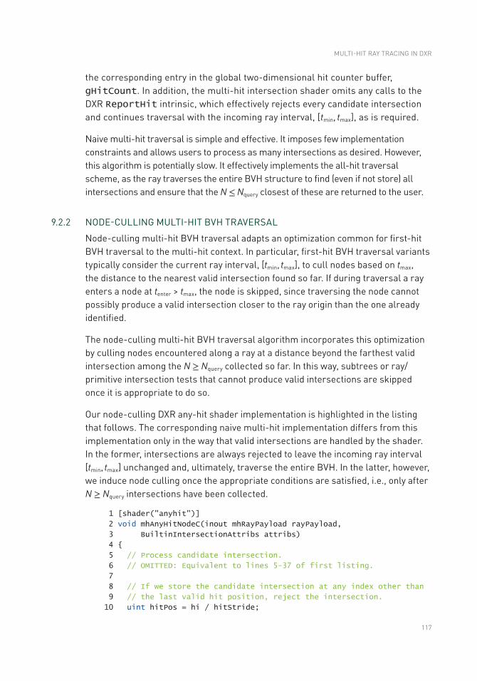
117
the corresponding entry in the global two- dimensional hit counter buffer, gHitCount. In addition, the multi-hit intersection shader omits any calls to the DXR ReportHit intrinsic, which effectively rejects every candidate intersection and continues traversal with the incoming ray interval, [tmin, tmax], as is required.
Naive multi-hit traversal is simple and effective. It imposes few implementation constraints and allows users to process as many intersections as desired. However, this algorithm is potentially slow. It effectively implements the all-hit traversal scheme, as the ray traverses the entire BVH structure to find (even if not store) all intersections and ensure that the N ≤ Nquery closest of these are returned to the user.
9.2.2 NODE-CULLING MULTI-HIT BVH TRAVERSAL
Node-culling multi-hit BVH traversal adapts an optimization common for first-hit BVH traversal to the multi-hit context. In particular, first-hit BVH traversal variants typically consider the current ray interval, [tmin, tmax], to cull nodes based on tmax, the distance to the nearest valid intersection found so far. If during traversal a ray enters a node at tenter > tmax, the node is skipped, since traversing the node cannot possibly produce a valid intersection closer to the ray origin than the one already identified.
The node-culling multi-hit BVH traversal algorithm incorporates this optimization by culling nodes encountered along a ray at a distance beyond the farthest valid intersection among the N ≥ Nquery collected so far. In this way, subtrees or ray/primitive intersection tests that cannot produce valid intersections are skipped once it is appropriate to do so.
Our node-culling DXR any-hit shader implementation is highlighted in the listing that follows. The corresponding naive multi-hit implementation differs from this implementation only in the way that valid intersections are handled by the shader. In the former, intersections are always rejected to leave the incoming ray interval [tmin, tmax] unchanged and, ultimately, traverse the entire BVH. In the latter, however, we induce node culling once the appropriate conditions are satisfied, i.e., only after N ≥ Nquery intersections have been collected.
1 [shader("anyhit")]
2 void mhAnyHitNodeC(inout mhRayPayload rayPayload,
3 BuiltinIntersectionAttribs attribs)
4
5 // Process candidate intersection.
6 // OMITTED: Equivalent to lines 5-37 of first listing.
7
8 // If we store the candidate intersection at any index other than
9 // the last valid hit position, reject the intersection.
10 uint hitPos = hi / hitStride;
MULTI-HIT RAy TRACING IN DXR
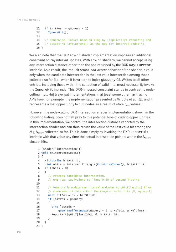
118
11 if (hitPos != gNquery - 1)
12 IgnoreHit();
13
14 // Otherwise, induce node culling by (implicitly) returning and
15 // accepting RayTCurrent() as the new ray interval endpoint.
16
We also note that the DXR any-hit shader implementation imposes an additional constraint on ray interval updates: With any-hit shaders, we cannot accept using any intersection distance other than the one returned by the DXR RayTCurrent intrinsic. As a result, the implicit return-and-accept behavior of the shader is valid only when the candidate intersection is the last valid intersection among those collected so far (i.e., when it is written to index gNquery-1). Writes to all other entries, including those within the collection of valid hits, must necessarily invoke the IgnoreHit intrinsic. This DXR-imposed constraint stands in contrast to node-culling multi-hit traversal implementations in at least some other ray tracing APIs (see, for example, the implementation presented by Gribble et al. [6]), and it represents a lost opportunity to cull nodes as a result of stale tmax values.
However, the node-culling DXR intersection shader implementation, shown in the following listing, does not fall prey to this potential loss of culling opportunities. In this implementation, we control the intersection distance reported by the intersection shader and can thus return the value of the last valid hit among the N ≥ Nquery collected so far. This is done simply by invoking the DXR ReportHit intrinsic with that value any time the actual intersection point is within the Nquery closest hits.
1 [shader("intersection")]
2 void mhIntersectNodeC()
3
4 HitAttribs hitAttrib;
5 uint nhits = intersectTriangle(PrimitiveIndex(), hitAttrib);
6 if (nhits > 0)
7
8 // Process candidate intersection.
9 // OMITTED: Equivalent to lines 9-20 of second listing.
10
11 // Potentially update ray interval endpoint to gHitT[lastIdx] if we
12 // wrote new hit data within the range of valid hits [0, Nquery-1].
13 uint hitPos = hi / hitStride;
14 if (hitPos < gNquery)
15
16 uint lastIdx =
17 getHitBufferIndex(gNquery - 1, pixelIdx, pixelDims);
18 ReportHit(gHitT[lastIdx], 0, hitAttrib);
19
20
21
RAY TRACING GEMS
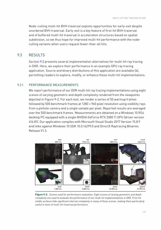
119
Node-culling multi-hit BVH traversal exploits opportunities for early-exit despite unordered BVH traversal. Early-exit is a key feature of first-hit BVH traversal and of buffered multi-hit traversal in acceleration structures based on spatial subdivision, so we thus hope for improved multi-hit performance with the node-culling variants when users request fewer-than-all hits.
9.3 RESULTS
Section 9.2 presents several implementation alternatives for multi-hit ray tracing in DXR. Here, we explore their performance in an example GPU ray tracing application. Source and binary distributions of this application are available [4], permitting readers to explore, modify, or enhance these multi-hit implementations.
9.3.1 PERFORMANCE MEASUREMENTS
We report performance of our DXR multi-hit ray tracing implementations using eight scenes of varying geometric and depth complexity rendered from the viewpoints depicted in Figure 9-2. For each test, we render a series of 50 warmup frames followed by 500 benchmark frames at 1280 × 960 pixel resolution using visibility rays from a pinhole camera and a single sample per pixel. Reported results are averaged over the 500 benchmark frames. Measurements are obtained on a Windows 10 RS4 desktop PC equipped with a single NVIDIA GeForce RTX 2080 Ti GPU (driver version 416.81). Our application compiles with Microsoft Visual Studio 2017 Version 15.8.9 and links against Windows 10 SDK 10.0.16299.0 and DirectX Raytracing Binaries Release V1.3.
Figure 9-2. Scenes used for performance evaluation. Eight scenes of varying geometric and depth complexity are used to evaluate the performance of our multi- hit implementations in DXR. First-hit visible surfaces hide significant internal complexity in many of these scenes, making them particularly useful in tests of multi-hit traversal performance.
MULTI-HIT RAy TRACING IN DXR
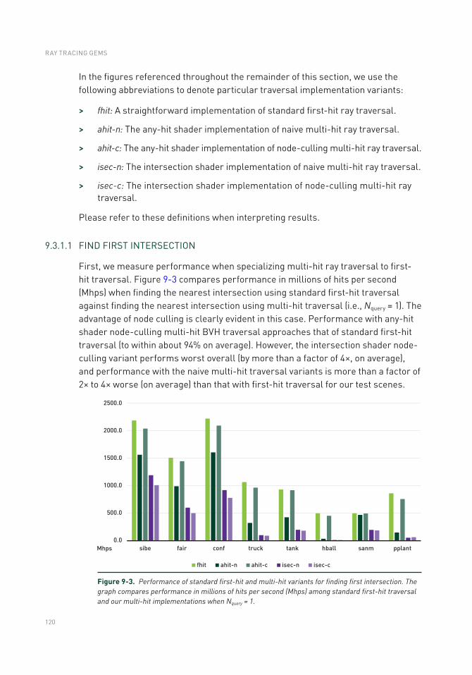
120
In the figures referenced throughout the remainder of this section, we use the following abbreviations to denote particular traversal implementation variants:
> fhit: A straightforward implementation of standard first-hit ray traversal.
> ahit-n: The any-hit shader implementation of naive multi-hit ray traversal.
> ahit-c: The any-hit shader implementation of node-culling multi-hit ray traversal.
> isec-n: The intersection shader implementation of naive multi-hit ray traversal.
> isec-c: The intersection shader implementation of node-culling multi- hit ray traversal.
Please refer to these definitions when interpreting results.
9.3.1.1 FIND FIRST INTERSECTION
First, we measure performance when specializing multi-hit ray traversal to first-hit traversal. Figure 9-3 compares performance in millions of hits per second (Mhps) when finding the nearest intersection using standard first-hit traversal against finding the nearest intersection using multi-hit traversal (i.e., Nquery = 1). The advantage of node culling is clearly evident in this case. Performance with any-hit shader node-culling multi-hit BVH traversal approaches that of standard first-hit traversal (to within about 94% on average). However, the intersection shader node-culling variant performs worst overall (by more than a factor of 4×, on average), and performance with the naive multi- hit traversal variants is more than a factor of 2× to 4× worse (on average) than that with first-hit traversal for our test scenes.
Figure 9-3. Performance of standard first-hit and multi-hit variants for finding first intersection. The graph compares performance in millions of hits per second (Mhps) among standard first-hit traversal and our multi-hit implementations when Nquery = 1.
RAY TRACING GEMS
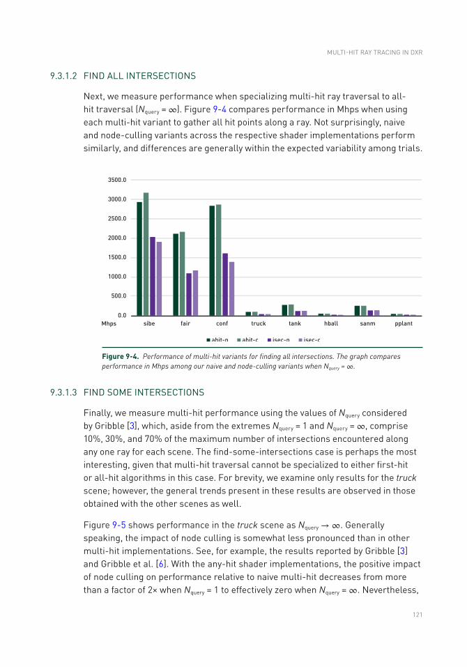
121
9.3.1.2 FIND ALL INTERSECTIONS
Next, we measure performance when specializing multi-hit ray traversal to all-hit traversal (Nquery = ∞). Figure 9-4 compares performance in Mhps when using each multi-hit variant to gather all hit points along a ray. Not surprisingly, naive and node- culling variants across the respective shader implementations perform similarly, and differences are generally within the expected variability among trials.
Figure 9-4. Performance of multi-hit variants for finding all intersections. The graph compares performance in Mhps among our naive and node-culling variants when Nquery = ∞.
9.3.1.3 FIND SOME INTERSECTIONS
Finally, we measure multi-hit performance using the values of Nquery considered by Gribble [3], which, aside from the extremes Nquery = 1 and Nquery = ∞, comprise 10%, 30%, and 70% of the maximum number of intersections encountered along any one ray for each scene. The find-some-intersections case is perhaps the most interesting, given that multi-hit traversal cannot be specialized to either first-hit or all-hit algorithms in this case. For brevity, we examine only results for the truck scene; however, the general trends present in these results are observed in those obtained with the other scenes as well.
Figure 9-5 shows performance in the truck scene as Nquery → ∞. Generally speaking, the impact of node culling is somewhat less pronounced than in other multi-hit implementations. See, for example, the results reported by Gribble [3] and Gribble et al. [6]. With the any-hit shader implementations, the positive impact of node culling on performance relative to naive multi-hit decreases from more than a factor of 2× when Nquery = 1 to effectively zero when Nquery = ∞. Nevertheless,
MULTI-HIT RAy TRACING IN DXR
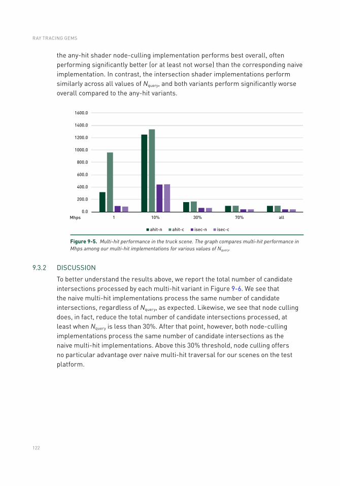
122
the any-hit shader node- culling implementation performs best overall, often performing significantly better (or at least not worse) than the corresponding naive implementation. In contrast, the intersection shader implementations perform similarly across all values of Nquery, and both variants perform significantly worse overall compared to the any-hit variants.
Figure 9-5. Multi-hit performance in the truck scene. The graph compares multi- hit performance in Mhps among our multi-hit implementations for various values of Nquery.
9.3.2 DISCUSSION
To better understand the results above, we report the total number of candidate intersections processed by each multi-hit variant in Figure 9-6. We see that the naive multi-hit implementations process the same number of candidate intersections, regardless of Nquery, as expected. Likewise, we see that node culling does, in fact, reduce the total number of candidate intersections processed, at least when Nquery is less than 30%. After that point, however, both node-culling implementations process the same number of candidate intersections as the naive multi-hit implementations. Above this 30% threshold, node culling offers no particular advantage over naive multi-hit traversal for our scenes on the test platform.
RAY TRACING GEMS
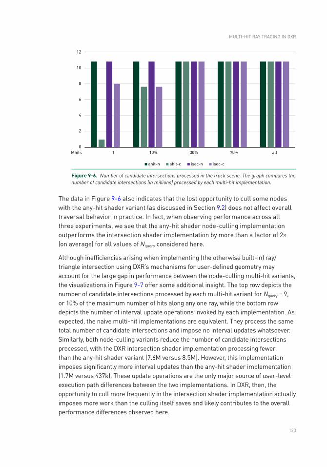
123
The data in Figure 9-6 also indicates that the lost opportunity to cull some nodes with the any-hit shader variant (as discussed in Section 9.2) does not affect overall traversal behavior in practice. In fact, when observing performance across all three experiments, we see that the any-hit shader node-culling implementation outperforms the intersection shader implementation by more than a factor of 2× (on average) for all values of Nquery considered here.
Although inefficiencies arising when implementing (the otherwise built-in) ray/triangle intersection using DXR’s mechanisms for user-defined geometry may account for the large gap in performance between the node-culling multi-hit variants, the visualizations in Figure 9-7 offer some additional insight. The top row depicts the number of candidate intersections processed by each multi-hit variant for Nquery = 9, or 10% of the maximum number of hits along any one ray, while the bottom row depicts the number of interval update operations invoked by each implementation. As expected, the naive multi-hit implementations are equivalent. They process the same total number of candidate intersections and impose no interval updates whatsoever. Similarly, both node-culling variants reduce the number of candidate intersections processed, with the DXR intersection shader implementation processing fewer than the any-hit shader variant (7.6M versus 8.5M). However, this implementation imposes significantly more interval updates than the any-hit shader implementation (1.7M versus 437k). These update operations are the only major source of user-level execution path differences between the two implementations. In DXR, then, the opportunity to cull more frequently in the intersection shader implementation actually imposes more work than the culling itself saves and likely contributes to the overall performance differences observed here.
Figure 9-6. Number of candidate intersections processed in the truck scene. The graph compares the number of candidate intersections (in millions) processed by each multi-hit implementation.
MULTI-HIT RAy TRACING IN DXR
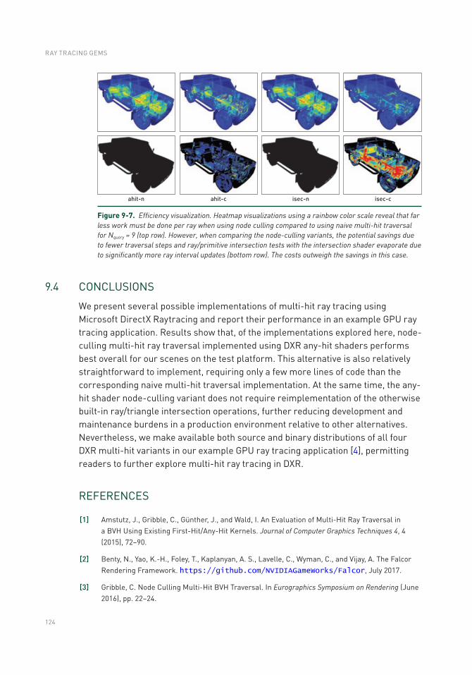
124
9.4 CONCLUSIONS
We present several possible implementations of multi-hit ray tracing using Microsoft DirectX Raytracing and report their performance in an example GPU ray tracing application. Results show that, of the implementations explored here, node-culling multi-hit ray traversal implemented using DXR any-hit shaders performs best overall for our scenes on the test platform. This alternative is also relatively straightforward to implement, requiring only a few more lines of code than the corresponding naive multi- hit traversal implementation. At the same time, the any-hit shader node-culling variant does not require reimplementation of the otherwise built-in ray/triangle intersection operations, further reducing development and maintenance burdens in a production environment relative to other alternatives. Nevertheless, we make available both source and binary distributions of all four DXR multi-hit variants in our example GPU ray tracing application [4], permitting readers to further explore multi-hit ray tracing in DXR.
REFERENCES
[1] Amstutz, J., Gribble, C., Günther, J., and Wald, I. An Evaluation of Multi-Hit Ray Traversal in a BVH Using Existing First-Hit/Any-Hit Kernels. Journal of Computer Graphics Techniques 4, 4 (2015), 72–90.
[2] Benty, N., yao, K.-H., Foley, T., Kaplanyan, A. S., Lavelle, C., Wyman, C., and Vijay, A. The Falcor Rendering Framework. https://github.com/NVIDIAGameWorks/Falcor, July 2017.
[3] Gribble, C. Node Culling Multi-Hit BVH Traversal. In Eurographics Symposium on Rendering (June 2016), pp. 22–24.
Figure 9-7. Efficiency visualization. Heatmap visualizations using a rainbow color scale reveal that far less work must be done per ray when using node culling compared to using naive multi-hit traversal for Nquery = 9 (top row). However, when comparing the node-culling variants, the potential savings due to fewer traversal steps and ray/primitive intersection tests with the intersection shader evaporate due to significantly more ray interval updates (bottom row). The costs outweigh the savings in this case.
RAY TRACING GEMS

125
[4] Gribble, C. DXR Multi-Hit Ray Tracing, October 2018. http://www.rtvtk.org/~cgribble/research/DXR-MultiHitRayTracing. Last accessed October 15, 2018.
[5] Gribble, C., Naveros, A., and Kerzner, E. Multi-Hit Ray Traversal. Journal of Computer Graphics Techniques 3, 1 (2014), 1–17.
[6] Gribble, C., Wald, I., and Amstutz, J. Implementing Node Culling Multi-Hit BVH Traversal in Embree. Journal of Computer Graphics Techniques 5, 4 (2016), 1–7.
[7] Wald, I., Amstutz, J., and Benthin, C. Robust Iterative Find-Next Ray Traversal. In Eurographics Symposium on Parallel Graphics and Visualization (2018), pp. 25–32.
[8] Wyman, C. A Gentle Introduction to DirectX Raytracing, August 2018. Original code linked from http://cwyman.org/code/dxrTutors/dxr_tutors.md.html; newer code available via https://github.com/NVIDIAGameWorks/GettingStartedWithRTXRayTracing. Last accessed November 12, 2018.
Open Access This chapter is licensed under the terms of the Creative Commons Attribution-NonCommercial-NoDerivatives 4.0 International License (http://creativecommons.org/licenses/by-nc-nd/4.0/), which permits any noncommercial use, sharing, distribution and
reproduction in any medium or format, as long as you give appropriate credit to the original author(s) and the source, provide a link to the Creative Commons license and indicate if you modified the licensed material. you do not have permission under this license to share adapted material derived from this chapter or parts of it.
The images or other third party material in this chapter are included in the chapter's Creative Commons license, unless indicated otherwise in a credit line to the material. If material is not included in the chapter's Creative Commons license and your intended use is not permitted by statutory regulation or exceeds the permitted use, you will need to obtain permission directly from the copyright holder.
MULTI-HIT RAy TRACING IN DXR
127© NVIDIA 2019 E. Haines, T. Akenine-Möller (eds.), Ray Tracing Gems, https://doi.org/10.1007/978-1-4842-4427-2_10
CHAPTER 10
A Simple Load-Balancing Scheme with High Scaling EfficiencyDietger van Antwerpen, Daniel Seibert, and Alexander KellerNVIDIA
ABSTRACT
This chapter describes an image partitioning scheme that can be used to distribute the work of computing pixel values across multiple processing units. The resulting workload distribution scheme is simple to implement, yet effective.
10.1 INTRODUCTION
A key question in attempts to distribute the rendering of a single image frame over a number of processing units is how to assign pixels to processing units. In the context of this chapter, we will use an abstract notion of a processing unit or processor. For example, a processor could be a GPU, a CPU core, or a host in a cluster of networked machines. A number of processors of various types will generally be combined into some form of rendering system or cluster.
This chapter is motivated by the workloads commonly found in path tracing renderers, which simulate the interaction of light with the materials in a scene. Light is often reflected and refracted multiple times before a light transport path is completed. The number of bounces, as well as the cost of evaluating each material, varies dramatically among different areas of a scene.
Consider, for example, a car in an infinite environment dome. Rays that miss all geometry and immediately hit the environment are extremely cheap to compute. In contrast, rays that hit a headlight of the car will incur higher ray tracing costs and will bounce around the reflectors of the headlight dozens of times before reaching the emitters of the headlight or exiting to the environment. Pixels that cover the headlight may thus be orders of magnitude more costly to compute than pixels that show only the environment. Crucially, this cost is not known a priori and thus cannot be taken into account to compute the optimal distribution of work.

128
10.2 REQUIREMENTS
An effective load balancing scheme yields good scaling over many processors. Computation and communication overhead should be low so as not to negate speedups from a small number of processors. In the interest of simplicity, it is often desirable to assign a fixed subset of the workload to each processor. While the size of the subset may be adapted over time, e.g., based on performance measurements, this re-balancing generally happens between frames. Doing so yields a scheme that is static for each frame, which makes it easier to reduce the amount of communication between the load balancer and the processors. A proper distribution of work is crucial to achieving efficient scaling with a static scheme. Each processor should be assigned a fraction of the work that is proportional to the processor’s relative performance. This is a nontrivial task when generating images using ray tracing, especially for physically based path tracing and similar techniques. The situation is further complicated in heterogeneous computing setups, where the processing power of the various processors varies dramatically. This is a common occurrence in consumer machines that combine GPUs from different generations with a CPU and in network clusters.
10.3 LOAD BALANCING
We will now consider a series of partitioning schemes and investigate their suitability for efficient workload distribution in the context we have described. For illustration, we will distribute the work among four processors, e.g., four GPUs on a single machine. Note, however, that the approaches described below apply to any number and type of processors, including combinations of different processor types.
10.3.1 NAIVE TILING
It is not uncommon for multi-GPU rasterization approaches to simply divide the image into large tiles, assigning one tile to each processor as illustrated on the left in Figure 10- 1. In our setting, this naive approach has the severe drawback that the cost of pixels is generally not distributed uniformly across the image. On the left in Figure 10-1, the cost of computing the tile on the bottom left will likely dominate the overall render time of the frame due to the expensive simulation of the headlight. All other processors will be idle for a significant portion of the frame time while the processor responsible for the blue tile finishes its work.
RAY TRACING GEMS
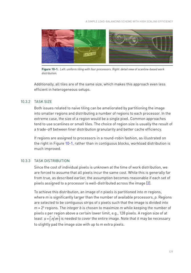
129
Additionally, all tiles are of the same size, which makes this approach even less efficient in heterogeneous setups.
10.3.2 TASK SIZE
Both issues related to naive tiling can be ameliorated by partitioning the image into smaller regions and distributing a number of regions to each processor. In the extreme case, the size of a region would be a single pixel. Common approaches tend to use scanlines or small tiles. The choice of region size is usually the result of a trade-off between finer distribution granularity and better cache efficiency.
If regions are assigned to processors in a round-robin fashion, as illustrated on the right in Figure 10-1, rather than in contiguous blocks, workload distribution is much improved.
10.3.3 TASK DISTRIBUTION
Since the cost of individual pixels is unknown at the time of work distribution, we are forced to assume that all pixels incur the same cost. While this is generally far from true, as described earlier, the assumption becomes reasonable if each set of pixels assigned to a processor is well-distributed across the image [2].
To achieve this distribution, an image of n pixels is partitioned into m regions, where m is significantly larger than the number of available processors, p. Regions are selected to be contiguous strips of s pixels such that the image is divided into m = 2b regions. The integer b is chosen to maximize m while keeping the number of pixels s per region above a certain lower limit, e.g., 128 pixels. A region size of at least s n m= é ùê ú is needed to cover the entire image. Note that it may be necessary to slightly pad the image size with up to m extra pixels.
Figure 10-1. Left: uniform tiling with four processors. Right: detail view of scanline-based work distribution.
A SIMPLE LOAD-BALANCING SCHEME WITH HIGH SCALING EFFICIENCy
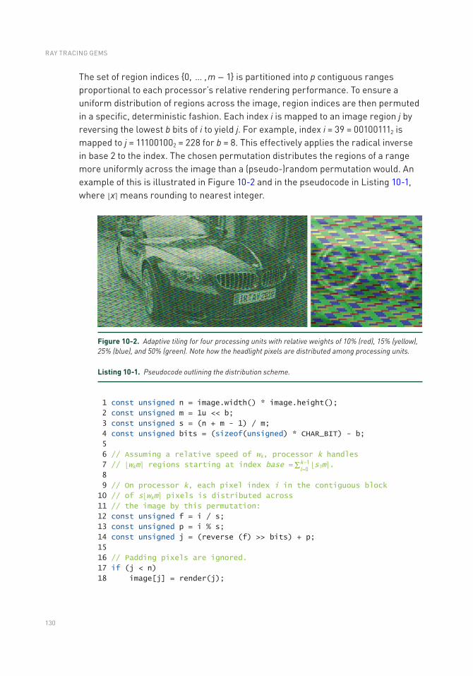
130
The set of region indices 0, … , m − 1 is partitioned into p contiguous ranges proportional to each processor’s relative rendering performance. To ensure a uniform distribution of regions across the image, region indices are then permuted in a specific, deterministic fashion. Each index i is mapped to an image region j by reversing the lowest b bits of i to yield j. For example, index i = 39 = 001001112 is mapped to j = 111001002 = 228 for b = 8. This effectively applies the radical inverse in base 2 to the index. The chosen permutation distributes the regions of a range more uniformly across the image than a (pseudo-)random permutation would. An example of this is illustrated in Figure 10-2 and in the pseudocode in Listing 10-1, where ⌊x⌉ means rounding to nearest integer.
Figure 10-2. Adaptive tiling for four processing units with relative weights of 10% (red), 15% (yellow), 25% (blue), and 50% (green). Note how the headlight pixels are distributed among processing units.
Listing 10-1. Pseudocode outlining the distribution scheme.
1 const unsigned n = image.width() * image.height();
2 const unsigned m = 1u << b;
3 const unsigned s = (n + m - 1) / m;
4 const unsigned bits = (sizeof(unsigned) * CHAR_BIT) - b;
5
6 // Assuming a relative speed of wk, processor k handles
7 // ⌊wkm⌉ regions starting at index base = kl
10-=S ⌊slm⌉.
8
9 // On processor k, each pixel index i in the contiguous block
10 // of s⌊wkm⌉ pixels is distributed across11 // the image by this permutation:
12 const unsigned f = i / s;
13 const unsigned p = i % s;
14 const unsigned j = (reverse (f) >> bits) + p;
15
16 // Padding pixels are ignored.
17 if (j < n)
18 image[j] = render(j);
RAY TRACING GEMS
131
The bit reversal function used in the permutation is cheap to compute and does not require any permutation tables to be communicated to the processors. In addition to the straightforward way, bit reversal can be implemented using masks [1], as shown in Listing 10-2. Furthermore, CUDA makes this functionality available in the form of the __brev intrinsic.
Listing 10-2. Bit reversal implementation using masks.
1 unsigned reverse(unsigned x) // Assuming 32 bit integers
2
3 x = ((x & 0xaaaaaaaa) >> 1) | ((x & 0x55555555) << 1);
4 x = ((x & 0xcccccccc) >> 2) | ((x & 0x33333333) << 2);
5 x = ((x & 0xf0f0f0f0) >> 4) | ((x & 0x0f0f0f0f) << 4);
6 x = ((x & 0xff00ff00) >> 8) | ((x & 0x00ff00ff) << 8);
7 return (x >> 16) | (x << 16);
8
For production scenes, the regions are unlikely to correlate strongly with image features due to differing shapes. As a result, the pixels assigned to each processor are expected to cover a representative portion of the image. This ensures that the cost of a task becomes roughly proportional to the number of pixels in the task, resulting in uniform load balancing.
10.3.4 IMAGE ASSEMBLy
In some specialized contexts, such as network rendering, it is undesirable to allocate and transfer the entire framebuffer from each host to a master host. The approach described in Section 10.3.3 is easily adapted to cater to this by allocating only the necessary number of pixels on each host, i.e., s ⌊wkm⌉. Line 18 of Listing 10-1 is simply changed to write to image[i-base] instead of image[j].
A display image is assembled from these permuted local framebuffers. First, the contiguous pixel ranges from all processors are concatenated into a single master framebuffer on the master processor. Then, the permutation is reversed, yielding the final image. Note that the bit reversal function is involutory, i.e., its own inverse. This property allows for efficient in-place reconstruction of the framebuffer from the permuted framebuffer, which is shown in Listing 10-3.1
1 Note the use of the same reverse function in both the distribution (Listing 10-1) and the reassembly of the image (Listing 10-3).
A SIMPLE LOAD-BALANCING SCHEME WITH HIGH SCALING EFFICIENCy
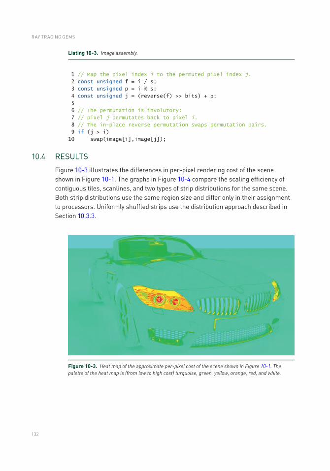
132
Listing 10-3. Image assembly.
1 // Map the pixel index i to the permuted pixel index j.
2 const unsigned f = i / s;
3 const unsigned p = i % s;
4 const unsigned j = (reverse(f) >> bits) + p;
5
6 // The permutation is involutory:
7 // pixel j permutates back to pixel i.
8 // The in-place reverse permutation swaps permutation pairs.
9 if (j > i)
10 swap(image[i],image[j]);
10.4 RESULTS
Figure 10-3 illustrates the differences in per-pixel rendering cost of the scene shown in Figure 10-1. The graphs in Figure 10-4 compare the scaling efficiency of contiguous tiles, scanlines, and two types of strip distributions for the same scene. Both strip distributions use the same region size and differ only in their assignment to processors. Uniformly shuffled strips use the distribution approach described in Section 10.3.3.
Figure 10-3. Heat map of the approximate per-pixel cost of the scene shown in Figure 10-1. The palette of the heat map is (from low to high cost) turquoise, green, yellow, orange, red, and white.
RAY TRACING GEMS
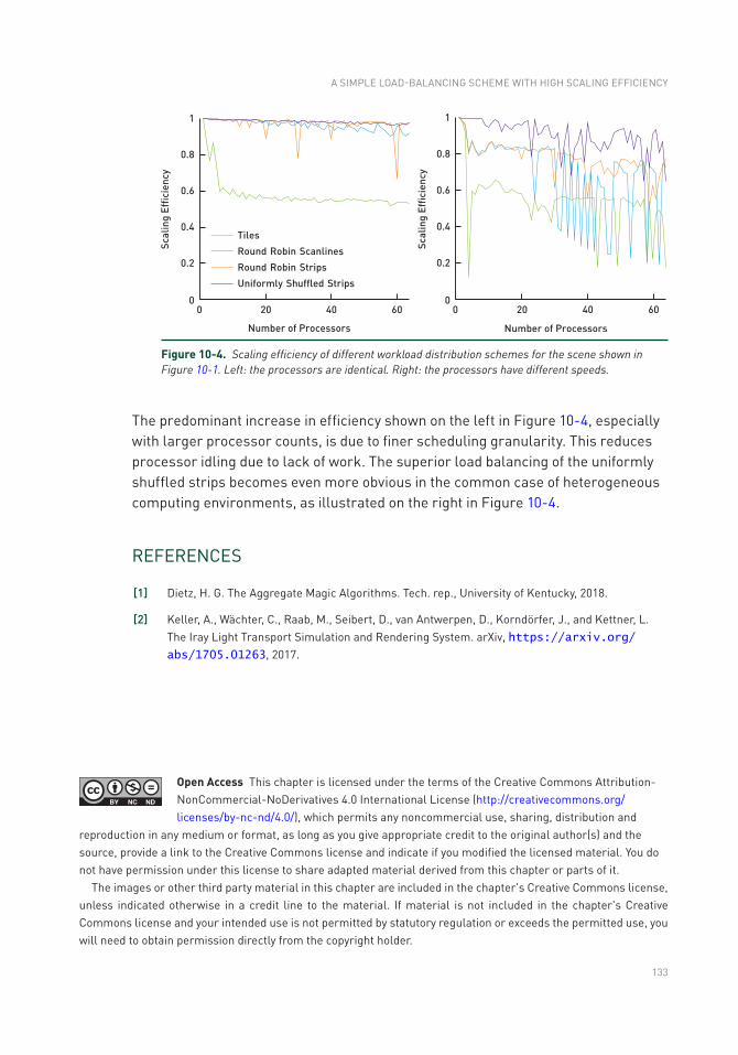
133
The predominant increase in efficiency shown on the left in Figure 10-4, especially with larger processor counts, is due to finer scheduling granularity. This reduces processor idling due to lack of work. The superior load balancing of the uniformly shuffled strips becomes even more obvious in the common case of heterogeneous computing environments, as illustrated on the right in Figure 10-4.
REFERENCES
[1] Dietz, H. G. The Aggregate Magic Algorithms. Tech. rep., University of Kentucky, 2018.
[2] Keller, A., Wächter, C., Raab, M., Seibert, D., van Antwerpen, D., Korndörfer, J., and Kettner, L. The Iray Light Transport Simulation and Rendering System. arXiv, https://arxiv.org/abs/1705.01263, 2017.
Figure 10-4. Scaling efficiency of different workload distribution schemes for the scene shown in Figure 10-1. Left: the processors are identical. Right: the processors have different speeds.
Open Access This chapter is licensed under the terms of the Creative Commons Attribution-NonCommercial-NoDerivatives 4.0 International License (http://creativecommons.org/licenses/by-nc-nd/4.0/), which permits any noncommercial use, sharing, distribution and
reproduction in any medium or format, as long as you give appropriate credit to the original author(s) and the source, provide a link to the Creative Commons license and indicate if you modified the licensed material. you do not have permission under this license to share adapted material derived from this chapter or parts of it.
The images or other third party material in this chapter are included in the chapter's Creative Commons license, unless indicated otherwise in a credit line to the material. If material is not included in the chapter's Creative Commons license and your intended use is not permitted by statutory regulation or exceeds the permitted use, you will need to obtain permission directly from the copyright holder.
A SIMPLE LOAD-BALANCING SCHEME WITH HIGH SCALING EFFICIENCy
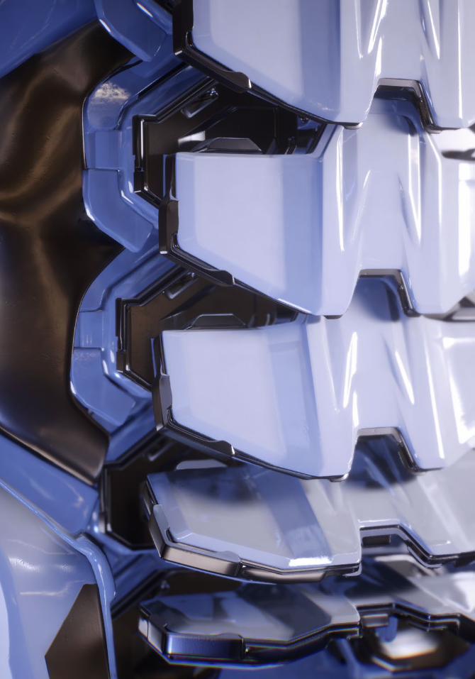
PART III
REFLECTIONS, REFRACTIONS, AND SHADOWS
137
PART III
Reflections, Refractions, and Shadows
Any ray traced rendering leads to several design decisions about what effects are supported and how they are supported. Ray tracing’s main historical appeal is that it handles shadows, reflections, and refractions well. However, when you sit down and actually implement a system that supports these effects, you run into several non-obvious design decisions. This part of the book describes several specific approaches to some of these.
Though ray tracing a clear glass ball is straightforward, more complex models throw a wrench in the works. For example, a simple glass of water presents three distinct types of material interface behaviors: water/air, glass/air, and glass/water. To get the refraction right, a ray/surface interaction needs to know not only which interface is hit but also what material is on what side of the ray. It is problematic to expect an artist to build a model out of these interfaces; imagine filling a glass with water. A clever and battle-tested approach to dealing with the issue is described in Chapter 11, “Automatic Handling of Materials in Nested Volumes.”
An issue that has plagued almost all ray tracing programs is what to do when a bump map produces physically impossible surface normal vectors. The obvious “hard if” code solution to ignore these can cause jarring color discontinuities. Every ray tracer has its own home-grown hack to deal with this. In Chapter 12, “A Microfacet-Based Shadowing Function to Solve the Bump Terminator Problem,” a simple statistical approach with a clean implementation is presented.
Ray tracing’s screen-space approach has made it particularly strong at generating screen-accurate shadows without all the aliasing problems associated with shadow maps. However, can ray tracing be made fast enough to be interactive? Chapter 13, “Ray Traced Shadows: Maintaining Real-Time Frame Rates,” provides a detailed explanation of how this can be done.
Most simple ray tracers send rays from the eye. Typically these programs cannot practically generate caustics, the focused light patterns that we associate with glasses of liquid, swimming pools, and lakes. The “practically” is because the results are too noisy. However, sending rays from the light into the environment

138
is a workable approach to generate caustics. In fact, this can even be done in real time, as described in Chapter 14, “Ray-Guided Volumetric Water Caustics in Single Scattering Media with DXR.”
In summary, a basic ray tracer is fairly straightforward. Deploying a production ray tracer requires some careful handling of basic effects, and this part provides several useful approaches for doing just that.
Peter Shirley
139© NVIDIA 2019 E. Haines, T. Akenine-Möller (eds.), Ray Tracing Gems, https://doi.org/10.1007/978-1-4842-4427-2_11
CHAPTER 11
Automatic Handling of Materials in Nested VolumesCarsten Wächter and Matthias Raab NVIDIA
ABSTRACT
We present a novel and simple algorithm to automatically handle nested volumes and transitions between volumes, enabling push-button rendering functionality. The only requirements are the use of closed, watertight volumes (along with a ray tracing implementation such as NVIDIA RTX that guarantees watertight traversal and intersection) and that neighboring volumes are not intended to intersect each other, except for a small overlap that actually will model the boundary between the volumes.
11.1 MODELING VOLUMES
Brute-force path tracing has become a core technique to simulate light transport and is used to render realistic images in many of the large production rendering systems [1, 2]. For any renderer based on ray tracing, it is necessary to handle the relationship of materials and geometric objects in a scene:
> To correctly simulate reflection and refraction, the indices of refraction on the front- and backface of a surface need to be known. Note that this is not only needed for materials featuring refraction, but also in cases where the intensity of a reflection is driven by Fresnel equations.
> The volume coefficients (scattering and absorption) may need to be determined, e.g., to apply volume attenuation when a ray leaves an absorbing volume.
Thus, handling volumetric data, including nested media, is an essential requirement to render production scenes and must be tightly integrated into the rendering core. Ray tracing, i.e., its underlying hierarchy traversal and geometry intersection, is always affected by the limits of the floating-point precision implementation. Even the geometrical data representation, e.g., instancing of meshes using floating-point transformations, introduces further precision issues. Therefore, handling volume transitions robustly at least requires careful modeling of the volumes and their surrounding hull geometry. In the following we will distinguish three cases to model neighboring volumes. See Figure 11-1.
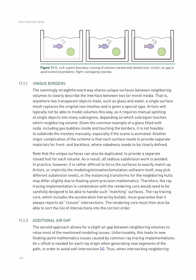
140
11.1.1 UNIQUE BORDERS
The seemingly straightforward way shares unique surfaces between neighboring volumes to clearly describe the interface between two (or more) media. That is, anywhere two transparent objects meet, such as glass and water, a single surface mesh replaces the original two meshes and is given a special type. Artists will typically not be able to model volumes this way, as it requires manual splitting of single objects into many subregions, depending on which subregion touches which neighboring volume. Given the common example of a glass filled with soda, including gas bubbles inside and touching the borders, it is not feasible to subdivide the meshes manually, especially if the scene is animated. Another major complication of the scheme is that each surface needs to provide separate materials for front- and backface, where sidedness needs to be clearly defined.
Note that the unique surfaces can also be duplicated, to provide a separate closed hull for each volume. As a result, all tedious subdivision work is avoided. In practice, however, it is rather difficult to force the surfaces to exactly match up. Artists, or implicitly the modeling/animation/simulation software itself, may pick different subdivision levels, or the instancing transforms for the neighboring hulls may differ slightly due to floating-point precision mathematics. Therefore, the ray tracing implementation in combination with the rendering core would need to be carefully designed to be able to handle such “matching” surfaces. The ray tracing core, which includes the acceleration hierarchy builder, must guarantee that it always reports all “closest” intersections. The rendering core must then also be able to sort the list of intersections into the correct order.
11.1.2 ADDITIONAL AIR GAP
The second approach allows for a slight air gap between neighboring volumes to relax most of the mentioned modeling issues. Unfortunately, this leads to new floating-point mathematics issues caused by common ray tracing implementations: An ϵ offset is needed for each ray origin when generating new segments of the path, in order to avoid self-intersection [4]. Thus, when intersecting neighboring
Figure 11-1. Left: explicit boundary crossing of volumes marked with dashed lines. Center: air gap to avoid numerical problems. Right: overlapping volumes.
RAY TRACING GEMS
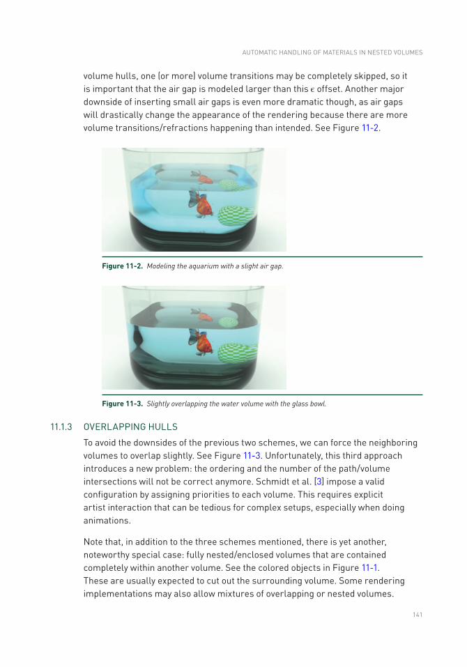
141
volume hulls, one (or more) volume transitions may be completely skipped, so it is important that the air gap is modeled larger than this ϵ offset. Another major downside of inserting small air gaps is even more dramatic though, as air gaps will drastically change the appearance of the rendering because there are more volume transitions/refractions happening than intended. See Figure 11-2.
Figure 11-2. Modeling the aquarium with a slight air gap.
Figure 11-3. Slightly overlapping the water volume with the glass bowl.
11.1.3 OVERLAPPING HULLS
To avoid the downsides of the previous two schemes, we can force the neighboring volumes to overlap slightly. See Figure 11-3. Unfortunately, this third approach introduces a new problem: the ordering and the number of the path/volume intersections will not be correct anymore. Schmidt et al. [3] impose a valid configuration by assigning priorities to each volume. This requires explicit artist interaction that can be tedious for complex setups, especially when doing animations.
Note that, in addition to the three schemes mentioned, there is yet another, noteworthy special case: fully nested/enclosed volumes that are contained completely within another volume. See the colored objects in Figure 11-1. These are usually expected to cut out the surrounding volume. Some rendering implementations may also allow mixtures of overlapping or nested volumes.
AUTOMATIC HANDLING OF MATERIALS IN NESTED VOLUMES
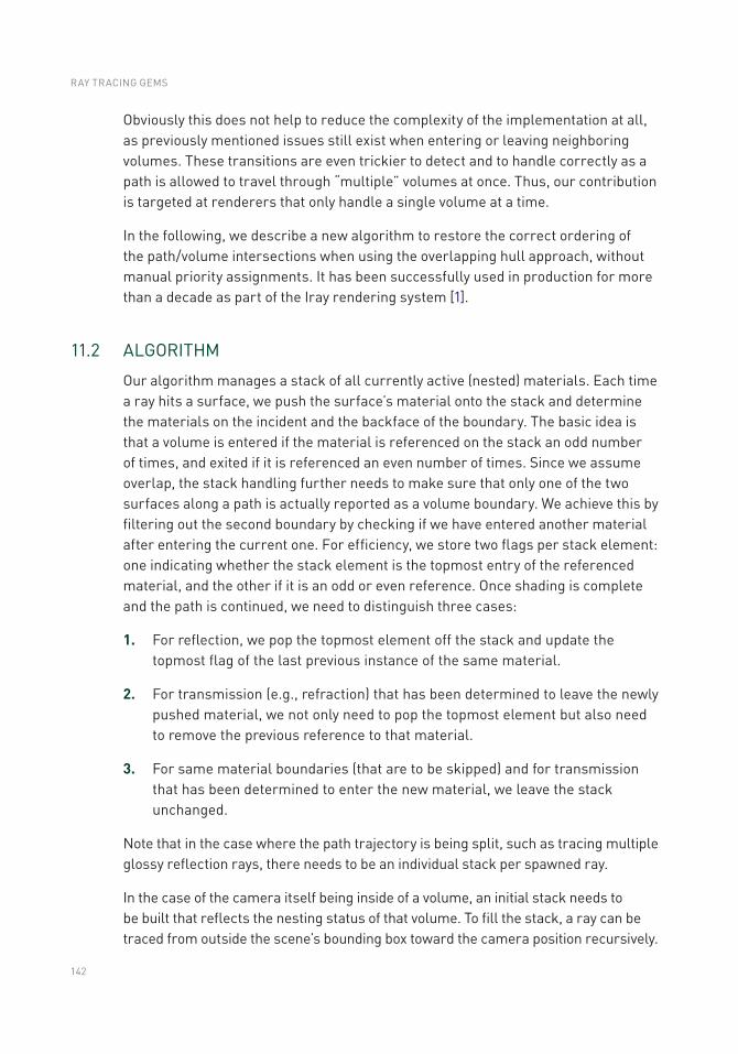
142
Obviously this does not help to reduce the complexity of the implementation at all, as previously mentioned issues still exist when entering or leaving neighboring volumes. These transitions are even trickier to detect and to handle correctly as a path is allowed to travel through “multiple” volumes at once. Thus, our contribution is targeted at renderers that only handle a single volume at a time.
In the following, we describe a new algorithm to restore the correct ordering of the path/volume intersections when using the overlapping hull approach, without manual priority assignments. It has been successfully used in production for more than a decade as part of the Iray rendering system [1].
11.2 ALGORITHM
Our algorithm manages a stack of all currently active (nested) materials. Each time a ray hits a surface, we push the surface’s material onto the stack and determine the materials on the incident and the backface of the boundary. The basic idea is that a volume is entered if the material is referenced on the stack an odd number of times, and exited if it is referenced an even number of times. Since we assume overlap, the stack handling further needs to make sure that only one of the two surfaces along a path is actually reported as a volume boundary. We achieve this by filtering out the second boundary by checking if we have entered another material after entering the current one. For efficiency, we store two flags per stack element: one indicating whether the stack element is the topmost entry of the referenced material, and the other if it is an odd or even reference. Once shading is complete and the path is continued, we need to distinguish three cases:
1. For reflection, we pop the topmost element off the stack and update the topmost flag of the last previous instance of the same material.
2. For transmission (e.g., refraction) that has been determined to leave the newly pushed material, we not only need to pop the topmost element but also need to remove the previous reference to that material.
3. For same material boundaries (that are to be skipped) and for transmission that has been determined to enter the new material, we leave the stack unchanged.
Note that in the case where the path trajectory is being split, such as tracing multiple glossy reflection rays, there needs to be an individual stack per spawned ray.
In the case of the camera itself being inside of a volume, an initial stack needs to be built that reflects the nesting status of that volume. To fill the stack, a ray can be traced from outside the scene’s bounding box toward the camera position recursively.
RAY TRACING GEMS
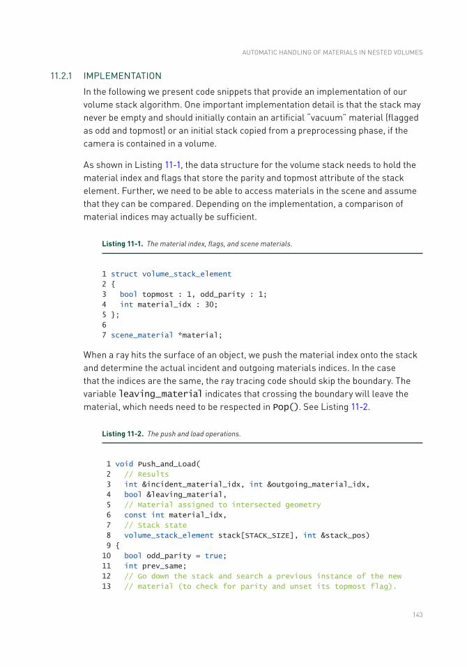
143
11.2.1 IMPLEMENTATION
In the following we present code snippets that provide an implementation of our volume stack algorithm. One important implementation detail is that the stack may never be empty and should initially contain an artificial “vacuum” material (flagged as odd and topmost) or an initial stack copied from a preprocessing phase, if the camera is contained in a volume.
As shown in Listing 11-1, the data structure for the volume stack needs to hold the material index and flags that store the parity and topmost attribute of the stack element. Further, we need to be able to access materials in the scene and assume that they can be compared. Depending on the implementation, a comparison of material indices may actually be sufficient.
Listing 11-1. The material index, flags, and scene materials.
1 struct volume_stack_element
2
3 bool topmost : 1, odd_parity : 1;
4 int material_idx : 30;
5 ;
6
7 scene_material *material;
When a ray hits the surface of an object, we push the material index onto the stack and determine the actual incident and outgoing materials indices. In the case that the indices are the same, the ray tracing code should skip the boundary. The variable leaving_material indicates that crossing the boundary will leave the material, which needs need to be respected in Pop(). See Listing 11-2.
Listing 11-2. The push and load operations.
1 void Push_and_Load(
2 // Results
3 int &incident_material_idx, int &outgoing_material_idx,
4 bool &leaving_material,
5 // Material assigned to intersected geometry
6 const int material_idx,
7 // Stack state
8 volume_stack_element stack[STACK_SIZE], int &stack_pos)
9
10 bool odd_parity = true;
11 int prev_same;
12 // Go down the stack and search a previous instance of the new
13 // material (to check for parity and unset its topmost flag).
AUTOMATIC HANDLING OF MATERIALS IN NESTED VOLUMES
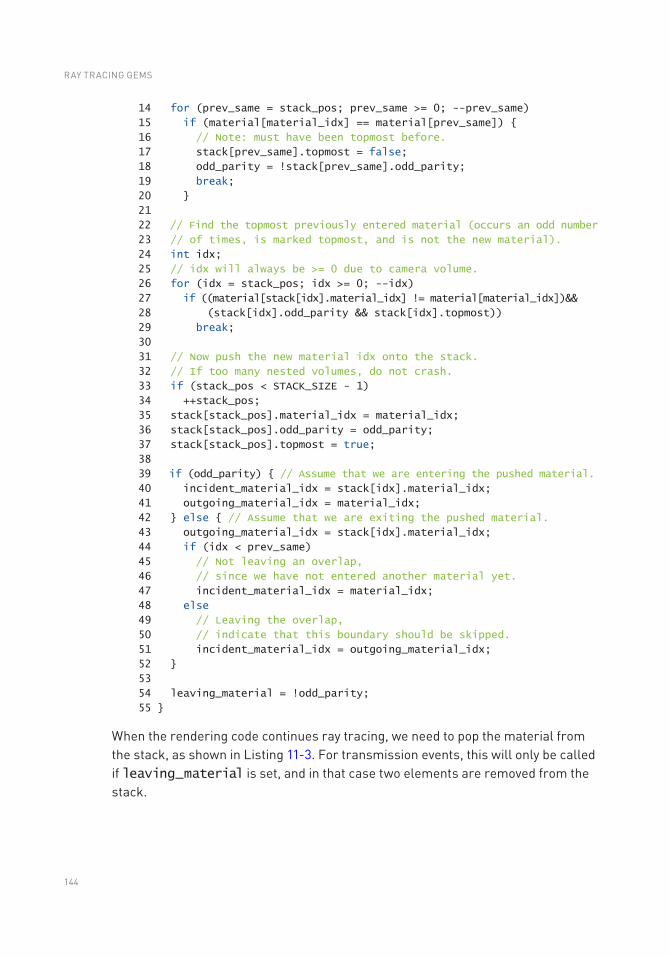
144
14 for (prev_same = stack_pos; prev_same >= 0; --prev_same)
15 if (material[material_idx] == material[prev_same])
16 // Note: must have been topmost before.
17 stack[prev_same].topmost = false;
18 odd_parity = !stack[prev_same].odd_parity;
19 break;
20
21
22 // Find the topmost previously entered material (occurs an odd number
23 // of times, is marked topmost, and is not the new material).
24 int idx;
25 // idx will always be >= 0 due to camera volume.
26 for (idx = stack_pos; idx >= 0; --idx)
27 if ((material[stack[idx].material_idx] != material[material_idx])&&
28 (stack[idx].odd_parity && stack[idx].topmost))
29 break;
30
31 // Now push the new material idx onto the stack.
32 // If too many nested volumes, do not crash.
33 if (stack_pos < STACK_SIZE - 1)
34 ++stack_pos;
35 stack[stack_pos].material_idx = material_idx;
36 stack[stack_pos].odd_parity = odd_parity;
37 stack[stack_pos].topmost = true;
38
39 if (odd_parity) // Assume that we are entering the pushed material.
40 incident_material_idx = stack[idx].material_idx;
41 outgoing_material_idx = material_idx;
42 else // Assume that we are exiting the pushed material.
43 outgoing_material_idx = stack[idx].material_idx;
44 if (idx < prev_same)
45 // Not leaving an overlap,
46 // since we have not entered another material yet.
47 incident_material_idx = material_idx;
48 else
49 // Leaving the overlap,
50 // indicate that this boundary should be skipped.
51 incident_material_idx = outgoing_material_idx;
52
53
54 leaving_material = !odd_parity;
55
When the rendering code continues ray tracing, we need to pop the material from the stack, as shown in Listing 11-3. For transmission events, this will only be called if leaving_material is set, and in that case two elements are removed from the stack.
RAY TRACING GEMS
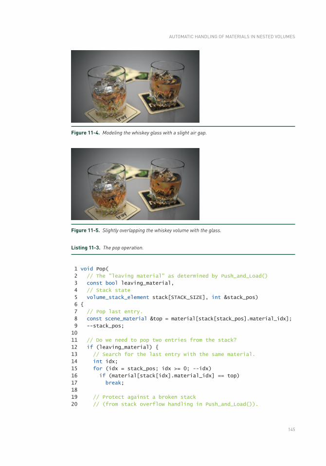
145
Listing 11-3. The pop operation.
1 void Pop(
2 // The "leaving material" as determined by Push_and_Load()
3 const bool leaving_material,
4 // Stack state
5 volume_stack_element stack[STACK_SIZE], int &stack_pos)
6
7 // Pop last entry.
8 const scene_material &top = material[stack[stack_pos].material_idx];
9 --stack_pos;
10
11 // Do we need to pop two entries from the stack?
12 if (leaving_material)
13 // Search for the last entry with the same material.
14 int idx;
15 for (idx = stack_pos; idx >= 0; --idx)
16 if (material[stack[idx].material_idx] == top)
17 break;
18
19 // Protect against a broken stack
20 // (from stack overflow handling in Push_and_Load()).
Figure 11-4. Modeling the whiskey glass with a slight air gap.
Figure 11-5. Slightly overlapping the whiskey volume with the glass.
AUTOMATIC HANDLING OF MATERIALS IN NESTED VOLUMES
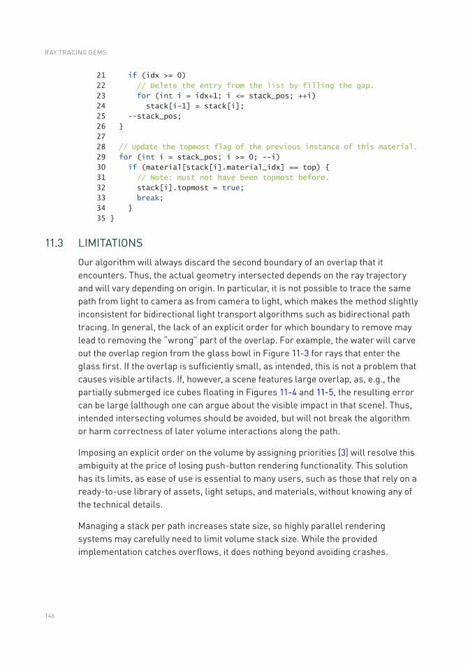
146
21 if (idx >= 0)
22 // Delete the entry from the list by filling the gap.
23 for (int i = idx+1; i <= stack_pos; ++i)
24 stack[i-1] = stack[i];
25 --stack_pos;
26
27
28 // Update the topmost flag of the previous instance of this material.
29 for (int i = stack_pos; i >= 0; --i)
30 if (material[stack[i].material_idx] == top)
31 // Note: must not have been topmost before.
32 stack[i].topmost = true;
33 break;
34
35
11.3 LIMITATIONS
Our algorithm will always discard the second boundary of an overlap that it encounters. Thus, the actual geometry intersected depends on the ray trajectory and will vary depending on origin. In particular, it is not possible to trace the same path from light to camera as from camera to light, which makes the method slightly inconsistent for bidirectional light transport algorithms such as bidirectional path tracing. In general, the lack of an explicit order for which boundary to remove may lead to removing the “wrong” part of the overlap. For example, the water will carve out the overlap region from the glass bowl in Figure 11-3 for rays that enter the glass first. If the overlap is sufficiently small, as intended, this is not a problem that causes visible artifacts. If, however, a scene features large overlap, as, e.g., the partially submerged ice cubes floating in Figures 11-4 and 11-5, the resulting error can be large (although one can argue about the visible impact in that scene). Thus, intended intersecting volumes should be avoided, but will not break the algorithm or harm correctness of later volume interactions along the path.
Imposing an explicit order on the volume by assigning priorities [3] will resolve this ambiguity at the price of losing push-button rendering functionality. This solution has its limits, as ease of use is essential to many users, such as those that rely on a ready-to-use library of assets, light setups, and materials, without knowing any of the technical details.
Managing a stack per path increases state size, so highly parallel rendering systems may carefully need to limit volume stack size. While the provided implementation catches overflows, it does nothing beyond avoiding crashes.
RAY TRACING GEMS
147
ACKNOWLEDGMENTS
An early version of this algorithm was conceived in collaboration with Leonhard Grünschloß. One part of the aquarium scene was provided by Turbosquid and the other by Autodesk.
REFERENCES
[1] Keller, A., Wächter, C., Raab, M., Seibert, D., van Antwerpen, D., Korndörfer, J., and Kettner, L. The Iray Light Transport Simulation and Rendering System. arXiv, https://arxiv.org/abs/1705.01263, 2017.
[2] Pharr, M. Special Issue On Production Rendering and Regular Papers. ACM Transactions on Graphics 37, 3 (2018).
[3] Schmidt, C. M., and Budge, B. Simple Nested Dielectrics in Ray Traced Images. Journal of Graphics Tools 7, 2 (2002), 1–8.
[4] Woo, A., Pearce, A., and Ouellette, M. It’s Really Not a Rendering Bug, You See... IEEE Computer Graphics and Applications 16, 5 (Sept 1996), 21–25.
Open Access This chapter is licensed under the terms of the Creative Commons Attribution-NonCommercial-NoDerivatives 4.0 International License (http://creativecommons.org/licenses/by-nc-nd/4.0/), which permits any noncommercial use, sharing, distribution and
reproduction in any medium or format, as long as you give appropriate credit to the original author(s) and the source, provide a link to the Creative Commons license and indicate if you modified the licensed material. You do not have permission under this license to share adapted material derived from this chapter or parts of it.
The images or other third party material in this chapter are included in the chapter's Creative Commons license, unless indicated otherwise in a credit line to the material. If material is not included in the chapter's Creative Commons license and your intended use is not permitted by statutory regulation or exceeds the permitted use, you will need to obtain permission directly from the copyright holder.
AUTOMATIC HANDLING OF MATERIALS IN NESTED VOLUMES
149© NVIDIA 2019 E. Haines, T. Akenine-Möller (eds.), Ray Tracing Gems, https://doi.org/10.1007/978-1-4842-4427-2_12
CHAPTER 12
A Microfacet-Based Shadowing Function to Solve the Bump Terminator ProblemAlejandro Conty Estevez, Pascal Lecocq, and Clifford Stein Sony Pictures Imageworks
ABSTRACT
We present a technique to hide the abrupt shadow terminator line when strong bump or normal maps are used to emulate micro-geometry. Our approach, based on microfacet shadowing functions, is simple and inexpensive. Instead of rendering detailed and expensive height-field shadows, we apply a statistical solution built on the assumption that normals follow a nearly normal random distribution. We also contribute a useful approximate variance measure for GGX, which is otherwise undefined analytically.
12.1 INTRODUCTION
Bump mapping is widely used both in real-time rendering for games and in batch rendering for cinema. It adds high-frequency detail on surfaces that would otherwise be too expensive to render with actual geometry or displacement mapping. Also, it is responsible for those last fine-grained detailed imperfections added to surfaces.
Bump mapping works as a perturbation in the normal’s orientation that does not derive from the underlying geometry but instead from a texture map or some procedural pattern. Like any other shortcut, however, it can yield unwanted artifacts—specifically the well-known hard terminator shown in Figure 12-1. This occurs because the expected smooth intensity falloff due to the changing normal is interrupted when the surface suddenly shadows the incident light rays. This problem does not appear when the normal has no perturbation since the irradiance has already dropped to zero by the time this happens. But, bump mapping has the effect of extending the light’s influence too far by tilting normals toward the incoming light direction, making the lit area cross the shadow terminator.
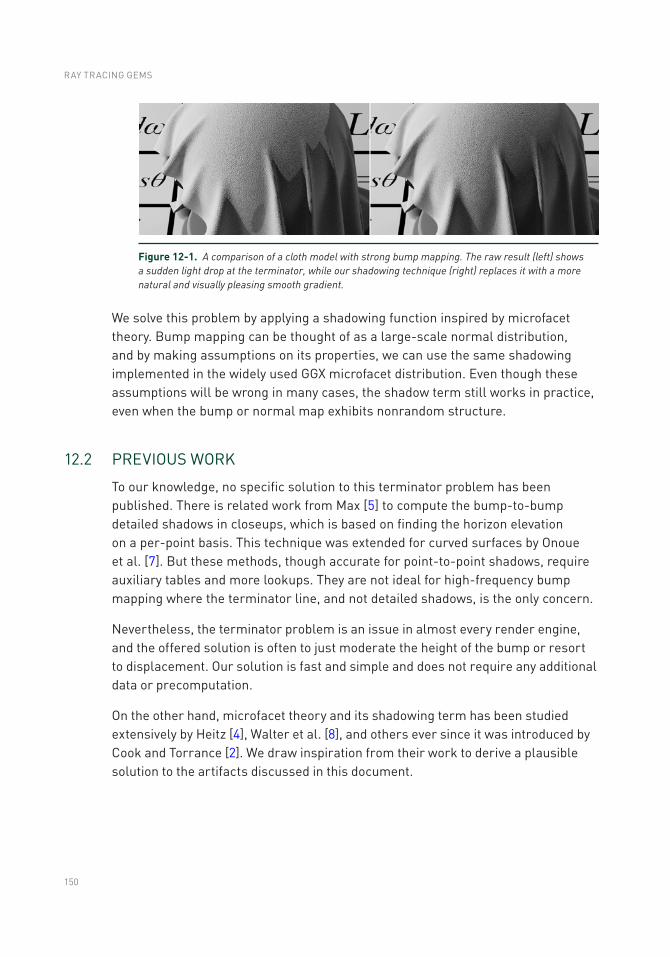
150
We solve this problem by applying a shadowing function inspired by microfacet theory. Bump mapping can be thought of as a large-scale normal distribution, and by making assumptions on its properties, we can use the same shadowing implemented in the widely used GGX microfacet distribution. Even though these assumptions will be wrong in many cases, the shadow term still works in practice, even when the bump or normal map exhibits nonrandom structure.
12.2 PREVIOUS WORK
To our knowledge, no specific solution to this terminator problem has been published. There is related work from Max [5] to compute the bump-to-bump detailed shadows in closeups, which is based on finding the horizon elevation on a per-point basis. This technique was extended for curved surfaces by Onoue et al. [7]. But these methods, though accurate for point-to-point shadows, require auxiliary tables and more lookups. They are not ideal for high-frequency bump mapping where the terminator line, and not detailed shadows, is the only concern.
Nevertheless, the terminator problem is an issue in almost every render engine, and the offered solution is often to just moderate the height of the bump or resort to displacement. Our solution is fast and simple and does not require any additional data or precomputation.
On the other hand, microfacet theory and its shadowing term has been studied extensively by Heitz [4], Walter et al. [8], and others ever since it was introduced by Cook and Torrance [2]. We draw inspiration from their work to derive a plausible solution to the artifacts discussed in this document.
Figure 12-1. A comparison of a cloth model with strong bump mapping. The raw result (left) shows a sudden light drop at the terminator, while our shadowing technique (right) replaces it with a more natural and visually pleasing smooth gradient.
RAY TRACING GEMS
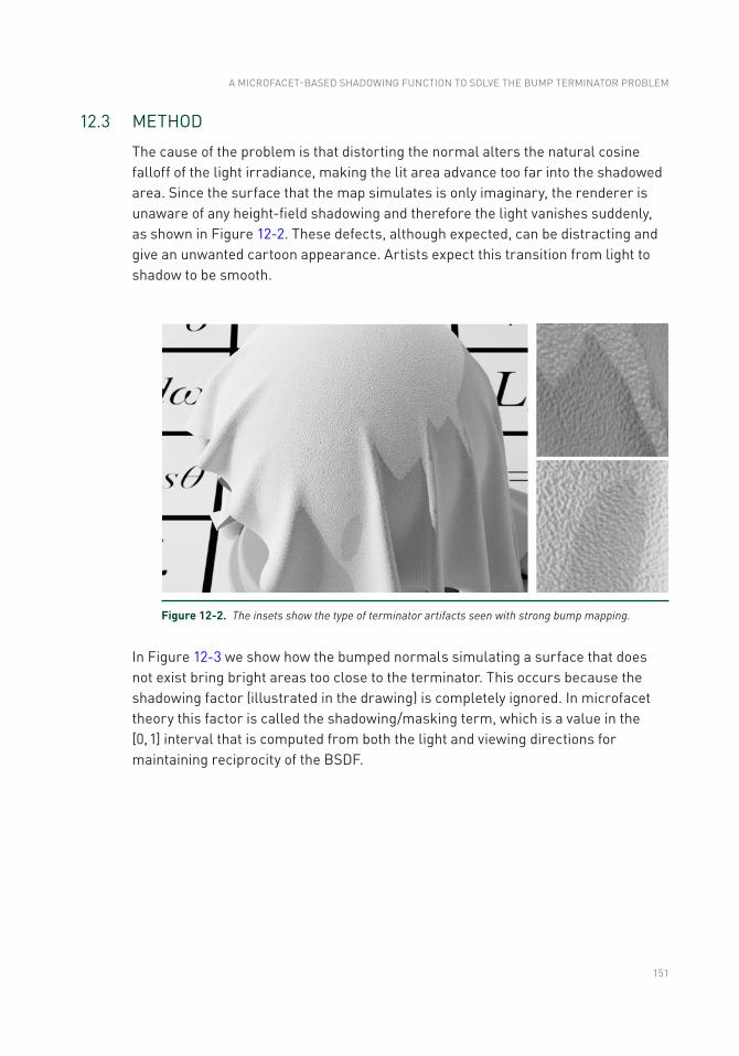
151
12.3 METHOD
The cause of the problem is that distorting the normal alters the natural cosine falloff of the light irradiance, making the lit area advance too far into the shadowed area. Since the surface that the map simulates is only imaginary, the renderer is unaware of any height-field shadowing and therefore the light vanishes suddenly, as shown in Figure 12- 2. These defects, although expected, can be distracting and give an unwanted cartoon appearance. Artists expect this transition from light to shadow to be smooth.
Figure 12-2. The insets show the type of terminator artifacts seen with strong bump mapping.
In Figure 12-3 we show how the bumped normals simulating a surface that does not exist bring bright areas too close to the terminator. This occurs because the shadowing factor (illustrated in the drawing) is completely ignored. In microfacet theory this factor is called the shadowing/masking term, which is a value in the [0, 1] interval that is computed from both the light and viewing directions for maintaining reciprocity of the BSDF.
A MICROFACET-BASED SHADOWING FUNCTION TO SOLVE THE BUMP TERMINATOR PROBLEM
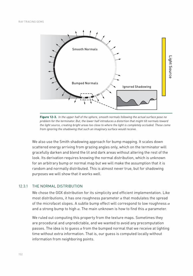
152
We also use the Smith shadowing approach for bump mapping. It scales down scattered energy arriving from grazing angles only, which on the terminator will gracefully darken and blend the lit and dark areas without altering the rest of the look. Its derivation requires knowing the normal distribution, which is unknown for an arbitrary bump or normal map but we will make the assumption that it is random and normally distributed. This is almost never true, but for shadowing purposes we will show that it works well.
12.3.1 THE NORMAL DISTRIBUTION
We chose the GGX distribution for its simplicity and efficient implementation. Like most distributions, it has one roughness parameter α that modulates the spread of the microfacet slopes. A subtle bump effect will correspond to low roughness α and a strong bump to high α. The main unknown is how to find this α parameter.
We ruled out computing this property from the texture maps. Sometimes they are procedural and unpredictable, and we wanted to avoid any precomputation passes. The idea is to guess α from the bumped normal that we receive at lighting time without extra information. That is, our guess is computed locally without information from neighboring points.
Figure 12-3. In the upper half of the sphere, smooth normals following the actual surface pose no problem for the terminator. But, the lower half introduces a distortion that might tilt normals toward the light source, creating bright areas too close to where the light is completely occluded. These come from ignoring the shadowing that such an imaginary surface would receive.
RAY TRACING GEMS
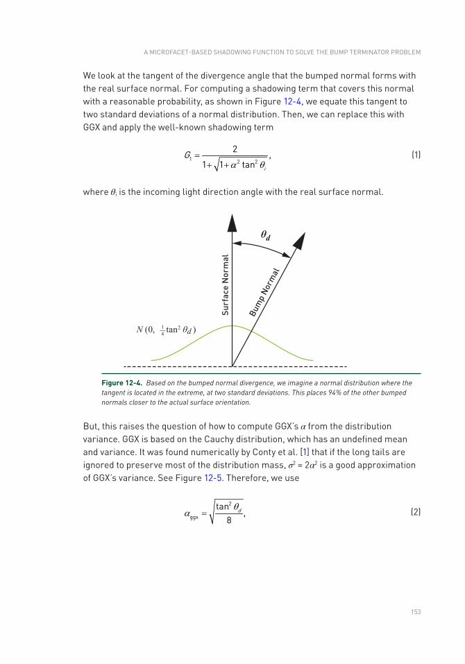
153
We look at the tangent of the divergence angle that the bumped normal forms with the real surface normal. For computing a shadowing term that covers this normal with a reasonable probability, as shown in Figure 12-4, we equate this tangent to two standard deviations of a normal distribution. Then, we can replace this with GGX and apply the well-known shadowing term
i
G1 2 2
2 ,1 1 tana q
=+ +
(1)
where θi is the incoming light direction angle with the real surface normal.
Figure 12-4. Based on the bumped normal divergence, we imagine a normal distribution where the tangent is located in the extreme, at two standard deviations. This places 94% of the other bumped normals closer to the actual surface orientation.
But, this raises the question of how to compute GGX’s α from the distribution variance. GGX is based on the Cauchy distribution, which has an undefined mean and variance. It was found numerically by Conty et al. [1] that if the long tails are ignored to preserve most of the distribution mass, σ2 = 2α2 is a good approximation of GGX’s variance. See Figure 12-5. Therefore, we use
d
2
ggx
tan,
8q
a =
(2)
A MICROFACET-BASED SHADOWING FUNCTION TO SOLVE THE BUMP TERMINATOR PROBLEM
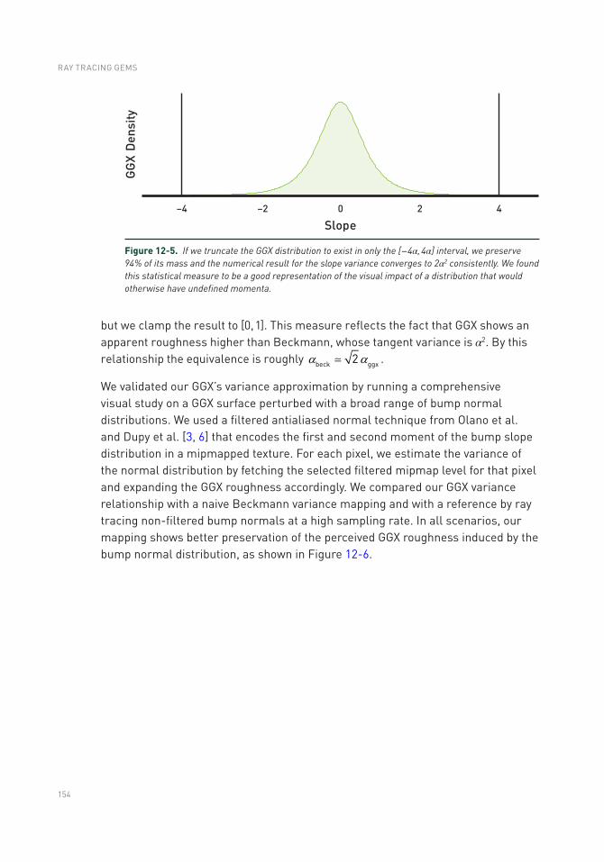
154
but we clamp the result to [0, 1]. This measure reflects the fact that GGX shows an apparent roughness higher than Beckmann, whose tangent variance is α2. By this relationship the equivalence is roughly beck ggx2a a .
We validated our GGX’s variance approximation by running a comprehensive visual study on a GGX surface perturbed with a broad range of bump normal distributions. We used a filtered antialiased normal technique from Olano et al. and Dupy et al. [3, 6] that encodes the first and second moment of the bump slope distribution in a mipmapped texture. For each pixel, we estimate the variance of the normal distribution by fetching the selected filtered mipmap level for that pixel and expanding the GGX roughness accordingly. We compared our GGX variance relationship with a naive Beckmann variance mapping and with a reference by ray tracing non-filtered bump normals at a high sampling rate. In all scenarios, our mapping shows better preservation of the perceived GGX roughness induced by the bump normal distribution, as shown in Figure 12-6.
Figure 12-5. If we truncate the GGX distribution to exist in only the [−4α, 4α] interval, we preserve 94% of its mass and the numerical result for the slope variance converges to 2α2 consistently. We found this statistical measure to be a good representation of the visual impact of a distribution that would otherwise have undefined momenta.
RAY TRACING GEMS
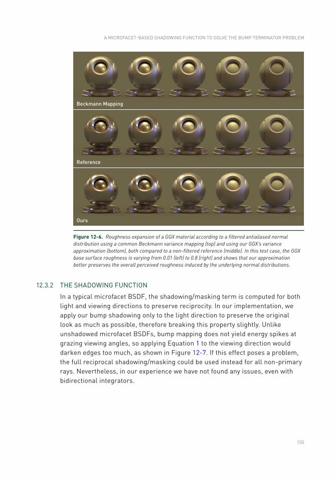
155
Figure 12-6. Roughness expansion of a GGX material according to a filtered antialiased normal distribution using a common Beckmann variance mapping (top) and using our GGX’s variance approximation (bottom), both compared to a non-filtered reference (middle). In this test case, the GGX base surface roughness is varying from 0.01 (left) to 0.8 (right) and shows that our approximation better preserves the overall perceived roughness induced by the underlying normal distributions.
12.3.2 THE SHADOWING FUNCTION
In a typical microfacet BSDF, the shadowing/masking term is computed for both light and viewing directions to preserve reciprocity. In our implementation, we apply our bump shadowing only to the light direction to preserve the original look as much as possible, therefore breaking this property slightly. Unlike unshadowed microfacet BSDFs, bump mapping does not yield energy spikes at grazing viewing angles, so applying Equation 1 to the viewing direction would darken edges too much, as shown in Figure 12-7. If this effect poses a problem, the full reciprocal shadowing/masking could be used instead for all non-primary rays. Nevertheless, in our experience we have not found any issues, even with bidirectional integrators.
A MICROFACET-BASED SHADOWING FUNCTION TO SOLVE THE BUMP TERMINATOR PROBLEM
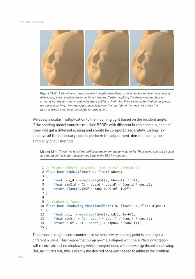
156
We apply a scalar multiplication to the incoming light based on the incident angle. If the shading model contains multiple BSDFs with different bump normals, each of them will get a different scaling and should be computed separately. Listing 12-1 displays all the necessary code to perform the adjustment, demonstrating the simplicity of our method.
Listing 12-1. These two functions suffice to implement the terminator fix. The second one can be used as a multiplier for either the incoming light or the BSDF evaluation.
1 // Return alpha^2 parameter from normal divergence
2 float bump_alpha2(float3 N, float3 Nbump)
3
4 float cos_d = min(fabsf(dot(N, Nbump)), 1.0f);
5 float tan2_d = (1 - cos_d * cos_d) / (cos_d * cos_d);
6 return clamp(0.125f * tan2_d, 0.0f, 1.0f);
7
8
9 // Shadowing factor
10 float bump_shadowing_function(float3 N, float3 Ld, float alpha2)
11
12 float cos_i = max(fabsf(dot(N, Ld)), 1e-6f);
13 float tan2_i = (1 - cos_i * cos_i) / (cos_i * cos_i);
14 return 2.0f / (1 + sqrtf(1 + alpha2 * tan2_i));
15
The proposal might seem counterintuitive since every shading point is due to get a different α value. This means that bump normals aligned with the surface orientation will receive almost no shadowing while divergent ones will receive significant shadowing. But, as it turns out, this is exactly the desired behavior needed to address the problem.
Figure 12-7. Left: when a mesh presents irregular tessellation, the artifacts can become especially distracting, even revealing the underlying triangles. Center: applying the shadowing function as smooths out the terminator and hides these artifacts. Right: but if we try to make shading reciprocal, we unnecessarily darken the edges, especially near the top right of the head. We chose the non-reciprocal version in the middle for production.
RAY TRACING GEMS
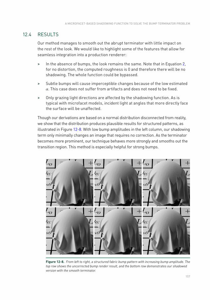
157
12.4 RESULTS
Our method manages to smooth out the abrupt terminator with little impact on the rest of the look. We would like to highlight some of the features that allow for seamless integration into a production renderer:
> In the absence of bumps, the look remains the same. Note that in Equation 2, for no distortion, the computed roughness is 0 and therefore there will be no shadowing. The whole function could be bypassed.
> Subtle bumps will cause imperceptible changes because of the low estimated α. This case does not suffer from artifacts and does not need to be fixed.
> Only grazing light directions are affected by the shadowing function. As is typical with microfacet models, incident light at angles that more directly face the surface will be unaffected.
Though our derivations are based on a normal distribution disconnected from reality, we show that the distribution produces plausible results for structured patterns, as illustrated in Figure 12-8. With low bump amplitudes in the left column, our shadowing term only minimally changes an image that requires no correction. As the terminator becomes more prominent, our technique behaves more strongly and smooths out the transition region. This method is especially helpful for strong bumps.
Figure 12-8. From left to right, a structured fabric bump pattern with increasing bump amplitude. The top row shows the uncorrected bump render result, and the bottom row demonstrates our shadowed version with the smooth terminator.
A MICROFACET-BASED SHADOWING FUNCTION TO SOLVE THE BUMP TERMINATOR PROBLEM
158
ACKNOWLEDGMENTS
This work was developed within the core development of the Arnold renderer at Sony Pictures Imageworks with Christopher Kulla and Larry Gritz.
REFERENCES
[1] Conty Estevez, A., and Lecocq, P. Fast Product Importance Sampling of Environment Maps. In ACM SIGGRAPH 2018 Talks (2018), pp. 69:1–69:2.
[2] Cook, R. L., and Torrance, K. E. A Reflectance Model for Computer Graphics. ACM Transactions on Graphics 1, 1 (Jan. 1982), 7–24.
[3] Dupuy, J., Heitz, E., Iehl, J.-C., Pierre, P., Neyret, F., and Ostromoukhov, V. Linear Efficient Antialiased Displacement and Reflectance Mapping. ACM Transactions on Graphics 32, 6 (Sept. 2013), 211:1–211:11.
[4] Heitz, E. Understanding the Masking-Shadowing Function in Microfacet-Based BRDFs. Journal of Computer Graphics Techniques 3, 2 (June 2014), 48–107.
[5] Max, N. L. Horizon Mapping: Shadows for Bump-Mapped Surfaces. The Visual Computer 4, 2 (Mar 1988), 109–117.
[6] Olano, M., and Baker, D. Lean Mapping. In Symposium on Interactive 3D Graphics and Games (2010), pp. 181–188.
[7] Onoue, K., Max, N., and Nishita, T. Real-Time Rendering of Bumpmap Shadows Taking Account of Surface Curvature. In International Conference on Cyberworlds (Nov 2004), pp. 312–318.
[8] Walter, B., Marschner, S. R., Li, H., and Torrance, K. E. Microfacet Models for Refraction Through Rough Surfaces. In Eurographics Symposium on Rendering (2007), pp. 195–206.
Open Access This chapter is licensed under the terms of the Creative Commons Attribution-NonCommercial-NoDerivatives 4.0 International License (http://creativecommons.org/licenses/by-nc-nd/4.0/), which permits any noncommercial use, sharing, distribution and
reproduction in any medium or format, as long as you give appropriate credit to the original author(s) and the source, provide a link to the Creative Commons license and indicate if you modified the licensed material. You do not have permission under this license to share adapted material derived from this chapter or parts of it.
The images or other third party material in this chapter are included in the chapter's Creative Commons license, unless indicated otherwise in a credit line to the material. If material is not included in the chapter's Creative Commons license and your intended use is not permitted by statutory regulation or exceeds the permitted use, you will need to obtain permission directly from the copyright holder.
RAY TRACING GEMS
159© NVIDIA 2019 E. Haines, T. Akenine-Möller (eds.), Ray Tracing Gems, https://doi.org/10.1007/978-1-4842-4427-2_13
CHAPTER 13
Ray Traced Shadows: Maintaining Real-Time Frame RatesJakub Boksansky,1 Michael Wimmer,2 and Jiri Bittner1
1Czech Technical University in Prague 2Technische Universität Wien
ABSTRACT
Efficient and accurate shadow computation is a long-standing problem in computer graphics. In real-time applications, shadows have traditionally been computed using the rasterization-based pipeline. With recent advances of graphics hardware, it is now possible to use ray tracing in real-time applications, making ray traced shadows a viable alternative to rasterization. While ray traced shadows avoid many problems inherent in rasterized shadows, tracing every shadow ray independently can become a bottleneck if the number of required rays rises, e.g., for high-resolution rendering, for scenes with multiple lights, or for area lights. Therefore, the computation should focus on image regions where shadows actually appear, in particular on the shadow boundaries.
We present a practical method for ray traced shadows in real-time applications. Our method uses the standard rasterization pipeline for resolving primary-ray visibility and ray tracing for resolving visibility of light sources. We propose an adaptive sampling algorithm for shadow rays combined with an adaptive shadow-filtering method. These two techniques allow computing high-quality shadows with a limited number of shadow rays per pixel. We evaluated our method using a recent real-time ray tracing API (DirectX Raytracing) and compare the results with shadow mapping using cascaded shadow maps.
13.1 INTRODUCTION
Shadows contribute significantly to realistic scene perception. Due to the importance of shadows, many techniques have been designed for shadow computation in the past. While offline rendering applications use ray tracing for shadow evaluation [20], real-time applications typically use shadow maps [21]. Shadow mapping is highly flexible in terms of scene geometry, but it has several important issues:
> Perspective aliasing, which shows as jaggy shadows, due to insufficient shadow-map resolution or poor use of its area.
160
> Self-shadowing artifacts (shadow acne) and disconnected shadows (Peter Panning).
> Lack of penumbras (soft shadows).
> Lack of support for semitransparent occluders.
A number of techniques have been developed to address these issues [7, 6]. Usually, a combination of several of them and manual fine-tuning by the scene designer are required to achieve good results. This makes an efficient implementation of shadow mapping complicated, and different solutions are usually required for different scenes.
Ray tracing [20] is a flexible rendering paradigm that can compute accurate shadows with a simple algorithm and is able to handle complex lighting (area lights, semitransparent occluders) in an intuitive and scalable way. However, it has been difficult to achieve ray tracing performance that is sufficient for real-time applications. This was due to limited hardware resources as well as implementation complexity of the underlying algorithms required for real-time ray tracing, such as fast construction and maintenance of spatial data structures. There was also no explicit ray tracing support in popular graphics APIs used for real-time applications.
With the introduction of NVIDIA RTX and DirectX Raytracing (DXR), it is now straightforward to exploit ray tracing using DirectX and Vulkan APIs. The recent NVIDIA Turing graphics architecture provides hardware support for DXR using the dedicated RT Cores, which greatly improve ray tracing performance. These new features combine well with emerging hybrid rendering methods [11] that use rasterization to resolve primary- ray visibility and ray tracing to compute shadows, reflections, and other illuminations effects.
However, even with the new powerful hardware support, we have to use our resources wisely when rendering high-quality shadows using ray tracing. A naive algorithm might easily cast too many rays to sample shadows from multiple light sources and/or area light sources, leading to low frame rates. See Figure 13-1 for an example.
RAY TRACING GEMS
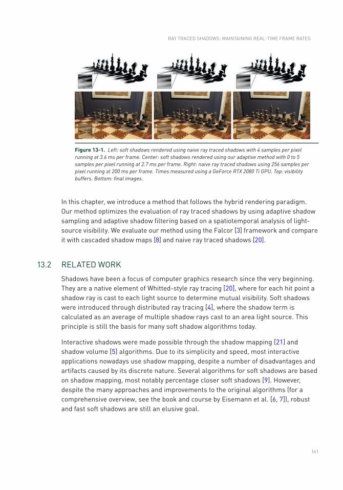
161
In this chapter, we introduce a method that follows the hybrid rendering paradigm. Our method optimizes the evaluation of ray traced shadows by using adaptive shadow sampling and adaptive shadow filtering based on a spatiotemporal analysis of light- source visibility. We evaluate our method using the Falcor [3] framework and compare it with cascaded shadow maps [8] and naive ray traced shadows [20].
13.2 RELATED WORK
Shadows have been a focus of computer graphics research since the very beginning. They are a native element of Whitted-style ray tracing [20], where for each hit point a shadow ray is cast to each light source to determine mutual visibility. Soft shadows were introduced through distributed ray tracing [4], where the shadow term is calculated as an average of multiple shadow rays cast to an area light source. This principle is still the basis for many soft shadow algorithms today.
Interactive shadows were made possible through the shadow mapping [21] and shadow volume [5] algorithms. Due to its simplicity and speed, most interactive applications nowadays use shadow mapping, despite a number of disadvantages and artifacts caused by its discrete nature. Several algorithms for soft shadows are based on shadow mapping, most notably percentage closer soft shadows [9]. However, despite the many approaches and improvements to the original algorithms (for a comprehensive overview, see the book and course by Eisemann et al. [6, 7]), robust and fast soft shadows are still an elusive goal.
Figure 13-1. Left: soft shadows rendered using naive ray traced shadows with 4 samples per pixel running at 3.6 ms per frame. Center: soft shadows rendered using our adaptive method with 0 to 5 samples per pixel running at 2.7 ms per frame. Right: naive ray traced shadows using 256 samples per pixel running at 200 ms per frame. Times measured using a GeForce RTX 2080 Ti GPU. Top: visibility buffers. Bottom: final images.
RAy TRACED SHADOWS: MAINTAININg REAL-TIME FRAME RATES
162
Inspired by advances in interactive ray tracing [18], researchers recently went back to investigating the use of ray tracing for hard and soft shadows. However, instead of performing a full ray tracing pass, a key idea was to use rasterization for the primary rays and to use ray tracing for only shadow rays [1, 19], leading to a hybrid rendering pipeline. To make this viable for soft shadows, the industry is experimenting with temporal accumulation in various ways [2].
The NVIDIA Turing architecture finally introduced fully hardware-accelerated ray tracing to the consumer market, and easy integration with the rasterization pipeline exists in the DirectX (DXR) and Vulkan APIs. Still, soft shadows for multiple light sources pose a challenge and require intelligent adaptive sampling and temporal reprojection approaches, as we will describe in this chapter.
The advent of real-time ray tracing also opens the door for other hybrid rendering techniques, for example adaptive temporal antialiasing, where pixels that cannot be rendered through reprojection are ray traced [14]. Temporal coherence has been used specifically for soft shadows before [17], but here we introduce a much simpler temporal coherence scheme based on a novel variation measure to estimate the required sample count.
13.3 RAy TRACED SHADOWS
Shadows appear when a scene object—a shadow caster—blocks light that would otherwise contribute to illumination at another scene object—the shadow receiver. Shadows can appear due to direct or indirect illumination. Direct illumination shadows are induced when the visibility of primary light sources is blocked, indirect illumination shadows are induced when strong reflections or refractions of light at scene surfaces are blocked. In this chapter, we focus on the case of direct illumination—indirect illumination can be evaluated independently using some standard global-illumination technique such as path tracing or many-light methods.
The outgoing radiance L(p, ωo) at a point P in direction ωo is defined by the rendering equation [12]:
( ) ( ) ( ) ( )( )o e o i o i i i P iL P, L f P, , L P, d ,ˆw w w w w w wòW
= + ×n (1)
where Le(ωo) is the self-emitted radiance, f(P, ωi, ωo) is the BRDF, Li(P, ωi) is the incoming radiance from direction ωi, and nP is the normalized surface normal at point P.
RAY TRACING GEMS
163
For the case of direct illumination with a set of point light sources, the direct illumination component of L can be written as a sum of contributions from individual light sources:
( ) ( ) ( ) ( ) l Pd o l o l l l l
l l
L P, f P, , L P , v P,PP P
2
ˆ,
ww w w w
×=
-å
n (2)
where Pl is the position of light l, the light direction is ωl = (Pl − P)/‖Pl − P‖, Ll(Pl, ωl) is the radiance emitted from light source l in direction ωl, and v(P, Pl) is the visibility term, which equals 1 if the point Pl is visible from P and 0 if it is not.
The evaluation of v(p, pl) can easily be performed by shooting a ray from P toward Pl and checking if the corresponding line segment is unoccluded. Care must be taken near the endpoints of the line segment not to include the self-intersection of the geometry of the shaded point or the light source. This is usually resolved by shrinking the parametric range for valid intersection by a small ε-threshold.
The Ld due to an area light source a is given by
( ) ( ) ( ) ( ) ( )( )X P X Xd o X o a X
X A
L P, f P, , L X , v P, X dAP X
2,
ˆ ˆw ww w w wò
Î
× - ×=
-
n n (3)
where A is the surface of light a, nX is the normal of the light source surface at point X, ωX = (X − P)/‖X − P‖ is the direction from point P toward point X on the light source, La(X, ωX) is the radiance emitted from point X in direction ωX, and v(P, X) is the visibility term that equals 1 if the point X is visible from P and 0 if it is not.
This integral is commonly evaluated by Monte Carlo integration using a set of well- distributed samples S on the light source:
( ) ( ) ( ) ( ) ( )( )X P X Xd o X o a X
X S
L P, f P, , L X , v P, XS P X
2
ˆ ˆ1 ,w w
w w w wÎ
× - ×»
-å
n n
∣∣ (4)
where ∣ S∣ is the number of light samples. In our work we separate the shading and visibility terms, and for shading we approximate the area light source with a centroid C of the light source:
( ) ( ) ( ) ( )( ) ( )C P C Cd o C o a C
X S
L P, f P, , L C, v P, XSP C
2
ˆ ˆ 1 .w w
w w w wÎ
× - ×»
-å
n n
∣∣ (5)
This allows us to accumulate the results of visibility tests for each light within a given frame and store them in a dedicated visibility buffer for each light. The visibility buffer is a screen-sized texture that holds visibility terms for each pixel. A more elaborate
RAy TRACED SHADOWS: MAINTAININg REAL-TIME FRAME RATES
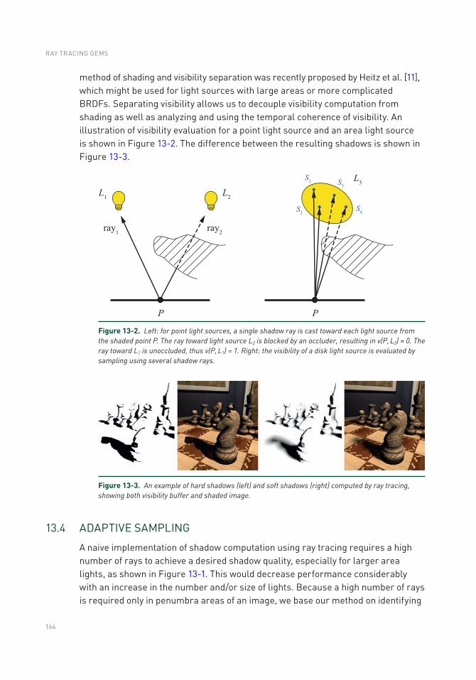
164
method of shading and visibility separation was recently proposed by Heitz et al. [11], which might be used for light sources with large areas or more complicated BRDFs. Separating visibility allows us to decouple visibility computation from shading as well as analyzing and using the temporal coherence of visibility. An illustration of visibility evaluation for a point light source and an area light source is shown in Figure 13-2. The difference between the resulting shadows is shown in Figure 13-3.
Figure 13-2. Left: for point light sources, a single shadow ray is cast toward each light source from the shaded point P. The ray toward light source L2 is blocked by an occluder, resulting in v(P, L2) = 0. The ray toward L1 is unoccluded, thus v(P, L1) = 1. Right: the visibility of a disk light source is evaluated by sampling using several shadow rays.
Figure 13-3. An example of hard shadows (left) and soft shadows (right) computed by ray tracing, showing both visibility buffer and shaded image.
13.4 ADAPTIVE SAMPLINg
A naive implementation of shadow computation using ray tracing requires a high number of rays to achieve a desired shadow quality, especially for larger area lights, as shown in Figure 13-1. This would decrease performance considerably with an increase in the number and/or size of lights. Because a high number of rays is required only in penumbra areas of an image, we base our method on identifying
RAY TRACING GEMS
165
these areas and then using more rays to sample them effectively. The fully lit and fully occluded areas are sampled sparsely, and the saved computational resources can be used for other ray tracing tasks such as reflections.
13.4.1 TEMPORAL REPROJECTION
To effectively increase the sample count used per pixel, we use temporal reprojection, which allows us to accumulate visibility values for visible scene surfaces over time. Temporal reprojection is becoming a standard tool in many recent real-time rendering methods [15], and in many cases it is already implemented within the application rasterization pipeline. We use the accumulated values for two purposes: first, estimating visibility variation to derive the required sample count, and second, determining the kernel size for filtering the sampled visibility.
We store the results of visibility calculations from previous frames in a cache containing four frames. To ensure correct results for dynamic scenes, we use reverse reprojection [15], which handles the camera movement. When starting an evaluation of a new frame, we perform reverse reprojection of three previous frames, stored in the cache, to the current frame. Thus, we always have a four-tuple of values from four consequent frames aligned with the image corresponding to the current frame.
given a point Pt in clip space in frame t, the reprojection finds the corresponding clip-space coordinates
tP 1- in frame t − 1 as
t t t t t tP P1 11 1 1 ,- -
- - -= C V V C (6)
where Ct and Ct − 1 are the camera projection matrices and Vt and Vt − 1 are the camera viewing matrices. After reprojection we check for depth discontinuities and discard invalid correspondences (mostly disocclusions). Depth discontinuities are detected using a relative depth difference condition, i.e., the point is successfully reprojected if the following condition holds:
z
tzz
t
Pc c n
P1
1 21
1 , ˆ ,e e-
-
- < = + (7)
where ε is an adaptive depth similarity threshold, zn is a z-coordinate of the view- space normal of the corresponding pixel, and c1 and c2 are user-specified constants of linear interpolation (we used c1 = 0.003 and c2 = 0.017). The adaptive threshold ε allows for greater depth differences of valid samples on sloped surfaces.
RAy TRACED SHADOWS: MAINTAININg REAL-TIME FRAME RATES
166
For successfully reprojected points, we store image-space coordinates in the range 0 to 1. If the reprojection fails, we store negative values to indicate the reprojection failure for subsequent computations. Note that, as all previous frames have already been aligned during the previous reprojection steps, only one cache entry for storing the depth values z
tP 1- is sufficient.
13.4.2 IDENTIFyINg PENUMBRA REgIONS
The number of samples (rays) required for a given combination of shaded point and light source generally depends on the light size, its distance to the shaded point, and the complexity of occluding geometry. Because this complexity would be difficult to analyze, we base our method on using the temporal visibility variation measure Δv(x):
( ) ( ) ( )( ) ( ) ( )( )t t t t tv x v x v x v x v x1 4 1 4max min ,- - - -D = ¼ - ¼ (8)
where vt − 1(x) … vt − 4(x) are the cached visibility values for a pixel x in the four previous frames. Note that these visibility values are cached in a single four-component texture per light.
The described measure corresponds to the range variation measure, which is highly sensitive to extreme values of the visibility function. Therefore, this measure is more likely to detect penumbra regions than other, smoother variation measures such as the variance.
The variation is zero for either fully lit or fully occluded areas and is usually greater than zero in penumbra areas. Our sample sets are generated with regard to the fact that we use four frames for variation computation, so they repeat only after these four frames. See Section 13.5.1.
To make results more temporally stable, we apply a spatial filter on the variation measure followed by a temporal filter. The spatial filter is expressed as
( )t tv M v T5 5 13 13,´ ´D = D * (9)
where M5 × 5 is a nonlinear maximum filter using a 5 × 5 neighborhood followed by a convolution with a low-pass tent filter T13 × 13 with a 13 × 13 neighborhood. The maximum filter makes sure that a high variation detected in a single pixel will cause a higher number of samples to be used in surrounding pixels too. This is important for dynamic scenes to make the method more temporally stable and for cases where the penumbra is completely missed in nearby pixels. The tent
RAY TRACING GEMS
167
filter prevents abrupt changes in variation values to avoid flickering. Both filters are separable, therefore we execute them in two passes to reduce the computational effort.
Finally, we combine the spatially filtered variation measure tvD with temporally filtered values Δvt from the four previous frames. For the temporal filtering, we use a simple box filter, and we intentionally use the raw Δvt values that are cached prior to spatial filtering:
( )t t t t t tv v v v v v1 2 3 4
1 1 .2 4 - - - -
æ öD = D + D + D + D + Dç ÷
è ø (10)
Such a combination of filters proved efficient in our tests as it is able to propagate the variation over larger regions (using maximum and tent filters). At the same time, it does not miss small regions with large variation by combining the spatially filtered variation with the temporally filtered variation values from the previous frames.
13.4.3 COMPUTINg THE NUMBER OF SAMPLES
The decision on the number of samples to be used for a given point is based on the number of samples used in the previous frame and the current filtered variation tvD . We use a threshold δ on the variation measure to decide whether to increase or decrease sampling density at the corresponding pixel. In particular, we maintain the sample counts s(x) for each pixel and use the following algorithm to update s(x) in the given frame:
1. If ( )tv x dD > and st − 1(x) < smax, increase the number of samples by one (st(x) = st − 1(x) + 1).
2. If ( )tv x dD < and the number of samples has been stable in the four previous frames, decrease the number of samples (st(x) = st − 1(x) − 1).
The maximum number of samples per light smax ensures a limited ray budget for each light per frame (we use smax = 5 for standard settings and smax = 8 for high-quality settings). The constraint of stability in the four previous frames used in step (2) induces a hysteresis into the algorithm and aims to prevent oscillations in the number of samples caused by a feedback loop between the number of samples and the variation. The described technique works with sufficient temporal stability and provides better results than directly computing s(x) from ( )tv xD .
RAy TRACED SHADOWS: MAINTAININg REAL-TIME FRAME RATES
168
For pixels where reverse reprojection fails, we use smax samples and replace all cached visibility values with the current result. When a reverse reprojection fails for all pixels on the screen, e.g., when the camera pose changes dramatically, a sudden performance drop occurs due to the high number of samples used in each pixel. To prevent the performance drop, we can detect large changes of camera pose on the CPU, and we can reduce the maximum number of samples (smax) for several subsequent frames. This will momentarily cause noisier results, but it will prevent frame-rate stuttering, which is usually more disturbing.
13.4.4 SAMPLINg MASK
Pixels for which our algorithm computes sample counts equal to zero indicate a region with no temporal and spatial variation. This is mostly the case for fully lit and fully shadowed regions in an image. For these pixels we might skip the calculation of visibility completely and use value from the previous frame. However, this may lead to an accumulation of errors over time in these regions, for example when a light is moving fast or the camera is zooming slowly (in both these cases the reprojection succeeds, but visibility can change). Therefore, we use a mask that enforces regular sampling for at least one fourth of the pixels. We enforce sampling of individual blocks of pixels on the screen as performance tests have shown that shooting a single ray for one pixel out of four in a close neighborhood yields similar performance as shooting rays for each of these pixels (probably due to warp dependencies). Therefore, we enforce sampling of a block of nb × nb pixels on the screen (we get the best performance increase for nb = 8).
To ensure that every pixel is sampled at least once in four frames, we use a matrix that checks if the sampling should be enforced in the current frame. We find an entry in a mask of size 4 × 4 repeated over the screen that corresponds to the location of the block. If the entry is equal to the current frame’s sequence number modulo four, all pixels in blocks with zero sample counts are sampled with one shadow ray per pixel per light. The mask is set up so that in each quad of neighboring blocks, only one block will be evaluated. Furthermore, every pixel will be evaluated once in four consecutive frames to make sure that new shadows are detected. This is illustrated in Figure 13-4. An example of the sample distribution using the adaptive sampling is shown in Figure 13-5.
RAY TRACING GEMS
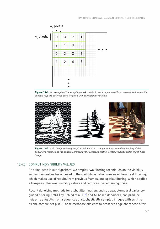
169
13.4.5 COMPUTINg VISIBILITy VALUES
As a final step in our algorithm, we employ two filtering techniques on the visibility values themselves (as opposed to the visibility variation measure): temporal filtering, which makes use of results from previous frames, and spatial filtering, which applies a low-pass filter over visibility values and removes the remaining noise.
Recent denoising methods for global illumination, such as spatiotemporal variance- guided filtering (SVgF) by Schied et al. [16] and AI-based denoisers, can produce noise-free results from sequences of stochastically sampled images with as little as one sample per pixel. These methods take care to preserve edge sharpness after
Figure 13-4. An example of the sampling mask matrix. In each sequence of four consecutive frames, the shadow rays are enforced even for pixels with low visibility variation.
Figure 13-5. Left: image showing the pixels with nonzero sample counts. Note the sampling of the penumbra regions and the pattern enforced by the sampling matrix. Center: visibility buffer. Right: final image.
RAy TRACED SHADOWS: MAINTAININg REAL-TIME FRAME RATES
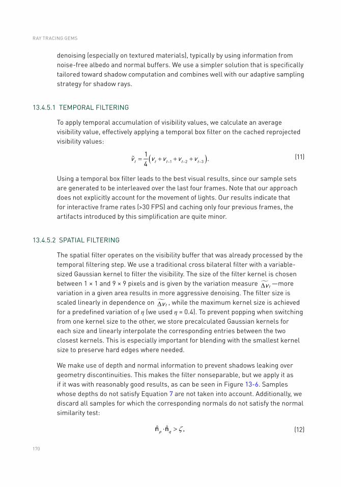
170
denoising (especially on textured materials), typically by using information from noise-free albedo and normal buffers. We use a simpler solution that is specifically tailored toward shadow computation and combines well with our adaptive sampling strategy for shadow rays.
13.4.5.1 TEMPORAL FILTERINg
To apply temporal accumulation of visibility values, we calculate an average visibility value, effectively applying a temporal box filter on the cached reprojected visibility values:
( )t t t t tv vv v v1 2 3
1 .4 - - -= + + + (11)
Using a temporal box filter leads to the best visual results, since our sample sets are generated to be interleaved over the last four frames. Note that our approach does not explicitly account for the movement of lights. Our results indicate that for interactive frame rates (>30 FPS) and caching only four previous frames, the artifacts introduced by this simplification are quite minor.
13.4.5.2 SPATIAL FILTERINg
The spatial filter operates on the visibility buffer that was already processed by the temporal filtering step. We use a traditional cross bilateral filter with a variable-sized gaussian kernel to filter the visibility. The size of the filter kernel is chosen between 1 × 1 and 9 × 9 pixels and is given by the variation measure tvD —more variation in a given area results in more aggressive denoising. The filter size is scaled linearly in dependence on tvD , while the maximum kernel size is achieved for a predefined variation of η (we used η = 0.4). To prevent popping when switching from one kernel size to the other, we store precalculated gaussian kernels for each size and linearly interpolate the corresponding entries between the two closest kernels. This is especially important for blending with the smallest kernel size to preserve hard edges where needed.
We make use of depth and normal information to prevent shadows leaking over geometry discontinuities. This makes the filter nonseparable, but we apply it as if it was with reasonably good results, as can be seen in Figure 13-6. Samples whose depths do not satisfy Equation 7 are not taken into account. Additionally, we discard all samples for which the corresponding normals do not satisfy the normal similarity test:
p qˆ ˆ ,z× >n n (12)
RAY TRACING GEMS
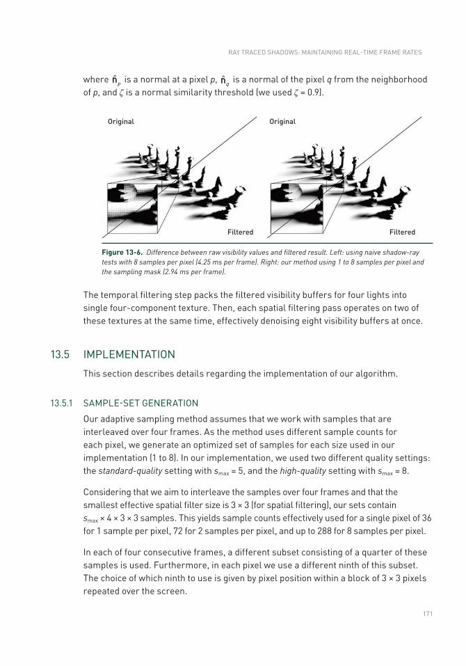
171
where pn is a normal at a pixel p, qn is a normal of the pixel q from the neighborhood of p, and ζ is a normal similarity threshold (we used ζ = 0.9).
Figure 13-6. Difference between raw visibility values and filtered result. Left: using naive shadow-ray tests with 8 samples per pixel (4.25 ms per frame). Right: our method using 1 to 8 samples per pixel and the sampling mask (2.94 ms per frame).
The temporal filtering step packs the filtered visibility buffers for four lights into single four-component texture. Then, each spatial filtering pass operates on two of these textures at the same time, effectively denoising eight visibility buffers at once.
13.5 IMPLEMENTATION
This section describes details regarding the implementation of our algorithm.
13.5.1 SAMPLE-SET gENERATION
Our adaptive sampling method assumes that we work with samples that are interleaved over four frames. As the method uses different sample counts for each pixel, we generate an optimized set of samples for each size used in our implementation (1 to 8). In our implementation, we used two different quality settings: the standard-quality setting with smax = 5, and the high-quality setting with smax = 8.
Considering that we aim to interleave the samples over four frames and that the smallest effective spatial filter size is 3 × 3 (for spatial filtering), our sets contain smax × 4 × 3 × 3 samples. This yields sample counts effectively used for a single pixel of 36 for 1 sample per pixel, 72 for 2 samples per pixel, and up to 288 for 8 samples per pixel.
In each of four consecutive frames, a different subset consisting of a quarter of these samples is used. Furthermore, in each pixel we use a different ninth of this subset. The choice of which ninth to use is given by pixel position within a block of 3 × 3 pixels repeated over the screen.
RAy TRACED SHADOWS: MAINTAININg REAL-TIME FRAME RATES
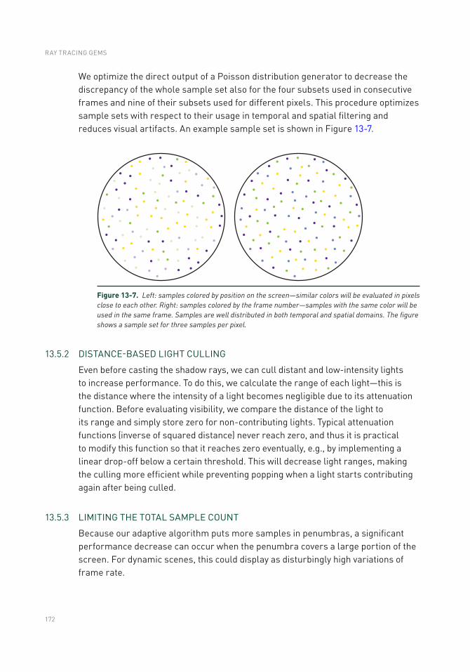
172
We optimize the direct output of a Poisson distribution generator to decrease the discrepancy of the whole sample set also for the four subsets used in consecutive frames and nine of their subsets used for different pixels. This procedure optimizes sample sets with respect to their usage in temporal and spatial filtering and reduces visual artifacts. An example sample set is shown in Figure 13-7.
13.5.2 DISTANCE-BASED LIgHT CULLINg
Even before casting the shadow rays, we can cull distant and low-intensity lights to increase performance. To do this, we calculate the range of each light—this is the distance where the intensity of a light becomes negligible due to its attenuation function. Before evaluating visibility, we compare the distance of the light to its range and simply store zero for non-contributing lights. Typical attenuation functions (inverse of squared distance) never reach zero, and thus it is practical to modify this function so that it reaches zero eventually, e.g., by implementing a linear drop-off below a certain threshold. This will decrease light ranges, making the culling more efficient while preventing popping when a light starts contributing again after being culled.
13.5.3 LIMITINg THE TOTAL SAMPLE COUNT
Because our adaptive algorithm puts more samples in penumbras, a significant performance decrease can occur when the penumbra covers a large portion of the screen. For dynamic scenes, this could display as disturbingly high variations of frame rate.
Figure 13-7. Left: samples colored by position on the screen—similar colors will be evaluated in pixels close to each other. Right: samples colored by the frame number—samples with the same color will be used in the same frame. Samples are well distributed in both temporal and spatial domains. The figure shows a sample set for three samples per pixel.
RAY TRACING GEMS
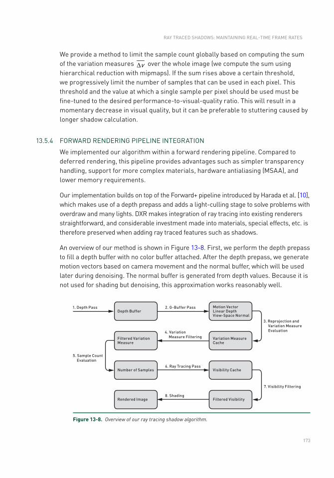
173
We provide a method to limit the sample count globally based on computing the sum of the variation measures vD over the whole image (we compute the sum using hierarchical reduction with mipmaps). If the sum rises above a certain threshold, we progressively limit the number of samples that can be used in each pixel. This threshold and the value at which a single sample per pixel should be used must be fine-tuned to the desired performance-to-visual-quality ratio. This will result in a momentary decrease in visual quality, but it can be preferable to stuttering caused by longer shadow calculation.
13.5.4 FORWARD RENDERINg PIPELINE INTEgRATION
We implemented our algorithm within a forward rendering pipeline. Compared to deferred rendering, this pipeline provides advantages such as simpler transparency handling, support for more complex materials, hardware antialiasing (MSAA), and lower memory requirements.
Our implementation builds on top of the Forward+ pipeline introduced by Harada et al. [10], which makes use of a depth prepass and adds a light-culling stage to solve problems with overdraw and many lights. DXR makes integration of ray tracing into existing renderers straightforward, and considerable investment made into materials, special effects, etc. is therefore preserved when adding ray traced features such as shadows.
An overview of our method is shown in Figure 13-8. First, we perform the depth prepass to fill a depth buffer with no color buffer attached. After the depth prepass, we generate motion vectors based on camera movement and the normal buffer, which will be used later during denoising. The normal buffer is generated from depth values. Because it is not used for shading but denoising, this approximation works reasonably well.
Figure 13-8. Overview of our ray tracing shadow algorithm.
RAy TRACED SHADOWS: MAINTAININg REAL-TIME FRAME RATES
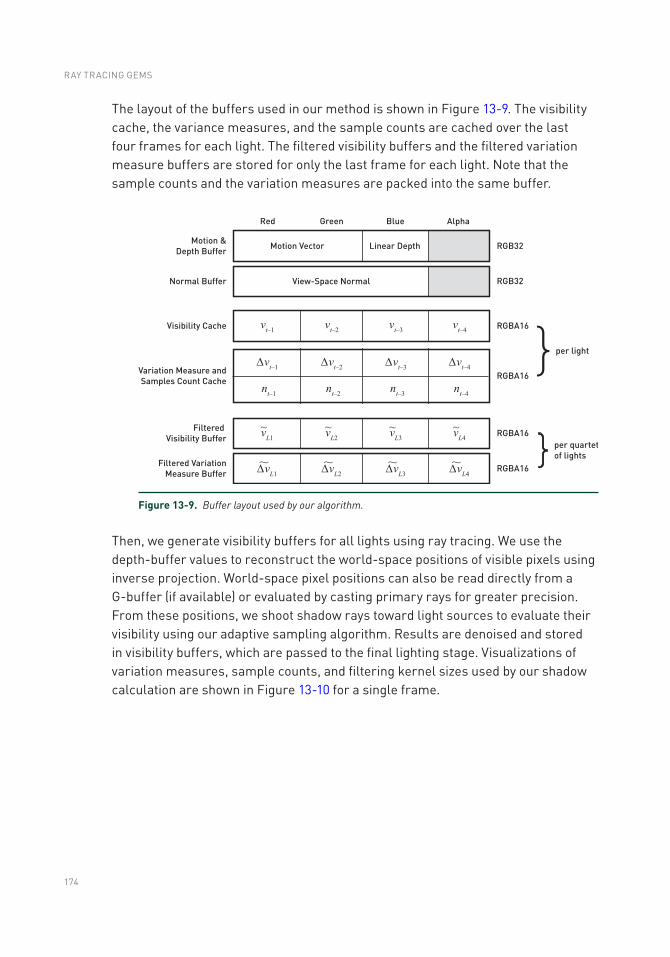
174
The layout of the buffers used in our method is shown in Figure 13-9. The visibility cache, the variance measures, and the sample counts are cached over the last four frames for each light. The filtered visibility buffers and the filtered variation measure buffers are stored for only the last frame for each light. Note that the sample counts and the variation measures are packed into the same buffer.
Then, we generate visibility buffers for all lights using ray tracing. We use the depth- buffer values to reconstruct the world-space positions of visible pixels using inverse projection. World-space pixel positions can also be read directly from a g-buffer (if available) or evaluated by casting primary rays for greater precision. From these positions, we shoot shadow rays toward light sources to evaluate their visibility using our adaptive sampling algorithm. Results are denoised and stored in visibility buffers, which are passed to the final lighting stage. Visualizations of variation measures, sample counts, and filtering kernel sizes used by our shadow calculation are shown in Figure 13- 10 for a single frame.
Figure 13-9. Buffer layout used by our algorithm.
RAY TRACING GEMS
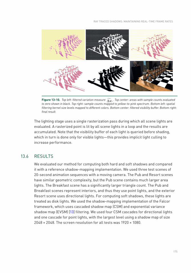
175
The lighting stage uses a single rasterization pass during which all scene lights are evaluated. A rasterized point is lit by all scene lights in a loop and the results are accumulated. Note that the visibility buffer of each light is queried before shading, which in turn is done only for visible lights—this provides implicit light culling to increase performance.
13.6 RESULTS
We evaluated our method for computing both hard and soft shadows and compared it with a reference shadow-mapping implementation. We used three test scenes of 20-second animation sequences with a moving camera. The Pub and Resort scenes have similar geometric complexity, but the Pub scene contains much larger area lights. The Breakfast scene has a significantly larger triangle count. The Pub and Breakfast scenes represent interiors, and thus they use point lights, and the exterior Resort scene uses directional lights. For computing soft shadows, these lights are treated as disk lights. We used the shadow-mapping implementation of the Falcor framework, which uses cascaded shadow map (CSM) and exponential variance shadow map (EVSM) [13] filtering. We used four CSM cascades for directional lights and one cascade for point lights, with the largest level using a shadow map of size 2048 × 2048. The screen resolution for all tests was 1920 × 1080.
Figure 13-10. Top left: filtered variation measure tvD . Top center: areas with sample counts evaluated to zero shown in black. Top right: sample counts mapped to yellow-to-pink spectrum. Bottom left: spatial filtering kernel size levels mapped to different colors. Bottom center: filtered visibility buffer. Bottom right: final result.
RAy TRACED SHADOWS: MAINTAININg REAL-TIME FRAME RATES
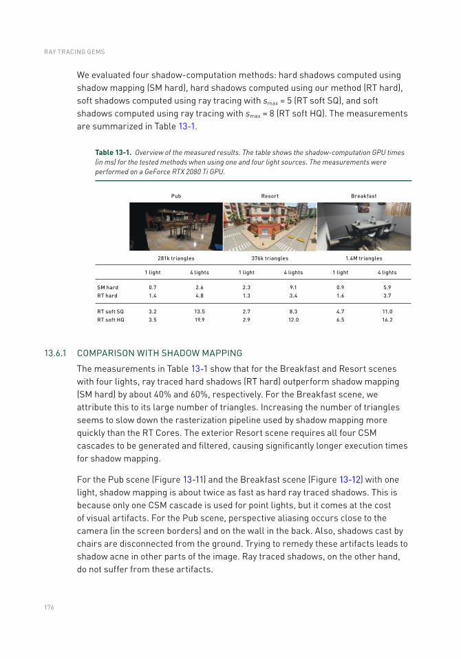
176
We evaluated four shadow-computation methods: hard shadows computed using shadow mapping (SM hard), hard shadows computed using our method (RT hard), soft shadows computed using ray tracing with smax = 5 (RT soft SQ), and soft shadows computed using ray tracing with smax = 8 (RT soft HQ). The measurements are summarized in Table 13-1.
Table 13-1. Overview of the measured results. The table shows the shadow- computation GPU times (in ms) for the tested methods when using one and four light sources. The measurements were performed on a GeForce RTX 2080 Ti GPU.
13.6.1 COMPARISON WITH SHADOW MAPPINg
The measurements in Table 13-1 show that for the Breakfast and Resort scenes with four lights, ray traced hard shadows (RT hard) outperform shadow mapping (SM hard) by about 40% and 60%, respectively. For the Breakfast scene, we attribute this to its large number of triangles. Increasing the number of triangles seems to slow down the rasterization pipeline used by shadow mapping more quickly than the RT Cores. The exterior Resort scene requires all four CSM cascades to be generated and filtered, causing significantly longer execution times for shadow mapping.
For the Pub scene (Figure 13-11) and the Breakfast scene (Figure 13-12) with one light, shadow mapping is about twice as fast as hard ray traced shadows. This is because only one CSM cascade is used for point lights, but it comes at the cost of visual artifacts. For the Pub scene, perspective aliasing occurs close to the camera (in the screen borders) and on the wall in the back. Also, shadows cast by chairs are disconnected from the ground. Trying to remedy these artifacts leads to shadow acne in other parts of the image. Ray traced shadows, on the other hand, do not suffer from these artifacts.
RAY TRACING GEMS
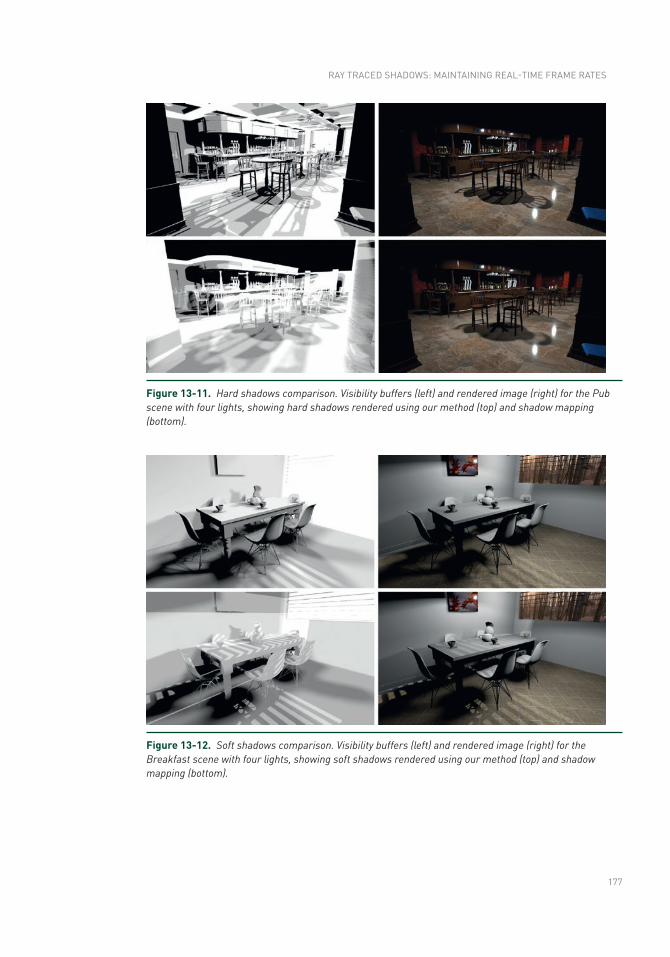
177
Figure 13-11. Hard shadows comparison. Visibility buffers (left) and rendered image (right) for the Pub scene with four lights, showing hard shadows rendered using our method (top) and shadow mapping (bottom).
Figure 13-12. Soft shadows comparison. Visibility buffers (left) and rendered image (right) for the Breakfast scene with four lights, showing soft shadows rendered using our method (top) and shadow mapping (bottom).
RAy TRACED SHADOWS: MAINTAININg REAL-TIME FRAME RATES
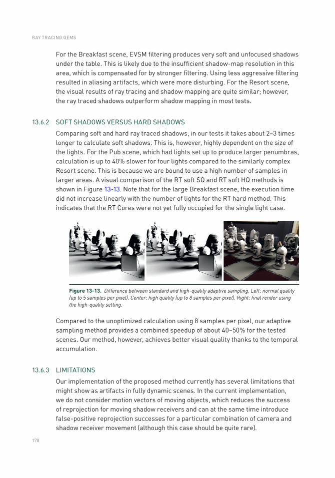
178
For the Breakfast scene, EVSM filtering produces very soft and unfocused shadows under the table. This is likely due to the insufficient shadow-map resolution in this area, which is compensated for by stronger filtering. Using less aggressive filtering resulted in aliasing artifacts, which were more disturbing. For the Resort scene, the visual results of ray tracing and shadow mapping are quite similar; however, the ray traced shadows outperform shadow mapping in most tests.
13.6.2 SOFT SHADOWS VERSUS HARD SHADOWS
Comparing soft and hard ray traced shadows, in our tests it takes about 2–3 times longer to calculate soft shadows. This is, however, highly dependent on the size of the lights. For the Pub scene, which had lights set up to produce larger penumbras, calculation is up to 40% slower for four lights compared to the similarly complex Resort scene. This is because we are bound to use a high number of samples in larger areas. A visual comparison of the RT soft SQ and RT soft HQ methods is shown in Figure 13-13. Note that for the large Breakfast scene, the execution time did not increase linearly with the number of lights for the RT hard method. This indicates that the RT Cores were not yet fully occupied for the single light case.
Compared to the unoptimized calculation using 8 samples per pixel, our adaptive sampling method provides a combined speedup of about 40–50% for the tested scenes. Our method, however, achieves better visual quality thanks to the temporal accumulation.
13.6.3 LIMITATIONS
Our implementation of the proposed method currently has several limitations that might show as artifacts in fully dynamic scenes. In the current implementation, we do not consider motion vectors of moving objects, which reduces the success of reprojection for moving shadow receivers and can at the same time introduce false-positive reprojection successes for a particular combination of camera and shadow receiver movement (although this case should be quite rare).
Figure 13-13. Difference between standard and high-quality adaptive sampling. Left: normal quality (up to 5 samples per pixel). Center: high quality (up to 8 samples per pixel). Right: final render using the high-quality setting.
RAY TRACING GEMS
179
More significantly, moving shadow casters are not handled by the method, which might introduce temporal shadow artifacts. On the positive side, our method uses a limited-size temporal buffer (only the last four frames are considered), and in combination with the aggressive variability measure, it will usually enforce dense sampling of the dynamic penumbras. Another problematic case is moving light sources, which we do not address explicitly at the moment. The situation is similar to moving shadow casters: a quickly moving light source causes severe changes in shadows that reduce the potential of adaptive sampling and can cause ghosting artifacts.
The current algorithm for maintaining a per-frame ray budget is relatively simple, and it would be desirable to use a technique that would directly relate the variation measure to the number of samples while aiming to minimize the perceived error (including shading). In that case it would be easier to guarantee frame rates while obtaining shadows of highest possible quality.
13.7 CONCLUSION AND FUTURE WORK
In this chapter, we have presented a method for calculating ray traced shadows using the modern DXR API within a rasterization forward-rendering pipeline. We proposed an adaptive shadow-sampling method that is based on estimating the variation of the visibility function over surfaces seen by the camera. Our method produces hard shadows as well as soft shadows using lights of various sizes. We have evaluated various configurations of light-sampling and shadow-filtering techniques and provided recommendations for best results.
We compared our method to a state-of-the-art shadow-mapping implementation in terms of visual quality and performance. In general, we conclude that the higher visual quality, simpler implementation, and high performance of ray traced shadows makes them preferable over shadow mapping on DXR-capable hardware. This will also move the burden of calculating shadows from rasterization to ray tracing hardware units, making more performance available for rasterization tasks. Using AI-based denoisers running on dedicated gPU cores can help even more in this respect.
With shadow mapping, scene designers are often challenged with minimizing the technique’s artifacts by setting up technical parameters such as near/far planes, shadow- map resolutions, and bias and penumbra sizes not related to physical lighting. With ray traced shadows, there is still a burden on designers to make shadow calculation efficient and noise-free by using reasonable light sizes, ranges, and placement. We believe, however, that these parameters are more intuitive and closer to physically based lighting.
RAy TRACED SHADOWS: MAINTAININg REAL-TIME FRAME RATES
180
13.7.1 FUTURE WORK
Our method does not explicitly handle movement of lights, which can lead to ghosting artifacts from rapid light movement. A correct approach would be to discard cached visibility from previous frames when it is no longer valid after light movement between the frames.
Shadow mapping is not view-dependent, and a common optimization is to calculate shadow maps only when either a light or the scene changes. This optimization is not applicable for ray tracing, as ray traced visibility buffers need to be recalculated after every camera movement. Because of this, shadow mapping can still be preferable for scenarios where the shadow map is rarely updated. Therefore, a combination of high- quality ray traced shadows for significant light sources and shadow mapping for mostly static parts of the scene and/or less contributing lights can be desirable.
As mentioned in Section 13.3, an improved approach to combining shadows evaluated using our method with the analytic direct illumination, such as the one introduced by Heitz et al. [11], can be used to improve the correctness of the rendered images.
ACKNOWLEDgEMENTS
We thank Tomas Akenine-Möller for his feedback and help with the performance measurements, Nir Benty for assistance with the Falcor framework, and David Sedlacek for providing the environment maps. This research was supported by the Czech Science Foundation under project number gA18-20374S and by the MŠMT under the identification code 7AMB17AT021 within the activity MOBILITy (MSMT-539/2017-1).
REFERENCES
[1] Anagnostou, K. Hybrid Ray Traced Shadows and Reflections. Interplay of Light Blog, https://interplayoflight.wordpress.com/2018/07/04/hybrid-raytraced-shadows-and-
reflections/, July 2018.
[2] Barré-Brisebois, Colin. Halén, H. PICA PICA & NVIDIA Turing. Real-Time Ray Tracing Sponsored Session, SIggRAPH, 2018.
[3] Benty, N., yao, K.-H., Foley, T., Kaplanyan, A. S., Lavelle, C., Wyman, C., and Vijay, A. The Falcor Rendering Framework. https://github.com/NVIDIAGameWorks/Falcor, July 2017.
[4] Cook, R. L., Porter, T., and Carpenter, L. Distributed Ray Tracing. Computer Graphics (SIGGRAPH) 18, 3 (July 1984), 137–145.
RAY TRACING GEMS
181
[5] Crow, F. C. Shadow Algorithms for Computer graphics. Computer Graphics (SIGGRAPH) 11, 2 (August 1977), 242–248.
[6] Eisemann, E., Assarsson, U., Schwarz, M., Valient, M., and Wimmer, M. Efficient Real-Time Shadows. In ACM SIGGRAPH Courses (2013), pp. 18:1–18:54.
[7] Eisemann, E., Schwarz, M., Assarsson, U., and Wimmer, M. Real-Time Shadows, first ed. A K Peters Ltd., 2011.
[8] Engel, W. Cascaded Shadow Maps. In ShaderX5: Advanced Rendering Techniques, W. Engel, Ed. Charles River Media, 2006, pp. 197–206.
[9] Fernando, R. Percentage-Closer Soft Shadows. In ACM SIGGRAPH Sketches and Applications (July 2005), p. 35.
[10] Harada, T., McKee, J., and yang, J. C. Forward+: Bringing Deferred Lighting to the Next Level. In Eurographics Short Papers (2012), pp. 5–8.
[11] Heitz, E., Hill, S., and Mcguire, M. Combining Analytic Direct Illumination and Stochastic Shadows. In Symposium on Interactive 3D Graphics and Games (2018), pp. 2:1–2:11.
[12] Kajiya, J. T. The Rendering Equation. Computer Graphics (SIGGRAPH) 20, 4 (August 1986), 143–150.
[13] Lauritzen, A. T. Rendering Antialiased Shadows using Warped Variance Shadow Maps. Master’s thesis, University of Waterloo, 2008.
[14] Marrs, A., Spjut, J., gruen, H., Sathe, R., and Mcguire, M. Adaptive Temporal Antialiasing. In Proceedings of High-Performance Graphics (2018), pp. 1:1–1:4.
[15] Scherzer, D., yang, L., Mattausch, O., Nehab, D., Sander, P. V., Wimmer, M., and Eisemann, E. A Survey on Temporal Coherence Methods in Real-Time Rendering. In Eurographics State of the Art Reports (2011), pp. 101–126.
[16] Schied, C., Kaplanyan, A., Wyman, C., Patney, A., Chaitanya, C. R. A., Burgess, J., Liu, S., Dachsbacher, C., Lefohn, A., and Salvi, M. Spatiotemporal Variance- guided Filtering: Real-Time Reconstruction for Path-Traced global Illumination. In Proceedings of High-Performance Graphics (2017), pp. 2:1–2:12.
[17] Schwärzler, M., Luksch, C., Scherzer, D., and Wimmer, M. Fast Percentage Closer Soft Shadows Using Temporal Coherence. In Symposium on Interactive 3D Graphics and Games (March 2013), pp. 79–86.
[18] Shirley, P., and Slusallek, P. State of the Art in Interactive Ray Tracing. ACM SIggRAPH Courses, 2006.
[19] Story, J. Hybrid Ray Traced Shadows, https://developer.nvidia.com/content/hybrid-ray-traced-shadows. NVIDIA gameworks Blog, June 2015.
[20] Whitted, T. An Improved Illumination Model for Shaded Display. Communications of the ACM 23, 6 (June 1980), 343–349.
[21] Williams, L. Casting Curved Shadows on Curved Surfaces. Computer Graphics SIGGRAPH() 12, 3 (August 1978), 270–274.
RAy TRACED SHADOWS: MAINTAININg REAL-TIME FRAME RATES

182
Open Access This chapter is licensed under the terms of the Creative Commons Attribution-NonCommercial-NoDerivatives 4.0 International License (http://creativecommons.org/licenses/by-nc-nd/4.0/), which permits any noncommercial use, sharing, distribution and
reproduction in any medium or format, as long as you give appropriate credit to the original author(s) and the source, provide a link to the Creative Commons license and indicate if you modified the licensed material. you do not have permission under this license to share adapted material derived from this chapter or parts of it.
The images or other third party material in this chapter are included in the chapter's Creative Commons license, unless indicated otherwise in a credit line to the material. If material is not included in the chapter's Creative Commons license and your intended use is not permitted by statutory regulation or exceeds the permitted use, you will need to obtain permission directly from the copyright holder.
RAY TRACING GEMS
183© NVIDIA 2019 E. Haines, T. Akenine-Möller (eds.), Ray Tracing Gems, https://doi.org/10.1007/978-1-4842-4427-2_14
CHAPTER 14
Ray-Guided Volumetric Water Caustics in Single Scattering Media with DXRHolger Gruen NVIDIA
ABSTRACT
This chapter presents a hybrid algorithm that uses ray tracing and rasterization to render surface and volumetric caustics in single scattering participating media. The algorithm makes use of ray tracing based on DirectX Raytracing (DXR) to generate data that drives hardware tessellation to adaptively refine triangular beam volumes that are rendered to slice volumetric caustics. Further on in the rendering pipeline, ray tracing is also used to generate secondary caustics maps that store the positions of ray/scene intersections for light rays that get reflected or refracted by a water surface.
14.1 INTRODUCTION
This chapter investigates how to make use of the DirectX 12 real-time ray tracing API, DXR, to simplify current methods for rendering real-time volumetric water caustics in single scattering media. Volumetric caustics have been investigated extensively in the past [2, 5, 6, 10]. The algorithm described here uses ideas discussed in the literature and combines them with the use of DXR ray tracing and adaptive hardware tessellation.
Specifically, for rendering volumetric caustics, ray tracing is used twice in the rendering pipeline. In an initial step, ray tracing is used to compute information that then guides hardware tessellation levels for triangular beam volumes that are used to adaptively slice caustics volumes. The rendering pipeline for accumulating volumetric light that is scattered toward the eye uses all GPU shader stages, e.g., a vertex shader, a hull shader, a domain shader, a geometry shader, and a pixel shader.
The primary caustics map [7] contains the positions and surface normals of the water surface rendered from the point of view of the light. Rays are sent from these positions on the water along the refracted and reflected light directions, resulting in intersections with the scene. The positions of these intersections are stored in secondary caustics maps such as the refracted caustics map and the reflected
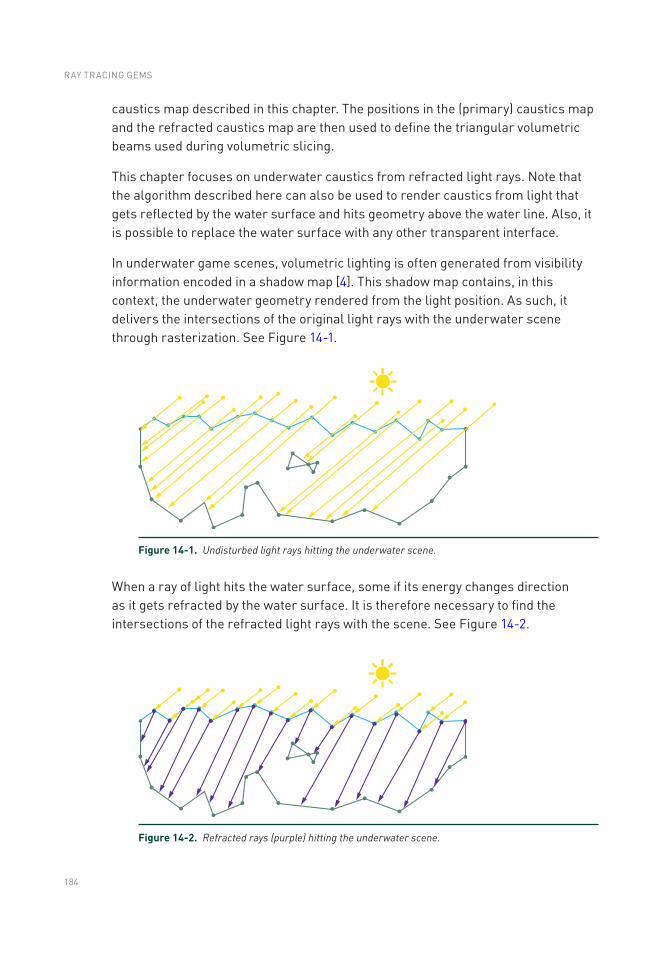
184
caustics map described in this chapter. The positions in the (primary) caustics map and the refracted caustics map are then used to define the triangular volumetric beams used during volumetric slicing.
This chapter focuses on underwater caustics from refracted light rays. Note that the algorithm described here can also be used to render caustics from light that gets reflected by the water surface and hits geometry above the water line. Also, it is possible to replace the water surface with any other transparent interface.
In underwater game scenes, volumetric lighting is often generated from visibility information encoded in a shadow map [4]. This shadow map contains, in this context, the underwater geometry rendered from the light position. As such, it delivers the intersections of the original light rays with the underwater scene through rasterization. See Figure 14-1.
Figure 14-1. Undisturbed light rays hitting the underwater scene.
Figure 14-2. Refracted rays (purple) hitting the underwater scene.
When a ray of light hits the water surface, some if its energy changes direction as it gets refracted by the water surface. It is therefore necessary to find the intersections of the refracted light rays with the scene. See Figure 14-2.
RAY TRACING GEMS
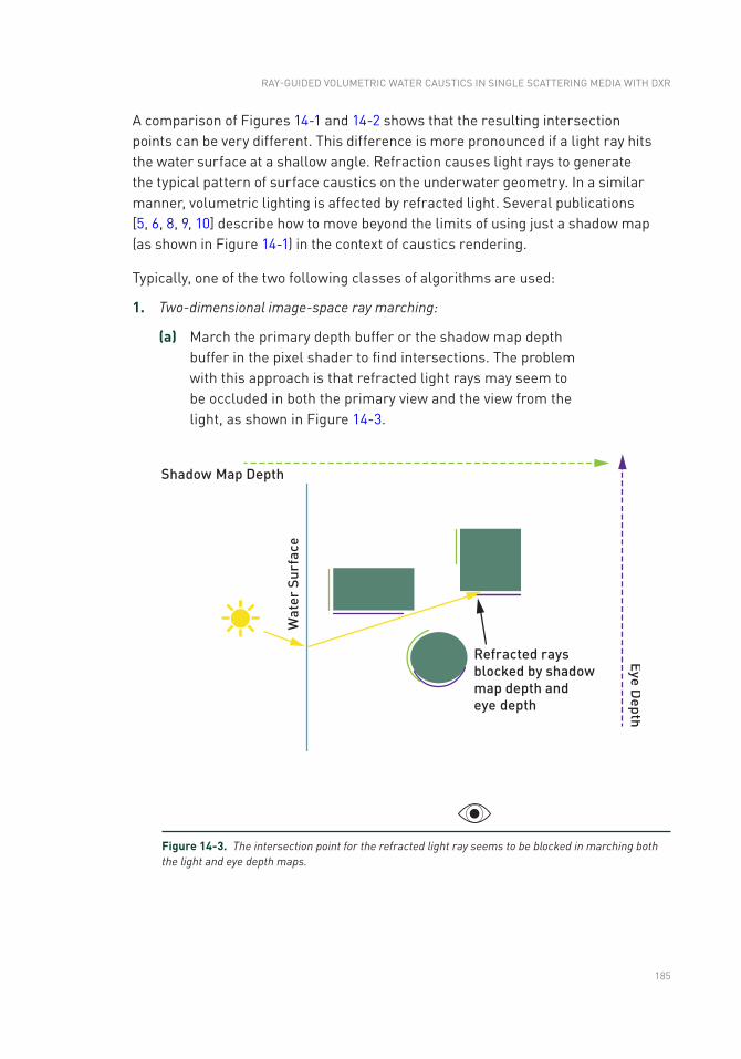
185
A comparison of Figures 14-1 and 14-2 shows that the resulting intersection points can be very different. This difference is more pronounced if a light ray hits the water surface at a shallow angle. Refraction causes light rays to generate the typical pattern of surface caustics on the underwater geometry. In a similar manner, volumetric lighting is affected by refracted light. Several publications [5, 6, 8, 9, 10] describe how to move beyond the limits of using just a shadow map (as shown in Figure 14-1) in the context of caustics rendering.
Typically, one of the two following classes of algorithms are used:
1. Two-dimensional image-space ray marching:
(a) March the primary depth buffer or the shadow map depth buffer in the pixel shader to find intersections. The problem with this approach is that refracted light rays may seem to be occluded in both the primary view and the view from the light, as shown in Figure 14-3.
Figure 14-3. The intersection point for the refracted light ray seems to be blocked in marching both the light and eye depth maps.
RAy-GUIDED VOlUMETRIC WATER CAUSTICS IN SINGlE SCATTERING MEDIA WITH DXR
186
(b) Render and march a set of images using:
i. Multiple depth layers of the primary depth buffer and the shadow map.
ii. Multiple viewpoints of the primary depth buffer and the shadow map.
iii. Distance impostors [8].
Note, however, that these methods increase the runtime cost and the memory consumption. The implementation complexity can be significantly higher than the DXR- based approach described later.
2. Three-dimensional voxel grid marching: This class of algorithms voxelizes the underwater scene and marches the resulting grid. Dependent on grid resolution, these methods can yield impressive results. Voxelization is not a cheap operation and can be interpreted as the rasterization-side equivalent of keeping a bounding volume hierarchy up to date. Memory requirements become prohibitive quickly if high grid resolutions are required. Ray marching a sufficiently detailed 3D grid is not fast and can become prohibitively slow. Overall, the implementation complexity of voxelization methods is higher than the DXR-based approach.
The technique presented in this chapter doesn’t use any of the approximate methods just described to compute the intersections of refracted light rays. Instead, it uses DXR to accurately compute where refracted light rays hit the dynamic underwater scene.
14.2 VOlUMETRIC lIGHTING AND REFRACTED lIGHT
For a general introduction to volumetric lighting computations in participating media, consult the work by Hoobler [4]. Here, we simply present the double integral that describes how much radiance L is scattered toward the eye E from a point S of the underwater scene:
( )( ) ( ) ( ) ( ) ( )E l P E
sS
l e P p E P l P v P d dP| |in, , ,t w s w w w wò ò - + -
W
= - (1)
RAY TRACING GEMS
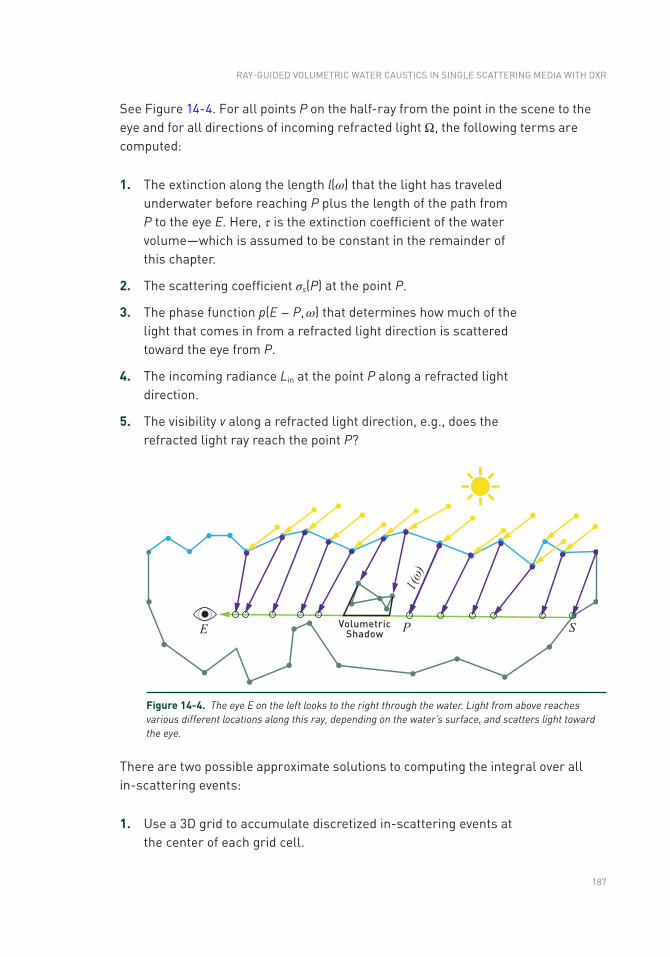
187
See Figure 14-4. For all points P on the half-ray from the point in the scene to the eye and for all directions of incoming refracted light Ω, the following terms are computed:
1. The extinction along the length l(ω) that the light has traveled underwater before reaching P plus the length of the path from P to the eye E. Here, τ is the extinction coefficient of the water volume—which is assumed to be constant in the remainder of this chapter.
2. The scattering coefficient σs(P) at the point P.
3. The phase function p(E − P, ω) that determines how much of the light that comes in from a refracted light direction is scattered toward the eye from P.
4. The incoming radiance Lin at the point P along a refracted light direction.
5. The visibility v along a refracted light direction, e.g., does the refracted light ray reach the point P?
Figure 14-4. The eye E on the left looks to the right through the water. Light from above reaches various different locations along this ray, depending on the water’s surface, and scatters light toward the eye.
There are two possible approximate solutions to computing the integral over all in- scattering events:
1. Use a 3D grid to accumulate discretized in-scattering events at the center of each grid cell.
RAy-GUIDED VOlUMETRIC WATER CAUSTICS IN SINGlE SCATTERING MEDIA WITH DXR
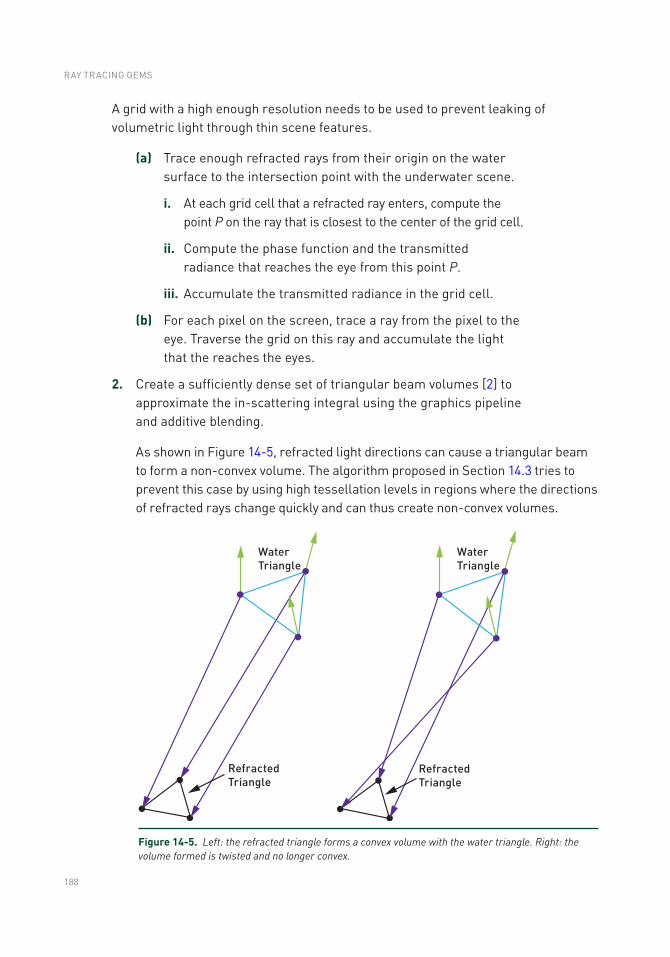
188
Figure 14-5. Left: the refracted triangle forms a convex volume with the water triangle. Right: the volume formed is twisted and no longer convex.
A grid with a high enough resolution needs to be used to prevent leaking of volumetric light through thin scene features.
(a) Trace enough refracted rays from their origin on the water surface to the intersection point with the underwater scene.
i. At each grid cell that a refracted ray enters, compute the point P on the ray that is closest to the center of the grid cell.
ii. Compute the phase function and the transmitted radiance that reaches the eye from this point P.
iii. Accumulate the transmitted radiance in the grid cell.
(b) For each pixel on the screen, trace a ray from the pixel to the eye. Traverse the grid on this ray and accumulate the light that the reaches the eyes.
2. Create a sufficiently dense set of triangular beam volumes [2] to approximate the in- scattering integral using the graphics pipeline and additive blending.
As shown in Figure 14-5, refracted light directions can cause a triangular beam to form a non-convex volume. The algorithm proposed in Section 14.3 tries to prevent this case by using high tessellation levels in regions where the directions of refracted rays change quickly and can thus create non-convex volumes.
RAY TRACING GEMS
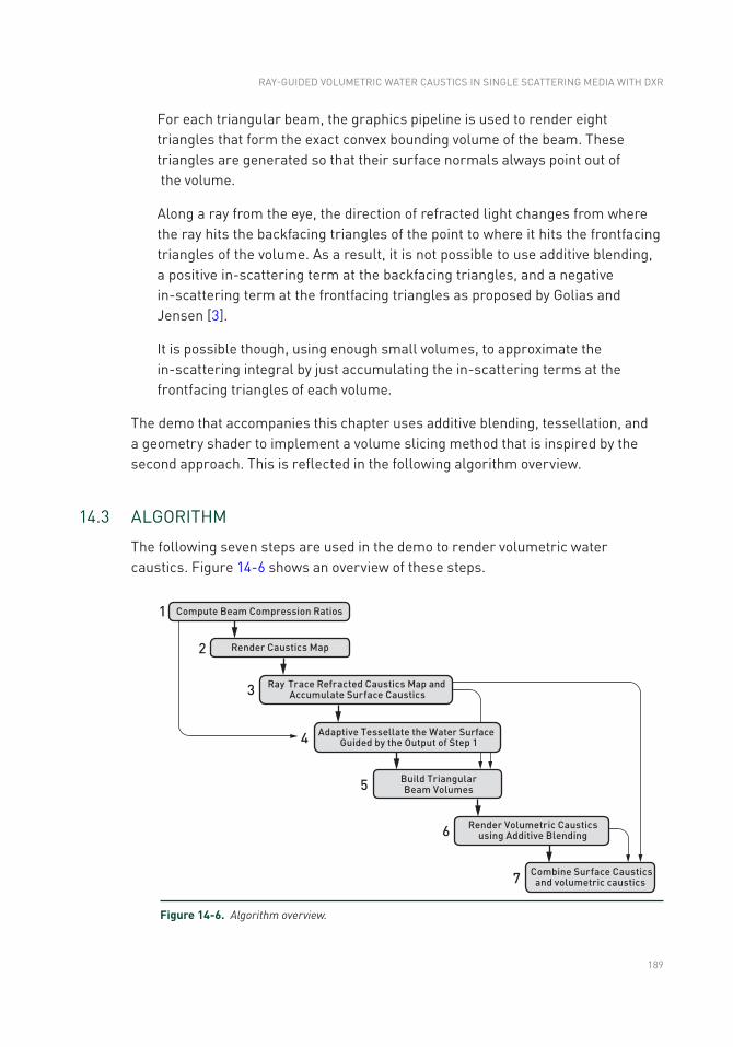
189
For each triangular beam, the graphics pipeline is used to render eight triangles that form the exact convex bounding volume of the beam. These triangles are generated so that their surface normals always point out of the volume.
Along a ray from the eye, the direction of refracted light changes from where the ray hits the backfacing triangles of the point to where it hits the frontfacing triangles of the volume. As a result, it is not possible to use additive blending, a positive in-scattering term at the backfacing triangles, and a negative in-scattering term at the frontfacing triangles as proposed by Golias and Jensen [3].
It is possible though, using enough small volumes, to approximate the in-scattering integral by just accumulating the in-scattering terms at the frontfacing triangles of each volume.
The demo that accompanies this chapter uses additive blending, tessellation, and a geometry shader to implement a volume slicing method that is inspired by the second approach. This is reflected in the following algorithm overview.
14.3 AlGORITHM
The following seven steps are used in the demo to render volumetric water caustics. Figure 14-6 shows an overview of these steps.
Figure 14-6. Algorithm overview.
RAy-GUIDED VOlUMETRIC WATER CAUSTICS IN SINGlE SCATTERING MEDIA WITH DXR
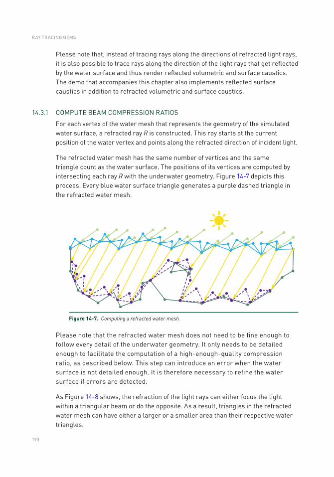
190
Please note that the refracted water mesh does not need to be fine enough to follow every detail of the underwater geometry. It only needs to be detailed enough to facilitate the computation of a high-enough-quality compression ratio, as described below. This step can introduce an error when the water surface is not detailed enough. It is therefore necessary to refine the water surface if errors are detected.
As Figure 14-8 shows, the refraction of the light rays can either focus the light within a triangular beam or do the opposite. As a result, triangles in the refracted water mesh can have either a larger or a smaller area than their respective water triangles.
Please note that, instead of tracing rays along the directions of refracted light rays, it is also possible to trace rays along the direction of the light rays that get reflected by the water surface and thus render reflected volumetric and surface caustics. The demo that accompanies this chapter also implements reflected surface caustics in addition to refracted volumetric and surface caustics.
14.3.1 COMPUTE BEAM COMPRESSION RATIOS
For each vertex of the water mesh that represents the geometry of the simulated water surface, a refracted ray R is constructed. This ray starts at the current position of the water vertex and points along the refracted direction of incident light.
The refracted water mesh has the same number of vertices and the same triangle count as the water surface. The positions of its vertices are computed by intersecting each ray R with the underwater geometry. Figure 14-7 depicts this process. Every blue water surface triangle generates a purple dashed triangle in the refracted water mesh.
Figure 14-7. Computing a refracted water mesh.
RAY TRACING GEMS
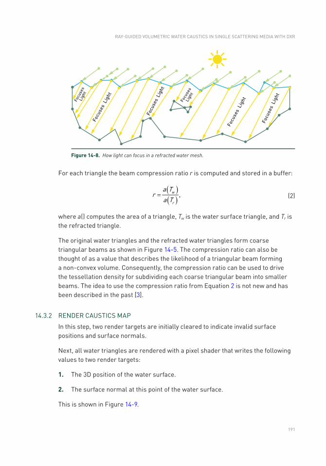
191
For each triangle the beam compression ratio r is computed and stored in a buffer:
( )( )
w
r
a Tr
a T,= (2)
where a() computes the area of a triangle, Tw is the water surface triangle, and Tr is the refracted triangle.
The original water triangles and the refracted water triangles form coarse triangular beams as shown in Figure 14-5. The compression ratio can also be thought of as a value that describes the likelihood of a triangular beam forming a non-convex volume. Consequently, the compression ratio can be used to drive the tessellation density for subdividing each coarse triangular beam into smaller beams. The idea to use the compression ratio from Equation 2 is not new and has been described in the past [3].
14.3.2 RENDER CAUSTICS MAP
In this step, two render targets are initially cleared to indicate invalid surface positions and surface normals.
Next, all water triangles are rendered with a pixel shader that writes the following values to two render targets:
1. The 3D position of the water surface.
2. The surface normal at this point of the water surface.
This is shown in Figure 14-9.
Figure 14-8. How light can focus in a refracted water mesh.
RAy-GUIDED VOlUMETRIC WATER CAUSTICS IN SINGlE SCATTERING MEDIA WITH DXR
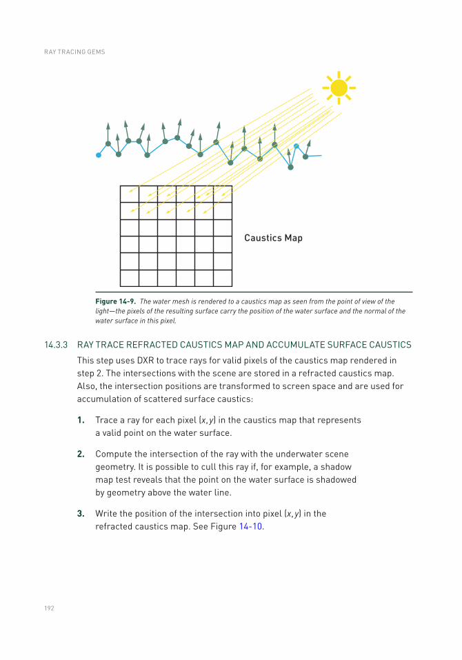
192
14.3.3 RAy TRACE REFRACTED CAUSTICS MAP AND ACCUMUlATE SURFACE CAUSTICS
This step uses DXR to trace rays for valid pixels of the caustics map rendered in step 2. The intersections with the scene are stored in a refracted caustics map. Also, the intersection positions are transformed to screen space and are used for accumulation of scattered surface caustics:
1. Trace a ray for each pixel (x, y) in the caustics map that represents a valid point on the water surface.
2. Compute the intersection of the ray with the underwater scene geometry. It is possible to cull this ray if, for example, a shadow map test reveals that the point on the water surface is shadowed by geometry above the water line.
3. Write the position of the intersection into pixel (x, y) in the refracted caustics map. See Figure 14-10.
Figure 14-9. The water mesh is rendered to a caustics map as seen from the point of view of the light—the pixels of the resulting surface carry the position of the water surface and the normal of the water surface in this pixel.
RAY TRACING GEMS
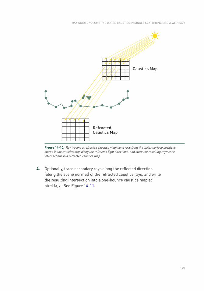
193
Figure 14-10. Ray tracing a refracted caustics map: send rays from the water surface positions stored in the caustics map along the refracted light directions, and store the resulting ray/scene intersections in a refracted caustics map.
4. Optionally, trace secondary rays along the reflected direction (along the scene normal) of the refracted caustics rays, and write the resulting intersection into a one- bounce caustics map at pixel (x, y). See Figure 14-11.
RAy-GUIDED VOlUMETRIC WATER CAUSTICS IN SINGlE SCATTERING MEDIA WITH DXR
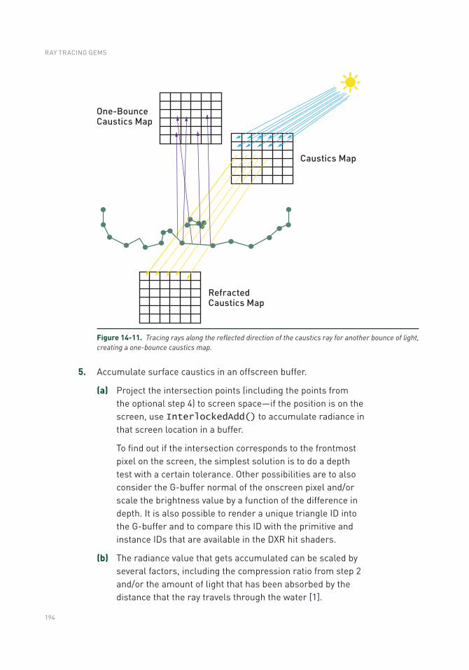
194
5. Accumulate surface caustics in an offscreen buffer.
(a) Project the intersection points (including the points from the optional step 4) to screen space—if the position is on the screen, use InterlockedAdd() to accumulate radiance in that screen location in a buffer.
To find out if the intersection corresponds to the frontmost pixel on the screen, the simplest solution is to do a depth test with a certain tolerance. Other possibilities are to also consider the G-buffer normal of the onscreen pixel and/or scale the brightness value by a function of the difference in depth. It is also possible to render a unique triangle ID into the G-buffer and to compare this ID with the primitive and instance IDs that are available in the DXR hit shaders.
(b) The radiance value that gets accumulated can be scaled by several factors, including the compression ratio from step 2 and/or the amount of light that has been absorbed by the distance that the ray travels through the water [1].
Figure 14-11. Tracing rays along the reflected direction of the caustics ray for another bounce of light, creating a one-bounce caustics map.
RAY TRACING GEMS
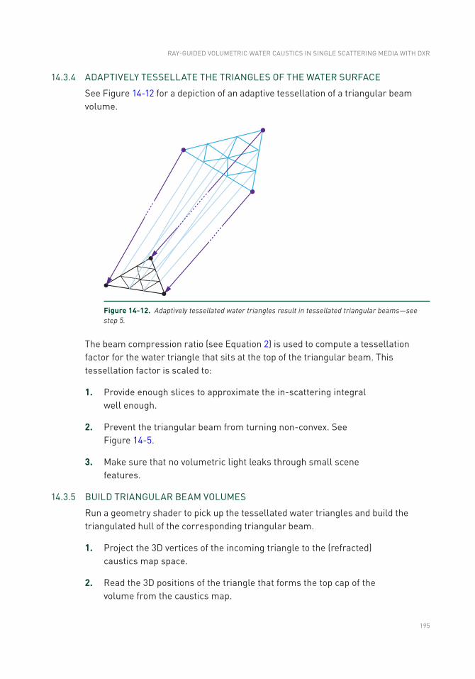
195
14.3.4 ADAPTIVEly TESSEllATE THE TRIANGlES OF THE WATER SURFACE
See Figure 14-12 for a depiction of an adaptive tessellation of a triangular beam volume.
Figure 14-12. Adaptively tessellated water triangles result in tessellated triangular beams—see step 5.
The beam compression ratio (see Equation 2) is used to compute a tessellation factor for the water triangle that sits at the top of the triangular beam. This tessellation factor is scaled to:
1. Provide enough slices to approximate the in-scattering integral well enough.
2. Prevent the triangular beam from turning non-convex. See Figure 14-5.
3. Make sure that no volumetric light leaks through small scene features.
14.3.5 BUIlD TRIANGUlAR BEAM VOlUMES
Run a geometry shader to pick up the tessellated water triangles and build the triangulated hull of the corresponding triangular beam.
1. Project the 3D vertices of the incoming triangle to the (refracted) caustics map space.
2. Read the 3D positions of the triangle that forms the top cap of the volume from the caustics map.
RAy-GUIDED VOlUMETRIC WATER CAUSTICS IN SINGlE SCATTERING MEDIA WITH DXR
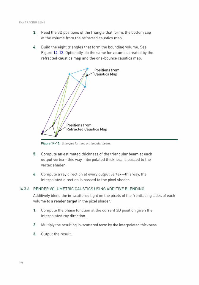
196
3. Read the 3D positions of the triangle that forms the bottom cap of the volume from the refracted caustics map.
4. Build the eight triangles that form the bounding volume. See Figure 14-13. Optionally, do the same for volumes created by the refracted caustics map and the one-bounce caustics map.
5. Compute an estimated thickness of the triangular beam at each output vertex—this way, interpolated thickness is passed to the vertex shader.
6. Compute a ray direction at every output vertex—this way, the interpolated direction is passed to the pixel shader.
14.3.6 RENDER VOlUMETRIC CAUSTICS USING ADDITIVE BlENDING
Additively blend the in-scattered light on the pixels of the frontfacing sides of each volume to a render target in the pixel shader.
1. Compute the phase function at the current 3D position given the interpolated ray direction.
2. Multiply the resulting in-scattered term by the interpolated thickness.
3. Output the result.
Figure 14-13. Triangles forming a triangular beam.
RAY TRACING GEMS
197
14.3.7 COMBINE SURFACE CAUSTICS AND VOlUMETRIC CAUSTICS
This step combines the image of the scene that has been lit by the surface caustics and a blurred version of the volumetric caustics that has been rendered using additive blending.
1. Blur/denoise the surface caustics from step 3.
2. Use the denoised surface caustics buffer to shed light on the scene, e.g., multiply it by the albedo texture of the G-buffer pixel and add it to the unlit result to produce a lit G-buffer.
3. Blur the result from step 6 slightly and add it to the lit G-buffer.
14.4 IMPlEMENTATION DETAIlS
As described in Section 14.1, the DirectX 12 DXR API is used to implement all ray tracing workloads. For step 1, DispatchRays() is called so that each thread traces exactly one refracted ray into the scene. The resulting refracted water mesh is written to a buffer that is read by later steps and uses the same index buffer as the original water mesh.
Step 2 is implemented as a normal rasterization pass. For step 3, DispatchRays() is called to cast a ray for every valid pixel of the caustics map from step 2. Optionally, the shader casts additional rays along the reflected direction for surface caustics that are generated by light rays that get reflected by the water surface or the one-bounce caustics map. Accumulation of refracted/reflected light happens in a half-resolution buffer to facilitate fast denoising.
If an additional bounce of caustics is selected, yet another ray is cast in step 2 to simulate the reflection of caustics rays by the scene. The resulting intersections of these reflected rays are used to simulate indirect lighting through surface caustics and are written to another caustics map, the reflected caustics map—the buffer is sized to facilitate drawing volumetric beams for this additional bounce.
Volumetric caustics are accumulated in step 6 in a half-resolution buffer to speed up the drawing of the triangular beams. The geometry shader in step 5 creates triangular beams for the primary refracted caustics as well as for the optional additional bounce recorded in the one-bounce caustics map.
Denoising of the surface caustics buffer in step 7 is done through a set of iterated cross-bilateral blurring steps that account for differences in view-space depth, normals, and positions. Finally, surface caustics and volumetric caustics are upsampled bilaterally and get combined with the rendered scene.
RAy-GUIDED VOlUMETRIC WATER CAUSTICS IN SINGlE SCATTERING MEDIA WITH DXR
198
14.5 RESUlTS
Table 14-1 shows caustics workload timings taken in a scene for four different camera positions and light setups on an NVIDIA RTX 2080 Ti board running caustics workloads at a resolution of 1920 × 1080 using the official DXR API that is part of DirectX 12.
Screenshots from these four scenes are shown in Figure 14-14. All scenes run at interactive frame rates in excess of 60 FPS while casting rays from the pixels of a 2048 × 2048 caustics map. The timings from Table 14-1 indicate that volumetric caustics operate, in most cases, within a time span that is acceptable for integration in a modern computer game. In comparison, the work from liktor and Dachsbacher [6] was not able to reach a performance level that made integration into games feasible.
> The top left screenshot in Figure 14-14 shows a view from above the water line. In this screenshot refracted volumetric underwater caustics and reflected caustics that are visible above the water line are generated by the algorithm described in this chapter. The caustics workloads for this image amount to a total time of 2.9 ms.
> The top right screenshot in Figure 14-14 shows a view from below the water line. For this scene refracted volumetric underwater caustics and a secondary volumetric bounce of light are rendered. For this scenario the volumetric bounce and high maximum tessellation factor preset cause the timing for the volumetric part of the caustics rendering to climb to 4.6 ms. These settings are currently too expensive to be used inside a game.
> The bottom left screenshot in Figure 14-14 shows again a view from below the water line. For this scene again refracted volumetric underwater caustics and a secondary volumetric bounce of light are rendered. For this scenario, the second volumetric bounce along with a moderately high maximum tessellation factor preset cause the timing for the volumetric part of the caustics rendering to climb to a more moderate 2.1 ms. These settings are probably acceptable within a game that focuses on high-quality volumetric caustics.
> The bottom right screenshot in Figure 14-14 shows another view from below the water line. For this scenario the second volumetric bounce along with a moderately high maximum tessellation factor preset cause the timing for the volumetric part of the caustics rendering to take only 1.4 ms. Please note how the second bounce of light casts light onto the downward-facing part of the character.
RAY TRACING GEMS
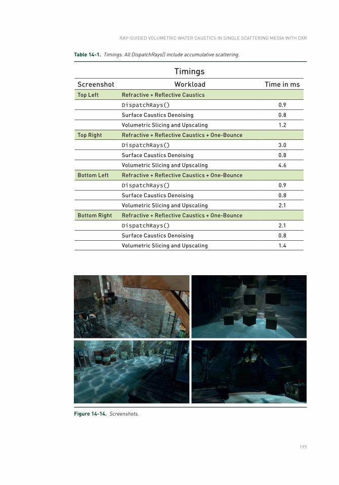
199
Figure 14-14. Screenshots.
Table 14-1. Timings. All DispatchRays() include accumulative scattering.
RAy-GUIDED VOlUMETRIC WATER CAUSTICS IN SINGlE SCATTERING MEDIA WITH DXR
200
14.6 FUTURE WORK
In the current demo implementation, the caustics map and the refracted caustics map need to have a resolution that is high enough to capture the underwater geometry in enough detail. It would be interesting to investigate how ideas from Wyman and Nichols [10] or liktor and Dachsbacher [6] could be used to adaptively cast rays.
Further on, instead of using the rasterization pipeline to slice the parts of the water volume that concentrate light, it could be faster to accumulate in-scattered light in a volumetric texture. For a position on a ray to the eye, the information stored in the caustics map and the refracted caustics map could be used to prevent volumetric light leaking through thin features of a scene.
14.7 DEMO
A demo that can be run on NVIDIA GPUs showcasing the proposed technique is provided in the code repository.
REFERENCES
[1] Baboud, l., and Décoret, X. Realistic Water Volumes in Real-Time. In Eurographics Conference on Natural Phenomena (2006), pp. 25–32.
[2] Ernst, M., Akenine-Möller, T., and Jensen, H. W. Interactive Rendering of Caustics Using Interpolated Warped Volumes. In Graphics Interface (2005), pp. 87–96.
[3] Golias, R., and Jensen, l. S. Deep Water Animation and Rendering. https://www.gamasutra.com/view/feature/131445/deep_water_animation_and_rendering.
php, 2001.
[4] Hoobler, N. Fast, Flexible, Physically-Based Volumetric light Scattering. https://developer.nvidia.com/sites/default/files/akamai/gameworks/downloads/
papers/NVVL/Fast_Flexible_Physically-Based_Volumetric_Light_Scattering.
pdf, 2016.
[5] Hu, W., Dong, Z., Ihrke, I., Grosch, T., yuan, G., and Seidel, H.-P. Interactive Volume Caustics in Single-Scattering Media. In Symposium on Interactive 3D Graphics and Games (2010), pp. 109–117.
[6] liktor, G., and Dachsbacher, C. Real-Time Volume Caustics with Adaptive Beam Tracing. In Symposium on Interactive 3D Graphics and Games (2011), pp. 47–54.
RAY TRACING GEMS

201
[7] Shah, M. A., Konttinen, J., and Pattanaik, S. Caustics Mapping: An Image-Space Technique for Real-Time Caustics. IEEE Transactions on Visualization and Computer Graphics 13, 2 (March 2007), 272–280.
[8] Szirmay-Kalos, l., Aszódi, B., lazányi, I., and Premecz, M. Approximate Ray-Tracing on the GPU with Distance Impostors. Computer Graphics Forum 24, 3 (2005), 695–704.
[9] Wang, R., Wang, R., Zhou, K., Pan, M., and Bao, H. An Efficient GPU-based Approach for Interactive Global Illumination. ACM Transactions on Graphics 28, 3 (July 2009), 91:1–91:8.
[10] Wyman, C., and Nichols, G. Adaptive Caustic Maps Using Deferred Shading. Computer Graphics Forum 28, 2 (Apr. 2009), 309–318.
Open Access This chapter is licensed under the terms of the Creative Commons Attribution-NonCommercial-NoDerivatives 4.0 International license (http://creativecommons.org/licenses/by-nc-nd/4.0/), which permits any noncommercial use, sharing, distribution and
reproduction in any medium or format, as long as you give appropriate credit to the original author(s) and the source, provide a link to the Creative Commons license and indicate if you modified the licensed material. you do not have permission under this license to share adapted material derived from this chapter or parts of it.
The images or other third party material in this chapter are included in the chapter's Creative Commons license, unless indicated otherwise in a credit line to the material. If material is not included in the chapter's Creative Commons license and your intended use is not permitted by statutory regulation or exceeds the permitted use, you will need to obtain permission directly from the copyright holder.
RAy-GUIDED VOlUMETRIC WATER CAUSTICS IN SINGlE SCATTERING MEDIA WITH DXR
PART IV
SAMPLING
205
PART IV
Sampling
Ray tracing is all about sampling, and sampling is the basic operation of computing averages. Similarly to conducting a survey, it is important whom you ask, as this determines how reliable your statistics will be.
Chapter 15, “On the Importance of Sampling,” takes you on a tour through some useful integrals in graphics that are computed by averaging. You will learn why sampling matters, how variance decreases and may be decreased, and why a denoiser is becoming inevitable.
The journey then takes you to Chapter 16, the “Sampling Transformations Zoo.” We will walk you through a collection of useful code snippets that let you transform uniformly distributed samples according to a desired density or onto a piece of geometry. It is the perfect complement for all the sampling tasks that you need to complete when crafting your own rendering algorithm based on ray tracing.
Not everything turns out nice with sampling. And in fact, Chapter 17, “Ignoring the Inconvenient When Tracing Rays,” will help you very much understand what can go wrong with sampling. There is a simple way for you to fix things, and a second alternative that at least does not destroy all rendering mathematics. All in all, this chapter provides crucial and battle-proven insight.
As an example of how to put things together, Chapter 18, “Importance Sampling of Many Lights on the GPU,”, provides a fast implementation of a modern algorithm to deal with illumination by many lights. This has been a classic challenge in rendering movies that now enters the domain of real-time image synthesis. This chapter is an excellent starting point for your own development.
There is so much more to learn about sampling. Do not forget to check out the references to Monte Carlo and quasi-Monte Carlo integration in these sampling chapters!
Alexander Keller
207© NVIDIA 2019 E. Haines, T. Akenine-Möller (eds.), Ray Tracing Gems, https://doi.org/10.1007/978-1-4842-4427-2_15
CHAPTER 15
On the Importance of SamplingMatt Pharr NVIDIA
ABSTRACT
With the recent arrival of ray tracing to the real-time graphics pipeline, developers are faced with a new challenge: figuring out how to make the most of the rays that they’re able to trace. One important question to decide is for which lighting effects to trace rays—choices include shadows, reflections, ambient occlusion, and full global illumination.
Another important question is how to choose which rays to trace for the chosen effect; an introduction to that question is the topic of this chapter. In the following, we will see how most lighting calculations in rendering can be interpreted as estimating the values of integrals and how tracing rays is a natural fit to an effective numerical integration technique: Monte Carlo. Given some background in Monte Carlo integration, we then see how well-chosen rays can dramatically improve the speed of convergence, which in turn can either improve overall system performance—by getting the same quality result for fewer rays—or improve image quality—by getting lower error from the same number of rays.
15.1 INTRODUCTION
With the introduction of DirectX Raytracing (DXR) at the 2018 Game Developers Conference and then the launch of NVIDIA’s RTX GPUs in the summer of 2018, ray tracing has unequivocally arrived for real-time rendering. This is one of the greatest changes the real-time graphics pipeline has seen: after always offering rasterization as the only visibility algorithm, now a second visibility algorithm has been added—ray tracing.
Ray tracing and rasterization complement each other well. Rasterization remains a high-performance way to perform coherent visibility computations: it assumes a single viewpoint (possibly a single homogeneous viewpoint, for an orthographic view), and it regularly samples visibility over a pixel grid. Together, these properties allow high- performance hardware implementations that amortize per-triangle work over multiple pixels and incrementally compute depth and coverage from pixel to pixel.
208
In contrast, ray tracing allows fully incoherent visibility computations. Each ray traced can have an arbitrary origin and direction; the hardware places no restrictions on them.
With ray tracing in hand, the task for developers is to figure out how best to use it. GPU ray tracing hardware provides a few visibility primitives: “What is the first thing visible from this point in this direction?” “Is there anything blocking the straight line segment between these two points?” However, it does not dictate how it should be used for image synthesis—it is up to developers to decide how to do that. In a sense, the situation is similar to programmable shading on GPUs: the hardware provides the basic computational capabilities, and it is up to developers to decide the best way to use those for their applications.
To help motivate some of the trade-offs involved in choosing which rays to trace, we start by looking at a basic ambient occlusion computation through the lens of Monte Carlo integration. We will see how different sampling techniques (and thus different rays traced) lead to different amounts of error in the results before moving on to see the application of some of these ideas to direct illumination from area light sources.
Sampling well for rendering is a complex topic—whole books have been written on the topic and it remains an active area of research. Thus, this chapter can only scratch the surface of the topic, but it includes pointers to resources that provide more information along the way.
15.2 EXAMPLE: AMBIENT OCCLUSION
Most computations related to light and reflection and graphics can be understood as integration problems: for example, we integrate the product of incident light arriving at all directions over the hemisphere at a point with the bidirectional scattering distribution function (BSDF) that describes reflection at the point in order to compute reflected light from a surface.
Monte Carlo integration has been shown to be an effective method for these integration tasks in rendering. It is a statistical technique based on taking a weighted average of random samples of the integrand. Monte Carlo is a good choice for rendering because it works well with high-dimensional integrals (as we end up encountering with global illumination), places few restrictions on the functions to which it can be applied, and only requires point-wise evaluation of them. See the book by Sobol [5] for an approachable introduction to the topic.
Sampling is a perfect fit for ray tracing—it corresponds directly to queries like “is the light source visible in this direction?”or “what is the first visible surface in this direction?”
RAY TRACING GEMS
209
Here is the definition of the basic Monte Carlo estimator with k samples, which gives a method for computing an approximation to an n-dimensional integral of some function f:
( ) ( )n
k
i ,i
E f X f x xk [0 1]
1
1 d .ò=
é ù=ê ú
ë ûå (1)
On the left-hand side of the equality, we have E, which denotes the expected value; the idea is that it indicates that, statistically, the quantity in square brackets is expected to take on the value of the expression on the right-hand side. Sometimes it may be larger and sometimes it may be smaller, but we can imagine that in the limit of more and more values, we expect its average to converge.
The expression inside the square brackets is an average of values of f using a set of independent random variables Xi that take on all values in [0, 1]n with uniform probability. In an implementation, each Xi might just be an n-dimensional random number, but here, writing the Monte Carlo estimator in terms of random variables is what allows rigorous discussion of the expected value.
We have now an easy-to-implement way to estimate the value of any integral. Let us apply it to ambient occlusion, a useful shading technique that gives a reasonable approximation to some global lighting effects. We define the ambient occlusion function a at a point P as
( ) ( )da P v1 cos d ,w q wpòW
= (2)
where vd is a visibility function that is zero if a ray from P in the direction ω is occluded at a distance less than d and one otherwise, where Ω denotes the hemisphere of directions around the surface normal at P, and where the angle θ is measured with respect to the surface normal. The 1
p term ensures that the value
of a(P) is between zero and one.
Consider now the application of the basic Monte Carlo estimator to ambient occlusion. Here, we integrate over the hemisphere rather than a [0, 1)n domain, but it is not too hard to use a few changes of variables to show that the estimator applies to other integration domains as well. Our estimator is
( ) ( )k
d i ii
a P E vk 1
1 1 cos ,w q=
é ù= ê úpë û
å (3)
where ωi are random directions over the hemisphere, each one chosen with uniform probability.
ON THE IMPORTANCE OF SAMPLING
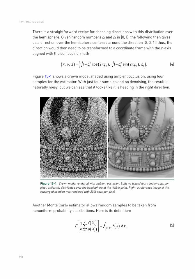
210
There is a straightforward recipe for choosing directions with this distribution over the hemisphere. Given random numbers ξ1 and ξ2 in [0, 1), the following then gives us a direction over the hemisphere centered around the direction (0, 0, 1) (thus, the direction would then need to be transformed to a coordinate frame with the z-axis aligned with the surface normal):
( ) ( ) ( )( )x, y , z , ,2 21 2 1 2 11 cos 2 1 sin 2 .x x x x x= - p - p (4)
Figure 15-1 shows a crown model shaded using ambient occlusion, using four samples for the estimator. With just four samples and no denoising, the result is naturally noisy, but we can see that it looks like it is heading in the right direction.
Figure 15-1. Crown model rendered with ambient occlusion. Left: we traced four random rays per pixel, uniformly distributed over the hemisphere at the visible point. Right: a reference image of the converged solution was rendered with 2048 rays per pixel.
Another Monte Carlo estimator allows random samples to be taken from nonuniform probability distributions. Here is its definition:
( )( ) ( )n
ki
,i i
f XE f x x
k p X [0 1]1
1 d .ò=
é ù=ê ú
ê úë ûå (5)
RAY TRACING GEMS
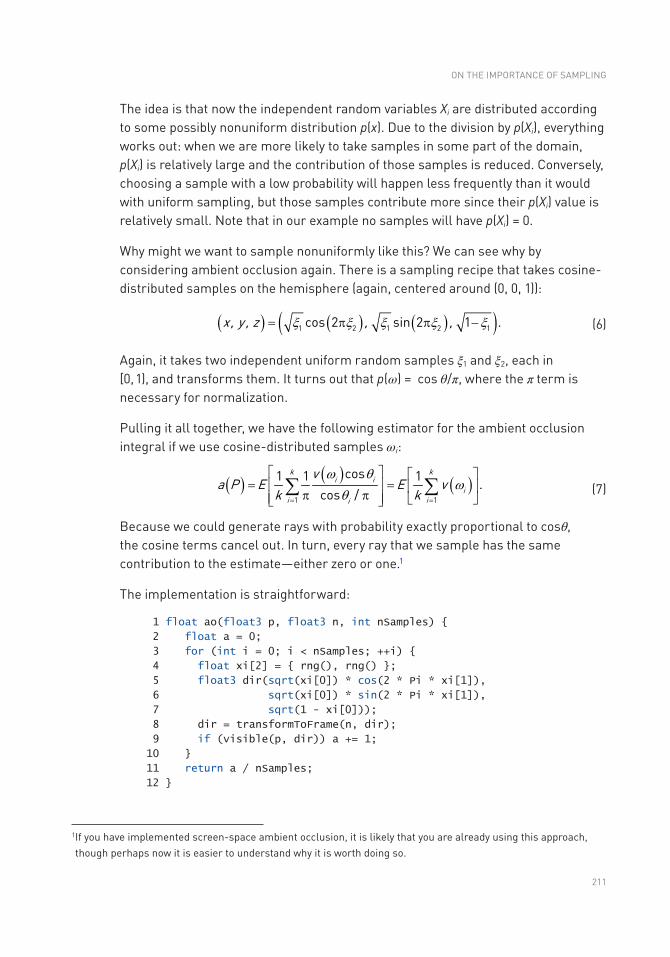
211
The idea is that now the independent random variables Xi are distributed according to some possibly nonuniform distribution p(x). Due to the division by p(Xi), everything works out: when we are more likely to take samples in some part of the domain, p(Xi) is relatively large and the contribution of those samples is reduced. Conversely, choosing a sample with a low probability will happen less frequently than it would with uniform sampling, but those samples contribute more since their p(Xi) value is relatively small. Note that in our example no samples will have p(Xi) = 0.
Why might we want to sample nonuniformly like this? We can see why by considering ambient occlusion again. There is a sampling recipe that takes cosine- distributed samples on the hemisphere (again, centered around (0, 0, 1)):
( ) ( ) ( )( )x, y , z , ,1 2 1 2 1cos 2 sin 2 1 .x x x x x= p p - (6)
Again, it takes two independent uniform random samples ξ1 and ξ2, each in [0, 1), and transforms them. It turns out that p(ω) = cos θ/π, where the π term is necessary for normalization.
Pulling it all together, we have the following estimator for the ambient occlusion integral if we use cosine-distributed samples ωi:
( ) ( ) ( )k k
i ii
i ii
va P E E v
k k1 1
cos1 1 1 .cos /
w qw
q= =
é ù é ù= =ê ú ê úp pê ú ë ûë û
å å (7)
Because we could generate rays with probability exactly proportional to cosθ, the cosine terms cancel out. In turn, every ray that we sample has the same contribution to the estimate—either zero or one.1
The implementation is straightforward:
1 float ao(float3 p, float3 n, int nSamples)
2 float a = 0;
3 for (int i = 0; i < nSamples; ++i)
4 float xi[2] = rng(), rng() ;
5 float3 dir(sqrt(xi[0]) * cos(2 * Pi * xi[1]),
6 sqrt(xi[0]) * sin(2 * Pi * xi[1]),
7 sqrt(1 - xi[0]));
8 dir = transformToFrame(n, dir);
9 if (visible(p, dir)) a += 1;
10
11 return a / nSamples;
12
1 If you have implemented screen-space ambient occlusion, it is likely that you are already using this approach, though perhaps now it is easier to understand why it is worth doing so.
ON THE IMPORTANCE OF SAMPLING
212
Figure 15-2 shows the crown model again, now comparing uniform sampling to cosine-distributed sampling. Cosine-distributed sampling has visibly lower error. Why might this be?
With uniformly distributed sampling, some of the rays turn out to have an insignificant contribution. Consider a ray close to the horizon: its value of cosθ will be close to zero, and effectively, we learn little by tracing the ray. Its contribution to the sum in the estimator will either be zero or minimal. Put another way, we do just as much work to trace those rays as all the other rays, but we do not get much out of them. The difference in the amount of computation required to sample rays between the two techniques is negligible, so there is no reason not to use the more effective sampling technique.
This general technique, sampling from a distribution that is similar to the integrand, is called importance sampling and is an important technique for efficient Monte Carlo integration in rendering. The closer a match p(x) is to f(x), the better the results. However, if p(x) does not match f(x) well, error will increase as the encountered ratios f(x)/p(x) oscillate between minuscule and huge values. As long as p(x) > 0 whenever f(x) ≠ 0, the result will still be correct in the limit, though the error may be high enough for that to be a small consolation.
Figure 15-2. Crown model rendered with ambient occlusion: uniform sampling (left) and cosine-weighted sampling (right). Both used four rays per pixel. Cosine- weighted sampling has nearly 30% lower average pixel error than uniform sampling, which is reflected in its image having noticeably less noise.
RAY TRACING GEMS
213
15.3 UNDERSTANDING VARIANCE
A concept called variance is useful for characterizing the expected error in Monte Carlo integration. The variance of a random variable X is defined in terms of another expectation:
( )é ù é ùé ù º - é ù = - é ùë û ë û ë ûë ûê úë ûV X E X E X E X E X
2 22 . (8)
Variance is thus a measure of the squared difference between a random variable and its expected value (i.e., its average). In other words, if a random variable has low variance, then most of the time its value is close to its average (and the converse if variance is high).
If we can accurately compute the expectation of a random variable (e.g., using Monte Carlo integration with a large number of samples), we can compute an estimate of the variance directly using Equation 8.
We can also estimate the variance: given a number of independent values of a random variable, we can compute the sample variance from them using Equation 8 with a small adjustment. The following code illustrates the computation:
1 float estimate_sample_variance(float samples[], int n)
2 float sum = 0, sum_sq = 0;
3 for (int i = 0; i < n; ++i)
4 sum += samples[i];
5 sum_sq += samples[i] * samples[i];
6
7 return sum_sq / (n * (n - 1))) -
8 sum * sum / ((n - 1) * n * n);
9
Note that it is not necessary to store all the samples: sample variance can also be computed incrementally by keeping track of the sum and squared sum of the values of the random variable and the total number of samples.
One challenge with the sample variance is that it has variance itself: if we happened to have a number of similar sample values even though the underlying estimator had high variance, we would compute a much-too-low estimate of the sample variance.
Variance is a particularly useful concept in Monte Carlo integration, as there is a fundamental relationship between variance and the number of samples taken: for random samples, variance decreases linearly with the number of samples taken.2
2 Variance can decrease even faster with certain carefully constructed sampling patterns, especially if the integrand is smooth, though we ignore that for the discussion here.
ON THE IMPORTANCE OF SAMPLING
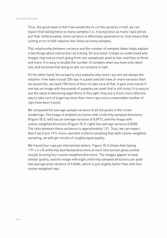
214
Thus, the good news is that if we would like to cut the variance in half, we can expect that taking twice as many samples (i.e., tracing twice as many rays) will do just that. Unfortunately, since variance is effectively squared error, that means that cutting error in half requires four times as many samples.
This relationship between variance and the number of samples taken helps explain a few things about interactive ray tracing. On one hand, it helps us understand why images improve so much going from one sample per pixel to two, and then to three and more. It is easy to double the number of samples when you have only taken one, and we know that doing so will cut variance in half.
On the other hand, this property also explains why more rays are not always the solution: if we have traced 128 rays in a pixel and still have 2× more variance than we would like, we need 128 more of them to take care of that. It gets even worse if one has an image with thousands of samples per pixel that is still noisy! It is easy to see the value of denoising algorithms in this light; they are a much more effective way to take care of lingering noise than more rays once a reasonable number of rays have been traced.
We computed the average sample variance of all the pixels in the crown renderings. The image of ambient occlusion with uniformly sampled directions (Figure 15-2, left) has an average variance of 0.0972, and the image with cosine-weighted directions (Figure 15-2, right) has average variance 0.0508. The ratio between these variances is approximately 1.91. Thus, we can expect that if we trace 1.91× more rays with uniform sampling than with cosine-weighted sampling, we will get results of roughly equal quality.
We traced four rays per intersection before. Figure 15-3 shows that having 1.91 × 4 ≈ 8 uniformly distributed directions at each intersection gives similar results to using four cosine-weighted directions. The images appear to have similar quality, and the image with eight uniformly sampled directions per pixel has average pixel variance of 0.0484, which is just slightly better than with four cosine-weighted rays.
RAY TRACING GEMS
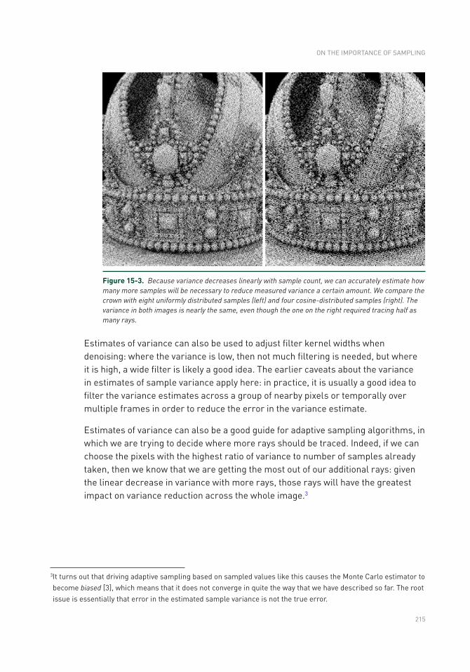
215
Estimates of variance can also be used to adjust filter kernel widths when denoising: where the variance is low, then not much filtering is needed, but where it is high, a wide filter is likely a good idea. The earlier caveats about the variance in estimates of sample variance apply here: in practice, it is usually a good idea to filter the variance estimates across a group of nearby pixels or temporally over multiple frames in order to reduce the error in the variance estimate.
Estimates of variance can also be a good guide for adaptive sampling algorithms, in which we are trying to decide where more rays should be traced. Indeed, if we can choose the pixels with the highest ratio of variance to number of samples already taken, then we know that we are getting the most out of our additional rays: given the linear decrease in variance with more rays, those rays will have the greatest impact on variance reduction across the whole image.3
3 It turns out that driving adaptive sampling based on sampled values like this causes the Monte Carlo estimator to become biased [3], which means that it does not converge in quite the way that we have described so far. The root issue is essentially that error in the estimated sample variance is not the true error.
Figure 15-3. Because variance decreases linearly with sample count, we can accurately estimate how many more samples will be necessary to reduce measured variance a certain amount. We compare the crown with eight uniformly distributed samples (left) and four cosine-distributed samples (right). The variance in both images is nearly the same, even though the one on the right required tracing half as many rays.
ON THE IMPORTANCE OF SAMPLING
216
15.4 DIRECT ILLUMINATION
Another important integral in rendering comes from the surface scattering equation, which gives the scattered radiance at a point P in a direction ωo due to the incident radiance function Li(P, ω) and the BSDF f(ω → ωo):
( ) ( ) ( )o o i oL P, L P, f cos d .w w w w q wòW
= ® (9)
In this section, we consider the effect of a few different sampling choices when estimating the value of this integral and measure their effect on variance.
Ideally, we would like to be able to sample directions ω proportionally to the value of the product of Li, f, and cosθ. In general, this is difficult to do, especially because the incident radiance function generally is not available in closed form—we need to trace rays to evaluate it.
Here, we make a few simplifications. First, we only consider the incident light from emitters in the scene and ignore indirect illumination. Second, we only look at the effect of various choices in sampling proportional to Li. Note that the second simplification absolutely should not be used in practice: it is imperative to also sample from the BSDF and to use a powerful variance reduction technique called multiple importance sampling to weight the samples [6].
With those simplifications, we are left with the task of computing the value of the following Monte Carlo estimator:
( ) ( ) ( )( )
ki i i o i
o oi i
L P, fL P, E
k p1
cos1 ,w w w q
ww=
é ù®= ê ú
ê úë ûå (10)
where the ωi have been sampled from some distribution p(ω). Note that if we only consider direct illumination, there is no reason to sample a direction that definitely does not intersect a light source. Thus, a reasonable strategy is to sample according to a distribution over the surface of the light, to choose a point on the light source, and then to set the direction ωi as the direction from P to the sampled point.
RAY TRACING GEMS
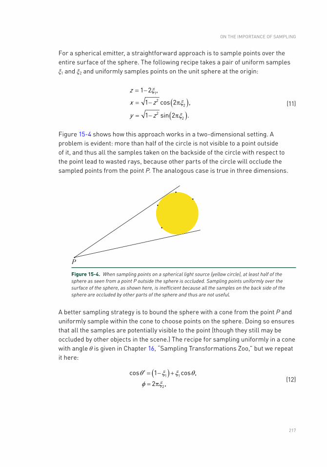
217
For a spherical emitter, a straightforward approach is to sample points over the entire surface of the sphere. The following recipe takes a pair of uniform samples ξ1 and ξ2 and uniformly samples points on the unit sphere at the origin:
( )( )
x z
y z
z 1
22
22
1 2
1 co
,
s 2 ,
1 sin 2 .
x
x
x
-
- p
= - p
=
= (11)
Figure 15-4 shows how this approach works in a two-dimensional setting. A problem is evident: more than half of the circle is not visible to a point outside of it, and thus all the samples taken on the backside of the circle with respect to the point lead to wasted rays, because other parts of the circle will occlude the sampled points from the point P. The analogous case is true in three dimensions.
A better sampling strategy is to bound the sphere with a cone from the point P and uniformly sample within the cone to choose points on the sphere. Doing so ensures that all the samples are potentially visible to the point (though they still may be occluded by other objects in the scene.) The recipe for sampling uniformly in a cone with angle θ is given in Chapter 16, “Sampling Transformations Zoo,” but we repeat it here:
( )1 1
2
cos 1 cos ,
2 ,
q x x q
f x
= +
= p
¢ - (12)
Figure 15-4. When sampling points on a spherical light source (yellow circle), at least half of the sphere as seen from a point P outside the sphere is occluded. Sampling points uniformly over the surface of the sphere, as shown here, is inefficient because all the samples on the back side of the sphere are occluded by other parts of the sphere and thus are not useful.
ON THE IMPORTANCE OF SAMPLING
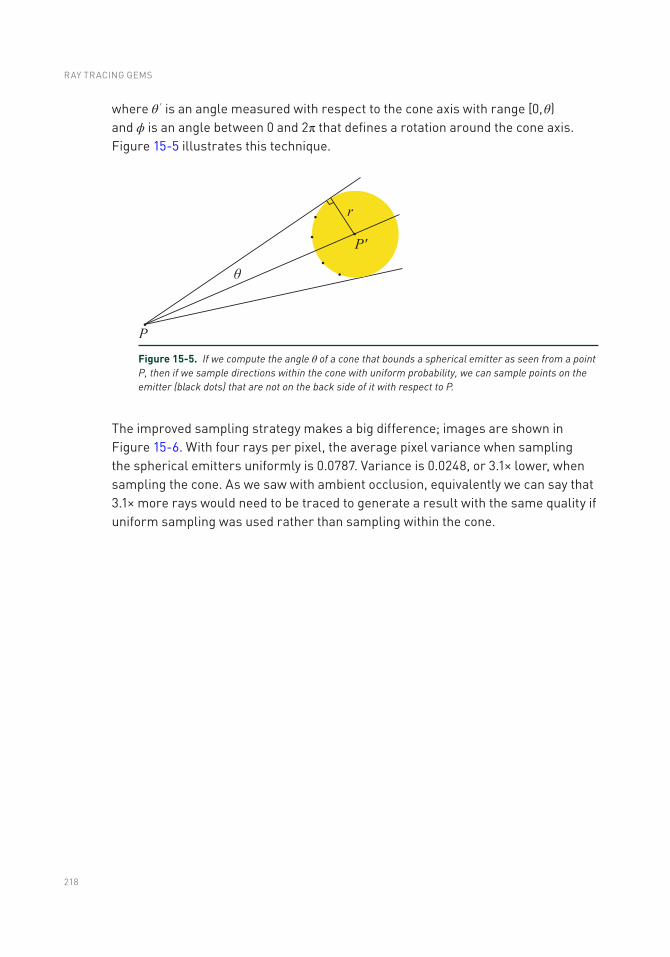
218
where θ ′ is an angle measured with respect to the cone axis with range [0, θ) and ϕ is an angle between 0 and 2π that defines a rotation around the cone axis. Figure 15-5 illustrates this technique.
The improved sampling strategy makes a big difference; images are shown in Figure 15-6. With four rays per pixel, the average pixel variance when sampling the spherical emitters uniformly is 0.0787. Variance is 0.0248, or 3.1× lower, when sampling the cone. As we saw with ambient occlusion, equivalently we can say that 3.1× more rays would need to be traced to generate a result with the same quality if uniform sampling was used rather than sampling within the cone.
Figure 15-5. If we compute the angle θ of a cone that bounds a spherical emitter as seen from a point P, then if we sample directions within the cone with uniform probability, we can sample points on the emitter (black dots) that are not on the back side of it with respect to P.
RAY TRACING GEMS
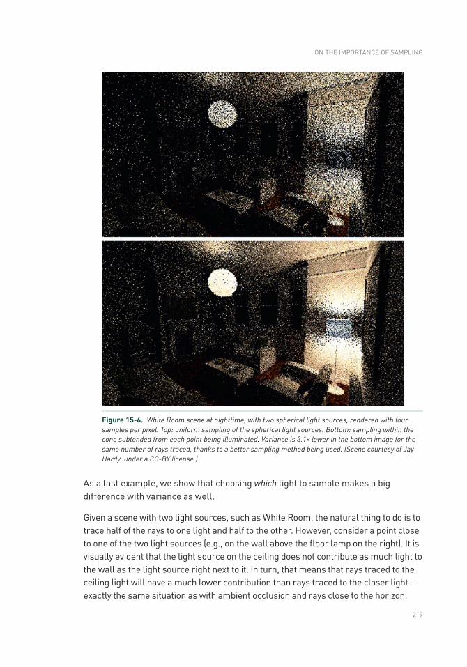
219
As a last example, we show that choosing which light to sample makes a big difference with variance as well.
Given a scene with two light sources, such as White Room, the natural thing to do is to trace half of the rays to one light and half to the other. However, consider a point close to one of the two light sources (e.g., on the wall above the floor lamp on the right). It is visually evident that the light source on the ceiling does not contribute as much light to the wall as the light source right next to it. In turn, that means that rays traced to the ceiling light will have a much lower contribution than rays traced to the closer light—exactly the same situation as with ambient occlusion and rays close to the horizon.
Figure 15-6. White Room scene at nighttime, with two spherical light sources, rendered with four samples per pixel. Top: uniform sampling of the spherical light sources. Bottom: sampling within the cone subtended from each point being illuminated. Variance is 3.1× lower in the bottom image for the same number of rays traced, thanks to a better sampling method being used. (Scene courtesy of Jay Hardy, under a CC-BY license.)
ON THE IMPORTANCE OF SAMPLING
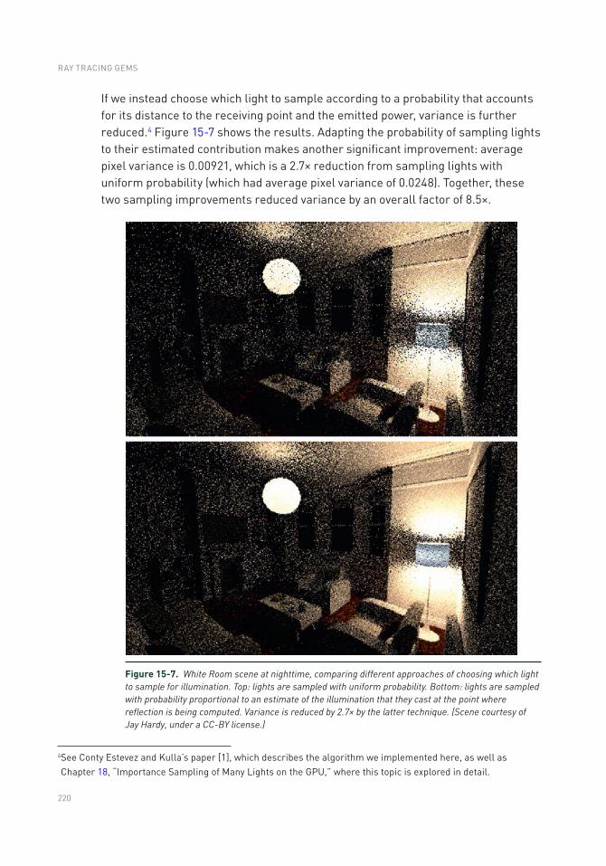
220
If we instead choose which light to sample according to a probability that accounts for its distance to the receiving point and the emitted power, variance is further reduced.4 Figure 15-7 shows the results. Adapting the probability of sampling lights to their estimated contribution makes another significant improvement: average pixel variance is 0.00921, which is a 2.7× reduction from sampling lights with uniform probability (which had average pixel variance of 0.0248). Together, these two sampling improvements reduced variance by an overall factor of 8.5×.
4 See Conty Estevez and Kulla’s paper [1], which describes the algorithm we implemented here, as well as Chapter 18, “Importance Sampling of Many Lights on the GPU,” where this topic is explored in detail.
Figure 15-7. White Room scene at nighttime, comparing different approaches of choosing which light to sample for illumination. Top: lights are sampled with uniform probability. Bottom: lights are sampled with probability proportional to an estimate of the illumination that they cast at the point where reflection is being computed. Variance is reduced by 2.7× by the latter technique. (Scene courtesy of Jay Hardy, under a CC-BY license.)
RAY TRACING GEMS
221
15.5 CONCLUSION
We hope that this chapter has left the reader with a basic understanding of the importance of the details of sampling and, more importantly, an understanding of why it is worth sampling well. It is easy to sample inefficiently, but it is not that much harder to sample well. We showed instances of reductions in variance by factors ranging from nearly 2× to 8.5×, purely thanks to more careful sampling and tracing more useful rays.
Given the connection between variance and sample count, another way to look at these results is that if you do not sample well, it is more or less the same as having a
GPU that is running at 12
to 18
of the actual performance it offers!
This chapter only scratched the surface of how to sample well in ray tracing; for example, we did not discussed how to sample according to the distributions defined by BSDFs or how to apply multiple importance sampling, an important variance reduction technique. See Chapter 28, “Ray Tracing Inhomogeneous Volumes”; Chapter 18, “Importance Sampling of Many Lights on the GPU”; and Chapter 16, “Sampling Transformations Zoo,” in this volume for more information on these topics. Furthermore, we did not discuss the substantial error reduction that can be achieved from using more uniformly distributed samples; see Keller’s survey [2] for more information about one such approach. Another useful resource for all these topics is the book Physically Based Rendering [4], which is now freely available in an online edition.
REFERENCES
[1] Conty Estevez, A., and Kulla, C. Importance Sampling of Many Lights with Adaptive Tree Splitting. Proceedings of the ACM on Computer Graphics and Interactive Techniques 1, 2 (2018), 25:1–25:17.
[2] Keller, A. Quasi-Monte Carlo Image Synthesis in a Nutshell. In Monte Carlo and Quasi-Monte Carlo Methods 2012. Springer, 2013, pp. 213–249.
[3] Kirk, D., and Arvo, J. Unbiased Sampling Techniques for Image Synthesis. Computer Graphics (SIGGRAPH) 25, 4 (1991), 153–156.
[4] Pharr, M., Jakob, W., and Humphreys, G. Physically Based Rendering: From Theory to Implementation, third ed. Morgan Kaufmann, 2016.
[5] Sobol, I. M. A Primer for the Monte Carlo Method. CRC Press, 1994.
[6] Veach, E., and Guibas, L. J. Optimally Combining Sampling Techniques for Monte Carlo Rendering. In Proceedings of SIGGRAPH (1995), pp. 419–428.
ON THE IMPORTANCE OF SAMPLING

222
Open Access This chapter is licensed under the terms of the Creative Commons Attribution-NonCommercial-NoDerivatives 4.0 International License (http://creativecommons.org/licenses/by-nc-nd/4.0/), which permits any noncommercial use, sharing, distribution and
reproduction in any medium or format, as long as you give appropriate credit to the original author(s) and the source, provide a link to the Creative Commons license and indicate if you modified the licensed material. You do not have permission under this license to share adapted material derived from this chapter or parts of it.
The images or other third party material in this chapter are included in the chapter's Creative Commons license, unless indicated otherwise in a credit line to the material. If material is not included in the chapter's Creative Commons license and your intended use is not permitted by statutory regulation or exceeds the permitted use, you will need to obtain permission directly from the copyright holder.
RAY TRACING GEMS
223© NVIDIA 2019 E. Haines, T. Akenine-Möller (eds.), Ray Tracing Gems, https://doi.org/10.1007/978-1-4842-4427-2_16
CHAPTER 16
Sampling Transformations ZooPeter Shirley, Samuli Laine, David Hart, Matt Pharr, Petrik Clarberg, Eric Haines, Matthias Raab, and David ClineNVIDIA
ABSTRACT
We present several formulas and methods for generating samples distributed according to a desired probability density function on a specific domain. Sampling is a fundamental operation in modern rendering, both at runtime and in preprocessing. It is becoming ever more prevalent with the introduction of ray tracing in standard APIs, as many ray tracing algorithms are based on sampling by nature. This chapter provides a concise list of some useful tricks and methods.
16.1 THE MECHANICS OF SAMPLING
A common task in ray tracing programs is to choose a set of samples on some domain with an underlying probability density function (PDF): for example, a set of points on the unit hemisphere whose probability density is proportional to the cosine of the polar angle. This is often accomplished by taking a set of samples that are uniform on the unit hypercube and transforming them to the desired domain. For readers unfamiliar with this general sample-generation pipeline, please refer to Chapter 13 of Pharr et al. [8].
This chapter catalogs a variety of methods to generate specific distributions that the authors have found useful in ray tracing programs. These are all either previously published or are part of the “conventional wisdom.”
224
16.2 INTRODUCTION TO DISTRIBUTIONS
In one dimension, there is a fairly standard way to create a transform that will generate samples with the desired PDF p. The key observation behind this method uses a construct called the cumulative distribution function (CDF), usually denoted with a capital P(x):
( ) ( )x
P x u x p y dyprobability distributed sathat aunifo mple .rmly ò-¥
= < = (1)
To see how this function can become useful, suppose that we want to determine where a particular uniformly distributed value u = 0.5 will go when passed through our desired warping function g : x = g(0.5). If we assume that g is nondecreasing (so its derivative is never negative), then half of the points will map to values of x less than g(0.5) and the other half to values of x greater than g(0.5). Because of the intrinsic property of CDFs, when P(x) = 0.5 we also know that half of the area under the PDF is to the left of that x, so we can deduce that
( )( )P g 0.5 0.5.= (2)
This basic observation actually works for any x in addition to x = 0.5. Thus, we have
( ) ( )g x P x1 ,-= (3)
where P−1 is the inverse function of P. The notation of inverse functions can be confusing. In practice what it means algebraically is that given a PDF p we integrate it using the integral in Equation 1, and then we solve for x in the resulting equation (which is inverting P):
( )u P x .=
Given a sequence of uniformly distributed samples u, we compute the inverse of P to find a p-distributed sequence of samples x.
For two-dimensional domains, two uniformly distributed samples are needed, u[0] and u[1]. These together give a point on the two-dimensional unit square: (u[0], u[1]) ∈ [0, 1)2. They can also be transformed to a desired domain.
RAY TRACING GEMS
225
For example, to pick a uniformly distributed sample on a unit disk, we would write down an integral in polar coordinates with a measure dA = rdrdφ, where r represents a distance (radius) from the origin along the angle φ from the positive x-axis. When possible in 2D domains, the two dimensions are separated into two independent 1D PDFs, and terms such as the r in the measure need to be handled
carefully. Although a uniform ( )jp
=p r, 1 for uniform density on the unit disk,
when separated into two 1D independent densities, the r is attached to the density of the radius. The resulting two 1D PDFs are
( ) ( )p p r r1 2
1 , 2 .2
jp
= = (4)
The constant terms 12p
and 2 make each of the PDFs integrate to 1 (a required
property of PDFs as discussed earlier). If we find the CDFs for those two PDFs, we get
( ) ( )P P r r 21 2, .
2jjp
= = (5)
If we want to transform uniform samples u[0] and u[1] to respect those CDFs, we can apply Equation 2 to each 1D CDF:
( )u u r 2[0], [1] , ,2jp
æ ö= ç ÷è ø
(6)
and then solve each for φ and r, yielding
( ) ( )j p=,r u , u2 [0] [1] . (7)
This basic “playbook” is used for most of the transforms found in the literature.
An important note is that, while our treatment assumes that (u[0], u[1]) are uniform on a unit square, in a higher-dimension d the points are uniformly distributed in the unit hypercube [0, 1)d. Such samples can be generated by (pseudo-)random or quasi-random methods [6].
The rest of this chapter gives several transforms, usually without derivation and most of them in two dimensions, that we have found to be useful in ray tracing programs.
SAMPLING TRANSFORMATIONS ZOO
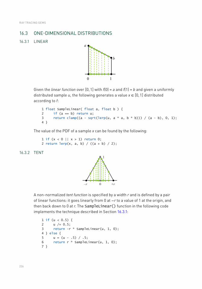
226
16.3 ONE-DIMENSIONAL DISTRIBUTIONS
16.3.1 LINEAR
Given the linear function over [0, 1] with f(0) = a and f(1) = b and given a uniformly distributed sample u, the following generates a value x ∈ [0, 1] distributed according to f:
1 float SampleLinear( float a, float b )
2 if (a == b) return u;
3 return clamp((a - sqrt(lerp(u, a * a, b * b))) / (a - b), 0, 1);
4
The value of the PDF of a sample x can be found by the following:
1 if (x < 0 || x > 1) return 0;
2 return lerp(x, a, b) / ((a + b) / 2);
16.3.2 TENT
A non-normalized tent function is specified by a width r and is defined by a pair of linear functions: it goes linearly from 0 at −r to a value of 1 at the origin, and then back down to 0 at r. The SampleLinear() function in the following code implements the technique described in Section 16.3.1:
1 if (u < 0.5)
2 u /= 0.5;
3 return -r * SampleLinear(u, 1, 0);
4 else
5 u = (u - .5) / .5;
6 return r * SampleLinear(u, 1, 0);
7
RAY TRACING GEMS
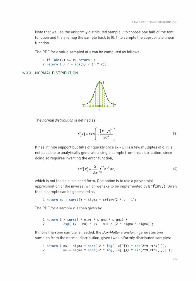
227
Note that we use the uniformly distributed sample u to choose one half of the tent function and then remap the sample back to [0, 1) to sample the appropriate linear function.
The PDF for a value sampled at x can be computed as follows:
1 if (abs(x) >= r) return 0;
2 return 1 / r - abs(x) / (r * r);
16.3.3 NORMAL DISTRIBUTION
The normal distribution is defined as
( ) ( )xf x
2
2exp .
2
m
s
æ ö-ç ÷= -ç ÷è ø
(8)
It has infinite support but falls off quickly once ‖ x − μ‖ is a few multiples of σ. It is not possible to analytically generate a single sample from this distribution, since doing so requires inverting the error function,
( )pò -=
x xx e dx2
0
2erf , (9)
which is not feasible in closed form. One option is to use a polynomial approximation of the inverse, which we take to be implemented by ErfInv(). Given that, a sample can be generated as
1 return mu + sqrt(2) * sigma * ErfInv(2 * u - 1);
The PDF for a sample x is then given by
1 return 1 / sqrt(2 * M_PI * sigma * sigma) *
2 exp(-(x - mu) * (x - mu) / (2 * sigma * sigma));
If more than one sample is needed, the Box-Müller transform generates two samples from the normal distribution, given two uniformly distributed samples:
1 return mu + sigma * sqrt(-2 * log(1-u[0])) * cos(2*M_PI*u[1]),
2 mu + sigma * sqrt(-2 * log(1-u[0])) * sin(2*M_PI*u[1])) ;
SAMPLING TRANSFORMATIONS ZOO
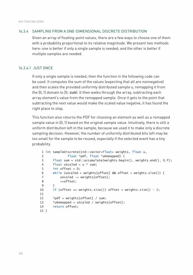
228
16.3.4 SAMPLING FROM A ONE-DIMENSIONAL DISCRETE DISTRIBUTION
Given an array of floating-point values, there are a few ways to choose one of them with a probability proportional to its relative magnitude. We present two methods here: one is better if only a single sample is needed, and the other is better if multiple samples are needed.
16.3.4.1 JUST ONCE
If only a single sample is needed, then the function in the following code can be used. It computes the sum of the values (expecting that all are nonnegative) and then scales the provided uniformly distributed sample u, remapping it from the [0, 1) domain to [0; sum). It then walks through the array, subtracting each array element’s value from the remapped sample. Once it gets to the point that subtracting the next value would make the scaled value negative, it has found the right place to stop.
This function also returns the PDF for choosing an element as well as a remapped sample value in [0, 1) based on the original sample value. Intuitively, there is still a uniform distribution left in the sample, because we used it to make only a discrete sampling decision. However, the number of uniformly distributed bits left may be too small for the sample to be reused, especially if the selected event has a tiny probability.
1 int SampleDiscrete(std::vector<float> weights, float u,
2 float *pdf, float *uRemapped)
3 float sum = std::accumulate(weights.begin(), weights.end(), 0.f);
4 float uScaled = u * sum;
5 int offset = 0;
6 while (uScaled > weights[offset] && offset < weights.size())
7 uScaled -= weights[offset];
8 ++offset;
9
10 if (offset == weights.size()) offset = weights.size() - 1;
11
12 *pdf = weights[offset] / sum;
13 *uRemapped = uScaled / weights[offset];
14 return offset;
15
RAY TRACING GEMS
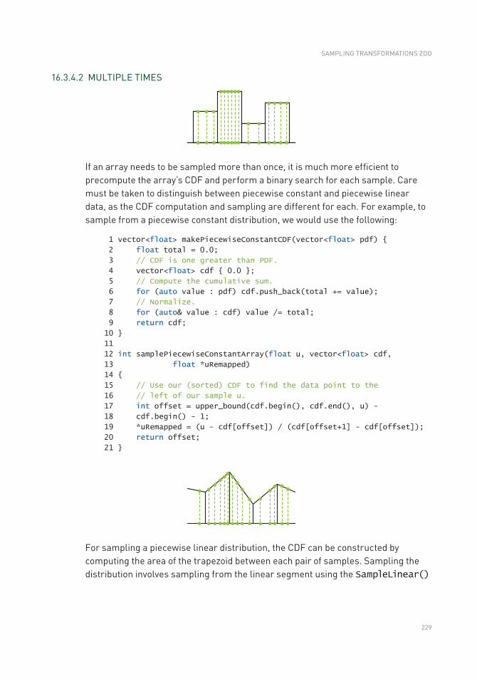
229
16.3.4.2 MULTIPLE TIMES
If an array needs to be sampled more than once, it is much more efficient to precompute the array’s CDF and perform a binary search for each sample. Care must be taken to distinguish between piecewise constant and piecewise linear data, as the CDF computation and sampling are different for each. For example, to sample from a piecewise constant distribution, we would use the following:
1 vector<float> makePiecewiseConstantCDF(vector<float> pdf)
2 float total = 0.0;
3 // CDF is one greater than PDF.
4 vector<float> cdf 0.0 ;
5 // Compute the cumulative sum.
6 for (auto value : pdf) cdf.push_back(total += value);
7 // Normalize.
8 for (auto& value : cdf) value /= total;
9 return cdf;
10
11
12 int samplePiecewiseConstantArray(float u, vector<float> cdf,
13 float *uRemapped)
14
15 // Use our (sorted) CDF to find the data point to the
16 // left of our sample u.
17 int offset = upper_bound(cdf.begin(), cdf.end(), u) -
18 cdf.begin() - 1;
19 *uRemapped = (u - cdf[offset]) / (cdf[offset+1] - cdf[offset]);
20 return offset;
21
For sampling a piecewise linear distribution, the CDF can be constructed by computing the area of the trapezoid between each pair of samples. Sampling the distribution involves sampling from the linear segment using the SampleLinear()
SAMPLING TRANSFORMATIONS ZOO
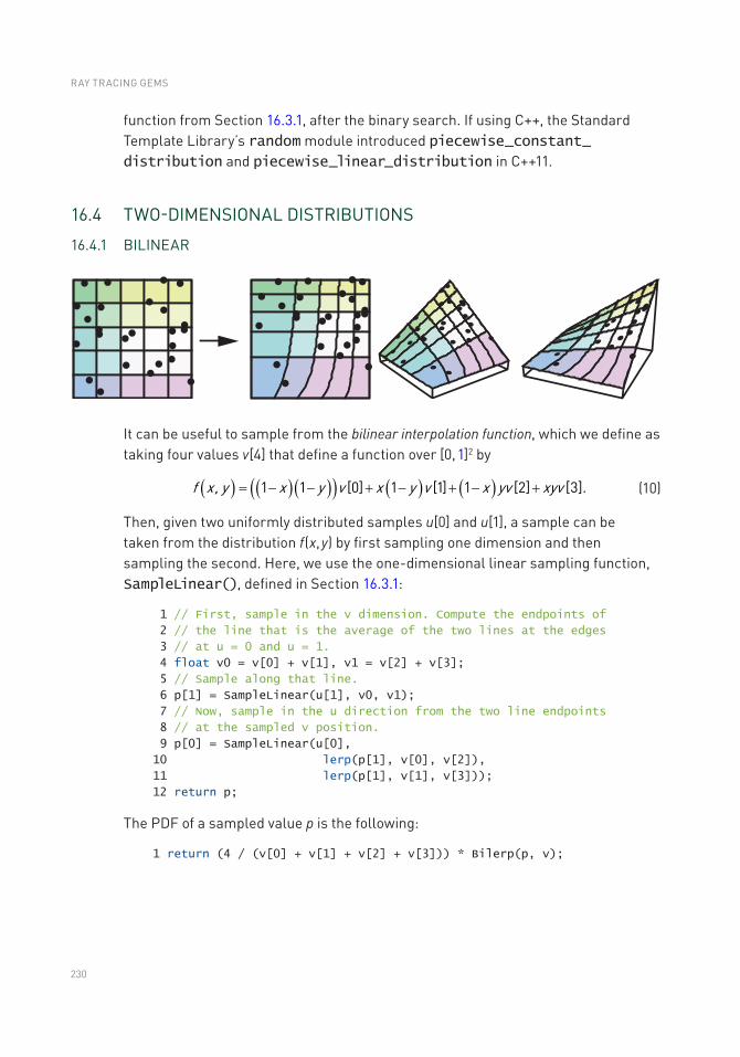
230
function from Section 16.3.1, after the binary search. If using C++, the Standard Template Library’s random module introduced piecewise_constant_distribution and piecewise_linear_distribution in C++11.
16.4 TWO-DIMENSIONAL DISTRIBUTIONS
16.4.1 BILINEAR
It can be useful to sample from the bilinear interpolation function, which we define as taking four values v[4] that define a function over [0, 1]2 by
( ) ( )( )( ) ( ) ( )f x, y x y v x y v x yv xyv1 1 [0] 1 [1] 1 [2] [3].= - - + - + - + (10)
Then, given two uniformly distributed samples u[0] and u[1], a sample can be taken from the distribution f(x, y) by first sampling one dimension and then sampling the second. Here, we use the one-dimensional linear sampling function, SampleLinear(), defined in Section 16.3.1:
1 // First, sample in the v dimension. Compute the endpoints of
2 // the line that is the average of the two lines at the edges
3 // at u = 0 and u = 1.
4 float v0 = v[0] + v[1], v1 = v[2] + v[3];
5 // Sample along that line.
6 p[1] = SampleLinear(u[1], v0, v1);
7 // Now, sample in the u direction from the two line endpoints
8 // at the sampled v position.
9 p[0] = SampleLinear(u[0],
10 lerp(p[1], v[0], v[2]),
11 lerp(p[1], v[1], v[3]));
12 return p;
The PDF of a sampled value p is the following:
1 return (4 / (v[0] + v[1] + v[2] + v[3])) * Bilerp(p, v);
RAY TRACING GEMS
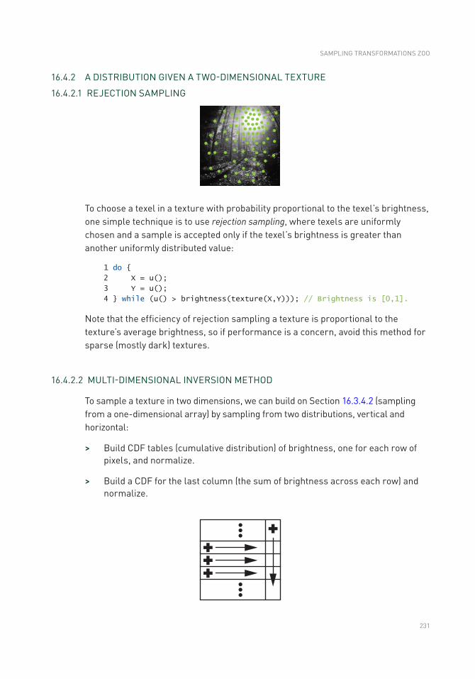
231
16.4.2 A DISTRIBUTION GIVEN A TWO-DIMENSIONAL TEXTURE
16.4.2.1 REJECTION SAMPLING
To choose a texel in a texture with probability proportional to the texel’s brightness, one simple technique is to use rejection sampling, where texels are uniformly chosen and a sample is accepted only if the texel’s brightness is greater than another uniformly distributed value:
1 do
2 X = u();
3 Y = u();
4 while (u() > brightness(texture(X,Y))); // Brightness is [0,1].
Note that the efficiency of rejection sampling a texture is proportional to the texture’s average brightness, so if performance is a concern, avoid this method for sparse (mostly dark) textures.
16.4.2.2 MULTI-DIMENSIONAL INVERSION METHOD
To sample a texture in two dimensions, we can build on Section 16.3.4.2 (sampling from a one-dimensional array) by sampling from two distributions, vertical and horizontal:
> Build CDF tables (cumulative distribution) of brightness, one for each row of pixels, and normalize.
> Build a CDF for the last column (the sum of brightness across each row) and normalize.
SAMPLING TRANSFORMATIONS ZOO
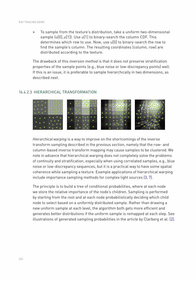
232
> To sample from the texture’s distribution, take a uniform two- dimensional sample (u[0], u[1]). Use u[1] to binary-search the column CDF. This determines which row to use. Now, use u[0] to binary-search the row to find the sample’s column. The resulting coordinates (column, row) are distributed according to the texture.
The drawback of this inversion method is that it does not preserve stratification properties of the sample points (e.g., blue noise or low-discrepancy points) well. If this is an issue, it is preferable to sample hierarchically in two dimensions, as described next.
16.4.2.3 HIERARCHICAL TRANSFORMATION
Hierarchical warping is a way to improve on the shortcomings of the inverse transform sampling described in the previous section, namely that the row- and column-based inverse transform mapping may cause samples to be clustered. We note in advance that hierarchical warping does not completely solve the problems of continuity and stratification, especially when using correlated samples, e.g., blue noise or low-discrepancy sequences, but it is a practical way to have some spatial coherence while sampling a texture. Example applications of hierarchical warping include importance sampling methods for complex light sources [3, 7].
The principle is to build a tree of conditional probabilities, where at each node we store the relative importance of the node’s children. Sampling is performed by starting from the root and at each node probabilistically deciding which child node to select based on a uniformly distributed sample. Rather than drawing a new uniform sample at each level, the algorithm both gets more efficient and generates better distributions if the uniform sample is remapped at each step. See illustrations of generated sampling probabilities in the article by Clarberg et al. [2].
RAY TRACING GEMS
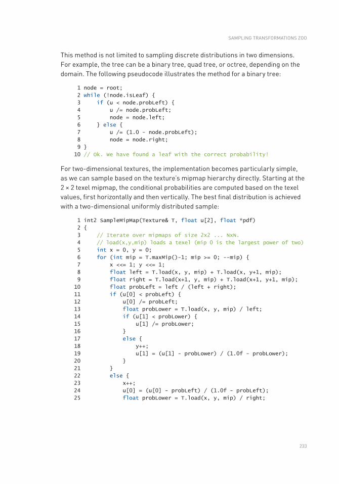
233
This method is not limited to sampling discrete distributions in two dimensions. For example, the tree can be a binary tree, quad tree, or octree, depending on the domain. The following pseudocode illustrates the method for a binary tree:
1 node = root;
2 while (!node.isLeaf)
3 if (u < node.probLeft)
4 u /= node.probLeft;
5 node = node.left;
6 else
7 u /= (1.0 - node.probLeft);
8 node = node.right;
9
10 // Ok. We have found a leaf with the correct probability!
For two-dimensional textures, the implementation becomes particularly simple, as we can sample based on the texture’s mipmap hierarchy directly. Starting at the 2 × 2 texel mipmap, the conditional probabilities are computed based on the texel values, first horizontally and then vertically. The best final distribution is achieved with a two-dimensional uniformly distributed sample:
1 int2 SampleMipMap(Texture& T, float u[2], float *pdf)
2
3 // Iterate over mipmaps of size 2x2 ... NxN.
4 // load(x,y,mip) loads a texel (mip 0 is the largest power of two)
5 int x = 0, y = 0;
6 for (int mip = T.maxMip()-1; mip >= 0; --mip)
7 x <<= 1; y <<= 1;
8 float left = T.load(x, y, mip) + T.load(x, y+1, mip);
9 float right = T.load(x+1, y, mip) + T.load(x+1, y+1, mip);
10 float probLeft = left / (left + right);
11 if (u[0] < probLeft)
12 u[0] /= probLeft;
13 float probLower = T.load(x, y, mip) / left;
14 if (u[1] < probLower)
15 u[1] /= probLower;
16
17 else
18 y++;
19 u[1] = (u[1] - probLower) / (1.0f - probLower);
20
21
22 else
23 x++;
24 u[0] = (u[0] - probLeft) / (1.0f - probLeft);
25 float probLower = T.load(x, y, mip) / right;
SAMPLING TRANSFORMATIONS ZOO
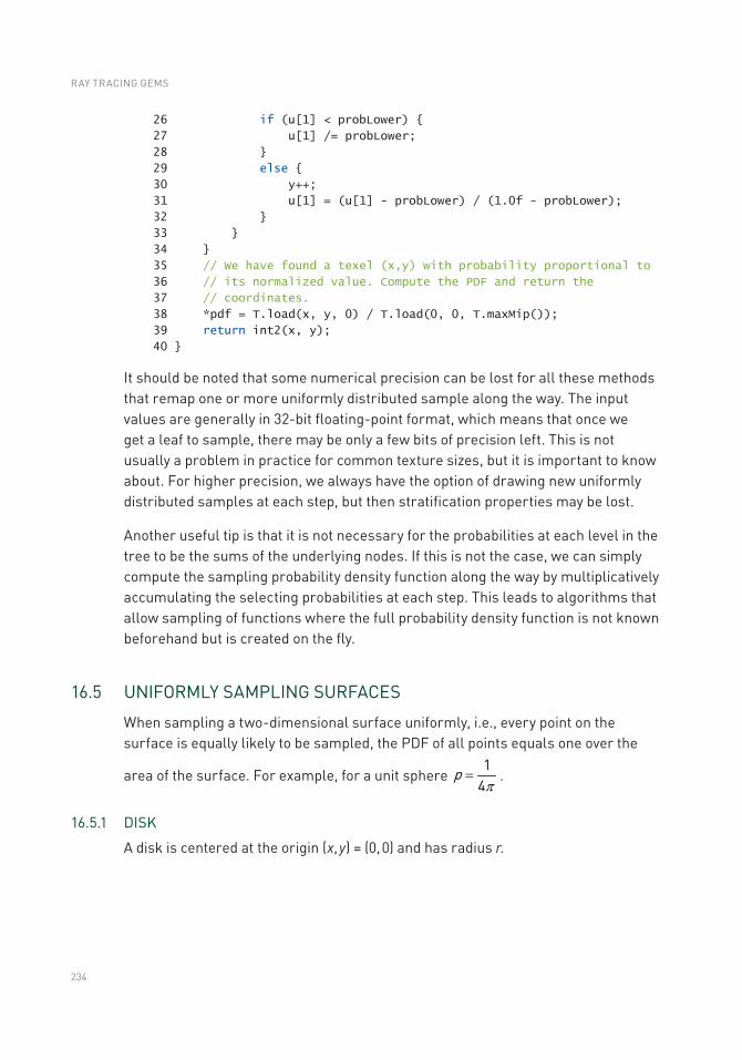
234
26 if (u[1] < probLower)
27 u[1] /= probLower;
28
29 else
30 y++;
31 u[1] = (u[1] - probLower) / (1.0f - probLower);
32
33
34
35 // We have found a texel (x,y) with probability proportional to
36 // its normalized value. Compute the PDF and return the
37 // coordinates.
38 *pdf = T.load(x, y, 0) / T.load(0, 0, T.maxMip());
39 return int2(x, y);
40
It should be noted that some numerical precision can be lost for all these methods that remap one or more uniformly distributed sample along the way. The input values are generally in 32-bit floating-point format, which means that once we get a leaf to sample, there may be only a few bits of precision left. This is not usually a problem in practice for common texture sizes, but it is important to know about. For higher precision, we always have the option of drawing new uniformly distributed samples at each step, but then stratification properties may be lost.
Another useful tip is that it is not necessary for the probabilities at each level in the tree to be the sums of the underlying nodes. If this is not the case, we can simply compute the sampling probability density function along the way by multiplicatively accumulating the selecting probabilities at each step. This leads to algorithms that allow sampling of functions where the full probability density function is not known beforehand but is created on the fly.
16.5 UNIFORMLY SAMPLING SURFACES
When sampling a two-dimensional surface uniformly, i.e., every point on the surface is equally likely to be sampled, the PDF of all points equals one over the
area of the surface. For example, for a unit sphere p 14p
= .
16.5.1 DISK
A disk is centered at the origin (x, y) = (0, 0) and has radius r.
RAY TRACING GEMS
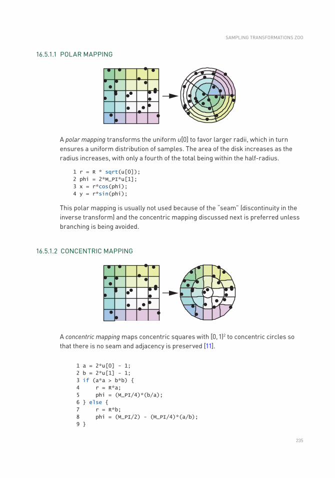
235
16.5.1.1 POLAR MAPPING
A polar mapping transforms the uniform u[0] to favor larger radii, which in turn ensures a uniform distribution of samples. The area of the disk increases as the radius increases, with only a fourth of the total being within the half-radius.
1 r = R * sqrt(u[0]);
2 phi = 2*M_PI*u[1];
3 x = r*cos(phi);
4 y = r*sin(phi);
This polar mapping is usually not used because of the “seam” (discontinuity in the inverse transform) and the concentric mapping discussed next is preferred unless branching is being avoided.
16.5.1.2 CONCENTRIC MAPPING
A concentric mapping maps concentric squares with [0, 1)2 to concentric circles so that there is no seam and adjacency is preserved [11].
1 a = 2*u[0] - 1;
2 b = 2*u[1] - 1;
3 if (a*a > b*b)
4 r = R*a;
5 phi = (M_PI/4)*(b/a);
6 else
7 r = R*b;
8 phi = (M_PI/2) - (M_PI/4)*(a/b);
9
SAMPLING TRANSFORMATIONS ZOO
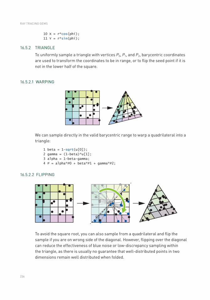
236
10 X = r*cos(phi);
11 Y = r*sin(phi);
16.5.2 TRIANGLE
To uniformly sample a triangle with vertices P0, P1, and P2, barycentric coordinates are used to transform the coordinates to be in range, or to flip the seed point if it is not in the lower half of the square.
16.5.2.1 WARPING
We can sample directly in the valid barycentric range to warp a quadrilateral into a triangle:
1 beta = 1-sqrt(u[0]);
2 gamma = (1-beta)*u[1];
3 alpha = 1-beta-gamma;
4 P = alpha*P0 + beta*P1 + gamma*P2;
16.5.2.2 FLIPPING
To avoid the square root, you can also sample from a quadrilateral and flip the sample if you are on wrong side of the diagonal. However, flipping over the diagonal can reduce the effectiveness of blue noise or low-discrepancy sampling within the triangle, as there is usually no guarantee that well-distributed points in two dimensions remain well distributed when folded.
RAY TRACING GEMS
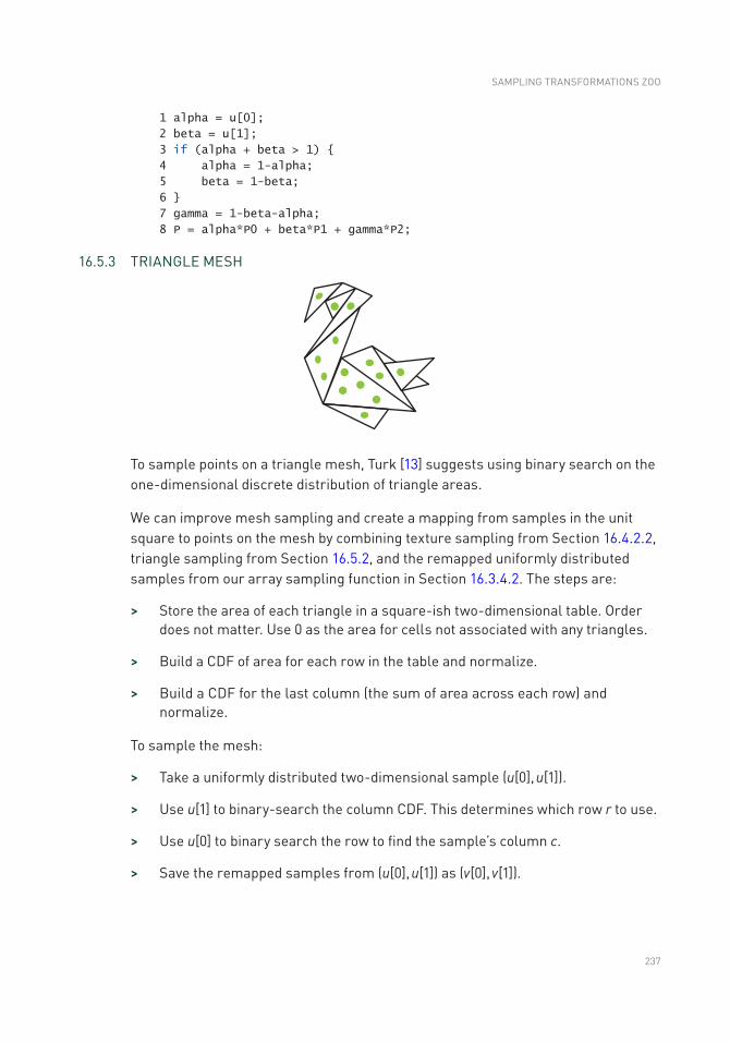
237
1 alpha = u[0];
2 beta = u[1];
3 if (alpha + beta > 1)
4 alpha = 1-alpha;
5 beta = 1-beta;
6
7 gamma = 1-beta-alpha;
8 P = alpha*P0 + beta*P1 + gamma*P2;
16.5.3 TRIANGLE MESH
To sample points on a triangle mesh, Turk [13] suggests using binary search on the one-dimensional discrete distribution of triangle areas.
We can improve mesh sampling and create a mapping from samples in the unit square to points on the mesh by combining texture sampling from Section 16.4.2.2, triangle sampling from Section 16.5.2, and the remapped uniformly distributed samples from our array sampling function in Section 16.3.4.2. The steps are:
> Store the area of each triangle in a square-ish two-dimensional table. Order does not matter. Use 0 as the area for cells not associated with any triangles.
> Build a CDF of area for each row in the table and normalize.
> Build a CDF for the last column (the sum of area across each row) and normalize.
To sample the mesh:
> Take a uniformly distributed two-dimensional sample (u[0], u[1]).
> Use u[1] to binary-search the column CDF. This determines which row r to use.
> Use u[0] to binary search the row to find the sample’s column c.
> Save the remapped samples from (u[0], u[1]) as (v[0], v[1]).
SAMPLING TRANSFORMATIONS ZOO
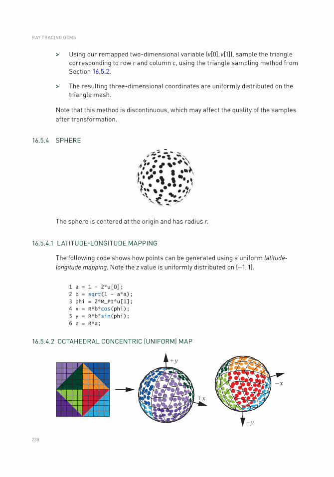
238
> Using our remapped two-dimensional variable (v[0], v[1]), sample the triangle corresponding to row r and column c, using the triangle sampling method from Section 16.5.2.
> The resulting three-dimensional coordinates are uniformly distributed on the triangle mesh.
Note that this method is discontinuous, which may affect the quality of the samples after transformation.
16.5.4 SPHERE
The sphere is centered at the origin and has radius r.
16.5.4.1 LATITUDE-LONGITUDE MAPPING
The following code shows how points can be generated using a uniform latitude-longitude mapping. Note the z value is uniformly distributed on (−1, 1].
1 a = 1 - 2*u[0];
2 b = sqrt(1 - a*a);
3 phi = 2*M_PI*u[1];
4 x = R*b*cos(phi);
5 y = R*b*sin(phi);
6 z = R*a;
16.5.4.2 OCTAHEDRAL CONCENTRIC (UNIFORM) MAP
RAY TRACING GEMS
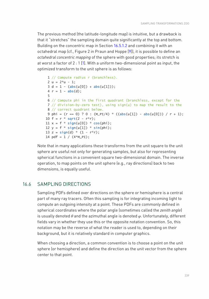
239
The previous method (the latitude-longitude map) is intuitive, but a drawback is that it “stretches” the sampling domain quite significantly at the top and bottom. Building on the concentric map in Section 16.5.1.2 and combining it with an octahedral map (cf., Figure 2 in Praun and Hoppe [9]), it is possible to define an octahedral concentric mapping of the sphere with good properties; its stretch is at worst a factor of 2 : 1 [1]. With a uniform two-dimensional point as input, the optimized transform to the unit sphere is as follows:
1 // Compute radius r (branchless).
2 u = 2*u - 1;
3 d = 1 - (abs(u[0]) + abs(u[1]));
4 r = 1 - abs(d);
5
6 // Compute phi in the first quadrant (branchless, except for the
7 // division-by-zero test), using sign(u) to map the result to the
8 // correct quadrant below.
9 phi = (r == 0) ? 0 : (M_PI/4) * ((abs(u[1]) - abs(u[0])) / r + 1);
10 f = r * sqrt(2 - r*r);
11 x = f * sign(u[0]) * cos(phi);
12 y = f * sign(u[1]) * sin(phi);
13 z = sign(d) * (1 - r*r);
14 pdf = 1 / (4*M_PI);
Note that in many applications these transforms from the unit square to the unit sphere are useful not only for generating samples, but also for representing spherical functions in a convenient square two-dimensional domain. The inverse operation, to map points on the unit sphere (e.g., ray directions) back to two dimensions, is equally useful.
16.6 SAMPLING DIRECTIONS
Sampling PDFs defined over directions on the sphere or hemisphere is a central part of many ray tracers. Often this sampling is for integrating incoming light to compute an outgoing intensity at a point. These PDFs are commonly defined in spherical coordinates where the polar angle (sometimes called the zenith angle) is usually denoted θ and the azimuthal angle is denoted φ. Unfortunately, different fields vary in whether they use this or the opposite notation convention. So, this notation may be the reverse of what the reader is used to, depending on their background, but it is relatively standard in computer graphics.
When choosing a direction, a common convention is to choose a point on the unit sphere (or hemisphere) and define the direction as the unit vector from the sphere center to that point.
SAMPLING TRANSFORMATIONS ZOO
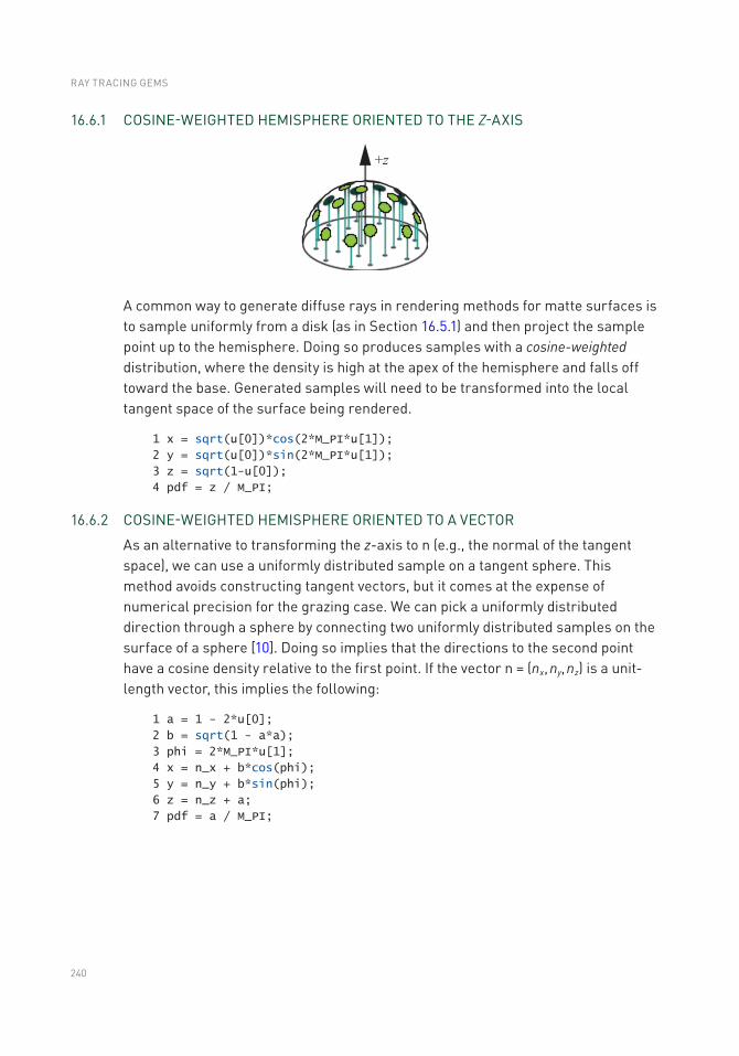
240
16.6.1 COSINE-WEIGHTED HEMISPHERE ORIENTED TO THE Z-AXIS
A common way to generate diffuse rays in rendering methods for matte surfaces is to sample uniformly from a disk (as in Section 16.5.1) and then project the sample point up to the hemisphere. Doing so produces samples with a cosine-weighted distribution, where the density is high at the apex of the hemisphere and falls off toward the base. Generated samples will need to be transformed into the local tangent space of the surface being rendered.
1 x = sqrt(u[0])*cos(2*M_PI*u[1]);
2 y = sqrt(u[0])*sin(2*M_PI*u[1]);
3 z = sqrt(1-u[0]);
4 pdf = z / M_PI;
16.6.2 COSINE-WEIGHTED HEMISPHERE ORIENTED TO A VECTOR
As an alternative to transforming the z-axis to n (e.g., the normal of the tangent space), we can use a uniformly distributed sample on a tangent sphere. This method avoids constructing tangent vectors, but it comes at the expense of numerical precision for the grazing case. We can pick a uniformly distributed direction through a sphere by connecting two uniformly distributed samples on the surface of a sphere [10]. Doing so implies that the directions to the second point have a cosine density relative to the first point. If the vector n = (nx, ny, nz) is a unit- length vector, this implies the following:
1 a = 1 - 2*u[0];
2 b = sqrt(1 - a*a);
3 phi = 2*M_PI*u[1];
4 x = n_x + b*cos(phi);
5 y = n_y + b*sin(phi);
6 z = n_z + a;
7 pdf = a / M_PI;
RAY TRACING GEMS
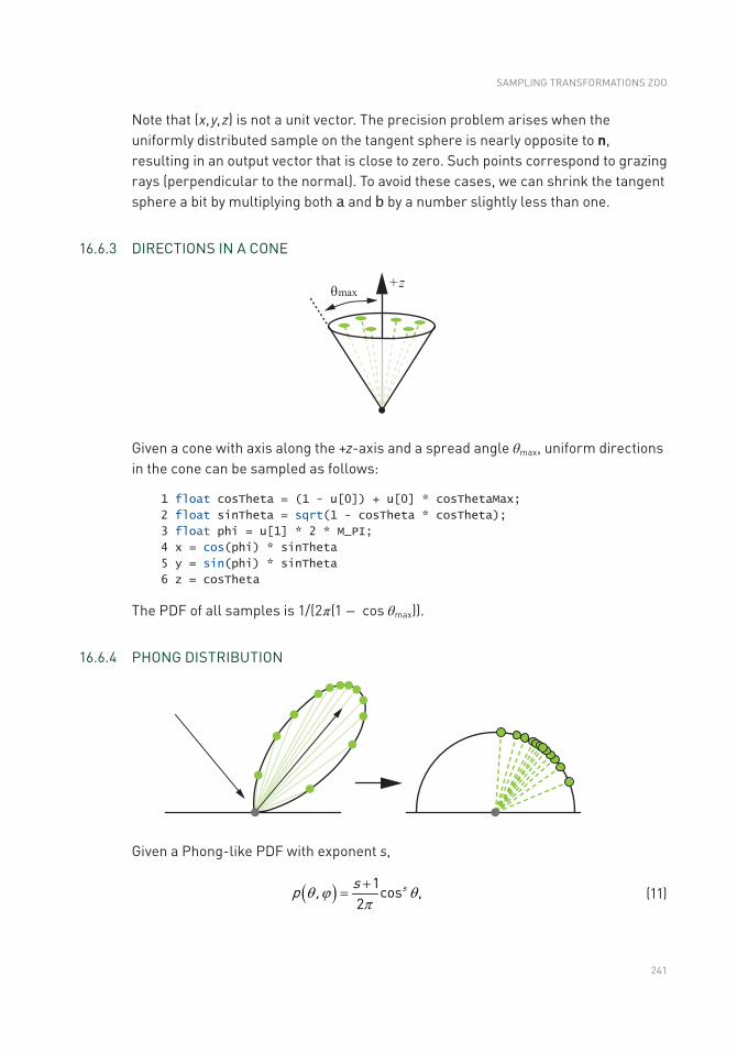
241
Note that (x, y, z) is not a unit vector. The precision problem arises when the uniformly distributed sample on the tangent sphere is nearly opposite to n, resulting in an output vector that is close to zero. Such points correspond to grazing rays (perpendicular to the normal). To avoid these cases, we can shrink the tangent sphere a bit by multiplying both a and b by a number slightly less than one.
16.6.3 DIRECTIONS IN A CONE
Given a cone with axis along the +z-axis and a spread angle θmax, uniform directions in the cone can be sampled as follows:
1 float cosTheta = (1 - u[0]) + u[0] * cosThetaMax;
2 float sinTheta = sqrt(1 - cosTheta * cosTheta);
3 float phi = u[1] * 2 * M_PI;
4 x = cos(phi) * sinTheta
5 y = sin(phi) * sinTheta
6 z = cosTheta
The PDF of all samples is 1/(2π(1 − cos θmax)).
16.6.4 PHONG DISTRIBUTION
Given a Phong-like PDF with exponent s,
( ) ssp , 1cos ,2
q j qp+
= (11)
SAMPLING TRANSFORMATIONS ZOO
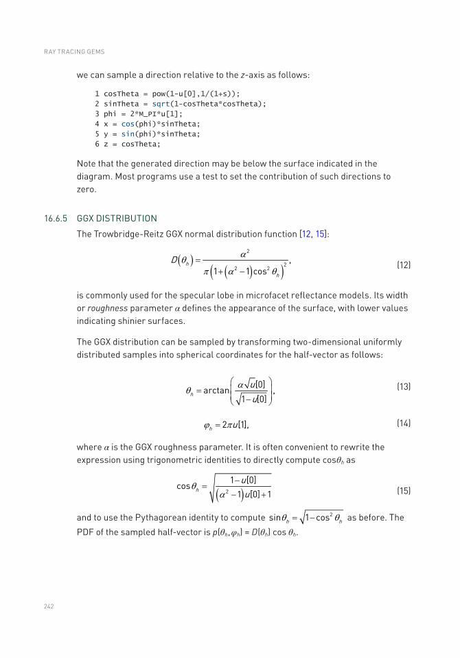
242
we can sample a direction relative to the z-axis as follows:
1 cosTheta = pow(1-u[0],1/(1+s));
2 sinTheta = sqrt(1-cosTheta*cosTheta);
3 phi = 2*M_PI*u[1];
4 x = cos(phi)*sinTheta;
5 y = sin(phi)*sinTheta;
6 z = cosTheta;
Note that the generated direction may be below the surface indicated in the diagram. Most programs use a test to set the contribution of such directions to zero.
16.6.5 GGX DISTRIBUTION
The Trowbridge-Reitz GGX normal distribution function [12, 15]:
( )( )( )
h
h
D2
22 2
,1 1 cos
aqp a q
=+ -
(12)
is commonly used for the specular lobe in microfacet reflectance models. Its width or roughness parameter α defines the appearance of the surface, with lower values indicating shinier surfaces.
The GGX distribution can be sampled by transforming two-dimensional uniformly distributed samples into spherical coordinates for the half-vector as follows:
h
uu[0]arctan ,
1 [0]
aqæ öç ÷=ç ÷-è ø
(13)
h u2 [1],j p= (14)
where α is the GGX roughness parameter. It is often convenient to rewrite the expression using trigonometric identities to directly compute cosθh as
( )huu2
1 [0]cos1 [0] 1
qa
-=
- + (15)
and to use the Pythagorean identity to compute h h2sin 1 cosq q= - as before. The
PDF of the sampled half-vector is p(θh, φh) = D(θh) cos θh.
RAY TRACING GEMS
243
For rendering, we are usually interested in sampling incident directions based on a given outgoing direction and local tangent frame. To do so, the outgoing direction v is reflected around the sampled half-vector h to find the incident direction as
( )ˆ ˆ ˆ2 ˆ ˆ= × -l v h h v . This operation changes the PDF above, which must be multiplied by
the Jacobian of the transform that is ( )( )1/ 4 ˆˆ ×v h in this case [14].
As with the Phong sampling in Section 16.6.4, the generated direction can be below the surface. Typically these are areas where the integrand is zero, but programmers should make sure to handle these cases carefully.
16.7 VOLUME SCATTERING
For volumes, also often called participating media, rays will “collide” with the volume in a probabilistic fashion. Some programs do this with incremental ray integration, but an alternative is to compute discrete collisions. For more information on volumes for graphics, see Chapter 11 of Pharr et al. [8].
Also see Chapter 28 for more information on this topic.
16.7.1 DISTANCES IN A VOLUME
Tracing photons through scattering and absorbing media requires importance sampling of distances proportional to the volume transmittance
( ) ( )kòæ ö= -ç ÷è ø
sT s t dt
0exp (16)
for the volume extinction coefficient κ(t). The PDF for this distribution is
( ) ( ) ( )k kòæ ö= -ç ÷è ø
sp s s t dt
0exp . (17)
16.7.1.1 HOMOGENEOUS MEDIA
In the case that κ is a constant, we have p(s) = κ exp (−sκ) and the inversion method can be used to obtain the following:
1 s = -log(1 - u) / kappa;
Note that 1 − u is important: remember that we assumed u ∈ [0, 1), so 1 − u ∈ (0, 1], which avoids invoking the logarithm for zero!
SAMPLING TRANSFORMATIONS ZOO
244
16.7.1.2 INHOMOGENEOUS MEDIA
For spatially varying κ(t), a procedure often referred to as Woodcock tracking gives the desired distribution [16]. Given the maximum extinction coefficient κmax along the ray and a generator u for samples uniform in [0, 1), the procedure is as follows:
1 s = 0;
2 do
3 s -= log(1 - u()) / kappa_max;
4 while (kappa(s) < u() * kappa_max);
16.7.2 HENYEY-GREENSTEIN PHASE FUNCTION
The Henyey-Greenstein phase function is a useful tool to model the directional scattering characteristics inside a volume. It is a PDF on the sphere of all directions that depends only on the angle θ between the incoming and outgoing directions and that is controlled with a single parameter g (the average cosine):
( )( )
gpg g
2
3/22
1 .4 1 2 cos
qp q
-=
+ - (18)
For g = 0 the scattering is isotropic, for g approaching −1 the scattering becomes highly focused forward scattering, and for g approaching 1 the scattering turns into highly focused backward scattering.
1 phi = 2.0 * M_PI * u[0];
2 if (g != 0)
3 tmp = (1 - g * g) / (1 + g * (1 - 2 * u[1]));
4 cos_theta = (1 + g * g - tmp * tmp) / (2 * g);
5 else
6 cos_theta = 1 - 2 * u[1];
7
16.8 ADDING TO THE ZOO COLLECTION
We have presented a variety of transforms we have found useful for ray tracing programs. We have not delved deeply into the theory needed to add to this collection. Readers that want to learn more about that theory so they can add their own “animals” can find thorough treatments in the books by Pharr et al. [8], Glassner [5], and Dutré et al. [4].
RAY TRACING GEMS
245
REFERENCES
[1] Clarberg, P. Fast Equal-Area Mapping of the (Hemi)Sphere Using SIMD. Journal of Graphics Tools 13, 3 (2008), 53–68.
[2] Clarberg, P., Jarosz, W., Akenine-Möller, T., and Jensen, H. W. Wavelet Importance Sampling: Efficiently Evaluating Products of Complex Functions. ACM Transactions on Graphics 24, 3 (2005), 1166–1175.
[3] Conty Estévez, A., and Kulla, C. Importance Sampling of Many Lights with Adaptive Tree Splitting. Proceedings of the ACM on Computer Graphics and Interactive Techniques 1, 2 (2018), 25:1–25:17.
[4] Dutré, P., Bekaert, P., and Bala, K. Advanced Global Illumination. A K Peters, 2006.
[5] Glassner, A. S. Principles of Digital Image Synthesis. Elsevier, 1995.
[6] Keller, A. Quasi-Monte Carlo Image Synthesis in a Nutshell. In Monte Carlo and Quasi-Monte Carlo Methods 2012. Springer, 2013, pp. 213–249.
[7] Keller, A., Wächter, C., Raab, M., Seibert, D., van Antwerpen, D., Korndörfer, J., and Kettner, L. The Iray Light Transport Simulation and Rendering System. arXiv, http://arxiv.org/abs/1705.01263, 2017.
[8] Pharr, M., Jakob, W., and Humphreys, G. Physically Based Rendering: From Theory to Implementation, third ed. Morgan Kaufmann, 2016.
[9] Praun, E., and Hoppe, H. Spherical Parametrization and Remeshing. ACM Transactions on Graphics 22, 3 (2003), 340–349.
[10] Sbert, M. An Integral Geometry Based Method for Fast Form-Factor Computation. Computer Graphics Forum 12, 3 (1993), 409–420.
[11] Shirley, P., and Chiu, K. A Low Distortion Map Between Disk and Square. Journal of Graphics Tools 2, 3 (1997), 45–52.
[12] Trowbridge, T. S., and Reitz, K. P. Average Irregularity Representation of a Rough Surface for Ray Reflection. Journal of the Optical Society of America 65, 5 (1975), 531–536.
[13] Turk, G. Generating Textures on Arbitrary Surfaces Using Reaction-Diffusion. Computer Graphics (SIGGRAPH) 25, 4 (July 1991), 289–298.
[14] Walter, B. Notes on the Ward BRDF. Tech. Rep. PCG-05-06, Cornell Program of Computer Graphics, April 2005.
[15] Walter, B., Marschner, S. R., Li, H., and Torrance, K. E. Microfacet Models for Refraction Through Rough Surfaces. In Proceedings of the 18th Eurographics Conference on Rendering Techniques (2007), pp. 195–206.
[16] Woodcock, E. R., Murphy, T., Hemmings, P. J., and Longworth, T. C. Techniques Used in the GEM Code for Monte Carlo Neutronics Calculations in Reactors and Other Systems of Complex Geometry. In Applications of Computing Methods to Reactor Problems (1965), p. 557.
SAMPLING TRANSFORMATIONS ZOO

246
Open Access This chapter is licensed under the terms of the Creative Commons Attribution-NonCommercial-NoDerivatives 4.0 International License (http://creativecommons.org/licenses/by-nc-nd/4.0/), which permits any noncommercial use, sharing, distribution and
reproduction in any medium or format, as long as you give appropriate credit to the original author(s) and the source, provide a link to the Creative Commons license and indicate if you modified the licensed material. You do not have permission under this license to share adapted material derived from this chapter or parts of it.
The images or other third party material in this chapter are included in the chapter's Creative Commons license, unless indicated otherwise in a credit line to the material. If material is not included in the chapter's Creative Commons license and your intended use is not permitted by statutory regulation or exceeds the permitted use, you will need to obtain permission directly from the copyright holder.
RAY TRACING GEMS
247© NVIDIA 2019 E. Haines, T. Akenine-Möller (eds.), Ray Tracing Gems, https://doi.org/10.1007/978-1-4842-4427-2_17
CHAPTER 17
Ignoring the Inconvenient When Tracing RaysMatt Pharr NVIDIA
ABSTRACT
Ray tracing’s greatest strength—that it can simulate all types of light transport—can also be its greatest weakness: when there are a few paths that unexpectedly carry much more light than others, the produced images contain a smattering of pixels that have bright spiky noise. Not only can it require a prohibitive number of additional rays to average out those spikes, but those pixels present a challenge for denoising algorithms. This chapter presents two techniques to address this problem, preventing it from occurring in the first place.
17.1 INTRODUCTION
Ray tracing is a marvelous algorithm, allowing unparalleled fidelity in the accurate simulation of light transport for image synthesis. No longer are rasterizer hacks required to generate high-quality images; real-time graphics programmers can now happily move forward to a new world, tracing rays to make beautiful images, and be free of the shackles of that history.
Now, let us move on to the new hacks.
17.2 MOTIVATION
Figure 17-1 presents two images of a pair of spheres in a box, both rendered with path tracing, using a few thousand paths per pixel to compute a high-quality reference image. The scene is illuminated by an area light source (not directly visible). The only difference between the two images is the material on the right-hand sphere: diffuse on the left and a perfectly specular mirror on the right.
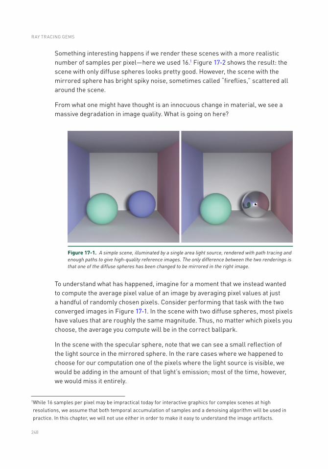
248
Something interesting happens if we render these scenes with a more realistic number of samples per pixel—here we used 16.1 Figure 17-2 shows the result: the scene with only diffuse spheres looks pretty good. However, the scene with the mirrored sphere has bright spiky noise, sometimes called “fireflies,” scattered all around the scene.
From what one might have thought is an innocuous change in material, we see a massive degradation in image quality. What is going on here?
To understand what has happened, imagine for a moment that we instead wanted to compute the average pixel value of an image by averaging pixel values at just a handful of randomly chosen pixels. Consider performing that task with the two converged images in Figure 17-1. In the scene with two diffuse spheres, most pixels have values that are roughly the same magnitude. Thus, no matter which pixels you choose, the average you compute will be in the correct ballpark.
In the scene with the specular sphere, note that we can see a small reflection of the light source in the mirrored sphere. In the rare cases where we happened to choose for our computation one of the pixels where the light source is visible, we would be adding in the amount of that light’s emission; most of the time, however, we would miss it entirely.
1 While 16 samples per pixel may be impractical today for interactive graphics for complex scenes at high resolutions, we assume that both temporal accumulation of samples and a denoising algorithm will be used in practice. In this chapter, we will not use either in order to make it easy to understand the image artifacts.
Figure 17-1. A simple scene, illuminated by a single area light source, rendered with path tracing and enough paths to give high-quality reference images. The only difference between the two renderings is that one of the diffuse spheres has been changed to be mirrored in the right image.
RAY TRACING GEMS
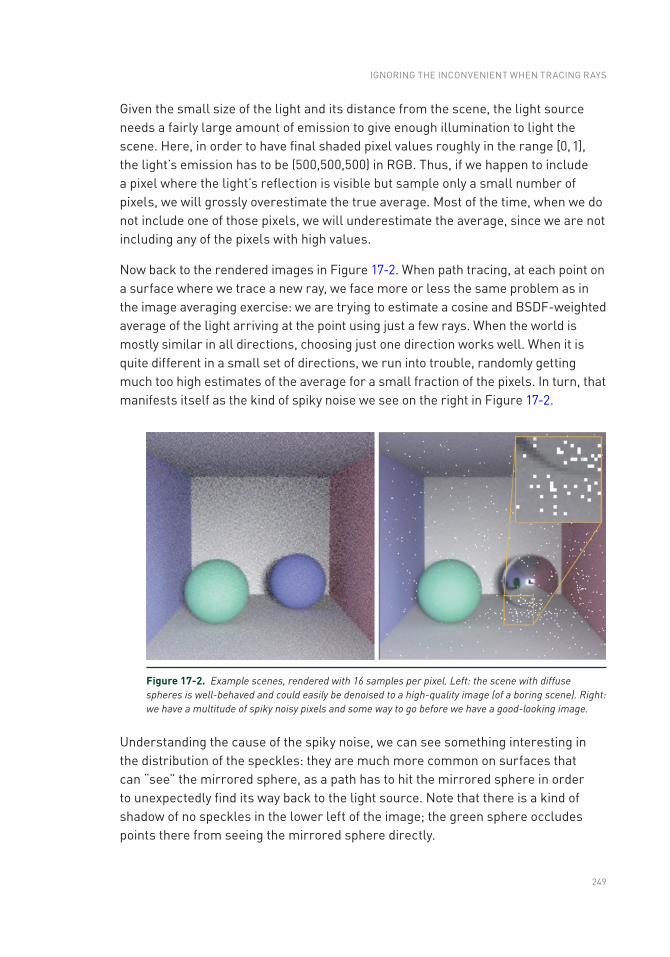
249
Given the small size of the light and its distance from the scene, the light source needs a fairly large amount of emission to give enough illumination to light the scene. Here, in order to have final shaded pixel values roughly in the range [0, 1], the light’s emission has to be (500,500,500) in RGB. Thus, if we happen to include a pixel where the light’s reflection is visible but sample only a small number of pixels, we will grossly overestimate the true average. Most of the time, when we do not include one of those pixels, we will underestimate the average, since we are not including any of the pixels with high values.
Now back to the rendered images in Figure 17-2. When path tracing, at each point on a surface where we trace a new ray, we face more or less the same problem as in the image averaging exercise: we are trying to estimate a cosine and BSDF-weighted average of the light arriving at the point using just a few rays. When the world is mostly similar in all directions, choosing just one direction works well. When it is quite different in a small set of directions, we run into trouble, randomly getting much too high estimates of the average for a small fraction of the pixels. In turn, that manifests itself as the kind of spiky noise we see on the right in Figure 17-2.
Figure 17-2. Example scenes, rendered with 16 samples per pixel. Left: the scene with diffuse spheres is well-behaved and could easily be denoised to a high-quality image (of a boring scene). Right: we have a multitude of spiky noisy pixels and some way to go before we have a good-looking image.
Understanding the cause of the spiky noise, we can see something interesting in the distribution of the speckles: they are much more common on surfaces that can “see” the mirrored sphere, as a path has to hit the mirrored sphere in order to unexpectedly find its way back to the light source. Note that there is a kind of shadow of no speckles in the lower left of the image; the green sphere occludes points there from seeing the mirrored sphere directly.
IGNORING THE INCONVENIENT WHEN TRACING RAYS
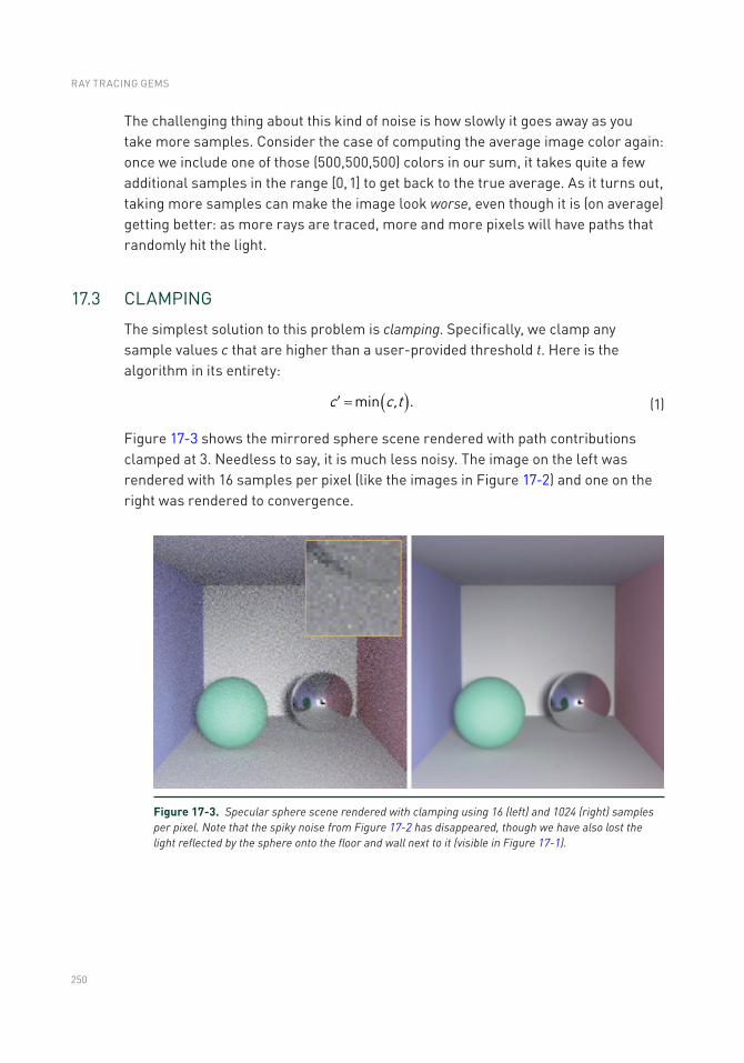
250
The challenging thing about this kind of noise is how slowly it goes away as you take more samples. Consider the case of computing the average image color again: once we include one of those (500,500,500) colors in our sum, it takes quite a few additional samples in the range [0, 1] to get back to the true average. As it turns out, taking more samples can make the image look worse, even though it is (on average) getting better: as more rays are traced, more and more pixels will have paths that randomly hit the light.
17.3 CLAMPING
The simplest solution to this problem is clamping. Specifically, we clamp any sample values c that are higher than a user-provided threshold t. Here is the algorithm in its entirety:
( )c c,tmin .¢ = (1)
Figure 17-3 shows the mirrored sphere scene rendered with path contributions clamped at 3. Needless to say, it is much less noisy. The image on the left was rendered with 16 samples per pixel (like the images in Figure 17-2) and one on the right was rendered to convergence.
Figure 17-3. Specular sphere scene rendered with clamping using 16 (left) and 1024 (right) samples per pixel. Note that the spiky noise from Figure 17-2 has disappeared, though we have also lost the light reflected by the sphere onto the floor and wall next to it (visible in Figure 17-1).
RAY TRACING GEMS
251
With 16 samples, the spiky noisy pixels are gone, and we are much closer to a good- looking image. However, note the difference between the 1024-sample image here and the final image in Figure 17-1: we have lost the focused light from the light source below the mirrored sphere on the floor and to the right on the wall (a so-called caustic). What is happening is that the illumination comes from a small number of high-contribution paths and, thus, clamping prevents them from contributing much to the final image.
17.4 PATH REGULARIZATION
Path regularization offers a less blunt hammer than clamping. It requires slightly more work to implement, but it does not suffer from the loss of energy that we saw with clamping.
Consider again the thought exercise of computing the average value of the image from just a few pixels: if you have an image with a few very bright pixels, like we have with the reflection of the light source in the mirrored sphere, then you could imagine that you would get a better result if you were able to apply a wide blur to the image before picking pixels to average. In that way, the bright pixels are both spread out and made dimmer, and thus the blurred image has less variation and which pixels you choose matters less.
Path regularization is based on this idea. The concept is straightforward: blur the BSDFs in the scene when they are encountered by indirect rays. When regularization is performed at such points, the sphere becomes glossy specular rather than perfectly specular.
The left image in Figure 17-4 shows how this works with our scene at 16 samples per pixel, and the right one shows its appearance as the image converges at around 128 samples. Regularization has eliminated the spiky noise while still preserving a representation of the caustic reflection of the light source.
IGNORING THE INCONVENIENT WHEN TRACING RAYS
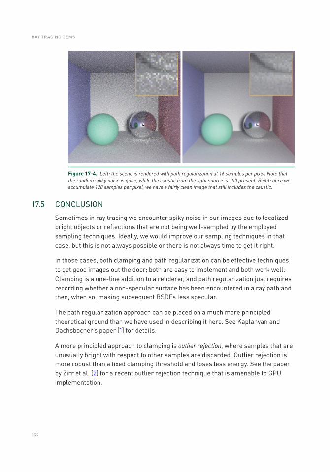
252
17.5 CONCLUSION
Sometimes in ray tracing we encounter spiky noise in our images due to localized bright objects or reflections that are not being well-sampled by the employed sampling techniques. Ideally, we would improve our sampling techniques in that case, but this is not always possible or there is not always time to get it right.
In those cases, both clamping and path regularization can be effective techniques to get good images out the door; both are easy to implement and both work well. Clamping is a one-line addition to a renderer, and path regularization just requires recording whether a non-specular surface has been encountered in a ray path and then, when so, making subsequent BSDFs less specular.
The path regularization approach can be placed on a much more principled theoretical ground than we have used in describing it here. See Kaplanyan and Dachsbacher’s paper [1] for details.
A more principled approach to clamping is outlier rejection, where samples that are unusually bright with respect to other samples are discarded. Outlier rejection is more robust than a fixed clamping threshold and loses less energy. See the paper by Zirr et al. [2] for a recent outlier rejection technique that is amenable to GPU implementation.
Figure 17-4. Left: the scene is rendered with path regularization at 16 samples per pixel. Note that the random spiky noise is gone, while the caustic from the light source is still present. Right: once we accumulate 128 samples per pixel, we have a fairly clean image that still includes the caustic.
RAY TRACING GEMS

253
REFERENCES
[1] Kaplanyan, A. S., and Dachsbacher, C. Path Space Regularization for Holistic and Robust Light Transport. Computer Graphics Forum 32, 2 (2013), 63–72.
[2] Zirr, T., Hanika, J., and Dachsbacher, C. Reweighting Firefly Samples for Improved Finite-Sample Monte Carlo Estimates. Computer Graphics Forum 37, 6 (2018), 410–421.
Open Access This chapter is licensed under the terms of the Creative Commons Attribution-NonCommercial-NoDerivatives 4.0 International License (http://creativecommons.org/licenses/by-nc-nd/4.0/), which permits any noncommercial use, sharing, distribution and
reproduction in any medium or format, as long as you give appropriate credit to the original author(s) and the source, provide a link to the Creative Commons license and indicate if you modified the licensed material. You do not have permission under this license to share adapted material derived from this chapter or parts of it.
The images or other third party material in this chapter are included in the chapter's Creative Commons license, unless indicated otherwise in a credit line to the material. If material is not included in the chapter's Creative Commons license and your intended use is not permitted by statutory regulation or exceeds the permitted use, you will need to obtain permission directly from the copyright holder.
IGNORING THE INCONVENIENT WHEN TRACING RAYS
255© NVIDIA 2019 E. Haines, T. Akenine-Möller (eds.), Ray Tracing Gems, https://doi.org/10.1007/978-1-4842-4427-2_18
CHAPTER 18
Importance Sampling of Many Lights on the GPUPierre Moreau1,2 and Petrik Clarberg1 1NVIDIA 2Lund University
ABSTRACT
The introduction of standardized APIs for ray tracing, together with hardware acceleration, opens up possibilities for physically based lighting in real-time rendering. Light importance sampling is one of the fundamental operations in light transport simulations, applicable to both direct and indirect illumination. This chapter describes a bounding volume hierarchy data structure and associated sampling methods to accelerate importance sampling of local light sources. The work is based on recently published methods for light sampling in production rendering, but it is evaluated in a real-time implementation using Microsoft DirectX Raytracing.
18.1 INTRODUCTION
A realistic scene may contain hundreds of thousands of light sources. The accurate simulation of the light and shadows that they cast is one of the most important factors for realism in computer graphics. Traditional real-time applications with rasterized shadow maps have been practically limited to use a handful of carefully selected dynamic lights. Ray tracing allows more flexibility, as we can trace shadow rays to different sampled lights at each pixel.
Mathematically speaking, the best way to select those samples is to pick lights with a probability in proportion to each light’s contribution. However, the contribution varies spatially and depends on the local surface properties and visibility. Hence, it is challenging to find a single global probability density function (PDF) that works well everywhere.
The solution that we explore in this chapter is to use a hierarchical acceleration structure built over the light sources to guide the sampling [11, 22]. Each node in the data structure represents a cluster of lights. The idea is to traverse the tree from top to bottom, at each level estimating how much each cluster
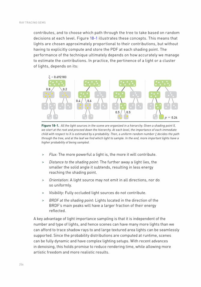
256
contributes, and to choose which path through the tree to take based on random decisions at each level. Figure 18-1 illustrates these concepts. This means that lights are chosen approximately proportional to their contributions, but without having to explicitly compute and store the PDF at each shading point. The performance of the technique ultimately depends on how accurately we manage to estimate the contributions. In practice, the pertinence of a light or a cluster of lights, depends on its:
> Flux: The more powerful a light is, the more it will contribute.
> Distance to the shading point: The further away a light lies, the smaller the solid angle it subtends, resulting in less energy reaching the shading point.
> Orientation: A light source may not emit in all directions, nor do so uniformly.
> Visibility: Fully occluded light sources do not contribute.
> BRDF at the shading point: Lights located in the direction of the BRDF’s main peaks will have a larger fraction of their energy reflected.
A key advantage of light importance sampling is that it is independent of the number and type of lights, and hence scenes can have many more lights than we can afford to trace shadow rays to and large textured area lights can be seamlessly supported. Since the probability distributions are computed at runtime, scenes can be fully dynamic and have complex lighting setups. With recent advances in denoising, this holds promise to reduce rendering time, while allowing more artistic freedom and more realistic results.
Figure 18-1. All the light sources in the scene are organized in a hierarchy. Given a shading point X, we start at the root and proceed down the hierarchy. At each level, the importance of each immediate child with respect to X is estimated by a probability. Then, a uniform random number ξ decides the path through the tree, and at the leaf we find which light to sample. In the end, more important lights have a higher probability of being sampled.
RAY TRACING GEMS
257
In the following, we discuss light importance sampling in more detail and present a real-time implementation that uses a bounding volume hierarchy (BVH) over the lights. The method is implemented using the Microsoft DirectX Raytracing (DXR) API, and source code is available.
18.2 REVIEW OF PREVIOUS ALGORITHMS
With the transition to path tracing in production rendering [21, 31], the visibility sampling is solved by tracing shadow rays toward sampled points on the light sources. When a shadow ray does not hit anything on its way from a shading point to the light, the point is deemed to be lit. By averaging over many such samples over the surfaces of the lights, a good approximation of the lighting is achieved. The approximation converges to ground truth as more samples are taken. However, with more than a handful of light sources, exhaustive sampling is not a viable strategy, not even in production rendering.
To handle the complexity of dynamic lighting with many lights, most techniques generally rely on building some form of spatial acceleration structure over the lights, which is then used to accelerate rendering by either culling, approximating, or importance-sampling the lights.
18.2.1 REAL-TIME LIGHT CULLING
Game engines have transitioned to use mostly physically based materials and light sources specified in physical units [19, 23]. However, for performance reasons and due to the limitations of the rasterization pipeline, only a few point-like light sources can be rendered in real time with shadow maps. The cost per light is high and the performance scales linearly with the number of lights. For area lights, the unshadowed contribution can be computed using linearly transformed cosines [17], but the problem of evaluating visibility remains.
To reduce the number of lights that need to be considered, it is common to artificially limit the influence region of individual lights, for example, by using an approximate quadratic falloff that goes to zero at some distance. By careful placement and tweaking of the light parameters, the number of lights that affect any given point can be limited.
Tiled shading [2, 28] works by binning such lights into screen-space tiles, where the depth bounds of the tiles effectively reduce the number of lights that need to be processed when shading each tile. Modern variants improve culling rates by splitting frusta in depth (2.5D culling) [15], by clustering shading points or lights [29, 30], or by using per-tile light trees [27].
IMPORTANCE SAMPLING OF MANy LIGHTS ON THE GPU
258
A drawback of these culling methods is that the acceleration structure is in screen space. Another drawback is that the required clamped light ranges can introduce noticeable darkening. This is particularly noticeable in cases where many dim lights add up to a significant contribution, such as Christmas tree lights or indoor office illumination. To address this, Tokuyoshi and Harada [40] propose using stochastic light ranges to randomly reject unimportant lights rather than assigning fixed ranges. They also show a proof-of-concept of the technique applied to path tracing using a bounding sphere hierarchy over the light sources.
18.2.2 MANy-LIGHT ALGORITHMS
Virtual point lights (VPLs) [20] have long been used to approximate global illumination. The idea is to trace photons from the light sources and deposit VPLs at path vertices, which are then used to approximate the indirect illumination. VPL methods are conceptually similar to importance sampling methods for many lights. The lights are clustered into nodes in a tree, and during traversal estimated contributions are computed. The main difference is that, for importance sampling, the estimations are used to compute light selection probabilities rather than directly to approximate the lighting.
For example, lightcuts [44, 45] accelerate the rendering with millions of VPLs by traversing the tree per shading point and computing error bounds on the estimated contributions. The algorithm chooses to use a cluster of VPLs directly as a light source, avoiding subdivision to finer clusters or individual VPLs, when the error is sufficiently small. We refer to the survey by Dachsbacher et al. [12] for a good overview of these and other many-light techniques. See also the overview of global illumination algorithms by Christensen and Jarosz [8].
18.2.3 LIGHT IMPORTANCE SAMPLING
In early work on accelerating ray tracing with many lights, the lights are sorted according to contribution and only the ones above a threshold are shadow tested [46]. The contribution of the remaining lights is then added based on a statistical estimate of their visibility.
Shirley et al. [37] describe importance sampling for various types of light sources. They classify lights as bright or dim by comparing their estimated contributions to a user-defined threshold. To sample from multiple lights, they use an octree that is hierarchically subdivided until the number of bright lights is sufficiently small. The contribution of an octree cell is estimated by evaluating the contribution at a large number of points on the cell’s boundary. Zimmerman and Shirley [47] use a uniform spatial subdivision instead and include an estimated visibility in the cells.
RAY TRACING GEMS
259
For real-time ray tracing with many lights, Schmittler et al. [36] restrict the influence region of lights and use a k-d tree to quickly locate the lights that affect each point. Bikker takes a similar approach in the Arauna ray tracer [5, 6], but it uses a BVH with spherical nodes to more tightly bound the light volumes. Shading is done Whitted- style by evaluating all contributing lights. These methods suffer from bias as the light contributions are cut off, but that may potentially be alleviated with stochastic light ranges as mentioned earlier [40].
In the Brigade real-time path tracer, Bikker [6] uses resampled importance sampling [39]. A first set of lights is selected based on a location-invariant probability density function, and then this set is resampled by more accurately estimating the contributions using the BRDF and distances to pick one important light. In this approach, there is no hierarchical data structure.
The Iray rendering system [22] uses a hierarchical light importance sampling scheme. Iray works with triangles exclusively and assigns a single flux (power) value per triangle. A BVH is built over the triangular lights and traversed probabilistically, at each node computing the estimated contribution of each subtree. The system encodes directional information at each node by dividing the unit sphere into a small number of regions and storing one representative flux value per region. Estimated flux from BVH nodes is computed based on the distance to the center of the node.
Conty Estevez and Kulla [11] take a similar approach for cinematic rendering. They use a 4-wide BVH that also includes analytic light shapes, and the lights are clustered in world space including orientation by using bounding cones. In the traversal, they probabilistically select which branch to traverse based on a single uniform random number. The number is rescaled to the unit range at each step, which preserves stratification properties (the same technique is used in hierarchical sample warping [9]). To reduce the problem of poor estimations for large nodes, they use a metric for adaptively splitting such nodes during traversal. Our real-time implementation is based on their technique, with some simplifications.
18.3 FOUNDATIONS
In this section, we will first review the foundations of physically based lighting and importance sampling, before diving into the technical details of our real-time implementation.
IMPORTANCE SAMPLING OF MANy LIGHTS ON THE GPU
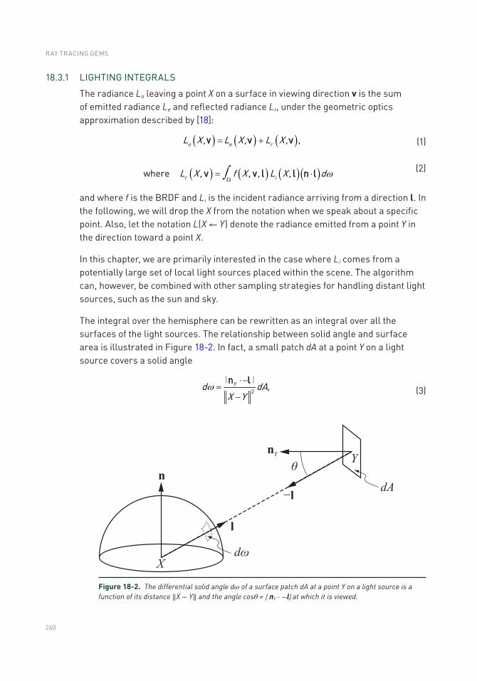
260
18.3.1 LIGHTING INTEGRALS
The radiance Lo leaving a point X on a surface in viewing direction v is the sum of emitted radiance Le and reflected radiance Lr, under the geometric optics approximation described by [18]:
( ) ( ) ( )o e rL X , L X , L X , ,= +v v v (1)
( ) ( ) ( )( )r iL X , f X , , L X , dwhere wòW= ×v v l l n l (2)
and where f is the BRDF and Li is the incident radiance arriving from a direction l. In the following, we will drop the X from the notation when we speak about a specific point. Also, let the notation L(X ← Y) denote the radiance emitted from a point Y in the direction toward a point X.
In this chapter, we are primarily interested in the case where Li comes from a potentially large set of local light sources placed within the scene. The algorithm can, however, be combined with other sampling strategies for handling distant light sources, such as the sun and sky.
The integral over the hemisphere can be rewritten as an integral over all the surfaces of the light sources. The relationship between solid angle and surface area is illustrated in Figure 18-2. In fact, a small patch dA at a point Y on a light source covers a solid angle
yd dA
X y2
,w×-
=-
n l∣ ∣ (3)
Figure 18-2. The differential solid angle dω of a surface patch dA at a point Y on a light source is a function of its distance ‖X − Y‖ and the angle cosθ = ∣ nY ⋅ −l∣ at which it is viewed.
RAY TRACING GEMS
261
i.e., there is an inverse square falloff by distance and a dot product between the light’s normal nY and the emitted light direction −l. Note that in our implementation, light sources may be single-sided or double-sided emitters. For single-sided lights, we set the emitted radiance L(X ← Y) = 0 if (nY ⋅ −l) ≤ 0.
We also need to know the visibility between our shading point X and the point Y on the light source, formally expressed as
( ) 1 if and are mutually visible,0 otherwise.
X yv X y
ì« = í
î (4)
In practice, we evaluate v by tracing shadow rays from X in direction l, with the ray’s maximum distance tmax = ‖ X − Y‖. Note that to avoid self-intersections due to numerical issues, the ray origin needs to be offset and the ray shortened slightly using epsilons. See Chapter 6 for details.
Now, assuming that there are m light sources in the scene, the reflected radiance in Equation 2 can be written as
( ) ( )m
r r ii
L X , L X ,,1
, where=
= åv v (5)
( ) ( ) ( ) ( ) ( ) yr i i iL X , f X , , L X y v X y , dA
X y, 2
max 0 .òW×-
= ¬ « ×-
n lv v l n l
∣ ∣ (6)
That is, Lr is the sum of the reflected light from each individual light i = 1, … , m. Note that we clamp n ⋅ l because light from points backfacing to the shading point cannot contribute. The complexity is linear in the number of lights m, which may become expensive when m is large. This leads us to the next topic.
18.3.2 IMPORTANCE SAMPLING
As discussed in Section 18.2, there are two fundamentally different ways to reduce the cost of Equation 5. One method is to limit the influence regions of lights, and thereby reduce m. The other method is to sample a small subset of lights n ≪ m. This can be done in such a way that the result is consistent, i.e., it converges to the ground truth as n grows.
IMPORTANCE SAMPLING OF MANy LIGHTS ON THE GPU
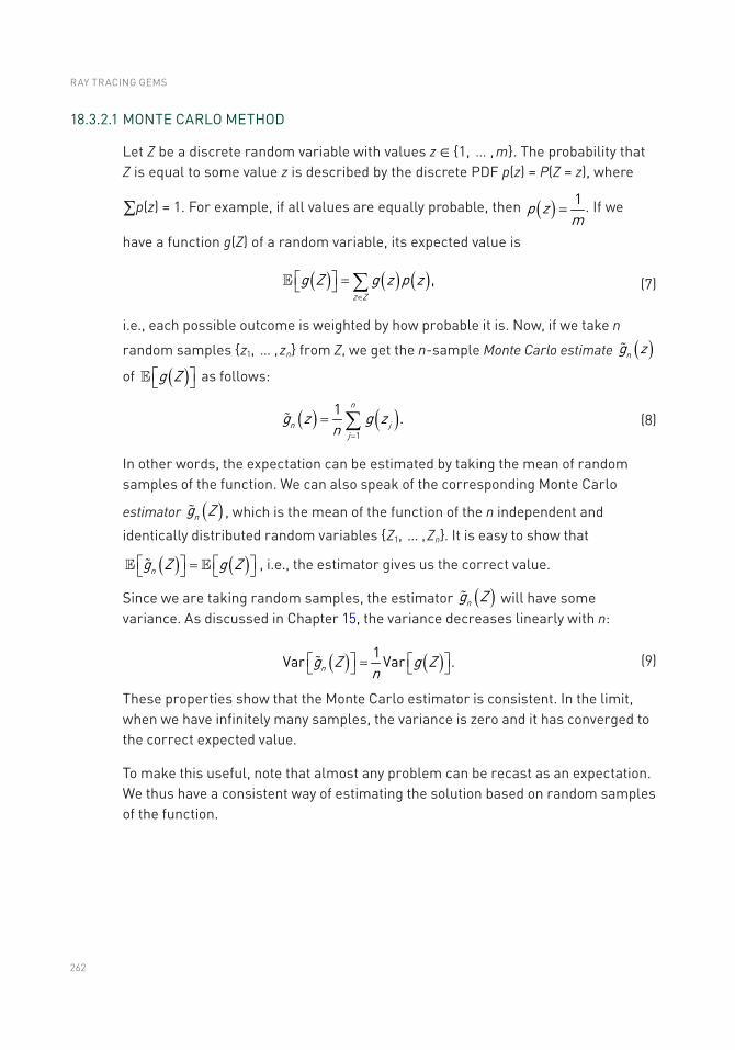
262
18.3.2.1 MONTE CARLO METHOD
Let Z be a discrete random variable with values z ∈ 1, … , m. The probability that Z is equal to some value z is described by the discrete PDF p(z) = P(Z = z), where
∑p(z) = 1. For example, if all values are equally probable, then ( )p zm1
= . If we
have a function g(Z) of a random variable, its expected value is
( ) ( ) ( )z Z
g Z g z p z ,Î
é ù =ë û å (7)
i.e., each possible outcome is weighted by how probable it is. Now, if we take n
random samples z1, … , zn from Z, we get the n-sample Monte Carlo estimate ( )ng z
of ( )g Zé ùë û as follows:
( ) ( )n
n jj
g z g zn 1
1 .=
= å (8)
In other words, the expectation can be estimated by taking the mean of random samples of the function. We can also speak of the corresponding Monte Carlo
estimator ( )ng Z , which is the mean of the function of the n independent and
identically distributed random variables Z1, … , Zn. It is easy to show that
( ) ( )ng Z g Zé ù é ù=ë û ë û , i.e., the estimator gives us the correct value.
Since we are taking random samples, the estimator ( )n Zg will have some variance. As discussed in Chapter 15, the variance decreases linearly with n:
( ) ( )n Z g Zn
g 1Var Var .é ù é ù=ë û ë û (9)
These properties show that the Monte Carlo estimator is consistent. In the limit, when we have infinitely many samples, the variance is zero and it has converged to the correct expected value.
To make this useful, note that almost any problem can be recast as an expectation. We thus have a consistent way of estimating the solution based on random samples of the function.
RAY TRACING GEMS
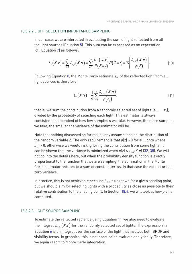
263
18.3.2.2 LIGHT SELECTION IMPORTANCE SAMPLING
In our case, we are interested in evaluating the sum of light reflected from all the light sources (Equation 5). This sum can be expressed as an expectation (cf., Equation 7) as follows:
( ) ( ) ( )( ) ( ) ( )
( )= =
é ù= = = = ê ú
= ê úë ûå åm m
r i r Zr r i
i i
L X , L X ,L X , L X , P Z i
P Z i p Z, ,
,1 1
.v v
v v (10)
Following Equation 8, the Monte Carlo estimate rL of the reflected light from all light sources is therefore
( )( )( )
jn
r z
rj j
L X ,X ,
n p zL
,
1
1 ,=
= åv
v (11)
that is, we sum the contribution from a randomly selected set of lights z1, … , zn, divided by the probability of selecting each light. This estimator is always consistent, independent of how few samples n we take. However, the more samples we take, the smaller the variance of the estimator will be.
Note that nothing discussed so far makes any assumptions on the distribution of the random variable Z. The only requirement is that p(z) > 0 for all lights where Lr, z > 0, otherwise we would risk ignoring the contribution from some lights. It can be shown that the variance is minimized when p(z) ∝ Lr, z(X, v) [32, 38]. We will not go into the details here, but when the probability density function is exactly proportional to the function that we are sampling, the summation in the Monte Carlo estimator reduces to a sum of constant terms. In that case the estimator has zero variance.
In practice, this is not achievable because Lr, z is unknown for a given shading point, but we should aim for selecting lights with a probability as close as possible to their relative contribution to the shading point. In Section 18.4, we will look at how p(z) is computed.
18.3.2.3 LIGHT SOURCE SAMPLING
To estimate the reflected radiance using Equation 11, we also need to evaluate
the integral ( )jr zL X ,, v for the randomly selected set of lights. The expression in
Equation 6 is an integral over the surface of the light that involves both BRDF and visibility terms. In graphics, this is not practical to evaluate analytically. Therefore, we again resort to Monte Carlo integration.
IMPORTANCE SAMPLING OF MANy LIGHTS ON THE GPU
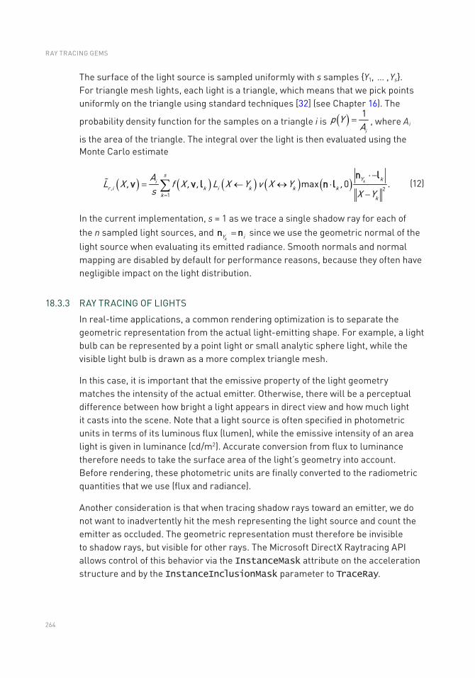
264
The surface of the light source is sampled uniformly with s samples Y1, … , Ys. For triangle mesh lights, each light is a triangle, which means that we pick points uniformly on the triangle using standard techniques [32] (see Chapter 16). The
probability density function for the samples on a triangle i is ( )i
p yA1
= , where Ai
is the area of the triangle. The integral over the light is then evaluated using the Monte Carlo estimate
( ) ( ) ( ) ( ) ( ) ks
y kir i k i k k k
k k
AX , f X , , L X y v X y ,
s XL
y, 2
1
max 0 .=
× -= ¬ « ×
-å
n lv v l n l (12)
In the current implementation, s = 1 as we trace a single shadow ray for each of the n sampled light sources, and
ky i=n n since we use the geometric normal of the light source when evaluating its emitted radiance. Smooth normals and normal mapping are disabled by default for performance reasons, because they often have negligible impact on the light distribution.
18.3.3 RAy TRACING OF LIGHTS
In real-time applications, a common rendering optimization is to separate the geometric representation from the actual light-emitting shape. For example, a light bulb can be represented by a point light or small analytic sphere light, while the visible light bulb is drawn as a more complex triangle mesh.
In this case, it is important that the emissive property of the light geometry matches the intensity of the actual emitter. Otherwise, there will be a perceptual difference between how bright a light appears in direct view and how much light it casts into the scene. Note that a light source is often specified in photometric units in terms of its luminous flux (lumen), while the emissive intensity of an area light is given in luminance (cd/m2). Accurate conversion from flux to luminance therefore needs to take the surface area of the light’s geometry into account. Before rendering, these photometric units are finally converted to the radiometric quantities that we use (flux and radiance).
Another consideration is that when tracing shadow rays toward an emitter, we do not want to inadvertently hit the mesh representing the light source and count the emitter as occluded. The geometric representation must therefore be invisible to shadow rays, but visible for other rays. The Microsoft DirectX Raytracing API allows control of this behavior via the InstanceMask attribute on the acceleration structure and by the InstanceInclusionMask parameter to TraceRay.
RAY TRACING GEMS
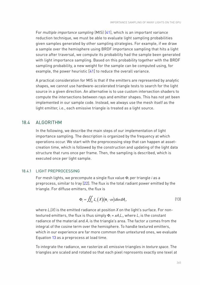
265
For multiple importance sampling (MIS) [41], which is an important variance reduction technique, we must be able to evaluate light sampling probabilities given samples generated by other sampling strategies. For example, if we draw a sample over the hemisphere using BRDF importance sampling that hits a light source after traversal, we compute its probability had the sample been generated with light importance sampling. Based on this probability together with the BRDF sampling probability, a new weight for the sample can be computed using, for example, the power heuristic [41] to reduce the overall variance.
A practical consideration for MIS is that if the emitters are represented by analytic shapes, we cannot use hardware-accelerated triangle tests to search for the light source in a given direction. An alternative is to use custom intersection shaders to compute the intersections between rays and emitter shapes. This has not yet been implemented in our sample code. Instead, we always use the mesh itself as the light emitter, i.e., each emissive triangle is treated as a light source.
18.4 ALGORITHM
In the following, we describe the main steps of our implementation of light importance sampling. The description is organized by the frequency at which operations occur. We start with the preprocessing step that can happen at asset-creation time, which is followed by the construction and updating of the light data structure that runs once per frame. Then, the sampling is described, which is executed once per light sample.
18.4.1 LIGHT PREPROCESSING
For mesh lights, we precompute a single flux value Φi per triangle i as a preprocess, similar to Iray [22]. The flux is the total radiant power emitted by the triangle. For diffuse emitters, the flux is
( )( )w wòòWF = ×i i i iL X d dA ,n (13)
where Li(X) is the emitted radiance at position X on the light’s surface. For non- textured emitters, the flux is thus simply Φi = πAiLi, where Li is the constant radiance of the material and Ai is the triangle’s area. The factor π comes from the integral of the cosine term over the hemisphere. To handle textured emitters, which in our experience are far more common than untextured ones, we evaluate Equation 13 as a preprocess at load time.
To integrate the radiance, we rasterize all emissive triangles in texture space. The triangles are scaled and rotated so that each pixel represents exactly one texel at
IMPORTANCE SAMPLING OF MANy LIGHTS ON THE GPU
266
the largest mip level. The integral is then computed by loading the radiance for the corresponding texel in the pixel shader and by accumulating its value atomically. We also count the number of texels and divide by that number at the end.
The only side effect of the pixel shader is atomic additions to a buffer of per-triangle values. Due to the current lack of floating-point atomics in DirectX 12, we use an NVIDIA extension via NVAPI [26] to do floating-point atomic addition.
Since the pixel shader has no render target bound (i.e., it is a void pixel shader), we can make the viewport arbitrarily large within the API limits, without worrying about memory consumption. The vertex shader loads the UV texture coordinates from memory and places the triangle at an appropriate coordinate in texture space so that it is always within the viewport. For example, if texture wrapping is enabled, the triangle is rasterized at pixel coordinates
( ) ( ) ( )x, y u u ,v v w,h ,= - ê ú - ê ú ×ë û ë û (14)
where w, h are the dimensions of the largest mip level of the emissive texture. With this transform, the triangle is always in view, independent of the magnitude of its (pre- wrapped) UV coordinates.
We currently rasterize the triangle using one sample per pixel, and hence only accumulate texels whose centers are covered. Tiny triangles that do not cover any texels are assigned a default nonzero flux to ensure convergence. Multisampling, or conservative rasterization with analytic coverage computations in the pixel shader, can be used to improve accuracy of the computed flux values.
All triangles with Φi = 0 are excluded from further processing. Culling of zero flux triangles is an important practical optimization. In several example scenes, the majority of the emissive triangles lie in black regions of the emissive textures. This is not surprising, as often the emissiveness is painted into larger textures, rather than splitting the mesh into emissive and non-emissive meshes with separate materials.
18.4.2 ACCELERATION STRUCTURE
We are using a similar acceleration structure as Conty Estevez and Kulla [11], that is, a bounding volume hierarchy [10, 33] built from top to bottom using binning [43]. Our implementation uses a binary BVH, meaning that each node has two children. In some cases, a wider branching factor may be beneficial.
We will briefly introduce how binning works, before presenting different existing heuristics used during the building process, as well as minor variants thereof.
RAY TRACING GEMS
267
18.4.2.1 BUILDING THE BVH
When building a binary BVH from top to bottom, the quality and speed at which the tree is built depends on how the triangles are split between the left and right children at each node. Analyzing all the potential split locations will yield the best results, but this will also be slow and is not suitable for real-time applications.
The approach taken by Wald [43] consists of uniformly partitioning the space at each node into bins and then running the split analysis on those bins only. This implies that the more bins one has, the higher the quality of the generated tree will be, but the tree will also be more costly to build.
18.4.2.2 LIGHT ORIENTATION CONE
To help take into account the orientation of the different light sources, Conty Estevez and Kulla [11] store a light orientation cone in each node. This cone is made of an axis and two angles, θo and θe: the former bounds the normals of all emitters found within the node, whereas the latter bounds the set of directions in which light gets emitted (around each normal).
For example, a single-sided emissive triangle would have θo = 0 (there is only
one normal) and q p=e 2
(it emits light over the whole hemisphere). Alternatively,
an emissive sphere would have θo = π (it has normals pointing in all directions)
and q p=e 2
, as around each normal, light is still only emitted over the whole
hemisphere; θe will often be p2
, except for lights with a directional emission profile
or for spotlights, where it will be equal to the spotlight’s cone angle.
When computing the cone for a parent node, its θo will be computed such that it encompasses all the normals found in its children, whereas θe is simply computed as the maximum of each child’s θe.
18.4.2.3 DEFINING THE SPLIT PLANE
As mentioned earlier, an axis-aligned split plane has to be computed to split the set of lights into two subsets, one for each child. This is usually achieved by computing a cost metric for each possible split and picking the one with the lowest cost. In the context of a binned BVH, we tested the surface area heuristic (SAH) (introduced by Goldsmith and Salmon [14] and formalized by MacDonald and Booth [24]) and the surface area orientation heuristic (SAOH) [11], as well as different variants of those two methods.
IMPORTANCE SAMPLING OF MANy LIGHTS ON THE GPU
268
For all the variants presented below, the binning performed while building the BVH can be done either on the largest axis only (of a node’s axis-aligned bounding box (AABB)) or on all three axes and the split with the lowest cost is selected. Only considering the largest axis will result in lower build time but also lower tree quality, especially for the variants taking the light orientations into account. More details on those trade-offs can be found in Section 18.5.
SAH The SAH focuses on the surface area of the AABB of the resulting children as well as on the number of lights that they contain. If we define the left child as
ij jL 0bin== È and the right child as k
j i jR 1bin= += È , where k is the number of bins and
i ∈ [0, k − 1], the cost for the split creating L and R as children is
( ) ( ) ( ) ( ) ( )( ) ( )
n L a L n R a Rcost L,R
n L R a L R,
+=
È È (15)
where n(C) and a(C) return the number of lights and the surface area of a potential child node C, respectively.
SAOH The SAOH is based on the SAH and includes two additional weights: one based on the bounding cone around the directions in which the lights emit light, and another based on the flux emitted by the resulting clusters. The cost metric is
( ) ( ) ( ) ( ) ( ) ( ) ( ) ( )( ) ( )r
L a L M L R a R M RL,R, s k s
a L R M L Rcost ,W W
W
F +F=
È È (16)
where s is the axis on which the split is occurring, kr(s) = lengthmax/lengths is used to prevent thin boxes, and MΩ is an orientation measure [11].
VH The volume heuristic (VH) is based on the SAH and replaces the surface area measure a(C) in Equation 15 by the volume v(C) of a node C’s AABB.
VOH The volume orientation heuristic (VOH) similarly replaces the surface area measure in the SAOH (Equation 16) by the volume measure.
18.4.3 LIGHT IMPORTANCE SAMPLING
We now look at how the lights are actually sampled based on the acceleration structure described in the previous section. First, the light BVH is probabilistically traversed in order to select a single light source, and then a light sample is generated on the surface of that light (if it is an area light). See Figure 18-1.
RAY TRACING GEMS
269
18.4.3.1 PROBABILISTIC BVH TRAVERSAL
When traversing the acceleration data structure, we want to select the node that will lead us to the lights that contribute the most to the current shading point, with a probability for each light that is proportional to its contribution. As mentioned in Section 18.4.2, the contribution depends on many parameters. We will use either approximations or the exact value for each parameter, and we will try different combinations to optimize quality versus performance.
Distance This parameter is computed as the distance between the shading point and the center of the AABB of the node being considered. This favors nodes that are close to the shading point (and by extension lights that are close), if the node has a small AABB. However, in the first levels of the BVH, the nodes have large AABBs that contain most of the scene, giving a poor approximation of the actual distance between the shading point and some of the lights contained within that node.
Light Flux The flux of a node is computed as the sum of the flux emitted by all light sources contained within that node. This is actually precomputed when building the BVH for performance reasons; if some light sources have changing flux values over time, the precomputation will not be an issue because the BVH will have to be rebuilt anyway since the flux is also used for guiding the building step.
Light Orientation The selection so far does not take into consideration the orientation of the light source, which could give as much weight to a light source that is shining directly upon the shading point as to another light source that is backfacing. To that end, Conty Estevez and Kulla [11] introduced an additional term to a node’s importance function that conservatively estimates the angle between the light normal and direction from the node’s AABB center to the shading point.
Light Visibility To avoid considering lights that are located below the horizon of a shading point, we use the clamped n ⋅ l term in the importance function of each node. Note that Conty Estevez and Kulla [11] use this clamped term, multiplied by the surface’s albedo, as an approximation to the diffuse BRDF, which will achieve the same effect of discarding lights that are beneath the horizon of the shading point.
Node Importance Using the different parameters just defined, the importance function given a shading point X and a child node C is defined as
( ) ( ) q q q qF ì <= ´
¢ ¢ ¢íî-
i eC
X ,CX C
2
cos cos if ,importance
0 otherwise,
∣ ∣ (17)
IMPORTANCE SAMPLING OF MANy LIGHTS ON THE GPU
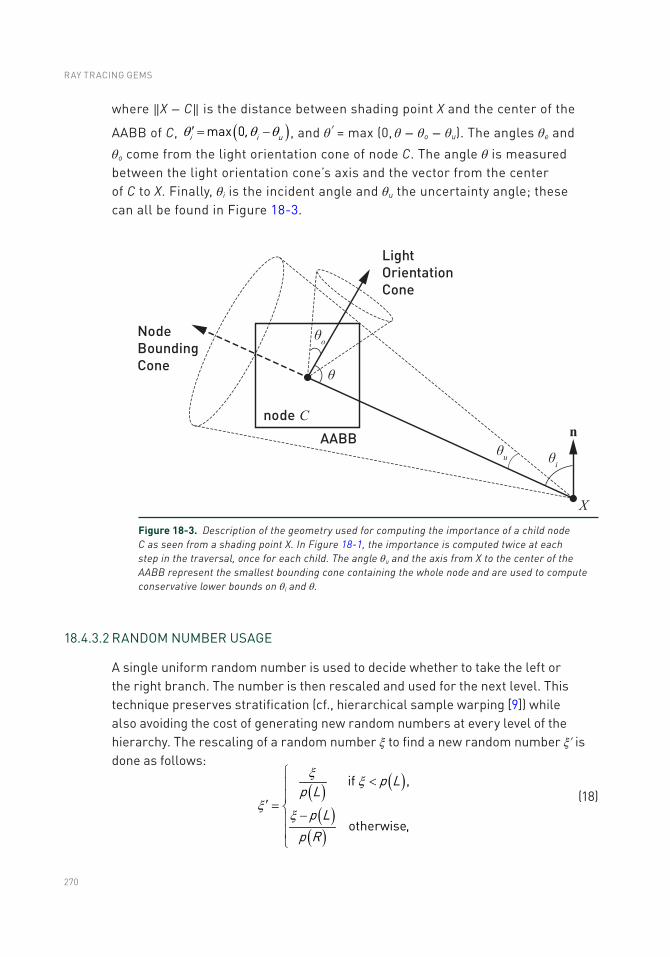
270
where ‖X − C‖ is the distance between shading point X and the center of the
AABB of C, ( )max 0i i u,q q q= -¢ , and θʹ = max (0, θ − θo − θu). The angles θe and
θo come from the light orientation cone of node C. The angle θ is measured between the light orientation cone’s axis and the vector from the center of C to X. Finally, θi is the incident angle and θu the uncertainty angle; these can all be found in Figure 18-3.
Figure 18-3. Description of the geometry used for computing the importance of a child node C as seen from a shading point X. In Figure 18-1, the importance is computed twice at each step in the traversal, once for each child. The angle θu and the axis from X to the center of the AABB represent the smallest bounding cone containing the whole node and are used to compute conservative lower bounds on θi and θ.
18.4.3.2 RANDOM NUMBER USAGE
A single uniform random number is used to decide whether to take the left or the right branch. The number is then rescaled and used for the next level. This technique preserves stratification (cf., hierarchical sample warping [9]) while also avoiding the cost of generating new random numbers at every level of the hierarchy. The rescaling of a random number ξ to find a new random number ξʹ is done as follows:
( ) ( )
( )( )
p Lp L
p Lp R
if ,
otherwise,
x
xx
xì<ï
ï= í¢-ï
ïî
(18)
RAY TRACING GEMS
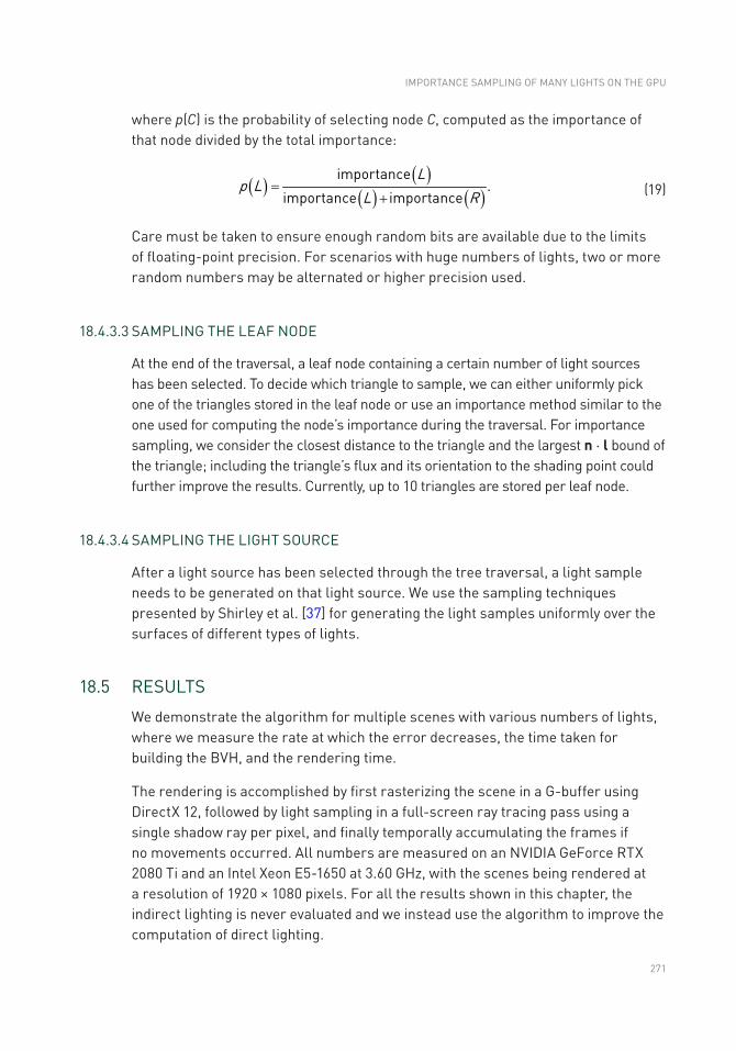
271
where p(C) is the probability of selecting node C, computed as the importance of that node divided by the total importance:
( ) ( )( ) ( )
Lp L
L Rimportance
.importance importance
=+ (19)
Care must be taken to ensure enough random bits are available due to the limits of floating-point precision. For scenarios with huge numbers of lights, two or more random numbers may be alternated or higher precision used.
18.4.3.3 SAMPLING THE LEAF NODE
At the end of the traversal, a leaf node containing a certain number of light sources has been selected. To decide which triangle to sample, we can either uniformly pick one of the triangles stored in the leaf node or use an importance method similar to the one used for computing the node’s importance during the traversal. For importance sampling, we consider the closest distance to the triangle and the largest n ⋅ l bound of the triangle; including the triangle’s flux and its orientation to the shading point could further improve the results. Currently, up to 10 triangles are stored per leaf node.
18.4.3.4 SAMPLING THE LIGHT SOURCE
After a light source has been selected through the tree traversal, a light sample needs to be generated on that light source. We use the sampling techniques presented by Shirley et al. [37] for generating the light samples uniformly over the surfaces of different types of lights.
18.5 RESULTS
We demonstrate the algorithm for multiple scenes with various numbers of lights, where we measure the rate at which the error decreases, the time taken for building the BVH, and the rendering time.
The rendering is accomplished by first rasterizing the scene in a G-buffer using DirectX 12, followed by light sampling in a full-screen ray tracing pass using a single shadow ray per pixel, and finally temporally accumulating the frames if no movements occurred. All numbers are measured on an NVIDIA GeForce RTX 2080 Ti and an Intel Xeon E5-1650 at 3.60 GHz, with the scenes being rendered at a resolution of 1920 × 1080 pixels. For all the results shown in this chapter, the indirect lighting is never evaluated and we instead use the algorithm to improve the computation of direct lighting.
IMPORTANCE SAMPLING OF MANy LIGHTS ON THE GPU
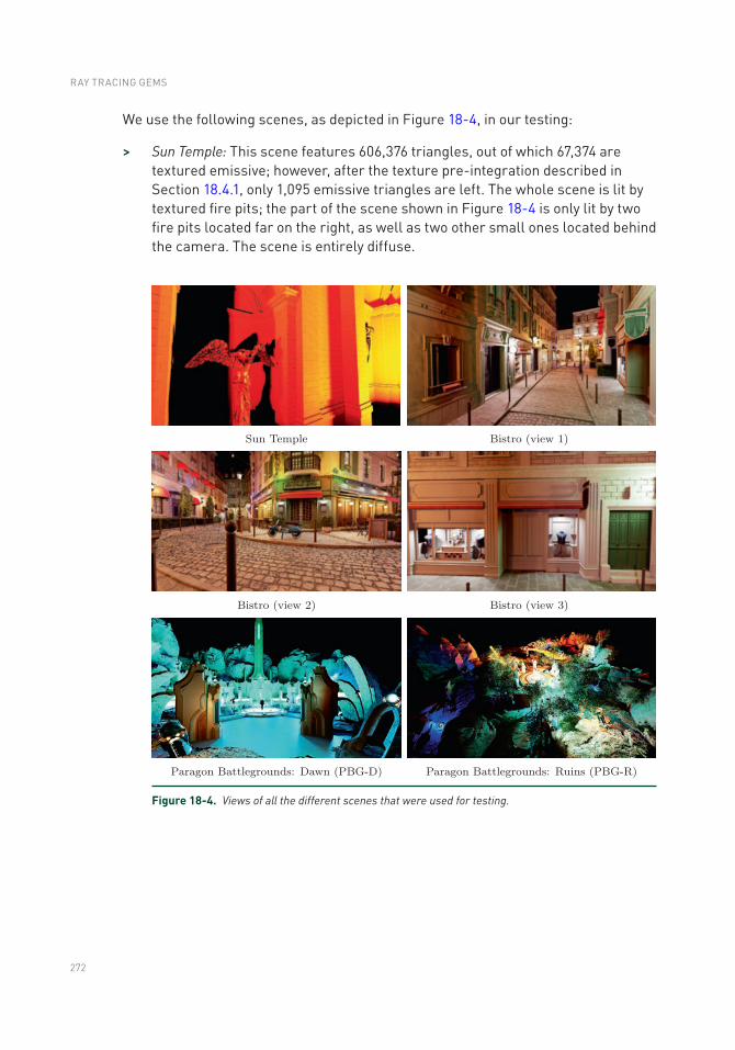
272
We use the following scenes, as depicted in Figure 18-4, in our testing:
> Sun Temple: This scene features 606,376 triangles, out of which 67,374 are textured emissive; however, after the texture pre-integration described in Section 18.4.1, only 1,095 emissive triangles are left. The whole scene is lit by textured fire pits; the part of the scene shown in Figure 18-4 is only lit by two fire pits located far on the right, as well as two other small ones located behind the camera. The scene is entirely diffuse.
Figure 18-4. Views of all the different scenes that were used for testing.
RAY TRACING GEMS
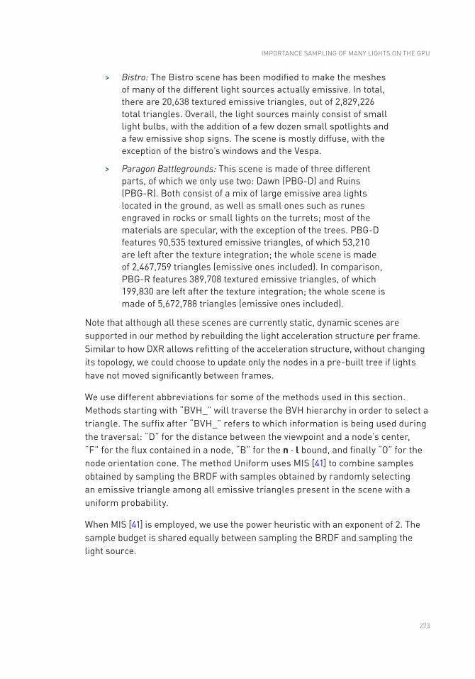
273
> Bistro: The Bistro scene has been modified to make the meshes of many of the different light sources actually emissive. In total, there are 20,638 textured emissive triangles, out of 2,829,226 total triangles. Overall, the light sources mainly consist of small light bulbs, with the addition of a few dozen small spotlights and a few emissive shop signs. The scene is mostly diffuse, with the exception of the bistro’s windows and the Vespa.
> Paragon Battlegrounds: This scene is made of three different parts, of which we only use two: Dawn (PBG-D) and Ruins (PBG-R). Both consist of a mix of large emissive area lights located in the ground, as well as small ones such as runes engraved in rocks or small lights on the turrets; most of the materials are specular, with the exception of the trees. PBG-D features 90,535 textured emissive triangles, of which 53,210 are left after the texture integration; the whole scene is made of 2,467,759 triangles (emissive ones included). In comparison, PBG-R features 389,708 textured emissive triangles, of which 199,830 are left after the texture integration; the whole scene is made of 5,672,788 triangles (emissive ones included).
Note that although all these scenes are currently static, dynamic scenes are supported in our method by rebuilding the light acceleration structure per frame. Similar to how DXR allows refitting of the acceleration structure, without changing its topology, we could choose to update only the nodes in a pre-built tree if lights have not moved significantly between frames.
We use different abbreviations for some of the methods used in this section. Methods starting with “BVH_” will traverse the BVH hierarchy in order to select a triangle. The suffix after “BVH_” refers to which information is being used during the traversal: “D” for the distance between the viewpoint and a node’s center, “F” for the flux contained in a node, “B” for the n ⋅ l bound, and finally “O” for the node orientation cone. The method Uniform uses MIS [41] to combine samples obtained by sampling the BRDF with samples obtained by randomly selecting an emissive triangle among all emissive triangles present in the scene with a uniform probability.
When MIS [41] is employed, we use the power heuristic with an exponent of 2. The sample budget is shared equally between sampling the BRDF and sampling the light source.
IMPORTANCE SAMPLING OF MANy LIGHTS ON THE GPU
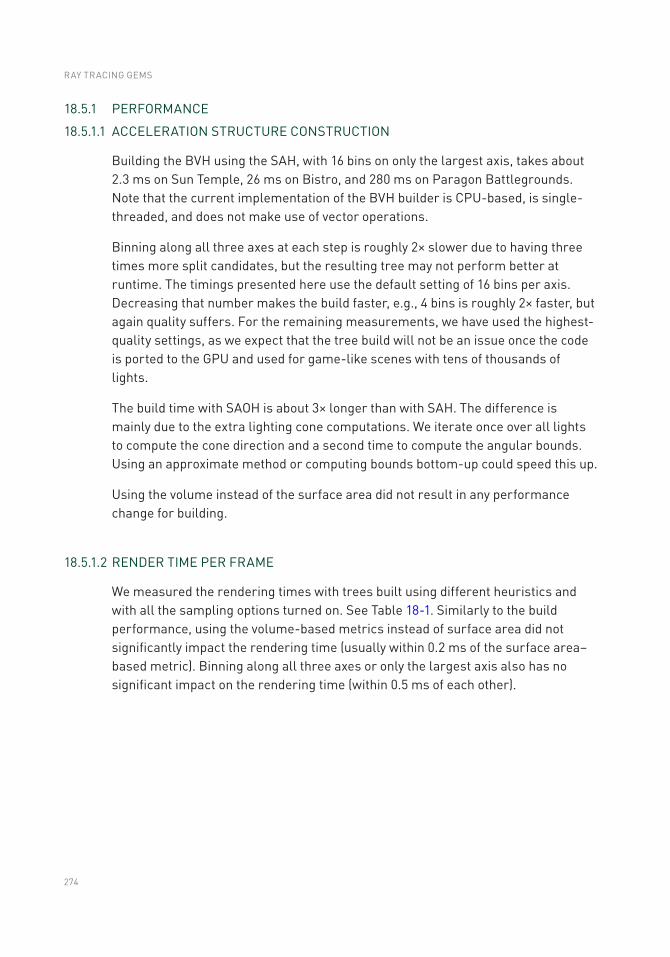
274
18.5.1 PERFORMANCE
18.5.1.1 ACCELERATION STRUCTURE CONSTRUCTION
Building the BVH using the SAH, with 16 bins on only the largest axis, takes about 2.3 ms on Sun Temple, 26 ms on Bistro, and 280 ms on Paragon Battlegrounds. Note that the current implementation of the BVH builder is CPU-based, is single-threaded, and does not make use of vector operations.
Binning along all three axes at each step is roughly 2× slower due to having three times more split candidates, but the resulting tree may not perform better at runtime. The timings presented here use the default setting of 16 bins per axis. Decreasing that number makes the build faster, e.g., 4 bins is roughly 2× faster, but again quality suffers. For the remaining measurements, we have used the highest-quality settings, as we expect that the tree build will not be an issue once the code is ported to the GPU and used for game-like scenes with tens of thousands of lights.
The build time with SAOH is about 3× longer than with SAH. The difference is mainly due to the extra lighting cone computations. We iterate once over all lights to compute the cone direction and a second time to compute the angular bounds. Using an approximate method or computing bounds bottom-up could speed this up.
Using the volume instead of the surface area did not result in any performance change for building.
18.5.1.2 RENDER TIME PER FRAME
We measured the rendering times with trees built using different heuristics and with all the sampling options turned on. See Table 18-1. Similarly to the build performance, using the volume-based metrics instead of surface area did not significantly impact the rendering time (usually within 0.2 ms of the surface area–based metric). Binning along all three axes or only the largest axis also has no significant impact on the rendering time (within 0.5 ms of each other).
RAY TRACING GEMS
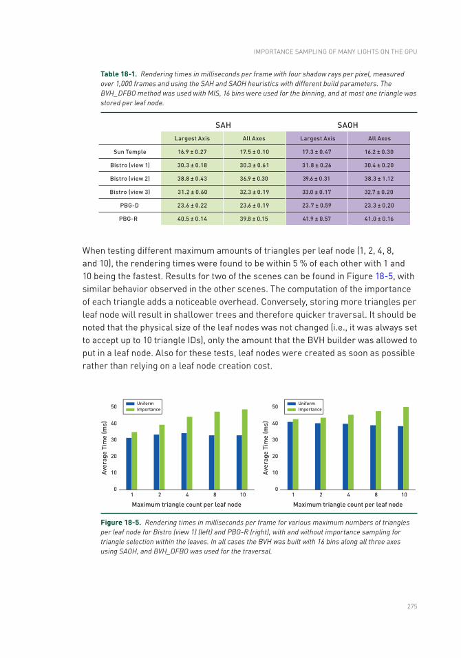
275
Table 18-1. Rendering times in milliseconds per frame with four shadow rays per pixel, measured over 1,000 frames and using the SAH and SAOH heuristics with different build parameters. The BVH_DFBO method was used with MIS, 16 bins were used for the binning, and at most one triangle was stored per leaf node.
When testing different maximum amounts of triangles per leaf node (1, 2, 4, 8, and 10), the rendering times were found to be within 5 % of each other with 1 and 10 being the fastest. Results for two of the scenes can be found in Figure 18-5, with similar behavior observed in the other scenes. The computation of the importance of each triangle adds a noticeable overhead. Conversely, storing more triangles per leaf node will result in shallower trees and therefore quicker traversal. It should be noted that the physical size of the leaf nodes was not changed (i.e., it was always set to accept up to 10 triangle IDs), only the amount that the BVH builder was allowed to put in a leaf node. Also for these tests, leaf nodes were created as soon as possible rather than relying on a leaf node creation cost.
1 2 4 8 100
Aver
age
Tim
e (m
s)
Maximum triangle count per leaf node
10
20
30
40
50UniformImportance
1 2 4 8 100
Aver
age
Tim
e (m
s)
Maximum triangle count per leaf node
10
20
30
40
50UniformImportance
Figure 18-5. Rendering times in milliseconds per frame for various maximum numbers of triangles per leaf node for Bistro (view 1) (left) and PBG-R (right), with and without importance sampling for triangle selection within the leaves. In all cases the BVH was built with 16 bins along all three axes using SAOH, and BVH_DFBO was used for the traversal.
IMPORTANCE SAMPLING OF MANy LIGHTS ON THE GPU
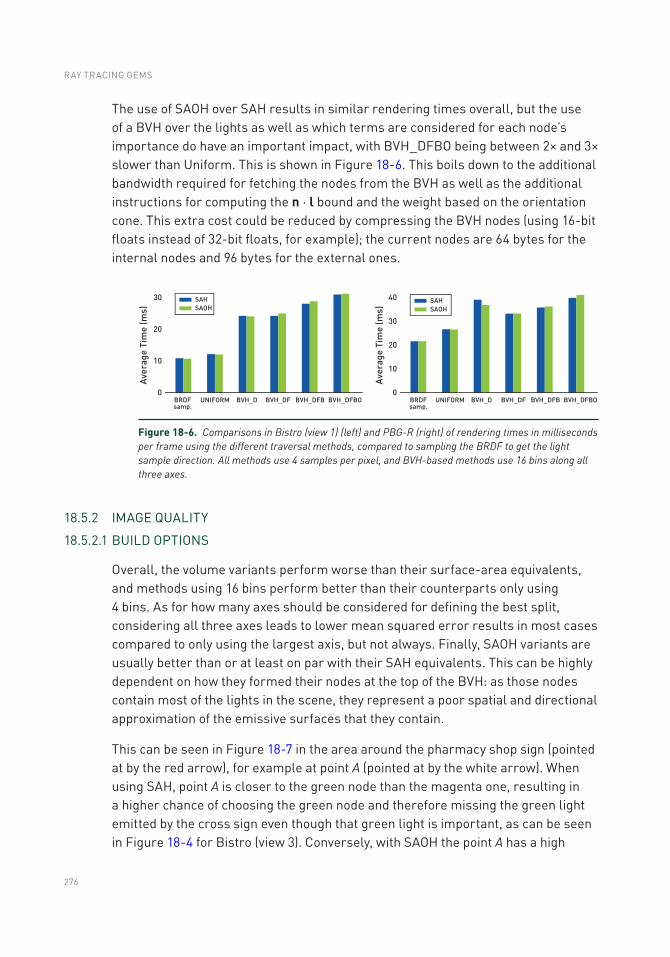
276
The use of SAOH over SAH results in similar rendering times overall, but the use of a BVH over the lights as well as which terms are considered for each node’s importance do have an important impact, with BVH_DFBO being between 2× and 3× slower than Uniform. This is shown in Figure 18-6. This boils down to the additional bandwidth required for fetching the nodes from the BVH as well as the additional instructions for computing the n ⋅ l bound and the weight based on the orientation cone. This extra cost could be reduced by compressing the BVH nodes (using 16-bit floats instead of 32-bit floats, for example); the current nodes are 64 bytes for the internal nodes and 96 bytes for the external ones.
BRDFsamp.
UNIFORM BVH_D BVH_DF BVH_DFB BVH_DFBO0
Aver
age
Tim
e (m
s)
10
20
30 SAHSAOH
BRDFsamp.
UNIFORM BVH_D BVH_DF BVH_DFB BVH_DFBO0
Aver
age
Tim
e (m
s)10
20
40
30
SAHSAOH
Figure 18-6. Comparisons in Bistro (view 1) (left) and PBG-R (right) of rendering times in milliseconds per frame using the different traversal methods, compared to sampling the BRDF to get the light sample direction. All methods use 4 samples per pixel, and BVH-based methods use 16 bins along all three axes.
18.5.2 IMAGE QUALITy
18.5.2.1 BUILD OPTIONS
Overall, the volume variants perform worse than their surface-area equivalents, and methods using 16 bins perform better than their counterparts only using 4 bins. As for how many axes should be considered for defining the best split, considering all three axes leads to lower mean squared error results in most cases compared to only using the largest axis, but not always. Finally, SAOH variants are usually better than or at least on par with their SAH equivalents. This can be highly dependent on how they formed their nodes at the top of the BVH: as those nodes contain most of the lights in the scene, they represent a poor spatial and directional approximation of the emissive surfaces that they contain.
This can be seen in Figure 18-7 in the area around the pharmacy shop sign (pointed at by the red arrow), for example at point A (pointed at by the white arrow). When using SAH, point A is closer to the green node than the magenta one, resulting in a higher chance of choosing the green node and therefore missing the green light emitted by the cross sign even though that green light is important, as can be seen in Figure 18-4 for Bistro (view 3). Conversely, with SAOH the point A has a high
RAY TRACING GEMS
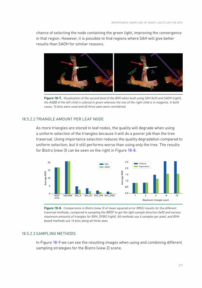
277
chance of selecting the node containing the green light, improving the convergence in that region. However, it is possible to find regions where SAH will give better results than SAOH for similar reasons.
18.5.2.2 TRIANGLE AMOUNT PER LEAF NODE
As more triangles are stored in leaf nodes, the quality will degrade when using a uniform selection of the triangles because it will do a poorer job than the tree traversal. Using importance selection reduces the quality degradation compared to uniform selection, but it still performs worse than using only the tree. The results for Bistro (view 3) can be seen on the right in Figure 18-8.
Figure 18-7. Visualization of the second level of the BVH when built using SAH (left) and SAOH (right); the AABB of the left child is colored in green whereas the one of the right child is in magenta. In both cases, 16 bins were used and all three axes were considered.
BRDFsamp.
UNIFORM BVH_D BVH_DF BVH_DFB BVH_DFBO
Aver
age
MSE
0
5
10
15
20SAHSAOH
1 2 4 8 10
Aver
age
MSE
Maximum triangle count
0.0
0/5
1.0
1.5
2.5
2.0
UniformImportance
Figure 18-8. Comparisons in Bistro (view 3) of mean squared error (MSE) results for the different traversal methods, compared to sampling the BRDF to get the light sample direction (left) and various maximum amounts of triangles for BVH_DFBO (right). All methods use 4 samples per pixel, and BVH-based methods use 16 bins along all three axes.
18.5.2.3 SAMPLING METHODS
In Figure 18-9 we can see the resulting images when using and combining different sampling strategies for the Bistro (view 2) scene.
IMPORTANCE SAMPLING OF MANy LIGHTS ON THE GPU
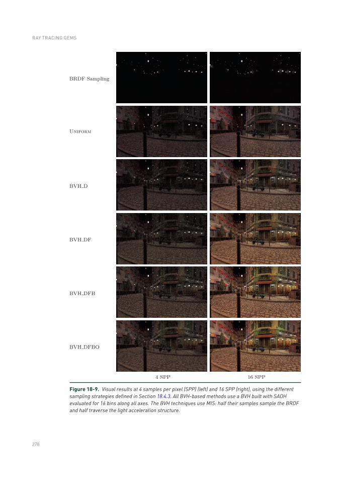
278
Figure 18-9. Visual results at 4 samples per pixel (SPP) (left) and 16 SPP (right), using the different sampling strategies defined in Section 18.4.3. All BVH-based methods use a BVH built with SAOH evaluated for 16 bins along all axes. The BVH techniques use MIS: half their samples sample the BRDF and half traverse the light acceleration structure.
RAY TRACING GEMS
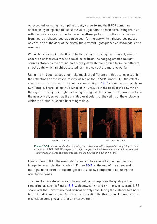
279
As expected, using light sampling greatly outperforms the BRDF sampling approach, by being able to find some valid light paths at each pixel. Using the BVH with the distance as an importance value allows picking up of the contributions from nearby light sources, as can be seen for the two white light sources placed on each side of the door of the bistro, the different lights placed on its facade, or its windows.
When also considering the flux of the light sources during the traversal, we can observe a shift from a mostly blueish color (from the hanging small blue light sources closest to the ground) to a more yellowish tone coming from the different street lights, which might be located farther away but are more powerful.
Using the n ⋅ l bounds does not make much of a difference in this scene, except for the reflections on the Vespa (mostly visible on the 16 SPP images), but the effects can be way more pronounced in other scenes. Figure 18-10 shows an example from Sun Temple. There, using the bounds on n ⋅ l results in the back of the column on the right receiving more light and being distinguishable from the shadow it casts on the nearby wall, as well as the architectural details of the ceiling of the enclave in which the statue is located becoming visible.
Figure 18-10. Visual results when not using the n ⋅ l bounds (left) compared to using it (right). Both images use 8 SPP (4 BRDF samples and 4 light samples) and a BVH binned along all three axes with 16 bins using SAH, and both take into account the distance and flux of the light.
Even without SAOH, the orientation cone still has a small impact on the final image; for example, the facades in Figure 18-9 (at the end of the street and in the right-hand corner of the image) are less noisy compared to not using the orientation cones.
The use of an acceleration structure significantly improves the quality of the rendering, as seen in Figure 18-8, with between 4× and 6× improved average MSE score over the Uniform method even when only considering the distance to a node for that node’s importance function. Incorporating the flux, the n ⋅ l bound and the orientation cone give a further 2× improvement.
IMPORTANCE SAMPLING OF MANy LIGHTS ON THE GPU
280
18.6 CONCLUSION
We have presented a hierarchical data structure and sampling methods to accelerate light importance sampling in real-time ray tracing, similar to what is used in offline rendering [11, 22]. We have explored sampling performance on the GPU, taking advantage of hardware-accelerated ray tracing. We have also presented results using different build heuristics. We hope this work will inspire future work in game engines and research to incorporate better sampling strategies.
While the focus of this chapter has been on the sampling problem, it should be noted that any sample-based method usually needs to be paired with some form of denoising filter to remove the residual noise, and we refer the reader to recent real-time methods based on advanced bilateral kernels [25, 34, 35] as a suitable place to start. Deep learning–based methods [3, 7, 42] also show great promise. For an overview of traditional techniques, refer to the survey by Zwicker et al. [48].
For the sampling, there are a number of worthwhile avenues for improvement. In the current implementation, we bound n ⋅ l to cull lights under the horizon. It would be helpful to also incorporate BRDF and visibility information to refine the sampling probabilities during tree traversal. On the practical side, we want to move the BVH building code to the GPU for performance reasons. That will also be important for supporting lights on dynamic or skinned geometry.
ACKNOWLEDGEMENTS
Thanks to Nicholas Hull and Kate Anderson for creating the test scenes. The Sun Temple [13] and Paragon Battlegrounds scenes are based on assets kindly donated by Epic Games. The Bistro scene is based on assets kindly donated by Amazon Lumberyard [1]. Thanks to Benty et al. [4] for creating the Falcor rendering research framework, and to He et al. [16] and Jonathan Small for the Slang shader compiler that Falcor uses. We would also like to thank Pierre Moreau’s advisor Michael Doggett at Lund University. Lastly, thanks to Aaron Lefohn and NVIDIA Research for supporting this work.
REFERENCES
[1] Amazon Lumberyard. Amazon Lumberyard Bistro, Open Research Content Archive (ORCA). http://developer.nvidia.com/orca/amazon-lumberyard-bistro, July 2017.
[2] Andersson, J. Parallel Graphics in Frostbite—Current & Future. Beyond Programmable Shading, SIGGRAPH Courses, 2009.
RAY TRACING GEMS
281
[3] Bako, S., Vogels, T., McWilliams, B., Meyer, M., Novák, J., Harvill, A., Sen, P., DeRose, T., and Rousselle, F. Kernel-Predicting Convolutional Networks for Denoising Monte Carlo Renderings. ACM Transactions on Graphics 36, 4 (2017), 97:1–97:14.
[4] Benty, N., yao, K.-H., Foley, T., Kaplanyan, A. S., Lavelle, C., Wyman, C., and Vijay, A. The Falcor Rendering Framework. https://github.com/NVIDIAGameWorks/Falcor, July 2017.
[5] Bikker, J. Real-Time Ray Tracing Through the Eyes of a Game Developer. In IEEE Symposium on Interactive Ray Tracing (2007), pp. 1–10.
[6] Bikker, J. Ray Tracing in Real-Time Games. PhD thesis, Delft University, 2012.
[7] Chaitanya, C. R. A., Kaplanyan, A. S., Schied, C., Salvi, M., Lefohn, A., Nowrouzezahrai, D., and Aila, T. Interactive Reconstruction of Monte Carlo Image Sequences Using a Recurrent Denoising Autoencoder. ACM Transactions on Graphics 36, 4 (2017), 98:1–98:12.
[8] Christensen, P. H., and Jarosz, W. The Path to Path-Traced Movies. Foundations and Trends in Computer Graphics and Vision 10, 2 (2016), 103–175.
[9] Clarberg, P., Jarosz, W., Akenine-Möller, T., and Jensen, H. W. Wavelet Importance Sampling: Efficiently Evaluating Products of Complex Functions. ACM Transactions on Graphics 24, 3 (2005), 1166–1175.
[10] Clark, J. H. Hierarchical Geometric Models for Visibility Surface Algorithms. Communications of the ACM 19, 10 (1976), 547–554.
[11] Conty Estevez, A., and Kulla, C. Importance Sampling of Many Lights with Adaptive Tree Splitting. Proceedings of the ACM on Computer Graphics and Interactive Techniques 1, 2 (2018), 25:1–25:17.
[12] Dachsbacher, C., Křivánek, J., Hašan, M., Arbree, A., Walter, B., and Novák, J. Scalable Realistic Rendering with Many-Light Methods. Computer Graphics Forum 33, 1 (2014), 88–104.
[13] Epic Games. Unreal Engine Sun Temple, Open Research Content Archive (ORCA). http://developer.nvidia.com/orca/epic-games-sun-temple, October 2017.
[14] Goldsmith, J., and Salmon, J. Automatic Creation of Object Hierarchies for Ray Tracing. IEEE Computer Graphics and Applications 7, 5 (1987), 14–20.
[15] Harada, T. A 2.5D Culling for Forward+. In SIGGRAPH Asia 2012 Technical Briefs (2012), pp. 18:1–18:4.
[16] He, y., Fatahalian, K., and Foley, T. Slang: Language Mechanisms for Extensible Real-Time Shading Systems. ACM Transactions on Graphics 37, 4 (2018), 141:1–141:13.
[17] Heitz, E., Dupuy, J., Hill, S., and Neubelt, D. Real-Time Polygonal-Light Shading with Linearly Transformed Cosines. ACM Transactions on Graphics 35, 4 (2016), 41:1–41:8.
[18] Kajiya, J. T. The Rendering Equation. Computer Graphics (SIGGRAPH) (1986), 143–150.
[19] Karis, B. Real Shading in Unreal Engine 4. Physically Based Shading in Theory and Practice, SIGGRAPH Courses, August 2013.
[20] Keller, A. Instant Radiosity. In Proceedings of SIGGRAPH (1997), pp. 49–56.
[21] Keller, A., Fascione, L., Fajardo, M., Georgiev, I., Christensen, P., Hanika, J., Eisenacher, C., and Nichols, G. The Path Tracing Revolution in the Movie Industry. In ACM SIGGRAPH Courses (2015), pp. 24:1–24:7.
IMPORTANCE SAMPLING OF MANy LIGHTS ON THE GPU
282
[22] Keller, A., Wächter, C., Raab, M., Seibert, D., van Antwerpen, D., Korndörfer, J., and Kettner, L. The Iray Light Transport Simulation and Rendering System. arXiv, https://arxiv.org/abs/1705.01263, 2017.
[23] Lagarde, S., and de Rousiers, C. Moving Frostbite to Physically Based Rendering 3.0. Physically Based Shading in Theory and Practice, SIGGRAPH Courses, 2014.
[24] MacDonald, J. D., and Booth, K. S. Heuristics for Ray Tracing Using Space Subdivision. The Visual Computer 6, 3 (1990), 153–166.
[25] Mara, M., McGuire, M., Bitterli, B., and Jarosz, W. An Efficient Denoising Algorithm for Global Illumination. In Proceedings of High-Performance Graphics (2017), pp. 3:1–3:7.
[26] NVIDIA. NVAPI, 2018. https://developer.nvidia.com/nvapi.
[27] O’Donnell, y., and Chajdas, M. G. Tiled Light Trees. In Symposium on Interactive 3D Graphics and Games (2017), pp. 1:1–1:7.
[28] Olsson, O., and Assarsson, U. Tiled Shading. Journal of Graphics, GPU, and Game Tools 15, 4 (2011), 235–251.
[29] Olsson, O., Billeter, M., and Assarsson, U. Clustered Deferred and Forward Shading. In Proceedings of High-Performance Graphics (2012), pp. 87–96.
[30] Persson, E., and Olsson, O. Practical Clustered Deferred and Forward Shading. Advances in Real-Time Rendering in Games, SIGGRAPH Courses, 2013.
[31] Pharr, M. Guest Editor’s Introduction: Special Issue on Production Rendering. ACM Transactions on Graphics 37, 3 (2018), 28:1–28:4.
[32] Pharr, M., Jakob, W., and Humphreys, G. Physically Based Rendering: From Theory to Implementation, third ed. Morgan Kaufmann, 2016.
[33] Rubin, S. M., and Whitted, T. A 3-Dimensional Representation for Fast Rendering of Complex Scenes. Computer Graphics (SIGGRAPH) 14, 3 (1980), 110–116.
[34] Schied, C., Kaplanyan, A., Wyman, C., Patney, A., Chaitanya, C. R. A., Burgess, J., Liu, S., Dachsbacher, C., Lefohn, A., and Salvi, M. Spatiotemporal Variance- Guided Filtering: Real-Time Reconstruction for Path-Traced Global Illumination. In Proceedings of High-Performance Graphics (2017), pp. 2:1–2:12.
[35] Schied, C., Peters, C., and Dachsbacher, C. Gradient Estimation for Real-Time Adaptive Temporal Filtering. Proceedings of the ACM on Computer Graphics and Interactive Techniques 1, 2 (2018), 24:1–24:16.
[36] Schmittler, J., Pohl, D., Dahmen, T., Vogelgesang, C., and Slusallek, P. Realtime Ray Tracing for Current and Future Games. In ACM SIGGRAPH Courses (2005), pp. 23:1–23:5.
[37] Shirley, P., Wang, C., and Zimmerman, K. Monte Carlo Techniques for Direct Lighting Calculations. ACM Transactions on Graphics 15, 1 (1996), 1–36.
[38] Sobol, I. M. A Primer for the Monte Carlo Method. CRC Press, 1994.
[39] Talbot, J. F., Cline, D., and Egbert, P. Importance Resampling for Global Illumination. In Rendering Techniques (2005), pp. 139–146.
RAY TRACING GEMS
283
[40] Tokuyoshi, y., and Harada, T. Stochastic Light Culling. Journal of Computer Graphics Techniques 5, 1 (2016), 35–60.
[41] Veach, E., and Guibas, L. J. Optimally Combining Sampling Techniques for Monte Carlo Rendering. In Proceedings of SIGGRAPH (1995), pp. 419–428.
[42] Vogels, T., Rousselle, F., McWilliams, B., Röthlin, G., Harvill, A., Adler, D., Meyer, M., and Novák, J. Denoising with Kernel Prediction and Asymmetric Loss Functions. ACM Transactions on Graphics 37, 4 (2018), 124:1–124:15.
[43] Wald, I. On Fast Construction of SAH-Based Bounding Volume Hierarchies. In IEEE Symposium on Interactive Ray Tracing (2007), pp. 33–40.
[44] Walter, B., Arbree, A., Bala, K., and Greenberg, D. P. Multidimensional Lightcuts. ACM Transactions on Graphics 25, 3 (2006), 1081–1088.
[45] Walter, B., Fernandez, S., Arbree, A., Bala, K., Donikian, M., and Greenberg, D. P. Lightcuts: A Scalable Approach to Illumination. ACM Transactions on Graphics 24, 3 (2005), 1098–1107.
[46] Ward, G. J. Adaptive Shadow Testing for Ray Tracing. In Eurographics Workshop on Rendering (1991), pp. 11–20.
[47] Zimmerman, K., and Shirley, P. A Two-Pass Solution to the Rendering Equation with a Source Visibility Preprocess. In Rendering Techniques (1995), pp. 284–295.
[48] Zwicker, M., Jarosz, W., Lehtinen, J., Moon, B., Ramamoorthi, R., Rousselle, F., Sen, P., Soler, C., and yoon, S.-E. Recent Advances in Adaptive Sampling and Reconstruction for Monte Carlo Rendering. Computer Graphics Forum 34, 2 (2015), 667–681.
Open Access This chapter is licensed under the terms of the Creative Commons Attribution-NonCommercial-NoDerivatives 4.0 International License (http://creativecommons.org/licenses/by-nc-nd/4.0/), which permits any noncommercial use, sharing, distribution and
reproduction in any medium or format, as long as you give appropriate credit to the original author(s) and the source, provide a link to the Creative Commons license and indicate if you modified the licensed material. you do not have permission under this license to share adapted material derived from this chapter or parts of it.
The images or other third party material in this chapter are included in the chapter's Creative Commons license, unless indicated otherwise in a credit line to the material. If material is not included in the chapter's Creative Commons license and your intended use is not permitted by statutory regulation or exceeds the permitted use, you will need to obtain permission directly from the copyright holder.
IMPORTANCE SAMPLING OF MANy LIGHTS ON THE GPU
PART V
DENOISING AND FILTERING
287
PART V
Denoising and Filtering
Denoising and filtering are integral parts of a ray tracing pipeline. In a real-time setting, one can afford only a handful of rays per pixel, often randomly distributed. Consequently, the result is inherently noisy. By combining these sparse (but correct) per-pixel evaluations with spatiotemporal filters, variance is drastically reduced at the cost of increased bias, which is often a reasonable trade-off in real-time rendering. Furthermore, each ray is a point sample, which can introduce aliasing. By prefiltering terms where possible, e.g., texture lookups, aliasing can be reduced. This part introduces several practical examples of denoising and filtering for real-time ray tracing.
Chapter 19, “Cinematic Rendering in UE4 with Real-Time Ray Tracing and Denoising,” presents a detailed overview of integrating ray tracing in a modern game engine. By combining rasterization with GPU-accelerated DirectX Raytracing and custom denoising filters, the authors reach previously unseen image fidelity at interactive rates. In two comprehensive demos they showcase soft shadows, glossy reflections, and diffuse indirect illumination.
In rasterization-based rendering, one commonly applies texture filtering based on derivatives with respect to screen-space coordinates to reduce aliasing. This requires that primary visibility and shading are computed over quads of pixels. In ray tracing, explicit ray differentials are commonly used. In Chapter 20, “Texture Level of Detail Strategies for Real-Time Ray Tracing,” the authors evaluate techniques for texture filtering in a ray tracing setting and present several practical algorithms with different performance-versus-quality characteristics. In Chapter 21, “Simple Environment Map Filtering Using Ray Cones and Ray Differentials,” an inexpensive texture filtering technique for environment map lookups is presented.
Temporal antialiasing (TAA) reduces aliasing by reprojecting older samples using motion vectors and integrating samples over time. However, these techniques sometimes fail, e.g., in disocclusion regions. In Chapter 22, “Improving Temporal Antialiasing with Adaptive Ray Tracing,” the authors take advantage of adaptive ray tracing of primary visibility to reduce aliasing artifacts. Additional primary rays are traced in regions with high aliasing and in regions where TAA may fail. The approach is implemented with DirectX Raytracing in a modern game engine and approaches quality levels close to 16× supersampling.

288
Denoising and filtering are important building blocks for high-fidelity real-time rendering, and the chapters include many practical insights and readily applicable source code. In summary, this part shows that the combination of GPU-accelerated ray tracing and clever denoising techniques can produce convincing imagery at interactive rates.
Jacob Munkberg
289© NVIDIA 2019 E. Haines, T. Akenine-Möller (eds.), Ray Tracing Gems, https://doi.org/10.1007/978-1-4842-4427-2_19
CHAPTER 19
Cinematic Rendering in UE4 with Real-Time Ray Tracing and DenoisingEdward Liu,1 Ignacio Llamas,1 Juan Cañada,2 and Patrick Kelly2
1NVIDIA 2Epic Games
ABSTRACT
We present cinematic quality real-time rendering by integrating ray tracing in Unreal Engine 4. We improve the state-of-the-art performance in GPU ray tracing by an order of magnitude through a combination of engineering work, new ray tracing hardware, hybrid rendering techniques, and novel denoising algorithms.
19.1 INTRODUCTION
Image generation with ray tracing can produce higher-quality images than rasterization. One manifestation of this is that, in recent years, most special effects in films are done with path tracing. However, it is challenging to use ray tracing in real-time applications, e.g., games. Many steps of the ray tracing algorithm are costly, including bounding volume hierarchy (BVH) construction, BVH traversal, and ray/primitive intersection tests. Furthermore, stochastic sampling, which is commonly applied in ray tracing techniques, often requires hundreds to thousands of samples per pixel to produce a converged image. This is far outside the compute budget of modern real-time rendering techniques by several orders of magnitude. Also, until recently, real-time graphics APIs did not have ray tracing support, which made ray tracing integration in current games challenging. This changed in 2018 with the announcement of ray tracing support in DirectX 12 and Vulkan.
In this chapter we address many of these problems and demonstrate ray tracing integrated in a modern game engine: Unreal Engine 4 (UE4). Specifically:
> We adopted DirectX Raytracing (DXR) and integrated it into UE4, which allowed us to mostly reuse existing material shader code.
> We leveraged the RT Cores in the NVIDIA Turing architecture for hardware-accelerated BVH traversal and ray/triangle intersection tests.

290
> We invented novel reconstruction filters for high-quality stochastic rendering effects, including soft shadows, glossy reflections, diffuse global illumination, ambient occlusion, and translucency, with as few as one input sample per pixel.
A combination of hardware acceleration and software innovations enabled us to create two real-time cinematic-quality ray tracing–based demos: “Reflections” (Lucasfilm) and “Speed of Light” (Porsche).
19.2 INTEGRATING RAY TRACING IN UNREAL ENGINE 4
Integrating a ray tracing framework in a large application such as Unreal Engine is a challenging task, effectively one of the largest architectural changes since UE4 was released. Our goals while integrating ray tracing into UE4 were the following:
> Performance: This is a key aspect of UE4, so the ray tracing functionality should be aligned with what users expect. One of our decisions that helped performance is that the G-buffer is computed using existing rasterization-based techniques. On top of that, rays are traced to calculate specific passes, such as reflections or area light shadows.
> Compatibility: The output of the ray traced passes must be compatible with the existing UE4’s shading and post-processing pipeline.
> Shading consistency: Shading models used by UE4 must be accurately implemented with ray tracing to produce consistent shading results with existing shadings in UE4. Specifically, we strictly follow the same mathematics in existing shader code to do BRDF evaluation, importance sampling, and BRDF probability distribution function evaluation for various shading models provided by UE4.
> Minimizing disruption: Existing UE4 users should find the integration easy to understand and extend. As such, it must follow the UE design paradigms.
> Multiplatform support: While initially real-time ray tracing in UE4 is entirely based on DXR, the multiplatform nature of UE4 required us to design the new system in a way that makes it possible to eventually port it to other future solutions without a major refactoring.
The integration was split in two phases. The first was a prototyping phase, where we created the “Reflections” (a Lucasfilm Star Wars short movie made in collaboration with ILMxLabs) and “Speed of Light” (Porsche) demos with the goal of learning the ideal way of integrating the ray tracing technology within UE in a way that could scale properly in the future. That helped us extract conclusions on
RAY TRACING GEMS

291
the most challenging aspects of the integration: performance, API, integration in the deferred shading pipeline, changes required in the render hardware interface (RHI), a thin layer that abstracts the user from the specifics of each hardware platform, changes in the shader API, scalability, etc.
After finding answers to most of the questions that arose during phase one, we moved to phase two. This consisted of a major rewrite of the UE4 high-level rendering system, which in addition to providing a better integration of real-time ray tracing, also brought other advantages, including a significant overall performance boost.
19.2.1 PHASE 1: EXPERIMENTAL INTEGRATION
At a high level, integrating ray tracing into a rasterization-based real-time rendering engine consists of a few steps:
> Registering the geometry that will be ray traced, such that acceleration structures can be built or updated when changing.
> Creating hit shaders such that any time a ray hits a piece of geometry, we can compute its material parameters, just like we would have done in rasterization-based rendering.
> Creating ray generation shaders that trace rays for various use cases, such as shadows or reflections.
19.2.1.1 DIRECTX RAYTRACING BACKGROUND ON ACCELERATION STRUCTURES
To comprehend the first step, it is first useful to understand the two-level acceleration structure (AS) exposed by the DirectX Raytracing API. In DXR there are two types of acceleration structures, forming a two-level hierarchy: top-level acceleration structure (TLAS) and bottom-level acceleration structure (BLAS). These are illustrated in Figure 19-1. The TLAS is built over a set of instances, each one with its own transform matrix and a pointer to a BLAS. Each BLAS is built over a set of geometric primitives, either triangles or AABBs, where AABBs are used to enclose custom geometry that will be intersected using a custom Intersection shader executed during acceleration structure traversal as AABBs are found along a ray. The TLAS is usually rebuilt each frame for dynamic scenes. Each BLAS is built at least once for each unique piece of geometry. If the geometry is static, no additional BLAS build operations are needed after the initial build. For dynamic geometry, a BLAS will need to be either updated or fully rebuilt. A full BLAS rebuild is needed when the number of input primitives changes (i.e., when triangles or AABBs need to be added or removed, for example, due to dynamic tessellation or
CINEMATIC RENDERING IN UE4 WITH REAL-TIME RAY TRACING AND DENOISING
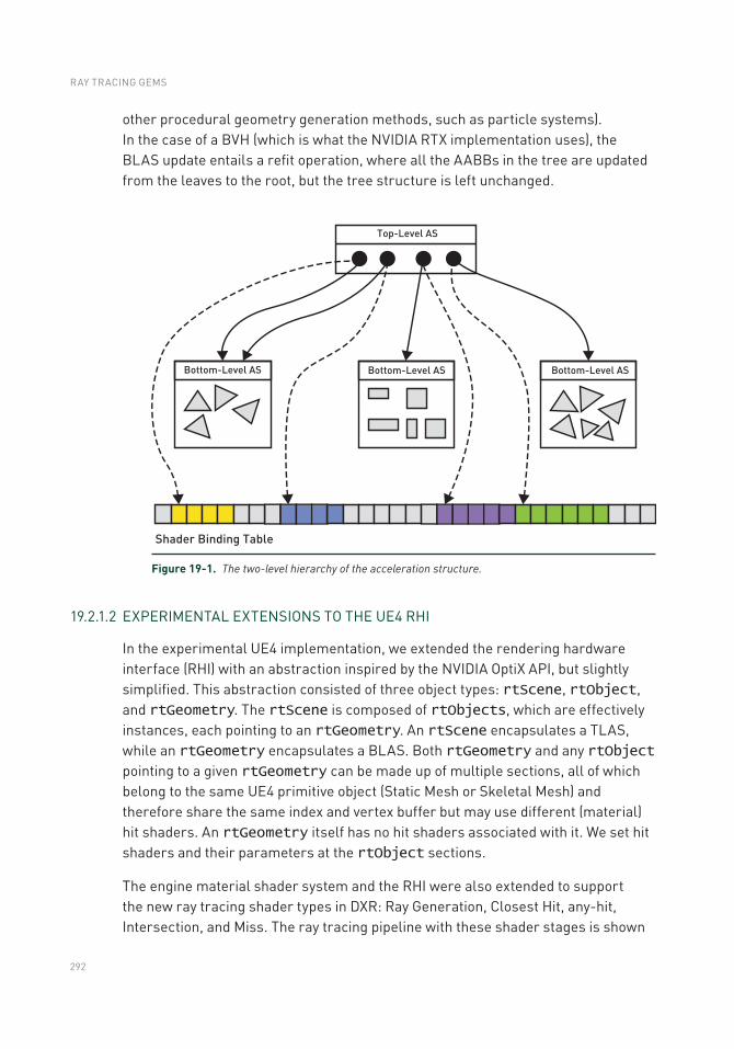
292
19.2.1.2 EXPERIMENTAL EXTENSIONS TO THE UE4 RHI
In the experimental UE4 implementation, we extended the rendering hardware interface (RHI) with an abstraction inspired by the NVIDIA OptiX API, but slightly simplified. This abstraction consisted of three object types: rtScene, rtObject, and rtGeometry. The rtScene is composed of rtObjects, which are effectively instances, each pointing to an rtGeometry. An rtScene encapsulates a TLAS, while an rtGeometry encapsulates a BLAS. Both rtGeometry and any rtObject pointing to a given rtGeometry can be made up of multiple sections, all of which belong to the same UE4 primitive object (Static Mesh or Skeletal Mesh) and therefore share the same index and vertex buffer but may use different (material) hit shaders. An rtGeometry itself has no hit shaders associated with it. We set hit shaders and their parameters at the rtObject sections.
The engine material shader system and the RHI were also extended to support the new ray tracing shader types in DXR: Ray Generation, Closest Hit, any-hit, Intersection, and Miss. The ray tracing pipeline with these shader stages is shown
other procedural geometry generation methods, such as particle systems). In the case of a BVH (which is what the NVIDIA RTX implementation uses), the BLAS update entails a refit operation, where all the AABBs in the tree are updated from the leaves to the root, but the tree structure is left unchanged.
Shader Binding Table
Top-Level AS
Bottom-Level AS Bottom-Level ASBottom-Level AS
Figure 19-1. The two-level hierarchy of the acceleration structure.
RAY TRACING GEMS
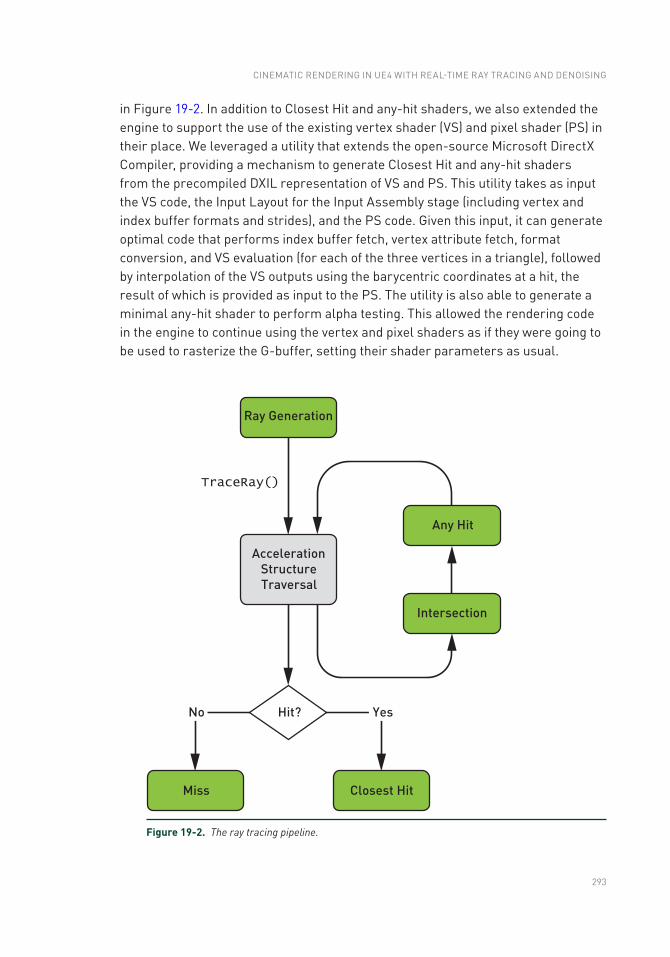
293
Figure 19-2. The ray tracing pipeline.
in Figure 19-2. In addition to Closest Hit and any-hit shaders, we also extended the engine to support the use of the existing vertex shader (VS) and pixel shader (PS) in their place. We leveraged a utility that extends the open-source Microsoft DirectX Compiler, providing a mechanism to generate Closest Hit and any-hit shaders from the precompiled DXIL representation of VS and PS. This utility takes as input the VS code, the Input Layout for the Input Assembly stage (including vertex and index buffer formats and strides), and the PS code. Given this input, it can generate optimal code that performs index buffer fetch, vertex attribute fetch, format conversion, and VS evaluation (for each of the three vertices in a triangle), followed by interpolation of the VS outputs using the barycentric coordinates at a hit, the result of which is provided as input to the PS. The utility is also able to generate a minimal any-hit shader to perform alpha testing. This allowed the rendering code in the engine to continue using the vertex and pixel shaders as if they were going to be used to rasterize the G-buffer, setting their shader parameters as usual.
CINEMATIC RENDERING IN UE4 WITH REAL-TIME RAY TRACING AND DENOISING
294
The implementation under this experimental RHI abstraction had two additional responsibilities: compiling ray tracing shaders (to a GPU-specific representation) and managing the Shader Binding Table, which points to the shader code and shader parameters that need to be used for each piece of geometry.
Compiling Ray Tracing Shaders Efficiently Prior to the introduction of RTX and DirectX Raytracing, the existing pipeline abstractions in graphics APIs (for rasterization and compute) required only a small number of shaders (1 to 5) to be provided to create a so-called pipeline state object (PSO), which encapsulates the compiled machine-specific code for the input shaders. These graphics APIs allow the creation of many of these pipeline state objects in parallel if needed, each for a different material or rendering pass. The ray tracing pipeline, however, changes this in a significant way. A ray tracing pipeline state object (RTPSO) must be created with all the shaders that may need to be executed in a given scene, such that when a ray hits any object, the system can execute the shader code associated with it, whatever that might be. In complex content in today’s games, this can easily mean thousands of shaders. Compiling thousands of ray tracing shaders into the machine code for one RTPSO could be very time consuming if done sequentially. Fortunately, both DirectX Raytracing and all other NVIDIA ray tracing APIs enabled by RTX expose the ability to compile in parallel multiple ray tracing shaders to machine code. This parallel compilation can take advantage of the multiple cores of today’s CPUs. In the experimental UE4 implementation, we used this functionality by simply scheduling separate tasks, each of which compiled a single ray tracing shader or hit group into what DXR calls a collection. Every frame, if no other shader compilation tasks were already executing, we checked if any new shaders were needed and not available. If any such shaders were found, we started a new batch of shader compilation tasks. Every frame we also checked if any prior set of shader compilation tasks had completed. If so, we created a new RTPSO, replacing the previous one. At any time, a single RTPSO is used for all DispatchRays() invocations in a frame. Any old RTPSOs replaced by a new RTPSO are scheduled for deferred deletion when no longer used by any in-flight frames. Objects for which a required shader was not yet available in the current RTPSO were removed (skipped) when building the TLAS.
The Shader Binding Table This table is a memory buffer made up of multiple records, each containing an opaque shader identifier and some shader parameters that are equivalent to what DirectX 12 calls a root table (for a Graphics Pipeline Draw or Compute Pipeline Dispatch). Since this first experimental implementation was designed to update shader parameters for every object in the scene at every frame, the Shader Binding Table management was simple, mimicking that of a command buffer. The Shader Binding Table was allocated as an N-buffered linear memory buffer, with size dictated by the number of objects in the scene. At every
RAY TRACING GEMS
295
frame we simply started writing the entire Shader Binding Table from scratch in a GPU-visible CPU-writable buffer (in an upload heap). We then enqueued GPU copies from this buffer to a GPU-local counterpart. Fence-based synchronization was used to prevent overwriting either CPU or GPU copies of the Shader Binding Table used N frames earlier.
19.2.1.3 REGISTERING GEOMETRY FOR A VARIETY OF ENGINE PRIMITIVES
To register geometry for acceleration structure construction, we had to make sure that the various primitives in UE4 had their RHI-level rtGeometry and rtObjects created for them. Typically, this requires identifying the right scope where rtGeometry and rtObjects should be created. For most primitives one can create an rtGeometry at the same scope as the vertex and index buffer geometry. This is simple to do for static triangle meshes, but for other primitives it can get more involved. For example, Particle Systems, Landscape (terrain) primitives, and Skeletal Meshes (i.e., skinned geometry, potentially using morph targets or cloth simulation) require special treatment. In UE4 we took advantage of the existing GPUSkinCache, a compute shader–based system that performs skinning at every frame into temporary GPU buffers that can be used as input to rasterization passes, acceleration structure updates, and hit shaders. It’s also important to note that each Skeletal Mesh instance needs its own separate BLAS; therefore, in this case a separate rtGeometry is needed for each instance of a Skeletal Mesh, and no instancing or sharing of these is possible, as is the case for Static Meshes.
We also experimented with support for other kinds of dynamic geometry, such as Cascade Particle Systems and the Landscape (terrain) system. Particle systems can use either particle meshes, where each particle becomes an instanced pointing to a Static Mesh’s rtGeometry, or procedurally generated triangle geometry, such as sprites or ribbons. Due to limited time, this experimental support was restricted to CPU-simulated particle systems. For the Landscape system we had some experimental support for the terrain patches, the foliage geometry, and the Spline meshes (which are meshes generated by interpolating a triangle mesh along a B-spline curve). For some of these, we relied on existing CPU code that generates the vertex geometry.
19.2.1.4 UPDATING THE RAY TRACING REPRESENTATION OF THE SCENE
At every frame, the UE4 renderer executes its Render loop body, where it performs multiple passes, such as rasterizing the G-buffer, applying direct lighting, or post- processing. We modified this loop to update the representation of the scene used
CINEMATIC RENDERING IN UE4 WITH REAL-TIME RAY TRACING AND DENOISING
296
for ray tracing purposes, which at the lowest level consists of the Shader Binding Table, associated memory buffers and resource descriptors, and the acceleration structures.
From the high-level renderer point of view, the first step involves ensuring that the shader parameters for all the objects in the scene are up to date. To do so we leveraged the existing Base Pass rendering logic, typically used to rasterize a G-buffer in the deferred shading renderer. The main difference is that for ray tracing we had to perform this loop over all the objects in the scene, not only those both inside the camera frustum and potentially visible, based on occlusion culling results. The second difference is that, instead of using the VS and PS from deferred shading G-buffer rendering, the first implementation used the VS and PS from the forward shading renderer, as that seemed like a natural fit when shading hits for reflections. A third difference is that we actually had to update shader parameters for multiple ray types, in some cases using slightly different shaders.
19.2.1.5 ITERATING OVER ALL OBJECTS
In a large scene there may be a significant amount of CPU time spent updating shader parameters for all objects. We recognized this as a potential problem and concluded that to avoid it we should aim for what people traditionally call retained mode rendering. Unlike immediate mode rendering, where at every frame the CPU resubmits many of the same commands to draw the same objects, one by one, in retained mode rendering the work performed every frame is only that needed to update anything that has changed since the last frame in a persistent representation of the scene. Retained mode rendering is a better fit for ray tracing because, unlike rasterization, in ray tracing we need global information about the entire scene. For this reason retained mode rendering is enabled by all the GPU ray tracing APIs supported by NVIDIA RTX (OptiX, DirectX Raytracing, and Vulkan Raytracing). Most real-time rendering engines today, however, are still designed around the limitations of rasterization APIs used for the last two decades, since OpenGL. As such, renderers are written to re-execute at every frame all the shader parameter setting and drawing code, ideally for as few objects as needed to render what is visible from the camera. While this same approach worked well for the small scenes we used to demonstrate real-time ray tracing, we know it will fail to scale to huge worlds. For this reason the UE4 rendering team embarked on a project to revamp the high-level renderer to aim for a more efficient retained mode rendering approach.
RAY TRACING GEMS
297
19.2.1.6 CUSTOMIZING SHADERS FOR RAY TRACED RENDERING
The second difference between ray tracing and rasterization rendering was that we had to build hit shaders from VS and PS code that were slightly customized for ray tracing purposes. The initial approach was based on the code used for forward shading in UE4, except that any logic that depends on information tied to screen-space buffers was skipped. (Side note: this implied that materials making use of nodes that access screen- space buffers do not work as expected with ray tracing. Such materials should be avoided when combining rasterization and ray tracing.) While our initial implementation used hit shaders based on UE4’s forward-rendering shaders, over time we refactored the shader code such that the hit shaders looked closer to the shaders used for G-buffer rendering in deferred shading. In this new mode all the dynamic lighting was performed in the ray generation shader instead of the hit shader. This reduced the size and complexity of hit shaders, avoiding the execution of nested TraceRay() calls in hit shaders, and allowed us to modify the lighting code for ray traced shading with much- reduced iteration times, thanks to not having to wait for the rebuilding of thousands of material pixel shaders. In addition to this change, we also optimized the VS code by ensuring we used the position computed from the ray information at a hit (origin + t * direction), thus avoiding memory loads and computation associated with position in the VS. Furthermore, where possible, we moved computation from the VS to the PS, such as when computing the transformed normal and tangent. Overall, this reduced the VS code to mostly data fetching and format conversion.
19.2.1.7 BATCH COMMIT OF SHADER PARAMETERS OF MULTIPLE RAY TYPES
The third difference, updating parameters for multiple ray types, meant that in some cases we had to loop over all the objects in the scene multiple times, if one of the ray types required a totally separate set of VS and PS. In some cases, though, we were able to significantly reduce the overhead of additional ray types. For example, we were able to handle the update of the two most common ray types, Material Evaluation and Any Hit Shadow, by allowing the RHI abstraction to commit shader parameters for multiple ray types at the same time, when these can use hit shaders that have compatible shader parameters. This requirement was guaranteed by the DirectX Compiler utility that transforms VS and PS pairs to hit shaders, as it ensured that the VS and PS parameter layout is the same for both the Closest Hit shader and the any-hit shader (since both were generated from the same VS and PS pair). Given this and the fact that the Any Hit Shadow ray type is simply using the same any-hit shader as the Material Evaluation ray type combined with a null Closest Hit shader, it was trivial to use the same Shader Binding Table record data for both ray types, but with different Shader Identifiers.
CINEMATIC RENDERING IN UE4 WITH REAL-TIME RAY TRACING AND DENOISING
298
19.2.1.8 UPDATING INSTANCE TRANSFORMATION
During the process of filling the Shader Binding Table records, we also took care of recording their offset in the associated rtObject. This information needs to be provided to the TLAS build operation, as it is used by the DXR implementation to decide what hit shaders to execute and with what parameters. In addition to updating all the shader parameters, we must also update the instance transform and flags associated with every rtObject. This is done in a separate loop, prior to updating the shader parameters. The instance-level flags allow, among other things, control of masking and backface culling logic. Masking bits are used in UE4 to implement support for lighting channels, which allow artists to restrict specific sets of lights to interacting with only specific sets of objects. Backface culling bits are used to ensure that rasterizing and ray tracing results match visually (culling is not as likely to be a performance optimization for ray tracing as it is for rasterizing).
19.2.1.9 BUILDING ACCELERATION STRUCTURES
After updating all the ray tracing shader parameters, the rtObject transforms, and the culling and masking bits, the Shader Binding Table containing hit shaders is ready, and all the rtObjects know their corresponding Shader Binding Table records. At this point we move to the next step, which is scheduling the build or update of any bottom- level acceleration structures, as well as the rebuild of the TLAS. In the experimental implementation this step also takes care of deferred allocation of memory associated with acceleration structures. One important optimization in this phase is to ensure that any resource transition barriers that are needed after BLAS updates are deferred to be executed right before the TLAS build, instead of executing these right after each BLAS update. Deferral is important because each of these transition barriers is a synchronization step on the GPU. Having the transitions coalesced into a single point in the command buffer avoids redundant synchronization that would otherwise cause the GPU to frequently become idle. By coalescing the transitions, we perform this synchronization once, after all the BLAS updates, and allow multiple BLAS updates, potentially for many small triangle meshes, to overlap while running on the GPU.
19.2.1.10 MISS SHADERS
Our use of Miss shaders is limited. Despite exposing Miss shaders at the RHI level, we never used them from the engine side of the RHI, and we relied on the RHI implementation preinitializing a set of identical default Miss shaders (one per ray type) that simply initialized a HitT value in the payload to a specific negative value, as a way to indicate that a ray had not hit anything.
RAY TRACING GEMS
299
19.2.2 PHASE 2
After accumulating experience during the creation of two high-end ray tracing demos, we were in the position to work on a big refactoring that could make it possible to transition from code being project-specific to something that scales well for the needs of all UE4 users. One of the ultimate goals of this phase was to move the UE4 rendering system from immediate to retained mode. This led to higher efficiency, as only objects that changed at a given frame are effectively updated. Because of limitations of rasterization pipelines, UE4 was initially written following an immediate mode style. However, this would represent a serious limitation for ray tracing large scenes, since it always updates all the objects for each frame even though most of the time only a small portion changed. So, moving to a retained mode style was one of the key accomplishments of this phase.
With the ultimate goal of making it possible to integrate ray tracing in any platform in the future, we divided the requirements in different tiers, to understand what was needed for supporting each feature and how we could face limitations of any particular device without sacrificing functionality when more advance hardware was present.
19.2.2.1 TIER 1
Tier 1 describes the lowest level of functionality required to integrate basic ray tracing capabilities and is like existing ray tracing APIs such as Radeon Rays or Metal Performance Shaders. The input is a buffer that contains ray information (origin, direction), and the shader output is a buffer that contains intersection results. There is no built-in TraceRay intrinsic function nor are there any hit shaders available in this tier. Tier 1 is a good fit for implementing simple ray tracing effects such as opaque shadows or ambient occlusion, but going beyond these is challenging and requires complex changes in the code that introduce restrictions and make it difficult to achieve good execution efficiency.
19.2.2.2 TIER 2
Tier 2 supports ray generation shaders, which can call a TraceRay intrinsic function whose output is available immediately after the trace call. This level of functionality also supports dynamic shader dispatch, which is abstracted using RTPSOs and Shader Binding Tables. Tier 2 does not support recursive ray tracing, so new rays cannot be spawned from hit shaders. During phase 1 we found that this was not a big limitation in practice, and it had the positive side effect of reducing the size and complexity of hit shaders.
CINEMATIC RENDERING IN UE4 WITH REAL-TIME RAY TRACING AND DENOISING
300
Tier 2 makes it possible to implement most of the goals defined in the ray tracing integration in UE4. Therefore, the design of the UE4 ray tracing pipeline has been done assuming Tier 2 capabilities.
19.2.2.3 TIER 3
Tier 3 closely follows the DXR specification. It supports all Tier 2 features and recursive calls with a predefined maximum depth. It also supports tracing rays from other shader types beyond ray generation shaders, as well as advanced features, such as customizable acceleration structure traversal. Tier 3 is the most powerful set of capabilities to date, and it enables integration of advanced ray tracing features from offline rendering, e.g., photon mapping and irradiance caching, in a modular way. The ray tracing integration in UE4 has been designed to make use of Tier 3 capabilities when the hardware supports it.
19.3 REAL-TIME RAY TRACING AND DENOISING
In addition to lessons learned from the ray tracing integration in UE4, the initial experimental phase was essential to explore the possibilities of real-time ray tracing. We started with mirror reflections and hard shadows, continued by adding denoising to approximate glossy reflections and area light shadows from a limited ray budget, and then added ambient occlusion, diffuse global illumination, and translucency.
We note that rasterization-based renderers (both offline and real-time) often split the rendering equation into multiple segments of light paths and deal with each segment separately. For example, a separate pass is performed for screen-space reflection, and another pass for direct lighting. This is less commonly used in ray tracing renderers, in particular offline path tracers, which instead render by accumulating tens, hundreds, or thousands of light paths.
Some ray tracing renderers use techniques to improve convergence or interactivity, e.g., virtual point lights (instant radiosity [6]), path space filtering [1], and a plethora of denoising algorithms. For an overview of recent denoising techniques for Monte Carlo rendering, please refer to Zwicker et al’s [14] excellent state-of-the-art report.
Zimmer et al. [13] split the entire ray tree into separate buffers and applied denoising filters to each buffer before compositing the final frame. In our scenario, we follow a similar approach, splitting the light paths that emerge when we try to solve the rendering equation. We apply custom filters for results from different ray types, e.g., shadow, reflection, and diffuse rays. We use a small number of rays per pixel for each effect and denoise them aggressively to make up for the insufficient
RAY TRACING GEMS
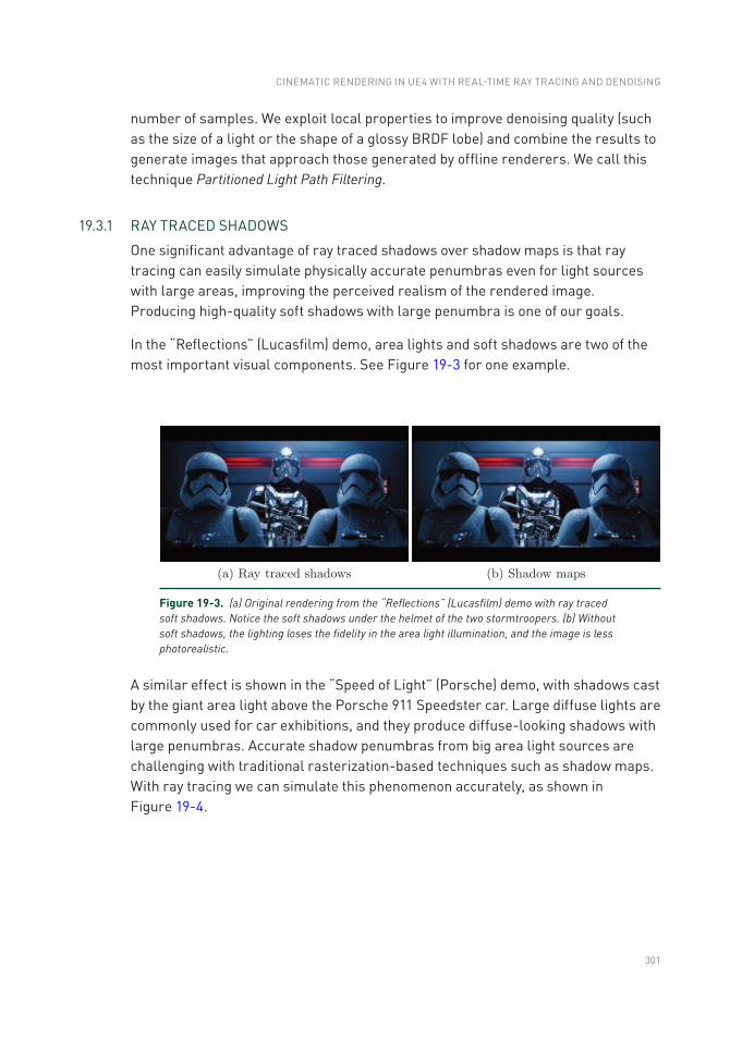
301
number of samples. We exploit local properties to improve denoising quality (such as the size of a light or the shape of a glossy BRDF lobe) and combine the results to generate images that approach those generated by offline renderers. We call this technique Partitioned Light Path Filtering.
19.3.1 RAY TRACED SHADOWS
One significant advantage of ray traced shadows over shadow maps is that ray tracing can easily simulate physically accurate penumbras even for light sources with large areas, improving the perceived realism of the rendered image. Producing high-quality soft shadows with large penumbra is one of our goals.
In the “Reflections” (Lucasfilm) demo, area lights and soft shadows are two of the most important visual components. See Figure 19-3 for one example.
Figure 19-3. (a) Original rendering from the “Reflections” (Lucasfilm) demo with ray traced soft shadows. Notice the soft shadows under the helmet of the two stormtroopers. (b) Without soft shadows, the lighting loses the fidelity in the area light illumination, and the image is less photorealistic.
A similar effect is shown in the “Speed of Light” (Porsche) demo, with shadows cast by the giant area light above the Porsche 911 Speedster car. Large diffuse lights are commonly used for car exhibitions, and they produce diffuse-looking shadows with large penumbras. Accurate shadow penumbras from big area light sources are challenging with traditional rasterization-based techniques such as shadow maps. With ray tracing we can simulate this phenomenon accurately, as shown in Figure 19-4.
CINEMATIC RENDERING IN UE4 WITH REAL-TIME RAY TRACING AND DENOISING
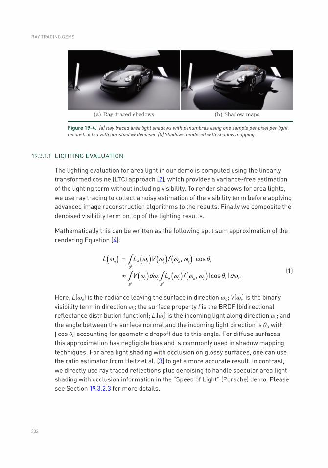
302
19.3.1.1 LIGHTING EVALUATION
The lighting evaluation for area light in our demo is computed using the linearly transformed cosine (LTC) approach [2], which provides a variance-free estimation of the lighting term without including visibility. To render shadows for area lights, we use ray tracing to collect a noisy estimation of the visibility term before applying advanced image reconstruction algorithms to the results. Finally we composite the denoised visibility term on top of the lighting results.
Mathematically this can be written as the following split sum approximation of the rendering Equation [4]:
( ) ( ) ( ) ( )
( ) ( ) ( )
o d i i o i iS
i i d i o i i iS S
L L V f
V d L f d2
2 2
,
.
cos
, cos
w w w w w q
w w w w w q w
ò
ò ò
=
»
∣ ∣
∣ ∣
(1)
Here, L(ωo) is the radiance leaving the surface in direction ωo; V(ωi) is the binary visibility term in direction ωi; the surface property f is the BRDF (bidirectional reflectance distribution function); Li(ωi) is the incoming light along direction ωi; and the angle between the surface normal and the incoming light direction is θi, with ∣ cos θi∣ accounting for geometric dropoff due to this angle. For diffuse surfaces, this approximation has negligible bias and is commonly used in shadow mapping techniques. For area light shading with occlusion on glossy surfaces, one can use the ratio estimator from Heitz et al. [3] to get a more accurate result. In contrast, we directly use ray traced reflections plus denoising to handle specular area light shading with occlusion information in the “Speed of Light” (Porsche) demo. Please see Section 19.3.2.3 for more details.
Figure 19-4. (a) Ray traced area light shadows with penumbras using one sample per pixel per light, reconstructed with our shadow denoiser. (b) Shadows rendered with shadow mapping.
RAY TRACING GEMS
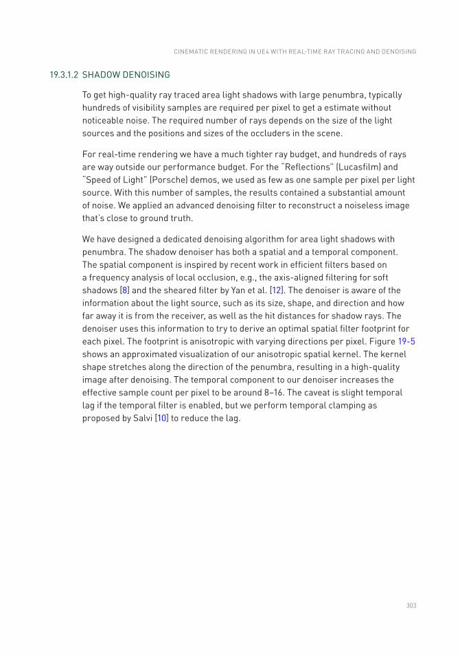
303
19.3.1.2 SHADOW DENOISING
To get high-quality ray traced area light shadows with large penumbra, typically hundreds of visibility samples are required per pixel to get a estimate without noticeable noise. The required number of rays depends on the size of the light sources and the positions and sizes of the occluders in the scene.
For real-time rendering we have a much tighter ray budget, and hundreds of rays are way outside our performance budget. For the “Reflections” (Lucasfilm) and “Speed of Light” (Porsche) demos, we used as few as one sample per pixel per light source. With this number of samples, the results contained a substantial amount of noise. We applied an advanced denoising filter to reconstruct a noiseless image that’s close to ground truth.
We have designed a dedicated denoising algorithm for area light shadows with penumbra. The shadow denoiser has both a spatial and a temporal component. The spatial component is inspired by recent work in efficient filters based on a frequency analysis of local occlusion, e.g., the axis-aligned filtering for soft shadows [8] and the sheared filter by Yan et al. [12]. The denoiser is aware of the information about the light source, such as its size, shape, and direction and how far away it is from the receiver, as well as the hit distances for shadow rays. The denoiser uses this information to try to derive an optimal spatial filter footprint for each pixel. The footprint is anisotropic with varying directions per pixel. Figure 19-5 shows an approximated visualization of our anisotropic spatial kernel. The kernel shape stretches along the direction of the penumbra, resulting in a high-quality image after denoising. The temporal component to our denoiser increases the effective sample count per pixel to be around 8–16. The caveat is slight temporal lag if the temporal filter is enabled, but we perform temporal clamping as proposed by Salvi [10] to reduce the lag.
CINEMATIC RENDERING IN UE4 WITH REAL-TIME RAY TRACING AND DENOISING
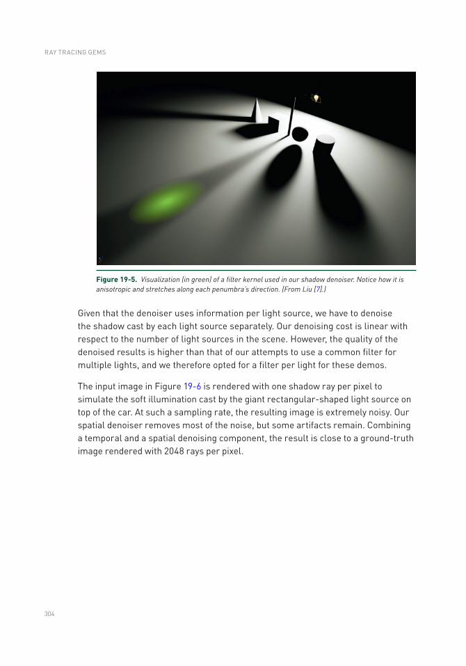
304
Given that the denoiser uses information per light source, we have to denoise the shadow cast by each light source separately. Our denoising cost is linear with respect to the number of light sources in the scene. However, the quality of the denoised results is higher than that of our attempts to use a common filter for multiple lights, and we therefore opted for a filter per light for these demos.
The input image in Figure 19-6 is rendered with one shadow ray per pixel to simulate the soft illumination cast by the giant rectangular-shaped light source on top of the car. At such a sampling rate, the resulting image is extremely noisy. Our spatial denoiser removes most of the noise, but some artifacts remain. Combining a temporal and a spatial denoising component, the result is close to a ground-truth image rendered with 2048 rays per pixel.
Figure 19-5. Visualization (in green) of a filter kernel used in our shadow denoiser. Notice how it is anisotropic and stretches along each penumbra’s direction. (From Liu [7].)
RAY TRACING GEMS
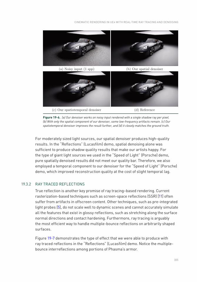
305
Figure 19-6. (a) Our denoiser works on noisy input rendered with a single shadow ray per pixel. (b) With only the spatial component of our denoiser, some low- frequency artifacts remain. (c) Our spatiotemporal denoiser improves the result further, and (d) it closely matches the ground truth.
For moderately sized light sources, our spatial denoiser produces high-quality results. In the “Reflections” (Lucasfilm) demo, spatial denoising alone was sufficient to produce shadow quality results that make our artists happy. For the type of giant light sources we used in the “Speed of Light” (Porsche) demo, pure spatially denoised results did not meet our quality bar. Therefore, we also employed a temporal component to our denoiser for the “Speed of Light” (Porsche) demo, which improved reconstruction quality at the cost of slight temporal lag.
19.3.2 RAY TRACED REFLECTIONS
True reflection is another key promise of ray tracing–based rendering. Current rasterization-based techniques such as screen-space reflections (SSR) [11] often suffer from artifacts in offscreen content. Other techniques, such as pre-integrated light probes [5], do not scale well to dynamic scenes and cannot accurately simulate all the features that exist in glossy reflections, such as stretching along the surface normal directions and contact hardening. Furthermore, ray tracing is arguably the most efficient way to handle multiple-bounce reflections on arbitrarily shaped surfaces.
Figure 19-7 demonstrates the type of effect that we were able to produce with ray traced reflections in the “Reflections” (Lucasfilm) demo. Notice the multiple-bounce interreflections among portions of Phasma’s armor.
CINEMATIC RENDERING IN UE4 WITH REAL-TIME RAY TRACING AND DENOISING
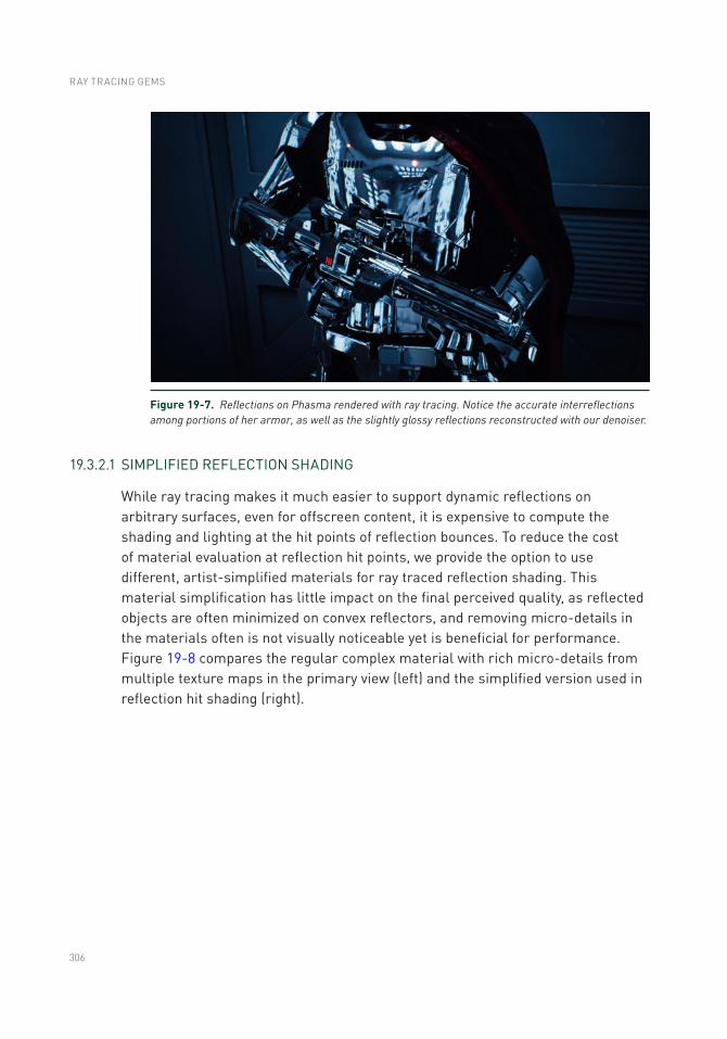
306
19.3.2.1 SIMPLIFIED REFLECTION SHADING
While ray tracing makes it much easier to support dynamic reflections on arbitrary surfaces, even for offscreen content, it is expensive to compute the shading and lighting at the hit points of reflection bounces. To reduce the cost of material evaluation at reflection hit points, we provide the option to use different, artist-simplified materials for ray traced reflection shading. This material simplification has little impact on the final perceived quality, as reflected objects are often minimized on convex reflectors, and removing micro-details in the materials often is not visually noticeable yet is beneficial for performance. Figure 19-8 compares the regular complex material with rich micro- details from multiple texture maps in the primary view (left) and the simplified version used in reflection hit shading (right).
Figure 19-7. Reflections on Phasma rendered with ray tracing. Notice the accurate interreflections among portions of her armor, as well as the slightly glossy reflections reconstructed with our denoiser.
RAY TRACING GEMS
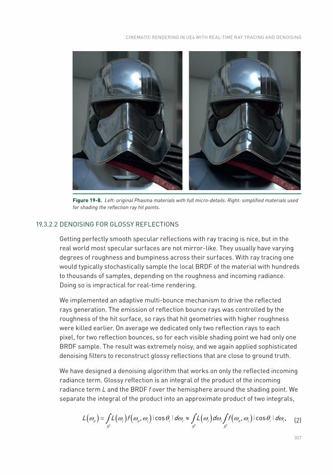
307
19.3.2.2 DENOISING FOR GLOSSY REFLECTIONS
Getting perfectly smooth specular reflections with ray tracing is nice, but in the real world most specular surfaces are not mirror-like. They usually have varying degrees of roughness and bumpiness across their surfaces. With ray tracing one would typically stochastically sample the local BRDF of the material with hundreds to thousands of samples, depending on the roughness and incoming radiance. Doing so is impractical for real-time rendering.
We implemented an adaptive multi-bounce mechanism to drive the reflected rays generation. The emission of reflection bounce rays was controlled by the roughness of the hit surface, so rays that hit geometries with higher roughness were killed earlier. On average we dedicated only two reflection rays to each pixel, for two reflection bounces, so for each visible shading point we had only one BRDF sample. The result was extremely noisy, and we again applied sophisticated denoising filters to reconstruct glossy reflections that are close to ground truth.
We have designed a denoising algorithm that works on only the reflected incoming radiance term. Glossy reflection is an integral of the product of the incoming radiance term L and the BRDF f over the hemisphere around the shading point. We separate the integral of the product into an approximate product of two integrals,
( ) ( ) ( ) ( ) ( )o i o i i i i i o i i iS S S
L L f d L d f d2 2 2
, cos , cos ,w w w w q w w w w w q wò ò ò= »∣ ∣ ∣ ∣ (2)
Figure 19-8. Left: original Phasma materials with full micro-details. Right: simplified materials used for shading the reflection ray hit points.
CINEMATIC RENDERING IN UE4 WITH REAL-TIME RAY TRACING AND DENOISING
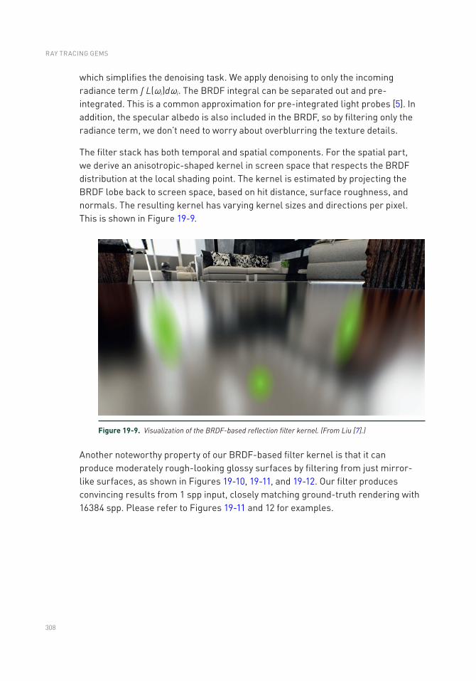
308
which simplifies the denoising task. We apply denoising to only the incoming radiance term ∫ L(ωi)dωi. The BRDF integral can be separated out and pre-integrated. This is a common approximation for pre-integrated light probes [5]. In addition, the specular albedo is also included in the BRDF, so by filtering only the radiance term, we don’t need to worry about overblurring the texture details.
The filter stack has both temporal and spatial components. For the spatial part, we derive an anisotropic-shaped kernel in screen space that respects the BRDF distribution at the local shading point. The kernel is estimated by projecting the BRDF lobe back to screen space, based on hit distance, surface roughness, and normals. The resulting kernel has varying kernel sizes and directions per pixel. This is shown in Figure 19-9.
Figure 19-9. Visualization of the BRDF-based reflection filter kernel. (From Liu [7].)
Another noteworthy property of our BRDF-based filter kernel is that it can produce moderately rough-looking glossy surfaces by filtering from just mirror-like surfaces, as shown in Figures 19-10, 19-11, and 19-12. Our filter produces convincing results from 1 spp input, closely matching ground-truth rendering with 16384 spp. Please refer to Figures 19-11 and 12 for examples.
RAY TRACING GEMS
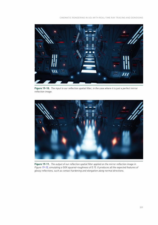
309
Figure 19-10. The input to our reflection spatial filter, in the case where it is just a perfect mirror reflection image.
Figure 19-11. The output of our reflection spatial filter applied on the mirror reflection image in Figure 19-10, simulating a GGX squared-roughness of 0.15. It produces all the expected features of glossy reflections, such as contact hardening and elongation along normal directions.
CINEMATIC RENDERING IN UE4 WITH REAL-TIME RAY TRACING AND DENOISING
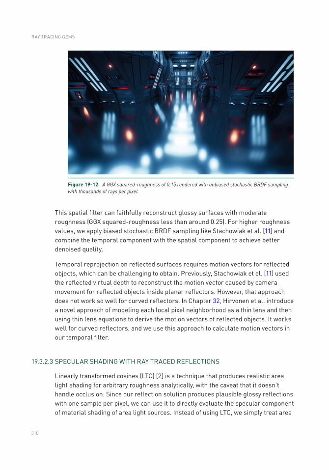
310
Figure 19-12. A GGX squared-roughness of 0.15 rendered with unbiased stochastic BRDF sampling with thousands of rays per pixel.
This spatial filter can faithfully reconstruct glossy surfaces with moderate roughness (GGX squared-roughness less than around 0.25). For higher roughness values, we apply biased stochastic BRDF sampling like Stachowiak et al. [11] and combine the temporal component with the spatial component to achieve better denoised quality.
Temporal reprojection on reflected surfaces requires motion vectors for reflected objects, which can be challenging to obtain. Previously, Stachowiak et al. [11] used the reflected virtual depth to reconstruct the motion vector caused by camera movement for reflected objects inside planar reflectors. However, that approach does not work so well for curved reflectors. In Chapter 32, Hirvonen et al. introduce a novel approach of modeling each local pixel neighborhood as a thin lens and then using thin lens equations to derive the motion vectors of reflected objects. It works well for curved reflectors, and we use this approach to calculate motion vectors in our temporal filter.
19.3.2.3 SPECULAR SHADING WITH RAY TRACED REFLECTIONS
Linearly transformed cosines (LTC) [2] is a technique that produces realistic area light shading for arbitrary roughness analytically, with the caveat that it doesn’t handle occlusion. Since our reflection solution produces plausible glossy reflections with one sample per pixel, we can use it to directly evaluate the specular component of material shading of area light sources. Instead of using LTC, we simply treat area
RAY TRACING GEMS
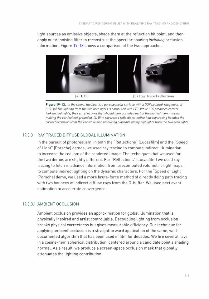
311
light sources as emissive objects, shade them at the reflection hit point, and then apply our denoising filter to reconstruct the specular shading including occlusion information. Figure 19-13 shows a comparison of the two approaches.
19.3.3 RAY TRACED DIFFUSE GLOBAL ILLUMINATION
In the pursuit of photorealism, in both the “Reflections” (Lucasfilm) and the “Speed of Light” (Porsche) demos, we used ray tracing to compute indirect illumination to increase the realism of the rendered image. The techniques that we used for the two demos are slightly different. For “Reflections” (Lucasfilm) we used ray tracing to fetch irradiance information from precomputed volumetric light maps to compute indirect lighting on the dynamic characters. For the “Speed of Light” (Porsche) demo, we used a more brute- force method of directly doing path tracing with two bounces of indirect diffuse rays from the G-buffer. We used next event estimation to accelerate convergence.
19.3.3.1 AMBIENT OCCLUSION
Ambient occlusion provides an approximation for global illumination that is physically inspired and artist controllable. Decoupling lighting from occlusion breaks physical correctness but gives measurable efficiency. Our technique for applying ambient occlusion is a straightforward application of the same, well-documented algorithm that has been used in film for decades. We fire several rays, in a cosine-hemispherical distribution, centered around a candidate point’s shading normal. As a result, we produce a screen-space occlusion mask that globally attenuates the lighting contribution.
Figure 19-13. In the scene, the floor is a pure specular surface with a GGX squared-roughness of 0.17. (a) The lighting from the two area lights is computed with LTC. While LTC produces correct-looking highlights, the car reflections that should have occluded part of the highlight are missing, making the car feel not grounded. (b) With ray traced reflections, notice how ray tracing handles the correct occlusion from the car while also producing plausible glossy highlights from the two area lights.
CINEMATIC RENDERING IN UE4 WITH REAL-TIME RAY TRACING AND DENOISING
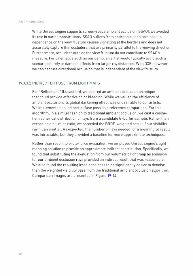
312
While Unreal Engine supports screen-space ambient occlusion (SSAO), we avoided its use in our demonstrations. SSAO suffers from noticeable shortcomings. Its dependence on the view frustum causes vignetting at the borders and does not accurately capture thin occluders that are primarily parallel to the viewing direction. Furthermore, occluders outside the view frustum do not contribute to SSAO’s measure. For cinematics such as our demo, an artist would typically avoid such a scenario entirely or dampen effects from larger ray distances. With DXR, however, we can capture directional occlusion that is independent of the view frustum.
19.3.3.2 INDIRECT DIFFUSE FROM LIGHT MAPS
For “Reflections” (Lucasfilm), we desired an ambient occlusion technique that could provide effective color bleeding. While we valued the efficiency of ambient occlusion, its global darkening effect was undesirable to our artists. We implemented an indirect diffuse pass as a reference comparison. For this algorithm, in a similar fashion to traditional ambient occlusion, we cast a cosine-hemispherical distribution of rays from a candidate G-buffer sample. Rather than recording a hit-miss ratio, we recorded the BRDF-weighted result if our visibility ray hit an emitter. As expected, the number of rays needed for a meaningful result was intractable, but they provided a baseline for more approximate techniques.
Rather than resort to brute-force evaluation, we employed Unreal Engine’s light mapping solution to provide an approximate indirect contribution. Specifically, we found that substituting the evaluation from our volumetric light map as emission for our ambient occlusion rays provided an indirect result that was reasonable. We also found the resulting irradiance pass to be significantly easier to denoise than the weighted visibility pass from the traditional ambient occlusion algorithm. Comparison images are presented in Figure 19-14.
RAY TRACING GEMS
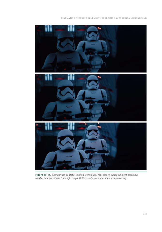
313
Figure 19-14. Comparison of global lighting techniques. Top: screen-space ambient occlusion. Middle: indirect diffuse from light maps. Bottom: reference one- bounce path tracing.
CINEMATIC RENDERING IN UE4 WITH REAL-TIME RAY TRACING AND DENOISING
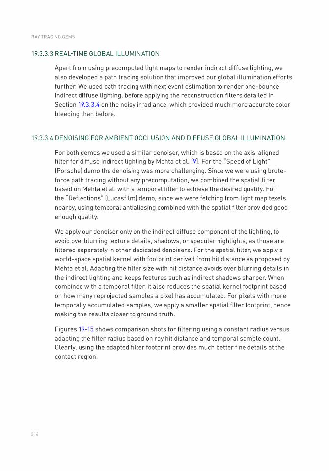
314
19.3.3.3 REAL-TIME GLOBAL ILLUMINATION
Apart from using precomputed light maps to render indirect diffuse lighting, we also developed a path tracing solution that improved our global illumination efforts further. We used path tracing with next event estimation to render one-bounce indirect diffuse lighting, before applying the reconstruction filters detailed in Section 19.3.3.4 on the noisy irradiance, which provided much more accurate color bleeding than before.
19.3.3.4 DENOISING FOR AMBIENT OCCLUSION AND DIFFUSE GLOBAL ILLUMINATION
For both demos we used a similar denoiser, which is based on the axis-aligned filter for diffuse indirect lighting by Mehta et al. [9]. For the “Speed of Light” (Porsche) demo the denoising was more challenging. Since we were using brute-force path tracing without any precomputation, we combined the spatial filter based on Mehta et al. with a temporal filter to achieve the desired quality. For the “Reflections” (Lucasfilm) demo, since we were fetching from light map texels nearby, using temporal antialiasing combined with the spatial filter provided good enough quality.
We apply our denoiser only on the indirect diffuse component of the lighting, to avoid overblurring texture details, shadows, or specular highlights, as those are filtered separately in other dedicated denoisers. For the spatial filter, we apply a world-space spatial kernel with footprint derived from hit distance as proposed by Mehta et al. Adapting the filter size with hit distance avoids over blurring details in the indirect lighting and keeps features such as indirect shadows sharper. When combined with a temporal filter, it also reduces the spatial kernel footprint based on how many reprojected samples a pixel has accumulated. For pixels with more temporally accumulated samples, we apply a smaller spatial filter footprint, hence making the results closer to ground truth.
Figures 19-15 shows comparison shots for filtering using a constant radius versus adapting the filter radius based on ray hit distance and temporal sample count. Clearly, using the adapted filter footprint provides much better fine details at the contact region.
RAY TRACING GEMS

315
Figure 19-15. Indirect lighting filtered with (a) a uniform world-space radius and (b) an adaptive kernel. The adaptive kernel size is based on average ray hit distance and accumulated temporal sample count.
The same idea also helps with ray traced ambient occlusion denoising. In Figure 19- 16 we compare (a) denoised ray traced ambient occlusion with a constant world-space radius, with (b) denoised ambient occlusion using adaptive kernel radius guided with hit distance and temporal sample-count.
It is clear again that using adaptive filter sizes leads to better-preserved contact details in the denoised ambient occlusion.
19.3.4 RAY TRACED TRANSLUCENCY
The “Speed of Light” (Porsche) demo presented a number of new challenges. The most obvious initial challenge to the team was that of rendering glass. Traditional methods for rendering real-time translucency conflict with deferred rendering algorithms. Often, developers are required to render translucent geometry in a separate forward pass and composite the result over the main deferred rendering. Techniques that can be applied to deferred rendering are often unsuitable for translucent geometry, creating incompatibilities that make integration of translucent and opaque geometry difficult.
Figure 19-16. Ambient occlusion filtered with (a) a uniform world-space radius and (b) an adaptive kernel. The adaptive kernel size is based on average ray hit distance and accumulated temporal sample count.
CINEMATIC RENDERING IN UE4 WITH REAL-TIME RAY TRACING AND DENOISING

316
Fortunately, ray tracing provides a natural framework for representing translucency. With ray tracing, translucent geometry can easily be combined with deferred rendering in a way that unifies geometry submission. It provides arbitrary translucent depth complexity as well as the capability to correctly model refraction and absorption.
19.3.4.1 RAY GENERATION
Our implementation of ray traced translucency in Unreal Engine uses a separate ray tracing pass similar to the one used for ray traced reflections. In fact, most of the shader code is shared between these two passes. There are, however, a few small nuanced differences between how the two behave. The first one is the use of early-ray termination to prevent unnecessary traversal through the scene once the throughput of the ray is close to zero; i.e., if traversed farther, its contribution is negligible. Another difference is that translucent rays are traced with a maximum ray length that prevents hitting the opaque geometry that has already being fully shaded and stored at the corresponding pixel. However, if refraction is performed, a translucent hit may result in a new ray in an arbitrary direction, and this new ray or its descendants may hit opaque geometry, which will need to be shaded. Before we perform any lighting on such opaque hits, we perform a reprojection of the opaque hit point to the screen buffer, and if valid data are found after this reprojection step, they are used instead. This simple trick allowed us to take advantage of the higher visual quality achieved when performing all the ray traced lighting and denoising on opaque geometry in the G-buffer. This can work for some limited amount of refraction, although the results can be incorrect due to specular lighting being computed with the wrong incoming direction in such cases.
Another key difference with the reflection pass is the ability for translucent rays to recursively generate reflection rays after hitting subsequent interfaces. This was not completely straightforward to implement using HLSL due to the lack of support for recursion in the language. By recursion we do not mean the ability to trace rays from a hit shader, but the ability for a simple HLSL function to call itself. This is simply not allowed in HLSL, but it is desirable when implementing a Whitted-style ray tracing algorithm, as we did in this case. To work around this limitation of HLSL, we instantiated the same code into two functions with different names. We effectively moved the relevant function code into a separate file and included this file twice, surrounded by preprocessor macros that set the function name each time, resulting in two different instantiations of the same function code with different names. We then made one of the two function instantiations call the other one, thus allowing us to effectively have recursion with a hard-coded limit of one level. The resulting implementation permits translucent paths, with optional
RAY TRACING GEMS
317
refraction, where each hit along the path could trace “recursive” reflection rays in addition to shadow rays. Reflections traced off translucent surfaces along this path could potentially bounce up to a selected number of times. However, if at any of these bounces a translucent surface was hit, we did not allow additional recursive reflection rays to be traced.
Homogeneous volumetric absorption following the Beer-Lambert law was added to our translucency pass to model thick glass and to approximate the substrate. To correctly model homogeneous bounded volumes, additional constraints were placed on the geometry. Ray traversal was modified to explicitly trace against both frontfacing and backfacing polygons to overcome issues with intersecting, non-manifold geometry. The improved visual realism was considered not worth the slight added cost for the “Speed of Light” (Porsche) demo and was not included in its final version.
19.4 CONCLUSIONS
The recent introduction of dedicated hardware for ray tracing acceleration and the addition of ray tracing support in graphics APIs encouraged us to be innovative and experiment with a new way of hybrid rendering, combining rasterization and ray tracing. We went through the engineering practice of integrating ray tracing in Unreal Engine 4, a commercial-grade game engine. We invented innovative reconstruction filters for rendering stochastic effects such as glossy reflections, soft shadows, ambient occlusion, and diffuse indirect illumination with as few as a single path per pixel, making these expensive effects more practical for use in real time. We have successfully used hybrid rendering to create two cinematic-quality demos.
ACKNOWLEDGMENTS
As a historical note, Epic Games, in collaboration with NVIDIA and ILMxLAB, gave the first public demonstration of real-time ray tracing in Unreal Engine during Epic’s “State of Unreal” opening session at Game Developers Conference in March 2018. The demo showed Star Wars characters from The Force Awakens and The Last Jedi built with Unreal Engine 4. It was originally run on NVIDIA’s RTX technology for Volta GPUs via Microsoft’s DirectX Raytracing API.
Mohen Leo (ILMxLAB) joined Marcus Wassmer and Jerome Platteaux from Epic Games in the development and presentation of the techniques used in that demo. ILMxLAB is Lucasfilm’s immersive entertainment division, known best for their work on CARNE y ARENA, Star Wars: Secrets of the Empire, and the upcoming Vader Immortal: A Star Wars VR Series. Many others who have worked or consulted
CINEMATIC RENDERING IN UE4 WITH REAL-TIME RAY TRACING AND DENOISING
318
on the ray tracing content and implementation for UE4 include Guillaume Abadie, Francois Antoine, Louis Bavoil, Alexander Bogomjakov, Rob Bredow, Uriel Doyon, Maksim Eisenstein, Judah Graham, Evan Hart, Jon Hasselgren, Matthias Hollander, John Jack, Matthew Johnson, Brian Karis, Kim Libreri, Simone Lombardo, Adam Marrs, Gavin Moran, Jacob Munkberg, Yuriy O’Donnell, Min Oh, Jacopo Pantaleoni, Arne Schober, Jon Story, Peter Sumanaseni, Minjie Wu, Chris Wyman, and Michael Zhang.
Star Wars images are used courtesy of Lucasfilm.
REFERENCES
[1] Binder, N., Fricke, S., and Keller, A. Fast Path Space Filtering by Jittered Spatial Hashing. In ACM SIGGRAPH Talks (2018), pp. 71:1–71:2.
[2] Eric Heitz, Jonathan Dupuy, S. H., and Neubelt, D. Real-Time Polygonal-Light Shading with Linearly Transformed Cosines. ACM Transactions on Graphics 35, 4 (2017), 41:1–41:8.
[3] Heitz, E., Hill, S., and McGuire, M. Combining Analytic Direct Illumination and Stochastic Shadows. In Symposium on Interactive 3D Graphics and Games (2018), pp. 2:1–2:11.
[4] Kajiya, J. T. The Rendering Equation. Computer Graphics (SIGGRAPH) (1986), 143–150.
[5] Karis, B. Real Shading in Unreal Engine 4. Physically Based Shading in Theory and Practice, SIGGRAPH Courses, August 2013.
[6] Keller, A. Instant Radiosity. In Proceedings of SIGGRAPH (1997), pp. 49–56.
[7] Liu, E. Low Sample Count Ray Tracing with NVIDIA’s Ray Tracing Denoisers. Real- Time Ray Tracing, SIGGRAPH Courses, August 2018.
[8] Mehta, S., Wang, B., and Ramamoorthi, R. Axis-Aligned Filtering for Interactive Sampled Soft Shadows. ACM Transactions on Graphics 31, 6 (Nov 2012), 163:1–163:10.
[9] Mehta, S. U., Wang, B., Ramamoorthi, R., and Durand, F. Axis-aligned Filtering for Interactive Physically-based Diffuse Indirect Lighting. ACM Transactions on Graphics 32, 4 (July 2013), 96:1–96:12.
[10] Salvi, M. An Excursion in Temporal Supersampling. From the Lab Bench: Real-Time Rendering Advances from NVIDIA Research, Game Developers Conference, 2016.
[11] Stachowiak, T. Stochastic Screen Space Reflections. Advances in Real-Time Rendering, SIGGRAPH Courses, 2018.
[12] Yan, L.-Q., Mehta, S. U., Ramamoorthi, R., and Durand, F. Fast 4D Sheared Filtering for Interactive Rendering of Distribution Effects. ACM Transactions on Graphics 35, 1 (2015), 7:1–7:13.
RAY TRACING GEMS

319
[13] Zimmer, H., Rousselle, F., Jakob, W., Wang, O., Adler, D., Jarosz, W., Sorkine- Hornung, O., and Sorkine-Hornung, A. Path-Space Motion Estimation and Decomposition for Robust Animation Filtering. Computer Graphics Forum 34, 4 (2015), 131–142.
[14] Zwicker, M., Jarosz, W., Lehtinen, J., Moon, B., Ramamoorthi, R., Rousselle, F., Sen, P., Soler, C., and Yoon, S.-E. Recent Advances in Adaptive Sampling and Reconstruction for Monte Carlo Rendering. Computer Graphics Forum (Proceedings of Eurographics—State of the Art Reports) 34, 2 (May 2015), 667681.
Open Access This chapter is licensed under the terms of the Creative Commons Attribution-NonCommercial-NoDerivatives 4.0 International License (http://creativecommons.org/licenses/by-nc-nd/4.0/), which permits any noncommercial use, sharing, distribution and
reproduction in any medium or format, as long as you give appropriate credit to the original author(s) and the source, provide a link to the Creative Commons license and indicate if you modified the licensed material. You do not have permission under this license to share adapted material derived from this chapter or parts of it.
The images or other third party material in this chapter are included in the chapter's Creative Commons license, unless indicated otherwise in a credit line to the material. If material is not included in the chapter's Creative Commons license and your intended use is not permitted by statutory regulation or exceeds the permitted use, you will need to obtain permission directly from the copyright holder.
CINEMATIC RENDERING IN UE4 WITH REAL-TIME RAY TRACING AND DENOISING
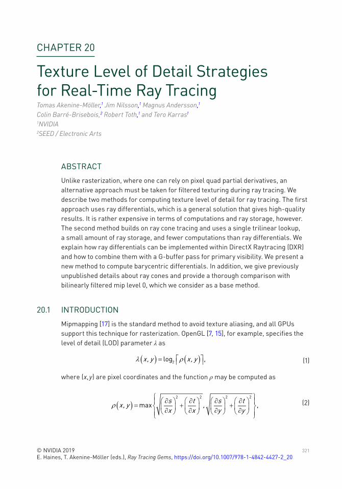
321© NVIDIA 2019 E. Haines, T. Akenine-Möller (eds.), Ray Tracing Gems, https://doi.org/10.1007/978-1-4842-4427-2_20
CHAPTER 20
Texture Level of Detail Strategies for Real-Time Ray TracingTomas Akenine-Möller,1 Jim Nilsson,1 Magnus Andersson,1 Colin Barré-Brisebois,2 Robert Toth,1 and Tero Karras1
1NVIDIA 2SEED / Electronic Arts
ABSTRACT
Unlike rasterization, where one can rely on pixel quad partial derivatives, an alternative approach must be taken for filtered texturing during ray tracing. We describe two methods for computing texture level of detail for ray tracing. The first approach uses ray differentials, which is a general solution that gives high-quality results. It is rather expensive in terms of computations and ray storage, however. The second method builds on ray cone tracing and uses a single trilinear lookup, a small amount of ray storage, and fewer computations than ray differentials. We explain how ray differentials can be implemented within DirectX Raytracing (DXR) and how to combine them with a G-buffer pass for primary visibility. We present a new method to compute barycentric differentials. In addition, we give previously unpublished details about ray cones and provide a thorough comparison with bilinearly filtered mip level 0, which we consider as a base method.
20.1 INTRODUCTION
Mipmapping [17] is the standard method to avoid texture aliasing, and all GPUs support this technique for rasterization. OpenGL [7, 15], for example, specifies the level of detail (LOD) parameter λ as
( ) ( )x, y x, y2log ,l ré ùê ú= (1)
where (x, y) are pixel coordinates and the function ρ may be computed as
( ) s t s tx, y ,x x y y
2 22 2
max ,rì üæ ö æ öæ ¶ ö æ ¶ ö ¶ ¶ï ï= + +í ýç ÷ ç ÷ç ÷ ç ÷¶ ¶ ¶ ¶è ø è ø è ø è øï ïî þ
(2)
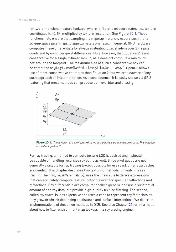
322
for two-dimensional texture lookups, where (s, t) are texel coordinates, i.e., texture coordinates (∈ [0, 1]2) multiplied by texture resolution. See Figure 20-1. These functions help ensure that sampling the mipmap hierarchy occurs such that a screen-space pixel maps to approximately one texel. In general, GPU hardware computes these differentials by always evaluating pixel shaders over 2 × 2 pixel quads and by using per-pixel differences. Note, however, that Equation 2 is not conservative for a single trilinear lookup, as it does not compute a minimum box around the footprint. The maximum side of such a conservative box can be computed as ρ(x, y) = max(| ∂s/∂x| + | ∂s/∂y| , | ∂t/∂x| + | ∂t/∂y|). OpenGL allows use of more conservative estimates than Equation 2, but we are unaware of any such approach or implementation. As a consequence, it is easily shown via GPU texturing that most methods can produce both overblur and aliasing.
For ray tracing, a method to compute texture LOD is desired and it should be capable of handling recursive ray paths as well. Since pixel quads are not generally available for ray tracing (except possibly for eye rays), other approaches are needed. This chapter describes two texturing methods for real-time ray tracing. The first, ray differentials [9], uses the chain rule to derive expressions that can accurately compute texture footprints even for specular reflections and refractions. Ray differentials are computationally expensive and use a substantial amount of per-ray data, but provide high-quality texture filtering. The second, called ray cones, is less expensive and uses a cone to represent ray footprints as they grow or shrink depending on distance and surface interactions. We describe implementations of these two methods in DXR. See also Chapter 21 for information about how to filter environment map lookups in a ray tracing engine.
Figure 20-1. The footprint of a pixel approximated as a parallelogram in texture space. This notation is used in Equation 2.
RAY TRACING GEMS
323
20.2 BACKGROUND
For filtered texture mapping, it is common to use a hierarchical image pyramid, called a mipmap, for acceleration [17]. Each pixel footprint gets mapped to texture space and a λ-value is computed. This λ, together with the current fragment’s texture coordinates, is used to gather and trilinearly filter eight samples from the mipmap. Heckbert [7, 8] surveyed various texture filtering techniques, and McCormack et al. [10] presented a method for anisotropic sampling along with a survey of previous methods. Greene and Heckbert [6] presented the elliptical weighted average (EWA) filter, often considered the method with best quality and reasonable performance. EWA computes an elliptical footprint in texture space and samples the mipmap using several lookups with Gaussian weights. EWA can be used both for rasterization and for ray tracing.
Ewins et al. [5] presented various approximations for texture LOD, and we refer readers to their survey of current methods. For example, they describe a crude approximation using a single LOD for an entire triangle. This is computed as
a a
a a
t tp p2 2log 0.5log ,
æ ö æ öç ÷D = = ç ÷ç ÷ è øè ø
(3)
where the variables ta and pa are twice the texel-space area and twice the triangle area in screen space, respectively. These are computed as
( )( ) ( )( )
( )( ) ( )( )a x x y y x x y y
a x x y y x x y y
t wh t t t t t t t t
p p p p p p p p p
1 0 2 0 2 0 1 0
1 0 2 0 2 0 1 0
,
,
- - - - -
-= - - -
=
- (4)
where w × h is the texture resolution, Ti = (tix, tiy) are two-dimensional texture coordinates for each vertex, and Pi = (pix, piy), i ∈ 0,1,2, are the three screen-space triangle vertices. Twice the triangle area can also be computed in world space as
( ) ( )ap P P P P1 0 2 0 ,= - ´ -‖ ‖ (5)
where Pi now are in world space. We exploit that setup as part of our solution for ray cones filtering, since Equation 3 gives a one-to-one mapping between pixels and texels if the triangle lies on the z = 1 plane. In this case, Δ can be considered as a base texture level of detail of the triangle.
TEXTURE LEVEL OF DETAIL STRATEGIES FOR REAL-TIME RAY TRACING
324
Igehy [9] presented the first method to filter textures for ray tracing. He used ray differentials, tracked these through the scene, and applied the chain rule to model reflections and refractions. The computed LOD works with either regular mipmapping or anisotropically sampled mipmapping. Another texturing method for ray tracing is based on using cones [1]. Recently, Christensen et al. [3] revealed that they also use a ray cone representation for filtering textures in movie rendering, i.e., similar to what is presented in Section 20.3.4.
20.3 TEXTURE LEVEL OF DETAIL ALGORITHMS
This section describes the texture LOD algorithms that we consider for real-time ray tracing. We improve the ray cones method (Section 20.3.4) so that it handles curvature at the first hit, which improves quality substantially. We also extend ray differentials for use with a G-buffer, which improves performance. In addition, we present a new method for how to compute barycentric differentials.
20.3.1 MIP LEVEL 0 WITH BILINEAR FILTERING
One easy way to access textures is to sample mip level 0. This generates great images using many rays per pixel, but performance can suffer since repeated mip level 0 accesses often lead to poor texture caching. When tracing with only a few rays per pixel, quality will suffer, especially when minification occurs. Enabling bilinear filtering provides a small improvement. However, with a competent denoiser as a post-process, bilinear filtering may suffice, as the denoised result is blurred.
20.3.2 RAY DIFFERENTIALS
Assume that a ray is represented (see Chapter 2) as
( ) ,ˆR t O t= + d (6)
where O is the ray origin and d is the normalized ray direction, i.e., ˆ /=d d d‖‖. The corresponding ray differential [9] consists of four vectors:
ˆ ˆ
,O O, , ,x y x y
ì ü¶ ¶ ¶ ¶ï ïí ý¶ ¶ ¶ ¶ï ïî þ
d d (7)
where (x, y) are the screen coordinates, with one unit between adjacent pixels. The core idea is to track a ray differential along each path as it bounces around in the scene. No matter the media that the rays traverse, all interactions along the
RAY TRACING GEMS
325
path are differentiated and applied to the incoming ray differential, producing an outgoing ray differential. When indexing into a texture, the current ray differential determines the texture footprint. Most equations from the ray differential paper [9] can be used as presented, but the differential for the eye ray direction needs modification. We also optimize the differential barycentric coordinate computation.
20.3.2.1 EYE RAY SETUP
The non-normalized eye ray direction d for a pixel at coordinate (x, y) for a w × h screen resolution is usually generated in DXR as
( )
( )
x y
x y
x y, p , pw h
x yx, y c cw h
0.5 0.5 , 2 1 2 1 , and
2 1 2 11 1 ,
æ + + ö= = - -ç ÷è ø
æ + ö æ + ö= + + = - + - +ç ÷ ç ÷
è ø è ø
p c
d r u v r u v (8)
or using some minor modification of this setup. Here, p ∈ [0, 1]2, where the 0.5 values are added to get to the center of each pixel, i.e., the same as in DirectX and OpenGL, and thus c ∈ [−1, 1]. The right-hand, orthonormal camera basis is r′, u′, v′, i.e., r′ is the right vector, u′ is the up vector, and v′ is the view vector pointing toward the camera position. Note that we use r, u, v in Equation 8, and these are just scaled versions of the camera basis, i.e.,
, , af , f , ,¢ ¢ ¢= - -r u v r u v (9)
where a is the aspect ratio and f = tan (ω/2), where ω is the vertical field of view.
For eye rays, Igehy [9] computes the ray differentials for the direction as
( ) ( )
( )( ) ( )
( )x y3 32 2
and ,× - × × - ׶ 
= =¶ 
× ×
d d r d r d d d u d u dd d
d d d d (10)
where r is the right vector from one pixel to the next and u is the up vector, which in our case are
( ) ( ) ( ) ( )af fx , y x, y x, y x, yw h
2 21 and 1 ,= + - = = + - = -¢ ¢r d d r u d d u (11)
derived using Equation 8. This is all that is needed to set up the ray differential for eye rays.
TEXTURE LEVEL OF DETAIL STRATEGIES FOR REAL-TIME RAY TRACING
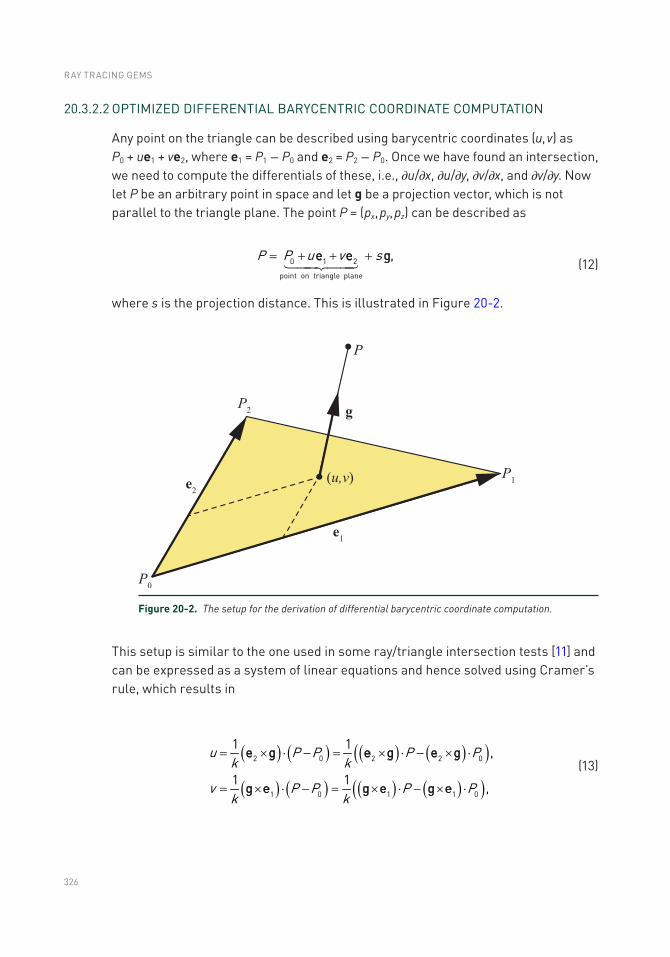
326
20.3.2.2 OPTIMIZED DIFFERENTIAL BARYCENTRIC COORDINATE COMPUTATION
Any point on the triangle can be described using barycentric coordinates (u, v) as P0 + ue1 + ve2, where e1 = P1 − P0 and e2 = P2 − P0. Once we have found an intersection, we need to compute the differentials of these, i.e., ∂u/∂x, ∂u/∂y, ∂v/∂x, and ∂v/∂y. Now let P be an arbitrary point in space and let g be a projection vector, which is not parallel to the triangle plane. The point P = (px, py, pz) can be described as
P P u v s= + + +e e g0 1 2
point on triangle plane
, (12)
where s is the projection distance. This is illustrated in Figure 20-2.
Figure 20-2. The setup for the derivation of differential barycentric coordinate computation.
This setup is similar to the one used in some ray/triangle intersection tests [11] and can be expressed as a system of linear equations and hence solved using Cramer’s rule, which results in
( ) ( ) ( ) ( )( )
( ) ( ) ( ) ( )( )
u P P P Pk k
v P P P Pk k
2 0 2 2 0
1 0 1 1 0
1 1 ,
1 1 ,
= ´ × - = ´ × - ´ ×
= ´ × - = ´ × - ´ ×
e g e g e g
g e g e g e
(13)
RAY TRACING GEMS
327
where k = (e1 × e2) ⋅ g. From these expressions, we can see that
( ) ( )u vP k P k2 1
1 1and .¶ ¶= ´ = ´
¶ ¶e g g e (14)
These expressions will be useful later on in the derivation. Next, assume that a point of intersection is computed as P = O + td (note that the ray direction vector d needs not be normalized), which means that we can express ∂P/∂x as
( ),
O tP O t ttx x x x x x
¶ +¶ ¶ ¶ ¶ ¶= = + + = +
¶ ¶ ¶ ¶ ¶ 
d d d q d (15)
where q = ∂O/∂x + t(∂ d/∂x). The same is done for ∂P/∂y, where we instead use r = ∂O/∂y + t(∂ d/∂y). We use the results from Equations 14 and 15 together with the chain rule to obtain
( )2
dot product
1 .yx z
x y z
pp pu u u u u P tx p x p x p x P x k x
¶¶ ¶¶ ¶ ¶ ¶ ¶ ¶ æ ¶ ö= + + = × = ´ × +ç ÷¶ ¶ ¶ ¶ ¶ ¶ ¶ ¶ ¶ ¶è ø
e g q d
(16)
Next, we choose g = d and simplify the previous expression to
( ) ( )u tx k x k2 2
1 1 ,¶ æ ¶ ö= ´ × + = ´ ×ç ÷¶ ¶è ø
e d q d e d q (17)
since (e2 × d) ⋅ d = 0. Now, the expressions for which we sought can be summarized as
u u
v v
u ux k y kv vx k y k
1 1and ,
1 1and ,
¶ ¶= × = ×
¶ ¶¶ 
= × = ׶ 
c q c r
c q c r
(18)
where
( )
u vO Ot tx x y y
k
2 1
1 2
, , , ,
and .
¶ ¶ ¶ ¶= ´ = ´ = + = +
¶ ¶ ¶ 
= ´ ×
d dc e d c d e q r
e e d (19)
TEXTURE LEVEL OF DETAIL STRATEGIES FOR REAL-TIME RAY TRACING
328
Note that q and r are evaluated using the ray differential representation in Equation 7 along with t, which is the distance to the intersection point. In addition, since w = 1 − u − v, we have
w u vx x x
,¶ ¶ ¶= - -
¶ ¶ ¶ (20)
and similarly for ∂w/∂y.
Once the differentials of (u, v) have been computed, they can be used to compute the corresponding texture-space differentials, which can be used in Equation 2, as
x x y y
x x y y
s u v t u vw g g h g gx x x x x xs u v t u vw g g h g gy y y y y y
1 2 1 2
1 2 1 2
, ,
, ,
¶ æ ¶ ¶ ö ¶ æ ¶ ¶ ö= + = +ç ÷ ç ÷¶ ¶ ¶ ¶ ¶ ¶è ø è ø
æ ö æ ö¶ ¶ ¶ ¶ ¶ ¶= + = +ç ÷ ç ÷¶ ¶ ¶ ¶ ¶ ¶è ø è ø
(21)
where w × h is the texture resolution and g1 = (g1x, g1y) = T1 − T0 and g2 = (g2x, g2y) = T2 − T0 are the differences of texture coordinates between neighboring vertices. Similarly, differentials for the ray origin O′ of a subsequent reflection/refraction ray can be computed as
( ) ( ) ( )
O u vx,y x,y x, y1 2.¶ ¶ ¶¢
= +¶ ¶ 
e e (22)
We have seen slightly better performance using this method compared to the traditional implementation following Igehy’s work [9].
20.3.3 RAY DIFFERENTIALS WITH THE G-BUFFER
For real-time ray tracing, it is not uncommon to render the eye rays using rasterization into a G-buffer. When combining ray differentials [9] with a G-buffer, the ray differential for the eye rays can be created as usual, but the interaction at the first hit must use the content from the G-buffer, since the original geometry is not available at that time. Here, we present one method using the G-buffer, which we assume has been created with normals n and with distances t from the camera to the first hit point (or alternatively the world-space position). We describe how the ray differential is set up when shooting the first reflection ray from the position in the G-buffer.
RAY TRACING GEMS
329
The idea of this method is simply to access the G-buffer to the right and above the current pixel and create a ray differential from these values. The normals and the distances t, for the current pixel (x, y) and for the neighbors (x + 1, y) and (x, y + 1), are read out from the G-buffer. Let us denote these by 0:0n for the current pixel,
1:0ˆ+n for the pixel to the right, and 0: 1ˆ +n for the pixel above, and similarly for other
variables. The eye ray directions e for these neighbors are computed next. At this point, we can compute the ray differential of the ray origin at the first hit as
O t tx 1:0 1:0 0:0 0:0ˆ ,ˆ+ +
¶= -
¶e e (23)
and similarly for ∂O/∂y. The ray differential direction is computed as
( ) ( ), ,x 1:0 1:0 0:0 0:0
ˆˆ ˆ ˆ ˆ ,+ +
¶= -
¶d r e n r e n (24)
where r is the shader function reflect(). Similar computations are
done for /ˆ y¶ ¶d . We now have all components of the ray differential,
O x, O y , x, yˆ ˆ/ / / /¶ ¶ ¶ ¶ ¶ ¶ ¶ ¶d d , which means that ray tracing with ray
differentials can commence from the first hit.
The method above is fast, but sometimes you hit different surfaces when comparing to the pixel to the right and above. A simple improvement is to test if t+1:0 − t0:0 > ε, where ε is a small number, and, if so, access the G-buffer at −1:0 instead and use the one with the smallest difference in t. The same approach is used for the y-direction. This method is a bit slower but gives substantially better results along depth discontinuities.
20.3.4 RAY CONES
One method for computing texture level of detail is based on tracing cones. This is quite similar to the method proposed by Amanatides [1], except that we use the method only for texture LOD and we derive the details on how to implement this, which are absent in previous work. The core idea is illustrated in Figure 20-3. When the texture LOD λ has been computed for a pixel, the texture sampler in the GPU is used to perform trilinear mipmapping [17].
TEXTURE LEVEL OF DETAIL STRATEGIES FOR REAL-TIME RAY TRACING
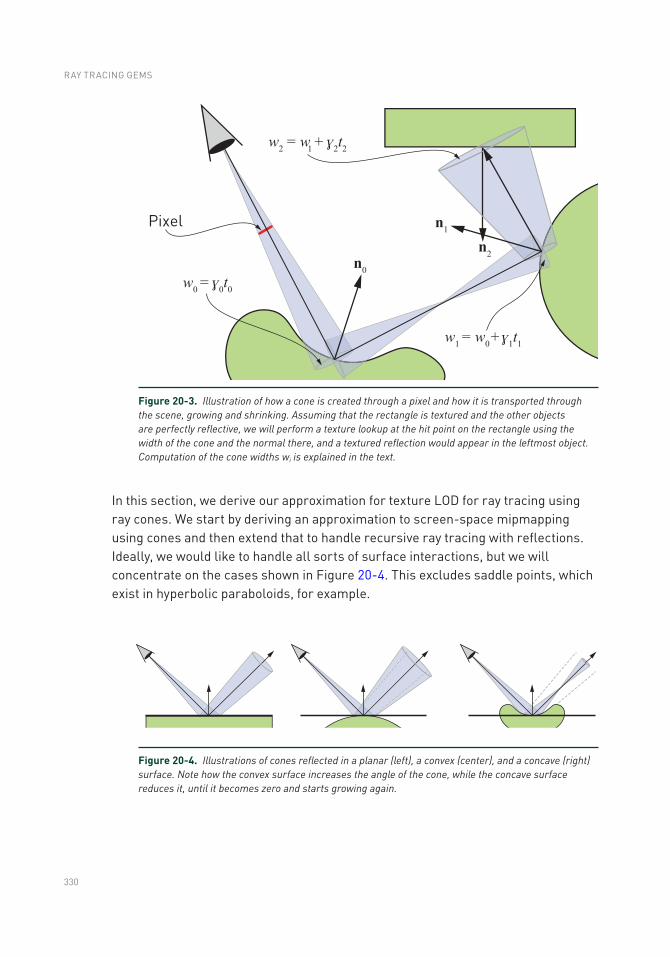
330
In this section, we derive our approximation for texture LOD for ray tracing using ray cones. We start by deriving an approximation to screen-space mipmapping using cones and then extend that to handle recursive ray tracing with reflections. Ideally, we would like to handle all sorts of surface interactions, but we will concentrate on the cases shown in Figure 20-4. This excludes saddle points, which exist in hyperbolic paraboloids, for example.
Figure 20-3. Illustration of how a cone is created through a pixel and how it is transported through the scene, growing and shrinking. Assuming that the rectangle is textured and the other objects are perfectly reflective, we will perform a texture lookup at the hit point on the rectangle using the width of the cone and the normal there, and a textured reflection would appear in the leftmost object. Computation of the cone widths wi is explained in the text.
Figure 20-4. Illustrations of cones reflected in a planar (left), a convex (center), and a concave (right) surface. Note how the convex surface increases the angle of the cone, while the concave surface reduces it, until it becomes zero and starts growing again.
RAY TRACING GEMS
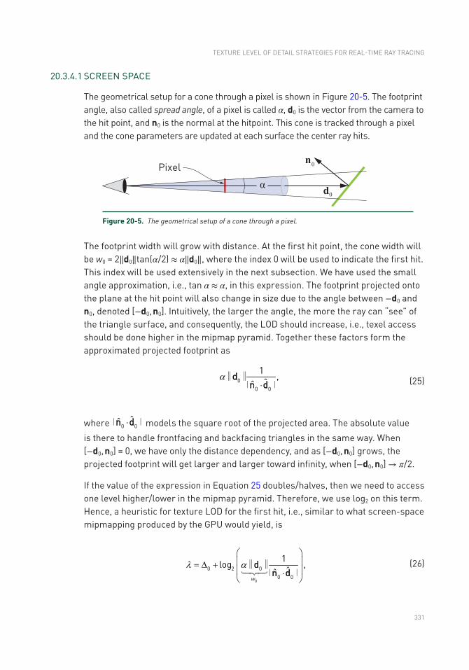
331
20.3.4.1 SCREEN SPACE
The geometrical setup for a cone through a pixel is shown in Figure 20-5. The footprint angle, also called spread angle, of a pixel is called α, d0 is the vector from the camera to the hit point, and n0 is the normal at the hitpoint. This cone is tracked through a pixel and the cone parameters are updated at each surface the center ray hits.
The footprint width will grow with distance. At the first hit point, the cone width will be w0 = 2‖d0‖tan(α/2) ≈ α‖d0‖, where the index 0 will be used to indicate the first hit. This index will be used extensively in the next subsection. We have used the small angle approximation, i.e., tan α ≈ α, in this expression. The footprint projected onto the plane at the hit point will also change in size due to the angle between −d0 and n0, denoted [−d0, n0]. Intuitively, the larger the angle, the more the ray can “see” of the triangle surface, and consequently, the LOD should increase, i.e., texel access should be done higher in the mipmap pyramid. Together these factors form the approximated projected footprint as
00 0
1 ,ˆˆ
a×
dn d
‖ ‖∣ ∣ (25)
where 0 0ˆˆ ×n d∣ ∣ models the square root of the projected area. The absolute value
is there to handle frontfacing and backfacing triangles in the same way. When [−d0, n0] = 0, we have only the distance dependency, and as [−d0, n0] grows, the projected footprint will get larger and larger toward infinity, when [−d0, n0] → π/2.
If the value of the expression in Equation 25 doubles/halves, then we need to access one level higher/lower in the mipmap pyramid. Therefore, we use log2 on this term. Hence, a heuristic for texture LOD for the first hit, i.e., similar to what screen-space mipmapping produced by the GPU would yield, is
w
l aæ öç ÷= D +ç ÷×è ø
dn d
0
0 2 00 0
1ˆˆ
log ,‖ ‖∣ ∣
(26)
Figure 20-5. The geometrical setup of a cone through a pixel.
TEXTURE LEVEL OF DETAIL STRATEGIES FOR REAL-TIME RAY TRACING
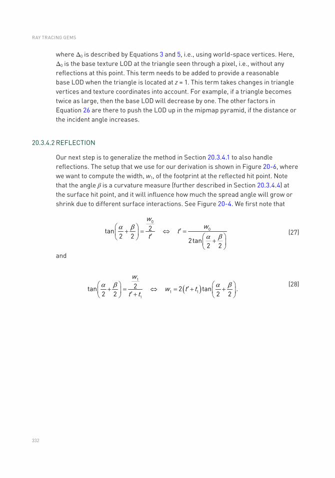
332
where Δ0 is described by Equations 3 and 5, i.e., using world-space vertices. Here, Δ0 is the base texture LOD at the triangle seen through a pixel, i.e., without any reflections at this point. This term needs to be added to provide a reasonable base LOD when the triangle is located at z = 1. This term takes changes in triangle vertices and texture coordinates into account. For example, if a triangle becomes twice as large, then the base LOD will decrease by one. The other factors in Equation 26 are there to push the LOD up in the mipmap pyramid, if the distance or the incident angle increases.
20.3.4.2 REFLECTION
Our next step is to generalize the method in Section 20.3.4.1 to also handle reflections. The setup that we use for our derivation is shown in Figure 20-6, where we want to compute the width, w1, of the footprint at the reflected hit point. Note that the angle β is a curvature measure (further described in Section 20.3.4.4) at the surface hit point, and it will influence how much the spread angle will grow or shrink due to different surface interactions. See Figure 20-4. We first note that
ww
tt
0
02tan2 2
2tan2 2
a ba b
æ ö+ = Û =ç ÷ æ öè ø +
¢çè
¢
÷ø
(27)
and
( )w
w t tt t
1
1 11
2tan 2 tan .2 2 2 2a b a b¢æ ö æ ö+ = Û = + +ç ÷ ç¢ ÷+è ø è ø
(28)
RAY TRACING GEMS
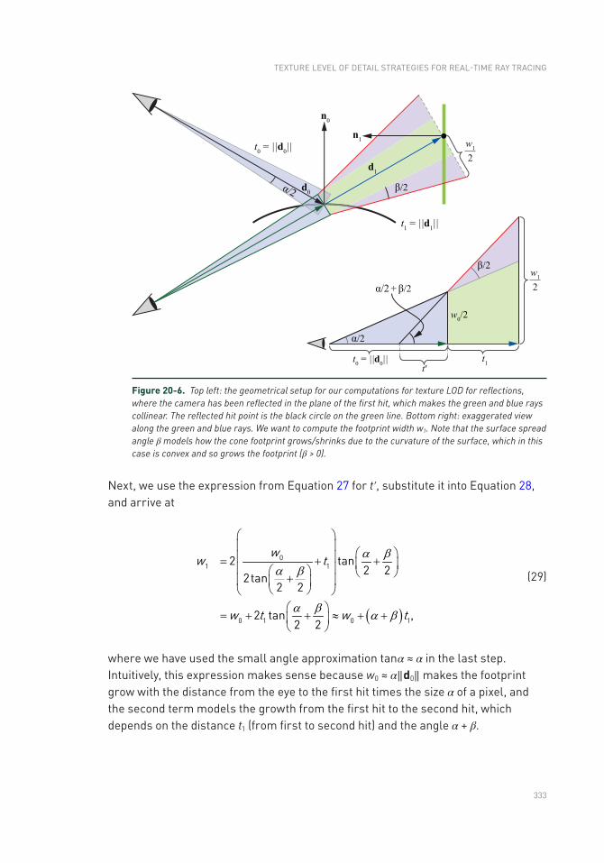
333
Next, we use the expression from Equation 27 for t′, substitute it into Equation 28, and arrive at
( )
ww t
w t w t
01 1
0 1 0 1
2 tan2 2
2tan2 2
2 tan ,2 2
a ba b
a b a b
æ öç ÷ æ öç ÷= + +ç ÷ç ÷æ ö è ø+ç ÷ç ÷
è øè øæ ö
= + + » + +ç ÷è ø
(29)
where we have used the small angle approximation tanα ≈ α in the last step. Intuitively, this expression makes sense because w0 ≈ α‖ d0‖ makes the footprint grow with the distance from the eye to the first hit times the size α of a pixel, and the second term models the growth from the first hit to the second hit, which depends on the distance t1 (from first to second hit) and the angle α + β.
Figure 20-6. Top left: the geometrical setup for our computations for texture LOD for reflections, where the camera has been reflected in the plane of the first hit, which makes the green and blue rays collinear. The reflected hit point is the black circle on the green line. Bottom right: exaggerated view along the green and blue rays. We want to compute the footprint width w1. Note that the surface spread angle β models how the cone footprint grows/shrinks due to the curvature of the surface, which in this case is convex and so grows the footprint (β > 0).
TEXTURE LEVEL OF DETAIL STRATEGIES FOR REAL-TIME RAY TRACING
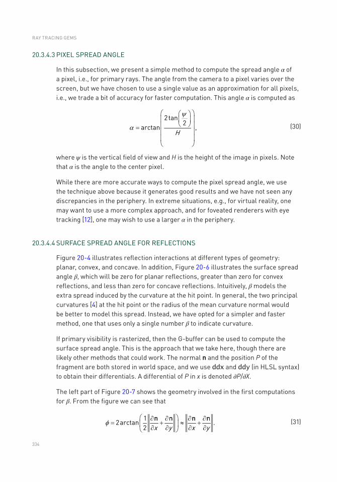
334
20.3.4.3 PIXEL SPREAD ANGLE
In this subsection, we present a simple method to compute the spread angle α of a pixel, i.e., for primary rays. The angle from the camera to a pixel varies over the screen, but we have chosen to use a single value as an approximation for all pixels, i.e., we trade a bit of accuracy for faster computation. This angle α is computed as
H
2tan2
arctan ,
y
a
æ öæ öç ÷ç ÷
è øç ÷=ç ÷ç ÷è ø
(30)
where ψ is the vertical field of view and H is the height of the image in pixels. Note that α is the angle to the center pixel.
While there are more accurate ways to compute the pixel spread angle, we use the technique above because it generates good results and we have not seen any discrepancies in the periphery. In extreme situations, e.g., for virtual reality, one may want to use a more complex approach, and for foveated renderers with eye tracking [12], one may wish to use a larger α in the periphery.
20.3.4.4 SURFACE SPREAD ANGLE FOR REFLECTIONS
Figure 20-4 illustrates reflection interactions at different types of geometry: planar, convex, and concave. In addition, Figure 20-6 illustrates the surface spread angle β, which will be zero for planar reflections, greater than zero for convex reflections, and less than zero for concave reflections. Intuitively, β models the extra spread induced by the curvature at the hit point. In general, the two principal curvatures [4] at the hit point or the radius of the mean curvature normal would be better to model this spread. Instead, we have opted for a simpler and faster method, one that uses only a single number β to indicate curvature.
If primary visibility is rasterized, then the G-buffer can be used to compute the surface spread angle. This is the approach that we take here, though there are likely other methods that could work. The normal n and the position P of the fragment are both stored in world space, and we use ddx and ddy (in HLSL syntax) to obtain their differentials. A differential of P in x is denoted ∂P/∂X.
The left part of Figure 20-7 shows the geometry involved in the first computations for β. From the figure we can see that
x y x y
12arctan .2
fæ ö¶ ¶ ¶ 
= + » +ç ÷¶ ¶ ¶ ¶è ø
n n n n (31)
RAY TRACING GEMS
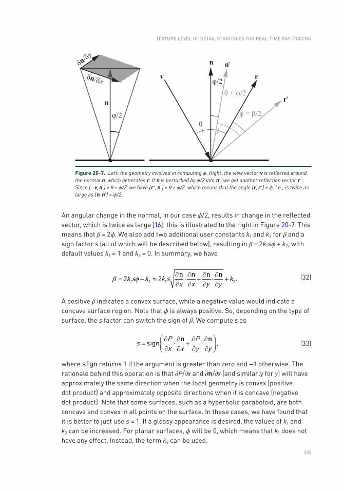
335
An angular change in the normal, in our case ϕ/2, results in change in the reflected vector, which is twice as large [16]; this is illustrated to the right in Figure 20-7. This means that β = 2ϕ. We also add two additional user constants k1 and k2 for β and a sign factor s (all of which will be described below), resulting in β = 2k1sϕ + k2, with default values k1 = 1 and k2 = 0. In summary, we have
k s k k s kx x y y1 2 1 22 2 .b f ¶ ¶ ¶ 
= + » × + × +¶ ¶ ¶ 
n n n n (32)
A positive β indicates a convex surface, while a negative value would indicate a concave surface region. Note that ϕ is always positive. So, depending on the type of surface, the s factor can switch the sign of β. We compute s as
P Psx x y y
sign ,æ ö¶ ¶ ¶ 
= × + ×ç ÷¶ ¶ ¶ ¶è ø
n n (33)
where sign returns 1 if the argument is greater than zero and −1 otherwise. The rationale behind this operation is that ∂P/∂x and ∂n/∂x (and similarly for y) will have approximately the same direction when the local geometry is convex (positive dot product) and approximately opposite directions when it is concave (negative dot product). Note that some surfaces, such as a hyperbolic paraboloid, are both concave and convex in all points on the surface. In these cases, we have found that it is better to just use s = 1. If a glossy appearance is desired, the values of k1 and k2 can be increased. For planar surfaces, ϕ will be 0, which means that k1 does not have any effect. Instead, the term k2 can be used.
Figure 20-7. Left: the geometry involved in computing ϕ. Right: the view vector v is reflected around the normal n, which generates r. If n is perturbed by ϕ/2 into n′, we get another reflection vector r ′. Since [−v, n′] = θ + ϕ/2, we have [r ′, n′] = θ + ϕ/2, which means that the angle [r, r ′] = ϕ, i.e., is twice as large as [n, n′] = ϕ/2.
TEXTURE LEVEL OF DETAIL STRATEGIES FOR REAL-TIME RAY TRACING
336
20.3.4.5 GENERALIZATION
Let i denote the enumerated hit point along a ray path, starting at 0. That is, the first hit is enumerated by 0, the second by 1, and so on. All our terms for texture LOD for the ith hit point are then put together as
i i i i i i ii i
w w2 2 2
Eqn.3 distance normal
1log log log ˆˆˆˆ
,læ öç ÷= D + × = D + - ×ç ÷×è ø
n dn d
(34)
and as can be seen, this is similar to Equation 26, with both a distance and a normal dependency. Refer to Figure 20-6 for the variables and recall that ni is the normal at the surface at the ith hit point and di is the vector to the ith hit point from the previous hit point. The base triangle LOD, Δi, now has a subscript i to indicate that it is the base LOD of the triangle at the ith hit point that should be used. Similar to before, id means a normalized direction of di. Note that we have added two absolute value functions in Equation 34. The absolute value for the distance term is there because β can be negative, e.g., for concave surface points (see the right part of Figure 20-4). The absolute value for the normal term is there to handle backfacing triangles in a consistent manner.
Note that w0 = αt0 = γ0t0 and w1 = αt0 + (α + β0)t1 = w0 + γ1t1, where we have introduced γ0 = α and γ1 = α + β0, and β0 is the surface spread angle at the first hit point. Hence, Equation 34 handles recursion, which we describe with pseudocode in Section 20.6, and in general it holds that
i i i iw w t1 ,g-= + (35)
where γi = γi − 1 + βi − 1. This is illustrated in Figure 20-3.
20.4 IMPLEMENTATION
We have implemented the ray cones and ray differentials techniques on top of Falcor [2] with DirectX 12 and DXR. For the texture lookups in ray cones, we compute λi according to Equation 34 and 35 and feed it into the SampleLevel() function of the texture.
Since rasterization is highly optimized for rendering primary visibility, where all rays share a single origin, we always use a G-buffer pass for ray cones and for the ray differentials method in Section 20.3.3. When a G-buffer is used, ray tracing commences from the first hit described by the G-buffer. As a consequence, texturing is done using the GPU’s texturing units for the first hits and so, using the methods in this chapter, λ is computed only after that. For ray cones, βi is computed
RAY TRACING GEMS
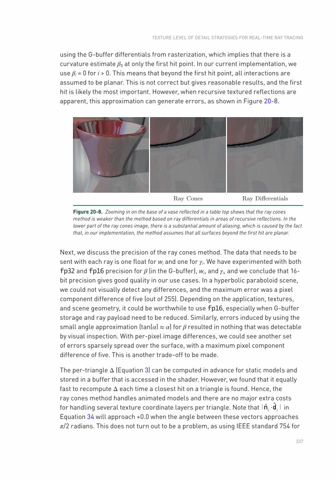
337
using the G-buffer differentials from rasterization, which implies that there is a curvature estimate β0 at only the first hit point. In our current implementation, we use βi = 0 for i > 0. This means that beyond the first hit point, all interactions are assumed to be planar. This is not correct but gives reasonable results, and the first hit is likely the most important. However, when recursive textured reflections are apparent, this approximation can generate errors, as shown in Figure 20-8.
Next, we discuss the precision of the ray cones method. The data that needs to be sent with each ray is one float for wi and one for γi. We have experimented with both fp32 and fp16 precision for β (in the G-buffer), wi, and γi, and we conclude that 16- bit precision gives good quality in our use cases. In a hyperbolic paraboloid scene, we could not visually detect any differences, and the maximum error was a pixel component difference of five (out of 255). Depending on the application, textures, and scene geometry, it could be worthwhile to use fp16, especially when G-buffer storage and ray payload need to be reduced. Similarly, errors induced by using the small angle approximation (tan(α) ≈ α) for β resulted in nothing that was detectable by visual inspection. With per-pixel image differences, we could see another set of errors sparsely spread over the surface, with a maximum pixel component difference of five. This is another trade-off to be made.
The per-triangle Δ (Equation 3) can be computed in advance for static models and stored in a buffer that is accessed in the shader. However, we found that it equally fast to recompute Δ each time a closest hit on a triangle is found. Hence, the ray cones method handles animated models and there are no major extra costs for handling several texture coordinate layers per triangle. Note that i i
ˆˆ ×n d∣ ∣ in Equation 34 will approach +0.0 when the angle between these vectors approaches π/2 radians. This does not turn out to be a problem, as using IEEE standard 754 for
Figure 20-8. Zooming in on the base of a vase reflected in a table top shows that the ray cones method is weaker than the method based on ray differentials in areas of recursive reflections. In the lower part of the ray cones image, there is a substantial amount of aliasing, which is caused by the fact that, in our implementation, the method assumes that all surfaces beyond the first hit are planar.
TEXTURE LEVEL OF DETAIL STRATEGIES FOR REAL-TIME RAY TRACING
338
floating-point mathematics, we have log2 (+0.0) = –inf, which makes λ = inf. This in turn will force the trilinear lookup to access the top level of the mipmap hierarchy, which is expected when the angle is π/2 radians.
Our ray differentials implementation follows the description of Igehy [9] fairly well. However, we use the λ computation in Equations 1 and 2, unless otherwise mentioned, and the methods in Sections 20.3.2.1 and 20.3.2.2. For ray differentials, each ray needs 12 floats of storage, which is rather substantial.
20.5 COMPARISON AND RESULTS
The methods that we use in this section are:
> Groundtruth: a ground-truth rendering (ray traced with 1,024 samples per pixel).
> Mip0: bilinearly filtered mip level 0.
> RayCones: ray cones method (Section 20.3.4).
> RayDiffs GB: ray differentials with the G-buffer (Section 20.3.3).
> RayDiffs RT: our implementation of ray differentials with ray tracing [9].
> RayDiffs PBRT: ray differentials implementation in the pbrt renderer [14].
Note that Mip0, RayCones, and RayDiffs GB always use a G-buffer for primary visibility, while RayDiffs RT and RayDiffs PBRT use ray tracing. For all our performance results, an NVIDIA RTX 2080 Ti (Turing) was used with driver 416.16.
To verify that our implementation of ray differentials [9] is correct, we compared it to the implementation in the pbrt renderer [14]. To visualize the resulting mip level of a filtered textured lookup, we use a specialized rainbow texture, shown in Figure 20-9. Each mip level is set to a single color. We rendered a reflective hyperbolic paraboloid in a diffuse room in Figure 20-10. This means that the room only shows the mip level as seen from the eye, while the hyperbolic paraboloid shows the mip level of the reflection, which has some consequences discussed in the caption of Figure 20-10. It is noteworthy that one can see the triangular structure of the hyperbolic paraboloid surface in these images. The reason for this is that the differentials of barycentric coordinates are not continuous across shared triangle edges. This is also true for rasterization, which shows similar structures. As a consequence, this discontinuity generates noise in the recursive reflections, but it does not show up visually in the rendered images in our video.
RAY TRACING GEMS
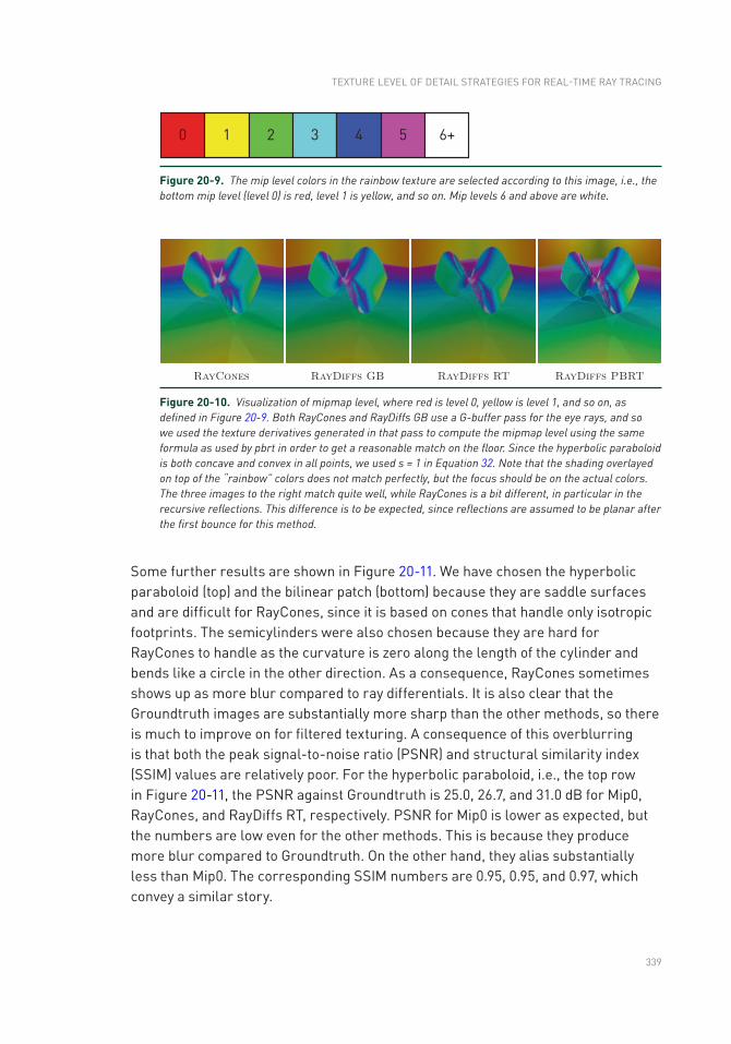
339
Some further results are shown in Figure 20-11. We have chosen the hyperbolic paraboloid (top) and the bilinear patch (bottom) because they are saddle surfaces and are difficult for RayCones, since it is based on cones that handle only isotropic footprints. The semicylinders were also chosen because they are hard for RayCones to handle as the curvature is zero along the length of the cylinder and bends like a circle in the other direction. As a consequence, RayCones sometimes shows up as more blur compared to ray differentials. It is also clear that the Groundtruth images are substantially more sharp than the other methods, so there is much to improve on for filtered texturing. A consequence of this overblurring is that both the peak signal-to-noise ratio (PSNR) and structural similarity index (SSIM) values are relatively poor. For the hyperbolic paraboloid, i.e., the top row in Figure 20-11, the PSNR against Groundtruth is 25.0, 26.7, and 31.0 dB for Mip0, RayCones, and RayDiffs RT, respectively. PSNR for Mip0 is lower as expected, but the numbers are low even for the other methods. This is because they produce more blur compared to Groundtruth. On the other hand, they alias substantially less than Mip0. The corresponding SSIM numbers are 0.95, 0.95, and 0.97, which convey a similar story.
Figure 20-9. The mip level colors in the rainbow texture are selected according to this image, i.e., the bottom mip level (level 0) is red, level 1 is yellow, and so on. Mip levels 6 and above are white.
Figure 20-10. Visualization of mipmap level, where red is level 0, yellow is level 1, and so on, as defined in Figure 20-9. Both RayCones and RayDiffs GB use a G-buffer pass for the eye rays, and so we used the texture derivatives generated in that pass to compute the mipmap level using the same formula as used by pbrt in order to get a reasonable match on the floor. Since the hyperbolic paraboloid is both concave and convex in all points, we used s = 1 in Equation 32. Note that the shading overlayed on top of the “rainbow” colors does not match perfectly, but the focus should be on the actual colors. The three images to the right match quite well, while RayCones is a bit different, in particular in the recursive reflections. This difference is to be expected, since reflections are assumed to be planar after the first bounce for this method.
TEXTURE LEVEL OF DETAIL STRATEGIES FOR REAL-TIME RAY TRACING
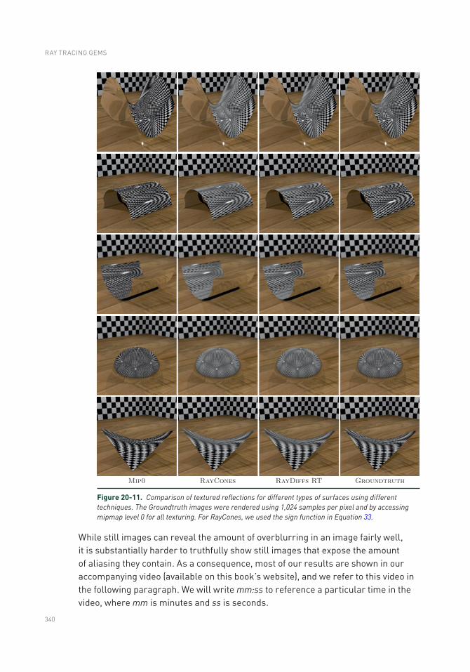
340
While still images can reveal the amount of overblurring in an image fairly well, it is substantially harder to truthfully show still images that expose the amount of aliasing they contain. As a consequence, most of our results are shown in our accompanying video (available on this book’s website), and we refer to this video in the following paragraph. We will write mm:ss to reference a particular time in the video, where mm is minutes and ss is seconds.
Figure 20-11. Comparison of textured reflections for different types of surfaces using different techniques. The Groundtruth images were rendered using 1,024 samples per pixel and by accessing mipmap level 0 for all texturing. For RayCones, we used the sign function in Equation 33.
RAY TRACING GEMS
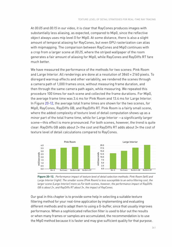
341
At 00:05 and 00:15 in our video, it is clear that RayCones produces images with substantially less aliasing, as expected, compared to Mip0, since the reflective object always uses mip level 0 for Mip0. At some distance, there is also a slight amount of temporal aliasing for RayCones, but even GPU rasterization can alias with mipmapping. The comparison between RayCones and Mip0 continues with a crop from a larger scene at 00:25, where the striped wallpaper of the room generates a fair amount of aliasing for Mip0, while RayCones and RayDiffs RT fare much better.
We have measured the performance of the methods for two scenes: Pink Room and Large Interior. All renderings are done at a resolution of 3840 × 2160 pixels. To disregard warmup effects and other variability, we rendered the scenes through a camera path of 1,000 frames once, without measuring frame duration, and then through the same camera path again, while measuring. We repeated this procedure 100 times for each scene and collected the frame durations. For Mip0, the average frame time was 3.4 ms for Pink Room and 13.4 ms for Large Interior. In Figure 20-12, the average total frame times are shown for the two scenes, for Mip0, RayCones, RayDiffs GB, and RayDiffs RT. Pink Room is a fairly small scene, where the added complexity of texture level of detail computation shows up as a minor part of the total frame time, while for Large Interior —a significantly larger scene—this effect is more pronounced. For both scenes, however, the trend is quite clear: RayDiffs GB adds about 2× the cost and RayDiffs RT adds about 3× the cost of texture level of detail calculations compared to RayCones.
Our goal in this chapter is to provide some help in selecting a suitable texture filtering method for your real-time application by implementing and evaluating different methods and to adapt them to using a G-buffer, since that usually improves performance. When a sophisticated reflection filter is used to blur out the results or when many frames or samples are accumulated, the recommendation is to use the Mip0 method because it is faster and may give sufficient quality for that purpose.
MIP-O RAYCONES RAYDIFFS GB RAYDIFFS RT
Pink Room
0.00.51.01.52.0
mill
isec
onds 2.5
3.03.54.0
RAYDIFFS GB RAYDIFFS RTMIP-O RAYCONES
Large Interior
0.02.55.07.5
10.0
mill
isec
onds 12.5
15.017.520.0
Figure 20-12. Performance impact of texture level of detail selection methods: Pink Room (left) and Large Interior (right). The smaller scene (Pink Room) is less susceptible to an extra filtering cost, the larger scene (Large Interior) more so.For both scenes, however, the performance impact of RayDiffs GB is about 2×, and RayDiffs RT about 3×, the impact of RayCones.
TEXTURE LEVEL OF DETAIL STRATEGIES FOR REAL-TIME RAY TRACING
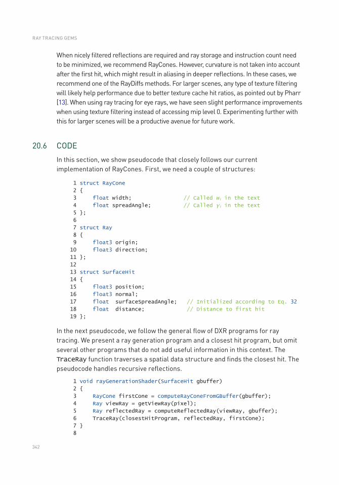
342
When nicely filtered reflections are required and ray storage and instruction count need to be minimized, we recommend RayCones. However, curvature is not taken into account after the first hit, which might result in aliasing in deeper reflections. In these cases, we recommend one of the RayDiffs methods. For larger scenes, any type of texture filtering will likely help performance due to better texture cache hit ratios, as pointed out by Pharr [13]. When using ray tracing for eye rays, we have seen slight performance improvements when using texture filtering instead of accessing mip level 0. Experimenting further with this for larger scenes will be a productive avenue for future work.
20.6 CODE
In this section, we show pseudocode that closely follows our current implementation of RayCones. First, we need a couple of structures:
1 struct RayCone
2
3 float width; // Called wi in the text
4 float spreadAngle; // Called γi in the text
5 ;
6
7 struct Ray
8
9 float3 origin;
10 float3 direction;
11 ;
12
13 struct SurfaceHit
14
15 float3 position;
16 float3 normal;
17 float surfaceSpreadAngle; // Initialized according to Eq. 32
18 float distance; // Distance to first hit
19 ;
In the next pseudocode, we follow the general flow of DXR programs for ray tracing. We present a ray generation program and a closest hit program, but omit several other programs that do not add useful information in this context. The TraceRay function traverses a spatial data structure and finds the closest hit. The pseudocode handles recursive reflections.
1 void rayGenerationShader(SurfaceHit gbuffer)
2
3 RayCone firstCone = computeRayConeFromGBuffer(gbuffer);
4 Ray viewRay = getViewRay(pixel);
5 Ray reflectedRay = computeReflectedRay(viewRay, gbuffer);
6 TraceRay(closestHitProgram, reflectedRay, firstCone);
7
8
RAY TRACING GEMS
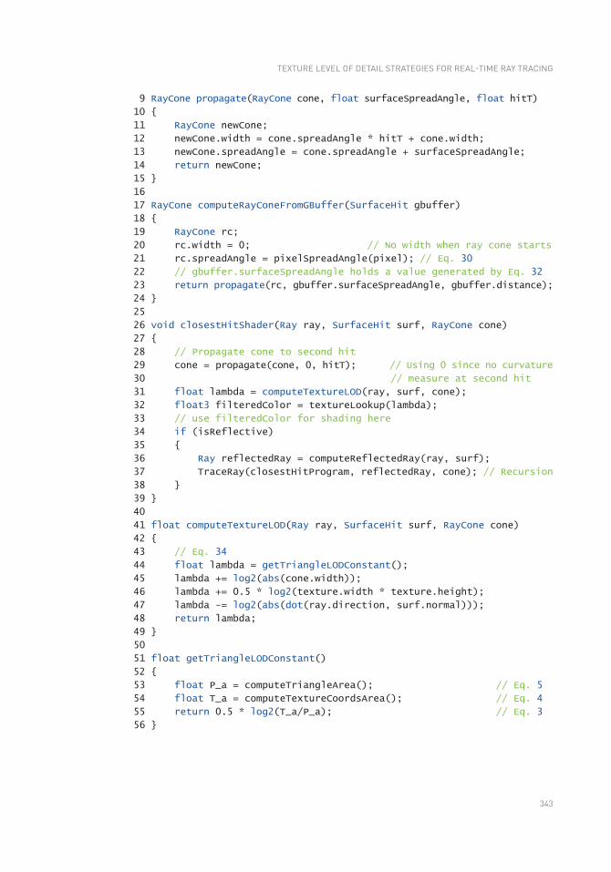
343
9 RayCone propagate(RayCone cone, float surfaceSpreadAngle, float hitT)
10
11 RayCone newCone;
12 newCone.width = cone.spreadAngle * hitT + cone.width;
13 newCone.spreadAngle = cone.spreadAngle + surfaceSpreadAngle;
14 return newCone;
15
16
17 RayCone computeRayConeFromGBuffer(SurfaceHit gbuffer)
18
19 RayCone rc;
20 rc.width = 0; // No width when ray cone starts
21 rc.spreadAngle = pixelSpreadAngle(pixel); // Eq. 30
22 // gbuffer.surfaceSpreadAngle holds a value generated by Eq. 32
23 return propagate(rc, gbuffer.surfaceSpreadAngle, gbuffer.distance);
24
25
26 void closestHitShader(Ray ray, SurfaceHit surf, RayCone cone)
27
28 // Propagate cone to second hit
29 cone = propagate(cone, 0, hitT); // Using 0 since no curvature
30 // measure at second hit
31 float lambda = computeTextureLOD(ray, surf, cone);
32 float3 filteredColor = textureLookup(lambda);
33 // use filteredColor for shading here
34 if (isReflective)
35
36 Ray reflectedRay = computeReflectedRay(ray, surf);
37 TraceRay(closestHitProgram, reflectedRay, cone); // Recursion
38
39
40
41 float computeTextureLOD(Ray ray, SurfaceHit surf, RayCone cone)
42
43 // Eq. 34
44 float lambda = getTriangleLODConstant();
45 lambda += log2(abs(cone.width));
46 lambda += 0.5 * log2(texture.width * texture.height);
47 lambda -= log2(abs(dot(ray.direction, surf.normal)));
48 return lambda;
49
50
51 float getTriangleLODConstant()
52
53 float P_a = computeTriangleArea(); // Eq. 5
54 float T_a = computeTextureCoordsArea(); // Eq. 4
55 return 0.5 * log2(T_a/P_a); // Eq. 3
56
TEXTURE LEVEL OF DETAIL STRATEGIES FOR REAL-TIME RAY TRACING

344
ACKNOWLEDGMENTS
Thanks to Jacob Munkberg and Jon Hasselgren for brainstorming help and comments.
REFERENCES
[1] Amanatides, J. Ray Tracing with Cones. Computer Graphics (SIGGRAPH) 18, 3 (1984), 129–135.
[2] Benty, N., Yao, K.-H., Foley, T., Kaplanyan, A. S., Lavelle, C., Wyman, C., and Vijay, A. The Falcor Rendering Framework. https://github.com/NVIDIAGameWorks/Falcor, July 2017.
[3] Christensen, P., Fong, J., Shade, J., Wooten, W., Schubert, B., Kensler, A., Friedman, S., Kilpatrick, C., Ramshaw, C., Bannister, M., Rayner, B., Brouillat, J., and Liani, M. RenderMan: An Advanced Path-Tracing Architecture for Movie Rendering. ACM Transactions on Graphics 37, 3 (2018), 30:1–30:21.
[4] do Carmo, M. P. Differential Geometry of Curves and Surfaces. Prentice Hall Inc., 1976.
[5] Ewins, J. P., Waller, M. D., White, M., and Lister, P. F. MIP-Map Level Selection for Texture Mapping. IEEE Transactions on Visualization and Computer Graphics 4, 4 (1998), 317–329.
[6] Green, N., and Heckbert, P. S. Creating Raster Omnimax Images from Multiple Perspective Views Using the Elliptical Weighted Average Filter. IEEE Computer Graphics and Applications 6, 6 (1986), 21–27.
[7] Heckbert, P. S. Survey of Texture Mapping. IEEE Computer Graphics and Applications 6, 11 (1986), 56–67.
[8] Heckbert, P. S. Fundamentals of Texture Mapping and Image Warping. Master’s thesis, University of California, Berkeley, 1989.
[9] Igehy, H. Tracing Ray Differentials. In Proceedings of SIGGRAPH (1999), pp. 179–186.
[10] McCormack, J., Perry, R., Farkas, K. I., and Jouppi, N. P. Feline: Fast Elliptical Lines for Anisotropic Texture Mapping. In Proceedings of SIGGRAPH (1999), pp. 243–250.
[11] Möller, T., and Trumbore, B. Fast, Minimum Storage Ray-Triangle Intersection. Journal of Graphics Tools 2, 1 (1997), 21–28.
[12] Patney, A., Salvi, M., Kim, J., Kaplanyan, A., Wyman, C., Benty, N., Luebke, D., and Lefohn, A. Towards Foveated Rendering for Gaze-Tracked Virtual Reality. ACM Transactions on Graphics 35, 6 (2016), 179:1–179:12.
[13] Pharr, M. Swallowing the Elephant (Part 5). Matt Pharr’s blog, https://pharr.org/matt/blog/2018/07/16/moana-island-pbrt-5.html, July 16 2018.
RAY TRACING GEMS

345
[14] Pharr, M., Jakob, W., and Humphreys, G. Physically Based Rendering: From Theory to Implementation, third ed. Morgan Kaufmann, 2016.
[15] Segal, M., and Akeley, K. The OpenGL Graphics System: A Specification (Version 4.5). Khronos Group documentation, 2016.
[16] Voorhies, D., and Foran, J. Reflection Vector Shading Hardware. In Proceedings of SIGGRAPH (1994), pp. 163–166.
[17] Williams, L. Pyramidal Parametrics. Computer Graphics (SIGGRAPH) 17, 3 (1983), 1–11.
Open Access This chapter is licensed under the terms of the Creative Commons Attribution-NonCommercial-NoDerivatives 4.0 International License (http://creativecommons.org/licenses/by-nc-nd/4.0/), which permits any noncommercial use, sharing, distribution and
reproduction in any medium or format, as long as you give appropriate credit to the original author(s) and the source, provide a link to the Creative Commons license and indicate if you modified the licensed material. You do not have permission under this license to share adapted material derived from this chapter or parts of it.
The images or other third party material in this chapter are included in the chapter's Creative Commons license, unless indicated otherwise in a credit line to the material. If material is not included in the chapter's Creative Commons license and your intended use is not permitted by statutory regulation or exceeds the permitted use, you will need to obtain permission directly from the copyright holder.
TEXTURE LEVEL OF DETAIL STRATEGIES FOR REAL-TIME RAY TRACING
347© NVIDIA 2019 E. Haines, T. Akenine-Möller (eds.), Ray Tracing Gems, https://doi.org/10.1007/978-1-4842-4427-2_21
CHAPTER 21
Simple Environment Map Filtering Using Ray Cones and Ray DifferentialsTomas Akenine-Möller and Jim NilssonNVIDIA
ABSTRACT
We describe simple methods for how to filter environment maps using ray cones and ray differentials in a ray tracing engine.
21.1 INTRODUCTION
Environment maps (EMs) are commonly used in rendering as an inexpensive way of visually representing a scene far away. Another common usage is to let an EM represent the incoming illumination from a surrounding environment and use it to shade geometry [4]. Two common environment-mapping layouts are latitude-longitude maps [2] and cube maps [5].
Rasterization occurs in quads, i.e., 2 × 2 pixels at a time, which means that differentials can be estimated as horizontal and vertical pixel differences. These differentials can be used to compute a level of detail in order to perform a texture lookup using mipmapping. The concept of quads is not available in ray tracing, however. Instead, texture filtering is usually handled using ray differentials [6] or ray cones [1, 3]. These two methods are presented in Chapter 20. For ray differentials, Pharr et al. [7] used a forward differencing approximation to compute ray differentials in texture space for EMs. The major parts of the computations involved are three vector normalizations and six inverse trigonometric function calls.
Since the environment map is assumed to be positioned infinitely far away, environment mapping using rasterization depends on only the reflection vector, i.e., the directional component, and not on the position where the reflection vector was computed. For ray cones and ray differentials, there are also positional components of the ray representations. Similar to rasterization, however, these need not be used, as argued in Figure 21-1. In this chapter, we provide the formulas to compute EM filtering for both ray cones and ray differentials.
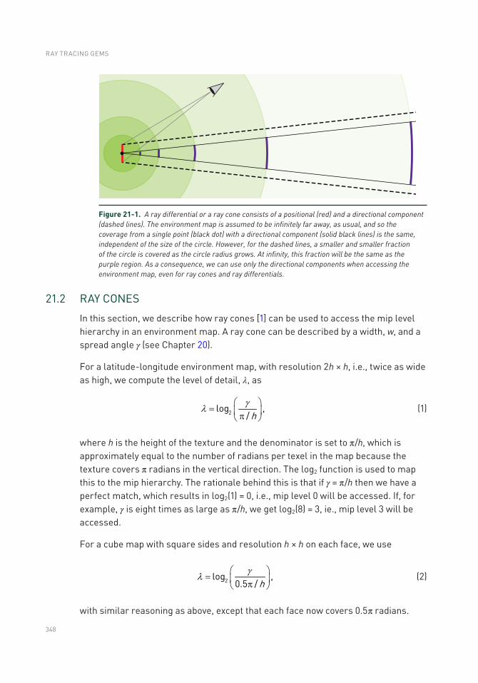
348
21.2 RAY CONES
In this section, we describe how ray cones [1] can be used to access the mip level hierarchy in an environment map. A ray cone can be described by a width, w, and a spread angle γ (see Chapter 20).
For a latitude-longitude environment map, with resolution 2h × h, i.e., twice as wide as high, we compute the level of detail, λ, as
h2log ,/gl æ ö
= ç ÷pè ø (1)
where h is the height of the texture and the denominator is set to π/h, which is approximately equal to the number of radians per texel in the map because the texture covers π radians in the vertical direction. The log2 function is used to map this to the mip hierarchy. The rationale behind this is that if γ = π/h then we have a perfect match, which results in log2(1) = 0, i.e., mip level 0 will be accessed. If, for example, γ is eight times as large as π/h, we get log2(8) = 3, ie., mip level 3 will be accessed.
For a cube map with square sides and resolution h × h on each face, we use
2log ,
0.5 / hgl æ ö
= ç ÷pè ø (2)
with similar reasoning as above, except that each face now covers 0.5π radians.
Figure 21-1. A ray differential or a ray cone consists of a positional (red) and a directional component (dashed lines). The environment map is assumed to be infinitely far away, as usual, and so the coverage from a single point (black dot) with a directional component (solid black lines) is the same, independent of the size of the circle. However, for the dashed lines, a smaller and smaller fraction of the circle is covered as the circle radius grows. At infinity, this fraction will be the same as the purple region. As a consequence, we can use only the directional components when accessing the environment map, even for ray cones and ray differentials.
RAY TRACING GEMS
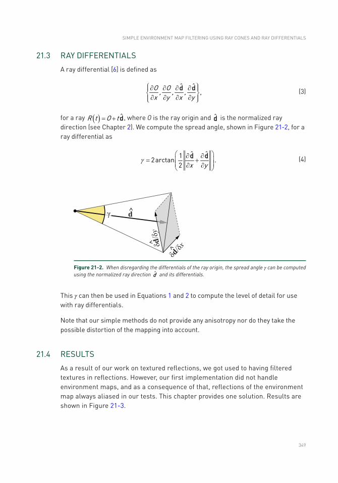
349
21.3 RAY DIFFERENTIALS
A ray differential [6] is defined as
ˆ ˆ,O O, , ,
x y x yì ü¶ ¶ ¶ ¶ï ïí ý¶ ¶ ¶ ¶ï ïî þ
d d
(3)
for a ray ( ) ˆR t O t= + d, where O is the ray origin and d is the normalized ray direction (see Chapter 2). We compute the spread angle, shown in Figure 21-2, for a ray differential as
12arctˆ
an .2
ˆ
x yg
æ ö¶ ¶= +ç ÷ç ÷¶ ¶è ø
d d
(4)
This γ can then be used in Equations 1 and 2 to compute the level of detail for use with ray differentials.
Note that our simple methods do not provide any anisotropy nor do they take the possible distortion of the mapping into account.
21.4 RESULTS
As a result of our work on textured reflections, we got used to having filtered textures in reflections. However, our first implementation did not handle environment maps, and as a consequence of that, reflections of the environment map always aliased in our tests. This chapter provides one solution. Results are shown in Figure 21-3.
Figure 21-2. When disregarding the differentials of the ray origin, the spread angle γ can be computed using the normalized ray direction d and its differentials.
SIMPLE ENVIRONMENT MAP FILTERINg USINg RAY CONES AND RAY DIFFERENTIALS
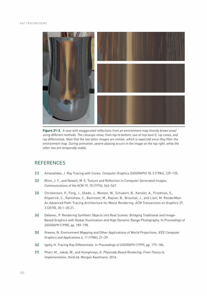
350
REFERENCES
[1] Amanatides, J. Ray Tracing with Cones. Computer Graphics (SIGGRAPH) 18, 3 (1984), 129–135.
[2] Blinn, J. F., and Newell, M. E. Texture and Reflection in Computer generated Images. Communications of the ACM 19, 10 (1976), 542–547.
[3] Christensen, P., Fong, J., Shade, J., Wooten, W., Schubert, B., Kensler, A., Friedman, S., Kilpatrick, C., Ramshaw, C., Bannister, M., Rayner, B., Brouillat, J., and Liani, M. RenderMan: An Advanced Path-Tracing Architecture for Movie Rendering. ACM Transactions on Graphics 37, 3 (2018), 30:1–30:21.
[4] Debevec, P. Rendering Synthetic Objects into Real Scenes: Bridging Traditional and Image-Based graphics with global Illumination and High Dynamic Range Photography. In Proceedings of SIGGRAPH (1998), pp. 189–198.
[5] greene, N. Environment Mapping and Other Applications of World Projections. IEEE Computer Graphics and Applications 6, 11 (1986), 21–29.
[6] Igehy, H. Tracing Ray Differentials. In Proceedings of SIGGRAPH (1999), pp. 179–186.
[7] Pharr, M., Jakob, W., and Humphreys, g. Physically Based Rendering: From Theory to Implementation, third ed. Morgan Kaufmann, 2016.
Figure 21-3. A vase with exaggerated reflections from an environment map (mostly brown area) using different methods. The closeups show, from top to bottom, use of mip level 0, ray cones, and ray differentials. Note that the two latter images are similar, which is expected since they filter the environment map. During animation, severe aliasing occurs in the image on the top right, while the other two are temporally stable.
RAY TRACING GEMS

351
Open Access This chapter is licensed under the terms of the Creative Commons Attribution-NonCommercial-NoDerivatives 4.0 International License (http://creativecommons.org/licenses/by-nc-nd/4.0/), which permits any noncommercial use, sharing, distribution and
reproduction in any medium or format, as long as you give appropriate credit to the original author(s) and the source, provide a link to the Creative Commons license and indicate if you modified the licensed material. You do not have permission under this license to share adapted material derived from this chapter or parts of it.
The images or other third party material in this chapter are included in the chapter's Creative Commons license, unless indicated otherwise in a credit line to the material. If material is not included in the chapter's Creative Commons license and your intended use is not permitted by statutory regulation or exceeds the permitted use, you will need to obtain permission directly from the copyright holder.
SIMPLE ENVIRONMENT MAP FILTERINg USINg RAY CONES AND RAY DIFFERENTIALS
353© NVIDIA 2019 E. Haines, T. Akenine-Möller (eds.), Ray Tracing Gems, https://doi.org/10.1007/978-1-4842-4427-2_22
CHAPTER 22
Improving Temporal Antialiasing with Adaptive Ray TracingAdam Marrs, Josef Spjut, Holger Gruen, Rahul Sathe, and Morgan McGuireNVIDIA
ABSTRACT
In this chapter, we discuss a pragmatic approach to real-time supersampling that extends commonly used temporal antialiasing techniques with adaptive ray tracing. The algorithm conforms to the constraints of a commercial game engine, removes blurring and ghosting artifacts associated with standard temporal antialiasing, and achieves quality approaching 16× supersampling of geometry, shading, and materials within the 16 ms frame budget required of most games.
22.1 INTRODUCTION
Aliasing of primary visible surfaces is one of the most fundamental and challenging limitations of computer graphics. Almost all rendering methods sample surfaces at points within pixels and thus produce errors when the points sampled are not representative of the pixel as a whole, that is, when primary surfaces are undersampled. This is true regardless of whether the points are tested by casting a ray or by the amortized ray casts of rasterization, and regardless of what shading algorithm is employed. Even “point-based” renderers [15] actually ray trace or splat points to the screen via rasterization. Analytic renderers such as perfect beam tracing in space and time could avoid the ray (under)sampling problem, but despite some analytic solutions for limited cases [1], point samples from ray or raster intersections remain the only fully developed approach for efficient rendering of complex geometry, materials, and shading.
Aliasing due to undersampling manifests as jagged edges, spatial noise, and flickering (temporal noise). Attempts to conceal these errors by wider and more sophisticated reconstruction filters in space (e.g., morphological antialiasing (MLAA) [22], fast approximate antialiasing (FXAA) [17]) and time (e.g., subpixel morphological antialiasing (SMAA) [12], temporal antialiasing (TAA) [13, 27]) convert those artifacts into blurring (in space) or ghosting (blurring in time). Under a fixed sample count per pixel across an image, the only true solution to aliasing is to increase the sample density and band-limit the signal being
354
sampled. Increasing density helps but does not solve the problem at rates affordable for real time: supersampling antialiasing (SSAA) incurs a cost linearly proportional to the number of samples while only increasing quality with the square root; multisampling (MSAA)—including coverage sampling (CSAA), surface based (SBAA) [24], and subpixel reconstruction (SRAA) [4]—samples geometry, materials, and shading at varying rates to heuristically reduce the cost but also lowers quality; and aggregation (decoupled coverage (DCAA) [25], aggregate G-buffer (AGAA) [7]) reduces cost even more aggressively but still limits quality at practical rates. For band-limiting the scene, material prefiltering by mipmapping and its variants [19], level of detail for geometry, and shader level of detail reduce the undersampling artifacts but introduce other nontrivial problems such as overblurring or popping (temporal and spatial discontinuities) while complicating rendering systems and failing to completely address the problem.
The standard in real-time rendering is to employ many of these strategies simultaneously, with a focus on leveraging temporal antialiasing. Despite succeeding in many cases, these game-specific solutions require significant engineering complexity and careful hand-tuning of scenes by artists [20, 21]. Since all these solutions depend on a fixed sampling count per pixel, an adversary can always place material, geometric, or shading features between samples to create unbounded error. More recently, Holländer et al. [10] aggressively identified pixels in need of antialiasing from coarse shading and high-resolution geometry passes and achieved nearly identical results to SSAA. Unfortunately, this rasterization-based approach requires processing all geometry at high resolutions even if only a few pixels are identified for antialiasing. Despite cutting the number of shading samples in half, the reduction in frame time is limited to 10%. Thus, we consider the aliasing challenge open for real-time rendering.
In this chapter, we describe a new pragmatic algorithm, Adaptive Temporal Antialiasing (ATAA), that attacks the aliasing problem by extending temporal antialiasing of rasterized images with adaptive ray traced supersampling. Offline ray tracing renderers have long employed highly adaptive sample counts to solve aliasing (e.g., Whitted’s original paper [26]), but until now hybrid ray and raster algorithms [2] have been impractical for real-time rendering due to the duplication of data structures between ray and raster APIs and architectures. The recent introduction of the DirectX Raytracing API (DXR) and the NVIDIA RTX platform enable full interoperability between data structures and shaders for both types of rendering on the GPU across the full game engine. Crucially, RTX substantially improves ray tracing performance by delivering hardware acceleration of the bounding volume hierarchy (BVH) traversal and triangle intersection tasks on the NVIDIA Turing GPU architecture. Thus, we build on the common idea of
RAY TRACING GEMS
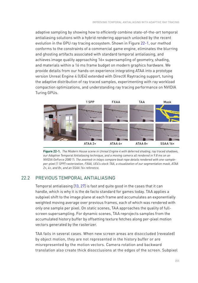
355
adaptive sampling by showing how to efficiently combine state-of-the- art temporal antialiasing solutions with a hybrid rendering approach unlocked by the recent evolution in the GPU ray tracing ecosystem. Shown in Figure 22-1, our method conforms to the constraints of a commercial game engine, eliminates the blurring and ghosting artifacts associated with standard temporal antialiasing, and achieves image quality approaching 16× supersampling of geometry, shading, and materials within a 16 ms frame budget on modern graphics hardware. We provide details from our hands-on experience integrating ATAA into a prototype version Unreal Engine 4 (UE4) extended with DirectX Raytracing support, tuning the adaptive distribution of ray traced samples, experimenting with ray workload compaction optimizations, and understanding ray tracing performance on NVIDIA Turing GPUs.
22.2 PREVIOUS TEMPORAL ANTIALIASING
Temporal antialiasing [13, 27] is fast and quite good in the cases that it can handle, which is why it is the de facto standard for games today. TAA applies a subpixel shift to the image plane at each frame and accumulates an exponentially weighted moving average over previous frames, each of which was rendered with only one sample per pixel. On static scenes, TAA approaches the quality of full-screen supersampling. For dynamic scenes, TAA reprojects samples from the accumulated history buffer by offsetting texture fetches along per-pixel motion vectors generated by the rasterizer.
TAA fails in several cases. When new screen areas are disoccluded (revealed) by object motion, they are not represented in the history buffer or are misrepresented by the motion vectors. Camera rotation and backward translation also create thick disocclusions at the edges of the screen. Subpixel
Figure 22-1. The Modern House scene in Unreal Engine 4 with deferred shading, ray traced shadows, our Adaptive Temporal Antialiasing technique, and a moving camera all rendered in 9.8 ms on an NVIDIA GeForce 2080 Ti. The zoomed-in inlays compare boat rope details rendered with one-sample-per-pixel (1 SPP) rasterization, FXAA, UE4’s stock TAA, a visualization of our segmentation mask, ATAA 2×, 4×, and 8×, and an SSAA 16× reference.
IMPROVING TEMPORAL ANTIALIASING WITH ADAPTIVE RAy TRACING
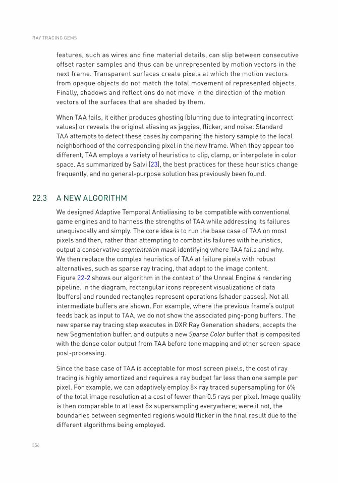
356
features, such as wires and fine material details, can slip between consecutive offset raster samples and thus can be unrepresented by motion vectors in the next frame. Transparent surfaces create pixels at which the motion vectors from opaque objects do not match the total movement of represented objects. Finally, shadows and reflections do not move in the direction of the motion vectors of the surfaces that are shaded by them.
When TAA fails, it either produces ghosting (blurring due to integrating incorrect values) or reveals the original aliasing as jaggies, flicker, and noise. Standard TAA attempts to detect these cases by comparing the history sample to the local neighborhood of the corresponding pixel in the new frame. When they appear too different, TAA employs a variety of heuristics to clip, clamp, or interpolate in color space. As summarized by Salvi [23], the best practices for these heuristics change frequently, and no general-purpose solution has previously been found.
22.3 A NEW ALGORITHM
We designed Adaptive Temporal Antialiasing to be compatible with conventional game engines and to harness the strengths of TAA while addressing its failures unequivocally and simply. The core idea is to run the base case of TAA on most pixels and then, rather than attempting to combat its failures with heuristics, output a conservative segmentation mask identifying where TAA fails and why. We then replace the complex heuristics of TAA at failure pixels with robust alternatives, such as sparse ray tracing, that adapt to the image content. Figure 22-2 shows our algorithm in the context of the Unreal Engine 4 rendering pipeline. In the diagram, rectangular icons represent visualizations of data (buffers) and rounded rectangles represent operations (shader passes). Not all intermediate buffers are shown. For example, where the previous frame’s output feeds back as input to TAA, we do not show the associated ping-pong buffers. The new sparse ray tracing step executes in DXR Ray Generation shaders, accepts the new Segmentation buffer, and outputs a new Sparse Color buffer that is composited with the dense color output from TAA before tone mapping and other screen-space post-processing.
Since the base case of TAA is acceptable for most screen pixels, the cost of ray tracing is highly amortized and requires a ray budget far less than one sample per pixel. For example, we can adaptively employ 8× ray traced supersampling for 6% of the total image resolution at a cost of fewer than 0.5 rays per pixel. Image quality is then comparable to at least 8× supersampling everywhere; were it not, the boundaries between segmented regions would flicker in the final result due to the different algorithms being employed.
RAY TRACING GEMS
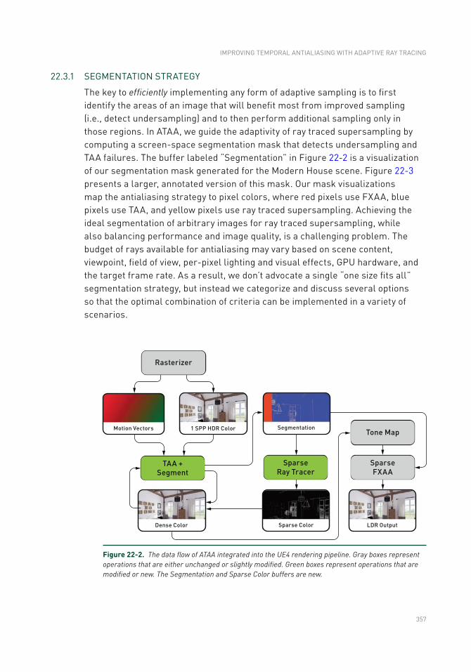
357
22.3.1 SEGMENTATION STRATEGy
The key to efficiently implementing any form of adaptive sampling is to first identify the areas of an image that will benefit most from improved sampling (i.e., detect undersampling) and to then perform additional sampling only in those regions. In ATAA, we guide the adaptivity of ray traced supersampling by computing a screen-space segmentation mask that detects undersampling and TAA failures. The buffer labeled “Segmentation” in Figure 22-2 is a visualization of our segmentation mask generated for the Modern House scene. Figure 22-3 presents a larger, annotated version of this mask. Our mask visualizations map the antialiasing strategy to pixel colors, where red pixels use FXAA, blue pixels use TAA, and yellow pixels use ray traced supersampling. Achieving the ideal segmentation of arbitrary images for ray traced supersampling, while also balancing performance and image quality, is a challenging problem. The budget of rays available for antialiasing may vary based on scene content, viewpoint, field of view, per-pixel lighting and visual effects, GPU hardware, and the target frame rate. As a result, we don’t advocate a single “one size fits all” segmentation strategy, but instead we categorize and discuss several options so that the optimal combination of criteria can be implemented in a variety of scenarios.
Figure 22-2. The data flow of ATAA integrated into the UE4 rendering pipeline. Gray boxes represent operations that are either unchanged or slightly modified. Green boxes represent operations that are modified or new. The Segmentation and Sparse Color buffers are new.
IMPROVING TEMPORAL ANTIALIASING WITH ADAPTIVE RAy TRACING
358
22.3.1.1 AUTOMATIC SEGMENTATION
Images can be effectively and efficiently segmented by inspecting the scene data available in screen space after rasterization. Since segmentation is generated algorithmically, without manual intervention from artists or developers, we refer to this process as automatic segmentation.
Modern rendering engines maintain per-pixel motion vectors, which we use during segmentation to determine if the current pixel was previously outside of the view (i.e., offscreen) or occluded by another surface. In the case of offscreen disocclusion, temporal raster data does not exist for use in antialiasing. Shown in Figure 22-3, we process these areas with FXAA (red), since it has a low cost, requires no historical data, and runs on the low dynamic range output, i.e., after tone mapping, to conserve memory bandwidth. By running FXAA only at offscreen disocclusion pixels, we further reduce its cost compared to full-screen applications, typically to less than 15% even for rapid camera movement. In the case of disocclusions from animated objects and skinned characters, temporal raster data exists but the shaded color is not representative of the currently visible surface. We eliminate common TAA ghosting artifacts and avoid aliasing caused by TAA clamping, as shown in Figure 22-4, by ignoring the temporal raster data and marking these pixels for ray traced supersampling (yellow). The result of inspecting motion vectors overrides all other criteria and may trigger an early exit in the segmentation process if either type of disocclusion is present. Now that TAA failures from disocclusions are handled, the segmentation process can turn to identifying areas of undersampling.
Figure 22-3. An annotated visualization of an ATAA segmentation mask. Blue pixels use standard TAA, red pixels use FXAA, and yellow pixels use ray traced supersampling.
RAY TRACING GEMS
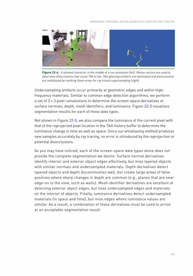
359
Undersampling artifacts occur primarily at geometric edges and within high- frequency materials. Similar to common edge detection algorithms, we perform a set of 3 × 3 pixel convolutions to determine the screen-space derivatives of surface normals, depth, mesh identifiers, and luminance. Figure 22-5 visualizes segmentation results for each of these data types.
Not shown in Figure 22-5, we also compare the luminance of the current pixel with that of the reprojected pixel location in the TAA history buffer to determine the luminance change in time as well as space. Since our antialiasing method produces new samples accurately by ray tracing, no error is introduced by the reprojection or potential disocclusions.
As you may have noticed, each of the screen-space data types alone does not provide the complete segmentation we desire. Surface normal derivatives identify interior and exterior object edges effectively, but miss layered objects with similar normals and undersampled materials. Depth derivatives detect layered objects and depth discontinuities well, but create large areas of false positives where sharp changes in depth are common (e.g., planes that are near edge-on to the view, such as walls). Mesh identifier derivatives are excellent at detecting exterior object edges, but miss undersampled edges and materials on the interior of objects. Finally, luminance derivatives detect undersampled materials (in space and time), but miss edges where luminance values are similar. As a result, a combination of these derivatives must be used to arrive at an acceptable segmentation result.
Figure 22-4. A skinned character in the middle of a run animation (left). Motion vectors are used to determine disocclusions that cause TAA to fail. TAA ghosting artifacts are eliminated and disocclusions are antialiased by marking these areas for ray traced supersampling (right).
IMPROVING TEMPORAL ANTIALIASING WITH ADAPTIVE RAy TRACING
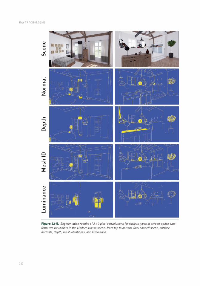
360
Figure 22-5. Segmentation results of 3 × 3 pixel convolutions for various types of screen-space data from two viewpoints in the Modern House scene: from top to bottom, final shaded scene, surface normals, depth, mesh identifiers, and luminance.
RAY TRACING GEMS
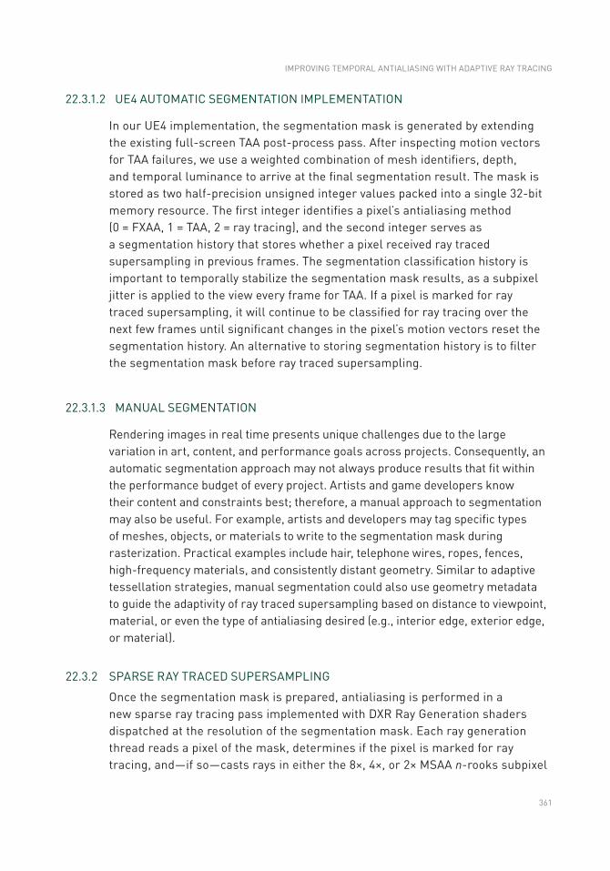
361
22.3.1.2 UE4 AUTOMATIC SEGMENTATION IMPLEMENTATION
In our UE4 implementation, the segmentation mask is generated by extending the existing full-screen TAA post-process pass. After inspecting motion vectors for TAA failures, we use a weighted combination of mesh identifiers, depth, and temporal luminance to arrive at the final segmentation result. The mask is stored as two half- precision unsigned integer values packed into a single 32-bit memory resource. The first integer identifies a pixel’s antialiasing method (0 = FXAA, 1 = TAA, 2 = ray tracing), and the second integer serves as a segmentation history that stores whether a pixel received ray traced supersampling in previous frames. The segmentation classification history is important to temporally stabilize the segmentation mask results, as a subpixel jitter is applied to the view every frame for TAA. If a pixel is marked for ray traced supersampling, it will continue to be classified for ray tracing over the next few frames until significant changes in the pixel’s motion vectors reset the segmentation history. An alternative to storing segmentation history is to filter the segmentation mask before ray traced supersampling.
22.3.1.3 MANUAL SEGMENTATION
Rendering images in real time presents unique challenges due to the large variation in art, content, and performance goals across projects. Consequently, an automatic segmentation approach may not always produce results that fit within the performance budget of every project. Artists and game developers know their content and constraints best; therefore, a manual approach to segmentation may also be useful. For example, artists and developers may tag specific types of meshes, objects, or materials to write to the segmentation mask during rasterization. Practical examples include hair, telephone wires, ropes, fences, high-frequency materials, and consistently distant geometry. Similar to adaptive tessellation strategies, manual segmentation could also use geometry metadata to guide the adaptivity of ray traced supersampling based on distance to viewpoint, material, or even the type of antialiasing desired (e.g., interior edge, exterior edge, or material).
22.3.2 SPARSE RAy TRACED SUPERSAMPLING
Once the segmentation mask is prepared, antialiasing is performed in a new sparse ray tracing pass implemented with DXR Ray Generation shaders dispatched at the resolution of the segmentation mask. Each ray generation thread reads a pixel of the mask, determines if the pixel is marked for ray tracing, and—if so—casts rays in either the 8×, 4×, or 2× MSAA n-rooks subpixel
IMPROVING TEMPORAL ANTIALIASING WITH ADAPTIVE RAy TRACING
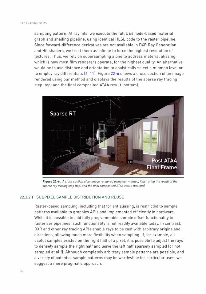
362
sampling pattern. At ray hits, we execute the full UE4 node-based material graph and shading pipeline, using identical HLSL code to the raster pipeline. Since forward-difference derivatives are not available in DXR Ray Generation and Hit shaders, we treat them as infinite to force the highest resolution of textures. Thus, we rely on supersampling alone to address material aliasing, which is how most film renderers operate, for the highest quality. An alternative would be to use distance and orientation to analytically select a mipmap level or to employ ray differentials [6, 11]. Figure 22-6 shows a cross section of an image rendered using our method and displays the results of the sparse ray tracing step (top) and the final composited ATAA result (bottom).
Figure 22-6. A cross section of an image rendered using our method, illustrating the result of the sparse ray tracing step (top) and the final composited ATAA result (bottom).
22.3.2.1 SUBPIXEL SAMPLE DISTRIBUTION AND REUSE
Raster-based sampling, including that for antialiasing, is restricted to sample patterns available to graphics APIs and implemented efficiently in hardware. While it is possible to add fully programmable sample offset functionality to rasterizer pipelines, such functionality is not readily available today. In contrast, DXR and other ray tracing APIs enable rays to be cast with arbitrary origins and directions, allowing much more flexibility when sampling. If, for example, all useful samples existed on the right half of a pixel, it is possible to adjust the rays to densely sample the right half and leave the left half sparsely sampled (or not sampled at all!). Although completely arbitrary sample patterns are possible, and a variety of potential sample patterns may be worthwhile for particular uses, we suggest a more pragmatic approach.
RAY TRACING GEMS
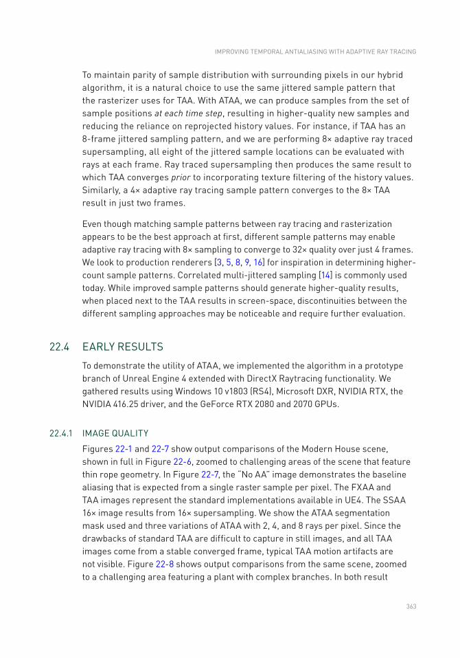
363
To maintain parity of sample distribution with surrounding pixels in our hybrid algorithm, it is a natural choice to use the same jittered sample pattern that the rasterizer uses for TAA. With ATAA, we can produce samples from the set of sample positions at each time step, resulting in higher-quality new samples and reducing the reliance on reprojected history values. For instance, if TAA has an 8-frame jittered sampling pattern, and we are performing 8× adaptive ray traced supersampling, all eight of the jittered sample locations can be evaluated with rays at each frame. Ray traced supersampling then produces the same result to which TAA converges prior to incorporating texture filtering of the history values. Similarly, a 4× adaptive ray tracing sample pattern converges to the 8× TAA result in just two frames.
Even though matching sample patterns between ray tracing and rasterization appears to be the best approach at first, different sample patterns may enable adaptive ray tracing with 8× sampling to converge to 32× quality over just 4 frames. We look to production renderers [3, 5, 8, 9, 16] for inspiration in determining higher-count sample patterns. Correlated multi-jittered sampling [14] is commonly used today. While improved sample patterns should generate higher-quality results, when placed next to the TAA results in screen-space, discontinuities between the different sampling approaches may be noticeable and require further evaluation.
22.4 EARLy RESULTS
To demonstrate the utility of ATAA, we implemented the algorithm in a prototype branch of Unreal Engine 4 extended with DirectX Raytracing functionality. We gathered results using Windows 10 v1803 (RS4), Microsoft DXR, NVIDIA RTX, the NVIDIA 416.25 driver, and the GeForce RTX 2080 and 2070 GPUs.
22.4.1 IMAGE QUALITy
Figures 22-1 and 22-7 show output comparisons of the Modern House scene, shown in full in Figure 22-6, zoomed to challenging areas of the scene that feature thin rope geometry. In Figure 22-7, the “No AA” image demonstrates the baseline aliasing that is expected from a single raster sample per pixel. The FXAA and TAA images represent the standard implementations available in UE4. The SSAA 16× image results from 16× supersampling. We show the ATAA segmentation mask used and three variations of ATAA with 2, 4, and 8 rays per pixel. Since the drawbacks of standard TAA are difficult to capture in still images, and all TAA images come from a stable converged frame, typical TAA motion artifacts are not visible. Figure 22-8 shows output comparisons from the same scene, zoomed to a challenging area featuring a plant with complex branches. In both result
IMPROVING TEMPORAL ANTIALIASING WITH ADAPTIVE RAy TRACING
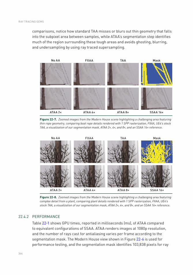
364
Figure 22-8. Zoomed images from the Modern House scene highlighting a challenging area featuring complex detail from a plant, comparing plant details rendered with 1 SPP rasterization, FXAA, UE4’s stock TAA, a visualization of our segmentation mask, ATAA 2×, 4×, and 8×, and an SSAA 16× reference.
comparisons, notice how standard TAA misses or blurs out thin geometry that falls into the subpixel area between samples, while ATAA’s segmentation step identifies much of the region surrounding these tough areas and avoids ghosting, blurring, and undersampling by using ray traced supersampling.
Figure 22-7. Zoomed images from the Modern House scene highlighting a challenging area featuring thin rope geometry, comparing boat rope details rendered with 1 SPP rasterization, FXAA, UE4’s stock TAA, a visualization of our segmentation mask, ATAA 2×, 4×, and 8×, and an SSAA 16× reference.
22.4.2 PERFORMANCE
Table 22-1 shows GPU times, reported in milliseconds (ms), of ATAA compared to equivalent configurations of SSAA. ATAA renders images at 1080p resolution, and the number of rays cast for antialiasing varies per frame according to the segmentation mask. The Modern House view shown in Figure 22-6 is used for performance testing, and the segmentation mask identifies 103,838 pixels for ray
RAY TRACING GEMS
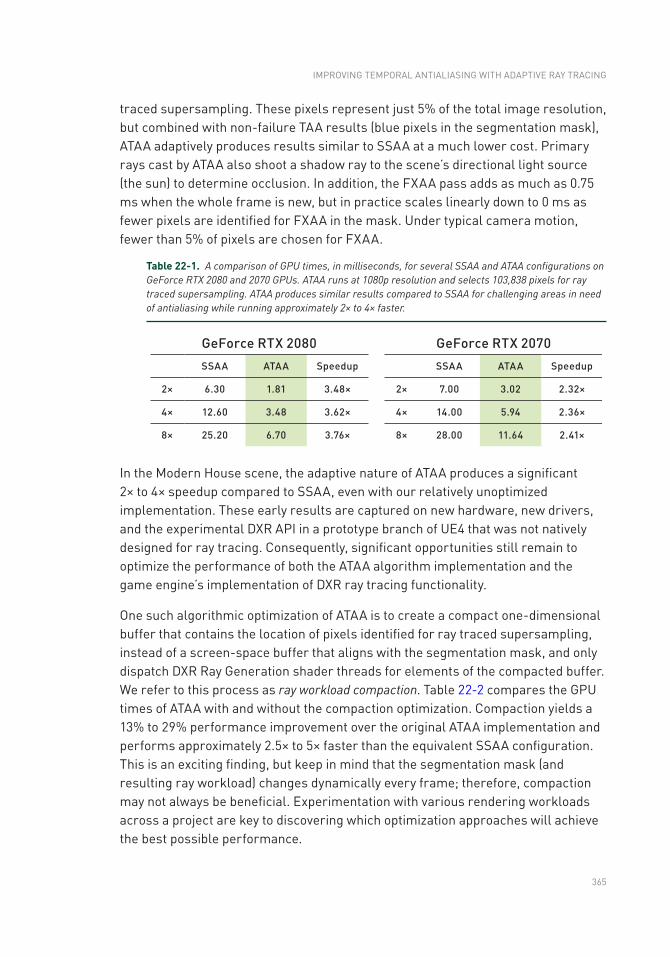
365
traced supersampling. These pixels represent just 5% of the total image resolution, but combined with non-failure TAA results (blue pixels in the segmentation mask), ATAA adaptively produces results similar to SSAA at a much lower cost. Primary rays cast by ATAA also shoot a shadow ray to the scene’s directional light source (the sun) to determine occlusion. In addition, the FXAA pass adds as much as 0.75 ms when the whole frame is new, but in practice scales linearly down to 0 ms as fewer pixels are identified for FXAA in the mask. Under typical camera motion, fewer than 5% of pixels are chosen for FXAA.
Table 22-1. A comparison of GPU times, in milliseconds, for several SSAA and ATAA configurations on GeForce RTX 2080 and 2070 GPUs. ATAA runs at 1080p resolution and selects 103,838 pixels for ray traced supersampling. ATAA produces similar results compared to SSAA for challenging areas in need of antialiasing while running approximately 2× to 4× faster.
In the Modern House scene, the adaptive nature of ATAA produces a significant 2× to 4× speedup compared to SSAA, even with our relatively unoptimized implementation. These early results are captured on new hardware, new drivers, and the experimental DXR API in a prototype branch of UE4 that was not natively designed for ray tracing. Consequently, significant opportunities still remain to optimize the performance of both the ATAA algorithm implementation and the game engine’s implementation of DXR ray tracing functionality.
One such algorithmic optimization of ATAA is to create a compact one-dimensional buffer that contains the location of pixels identified for ray traced supersampling, instead of a screen-space buffer that aligns with the segmentation mask, and only dispatch DXR Ray Generation shader threads for elements of the compacted buffer. We refer to this process as ray workload compaction. Table 22-2 compares the GPU times of ATAA with and without the compaction optimization. Compaction yields a 13% to 29% performance improvement over the original ATAA implementation and performs approximately 2.5× to 5× faster than the equivalent SSAA configuration. This is an exciting finding, but keep in mind that the segmentation mask (and resulting ray workload) changes dynamically every frame; therefore, compaction may not always be beneficial. Experimentation with various rendering workloads across a project are key to discovering which optimization approaches will achieve the best possible performance.
IMPROVING TEMPORAL ANTIALIASING WITH ADAPTIVE RAy TRACING
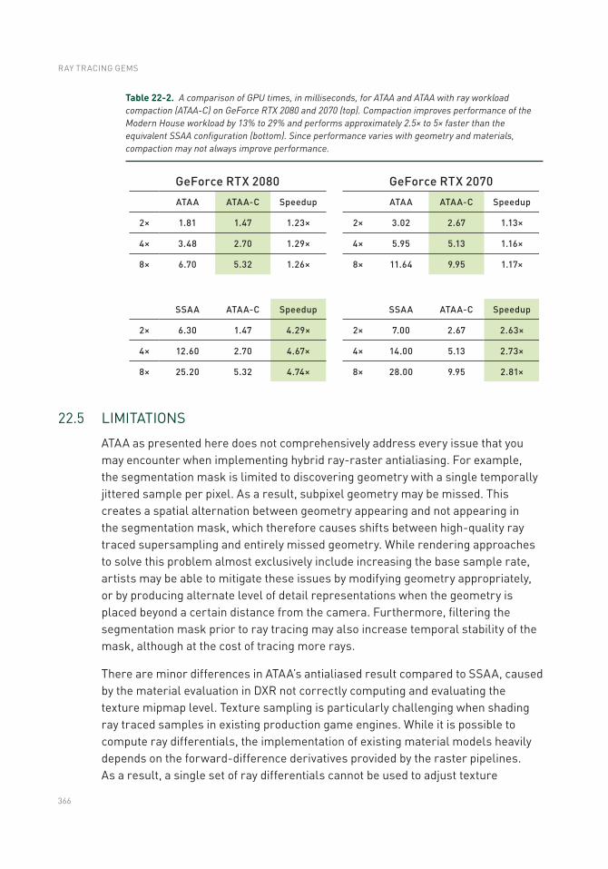
366
Table 22-2. A comparison of GPU times, in milliseconds, for ATAA and ATAA with ray workload compaction (ATAA-C) on GeForce RTX 2080 and 2070 (top). Compaction improves performance of the Modern House workload by 13% to 29% and performs approximately 2.5× to 5× faster than the equivalent SSAA configuration (bottom). Since performance varies with geometry and materials, compaction may not always improve performance.
22.5 LIMITATIONS
ATAA as presented here does not comprehensively address every issue that you may encounter when implementing hybrid ray-raster antialiasing. For example, the segmentation mask is limited to discovering geometry with a single temporally jittered sample per pixel. As a result, subpixel geometry may be missed. This creates a spatial alternation between geometry appearing and not appearing in the segmentation mask, which therefore causes shifts between high-quality ray traced supersampling and entirely missed geometry. While rendering approaches to solve this problem almost exclusively include increasing the base sample rate, artists may be able to mitigate these issues by modifying geometry appropriately, or by producing alternate level of detail representations when the geometry is placed beyond a certain distance from the camera. Furthermore, filtering the segmentation mask prior to ray tracing may also increase temporal stability of the mask, although at the cost of tracing more rays.
There are minor differences in ATAA’s antialiased result compared to SSAA, caused by the material evaluation in DXR not correctly computing and evaluating the texture mipmap level. Texture sampling is particularly challenging when shading ray traced samples in existing production game engines. While it is possible to compute ray differentials, the implementation of existing material models heavily depends on the forward-difference derivatives provided by the raster pipelines. As a result, a single set of ray differentials cannot be used to adjust texture
RAY TRACING GEMS
367
mipmap level when sampling, making the ray differential computation especially costly. In our implementation, all ray samples select the highest-frequency texture. This limitation results in texture aliasing in many cases, but at higher sample counts we are able to reconstruct the appropriate filtered result. Additionally, TAA history and new raster samples have filtered texture sampling, which can be blended with our ray traced samples to mitigate texture aliasing.
Another practical difficulty for ray traced antialiasing of primary visibility is supporting screen-space effects. Since rays are distributed sparsely across screen space, there is no guarantee the necessary data that post-process effects such as depth of field, motion blur, and lens flare use will exist in nearby pixels. A simple solution is to move the antialiasing step before these passes, at the cost of these effects not benefiting from additional antialiasing. In the long term, as the budget of ray samples increases, it may be sensible to move the raster-based screen-space effects to ray traced equivalents.
22.6 THE FUTURE OF REAL-TIME RAy TRACED ANTIALIASING
The recent arrival of graphics processors with dedicated acceleration for ray tracing creates an opportunity to reassess the state of the art, and in turn reinvent real-time antialiasing. This chapter presents implementation details beyond the initial publication of ATAA [18] and may serve as a foundation upon which production renderers of the future build. A primary remaining concern for production deployment is ensuring that the runtime of the sparse ray tracing pass fits within the available frame time budget. Once the pixels for ray traced supersampling are selected, we suggest pursuing additional heuristics to adjust performance, including naively dropping rays after the target number is hit, deprioritizing rays in screen-space regions where aliasing is less common or perceptually less important, and selecting ray counts based on a priority metric embedded in the segmentation mask. We expect adjusting ray counts per pixel will improve ray tracing performance in a given region of interest. Due to the SIMD architecture of current GPUs, these adjustments are optimally made on warp boundaries, thus pixels requiring similar sample counts may benefit from being placed together when spawning work, a task that can also be completed during a workload compaction pass.
IMPROVING TEMPORAL ANTIALIASING WITH ADAPTIVE RAy TRACING
368
22.7 CONCLUSION
Primary surface aliasing is a cornerstone problem in computer graphics. The best- known solution for offline rendering is adaptive supersampling. This was previously impractical for rasterization renderers in the context of complex materials and scenes because there was no way to efficiently rasterize sparse pixels. Even the most efficient GPU ray tracers required duplicated shaders and scene data. While DXR solves the technical challenge of combining rasterization and ray tracing, applying ray tracing to solve aliasing by supersampling is nontrivial: knowing which pixels to supersample when given only 1 SPP input and reducing the cost to something that scales are not solved by naively ray tracing.
We have demonstrated a practical solution to this problem—so practical that it runs within a commercial game engine, operates in real time even on first-generation real-time ray tracing commodity hardware and software, and connects to the full shader pipeline. Where film renderers choose pixels to adaptively supersample by first casting many rays per pixel, we instead amortize that cost over many frames by leveraging TAA’s history buffer to detect aliasing. We further identify large, transient regions of aliasing due to disocclusions and employ post-process FXAA there rather than expending rays. This hybrid strategy leverages advantages of the most sophisticated real-time antialiasing strategies while eliminating many of their limitations. By feeding our supersampled results back into the TAA buffer, we also increase the probability that those pixels will not trigger supersampling on subsequent frames, further reducing cost.
REFERENCES
[1] Auzinger, T., Musialski, P., Preiner, R., and Wimmer, M. Non-Sampled Anti-Aliasing. In Vision, Modeling and Visualization (2013), pp. 169–176.
[2] Barringer, R., and Akenine-Möller, T. A4: Asynchronous Adaptive Anti-Aliasing Using Shared Memory. ACM Transactions on Graphics 32, 4 (July 2013), 100:1–100:10.
[3] Burley, B., Adler, D., Chiang, M. J.-y., Driskill, H., Habel, R., Kelly, P., Kutz, P., Li, y. K., and Teece, D. The Design and Evolution of Disneys Hyperion Renderer. ACM Transactions on Graphics 37, 3 (2018), 33:1–33:22.
[4] Chajdas, M. G., McGuire, M., and Luebke, D. Subpixel Reconstruction Antialiasing for Deferred Shading. In Symposium on Interactive 3D Graphics and Games (2011), pp. 15–22.
[5] Christensen, P., Fong, J., Shade, J., Wooten, W., Schubert, B., Kensler, A., Friedman, S., Kilpatrick, C., Ramshaw, C., Bannister, M., Rayner, B., Brouillat, J., and Liani, M. RenderMan: An Advanced Path-Tracing Architecture for Movie Rendering. ACM Transactions on Graphics 37, 3 (2018), 30:1–30:21.
RAY TRACING GEMS
369
[6] Christensen, P. H., Laur, D. M., Fong, J., Wooten, W. L., and Batali, D. Ray Differentials and Multiresolution Geometry Caching for Distribution Ray Tracing in Complex Scenes. Computer Graphics Forum 22, 3 (2003), 543–552.
[7] Crassin, C., McGuire, M., Fatahalian, K., and Lefohn, A. Aggregate G-Buffer Anti- Aliasing. IEEE Transactions on Visualization and Computer Graphics 22, 10 (2016), 2215–2228.
[8] Fascione, L., Hanika, J., Leone, M., Droske, M., Schwarzhaupt, J., Davidovic , T., Weidlich, A., and Meng, J. Manuka: A Batch-Shading Architecture for Spectral Path Tracing in Movie Production. ACM Transactions on Graphics 37, 3 (2018), 31:1–31:18.
[9] Georgiev, I., Ize, T., Farnsworth, M., Montoya-Vozmediano, R., King, A., Lommel, B. V., Jimenez, A., Anson, O., Ogaki, S., Johnston, E., Herubel, A., Russell, D., Servant, F., and Fajardo, M. Arnold: A Brute-Force Production Path Tracer. ACM Transactions on Graphics 37, 3 (2018), 32:1–32:12.
[10] Holländer, M., Boubekeur, T., and Eisemann, E. Adaptive Supersampling for Deferred Anti-Aliasing. Journal of Computer Graphics Techniques 2, 1 (March 2013), 1–14.
[11] Igehy, H. Tracing Ray Differentials. In Proceedings of SIGGRAPH (1999), pp. 179–186.
[12] Jimenez, J., Echevarria, J. I., Sousa, T., and Gutierrez, D. SMAA: Enhanced Morphological Antialiasing. Computer Graphics Forum 31, 2 (2012), 355–364.
[13] Karis, B. High Quality Temporal Anti-Aliasing. Advances in Real-Time Rendering for Games, SIGGRAPH Courses, 2014.
[14] Kensler, A. Correlated Multi-Jittered Sampling. Pixar Technical Memo 13-01, 2013.
[15] Kobbelt, L., and Botsch, M. A Survey of Point-Based Techniques in Computer Graphics. Computers and Graphics 28, 6 (Dec. 2004), 801–814.
[16] Kulla, C., Conty, A., Stein, C., and Gritz, L. Sony Pictures Imageworks Arnold. ACM Transactions on Graphics 37, 3 (2018), 29:1–29:18.
[17] Lottes, T. FXAA. NVIDIA White Paper, 2009.
[18] Marrs, A., Spjut, J., Gruen, H., Sathe, R., and McGuire, M. Adaptive Temporal Antialiasing. In Proceedings of High-Performance Graphics (2018), pp. 1:1–1:4.
[19] Olano, M., and Baker, D. LEAN Mapping. In Symposium on Interactive 3D Graphics and Games (2010), pp. 181–188.
[20] Pedersen, L. J. F. Temporal Reprojection Anti-Aliasing in INSIDE. Game Developers Conference, 2016.
[21] Pettineo, M. Rendering the Alternate History of The Order: 1886. Advances in Real- Time Rendering in Games, SIGGRAPH Courses, 2015.
[22] Reshetov, A. Morphological Antialiasing. In Proceedings of High-Performance Graphics (2009), pp. 109–116.
[23] Salvi, M. Anti-Aliasing: Are We There yet? Open Problems in Real-Time Rendering, SIGGRAPH Courses, 2015.
[24] Salvi, M., and Vidimce, K. Surface Based Anti-Aliasing. In Symposium on Interactive 3D Graphics and Games (2012), pp. 159–164.
IMPROVING TEMPORAL ANTIALIASING WITH ADAPTIVE RAy TRACING

370
[25] Wang, y., Wyman, C., He, y., and Sen, P. Decoupled Coverage Anti-Aliasing. In Proceedings of High-Performance Graphics (2015), pp. 33–42.
[26] Whitted, T. An Improved Illumination Model for Shaded Display. Communications of the ACM 23, 6 (June 1980), 343–349.
[27] yang, L., Nehab, D., Sander, P. V., Sitthi-amorn, P., Lawrence, J., and Hoppe, H. Amortized Supersampling. ACM Transactions on Graphics 28, 5 (Dec. 2009), 135:1–135:12.
Open Access This chapter is licensed under the terms of the Creative Commons Attribution-NonCommercial-NoDerivatives 4.0 International License (http://creativecommons.org/licenses/by-nc-nd/4.0/), which permits any noncommercial use, sharing, distribution and
reproduction in any medium or format, as long as you give appropriate credit to the original author(s) and the source, provide a link to the Creative Commons license and indicate if you modified the licensed material. you do not have permission under this license to share adapted material derived from this chapter or parts of it.
The images or other third party material in this chapter are included in the chapter's Creative Commons license, unless indicated otherwise in a credit line to the material. If material is not included in the chapter's Creative Commons license and your intended use is not permitted by statutory regulation or exceeds the permitted use, you will need to obtain permission directly from the copyright holder.
RAY TRACING GEMS
PART VI
HYBRID APPROACHES AND SYSTEMS
375
PART VI
Hybrid Approaches and Systems
Sometimes a “gem” is more than just a good algorithm or implementation—it is a design for a system. The chapters in this part of the book present five systems for hybrid rendering using GPU ray tracing and rasterization together. They cover a range of application targets and scales to provide good ideas for every real-time rendering program.
Chapter 23, “Interactive Light Map and Irradiance Volume Preview in Frostbite,” presents a comprehensive tool for using ray tracing to speed entertainment production. For two decades, film and game artists’ lighting workflow frequently has been limited by the long process of “baking” global illumination. In this chapter the Frostbite game engine team describes in detail their hybrid rendering system for rapid previewing of full global illumination.
Chapter 24, “Real-Time Global Illumination with Photon Mapping,” describes a method for simulating global illumination by tracing light forward from the emitters and then applying it to surfaces rasterized or ray traced backward from the camera. This system can handle cases such as bright caustics caused by specular reflection and refraction for which path tracing is slow to converge. More importantly, it provides a stable way of caching and amortizing light paths across many pixels.
Chapter 25, “Hybrid Rendering for Real-Time Ray Tracing,” gives the implementation details and lessons learned from the PICA PICA demo produced by the SEED game developer research group at Electronic Arts. It is a comprehensive system for global illumination within game-like resource constraints. The chapter presents targeted methods for ray tracing transparency, ambient occlusion, primary shadows, glossy reflection, and diffuse interreflection, and then describes how to combine them with rasterization into a complete hybrid rendering system.
Chapter 26, “Deferred Hybrid Path Tracing,” presents a path tracer using aggressive new spatial data structure radiance caching techniques. It produces high-quality interactive flythrough renderings of static scenes using only seconds of precomputation suitable for the authors’ architectural visualization application.

376
Chapter 27, “Interactive Ray Tracing Techniques for High-Fidelity Scientific Visualization,” describes multiple ray tracing techniques appropriate for scientific visualization, where the combination of high quality and interactivity can enable new insights for domain experts without computer graphics expertise.
These chapters show how ray tracing has become a powerful tool in the toolchest, both for interactive rendering and fast previewing of baked effects. Improving the speed and ease of use of operations such as BVH traversal and ray/triangle intersection opens up new opportunities. Expect to see much more research and development of hybrid approaches in the years ahead.
Morgan McGuire
377© NVIDIA 2019 E. Haines, T. Akenine-Möller (eds.), Ray Tracing Gems, https://doi.org/10.1007/978-1-4842-4427-2_23
CHAPTER 23
Interactive Light Map and Irradiance Volume Preview in FrostbiteDiede Apers, Petter Edblom, Charles de Rousiers, and Sébastien HillaireElectronic Arts
ABSTRACT
This chapter presents the real-time global illumination (GI) preview system available in the Frostbite engine. Our approach is based on Monte Carlo path tracing running on the GPU, built using the DirectX Raytracing (DXR) API. We present an approach to updating light maps and irradiance volumes in real time according to elements constituting a scene. Methods to accelerate these updates, such as view prioritization and irradiance caching, are also described. A light map denoiser is used to always present a pleasing image on screen. This solution allows artists to visualize the result of their edits, progressively refined on screen, rather than waiting minutes to hours for the final result using the previous CPU-based GI solver. Even if the GI solution being refined in real time on screen has not converged after a few seconds, it is enough for artists to get an idea of the final look and assess the scene quality. It enables them to iterate faster and so achieve a higher-quality scene lighting setup.
23.1 INTRODUCTION
Precomputed lighting using light maps has been used in games since Quake in 1996. From there, light map representations have evolved to reach higher visual fidelity [1, 8]. However, their use in production is still constrained by long baking times, making the lighting workflow inefficient for artists and difficult for engineers to debug. Our goal is to provide a real-time preview of diffuse GI within the Frostbite editor.
Electronic Arts produces various types of games relying on a wide range of lighting complexities: static lighting such as in Star Wars Battlefront 2, dynamic sunlight for time of day simulation such as in Need for Speed, and even destruction requiring dynamic updates of the GI solution from dynamic lights such as in the Battlefield series. This chapter focuses on the static GI case, i.e., unchanging GI during gameplay, for which Frostbite’s own GI solver can be used [9]. See Figure 23-1. Static GI relying on baked light maps and probes will always be a good value: it
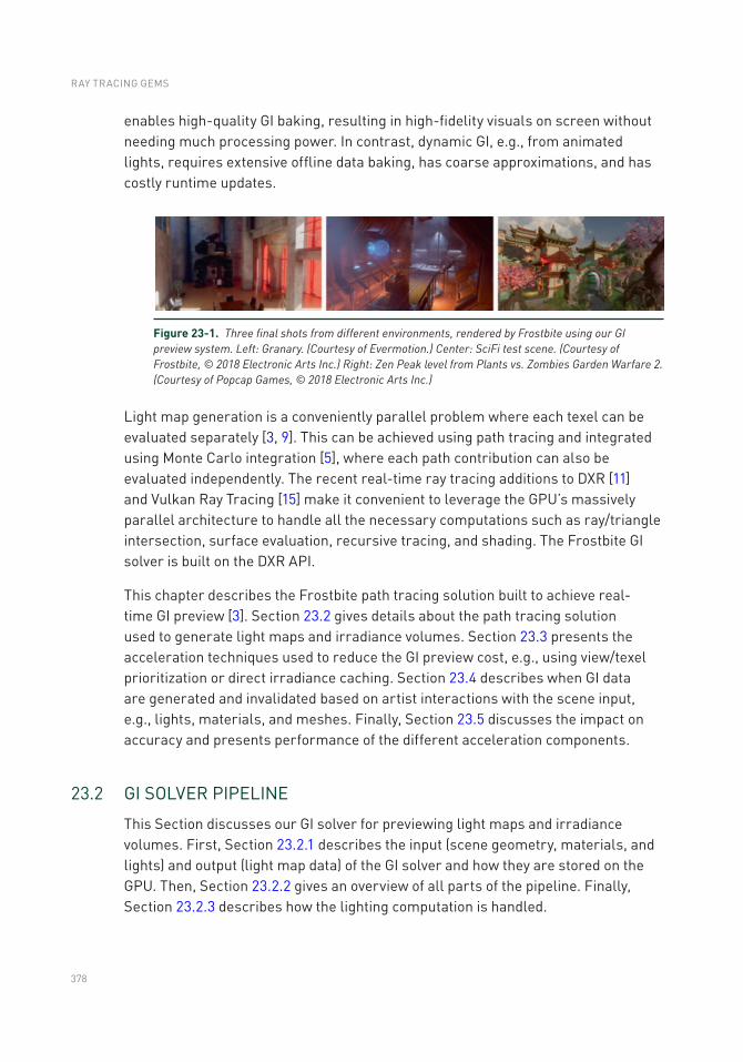
378
enables high-quality GI baking, resulting in high-fidelity visuals on screen without needing much processing power. In contrast, dynamic GI, e.g., from animated lights, requires extensive offline data baking, has coarse approximations, and has costly runtime updates.
Figure 23-1. Three final shots from different environments, rendered by Frostbite using our GI preview system. Left: Granary. (Courtesy of Evermotion.) Center: SciFi test scene. (Courtesy of Frostbite, © 2018 Electronic Arts Inc.) Right: Zen Peak level from Plants vs. Zombies Garden Warfare 2. (Courtesy of Popcap Games, © 2018 Electronic Arts Inc.)
Light map generation is a conveniently parallel problem where each texel can be evaluated separately [3, 9]. This can be achieved using path tracing and integrated using Monte Carlo integration [5], where each path contribution can also be evaluated independently. The recent real-time ray tracing additions to DXR [11] and Vulkan Ray Tracing [15] make it convenient to leverage the GPU’s massively parallel architecture to handle all the necessary computations such as ray/triangle intersection, surface evaluation, recursive tracing, and shading. The Frostbite GI solver is built on the DXR API.
This chapter describes the Frostbite path tracing solution built to achieve real-time GI preview [3]. Section 23.2 gives details about the path tracing solution used to generate light maps and irradiance volumes. Section 23.3 presents the acceleration techniques used to reduce the GI preview cost, e.g., using view/texel prioritization or direct irradiance caching. Section 23.4 describes when GI data are generated and invalidated based on artist interactions with the scene input, e.g., lights, materials, and meshes. Finally, Section 23.5 discusses the impact on accuracy and presents performance of the different acceleration components.
23.2 GI SOLVER PIPELINE
This Section discusses our GI solver for previewing light maps and irradiance volumes. First, Section 23.2.1 describes the input (scene geometry, materials, and lights) and output (light map data) of the GI solver and how they are stored on the GPU. Then, Section 23.2.2 gives an overview of all parts of the pipeline. Finally, Section 23.2.3 describes how the lighting computation is handled.
RAY TRACING GEMS
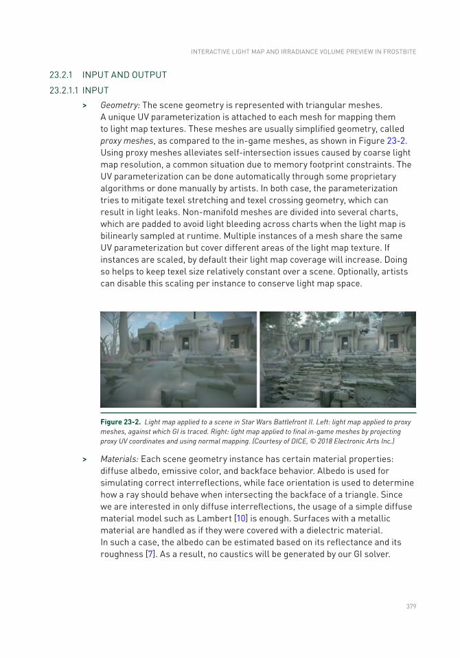
379
23.2.1 INPUT AND OUTPUT
23.2.1.1 INPUT
> Geometry: The scene geometry is represented with triangular meshes. A unique UV parameterization is attached to each mesh for mapping them to light map textures. These meshes are usually simplified geometry, called proxy meshes, as compared to the in- game meshes, as shown in Figure 23-2. Using proxy meshes alleviates self-intersection issues caused by coarse light map resolution, a common situation due to memory footprint constraints. The UV parameterization can be done automatically through some proprietary algorithms or done manually by artists. In both case, the parameterization tries to mitigate texel stretching and texel crossing geometry, which can result in light leaks. Non-manifold meshes are divided into several charts, which are padded to avoid light bleeding across charts when the light map is bilinearly sampled at runtime. Multiple instances of a mesh share the same UV parameterization but cover different areas of the light map texture. If instances are scaled, by default their light map coverage will increase. Doing so helps to keep texel size relatively constant over a scene. Optionally, artists can disable this scaling per instance to conserve light map space.
Figure 23-2. Light map applied to a scene in Star Wars Battlefront II. Left: light map applied to proxy meshes, against which GI is traced. Right: light map applied to final in-game meshes by projecting proxy UV coordinates and using normal mapping. (Courtesy of DICE, © 2018 Electronic Arts Inc.)
> Materials: Each scene geometry instance has certain material properties: diffuse albedo, emissive color, and backface behavior. Albedo is used for simulating correct interreflections, while face orientation is used to determine how a ray should behave when intersecting the backface of a triangle. Since we are interested in only diffuse interreflections, the usage of a simple diffuse material model such as Lambert [10] is enough. Surfaces with a metallic material are handled as if they were covered with a dielectric material. In such a case, the albedo can be estimated based on its reflectance and its roughness [7]. As a result, no caustics will be generated by our GI solver.
INTERACTIVE LIGHT MAP AND IRRADIANCE VOLUME PREVIEW IN FROSTBITE
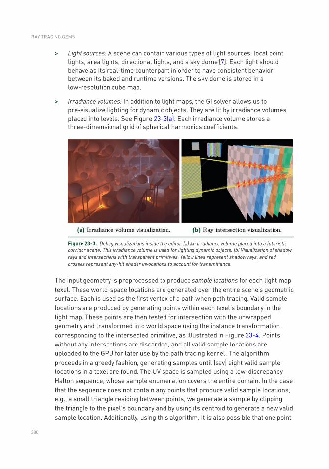
380
> Light sources: A scene can contain various types of light sources: local point lights, area lights, directional lights, and a sky dome [7]. Each light should behave as its real-time counterpart in order to have consistent behavior between its baked and runtime versions. The sky dome is stored in a low-resolution cube map.
> Irradiance volumes: In addition to light maps, the GI solver allows us to pre-visualize lighting for dynamic objects. They are lit by irradiance volumes placed into levels. See Figure 23-3(a). Each irradiance volume stores a three-dimensional grid of spherical harmonics coefficients.
The input geometry is preprocessed to produce sample locations for each light map texel. These world-space locations are generated over the entire scene’s geometric surface. Each is used as the first vertex of a path when path tracing. Valid sample locations are produced by generating points within each texel’s boundary in the light map. These points are then tested for intersection with the unwrapped geometry and transformed into world space using the instance transformation corresponding to the intersected primitive, as illustrated in Figure 23-4. Points without any intersections are discarded, and all valid sample locations are uploaded to the GPU for later use by the path tracing kernel. The algorithm proceeds in a greedy fashion, generating samples until (say) eight valid sample locations in a texel are found. The UV space is sampled using a low-discrepancy Halton sequence, whose sample enumeration covers the entire domain. In the case that the sequence does not contain any points that produce valid sample locations, e.g., a small triangle residing between points, we generate a sample by clipping the triangle to the pixel’s boundary and by using its centroid to generate a new valid sample location. Additionally, using this algorithm, it is also possible that one point
Figure 23-3. Debug visualizations inside the editor. (a) An irradiance volume placed into a futuristic corridor scene. This irradiance volume is used for lighting dynamic objects. (b) Visualization of shadow rays and intersections with transparent primitives. Yellow lines represent shadow rays, and red crosses represent any-hit shader invocations to account for transmittance.
RAY TRACING GEMS
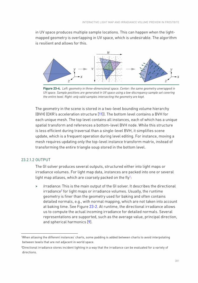
381
in UV space produces multiple sample locations. This can happen when the light- mapped geometry is overlapping in UV space, which is undesirable. The algorithm is resilient and allows for this.
The geometry in the scene is stored in a two-level bounding volume hierarchy (BVH) (DXR’s acceleration structure [11]). The bottom level contains a BVH for each unique mesh. The top level contains all instances, each of which has a unique spatial transform and references a bottom-level BVH node. While this structure is less efficient during traversal than a single-level BVH, it simplifies scene update, which is a frequent operation during level editing. For instance, moving a mesh requires updating only the top-level instance transform matrix, instead of transforming the entire triangle soup stored in the bottom level.
23.2.1.2 OUTPUT
The GI solver produces several outputs, structured either into light maps or irradiance volumes. For light map data, instances are packed into one or several light map atlases, which are coarsely packed on the fly1:
> Irradiance: This is the main output of the GI solver. It describes the directional irradiance2 for light maps or irradiance volumes. Usually, the runtime geometry is finer than the geometry used for baking and often contains detailed normals, e.g., with normal mapping, which are not taken into account at baking time. See Figure 23-2. At runtime, the directional irradiance allows us to compute the actual incoming irradiance for detailed normals. Several representations are supported, such as the average value, principal direction, and spherical harmonics [9].
1 When atlasing the different instances’ charts, some padding is added between charts to avoid interpolating between texels that are not adjacent in world space.
2 Directional irradiance stores incident lighting in a way that the irradiance can be evaluated for a variety of directions.
Figure 23-4. Left: geometry in three-dimensional space. Center: the same geometry unwrapped in UV space. Sample positions are generated in UV space using a low-discrepancy sample set covering the entire texel. Right: only valid samples intersecting the geometry are kept.
INTERACTIVE LIGHT MAP AND IRRADIANCE VOLUME PREVIEW IN FROSTBITE
382
> Sky visibility: This describes the portion of the sky visible from a given light map texel or irradiance volume point [7]. This value is used at runtime for various purposes, such as reflection blending or material effects.
> Ambient occlusion: This describes the surrounding occlusion for a given light map texel or irradiance volume point [7]. It is used at runtime for reflection occlusion.
23.2.2 GI SOLVER PIPELINE OVERVIEW
The proposed pipeline aims to preview the final outputs as quickly as possible. Since computing fully converged outputs would likely take several seconds or minutes for a production-size level, the proposed pipeline refines the outputs iteratively, as seen in Figure 23-5. At each solving iteration, the following operations are done:
> Update scene: All scene modifications since the last iteration are applied, e.g., moving a mesh or changing a light’s color. These inputs are translated and uploaded to the GPU. See Section 23.4.
> Update caches: If invalidated or incomplete, the irradiance caches are refined by tracing additional rays for estimating the incident direct irradiance. These caches are used for accelerating the tracing step. See Section 23.3.3.
> Schedule texels: Based on the camera’s view frustum, the most relevant visible light map texels and visible irradiance volumes are identified and scheduled for the tracing step. See Section 23.3.1.
> Trace texels: Each scheduled texel and irradiance point is refined by tracing a set of paths. These paths allow one to compute the incoming irradiance, as well as sky visibility and ambient occlusion. See Section 23.2.3.
> Merge texels: The newly computed irradiance samples are accumulated into persistent output resources. See Section 23.2.6.
> Post-process outputs: Dilation and denoising post-process passes are applied to the outputs, giving users a noise-free estimate of the converged output. See Section 23.2.8.
RAY TRACING GEMS
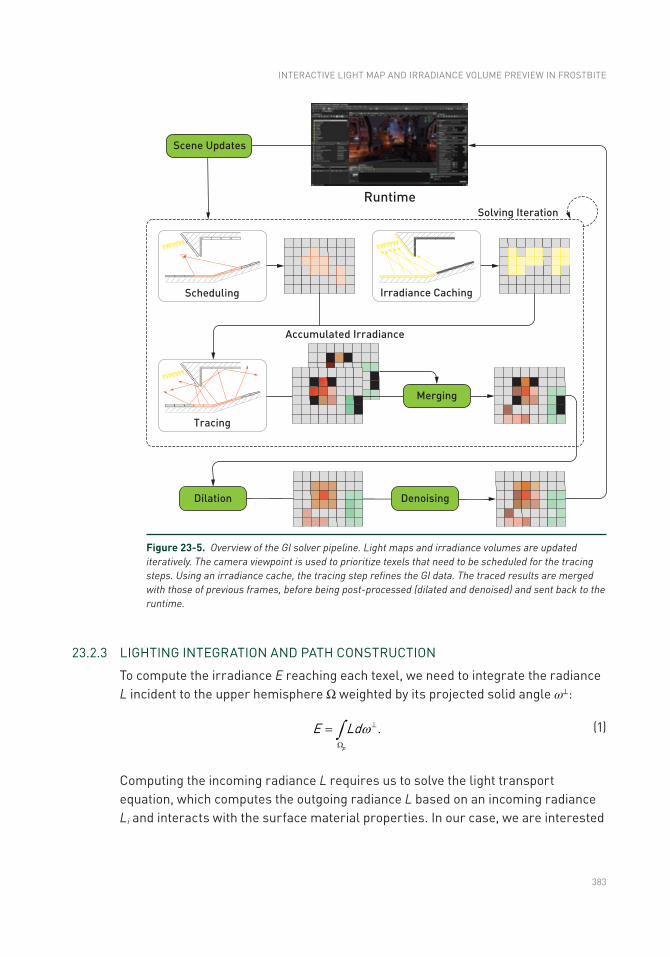
383
Figure 23-5. Overview of the GI solver pipeline. Light maps and irradiance volumes are updated iteratively. The camera viewpoint is used to prioritize texels that need to be scheduled for the tracing steps. Using an irradiance cache, the tracing step refines the GI data. The traced results are merged with those of previous frames, before being post-processed (dilated and denoised) and sent back to the runtime.
23.2.3 LIGHTING INTEGRATION AND PATH CONSTRUCTION
To compute the irradiance E reaching each texel, we need to integrate the radiance L incident to the upper hemisphere Ω weighted by its projected solid angle ω⊥:
p
E Ld .wò ^
W
=
(1)
Computing the incoming radiance L requires us to solve the light transport equation, which computes the outgoing radiance L based on an incoming radiance Li and interacts with the surface material properties. In our case, we are interested
INTERACTIVE LIGHT MAP AND IRRADIANCE VOLUME PREVIEW IN FROSTBITE
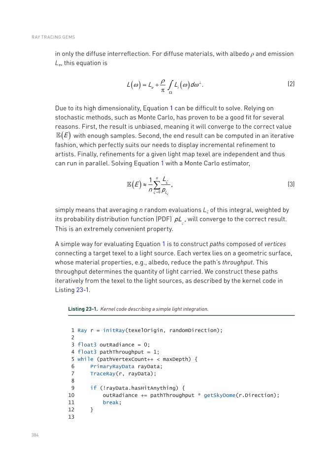
384
in only the diffuse interreflection. For diffuse materials, with albedo ρ and emission Le, this equation is
( ) ( )e iL L L d .rw w wò ^
W
= +p
(2)
Due to its high dimensionality, Equation 1 can be difficult to solve. Relying on stochastic methods, such as Monte Carlo, has proven to be a good fit for several reasons. First, the result is unbiased, meaning it will converge to the correct value ( )E with enough samples. Second, the end result can be computed in an iterative
fashion, which perfectly suits our needs to display incremental refinement to artists. Finally, refinements for a given light map texel are independent and thus can run in parallel. Solving Equation 1 with a Monte Carlo estimator,
( )
n
L
LE
n p0
1 ,z
z
z =
» å
(3)
simply means that averaging n random evaluations Lζ of this integral, weighted by its probability distribution function (PDF) pL
z, will converge to the correct result.
This is an extremely convenient property.
A simple way for evaluating Equation 1 is to construct paths composed of vertices connecting a target texel to a light source. Each vertex lies on a geometric surface, whose material properties, e.g., albedo, reduce the path’s throughput. This throughput determines the quantity of light carried. We construct these paths iteratively from the texel to the light sources, as described by the kernel code in Listing 23-1.
Listing 23-1. Kernel code describing a simple light integration.
1 Ray r = initRay(texelOrigin, randomDirection);
2
3 float3 outRadiance = 0;
4 float3 pathThroughput = 1;
5 while (pathVertexCount++ < maxDepth)
6 PrimaryRayData rayData;
7 TraceRay(r, rayData);
8
9 if (!rayData.hasHitAnything)
10 outRadiance += pathThroughput * getSkyDome(r.Direction);
11 break;
12
13
RAY TRACING GEMS
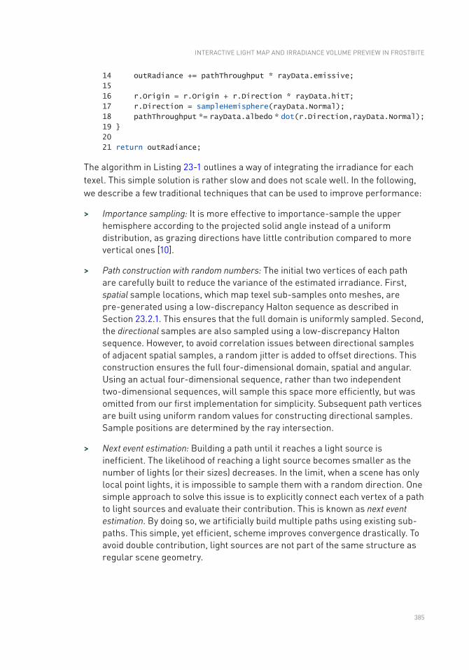
385
14 outRadiance += pathThroughput * rayData.emissive;
15
16 r.Origin = r.Origin + r.Direction * rayData.hitT;
17 r.Direction = sampleHemisphere(rayData.Normal);
18 pathThroughput *= rayData.albedo * dot(r.Direction,rayData.Normal);
19
20
21 return outRadiance;
The algorithm in Listing 23-1 outlines a way of integrating the irradiance for each texel. This simple solution is rather slow and does not scale well. In the following, we describe a few traditional techniques that can be used to improve performance:
> Importance sampling: It is more effective to importance-sample the upper hemisphere according to the projected solid angle instead of a uniform distribution, as grazing directions have little contribution compared to more vertical ones [10].
> Path construction with random numbers: The initial two vertices of each path are carefully built to reduce the variance of the estimated irradiance. First, spatial sample locations, which map texel sub- samples onto meshes, are pre-generated using a low-discrepancy Halton sequence as described in Section 23.2.1. This ensures that the full domain is uniformly sampled. Second, the directional samples are also sampled using a low-discrepancy Halton sequence. However, to avoid correlation issues between directional samples of adjacent spatial samples, a random jitter is added to offset directions. This construction ensures the full four-dimensional domain, spatial and angular. Using an actual four-dimensional sequence, rather than two independent two-dimensional sequences, will sample this space more efficiently, but was omitted from our first implementation for simplicity. Subsequent path vertices are built using uniform random values for constructing directional samples. Sample positions are determined by the ray intersection.
> Next event estimation: Building a path until it reaches a light source is inefficient. The likelihood of reaching a light source becomes smaller as the number of lights (or their sizes) decreases. In the limit, when a scene has only local point lights, it is impossible to sample them with a random direction. One simple approach to solve this issue is to explicitly connect each vertex of a path to light sources and evaluate their contribution. This is known as next event estimation. By doing so, we artificially build multiple paths using existing sub-paths. This simple, yet efficient, scheme improves convergence drastically. To avoid double contribution, light sources are not part of the same structure as regular scene geometry.
INTERACTIVE LIGHT MAP AND IRRADIANCE VOLUME PREVIEW IN FROSTBITE
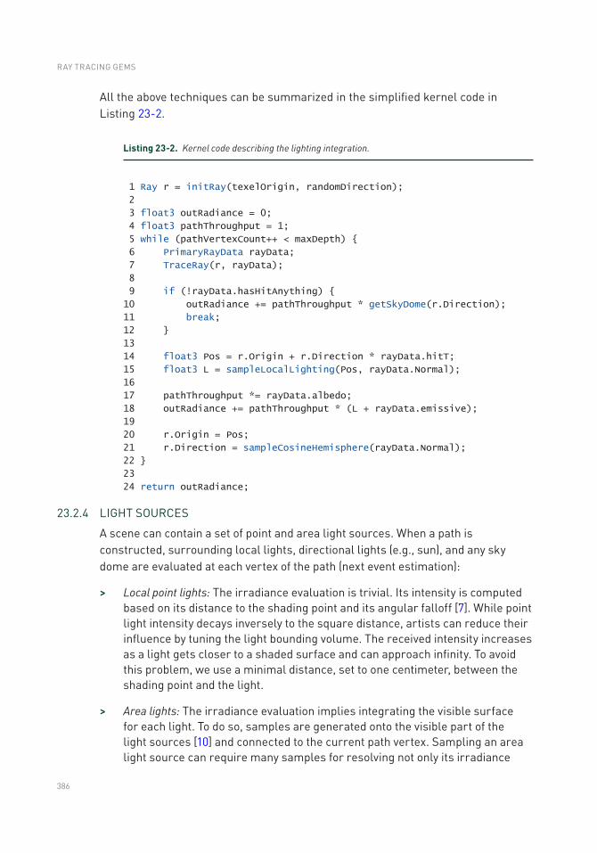
386
All the above techniques can be summarized in the simplified kernel code in Listing 23-2.
Listing 23-2. Kernel code describing the lighting integration.
1 Ray r = initRay(texelOrigin, randomDirection);
2
3 float3 outRadiance = 0;
4 float3 pathThroughput = 1;
5 while (pathVertexCount++ < maxDepth)
6 PrimaryRayData rayData;
7 TraceRay(r, rayData);
8
9 if (!rayData.hasHitAnything)
10 outRadiance += pathThroughput * getSkyDome(r.Direction);
11 break;
12
13
14 float3 Pos = r.Origin + r.Direction * rayData.hitT;
15 float3 L = sampleLocalLighting(Pos, rayData.Normal);
16
17 pathThroughput *= rayData.albedo;
18 outRadiance += pathThroughput * (L + rayData.emissive);
19
20 r.Origin = Pos;
21 r.Direction = sampleCosineHemisphere(rayData.Normal);
22
23
24 return outRadiance;
23.2.4 LIGHT SOURCES
A scene can contain a set of point and area light sources. When a path is constructed, surrounding local lights, directional lights (e.g., sun), and any sky dome are evaluated at each vertex of the path (next event estimation):
> Local point lights: The irradiance evaluation is trivial. Its intensity is computed based on its distance to the shading point and its angular falloff [7]. While point light intensity decays inversely to the square distance, artists can reduce their influence by tuning the light bounding volume. The received intensity increases as a light gets closer to a shaded surface and can approach infinity. To avoid this problem, we use a minimal distance, set to one centimeter, between the shading point and the light.
> Area lights: The irradiance evaluation implies integrating the visible surface for each light. To do so, samples are generated onto the visible part of the light sources [10] and connected to the current path vertex. Sampling an area light source can require many samples for resolving not only its irradiance
RAY TRACING GEMS
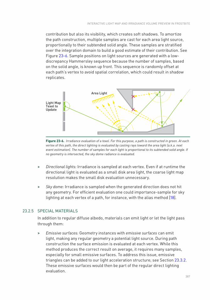
387
contribution but also its visibility, which creates soft shadows. To amortize the path construction, multiple samples are cast for each area light source, proportionally to their subtended solid angle. These samples are stratified over the integration domain to build a good estimate of their contribution. See Figure 23-6. Sample positions on light sources are generated with a low-discrepancy Hammersley sequence because the number of samples, based on the solid angle, is known up front. This sequence is randomly offset at each path’s vertex to avoid spatial correlation, which could result in shadow replicates.
> Directional lights: Irradiance is sampled at each vertex. Even if at runtime the directional light is evaluated as a small disk area light, the coarse light map resolution makes the small disk evaluation unnecessary.
> Sky dome: Irradiance is sampled when the generated direction does not hit any geometry. For efficient evaluation one could importance- sample for sky lighting at each vertex of a path, for instance, with the alias method [18].
23.2.5 SPECIAL MATERIALS
In addition to regular diffuse albedo, materials can emit light or let the light pass through them:
> Emissive surfaces: Geometry instances with emissive surfaces can emit light, making any regular geometry a potential light source. During path construction the surface emission is evaluated at each vertex. While this method produces the correct result on average, it requires many samples, especially for small emissive surfaces. To address this issue, emissive triangles can be added to our light acceleration structure; see Section 23.3.2. These emissive surfaces would then be part of the regular direct lighting evaluation.
Figure 23-6. Irradiance evaluation of a texel. For this purpose, a path is constructed in green. At each vertex of this path, the direct lighting is evaluated by casting rays toward the area light (a.k.a. next event estimation). The number of samples for each light is proportional to its subtended solid angle. If no geometry is intersected, the sky dome radiance is evaluated.
INTERACTIVE LIGHT MAP AND IRRADIANCE VOLUME PREVIEW IN FROSTBITE
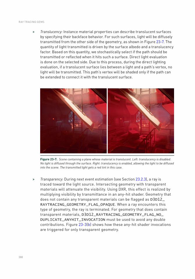
388
> Translucency: Instance material properties can describe translucent surfaces by specifying their backface behavior. For such surfaces, light will be diffusely transmitted from the other side of the geometry, as shown in Figure 23-7. The quantity of light transmitted is driven by the surface albedo and a translucency factor. Based on this quantity, we stochastically select if the path should be transmitted or reflected when it hits such a surface. Direct light evaluation is done on the selected side. Due to this process, during the direct lighting evaluation, if a translucent surface lies between a light and a path’s vertex, no light will be transmitted. This path’s vertex will be shaded only if the path can be extended to connect it with the translucent surface.
> Transparency: During next event estimation (see Section 23.2.3), a ray is traced toward the light source. Intersecting geometry with transparent materials will attenuate the visibility. Using DXR, this effect is realized by multiplying visibility by transmittance in an any- hit shader. Geometry that does not contain any transparent materials can be flagged as D3D12_RAYTRACING_GEOMETRY_FLAG_OPAQUE. When a ray encounters this type of geometry, the ray is terminated. For geometry that does contain transparent materials, D3D12_RAYTRACING_GEOMETRY_FLAG_NO_DUPLICATE_ANYHIT_INVOCATION must be used to avoid any double contributions. Figure 23-3(b) shows how these any-hit shader invocations are triggered for only transparent geometry.
Figure 23-7. Scene containing a plane whose material is translucent. Left: translucency is disabled. No light is diffused through the surface. Right: translucency is enabled, allowing the light to be diffused into the scene. The transmitted light gets a red tint in this case.
RAY TRACING GEMS
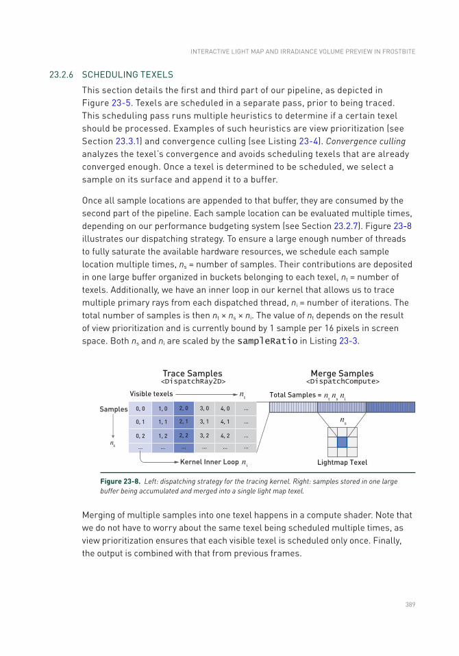
389
23.2.6 SCHEDULING TEXELS
This section details the first and third part of our pipeline, as depicted in Figure 23-5. Texels are scheduled in a separate pass, prior to being traced. This scheduling pass runs multiple heuristics to determine if a certain texel should be processed. Examples of such heuristics are view prioritization (see Section 23.3.1) and convergence culling (see Listing 23-4). Convergence culling analyzes the texel’s convergence and avoids scheduling texels that are already converged enough. Once a texel is determined to be scheduled, we select a sample on its surface and append it to a buffer.
Once all sample locations are appended to that buffer, they are consumed by the second part of the pipeline. Each sample location can be evaluated multiple times, depending on our performance budgeting system (see Section 23.2.7). Figure 23-8 illustrates our dispatching strategy. To ensure a large enough number of threads to fully saturate the available hardware resources, we schedule each sample location multiple times, ns = number of samples. Their contributions are deposited in one large buffer organized in buckets belonging to each texel, nt = number of texels. Additionally, we have an inner loop in our kernel that allows us to trace multiple primary rays from each dispatched thread, ni = number of iterations. The total number of samples is then nt × ns × ni. The value of nt depends on the result of view prioritization and is currently bound by 1 sample per 16 pixels in screen space. Both ns and ni are scaled by the sampleRatio in Listing 23-3.
Figure 23-8. Left: dispatching strategy for the tracing kernel. Right: samples stored in one large buffer being accumulated and merged into a single light map texel.
Merging of multiple samples into one texel happens in a compute shader. Note that we do not have to worry about the same texel being scheduled multiple times, as view prioritization ensures that each visible texel is scheduled only once. Finally, the output is combined with that from previous frames.
INTERACTIVE LIGHT MAP AND IRRADIANCE VOLUME PREVIEW IN FROSTBITE
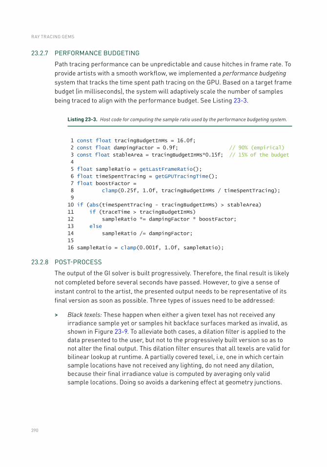
390
23.2.7 PERFORMANCE BUDGETING
Path tracing performance can be unpredictable and cause hitches in frame rate. To provide artists with a smooth workflow, we implemented a performance budgeting system that tracks the time spent path tracing on the GPU. Based on a target frame budget (in milliseconds), the system will adaptively scale the number of samples being traced to align with the performance budget. See Listing 23-3.
Listing 23-3. Host code for computing the sample ratio used by the performance budgeting system.
1 const float tracingBudgetInMs = 16.0f;
2 const float dampingFactor = 0.9f; // 90% (empirical)
3 const float stableArea = tracingBudgetInMs*0.15f; // 15% of the budget
4
5 float sampleRatio = getLastFrameRatio();
6 float timeSpentTracing = getGPUTracingTime();
7 float boostFactor =
8 clamp(0.25f, 1.0f, tracingBudgetInMs / timeSpentTracing);
9
10 if (abs(timeSpentTracing - tracingBudgetInMs) > stableArea)
11 if (traceTime > tracingBudgetInMs)
12 sampleRatio *= dampingFactor * boostFactor;
13 else
14 sampleRatio /= dampingFactor;
15
16 sampleRatio = clamp(0.001f, 1.0f, sampleRatio);
23.2.8 POST-PROCESS
The output of the GI solver is built progressively. Therefore, the final result is likely not completed before several seconds have passed. However, to give a sense of instant control to the artist, the presented output needs to be representative of its final version as soon as possible. Three types of issues need to be addressed:
> Black texels: These happen when either a given texel has not received any irradiance sample yet or samples hit backface surfaces marked as invalid, as shown in Figure 23-9. To alleviate both cases, a dilation filter is applied to the data presented to the user, but not to the progressively built version so as to not alter the final output. This dilation filter ensures that all texels are valid for bilinear lookup at runtime. A partially covered texel, i.e, one in which certain sample locations have not received any lighting, do not need any dilation, because their final irradiance value is computed by averaging only valid sample locations. Doing so avoids a darkening effect at geometry junctions.
RAY TRACING GEMS
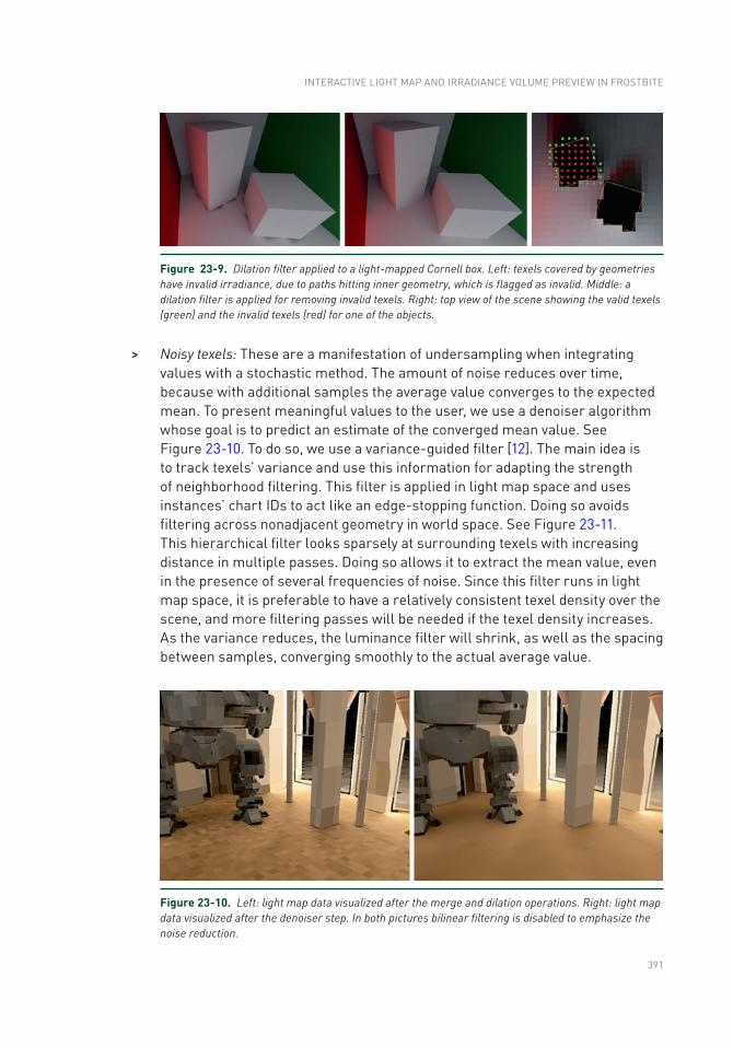
391
Figure 23-9. Dilation filter applied to a light-mapped Cornell box. Left: texels covered by geometries have invalid irradiance, due to paths hitting inner geometry, which is flagged as invalid. Middle: a dilation filter is applied for removing invalid texels. Right: top view of the scene showing the valid texels (green) and the invalid texels (red) for one of the objects.
> Noisy texels: These are a manifestation of undersampling when integrating values with a stochastic method. The amount of noise reduces over time, because with additional samples the average value converges to the expected mean. To present meaningful values to the user, we use a denoiser algorithm whose goal is to predict an estimate of the converged mean value. See Figure 23-10. To do so, we use a variance-guided filter [12]. The main idea is to track texels’ variance and use this information for adapting the strength of neighborhood filtering. This filter is applied in light map space and uses instances’ chart IDs to act like an edge-stopping function. Doing so avoids filtering across nonadjacent geometry in world space. See Figure 23- 11. This hierarchical filter looks sparsely at surrounding texels with increasing distance in multiple passes. Doing so allows it to extract the mean value, even in the presence of several frequencies of noise. Since this filter runs in light map space, it is preferable to have a relatively consistent texel density over the scene, and more filtering passes will be needed if the texel density increases. As the variance reduces, the luminance filter will shrink, as well as the spacing between samples, converging smoothly to the actual average value.
Figure 23-10. Left: light map data visualized after the merge and dilation operations. Right: light map data visualized after the denoiser step. In both pictures bilinear filtering is disabled to emphasize the noise reduction.
INTERACTIVE LIGHT MAP AND IRRADIANCE VOLUME PREVIEW IN FROSTBITE
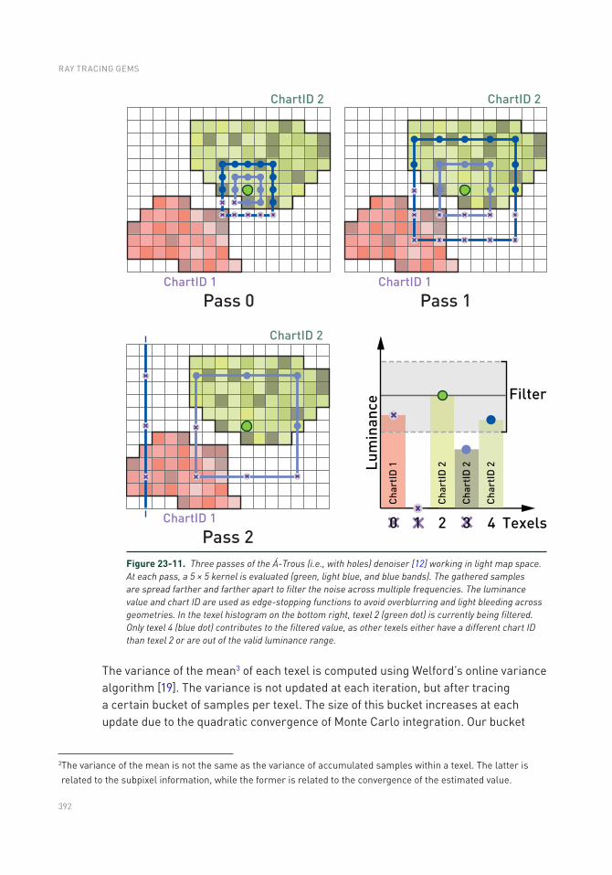
392
The variance of the mean3 of each texel is computed using Welford’s online variance algorithm [19]. The variance is not updated at each iteration, but after tracing a certain bucket of samples per texel. The size of this bucket increases at each update due to the quadratic convergence of Monte Carlo integration. Our bucket
3 The variance of the mean is not the same as the variance of accumulated samples within a texel. The latter is related to the subpixel information, while the former is related to the convergence of the estimated value.
Figure 23-11. Three passes of the Á-Trous (i.e., with holes) denoiser [12] working in light map space. At each pass, a 5 × 5 kernel is evaluated (green, light blue, and blue bands). The gathered samples are spread farther and farther apart to filter the noise across multiple frequencies. The luminance value and chart ID are used as edge-stopping functions to avoid overblurring and light bleeding across geometries. In the texel histogram on the bottom right, texel 2 (green dot) is currently being filtered. Only texel 4 (blue dot) contributes to the filtered value, as other texels either have a different chart ID than texel 2 or are out of the valid luminance range.
RAY TRACING GEMS
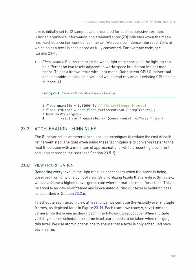
393
size is initially set to 12 samples and is doubled for each successive iteration. Using this variance information, the standard error [20] indicates when the mean has reached a certain confidence interval. We use a confidence interval of 95%, at which point a texel is considered as fully converged. For example code, see Listing 23-4.
> Chart seams: Seams can arise between light map charts, as the lighting can be different on two texels adjacent in world space but distant in light map space. This is a known issue with light maps. Our current GPU GI solver tool does not address this issue yet, and we instead rely on our existing CPU-based stitcher [4].
Listing 23-4. Kernel code describing variance tracking.
1 float quantile = 1.959964f; // 95% confidence interval
2 float stdError = sqrt(float(varianceOfMean / sampleCount));
3 bool hasConverged =
4 (stdError * quantile) <= (convergenceErrorThres * mean);
23.3 ACCELERATION TECHNIQUES
The GI solver relies on several acceleration techniques to reduce the cost of each refinement step. The goal when using these techniques is to converge faster to the final GI solution with a minimum of approximations, while presenting a coherent result on screen to the user (see Section 23.5.2).
23.3.1 VIEW PRIORITIZATION
Rendering every texel in the light map is unnecessary when the scene is being observed from only one point of view. By prioritizing texels that are directly in view, we can achieve a higher convergence rate where it matters most for artists. This is referred to as view prioritization and is evaluated during our texel scheduling pass, as described in Section 23.2.6.
To schedule each texel in view at least once, we compute the visibility over multiple frames, as depicted later in Figure 23-19. Each frame we trace nv rays from the camera into the scene as described in the following pseudocode. When multiple visibility queries schedule the same texel, care needs to be taken when merging this texel. We use atomic operations to ensure that a texel is only scheduled once each frame.
INTERACTIVE LIGHT MAP AND IRRADIANCE VOLUME PREVIEW IN FROSTBITE
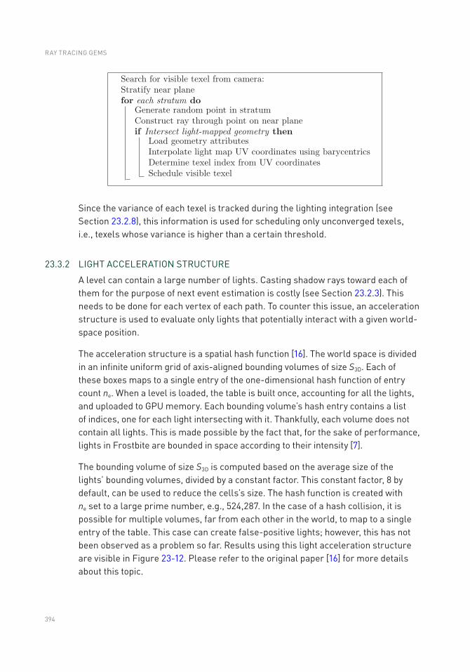
394
Since the variance of each texel is tracked during the lighting integration (see Section 23.2.8), this information is used for scheduling only unconverged texels, i.e., texels whose variance is higher than a certain threshold.
23.3.2 LIGHT ACCELERATION STRUCTURE
A level can contain a large number of lights. Casting shadow rays toward each of them for the purpose of next event estimation is costly (see Section 23.2.3). This needs to be done for each vertex of each path. To counter this issue, an acceleration structure is used to evaluate only lights that potentially interact with a given world-space position.
The acceleration structure is a spatial hash function [16]. The world space is divided in an infinite uniform grid of axis-aligned bounding volumes of size S3D. Each of these boxes maps to a single entry of the one-dimensional hash function of entry count ne. When a level is loaded, the table is built once, accounting for all the lights, and uploaded to GPU memory. Each bounding volume’s hash entry contains a list of indices, one for each light intersecting with it. Thankfully, each volume does not contain all lights. This is made possible by the fact that, for the sake of performance, lights in Frostbite are bounded in space according to their intensity [7].
The bounding volume of size S3D is computed based on the average size of the lights’ bounding volumes, divided by a constant factor. This constant factor, 8 by default, can be used to reduce the cells’s size. The hash function is created with ne set to a large prime number, e.g., 524,287. In the case of a hash collision, it is possible for multiple volumes, far from each other in the world, to map to a single entry of the table. This case can create false-positive lights; however, this has not been observed as a problem so far. Results using this light acceleration structure are visible in Figure 23-12. Please refer to the original paper [16] for more details about this topic.
RAY TRACING GEMS
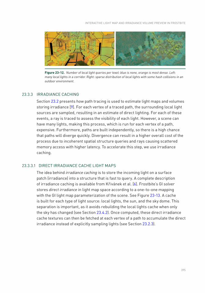
395
23.3.3 IRRADIANCE CACHING
Section 23.2 presents how path tracing is used to estimate light maps and volumes storing irradiance [9]. For each vertex of a traced path, the surrounding local light sources are sampled, resulting in an estimate of direct lighting. For each of these events, a ray is traced to assess the visibility of each light. However, a scene can have many lights, making this process, which is run for each vertex of a path, expensive. Furthermore, paths are built independently, so there is a high chance that paths will diverge quickly. Divergence can result in a higher overall cost of the process due to incoherent spatial structure queries and rays causing scattered memory access with higher latency. To accelerate this step, we use irradiance caching.
23.3.3.1 DIRECT IRRADIANCE CACHE LIGHT MAPS
The idea behind irradiance caching is to store the incoming light on a surface patch (irradiance) into a structure that is fast to query. A complete description of irradiance caching is available from Křivánek et al. [6]. Frostbite’s GI solver stores direct irradiance in light map space according to a one-to-one mapping with the GI light map parameterization of the scene. See Figure 23-13. A cache is built for each type of light source: local lights, the sun, and the sky dome. This separation is important, as it avoids rebuilding the local lights cache when only the sky has changed (see Section 23.4.2). Once computed, these direct irradiance cache textures can then be fetched at each vertex of a path to accumulate the direct irradiance instead of explicitly sampling lights (see Section 23.2.3).
Figure 23-12. Number of local light queries per texel: blue is none, orange is most dense. Left: many local lights in a corridor. Right: sparse distribution of local lights with some hash collisions in an outdoor environment.
INTERACTIVE LIGHT MAP AND IRRADIANCE VOLUME PREVIEW IN FROSTBITE
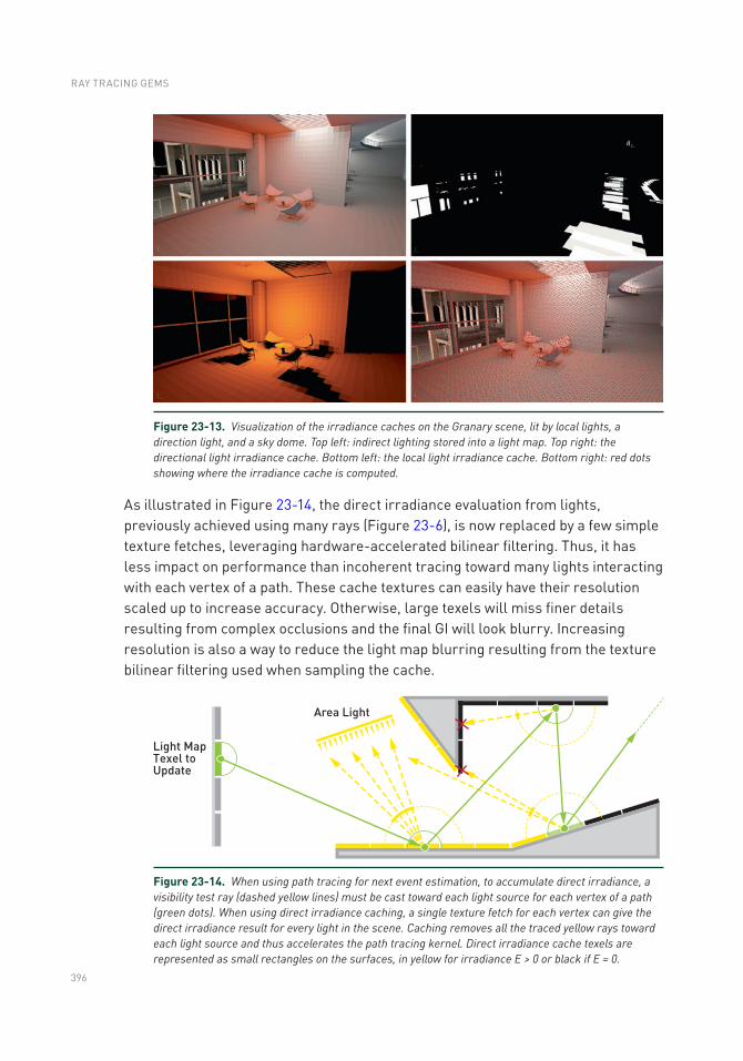
396
Figure 23-13. Visualization of the irradiance caches on the Granary scene, lit by local lights, a direction light, and a sky dome. Top left: indirect lighting stored into a light map. Top right: the directional light irradiance cache. Bottom left: the local light irradiance cache. Bottom right: red dots showing where the irradiance cache is computed.
As illustrated in Figure 23-14, the direct irradiance evaluation from lights, previously achieved using many rays (Figure 23-6), is now replaced by a few simple texture fetches, leveraging hardware-accelerated bilinear filtering. Thus, it has less impact on performance than incoherent tracing toward many lights interacting with each vertex of a path. These cache textures can easily have their resolution scaled up to increase accuracy. Otherwise, large texels will miss finer details resulting from complex occlusions and the final GI will look blurry. Increasing resolution is also a way to reduce the light map blurring resulting from the texture bilinear filtering used when sampling the cache.
Figure 23-14. When using path tracing for next event estimation, to accumulate direct irradiance, a visibility test ray (dashed yellow lines) must be cast toward each light source for each vertex of a path (green dots). When using direct irradiance caching, a single texture fetch for each vertex can give the direct irradiance result for every light in the scene. Caching removes all the traced yellow rays toward each light source and thus accelerates the path tracing kernel. Direct irradiance cache texels are represented as small rectangles on the surfaces, in yellow for irradiance E > 0 or black if E = 0.
RAY TRACING GEMS
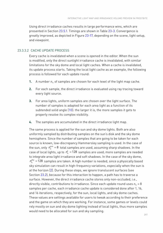
397
Using direct irradiance caches results in large performance wins, which are presented in Section 23.5.1. Timings are shown in Table 23-3. Convergence is greatly improved, as depicted in Figure 23-17, depending on the scene, light setup, and viewpoint.
23.3.3.2 CACHE UPDATE PROCESS
Every cache is invalidated when a scene is opened in the editor. When the sun is modified, only the direct sunlight irradiance cache is invalidated, with similar limitations for the sky dome and local light caches. When a cache is invalidated, its update process starts. Taking the local light cache as an example, the following process is followed for each update round:
1. A number nic of samples are chosen for each texel of the light map cache.
2. For each sample, the direct irradiance is evaluated using ray tracing toward every light source.
3. For area lights, uniform samples are chosen over the light surface. The number of samples is adapted for each area light as a function of its subtended solid angle [10]: the larger it is, the more samples it gets to properly resolve its complex visibility.
4. The samples are accumulated in the direct irradiance light map.
The same process is applied for the sun and sky dome lights. Both are also uniformly sampled by distributing samples on the sun’s disk and the sky dome hemisphere. Since the number of samples that are going to be taken for each source is known, low- discrepancy Hammersley sampling is used. In the case of the sun, only nsun
ic 8= total samples are used, assuming sharp shadows. In the case of local lights, up to nL
ic 128= samples are used; more samples are needed to integrate area light irradiance and soft shadows. In the case of the sky dome, nsky
ic 128= samples are taken. A high number is needed, since a physically based sky simulation can result in high-frequency variations, especially when the sun is at the horizon [2]. During these steps, we ignore translucent surfaces (see Section 23.2), because for this interaction to happen, a path has to traverse a surface. However, the direct irradiance cache stores only non-occluded, i.e., directly visible, contributions to irradiance. Since each update round uses nic = 8 samples per cache, each irradiance cache update is considered done after 1, 16, and 16 iterations, respectively, for the sun, local lights, and sky dome caches. These values are settings available for users to tweak according to their preference and the game on which they are working. For instance, some games or levels could rely mostly on sun and sky dome lighting instead of local lights, thus more samples would need to be allocated for sun and sky sampling.
INTERACTIVE LIGHT MAP AND IRRADIANCE VOLUME PREVIEW IN FROSTBITE
398
23.3.3.3 FUTURE IMPROVEMENTS
Indirect irradiance cache In addition to direct light caching, accumulated indirect irradiance can be used to shorten path sampling. As described in Section 23.2.8, each texel convergence is tracked. When a texel is fully converged, its value can be used as an estimate of incident indirect lighting. By doing so, the path can end there, reducing the amount of computation.
Emissive surfaces As of today, emissive surfaces are not taken into account in any of the direct irradiance caches. In Section 23.2.4, we mention that such surfaces could be converted to triangle area lights. Such area lights could be sampled to populate a direct irradiance cache light map dedicated to emissive surfaces. This cache would then only be updated when a mesh is moved or a material property affecting emitted surface radiance is modified by an artist.
23.4 LIVE UPDATE
23.4.1 LIGHTING ARTIST WORKFLOW IN PRODUCTION
Frostbite-based game teams have dedicated artists responsible for designing the lighting and thereby setting the mood of a scene. There are several editing operations that lighting artists use to accomplish this. The most common include placing lights sources, adjusting them, moving objects, and changing their materials. Other operations include modifying light map resolution for individual objects and switching objects from being lit by a light map or by irradiance volumes. These two operations mainly aim to adjust memory usage to fit within a certain light map budget.
As stated in Section 23.1, the offline Frostbite GI solver uses CPU-based ray tracing. Historically, getting feedback on the work performed in the game editor with regard to global illumination takes minutes to hours when using a CPU-based solver. The transition to GPU-based ray tracing allows the time range for this process to become seconds to minutes. The raw performance when taking a scene from nothing to one with reasonable global illumination is important in this context. The general acceleration techniques used are described in Section 23.3. The next section focuses on optimizations made possible when dealing with a specific modification done to the scene by the artist.
23.4.2 SCENE MANIPULATION AND DATA INVALIDATION
For a scene, light maps, irradiance volumes, and irradiance caches are considered states, which are updated after each iteration of the GI preview. When a light, mesh, or material is updated, the current GI states become invalid. However, it is
RAY TRACING GEMS
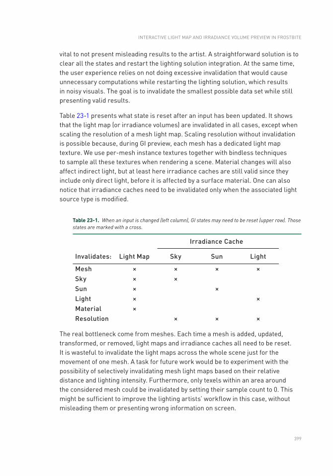
399
vital to not present misleading results to the artist. A straightforward solution is to clear all the states and restart the lighting solution integration. At the same time, the user experience relies on not doing excessive invalidation that would cause unnecessary computations while restarting the lighting solution, which results in noisy visuals. The goal is to invalidate the smallest possible data set while still presenting valid results.
Table 23-1 presents what state is reset after an input has been updated. It shows that the light map (or irradiance volumes) are invalidated in all cases, except when scaling the resolution of a mesh light map. Scaling resolution without invalidation is possible because, during GI preview, each mesh has a dedicated light map texture. We use per- mesh instance textures together with bindless techniques to sample all these textures when rendering a scene. Material changes will also affect indirect light, but at least here irradiance caches are still valid since they include only direct light, before it is affected by a surface material. One can also notice that irradiance caches need to be invalidated only when the associated light source type is modified.
Table 23-1. When an input is changed (left column), GI states may need to be reset (upper row). Those states are marked with a cross.
The real bottleneck come from meshes. Each time a mesh is added, updated, transformed, or removed, light maps and irradiance caches all need to be reset. It is wasteful to invalidate the light maps across the whole scene just for the movement of one mesh. A task for future work would be to experiment with the possibility of selectively invalidating mesh light maps based on their relative distance and lighting intensity. Furthermore, only texels within an area around the considered mesh could be invalidated by setting their sample count to 0. This might be sufficient to improve the lighting artists’ workflow in this case, without misleading them or presenting wrong information on screen.
INTERACTIVE LIGHT MAP AND IRRADIANCE VOLUME PREVIEW IN FROSTBITE
400
23.5 PERFORMANCE AND HARDWARE
23.5.1 METHOD
In recent ray tracing–related work, the performance metrics used are often technically oriented, such as giga-rays per second or a simple frames per second. In this project, the focus instead has been on the lighting artist’s experience, and therefore our methods to assess performance reflect this. Performance manifests itself to the artist as refresh rate and convergence rate, i.e., how often and to what quality lighting conditions are presented to the user.
The quality of the GI solver’s progressive output is assessed using a perceptual image difference measure, and the error is tracked over time. The L1 metric was simple and sufficient for our use case [13]. The L1 metric is applied to the results of the GI solver, i.e., light maps or irradiance volumes. Only texels in view that affect the viewed result are part of the calculation. A texel is considered significant if it is scheduled in at least 1% of all the update iterations. To limit the number of independent variables, the refresh rate has been fixed to 33 milliseconds in these tests.
To be able to calculate a perceptual image difference, an image representing ground truth is needed. It is computed using the base version of our GI solver pipeline, without optimizations or simplifications and without using time restrictions. Convergence is computed continuously. When each texel has reached a certain threshold of convergence (for details see Section 23.2), the resulting light maps and irradiance volumes are stored as a reference.
A specific acceleration technique can be assessed by adding it to the GI solver. The test starts by invalidating the state, depending on what user operation we want to simulate (as described in Section 23.4). As the process continues, after each iteration the results are compared with the reference and the metric gets applied.
The metric results in an error, or distance, from the ground truth. The error is logged and used to graph how it changes over time, and it is compared to a GI solver that does not include the acceleration technique.
23.5.2 RESULTS
Two different scenes with one viewpoint for each of them are used to measure performance. They are meant to represent typical use cases for our lighting artists. The first is an indoor scene mainly lit by local lights (Granary by Night) and the second is a large-scale outdoor scene from a production game (Zen Peak level from Plants vs. Zombies Garden Warfare 2). To give a sense of the complexity of each scene’s view, both are presented visually in Figure 23-15 and their statistics are presented in Table 23-2. Apart from what is shown in the table,
RAY TRACING GEMS
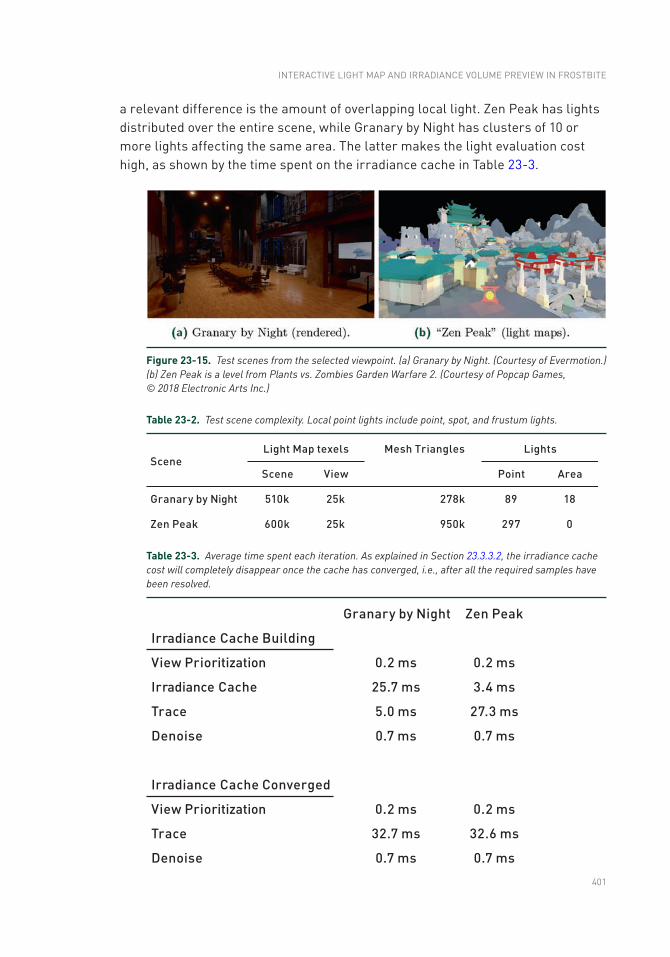
401
a relevant difference is the amount of overlapping local light. Zen Peak has lights distributed over the entire scene, while Granary by Night has clusters of 10 or more lights affecting the same area. The latter makes the light evaluation cost high, as shown by the time spent on the irradiance cache in Table 23-3.
Figure 23-15. Test scenes from the selected viewpoint. (a) Granary by Night. (Courtesy of Evermotion.) (b) Zen Peak is a level from Plants vs. Zombies Garden Warfare 2. (Courtesy of Popcap Games, © 2018 Electronic Arts Inc.)
Table 23-2. Test scene complexity. Local point lights include point, spot, and frustum lights.
Table 23-3. Average time spent each iteration. As explained in Section 23.3.3.2, the irradiance cache cost will completely disappear once the cache has converged, i.e., after all the required samples have been resolved.
INTERACTIVE LIGHT MAP AND IRRADIANCE VOLUME PREVIEW IN FROSTBITE
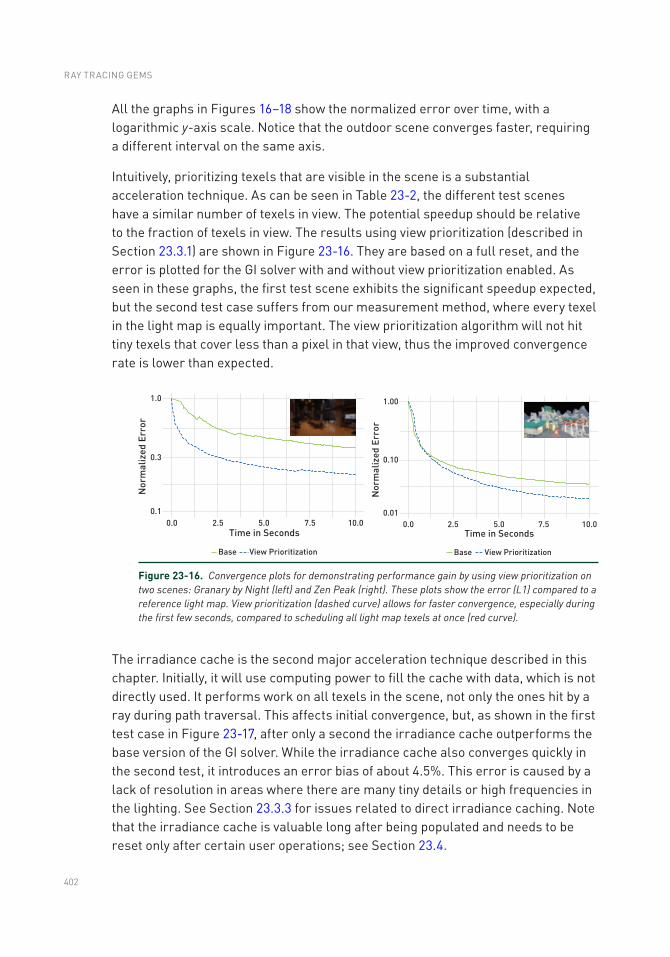
402
All the graphs in Figures 16–18 show the normalized error over time, with a logarithmic y-axis scale. Notice that the outdoor scene converges faster, requiring a different interval on the same axis.
Intuitively, prioritizing texels that are visible in the scene is a substantial acceleration technique. As can be seen in Table 23-2, the different test scenes have a similar number of texels in view. The potential speedup should be relative to the fraction of texels in view. The results using view prioritization (described in Section 23.3.1) are shown in Figure 23-16. They are based on a full reset, and the error is plotted for the GI solver with and without view prioritization enabled. As seen in these graphs, the first test scene exhibits the significant speedup expected, but the second test case suffers from our measurement method, where every texel in the light map is equally important. The view prioritization algorithm will not hit tiny texels that cover less than a pixel in that view, thus the improved convergence rate is lower than expected.
The irradiance cache is the second major acceleration technique described in this chapter. Initially, it will use computing power to fill the cache with data, which is not directly used. It performs work on all texels in the scene, not only the ones hit by a ray during path traversal. This affects initial convergence, but, as shown in the first test case in Figure 23-17, after only a second the irradiance cache outperforms the base version of the GI solver. While the irradiance cache also converges quickly in the second test, it introduces an error bias of about 4.5%. This error is caused by a lack of resolution in areas where there are many tiny details or high frequencies in the lighting. See Section 23.3.3 for issues related to direct irradiance caching. Note that the irradiance cache is valuable long after being populated and needs to be reset only after certain user operations; see Section 23.4.
Figure 23-16. Convergence plots for demonstrating performance gain by using view prioritization on two scenes: Granary by Night (left) and Zen Peak (right). These plots show the error (L1) compared to a reference light map. View prioritization (dashed curve) allows for faster convergence, especially during the first few seconds, compared to scheduling all light map texels at once (red curve).
RAY TRACING GEMS
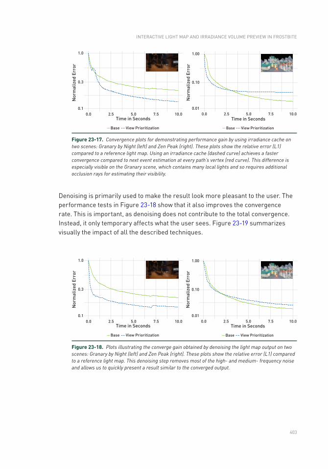
403
Denoising is primarily used to make the result look more pleasant to the user. The performance tests in Figure 23-18 show that it also improves the convergence rate. This is important, as denoising does not contribute to the total convergence. Instead, it only temporary affects what the user sees. Figure 23-19 summarizes visually the impact of all the described techniques.
Figure 23-17. Convergence plots for demonstrating performance gain by using irradiance cache on two scenes: Granary by Night (left) and Zen Peak (right). These plots show the relative error (L1) compared to a reference light map. Using an irradiance cache (dashed curve) achieves a faster convergence compared to next event estimation at every path’s vertex (red curve). This difference is especially visible on the Granary scene, which contains many local lights and so requires additional occlusion rays for estimating their visibility.
Figure 23-18. Plots illustrating the converge gain obtained by denoising the light map output on two scenes: Granary by Night (left) and Zen Peak (right). These plots show the relative error (L1) compared to a reference light map. This denoising step removes most of the high- and medium- frequency noise and allows us to quickly present a result similar to the converged output.
INTERACTIVE LIGHT MAP AND IRRADIANCE VOLUME PREVIEW IN FROSTBITE
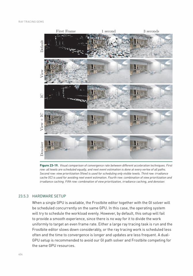
404
Figure 23-19. Visual comparison of convergence rate between different acceleration techniques. First row: all texels are scheduled equally, and next event estimation is done at every vertex of all paths. Second row: view prioritization (View) is used for scheduling only visible texels. Third row: irradiance cache (IC) is used for avoiding next event estimation. Fourth row: combination of view prioritization and irradiance caching. Fifth row: combination of view prioritization, irradiance caching, and denoiser.
23.5.3 HARDWARE SETUP
When a single GPU is available, the Frostbite editor together with the GI solver will be scheduled concurrently on the same GPU. In this case, the operating system will try to schedule the workload evenly. However, by default, this setup will fail to provide a smooth experience, since there is no way for it to divide the work uniformly to target an even frame rate. Either a large ray tracing task is run and the Frostbite editor slows down considerably, or the ray tracing work is scheduled less often and the time to convergence is longer and updates are less frequent. A dual-GPU setup is recommended to avoid our GI path solver and Frostbite competing for the same GPU resources.
RAY TRACING GEMS
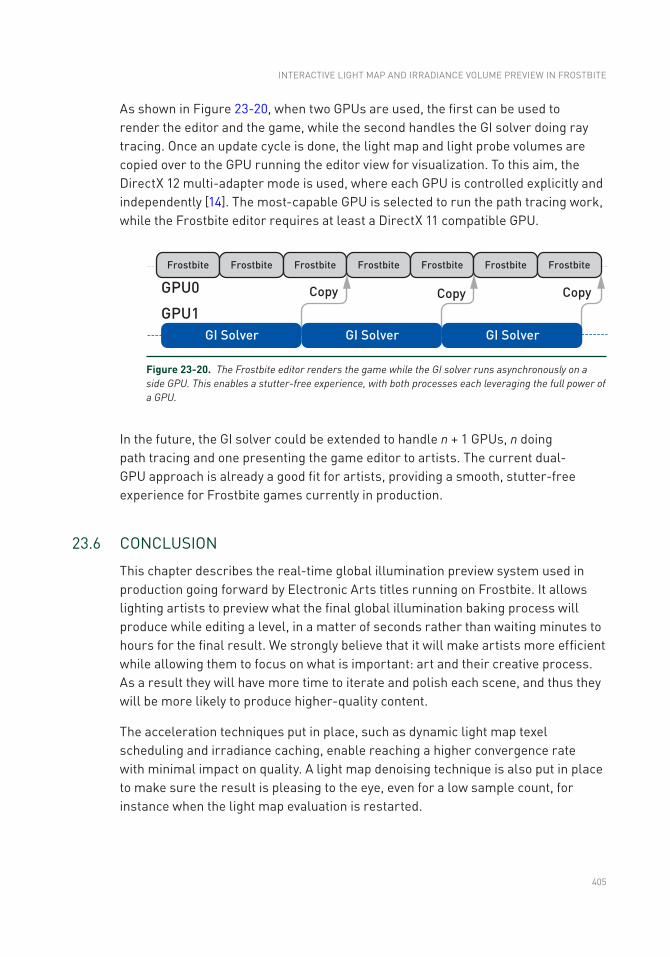
405
As shown in Figure 23-20, when two GPUs are used, the first can be used to render the editor and the game, while the second handles the GI solver doing ray tracing. Once an update cycle is done, the light map and light probe volumes are copied over to the GPU running the editor view for visualization. To this aim, the DirectX 12 multi-adapter mode is used, where each GPU is controlled explicitly and independently [14]. The most- capable GPU is selected to run the path tracing work, while the Frostbite editor requires at least a DirectX 11 compatible GPU.
In the future, the GI solver could be extended to handle n + 1 GPUs, n doing path tracing and one presenting the game editor to artists. The current dual-GPU approach is already a good fit for artists, providing a smooth, stutter-free experience for Frostbite games currently in production.
23.6 CONCLUSION
This chapter describes the real-time global illumination preview system used in production going forward by Electronic Arts titles running on Frostbite. It allows lighting artists to preview what the final global illumination baking process will produce while editing a level, in a matter of seconds rather than waiting minutes to hours for the final result. We strongly believe that it will make artists more efficient while allowing them to focus on what is important: art and their creative process. As a result they will have more time to iterate and polish each scene, and thus they will be more likely to produce higher-quality content.
The acceleration techniques put in place, such as dynamic light map texel scheduling and irradiance caching, enable reaching a higher convergence rate with minimal impact on quality. A light map denoising technique is also put in place to make sure the result is pleasing to the eye, even for a low sample count, for instance when the light map evaluation is restarted.
Figure 23-20. The Frostbite editor renders the game while the GI solver runs asynchronously on a side GPU. This enables a stutter-free experience, with both processes each leveraging the full power of a GPU.
INTERACTIVE LIGHT MAP AND IRRADIANCE VOLUME PREVIEW IN FROSTBITE
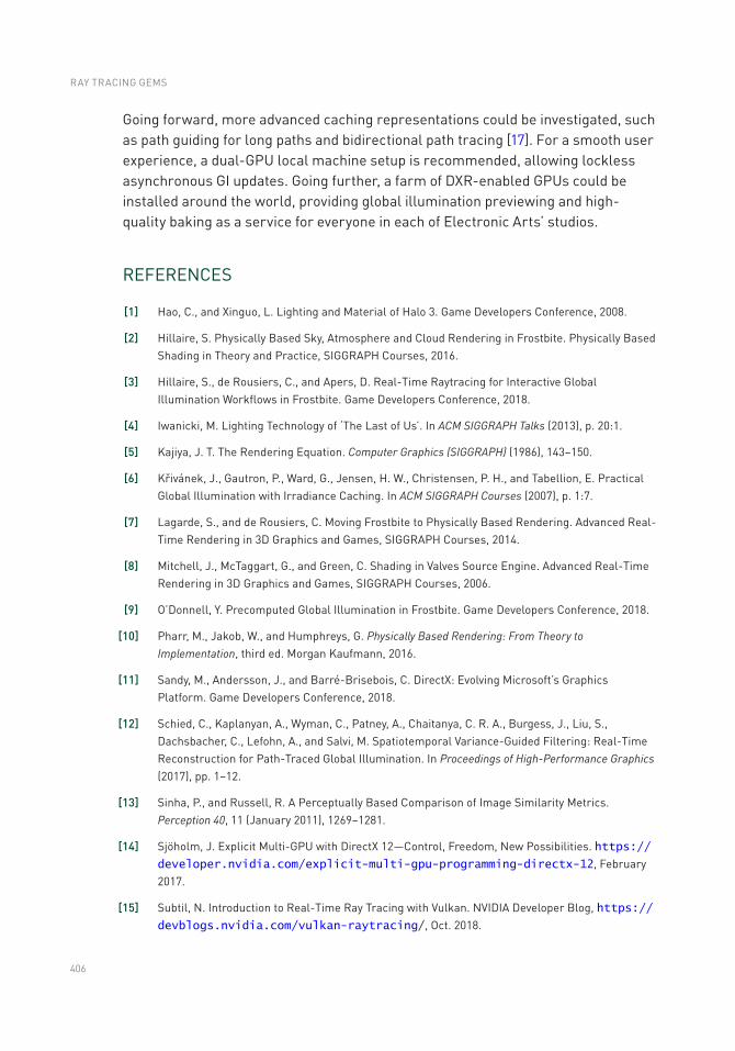
406
Going forward, more advanced caching representations could be investigated, such as path guiding for long paths and bidirectional path tracing [17]. For a smooth user experience, a dual-GPU local machine setup is recommended, allowing lockless asynchronous GI updates. Going further, a farm of DXR-enabled GPUs could be installed around the world, providing global illumination previewing and high-quality baking as a service for everyone in each of Electronic Arts’ studios.
REFERENCES
[1] Hao, C., and Xinguo, L. Lighting and Material of Halo 3. Game Developers Conference, 2008.
[2] Hillaire, S. Physically Based Sky, Atmosphere and Cloud Rendering in Frostbite. Physically Based Shading in Theory and Practice, SIGGRAPH Courses, 2016.
[3] Hillaire, S., de Rousiers, C., and Apers, D. Real-Time Raytracing for Interactive Global Illumination Workflows in Frostbite. Game Developers Conference, 2018.
[4] Iwanicki, M. Lighting Technology of ‘The Last of Us’. In ACM SIGGRAPH Talks (2013), p. 20:1.
[5] Kajiya, J. T. The Rendering Equation. Computer Graphics (SIGGRAPH) (1986), 143–150.
[6] Křivánek, J., Gautron, P., Ward, G., Jensen, H. W., Christensen, P. H., and Tabellion, E. Practical Global Illumination with Irradiance Caching. In ACM SIGGRAPH Courses (2007), p. 1:7.
[7] Lagarde, S., and de Rousiers, C. Moving Frostbite to Physically Based Rendering. Advanced Real-Time Rendering in 3D Graphics and Games, SIGGRAPH Courses, 2014.
[8] Mitchell, J., McTaggart, G., and Green, C. Shading in Valves Source Engine. Advanced Real-Time Rendering in 3D Graphics and Games, SIGGRAPH Courses, 2006.
[9] O’Donnell, Y. Precomputed Global Illumination in Frostbite. Game Developers Conference, 2018.
[10] Pharr, M., Jakob, W., and Humphreys, G. Physically Based Rendering: From Theory to Implementation, third ed. Morgan Kaufmann, 2016.
[11] Sandy, M., Andersson, J., and Barré-Brisebois, C. DirectX: Evolving Microsoft’s Graphics Platform. Game Developers Conference, 2018.
[12] Schied, C., Kaplanyan, A., Wyman, C., Patney, A., Chaitanya, C. R. A., Burgess, J., Liu, S., Dachsbacher, C., Lefohn, A., and Salvi, M. Spatiotemporal Variance- Guided Filtering: Real-Time Reconstruction for Path-Traced Global Illumination. In Proceedings of High-Performance Graphics (2017), pp. 1–12.
[13] Sinha, P., and Russell, R. A Perceptually Based Comparison of Image Similarity Metrics. Perception 40, 11 (January 2011), 1269–1281.
[14] Sjöholm, J. Explicit Multi-GPU with DirectX 12—Control, Freedom, New Possibilities. https://developer.nvidia.com/explicit-multi-gpu-programming-directx-12, February 2017.
[15] Subtil, N. Introduction to Real-Time Ray Tracing with Vulkan. NVIDIA Developer Blog, https://devblogs.nvidia.com/vulkan-raytracing/, Oct. 2018.
RAY TRACING GEMS

407
[16] Teschner, M., Heidelberger, B., Müller, M., Pomeranets, D., and Markus, G. Optimized Spatial Hashing for Collision Detection of Deformable Objects. In Proceedings of Vision, Modeling, Visualization Conference (2003), pp. 47–54.
[17] Vorba, J., Karlik, O., Šik, M., Ritschel, T., and Křivánek, J. On-line Learning of Parametric Mixture Models for Light Transport Simulation. ACM Transactions on Graphics 33, 4 (July 2014), 1–11.
[18] Walker, A.J. New Fast Method for Generating Discrete Random Numbers with Arbitrary Frequency Distributions. Electronics Letters 10, 8 (February 1974), 127–128.
[19] Wikipedia. Online Variance Calculation Algorithm (Knuth/Welford). Accessed 2018-12-10.
[20] Wikipedia. Standard Error. Accessed 2018-12-10.
Open Access This chapter is licensed under the terms of the Creative Commons Attribution-NonCommercial-NoDerivatives 4.0 International License (http://creativecommons.org/licenses/by-nc-nd/4.0/), which permits any noncommercial use, sharing, distribution and
reproduction in any medium or format, as long as you give appropriate credit to the original author(s) and the source, provide a link to the Creative Commons license and indicate if you modified the licensed material. You do not have permission under this license to share adapted material derived from this chapter or parts of it.
The images or other third party material in this chapter are included in the chapter's Creative Commons license, unless indicated otherwise in a credit line to the material. If material is not included in the chapter's Creative Commons license and your intended use is not permitted by statutory regulation or exceeds the permitted use, you will need to obtain permission directly from the copyright holder.
INTERACTIVE LIGHT MAP AND IRRADIANCE VOLUME PREVIEW IN FROSTBITE
409© NVIDIA 2019 E. Haines, T. Akenine-Möller (eds.), Ray Tracing Gems, https://doi.org/10.1007/978-1-4842-4427-2_24
CHAPTER 24
Real-Time Global Illumination with Photon MappingNiklas Smal and Maksim Aizenshtein UL Benchmarks
ABSTRACT
Indirect lighting, also known as global illumination, is a crucial effect in photorealistic images. While there are a number of effective global illumination techniques based on precomputation that work well with static scenes, including global illumination for scenes with dynamic lighting and dynamic geometry remains a challenging problem. In this chapter, we describe a real-time global illumination algorithm based on photon mapping that evaluates several bounces of indirect lighting without any precomputed data in scenes with both dynamic lighting and fully dynamic geometry. We explain both the pre- and post-processing steps required to achieve dynamic high-quality illumination within the limits of a real-time frame budget.
24.1 INTRODUCTION
As the scope of what is possible with real-time graphics has grown with the advancing capabilities of graphics hardware, scenes have become increasingly complex and dynamic. However, most of the current real-time global illumination algorithms (e.g., light maps and light probes) do not work well with moving lights and geometry due to these methods’ dependence on precomputed data.
In this chapter, we describe an approach based on an implementation of photon mapping [7], a Monte Carlo method that approximates lighting by first tracing paths of light-carrying photons in the scene to create a data structure that represents the indirect illumination and then using that structure to estimate indirect light at points being shaded. See Figure 24-1. Photon mapping has a number of useful properties, including that it is compatible with precomputed global illumination, provides a result with similar quality to current static techniques, can easily trade off quality and computation time, and requires no significant artist work. Our implementation of photon mapping is based on DirectX Raytracing (DXR) and gives high-quality global illumination with dynamic scenes. The overall structure of our approach is shown in Figure 24-2.
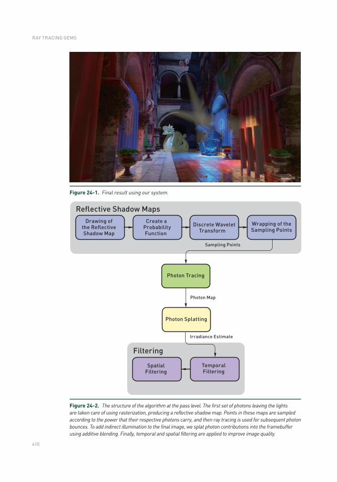
410
Figure 24-1. Final result using our system.
Figure 24-2. The structure of the algorithm at the pass level. The first set of photons leaving the lights are taken care of using rasterization, producing a reflective shadow map. Points in these maps are sampled according to the power that their respective photons carry, and then ray tracing is used for subsequent photon bounces. To add indirect illumination to the final image, we splat photon contributions into the framebuffer using additive blending. Finally, temporal and spatial filtering are applied to improve image quality.
RAY TRACING GEMS
411
Adapting photon mapping to real-time rendering on the GPU requires addressing a number of challenges. One is how to find nearby photons at points shaded in the scene so the photons can contribute indirect illumination to these locations. We found that an approach based on splatting, where each photon is rasterized into the image based on its contribution’s extent, works well and is straightforward to implement.
Another challenge is that traditional photon mapping algorithms may not be able to reach the desired illumination quality within the computational constraints of real-time rendering. Therefore, we optimized the generation of photons using reflective shadow maps (RSMs) [2] to avoid tracing the first bounce of a ray from a light, replacing that step with rasterization. We are then able to apply importance sampling to the RSMs, choosing locations with high contributions more often to generate subsequent photon paths.
Finally, as is always the case when applying Monte Carlo techniques to real-time rendering, effective filtering is crucial to remove image artifacts due to low sample counts. To mitigate noise, we use temporal accumulation with an exponentially moving average and apply an edge-aware spatial filter.
24.2 PHOTON TRACING
While general ray tracing is necessary for following the paths of photons that have reflected from surfaces, it is possible to take advantage of the fact that all the photons leaving a single point light source have a common origin. In our implementation, the first segment of each photon path is handled via rasterization. For each emitter, we generate a reflective shadow map [2, 3], which is effectively a G-buffer of uniform samples of visible surfaces as seen from a light, where each pixel also stores the incident illumination. This basic approach was first introduced by McGuire and Luebke [10] nearly a decade ago, though they traced rays on the CPU at much lower performance and thus also had to transfer a significant amount of data between the CPU and the GPU—all of this fortunately no longer necessary with DXR.
After the initial intersection points are found with rasterization, photon paths continue by sampling the surface’s BRDF and tracing rays. Photons are stored at all subsequent intersection points, to be used for reconstructing the illumination, as will be described in Section 24.3.
REAL-TIME GLOBAL ILLUMINATION WITH PHOTON MAPPING
412
24.2.1 RSM-BASED FIRST BOUNCE
We start by selecting a total number of photons to emit from all light sources and then allocate these to lights proportional to each light’s intensity. Hence, all photons initially carry roughly the same power. The RSM must contain all surface properties needed to generate rays for the initial bounce of the photons.
We choose to implement RSM generation as a separate pass that is executed after generating a traditional shadow map. Doing so allows us to make the resolution of the RSM map independent from the shadow map and keep its size constant, avoiding the need to allocate RSMs during runtime. As an optimization, it is possible to use the regular shadow map for depth culling. Without matching resolutions, this will give incorrect results for some pixels, but in our testing, we have not found it to cause visible artifacts.
After the RSMs are generated, we generate an importance map for sampling starting points for the first bounce where each RSM pixel is first given a weight based on the luminance of the product of the emitted power carried by the photon, including artist- controlled parameters such as directional falloff and the surface albedo. This weight value is directly related to the amount of power carried by photons that leave the surface.
This importance map is not normalized, which would be required for most sampling techniques. Rather than normalizing the map and generating sampling distributions, we instead apply a hierarchical sampling algorithm based on wavelet importance sampling, introduced by Clarberg et al. [1].
Wavelet importance sampling is a two-step algorithm. First, we apply the discrete Haar wavelet transform to the probability map, effectively generating a pyramid representation of the image. Second, we reconstruct the signal for each sample location in a low-discrepancy sequence and warp the sampling positions based on the scaling coefficient of each iteration in a wavelet transformation. This warping scheme is illustrated in Figure 24-3. See also Chapter 16, “Sampling Transformations Zoo,” for more information about it.
RAY TRACING GEMS
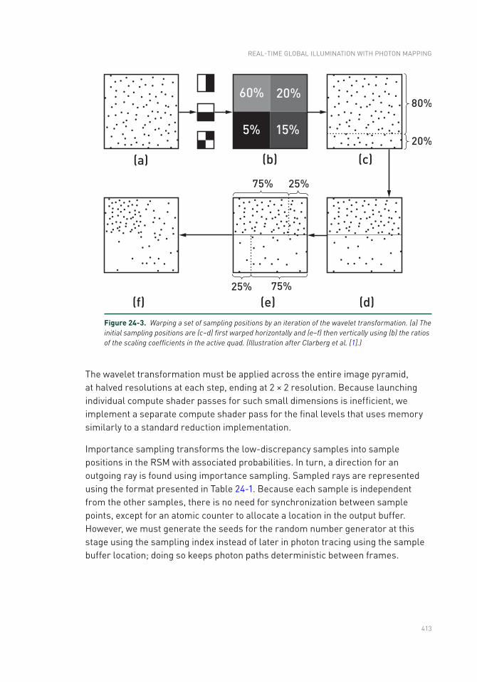
413
The wavelet transformation must be applied across the entire image pyramid, at halved resolutions at each step, ending at 2 × 2 resolution. Because launching individual compute shader passes for such small dimensions is inefficient, we implement a separate compute shader pass for the final levels that uses memory similarly to a standard reduction implementation.
Importance sampling transforms the low-discrepancy samples into sample positions in the RSM with associated probabilities. In turn, a direction for an outgoing ray is found using importance sampling. Sampled rays are represented using the format presented in Table 24-1. Because each sample is independent from the other samples, there is no need for synchronization between sample points, except for an atomic counter to allocate a location in the output buffer. However, we must generate the seeds for the random number generator at this stage using the sampling index instead of later in photon tracing using the sample buffer location; doing so keeps photon paths deterministic between frames.
Figure 24-3. Warping a set of sampling positions by an iteration of the wavelet transformation. (a) The initial sampling positions are (c–d) first warped horizontally and (e–f) then vertically using (b) the ratios of the scaling coefficients in the active quad. (Illustration after Clarberg et al. [1].)
REAL-TIME GLOBAL ILLUMINATION WITH PHOTON MAPPING
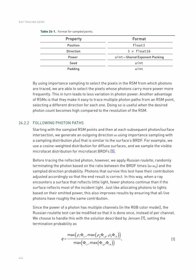
414
By using importance sampling to select the pixels in the RSM from which photons are traced, we are able to select the pixels whose photons carry more power more frequently. This in turn leads to less variation in photon power. Another advantage of RSMs is that they make it easy to trace multiple photon paths from an RSM point, selecting a different direction for each one. Doing so is useful when the desired photon count becomes high compared to the resolution of the RSM.
24.2.2 FOLLOWING PHOTON PATHS
Starting with the sampled RSM points and then at each subsequent photon/surface intersection, we generate an outgoing direction ω using importance sampling with a sampling distribution p(ω) that is similar to the surface’s BRDF. For example, we use a cosine-weighted distribution for diffuse surfaces, and we sample the visible microfacet distribution for microfacet BRDFs [5].
Before tracing the reflected photon, however, we apply Russian roulette, randomly terminating the photon based on the ratio between the BRDF times (ω⋅ωg) and the sampled direction probability. Photons that survive this test have their contribution adjusted accordingly so that the end result is correct. In this way, when a ray encounters a surface that reflects little light, fewer photons continue than if the surface reflects most of the incident light. Just like allocating photons to lights based on their emitted power, this also improves results by ensuring that all live photons have roughly the same contribution.
Since the power of a photon has multiple channels (in the RGB color model), the Russian roulette test can be modified so that it is done once, instead of per channel. We choose to handle this with the solution described by Jensen [7], setting the termination probability as
( )( )( )( )
r i r g i g b i b
i r i g i b
, ,q
, ,
, , ,
, , ,
max max,
max max
r r rF F F=
F F F (1)
Table 24-1. Format for sampled points.
RAY TRACING GEMS
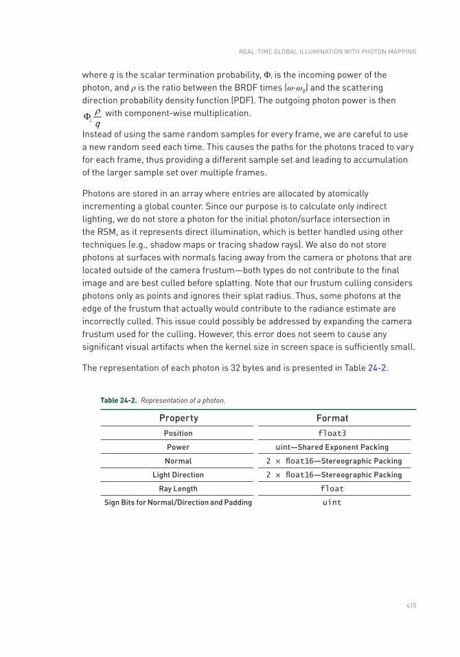
415
where q is the scalar termination probability, Φi is the incoming power of the photon, and ρ is the ratio between the BRDF times (ω⋅ωg) and the scattering direction probability density function (PDF). The outgoing photon power is then
i qr
F with component-wise multiplication.
Instead of using the same random samples for every frame, we are careful to use a new random seed each time. This causes the paths for the photons traced to vary for each frame, thus providing a different sample set and leading to accumulation of the larger sample set over multiple frames.
Photons are stored in an array where entries are allocated by atomically incrementing a global counter. Since our purpose is to calculate only indirect lighting, we do not store a photon for the initial photon/surface intersection in the RSM, as it represents direct illumination, which is better handled using other techniques (e.g., shadow maps or tracing shadow rays). We also do not store photons at surfaces with normals facing away from the camera or photons that are located outside of the camera frustum—both types do not contribute to the final image and are best culled before splatting. Note that our frustum culling considers photons only as points and ignores their splat radius. Thus, some photons at the edge of the frustum that actually would contribute to the radiance estimate are incorrectly culled. This issue could possibly be addressed by expanding the camera frustum used for the culling. However, this error does not seem to cause any significant visual artifacts when the kernel size in screen space is sufficiently small.
The representation of each photon is 32 bytes and is presented in Table 24-2.
Table 24-2. Representation of a photon.
REAL-TIME GLOBAL ILLUMINATION WITH PHOTON MAPPING
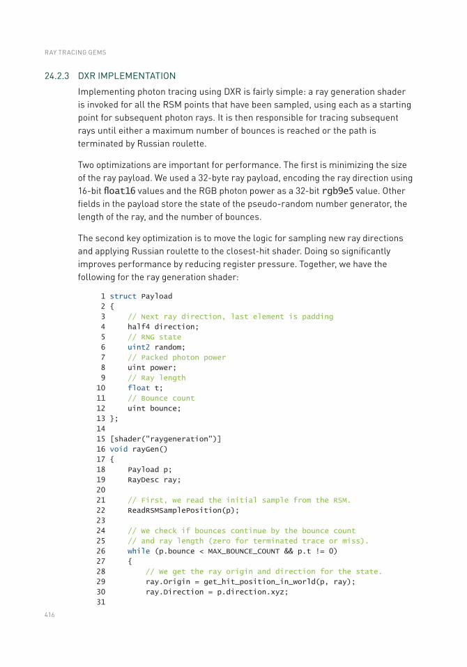
416
24.2.3 DXR IMPLEMENTATION
Implementing photon tracing using DXR is fairly simple: a ray generation shader is invoked for all the RSM points that have been sampled, using each as a starting point for subsequent photon rays. It is then responsible for tracing subsequent rays until either a maximum number of bounces is reached or the path is terminated by Russian roulette.
Two optimizations are important for performance. The first is minimizing the size of the ray payload. We used a 32-byte ray payload, encoding the ray direction using 16-bit float16 values and the RGB photon power as a 32-bit rgb9e5 value. Other fields in the payload store the state of the pseudo-random number generator, the length of the ray, and the number of bounces.
The second key optimization is to move the logic for sampling new ray directions and applying Russian roulette to the closest-hit shader. Doing so significantly improves performance by reducing register pressure. Together, we have the following for the ray generation shader:
1 struct Payload
2
3 // Next ray direction, last element is padding
4 half4 direction;
5 // RNG state
6 uint2 random;
7 // Packed photon power
8 uint power;
9 // Ray length
10 float t;
11 // Bounce count
12 uint bounce;
13 ;
14
15 [shader("raygeneration")]
16 void rayGen()
17
18 Payload p;
19 RayDesc ray;
20
21 // First, we read the initial sample from the RSM.
22 ReadRSMSamplePosition(p);
23
24 // We check if bounces continue by the bounce count
25 // and ray length (zero for terminated trace or miss).
26 while (p.bounce < MAX_BOUNCE_COUNT && p.t != 0)
27
28 // We get the ray origin and direction for the state.
29 ray.Origin = get_hit_position_in_world(p, ray);
30 ray.Direction = p.direction.xyz;
31
RAY TRACING GEMS
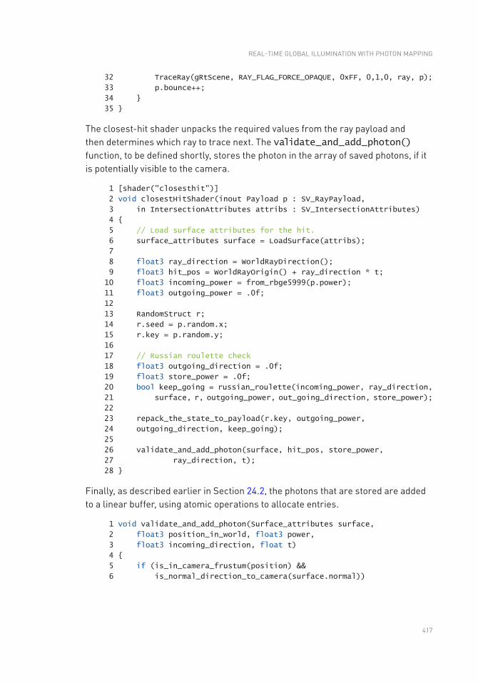
417
32 TraceRay(gRtScene, RAY_FLAG_FORCE_OPAQUE, 0xFF, 0,1,0, ray, p);
33 p.bounce++;
34
35
The closest-hit shader unpacks the required values from the ray payload and then determines which ray to trace next. The validate_and_add_photon() function, to be defined shortly, stores the photon in the array of saved photons, if it is potentially visible to the camera.
1 [shader("closesthit")]
2 void closestHitShader(inout Payload p : SV_RayPayload,
3 in IntersectionAttributes attribs : SV_IntersectionAttributes)
4
5 // Load surface attributes for the hit.
6 surface_attributes surface = LoadSurface(attribs);
7
8 float3 ray_direction = WorldRayDirection();
9 float3 hit_pos = WorldRayOrigin() + ray_direction * t;
10 float3 incoming_power = from_rbge5999(p.power);
11 float3 outgoing_power = .0f;
12
13 RandomStruct r;
14 r.seed = p.random.x;
15 r.key = p.random.y;
16
17 // Russian roulette check
18 float3 outgoing_direction = .0f;
19 float3 store_power = .0f;
20 bool keep_going = russian_roulette(incoming_power, ray_direction,
21 surface, r, outgoing_power, out_going_direction, store_power);
22
23 repack_the_state_to_payload(r.key, outgoing_power,
24 outgoing_direction, keep_going);
25
26 validate_and_add_photon(surface, hit_pos, store_power,
27 ray_direction, t);
28
Finally, as described earlier in Section 24.2, the photons that are stored are added to a linear buffer, using atomic operations to allocate entries.
1 void validate_and_add_photon(Surface_attributes surface,
2 float3 position_in_world, float3 power,
3 float3 incoming_direction, float t)
4
5 if (is_in_camera_frustum(position) &&
6 is_normal_direction_to_camera(surface.normal))
REAL-TIME GLOBAL ILLUMINATION WITH PHOTON MAPPING
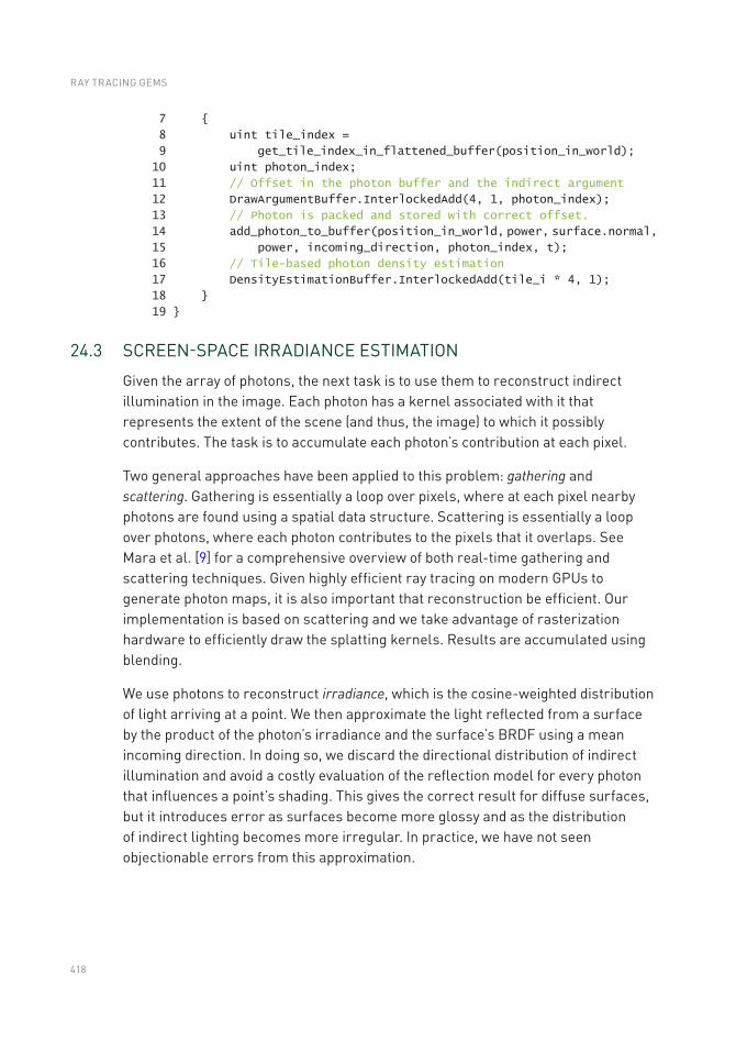
418
7
8 uint tile_index =
9 get_tile_index_in_flattened_buffer(position_in_world);
10 uint photon_index;
11 // Offset in the photon buffer and the indirect argument
12 DrawArgumentBuffer.InterlockedAdd(4, 1, photon_index);
13 // Photon is packed and stored with correct offset.
14 add_photon_to_buffer(position_in_world, power, surface.normal,
15 power, incoming_direction, photon_index, t);
16 // Tile-based photon density estimation
17 DensityEstimationBuffer.InterlockedAdd(tile_i * 4, 1);
18
19
24.3 SCREEN-SPACE IRRADIANCE ESTIMATION
Given the array of photons, the next task is to use them to reconstruct indirect illumination in the image. Each photon has a kernel associated with it that represents the extent of the scene (and thus, the image) to which it possibly contributes. The task is to accumulate each photon’s contribution at each pixel.
Two general approaches have been applied to this problem: gathering and scattering. Gathering is essentially a loop over pixels, where at each pixel nearby photons are found using a spatial data structure. Scattering is essentially a loop over photons, where each photon contributes to the pixels that it overlaps. See Mara et al. [9] for a comprehensive overview of both real-time gathering and scattering techniques. Given highly efficient ray tracing on modern GPUs to generate photon maps, it is also important that reconstruction be efficient. Our implementation is based on scattering and we take advantage of rasterization hardware to efficiently draw the splatting kernels. Results are accumulated using blending.
We use photons to reconstruct irradiance, which is the cosine-weighted distribution of light arriving at a point. We then approximate the light reflected from a surface by the product of the photon’s irradiance and the surface’s BRDF using a mean incoming direction. In doing so, we discard the directional distribution of indirect illumination and avoid a costly evaluation of the reflection model for every photon that influences a point’s shading. This gives the correct result for diffuse surfaces, but it introduces error as surfaces become more glossy and as the distribution of indirect lighting becomes more irregular. In practice, we have not seen objectionable errors from this approximation.
RAY TRACING GEMS
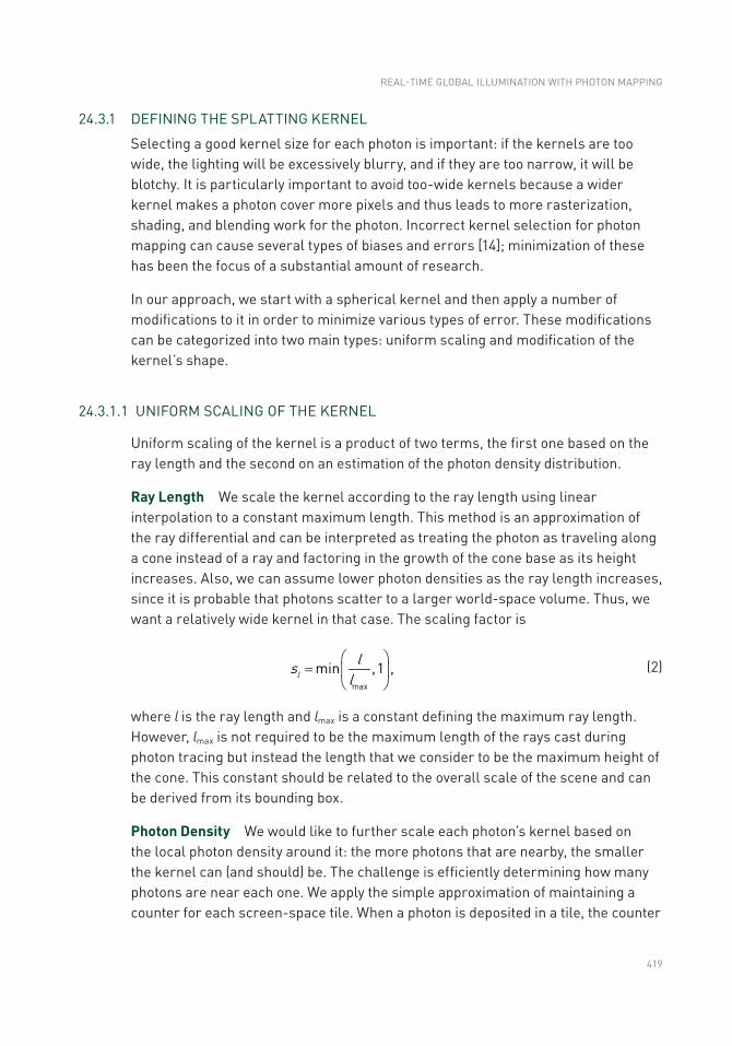
419
24.3.1 DEFINING THE SPLATTING KERNEL
Selecting a good kernel size for each photon is important: if the kernels are too wide, the lighting will be excessively blurry, and if they are too narrow, it will be blotchy. It is particularly important to avoid too-wide kernels because a wider kernel makes a photon cover more pixels and thus leads to more rasterization, shading, and blending work for the photon. Incorrect kernel selection for photon mapping can cause several types of biases and errors [14]; minimization of these has been the focus of a substantial amount of research.
In our approach, we start with a spherical kernel and then apply a number of modifications to it in order to minimize various types of error. These modifications can be categorized into two main types: uniform scaling and modification of the kernel’s shape.
24.3.1.1 UNIFORM SCALING OF THE KERNEL
Uniform scaling of the kernel is a product of two terms, the first one based on the ray length and the second on an estimation of the photon density distribution.
Ray Length We scale the kernel according to the ray length using linear interpolation to a constant maximum length. This method is an approximation of the ray differential and can be interpreted as treating the photon as traveling along a cone instead of a ray and factoring in the growth of the cone base as its height increases. Also, we can assume lower photon densities as the ray length increases, since it is probable that photons scatter to a larger world-space volume. Thus, we want a relatively wide kernel in that case. The scaling factor is
l
lslmax
min ,1 ,æ ö
= ç ÷è ø
(2)
where l is the ray length and lmax is a constant defining the maximum ray length. However, lmax is not required to be the maximum length of the rays cast during photon tracing but instead the length that we consider to be the maximum height of the cone. This constant should be related to the overall scale of the scene and can be derived from its bounding box.
Photon Density We would like to further scale each photon’s kernel based on the local photon density around it: the more photons that are nearby, the smaller the kernel can (and should) be. The challenge is efficiently determining how many photons are near each one. We apply the simple approximation of maintaining a counter for each screen-space tile. When a photon is deposited in a tile, the counter
REAL-TIME GLOBAL ILLUMINATION WITH PHOTON MAPPING
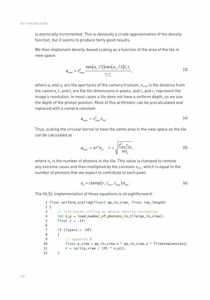
420
is atomically incremented. This is obviously a crude approximation of the density function, but it seems to produce fairly good results.
We then implement density-based scaling as a function of the area of the tile in view space:
( ) ( )x y x y
x y
t ta z
r r2
view view
tan / 2 tan / 2,
a a= (3)
where αx and αy are the apertures of the camera frustum, zview is the distance from the camera, tx and ty are the tile dimensions in pixels, and rx and ry represent the image’s resolution. In most cases a tile does not have a uniform depth, so we use the depth of the photon position. Most of this arithmetic can be precalculated and replaced with a camera constant:
a z c2view view tile.= (4)
Thus, scaling the circular kernel to have the same area in the view space as the tile can be calculated as
pp
z ca r n r
n
22 view tile
view , ,= p =p
(5)
where np is the number of photons in the tile. This value is clamped to remove any extreme cases and then multiplied by the constant ntile, which is equal to the number of photons that we expect to contribute to each pixel:
( )min max tileclamp .ds r , r , r n= (6)
The HLSL implementation of these equations is straightforward:
1 float uniform_scaling(float3 pp_in_view, float ray_length)
2
3 // Tile-based culling as photon density estimation
4 int n_p = load_number_of_photons_in_tile(pp_in_view);
5 float r = .1f;
6
7 if (layers > .0f)
8
9 // Equation 5
10 float a_view = pp_in_view.z * pp_in_view.z * TileAreaConstant;
11 r = sqrt(a_view / (PI * n_p));
12
RAY TRACING GEMS
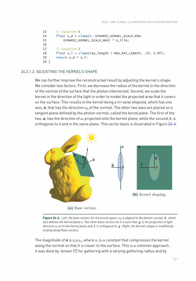
421
13 // Equation 6
14 float s_d = clamp(r, DYNAMIC_KERNEL_SCALE_MIN,
15 DYNAMIC_KERNEL_SCALE_MAX) * n_tile;
16
17 // Equation 2
18 float s_l = clamp(ray_length / MAX_RAY_LENGTH, .1f, 1.0f);
19 return s_d * s_l;
20
24.3.1.2 ADJUSTING THE KERNEL’S SHAPE
We can further improve the reconstructed result by adjusting the kernel’s shape. We consider two factors. First, we decrease the radius of the kernel in the direction of the normal of the surface that the photon intersected. Second, we scale the kernel in the direction of the light in order to model the projected area that it covers on the surface. This results in the kernel being a tri-axial ellipsoid, which has one axis, n, that has the direction ωg of the normal. The other two axes are placed on a tangent plane defined by the photon normal, called the kernel plane. The first of the two, u, has the direction of ωi projected onto the kernel plane, while the second, t, is orthogonal to it and in the same plane. This vector basis is illustrated in Figure 24-4.
The magnitude of n is snslsd, where sn is a constant that compresses the kernel along the normal so that it is closer to the surface. This is a common approach: it was done by Jensen [7] for gathering with a varying gathering radius and by
Figure 24-4. Left: the base vectors for the kernel space: ωg is aligned to the photon normal n , which also defines the kernel plane π. Two other basis vectors lie in π such that u is the projection of light direction ωi on to the kernel plane and t is orthogonal to u . Right: the kernel’s shape is modified by scaling along those vectors.
REAL-TIME GLOBAL ILLUMINATION WITH PHOTON MAPPING
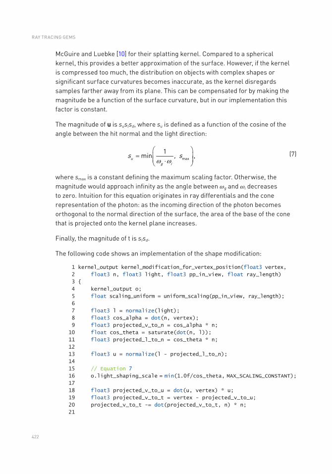
422
McGuire and Luebke [10] for their splatting kernel. Compared to a spherical kernel, this provides a better approximation of the surface. However, if the kernel is compressed too much, the distribution on objects with complex shapes or significant surface curvatures becomes inaccurate, as the kernel disregards samples farther away from its plane. This can be compensated for by making the magnitude be a function of the surface curvature, but in our implementation this factor is constant.
The magnitude of u is suslsd, where su is defined as a function of the cosine of the angle between the hit normal and the light direction:
u
g i
s , smax
1min ,w w
æ ö= ç ÷ç ÷×è ø
(7)
where smax is a constant defining the maximum scaling factor. Otherwise, the magnitude would approach infinity as the angle between ωg and ωi decreases to zero. Intuition for this equation originates in ray differentials and the cone representation of the photon: as the incoming direction of the photon becomes orthogonal to the normal direction of the surface, the area of the base of the cone that is projected onto the kernel plane increases.
Finally, the magnitude of t is slsd.
The following code shows an implementation of the shape modification:
1 kernel_output kernel_modification_for_vertex_position(float3 vertex,
2 float3 n, float3 light, float3 pp_in_view, float ray_length)
3
4 kernel_output o;
5 float scaling_uniform = uniform_scaling(pp_in_view, ray_length);
6
7 float3 l = normalize(light);
8 float3 cos_alpha = dot(n, vertex);
9 float3 projected_v_to_n = cos_alpha * n;
10 float cos_theta = saturate(dot(n, l));
11 float3 projected_l_to_n = cos_theta * n;
12
13 float3 u = normalize(l - projected_l_to_n);
14
15 // Equation 7
16 o.light_shaping_scale = min(1.0f/cos_theta, MAX_SCALING_CONSTANT);
17
18 float3 projected_v_to_u = dot(u, vertex) * u;
19 float3 projected_v_to_t = vertex - projected_v_to_u;
20 projected_v_to_t -= dot(projected_v_to_t, n) * n;
21
RAY TRACING GEMS
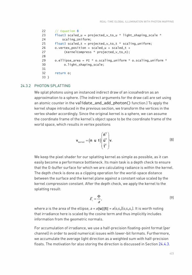
423
22 // Equation 8
23 float3 scaled_u = projected_v_to_u * light_shaping_scale *
24 scaling_Uniform;
25 float3 scaled_t = projected_v_to_t * scaling_uniform;
26 o.vertex_position = scaled_u + scaled_t +
27 (KernelCompress * projected_v_to_n);
28
29 o.ellipse_area = PI * o.scaling_uniform * o.scaling_uniform *
30 o.light_shaping_scale;
31
32 return o;
33
24.3.2 PHOTON SPLATTING
We splat photons using an instanced indirect draw of an icosahedron as an approximation to a sphere. (The indirect arguments for the draw call are set using an atomic counter in the validate_and_add_photon() function.) To apply the kernel shape introduced in the previous section, we transform the vertices in the vertex shader accordingly. Since the original kernel is a sphere, we can assume the coordinate frame of the kernel’s object space to be the coordinate frame of the world space, which results in vertex positions
( )kernel
ˆˆ .ˆ
æ öç ÷
= ç ÷ç ÷è ø
T
T
T
nv n u t u v
t
(8)
We keep the pixel shader for our splatting kernel as simple as possible, as it can easily become a performance bottleneck. Its main task is a depth check to ensure that the G-buffer surface for which we are calculating radiance is within the kernel. The depth check is done as a clipping operation for the world-space distance between the surface and the kernel plane against a constant value scaled by the kernel compression constant. After the depth check, we apply the kernel to the splatting result:
iE
a,F
= (9)
where a is the area of the ellipse, a = π‖u‖‖t‖ = π(slsd)(slsdsu). It is worth noting that irradiance here is scaled by the cosine term and thus implicitly includes information from the geometric normals.
For accumulation of irradiance, we use a half-precision floating-point format (per channel) in order to avoid numerical issues with lower-bit formats. Furthermore, we accumulate the average light direction as a weighted sum with half-precision floats. The motivation for also storing the direction is discussed in Section 24.4.3.
REAL-TIME GLOBAL ILLUMINATION WITH PHOTON MAPPING
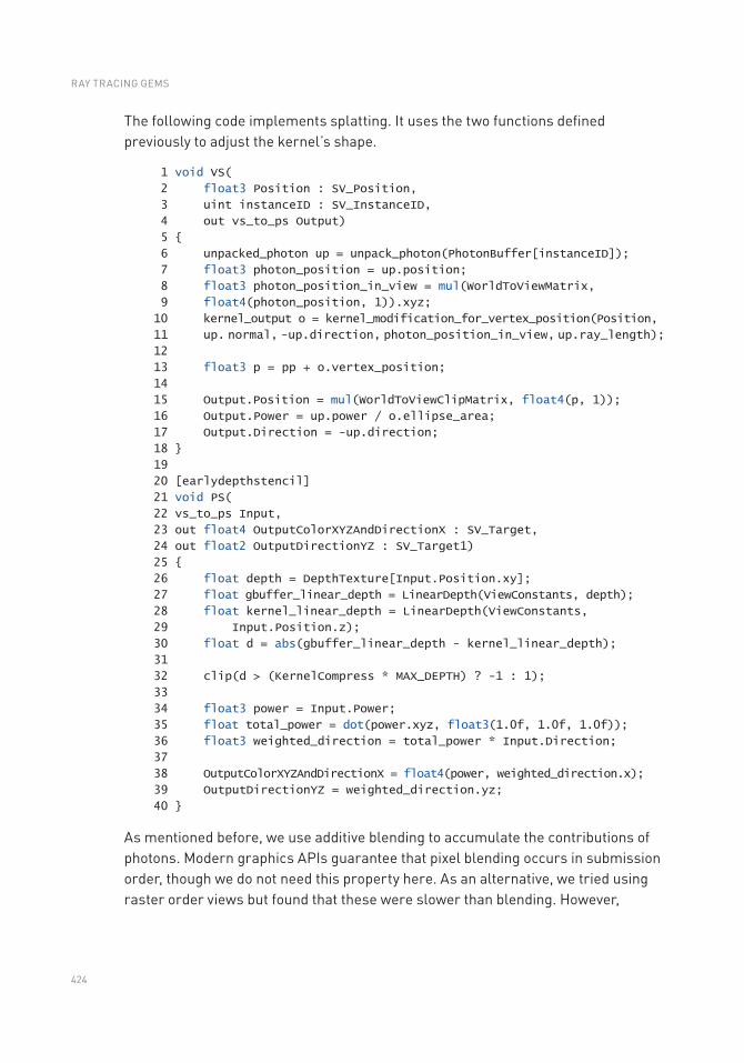
424
The following code implements splatting. It uses the two functions defined previously to adjust the kernel’s shape.
1 void VS(
2 float3 Position : SV_Position,
3 uint instanceID : SV_InstanceID,
4 out vs_to_ps Output)
5
6 unpacked_photon up = unpack_photon(PhotonBuffer[instanceID]);
7 float3 photon_position = up.position;
8 float3 photon_position_in_view = mul(WorldToViewMatrix,
9 float4(photon_position, 1)).xyz;
10 kernel_output o = kernel_modification_for_vertex_position(Position,
11 up. normal, -up.direction, photon_position_in_view, up.ray_length);
12
13 float3 p = pp + o.vertex_position;
14
15 Output.Position = mul(WorldToViewClipMatrix, float4(p, 1));
16 Output.Power = up.power / o.ellipse_area;
17 Output.Direction = -up.direction;
18
19
20 [earlydepthstencil]
21 void PS(
22 vs_to_ps Input,
23 out float4 OutputColorXYZAndDirectionX : SV_Target,
24 out float2 OutputDirectionYZ : SV_Target1)
25
26 float depth = DepthTexture[Input.Position.xy];
27 float gbuffer_linear_depth = LinearDepth(ViewConstants, depth);
28 float kernel_linear_depth = LinearDepth(ViewConstants,
29 Input.Position.z);
30 float d = abs(gbuffer_linear_depth - kernel_linear_depth);
31
32 clip(d > (KernelCompress * MAX_DEPTH) ? -1 : 1);
33
34 float3 power = Input.Power;
35 float total_power = dot(power.xyz, float3(1.0f, 1.0f, 1.0f));
36 float3 weighted_direction = total_power * Input.Direction;
37
38 OutputColorXYZAndDirectionX = float4(power, weighted_direction.x);
39 OutputDirectionYZ = weighted_direction.yz;
40
As mentioned before, we use additive blending to accumulate the contributions of photons. Modern graphics APIs guarantee that pixel blending occurs in submission order, though we do not need this property here. As an alternative, we tried using raster order views but found that these were slower than blending. However,
RAY TRACING GEMS
425
using floating- point atomic intrinsics, which are available on NVIDIA GPUs as an extension, did result in improved performance in situations when many photons overlap in screen space (a common scenario for caustics).
24.3.2.1 OPTIMIZING SPLATTING USING REDUCED RESOLUTION
Splatting can be an expensive process, which is especially the case when rendering high-resolution images. We found that reducing image resolution to half of the native rendering resolution did not cause a noticeable decrease in visual quality for the final result and gave a significant performance benefit. Using lower resolution does require a change to the depth clipping in the pixel shader to eliminate irradiance bleeding between surfaces: the half-resolution depth stencil used for stencil drawing should be downscaled using the closest pixel to the camera, but the depth used in pixel shader clipping should be downscaled using the farthest pixel from the camera. Hence, we draw the splatting kernel for only those pixels that are entirely within the full-resolution kernel. This causes jagged edges in the splatting result, but they are removed by the filtering.
24.4 FILTERING
As typical for real-time Monte Carlo rendering methods, it is necessary to apply image filtering algorithms to compensate for the low sample count. Although there have been significant advances in denoising in recent years, the noise caused by photon distribution kernels is quite different from the high-frequency noise that path tracing exhibits and that has been the main focus of denoising efforts. Thus, a different solution is required.
We use both temporal and spatial accumulation of samples with geometry-based edge-stopping functions. Our approach is based on previous work by Dammertz et al. [4] and Schied et al. [13], with our implementation using an edge-avoiding À-Trous wavelet transform for spatial filtering. Because indirect lighting is generally low frequency, we considered filtering at a lower resolution to decrease the computation cost, but we encountered artifacts due to G-buffer discrepancies and so reverted to filtering at the final resolution.
Both our temporal and spatial filtering algorithms use edge-stopping functions based on the difference in depth between two pixels and the difference in their surface normals. These functions, based on those of Schied et al. [13], attempt to prevent filtering across geometric boundaries by generating weights based on the
REAL-TIME GLOBAL ILLUMINATION WITH PHOTON MAPPING
426
surface attributes of two different pixels p and q. The depth difference weight wz is defined by
( ) ( ) ( )( )( )z
z
z P z Qw P,Q
P P Qexp ,
s e
æ ö-ç ÷= -ç ÷Ñ - +è øz
(10)
where z(P) is the screen-space depth at a pixel location P and ∇z(P) is the depth gradient vector. After experimentation σz = 1 was found to work well.
Next, the normal difference weight wn accounts for the difference of the surface normals:
( ) ( ) ( )( ) n
nw P,Q , P Qmax 0 ,ˆ ˆs
= ×n n (11)
where we found σn = 32 to work well.
24.4.1 TEMPORAL FILTERING
Temporal filtering improves image quality by accumulating values from previous frames. It is implemented by reprojecting the previous frame’s filtered irradiance values using velocity vectors and then at every pixel p computing an exponentially moving average between the previous frame’s reprojected filtered irradiance value
( )i PE 1- and the irradiance value Ei(P) computed using splatting, giving a temporally
filtered irradiance ( )i PE :
( ) ( ) ( ) ( )11 .i i iP E P E PE a a -= - + (12)
This is Karis’s temporal antialiasing (TAA) approach [8] applied to irradiance.
Using a constant value for α would cause severe ghosting artifacts, as the temporal filtering would not account for disocclusions, moving geometry, or moving lights. However, because the irradiance values Ei at a pixel can vary significantly between frames, color-space clipping methods used in TAA are not well suited for them. Therefore, we rely on geometry-based methods and define α using the edge-stopping functions as
( ) ( )z nw P,Q w P,Q0.95 ,a = (13)
where P is a current pixel sample and Q is the projected sample from the previous frame. To evaluate the weight functions, it is necessary to maintain the normal and depth data from the G-buffer of the previous frame. If the resolution of the splatting target is lower than the filtering target, we upscale the splatting result at the beginning of the temporal filtering pass with bilinear sampling.
RAY TRACING GEMS
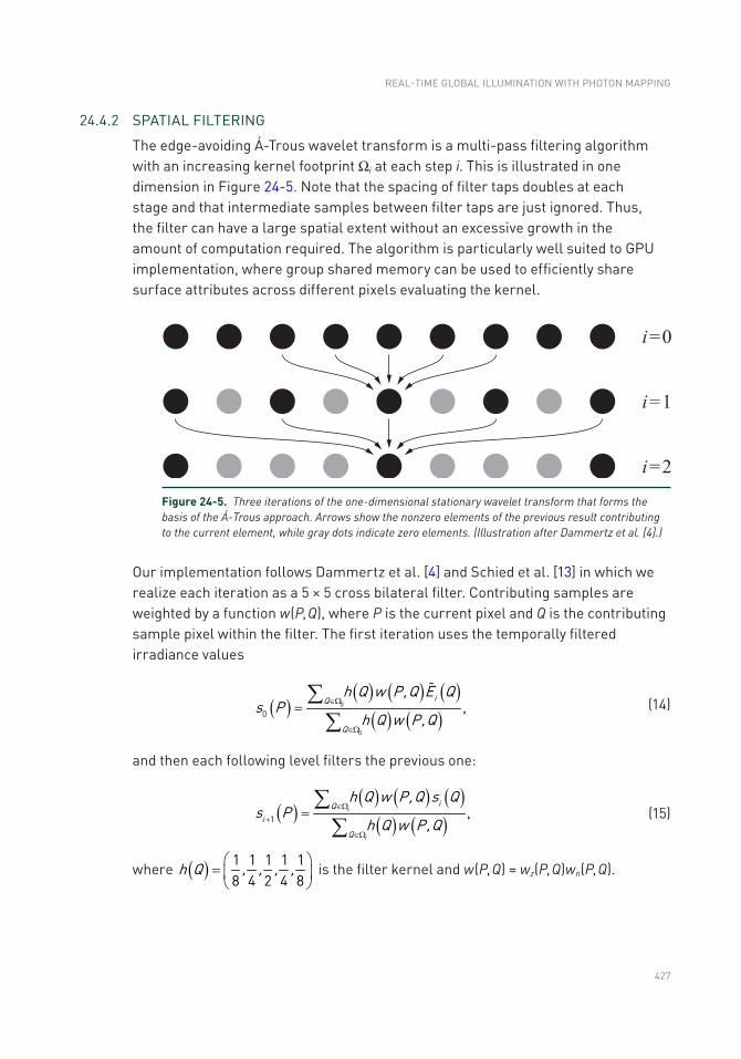
427
24.4.2 SPATIAL FILTERING
The edge-avoiding Á-Trous wavelet transform is a multi-pass filtering algorithm with an increasing kernel footprint Ωi at each step i. This is illustrated in one dimension in Figure 24-5. Note that the spacing of filter taps doubles at each stage and that intermediate samples between filter taps are just ignored. Thus, the filter can have a large spatial extent without an excessive growth in the amount of computation required. The algorithm is particularly well suited to GPU implementation, where group shared memory can be used to efficiently share surface attributes across different pixels evaluating the kernel.
Our implementation follows Dammertz et al. [4] and Schied et al. [13] in which we realize each iteration as a 5 × 5 cross bilateral filter. Contributing samples are weighted by a function w(P, Q), where P is the current pixel and Q is the contributing sample pixel within the filter. The first iteration uses the temporally filtered irradiance values
( )( ) ( ) ( )
( ) ( )iQ
Q
h Q w P,Q E Qs P
h Q w P,Q0
0
0 ,ÎW
ÎW
=åå
(14)
and then each following level filters the previous one:
( )( ) ( ) ( )
( ) ( )i
i
iQi
Q
h Q w P,Q s Qs P
h Q w P,Q1 ,ÎW
+
ÎW
=åå
(15)
where ( )h Q , , , ,1 1 1 1 18 4 2 4 8
æ ö= ç ÷è ø
is the filter kernel and w(P, Q) = wz(P, Q)wn(P, Q).
Figure 24-5. Three iterations of the one-dimensional stationary wavelet transform that forms the basis of the Á-Trous approach. Arrows show the nonzero elements of the previous result contributing to the current element, while gray dots indicate zero elements. (Illustration after Dammertz et al. [4].)
REAL-TIME GLOBAL ILLUMINATION WITH PHOTON MAPPING
428
24.4.2.1 VARIANCE CLIPPING OF DETAIL COEFFICIENTS
To avoid blurring excessively, it is important to adapt the image filtering based on the accuracy of the image contents. For example, Schied et al. [13] use an estimate of variance as a part of their weight function. That works well for high-frequency noise but is unsuitable for the low-frequency noise from photon mapping. Therefore, we have developed a new filtering algorithm based on variance clipping of the differences between each stage of the Á-Trous transform.
The stationary wavelet transform (SWT) was originally introduced to combat one of the shortcomings of the discrete wavelet transform, that the transformation is not shift-invariant. This problem was solved by saving detail coefficients per pixel for each iteration. The detail coefficients can be defined by
i i id s s1 .+= - (16)
This makes the SWT inherently redundant. If we consider how to reconstruct the original signal, we have
n
n ii
s s d1
00
,-
=
= -å (17)
where n is the number of iterations. As we can see, to reconstruct the original signal we need only the sum of the detail coefficients. Doing so allows us to reduce the amount of required memory to two textures, each with the resolution of the original image. Nevertheless, this just leaves us at the same point where we started—the original unfiltered image.
However, we can apply variance clipping [12] to each of the detail coefficients before we add them in to the sum. This approach works well here, unlike with the unfiltered frame irradiance values Ei, because we are starting with temporally filtered values. We compute color-space boundaries (denoted by bi) based on the variance of irradiance within the spatial kernel. In turn, these boundaries are used for clipping the detail coefficients, and we compute a final filtered irradiance value as
( )n
n i i ii
E s d , b , b1
final0
clamp .-
=
= - -å (18)
Finally, we apply the filtered irradiance to the surfaces. As described earlier, we ignore the directional distribution of indirect lighting. Instead, we use the mean direction as the incoming light parameter to evaluate the BRDF. The irradiance is multiplied by the BRDF value retrieved:
L E ffinal final BRDF.= (19)
RAY TRACING GEMS
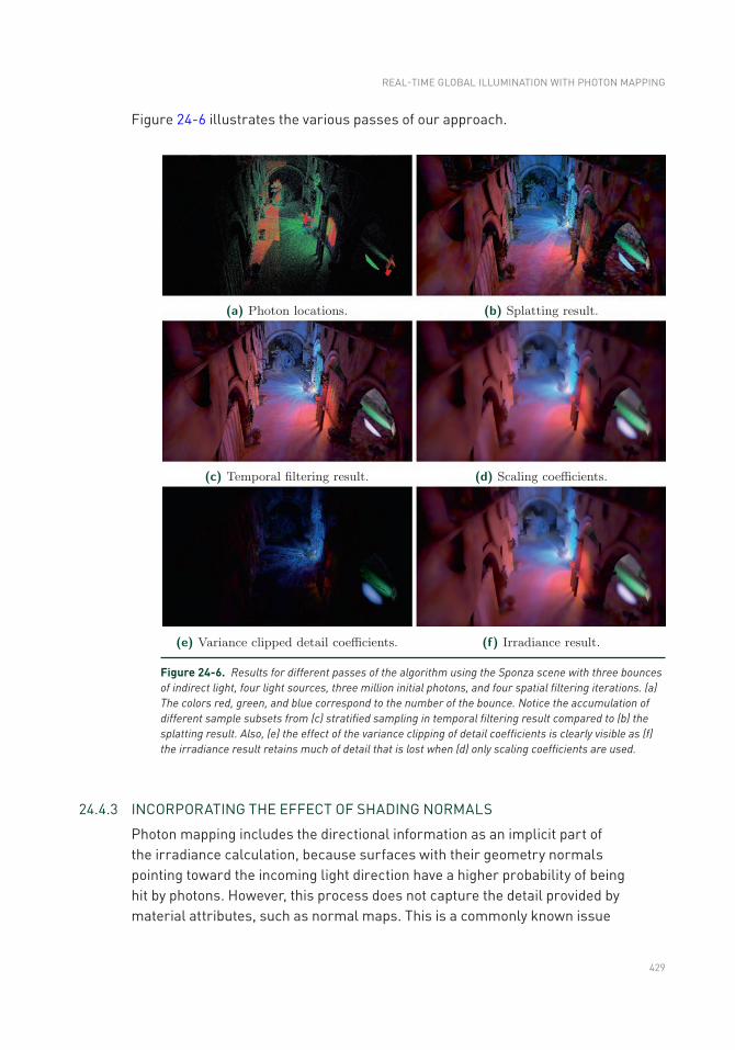
429
Figure 24-6 illustrates the various passes of our approach.
24.4.3 INCORPORATING THE EFFECT OF SHADING NORMALS
Photon mapping includes the directional information as an implicit part of the irradiance calculation, because surfaces with their geometry normals pointing toward the incoming light direction have a higher probability of being hit by photons. However, this process does not capture the detail provided by material attributes, such as normal maps. This is a commonly known issue
Figure 24-6. Results for different passes of the algorithm using the Sponza scene with three bounces of indirect light, four light sources, three million initial photons, and four spatial filtering iterations. (a) The colors red, green, and blue correspond to the number of the bounce. Notice the accumulation of different sample subsets from (c) stratified sampling in temporal filtering result compared to (b) the splatting result. Also, (e) the effect of the variance clipping of detail coefficients is clearly visible as (f) the irradiance result retains much of detail that is lost when (d) only scaling coefficients are used.
REAL-TIME GLOBAL ILLUMINATION WITH PHOTON MAPPING
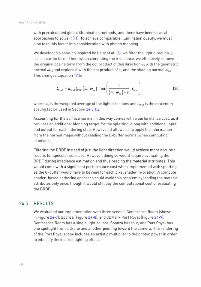
430
with precalculated global illumination methods, and there have been several approaches to solve it [11]. To achieve comparable illumination quality, we must also take this factor into consideration with photon mapping.
We developed a solution inspired by Heitz et al. [6]: we filter the light direction ωi as a separate term. Then, when computing the irradiance, we effectively remove the original cosine term from the dot product of this direction ωi with the geometric normal ωng and replace it with the dot product of ωi and the shading normal ωns. This changes Equation 19 to
( ) ( )i nsi ng
L E f , sfinal final BRDF max
1min ,w ww w e
æ öç ÷= ×ç ÷× +è ø
(20)
where ωi is the weighted average of the light directions and smax is the maximum scaling factor used in Section 24.3.1.2.
Accounting for the surface normal in this way comes with a performance cost, as it requires an additional blending target for the splatting, along with additional input and output for each filtering step. However, it allows us to apply the information from the normal maps without reading the G-buffer normal when computing irradiance.
Filtering the BRDF instead of just the light direction would achieve more accurate results for specular surfaces. However, doing so would require evaluating the BRDF during irradiance estimation and thus reading the material attributes. This would come with a significant performance cost when implemented with splatting, as the G-buffer would have to be read for each pixel shader invocation. A compute shader–based gathering approach could avoid this problem by loading the material attributes only once, though it would still pay the computational cost of evaluating the BRDF.
24.5 RESULTS
We evaluated our implementation with three scenes: Conference Room (shown in Figure 24-7), Sponza (Figure 24-8), and 3DMark Port Royal (Figure 24-9). Conference Room has a single light source, Sponza has four, and Port Royal has one spotlight from a drone and another pointing toward the camera. The rendering of the Port Royal scene includes an artistic multiplier to the photon power in order to intensify the indirect lighting effect.
RAY TRACING GEMS
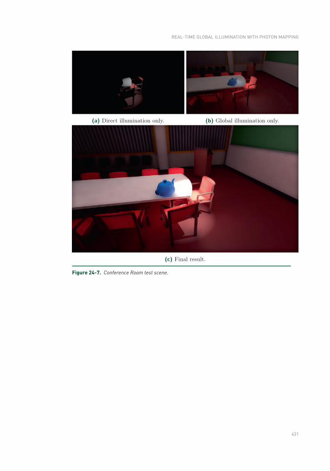
431
Figure 24-7. Conference Room test scene.
REAL-TIME GLOBAL ILLUMINATION WITH PHOTON MAPPING
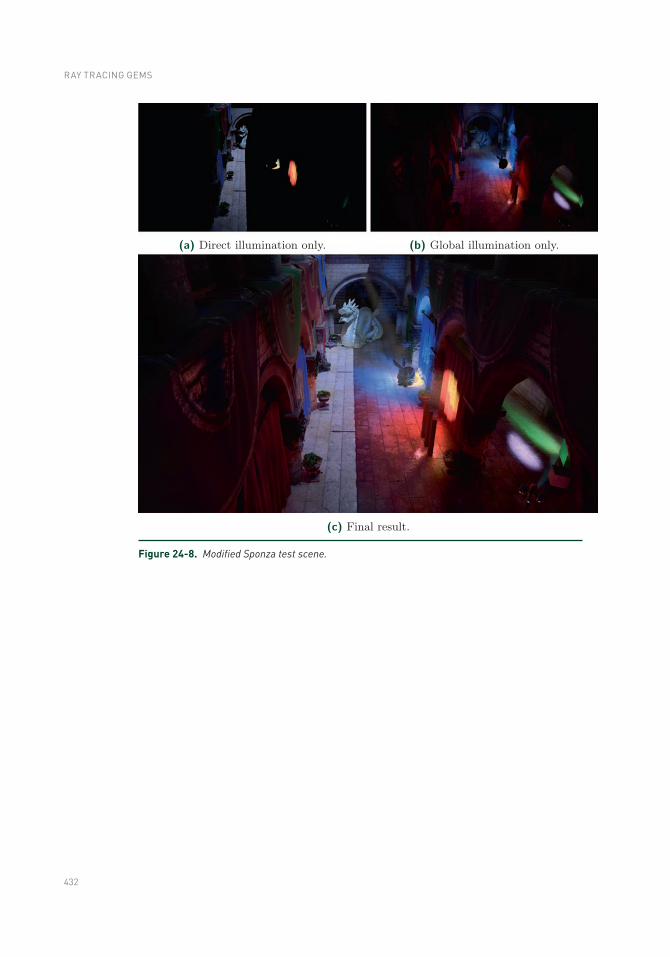
432
Figure 24-8. Modified Sponza test scene.
RAY TRACING GEMS
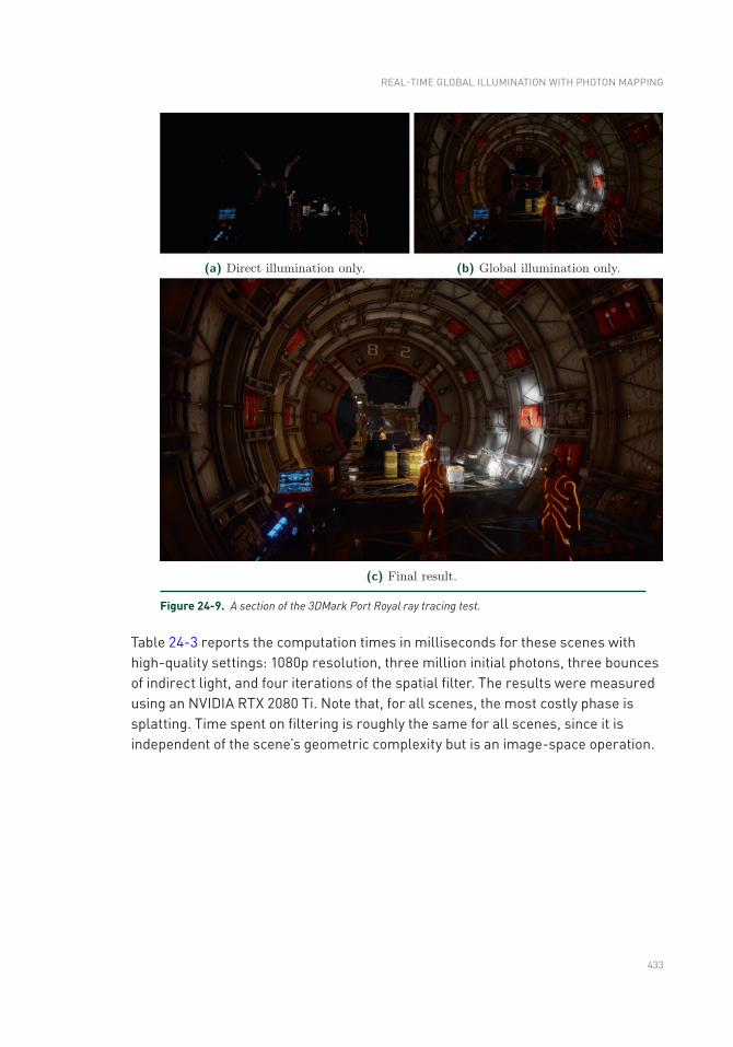
433
Table 24-3 reports the computation times in milliseconds for these scenes with high-quality settings: 1080p resolution, three million initial photons, three bounces of indirect light, and four iterations of the spatial filter. The results were measured using an NVIDIA RTX 2080 Ti. Note that, for all scenes, the most costly phase is splatting. Time spent on filtering is roughly the same for all scenes, since it is independent of the scene’s geometric complexity but is an image-space operation.
Figure 24-9. A section of the 3DMark Port Royal ray tracing test.
REAL-TIME GLOBAL ILLUMINATION WITH PHOTON MAPPING
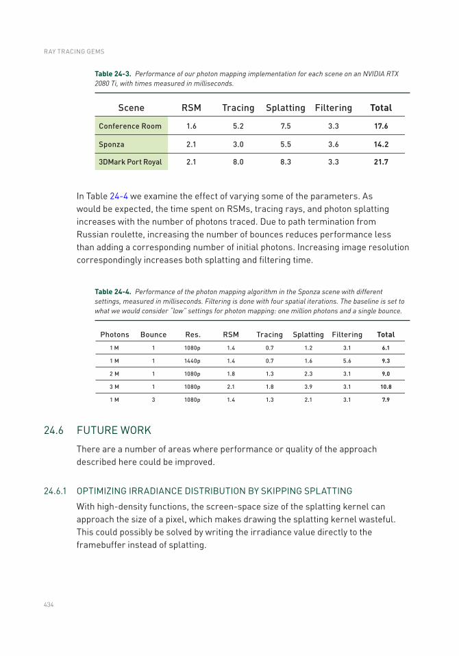
434
In Table 24-4 we examine the effect of varying some of the parameters. As would be expected, the time spent on RSMs, tracing rays, and photon splatting increases with the number of photons traced. Due to path termination from Russian roulette, increasing the number of bounces reduces performance less than adding a corresponding number of initial photons. Increasing image resolution correspondingly increases both splatting and filtering time.
24.6 FUTURE WORK
There are a number of areas where performance or quality of the approach described here could be improved.
24.6.1 OPTIMIZING IRRADIANCE DISTRIBUTION BY SKIPPING SPLATTING
With high-density functions, the screen-space size of the splatting kernel can approach the size of a pixel, which makes drawing the splatting kernel wasteful. This could possibly be solved by writing the irradiance value directly to the framebuffer instead of splatting.
Table 24-3. Performance of our photon mapping implementation for each scene on an NVIDIA RTX 2080 Ti, with times measured in milliseconds.
Table 24-4. Performance of the photon mapping algorithm in the Sponza scene with different settings, measured in milliseconds. Filtering is done with four spatial iterations. The baseline is set to what we would consider “low” settings for photon mapping: one million photons and a single bounce.
RAY TRACING GEMS
435
24.6.2 ADAPTIVE CONSTANTS FOR VARIANCE CLIPPING OF THE DETAIL COEFFICIENTS
Unfortunately, we cannot determine if the variance in the irradiance is caused by the low sample count or an actual difference in lighting conditions. This is partly mitigated by the larger sample set provided by stratified sampling. As these samples are accumulated using temporal filtering, the noise becomes visible in cases where temporal samples are being rejected. Therefore, it would be preferable to use less constricting variance clipping boundaries for these areas. Such a system could be implemented by scaling the variance clipping constant based on the weights that we use to define the accumulation of the temporal samples.
REFERENCES
[1] Clarberg, P., Jarosz, W., Akenine-Möller, T., and Jensen, H. W. Wavelet Importance Sampling: Efficiently Evaluating Products of Complex Functions. ACM Transactions on Graphics 24, 3 (2005), 1166–1175.
[2] Dachsbacher, C., and Stamminger, M. Reflective Shadow Maps. In Proceedings of the 2005 Symposium on Interactive 3D Graphics and Games (2005), pp. 203–231.
[3] Dachsbacher, C., and Stamminger, M. Splatting Indirect Illumination. In Proceedings of the 2006 Symposium on Interactive 3D Graphics and Games (2006), ACM, pp. 93–100.
[4] Dammertz, H., Sewtz, D., Hanika, J., and Lensch, H. Edge-Avoiding À-Trous Wavelet Transform for Fast Global Illumination Filtering. In Proceedings of High- Performance Graphics (2010), pp. 67–75.
[5] Heitz, E., and d’Eon, E. Importance Sampling Microfacet-Based BSDFs using the Distribution of Visible Normals. Computer Graphics Forum 33, 4 (2014), 103–112.
[6] Heitz, E., Hill, S., and McGuire, M. Combining Analytic Direct Illumination and Stochastic Shadows. In Proceedings of the ACM SIGGRAPH Symposium on Interactive 3D Graphics and Games (2018), pp. 2:1–2:11.
[7] Jensen, H. W. Realistic Image Synthesis Using Photon Mapping. A K Peters, 2001.
[8] Karis, B. High-Quality Temporal Supersampling. Advances in Real-Time Rendering in Games, SIGGRAPH Courses, 2014.
[9] Mara, M., Luebke, D., and McGuire, M. Toward Practical Real-Time Photon Mapping: Efficient GPU Density Estimation. In Proceedings of the ACM SIGGRAPH Symposium on Interactive 3D Graphics and Games (2013), pp. 71–78.
[10] McGuire, M., and Luebke, D. Hardware-Accelerated Global Illumination by Image Space Photon Mapping. In Proceedings of High-Performance Graphics (2009), pp. 77–89.
[11] O’Donnell, Y. Precomputed Global Illumination in Frostbite. Game Developers Conference, 2018.
REAL-TIME GLOBAL ILLUMINATION WITH PHOTON MAPPING

436
[12] Salvi, M. An Excursion in Temporal Supersampling. From the Lab Bench: Real-Time Rendering Advances from NVIDIA Research, Game Developers Conference, 2016.
[13] Schied, C., Kaplanyan, A., Wyman, C., Patney, A., Chaitanya, C. R. A., Burgess, J., Liu, S., Dachsbacher, C., Lefohn, A., and Salvi, M. Spatiotemporal Variance- Guided Filtering: Real-Time Reconstruction for Path-Traced Global Illumination. In Proceedings of High-Performance Graphics (2017), pp. 2:1–2:12.
[14] Schregle, R. Bias Compensation for Photon Maps. Computer Graphics Forum 22, 4 (2003), 729–742.
Open Access This chapter is licensed under the terms of the Creative Commons Attribution-NonCommercial-NoDerivatives 4.0 International License (http://creativecommons.org/licenses/by-nc-nd/4.0/), which permits any noncommercial use, sharing, distribution and
reproduction in any medium or format, as long as you give appropriate credit to the original author(s) and the source, provide a link to the Creative Commons license and indicate if you modified the licensed material. You do not have permission under this license to share adapted material derived from this chapter or parts of it.
The images or other third party material in this chapter are included in the chapter's Creative Commons license, unless indicated otherwise in a credit line to the material. If material is not included in the chapter's Creative Commons license and your intended use is not permitted by statutory regulation or exceeds the permitted use, you will need to obtain permission directly from the copyright holder.
RAY TRACING GEMS
437© NVIDIA 2019 E. Haines, T. Akenine-Möller (eds.), Ray Tracing Gems, https://doi.org/10.1007/978-1-4842-4427-2_25
CHAPTER 25
Hybrid Rendering for Real- Time Ray TracingColin Barré-Brisebois, Henrik Halén, Graham Wihlidal, Andrew Lauritzen, Jasper Bekkers, Tomasz Stachowiak, and Johan Andersson
SEED / Electronic Arts
ABSTRACT
This chapter describes the rendering pipeline developed for PICA PICA, a real-time ray tracing experiment featuring self-learning agents in a procedurally assembled world. PICA PICA showcases a hybrid rendering pipeline in which rasterization, compute, and ray tracing shaders work together to enable real-time visuals approaching the quality of offline path tracing.
The design behind the various stages of such a pipeline is described, including implementation details essential to the realization of PICA PICA’s hybrid ray tracing techniques. Advice on implementing the various ray tracing stages is provided, supplemented by pseudocode for ray traced shadows and ambient occlusion. A replacement to exponential averaging in the form of a reactive multi-scale mean estimator is also included. Even though PICA PICA’s world is lightly textured and small, this chapter describes the necessary building blocks of a hybrid rendering pipeline that could then be specialized for any AAA game. Ultimately, this chapter provides the reader with an overall good design to augment existing physically based deferred rendering pipelines with ray tracing, in a modular fashion that is compatible across visual styles.
25.1 HYBRID RENDERING PIPELINE OVERVIEW
PICA PICA [2, 3] features a hybrid rendering pipeline that relies on the rasterization and compute stages of the modern graphics pipeline, as well as the recently added ray tracing stage [23]. See Figure 25-1. The reader can see such results via a video available online [10]. Visualized as blocks in Figure 25-2, several aspects of such a pipeline are realized by a mix-and-match of the available graphical stages, and the pipeline takes advantage of each stage’s unique capabilities in a hybrid fashion.
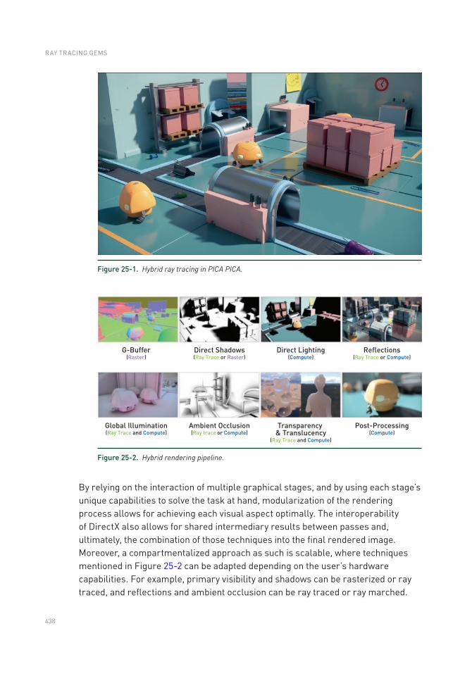
438
By relying on the interaction of multiple graphical stages, and by using each stage’s unique capabilities to solve the task at hand, modularization of the rendering process allows for achieving each visual aspect optimally. The interoperability of DirectX also allows for shared intermediary results between passes and, ultimately, the combination of those techniques into the final rendered image. Moreover, a compartmentalized approach as such is scalable, where techniques mentioned in Figure 25-2 can be adapted depending on the user’s hardware capabilities. For example, primary visibility and shadows can be rasterized or ray traced, and reflections and ambient occlusion can be ray traced or ray marched.
Figure 25-1. Hybrid ray tracing in PICA PICA.
Figure 25-2. Hybrid rendering pipeline.
RAY TRACING GEMS
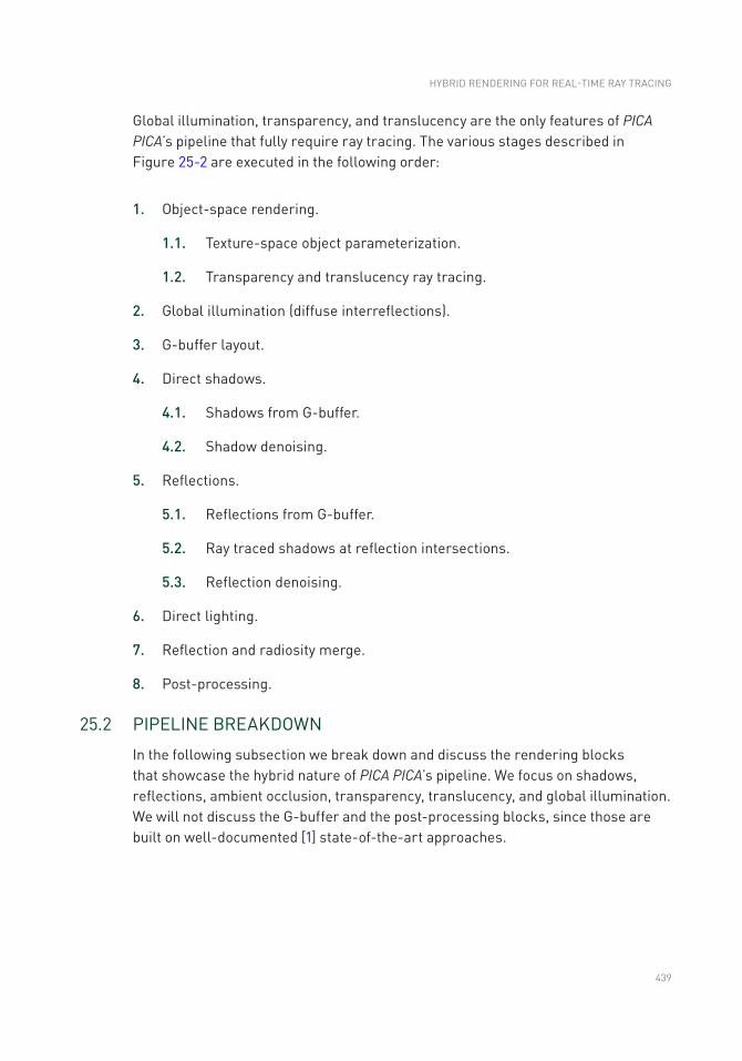
439
Global illumination, transparency, and translucency are the only features of PICA PICA’s pipeline that fully require ray tracing. The various stages described in Figure 25-2 are executed in the following order:
1. Object-space rendering.
1.1. Texture-space object parameterization.
1.2. Transparency and translucency ray tracing.
2. Global illumination (diffuse interreflections).
3. G-buffer layout.
4. Direct shadows.
4.1. Shadows from G-buffer.
4.2. Shadow denoising.
5. Reflections.
5.1. Reflections from G-buffer.
5.2. Ray traced shadows at reflection intersections.
5.3. Reflection denoising.
6. Direct lighting.
7. Reflection and radiosity merge.
8. Post-processing.
25.2 PIPELINE BREAKDOWN
In the following subsection we break down and discuss the rendering blocks that showcase the hybrid nature of PICA PICA’s pipeline. We focus on shadows, reflections, ambient occlusion, transparency, translucency, and global illumination. We will not discuss the G-buffer and the post-processing blocks, since those are built on well- documented [1] state-of-the-art approaches.
HYBRID RENDERING FOR REAL- TIME RAY TRACING
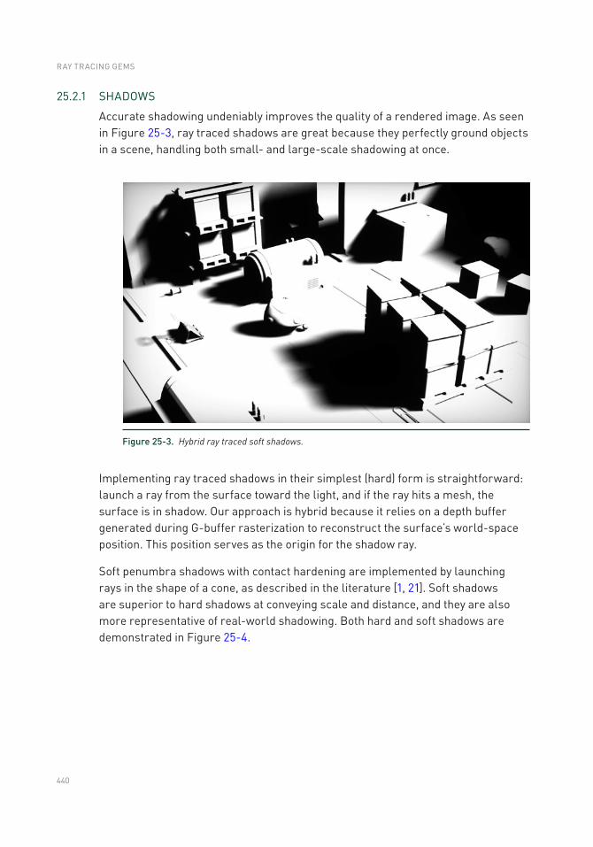
440
25.2.1 SHADOWS
Accurate shadowing undeniably improves the quality of a rendered image. As seen in Figure 25-3, ray traced shadows are great because they perfectly ground objects in a scene, handling both small- and large-scale shadowing at once.
Implementing ray traced shadows in their simplest (hard) form is straightforward: launch a ray from the surface toward the light, and if the ray hits a mesh, the surface is in shadow. Our approach is hybrid because it relies on a depth buffer generated during G-buffer rasterization to reconstruct the surface’s world-space position. This position serves as the origin for the shadow ray.
Soft penumbra shadows with contact hardening are implemented by launching rays in the shape of a cone, as described in the literature [1, 21]. Soft shadows are superior to hard shadows at conveying scale and distance, and they are also more representative of real-world shadowing. Both hard and soft shadows are demonstrated in Figure 25-4.
Figure 25-3. Hybrid ray traced soft shadows.
RAY TRACING GEMS
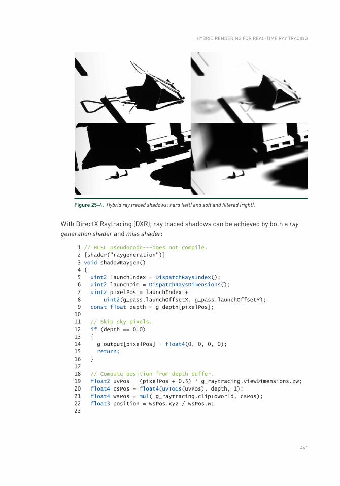
441
With DirectX Raytracing (DXR), ray traced shadows can be achieved by both a ray generation shader and miss shader:
1 // HLSL pseudocode---does not compile.
2 [shader("raygeneration")]
3 void shadowRaygen()
4
5 uint2 launchIndex = DispatchRaysIndex();
6 uint2 launchDim = DispatchRaysDimensions();
7 uint2 pixelPos = launchIndex +
8 uint2(g_pass.launchOffsetX, g_pass.launchOffsetY);
9 const float depth = g_depth[pixelPos];
10
11 // Skip sky pixels.
12 if (depth == 0.0)
13
14 g_output[pixelPos] = float4(0, 0, 0, 0);
15 return;
16
17
18 // Compute position from depth buffer.
19 float2 uvPos = (pixelPos + 0.5) * g_raytracing.viewDimensions.zw;
20 float4 csPos = float4(uvToCs(uvPos), depth, 1);
21 float4 wsPos = mul( g_raytracing.clipToWorld, csPos);
22 float3 position = wsPos.xyz / wsPos.w;
23
Figure 25-4. Hybrid ray traced shadows: hard (left) and soft and filtered (right).
HYBRID RENDERING FOR REAL- TIME RAY TRACING
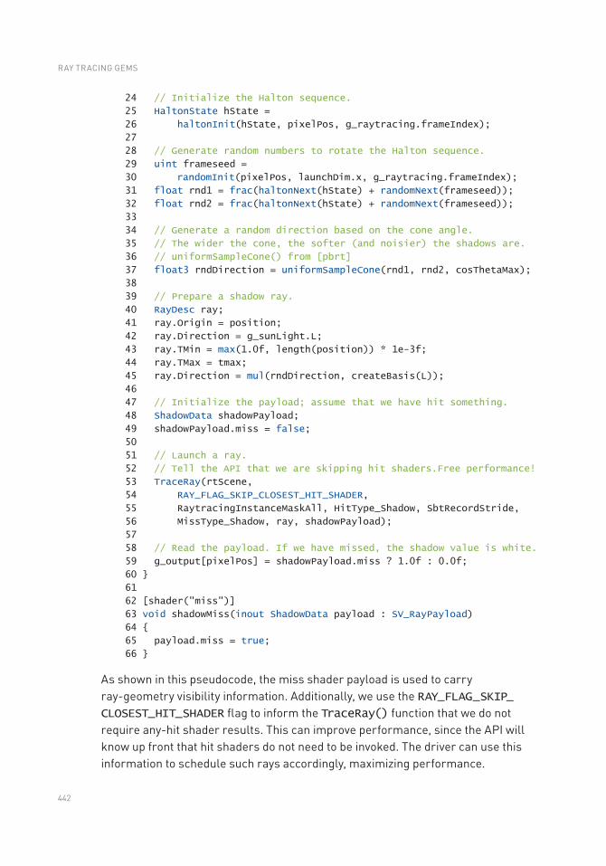
442
24 // Initialize the Halton sequence.
25 HaltonState hState =
26 haltonInit(hState, pixelPos, g_raytracing.frameIndex);
27
28 // Generate random numbers to rotate the Halton sequence.
29 uint frameseed =
30 randomInit(pixelPos, launchDim.x, g_raytracing.frameIndex);
31 float rnd1 = frac(haltonNext(hState) + randomNext(frameseed));
32 float rnd2 = frac(haltonNext(hState) + randomNext(frameseed));
33
34 // Generate a random direction based on the cone angle.
35 // The wider the cone, the softer (and noisier) the shadows are.
36 // uniformSampleCone() from [pbrt]
37 float3 rndDirection = uniformSampleCone(rnd1, rnd2, cosThetaMax);
38
39 // Prepare a shadow ray.
40 RayDesc ray;
41 ray.Origin = position;
42 ray.Direction = g_sunLight.L;
43 ray.TMin = max(1.0f, length(position)) * 1e-3f;
44 ray.TMax = tmax;
45 ray.Direction = mul(rndDirection, createBasis(L));
46
47 // Initialize the payload; assume that we have hit something.
48 ShadowData shadowPayload;
49 shadowPayload.miss = false;
50
51 // Launch a ray.
52 // Tell the API that we are skipping hit shaders.Free performance!
53 TraceRay(rtScene,
54 RAY_FLAG_SKIP_CLOSEST_HIT_SHADER,
55 RaytracingInstanceMaskAll, HitType_Shadow, SbtRecordStride,
56 MissType_Shadow, ray, shadowPayload);
57
58 // Read the payload. If we have missed, the shadow value is white.
59 g_output[pixelPos] = shadowPayload.miss ? 1.0f : 0.0f;
60
61
62 [shader("miss")]
63 void shadowMiss(inout ShadowData payload : SV_RayPayload)
64
65 payload.miss = true;
66
As shown in this pseudocode, the miss shader payload is used to carry ray-geometry visibility information. Additionally, we use the RAY_FLAG_SKIP_CLOSEST_HIT_SHADER flag to inform the TraceRay() function that we do not require any-hit shader results. This can improve performance, since the API will know up front that hit shaders do not need to be invoked. The driver can use this information to schedule such rays accordingly, maximizing performance.
RAY TRACING GEMS
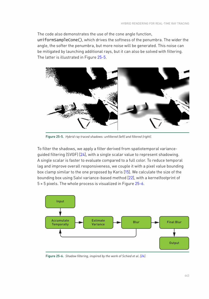
443
The code also demonstrates the use of the cone angle function, uniformSampleCone(), which drives the softness of the penumbra. The wider the angle, the softer the penumbra, but more noise will be generated. This noise can be mitigated by launching additional rays, but it can also be solved with filtering. The latter is illustrated in Figure 25-5.
Figure 25-5. Hybrid ray traced shadows: unfiltered (left) and filtered (right).
To filter the shadows, we apply a filter derived from spatiotemporal variance-guided filtering (SVGF) [24], with a single scalar value to represent shadowing. A single scalar is faster to evaluate compared to a full color. To reduce temporal lag and improve overall responsiveness, we couple it with a pixel value bounding box clamp similar to the one proposed by Karis [15]. We calculate the size of the bounding box using Salvi variance- based method [22], with a kernelfootprint of 5 × 5 pixels. The whole process is visualized in Figure 25-6.
Figure 25-6. Shadow filtering, inspired by the work of Schied et al. [24].
HYBRID RENDERING FOR REAL- TIME RAY TRACING
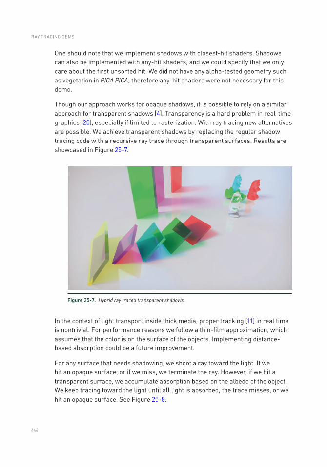
444
In the context of light transport inside thick media, proper tracking [11] in real time is nontrivial. For performance reasons we follow a thin-film approximation, which assumes that the color is on the surface of the objects. Implementing distance-based absorption could be a future improvement.
For any surface that needs shadowing, we shoot a ray toward the light. If we hit an opaque surface, or if we miss, we terminate the ray. However, if we hit a transparent surface, we accumulate absorption based on the albedo of the object. We keep tracing toward the light until all light is absorbed, the trace misses, or we hit an opaque surface. See Figure 25-8.
One should note that we implement shadows with closest-hit shaders. Shadows can also be implemented with any-hit shaders, and we could specify that we only care about the first unsorted hit. We did not have any alpha-tested geometry such as vegetation in PICA PICA, therefore any-hit shaders were not necessary for this demo.
Though our approach works for opaque shadows, it is possible to rely on a similar approach for transparent shadows [4]. Transparency is a hard problem in real-time graphics [20], especially if limited to rasterization. With ray tracing new alternatives are possible. We achieve transparent shadows by replacing the regular shadow tracing code with a recursive ray trace through transparent surfaces. Results are showcased in Figure 25-7.
Figure 25-7. Hybrid ray traced transparent shadows.
RAY TRACING GEMS
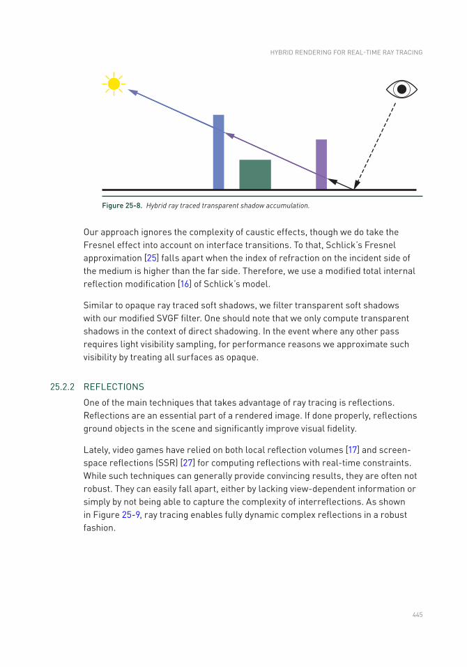
445
Figure 25-8. Hybrid ray traced transparent shadow accumulation.
Our approach ignores the complexity of caustic effects, though we do take the Fresnel effect into account on interface transitions. To that, Schlick’s Fresnel approximation [25] falls apart when the index of refraction on the incident side of the medium is higher than the far side. Therefore, we use a modified total internal reflection modification [16] of Schlick’s model.
Similar to opaque ray traced soft shadows, we filter transparent soft shadows with our modified SVGF filter. One should note that we only compute transparent shadows in the context of direct shadowing. In the event where any other pass requires light visibility sampling, for performance reasons we approximate such visibility by treating all surfaces as opaque.
25.2.2 REFLECTIONS
One of the main techniques that takes advantage of ray tracing is reflections. Reflections are an essential part of a rendered image. If done properly, reflections ground objects in the scene and significantly improve visual fidelity.
Lately, video games have relied on both local reflection volumes [17] and screen- space reflections (SSR) [27] for computing reflections with real-time constraints. While such techniques can generally provide convincing results, they are often not robust. They can easily fall apart, either by lacking view-dependent information or simply by not being able to capture the complexity of interreflections. As shown in Figure 25-9, ray tracing enables fully dynamic complex reflections in a robust fashion.
HYBRID RENDERING FOR REAL- TIME RAY TRACING
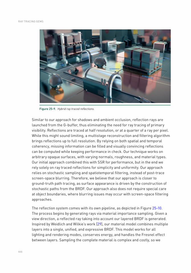
446
Figure 25-9. Hybrid ray traced reflections.
Similar to our approach for shadows and ambient occlusion, reflection rays are launched from the G-buffer, thus eliminating the need for ray tracing of primary visibility. Reflections are traced at half resolution, or at a quarter of a ray per pixel. While this might sound limiting, a multistage reconstruction and filtering algorithm brings reflections up to full resolution. By relying on both spatial and temporal coherency, missing information can be filled and visually convincing reflections can be computed while keeping performance in check. Our technique works on arbitrary opaque surfaces, with varying normals, roughness, and material types. Our initial approach combined this with SSR for performance, but in the end we rely solely on ray traced reflections for simplicity and uniformity. Our approach relies on stochastic sampling and spatiotemporal filtering, instead of post-trace screen-space blurring. Therefore, we believe that our approach is closer to ground-truth path tracing, as surface appearance is driven by the construction of stochastic paths from the BRDF. Our approach also does not require special care at object boundaries, where blurring issues may occur with screen-space filtering approaches.
The reflection system comes with its own pipeline, as depicted in Figure 25-10. The process begins by generating rays via material importance sampling. Given a view direction, a reflected ray taking into account our layered BRDF is generated. Inspired by Weidlich and Wilkie’s work [29], our material model combines multiple layers into a single, unified, and expressive BRDF. This model works for all lighting and rendering modes, conserves energy, and handles the Fresnel effect between layers. Sampling the complete material is complex and costly, so we
RAY TRACING GEMS
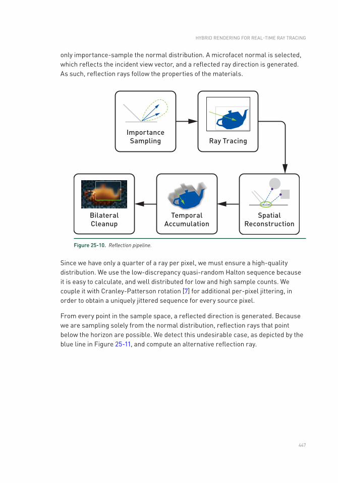
447
only importance-sample the normal distribution. A microfacet normal is selected, which reflects the incident view vector, and a reflected ray direction is generated. As such, reflection rays follow the properties of the materials.
Figure 25-10. Reflection pipeline.
Since we have only a quarter of a ray per pixel, we must ensure a high-quality distribution. We use the low-discrepancy quasi-random Halton sequence because it is easy to calculate, and well distributed for low and high sample counts. We couple it with Cranley-Patterson rotation [7] for additional per-pixel jittering, in order to obtain a uniquely jittered sequence for every source pixel.
From every point in the sample space, a reflected direction is generated. Because we are sampling solely from the normal distribution, reflection rays that point below the horizon are possible. We detect this undesirable case, as depicted by the blue line in Figure 25-11, and compute an alternative reflection ray.
HYBRID RENDERING FOR REAL- TIME RAY TRACING
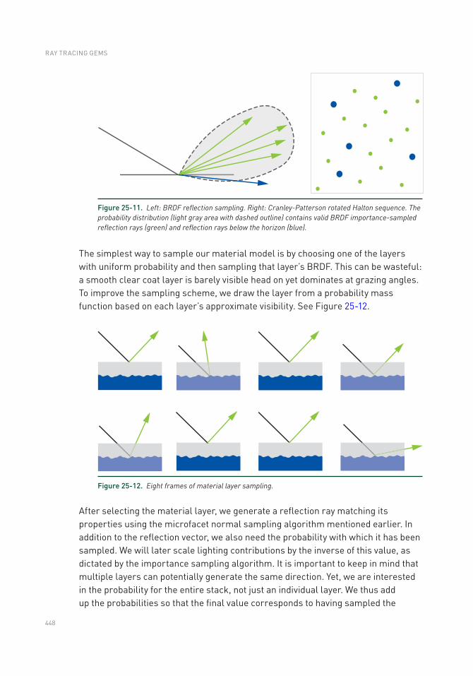
448
The simplest way to sample our material model is by choosing one of the layers with uniform probability and then sampling that layer’s BRDF. This can be wasteful: a smooth clear coat layer is barely visible head on yet dominates at grazing angles. To improve the sampling scheme, we draw the layer from a probability mass function based on each layer’s approximate visibility. See Figure 25-12.
Figure 25-11. Left: BRDF reflection sampling. Right: Cranley-Patterson rotated Halton sequence. The probability distribution (light gray area with dashed outline) contains valid BRDF importance-sampled reflection rays (green) and reflection rays below the horizon (blue).
Figure 25-12. Eight frames of material layer sampling.
After selecting the material layer, we generate a reflection ray matching its properties using the microfacet normal sampling algorithm mentioned earlier. In addition to the reflection vector, we also need the probability with which it has been sampled. We will later scale lighting contributions by the inverse of this value, as dictated by the importance sampling algorithm. It is important to keep in mind that multiple layers can potentially generate the same direction. Yet, we are interested in the probability for the entire stack, not just an individual layer. We thus add up the probabilities so that the final value corresponds to having sampled the
RAY TRACING GEMS
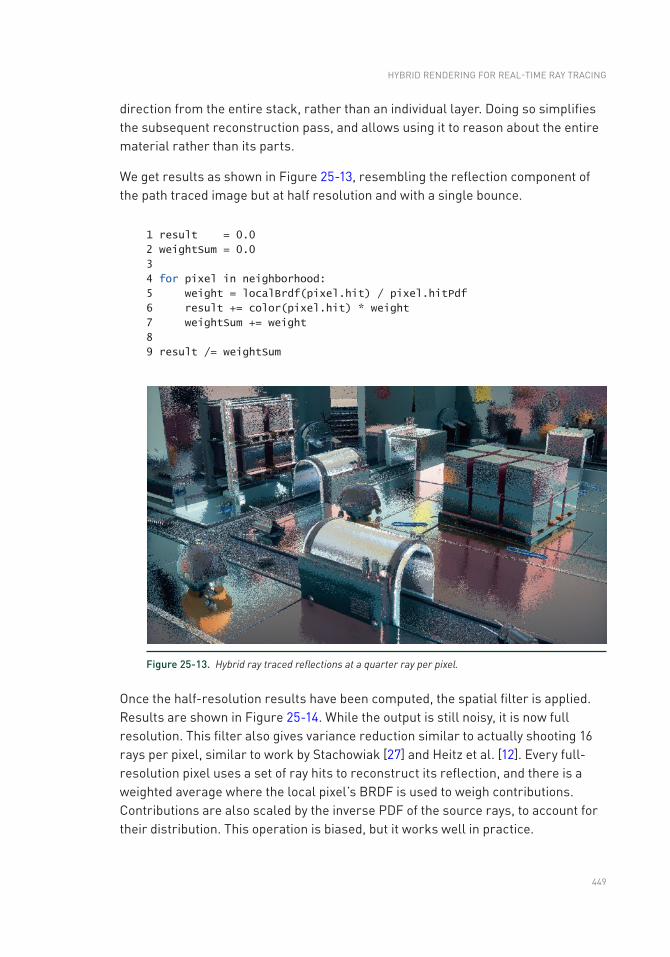
449
direction from the entire stack, rather than an individual layer. Doing so simplifies the subsequent reconstruction pass, and allows using it to reason about the entire material rather than its parts.
We get results as shown in Figure 25-13, resembling the reflection component of the path traced image but at half resolution and with a single bounce.
1 result = 0.0
2 weightSum = 0.0
3
4 for pixel in neighborhood:
5 weight = localBrdf(pixel.hit) / pixel.hitPdf
6 result += color(pixel.hit) * weight
7 weightSum += weight
8
9 result /= weightSum
Figure 25-13. Hybrid ray traced reflections at a quarter ray per pixel.
Once the half-resolution results have been computed, the spatial filter is applied. Results are shown in Figure 25-14. While the output is still noisy, it is now full resolution. This filter also gives variance reduction similar to actually shooting 16 rays per pixel, similar to work by Stachowiak [27] and Heitz et al. [12]. Every full-resolution pixel uses a set of ray hits to reconstruct its reflection, and there is a weighted average where the local pixel’s BRDF is used to weigh contributions. Contributions are also scaled by the inverse PDF of the source rays, to account for their distribution. This operation is biased, but it works well in practice.
HYBRID RENDERING FOR REAL- TIME RAY TRACING
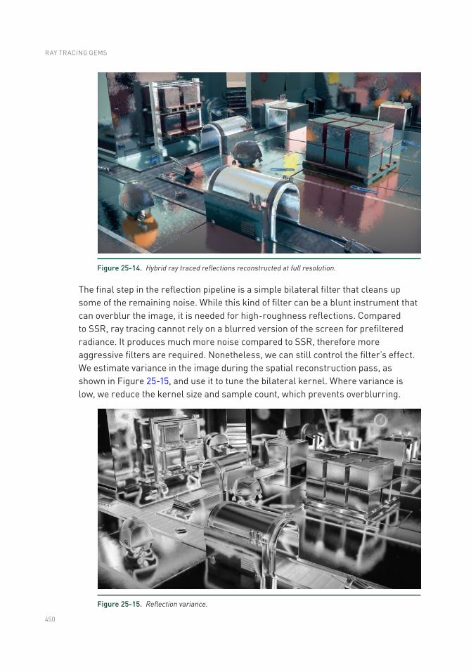
450
The final step in the reflection pipeline is a simple bilateral filter that cleans up some of the remaining noise. While this kind of filter can be a blunt instrument that can overblur the image, it is needed for high-roughness reflections. Compared to SSR, ray tracing cannot rely on a blurred version of the screen for prefiltered radiance. It produces much more noise compared to SSR, therefore more aggressive filters are required. Nonetheless, we can still control the filter’s effect. We estimate variance in the image during the spatial reconstruction pass, as shown in Figure 25-15, and use it to tune the bilateral kernel. Where variance is low, we reduce the kernel size and sample count, which prevents overblurring.
Figure 25-14. Hybrid ray traced reflections reconstructed at full resolution.
Figure 25-15. Reflection variance.
RAY TRACING GEMS
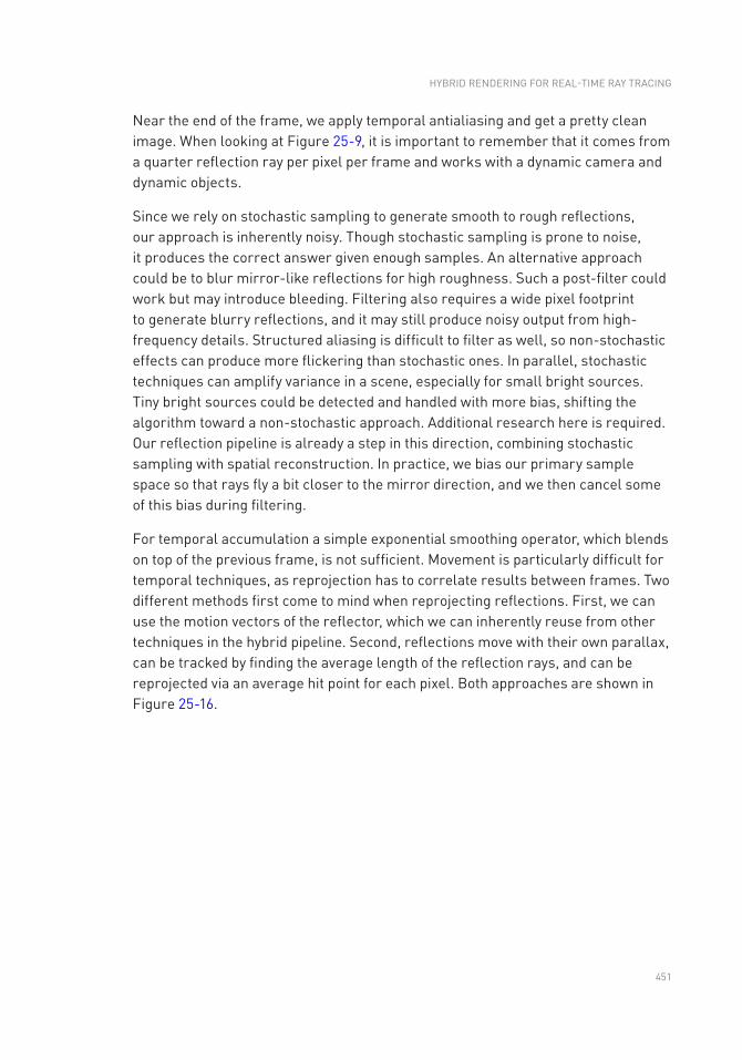
451
Near the end of the frame, we apply temporal antialiasing and get a pretty clean image. When looking at Figure 25-9, it is important to remember that it comes from a quarter reflection ray per pixel per frame and works with a dynamic camera and dynamic objects.
Since we rely on stochastic sampling to generate smooth to rough reflections, our approach is inherently noisy. Though stochastic sampling is prone to noise, it produces the correct answer given enough samples. An alternative approach could be to blur mirror-like reflections for high roughness. Such a post-filter could work but may introduce bleeding. Filtering also requires a wide pixel footprint to generate blurry reflections, and it may still produce noisy output from high-frequency details. Structured aliasing is difficult to filter as well, so non-stochastic effects can produce more flickering than stochastic ones. In parallel, stochastic techniques can amplify variance in a scene, especially for small bright sources. Tiny bright sources could be detected and handled with more bias, shifting the algorithm toward a non-stochastic approach. Additional research here is required. Our reflection pipeline is already a step in this direction, combining stochastic sampling with spatial reconstruction. In practice, we bias our primary sample space so that rays fly a bit closer to the mirror direction, and we then cancel some of this bias during filtering.
For temporal accumulation a simple exponential smoothing operator, which blends on top of the previous frame, is not sufficient. Movement is particularly difficult for temporal techniques, as reprojection has to correlate results between frames. Two different methods first come to mind when reprojecting reflections. First, we can use the motion vectors of the reflector, which we can inherently reuse from other techniques in the hybrid pipeline. Second, reflections move with their own parallax, can be tracked by finding the average length of the reflection rays, and can be reprojected via an average hit point for each pixel. Both approaches are shown in Figure 25-16.
HYBRID RENDERING FOR REAL- TIME RAY TRACING
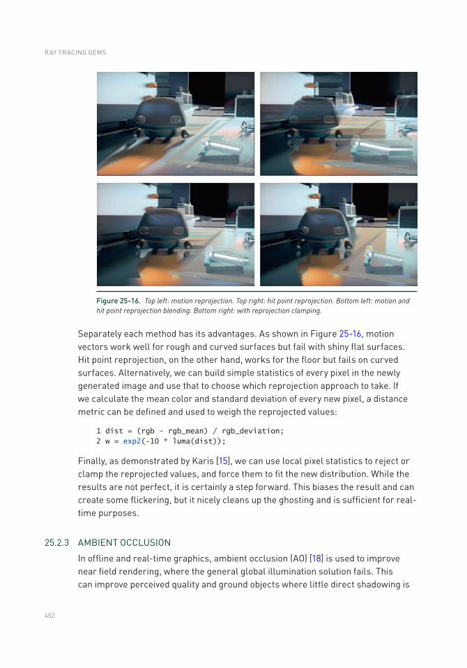
452
Separately each method has its advantages. As shown in Figure 25-16, motion vectors work well for rough and curved surfaces but fail with shiny flat surfaces. Hit point reprojection, on the other hand, works for the floor but fails on curved surfaces. Alternatively, we can build simple statistics of every pixel in the newly generated image and use that to choose which reprojection approach to take. If we calculate the mean color and standard deviation of every new pixel, a distance metric can be defined and used to weigh the reprojected values:
1 dist = (rgb - rgb_mean) / rgb_deviation;
2 w = exp2(-10 * luma(dist));
Finally, as demonstrated by Karis [15], we can use local pixel statistics to reject or clamp the reprojected values, and force them to fit the new distribution. While the results are not perfect, it is certainly a step forward. This biases the result and can create some flickering, but it nicely cleans up the ghosting and is sufficient for real-time purposes.
25.2.3 AMBIENT OCCLUSION
In offline and real-time graphics, ambient occlusion (AO) [18] is used to improve near field rendering, where the general global illumination solution fails. This can improve perceived quality and ground objects where little direct shadowing is
Figure 25-16. Top left: motion reprojection. Top right: hit point reprojection. Bottom left: motion and hit point reprojection blending. Bottom right: with reprojection clamping.
RAY TRACING GEMS
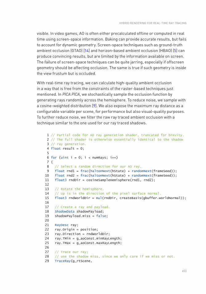
453
visible. In video games, AO is often either precalculated offline or computed in real time using screen- space information. Baking can provide accurate results, but fails to account for dynamic geometry. Screen-space techniques such as ground-truth ambient occlusion (GTAO) [14] and horizon-based ambient occlusion (HBAO) [5] can produce convincing results, but are limited by the information available on screen. The failure of screen-space techniques can be quite jarring, especially if offscreen geometry should be affecting occlusion. The same is true if such geometry is inside the view frustum but is occluded.
With real-time ray tracing, we can calculate high-quality ambient occlusion in a way that is free from the constraints of the raster-based techniques just mentioned. In PICA PICA, we stochastically sample the occlusion function by generating rays randomly across the hemisphere. To reduce noise, we sample with a cosine-weighted distribution [9]. We also expose the maximum ray distance as a configurable variable per scene, for performance but also visual-quality purposes. To further reduce noise, we filter the raw ray traced ambient occlusion with a technique similar to the one used for our ray traced shadows.
1 // Partial code for AO ray generation shader, truncated for brevity.
2 // The full shader is otherwise essentially identical to the shadow
3 // ray generation.
4 float result = 0;
5
6 for (uint i = 0; i < numRays; i++)
7
8 // Select a random direction for our AO ray.
9 float rnd1 = frac(haltonNext(hState) + randomNext(frameSeed));
10 float rnd2 = frac(haltonNext(hState) + randomNext(frameSeed));
11 float3 rndDir = cosineSampleHemisphere(rnd1, rnd2);
12
13 // Rotate the hemisphere.
14 // Up is in the direction of the pixel surface normal.
15 float3 rndWorldDir = mul(rndDir, createBasis(gbuffer.worldNormal));
16
17 // Create a ray and payload.
18 ShadowData shadowPayload;
19 shadowPayload.miss = false;
20
21 RayDesc ray;
22 ray.Origin = position;
23 ray.Direction = rndWorldDir;
24 ray.TMin = g_aoConst.minRayLength;
25 ray.TMax = g_aoConst.maxRayLength;
26
27 // Trace our ray;
28 // use the shadow miss, since we only care if we miss or not.
29 TraceRay(g_rtScene,
HYBRID RENDERING FOR REAL- TIME RAY TRACING
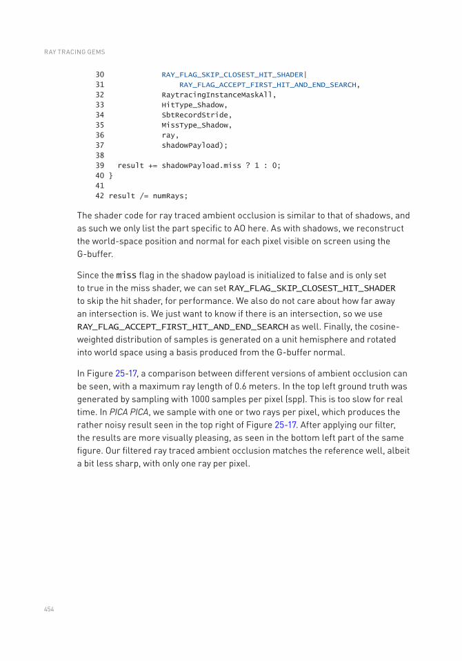
454
30 RAY_FLAG_SKIP_CLOSEST_HIT_SHADER|
31 RAY_FLAG_ACCEPT_FIRST_HIT_AND_END_SEARCH,
32 RaytracingInstanceMaskAll,
33 HitType_Shadow,
34 SbtRecordStride,
35 MissType_Shadow,
36 ray,
37 shadowPayload);
38
39 result += shadowPayload.miss ? 1 : 0;
40
41
42 result /= numRays;
The shader code for ray traced ambient occlusion is similar to that of shadows, and as such we only list the part specific to AO here. As with shadows, we reconstruct the world-space position and normal for each pixel visible on screen using the G-buffer.
Since the miss flag in the shadow payload is initialized to false and is only set to true in the miss shader, we can set RAY_FLAG_SKIP_CLOSEST_HIT_SHADER to skip the hit shader, for performance. We also do not care about how far away an intersection is. We just want to know if there is an intersection, so we use RAY_FLAG_ACCEPT_FIRST_HIT_AND_END_SEARCH as well. Finally, the cosine-weighted distribution of samples is generated on a unit hemisphere and rotated into world space using a basis produced from the G-buffer normal.
In Figure 25-17, a comparison between different versions of ambient occlusion can be seen, with a maximum ray length of 0.6 meters. In the top left ground truth was generated by sampling with 1000 samples per pixel (spp). This is too slow for real time. In PICA PICA, we sample with one or two rays per pixel, which produces the rather noisy result seen in the top right of Figure 25-17. After applying our filter, the results are more visually pleasing, as seen in the bottom left part of the same figure. Our filtered ray traced ambient occlusion matches the reference well, albeit a bit less sharp, with only one ray per pixel.
RAY TRACING GEMS
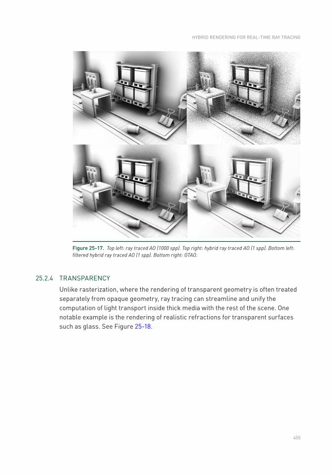
455
25.2.4 TRANSPARENCY
Unlike rasterization, where the rendering of transparent geometry is often treated separately from opaque geometry, ray tracing can streamline and unify the computation of light transport inside thick media with the rest of the scene. One notable example is the rendering of realistic refractions for transparent surfaces such as glass. See Figure 25- 18.
Figure 25-17. Top left: ray traced AO (1000 spp). Top right: hybrid ray traced AO (1 spp). Bottom left: filtered hybrid ray traced AO (1 spp). Bottom right: GTAO.
HYBRID RENDERING FOR REAL- TIME RAY TRACING
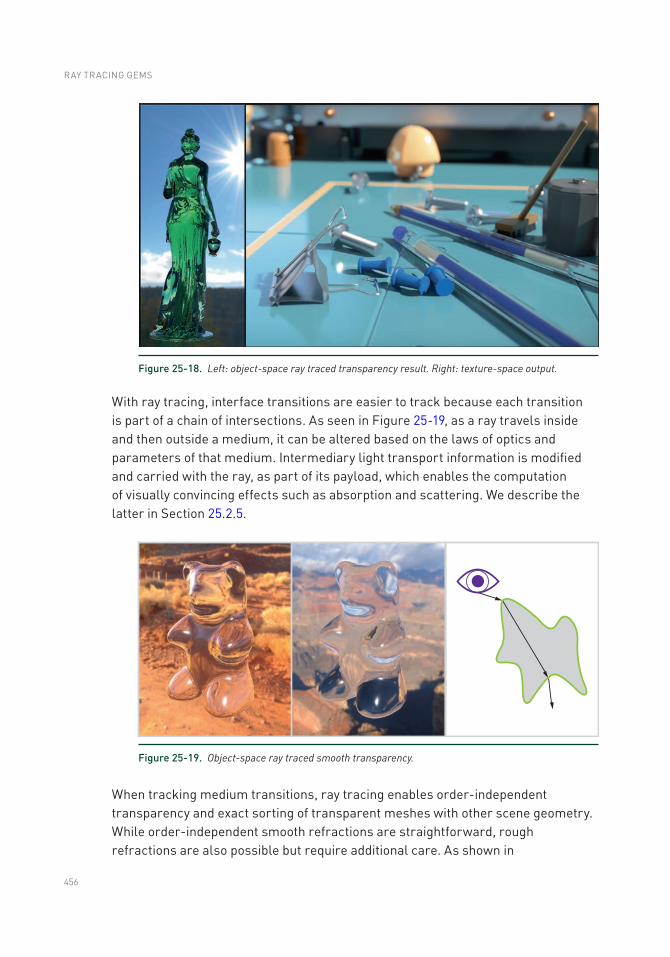
456
With ray tracing, interface transitions are easier to track because each transition is part of a chain of intersections. As seen in Figure 25-19, as a ray travels inside and then outside a medium, it can be altered based on the laws of optics and parameters of that medium. Intermediary light transport information is modified and carried with the ray, as part of its payload, which enables the computation of visually convincing effects such as absorption and scattering. We describe the latter in Section 25.2.5.
Figure 25-18. Left: object-space ray traced transparency result. Right: texture- space output.
Figure 25-19. Object-space ray traced smooth transparency.
When tracking medium transitions, ray tracing enables order-independent transparency and exact sorting of transparent meshes with other scene geometry. While order-independent smooth refractions are straightforward, rough refractions are also possible but require additional care. As shown in
RAY TRACING GEMS
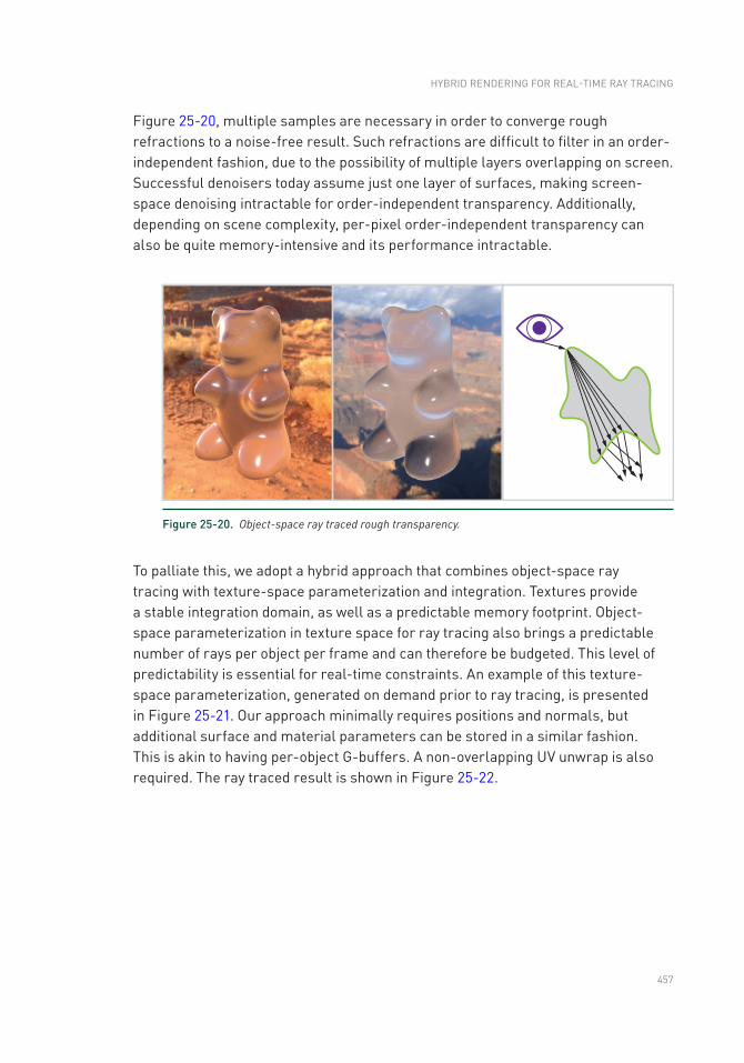
457
Figure 25-20, multiple samples are necessary in order to converge rough refractions to a noise-free result. Such refractions are difficult to filter in an order-independent fashion, due to the possibility of multiple layers overlapping on screen. Successful denoisers today assume just one layer of surfaces, making screen-space denoising intractable for order-independent transparency. Additionally, depending on scene complexity, per-pixel order- independent transparency can also be quite memory-intensive and its performance intractable.
Figure 25-20. Object-space ray traced rough transparency.
To palliate this, we adopt a hybrid approach that combines object-space ray tracing with texture-space parameterization and integration. Textures provide a stable integration domain, as well as a predictable memory footprint. Object-space parameterization in texture space for ray tracing also brings a predictable number of rays per object per frame and can therefore be budgeted. This level of predictability is essential for real-time constraints. An example of this texture-space parameterization, generated on demand prior to ray tracing, is presented in Figure 25-21. Our approach minimally requires positions and normals, but additional surface and material parameters can be stored in a similar fashion. This is akin to having per-object G-buffers. A non-overlapping UV unwrap is also required. The ray traced result is shown in Figure 25-22.
HYBRID RENDERING FOR REAL- TIME RAY TRACING
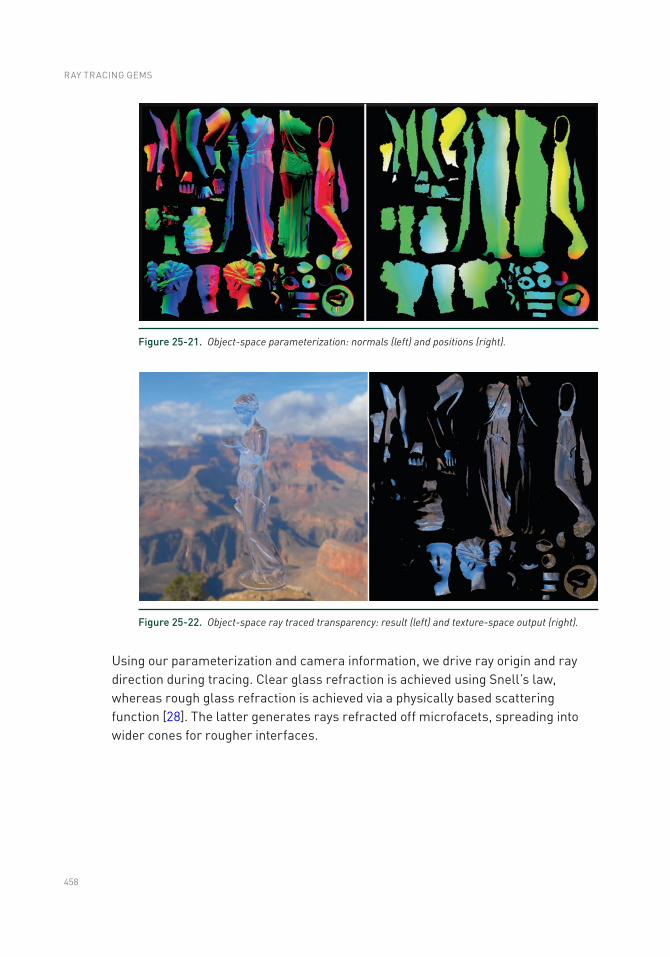
458
Using our parameterization and camera information, we drive ray origin and ray direction during tracing. Clear glass refraction is achieved using Snell’s law, whereas rough glass refraction is achieved via a physically based scattering function [28]. The latter generates rays refracted off microfacets, spreading into wider cones for rougher interfaces.
Figure 25-21. Object-space parameterization: normals (left) and positions (right).
Figure 25-22. Object-space ray traced transparency: result (left) and texture-space output (right).
RAY TRACING GEMS
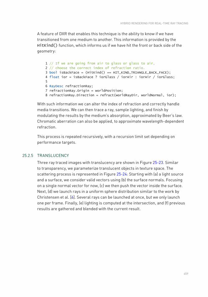
459
A feature of DXR that enables this technique is the ability to know if we have transitioned from one medium to another. This information is provided by the HitKind() function, which informs us if we have hit the front or back side of the geometry:
1 // If we are going from air to glass or glass to air,
2 // choose the correct index of refraction ratio.
3 bool isBackFace = (HitKind() == HIT_KIND_TRIANGLE_BACK_FACE);
4 float ior = isBackFace ? iorGlass / iorAir : iorAir / iorGlass;
5
6 RayDesc refractionRay;
7 refractionRay.Origin = worldPosition;
8 refractionRay.Direction = refract(worldRayDir, worldNormal, ior);
With such information we can alter the index of refraction and correctly handle media transitions. We can then trace a ray, sample lighting, and finish by modulating the results by the medium’s absorption, approximated by Beer’s law. Chromatic aberration can also be applied, to approximate wavelength-dependent refraction.
This process is repeated recursively, with a recursion limit set depending on performance targets.
25.2.5 TRANSLUCENCY
Three ray traced images with translucency are shown in Figure 25-23. Similar to transparency, we parameterize translucent objects in texture space. The scattering process is represented in Figure 25-24: Starting with (a) a light source and a surface, we consider valid vectors using (b) the surface normals. Focusing on a single normal vector for now, (c) we then push the vector inside the surface. Next, (d) we launch rays in a uniform sphere distribution similar to the work by Christensen et al. [6]. Several rays can be launched at once, but we only launch one per frame. Finally, (e) lighting is computed at the intersection, and (f) previous results are gathered and blended with the current result.
HYBRID RENDERING FOR REAL- TIME RAY TRACING
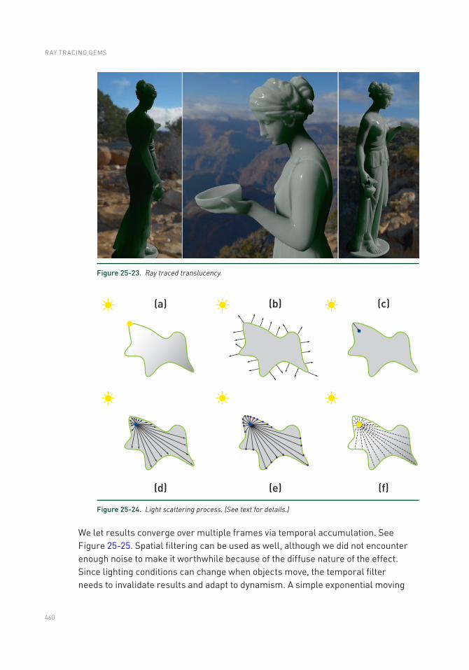
460
We let results converge over multiple frames via temporal accumulation. See Figure 25-25. Spatial filtering can be used as well, although we did not encounter enough noise to make it worthwhile because of the diffuse nature of the effect. Since lighting conditions can change when objects move, the temporal filter needs to invalidate results and adapt to dynamism. A simple exponential moving
Figure 25-23. Ray traced translucency.
Figure 25-24. Light scattering process. (See text for details.)
RAY TRACING GEMS
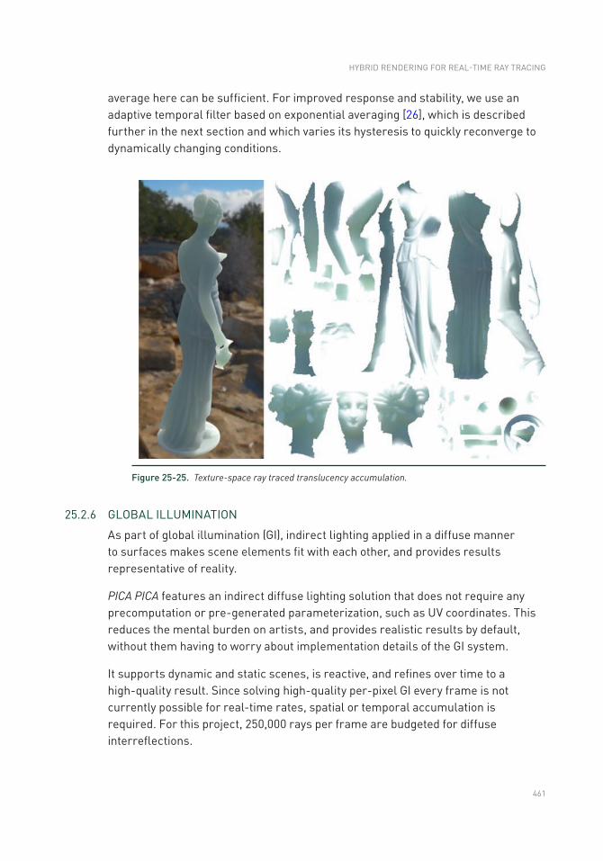
461
average here can be sufficient. For improved response and stability, we use an adaptive temporal filter based on exponential averaging [26], which is described further in the next section and which varies its hysteresis to quickly reconverge to dynamically changing conditions.
Figure 25-25. Texture-space ray traced translucency accumulation.
25.2.6 GLOBAL ILLUMINATION
As part of global illumination (GI), indirect lighting applied in a diffuse manner to surfaces makes scene elements fit with each other, and provides results representative of reality.
PICA PICA features an indirect diffuse lighting solution that does not require any precomputation or pre-generated parameterization, such as UV coordinates. This reduces the mental burden on artists, and provides realistic results by default, without them having to worry about implementation details of the GI system.
It supports dynamic and static scenes, is reactive, and refines over time to a high- quality result. Since solving high-quality per-pixel GI every frame is not currently possible for real-time rates, spatial or temporal accumulation is required. For this project, 250,000 rays per frame are budgeted for diffuse interreflections.
HYBRID RENDERING FOR REAL- TIME RAY TRACING
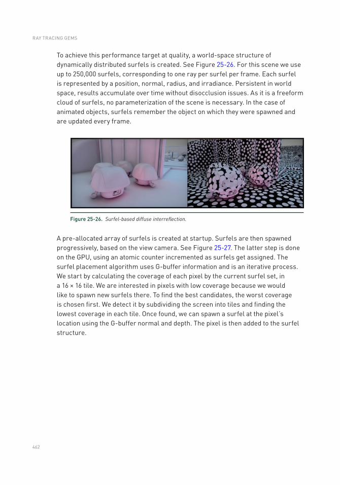
462
To achieve this performance target at quality, a world-space structure of dynamically distributed surfels is created. See Figure 25-26. For this scene we use up to 250,000 surfels, corresponding to one ray per surfel per frame. Each surfel is represented by a position, normal, radius, and irradiance. Persistent in world space, results accumulate over time without disocclusion issues. As it is a freeform cloud of surfels, no parameterization of the scene is necessary. In the case of animated objects, surfels remember the object on which they were spawned and are updated every frame.
Figure 25-26. Surfel-based diffuse interreflection.
A pre-allocated array of surfels is created at startup. Surfels are then spawned progressively, based on the view camera. See Figure 25-27. The latter step is done on the GPU, using an atomic counter incremented as surfels get assigned. The surfel placement algorithm uses G-buffer information and is an iterative process. We start by calculating the coverage of each pixel by the current surfel set, in a 16 × 16 tile. We are interested in pixels with low coverage because we would like to spawn new surfels there. To find the best candidates, the worst coverage is chosen first. We detect it by subdividing the screen into tiles and finding the lowest coverage in each tile. Once found, we can spawn a surfel at the pixel’s location using the G-buffer normal and depth. The pixel is then added to the surfel structure.
RAY TRACING GEMS
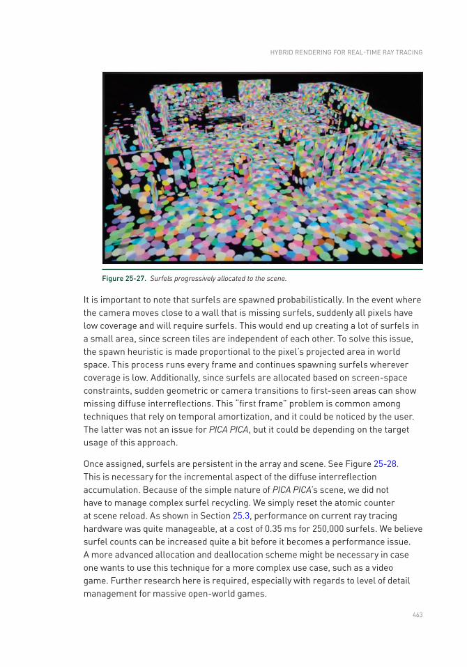
463
It is important to note that surfels are spawned probabilistically. In the event where the camera moves close to a wall that is missing surfels, suddenly all pixels have low coverage and will require surfels. This would end up creating a lot of surfels in a small area, since screen tiles are independent of each other. To solve this issue, the spawn heuristic is made proportional to the pixel’s projected area in world space. This process runs every frame and continues spawning surfels wherever coverage is low. Additionally, since surfels are allocated based on screen-space constraints, sudden geometric or camera transitions to first-seen areas can show missing diffuse interreflections. This “first frame” problem is common among techniques that rely on temporal amortization, and it could be noticed by the user. The latter was not an issue for PICA PICA, but it could be depending on the target usage of this approach.
Once assigned, surfels are persistent in the array and scene. See Figure 25-28. This is necessary for the incremental aspect of the diffuse interreflection accumulation. Because of the simple nature of PICA PICA’s scene, we did not have to manage complex surfel recycling. We simply reset the atomic counter at scene reload. As shown in Section 25.3, performance on current ray tracing hardware was quite manageable, at a cost of 0.35 ms for 250,000 surfels. We believe surfel counts can be increased quite a bit before it becomes a performance issue. A more advanced allocation and deallocation scheme might be necessary in case one wants to use this technique for a more complex use case, such as a video game. Further research here is required, especially with regards to level of detail management for massive open-world games.
Figure 25-27. Surfels progressively allocated to the scene.
HYBRID RENDERING FOR REAL- TIME RAY TRACING
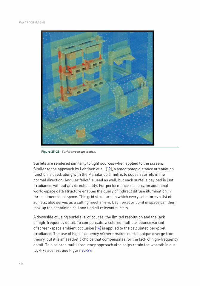
464
Surfels are rendered similarly to light sources when applied to the screen. Similar to the approach by Lehtinen et al. [19], a smoothstep distance attenuation function is used, along with the Mahalanobis metric to squash surfels in the normal direction. Angular falloff is used as well, but each surfel’s payload is just irradiance, without any directionality. For performance reasons, an additional world-space data structure enables the query of indirect diffuse illumination in three-dimensional space. This grid structure, in which every cell stores a list of surfels, also serves as a culling mechanism. Each pixel or point in space can then look up the containing cell and find all relevant surfels.
A downside of using surfels is, of course, the limited resolution and the lack of high- frequency detail. To compensate, a colored multiple-bounce variant of screen-space ambient occlusion [14] is applied to the calculated per-pixel irradiance. The use of high- frequency AO here makes our technique diverge from theory, but it is an aesthetic choice that compensates for the lack of high-frequency detail. This colored multi-frequency approach also helps retain the warmth in our toy-like scenes. See Figure 25-29.
Figure 25-28. Surfel screen application.
RAY TRACING GEMS
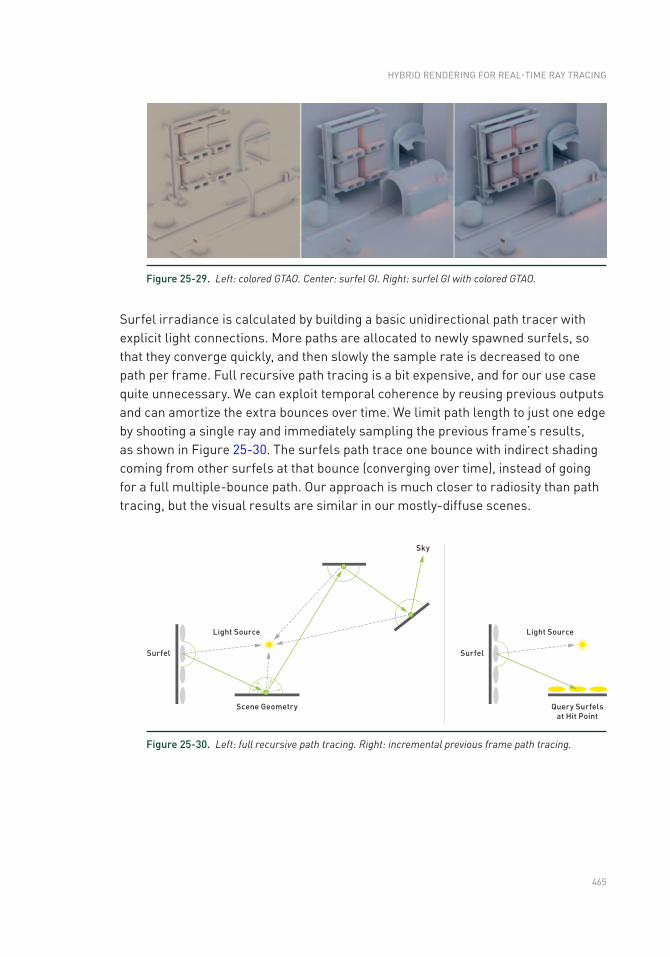
465
Surfel irradiance is calculated by building a basic unidirectional path tracer with explicit light connections. More paths are allocated to newly spawned surfels, so that they converge quickly, and then slowly the sample rate is decreased to one path per frame. Full recursive path tracing is a bit expensive, and for our use case quite unnecessary. We can exploit temporal coherence by reusing previous outputs and can amortize the extra bounces over time. We limit path length to just one edge by shooting a single ray and immediately sampling the previous frame’s results, as shown in Figure 25- 30. The surfels path trace one bounce with indirect shading coming from other surfels at that bounce (converging over time), instead of going for a full multiple-bounce path. Our approach is much closer to radiosity than path tracing, but the visual results are similar in our mostly-diffuse scenes.
Figure 25-29. Left: colored GTAO. Center: surfel GI. Right: surfel GI with colored GTAO.
Figure 25-30. Left: full recursive path tracing. Right: incremental previous frame path tracing.
HYBRID RENDERING FOR REAL- TIME RAY TRACING
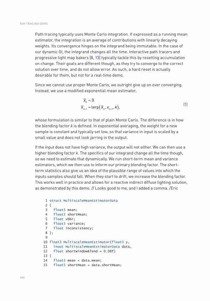
466
Path tracing typically uses Monte Carlo integration. If expressed as a running mean estimator, the integration is an average of contributions with linearly decaying weights. Its convergence hinges on the integrand being immutable. In the case of our dynamic GI, the integrand changes all the time. Interactive path tracers and progressive light map bakers [8, 13] typically tackle this by resetting accumulation on change. Their goals are different though, as they try to converge to the correct solution over time, and do not allow error. As such, a hard reset is actually desirable for them, but not for a real-time demo.
Since we cannot use proper Monte Carlo, we outright give up on ever converging. Instead, we use a modified exponential mean estimator,
( )
0
1 1lerp , , ,
0
n n n
xx x x k+ +
=
=
(1)
whose formulation is similar to that of plain Monte Carlo. The difference is in how the blending factor k is defined. In exponential averaging, the weight for a new sample is constant and typically set low, so that variance in input is scaled by a small value and does not look jarring in the output.
If the input does not have high variance, the output will not either. We can then use a higher blending factor k. The specifics of our integrand change all the time though, so we need to estimate that dynamically. We run short-term mean and variance estimators, which we then use to inform our primary blending factor. The short-term statistics also give us an idea of the plausible range of values into which the inputs samples should fall. When they start to drift, we increase the blending factor. This works well in practice and allows for a reactive indirect diffuse lighting solution, as demonstrated by this demo. // Looks good to me, and I added a comma. /Eric
1 struct MultiscaleMeanEstimatorData
2
3 float3 mean;
4 float3 shortMean;
5 float vbbr;
6 float3 variance;
7 float inconsistency;
8 ;
9
10 float3 MultiscaleMeanEstimator(float3 y,
11 inout MultiscaleMeanEstimatorData data,
12 float shortWindowBlend = 0.08f)
13
14 float3 mean = data.mean;
15 float3 shortMean = data.shortMean;
RAY TRACING GEMS
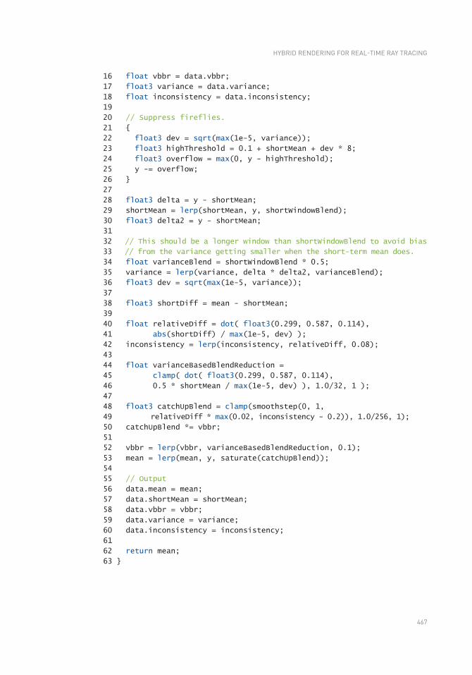
467
16 float vbbr = data.vbbr;
17 float3 variance = data.variance;
18 float inconsistency = data.inconsistency;
19
20 // Suppress fireflies.
21
22 float3 dev = sqrt(max(1e-5, variance));
23 float3 highThreshold = 0.1 + shortMean + dev * 8;
24 float3 overflow = max(0, y - highThreshold);
25 y -= overflow;
26
27
28 float3 delta = y - shortMean;
29 shortMean = lerp(shortMean, y, shortWindowBlend);
30 float3 delta2 = y - shortMean;
31
32 // This should be a longer window than shortWindowBlend to avoid bias
33 // from the variance getting smaller when the short-term mean does.
34 float varianceBlend = shortWindowBlend * 0.5;
35 variance = lerp(variance, delta * delta2, varianceBlend);
36 float3 dev = sqrt(max(1e-5, variance));
37
38 float3 shortDiff = mean - shortMean;
39
40 float relativeDiff = dot( float3(0.299, 0.587, 0.114),
41 abs(shortDiff) / max(1e-5, dev) );
42 inconsistency = lerp(inconsistency, relativeDiff, 0.08);
43
44 float varianceBasedBlendReduction =
45 clamp( dot( float3(0.299, 0.587, 0.114),
46 0.5 * shortMean / max(1e-5, dev) ), 1.0/32, 1 );
47
48 float3 catchUpBlend = clamp(smoothstep(0, 1,
49 relativeDiff * max(0.02, inconsistency - 0.2)), 1.0/256, 1);
50 catchUpBlend *= vbbr;
51
52 vbbr = lerp(vbbr, varianceBasedBlendReduction, 0.1);
53 mean = lerp(mean, y, saturate(catchUpBlend));
54
55 // Output
56 data.mean = mean;
57 data.shortMean = shortMean;
58 data.vbbr = vbbr;
59 data.variance = variance;
60 data.inconsistency = inconsistency;
61
62 return mean;
63
HYBRID RENDERING FOR REAL- TIME RAY TRACING
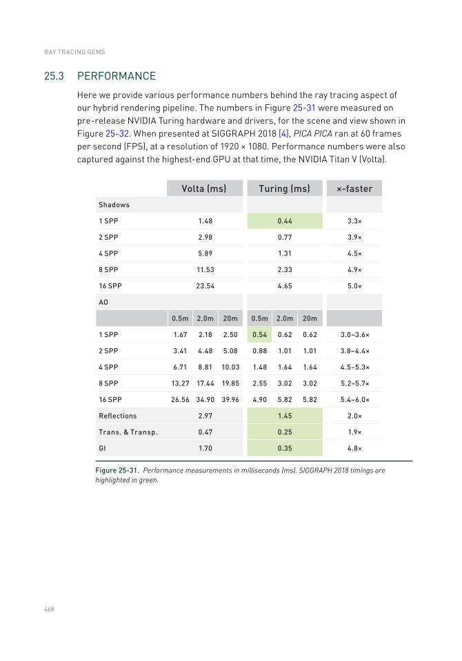
468
25.3 PERFORMANCE
Here we provide various performance numbers behind the ray tracing aspect of our hybrid rendering pipeline. The numbers in Figure 25-31 were measured on pre-release NVIDIA Turing hardware and drivers, for the scene and view shown in Figure 25-32. When presented at SIGGRAPH 2018 [4], PICA PICA ran at 60 frames per second (FPS), at a resolution of 1920 × 1080. Performance numbers were also captured against the highest-end GPU at that time, the NVIDIA Titan V (Volta).
Figure 25-31. Performance measurements in milliseconds (ms). SIGGRAPH 2018 timings are highlighted in green.
RAY TRACING GEMS
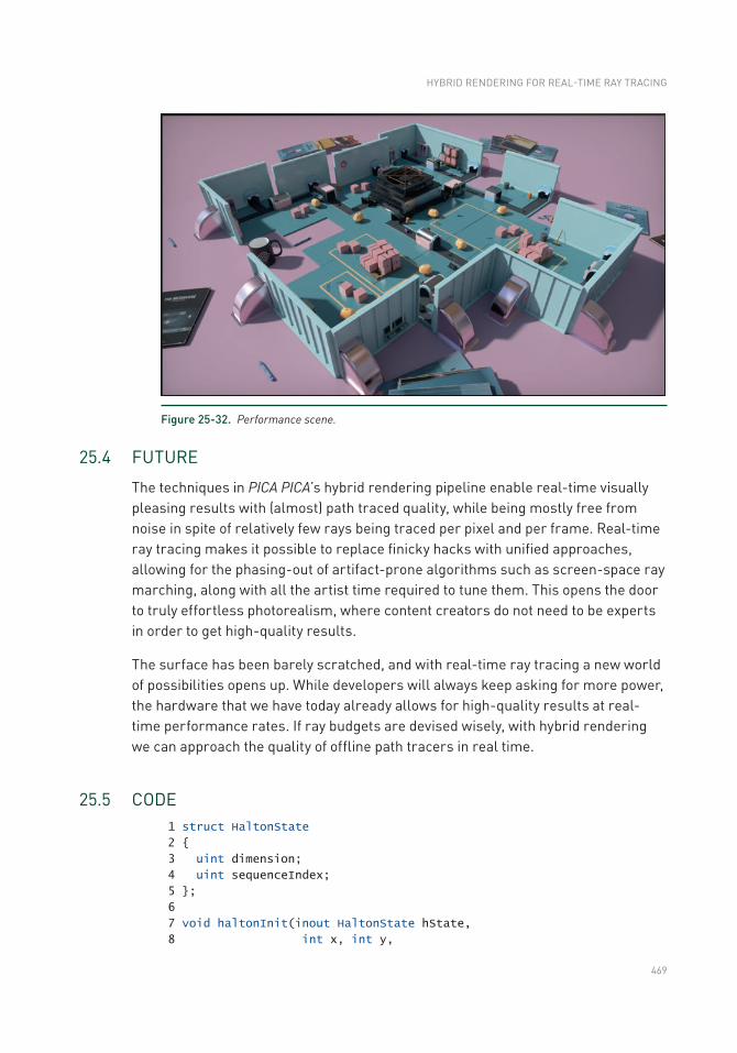
469
25.4 FUTURE
The techniques in PICA PICA’s hybrid rendering pipeline enable real-time visually pleasing results with (almost) path traced quality, while being mostly free from noise in spite of relatively few rays being traced per pixel and per frame. Real-time ray tracing makes it possible to replace finicky hacks with unified approaches, allowing for the phasing-out of artifact-prone algorithms such as screen-space ray marching, along with all the artist time required to tune them. This opens the door to truly effortless photorealism, where content creators do not need to be experts in order to get high- quality results.
The surface has been barely scratched, and with real-time ray tracing a new world of possibilities opens up. While developers will always keep asking for more power, the hardware that we have today already allows for high-quality results at real-time performance rates. If ray budgets are devised wisely, with hybrid rendering we can approach the quality of offline path tracers in real time.
25.5 CODE 1 struct HaltonState
2
3 uint dimension;
4 uint sequenceIndex;
5 ;
6
7 void haltonInit(inout HaltonState hState,
8 int x, int y,
Figure 25-32. Performance scene.
HYBRID RENDERING FOR REAL- TIME RAY TRACING
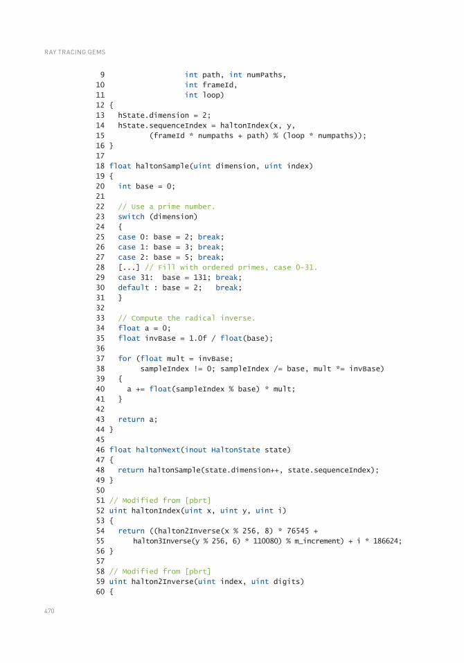
470
9 int path, int numPaths,
10 int frameId,
11 int loop)
12
13 hState.dimension = 2;
14 hState.sequenceIndex = haltonIndex(x, y,
15 (frameId * numpaths + path) % (loop * numpaths));
16
17
18 float haltonSample(uint dimension, uint index)
19
20 int base = 0;
21
22 // Use a prime number.
23 switch (dimension)
24
25 case 0: base = 2; break;
26 case 1: base = 3; break;
27 case 2: base = 5; break;
28 [...] // Fill with ordered primes, case 0-31.
29 case 31: base = 131; break;
30 default : base = 2; break;
31
32
33 // Compute the radical inverse.
34 float a = 0;
35 float invBase = 1.0f / float(base);
36
37 for (float mult = invBase;
38 sampleIndex != 0; sampleIndex /= base, mult *= invBase)
39
40 a += float(sampleIndex % base) * mult;
41
42
43 return a;
44
45
46 float haltonNext(inout HaltonState state)
47
48 return haltonSample(state.dimension++, state.sequenceIndex);
49
50
51 // Modified from [pbrt]
52 uint haltonIndex(uint x, uint y, uint i)
53
54 return ((halton2Inverse(x % 256, 8) * 76545 +
55 halton3Inverse(y % 256, 6) * 110080) % m_increment) + i * 186624;
56
57
58 // Modified from [pbrt]
59 uint halton2Inverse(uint index, uint digits)
60
RAY TRACING GEMS
471
61 index = (index << 16) | (index >> 16);
62 index = ((index & 0x00ff00ff) << 8) | ((index & 0xff00ff00) >> 8);
63 index = ((index & 0x0f0f0f0f) << 4) | ((index & 0xf0f0f0f0) >> 4);
64 index = ((index & 0x33333333) << 2) | ((index & 0xcccccccc) >> 2);
65 index = ((index & 0x55555555) << 1) | ((index & 0xaaaaaaaa) >> 1);
66 return index >> (32 - digits);
67
68
69 // Modified from [pbrt]
70 uint halton3Inverse(uint index, uint digits)
71
72 uint result = 0;
73 for (uint d = 0; d < digits; ++d)
74
75 result = result * 3 + index % 3;
76 index /= 3;
77
78 return result;
79
ACKNOWLEDGMENTS
The authors would like to thank the PICA PICA team at SEED, a technical and creative research division of Electronic Arts. We would also like to thank our friends at Frostbite and DICE, with whom we have had great discussions and collaboration as we built this hybrid rendering pipeline. Moreover, this endeavor would not have been possible without support from the folks at NVIDIA and the DirectX team at Microsoft. The authors would also like to thank Morgan McGuire for his review of this chapter, as well as Tomas Akenine-Möller and Eric Haines for their insight and support.
REFERENCES
[1] Akenine-Möller, T., Haines, E., Hoffman, N., Pesce, A., Iwanicki, M., and Hillaire, S. Real-Time Rendering, fourth ed. A K Peters/CRC Press, 2018.
[2] Andersson, J., and Barré-Brisebois, C. DirectX: Evolving Microsoft’s Graphics Platform. Microsoft Sponsored Session, Game Developers Conference, 2018.
[3] Andersson, J., and Barré-Brisebois, C. Shiny Pixels and Beyond: Real-Time Raytracing at SEED. NVIDIA Sponsored Session, Game Developers Conference, 2018.
[4] Barré-Brisebois, C., and Halén, H. PICA PICA and NVIDIA Turing. NVIDIA Sponsored Session, SIGGRAPH, 2018.
[5] Bavoil, L., Sainz, M., and Dimitrov, R. Image-Space Horizon-Based Ambient Occlusion. In ACM SIGGRAPH Talks (2008), p. 22:1.
HYBRID RENDERING FOR REAL- TIME RAY TRACING

472
[6] Christensen, P., Harker, G., Shade, J., Schubert, B., and Batali, D. Multiresolution Radiosity Caching for Global Illumination in Movies. In ACM SIGGRAPH Talks (2012), p. 47:1.
[7] Cranley, R., and Patterson, T. Randomization of Number Theoretic Methods for Multiple Integration. SIAM Journal on Numerical Analysis 13, 6 (1976), 904–914.
[8] Dean, M., and Nordwall, J. Make It Shiny: Unity’s Progressive Lightmapper and Shader Graph. Game Developers Conference, 2016.
[9] Dutré, P., Bekaert, P., and Bala, K. Advanced Global Illumination. A K Peters, 2006.
[10] EA SEED. Project PICA PICA—Real-Time Raytracing Experiment Using DXR (DirectX Raytracing). https://www.youtube.com/watch?v=LXo0WdlELJk, March 2018.
[11] Fong, J., Wrenninge, M., Kulla, C., and Habel, R. Production Volume Rendering. Production Volume Rendering, SIGGRAPH Courses, 2017.
[12] Heitz, E., Hill, S., and McGuire, M. Combining Analytic Direct Illumination and Stochastic Shadows. In Symposium on Interactive 3D Graphics and Games (2018), pp. 2:1–2:11.
[13] Hillaire, S. Real-Time Raytracing for Interactive Global Illumination Workflows in Frostbite. NVIDIA Sponsored Session, Game Developers Conference, 2018.
[14] Jiménez, J., Wu, X., Pesce, A., and Jarabo, A. Practical Real-Time Strategies for Accurate Indirect Occlusion. Physically Based Shading in Theory and Practice, SIGGRAPH Courses, 2016.
[15] Karis, B. High-Quality Temporal Supersampling. Advances in Real-Time Rendering in Games, SIGGRAPH Courses, 2014.
[16] Lagarde, S. Memo on Fresnel Equations. Blog, April 2013.
[17] Lagarde, S., and Zanuttini, A. Local Image-Based Lighting with Parallax-Corrected Cubemap. In SIGGRAPH Talks (2012), p. 36:1.
[18] Landis, H. Production-Ready Global Illumination. RenderMan in Production, SIGGRAPH Courses, 2002.
[19] Lehtinen, J., Zwicker, M., Turquin, E., Kontkanen, J., Durand, F., Sillion, F., and Aila, T. A Meshless Hierarchical Representation for Light Transport. ACM Transactions in Graphics 27, 3 (2008), 37:1–37:10.
[20] McGuire, M., and Mara, M. Phenomenological Transparency. IEEE Transactions on Visualization and Computer Graphics 23, 5 (2017), 1465–1478.
[21] Pharr, M., Jakob, W., and Humphreys, G. Physically Based Rendering: From Theory to Implementation, third ed. Morgan Kaufmann, 2016.
[22] Salvi, M. An Excursion in Temporal Supersampling. From the Lab Bench: Real-Time Rendering Advances from NVIDIA Research, Game Developers Conference, 2016.
RAY TRACING GEMS

473
[23] Sandy, M. Announcing Microsoft DirectX Raytracing! DirectX Developer Blog, https://blogs.msdn.microsoft.com/directx/2018/03/19/announcing- microsoft- directx-
raytracing/, March 2018.
[24] Schied, C., Kaplanyan, A., Wyman, C., Patney, A., Chaitanya, C. R. A., Burgess, J., Liu, S., Dachsbacher, C., Lefohn, A., and Salvi, M. Spatiotemporal Variance- Guided Filtering: Real-Time Reconstruction for Path-Traced Global Illumination. In Proceedings of High-Performance Graphics (2017), pp. 2:1–2:12.
[25] Schlick, C. An Inexpensive BRDF Model for Physically-based Rendering. Computer Graphics Forum 13, 3 (1994), 233–246.
[26] Stachowiak, T. Stochastic All The Things: Raytracing in Hybrid Real-Time Rendering. Digital Dragons Presentation, 2018.
[27] Stachowiak, T., and Uludag, Y. Stochastic Screen-Space Reflections. Advances in Real-Time Rendering, SIGGRAPH Courses, 2015.
[28] Walter, B., Marschner, S. R., Li, H., and Torrance, K. E. Microfacet Models for Refraction through Rough Surfaces. In Eurographics Symposium on Rendering (2007), pp. 195–206.
[29] Weidlich, A., and Wilkie, A. Arbitrary Layered Micro-Facet Surfaces. In GRAPHITE (2007), pp. 171–178.
Open Access This chapter is licensed under the terms of the Creative Commons Attribution-NonCommercial-NoDerivatives 4.0 International License (http://creativecommons.org/licenses/by-nc-nd/4.0/), which permits any noncommercial use, sharing, distribution and
reproduction in any medium or format, as long as you give appropriate credit to the original author(s) and the source, provide a link to the Creative Commons license and indicate if you modified the licensed material. You do not have permission under this license to share adapted material derived from this chapter or parts of it.
The images or other third party material in this chapter are included in the chapter's Creative Commons license, unless indicated otherwise in a credit line to the material. If material is not included in the chapter's Creative Commons license and your intended use is not permitted by statutory regulation or exceeds the permitted use, you will need to obtain permission directly from the copyright holder.
HYBRID RENDERING FOR REAL- TIME RAY TRACING
475© NVIDIA 2019 E. Haines, T. Akenine-Möller (eds.), Ray Tracing Gems, https://doi.org/10.1007/978-1-4842-4427-2_26
CHAPTER 26
Deferred Hybrid Path TracingThomas Willberger, Clemens Musterle, and Stephan Bergmann Enscape GmbH
ABSTRACT
We describe a hybrid rendering approach that leverages existing rasterization-based techniques and combines them with ray tracing in order to achieve real-time global illumination. We reduce the number of traced rays by trying to find an intersection in screen space and reuse information from previous frames via reprojection and filtering. Artificial lighting is stored in nodes of the spatial acceleration structure to ensure efficient memory access. Our techniques require no manual preprocessing and only a few seconds of precomputation. They were developed as a real-time rendering solution for architectural design but can be applied to other purposes as well.
26.1 OVERVIEW
Despite recent advances in GPU-accelerated ray tracing, it remains challenging to seamlessly scale ray tracing–based algorithms across a large variety of scene complexities while maintaining acceptable performance. This is especially true for scenarios (unlike games) where no artist can define to what extent and detail level ray tracing should be applied. We aim to provide global illumination on mostly static scene content without perceivable precomputation and with few assumptions about the scene.
To do so, we first render the scene to a G-buffer and then spawn rays from G-buffer pixels to evaluate the lighting. For each ray, we try to find intersections in screen space because, if successful, this is usually faster than tracing the ray in a spatial data structure. Additionally, we use fully lit pixels from the previous frame to get accumulated multiple- bounce lighting. If tracing in screen space is not successful, we continue tracing in a spatial data structure, in our case a bounding volume hierarchy (BVH), while keeping the visual quality degradation as low as possible. Figure 26-1 shows an actual image resulting from our implementation.
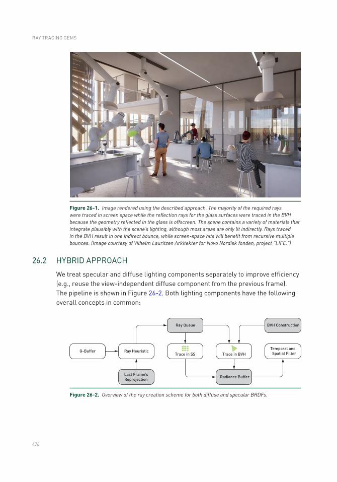
476
26.2 HYBRID APPROACH
We treat specular and diffuse lighting components separately to improve efficiency (e.g., reuse the view-independent diffuse component from the previous frame). The pipeline is shown in Figure 26-2. Both lighting components have the following overall concepts in common:
Figure 26-1. Image rendered using the described approach. The majority of the required rays were traced in screen space while the reflection rays for the glass surfaces were traced in the BVH because the geometry reflected in the glass is offscreen. The scene contains a variety of materials that integrate plausibly with the scene’s lighting, although most areas are only lit indirectly. Rays traced in the BVH result in one indirect bounce, while screen-space hits will benefit from recursive multiple bounces. (Image courtesy of Vilhelm Lauritzen Arkitekter for Novo Nordisk fonden, project “LIFE.”)
Figure 26-2. Overview of the ray creation scheme for both diffuse and specular BRDFs.
RAY TRACING GEMS
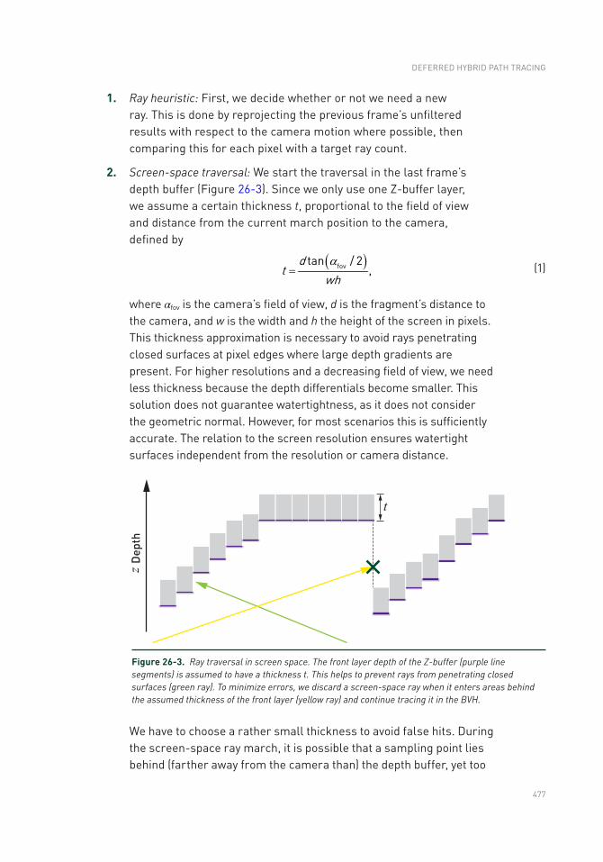
477
1. Ray heuristic: First, we decide whether or not we need a new ray. This is done by reprojecting the previous frame’s unfiltered results with respect to the camera motion where possible, then comparing this for each pixel with a target ray count.
2. Screen-space traversal: We start the traversal in the last frame’s depth buffer (Figure 26-3). Since we only use one Z-buffer layer, we assume a certain thickness t, proportional to the field of view and distance from the current march position to the camera, defined by
( )dt
whfovtan / 2
,a
= (1)
where αfov is the camera’s field of view, d is the fragment’s distance to the camera, and w is the width and h the height of the screen in pixels. This thickness approximation is necessary to avoid rays penetrating closed surfaces at pixel edges where large depth gradients are present. For higher resolutions and a decreasing field of view, we need less thickness because the depth differentials become smaller. This solution does not guarantee watertightness, as it does not consider the geometric normal. However, for most scenarios this is sufficiently accurate. The relation to the screen resolution ensures watertight surfaces independent from the resolution or camera distance.
We have to choose a rather small thickness to avoid false hits. During the screen- space ray march, it is possible that a sampling point lies behind (farther away from the camera than) the depth buffer, yet too
Figure 26-3. Ray traversal in screen space. The front layer depth of the Z-buffer (purple line segments) is assumed to have a thickness t. This helps to prevent rays from penetrating closed surfaces (green ray). To minimize errors, we discard a screen-space ray when it enters areas behind the assumed thickness of the front layer (yellow ray) and continue tracing it in the BVH.
DEFERRED HYBRID PATH TRACING
478
far away to be within the accepted thickness range. We lack reliable information about the occluded geometry. Therefore, the ray is not counted as being a hit, so we immediately stop the screen-space traversal. We classify such a ray as no-hit because we cannot be sure if there is more geometry that is not present in screen space.
Reading from the last frame’s irradiance result, however, is inaccurate because some of the lighting information is view-dependent. To solve this, we store a buffer without the view-dependent components (specular) or alpha-blended geometry. This introduces an energy loss, which is currently compensated by a constant factor. The ray march result is written into a buffer of ray lengths. Then, we reconstruct the fetch position in the last frame’s buffer for a subsequent pass to leverage the texture cache usage during traversal.
3. BVH traversal: We continue the ray traversal in our BVH, at the position where our screen space cast ends, and evaluate a radiance value. In the case of no hit, we write a skybox fetch into the accumulation buffer, which stores the radiance sum of all ray casts. This fetch can be slightly biased to reduce variance by reading from a filtered mip level depending on the estimated lobe size.
4. Filtering: Before compositing the traversal result, we employ a spatial filter followed by a temporal filter.
26.3 BVH TRAVERSAL
The range of complexity of our customers’ scenes is rather large. To make sure that we can handle even large scenes with a reasonable impact on performance and memory requirements, our BVH does not contain all the scene geometry. This means that at any given time only a subset of the whole scene is included in the BVH. This subset is usually centered around the camera, which is achieved by continuously and asynchronously constructing the BVH, depending on the camera’s position, and results in geometry being removed and added while the camera moves in the scene. Due to the temporal caching of various radiance buffers, the geometric change is mostly smooth. However, on some surfaces that lack a stable temporal accumulation, like alpha-blended geometry, it can be noticeable. The challenge is to include only the visually most relevant objects within our performance budget in the BVH.
RAY TRACING GEMS
479
26.3.1 GEOMETRY SELECTION
To select the relevant geometry, the total scene geometry has to be divided into meaningful parts that can be independently selected for inclusion in the BVH. This partition can be done at the hierarchy level of objects, but it was apparent that objects with a high triangle count needed to be subdivided further, so we included an automatic subdivision. We define a score function per object that describes the visual importance j,
aj pd 2
,= (2)
where a is the projected surface area and d is the object’s distance to the camera, making the first term comparable to the object’s subtended solid angle as seen from the camera. The second term p is an object-specific importance factor that is greater than one for emissive surfaces because their absence will have a larger visual impact than non-emissive surfaces, for which p = 1.
All objects are ordered by their visual importance j. Depending on the desired quality level, we define a total cost budget that is allowed to ensure the desired frame rate. We include the objects with the highest importance score until that budget is reached. Beside the polygon count, the cost is also multiplied by an efficiency factor that tries to predict how many axis-aligned bounding box tests are necessary to successfully intersect a primitive or leave the model’s bounding box. For this factor, we use a heuristic based on the number of shared vertices in the triangle meshes. This heuristic is motivated by our experience that if triangles rarely share vertices (as in the case of vegetation), traversal performance is usually less efficient.
We end up with BVH trees with less than 10 MB that are uploaded from CPU to GPU in a couple of milliseconds. This delay can usually be hidden by double buffering.
26.3.2 VERTEX PREPROCESSING
For each vertex in the BVH, we precompute a single irradiance value during BVH construction. This is done to avoid having to continue tracing the BVH after the first hit, which would be expensive because the rays will be increasingly incoherent and thus incur higher computation and memory access cost. For each vertex in the BVH, we compute an irradiance value using all the lights whose area of influence include the vertex. To test the visibility, we trace a shadow ray for each vertex-light combination. When these precomputed irradiance values are used in our
DEFERRED HYBRID PATH TRACING
480
lighting computation when tracing, a path from a G-buffer pixel in the BVH has the following consequences/simplifications:
> We will include paths with two bounces in our lighting calculation when tracing within the BVH, although it is only a rather coarse approximation.
> We simplify the shading in the BVH traversal, to the extent that we only include diffuse shading components, and the irradiance at each point on the triangle’s surface is assumed to be a barycentric interpolation of the irradiance of the triangle’s vertices.
To avoid errors that are too perceptually noticeable due to the second simplification, we subdivide triangles where the difference between adjacent vertices’ irradiance values exceeds a pre-configured threshold.
26.3.3 SHADING
To avoid an additional access to material data or UV coordinates, we store only a single albedo value per triangle in the BVH. The texture’s albedo is therefore averaged when creating the BVH. For cutout masks, we calculate the number of visible pixels and approximate the ratio with a procedural cutout pattern, which can be cheaply evaluated in the intersection shader after the triangle/ray intersection test discards the hit. While these approximations work well for diffuse lighting, the missing material and texture information can become apparent for sharp specular reflections. Therefore, we sample the surface’s albedo texture for glossy specular reflections. This mode is optional and can be disabled to ensure higher performance in scenarios like virtual reality.
The total shading then consists of the per-vertex artificial lighting amount, the shadow mapped sunlight, and an ambient amount to compensate for missing multiple bounces, which is only applied at the last ray intersection. The ambient amount is proportional to an atmosphere skybox read (convolved with a cosine distribution) and an ambient occlusion factor. We approximate ambient occlusion by multiplying an exponential function with −d being the ray distance toward the surface and k being a scaling factor that is chosen empirically. This is a hemisphere estimation with only one sample, but it helps to reduce the ambient factor in indoor scenarios to avoid light leaking leading to an ambient factor
( )skybox vertex sun ,dka m e r r r-= + + (3)
where m is the albedo and r represents various radiance sources.
RAY TRACING GEMS
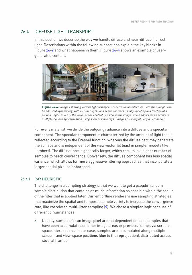
481
26.4 DIFFUSE LIGHT TRANSPORT
In this section we describe the way we handle diffuse and near-diffuse indirect light. Descriptions within the following subsections explain the key blocks in Figure 26-2 and what happens in them. Figure 26-4 shows an example of user-generated content.
For every material, we divide the outgoing radiance into a diffuse and a specular component. The specular component is characterized by the amount of light that is reflected according to the Fresnel function, whereas the diffuse part may penetrate the surface and is independent of the view vector (at least in simpler models like Lambert). The diffuse lobe is generally larger, which results in a higher number of samples to reach convergence. Conversely, the diffuse component has less spatial variance, which allows for more aggressive filtering approaches that incorporate a larger spatial pixel neighborhood.
26.4.1 RAY HEURISTIC
The challenge in a sampling strategy is that we want to get a pseudo-random sample distribution that contains as much information as possible within the radius of the filter that is applied later. Current offline renderers use sampling strategies that maximize the spatial and temporal sample variety to increase the convergence rate, like correlated multi-jitter sampling [9]. We chose a simpler logic because of different circumstances:
> Usually, samples for an image pixel are not dependent on past samples that have been accumulated on other image areas or previous frames via screen-space intersections. In our case, samples are accumulated along multiple screen- and view-space positions (due to the reprojection), distributed across several frames.
Figure 26-4. Images showing various light transport scenarios in architecture. Left: the sunlight can be adjusted dynamically, with all other lights and scene contents usually updating in a fraction of a second. Right: much of the visual scene content is visible in the image, which allows for an accurate multiple-bounce approximation using screen-space rays. (Images courtesy of Sergio Fernando.)
DEFERRED HYBRID PATH TRACING
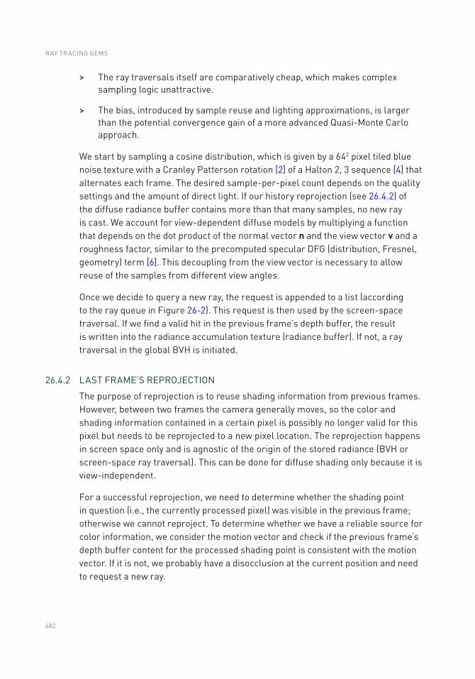
482
> The ray traversals itself are comparatively cheap, which makes complex sampling logic unattractive.
> The bias, introduced by sample reuse and lighting approximations, is larger than the potential convergence gain of a more advanced Quasi-Monte Carlo approach.
We start by sampling a cosine distribution, which is given by a 642 pixel tiled blue noise texture with a Cranley Patterson rotation [2] of a Halton 2, 3 sequence [4] that alternates each frame. The desired sample-per-pixel count depends on the quality settings and the amount of direct light. If our history reprojection (see 26.4.2) of the diffuse radiance buffer contains more than that many samples, no new ray is cast. We account for view-dependent diffuse models by multiplying a function that depends on the dot product of the normal vector n and the view vector v and a roughness factor, similar to the precomputed specular DFG (distribution, Fresnel, geometry) term [6]. This decoupling from the view vector is necessary to allow reuse of the samples from different view angles.
Once we decide to query a new ray, the request is appended to a list (according to the ray queue in Figure 26-2). This request is then used by the screen-space traversal. If we find a valid hit in the previous frame’s depth buffer, the result is written into the radiance accumulation texture (radiance buffer). If not, a ray traversal in the global BVH is initiated.
26.4.2 LAST FRAME’S REPROJECTION
The purpose of reprojection is to reuse shading information from previous frames. However, between two frames the camera generally moves, so the color and shading information contained in a certain pixel is possibly no longer valid for this pixel but needs to be reprojected to a new pixel location. The reprojection happens in screen space only and is agnostic of the origin of the stored radiance (BVH or screen-space ray traversal). This can be done for diffuse shading only because it is view-independent.
For a successful reprojection, we need to determine whether the shading point in question (i.e., the currently processed pixel) was visible in the previous frame; otherwise we cannot reproject. To determine whether we have a reliable source for color information, we consider the motion vector and check if the previous frame’s depth buffer content for the processed shading point is consistent with the motion vector. If it is not, we probably have a disocclusion at the current position and need to request a new ray.
RAY TRACING GEMS
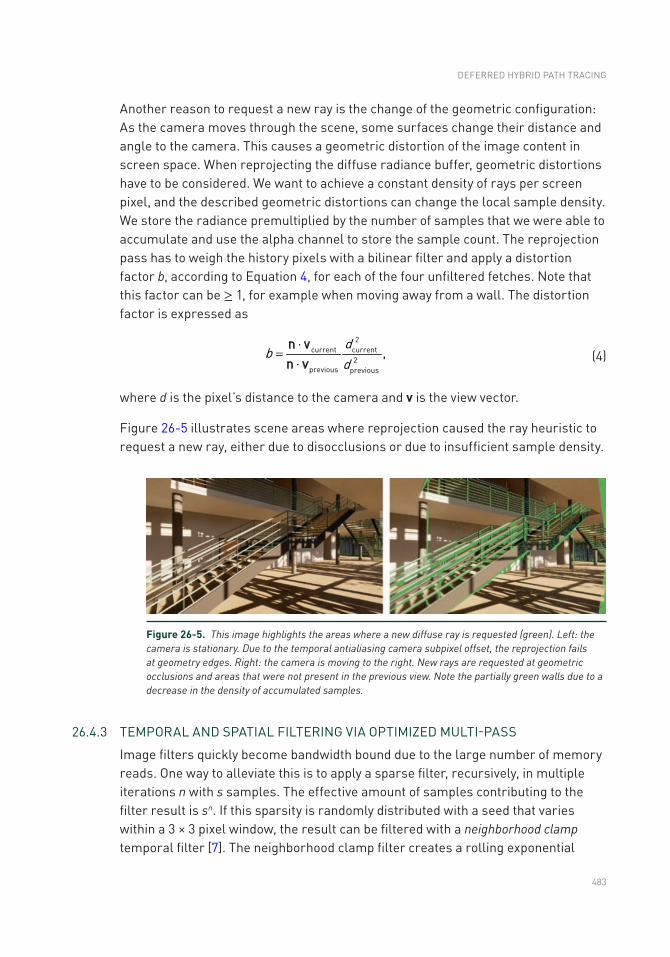
483
Another reason to request a new ray is the change of the geometric configuration: As the camera moves through the scene, some surfaces change their distance and angle to the camera. This causes a geometric distortion of the image content in screen space. When reprojecting the diffuse radiance buffer, geometric distortions have to be considered. We want to achieve a constant density of rays per screen pixel, and the described geometric distortions can change the local sample density. We store the radiance premultiplied by the number of samples that we were able to accumulate and use the alpha channel to store the sample count. The reprojection pass has to weigh the history pixels with a bilinear filter and apply a distortion factor b, according to Equation 4, for each of the four unfiltered fetches. Note that this factor can be ≥ 1, for example when moving away from a wall. The distortion factor is expressed as
d
bd
2current current
2previous previous
·,
·=
n vn v (4)
where d is the pixel’s distance to the camera and v is the view vector.
Figure 26-5 illustrates scene areas where reprojection caused the ray heuristic to request a new ray, either due to disocclusions or due to insufficient sample density.
26.4.3 TEMPORAL AND SPATIAL FILTERING VIA OPTIMIZED MULTI-PASS
Image filters quickly become bandwidth bound due to the large number of memory reads. One way to alleviate this is to apply a sparse filter, recursively, in multiple iterations n with s samples. The effective amount of samples contributing to the filter result is sn. If this sparsity is randomly distributed with a seed that varies within a 3 × 3 pixel window, the result can be filtered with a neighborhood clamp temporal filter [7]. The neighborhood clamp filter creates a rolling exponential
Figure 26-5. This image highlights the areas where a new diffuse ray is requested (green). Left: the camera is stationary. Due to the temporal antialiasing camera subpixel offset, the reprojection fails at geometry edges. Right: the camera is moving to the right. New rays are requested at geometric occlusions and areas that were not present in the previous view. Note the partially green walls due to a decrease in the density of accumulated samples.
DEFERRED HYBRID PATH TRACING
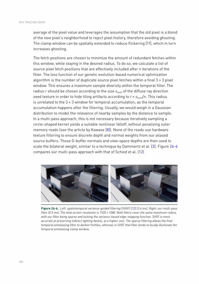
484
average of the pixel value and leverages the assumption that the old pixel is a blend of the new pixel’s neighborhood to reject pixel history, therefore avoiding ghosting. The clamp window can be spatially extended to reduce flickering [11], which in turn increases ghosting.
The fetch positions are chosen to minimize the amount of redundant fetches within this window, while staying in the desired radius. To do so, we calculate a list of source pixel fetch positions that are effectively included after n iterations of the filter. The loss function of our genetic evolution-based numerical optimization algorithm is the number of duplicate source pixel fetches within a final 3 × 3 pixel window. This ensures a maximum sample diversity within the temporal filter. The radius r should be chosen according to the size sseed of the diffuse ray direction seed texture in order to hide tiling artifacts according to r = sseed/n. This radius is unrelated to the 3 × 3 window for temporal accumulation, as the temporal accumulation happens after the filtering. Usually, we would weigh in a Gaussian distribution to model the relevance of nearby samples by the distance to sample. In a multi-pass approach, this is not necessary because iteratively sampling a circle-shaped kernel yields a suitable nonlinear falloff, without penalizing outer memory reads (see the article by Kawase [8]). None of the reads use hardware texture filtering to ensure discrete depth and normal weights from our aliased source buffers. Those G-buffer normals and view-space depths are then used to scale the bilateral weight, similar to a technique by Dammertz et al. [3]. Figure 26-6 compares our multi-pass approach with that of Schied et al. [12]
Figure 26-6. Left: spatiotemporal variance-guided filtering (SVGF) [12] (2.6 ms). Right: our multi-pass filter (0.5 ms). The total screen resolution is 1920 × 1080. Both filters cover the same maximum radius, with our filter being sparse and lacking the variance-based edge-stopping function. SVGF is more accurate at preserving indirect lighting details, at a higher cost. The sparse filtering allows the final temporal antialiasing filter to darken fireflies, whereas in SVGF that filter tends to locally illuminate the temporal antialiasing clamp window.
RAY TRACING GEMS
485
26.5 SPECULAR LIGHT TRANSPORT
Unlike diffuse filtering, specular filtering is prone to visually overblur details in reflections. We have to carefully pick and weigh the samples that we merge to create an estimate of the specular lobe. Inspired by Stachowiak [13], we trace our specular rays in half resolution and resolve to full resolution afterward using a ratio estimator. The introduced bias is acceptable, and the estimator is able to preserve normal map details and roughness variations. The major challenge remains in reducing noise in high-variance scenarios, such as rough metallic surfaces, while adding as little bias as possible. During sampling, we only importance-sample our microfacet’s distribution term. The Fresnel and geometry terms are approximated by a lookup table [6].
26.5.1 TEMPORAL ACCUMULATION
Similar to the diffuse pass, we try to find the pixel’s history by reprojecting its position into our previous specular buffer. This is done by using the virtual ray length correction techniques of Stachowiak [13] and Aizenshtein [1]. To avoid artifacts due to hardware bilinear filtering, we have to weigh the four bilinear samples individually and keep track of the total weight. In a case where the reprojection fails completely, like a disocclusion, we can only use the newly upsampled result. We use a 3 × 3 Gaussian blurred version of the upsampled buffer with a nonlinearity, like the perceptual quantizer electro- optical transfer function (used as a gamma curve in high dynamic range video signal processing), to hide fireflies.
The variance-based neighborhood clamp of temporal filtering allows us to discard incorrect reprojections. However, if the targeted radiance is occasionally not part of the local YCoCg bounding box, then flickering occurs. This can be countered by biasing the specular lobe [13], applying a variance-based post filter after temporal accumulation [14], enlarging the spatial size of the neighborhood, or simply darkening the bright pixels that introduce the bias. We observe that the flickering is mostly caused by a temporally unstable maximum luminance component. Therefore, we chose to temporally smooth the maximum luminance of the resulting color clamp. This only requires storing one additional value and causes few side effects.
DEFERRED HYBRID PATH TRACING

486
26.5.2 REUSE OF DIFFUSE LOBE
The specular pass is performed after the diffuse pass. We reuse the filtered diffuse result in our specular pass for two reasons:
> Low-variance fallback for high-roughness, dielectric specular lobes: Using the diffuse lobe as an approximation for the specular lobe is inaccurate. However, it is visually plausible since the lobe energy resides in a similar range. This saves performance on rough surfaces with moderate visual impact. For metals, we cannot rely on this simplification because the specular component is too visible.
> Ambient lighting amount for the geometry in the reflection: In cases where we do not want to trace further and gather the incoming lighting at the hit point, we need to assume an ambient lighting factor. The reflective surface’s diffuse lighting proved to be a good approximation with little cost.
26.5.3 PATH TRACED INDIRECT LIGHTING
Adding path traced indirect lighting is required for mirror-like surfaces. It is costly due to its incoherent memory reads and suffers from high variance. Liu [10] proposes filtering the indirect diffuse component along with the indirect diffuse component of the mirrored surfaces. To properly decouple the filtered lighting from albedo and direct light, we would need to store and fetch multiple additional buffers for our reflections. Instead, we chose to filter across the dimensions of the random seed texture (5 × 5 in our case) during the resolve pass, combined with a tone-mapped average to reduce fireflies. The filter is bilateral and takes the reflection ray length and G-buffer normal into account to preserve geometry silhouettes in reflections and normal map details. Both the special filtering and the indirect diffuse filtering is only applied for low-roughness metal surfaces, which makes the extra work affordable. A faster variant, without tracing additional rays, consists of the ambient factor combined with a screen-space ambient occlusion factor based on the ray lengths, which can be interpreted as virtual screen depth.
26.5.4 LOBE FOOTPRINT ESTIMATION
Similar to Liu’s work [10], we scale the number of filtering fetches according to the screen-space size of the projected reflection lobe footprint. This can be done by calculating the dimensions of a two-dimensional scale matrix.
Since most surfaces are not planar, we also need to estimate the local curvature and distort the footprint accordingly. This is done by computing the local derivatives of the G-buffer normal. The neighbors are chosen according to the eigenvectors of
RAY TRACING GEMS
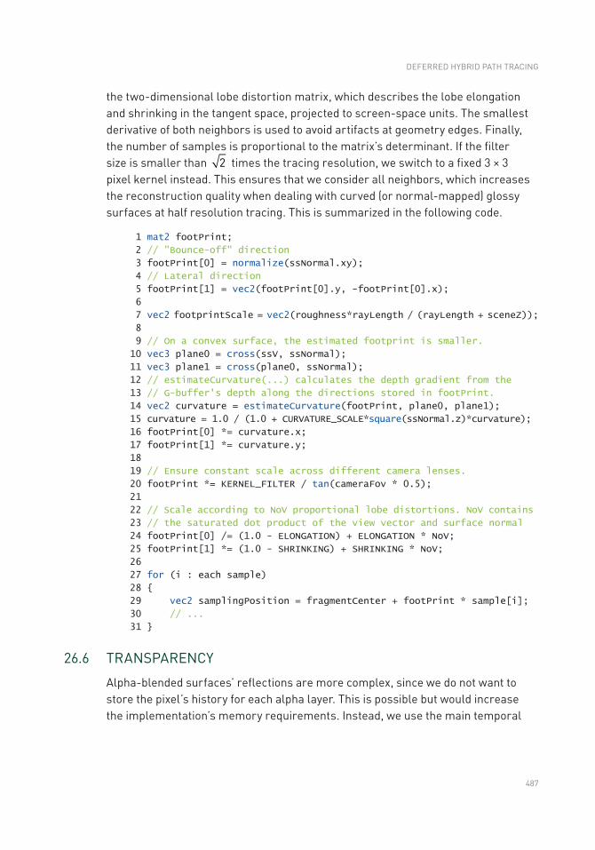
487
the two- dimensional lobe distortion matrix, which describes the lobe elongation and shrinking in the tangent space, projected to screen-space units. The smallest derivative of both neighbors is used to avoid artifacts at geometry edges. Finally, the number of samples is proportional to the matrix’s determinant. If the filter size is smaller than 2 times the tracing resolution, we switch to a fixed 3 × 3 pixel kernel instead. This ensures that we consider all neighbors, which increases the reconstruction quality when dealing with curved (or normal-mapped) glossy surfaces at half resolution tracing. This is summarized in the following code.
1 mat2 footPrint;
2 // "Bounce-off" direction
3 footPrint[0] = normalize(ssNormal.xy);
4 // Lateral direction
5 footPrint[1] = vec2(footPrint[0].y, -footPrint[0].x);
6
7 vec2 footprintScale = vec2(roughness*rayLength / (rayLength + sceneZ));
8
9 // On a convex surface, the estimated footprint is smaller.
10 vec3 plane0 = cross(ssV, ssNormal);
11 vec3 plane1 = cross(plane0, ssNormal);
12 // estimateCurvature(...) calculates the depth gradient from the
13 // G-buffer's depth along the directions stored in footPrint.
14 vec2 curvature = estimateCurvature(footPrint, plane0, plane1);
15 curvature = 1.0 / (1.0 + CURVATURE_SCALE*square(ssNormal.z)*curvature);
16 footPrint[0] *= curvature.x;
17 footPrint[1] *= curvature.y;
18
19 // Ensure constant scale across different camera lenses.
20 footPrint *= KERNEL_FILTER / tan(cameraFov * 0.5);
21
22 // Scale according to NoV proportional lobe distortions. NoV contains
23 // the saturated dot product of the view vector and surface normal
24 footPrint[0] /= (1.0 - ELONGATION) + ELONGATION * NoV;
25 footPrint[1] *= (1.0 - SHRINKING) + SHRINKING * NoV;
26
27 for (i : each sample)
28
29 vec2 samplingPosition = fragmentCenter + footPrint * sample[i];
30 // ...
31
26.6 TRANSPARENCY
Alpha-blended surfaces’ reflections are more complex, since we do not want to store the pixel’s history for each alpha layer. This is possible but would increase the implementation’s memory requirements. Instead, we use the main temporal
DEFERRED HYBRID PATH TRACING
488
antialiasing filter to take care of stochastic noise. This is acceptable because we assume that most alpha-blended surfaces (like glass) have a low roughness and therefore do not suffer from much variance during importance sampling of the specular distribution. Our order-independent transparency approach sorts the alpha pixels into layers before shading them, which allows us to employ different quality settings for each layer. We trace all layers in half resolution, just as for our specular component on opaque geometry. In contrast to the specular pass, we lack a G-buffer, which is why we cannot use the identical upscale algorithm. Instead, we implement a spatiotemporal shuffle by using blue noise–based offsets per pixel in the full resolution pass. This can be seen as a blur filter with only one fetch. Combined with the temporal antialiasing filter, this can be used to trade undersampling artifacts with noise.
26.7 PERFORMANCE
The performance results were measured using NVIDIA Titan V hardware at a resolution of 1920 × 1080. The current implementation still uses custom shaders for traversal, instead of DirectX Raytracing, for example. The scene contains 15 million polygons and represents an average architectural scene, as shown in Figure 26-7. The total frame time during these measurements was continuously below 9 ms.
RAY TRACING GEMS
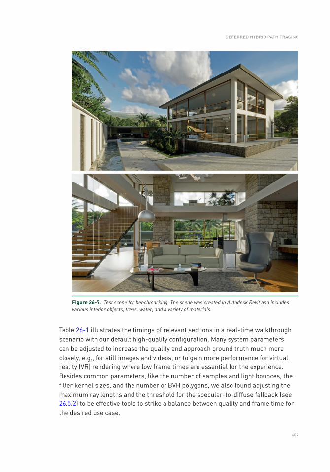
489
Figure 26-7. Test scene for benchmarking. The scene was created in Autodesk Revit and includes various interior objects, trees, water, and a variety of materials.
Table 26-1 illustrates the timings of relevant sections in a real-time walkthrough scenario with our default high-quality configuration. Many system parameters can be adjusted to increase the quality and approach ground truth much more closely, e.g., for still images and videos, or to gain more performance for virtual reality (VR) rendering where low frame times are essential for the experience. Besides common parameters, like the number of samples and light bounces, the filter kernel sizes, and the number of BVH polygons, we also found adjusting the maximum ray lengths and the threshold for the specular-to-diffuse fallback (see 26.5.2) to be effective tools to strike a balance between quality and frame time for the desired use case.
DEFERRED HYBRID PATH TRACING
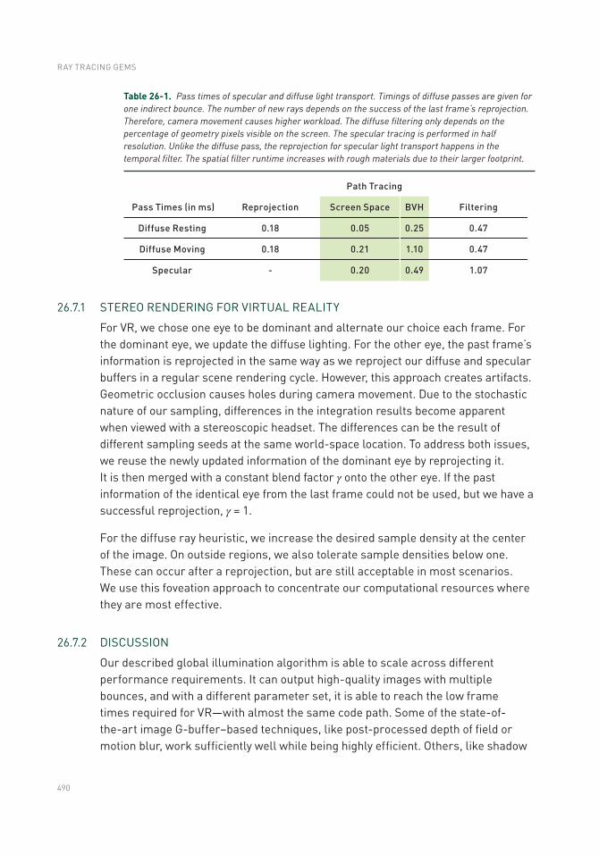
490
26.7.1 STEREO RENDERING FOR VIRTUAL REALITY
For VR, we chose one eye to be dominant and alternate our choice each frame. For the dominant eye, we update the diffuse lighting. For the other eye, the past frame’s information is reprojected in the same way as we reproject our diffuse and specular buffers in a regular scene rendering cycle. However, this approach creates artifacts. Geometric occlusion causes holes during camera movement. Due to the stochastic nature of our sampling, differences in the integration results become apparent when viewed with a stereoscopic headset. The differences can be the result of different sampling seeds at the same world-space location. To address both issues, we reuse the newly updated information of the dominant eye by reprojecting it. It is then merged with a constant blend factor γ onto the other eye. If the past information of the identical eye from the last frame could not be used, but we have a successful reprojection, γ = 1.
For the diffuse ray heuristic, we increase the desired sample density at the center of the image. On outside regions, we also tolerate sample densities below one. These can occur after a reprojection, but are still acceptable in most scenarios. We use this foveation approach to concentrate our computational resources where they are most effective.
26.7.2 DISCUSSION
Our described global illumination algorithm is able to scale across different performance requirements. It can output high-quality images with multiple bounces, and with a different parameter set, it is able to reach the low frame times required for VR—with almost the same code path. Some of the state-of-the-art image G-buffer–based techniques, like post-processed depth of field or motion blur, work sufficiently well while being highly efficient. Others, like shadow
Table 26-1. Pass times of specular and diffuse light transport. Timings of diffuse passes are given for one indirect bounce. The number of new rays depends on the success of the last frame’s reprojection. Therefore, camera movement causes higher workload. The diffuse filtering only depends on the percentage of geometry pixels visible on the screen. The specular tracing is performed in half resolution. Unlike the diffuse pass, the reprojection for specular light transport happens in the temporal filter. The spatial filter runtime increases with rough materials due to their larger footprint.
RAY TRACING GEMS
491
mapping, can be improved by ray tracing. Replacing a high number of shadow-mapped lights by ray tracing remains a performance challenge, yet it already promises high-quality results [5].
We also see room for improvement in the scalability of ray traced reflections on multiple alpha-blended layers. This is related to the calculation of subsurface scattering phenomena that are currently approximated by lighting in a volume texture in our case. For diffuse and specular integration, we would like to make specular ray tracing benefit from a ray heuristic, instead of equally sampling all screen regions each frame.
ACKNOWLEDGMENTS
We thank Tomasz Stachowiak and the editors for their valuable input, corrections, and suggestions that greatly improved this chapter.
REFERENCES
[1] Aizenshtein, M., and McMullen, M. New Techniques for Accurate Real-Time Reflections. Advanced Graphics Techniques Tutorial, SIGGRAPH Courses, 2018.
[2] Cranley, R., and Patterson, T. N. L. Randomization of Number Theoretic Methods for Multiple Integration. SIAM Journal on Numerical Analysis 13, 6 (1976), 904–914.
[3] Dammertz, H., Sewtz, D., Hanika, J., and Lensch, H. P. A. Edge-Avoiding À-Trous Wavelet Transform for Fast Global Illumination Filtering. In Proceedings of High- Performance Graphics (2010), pp. 67–75.
[4] Halton, J. H. Algorithm 247: Radical-Inverse Quasi-Random Point Sequence. Communications of the ACM 7, 12 (1964), 701–702.
[5] Heitz, E., Hill, S., and McGuire, M. Combining Analytic Direct Illumination and Stochastic Shadows. In Symposium on Interactive 3D Graphics and Games (2018), pp. 2:1–2:11.
[6] Karis, B. Real Shading in Unreal Engine 4. Physically Based Shading in Theory and Practice, SIGGRAPH Courses, August 2013.
[7] Karis, B. High-Quality Temporal Supersampling. Advances in Real-Time Rendering in Games, SIGGRAPH Courses, 2014.
[8] Kawase, M. Frame Buffer Postprocessing Effects in DOUBLE-S.T.E.A.L (Wreckless). Game Developers Conference, 2003.
[9] Kensler, A. Correlated Multi-Jittered Sampling. Pixar Technical Memo 13-01, 2013.
[10] Liu, E. Real-Time Ray Tracing: Low Sample Count Ray Tracing with NVIDIA’s Ray Tracing Denoisers. Real-Time Ray Tracing, SIGGRAPH NVIDIA Exhibitor Session, 2018.
DEFERRED HYBRID PATH TRACING

492
[11] Salvi, M. High Quality Temporal Supersampling. Real-Time Rendering Advances from NVIDIA Research, Game Developers Conference, 2016.
[12] Schied, C., Kaplanyan, A., Wyman, C., Patney, A., Chaitanya, C. R. A., Burgess, J., Liu, S., Dachsbacher, C., Lefohn, A. E., and Salvi, M. Spatiotemporal Variance- Guided Filtering: Real-Time Reconstruction for Path-Traced Global Illumination. In Proceedings of High-Performance Graphics (2017), pp. 2:1–2:12.
[13] Stachowiak, T. Stochastic Screen-Space Reflections. Advances in Real-Time Rendering in Games, SIGGRAPH Courses, 2015.
[14] Stachowiak, T. Towards Effortless Photorealism through Real-Time Raytracing. Computer Entertainment Developers Conferences, 2018.
Open Access This chapter is licensed under the terms of the Creative Commons Attribution-NonCommercial-NoDerivatives 4.0 International License (http://creativecommons.org/licenses/by-nc-nd/4.0/), which permits any noncommercial use, sharing, distribution and
reproduction in any medium or format, as long as you give appropriate credit to the original author(s) and the source, provide a link to the Creative Commons license and indicate if you modified the licensed material. You do not have permission under this license to share adapted material derived from this chapter or parts of it.
The images or other third party material in this chapter are included in the chapter's Creative Commons license, unless indicated otherwise in a credit line to the material. If material is not included in the chapter's Creative Commons license and your intended use is not permitted by statutory regulation or exceeds the permitted use, you will need to obtain permission directly from the copyright holder.
RAY TRACING GEMS
493© NVIDIA 2019 E. Haines, T. Akenine-Möller (eds.), Ray Tracing Gems, https://doi.org/10.1007/978-1-4842-4427-2_27
CHAPTER 27
Interactive Ray Tracing Techniques for High- Fidelity Scientific VisualizationJohn E. StoneBeckman Institute for Advanced Science and Technology,University of Illinois at Urbana-Champaign
ABSTRACT
This chapter describes rendering techniques and implementation considerations when using ray tracing for interactive scientific and technical visualization. Ray tracing offers a convenient framework for building high-fidelity rendering engines that can directly generate publication-quality images for scientific manuscripts while also providing high interactivity in a what-you-see-is-what-you-get rendering experience. The combination of interactivity with sophisticated rendering enables scientists who are typically not experts in computer graphics or rendering technologies to be able to immediately apply advanced rendering features in their daily work. This chapter summarizes techniques and practical approaches learned from applying ray tracing techniques to scientific visualization, and molecular visualization in particular.
27.1 INTRODUCTION
Scientific and technical visualizations are used to illustrate complex data, concepts, and physical phenomena to aid in the development of hypotheses, discover design problems, facilitate collaboration, and inform decision making. The scenes that arise in such visualizations incorporate graphical representations of the details of key structures and mechanisms and their relationships, or the dynamics of complex processes under study. High-quality ray tracing techniques have been of great use in the creation of visualizations that elucidate complex scenes. Interactivity is a powerful aid to the effectiveness of scientific visualization because it allows the visualization user to rapidly explore and manipulate data, models, and graphical representations to obtain insights and to help confirm or deny hypotheses.
Some of the challenges that arise in creating easy-to-understand visualizations involve compromises between what is shown in complete detail, what is shown just to provide important visual context, and what has to be eliminated (often sacrificed) for the sake of clarity of the visual communication. Advanced rendering techniques offer a variety of solutions to these kinds of problems. The relative ease with which
494
ray tracing algorithms can incorporate advanced lighting and shading models, and support a diverse range of geometric primitives and data types, make it a powerful tool for interactive rendering of geometrically complex scenes that arise in scientific and technical visualizations [2, 7, 17, 20, 24, 25].
Although ray tracing has been used for production of such visualizations in an offline or batch mode basis for decades, it has only recently reached performance levels that have made it strongly competitive with incumbent methods based on rasterization, wherein interactivity is a key requirement. The development of high-performance hardware-optimized ray tracing frameworks, and most recently ray tracing–specific hardware acceleration technologies available in commodity GPUs, has created the necessary conditions for broad use of interactive ray tracing for scientific visualization [13, 25, 26]. ParaView, VisIt, Visual Molecular Dynamics (VMD), and Visualization ToolKit (VTK)—several of the most widely used scientific visualization tools in high- performance computing—have each incorporated interactive ray tracing capabilities in the past few years. The performance gains provided by recent and upcoming ray tracing–specific hardware acceleration will hereafter create many new opportunities for interactive ray tracing to be applied in routine scientific and technical visualizations.
The remaining discussions and code samples provided in this chapter are intended to document some of the considerations, practical techniques, and elements of future outlook gained from the experience of developing and integrating three different interactive ray tracing engines within VMD, a widely used molecular visualization tool [5, 17, 19, 20, 21].
27.2 CHALLENGES ASSOCIATED WITH RAY TRACING LARGE SCENES
One of the recurring challenges that frequently arises in scientific visualization is the necessity to render scenes that reach the limits of available physical memory. Visualization approaches based on rasterization benefit from its streaming nature and typically low memory requirements. Conversely, ray tracing methods require the entire scene description to be retained in memory or made available to the ray tracing engine on demand. This is one of the key trade-offs of ray tracing methods in exchange for their flexibility, elegance, and adaptability to a wide range of rendering and visualization problems.
At the time of writing, tremendous gains in ray tracing performance have been achieved on GPUs through dedicated hardware that accelerates both bounding volume hierarchy (BVH) traversal and ray/triangle intersection tests. This advance has increased ray tracing performance to such a degree that, for scientific
RAY TRACING GEMS
495
visualizations employing relatively low-cost shading, memory bandwidth is now and will likely remain one of the critical factors limiting peak ray tracing performance for the foreseeable future. Considering these issues together, it is clear that the long-term successful application of ray tracing in challenging scientific visualization scenarios will depend on the development and application of techniques that make efficient use of both memory capacity and memory bandwidth.
27.2.1 USING THE RIGHT GEOMETRIC PRIMITIVE FOR THE JOB
Some of the best opportunities for savings in memory capacity and memory bandwidth relate to the choice of geometric primitives used to construct visualizations. As an example, the memory footprint for a sphere position and radius is just 4 floating-point values, whereas an individual triangle with per-vertex normals and no shared vertices requires 18 values. When representing a triangle mesh, shared vertices can be listed explicitly with vertex indices (three vertex array indices per triangle), or better yet, when feasible, they can be implied by triangle strip vertex index ordering (three indices for the first triangle, and only one index for each subsequent triangle). The memory cost of surface normals can be reduced by quantizing or compressing them significantly, further reducing the memory cost per vertex and per triangle. Ultimately, while these and related techniques can significantly reduce the memory cost for triangle meshes, direct ray tracing of spheres, cylinders, or cones rather than small triangle meshes will likely always use less memory and, more importantly in the long term, consume less memory bandwidth. While it is clear that for some domains, such as molecular visualization, large memory efficiency gains can be had through the use of a handful of bespoke geometric primitive implementations, in other scientific domains it is less clear, and the alternative geometric primitives available for consideration might involve numerical precision or convergence challenges in ray/primitive intersection test implementation, or performance attributes or anomalies that make them difficult to use effectively in all cases.
27.2.2 ELIMINATION OF REDUNDANCY, COMPRESSION, AND QUANTIZATION
Once the best choice of geometric primitives has been made, the remaining low-cost opportunities for reducing memory capacity and bandwidth requirements tend to be methods that eliminate high-level redundancies within large batches of geometric primitives. For example, particle advection streamlines used for visualization of fluid flow, magnetic fields, or electrostatic potential fields may contain millions of segments. Why store a radius per cylinder or per sphere when drawing tubular streamlines if all constituent segments have the same radius?
INTERACTIVE RAY TRACING TECHNIQUES FOR HIGH- FIDELITY SCIENTIFIC VISUALIZATION
496
In the same way that rasterization pipelines have supported a broad diversity of triangle mesh formats and per-vertex data, ray tracing engines stand to benefit from similar flexibility, but for a much broader range of potential geometric primitives. For example, a ray tracing engine used to render scenes containing large numbers of streamlines of various types might employ multiple specialized geometry batch types, with radii specified per cylinder and per sphere, and with constant radii for all constituent cylinders and spheres. Depending on the degree of programmability of the underlying ray tracing framework, it might be possible to cause cylinder and sphere primitives to share the same vertex data. Furthermore, it might be possible to implement a fully customized streamline rendering primitive that implements or emulates the effect of a swept sphere following a space curve defined by the original streamline vertices themselves or by computed control points fit to the original data [23]. The more programmability available in the ray tracing framework, the more easily an application can choose the geometric primitives and geometry batching approaches that are most beneficial for resolving the memory capacity and performance issues posed by large visualizations.
After high-level redundancies have been eliminated from the encoding and parameterization of large batches of geometry, the next areas to approach are techniques that eliminate more-localized data redundancies at the level of groups of neighboring or otherwise related geometric properties. Localized data size reductions can often be made through data compression approaches and reduced-precision quantized representations of geometric attributes, or combinations of the two. When quantization or other lossy compression techniques are used, acceptable error tolerances may depend on the details of the visualization problem at hand. Two representative examples of these techniques are compression of volumetric data, scalar fields, and tensors, e.g., as provided by the ZFP library [8, 9], and quantized representations of surface normals, as in octahedron normal vector encoding [4, 12]. See Listing 27-4 for an example implementation of normal packing and unpacking using octahedron normal encoding.
Listing 27-1. This code snippet lists the key functions required to implement normal packing and unpacking using octahedron normal vector encoding. The routines convert back and forth between normal vectors represented as three single-precision oating-point values and a single packed 32-bit unsigned integer encoding. Many performance optimizations and improvements are possible here, but these routines are easy to try out in your own ray tracing engine.
1 # include <optixu/optixu_math_namespace.h> // For make_xxx() functions
2
3 // Helper routines that implement the floating-point stages of
4 // octahedron normal vector encoding
RAY TRACING GEMS
497
5 static _ _host_ _ _ _device_ _ _ _inline_ _
6 float3 OctDecode(float2 projected)
7 float3 n;
8 n = make_float3(projected.x, projected.y,
9 1.0f - (fabsf(projected.x) + fabsf(projected.y)));
10 if (n.z < 0.0f)
11 float oldX = n.x;
12 n.x = copysignf(1.0f - fabsf(n.y), oldX);
13 n.y = copysignf(1.0f - fabsf(oldX), n.y);
14
15 return n;
16
17
18 static _ _host_ _ _ _device_ _ _ _inline_ _
19 float2 OctEncode(float3 n)
20 const float invL1Norm = 1.0f / (fabsf(n.x)+fabsf(n.y)+fabsf(n.z));
21 float2 projected;
22 if (n.z < 0.0f)
23 float2 tmp = make_float2(fabsf(n.y), fabsf(n.x));
24 projected = 1.0f - tmp * invL1Norm;
25 projected.x = copysignf(projected.x, n.x);
26 projected.y = copysignf(projected.y, n.y);
27 else
28 projected = make_float2(n.x, n.y) * invL1Norm;
29
30 return projected;
31
32
33 // Helper routines to quantize to or invert the quantization
34 // to and from packed unsigned integer representations
35 static _ _host_ _ _ _device_ _ _ _inline_ _
36 uint convfloat2uint32(float2 f2)
37 f2 = f2 * 0.5f + 0.5f;
38 uint packed;
39 packed = ((uint) (f2.x * 65535)) | ((uint) (f2.y * 65535) << 16);
40 return packed;
41
42
43 static _ _host_ _ _ _device_ _ _ _inline_ _
44 float2 convuint32float2(uint packed)
45 float2 f2;
46 f2.x = (float)((packed ) & 0x0000ffff) / 65535;
47 f2.y = (float)((packed >> 16) & 0x0000ffff) / 65535;
48 return f2 * 2.0f - 1.0f;
49
50
51 // The routines to be called when preparing geometry buffers prior
52 // to ray tracing and when decoding them on-the-fly during rendering
INTERACTIVE RAY TRACING TECHNIQUES FOR HIGH- FIDELITY SCIENTIFIC VISUALIZATION
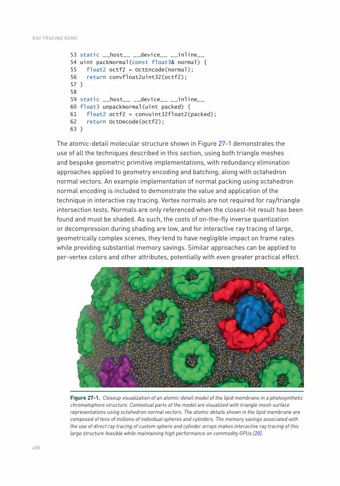
498
53 static _ _host_ _ _ _device_ _ _ _inline_ _
54 uint packNormal(const float3& normal)
55 float2 octf2 = OctEncode(normal);
56 return convfloat2uint32(octf2);
57
58
59 static _ _host_ _ _ _device_ _ _ _inline_ _
60 float3 unpackNormal(uint packed)
61 float2 octf2 = convuint32float2(packed);
62 return OctDecode(octf2);
63
The atomic-detail molecular structure shown in Figure 27-1 demonstrates the use of all the techniques described in this section, using both triangle meshes and bespoke geometric primitive implementations, with redundancy elimination approaches applied to geometry encoding and batching, along with octahedron normal vectors. An example implementation of normal packing using octahedron normal encoding is included to demonstrate the value and application of the technique in interactive ray tracing. Vertex normals are not required for ray/triangle intersection tests. Normals are only referenced when the closest-hit result has been found and must be shaded. As such, the costs of on-the-fly inverse quantization or decompression during shading are low, and for interactive ray tracing of large, geometrically complex scenes, they tend to have negligible impact on frame rates while providing substantial memory savings. Similar approaches can be applied to per-vertex colors and other attributes, potentially with even greater practical effect.
Figure 27-1. Closeup visualization of an atomic-detail model of the lipid membrane in a photosynthetic chromatophore structure. Contextual parts of the model are visualized with triangle mesh surface representations using octahedron normal vectors. The atomic details shown in the lipid membrane are composed of tens of millions of individual spheres and cylinders. The memory savings associated with the use of direct ray tracing of custom sphere and cylinder arrays makes interactive ray tracing of this large structure feasible while maintaining high performance on commodity GPUs [20].
RAY TRACING GEMS
499
27.2.3 CONSIDERATIONS FOR RAY TRACING ACCELERATION STRUCTURES
Beyond the direct memory cost associated with a given geometric primitive, it is important to consider the per-primitive memory costs associated with the BVH or other ray tracing acceleration structure that ultimately contains them. It can be surprising that, despite the use of data compression techniques in state-of-the-art ray tracing acceleration structures, the acceleration structures themselves can sometimes end up being as large or larger in size than the scene geometry they encode. Acceleration structures and their space-versus-time trade-offs are therefore an area of significant concern for applications of ray tracing to scientific visualizations. Since acceleration structure construction, storage, and traversal are all performance-critical aspects of ray tracing, they are frequently proprietary, highly hardware-optimized, and therefore often less flexible than one might prefer.
For visualization of static structures, large and highly optimized acceleration structures yield the best performance since construction and update costs are relatively unimportant. For interactive display of time series data such as simulation trajectories, time spent on geometry buffer updates and acceleration structure (re)builds becomes an important factor in interactivity. Time series animation is a much more complex case that can benefit significantly from increased concurrency, e.g., via multithreading techniques. To completely decouple geometry updates and acceleration structure (re)builds from ongoing interactive rendering and display, it is necessary to employ double- or multi-buffering of key ray tracing data structures. Multi-buffering of ray tracing data structures permits scene updates to occur concurrently and asynchronously with ongoing rendering.
The need for flexibility in ray tracing acceleration structure optimization is of particular interest for both large, static scenes and for dynamic time series visualizations. When visualizing large scientific scenes that have extremely high geometric complexity, often the memory required by the acceleration structure exceeds available capacity. In such cases it is usually preferable to build a moderately coarser acceleration structure that sacrifices some performance in favor of increased geometric capacity. The use of a coarser acceleration structure may also turn out to be a desirable trade-off for time series visualizations. Some existing ray tracing frameworks provide simple controls over acceleration structure construction heuristics and tunables for these purposes. This remains an area of active development where one can expect future ray tracing engines to make significant advances.
INTERACTIVE RAY TRACING TECHNIQUES FOR HIGH- FIDELITY SCIENTIFIC VISUALIZATION
500
27.3 VISUALIZATION METHODS
In this section, several simple but extremely useful ray tracing–compatible shading techniques are described, along with descriptions of their practical use and implementation. Scientists and technicians who use visualization tools have tremendous domain expertise, but they often have only moderate familiarity with optics, lighting, shading, and computer graphics techniques in general. A key component of the techniques described here is that they are easily used by nonexpert visualization practitioners, particularly when implemented in a fully interactive ray tracing engine with progressive refinement and other niceties. A panoply of excellent shading techniques are available for scientific visualization applications based on rasterization. However, many of these depend on rasterization-specific techniques or API features, and they may not be compatible with the range of lighting and shading techniques commonly used in interactive ray tracing visualization engines. The techniques described next have low performance costs, can be combined with other ray tracing features, and, most importantly, have seen ongoing use in the creation of effective visualizations.
The ray tracing methods described here provide several useful scientific visualization tools for ambient occlusion lighting, non-photorealistic transparent surfaces, edge outlining of opaque surfaces, and clipping planes and spheres, each of which can contribute to improving the clarity and interpretation of resulting visualizations.
27.3.1 AMBIENT OCCLUSION LIGHTING IN SCIENTIFIC VISUALIZATION
A key value of ambient occlusion (AO) lighting for scientific and technical visualization is its tremendous time savings, particularly when paired with complex scenes and other high-fidelity ray tracing techniques. AO can be useful for interactive viewing of complex models, but especially for time series data such as simulation trajectories, when it is impractical for a user to continually adjust manually placed lights to achieve a desirable lighting outcome [19, 22]. The “ambient” aspect of AO lighting is what makes it such a convenient tool for nonexpert users. With interactive use of AO and progressive ray tracing, users need not become experts at lighting design and can instead achieve a “good” lighting arrangement by adjusting one or two key ambient occlusion lighting parameters, typically in combination with one or two manually positioned directional or point light sources. This is particularly true in domains such as molecular visualization, where the visualization lighting design is solely for elucidating details of molecular structure and is not an attempt to replicate a photorealistic scene of some sort. One way in which the application of AO can be made easy for beginners is to provide independent light scaling factors for both
RAY TRACING GEMS
501
AO (“ambient”) and manually placed (“direct”) light sources. By providing separate easy-to-use global intensity scaling factors for ambient and direct lighting, beginners find it easier to balance their lighting design and avoid both over-lit and under-lit conditions that can otherwise easily occur in geometrically complex scenes that contain pockets, pores/tunnels, or cavities that each pose lighting challenges.
27.3.1.1 AO WITH LIMITED OCCLUSION DISTANCE
A problem with AO that often arises when exploring scenes with densely packed geometry is that there are few paths for the “ambient” light to get deep within a complex structure, such as within a virus capsid or a cell membrane. A simple but effective solution to this problem is to compute AO lighting with a maximum occlusion distance, beyond which ambient occlusions are ignored. Using this technique, one can choose a maximum occlusion distance that comfortably fits within the confined viewing spaces of interest, maintaining the key benefits of AO for visualization purposes, as shown in Figure 27-2. While a camera-centered point light could be used to light dark interiors of largely or fully enclosed structures, it would result in an undesirable flat-looking surface. This too could be resolved by careful manual or offset placement of multiple point lights or area lights, but such tasks are ultimately undesirable distractions that take away from unrestricted interactive exploration of complex models or simulation results. The use of AO with a limited occlusion distance avoids these undesirable issues while maintaining unrestricted interactive scene navigation. A further, perhaps unanticipated, benefit of this type of approach is that the maximum AO occlusion distance can also be used to shadow only pores, pockets, and cavities of a particular maximum diameter range, converting AO lighting into a tool capable of highlighting particular geometric features with a mild degree of selectivity. This technique can be refined further by incorporating user-specified AO falloff attenuation coefficients, if desired. See Listing 27-2 for a simple example implementation.
INTERACTIVE RAY TRACING TECHNIQUES FOR HIGH- FIDELITY SCIENTIFIC VISUALIZATION
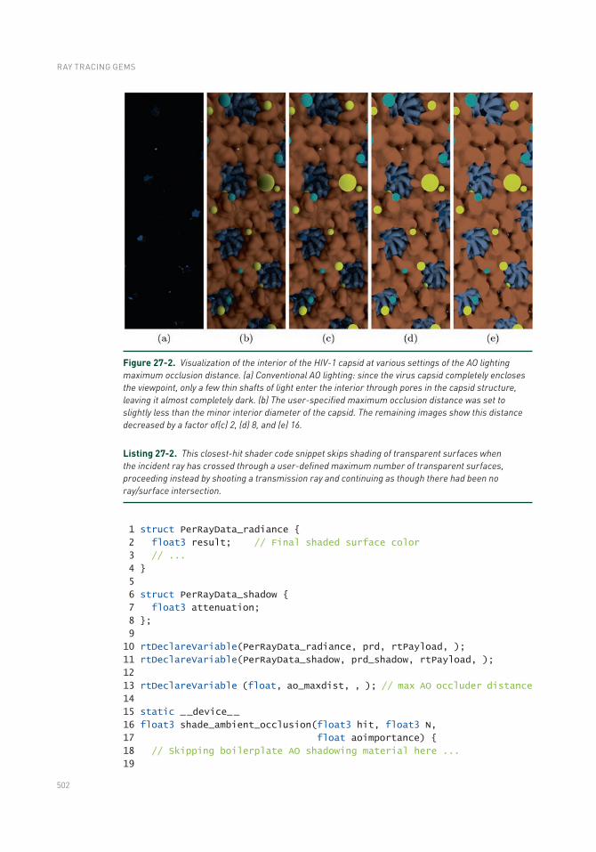
502
Listing 27-2. This closest-hit shader code snippet skips shading of transparent surfaces when the incident ray has crossed through a user- defined maximum number of transparent surfaces, proceeding instead by shooting a transmission ray and continuing as though there had been no ray/surface intersection.
1 struct PerRayData_radiance
2 float3 result; // Final shaded surface color
3 // ...
4
5
6 struct PerRayData_shadow
7 float3 attenuation;
8 ;
9
10 rtDeclareVariable(PerRayData_radiance, prd, rtPayload, );
11 rtDeclareVariable(PerRayData_shadow, prd_shadow, rtPayload, );
12
13 rtDeclareVariable (float, ao_maxdist, , ); // max AO occluder distance
14
15 static _ _device_ _
16 float3 shade_ambient_occlusion(float3 hit, float3 N,
17 float aoimportance)
18 // Skipping boilerplate AO shadowing material here ...
19
Figure 27-2. Visualization of the interior of the HIV-1 capsid at various settings of the AO lighting maximum occlusion distance. (a) Conventional AO lighting: since the virus capsid completely encloses the viewpoint, only a few thin shafts of light enter the interior through pores in the capsid structure, leaving it almost completely dark. (b) The user-specified maximum occlusion distance was set to slightly less than the minor interior diameter of the capsid. The remaining images show this distance decreased by a factor of(c) 2, (d) 8, and (e) 16.
RAY TRACING GEMS
503
20 for (int s=0; s<ao_samples; s++)
21 Ray aoray;
22 // Skipping boilerplate AO shadowing material here ...
23 aoray = make_Ray (hit, dir, shadow_ray_type,
24 scene_epsilon, ao_maxdist);
25
26 shadow_prd.attenuation = make_float3(1.0f);
27 rtTrace(root_shadower, ambray, shadow_prd);
28 inten += ndotambl * shadow_prd.attenuation;
29
30
31 return inten * lightscale;
32
33
34 RT_PROGRAM void closest_hit_shader( ... )
35 // Skipping boilerplate closest-hit shader material here ...
36
37 // Add ambient occlusion diffuse lighting, if enabled.
38 if (AO_ON && ao_samples > 0)
39 result *= ao_direct;
40 result += ao_ambient * col * p_Kd *
41 shade_ambient_occlusion(hit_point, N, fogf * p_opacity);
42
43
44 // Continue with typical closest-hit shader contents ...
45
46 prd.result = result; // Pass the resulting color back up the tree.
47
27.3.1.2 REDUCING MONTE CARLO SAMPLING NOISE
Scientists who use visualization tools frequently need to generate quick “snapshot” renderings for routine use in team meetings and presentations. Being perpetually short of time, there is a tendency for users to prefer high-fidelity rendering approaches, but with the condition that rendering can be halted at any point, providing them with an image that is free of “grain” or “speckle,” albeit without having fully converged lighting or depth of field focal blur.
A particularly promising class of state-of-the-art techniques for real-time denoising employs carefully trained deep neural networks to eliminate grain and speckle noise in undersampled regions of images produced by Monte Carlo rendering [3, 6, 10, 15, 16]. The success of so-called artificially intelligent (AI) denoisers often depends on the availability of auxiliary image data buffers containing depth, surface normals, albedo, and other types of information that help the denoiser do a better job of identifying noise and undersampled image
INTERACTIVE RAY TRACING TECHNIQUES FOR HIGH- FIDELITY SCIENTIFIC VISUALIZATION
504
regions. The interactive-rate performance of AI denoisers also hinges upon the availability of hardware-accelerated AI inferencing, which enables the denoiser to outrun brute-force sampling, even on hardware platforms with dedicated ray tracing hardware acceleration. It appears likely that AI denoising will remain one of best and most broadly used approaches for denoising in sophisticated path tracing, and in ray tracing engines more generally, because the techniques can be tuned or trained specifically for particular renderers and scene content.
Besides sophisticated denoising techniques, one can also make potentially beneficial trade-offs between high-frequency noise content and the correlation of stochastic samples, e.g., resulting in visible AO shadow boundary edges in undersampled interactive renderings. In conventional ray tracing technique, ambient occlusion lighting and other Monte Carlo sampling implementations typically use completely uncorrelated pseudo-random or quasi-random number sequences to generate directions for AO lighting shadow feeler rays within the hemisphere normal to the surface being shaded. With an uncorrelated sampling approach, when a sufficient number of AO lighting samples have been taken, a smooth grain-free image results. However, early termination of an unconverged sampling process results in a grainy looking image. By purposefully correlating AO samples in all image pixels, e.g., by seeding AO random number generators or quasi-random sequence generators with the same seed, all pixels in the image will choose the same AO shadow feeler directions, and there will be no image grain from AO. This approach is particularly well suited for interactive ray tracing of geometrically complex scenes that would otherwise require a large number of samples to achieve grain-free images.
27.3.2 EDGE-ENHANCED TRANSPARENT SURFACES
A common problem that arises in molecular visualizations is the need to clearly display the boundaries of molecular complexes or their constituent substructures, while making it easy to see the details of their internal structures. Molecular scientists spend significant effort selecting what should be shown and how it should be displayed. Raster3D [11], Tachyon [18], and VMD [5, 20] employ special shaders that make it easy to see the interior of a structure by making viewer-directed surfaces entirely transparent, while leaving the boundary regions that are seen edge-on largely opaque. The surface shader instantly adapts to changes in viewing orientation, permitting the user to freely rotate the molecular complex while maintaining an unobscured view of interior details. This technique is demonstrated effectively in Figure 27-3, where it is applied to light- harvesting complexes and photosynthetic reaction centers, and in Figure 27-4, where it is applied to a solvent box and solvent/protein interface. See Listing 27-3 for the details of the shader implementation.
RAY TRACING GEMS
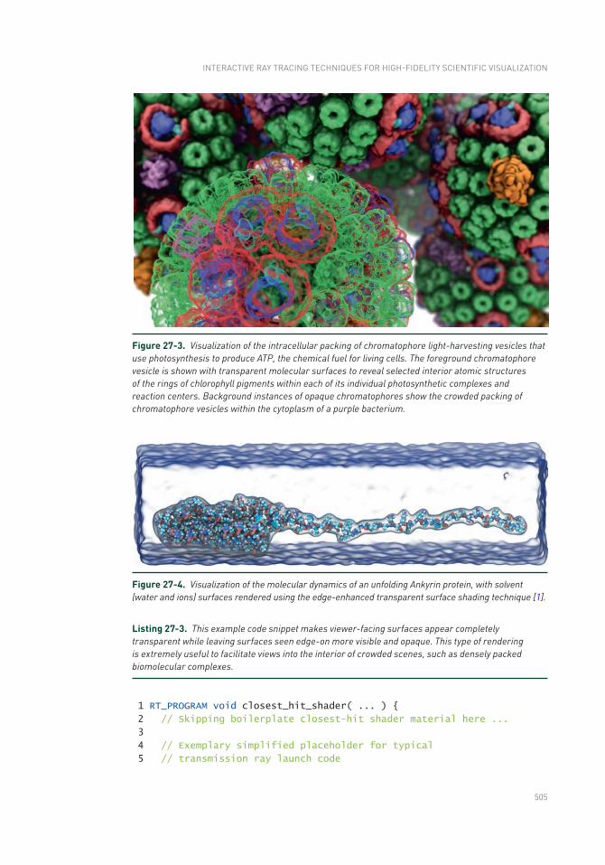
505
Listing 27-3. This example code snippet makes viewer-facing surfaces appear completely transparent while leaving surfaces seen edge-on more visible and opaque. This type of rendering is extremely useful to facilitate views into the interior of crowded scenes, such as densely packed biomolecular complexes.
1 RT_PROGRAM void closest_hit_shader( ... )
2 // Skipping boilerplate closest-hit shader material here ...
3
4 // Exemplary simplified placeholder for typical
5 // transmission ray launch code
Figure 27-3. Visualization of the intracellular packing of chromatophore light- harvesting vesicles that use photosynthesis to produce ATP, the chemical fuel for living cells. The foreground chromatophore vesicle is shown with transparent molecular surfaces to reveal selected interior atomic structures of the rings of chlorophyll pigments within each of its individual photosynthetic complexes and reaction centers. Background instances of opaque chromatophores show the crowded packing of chromatophore vesicles within the cytoplasm of a purple bacterium.
Figure 27-4. Visualization of the molecular dynamics of an unfolding Ankyrin protein, with solvent (water and ions) surfaces rendered using the edge-enhanced transparent surface shading technique [1].
INTERACTIVE RAY TRACING TECHNIQUES FOR HIGH- FIDELITY SCIENTIFIC VISUALIZATION
506
6 if (alpha < 0.999f)
7 // Emulate Tachyon/Raster3D's angle-dependent surface opacity
8 if (transmode)
9 alpha = 1.0f + cosf(3.1415926f * (1.0f-alpha) *
10 dot(N, ray.direction));
11 alpha = alpha*alpha * 0.25f;
12
13 result *= alpha; // Scale down lighting by any new transparency
14
15 // Skipping boilerplate code to prepare a new transmission ray ...
16 rtTrace(root_object, trans_ray, new_prd);
17
18 result += (1.0f - alpha) * new_prd.result;
19
20 // Continue with typical closest-hit shader contents ...
21
22 prd.result = result; // Pass the resulting color back up the tree.
23
27.3.3 PEELING AWAY EXCESS TRANSPARENT SURFACES
Many domains within scientific visualization produce scenes that incorporate significant amounts of partially transparent geometry, often to display surfaces within volumetric data of various types, e.g., electron density maps, medical images, tomograms from cryo-electron microscopy, or flow fields from computational fluid dynamics simulations. When rendering scenes containing complex or noisy volumetric data, transparent isosurfaces and contained geometry may become more difficult to interpret visually, and it is often helpful to create purposefully non-photorealistic renderings that “peel away” all but the first, or first few, layers of transparent surfaces so they do not create a distracting background behind features of particular interest. See Figure 27-5. Transparent surfaces can be peeled as described by making a small modification to a canonical closest-hit program: store an additional counter for transparent surface crossing as an extra per-ray data item. When primary rays are generated, the crossing counter is initially set to the maximum number of transparent surfaces to be shown. As the ray is traced through the scene, the per-ray transparent surface crossing counter is decremented on each transparent surface until it reaches zero. Once this happens, all subsequent intersections with transparent surfaces are ignored, i.e., they are not shaded and do not contribute to the final color, and transmission rays are generated to continue as if no intersection had occurred. See Listing 27-4 for an example implementation.
RAY TRACING GEMS
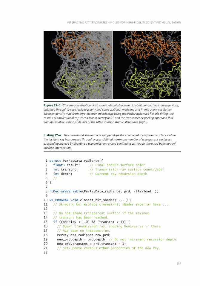
507
Listing 27-4. This closest-hit shader code snippet skips the shading of transparent surfaces when the incident ray has crossed through a user- defined maximum number of transparent surfaces, proceeding instead by shooting a transmission ray and continuing as though there had been no ray/surface intersection.
1 struct PerRayData_radiance
2 float3 result; // Final shaded surface color
3 int transcnt; // Transmission ray surface count/depth
4 int depth; // Current ray recursion depth
5 // ...
6
7
8 rtDeclareVariable(PerRayData_radiance, prd, rtPayload, );
9
10 RT_PROGRAM void closest_hit_shader( ... )
11 // Skipping boilerplate closest-hit shader material here ...
12
13 // Do not shade transparent surface if the maximum
14 // transcnt has been reached.
15 if ((opacity < 1.0) && (transcnt < 1))
16 // Spawn transmission ray; shading behaves as if there
17 // had been no intersection.
18 PerRayData_radiance new_prd;
19 new_prd.depth = prd.depth; // Do not increment recursion depth.
20 new_prd.transcnt = prd.transcnt - 1;
21 // Set/update various other properties of the new ray.
22
Figure 27-5. Closeup visualization of an atomic-detail structure of rabbit hemorrhagic disease virus, obtained through X-ray crystallography and computational modeling and fit into a low-resolution electron density map from cryo-electron microscopy using molecular dynamics flexible fitting: the results of conventional ray traced transparency (left), and the transparency peeling approach that eliminates obscuration of details of the fitted interior atomic structures (right).
INTERACTIVE RAY TRACING TECHNIQUES FOR HIGH- FIDELITY SCIENTIFIC VISUALIZATION
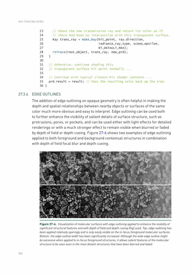
508
23 // Shoot the new transmission ray and return its color as if
24 // there had been no intersection with this transparent surface.
25 Ray trans_ray = make_Ray(hit_point, ray.direction,
26 radiance_ray_type, scene_epsilon,
27 RT_DEFAULT_MAX);
28 rtTrace(root_object, trans_ray, new_prd);
29
30
31 // Otherwise, continue shading this
32 // transparent surface hit point normally ...
33
34 // Continue with typical closest-hit shader contents ...
35 prd.result = result; // Pass the resulting color back up the tree.
36
27.3.4 EDGE OUTLINES
The addition of edge outlining on opaque geometry is often helpful in making the depth and spatial relationships between nearby objects or surfaces of the same color much more obvious and easy to interpret. Edge outlining can be used both to further enhance the visibility of salient details of surface structure, such as protrusions, pores, or pockets, and can be used either with light effects for detailed renderings or with a much stronger effect to remain visible when blurred or faded by depth of field or depth cueing. Figure 27-6 shows two examples of edge outlining applied to both foreground and background contextual structures in combination with depth of field focal blur and depth cueing.
Figure 27-6. Visualization of molecular surfaces with edge outlining applied to enhance the visibility of significant structural features and with depth of field and depth cueing (fog) used. Top: edge outlining has been applied relatively sparingly and is only easily visible on the in-focus foreground molecular surfaces. Bottom: the edge outline width has been significantly increased. Although the wide edge outline might be excessive when applied to in-focus foreground structures, it allows salient features of the molecular structure to be seen even in the most distant structures that have been blurred and faded.
RAY TRACING GEMS
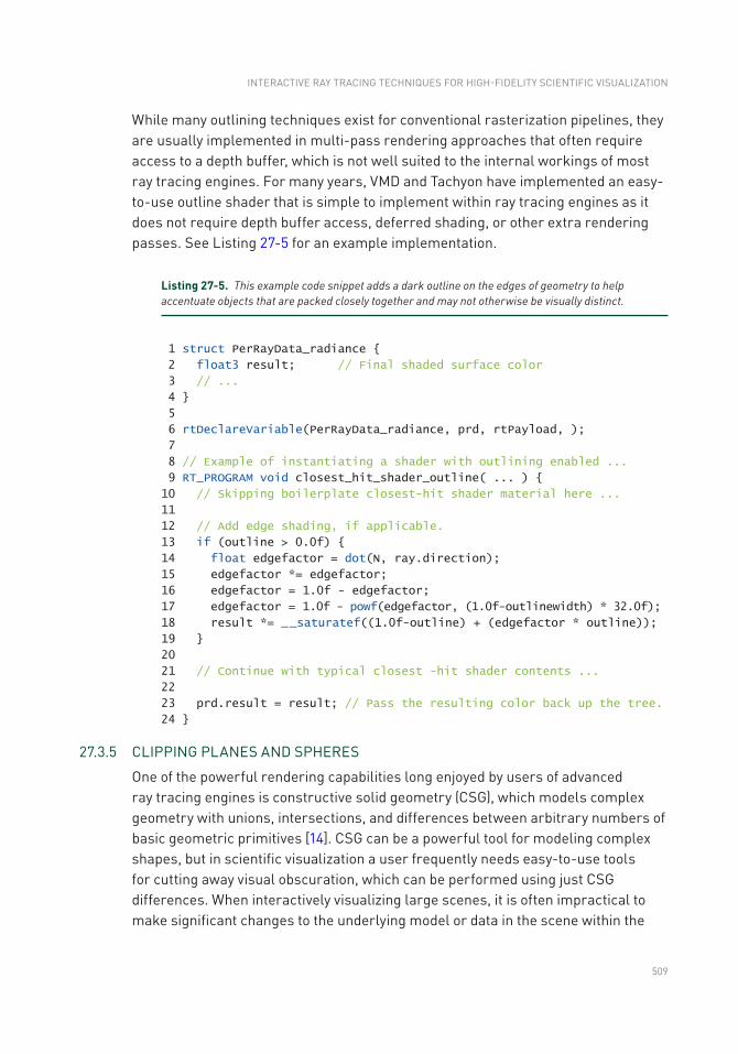
509
While many outlining techniques exist for conventional rasterization pipelines, they are usually implemented in multi-pass rendering approaches that often require access to a depth buffer, which is not well suited to the internal workings of most ray tracing engines. For many years, VMD and Tachyon have implemented an easy-to-use outline shader that is simple to implement within ray tracing engines as it does not require depth buffer access, deferred shading, or other extra rendering passes. See Listing 27-5 for an example implementation.
Listing 27-5. This example code snippet adds a dark outline on the edges of geometry to help accentuate objects that are packed closely together and may not otherwise be visually distinct.
1 struct PerRayData_radiance
2 float3 result; // Final shaded surface color
3 // ...
4
5
6 rtDeclareVariable(PerRayData_radiance, prd, rtPayload, );
7
8 // Example of instantiating a shader with outlining enabled ...
9 RT_PROGRAM void closest_hit_shader_outline( ... )
10 // Skipping boilerplate closest-hit shader material here ...
11
12 // Add edge shading, if applicable.
13 if (outline > 0.0f)
14 float edgefactor = dot(N, ray.direction);
15 edgefactor *= edgefactor;
16 edgefactor = 1.0f - edgefactor;
17 edgefactor = 1.0f - powf(edgefactor, (1.0f-outlinewidth) * 32.0f);
18 result *= _ _saturatef((1.0f-outline) + (edgefactor * outline));
19
20
21 // Continue with typical closest -hit shader contents ...
22
23 prd.result = result; // Pass the resulting color back up the tree.
24
27.3.5 CLIPPING PLANES AND SPHERES
One of the powerful rendering capabilities long enjoyed by users of advanced ray tracing engines is constructive solid geometry (CSG), which models complex geometry with unions, intersections, and differences between arbitrary numbers of basic geometric primitives [14]. CSG can be a powerful tool for modeling complex shapes, but in scientific visualization a user frequently needs easy-to-use tools for cutting away visual obscuration, which can be performed using just CSG differences. When interactively visualizing large scenes, it is often impractical to make significant changes to the underlying model or data in the scene within the
INTERACTIVE RAY TRACING TECHNIQUES FOR HIGH- FIDELITY SCIENTIFIC VISUALIZATION
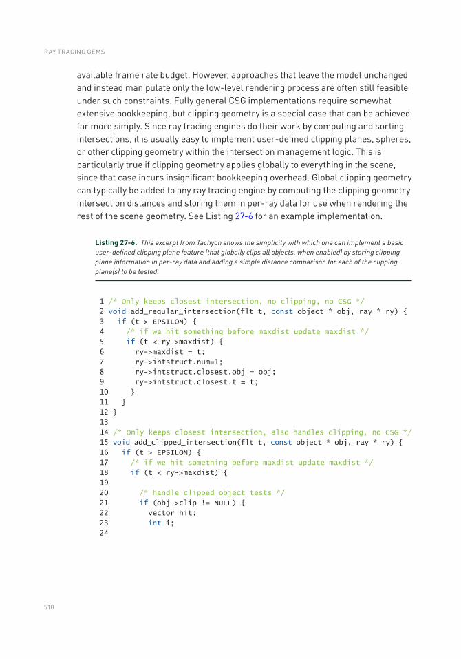
510
available frame rate budget. However, approaches that leave the model unchanged and instead manipulate only the low-level rendering process are often still feasible under such constraints. Fully general CSG implementations require somewhat extensive bookkeeping, but clipping geometry is a special case that can be achieved far more simply. Since ray tracing engines do their work by computing and sorting intersections, it is usually easy to implement user- defined clipping planes, spheres, or other clipping geometry within the intersection management logic. This is particularly true if clipping geometry applies globally to everything in the scene, since that case incurs insignificant bookkeeping overhead. Global clipping geometry can typically be added to any ray tracing engine by computing the clipping geometry intersection distances and storing them in per-ray data for use when rendering the rest of the scene geometry. See Listing 27-6 for an example implementation.
Listing 27-6. This excerpt from Tachyon shows the simplicity with which one can implement a basic user-defined clipping plane feature (that globally clips all objects, when enabled) by storing clipping plane information in per-ray data and adding a simple distance comparison for each of the clipping plane(s) to be tested.
1 /* Only keeps closest intersection, no clipping, no CSG */
2 void add_regular_intersection(flt t, const object * obj, ray * ry)
3 if (t > EPSILON)
4 /* if we hit something before maxdist update maxdist */
5 if (t < ry->maxdist)
6 ry->maxdist = t;
7 ry->intstruct.num=1;
8 ry->intstruct.closest.obj = obj;
9 ry->intstruct.closest.t = t;
10
11
12
13
14 /* Only keeps closest intersection, also handles clipping, no CSG */
15 void add_clipped_intersection(flt t, const object * obj, ray * ry)
16 if (t > EPSILON)
17 /* if we hit something before maxdist update maxdist */
18 if (t < ry->maxdist)
19
20 /* handle clipped object tests */
21 if (obj->clip != NULL)
22 vector hit;
23 int i;
24
RAY TRACING GEMS
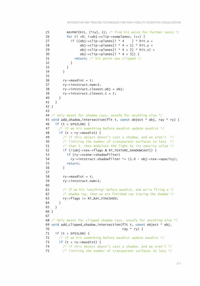
511
25 RAYPNT(hit, (*ry), t); /* find hit point for further tests */
26 for (i =0; i<obj->clip->numplanes; i++)
27 if ((obj->clip->planes[i * 4 ] * hit.x +
28 obj->clip->planes[i * 4 + 1] * hit.y +
29 obj->clip->planes[i * 4 + 2] * hit.z) >
30 obj->clip->planes[i * 4 + 3])
31 return; /* hit point was clipped */
32
33
34
35
36 ry->maxdist = t;
37 ry->intstruct.num=1;
38 ry->intstruct.closest.obj = obj;
39 ry->intstruct.closest.t = t;
40
41
42
43
44 /* Only meant for shadow rays, unsafe for anything else */
45 void add_shadow_intersection(flt t, const object * obj, ray * ry)
46 if (t > EPSILON)
47 /* if we hit something before maxdist update maxdist */
48 if (t < ry->maxdist)
49 /* if this object doesn't cast a shadow, and we aren't */
50 /* limiting the number of transparent surfaces to less */
51 /* than 5, then modulate the light by its opacity value */
52 if (!(obj->tex->flags & RT_TEXTURE_SHADOWCAST))
53 if (ry->scene->shadowfilter)
54 ry->intstruct.shadowfilter *= (1.0 - obj->tex->opacity);
55 return;
56
57
58 ry->maxdist = t;
59 ry->intstruct.num=1;
60
61 /* if we hit *anything* before maxdist, and we're firing a */
62 /* shadow ray, then we are finished ray tracing the shadow */
63 ry->flags |= RT_RAY_FINISHED;
64
65
66
67
68 /* Only meant for clipped shadow rays, unsafe for anything else */
69 void add_clipped_shadow_intersection(flt t, const object * obj,
70 ray * ry)
71 if (t > EPSILON)
72 /* if we hit something before maxdist update maxdist */
73 if (t < ry->maxdist)
74 /* if this object doesn't cast a shadow, and we aren't */
75 /* limiting the number of transparent surfaces to less */
INTERACTIVE RAY TRACING TECHNIQUES FOR HIGH- FIDELITY SCIENTIFIC VISUALIZATION
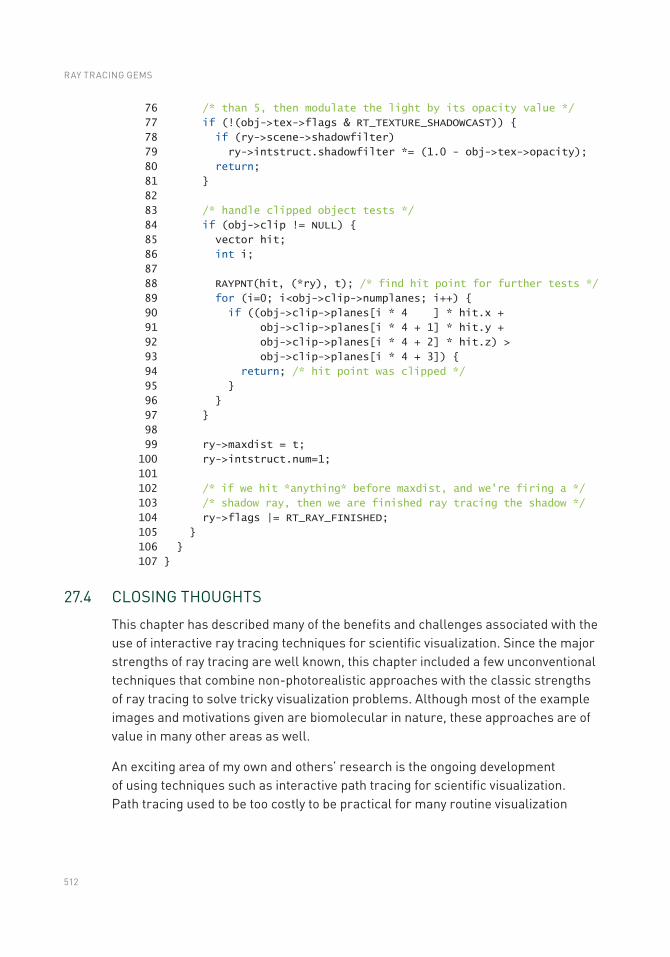
512
76 /* than 5, then modulate the light by its opacity value */
77 if (!(obj->tex->flags & RT_TEXTURE_SHADOWCAST))
78 if (ry->scene->shadowfilter)
79 ry->intstruct.shadowfilter *= (1.0 - obj->tex->opacity);
80 return;
81
82
83 /* handle clipped object tests */
84 if (obj->clip != NULL)
85 vector hit;
86 int i;
87
88 RAYPNT(hit, (*ry), t); /* find hit point for further tests */
89 for (i=0; i<obj->clip->numplanes; i++)
90 if ((obj->clip->planes[i * 4 ] * hit.x +
91 obj->clip->planes[i * 4 + 1] * hit.y +
92 obj->clip->planes[i * 4 + 2] * hit.z) >
93 obj->clip->planes[i * 4 + 3])
94 return; /* hit point was clipped */
95
96
97
98
99 ry->maxdist = t;
100 ry->intstruct.num=1;
101
102 /* if we hit *anything* before maxdist, and we're firing a */
103 /* shadow ray, then we are finished ray tracing the shadow */
104 ry->flags |= RT_RAY_FINISHED;
105
106
107
27.4 CLOSING THOUGHTS
This chapter has described many of the benefits and challenges associated with the use of interactive ray tracing techniques for scientific visualization. Since the major strengths of ray tracing are well known, this chapter included a few unconventional techniques that combine non-photorealistic approaches with the classic strengths of ray tracing to solve tricky visualization problems. Although most of the example images and motivations given are biomolecular in nature, these approaches are of value in many other areas as well.
An exciting area of my own and others’ research is the ongoing development of using techniques such as interactive path tracing for scientific visualization. Path tracing used to be too costly to be practical for many routine visualization
RAY TRACING GEMS
513
tasks that a scientist might perform on a daily basis. However, when the ray tracing performance provided by state-of-the-art hardware is combined with the latest techniques for Monte Carlo image denoising, interactive path tracing becomes feasible for a wide spectrum of visualization workloads without having to compromise on either interactivity or image quality. These developments are of particular value for scientific and technical visualizations where improved photorealism is important.
The code examples provided with the chapter are intended to serve as exemplary starting points for further specialization. Each of the techniques can be significantly extended to add new capabilities far beyond what is demonstrated here, and I have tried to strike a balance between simplicity, reusability, and completeness.
ACKNOWLEDGMENTS
This work was supported in part by the National Institutes of Health, under grant P41-GM104601. The author thanks Melih Sener and Angela Barragan for the use of the chromatophore models. The author wishes to thank many current and former colleagues in the Theoretical and Computational Biophysics Group at the University of Illinois for years of collaboration on the design of the VMD molecular visualization software and the use of advanced rendering techniques for production of effective visualizations.
REFERENCES
[1] Borkiewicz, K., Christensen, A. J., and Stone, J. E. Communicating Science Through Visualization in an Age of Alternative Facts. In ACM SIGGRAPH Courses (2017), pp. 8:1–8:204.
[2] Brownlee, C., Patchett, J., Lo, L.-T., DeMarle, D., Mitchell, C., Ahrens, J., and Hansen, C. D. A Study of Ray Tracing Large-Scale Scientific Data in Two Widely Used Parallel Visualization Applications. In Eurographics Symposium on Parallel Graphics and Visualization (2012), pp. 51–60.
[3] Chaitanya, C. R. A., Kaplanyan, A. S., Schied, C., Salvi, M., Lefohn, A., Nowrouzezahrai, D., and Aila, T. Interactive Reconstruction of Monte Carlo Image Sequences Using a Recurrent Denoising Autoencoder. ACM Transactions on Graphics 36, 4 (July 2017), 98:1–98:12.
[4] Cigolle, Z. H., Donow, S., Evangelakos, D., Mara, M., McGuire, M., and Meyer, Q. A Survey of Efficient Representations for Independent Unit Vectors. Journal of Computer Graphics Techniques 3, 2 (April 2014), 1–30.
[5] Humphrey, W., Dalke, A., and Schulten, K. VMD—Visual Molecular Dynamics. Journal of Molecular Graphics 14, 1 (1996), 33–38.
[6] Kalantari, N. K., Bako, S., and Sen, P. A Machine Learning Approach for Filtering Monte Carlo Noise. ACM Transactions on Graphics 34, 4 (July 2015), 122:1–122:12.
INTERACTIVE RAY TRACING TECHNIQUES FOR HIGH- FIDELITY SCIENTIFIC VISUALIZATION
514
[7] Knoll, A., Wald, I., Navrátil, P. A., Papka, M. E., and Gaither, K. P. Ray Tracing and Volume Rendering Large Molecular Data on Multi-Core and Many-Core Architectures. In International Workshop on Ultrascale Visualization (2013), pp. 5:1–5:8.
[8] Lindstrom, P. Fixed-Rate Compressed Floating-Point Arrays. IEEE Transactions on Visualization and Computer Graphics 20, 12 (Dec. 2014), 2674–2683.
[9] Lindstrom, P., and Isenburg, M. Fast and Efficient Compression of Floating-Point Data. IEEE Transactions on Visualization and Computer Graphics 12, 5 (Sept. 2006), 1245–1250.
[10] Mara, M., McGuire, M., Bitterli, B., and Jarosz, W. An Efficient Denoising Algorithm for Global Illumination. In Proceedings of High-Performance Graphics (2017), pp. 3:1–3:7.
[11] Merritt, E. A., and Murphy, M. E. P. Raster3D Version 2.0—A Program for Photorealistic Molecular Graphics. Acta Crystallography 50, 6 (1994), 869–873.
[12] Meyer, Q., Süßmuth, J., Sußner, G., Stamminger, M., and Greiner, G. On Floating- Point Normal Vectors. In Eurographics Symposium on Rendering (2010), pp. 1405–1409.
[13] Parker, S. G., Bigler, J., Dietrich, A., Friedrich, H., Hoberock, J., Luebke, D., McAllister, D., McGuire, M., Morley, K., Robison, A., and Stich, M. OptiX: A General Purpose Ray Tracing Engine. ACM Transactions on Graphics 29, 4 (2010), 66:1–66:13.
[14] Roth, S. D. Ray Casting for Modeling Solids. Computer Graphics and Image Processing 18, 2 (1982), 109–144.
[15] Santos, J. D., Sen, P., and Oliveira, M. M. A Framework for Developing and Benchmarking Sampling and Denoising Algorithms for Monte Carlo Rendering. The Visual Computer 34, 6-8 (June 2018), 765–778.
[16] Schied, C., Kaplanyan, A., Wyman, C., Patney, A., Chaitanya, C. R. A., Burgess, J., Liu, S., Dachsbacher, C., Lefohn, A., and Salvi, M. Spatiotemporal Variance- Guided Filtering: Real-Time Reconstruction for Path-Traced Global Illumination. In Proceedings of High-Performance Graphics (2017), pp. 2:1–2:12.
[17] Sener, M., Stone, J. E., Barragan, A., Singharoy, A., Teo, I., Vandivort, K. L., Isralewitz, B., Liu, B., Goh, B. C., Phillips, J. C., Kourkoutis, L. F., Hunter, C. N., and Schulten, K. Visualization of Energy Conversion Processes in a Light Harvesting Organelle at Atomic Detail. In International Conference on High Performance Computing, Networking, Storage and Analysis (2014).
[18] Stone, J. E. An Efficient Library for Parallel Ray Tracing and Animation. Master’s thesis, Computer Science Department, University of Missouri-Rolla, April 1998.
[19] Stone, J. E., Isralewitz, B., and Schulten, K. Early Experiences Scaling VMD Molecular Visualization and Analysis Jobs on Blue Waters. In Extreme Scaling Workshop (Aug. 2013), pp. 43–50.
[20] Stone, J. E., Sener, M., Vandivort, K. L., Barragan, A., Singharoy, A., Teo, I., Ribeiro, J. V., Isralewitz, B., Liu, B., Goh, B. C., Phillips, J. C., MacGregor-Chatwin, C., Johnson, M. P., Kourkoutis, L. F., Hunter, C. N., and Schulten, K. Atomic Detail Visualization of Photosynthetic Membranes with GPU-Accelerated Ray Tracing. Parallel Computing 55 (2016), 17–27.
RAY TRACING GEMS
515
[21] Stone, J. E., Sherman, W. R., and Schulten, K. Immersive Molecular Visualization with Omnidirectional Stereoscopic Ray Tracing and Remote Rendering. In IEEE International Parallel and Distributed Processing Symposium Workshop (2016), pp. 1048–1057.
[22] Stone, J. E., Vandivort, K. L., and Schulten, K. GPU-Accelerated Molecular Visualization on Petascale Supercomputing Platforms. In International Workshop on Ultrascale Visualization (2013), pp. 6:1–6:8.
[23] Van Wijk, J. J. Ray Tracing Objects Defined by Sweeping a Sphere. Computers & Graphics 9, 3 (1985), 283–290.
[24] Wald, I., Friedrich, H., Knoll, A., and Hansen, C. Interactive Isosurface Ray Tracing of Time-Varying Tetrahedral Volumes. IEEE Transactions on Visualization and Computer Graphics 13, 6 (11 2007), 1727–1734.
[25] Wald, I., Johnson, G., Amstutz, J., Brownlee, C., Knoll, A., Jeffers, J., Gunther, J., and Navratil, P. OSPRay—A CPU Ray Tracing Framework for Scientific Visualization. IEEE Transactions on Visualization and Computer Graphics 23, 1 (2017), 931–940.
[26] Wald, I., Woop, S., Benthin, C., Johnson, G. S., and Ernst, M. Embree: A Kernel Framework for Efficient CPU Ray Tracing. ACM Transactions on Graphics 33, 4 (July 2014), 143:1–143:8.
Open Access This chapter is licensed under the terms of the Creative Commons Attribution-NonCommercial-NoDerivatives 4.0 International License (http://creativecommons.org/licenses/by-nc-nd/4.0/), which permits any noncommercial use, sharing, distribution and
reproduction in any medium or format, as long as you give appropriate credit to the original author(s) and the source, provide a link to the Creative Commons license and indicate if you modified the licensed material. You do not have permission under this license to share adapted material derived from this chapter or parts of it.
The images or other third party material in this chapter are included in the chapter's Creative Commons license, unless indicated otherwise in a credit line to the material. If material is not included in the chapter's Creative Commons license and your intended use is not permitted by statutory regulation or exceeds the permitted use, you will need to obtain permission directly from the copyright holder.
INTERACTIVE RAY TRACING TECHNIQUES FOR HIGH- FIDELITY SCIENTIFIC VISUALIZATION
PART VII
GLOBAL ILLUMINATION
519
PART VII
Global Illumination
Lighting in the real world is remarkably complex, in large part due to multiply scattered light—photons that leave a light source, bounce off other non-emissive surfaces, and indirectly illuminate objects in the scene. Modeling this lighting effect, known as global illumination, greatly contributes to the realism of rendered images, as it is something that we are used to seeing all the time in the real world.
Since the introduction of programmable GPUs almost 20 years ago, developers have worked to develop real-time global illumination algorithms. While there has been great innovation, it has been hampered by GPUs that, until recently, offered only rasterization as a visibility algorithm. The challenge with global illumination is that the visibility queries that one would like to make are highly incoherent, point-to-point tests—not at all a good fit for a rasterizer.
With the introduction of RTX GPUs, ray tracing is now available in the real-time graphics pipeline. Of course, having this capability does not make everything easy: one still has to choose one’s rays carefully, use clever algorithms, and consider denoising. This part includes five chapters that describe cutting-edge work in ray tracing for global illumination, all of it well suited to GPU rendering.
Chapter 28, “Ray Tracing Inhomogeneous Volumes,” is about rendering volumetric scattering with ray tracing. It describes key techniques for rendering clouds, smoke, and explosions, with an approach that integrates cleanly into surface ray tracing. A full implementation of the algorithms described is included.
While not strictly related to global illumination, Chapter 29, “Efficient Particle Volume Splatting in a Ray Tracer,” concerns rendering hundreds of million particles efficiently, using ray tracing instead of rasterization. The technique could also be applied to ray tracing all sorts of other complex scattering effects from many small particles.
Chapter 30, “Caustics Using Screen-Space Photon Mapping,” is entirely focused on caustics, the often beautiful light patterns that result from light reflecting or refracting from curved surfaces. It explains how to render them using photon mapping, a technique based on tracing light particles from emitters and then using their local density at points being shaded to estimate caustics there.
520
With modern light transport algorithms, mathematical innovation can be just as important as code optimization and performance. Chapter 31, “Variance Reduction via Footprint Estimation in the Presence of Path Reuse,” considers the task of weighting light-carrying paths when using hybrid light transport algorithms that combine bidirectional path tracing and photon mapping, introducing a new approach to this problem.
This part (and this book) concludes with Chapter 32, “Accurate Real-Time Specular Reflections with Radiance Caching,” which describes a technique to accurately render glossy specular reflections that combines ray tracing from specular surfaces—to accurately compute points that they reflect—and cube map radiance probes—as an efficient approximation of their reflected light.
Enjoy these chapters, all of which are undeniably illuminating. The many interesting ideas that they present will almost certainly be useful in the rendering challenges that you face in the future.
Matt Pharr
521© NVIDIA 2019 E. Haines, T. Akenine-Möller (eds.), Ray Tracing Gems, https://doi.org/10.1007/978-1-4842-4427-2_28
CHAPTER 28
Ray Tracing Inhomogeneous VolumesMatthias RaabNVIDIA
ABSTRACT
Simulating the interaction of light with scattering and absorbing media requires importance sampling of distances proportional to the volume transmittance. A simple method originating from neutron transport simulation can be used to importance- sample collision events of a particle like a photon with arbitrary media.
28.1 LIGHT TRANSPORT IN VOLUMES
When light passes through a volume along a ray, some of it may be scattered or absorbed according to the medium’s light interaction properties. This is modeled by the medium’s scattering coefficient σ and absorption coefficient α. Generally, both are functions that vary with position. Adding the two, we obtain the extinction coefficient κ = σ + α, which characterizes total loss due to (out-)scattering and absorption.
The ratio of light that is not scattered out or absorbed for a distance s is called volume transmittance T and is described by the Beer-Lambert Law: if we follow a ray starting at position o in direction d, transmittance is
( ) ( )
0exp .
ST , s t dtkòæ ö+ = - +ç ÷
è øo o d o d
(1)
This term is prominently featured in the integral equations governing light transport. For example, the radiance scattered in along a ray for distance s is given by integrating the transmittance-weighted in-scattered radiance (according to scattering coefficient σs and phase function fp):
( ) ( ) ( )
0( ) .
S
s pL , T , t , t f t , , d dts w wò òW
æ ö- = + + + -ç ÷è ø
o d o o d o o d o d d
(2)
522
A Monte Carlo path tracer will typically want to importance-sample a distance proportional to T. The physical interpretation is that one would stochastically simulate the distance at which an interaction occurs for a photon. The path tracer can then randomly decide if the event is absorption or scattering and, in case of the latter, continue to trace the photon into a direction sampled according to the phase function. The probability density proportional to T is
( ) ( ) ( ) ( ) ( )
0exp .
tp t t T , t t t dtk k kòæ ö= + + = + - +ç ÷
è ø¢ ¢o d o o d o d o d (3)
In cases where the medium is homogeneous (i.e., κ is constant), this simplifies to an exponential distribution κe−κt and the inversion method can be applied to obtain the distance
( )t ln 1 / ,x k= - - (4)
with the desired distribution for a uniformly distributed ξ. For an inhomogenous medium, however, this will not work, since for general κ the integral in Equation 3 cannot be solved analytically, or even if so, the inverse might not be available.
28.2 WOODCOCK TRACKING
In the context of tracking the trajectories of neutrons (where one deals with the same sort of equations as with photons), a technique to importance-sample distances in inhomogeneous media found widespread use in the 1960s. It is often called Woodcock tracking, referring to a publication by Woodcock et al. [5]
The idea is quite simple and based on the fact that homogeneous volumes can be handled easily. To obtain an artificial homogeneous setting, a fictitious extinction coefficient is added such that the sum of the actual and the fictitious extinctions equals the maximum κmax everywhere. The artificial volume can now be interpreted as a mix of actual particles, which actually scatter and absorb, and the fictitious ones that will not do anything. See Figure 28-1.
RAY TRACING GEMS
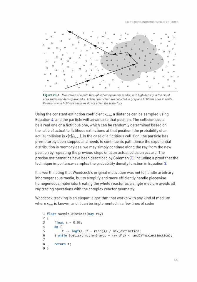
523
Using the constant extinction coefficient κmax, a distance can be sampled using Equation 4, and the particle will advance to that position. The collision could be a real one or a fictitious one, which can be randomly determined based on the ratio of actual to fictitious extinctions at that position (the probability of an actual collision is κ(x)/κmax). In the case of a fictitious collision, the particle has prematurely been stopped and needs to continue its path. Since the exponential distribution is memoryless, we may simply continue along the ray from the new position by repeating the previous steps until an actual collision occurs. The precise mathematics have been described by Coleman [1], including a proof that the technique importance-samples the probability density function in Equation 3.
It is worth noting that Woodcock’s original motivation was not to handle arbitrary inhomogeneous media, but to simplify and more efficiently handle piecewise homogeneous materials: treating the whole reactor as a single medium avoids all ray tracing operations with the complex reactor geometry.
Woodcock tracking is an elegant algorithm that works with any kind of medium where κmax is known, and it can be implemented in a few lines of code:
1 float sample_distance(Ray ray)
2
3 float t = 0.0f;
4 do
5 t -= logf(1.0f - rand()) / max_extinction;
6 while (get_extinction(ray.o + ray.d*t) < rand()*max_extinction);
7
8 return t;
9
Figure 28-1. Illustration of a path through inhomogeneous media, with high density in the cloud area and lower density around it. Actual “particles” are depicted in gray and fictitious ones in white. Collisions with fictitious particles do not affect the trajectory.
RAy TRACING INHOMOGENEOUS VOLUMES
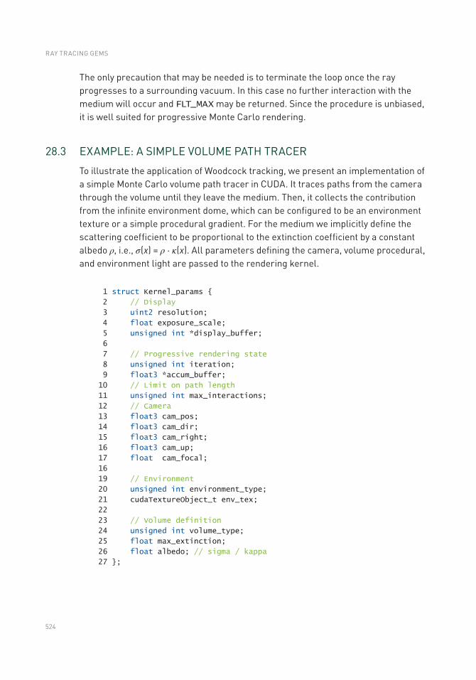
524
The only precaution that may be needed is to terminate the loop once the ray progresses to a surrounding vacuum. In this case no further interaction with the medium will occur and FLT_MAX may be returned. Since the procedure is unbiased, it is well suited for progressive Monte Carlo rendering.
28.3 EXAMPLE: A SIMPLE VOLUME PATH TRACER
To illustrate the application of Woodcock tracking, we present an implementation of a simple Monte Carlo volume path tracer in CUDA. It traces paths from the camera through the volume until they leave the medium. Then, it collects the contribution from the infinite environment dome, which can be configured to be an environment texture or a simple procedural gradient. For the medium we implicitly define the scattering coefficient to be proportional to the extinction coefficient by a constant albedo ρ, i.e., σ(x) = ρ ⋅ κ(x). All parameters defining the camera, volume procedural, and environment light are passed to the rendering kernel.
1 struct Kernel_params
2 // Display
3 uint2 resolution;
4 float exposure_scale;
5 unsigned int *display_buffer;
6
7 // Progressive rendering state
8 unsigned int iteration;
9 float3 *accum_buffer;
10 // Limit on path length
11 unsigned int max_interactions;
12 // Camera
13 float3 cam_pos;
14 float3 cam_dir;
15 float3 cam_right;
16 float3 cam_up;
17 float cam_focal;
16
19 // Environment
20 unsigned int environment_type;
21 cudaTextureObject_t env_tex;
22
23 // Volume definition
24 unsigned int volume_type;
25 float max_extinction;
26 float albedo; // sigma / kappa
27 ;
RAY TRACING GEMS
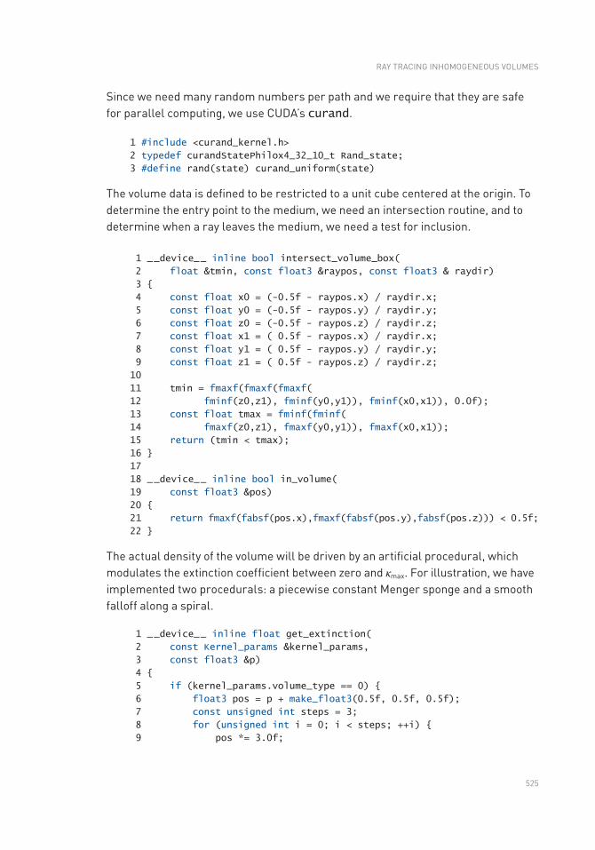
525
Since we need many random numbers per path and we require that they are safe for parallel computing, we use CUDA’s curand.
1 #include <curand_kernel.h>
2 typedef curandStatePhilox4_32_10_t Rand_state;
3 #define rand(state) curand_uniform(state)
The volume data is defined to be restricted to a unit cube centered at the origin. To determine the entry point to the medium, we need an intersection routine, and to determine when a ray leaves the medium, we need a test for inclusion.
1 _ _device_ _ inline bool intersect_volume_box(
2 float &tmin, const float3 &raypos, const float3 & raydir)
3
4 const float x0 = (-0.5f - raypos.x) / raydir.x;
5 const float y0 = (-0.5f - raypos.y) / raydir.y;
6 const float z0 = (-0.5f - raypos.z) / raydir.z;
7 const float x1 = ( 0.5f - raypos.x) / raydir.x;
8 const float y1 = ( 0.5f - raypos.y) / raydir.y;
9 const float z1 = ( 0.5f - raypos.z) / raydir.z;
10
11 tmin = fmaxf(fmaxf(fmaxf(
12 fminf(z0,z1), fminf(y0,y1)), fminf(x0,x1)), 0.0f);
13 const float tmax = fminf(fminf(
14 fmaxf(z0,z1), fmaxf(y0,y1)), fmaxf(x0,x1));
15 return (tmin < tmax);
16
17
18 _ _device_ _ inline bool in_volume(
19 const float3 &pos)
20
21 return fmaxf(fabsf(pos.x),fmaxf(fabsf(pos.y),fabsf(pos.z))) < 0.5f;
22
The actual density of the volume will be driven by an artificial procedural, which modulates the extinction coefficient between zero and κmax. For illustration, we have implemented two procedurals: a piecewise constant Menger sponge and a smooth falloff along a spiral.
1 _ _device_ _ inline float get_extinction(
2 const Kernel_params &kernel_params,
3 const float3 &p)
4
5 if (kernel_params.volume_type == 0)
6 float3 pos = p + make_float3(0.5f, 0.5f, 0.5f);
7 const unsigned int steps = 3;
8 for (unsigned int i = 0; i < steps; ++i)
9 pos *= 3.0f;
RAy TRACING INHOMOGENEOUS VOLUMES
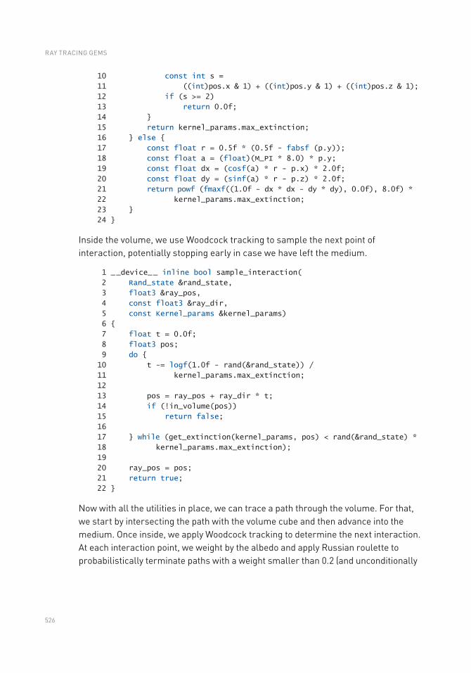
526
10 const int s =
11 ((int)pos.x & 1) + ((int)pos.y & 1) + ((int)pos.z & 1);
12 if (s >= 2)
13 return 0.0f;
14
15 return kernel_params.max_extinction;
16 else
17 const float r = 0.5f * (0.5f - fabsf (p.y));
18 const float a = (float)(M_PI * 8.0) * p.y;
19 const float dx = (cosf(a) * r - p.x) * 2.0f;
20 const float dy = (sinf(a) * r - p.z) * 2.0f;
21 return powf (fmaxf((1.0f - dx * dx - dy * dy), 0.0f), 8.0f) *
22 kernel_params.max_extinction;
23
24
Inside the volume, we use Woodcock tracking to sample the next point of interaction, potentially stopping early in case we have left the medium.
1 _ _device_ _ inline bool sample_interaction(
2 Rand_state &rand_state,
3 float3 &ray_pos,
4 const float3 &ray_dir,
5 const Kernel_params &kernel_params)
6
7 float t = 0.0f;
8 float3 pos;
9 do
10 t -= logf(1.0f - rand(&rand_state)) /
11 kernel_params.max_extinction;
12
13 pos = ray_pos + ray_dir * t;
14 if (!in_volume(pos))
15 return false;
16
17 while (get_extinction(kernel_params, pos) < rand(&rand_state) *
18 kernel_params.max_extinction);
19
20 ray_pos = pos;
21 return true;
22
Now with all the utilities in place, we can trace a path through the volume. For that, we start by intersecting the path with the volume cube and then advance into the medium. Once inside, we apply Woodcock tracking to determine the next interaction. At each interaction point, we weight by the albedo and apply Russian roulette to probabilistically terminate paths with a weight smaller than 0.2 (and unconditionally
RAY TRACING GEMS
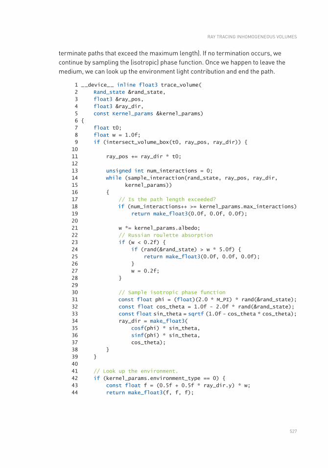
527
terminate paths that exceed the maximum length). If no termination occurs, we continue by sampling the (isotropic) phase function. Once we happen to leave the medium, we can look up the environment light contribution and end the path.
1 _ _device_ _ inline float3 trace_volume(
2 Rand_state &rand_state,
3 float3 &ray_pos,
4 float3 &ray_dir,
5 const Kernel_params &kernel_params)
6
7 float t0;
8 float w = 1.0f;
9 if (intersect_volume_box(t0, ray_pos, ray_dir))
10
11 ray_pos += ray_dir * t0;
12
13 unsigned int num_interactions = 0;
14 while (sample_interaction(rand_state, ray_pos, ray_dir,
15 kernel_params))
16
17 // Is the path length exceeded?
18 if (num_interactions++ >= kernel_params.max_interactions)
19 return make_float3(0.0f, 0.0f, 0.0f);
20
21 w *= kernel_params.albedo;
22 // Russian roulette absorption
23 if (w < 0.2f)
24 if (rand(&rand_state) > w * 5.0f)
25 return make_float3(0.0f, 0.0f, 0.0f);
26
27 w = 0.2f;
28
29
30 // Sample isotropic phase function
31 const float phi = (float)(2.0 * M_PI) * rand(&rand_state);
32 const float cos_theta = 1.0f - 2.0f * rand(&rand_state);
33 const float sin_theta = sqrtf (1.0f - cos_theta * cos_theta);
34 ray_dir = make_float3(
35 cosf(phi) * sin_theta,
36 sinf(phi) * sin_theta,
37 cos_theta);
38
39
40
41 // Look up the environment.
42 if (kernel_params.environment_type == 0)
43 const float f = (0.5f + 0.5f * ray_dir.y) * w;
44 return make_float3(f, f, f);
RAy TRACING INHOMOGENEOUS VOLUMES
528
45 else
46 const float4 texval = tex2D<float4>(
47 kernel_params.env_tex,
48 atan2f(ray_dir.z, ray_dir.x) * (float)(0.5 / M_PI) + 0.5f,
49 acosf(fmaxf(fminf(ray_dir.y, 1.0f), -1.0f)) *
50 (float)(1.0 / M_PI));
51 return make_float3(texval.x * w, texval.y * w, texval.z * w);
52
53
Finally, we add the logic to start paths from the camera for each pixel. The results are progressively accumulated and transferred to a tone-mapped buffer for display after each iteration.
1 extern "C" _ _global_ _ void volume_rt_kernel(
2 const Kernel_params kernel_params)
3
4 const unsigned int x = blockIdx.x * blockDim.x + threadIdx.x;
5 const unsigned int y = blockIdx.y * blockDim.y + threadIdx.y;
6 if (x >= kernel_params.resolution.x ||
7 y >= kernel_params.resolution.y)
8 return;
9
10 // Initialize pseudorandom number generator (PRNG);
11 // assume we need no more than 4096 random numbers.
12 const unsigned int idx = y * kernel_params.resolution.x + x;
13 Rand_state rand_state;
14 curand_init(idx, 0, kernel_params.iteration * 4096, &rand_state);
15
16 // Trace from the pinhole camera.
17 const float inv_res_x = 1.0f / (float)kernel_params.resolution.x;
18 const float inv_res_y = 1.0f / (float)kernel_params.resolution.y;
19 const float pr = (2.0f * ((float)x + rand(&rand_state)) * inv_res_x
20 - 1.0f);
21 const float pu = (2.0f * ((float)y + rand(&rand_state)) * inv_res_y
22 - 1.0f);
23 const float aspect = (float)kernel_params.resolution.y * inv_res_x;
24 float3 ray_pos = kernel_params.cam_pos;
25 float3 ray_dir = normalize(
26 kernel_params.cam_dir * kernel_params.cam_focal +
27 kernel_params.cam_right * pr +
28 kernel_params.cam_up * aspect * pu);
29 const float3 value = trace_volume(rand_state, ray_pos, ray_dir,
30 kernel_params);
31
RAY TRACING GEMS
529
32 // Accumulate.
33 if (kernel_params.iteration == 0)
34 kernel_params.accum_buffer[idx] = value;
35 else
36 kernel_params.accum_buffer[idx] =
37 kernel_params.accum_buffer[idx] +
38 (value - kernel_params.accum_buffer[idx]) /
39 (float)(kernel_params.iteration + 1);
40
41 // Update display buffer (simple Reinhard tone mapper + gamma).
42 float3 val = kernel_params.accum_buffer[idx] *
43 kernel_params.exposure_scale;
44 val.x *= (1.0f + val.x * 0.1f) / (1.0f + val.x);
45 val.y *= (1.0f + val.y * 0.1f) / (1.0f + val.y);
46 val.z *= (1.0f + val.z * 0.1f) / (1.0f + val.z);
47 const unsigned int r = (unsigned int)(255.0f *
48 fminf(powf(fmaxf(val.x, 0.0f), (float)(1.0 / 2.2)), 1.0f));
49 const unsigned int g = (unsigned int) (255.0f *
50 fminf(powf(fmaxf(val.y, 0.0f), (float)(1.0 / 2.2)), 1.0f));
51 const unsigned int b = (unsigned int) (255.0f *
52 fminf(powf(fmaxf(val.z, 0.0f), (float)(1.0 / 2.2)), 1.0f));
53 kernel_params.display_buffer[idx] =
54 0xff000000 | (r << 16) | (g << 8) | b;
55
Example renderings produced by the presented path tracer can be seen in Figure 28- 2.
RAy TRACING INHOMOGENEOUS VOLUMES
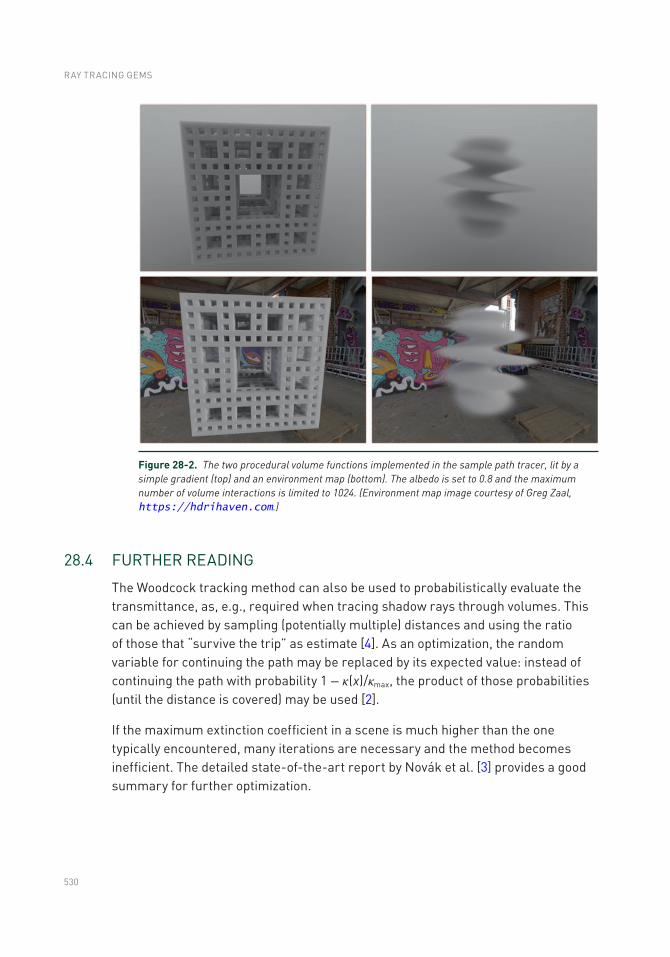
530
28.4 FURTHER READING
The Woodcock tracking method can also be used to probabilistically evaluate the transmittance, as, e.g., required when tracing shadow rays through volumes. This can be achieved by sampling (potentially multiple) distances and using the ratio of those that “survive the trip” as estimate [4]. As an optimization, the random variable for continuing the path may be replaced by its expected value: instead of continuing the path with probability 1 − κ(x)/κmax, the product of those probabilities (until the distance is covered) may be used [2].
If the maximum extinction coefficient in a scene is much higher than the one typically encountered, many iterations are necessary and the method becomes inefficient. The detailed state-of-the-art report by Novák et al. [3] provides a good summary for further optimization.
Figure 28-2. The two procedural volume functions implemented in the sample path tracer, lit by a simple gradient (top) and an environment map (bottom). The albedo is set to 0.8 and the maximum number of volume interactions is limited to 1024. (Environment map image courtesy of Greg Zaal, https://hdrihaven.com.)
RAY TRACING GEMS
531
REFERENCES
[1] Coleman, W. Mathematical Verification of a Certain Monte Carlo Sampling Technique and Applications of the Technique to Radiation Transport Problems. Nuclear Science and Engineering 32 (1968), 76–81.
[2] Novák, J., Selle, A., and Jarosz, W. Residual Ratio Tracking for Estimating Attenuation in Participating Media. ACM Transactions on Graphics (SIGGRAPH Asia) 33, 6 (Nov. 2014), 179:1–179:11.
[3] Novák, J., Georgiev, I., Hanika, J., and Jarosz, W. Monte Carlo Methods for Volumetric Light Transport Simulation. Computer Graphics Forum 37, 2 (May 2018), 551–576.
[4] Raab, M., Seibert, D., and Keller, A. Unbiased Global Illumination with Participating Media. In Monte Carlo and Quasi-Monte Carlo Methods, A. Keller, S. Heinrich, and N. H., Eds. Springer, 2008, pp. 591–605.
[5] Woodcock, E. R., Murphy, T., Hemmings, P. J., and Longworth, T. C. Techniques Used in the GEM Code for Monte Carlo Neutronics Calculations in Reactors and Other Systems of Complex Geometry. In Conference on Applications of Computing Methods to Reactor Problems (1965), pp. 557–579.
Open Access This chapter is licensed under the terms of the Creative Commons Attribution-NonCommercial-NoDerivatives 4.0 International License (http://creativecommons.org/licenses/by-nc-nd/4.0/), which permits any noncommercial use, sharing, distribution and
reproduction in any medium or format, as long as you give appropriate credit to the original author(s) and the source, provide a link to the Creative Commons license and indicate if you modified the licensed material. you do not have permission under this license to share adapted material derived from this chapter or parts of it.
The images or other third party material in this chapter are included in the chapter's Creative Commons license, unless indicated otherwise in a credit line to the material. If material is not included in the chapter's Creative Commons license and your intended use is not permitted by statutory regulation or exceeds the permitted use, you will need to obtain permission directly from the copyright holder.
RAy TRACING INHOMOGENEOUS VOLUMES
533© NVIDIA 2019 E. Haines, T. Akenine-Möller (eds.), Ray Tracing Gems, https://doi.org/10.1007/978-1-4842-4427-2_29
CHAPTER 29
Efficient Particle Volume Splatting in a Ray TracerAaron Knoll, R. Keith Morley, Ingo Wald, Nick Leaf, and Peter Messmer
NVIDIA
ABSTRACT
Rendering of particle data sets is a common problem in many domains including games, film, and scientific visualization. Conventionally, this has been accomplished using rasterization-based splatting methods, which scale linearly with respect to problem size. Given sufficiently low-cost ray traversal with logarithmic complexity, splatting within a ray tracing framework could scale better to larger geometry. In this chapter, we provide a method for efficiently rendering larger particle data, exploiting ray coherence and leveraging hardware-accelerated traversal on architectures such as the NVIDIA RTX 2080 Ti (Turing) GPUs with RT Cores technology.
29.1 MOTIVATION
Rasterization-based GPU splatting approaches generally break down when most primitives have subpixel footprints and when depth sorting is desired. This occurs due to the linear cost of depth-sorting fragments, as well as incoherent framebuffer traffic, and in practice hampers interactive performance for particle counts beyond 20 million depending on the GPU. There are numerous workarounds for faster raster performance including view-dependent spatial subdivision, level of detail, disabling the depth test and alpha blending, or resampling onto a proxy such as texture slices. However, for all of these, performance suffers when one actually renders a sufficiently high number of particles.
One could equally use ray tracing architectures to efficiently traverse and render full particle data. Traversing an acceleration structure generally has logarithmic time complexity; moreover, it can be done in a way that fosters many small, localized primitive sorts instead of a single large sort. In this manner, we wish performance to mirror the number of primitives actually intersected by each ray, not the total complexity of the whole scene. There are other reasons for rendering particle data within a ray tracing framework, for example allowing particle
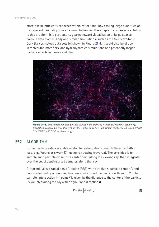
534
effects to be efficiently rendered within reflections. Ray casting large quantities of transparent geometry poses its own challenges; this chapter provides one solution to this problem. It is particularly geared toward visualization of large sparse particle data from N-body and similar simulations, such as the freely available DarkSky cosmology data sets [6] shown in Figure 29-1. It could also be of use in molecular, materials, and hydrodynamics simulations and potentially larger particle effects in games and film.
Figure 29-1. One hundred million particle subset of the DarkSky N-body gravitational cosmology simulation, rendered in its entirety at 35 FPS (1080p) or 14 FPS (4k) without level of detail, on an NVIDIA RTX 2080 Ti with RT Cores technology.
29.2 ALGORITHM
Our aim is to create a scalable analog to rasterization-based billboard splatting (see, e.g., Westover’s work [7]) using ray tracing traversal. The core idea is to sample each particle close to its center point along the viewing ray, then integrate over the set of depth-sorted samples along that ray.
Our primitive is a radial basis function (RBF) with a radius r, particle center P, and bounds defined by a bounding box centered around the particle with width 2r. The sample (intersection hit) point X is given by the distance to the center of the particle P evaluated along the ray with origin O and direction d,
X O P O .= + - d (1)
RAY TRACING GEMS
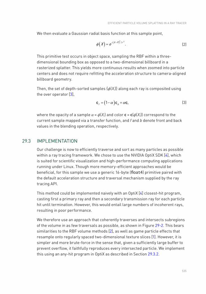
535
We then evaluate a Gaussian radial basis function at this sample point,
( ) ( )X P rX e2 2/ .f - -=
(2)
This primitive test occurs in object space, sampling the RBF within a three- dimensional bounding box as opposed to a two-dimensional billboard in a rasterized splatter. This yields more continuous results when zoomed into particle centers and does not require refitting the acceleration structure to camera-aligned billboard geometry.
Then, the set of depth-sorted samples ϕ(Xi) along each ray is composited using the over operator [3],
( )f b1 ,a a= - +c c c
(3)
where the opacity of a sample α = ϕ(Xi) and color c = c(ϕ(Xi)) correspond to the current sample mapped via a transfer function, and f and b denote front and back values in the blending operation, respectively.
29.3 IMPLEMENTATION
Our challenge is now to efficiently traverse and sort as many particles as possible within a ray tracing framework. We chose to use the NVIDIA OptiX SDK [4], which is suited for scientific visualization and high-performance computing applications running under Linux. Though more memory-efficient approaches would be beneficial, for this sample we use a generic 16-byte (float4) primitive paired with the default acceleration structure and traversal mechanism supplied by the ray tracing API.
This method could be implemented naively with an OptiX [4] closest-hit program, casting first a primary ray and then a secondary transmission ray for each particle hit until termination. However, this would entail large numbers of incoherent rays, resulting in poor performance.
We therefore use an approach that coherently traverses and intersects subregions of the volume in as few traversals as possible, as shown in Figure 29-2. This bears similarities to the RBF volume methods [2], as well as game particle effects that resample onto regularly spaced two-dimensional texture slices [1]. However, it is simpler and more brute-force in the sense that, given a sufficiently large buffer to prevent overflow, it faithfully reproduces every intersected particle. We implement this using an any-hit program in OptiX as described in Section 29.3.2.
EFFICIENT PARTICLE VOLUME SPLATTING IN A RAy TRACER
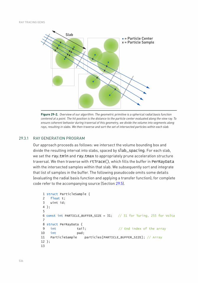
536
29.3.1 RAy GENERATION PROGRAM
Our approach proceeds as follows: we intersect the volume bounding box and divide the resulting interval into slabs, spaced by slab_spacing. For each slab, we set the ray.tmin and ray.tmax to appropriately prune acceleration structure traversal. We then traverse with rtTrace(), which fills the buffer in PerRayData with the intersected samples within that slab. We subsequently sort and integrate that list of samples in the buffer. The following pseudocode omits some details (evaluating the radial basis function and applying a transfer function); for complete code refer to the accompanying source (Section 29.5).
1 struct ParticleSample
2 float t;
3 uint id;
4 ;
5
6 const int PARTICLE_BUFFER_SIZE = 31; // 31 for Turing, 255 for Volta
7
8 struct PerRayData
9 int tail; // End index of the array
10 int pad;
11 ParticleSample particles[PARTICLE_BUFFER_SIZE]; // Array
12 ;
13
Figure 29-2. Overview of our algorithm. The geometric primitive is a spherical radial basis function centered at a point. The hit position is the distance to the particle center evaluated along the view ray. To ensure coherent behavior during traversal of this geometry, we divide the volume into segments along rays, resulting in slabs. We then traverse and sort the set of intersected particles within each slab.
RAY TRACING GEMS
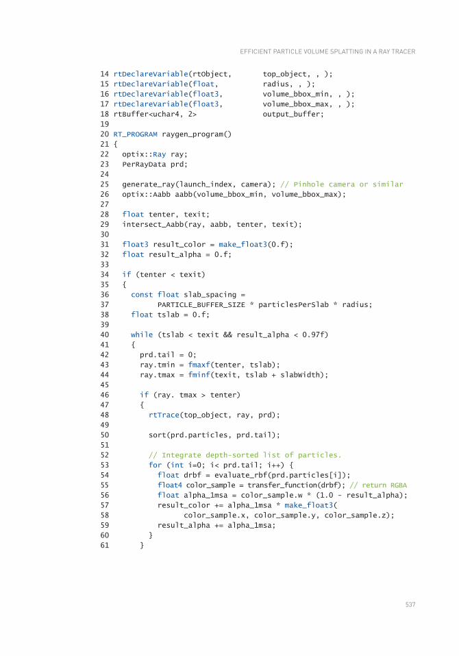
537
14 rtDeclareVariable(rtObject, top_object, , );
15 rtDeclareVariable(float, radius, , );
16 rtDeclareVariable(float3, volume_bbox_min, , );
17 rtDeclareVariable(float3, volume_bbox_max, , );
18 rtBuffer<uchar4, 2> output_buffer;
19
20 RT_PROGRAM raygen_program()
21
22 optix::Ray ray;
23 PerRayData prd;
24
25 generate_ray(launch_index, camera); // Pinhole camera or similar
26 optix::Aabb aabb(volume_bbox_min, volume_bbox_max);
27
28 float tenter, texit;
29 intersect_Aabb(ray, aabb, tenter, texit);
30
31 float3 result_color = make_float3(0.f);
32 float result_alpha = 0.f;
33
34 if (tenter < texit)
35
36 const float slab_spacing =
37 PARTICLE_BUFFER_SIZE * particlesPerSlab * radius;
38 float tslab = 0.f;
39
40 while (tslab < texit && result_alpha < 0.97f)
41
42 prd.tail = 0;
43 ray.tmin = fmaxf(tenter, tslab);
44 ray.tmax = fminf(texit, tslab + slabWidth);
45
46 if (ray. tmax > tenter)
47
48 rtTrace(top_object, ray, prd);
49
50 sort(prd.particles, prd.tail);
51
52 // Integrate depth-sorted list of particles.
53 for (int i=0; i< prd.tail; i++)
54 float drbf = evaluate_rbf(prd.particles[i]);
55 float4 color_sample = transfer_function(drbf); // return RGBA
56 float alpha_1msa = color_sample.w * (1.0 - result_alpha);
57 result_color += alpha_1msa * make_float3(
58 color_sample.x, color_sample.y, color_sample.z);
59 result_alpha += alpha_1msa;
60
61
EFFICIENT PARTICLE VOLUME SPLATTING IN A RAy TRACER
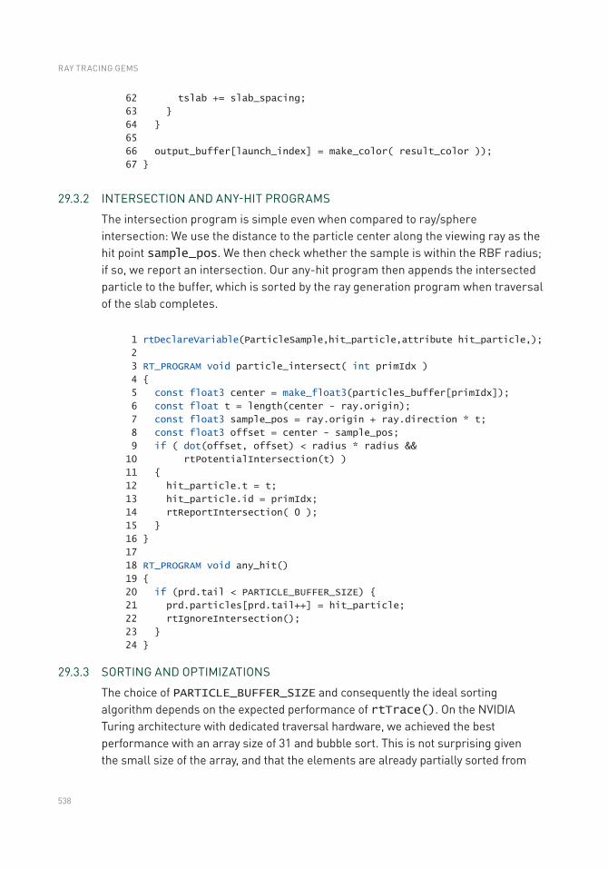
538
62 tslab += slab_spacing;
63
64
65
66 output_buffer[launch_index] = make_color( result_color ));
67
29.3.2 INTERSECTION AND ANy-HIT PROGRAMS
The intersection program is simple even when compared to ray/sphere intersection: We use the distance to the particle center along the viewing ray as the hit point sample_pos. We then check whether the sample is within the RBF radius; if so, we report an intersection. Our any-hit program then appends the intersected particle to the buffer, which is sorted by the ray generation program when traversal of the slab completes.
1 rtDeclareVariable(ParticleSample,hit_particle,attribute hit_particle,);
2
3 RT_PROGRAM void particle_intersect( int primIdx )
4
5 const float3 center = make_float3(particles_buffer[primIdx]);
6 const float t = length(center - ray.origin);
7 const float3 sample_pos = ray.origin + ray.direction * t;
8 const float3 offset = center - sample_pos;
9 if ( dot(offset, offset) < radius * radius &&
10 rtPotentialIntersection(t) )
11
12 hit_particle.t = t;
13 hit_particle.id = primIdx;
14 rtReportIntersection( 0 );
15
16
17
18 RT_PROGRAM void any_hit()
19
20 if (prd.tail < PARTICLE_BUFFER_SIZE)
21 prd.particles[prd.tail++] = hit_particle;
22 rtIgnoreIntersection();
23
24
29.3.3 SORTING AND OPTIMIZATIONS
The choice of PARTICLE_BUFFER_SIZE and consequently the ideal sorting algorithm depends on the expected performance of rtTrace(). On the NVIDIA Turing architecture with dedicated traversal hardware, we achieved the best performance with an array size of 31 and bubble sort. This is not surprising given the small size of the array, and that the elements are already partially sorted from
RAY TRACING GEMS
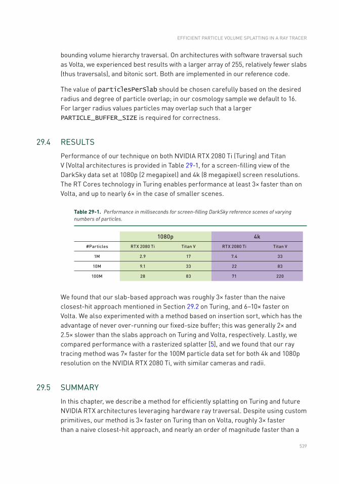
539
bounding volume hierarchy traversal. On architectures with software traversal such as Volta, we experienced best results with a larger array of 255, relatively fewer slabs (thus traversals), and bitonic sort. Both are implemented in our reference code.
The value of particlesPerSlab should be chosen carefully based on the desired radius and degree of particle overlap; in our cosmology sample we default to 16. For larger radius values particles may overlap such that a larger PARTICLE_BUFFER_SIZE is required for correctness.
29.4 RESULTS
Performance of our technique on both NVIDIA RTX 2080 Ti (Turing) and Titan V (Volta) architectures is provided in Table 29-1, for a screen-filling view of the DarkSky data set at 1080p (2 megapixel) and 4k (8 megapixel) screen resolutions. The RT Cores technology in Turing enables performance at least 3× faster than on Volta, and up to nearly 6× in the case of smaller scenes.
Table 29-1. Performance in milliseconds for screen-filling DarkSky reference scenes of varying numbers of particles.
We found that our slab-based approach was roughly 3× faster than the naive closest- hit approach mentioned in Section 29.2 on Turing, and 6–10× faster on Volta. We also experimented with a method based on insertion sort, which has the advantage of never over-running our fixed-size buffer; this was generally 2× and 2.5× slower than the slabs approach on Turing and Volta, respectively. Lastly, we compared performance with a rasterized splatter [5], and we found that our ray tracing method was 7× faster for the 100M particle data set for both 4k and 1080p resolution on the NVIDIA RTX 2080 Ti, with similar cameras and radii.
29.5 SUMMARy
In this chapter, we describe a method for efficiently splatting on Turing and future NVIDIA RTX architectures leveraging hardware ray traversal. Despite using custom primitives, our method is 3× faster on Turing than on Volta, roughly 3× faster than a naive closest-hit approach, and nearly an order of magnitude faster than a
EFFICIENT PARTICLE VOLUME SPLATTING IN A RAy TRACER
540
comparable rasterization-based splatter with depth sorting. It enables real-time rendering of 100 million particles with full depth sorting and blending, without requiring level of detail.
Our approach is geared primarily toward sparse particle data from scientific visualization, but it could easily be adapted to other particle data. When particles significantly overlap, full RBF volume rendering, or resampling onto proxy geometry or structured volumes, may prove more advantageous.
We have released our code as open source in the OptiX Advanced Samples Github repository: https://github.com/nvpro-samples/optix_advanced_samples.
REFERENCES
[1] Green, S. Volumetric Particle Shadows. NVIDIA Developer Zone, https://developer.download.nvidia.com/assets/cuda/files/smokeParticles.pdf, 2008.
[2] Knoll, A., Wald, I., Navratil, P., Bowen, A., Reda, K., Papka, M. E., and Gaither, K. RBF Volume Ray Casting on Multicore and Manycore CPUs. Computer Graphics Forum 33, 3 (2014), 71–80.
[3] Levoy, M. Display of Surfaces from Volume Data. IEEE Computer Graphics and Applications, 3 (1988), 29–30.
[4] Parker, S. G., Bigler, J., Dietrich, A., Friedrich, H., Hoberock, J., Luebke, D., McAllister, D., McGuire, M., Morley, K., Robison, A., et al. OptiX: A General Purpose Ray Tracing Engine. ACM Transactions on Graphics 29, 4 (2010), 66:1–66:13.
[5] Preston, A., Ghods, R., Xie, J., Sauer, F., Leaf, N., Ma, K.-L., Rangel, E., Kovacs, E., Heitmann, K., and Habib, S. An Integrated Visualization System for Interactive Analysis of Large, Heterogeneous Cosmology Data. In Pacific Visualization Symposium (2016), pp. 48–55.
[6] Skillman, S. W., Warren, M. S., Turk, M. J., Wechsler, R. H., Holz, D. E., and Sutter, P. M. Dark Sky Simulations: Early Data Release. arXiv, https://arxiv.org/abs/1407.2600, July 2014.
[7] Westover, L. Footprint Evaluation for Volume Rendering. Computer Graphics (SIGGRAPH) 24, 4 (1990), 367–376.
RAY TRACING GEMS

541
Open Access This chapter is licensed under the terms of the Creative Commons Attribution-NonCommercial-NoDerivatives 4.0 International License (http://creativecommons.org/licenses/by-nc-nd/4.0/), which permits any noncommercial use, sharing, distribution and
reproduction in any medium or format, as long as you give appropriate credit to the original author(s) and the source, provide a link to the Creative Commons license and indicate if you modified the licensed material. you do not have permission under this license to share adapted material derived from this chapter or parts of it.
The images or other third party material in this chapter are included in the chapter's Creative Commons license, unless indicated otherwise in a credit line to the material. If material is not included in the chapter's Creative Commons license and your intended use is not permitted by statutory regulation or exceeds the permitted use, you will need to obtain permission directly from the copyright holder.
EFFICIENT PARTICLE VOLUME SPLATTING IN A RAy TRACER
543© NVIDIA 2019 E. Haines, T. Akenine-Möller (eds.), Ray Tracing Gems, https://doi.org/10.1007/978-1-4842-4427-2_30
CHAPTER 30
Caustics Using Screen- Space Photon MappingHyuk KimdevCAT Studio, NEXON Korea
ABSTRACT
Photon mapping is a global illumination technique for rendering caustics and indirect lighting by simulating the transportation of photons emitted from the light. This chapter introduces a technique to render caustics with photon mapping in screen space with hardware ray tracing and a screen-space denoiser in real time.
30.1 INTRODUCTION
Photon mapping is a novel global illumination technique invented by Henrik Wann Jensen [2]. It uses a photon to simulate light transportation to obtain global illumination and concentrated light images such as caustics. While it is useful for rendering caustics, traditional photon mapping has not been practical for real-time games. It requires many photons to obtain smooth images. This means that significant ray tracing is required.
McGuire and Luebke have developed image space photon mapping (ISPM) [4] in real time. ISPM stores a photon as a volume in the world. Because there are far fewer of these photons than real-world photons, they must be spread (scattered) in some way. In this chapter, a photon is stored as a texel in screen space instead of a photon volume or a surfel in world space. Although this approach, which I call screen-space photon mapping (SSPM), still has a few limitations, there are some advantages, such as caustics.
Caustics are a result of intense light. If a photon passes through two media with the different indices of refraction, e.g., from air to glass or from air to water, the photon is refracted and its direction of propagation changes. Refracted photons can be either scattered or concentrated. Such concentrated photons generate caustics. Alternatively, reflections can make caustics, too. Reflected photons can also be concentrated by surrounding objects. Examples of caustics are shown in Figure 30-1; in the top right image, the yellow caustics are generated from reflections off the ring.

544
Note that, in this chapter, screen-space photon mapping is used purely for caustics, not for global illumination of the whole scene. For obtaining global illumination, other optimized general-purpose “large” photon-gathering techniques [1, 3] might provide a better solution.
30.2 OVERVIEW
Photon mapping is usually performed in two stages: photon map generation and rendering. I have divided it into three:
> Photon emission and photon tracing (scattering).
> Photon gathering (denoising).
> Lighting with the photon map.
The first stage is photon emission and photon tracing, described in detail in Section 30.3.1. Each ray in the DirectX Raytracing (DXR) ray generation shader corresponds to a single photon. When a single photon is traced from a light source to an opaque surface, the photon gets stored in screen space. Note that the emission and tracing of a photon are not screen-space operations. With DXR, ray tracing is performed in world space instead of screen space, as done for screen-space reflections. After ray tracing, the photon is stored in screen space. The render target texture storing these photons then becomes a screen-space photon map.
Figure 30-1. Caustics generated by screen-space photon mapping, with 2k × 2k photons for each scene: from top left to bottom right, Conference Room, Ring and Bunny on Conference Room (Ring & Bunny), Bistro, and Cornell Box. Performance measures are shown later in Table 30-2.
RAY TRACING GEMS
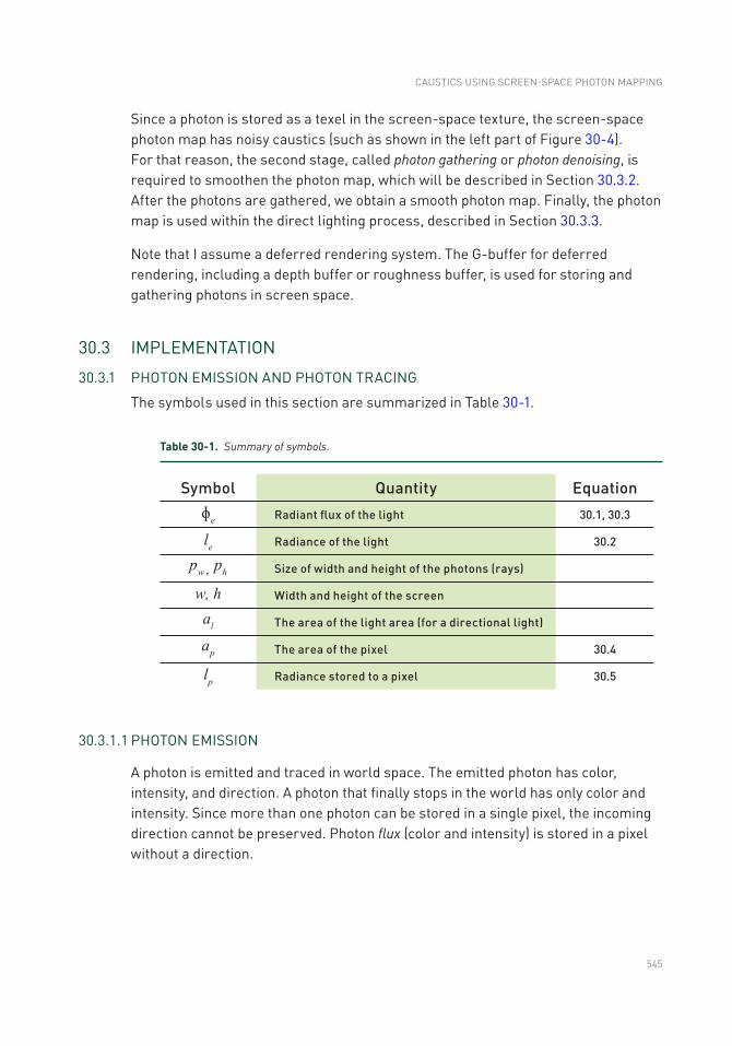
545
Since a photon is stored as a texel in the screen-space texture, the screen-space photon map has noisy caustics (such as shown in the left part of Figure 30-4). For that reason, the second stage, called photon gathering or photon denoising, is required to smoothen the photon map, which will be described in Section 30.3.2. After the photons are gathered, we obtain a smooth photon map. Finally, the photon map is used within the direct lighting process, described in Section 30.3.3.
Note that I assume a deferred rendering system. The G-buffer for deferred rendering, including a depth buffer or roughness buffer, is used for storing and gathering photons in screen space.
30.3 IMPLEMENTATION
30.3.1 PHOTON EMISSION AND PHOTON TRACING
The symbols used in this section are summarized in Table 30-1.
30.3.1.1 PHOTON EMISSION
A photon is emitted and traced in world space. The emitted photon has color, intensity, and direction. A photon that finally stops in the world has only color and intensity. Since more than one photon can be stored in a single pixel, the incoming direction cannot be preserved. Photon flux (color and intensity) is stored in a pixel without a direction.
Table 30-1. Summary of symbols.
CAUSTICS USING SCREEN- SPACE PHOTON MAPPING
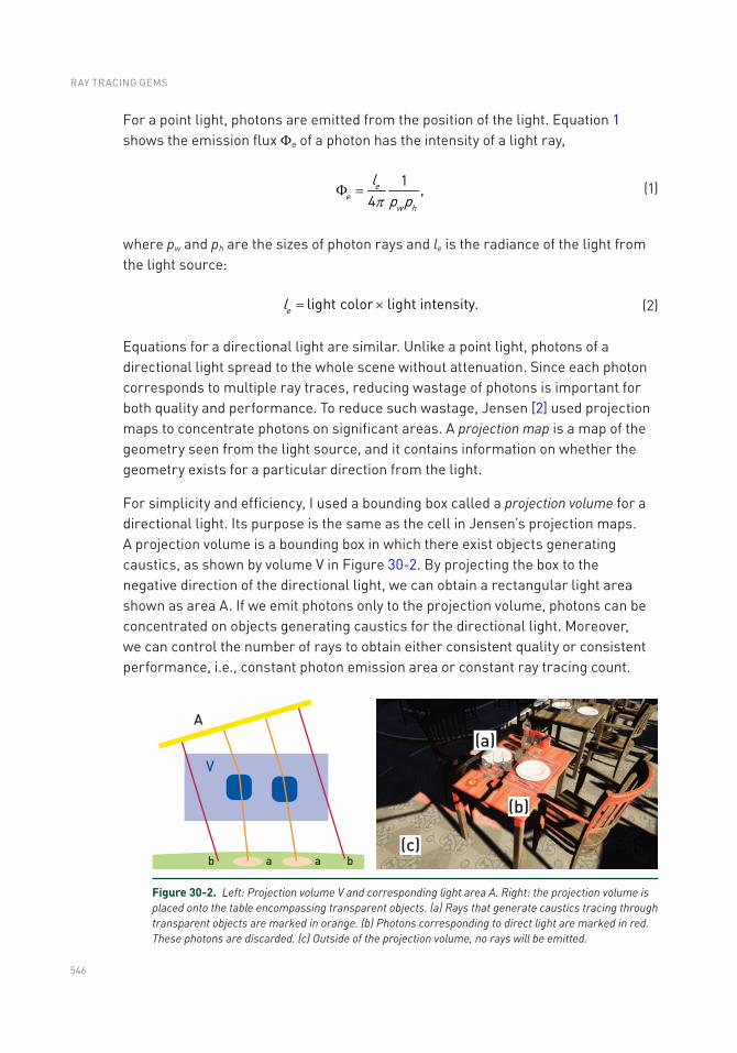
546
For a point light, photons are emitted from the position of the light. Equation 1 shows the emission flux Φe of a photon has the intensity of a light ray,
ee
w h
lp p
1 ,4p
F =
(1)
where pw and ph are the sizes of photon rays and le is the radiance of the light from the light source:
light color light intensity.el = ´ (2)
Equations for a directional light are similar. Unlike a point light, photons of a directional light spread to the whole scene without attenuation. Since each photon corresponds to multiple ray traces, reducing wastage of photons is important for both quality and performance. To reduce such wastage, Jensen [2] used projection maps to concentrate photons on significant areas. A projection map is a map of the geometry seen from the light source, and it contains information on whether the geometry exists for a particular direction from the light.
For simplicity and efficiency, I used a bounding box called a projection volume for a directional light. Its purpose is the same as the cell in Jensen’s projection maps. A projection volume is a bounding box in which there exist objects generating caustics, as shown by volume V in Figure 30-2. By projecting the box to the negative direction of the directional light, we can obtain a rectangular light area shown as area A. If we emit photons only to the projection volume, photons can be concentrated on objects generating caustics for the directional light. Moreover, we can control the number of rays to obtain either consistent quality or consistent performance, i.e., constant photon emission area or constant ray tracing count.
Figure 30-2. Left: Projection volume V and corresponding light area A. Right: the projection volume is placed onto the table encompassing transparent objects. (a) Rays that generate caustics tracing through transparent objects are marked in orange. (b) Photons corresponding to direct light are marked in red. These photons are discarded. (c) Outside of the projection volume, no rays will be emitted.
RAY TRACING GEMS
547
For the resolution of light area A created with projection map V, pwph is the size of the ray generation shader passed to dispatched rays such as a point light. Each ray of the ray generation shader carries a photon emitted from area A. Since each photon corresponds to a portion of the light area, each photon has area 1/(pwph) for light area al. The emission flux of a directional light is
D .le e
w h
al
p pF =
(3)
However, it should be noted that al is the area of light area A in world-space units.
30.3.1.2 PHOTON TRACING
After a photon is emitted, the photon is ray traced in the world until the maximum number of ray tracing steps is reached or a surface hit by the photon is opaque. In more detail, after a ray traces and hits some object, it evaluates material information. If the surface hit by the ray is opaque enough, the photon will stop and the scene depth will be evaluated to check whether the surface would store the photon in screen space or not. If no object is hit, or the photon’s scene depth from the camera is beyond that stored in the depth buffer, the photon will be discarded. Another condition for stopping the photon is when photon intensity is negligibly small, i.e., the photon is diminished while passing through transparent objects.
The red rays in Figure 30-2 correspond to direct light and will not be stored. It is redundant to store a photon from direct lighting since we process direct light in a separate pass. Removing all direct light might create some artifacts around shadow edges in the denoising stages, but these are not very noticeable.
Because tracing a ray through transparent objects is not a special part in photon mapping, I have skipped those details.
In short, there are four conditions under which a photon will not be stored:
1. The photon’s intensity is negligibly small.
2. The location to be stored is out of the screen.
3. The photon travels beyond the stored depth buffer values.
4. The photon is part of direct lighting.
The code for generating photons is in the function rayGenMain of PhotonEmission.rt.hlsl.
CAUSTICS USING SCREEN- SPACE PHOTON MAPPING
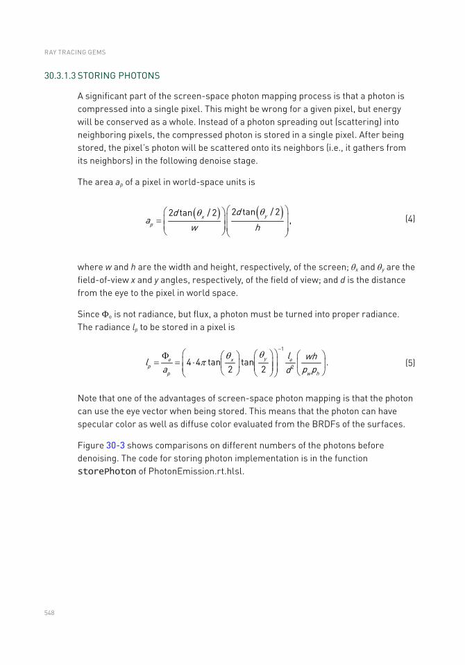
548
30.3.1.3 STORING PHOTONS
A significant part of the screen-space photon mapping process is that a photon is compressed into a single pixel. This might be wrong for a given pixel, but energy will be conserved as a whole. Instead of a photon spreading out (scattering) into neighboring pixels, the compressed photon is stored in a single pixel. After being stored, the pixel’s photon will be scattered onto its neighbors (i.e., it gathers from its neighbors) in the following denoise stage.
The area ap of a pixel in world-space units is
( ) ( )yxp
dda
w h
2 tan / 22 tan / 2,
qq æ öæ öç ÷= ç ÷ç ÷ç ÷è øè ø
(4)
where w and h are the width and height, respectively, of the screen; θx and θy are the field-of-view x and y angles, respectively, of the field of view; and d is the distance from the eye to the pixel in world space.
Since Φe is not radiance, but flux, a photon must be turned into proper radiance. The radiance lp to be stored in a pixel is
ye x ep
p w h
l whla p pd
1
24 4 tan tan .
2 2
qqp
-æ öæ ö æ öF æ ö
= = ç × ÷ç ÷ ç ÷ç ÷ ç ÷ç ÷è ø è øè øè ø (5)
Note that one of the advantages of screen-space photon mapping is that the photon can use the eye vector when being stored. This means that the photon can have specular color as well as diffuse color evaluated from the BRDFs of the surfaces.
Figure 30-3 shows comparisons on different numbers of the photons before denoising. The code for storing photon implementation is in the function storePhoton of PhotonEmission.rt.hlsl.
RAY TRACING GEMS
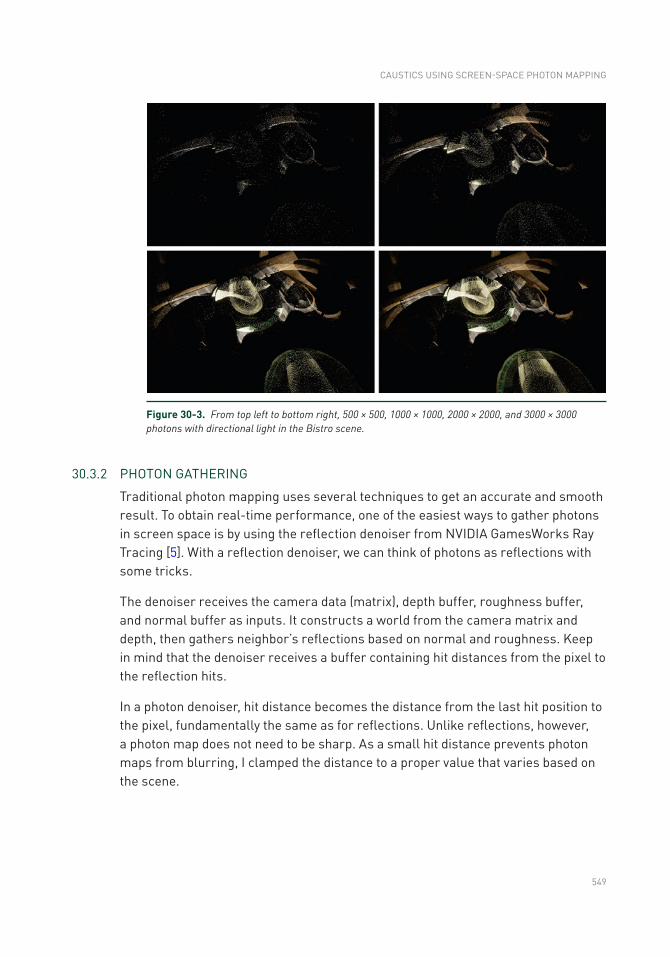
549
30.3.2 PHOTON GATHERING
Traditional photon mapping uses several techniques to get an accurate and smooth result. To obtain real-time performance, one of the easiest ways to gather photons in screen space is by using the reflection denoiser from NVIDIA GamesWorks Ray Tracing [5]. With a reflection denoiser, we can think of photons as reflections with some tricks.
The denoiser receives the camera data (matrix), depth buffer, roughness buffer, and normal buffer as inputs. It constructs a world from the camera matrix and depth, then gathers neighbor’s reflections based on normal and roughness. Keep in mind that the denoiser receives a buffer containing hit distances from the pixel to the reflection hits.
In a photon denoiser, hit distance becomes the distance from the last hit position to the pixel, fundamentally the same as for reflections. Unlike reflections, however, a photon map does not need to be sharp. As a small hit distance prevents photon maps from blurring, I clamped the distance to a proper value that varies based on the scene.
Figure 30-3. From top left to bottom right, 500 × 500, 1000 × 1000, 2000 × 2000, and 3000 × 3000 photons with directional light in the Bistro scene.
CAUSTICS USING SCREEN- SPACE PHOTON MAPPING
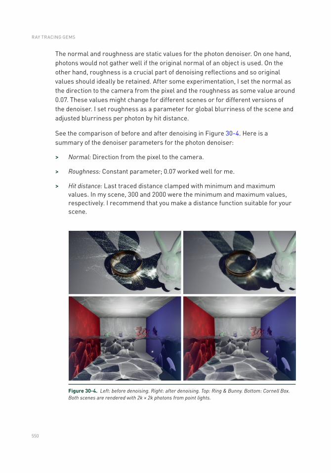
550
The normal and roughness are static values for the photon denoiser. On one hand, photons would not gather well if the original normal of an object is used. On the other hand, roughness is a crucial part of denoising reflections and so original values should ideally be retained. After some experimentation, I set the normal as the direction to the camera from the pixel and the roughness as some value around 0.07. These values might change for different scenes or for different versions of the denoiser. I set roughness as a parameter for global blurriness of the scene and adjusted blurriness per photon by hit distance.
See the comparison of before and after denoising in Figure 30-4. Here is a summary of the denoiser parameters for the photon denoiser:
> Normal: Direction from the pixel to the camera.
> Roughness: Constant parameter; 0.07 worked well for me.
> Hit distance: Last traced distance clamped with minimum and maximum values. In my scene, 300 and 2000 were the minimum and maximum values, respectively. I recommend that you make a distance function suitable for your scene.
Figure 30-4. Left: before denoising. Right: after denoising. Top: Ring & Bunny. Bottom: Cornell Box. Both scenes are rendered with 2k × 2k photons from point lights.
RAY TRACING GEMS
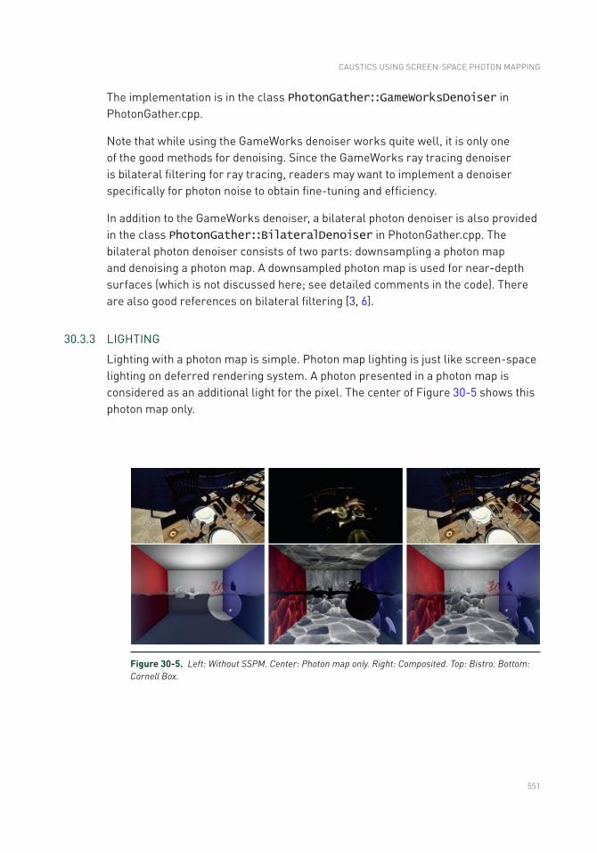
551
The implementation is in the class PhotonGather::GameWorksDenoiser in PhotonGather.cpp.
Note that while using the GameWorks denoiser works quite well, it is only one of the good methods for denoising. Since the GameWorks ray tracing denoiser is bilateral filtering for ray tracing, readers may want to implement a denoiser specifically for photon noise to obtain fine-tuning and efficiency.
In addition to the GameWorks denoiser, a bilateral photon denoiser is also provided in the class PhotonGather::BilateralDenoiser in PhotonGather.cpp. The bilateral photon denoiser consists of two parts: downsampling a photon map and denoising a photon map. A downsampled photon map is used for near-depth surfaces (which is not discussed here; see detailed comments in the code). There are also good references on bilateral filtering [3, 6].
30.3.3 LIGHTING
Lighting with a photon map is simple. Photon map lighting is just like screen-space lighting on deferred rendering system. A photon presented in a photon map is considered as an additional light for the pixel. The center of Figure 30-5 shows this photon map only.
Figure 30-5. Left: Without SSPM. Center: Photon map only. Right: Composited. Top: Bistro. Bottom: Cornell Box.
CAUSTICS USING SCREEN- SPACE PHOTON MAPPING
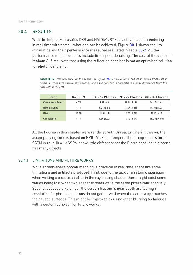
552
30.4 RESULTS
With the help of Microsoft’s DXR and NVIDIA’s RTX, practical caustic rendering in real time with some limitations can be achieved. Figure 30-1 shows results of caustics and their performance measures are listed in Table 30-2. All the performance measurements include time spent denoising. The cost of the denoiser is about 3–5 ms. Note that using the reflection denoiser is not an optimized solution for photon denoising.
Table 30-2. Performance for the scenes in Figure 30-1 on a GeForce RTX 2080 Ti with 1920 × 1080 pixels. All measures are in milliseconds and each number in parentheses is the difference from the cost without SSPM.
All the figures in this chapter were rendered with Unreal Engine 4; however, the accompanying code is based on NVIDIA’s Falcor engine. The timing results for no SSPM versus 1k × 1k SSPM show little difference for the Bistro because this scene has many objects.
30.4.1 LIMITATIONS AND FUTURE WORKS
While screen-space photon mapping is practical in real time, there are some limitations and artifacts produced. First, due to the lack of an atomic operation when writing a pixel to a buffer in the ray tracing shader, there might exist some values being lost when two shader threads write the same pixel simultaneously. Second, because pixels near the screen frustum’s near depth are too high resolution for photons, photons do not gather well when the camera approaches the caustic surfaces. This might be improved by using other blurring techniques with a custom denoiser for future works.
RAY TRACING GEMS
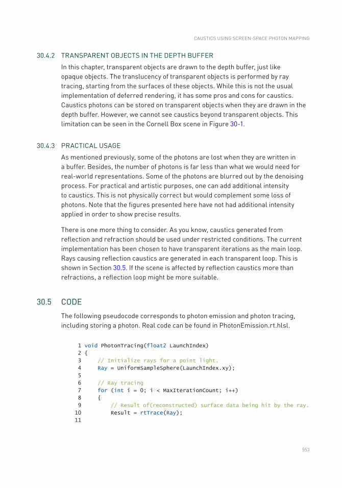
553
30.4.2 TRANSPARENT OBJECTS IN THE DEPTH BUFFER
In this chapter, transparent objects are drawn to the depth buffer, just like opaque objects. The translucency of transparent objects is performed by ray tracing, starting from the surfaces of these objects. While this is not the usual implementation of deferred rendering, it has some pros and cons for caustics. Caustics photons can be stored on transparent objects when they are drawn in the depth buffer. However, we cannot see caustics beyond transparent objects. This limitation can be seen in the Cornell Box scene in Figure 30-1.
30.4.3 PRACTICAL USAGE
As mentioned previously, some of the photons are lost when they are written in a buffer. Besides, the number of photons is far less than what we would need for real-world representations. Some of the photons are blurred out by the denoising process. For practical and artistic purposes, one can add additional intensity to caustics. This is not physically correct but would complement some loss of photons. Note that the figures presented here have not had additional intensity applied in order to show precise results.
There is one more thing to consider. As you know, caustics generated from reflection and refraction should be used under restricted conditions. The current implementation has been chosen to have transparent iterations as the main loop. Rays causing reflection caustics are generated in each transparent loop. This is shown in Section 30.5. If the scene is affected by reflection caustics more than refractions, a reflection loop might be more suitable.
30.5 CODE
The following pseudocode corresponds to photon emission and photon tracing, including storing a photon. Real code can be found in PhotonEmission.rt.hlsl.
1 void PhotonTracing(float2 LaunchIndex)
2
3 // Initialize rays for a point light.
4 Ray = UniformSampleSphere(LaunchIndex.xy);
5
6 // Ray tracing
7 for (int i = 0; i < MaxIterationCount; i++)
8
9 // Result of(reconstructed) surface data being hit by the ray.
10 Result = rtTrace(Ray);
11
CAUSTICS USING SCREEN- SPACE PHOTON MAPPING
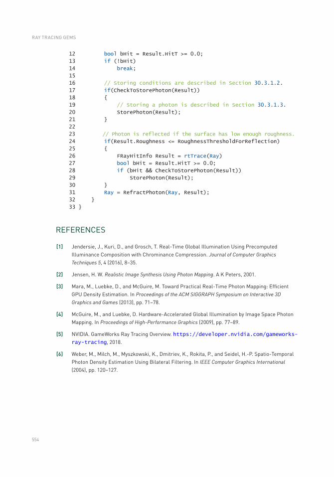
554
12 bool bHit = Result.HitT >= 0.0;
13 if (!bHit)
14 break;
15
16 // Storing conditions are described in Section 30.3.1.2.
17 if(CheckToStorePhoton(Result))
18
19 // Storing a photon is described in Section 30.3.1.3.
20 StorePhoton(Result);
21
22
23 // Photon is reflected if the surface has low enough roughness.
24 if(Result.Roughness <= RoughnessThresholdForReflection)
25
26 FRayHitInfo Result = rtTrace(Ray)
27 bool bHit = Result.HitT >= 0.0;
28 if (bHit && CheckToStorePhoton(Result))
29 StorePhoton(Result);
30
31 Ray = RefractPhoton(Ray, Result);
32
33
REFERENCES
[1] Jendersie, J., Kuri, D., and Grosch, T. Real-Time Global Illumination Using Precomputed Illuminance Composition with Chrominance Compression. Journal of Computer Graphics Techniques 5, 4 (2016), 8–35.
[2] Jensen, H. W. Realistic Image Synthesis Using Photon Mapping. A K Peters, 2001.
[3] Mara, M., Luebke, D., and McGuire, M. Toward Practical Real-Time Photon Mapping: Efficient GPU Density Estimation. In Proceedings of the ACM SIGGRAPH Symposium on Interactive 3D Graphics and Games (2013), pp. 71–78.
[4] McGuire, M., and Luebke, D. Hardware-Accelerated Global Illumination by Image Space Photon Mapping. In Proceedings of High-Performance Graphics (2009), pp. 77–89.
[5] NVIDIA. GameWorks Ray Tracing Overview. https://developer.nvidia.com/gameworks-ray-tracing, 2018.
[6] Weber, M., Milch, M., Myszkowski, K., Dmitriev, K., Rokita, P., and Seidel, H.-P. Spatio-Temporal Photon Density Estimation Using Bilateral Filtering. In IEEE Computer Graphics International (2004), pp. 120–127.
RAY TRACING GEMS

555
Open Access This chapter is licensed under the terms of the Creative Commons Attribution-NonCommercial-NoDerivatives 4.0 International License (http://creativecommons.org/licenses/by-nc-nd/4.0/), which permits any noncommercial use, sharing, distribution and
reproduction in any medium or format, as long as you give appropriate credit to the original author(s) and the source, provide a link to the Creative Commons license and indicate if you modified the licensed material. You do not have permission under this license to share adapted material derived from this chapter or parts of it.
The images or other third party material in this chapter are included in the chapter's Creative Commons license, unless indicated otherwise in a credit line to the material. If material is not included in the chapter's Creative Commons license and your intended use is not permitted by statutory regulation or exceeds the permitted use, you will need to obtain permission directly from the copyright holder.
CAUSTICS USING SCREEN- SPACE PHOTON MAPPING
557© NVIDIA 2019 E. Haines, T. Akenine-Möller (eds.), Ray Tracing Gems, https://doi.org/10.1007/978-1-4842-4427-2_31
CHAPTER 31
Variance Reduction via Footprint Estimation in the Presence of Path ReuseJohannes JendersieClausthal University of Technology
ABSTRACT
Multiple importance sampling is a tool to weight the results of different samplers with the goal of a minimal variance for the sampled function. If applied to light transport paths, this tool enables techniques such as bidirectional path tracing and vertex connection and merging. The latter generalizes the path probability measure to merges—also known as photon mapping. Unfortunately, the resulting heuristic can fail, resulting in a noticeable increase of noise. This chapter provides an insight into why things go wrong and proposes a simple-to-implement heuristic that is closer to an optimal solution and more reliable over different scenes. The trick is to use footprint estimates of sub-paths to predict the true variance reduction that is introduced by reusing all the photons.
31.1 INTRODUCTION
In light transport simulation there is a multitude of sampling strategies, visualized in Figure 31-1. By tracing paths, beginning at a sensor, we can randomly find light sources in the scene and compute their contributions through the sampled paths. Additionally, next event estimation, the connection toward a known light source, helps to locate smaller light sources. Both sampling strategies together form the path tracing (PT) algorithm, introduced by Kajiya [8]. In bidirectional path tracing (BPT) [9, 13] all possible connections between a random view sub-path and a random light sub-path provide additional samplers. BPT is able to find caustic paths using the camera connection, something not possible in PT.
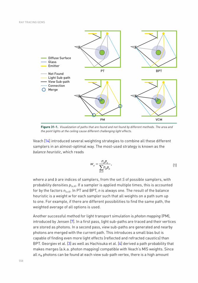
558
Veach [14] introduced several weighting strategies to combine all these different samplers in an almost-optimal way. The most-used strategy is known as the balance heuristic, which reads
a aa
b bb S
n pw
n p,
Î
=å
(1)
where a and b are indices of samplers, from the set S of possible samplers, with probability densities pa, b. If a sampler is applied multiple times, this is accounted for by the factors na, b. In PT and BPT, n is always one. The result of the balance heuristic is a weight w for each sampler such that all weights on a path sum up to one. For example, if there are different possibilities to find the same path, the weighted average of all options is used.
Another successful method for light transport simulation is photon mapping (PM), introduced by Jensen [7]. In a first pass, light sub-paths are traced and their vertices are stored as photons. In a second pass, view sub-paths are generated and nearby photons are merged with the current path. This introduces a small bias but is capable of finding even more light effects (reflected and refracted caustics) than BPT. Georgiev et al. [3] as well as Hachisuka et al. [4] derived a path probability that makes merges (a.k.a. photon mapping) compatible with Veach’s MIS weights. Since all nΦ photons can be found at each view sub-path vertex, there is a high amount
Figure 31-1. Visualization of paths that are found and not found by different methods. The area and the point lights at the ceiling cause different challenging light effects.
RAY TRACING GEMS
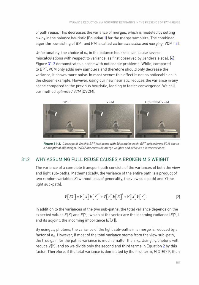
559
of path reuse. This decreases the variance of merges, which is modeled by setting n = nΦ in the balance heuristic (Equation 1) for the merge samplers. The combined algorithm consisting of BPT and PM is called vertex connection and merging (VCM) [3].
Unfortunately, the choice of nΦ in the balance heuristic can cause severe miscalculations with respect to variance, as first observed by Jendersie et al. [6]. Figure 31-2 demonstrates a scene with noticeable problems. While, compared to BPT, VCM only adds new samplers and therefore should only decrease the variance, it shows more noise. In most scenes this effect is not as noticeable as in the chosen example. However, using our new heuristic reduces the variance in any scene compared to the previous heuristic, leading to faster convergence. We call our method optimized VCM (OVCM).
Figure 31-2. Closeups of Veach’s BPT test scene with 50 samples each. BPT outperforms VCM due to a nonoptimal MIS weight. OVCM improves the merge weights and achieves a lower variance.
31.2 WHY ASSUMING FULL REUSE CAUSES A BROKEN MIS WEIGHT
The variance of a complete transport path consists of the variances of both the view and light sub-paths. Mathematically, the variance of the entire path is a product of two random variables X (without loss of generality, the view sub-path) and Y (the light sub- path):
V XY V X E Y V Y E X V X V Y
2 2.é ù = é ù é ù + é ù é ù + é ù é ùë û ë û ë û ë û ë û ë û ë û (2)
In addition to the variances of the two sub-paths, the total variance depends on the expected values E[ X ] and E[Y ], which at the vertex are the incoming radiance (E[Y ]) and its adjoint, the incoming importance (E[ X ]).
By using nΦ photons, the variance of the light sub-paths in a merge is reduced by a factor of nΦ. However, if most of the total variance stems from the view sub-path, the true gain for the path’s variance is much smaller than nΦ. Using nΦ photons will reduce V[Y ], and so we divide only the second and third terms in Equation 2 by this factor. Therefore, if the total variance is dominated by the first term, V[ X ]E[Y ]2, then
VARIANCE REDUCTION VIA FOOTPRINT ESTIMATION IN THE PRESENCE OF PATH REUSE
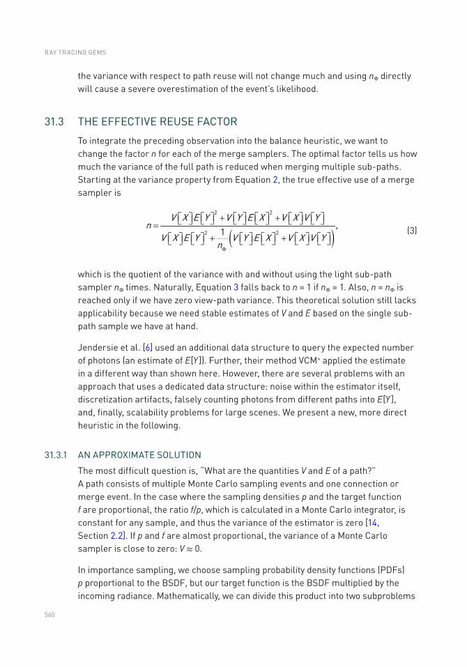
560
the variance with respect to path reuse will not change much and using nΦ directly will cause a severe overestimation of the event’s likelihood.
31.3 THE EFFECTIVE REUSE FACTOR
To integrate the preceding observation into the balance heuristic, we want to change the factor n for each of the merge samplers. The optimal factor tells us how much the variance of the full path is reduced when merging multiple sub-paths. Starting at the variance property from Equation 2, the true effective use of a merge sampler is
( )V X E Y V Y E X V X V Y
nV X E Y V Y E X V X V Y
n
2 2
2 2,
1
F
é ù é ù + é ù é ù + é ù é ùë û ë û ë û ë û ë û ë û=é ù é ù + é ù é ù + é ù é ùë û ë û ë û ë û ë û ë û
(3)
which is the quotient of the variance with and without using the light sub-path sampler nΦ times. Naturally, Equation 3 falls back to n = 1 if nΦ = 1. Also, n = nΦ is reached only if we have zero view-path variance. This theoretical solution still lacks applicability because we need stable estimates of V and E based on the single sub-path sample we have at hand.
Jendersie et al. [6] used an additional data structure to query the expected number of photons (an estimate of E[Y ]). Further, their method VCM∗ applied the estimate in a different way than shown here. However, there are several problems with an approach that uses a dedicated data structure: noise within the estimator itself, discretization artifacts, falsely counting photons from different paths into E[Y ], and, finally, scalability problems for large scenes. We present a new, more direct heuristic in the following.
31.3.1 AN APPROXIMATE SOLUTION
The most difficult question is, “What are the quantities V and E of a path?” A path consists of multiple Monte Carlo sampling events and one connection or merge event. In the case where the sampling densities p and the target function f are proportional, the ratio f/p, which is calculated in a Monte Carlo integrator, is constant for any sample, and thus the variance of the estimator is zero [14, Section 2.2]. If p and f are almost proportional, the variance of a Monte Carlo sampler is close to zero: V ≈ 0.
In importance sampling, we choose sampling probability density functions (PDFs) p proportional to the BSDF, but our target function is the BSDF multiplied by the incoming radiance. Mathematically, we can divide this product into two subproblems
RAY TRACING GEMS
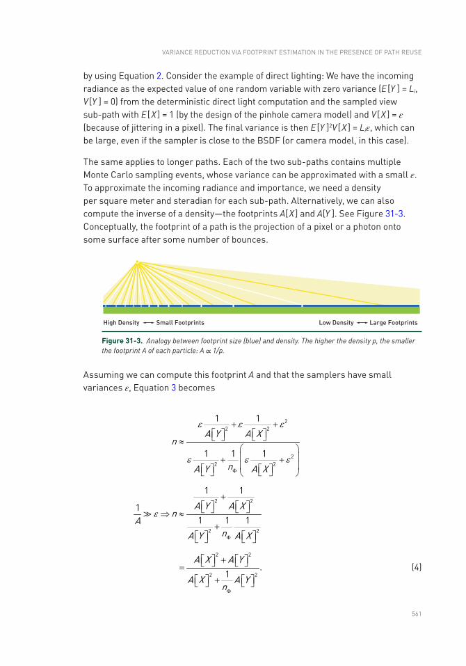
561
by using Equation 2. Consider the example of direct lighting: We have the incoming radiance as the expected value of one random variable with zero variance (E [Y ] = Li, V [Y ] = 0) from the deterministic direct light computation and the sampled view sub-path with E [ X ] = 1 (by the design of the pinhole camera model) and V [ X ] = ε (because of jittering in a pixel). The final variance is then E [Y ]2V [ X ] = Liε, which can be large, even if the sampler is close to the BSDF (or camera model, in this case).
The same applies to longer paths. Each of the two sub-paths contains multiple Monte Carlo sampling events, whose variance can be approximated with a small ε. To approximate the incoming radiance and importance, we need a density per square meter and steradian for each sub-path. Alternatively, we can also compute the inverse of a density—the footprints A[ X ] and A[Y ]. See Figure 31-3. Conceptually, the footprint of a path is the projection of a pixel or a photon onto some surface after some number of bounces.
Figure 31-3. Analogy between footprint size (blue) and density. The higher the density p, the smaller the footprint A of each particle: A ∝ 1/p.
Assuming we can compute this footprint A and that the samplers have small variances ε, Equation 3 becomes
A Y A Xn
nA Y A X
22 2
22 2
1 1
1 1 1
e e e
e e eF
+ +é ù é ùë û ë û»
æ öç ÷+ +ç ÷é ù é ùë û ë ûè ø
A Y A Xn
AnA Y A X
2 2
2 2
1 1
11 1 1
e
F
+é ù é ùë û ë ûÞ »
+é ù é ùë û ë û
A X A Y
A X A Yn
2 2
2 2.
1
F
é ù + é ùë û ë û=é ù + é ùë û ë û
(4)
VARIANCE REDUCTION VIA FOOTPRINT ESTIMATION IN THE PRESENCE OF PATH REUSE
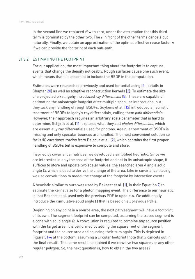
562
In the second line we replaced ε2 with zero, under the assumption that this third term is dominated by the other two. The ε in front of the other terms cancels out naturally. Finally, we obtain an approximation of the optimal effective reuse factor n if we can provide the footprint of each sub-path.
31.3.2 ESTIMATING THE FOOTPRINT
For our application, the most important thing about the footprint is to capture events that change the density noticeably. Rough surfaces cause one such event, which means that it is essential to include the BSDF in the computation.
Estimates were researched previously and used for antialiasing [5] (details in Chapter 20) as well as adaptive reconstruction kernels [2]. To estimate the size of a projected pixel, Igehy introduced ray differentials [5]. These are capable of estimating the anisotropic footprint after multiple specular interactions, but they lack any handling of rough BSDFs. Suykens et al. [12] introduced a heuristic treatment of BSDFs to Igehy’s ray differentials, calling them path differentials. However, their approach requires an arbitrary scale parameter that is hard to determine. Schjøth et al. [11] explored what they call photon differentials, which are essentially ray differentials used for photons. Again, a treatment of BSDFs is missing and only specular bounces are handled. The most convenient solution so far is 5D covariance tracing from Belcour et al. [2], which contains the first proper handling of BSDFs but is expensive to compute and store.
Inspired by covariance matrices, we developed a simplified heuristic. Since we are interested in only the area of the footprint and not in its anisotropic shape, it suffices to store and update two scalar values: the searched area A and a solid angle Ω, which is used to derive the change of the area. Like in covariance tracing, we use convolutions to model the change of the footprint by interaction events.
A heuristic similar to ours was used by Bekaert et al. [1], in their Equation 7, to estimate the kernel size for a photon mapping event. The difference to our heuristic is that Bekeart et al. used only the previous PDF to update A. We additionally introduce the cumulative solid angle Ω that is based on all previous PDFs.
Beginning on any point in a source area, the next path segment will have a footprint of its own. The segment footprint can be computed, assuming the traced segment is a cone with solid angle Ω. A convolution is required to combine any source position with the target area. It is performed by adding the square root of the segment footprint and the source area and squaring their sum again. This is depicted in Figure 31-4 at the bottom, assuming a circular footprint (note that π cancels out in the final result). The same result is obtained if we convolve two squares or any other regular polygon. So, the next question is, how to obtain the two areas?
RAY TRACING GEMS
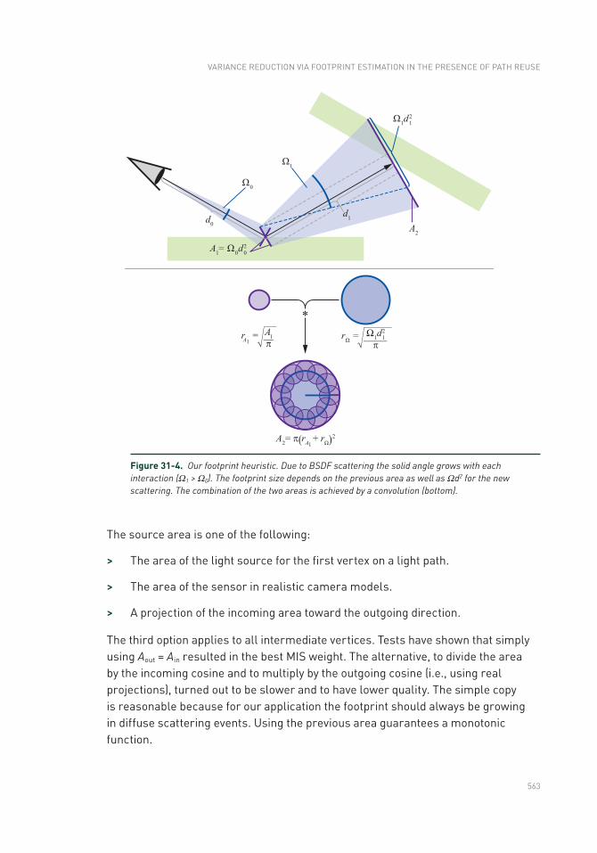
563
Figure 31-4. Our footprint heuristic. Due to BSDF scattering the solid angle grows with each interaction (Ω1 > Ω0). The footprint size depends on the previous area as well as Ωd2 for the new scattering. The combination of the two areas is achieved by a convolution (bottom).
The source area is one of the following:
> The area of the light source for the first vertex on a light path.
> The area of the sensor in realistic camera models.
> A projection of the incoming area toward the outgoing direction.
The third option applies to all intermediate vertices. Tests have shown that simply using Aout = Ain resulted in the best MIS weight. The alternative, to divide the area by the incoming cosine and to multiply by the outgoing cosine (i.e., using real projections), turned out to be slower and to have lower quality. The simple copy is reasonable because for our application the footprint should always be growing in diffuse scattering events. Using the previous area guarantees a monotonic function.
VARIANCE REDUCTION VIA FOOTPRINT ESTIMATION IN THE PRESENCE OF PATH REUSE
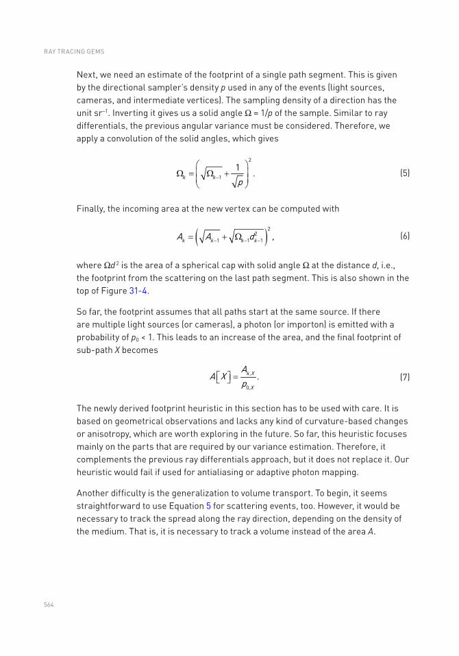
564
Next, we need an estimate of the footprint of a single path segment. This is given by the directional sampler’s density p used in any of the events (light sources, cameras, and intermediate vertices). The sampling density of a direction has the unit sr−1. Inverting it gives us a solid angle Ω = 1/p of the sample. Similar to ray differentials, the previous angular variance must be considered. Therefore, we apply a convolution of the solid angles, which gives
k k p
2
1
1 .-
æ öç ÷W = W +ç ÷è ø
(5)
Finally, the incoming area at the new vertex can be computed with
( )k k k kA A d
22
1 1 1 ,- - -= + W
(6)
where Ωd 2 is the area of a spherical cap with solid angle Ω at the distance d, i.e., the footprint from the scattering on the last path segment. This is also shown in the top of Figure 31-4.
So far, the footprint assumes that all paths start at the same source. If there are multiple light sources (or cameras), a photon (or importon) is emitted with a probability of p0 < 1. This leads to an increase of the area, and the final footprint of sub-path X becomes
k X
X
AA X
p,
0,
.é ù =ë û
(7)
The newly derived footprint heuristic in this section has to be used with care. It is based on geometrical observations and lacks any kind of curvature-based changes or anisotropy, which are worth exploring in the future. So far, this heuristic focuses mainly on the parts that are required by our variance estimation. Therefore, it complements the previous ray differentials approach, but it does not replace it. Our heuristic would fail if used for antialiasing or adaptive photon mapping.
Another difficulty is the generalization to volume transport. To begin, it seems straightforward to use Equation 5 for scattering events, too. However, it would be necessary to track the spread along the ray direction, depending on the density of the medium. That is, it is necessary to track a volume instead of the area A.
RAY TRACING GEMS
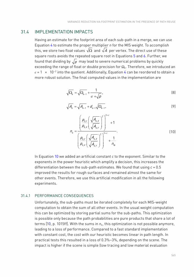
565
31.4 IMPLEMENTATION IMPACTS
Having an estimate for the footprint area of each sub-path in a merge, we can use Equation 4 to estimate the proper multiplier n for the MIS weight. To accomplish this, we store two float values W and A per vertex. The direct use of these square roots avoids the repeated square root in Equations 5 and 6. Further, we found that dividing by p may lead to severe numerical problems by quickly exceeding the range of float or double precision for Ωk. Therefore, we introduced an ϵ = 1 × 10⁻² into the quotient. Additionally, Equation 4 can be reordered to obtain a more robust solution. The final computed values in the implementation are
k k p1
1 ,Î
-W = W ++
(8)
k k k kA A d1 1 1,- - -= + W (9)
c
k XY
X k Y
k c
k XY
X k Y
App A
nAp
p nA
22
,0,
0, ,
22
,0,
0, ,
1
.
1
+
+
F
æ öæ öç ÷ç ÷ +ç ÷ç ÷ç ÷è øè ø=æ öæ öç ÷ç ÷ +ç ÷ç ÷ç ÷è øè ø
(10)
In Equation 10 we added an artificial constant c to the exponent. Similar to the exponents in the power heuristic which amplify a decision, this increases the differentiation between the sub-path estimates. We found that using c = 0.5 improved the results for rough surfaces and remained almost the same for other events. Therefore, we use this artificial modification in all the following experiments.
31.4.1 PERFORMANCE CONSEQUENCES
Unfortunately, the sub-paths must be iterated completely for each MIS-weight computation to obtain the sum of all other events. In the usual weight computation this can be optimized by storing partial sums for the sub-paths. This optimization is possible only because the path probabilities are pure products that share a lot of terms [10, p. 1015ff]. With the sums in nk, this optimization is not possible anymore, leading to a loss of performance. Compared to a fast standard implementation with constant cost, the cost with our heuristic becomes linear in path length. In practical tests this resulted in a loss of 0.3%–3%, depending on the scene. The impact is higher if the scene is simple (low tracing and low material evaluation
VARIANCE REDUCTION VIA FOOTPRINT ESTIMATION IN THE PRESENCE OF PATH REUSE
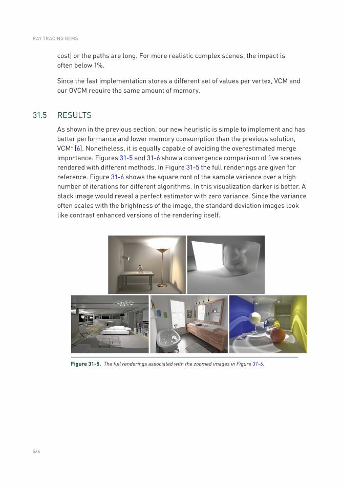
566
cost) or the paths are long. For more realistic complex scenes, the impact is often below 1%.
Since the fast implementation stores a different set of values per vertex, VCM and our OVCM require the same amount of memory.
31.5 RESULTS
As shown in the previous section, our new heuristic is simple to implement and has better performance and lower memory consumption than the previous solution, VCM∗ [6]. Nonetheless, it is equally capable of avoiding the overestimated merge importance. Figures 31-5 and 31-6 show a convergence comparison of five scenes rendered with different methods. In Figure 31-5 the full renderings are given for reference. Figure 31- 6 shows the square root of the sample variance over a high number of iterations for different algorithms. In this visualization darker is better. A black image would reveal a perfect estimator with zero variance. Since the variance often scales with the brightness of the image, the standard deviation images look like contrast enhanced versions of the rendering itself.
Figure 31-5. The full renderings associated with the zoomed images in Figure 31-6.
RAY TRACING GEMS
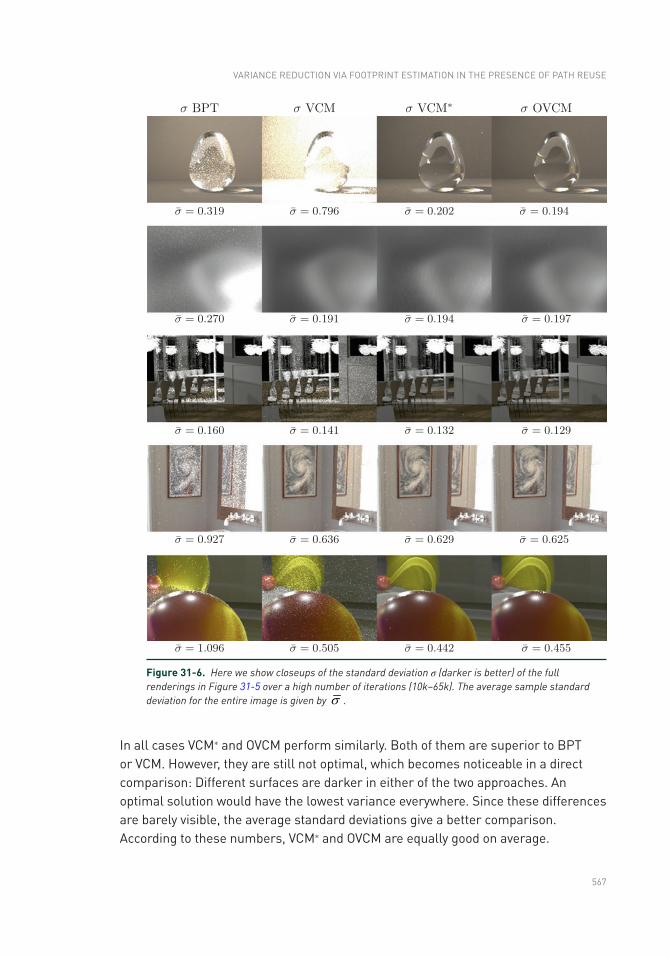
567
In all cases VCM∗ and OVCM perform similarly. Both of them are superior to BPT or VCM. However, they are still not optimal, which becomes noticeable in a direct comparison: Different surfaces are darker in either of the two approaches. An optimal solution would have the lowest variance everywhere. Since these differences are barely visible, the average standard deviations give a better comparison. According to these numbers, VCM∗ and OVCM are equally good on average.
Figure 31-6. Here we show closeups of the standard deviation σ (darker is better) of the full renderings in Figure 31-5 over a high number of iterations (10k–65k). The average sample standard deviation for the entire image is given by s .
VARIANCE REDUCTION VIA FOOTPRINT ESTIMATION IN THE PRESENCE OF PATH REUSE
568
There is also room for improvement. Equation 3 formulates the optimal solution. Our proposed heuristic completely removes all variances V and approximates the expected values E with another heuristic, which, for example, neglects the curvature or texture changes in the footprint area. By improving the estimates of V and E, we expect that the artificial c = 0.5 from Equation 10 will become redundant and that the heuristic will be closer to the optimum.
ACKNOWLEDGMENTS
Most scenes shown here are taken from the repository of Physically Based Rendering (third edition) [10]. The colorful balls scene is courtesy of T. Hachisuka.
REFERENCES
[1] Bekaert, P., Slusallek, P., Cools, R., Havran, V., and Seidel, H.-P. A Custom Designed Density Estimator for Light Transport. Research Report MPI-I-2003-4-004, Max- Planck Institut für Informatik, 2003.
[2] Belcour, L., Soler, C., Subr, K., Holzschuch, N., and Durand, F. 5D Covariance Tracing for Efficient Defocus and Motion Blur. ACM Transaction on Graphics 32, 3 (July 2013), 31:1–31:18.
[3] Georgiev, I., Křivánek, J., Davidovič, T., and Slusallek, P. Light Transport Simulation with Vertex Connection and Merging. ACM Transactions on Graphics (SIGGRAPH Asia) 31, 6 (2012), 192:1–192:10.
[4] Hachisuka, T., Pantaleoni, J., and Jensen, H. W. A Path Space Extension for Robust Light Transport Simulation. ACM Transactions on Graphics (SIGGRAPH Asia) 31, 6 (Nov. 2012), 191:1–191:10.
[5] Igehy, H. Tracing Ray Differentials. In Proceedings of SIGGRAPH (1999), pp. 179–186.
[6] Jendersie, J., and Grosch, T. An Improved Multiple Importance Sampling Heuristic for Density Estimates in Light Transport Simulations. In Eurographics Symposium on Rendering EI&I Track (July 2018), pp. 65–72.
[7] Jensen, H. W. Global Illumination Using Photon Maps. In Eurographics Workshop on Rendering (1996), pp. 21–30.
[8] Kajiya, J. T. The Rendering Equation. Computer Graphics (SIGGRAPH) (1986), 143–150.
[9] Lafortune, E. P., and Willems, Y. D. Bi-Directional Path Tracing. In Conference on Computational Graphics and Visualization Techniques (1993), pp. 145–153.
[10] Pharr, M., Jakob, W., and Humphreys, G. Physically Based Rendering: From Theory to Implementation, third ed. Morgan Kaufmann, 2016.
RAY TRACING GEMS
569
[11] Schjøth, L., Frisvad, J. R., Erleben, K., and Sporring, J. Photon Differentials. In Computer Graphics and Interactive Techniques (Dec. 2007), pp. 179–186.
[12] Suykens, F., and Willems, Y. D. Path Differentials and Applications. In Eurographics Workshop on Rendering (June 2001), pp. 257–268.
[13] Veach, E., and Guibas, L. J. Bidirectional Estimators for Light Transport. In Photorealistic Rendering Techniques. Springer, 1995, pp. 145–167.
[14] Veach, E., and Guibas, L. J. Optimally Combining Sampling Techniques for Monte Carlo Rendering. In Proceedings of SIGGRAPH (1995), pp. 419–428.
Open Access This chapter is licensed under the terms of the Creative Commons Attribution-NonCommercial-NoDerivatives 4.0 International License (http://creativecommons.org/licenses/by-nc-nd/4.0/), which permits any noncommercial use, sharing, distribution and
reproduction in any medium or format, as long as you give appropriate credit to the original author(s) and the source, provide a link to the Creative Commons license and indicate if you modified the licensed material. You do not have permission under this license to share adapted material derived from this chapter or parts of it.
The images or other third party material in this chapter are included in the chapter's Creative Commons license, unless indicated otherwise in a credit line to the material. If material is not included in the chapter's Creative Commons license and your intended use is not permitted by statutory regulation or exceeds the permitted use, you will need to obtain permission directly from the copyright holder.
VARIANCE REDUCTION VIA FOOTPRINT ESTIMATION IN THE PRESENCE OF PATH REUSE
571© NVIDIA 2019 E. Haines, T. Akenine-Möller (eds.), Ray Tracing Gems, https://doi.org/10.1007/978-1-4842-4427-2_32
CHAPTER 32
Accurate Real-Time Specular Reflections with Radiance CachingAntti Hirvonen, Atte Seppälä, Maksim Aizenshtein, and Niklas Smal
UL Benchmarks
ABSTRACT
We present an algorithm for perspective-correct, real-time specular illumination for surfaces of varying glossiness in dynamic environments. Our algorithm leverages properties from earlier techniques (e.g., radiance probes and screen-space reflections) while reducing the amount of visual errors by adding ray tracing to the rendering pipeline. Our algorithm extends previous work by allowing accurate reflections for all surfaces regardless of the material, and it has global coherence (i.e., there are no visible discontinuities). With radiance caching, multiple samples can be efficiently computed as the radiance computation is decoupled from the final shading. The radiance cache is also used to approximate the specular term for the roughest surfaces without any ray tracing.
32.1 INTRODUCTION
Real-time rendering engines approximate lighting computations due to the computational cost of accurate simulations. Lighting can be quickly evaluated only for idealized or nearly idealized light sources such as point lights. However, illumination is a global phenomena and it can be affected significantly by light reflected from surfaces and light emitted from complex sources. Simulation of these components is usually expensive, but both have to be taken into account for realistic lighting. The aggregated contribution of such terms is known as global illumination. In real-time graphics, most terms of global illumination are usually precomputed.
Rendering engines commonly split the surface into two separate layers that contribute to the illumination: diffuse and specular. Each layer is composed of microscopic, flat area elements called microfacets which are described by a distribution rather than geometrical modeling. The mean slope (or in some cases the standard deviation of the slope) is described by a surface parameter called roughness.
572
Diffuse layers describe weak correlation between the scattering distribution and the incoming light direction. A diffuse microfacet scatters luminous energy proportionally to the cosine of the angle between the incoming light direction and the microfacet normal direction. A diffuse material that exhibits flat micro-structure is called Lambertian. In the case of diffuse illumination, the response mostly depends on the total irradiance on the surface. Therefore, the actual distribution of the incoming light does not have to be known in order to compute the radiance scattered in some direction. This observation is the key idea behind precomputed irradiance caches such as light maps or irradiance probes. Due to the low-frequency nature of the input data, the irradiance component can be packed aggressively and stored efficiently to cover the entire scene. Furthermore, minor changes in the scene’s direct diffuse illumination do not significantly affect the indirect diffuse term.
The second term, specular illumination, describes strong correlation between the scattering distribution and the light’s incoming direction. Every specular microfacet reflects light according to Snell’s law, and the reflected energy of the light is determined by Fresnel equations. A surface that exhibits flat micro-structure with specular microfacets is an idealized mirror. However, materials are rarely perfect mirrors and they scatter light into some preferred set of directions instead of just one: such surfaces are classified as glossy specular. By Helmholtz reciprocity, the measured radiance depends on a set of incoming radiances, taking a wider distribution into account when materials are rougher. The specular term is also referred to as reflection later in this chapter.
These observations make it impractical to store many radiance samples regardless of the data structure. Therefore, current rendering engines usually just capture radiance from a few points in the scene, or use already computed main camera radiance for the specular environment term. These approximations have their own shortcomings, which are analyzed briefly in Section 32.2. The only practical way to compute an accurate specular term during runtime is to actually sample radiance from the scene for each shaded point.
In this chapter, we present an algorithm for efficient computation of the indirect specular term for surfaces of varying glossiness regardless of the scene. We use the new Microsoft DirectX Raytracing (DXR) pipeline, as introduced into DirectX 12, to query global surface visibility in the scene for a set of rays defined by the specular BRDF. Radiance for these rays can be efficiently computed with our cached approach. Our algorithm also enables efficient specular term approximation for rough surfaces for which the view-dependent variance is low. The end result after post-filtering provides accurate and real-time specular illumination estimates for each pixel on the screen. See Figure 32-1.
RAY TRACING GEMS
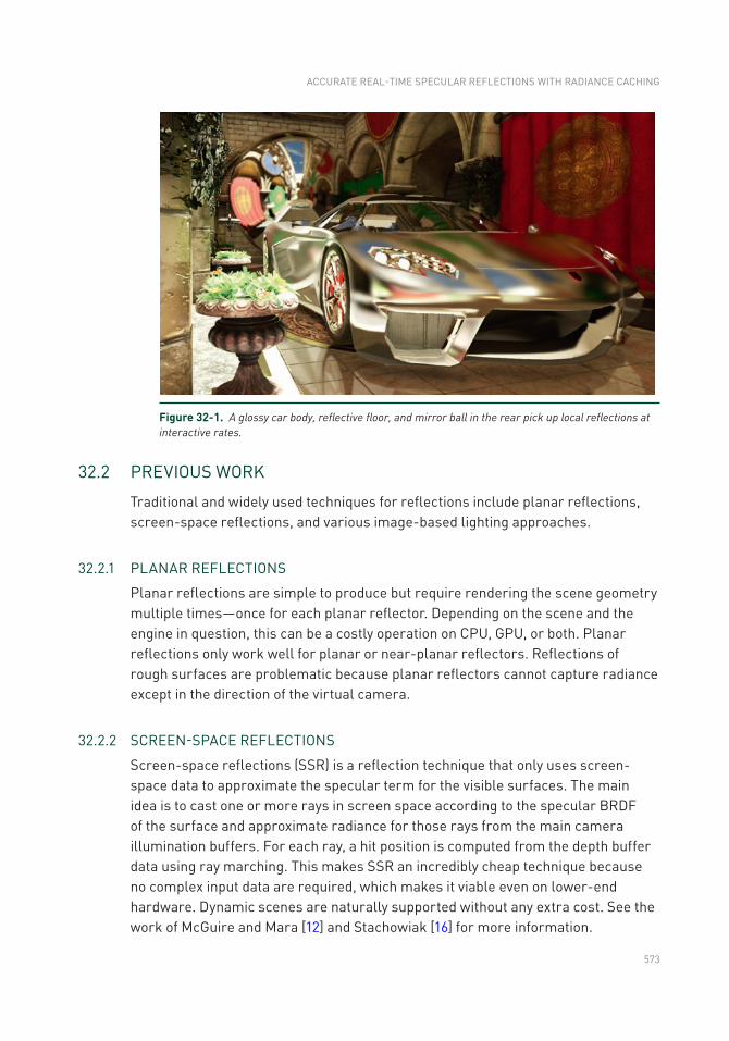
573
32.2 PREVIOUS WORK
Traditional and widely used techniques for reflections include planar reflections, screen- space reflections, and various image-based lighting approaches.
32.2.1 PLANAR REFLECTIONS
Planar reflections are simple to produce but require rendering the scene geometry multiple times—once for each planar reflector. Depending on the scene and the engine in question, this can be a costly operation on CPU, GPU, or both. Planar reflections only work well for planar or near-planar reflectors. Reflections of rough surfaces are problematic because planar reflectors cannot capture radiance except in the direction of the virtual camera.
32.2.2 SCREEN-SPACE REFLECTIONS
Screen-space reflections (SSR) is a reflection technique that only uses screen-space data to approximate the specular term for the visible surfaces. The main idea is to cast one or more rays in screen space according to the specular BRDF of the surface and approximate radiance for those rays from the main camera illumination buffers. For each ray, a hit position is computed from the depth buffer data using ray marching. This makes SSR an incredibly cheap technique because no complex input data are required, which makes it viable even on lower-end hardware. Dynamic scenes are naturally supported without any extra cost. See the work of McGuire and Mara [12] and Stachowiak [16] for more information.
Figure 32-1. A glossy car body, reflective floor, and mirror ball in the rear pick up local reflections at interactive rates.
ACCURATE REAL-TIME SPECULAR REFLECTIONS WITH RADIANCE CACHING
574
Unfortunately, SSR has multiple downsides. First, as it only operates on the screen- space data, occlusion can be incorrectly interpreted based on the depth buffer. In such cases, a ray can either terminate too early or pass through objects that it should actually hit. Second, main camera radiance naturally has only a single layer, and thus objects occluded in the view of main camera or outside of the camera frustum are not seen in reflections.
32.2.3 IMAGE-BASED LIGHTING
Image-based lighting (IBL) techniques approximate illumination from some captured imagery, stored usually in radiance probes that encode a spherical radiance map (also known as radiance cubes, reflection cubes, or reflection probes). Each probe can be associated with a proxy geometry object, such as a sphere or a box, that gives an approximated hit point in the scene [11]. Probes are also usually prefiltered to allow fast approximation of glossy materials and can be either precomputed or updated in real time depending on the frame budget. Readers can refer to Debevec’s work [3] for more information on IBL in general.
32.2.4 HYBRID APPROACHES
Multiple reflection techniques are usually combined to produce the final image. For example, screen-space reflections can be used in conjunction with the offline-generated radiance probes to create an approximate real-time specular illumination [5]. However, mixing various techniques can lead to visible discontinuities in the final illumination at the places where the reflection technique switches.
32.2.5 MISCELLANEOUS
More recent approaches have higher quality, but they come with an added computational cost. Voxel cone tracing can produce realistic specular terms even in dynamic scenes as presented by Crassin et al. [1], but it operates on the voxel scale. The approach presented by McGuire et al. [13] allows computation of accurate indirect diffuse and specular illumination from a set of precomputed light probes. These probes are augmented with a depth buffer for computing the intersection with a similar ray marching routine as in screen-space reflections. However, the technique is not fully dynamic. Neither of these techniques are yet widely used in rendering engines.
RAY TRACING GEMS
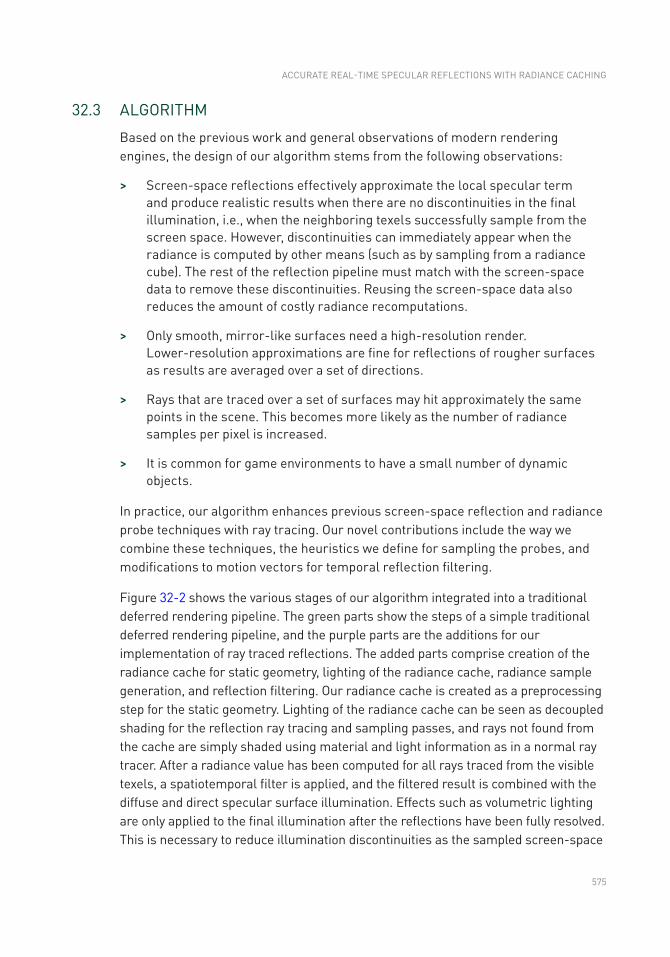
575
32.3 ALGORITHM
Based on the previous work and general observations of modern rendering engines, the design of our algorithm stems from the following observations:
> Screen-space reflections effectively approximate the local specular term and produce realistic results when there are no discontinuities in the final illumination, i.e., when the neighboring texels successfully sample from the screen space. However, discontinuities can immediately appear when the radiance is computed by other means (such as by sampling from a radiance cube). The rest of the reflection pipeline must match with the screen-space data to remove these discontinuities. Reusing the screen-space data also reduces the amount of costly radiance recomputations.
> Only smooth, mirror-like surfaces need a high-resolution render. Lower-resolution approximations are fine for reflections of rougher surfaces as results are averaged over a set of directions.
> Rays that are traced over a set of surfaces may hit approximately the same points in the scene. This becomes more likely as the number of radiance samples per pixel is increased.
> It is common for game environments to have a small number of dynamic objects.
In practice, our algorithm enhances previous screen-space reflection and radiance probe techniques with ray tracing. Our novel contributions include the way we combine these techniques, the heuristics we define for sampling the probes, and modifications to motion vectors for temporal reflection filtering.
Figure 32-2 shows the various stages of our algorithm integrated into a traditional deferred rendering pipeline. The green parts show the steps of a simple traditional deferred rendering pipeline, and the purple parts are the additions for our implementation of ray traced reflections. The added parts comprise creation of the radiance cache for static geometry, lighting of the radiance cache, radiance sample generation, and reflection filtering. Our radiance cache is created as a preprocessing step for the static geometry. Lighting of the radiance cache can be seen as decoupled shading for the reflection ray tracing and sampling passes, and rays not found from the cache are simply shaded using material and light information as in a normal ray tracer. After a radiance value has been computed for all rays traced from the visible texels, a spatiotemporal filter is applied, and the filtered result is combined with the diffuse and direct specular surface illumination. Effects such as volumetric lighting are only applied to the final illumination after the reflections have been fully resolved. This is necessary to reduce illumination discontinuities as the sampled screen-space
ACCURATE REAL-TIME SPECULAR REFLECTIONS WITH RADIANCE CACHING
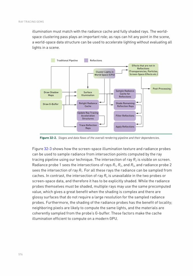
576
illumination must match with the radiance cache and fully shaded rays. The world-space clustering pass plays an important role; as rays can hit any point in the scene, a world-space data structure can be used to accelerate lighting without evaluating all lights in a scene.
Figure 32-2. Stages and data flows of the overall rendering pipeline and their dependencies.
Figure 32-3 shows how the screen-space illumination texture and radiance probes can be used to sample radiance from intersection points computed by the ray tracing pipeline using our technique. The intersection of ray R2 is visible on screen. Radiance probe 1 sees the intersections of rays R1, R2, and R3, and radiance probe 2 sees the intersection of ray R1. For all these rays the radiance can be sampled from caches. In contrast, the intersection of ray R4 is unavailable in the two probes or screen-space data, and therefore it has to be explicitly shaded. While the radiance probes themselves must be shaded, multiple rays may use the same precomputed value, which gives a great benefit when the shading is complex and there are glossy surfaces that do not require a large resolution for the sampled radiance probes. Furthermore, the shading of the radiance probes has the benefit of locality; neighboring pixels are likely to compute the same lights, and the materials are coherently sampled from the probe’s G-buffer. These factors make the cache illumination efficient to compute on a modern GPU.
RAY TRACING GEMS
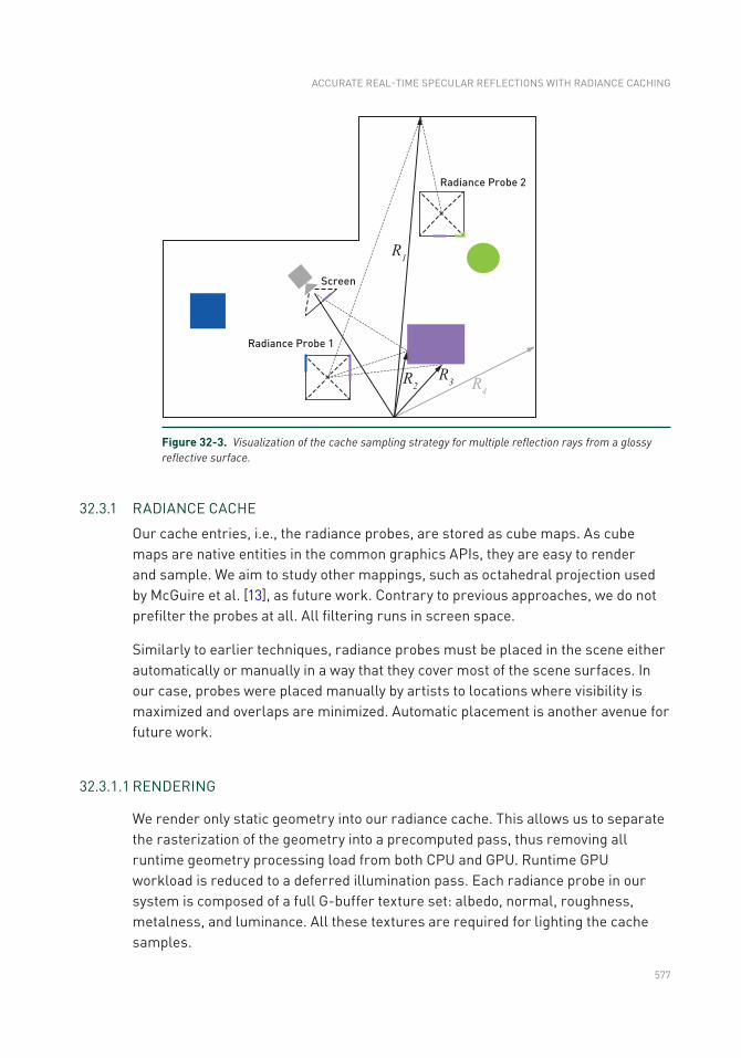
577
32.3.1 RADIANCE CACHE
Our cache entries, i.e., the radiance probes, are stored as cube maps. As cube maps are native entities in the common graphics APIs, they are easy to render and sample. We aim to study other mappings, such as octahedral projection used by McGuire et al. [13], as future work. Contrary to previous approaches, we do not prefilter the probes at all. All filtering runs in screen space.
Similarly to earlier techniques, radiance probes must be placed in the scene either automatically or manually in a way that they cover most of the scene surfaces. In our case, probes were placed manually by artists to locations where visibility is maximized and overlaps are minimized. Automatic placement is another avenue for future work.
32.3.1.1 RENDERING
We render only static geometry into our radiance cache. This allows us to separate the rasterization of the geometry into a precomputed pass, thus removing all runtime geometry processing load from both CPU and GPU. Runtime GPU workload is reduced to a deferred illumination pass. Each radiance probe in our system is composed of a full G-buffer texture set: albedo, normal, roughness, metalness, and luminance. All these textures are required for lighting the cache samples.
R1
R2
R3 R
4
Radiance Probe 1
Radiance Probe 2
Screen
Figure 32-3. Visualization of the cache sampling strategy for multiple reflection rays from a glossy reflective surface.
ACCURATE REAL-TIME SPECULAR REFLECTIONS WITH RADIANCE CACHING
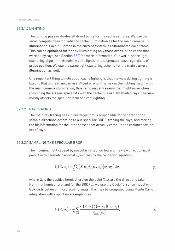
578
32.3.1.2 LIGHTING
The lighting pass evaluates all direct lights for the cache samples. We use the same compute pass for radiance cache illumination as for the main camera illumination. Each full probe in the current system is reilluminated each frame. This can be optimized further by illuminating only those areas in the cache that were hit by rays; see Section 32.7 for more information. Our world-space light clustering algorithm effectively culls lights for the compute pass regardless of probe position. We use the same light clustering scheme for the main camera illumination as well.
One important thing to note about cache lighting is that the view during lighting is fixed to that of the main camera. Albeit wrong, this makes the lighting match with the main camera illumination, thus removing any seams that might arise when combining the screen-space hits with the cache hits or fully shaded rays. The view mostly affects the specular term of direct lighting.
32.3.2 RAY TRACING
The main ray tracing pass in our algorithm is responsible for generating the sample directions according to our specular BRDF, tracing the rays, and storing the hit information for the later passes that actually compute the radiance for the set of rays.
32.3.2.1 SAMPLING THE SPECULAR BRDF
The incoming light caused by specular reflection toward the view direction ωo at point X with geometric normal ωg is given by the rendering equation:
( ) ( ) ( )( ) ,i
o o i i s i o i g iL X , L X , f , dw w w w w w wòW
= ×
(1)
where Ωi is the positive hemisphere on the point X, ωi are the directions taken from that hemisphere, and for the BRDF fs, we use the Cook-Torrance model with GGX distribution of microfacet normals. This may be computed using Monte Carlo integration with importance sampling as
( )( ) ( )( )
( )i o
ni i s i o i g
o oi i
L X fL X
n f1
, ,1, ,w w w w w
ww= W W
×» å (2)
RAY TRACING GEMS
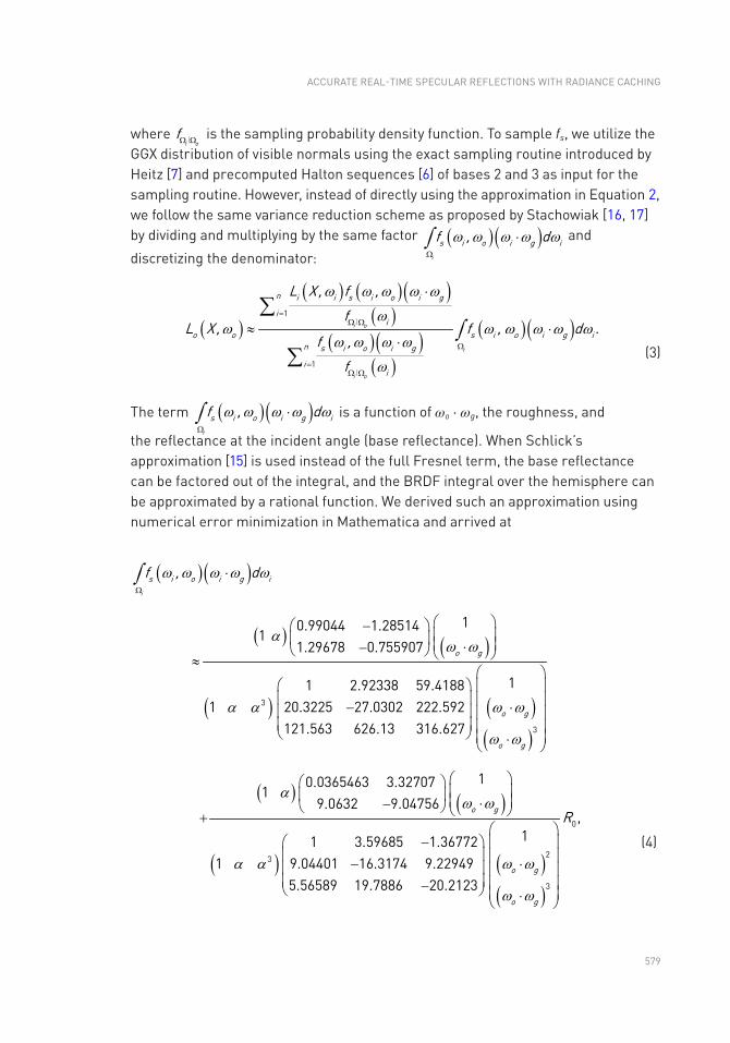
579
where i o
fW W∣ is the sampling probability density function. To sample fs, we utilize the GGX distribution of visible normals using the exact sampling routine introduced by Heitz [7] and precomputed Halton sequences [6] of bases 2 and 3 as input for the sampling routine. However, instead of directly using the approximation in Equation 2, we follow the same variance reduction scheme as proposed by Stachowiak [16, 17] by dividing and multiplying by the same factor ( )( )
i
s i o i g if , dw w w w wòW
× and
discretizing the denominator:
( )
( ) ( )( )( )
( )( )( )
( )( )1
1
.i o
i
i o
n i i s i o i g
ii
o o s i o i g in s i o i g
ii
L X , f ,
fL X , f , d
f ,
f
w w w w w
ww w w w w w
w w w w
w
ò=
W W
W
=W W
×
» ××
å
å
∣
∣
(3)
The term ( )( )i
s i o i g if , dw w w w wòW
× is a function of ωo ⋅ ωg, the roughness, and
the reflectance at the incident angle (base reflectance). When Schlick’s approximation [15] is used instead of the full Fresnel term, the base reflectance can be factored out of the integral, and the BRDF integral over the hemisphere can be approximated by a rational function. We derived such an approximation using numerical error minimization in Mathematica and arrived at
( )( )i
s i o i g if , dw w w w wòW
×
( ) ( )
( ) ( )( )
3
3
10.99044 1.285141
1.29678 0.755907
11 2.92338 59.41881 20.3225 27.0302 222.592
121.563 626.13 316.627
o g
o g
o g
aw w
a a w w
w w
æ öæ - öç ÷ç ÷ ç ÷×-è ø è ø»
æ öæ ö ç ÷ç ÷ ç ÷- ×ç ÷ ç ÷ç ÷ ç ÷è ø ç ÷×è ø
( ) ( )
( ) ( )( )
0
23
3
10.0365463 3.327071
9.0632 9.04756,
11 3.59685 1.367721 9.04401 16.3174 9.22949
5.56589 19.7886 20.2123
o g
o g
o g
R
aw w
a a w w
w w
æ öæ öç ÷ç ÷ ç ÷×-è ø è ø+
æ öæ - ö ç ÷ç ÷ ç ÷- ×ç ÷ ç ÷ç ÷ ç ÷-è ø ç ÷×è ø
(4)
ACCURATE REAL-TIME SPECULAR REFLECTIONS WITH RADIANCE CACHING
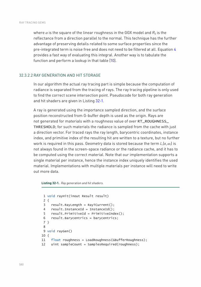
580
where α is the square of the linear roughness in the GGX model and R0 is the reflectance from a direction parallel to the normal. This technique has the further advantage of preserving details related to some surface properties since the pre- integrated term is noise free and does not need to be filtered at all. Equation 4 provides a fast way of evaluating this integral. Another way is to tabulate the function and perform a lookup in that table [10].
32.3.2.2 RAY GENERATION AND HIT STORAGE
In our algorithm the actual ray tracing part is simple because the computation of radiance is separated from the tracing of rays. The ray tracing pipeline is only used to find the correct scene intersection point. Pseudocode for both ray generation and hit shaders are given in Listing 32-1.
A ray is generated using the importance sampled direction, and the surface position reconstructed from G-buffer depth is used as the origin. Rays are not generated for materials with a roughness value of over RT_ROUGHNESS_THRESHOLD; for such materials the radiance is sampled from the cache with just a direction vector. For traced rays the ray length, barycentric coordinates, instance index, and primitive index of the resulting hit are written to a texture, but no further work is required in this pass. Geometry data is stored because the term Li(x, ωi) is not always found in the screen-space radiance or the radiance cache, and it has to be computed using the correct material. Note that our implementation supports a single material per instance, hence the instance index uniquely identifies the used material. Implementations with multiple materials per instance will need to write out more data.
Listing 32-1. Ray generation and hit shaders.
1 void rayHit(inout Result result)
2
3 result.RayLength = RayTCurrent();
4 result.InstanceId = InstanceId();
5 result.PrimitiveId = PrimitiveIndex();
6 result.Barycentrics = barycentrics;
7
8
9 void rayGen()
10
11 float roughness = LoadRoughness(GBufferRoughness);
12 uint sampleCount = SamplesRequired(roughness);
RAY TRACING GEMS
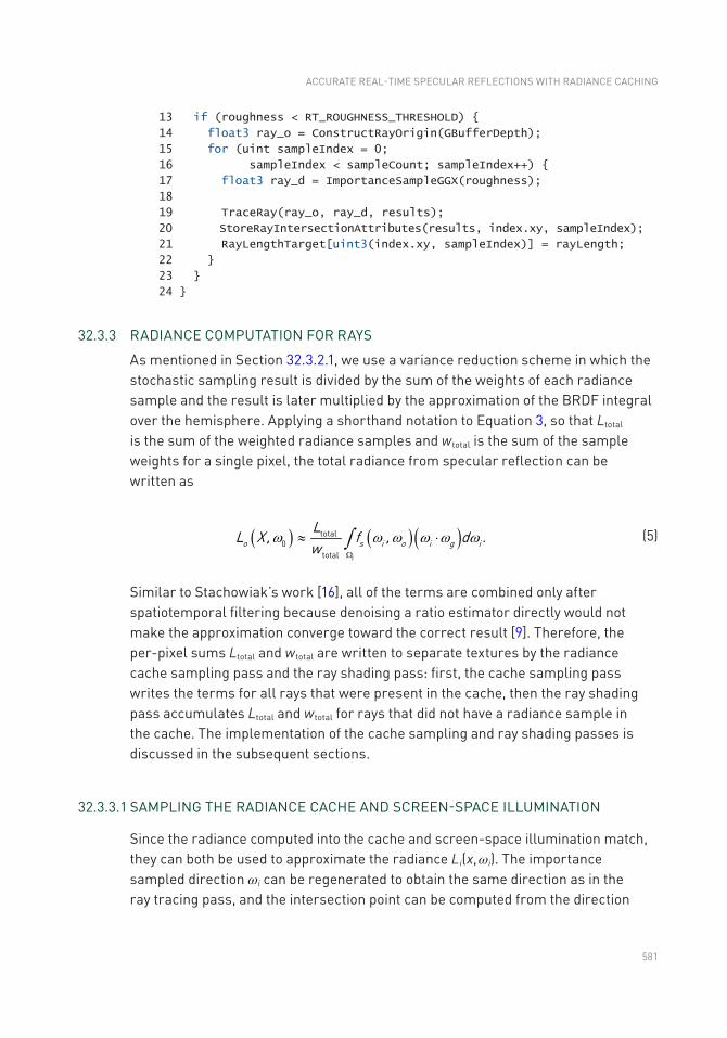
581
13 if (roughness < RT_ROUGHNESS_THRESHOLD)
14 float3 ray_o = ConstructRayOrigin(GBufferDepth);
15 for (uint sampleIndex = 0;
16 sampleIndex < sampleCount; sampleIndex++)
17 float3 ray_d = ImportanceSampleGGX(roughness);
18
19 TraceRay(ray_o, ray_d, results);
20 StoreRayIntersectionAttributes(results, index.xy, sampleIndex);
21 RayLengthTarget[uint3(index.xy, sampleIndex)] = rayLength;
22
23
24
32.3.3 RADIANCE COMPUTATION FOR RAYS
As mentioned in Section 32.3.2.1, we use a variance reduction scheme in which the stochastic sampling result is divided by the sum of the weights of each radiance sample and the result is later multiplied by the approximation of the BRDF integral over the hemisphere. Applying a shorthand notation to Equation 3, so that Ltotal is the sum of the weighted radiance samples and wtotal is the sum of the sample weights for a single pixel, the total radiance from specular reflection can be written as
( ) ( )( )total
0total
.i
o s i o i g i
LL X , f , d
ww w w w w wò
W
» ×
(5)
Similar to Stachowiak’s work [16], all of the terms are combined only after spatiotemporal filtering because denoising a ratio estimator directly would not make the approximation converge toward the correct result [9]. Therefore, the per-pixel sums Ltotal and wtotal are written to separate textures by the radiance cache sampling pass and the ray shading pass: first, the cache sampling pass writes the terms for all rays that were present in the cache, then the ray shading pass accumulates Ltotal and wtotal for rays that did not have a radiance sample in the cache. The implementation of the cache sampling and ray shading passes is discussed in the subsequent sections.
32.3.3.1 SAMPLING THE RADIANCE CACHE AND SCREEN-SPACE ILLUMINATION
Since the radiance computed into the cache and screen-space illumination match, they can both be used to approximate the radiance Li(x, ωi). The importance sampled direction ωi can be regenerated to obtain the same direction as in the ray tracing pass, and the intersection point can be computed from the direction
ACCURATE REAL-TIME SPECULAR REFLECTIONS WITH RADIANCE CACHING
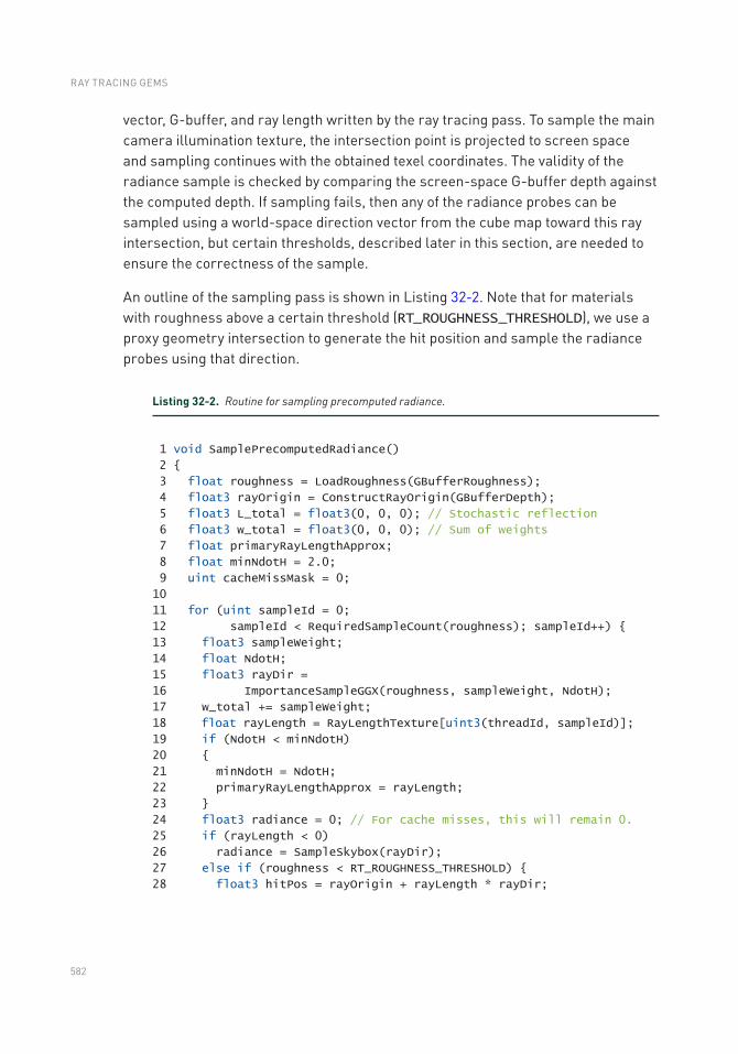
582
vector, G-buffer, and ray length written by the ray tracing pass. To sample the main camera illumination texture, the intersection point is projected to screen space and sampling continues with the obtained texel coordinates. The validity of the radiance sample is checked by comparing the screen-space G-buffer depth against the computed depth. If sampling fails, then any of the radiance probes can be sampled using a world-space direction vector from the cube map toward this ray intersection, but certain thresholds, described later in this section, are needed to ensure the correctness of the sample.
An outline of the sampling pass is shown in Listing 32-2. Note that for materials with roughness above a certain threshold (RT_ROUGHNESS_THRESHOLD), we use a proxy geometry intersection to generate the hit position and sample the radiance probes using that direction.
Listing 32-2. Routine for sampling precomputed radiance.
1 void SamplePrecomputedRadiance()
2
3 float roughness = LoadRoughness(GBufferRoughness);
4 float3 rayOrigin = ConstructRayOrigin(GBufferDepth);
5 float3 L_total = float3(0, 0, 0); // Stochastic reflection
6 float3 w_total = float3(0, 0, 0); // Sum of weights
7 float primaryRayLengthApprox;
8 float minNdotH = 2.0;
9 uint cacheMissMask = 0;
10
11 for (uint sampleId = 0;
12 sampleId < RequiredSampleCount(roughness); sampleId++)
13 float3 sampleWeight;
14 float NdotH;
15 float3 rayDir =
16 ImportanceSampleGGX(roughness, sampleWeight, NdotH);
17 w_total += sampleWeight;
18 float rayLength = RayLengthTexture[uint3(threadId, sampleId)];
19 if (NdotH < minNdotH)
20
21 minNdotH = NdotH;
22 primaryRayLengthApprox = rayLength;
23
24 float3 radiance = 0; // For cache misses, this will remain 0.
25 if (rayLength < 0)
26 radiance = SampleSkybox(rayDir);
27 else if (roughness < RT_ROUGHNESS_THRESHOLD)
28 float3 hitPos = rayOrigin + rayLength * rayDir;
RAY TRACING GEMS
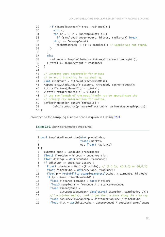
583
29 if (!SampleScreen(hitPos, radiance))
30 uint c;
31 for (c = 0; c < CubeMapCount; c++)
32 if (SampleRadianceProbe(c, hitPos, radiance)) break;
33 if (c == CubeMapCount)
34 cacheMissMask |= (1 << sampleId); // Sample was not found.
35
36
37 else
38 radiance = SampleCubeMapsWithProxyIntersection(rayDir);
39 L_total += sampleWeight * radiance;
40
41
42 // Generate work separately for misses
43 // to avoid branching in ray shading.
44 uint missCount = bitcount(cacheMissMask);
45 AppendToRayShadeInput(missCount, threadId, cacheMissMask);
46 L_totalTexture[threadId] = L_total;
47 w_totalTexture[threadId] = w_total;
48 // Use ray length of the most likely ray to approximate the
49 // primary ray intersection for motion.
50 ReflectionMotionTexture[threadId] =
51 CalculateMotion(primaryReflectionDir, primaryRayLengthApprox);
52
Pseudocode for sampling a single probe is given in Listing 32-3.
Listing 32-3. Routine for sampling a single probe.
1 bool SampleRadianceProbe(uint probeIndex,
2 float3 hitPos,
3 out float3 radiance)
4
5 CubeMap cube = LoadCube(probeIndex);
6 float3 fromCube = hitPos - cube.Position;
7 float distSqr = dot(fromCube, fromCube);
8 if (distSqr <= cube.RadiusSqr)
9 float3 cubeFace = MaxDir(fromCube); // (1,0,0), (0,1,0) or (0,0,1)
10 float hitZInCube = dot(cubeFace, fromCube);
11 float p = ProbabilityToSampleSameTexel(cube, hitZInCube, hitPos);
12 if (p < ResolutionThreshold)
13 float distanceFromCube = sqrt(distSqr);
14 float3 sampleDir = fromCube / distanceFromCube;
15 float zSeenByCube =
16 ZInCube(cube.Depth.SampleLevel (Sampler, sampleDir, 0));
17 // 1/cos(view angle), used to get the distance along the view ray
18 float cosCubeViewAngleRcp = distanceFromCube / hitZInCube;
19 float dist = abs(hitZInCube - zSeenByCube) * cosCubeViewAngleRcp;
ACCURATE REAL-TIME SPECULAR REFLECTIONS WITH RADIANCE CACHING
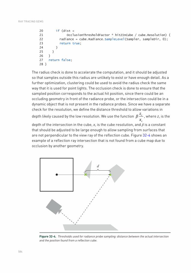
584
20 if (dist <
21 OcclusionThresholdFactor * hitZInCube / cube.Resolution)
22 radiance = cube.Radiance.SampleLevel(Sampler, sampleDir, 0);
23 return true;
24
25
26
27 return false;
28
The radius check is done to accelerate the computation, and it should be adjusted so that samples outside this radius are unlikely to exist or have enough detail. As a further optimization, clustering could be used to avoid the radius check the same way that it is used for point lights. The occlusion check is done to ensure that the sampled position corresponds to the actual hit position, since there could be an occluding geometry in front of the radiance probe, or the intersection could be in a dynamic object that is not present in the radiance probes. Since we have a separate check for the resolution, we define the distance threshold to allow variations in
depth likely caused by the low resolution. We use the function bz
xc
c
, where zc is the
depth of the intersection in the cube, xc is the cube resolution, and β is a constant that should be adjusted to be large enough to allow sampling from surfaces that are not perpendicular to the view ray of the reflection cube. Figure 32-4 shows an example of a reflection ray intersection that is not found from a cube map due to occlusion by another geometry.
Figure 32-4. Thresholds used for radiance probe sampling: distance between the actual intersection and the position found from a reflection cube.
RAY TRACING GEMS
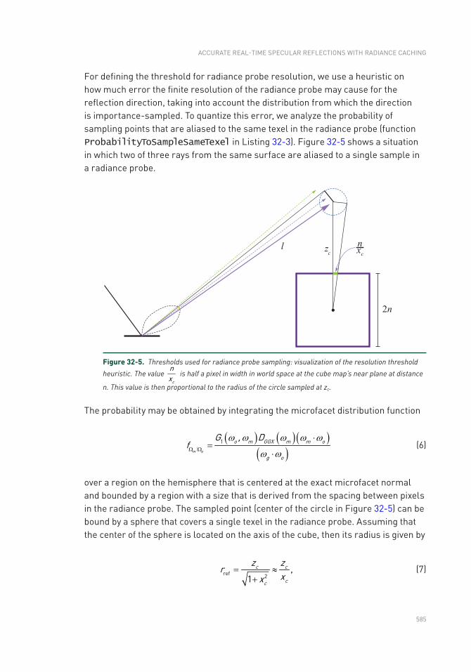
585
For defining the threshold for radiance probe resolution, we use a heuristic on how much error the finite resolution of the radiance probe may cause for the reflection direction, taking into account the distribution from which the direction is importance-sampled. To quantize this error, we analyze the probability of sampling points that are aliased to the same texel in the radiance probe (function ProbabilityToSampleSameTexel in Listing 32-3). Figure 32-5 shows a situation in which two of three rays from the same surface are aliased to a single sample in a radiance probe.
Figure 32-5. Thresholds used for radiance probe sampling: visualization of the resolution threshold
heuristic. The value c
nx
is half a pixel in width in world space at the cube map’s near plane at distance
n. This value is then proportional to the radius of the circle sampled at zc.
The probability may be obtained by integrating the microfacet distribution function
( ) ( )( )( )
1
m o
o m GGX m m o
g o
G , Df
w w w w w
w wW W
×=
×∣
(6)
over a region on the hemisphere that is centered at the exact microfacet normal and bounded by a region with a size that is derived from the spacing between pixels in the radiance probe. The sampled point (center of the circle in Figure 32-5) can be bound by a sphere that covers a single texel in the radiance probe. Assuming that the center of the sphere is located on the axis of the cube, then its radius is given by
ref 2
,1
c c
cc
z zr
xx= »
+
(7)
ACCURATE REAL-TIME SPECULAR REFLECTIONS WITH RADIANCE CACHING
586
where zc is the linear depth of the sample point and xc is the resolution of the radiance probe’s cube map. For cubes, the distance to the near plane, n, cancels out, thus not affecting the calculation. It is possible to generalize the calculation for off-axis sample points, but we are going to neglect it because in cube maps the error is only up to a finite constant from the approximation.
Now we need to evaluate the probability of a reflected ray hitting that sphere. While accurate approximations exist for integrating BRDFs over areas such as the sphere [8], in our case we need only a crude approximation that is efficient to compute. The reflection direction density over the reflected solid angle is given by
( ) ( )( )i o m o
o m GGX mm
i g o
G Ddf f
d1 ,
.4
w w www w wW W W W= =
×∣ ∣
(8)
With the assumption that the projected sphere’s solid angle is small, we can approximate the probability of sampling the texel in the cube map:
( ) ( ) ( )( )
1Pr4
i
o m GGX mi i
S g o
G , DS d
w w ww w
w wòÍW
Î =×
( ) ( )( )
o m GGX m c
cg o
G , D zlx
21 1 1
2
w w w
w w
æ öæ öp ç ÷» - - ç ÷ç ÷× ç ÷è øè ø
(9)
( ) ( )( )
21 ,
4o m GGX m c
cg o
G , D zlx
w w w
w w
æ öp» ç ÷
× è ø
where l is the length of the reflected ray as in Figure 32-5. The first approximation is obtained by doing a single-sample Monte Carlo integration (some value in the domain multiplied by the integration volume, which is the solid angle subtended by a sphere), and the second approximation is obtained by taking the Taylor expansion of the square root term. The threshold can then be defined to anything between 0 and 1. For example, a threshold of 0.1 would mean that if the probability of sampling the texel is 10% or higher, then the cube is rejected, because a single texel does not contain the high- frequency information needed to reconstruct the reflection. However, if the probability is low enough, then the texel is sufficient to reconstruct reflection information. The latter is generally the case for highly rough surfaces, or when the sampled direction is on the tail end of the DGGX distribution. Note that for perfect and near-perfect mirrors this threshold is almost never
RAY TRACING GEMS
587
satisfied, but due to the finite resolution of the view, the samples may still be acceptable. Therefore, when computing the threshold, we clamp the surface’s roughness α to an adjustable minimum value to allow sampling from cubes that have a relatively high resolution. As future work the curvature of the surface and view resolution itself could also be taken directly into account.
32.3.3.2 SHADING CACHE-MISSED RAYS
Covering the whole scene with radiance probes so that every point is visible in some probe would require an extremely high amount of probes in a practical scene, and each one adds overhead to the sampling and relighting passes. Further, we do not include dynamic geometry in the probes, and the resolution of the probes may be too low for some rays, especially for highly smooth surfaces. Therefore, we still need a robust way to reconstruct the radiance for those ray intersections that are not visible in any probe nor in the screen-space illumination texture.
As a fallback we compute the radiance for each of the unshaded samples using a separate compute pass. As the ray tracing pass writes out the geometry instance index, primitive index, and barycentric coordinates, these can be directly used to construct the accurate hit point and query all required data for the illumination pass. Although now it would be possible to use the accurate ray direction for specular highlights, we use the camera direction here to match the specular illumination computed for the radiance cache and screen-space illumination.
To avoid branching within warps/wavefronts based on how many samples require shading, we compact the indices of rays that were cache misses into a separate buffer in the sampling pass. Another compute pass then applies the radiance computation for each of the required rays read from the buffer, so that each thread within a warp/wavefront has the same amount of work to execute. This is essential because for glossy reflections the directions between pixels have high variance, so the cache misses are scattered randomly within large areas and some warps/wavefronts would execute the radiance computation only because one or a few lanes had cache misses.
32.4 SPATIOTEMPORAL FILTERING
The described algorithm provides a crude approximation of the specular environment illumination term. However, due to the low sample counts—one sample per pixel in the extreme case—the resulting approximation is noisy. Therefore, the resulting radiance estimates must be aggressively filtered both spatially and temporally to get rid of the high-frequency noise that results from
ACCURATE REAL-TIME SPECULAR REFLECTIONS WITH RADIANCE CACHING
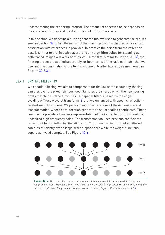
588
undersampling the rendering integral. The amount of observed noise depends on the surface attributes and the distribution of light in the scene.
In this section, we describe a filtering scheme that we used to generate the results seen in Section 32.5. As filtering is not the main topic of this chapter, only a short description with references is provided. In practice the noise from the reflection pass is similar to that in path tracers, and any algorithm suited for cleaning up path traced images will work here as well. Note that, similar to Heitz et al. [9], the filtering process is applied separately for both terms of the ratio estimator that we use, and the combination of the terms is done only after filtering, as mentioned in Section 32.3.3.1.
32.4.1 SPATIAL FILTERING
With spatial filtering, we aim to compensate for the low sample count by sharing samples over the pixel neighborhood. Samples are shared only if the neighboring pixels match in surface attributes. Our spatial filter is based on the edge-avoiding Á-Trous wavelet transform [2] that we enhanced with specific reflection-related weight functions. We perform multiple iterations of the Á-Trous wavelet transformation, where each iteration generates a set of scaling coefficients. These coefficients provide a low-pass representation of the kernel footprint without the undesired high-frequency noise. The transformation uses previous coefficients as an input for the following iteration step. This allows us to accumulate filtered samples efficiently over a large screen-space area while the weight functions suppress invalid samples. See Figure 32-6.
Figure 32-6. Three iterations of one-dimensional stationary wavelet transform while the kernel footprint increases exponentially. Arrows show the nonzero pixels of previous result contributing to the current result, while the gray dots are pixels with zero value. Figure after Dammertz et al. [2].
RAY TRACING GEMS
589
Our implementation follows the previous work by Dammertz et al. [2] and Schied et al. [14]. Each wavelet iteration is performed as a 5 × 5 cross-bilateral filter. The contributing samples are weighted by a function w(P, Q), where P is the current pixel and Q the contributing sample pixel from the sample neighborhood. We calculate the scaling coefficient Si + 1 as
( ) ( ) ( )( ) ( )1 ,iQ
i
Q
h Q w P,Q S QS
h Q w P,QÎW
+
ÎW
= åå
(10)
where ( ) 1 1 1 1 18 4 2 4 8
h Q , , , ,æ ö= ç ÷è ø
is the filter kernel. The weight function w(P, Q) controls
the contribution of the sample Q based on the G-buffer attributes of that sample. The components contributing to this weight function can be categorized into four groups: edge-stopping, roughness, reflection-direction, and ray-length. These four groups are discussed in following sections.
To simplify the weight functions, we define a function fw as a smooth interpolation function between limits a and b as
( ) ( )1 smoothstep ,wf a, b, x a, b, x= - (11)
where smoothstep is the standard cubic Hermite interpolator as provided by shading languages.
32.4.1.1 EDGE-STOPPING WEIGHT
Edge-stopping weights prevent the distribution of samples over geometrical boundaries and take into account the differences between depth and normal values at P and Q. These functions are based on the previous work of Schied et al. [14] with the depth weight wz being
( ) ( )( ) ( )
exp ,zz
z P z Qw
z P P Qs e
æ ö-ç ÷= -ç ÷Ñ × - +è ø
(12)
ACCURATE REAL-TIME SPECULAR REFLECTIONS WITH RADIANCE CACHING
590
where ∇ z(P) is the depth gradient, σz = 1 is a constant value defined by experimentation, and ε = 0.0001 is a small constant value to prevent division by zero. In addition, the weight wn is based on the difference between normals at P and Q and is defined as
( ) ( )( )max 0 ,n
nw , P Qs
= ×n n
(13)
where σn = 32 is again a constant value based on experimentation.
32.4.1.2 ROUGHNESS WEIGHT
Roughness weights simulate the effect of roughness on the reflection lobe. First, we only allow samples that have similar roughness values, and thus a similar shape of reflection lobe, compared to the current pixel:
( ) ( )( ),r w near farw f r , r , r P r Q= -
(14)
where rnear = 0.01 and rfar = 0.1 are constants chosen based on experimentation. Second, we control the filtering radius for the contributing samples based on roughness with weight
( )near far ,d ww f d ,d ,= d
(15)
where dnear = 10 r(P), dfar = 70 r(P), and d = P − Q is the vector from the current pixel position to the sample pixel position.
32.4.1.3 REFLECTION-DIRECTION WEIGHT
A reflection-direction weight makes the filtering kernel anisotropic by scaling it into the direction of the reflection:
( )ˆsatu ,ˆrates bs c cw s s= × +d r
(16)
where r is the reflection direction in screen space, 0.5scs = is a scaling factor, and
0.5bcs = is a scaling bias.
RAY TRACING GEMS
591
32.4.1.4 RAY-LENGTH WEIGHT
The ray-length weight is designed to control the gathering radius as a function of the ray length: the closer the hit point is, the less we want the neighboring samples to contribute. Therefore, the weight wl becomes
( )near far ,l ww f l , l ,= d
(17)
where lnear = 0 and lfar = 10.0 r(P).
Finally, we can combine all the weights into a single function:
( ) ( ) ( ) ( ) ( ) ( ) ( ).z n r d s lw P,Q w P, Q w P,Q w P,Q w P,Q w P,Q w P,Q= (18)
32.4.2 TEMPORAL FILTERING
Unfortunately, the spatial filter is often not sufficient to reach the desired quality. Therefore, in addition to accumulating samples in the pixel neighborhood, we also accumulate them temporally over multiple frames. This is done by interpolating between the current frame samples and the previous temporal results using an exponential moving average:
( ) 11 ,i i iC S Cg g -= - + (19)
where Ci is the current frame output, Ci − 1 is the previous frame output projected using a velocity vector, and Si is the current frame input (i.e., the reflection buffer). Acquiring these velocity vectors for reflections is discussed in further detail in Section 32.4.3. The weight γ denotes the ratio of interpolation between the history data and the current frame and is based on multiple heuristics.
Glossy reflection can have significant color variance between temporal samples. This prevents us from relying on methods based on color values, such as variance clipping, to remove ghosting. Instead, we use a subset of the geometry-based weight functions from Section 32.4.1 to define γ. This is done by first projecting P to generate the sampling location of the contributing sample using a velocity vector and next using that to sample the surface attributes of the previous frame. Thus, we must also save the depth and normal attributes from the G-buffer of the previous frame.
In addition, we include a weight maxrw that is based on the roughness of the
current sample. This is done so that extremely smooth surfaces, such as mirrors,
ACCURATE REAL-TIME SPECULAR REFLECTIONS WITH RADIANCE CACHING
592
disregard unnecessary temporal samples to remove any possible ghosting. This weight is calculated as follows:
( )( )
max maxsmoothstep 0 ,rw ,r , r P=
(20)
where rmax = 0.1 is a constant threshold. Therefore,
( ) ( ) ( )max
0.95 z n r rw P,Q w P,Q w P,Q wg =
(21)
is the total weight used to weight the current and the previous frames.
Nevertheless, ghosting can still appear on planar surfaces with a constant roughness that is large enough not to be clamped by
maxrw but smooth enough for ghosting to be clearly visible. These artifacts are most noticeable with reflections of bright light sources or quickly moving brightly colored objects. Unfortunately, this cannot be solved by geometry weight functions because we cannot account for differences between the objects visible in reflection by comparing the reflector surfaces. Thus, we choose to implement a 5 × 5 filtering kernel for the current reflection result to calculate variance for both incoming light L and the filtered BRDF while using edge-stopping functions to prevent sampling over geometrical boundaries. These are then used for color-space variance clipping of the temporal filtering result Ci, and thus they prevent blending of the temporal results with completely different color values compared to the current frame. This is similar to variance clipping commonly done with temporal antialiasing, only with nonuniform sample weights to prevent sampling over geometrical boundaries.
32.4.3 REFLECTION MOTION VECTORS
Motion vectors need to be adjusted for objects seen through a reflection as the velocity is not just a projection of the object’s velocity onto the screen.
32.4.3.1 UNDERSTANDING THE PROBLEM
To tackle this problem we will start with a fully static system: a camera, a reflector, and an object that is seen in the reflection. In Figure 32-7, light emanates from the object at Po in multiple directions; one of the photons perfectly reflects from the reflector at Ps, 0 and reaches the eye. The object is detected as if it were somewhere along the ray that hit the eye.
RAY TRACING GEMS
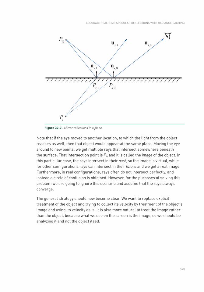
593
Note that if the eye moved to another location, to which the light from the object reaches as well, then that object would appear at the same place. Moving the eye around to new points, we get multiple rays that intersect somewhere beneath the surface. That intersection point is Pi, and it is called the image of the object. In this particular case, the rays intersect in their past, so the image is virtual, while for other configurations rays can intersect in their future and we get a real image. Furthermore, in real configurations, rays often do not intersect perfectly, and instead a circle of confusion is obtained. However, for the purposes of solving this problem we are going to ignore this scenario and assume that the rays always converge.
The general strategy should now become clear. We want to replace explicit treatment of the object and trying to collect its velocity by treatment of the object’s image and using its velocity as is. It is also more natural to treat the image rather than the object, because what we see on the screen is the image, so we should be analyzing it and not the object itself.
Figure 32-7. Mirror reflections in a plane.
ACCURATE REAL-TIME SPECULAR REFLECTIONS WITH RADIANCE CACHING
594
32.4.3.2 DIRECT SOLUTION
A straightforward way of finding Pi, in the sense of least squares, is the solution to the intersection of lines as given by
( )
( )( )s j s j i s j s j s j
j j
s j s j s j o s j
P P
P P
, , , , ,
, , , ,
,
where 2 .
æ ö- = -ç ÷ç ÷
è ø= - -
å åT T
T
I u u I u u
u n n I
(22)
Here, Ps, j are the points on the surface in a local footprint, and us, j are the reflection directions from these points, as shown in Figure 32-7.
The solution for velocity can be obtained after differentiating with respect to time. However, this is cumbersome and requires a significant amount of information.
32.4.3.3 GEOMETRICAL OPTICS APPROACH
If we assume that the reflector point is umbilical, we can simplify the problem significantly. An umbilical point is locally sphere-like, and the problem of finding the image of an object reflected from a spherical surface can be solved by the thin lens equations, which are given by
1 2
1 1 1
, ,
o i
i i i i
o o o o
f r
f z z
x z y zx z y z
= -
Û
= +
Û
= - = -
(23)
where r is the radius of curvature.
32.4.3.4 OBTAINING OPTICAL PARAMETERS
Initial part of this section assumes that the reader is familiar with topics from differential geometry of surfaces. For a thorough discussion on differential geometry we refer the reader to do Carmo’s book [4].
RAY TRACING GEMS
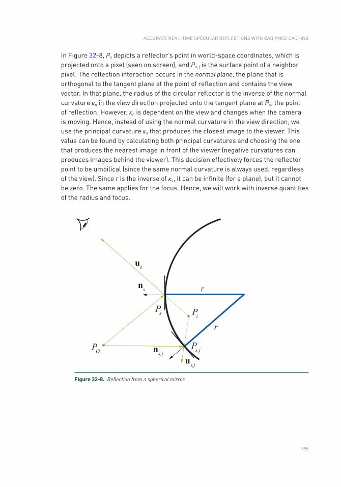
595
In Figure 32-8, Ps depicts a reflector’s point in world-space coordinates, which is projected onto a pixel (seen on screen), and Ps, j is the surface point of a neighbor pixel. The reflection interaction occurs in the normal plane, the plane that is orthogonal to the tangent plane at the point of reflection and contains the view vector. In that plane, the radius of the circular reflector is the inverse of the normal curvature κn in the view direction projected onto the tangent plane at Ps, the point of reflection. However, κn is dependent on the view and changes when the camera is moving. Hence, instead of using the normal curvature in the view direction, we use the principal curvature κs that produces the closest image to the viewer. This value can be found by calculating both principal curvatures and choosing the one that produces the nearest image in front of the viewer (negative curvatures can produces images behind the viewer). This decision effectively forces the reflector point to be umbilical (since the same normal curvature is always used, regardless of the view). Since r is the inverse of κs, it can be infinite (for a plane), but it cannot be zero. The same applies for the focus. Hence, we will work with inverse quantities of the radius and focus.
Figure 32-8. Reflection from a spherical mirror.
ACCURATE REAL-TIME SPECULAR REFLECTIONS WITH RADIANCE CACHING
596
For an orthonormal basis x, y, ns, the reflected object coordinates are
( ) ( ) ( ), , ,o o s o o s o s o sx P P y P P z P P= × - = × - = × -x y n (24)
where Po and Ps are the world-space positions of the reflected object and the reflector, respectively. The image coordinates (xi yi zi)T, which are obtained from the thin lens equations, specify the image position in world space as
i s i i i sP P x y z .= + + +x y n (25)
Note that when this is used as input for the temporal filtering pass of glossy reflections, we want to extend the sample count temporally, i.e., find a sample from the history that was likely sampled from a similar distribution instead of a sample that likely intersected the same position. Therefore, we use an estimate of the intersection of a most likely ray by using the length of the highest-probability ray of the pixel multiplied by the primary reflection direction.
Motion vectors computed with our approach provide better estimates for reprojecting hit positions in curved surfaces than primary hit surface motion vectors, or than approaches that do not take the curvature of the reflecting surface into account. This is shown in Figure 32-9.
RAY TRACING GEMS
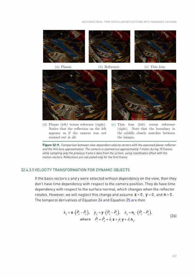
597
Figure 32-9. Comparison between view-dependent velocity vectors with the assumed planar reflector and the thin lens approximation. The camera is zoomed out approximately 1 meter during 10 frames while sampling only the previous frame’s data from the screen, using coordinates offset with the motion vectors. Reflections are calculated only for the first frame.
32.4.3.5 VELOCITY TRANSFORMATION FOR DYNAMIC OBJECTS
If the basis vectors x and y were selected without dependency on the view, then they don’t have time dependency with respect to the camera position. They do have time dependency with respect to the surface normal, which changes when the reflector rotates. However, we will neglect this change and assume 0=x , 0=y , and 0=n . The temporal derivatives of Equation 24 and Equation 25 are then
( ) ( ) ( ), , ,
where .o o s o o s o s o s
i s i i i s
x P P y P P z P P
P P x y z
= × - = × - = × -
= + + +
x y n
x y n
(26)
ACCURATE REAL-TIME SPECULAR REFLECTIONS WITH RADIANCE CACHING
598
From Equation 23, we obtain
2
,ii o
o
zz z
zæ ö
= ç ÷è ø
2
,i o ii o o
o o
z x zx x z
z f zæ ö
= - + ç ÷è ø
(27)
2
.i o ii o o
o o
z y zy y z
z f zæ ö
= - + ç ÷è ø
The velocity of the image point can be readily calculated from Equations 26 and 27, then projected to the screen to obtain the screen-space motion vectors as follows. Given the matrix M that transforms from world coordinates to screen coordinates and the screen coordinates (xss, yss) of the reflector,
( ),0
,3,3 ,1
1 ,i ssi
ssi i
P xv P
yp P
æ öæ ö× æ öç ÷= - × ×ç ÷ ç ÷ç ÷ç ÷× × è øè øè ø
mm
m m
(28)
where m,i denotes the ith row of M. This accounts only for the velocity of the image; the additional velocity component caused by camera movement needs to be added separately. However, since velocity is relative, the camera’s velocity can be subtracted from both the object’s and reflector’s velocities in Equation 26. This makes the matrix M independent of time for this calculation. Another method to calculate the screen- space motion vector is by advancing the image position backward in time with an Euler iteration, projecting it to the screen, and taking the difference in screen space.
32.5 RESULTS
We measured the results of our algorithm in the standard Sponza scene in five different scenarios. We compare against a fully shaded reference, i.e., specular computations without the cache. The scene was fitted with 11 cache sampling points. We used a roughness threshold (RT_MAX_ROUGHNESS) of 0.8. All numbers were captured on an NVIDIA RTX 2080 GPU at a resolution of 2560 × 1440.
In addition to the final illumination and the reflection term images shown in Figure 32-10, we also include images of our reflection mask. The mask is a color-coded visualization of the type of reflection path per pixel. Purple color in the mask denotes the cheapest path: sampling with just a direction vector. Green and orange
RAY TRACING GEMS
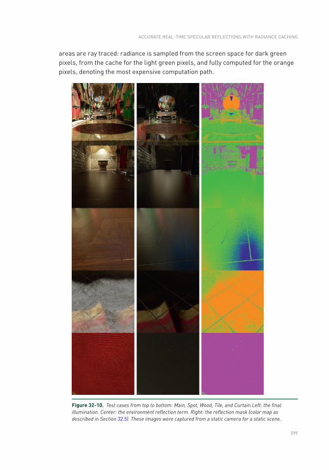
599
areas are ray traced: radiance is sampled from the screen space for dark green pixels, from the cache for the light green pixels, and fully computed for the orange pixels, denoting the most expensive computation path.
Figure 32-10. Test cases from top to bottom: Main, Spot, Wood, Tile, and Curtain.Left: the final illumination. Center: the environment reflection term. Right: the reflection mask (color map as described in Section 32.5). These images were captured from a static camera for a static scene.
ACCURATE REAL-TIME SPECULAR REFLECTIONS WITH RADIANCE CACHING
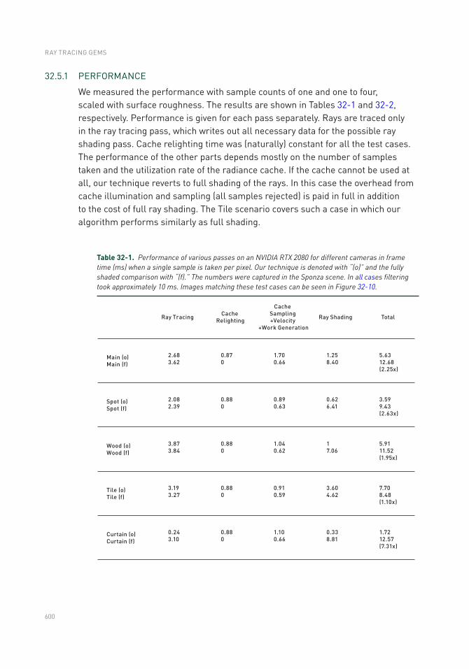
600
32.5.1 PERFORMANCE
We measured the performance with sample counts of one and one to four, scaled with surface roughness. The results are shown in Tables 32-1 and 32-2, respectively. Performance is given for each pass separately. Rays are traced only in the ray tracing pass, which writes out all necessary data for the possible ray shading pass. Cache relighting time was (naturally) constant for all the test cases. The performance of the other parts depends mostly on the number of samples taken and the utilization rate of the radiance cache. If the cache cannot be used at all, our technique reverts to full shading of the rays. In this case the overhead from cache illumination and sampling (all samples rejected) is paid in full in addition to the cost of full ray shading. The Tile scenario covers such a case in which our algorithm performs similarly as full shading.
Table 32-1. Performance of various passes on an NVIDIA RTX 2080 for different cameras in frame time (ms) when a single sample is taken per pixel. Our technique is denoted with “(o)” and the fully shaded comparison with “(f).” The numbers were captured in the Sponza scene. In all cases filtering took approximately 10 ms. Images matching these test cases can be seen in Figure 32-10.
RAY TRACING GEMS
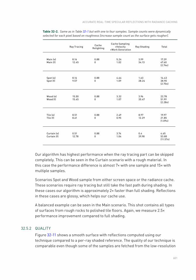
601
Our algorithm has highest performance when the ray tracing part can be skipped completely. This can be seen in the Curtain scenario with a rough material. In this case the performance difference is almost 7× with one sample and 15× with multiple samples.
Scenarios Spot and Wood sample from either screen space or the radiance cache. These scenarios require ray tracing but still take the fast path during shading. In these cases our algorithm is approximately 2× faster than full shading. Reflections in these cases are glossy, which helps our cache use.
A balanced example can be seen in the Main scenario. This shot contains all types of surfaces from rough rocks to polished tile floors. Again, we measure 2.5× performance improvement compared to full shading.
32.5.2 QUALITY
Figure 32-11 shows a smooth surface with reflections computed using our technique compared to a per-ray shaded reference. The quality of our technique is comparable even though some of the samples are fetched from the low-resolution
Table 32-2. Same as in Table 32-1 but with one to four samples. Sample counts were dynamically selected for each pixel based on roughness (increase sample count as the surface gets rougher).
ACCURATE REAL-TIME SPECULAR REFLECTIONS WITH RADIANCE CACHING
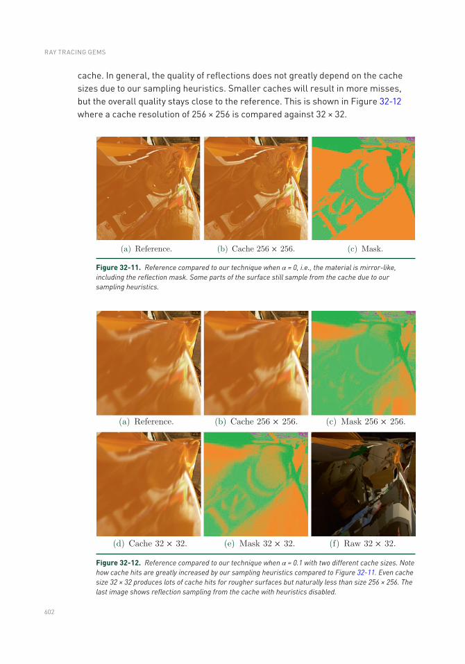
602
cache. In general, the quality of reflections does not greatly depend on the cache sizes due to our sampling heuristics. Smaller caches will result in more misses, but the overall quality stays close to the reference. This is shown in Figure 32-12 where a cache resolution of 256 × 256 is compared against 32 × 32.
Figure 32-11. Reference compared to our technique when α = 0, i.e., the material is mirror-like, including the reflection mask. Some parts of the surface still sample from the cache due to our sampling heuristics.
Figure 32-12. Reference compared to our technique when α = 0.1 with two different cache sizes. Note how cache hits are greatly increased by our sampling heuristics compared to Figure 32-11. Even cache size 32 × 32 produces lots of cache hits for rougher surfaces but naturally less than size 256 × 256. The last image shows reflection sampling from the cache with heuristics disabled.
RAY TRACING GEMS
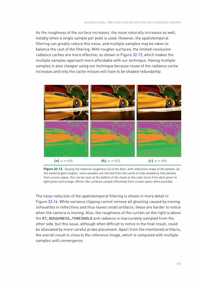
603
As the roughness of the surface increases, the noise naturally increases as well, notably when a single sample per pixel is used. However, the spatiotemporal filtering can greatly reduce this noise, and multiple samples may be taken to balance the cost of the filtering. With rougher surfaces, the limited-resolution radiance caches are more effective, as shown in Figure 32-13, which makes the multiple samples approach more affordable with our technique. Having multiple samples is also cheaper using our technique because reuse of the radiance cache increases and only the cache misses will have to be shaded redundantly.
Figure 32-13. Varying the material roughness (α) of the floor, with reflections maps at the bottom. As the material gets rougher, more samples are fetched from the cache or fully shaded as they deviate from screen space: this can be seen at the bottom of the mask as the color turns from dark green to light green and orange. Mirror-like surfaces sample effectively from screen space when possible.
The noise reduction of the spatiotemporal filtering is shown in more detail in Figure 32-14. While variance clipping cannot remove all ghosting caused by moving silhouettes in reflections and thus leaves small artifacts, these are harder to notice when the camera is moving. Also, the roughness of the curtain on the right is above the RT_ROUGHNESS_THRESHOLD and radiance is inaccurately sampled from the other side, but this issue, although often difficult to notice in the final result, could be alleviated by more careful probe placement. Apart from the mentioned artifacts, the overall result is close to the reference image, which is computed with multiple samples until convergence.
ACCURATE REAL-TIME SPECULAR REFLECTIONS WITH RADIANCE CACHING
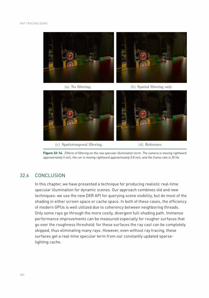
604
Figure 32-14. Effects of filtering on the raw specular illumination term. The camera is moving rightward approximately 5 m/s, the car is moving rightward approximately 0.8 m/s, and the frame rate is 30 Hz.
32.6 CONCLUSION
In this chapter, we have presented a technique for producing realistic real-time specular illumination for dynamic scenes. Our approach combines old and new techniques: we use the new DXR API for querying scene visibility, but do most of the shading in either screen space or cache space. In both of these cases, the efficiency of modern GPUs is well utilized due to coherency between neighboring threads. Only some rays go through the more costly, divergent full-shading path. Immense performance improvements can be measured especially for rougher surfaces that go over the roughness threshold: for these surfaces the ray cast can be completely skipped, thus eliminating many rays. However, even without ray tracing, these surfaces get a real-time specular term from our constantly updated sparse-lighting cache.
RAY TRACING GEMS
605
32.7 FUTURE WORK
There are avenues for improvement in various parts of the algorithm:
> Indirect diffuse: A similar approach can be used to compute indirect diffuse lighting. Rays that miss the cache can get the information from a low-frequency source, such as a hole-filling algorithm.
> Improved cache illumination: Our cache is at the moment illuminated each frame. However, an improved system could be built that only illuminates those cubes, faces, or even samples that are actually used. For example, only the most important cubes could be lit per frame.
> Radiance cache geometry: The implementation described here uses cube maps, i.e., spherical captures, for cache storage. However, this wastes space as the same surfaces can be seen by different cache points. Therefore, we plan to investigate other cache data structures for an improved cache utilization.
> Hole filling: A reflection mask can be very noisy for some surfaces, meaning that some neighboring pixels either sample from cubes or shade the full ray. As shading the full ray is more costly, some of the small holes could be filled based on the neighboring pixel data, especially for rougher surfaces.
> Filtering: The filter presented in this chapter is somewhat expensive for real-time use. In the future we aim to look for lighter filtering solutions that make different trade-offs between quality and performance.
REFERENCES
[1] Crassin, C., Neyret, F., Sainz, M., Green, S., and Eisemann, E. Interactive Indirect Illumination Using Voxel Cone Tracing. Computer Graphics Forum 30, 7 (2011), 1921–1930.
[2] Dammertz, H., Sewtz, D., Hanika, J., and Lensch, H. Edge-Avoiding À-Trous Wavelet Transform for Fast Global Illumination Filtering. In Proceedings of High- Performance Graphics (2010), pp. 67–75.
[3] Debevec, P. Image-Based Lighting. HDRI and Image-Based Lighting, SIGGRAPH Courses, August 2003.
[4] do Carmo, M. P. Differential Geometry of Curves and Surfaces. Prentice Hall Inc., 1976.
[5] Elcott, S., Chang, K., Miyamoto, M., and Metaaphanon, N. Rendering Techniques of Final Fantasy XV. In SIGGRAPH Talks (2016), pp. 48:1–48:2.
[6] Halton, J. H. Algorithm 247: Radical-Inverse Quasi-Random Point Sequence. Communications of the ACM 7, 12 (1964), 701–702.
ACCURATE REAL-TIME SPECULAR REFLECTIONS WITH RADIANCE CACHING
606
[7] Heitz, E. A Simpler and Exact Sampling Routine for the GGX Distribution of Visible Normals. Research report, Unity Technologies, Apr. 2017.
[8] Heitz, E., Dupuy, J., Hill, S., and Neubelt, D. Real-Time Polygonal-Light Shading with Linearly Transformed Cosines. ACM Transactions on Graphics 35, 4 (July 2016), 41:1–41:8.
[9] Heitz, E., Hill, S., and McGuire, M. Combining Analytic Direct Illumination and Stochastic Shadows. In Symposium on Interactive 3D Graphics and Games (2018), pp. 2:1–2:11.
[10] Karis, B. Real Shading in Unreal Engine 4. Physically Based Shading in Theory and Practice, SIGGRAPH Courses, August 2013.
[11] Lagarde, S., and Zanuttini, A. Local Image-Based Lighting with Parallax-Corrected Cubemaps. In SIGGRAPH Talks (2012), p. 36:1.
[12] McGuire, M., and Mara, M. Efficient GPU Screen-Space Ray Tracing. Journal of Computer Graphics Techniques 3, 4 (December 2014), 73–85.
[13] McGuire, M., Mara, M., Nowrouzezahrai, D., and Luebke, D. Real-Time Global Illumination Using Precomputed Light Field Probes. In Symposium on Interactive 3D Graphics and Games (2017), pp. 2:1–2:11.
[14] Schied, C., Kaplanyan, A., Wyman, C., Patney, A., Chaitanya, C. R. A., Burgess, J., Liu, S., Dachsbacher, C., Lefohn, A., and Salvi, M. Spatiotemporal Variance- Guided Filtering: Real-Time Reconstruction for Path-Traced Global Illumination. In Proceedings of High-Performance Graphics (2017), pp. 2:1–2:12.
[15] Schlick, C. An Inexpensive BRDF Model for Physically-based Rendering. Computer Graphics Forum 13, 3 (1994), 233–246.
[16] Stachowiak, T. Stochastic Screen-Space Reflections. Advances in Real-Time Rendering in Games, SIGGRAPH Courses, August 2015.
[17] Stachowiak, T. Stochastic All the Things: Raytracing in Hybrid Real-Time Rendering. Digital Dragons Presentation, 2018.
RAY TRACING GEMS

607
Open Access This chapter is licensed under the terms of the Creative Commons Attribution-NonCommercial-NoDerivatives 4.0 International License (http://creativecommons.org/licenses/by-nc-nd/4.0/), which permits any noncommercial use, sharing, distribution and
reproduction in any medium or format, as long as you give appropriate credit to the original author(s) and the source, provide a link to the Creative Commons license and indicate if you modified the licensed material. You do not have permission under this license to share adapted material derived from this chapter or parts of it.
The images or other third party material in this chapter are included in the chapter's Creative Commons license, unless indicated otherwise in a credit line to the material. If material is not included in the chapter's Creative Commons license and your intended use is not permitted by statutory regulation or exceeds the permitted use, you will need to obtain permission directly from the copyright holder.
ACCURATE REAL-TIME SPECULAR REFLECTIONS WITH RADIANCE CACHING