reliability performance of standby equipment

ca9110828

On

RELIABILITY PERFORMANCE OF STANDBYEQUIPMENT WITH PERIODIC TESTING

Report No 85-267-K

S.H. SimEngineer

Reliability and Statistics SectionOperations Research Department

91602new 82-10

Ontario hydroresearch division

RELIABILITY PERFORMANCE OF STANDBYEQUIPMENT WITH PERIODIC TESTING

Report No 85-267-K

S.H. SimEngineer

Reliability and Statistics SectionOperations Research Department

ABSTRACT

In this report, the reliability performance of standbyequipment subjected to periodic testing is studied.Analytical expressions have been derived forreliability measures, such as the mean accumulatedoperating time to failure, the expected number oftests between two consecutive failures, the mean timeto failure following an emergency start-up and theprobability of failing to complete an emergencymission of a specified duration. These results areuseful for the reliability assessment of standbyequipment such as combustion turbine units of theemergency power supply system, and of the Class IIIpower system at a nuclear generating station.

740672-635-022 813.07 November 29, 198 5 85-267-K

TABLE OF CONTENTS

Page

1. INTRODUCTION 1

2. LIFE CYCLES OF THE STANDBY EQUIPMENT 1

3. PRELIMINARIES 3

3.1 Assumptions 3

3.2 Notations 4

4. RELIABILITY MEASURES 5

4.1 Mean Accumulated Operating Time toFailure 5

4.2 Expected Number of Tests InitiatedBetween Two Consecutive Failures 5

4.3 Expected Time to Failure forEmergency Mission 6

4.4 Mission Failure Probability 75. SPECIAL CASES 8

5.1 Hyperexponential H2 Distribution 95.2 Exponential Distribution 105.3 Erlang E2 Distribution 11

6. NUMERICAL RESULTS 12

6.1 Mean Accumulated Operating Time toFailure 12

6.2 Estimation of MTTF (A"1) 126.3 Expected Time to Failure for Emergency Mission 13

6.4 Mission Failure Probability 14

7. CONCLUSIONS 14

REFERENCES 16

DISTRIBUTION last page

85-267

91601new 82-10

To Mr. F . J . KeeDirector of Research

Ontario hydroresearch division

RELIABILITY PERFORMANCE OF STANDBY EUUIPMENTWITH PERIODIC TESTING

1. INTRODUCTION

Standby equipment is usually tested at regular intervals toensure that it is operable on demand. After the completion ofthe test, it is returned to the standby status. Examples ofsuch equipment are combustion turbine units in the emergencypower supply system, and the Class III power system at a nucleargenerating station/1,2,3,4,5/.

In this study, several reliability measures are defined forstandby equipment. These include the mean accumulated operatingtime to failure, the expected number of tests between twoconsecutive failures, the mean time to failure following anemergency start-up and the probability of failing to complete anemergency mission of a specifiea duration. General equationsare derived for these measures which, in a next step, aresimplified by assuming specific distributions for the times tofailure in the continuous operation mode.

Specifications for standby equipment are likely to includethe starting failure probability and mean time to failure (MTTF)of a similar device in the continuous operation mode. Sincesuch equipment is used in the standby mode, no data oncontinuous operation can be collected to verify the specifiedMTTF. It is shown that an estimate of MTTF can be obtained fromthe knowledge of the mean accumulated operating time to failurein the standby mode, the test duration and the starting failureprobability.

2. LIFE CYCLES OF STANDBY EQUIPMENT

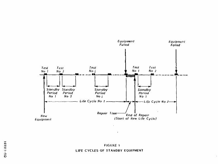
The life of a standjy equipment is made up of cycles. The lifecycles repeat themselves, as shown in Figure 1.

The characteristics of a life cycle are:

(i) A life cycle starts from the instant when theequipment has completed repair, and is as good asnew.

85-267

Equiptnen tFailed

TestNo 1

TestNo 2

TestNo j

Standby StandbyPeriod PeriodNo 1 No 2

StandbyPeriodNo j

Life Cycle No I —

EquipmentFailed

TestNo 1

TestNo 2

StandbyPeriodNo 1

-Life Cycle No 2-

NewEquipment

Repair Time- c . , „End of Repair

(Start of New Life Cycle)

FIGURE 1

LIFE CYCLES OF STANDBY EQUIPMENT

a

(ii) Successive tests are made at regular time inter-vals. During each test, the standby equipment mayfail to start.

(iii) After successful starting, the standby eguipment isoperated for a period of time during which it mayencounter a running failure.

(iv) On successful completion of the test run, the equip-ment is returned to standby status.

(v) A life cycle ends with the detection of either arunning or starting failure.

Note that the emergency duty periods are not indicated in Figure1. They may occur any time between tests; if a failure occursduring a duty period, the life cycle is, of course, terminated.Duty periods are assumed to occur so infrequently (many lifecycles are assumed to pass between two consecutive duty periods)that their effect will be neglected.

3. PRELIMINARIES

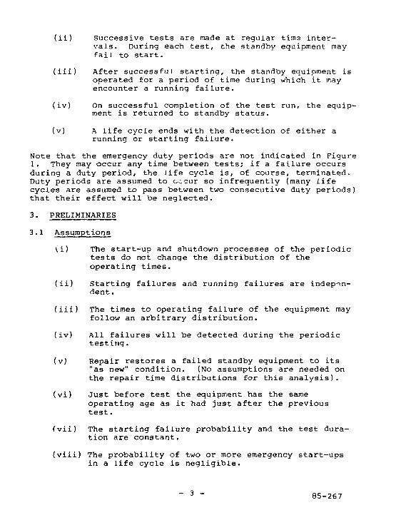
3.1 Assumptions

(i) The start-up and shutdown processes of the periodictests do not change the distribution of theoperating times.

(ii) Starting failures and running failures are indepen-dent.

(iii) The times to operating failure of the equipment mayfollow an arbitrary distribution.

(iv) All failures will be detected during the periodictesting.

(v) Repair restores a failed standby equipment to its"as new" condition. (No assumptions are needed onthe repair time distributions for this analysis).

(vi) Just before test the equipment has the sameoperating age as it had just after the previoustest.

(vii) The starting failure probability and the test dura-tion are constant.

(viii) The probability of two or more emergency start-upsin a life cycle is negligible.

- 3 - 85-267

3.2 Notations

T test duration.

a starting failure probability of the standby equipment.

f(t) probability density function of times to failure of theequipment in the continuous operation mode.

F(t) probability distribution of times to failure of theequipment in the continuous operation mode.

X"1 mean time to failure (MTTF) of the equipment in thecontinuous operation mode, and is the.'efore the mean ofF(t).

v coefficient of variation of times to failure of theequipment in the continuous operation mode.

L accumulated operating time to failure of the standbyequipment.

X residual lifetime of the standby equipment following anemergency start-up.

N s number of standby periods in a life cycle.

N t number of tests initiated in a life cycle.

U unavailability of the standby equipment due to repairs.

E(D) expected downtime of the standby equipment due torepairs.

I indicator variable. Note that

1 if an emergency occursI =

0 if no emergency occurs

Aj the emergency event occurs during the jth standbyperiod of the equipment's life cycle.

P(T|I=1) probability that the standby equipment will fail tooperate successfully for an emergency mission of Thours' duration.

E(x|l=l) expected time to failure following an emergency start-up.

- 4 - 85-267

4. RELIABILITY MEASURES

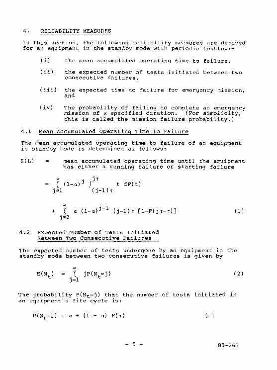
In this section, the following reliability measures are derivedfor an equipment in the standby mode with periodic testing:-

(i) the mean accumulated operating time to failure,

(ii) the expected number of tests initiated between twoconsecutive failures,

(iii) the expected time to failure for emergency mission,and

(iv) The probability of failing to complete an emergencymission of a specified duration. (For simplicity,this is called the mission failure probability.)

4.1 Mean Accumulated Operating Time to Failure

The mean accumulated operating time to failure of an equipmentin standby mode is determined as follows:

E(L) = mean accumulated operating time until the equipmenthas either a running failure or starting failure

= I (l-a)j ^ t dF(t)j=l (j-l)t

+ I a ( 1 - a ) ^ 1 ( J - 1 ) T [ I - F ( J T - T ) ] (1)

j=2

4.2 Expected Number of Tests InitiatedBetween Two Consecutive Failures

The expected number of tests undergone by an equipment in thestandby mode between two consecutive failures is given by

E(N.) = ? jP(N =j) (2)* j=l

The probability P(Nt=j) that the number of tests initiated inan equipment's life cycle is:

P(N<.=1) = a + (1 - a) P(T) j = l

" 5 - 85-267

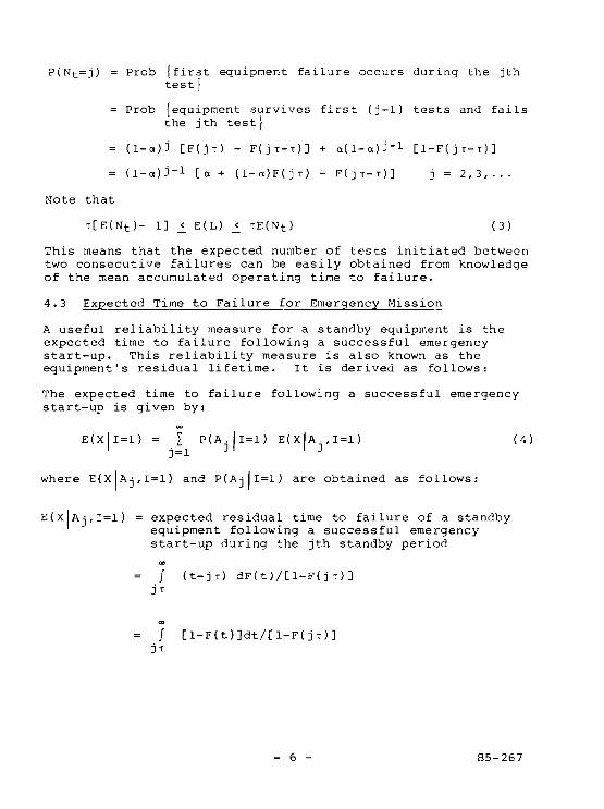
P(Nt=j) = Prob (first equipment failure occurs during the jthtest f

= Prob (equipment survives first (j-1) tests and failsthe jth test}

= (l-a)J [F(JT) - F ( J T - T ) ] + a(l-a):-1 [ I - F ( J T - T ) ]

= (l-a)^-1 [a + (I-O)F(JT) - F ( J T - T ) ] j = 2,3,...

Note that

T[E(Nt)- 1] _<_ E{L) <_ TE(Nt) (3)

This means that the expected number of tests initiated betweentwo consecutive failures can be easily obtained from knowledgeof the mean accumulated operating time to failure.

4.3 Expected Time to Failure for Emergency Mission

A useful reliability measure for a standby equipment is theexpected time to failure following a successful emergencystart-up. This reliability measure is also known as theequipment's residual lifetime. It is derived as follows:

The expected time to failure following a successful emergencystart-up is given by:

E(X|I=1) = I P(A.|l=l) E(XJA.,I=1) (4)I j = 1 3 1 1 3

where E(XJAj,1=1) and P(Ajll=l) are obtained as follows:

E(x|Aj,I=l) = expected residual time to failure of a standbyequipment following a successful emergencystart-up during the jth standby period

00

= / (t-jl) dF(t)/[l-F(JT)]JT

- 6 - 85-267

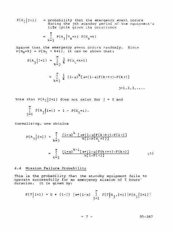
P(A-;|l = l) = probability that the emergency event occursduring the jth standby period of the equipment'slife cycle given its occurrence

= I P(A.IN =k) P ( N = k )k=j Jl S S

Assume that the emergency event occurs randomly. SinceP(Ns=k) = P(Nt = k+1), it can be shown that:

P(A.ll = l) = I ^ P(N.=k+l)^ k=j k t

= I £ U-a)k[a+(l-a)F(kT+T)-F(kT)]k=j

j = l , 2 , 3 ,

Note t h a t P ( A j | l = l ) does not e x i s t fo r j = 0 and

00

I P ( A _ . | l = l ) = 1 - P ( N t = l ) .

Normalizing, one obtains

| ,. y (1-a) [ g+( l-g)F(k T+i)-F(k T) ]jI ' = k^. k[l-P(Nt=l)]

r (l-a)k"1[a+(l-a)F(kT+T)-F{kT)]

4.4 Mission Failure Probability

This is the probability that the standby equipment fails tooperate successfully for an emergency mission of T hours'duration. It is given by:

ao

P(T|I = 1) = U + (1-U) (a+(l-a) I P(TIA.,1 = 1) }p(A . 11=1)

- 7 - 35-267

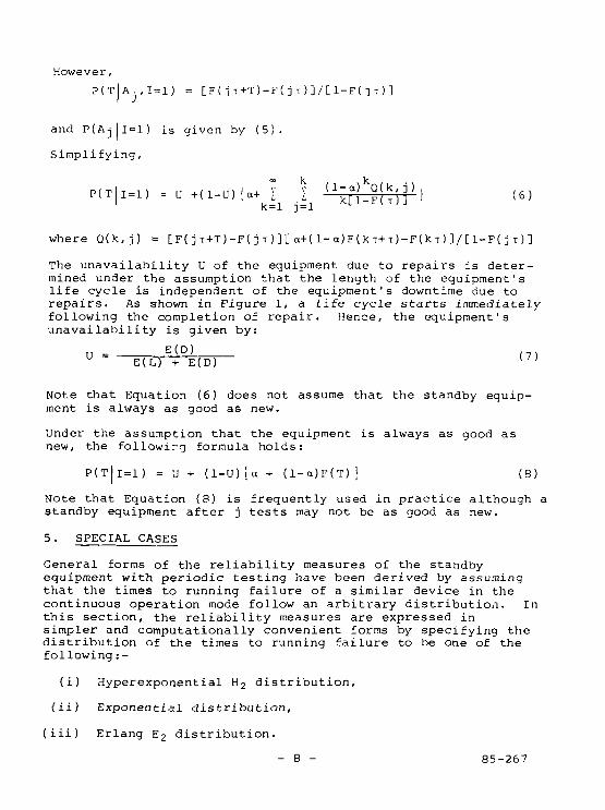
However,

?(TJAj(I=l) = [F(JT+T)-F(ji)]/[1-F(jt)]

and P(Aj|l=l) is given by (5).

Simplifying,

P(T|I = 1) , U +(1-U)(a+ I \ nil£QF[*')i) \ (6)

where Q(k,j) = [F(jT+T)-F(jT)][a+(1-a)F(kT+i)-F(kT)]/[1-F(jT)]

The unavailability U of the equipment due to repairs is deter-mined under the assumption that the length of the equipment'slife cycle is independent of the equipment's downtime due torepairs. As shown in Figure 1, a life cycle starts immediatelyfollowing the completion of repair. Hence, the equipment'sunavailability is given by:

U =(7)

EC) + E(D) { "Note that Equation (6) does not assume that the standby equip-ment is always as good as new.

Under the assumption that the equipment is always as good asnew, the following formula holds:

P(T|l=l) = U + (l-U)io + (l-a)F(T)} (8)

Note that Equation (8) is frequently used in practice although astandby equipment after j tests may not be as good as new.

5. SPECIAL CASES

General forms of the reliability measures of the standbyequipment with periodic testing have been derived by assumingthat the times to running failure of a similar device in thecontinuous operation mode follow an arbitrary distribution. Inthis section, the reliability measures are expressed insimpler and computationally convenient forms by specifying thedistribution of the times to running failure to be one of thefollowing:-

(i) Hyperexponential H2 distribution,

(ii) Exponential distribution,

(iii) Erlang E2 distribution.

- 8 - 85-267

5.1 Hyperexponential H? Distribution

The probability density function is given by

-X,t -X-tf(t) = BXj e + (l-6)X2e t _>. 0

where 0 <_ 8 £ 1, X i >_ 0 and X2 s °- T n e parameters 3, \j and x2

Can be expressed in terms of mean (1/K) and variance (a2) oftimes to running failure as given below:

Xi = 2X,X2 = X/(2v -1), and8 = 4(v2-l)/(4v2-3)

where v = coefficient of variation= \a.

The hyperexponential distribution has the following characteris-tics:

- the coefficient of variation is greater than one;

- it has a decreasing hazard rate function.

Since F(t) is known explicitly, the reliability measures, asgiven by equations (1), (2), (4) and (6), can be simplified.After performing some algebraic manipulations, the followingexpressions are obtained for the equipment in the standby mode:

(i) The mean accumulated operating time to failure is

E(L) = B(l-a)- X, T

)+

A [l-(l-a)e l 1 X [l-(l-a)e 2 ]1 2

(ii) The expected number of tests between two consecutivefailures is

_

" 9 - 85-267

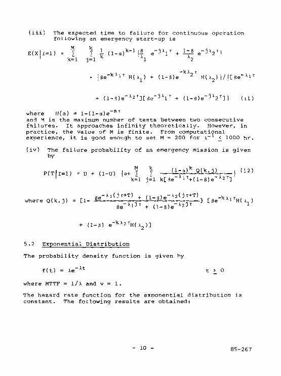
(iii) The expected time to failure for continuous operationfollowing an emergency start-up is

E(X|I=1) ~- \ \ i(l-a)W(l e ^ V + e ^ V }1 k=l j=l K Al A2

, , - k X _ T

• l S e - k X l T H { X 1 ) + ( l - B ) e 2 H ( X . , ) 1 / | [ B e " x 1 T

+ (l-S)e"X2T][Se"jXlT + (l-S)e~jX2T]} (11)

where H(a) = l-(l-a)e~aT

and M is the maximum number of tests between two consecutivefailures. It approaches infinity theoretically. However, inpractice, the value of M is finite. From computationalexperience, it is good enough to set M = 200 for \~l <_ 1000 hr.

(iv) The failure probability of an emergency mission is givenby

i-i) - u + (i-u) {*+ j i ( 1: a ) k Q ( k-J )x } (12)

k=l j = l k [ B e " A l T + ( l - 8 ) e ~ A 2 T ]

where Q(k,j) = [1-

+ (1-S) e"kX2TH(X2)]

5.2 Exponential Distribution


f(t) = \e~Xt t >_ 0

where MTTF = l/X and v = 1.

The hazard rate function for the exponential distribution isconstant. The following results are obtained:

- 10 - 85-267

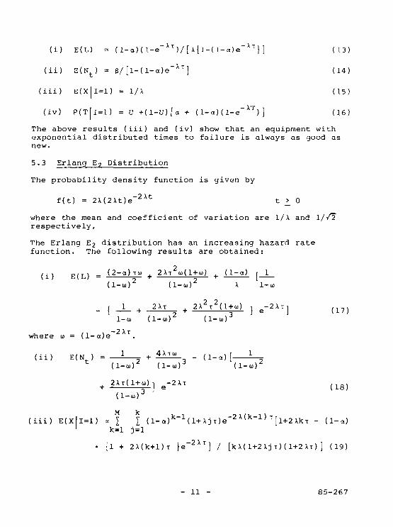
(i) E(L) = (l-ct)O.-e XT)/[\{1-(1-a)e X T } ] (13)

(ii) E(Nt) = 0/[l-(l-a)e~XT] (14)

(iii) E(x|l=l) = I/A (15)

(iv) P(T|l=l) = U +(1-U)[a + (l-ot)(l-e"XT) ] (16)

The above results (iii) and (iv) show that an equipment withexponential distributed times to failure is always as good asnew.

5 . 3 Erlang E? Distribution


f ( t ) = 2A(2At)e~2 X t t _> 0

where the mean and coefficient of variation are I/A and 1//2"respectively.

The Erlang E2 distribution has an increasing hazard ratefunction. The following results are obtained:

(i) E(L) = + +

(1-u)2 (1-iu)2 \ 1-u)

_ ^ + +

1-u (1-w) (1-co)

where 10 = (l-a)e~2Xx.

E ( N )

k"1(l+AJT)e"2X(k"1)T[(iii) E(X|I=1) = I I (l-a)k"1(l+AJT)e"2X(k"1)T[l+2Akr - (1-a)1 k=l j=l

• {l + 2A(k+l)x }e~2XT] / [kA(l+2AJT)(l+2Ax) ] (19)

- 11 - 85-267

(iv) P(T|l = l) - U +U-U){a + V V ^-<x) UU.J ; ( 2 0 )1 k=l j=l k(l+2Ax)e

where Q(k,j) = e 2 A X r [l+2Xkt - (1-a) {1+2X(k+1)t }e

jt+T) e-2XTiJ[X 1+2Xjt

6. NUMERICAL RESULTS

Consider a standby combustion turbine unit with operating andmaintenance characteristics as described in this report.

6.1 Mean Accumulated Operating Time to Failure

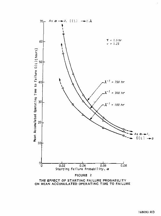
The mean accumulated operating time to failure of the equipmentin standby mode is computed for specified values of X"1, T, aand v. The results are shown in Figures 2 to 6.

As expected. Figure 2 shows that the mean accumulated operatingtime to failure decreases significantly with increasing valuesof starting failure probability.

Figure 3 shows that the mean accumulated operating time tofailure increases significantly with increasing values oftest duration.

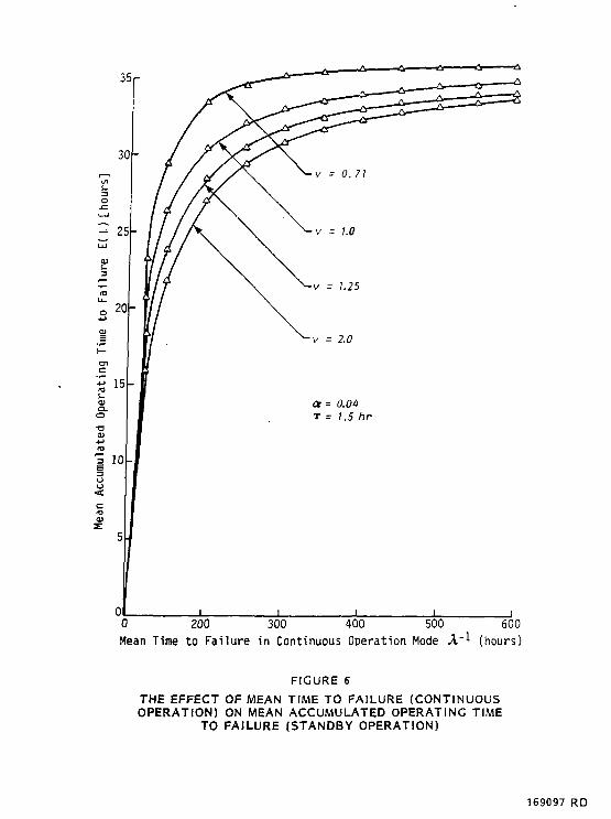
Figures 4, 5 and 6 show that the mean accumulated operating timeto failure increases with increasing values of the mean time tofailure of the same equipment in continuous operation mode. Therate of increase of E(L) decreases with increasing X"1. Thismeans that as \~l becomes large (eg, X > 800 h), the startingfailure becomes a dominant failure cause.

6.2 Estimation of MTTF (X~ x)

In practice, the following information can be extracted fromrecorded data of the equipment in standby mode:

(i) mean accumulated operating time to failure(ii) starting failure probability,(iii) average test duration.

The mean time to failure for such an equipment in the continuousoperation mode can be easily estimated from Figure 6. As anexample, let

- 12 - 85-267

a = 0.04,T = 1.5 h, and

E(L) = 27.5 h

The following results are obtained:

x- l =

90 h120 h

for v = 0.71for v = 1. 00

175 h for v = 1.25

220 h for v = 2.00

(Erlang E2 distribution)(Exponential distribution)(Hyperexponential H2 distri-bution)(Hyperexponential H2 distri-bution)

Note that the coefficient of variation of times to failureaffects the estimated value of X"1 significantly.

6.3 Expected Time to Failure for Emergency Mission

The mean time E(X 1=1) to failure of the standby equipmentfollowing an emergency start-up is computed for specified valuesof X , a, x, and v. The results are tabulated in Table 1. Asexpected, an equipment with exponential times to failure is notaffected by the periodic test policy and is as good as new. Foran equipment with increasing (decreasing) hazard rate function,E(x|l=l) is less (greater) than X"1.

TABLE 1

Expected Time to Failure of Standby EquipmentFollowing an Emergency Start-Up

(a = 0.04 and T = 1.5 hr)

Mean timeto failureof newequipment.A"1(hours)

100200300400500600700800

Expected timemission

v = 1.25(Hyperexponential)

107.5208.7309.1409.4509.5609.6709.7809.7

to failure for emergencyE(X 1 = 1 ) (hours)

v = 1.0(Exponential)

100200300400500600700800

v = J.//7(Erlang E2)

89.9186.7285.1384.2483.5583.1682.7782.4

- 13 - 85-267

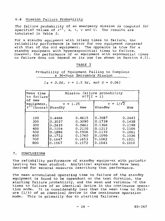
6 ,.4 Mission Failure Probability

The failure probability of an emergency mission is computed forspecified values of \ , a, T, V and U. The results aretabulated in Table 2.

For a standby equipment with Erlang times to failure, thereliability performance is better for new equipment comparedwith that of the old equipment. The opposite is true for astandby equipment with hyperexponential times to failure.However, the performance of an equipment with exponential timesto failure does not depend on its age (as shown in Section 4.2).

TABLE 2

Probability of Equipment Failing to Completea 36-Hour Emergency Mission

(a = 0.04, T = 1.5 hr, and U = 0.06)

Mean timeto failureof newequipment,X-1(hours)

100200300400500600700800

V

Standby

0.44660.30370.24350.21040.18960.17520.16470.1567

Mission failure probabilityP(T| I

1= 1.25

New

0.46150.30900.24610.21200.19060.17600.16530.1572

= 1)

v =Standby

0.30870.17390.13660.12130.11350.10900.10620.1043

= 1//2

0.0.0.0.0.0.0.0.

New

24451438119811061061103610211010

7. CONCLUSIONS

The reliability performance of standby equipment with periodictesting has been studied. Analytical expressions have beenderived for several measures describing that performance.

The mean accumulated operating time to failure of the standbyequipment is found to be dependent on the test duration, thestarting failure probability, and the mean and variance of thetimes to failure of an identical device in the continuous opera-tion mode. It is considerably less than the mean time to fail-ure (l/A) of an identical device in the continuous operationmode. This is primarily due to starting failures.

- 14 - 85-267

Bounds of the mean accumulated operating time to failure ofstandby equipment can be obtained from the knowledge of theexpected number of tests between two consecutive failures.

The expected time to failure (E(XII=1) and the mission failureprobability P(TJI=1) of the standby equipment following anemergency start-up are found to be greatly dependent on theprobability distribution F(t) of the times to failure of anidentical device in continuous operation mode. The followingconclusions can be drawn:-

(a) E(xll=l) > l/X for equipment with decreasing hazard ratefunction,

E(xll=l) = 1/X for equipment with constant hazard ratefunction, and

E(XJl=l) < l/X for equipment with increasing hazard ratefunction.

(b) The mission failure probability of a standby equipment islower than that of a new equipment for decreasing hazardrate function. The opposite is true for increasing hazardrate function. Such differences diminish as the mean timeto failure (l/X) becomes larger.

Approved: Submitted:

J.G. Cassan S.H. SimManager EngineerOperations Research Reliability & Statistics

Section

Sii£:djb/l}h

- 15 - 85-267

REFERENCES

1. Halinaty, M.W. (1981), Running Failure Patterns of CTU's inStandby Operation at Ontario Hydro's Nuclear GenerationFacilities, Ontario Hydro Desig.i and Development DivisionReport No 81367, Aug 1981.

2. Mankamo, T. and U. Pulkkinen (1982), Dependent Failures ofDiesel Generators, Nuclear Safety 23, 32-43.

3. Sim, S.H. (1985), Unavailability Analysis of PeriodicallyTested Components of Dormant Systems, IEEE Transactions onReliability R-34, 88-91.

4. Sim, S.H. (1984), Availability Model of Periodically TestedStandby Combustion Turbine Units, Institute of IndustrialEngineers Transactions 16, 288-291.

5. Sim, S.H. (1982), Reliability Models of Redundant StandbySystems with Multiple Repair Teams, Research DivisionReport No 82-559-K.

- 16 - 85-267

f—1ini.

hoi

lure

to

Fai

01S1—

"ati

ng

Ope

i

•a<u1O

3

Acc

uile

an

2 .

7

6

50

40

30

20

10

0

_ As a—t-0, E ( L)

tt

\ \

\ \

\ \»w\

— 7/A

w

T = 7. 5 hrv - 1.25

-A'1 = 750 hr

rX~' = 300 hr

/

/-X1 = 100 hr/

^ ^

I i

». As a-•-•* E ( L

0 0.02 0.04 0.06 0.08Starting Failure Probability, a

FIGURE 2

THE EFFECT OF STARTING FAILURE PROBABILITYON MEAN ACCUMULATED OPERATING TIME TO FAILURE

169093 RD

A ' = 750 hr

X'1 = 300 hr

1.0 1.5 2.0Test Duration T (hours)

2.5

FICURE 3

THE EFFECT OF TEST DURATION ON MEANACCUMULATED OPERATING TIME TO FAILURE

169094 RD

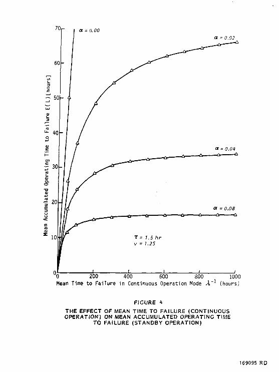
a = 0.02

0 200 400 600 800 1000Mean Time to Failure in Continuous Operation Mode A"1 (hours)

FICURE t

THE EFFECT OF MEAN TIME TO FAILURE (CONTINUOUSOPERATION) ON MEAN ACCUMULATED OPERATING TIME

TO FAILURE (STANDBY OPERATION)

169095 RD

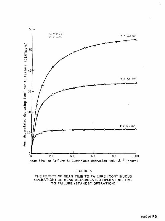
- 2.5 hr

0 200 400 600 800 1000

Mean Time to Failure in Continuous Operation Mode A'* (hours)

FIGURE 5



169096 RD

35

00 200 300 400 500 600Mean Time to Failure in Continuous Operation Mode A' 1 (hours)

FIGURE 6



169097 RD

reliability performance of standby equipment

Documents