reliability analysis process and - open metu
TRANSCRIPT
RELIABILITY ANALYSIS PROCESS AND RELIABILTY IMPROVEMENT OF
AN INERTIAL MEASUREMENT UNIT (IMU)
A THESIS SUBMITTED TO THE GRADUATE SCHOOL OF NATURAL AND APPLIED SCIENCES
OF MIDDLE EAST TECHNICAL UNIVERSITY
BY
ÖZLEM ÜNLÜSOY
IN PARTIAL FULFILLMENT OF THE REQUIREMENTS FOR
THE DEGREE OF MASTER OF SCIENCE IN
AEROSPACE ENGINEERING
SEPTEMBER 2010

Approval of the thesis:
RELIABILITY ANALYSIS PROCESS AND RELIABILTY IMPROVEMENT OF AN INERTIAL MEASUREMENT UNIT (IMU)
submitted by ÖZLEM ÜNLÜSOY in partial fulfillment of the requirements for the degree of Master of Science in Aerospace Engineering Department, Middle East Technical University by, Prof. Dr. Canan Özgen _____________________ Dean, Graduate School of Natural and Applied Sciences Prof. Dr. Ozan Tekinalp _____________________ Head of Department, Aerospace Engineering Prof. Dr. Nafiz Alemdaroğlu _____________________ Supervisor, Aerospace Engineering Dept., METU Examining Committee Members: Prof. Dr. Serkan Özgen _____________________ Aerospace Engineering Dept., METU Prof. Dr. Nafiz Alemdaroğlu _____________________ Aerospace Engineering Dept., METU Assoc. Prof. Dr. Yasemin Serin _____________________ Industrial Engineering Dept., METU Assoc. Prof. Dr. Barış Sürücü _____________________ Statistics Dept., METU Asst. Prof. Dr. Ali Türker Kutay _____________________ Aerospace Engineering Dept., METU
Date: 02.09.2010

iii
I hereby declare that all the information in this document has been obtained and presented in accordance with academic rules and ethical conduct. I also declare that, as required by these rules and conduct, I have fully cited and referenced all material and results that are not original to this work.
Name, Last Name:
Signature:
iv
ABSTRACT
RELIABILITY ANALYSIS PROCESS AND RELIABILTY IMPROVEMENT
OF AN INERTIAL MEASUREMENT UNIT (IMU)
Ünlüsoy, Özlem
M.Sc., Department of Aerospace Engineering
Supervisor : Prof. Dr. Nafiz Alemdaroğlu
September 2010, 94 pages
Reliability is one of the most critical performance measures of guided
missile systems. It is directly related to missile mission success. In order to have a
high reliability value, reliability analysis should be carried out at all phases of the
system design. Carrying out reliability analysis at all the phases of system design
helps the designer to make reliability related design decisions in time and update
the system design.
In this study, reliability analysis process performed during the conceptual
design phase of a Medium Range Anti-Tank Missile System Inertial Measurement
Unit (IMU) was introduced. From the reliability requirement desired for the
system, an expected IMU reliability value was derived by using reliability
allocation methods. Then, reliability prediction for the IMU was calculated by
using Relex Software. After that, allocated and predicted reliability values of the
IMU were compared. It was seen that the predicted reliability value of the IMU did
not meet the required reliability value. Therefore, reliability improvement analysis
was carried out.
Keywords: reliability prediction, reliability allocation, redundancy, Inertial
Measurement Unit, medium range anti-tank missile
v
ÖZ
ATALETSEL ÖLÇÜM BİRİMİ (AÖB) GÜVENİLİRLİK HESAPLAMASI VE
GÜVENİLİRLİK İYİLEŞTİRMESİ
Ünlüsoy, Özlem
Yüksek Lisans, Havacılık ve Uzay Mühendisliği Bölümü
Tez Yöneticisi : Prof. Dr. Nafiz Alemdaroğlu
Eylül 2010, 94 sayfa
Güdümlü füzeler için en kritik performans kriterlerinden biri güvenilirliktir.
Sistem güvenilirliği doğrudan füze görev başarımını etkilemektedir. Yüksek
güvenilirlik değeri elde edebilmek için, güvenilirlik analizleri sistem tasarımının
bütün aşamalarında gerçekleştirilmelidir. Tüm tasarım boyunca güvenilirlik
analizlerinin gerçekleştirilmesi, güvenilirlik tabanlı tasarım kararları alınması ve
sistem güncellemelerinin yapılması sırasında tasarımcıya yardımcı olur.
Bu çalışmada, Orta Menzilli Tanksavar Füze Sistemi Ataletsel Ölçüm
Birimi (AÖB) için tasarım aşamasında güvenilirlik analizi yapılmıştır. Güvenilirlik
atama yöntemleri kullanılarak sistem güvenilirlik gereksiniminden beklenen AÖB
güvenilirlik gereksinimi çıkartılmıştır. Daha sonra, Relex paket programı
kullanılarak AÖB güvenilirlik değeri hesaplanmıştır. Bu çalışmalardan sonra,
AÖB beklenen güvenilirlik değeri ve hesaplanan güvenilirlik değeri
karşılaştırılmıştır. Karşılaştırma sonucunda, hesaplanan güvenilirlik değerinin
beklenen AÖB güvenilirlik değerini karşılamadığı görülmüştür. Bu nedenle,
güvenilirlik iyileştirme çalışması yapılmıştır.
Anahtar Kelimeler: güvenilirlik tahmini, güvenilirlik ataması, yedekleme,
Ataletsel Ölçüm Birimi (AÖB), orta menzilli tanksavar füze

vi
to my precious family
and
beloved husband
for their love, care and support

vii
ACKNOWLEDGEMENTS
I would like to express my gratitude to my supervisor Prof. Dr. Nafiz
Alemdaroğlu for his vision, encouragement and support in this study.
I must also express my appreciation to my superiors at Roketsan Inc., Dr.
Sartuk Karasoy, Bülent Semerci, Barlas Ortaç and Ahmet Aydoğan for their
guidance. I am also grateful for the precious opportunities and support that they
have given me in my thesis and career development.
I would like to thank all my helpful and supportive colleagues and friends.
Finally and most importantly, I would like to give my special
acknowledgement to my dear parents and little brother. Also, I would like to
express my special love to my beloved husband, Levent Ünlüsoy, for his love,
encouragement, support and patience.

viii
TABLE OF CONTENTS
ABSTRACT............................................................................................................ iv
ÖZ ……………………………………………………………………………...v
ACKNOWLEDGEMENTS ................................................................................... vii
TABLE OF CONTENTS......................................................................................viii
LIST OF TABLES .................................................................................................. xi
LIST OF FIGURES................................................................................................ xii
LIST OF SYMBOLS ............................................................................................ xiv
LIST OF ABBREVIATIONS ................................................................................ xv
CHAPTERS
1. ................................................................................................ 1 INTRODUCTION
1.1. ................................................................... 1 Problem Formulation
1.2. ....................................................................... 2 Scope of the Study
2. .................................................................................... 4 LITERATURE SURVEY
2.1. .................................................................................. 4 Introduction
2.2. .................................................................... 4 Reliability Standards
2.3. ........................................... 6 Missile and Sub-Systems Reliability
3. .......................................................... 8 SHORT OVERVIEW OF RELIABILITY
3.1. .................................................................................. 8 Introduction
3.2. ............................................................... 9 Reliability Mathematics
3.3. .................................................................. 11 Reliability Modeling
3.3.1. ...................................... 12 Reliability Block Diagrams (RBDs)
3.3.2. ........................................................................... 14 Redundancy

ix
3.4. ................................................................. 16 Reliability Allocation
3.4.1. ............................................................ 17 Equal Apportionment
3.4.2. ................................................................................... 18 ARINC
3.4.3. ........................................................ 19 Feasibility of Objectives
3.5. ................................................................. 20 Reliability Prediction
4.
.................................................................................................. 23
SHORT OVERVIEW OF INERTIAL MEASUREMENT UNIT (IMU)
SYSTEMS
4.1. ................................................................................ 23 Introduction
4.2. ......................................... 23 Functions of IMU in Missile System
4.3. ..................................................................... 25 Basic IMU Sensors
4.3.1. ....................................................................... 26 Accelerometer
4.3.2. .............................................................................. 29 Gyroscope
5. ........................................ 34 RELIABILITY MODELING AND ALLOCATION
5.1. ................................................................................ 34 Introduction
5.2. ..................... 34 System Requirements and Required Sub-Systems
5.3. ....................... 36 Functional Flow Block Diagrams of the System
5.3.1. ................. 43 Sub-System Assignment for Required Functions
5.4. ........................................................ 46 Reliability Block Diagrams
5.5. ................................................................ 50 Reliability Allocations
5.6. .................................................................................. 56 Discussion
6. .......................................................................... 58 RELIABILITY PREDICTION
6.1. ................................................................................ 58 Introduction
6.2. ........................................... 59 Reliability Prediction Methodology
6.3. .......................................... 60 Reliability Models and Calculations
6.3.1. ............. 61 Accelerometer Circuit Reliability Prediction Model
6.3.2. ................... 64 Gyroscope Circuit Reliability Prediction Model
6.3.3. .............................. 66 Connectors Reliability Prediction Model
6.4. ................................................... 66 Reliability Conversion Factors
6.5. ..................................................... 68 Reliability Prediction Results
x
7. .............................. 77 TRADE STUDY AND RELIABILITY IMPROVEMENT
7.1. ................................................................................ 77 Introduction
7.2. .............................................................................. 78 Methodology
7.3. ................................................................. 79 Redundancy Analysis
7.4. .................................................................................. 82 Conclusion
8. ........................................................... 88 CONCLUSION AND FUTURE WORK
8.1. .................................................................................. 88 Conclusion
8.2. ............................................................................... 89 Future Work
REFERENCES....................................................................................................... 90
APPENDIX
A. MIL-HDBK-217 EQUATION REFERENCES................................................ 92
xi
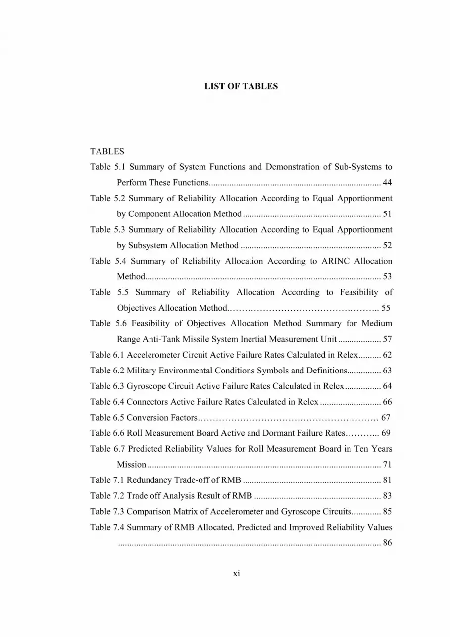
LIST OF TABLES
TABLES
Table 5.1 Summary of System Functions and Demonstration of Sub-Systems to
Perform These Functions............................................................................ 44
Table 5.2 Summary of Reliability Allocation According to Equal Apportionment
by Component Allocation Method ............................................................. 51
Table 5.3 Summary of Reliability Allocation According to Equal Apportionment
by Subsystem Allocation Method .............................................................. 52
Table 5.4 Summary of Reliability Allocation According to ARINC Allocation
Method........................................................................................................ 53
Table 5.5 Summary of Reliability Allocation According to Feasibility of
Objectives Allocation Method.………………………………………….. 55
Table 5.6 Feasibility of Objectives Allocation Method Summary for Medium
Range Anti-Tank Missile System Inertial Measurement Unit ................... 57
Table 6.1 Accelerometer Circuit Active Failure Rates Calculated in Relex.......... 62
Table 6.2 Military Environmental Conditions Symbols and Definitions............... 63
Table 6.3 Gyroscope Circuit Active Failure Rates Calculated in Relex................ 64
Table 6.4 Connectors Active Failure Rates Calculated in Relex ........................... 66
Table 6.5 Conversion Factors…………………………………………………… 67
Table 6.6 Roll Measurement Board Active and Dormant Failure Rates………... 69
Table 6.7 Predicted Reliability Values for Roll Measurement Board in Ten Years
Mission ....................................................................................................... 71
Table 7.1 Redundancy Trade-off of RMB ............................................................. 81
Table 7.2 Trade off Analysis Result of RMB ........................................................ 83
Table 7.3 Comparison Matrix of Accelerometer and Gyroscope Circuits............. 85
Table 7.4 Summary of RMB Allocated, Predicted and Improved Reliability Values
.................................................................................................................... 86

xii
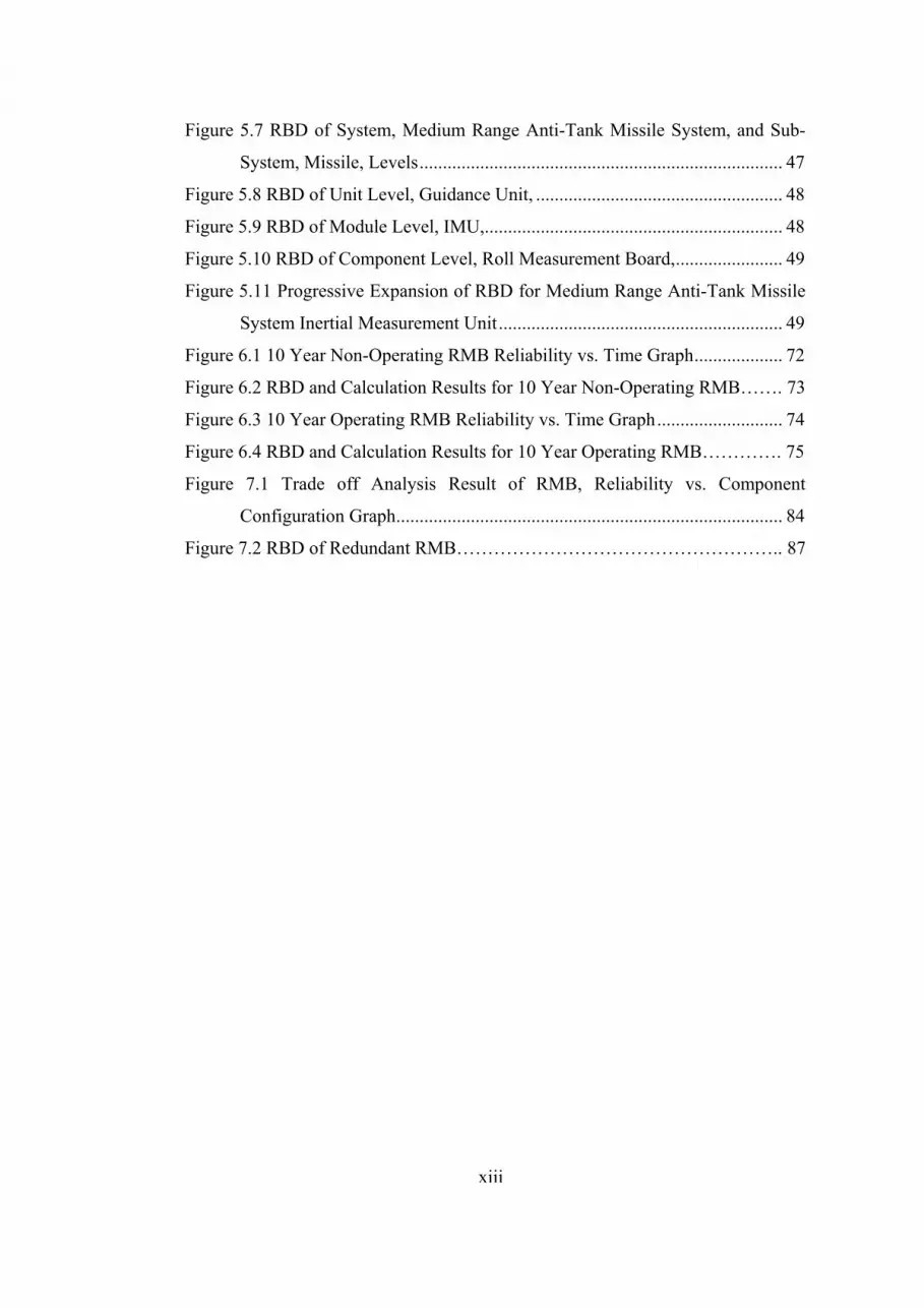
LIST OF FIGURES
FIGURES
Figure 3.1 General Demonstration of m Number of Component Series Model
Configuration [13] ...................................................................................... 13
Figure 3.2 General Demonstration of m Number of Component Parallel Model
Configuration [13] ...................................................................................... 14
Figure 3.3 General Demonstration of m Number of Component Standby Model
Configuration.............................................................................................. 15
Figure 4.1 General Models of Gimbaled and Strapdown IMU Configurations..... 25
Figure 4.2 3-Axis MEMS Accelerometer and Gyroscope Chips........................... 26
Figure 4.3 General Model of a Mechanical Force Feedback Pendulous
Accelerometer ............................................................................................ 27
Figure 4.4 General Model of the Vibrating Beam Accelerometer......................... 28
Figure 4.5 Example Demonstration of Open MEMS Accelerometer .................... 29
Figure 4.6 General Model of Spinning Mass Gyro................................................ 30
Figure 4.7 General Model of Ring Laser Gyro ...................................................... 31
Figure 4.8 General Model of Interferometric Fiber Optic Gyro ............................ 32
Figure 4.9 General Model of Vibratory (Coriolis) Gyro........................................ 32
Figure 4.10 Example Demonstration of Open MEMS Gyroscope ........................ 33
Figure 5.1 Product Tree of the Medium Range Anti-Tank Missile System .......... 36
Figure 5.2 The Anti-Tank Medium Range Missile Main Functions as an FFBD
Format ........................................................................................................ 37
Figure 5.3 Target Acquisition Phase Functions as an FFBD Format…………… 38
Figure 5.4 Firing Sequence Phase Functions as an FFBD Format……………… 40
Figure 5.5 Missile Flight Phase Functions as an FFBD Format………………… 42
Figure 5.6 Target Defection Phase Functions as an FFBD Format ....................... 43
xiii
Figure 5.7 RBD of System, Medium Range Anti-Tank Missile System, and Sub-
System, Missile, Levels.............................................................................. 47
Figure 5.8 RBD of Unit Level, Guidance Unit, ..................................................... 48
Figure 5.9 RBD of Module Level, IMU,................................................................ 48
Figure 5.10 RBD of Component Level, Roll Measurement Board,....................... 49
Figure 5.11 Progressive Expansion of RBD for Medium Range Anti-Tank Missile
System Inertial Measurement Unit............................................................. 49
Figure 6.1 10 Year Non-Operating RMB Reliability vs. Time Graph................... 72
Figure 6.2 RBD and Calculation Results for 10 Year Non-Operating RMB……. 73
Figure 6.3 10 Year Operating RMB Reliability vs. Time Graph........................... 74
Figure 6.4 RBD and Calculation Results for 10 Year Operating RMB…………. 75
Figure 7.1 Trade off Analysis Result of RMB, Reliability vs. Component
Configuration Graph................................................................................... 84
Figure 7.2 RBD of Redundant RMB…………………………………………….. 87

xiv
LIST OF SYMBOLS
Ck Complexity Factor
F(t) Cumulative Distribution Function
f(x) Probability Density Function
Gb Ground, Benign
Gm Ground, Mobile
Mf Missile, Flight
N Quantity of Parts in a Component
RAC Reliability of Accelerometer Circuit
Rc, Ri, Ri(t) Reliability of Component in the System
RC Reliability of Connector
RGC Reliability of Gyroscope Circuit
rik Rating for Feasibility of Objectives Method Criteria
Rk/m Reliability of k out of m Systems
RRMB Reliability of Roll Measurement Board
RSYS Overall System Reliability
S One Line Switch
wi Weighting Factors
wk Sum of the Rated Products
X Number of Redundant System of the Accelerometer Circuit
Y Number of Redundant System of the Gyroscope Circuit

xv
LIST OF ABBREVIATIONS
AC Accelerometer Circuit
CDF Cumulative Distribution Function
COTS Commercial off the Shelf
FFBD Functional Flow Block Diagrams
FOG Fiber Optic Gyroscope
fpmh Failure per million hours
FR Failure Rate
GC Gyroscope Circuit
IMU Inertial Measurement Unit
MB Main Board
MEMS Micro-Electro-Mechanical-Systems
MIL-HDBK Military Handbook
MIL-STD Military Standard
PCB Printed Circuit Board
PDB Power Distribution Board
PMB Pitch Measurement Board
RBD Reliability Block Diagrams
RMB Roll Measurement Board
YMB Yaw Measurement Board

1
CHAPTER 1
INTRODUCTION
1.1. Problem Formulation
Reliability is the probability that a system performs its required functions
under stated conditions for a specific period of time. Time is one of the most
critical elements of reliability and it is generally defined according to system
mission phases, like storage, usage, maintenance. Hence, system reliability may
take different values for different mission phases. Total reliability of the system is
equal to the multiplication of reliability of the mission phases.
High probability of kill, chance of target destruction, is the combination of
essential requirements that drive missile system design for mission reliability.
Values over 95 % are considered to be satisfactory for Mission Reliability in
current missile system designs. Providing a missile system with high mission
reliability requires all of its subsystems to have certain reliability merits. Primary
aim of missiles, like all flying vehicles, is carrying a valuable payload, in this case
it is a warhead, from one position to another. In order to accomplish this mission,
guidance has high importance. Among missile subsystems, one of the most critical
subsystems that has a reduction effect on mission reliability is the Inertial
Measurement Unit (IMU). An IMU produces the angular velocity and acceleration
data for each axis from the inherent gyroscopes and accelerometers. Using this
essential data on board computer determines the missile trajectory. For different
IMUs, selected gyroscopes and accelerometers may vary in terms of performance
characteristics, models and their configurations in IMU. A more accurate IMU
may be designed by changing these sensors’ combination. For example, generally

2
IMU systems have one accelerometer and one gyroscope placed in each axis. IMU
reliability could be improved by using more than one accelerometer and gyroscope
sensors in one axis. Having the right combination of sensors, the IMU that meets
the missile system reliability requirements may be achieved. However, there are
some constraints like cost, mission criticality and size for choosing the right
combination of sensors and trade off analysis has to be carried out very carefully.
For example, to achieve low cost IMU, many sensors which are low sensitivity can
be used instead of using a sensor having high sensitivity and high cost.
In this thesis, IMU reliability model was developed and the corresponding
value of reliability was calculated using MIL-HDBK-217F N2 reliability
prediction methods. Main aim of this thesis is to achieve certain assurance for
reliable functioning of designed IMU system. IMU calculation mistakes like bias,
noise or error drift are not in the scope of this thesis. Furthermore, for the critical
components, such as sensors, redundancy was added to improve IMU reliability, if
it was necessary.
1.2. Scope of the Study
Chapter 2 gives a review of the studies in the literature for reliability
prediction and missile systems reliability.
Chapter 3 consists of the contents; main reliability analysis phases, namely
reliability modeling, reliability allocation, and reliability prediction, which are
explained appropriately regarding the concepts and methods related to this thesis
work.
The aim of usage in missile systems, types, and working principles of
Inertial Measurement Units are briefly explained in Chapter 4.
Designed missile system definition, mission aim, major functions,
component tree and functional flow diagrams are given in Chapter 5. In addition to
those, reliability block diagrams and reliability allocation analysis, which were
done by considering the anti-tank medium range missile system inertial
measurement unit, were given.

3
Chapter 6 introduces reliability prediction analysis of IMU which were
conducted by using Relex Software package program.
Reliability prediction and reliability allocation results are compared in
Chapter 7 and trade-off analysis for the reliability improvement are held.
Conclusion and future work recommendations are given in Chapter 8, the
last chapter of the thesis.

4
CHAPTER 2
LITERATURE SURVEY
2.1. Introduction
Missile systems are designed and produced for a special industry area;
namely military and missile technologies are closely related to national security.
This condition brings limited literature information and limited or confidential
academic studies in missile technology area, especially for reliability topic in
guidance section of a missile. On the other hand, there are several publications
about reliability, such as military standards, books, symposiums, and journals.
2.2. Reliability Standards
Reliability became a subject of study since the World War II, when
complex electronic equipments were used and high failure rates of the equipments
were faced [1]. Since then, various reliability calculation methodologies were
developed and reliability prediction models were formed. These studies are used
worldwide by the help of the military standards and handbooks.
Primary aim of military standards and handbooks is setting universal rules
of a specific topic. For achieving common usage definitions, documentation
procedures, used theories, analytical and test methodologies are defined in the
internationally used documents. Nearly twenty (20) military reliability standards
and handbooks exist in literature and some of them active, some of them cancelled
but still in use for information. Their indexes include all reliability aspects such as,
5
reliability definitions, documentation procedures, monitoring, testing and analysis
methods.
MIL-HDBK-217F and MIL-HDBK-338B are special military standards
about electronic component reliability and they were used in this thesis. In addition
to these, MIL-STD-721C standard was also considered in this thesis.
MIL-HDBK-217F Reliability Prediction of Electronic Equipment [2]:
It is the original reliability prediction handbook that presents a general
origin for reliability predictions. It gives consistent and uniform methods for
estimating electronic equipment and system reliability. It provides two basic
methods for prediction, part stress analysis and parts count. Part stress analysis is
suitable at the end of the detailed design phase when most of the design is
completed and detailed part stress analysis is done which means maximum ratings,
temperature and environmental conditions, etc. are defined. Also, this method
could be appropriate for reliability trade-offs or part selection through the design
improvement phase. Parts count method needs less information compared to parts
stress analysis method. It is proper for early design phase of a system when used
parts category, number, quality level, and application environment of the system
definitions are enough.
MIL-HDBK-338 Electronic Reliability Design Handbook [3]:
It provides guidance, understanding of the concepts, principles, and
methodologies covering all aspects of electronic systems reliability engineering.
Sections in the handbook are composed of; definitions of terms, acronyms,
abbreviations and general statements of reliability, explanation of
reliability/maintainability/availability theory, summary of reliability specification,
allocation, modeling and prediction methods, guidelines for reliability engineering
design, reliability data collection and analysis, demonstration and growth models,
software reliability, systems reliability engineering concepts, production and use
(deployment) of reliability and maintainability, and reliability management
considerations.

6
MIL-STD-721C Definition of Terms for Reliability and Maintainability
[4]:
Aim of this standard is to define reliability and maintainability terms and
definitions for achieving common usage.
2.3. Missile and Sub-Systems Reliability
Micro-Electro-Mechanical Systems (MEMS) technology, which is lately
developed, applications in navigation systems are rapidly increasing. However,
reliability studies for these devices are not sufficient and this brings limited usage
of these devices in high reliability required areas like aerospace industry. Studies
that include IMUs are generally related to its design methodology, calibration
characteristics and methods, and sensor configurations. Especially, there are plenty
of studies in the case of reducing internal errors of IMU. Pasquale [5] defined
reliability testing procedure in vibrating environments for MEMS inertial sensors
and IMUs consist of these sensors. Their sensing performances were evaluated as
combined dynamic excitation test with general sensor calibration and signal
analysis procedures.
At the conceptual design phase of a project, Perera [6] establish reliability
estimation and prediction for MEMS devices by using neural networks. In this
study, MEMS device components attributes and external factors like operating
environment were considered for reliability prediction. For neural network
calculations, attribute data and reliability data of known micro-engines were
collected. As a result, neural networks provide an appropriate predictive
mechanism for MEMS device reliability estimation.
Various redundant configurations of Fiber Optic Gyroscopes (FOG) in
IMUs and the reliability of these different configurations are studied by Zheng and
Wei [7]. First, they defined reliability map of the FOGs used in spacecrafts that are
similar to the reliability block diagrams format. Also, they assume failure rates of
the parts used in the FOG have exponential distribution and this assumption forms

7
the reliability calculation basis, like in this thesis. They examine single axis, four
axes, and six axes redundant configuration of FOG IMU.
Peiravi, whose paper published in the Journal of American Science at 2010
[8], has discussed redundancy and reliability of air to air missile fuze electronics.
In this paper, fuze electronics reliability and incorporate redundancy determined
by failure rate and mean time to failure calculations are done based on MIL-
HDBK-217F. Scope of the methodology in this paper is similar to the related
section of this thesis, however systems used are completely different.
Hoffman [9] used neural networks for estimating 24-month reliability of a
cruise missile by using existing data sources.
For improving the reliability of the bomb fuzing systems used in modern
high-precision guided airborne weapons; Conover [10] eliminated points of failure
by minimizing the mechanical parts used in the fuze and eliminating human factor
through removing the human dependency of the system.
Reliability prediction methods are used in the early phases of the design
rather than reliability testing methods. Bozkaya [11] studied rocket motor
reliability calculation during preliminary design by using probabilistic approaches.
It was seen that, solid rocket motor ballistic performance and casing structure were
the significant parameters affecting the reliability of the rocket motor. Monte Carlo
simulations with the response surface functions method was used to determine
failure probability and rocket motor performance distributions.
8
CHAPTER 3
SHORT OVERVIEW OF RELIABILITY
3.1. Introduction
Reliability is the ability of a system or component to perform a required
function under stated conditions for a specific period of time or number of cycles.
The reliability of the system is related to number of components and parts in the
system, their functional relations to each other and their individual reliabilities
[12]. Reliability prediction is divided into two main prediction models like basic
and mission reliability. Basic reliability prediction estimates the demand for
maintenance and logistic support caused by an item’s unreliability. It is the
measure of ownership cost. Mission reliability prediction estimates the probability
that an item will perform its required functions during the mission. It is the
measure of operational effectiveness [3]. This thesis addresses reliability as
mission reliability. There are various procedures for reliability calculations. The
reliability calculation methodologies are necessarily closely coordinated with
related program activities. In this thesis, reliability modeling and prediction
activities were tailored, appropriate methods were chosen and arranged in proper
order, for the design phases of medium range anti-tank missile system.
Reliability analysis can be divided into three phases such as; modeling,
allocation and prediction.

3.2. Reliability Mathematics
(1) Cumulative Distribution Function (CDF):
It gives the probability of a component failing at time t, eqn. (3.1). In other
words, it is the probability of failure at time t. For continuous random variables,
f(x) is the probability density function that is probability of failure at an instant.
Experimentally, f(x) is the instantaneous slope at time t found on the CDF plot.
t
dxxftF )( , t≥0 (3.1)
Total area under the probability density function between -∞ and +∞ is
equal to unity, 1. Also eqn. (3.1) can be written as eqn. (3.2),
dt
tdFtf
)()( (3.2)
(2) Reliability Function, R(t):
CDF gives probability that a unit will fail before a certain time to t.
t
dxxftFtR )(1)(1)( (3.3)
Reliability is always a non-increasing function of time, because failure
probability is a non-decreasing function, as seen in eqn. (3.3). By putting eqn. (3.2)
in to eqn. (3.3) gives eqn. (3.4),
dt
tdRtf
)()( (3.4)
9

(3) Hazard Rate, λ(t):
It is the rate of failure of units, is not a probability so it can be greater than
1. It is also called failure rate and calculation equation is given by eqn. (3.5).
)(
)()(
tR
tft (3.5)
Eqn. (3.6) gives the most general reliability equation, which is achieved by
substituting eqn. (3.4) into eqn. (3.5), then taking the derivative of both sides and
finally by taking the inverse logarithm.
t
dtt
etR 0
)(
)(
(3.6)
For exponential distribution, probability density function is defined by eqn.
(3.7),
tetf )( (3.7)
From eqn. (3.5) and eqn. (3.7), it is seen that, for an exponential
distribution, failure rate is constant, eqn. (3.8).
)(t (3.8)
Reliability of the component is calculated by using eqn. (3.6), under the
assumption of failure rates of the component are exponentially distributed and
constant, where Ri(t) is the reliability of each one of the elements (in other words,
the probability that the ith element of the system will not fail before time t), λi is
the failure rate of each of the independent elements of the system, and t is
specified time (hour) for reliability calculation, eqn. (3.9).
10

ti
ietR )( (3.9)
In complex systems, for failure rate modeling, commonly exponential
distribution model is used, because of the various forces which can be acting upon
the system and producing failure, like varying environmental conditions, different
part hazard rate functions. Moreover, generally system failure rate oscillates, but
this cyclic movement decreases in time, especially in long-life complex systems,
and approaches a steady state with a constant failure rate regardless of the failure
pattern of individual parts; this is called “approach to a stable state” [3].
3.3. Reliability Modeling
Necessary reliability modeling elements are; system definition, requirement
specification, scenario modeling and Reliability Block Diagrams (RBD). Before
starting any kind of reliability analysis; designed system, aim of system design and
usage of the system, system components and functions should be known. First, the
reliability requirements of the system should be defined. In order to be convenient,
any reliability requirement must be specified quantitatively. Then, environmental
conditions are needed to be defined such as temperature, humidity, vibration in the
transportation, maintenance and operating phases of the designed system. Related
to environmental conditions, mission profiles and time measures should also be
determined. Specifying time is the fundamental step of quantitative description of
reliability. If a system is not operational in all of the life cycle periods, in other
words it has a storage phase, then an expected non-operational time profile, in
addition to the operational time profile should also be defined.
Reliability modeling methods can be listed as; the conventional probability
model, the Boolean Truth table model, the logic diagram model and the simulation
model [3]. In this thesis, conventional probability model was used.
11
12
3.3.1. Reliability Block Diagrams (RBDs)
Reliability block diagrams are prepared for the aim of visual demonstration
of interdependencies between all elements, system working principles and paths
that result in item success. Before drawing a RBD, system mission description,
usage profiles, functions and components should be fully understood. Appropriate
connections such as series, parallel, stand by or combinations of these are used for
the formation of RBD blocks.
Assumptions for RBDs are [3]:
(a) The elements or functions of the items of consideration, which are used
for the evaluation of the reliability with their corresponding individual reliability
value, are associated to the blocks.
(b) The connection lines have no reliability values, they just order the
diagram. The cabling and connectors are included in the diagram as a single block
or induced into part of a block for an element or function.
(c) Failure of any element or function associated with any block in the
diagram will result in failure of the whole item if there are no alternative operation
modes present; ie., redundant units or paths.
(d) Every element or function included into a block in the diagram is
independent regarding the probability of failure from all other blocks.
3.3.1.1. Series Model
In series model, blocks are arranged in a way that they follow each other,
this is the simplest reliability model. In Figure 3.1, m number of components in a
series configuration is shown. For a series model, unit failure results in a system
failure, hence all units must operate normally in order to have a successful system
[13].

Figure 3.1 General Demonstration of m Number of Component Series Model
Configuration [13]
The reliability of series systems, for example shown in Figure 3.1, is
expressed by eqn. (3.10) where RSYS is the overall system reliability and Ri (i=1,
2, 3, …, m) are component reliabilities [13].
mSYS RRRRR 321 (3.10)
3.3.1.2. Parallel Model
In parallel configuration model, system components are operating
simultaneously. This configuration is broadly applied. Figure 3.2 shows the
representation of a parallel configuration model consists of m number of units. In
parallel models at least one normally operating unit results in a successful system
[13].
13

Figure 3.2 General Demonstration of m Number of Component Parallel Model
Configuration [13]
Total system reliability (RSYS) formulation depending on unit reliability
parameters (Ri, i=1, 2, 3, …, m) is given in eqn. (3.11).
mSYS RRRRR 11111 321 (3.11)
3.3.1.3. Combinations of Series and Parallel Model
Especially for a large and complex system, sub-systems can be arranged in
a combination of series and parallel configurations. In these cases, reliability
equations are formed by superposing eqn. (3.10) and eqn. (3.11).
3.3.2. Redundancy
Redundancy is used to improve system reliability. It mainly exists in a
form of parallel system model [3], [13].
3.3.2.1. Parallel System
Same equations and principles used in section 3.2.1.2 are applicable in this
section. If all of the components used in the parallel branches are the same, then
eqn. (3.11) can be simplified into eqn. (3.12), where RSYS is the total system
14
reliability, Rc is the component reliability and m is the number of component used
in parallel redundancy.
15
mCSYS RR 11 (3.12)
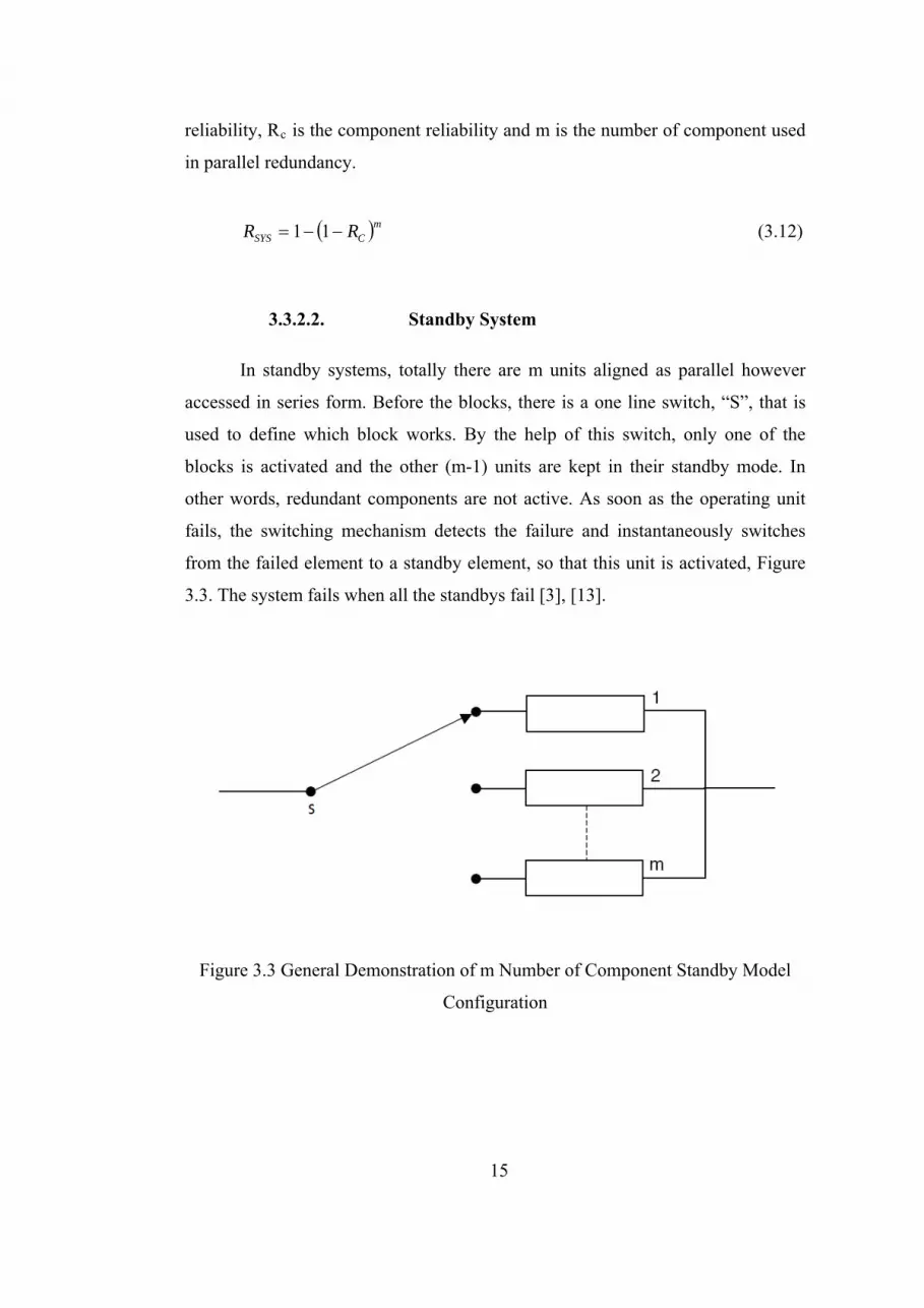
3.3.2.2. Standby System
In standby systems, totally there are m units aligned as parallel however
accessed in series form. Before the blocks, there is a one line switch, “S”, that is
used to define which block works. By the help of this switch, only one of the
blocks is activated and the other (m-1) units are kept in their standby mode. In
other words, redundant components are not active. As soon as the operating unit
fails, the switching mechanism detects the failure and instantaneously switches
from the failed element to a standby element, so that this unit is activated, Figure
3.3. The system fails when all the standbys fail [3], [13].
Figure 3.3 General Demonstration of m Number of Component Standby Model
Configuration
The standby system reliability is given by eqn. (3.13), where the RSYS(t) is
the standby system reliability at time t, λ is the failure rate of the components used,
and m is the total number of units used in the standby system [13].
1
0 !
m
i
it
SYS i
tetR
(3.13)
3.3.2.3. k out of m Systems
This configuration is some sort of a parallel configuration. However,
parallel models need only one of the m units to be operating for the system success
whereas k out of m models need k number of components out of total m number of
components. For independent and identical units, system reliability is calculated
by eqn. (3.14), where the Rk/m is the k out of m system reliability, and Rc is
component reliability [13].
imc
ic
m
kimk RR
i
mR
1/ (3.14)
where,
!)!*(
!
iim
m
i
m
(3.15)
3.4. Reliability Allocation
Previous sections deal with reliability modeling and calculation formulas
related to specific models. These methods are applied in sub-system or in unit
level. However at the beginning of design, reliability requirement is defined at
system level. Sub-system or unit level reliability requirements are not specified
16
17
initially, but those sub-system required reliability values are needed to be specified
to start reliability analysis. In these cases, the designer must assign reliability
objectives of the system to its sub-systems in a well balanced way. For that reason,
special methods for reliability allocation were developed. By using these methods,
designer could be able to determine low level reliability requirements. System
level reliability requirements should be reduced to low level reliability
requirements in a way that low level reliability requirements are proportional to
their functional and physical complexity, mission criticality, and design
limitations. At this point, it is important to choose right allocation methodology. In
literature, there are many allocation methods, namely; Base, Equal Apportionment,
ARINC, Boyd, Agree, Cost, Feasibility of Objectives (Karmiol) [14]. In this
thesis, four different allocation methods were used which are appropriate for new
designed systems.
3.4.1. Equal Apportionment
Equal Apportionment methods are suitable when only knowledge about the
designed system is number and configuration of the sub-systems in the system.
Major weakness of equal apportionment methods is that all components are
viewed as equals, their complexity or the degree of difficulty associated with the
achievement of mission are not accounted. However, in the early stages of design,
equal apportionment methods give reasonable estimations for the definition of low
level desired reliability requirements [15].
3.4.1.1. Equal Apportionment by Component
This method assumes that all sub-systems are in a series configuration and
have the same reliability value. Hence, system reliability is distributed across all
sub-systems equally. If the system consists of n sub-systems, reliability of each
sub-system is equal to the nth root of the system reliability requirement. In other
words, the nth root of the system reliability requirement would be apportioned to
each of the “n” subsystems [3].

Allocated reliability values can be calculated by using eqn. (3.16), where
RSYS is the overall system reliability, Ri (i=1, 2, 3, …) are component reliabilities,
and n is the number of components in the system.
n
iiSYS RR
1
(3.16)
3.4.1.2. Equal Apportionment by Subsystem
Equal apportionment by sub-system is a more complicated method than
equal apportionment by component. This method takes sub-system unit level
complexity into account. In the reliability allocation calculation, sub-system unit
numbers are defined and used as the same way as equal apportionment by
component method. Reliabilities of the units are found by taking their total number
root of the system reliability and sub-system reliability is found by multiplying its
unit reliabilities [15].
3.4.2. ARINC
This technique is based on failure rates of the sub-systems and assumes
series sub-systems configuration with constant failure rates and the initial failure
rates of the sub-systems are known. Initial failure rates can be found from similar
systems, literature or prediction standards [16]. ARINC gives weighting factor to
the sub-systems for the allocation, weighting factors, wi, are calculated by initial
failure rate of the component, λi, divided by initial failure rate of the system, eqn.
(3.17). Then, the allocated failure rates of the components are calculated by
multiplying weighting factors with desired failure rate of the system, λ, eqn. (3.18)
[3].
n
ii
iiw
1
(3.17)
18

ii w (3.18)
3.4.3. Feasibility of Objectives
Feasibility of objectives method was mainly developed for non-repairable
electrical and mechanical systems. In this method, subsystem allocation factors are
defined as functions depending on numerical ratings of system intricacy, state of
the art, performance time, and environmental conditions. These ratings are done by
designers based on their know-how and experience. Voting methods such as the
Delphi technique can also be used by engineer groups in order to determine the
ratings. Method evaluation criteria and definitions are as follows [3];
(1) System Intricacy: Intricacy is evaluated by considering the probable
number of parts or components making up the system and also is judged by the
assembled intricacy of these parts or components. The least intricate system is
rated at 1, and a highly intricate system is rated at 10.
(2) State-of-the-Art: The state of present engineering progress in all fields
is considered. The least developed design or method is a value of 10, and the most
highly developed is assigned a value of 1.
(3) Performance Time: The element that operates for the entire mission
time is rated 10, and the element that operates the least time during the mission is
rated at 1.
(4) Environment: Environmental conditions are also rated from 10 through
1. Elements expected to experience harsh and very severe environments during
their operation are rated as 10, and those expected to encounter the least severe
environments are rated as 1.
Complexity is the normalized sub-system ratings. Complexity of a sub-
system k, , is found by eqn. (3.20) where rkC ik (i= 1, 2, 3, 4) are rating for each of
the four evaluation criteria for each sub-system, wk is multiplication of all ratings
for sub-system k, eqn. (3.19), and N is the number of sub-systems. The allocated
failure rate of the sub-system, λi, is computed by multiplying complexity of a sub-
system with system desired failure rate, λSYS eqn. (3.21) [3]:
19

kkkkk rrrrw 4321 *** (3.19)
N
kk
kkkkk
w
rrrrC
1
4321 (3.20)
SYSki C (3.21)
3.5. Reliability Prediction
In the past, to perform reliability prediction in an early design phase was
considered as a time and money consuming process, whereas nowadays it is
essential to make reliability prediction in the whole design phase of a system.
Reliability prediction helps making better design decisions. In the case of picking
one alternative concept or making choice between used part quality levels
reliability prediction assists designers to make the right choice considering the
system lifetime.
Reliability prediction is a process which is synchronized with system
design. Therefore, prediction techniques have different levels depending upon the
depth of knowledge of the design and the availability of historical data on
equipment and component part reliabilities. System design starts at a conceptual
design phase which defines system mission, system functions, sub-systems
needed, technological feasibility of the sub-systems. Then, it continues with
preliminary and detailed design phases which require more detailed and
quantitative description of sub-systems’ physical and functional properties,
technical drawings, environmental conditions, and stress ratios. Consequently,
reliability prediction techniques should be varying according to the request of
design detail levels.
There are four reliability prediction techniques according to the required
information, which are listed as [3], [12], [17];
20
21
(1) Similar Item Analysis Prediction Method:
It compares analyzed items with similar items, from literature or past
designs, which have known reliability values. Then, known reliability values of the
items are used to estimate probable reliabilities of the analyzed items. In other
words, this method of reliability prediction is based on experience gained from
operational items of similar function. In the usage of this method, one must be
very careful while choosing similar components; similarity necessarily depends on
the degree of equivalence between the items, not simply the generic term used to
describe the items.
(2) Part Count Analysis Prediction Method:
It calculates reliability based on the component type or class and the
number of same type or class components. This method can simply be summarized
as three steps; which of first is to count the number of the same type of
components. In each type of component there is a special calculation function
which defines generic failure rate of the component. Calculating generic failure
rates and multiplying the number of same type components is the second step.
Finally, these products are summed to obtain the total failure rate of the system.
Parts count prediction method is suitable for projects in the preliminary design
phase where the number of the component parts and their generic types (like
resistor, semiconductor, switches etc.) are rationally permanent, except there is not
enough information for calculating stresses acting on the part which is the topic of
the detailed design phase.
(3) Part Stress Analyses Prediction Method:
It forms the basis of the stress analysis. Operational stress levels on the
parts, due to temperature, humidity, vibration, etc., are used for establishing the
failure rate functions of the parts and as expected, for different stress levels, failure
rates of the parts vary. Part stress analysis has four calculation methodologies
according to the data required, namely; stress analysis, sample calculation,
modification for non-exponential failure densities (general case), and non-
operating failure rates. This method is appropriate in the later stages of the design,

22
because it needs details of the system design such as determining stress ratios,
temperature and other application, and environmental data.
(4) Physics-of-Failure Analysis Prediction Method:
It uses complete manufacturing and material properties for calculation of
probability density function and failure mechanism of individual parts. This
reliability prediction method is suitable for the wareout phase of the systems, not
for functional life phase of the systems.
Equations for specific type of parts which were used in this thesis were
given in Appendix A, which are taken from MIL-HDBK-217F. In this thesis,
similar item, part count and part stress analysis methods were all used because of
the variety of design phases of the components.

23
CHAPTER 4
SHORT OVERVIEW OF INERTIAL MEASUREMENT UNIT (IMU)
SYSTEMS
4.1. Introduction
In 1960s, during the ballistic missile programs in the United States, need
for using autonomous navigation systems, which perform navigation using data
produced inside the system (not external data which is sent by an outside user or
system), became crucial. The idea behind this was, if there was no need for
external data for navigation, there would be no data-link between the system and
the surroundings; then the system could not be jammed from outside enemy [18].
This chapter covers the necessity and usage of Inertial Measurement Unit
(IMU), description of its main elements and their working principles.
4.2. Functions of IMU in Missile System
For navigation of missiles the need to known where the target is, which
path should be followed to reach the target, and how to calculate the guidance path
are essential. In the early generation of missile systems these information were
given to the systems externally, by using a wire or a fiber-optic cable. Changing
combat conditions and technology improvements bring the necessity of
autonomous missile systems. For autonomous missile systems, namely fire-and-
forget guided missile systems, mission success depends mostly on the guidance.
Guidance quality is proportional to the accuracy of knowing the location and the
motion of the missile in flight. These requirements brought the necessity of using
24
an Inertial Measurement Unit. IMU is used for determining the position,
orientation and velocity of the system. Most IMUs have three accelerometers and
three single-degree-of-freedom gyroscopes, mounted with orthogonally, to
measure the rotation rates and accelerations [19]. Each accelerometer and
gyroscope measures pitch, roll and yaw rates of the respective axis they
correspond to and then integrates them to find the total change from the initial
position.
All types of accelerometers and gyros exhibit biases, scale factors, cross-
coupling errors, and random noise to certain extent. Most of these errors can be
reduced and corrected by laboratory calibration before usage. On the other hand,
IMU has a weakness of error accumulation. Since the working principle of IMU is
adding new data to the current position data, any error in measurement is
accumulated. This “drift” mainly affects the heading accuracy over time. Another
deficiency of IMU is the need for initial alignment. In other words, it is a dead-
reckoning navigation system and use initial values for obtaining recent data.
In literature, there are mainly two IMU configurations, gimbaled and
strapdown, as shown in Figure 4.1. Gimbaled IMUs are isolated from the platform
rotations by servoed gimbals. They are the first version of IMU’s and not
commonly used today because of their mechanical complexity and cost.
Strapdown IMUs are mounted directly to the platform. They came into the market
in the mid 70’s. They are more reliable, lower cost, and have reduced sizes
compared to gimbaled systems [20].
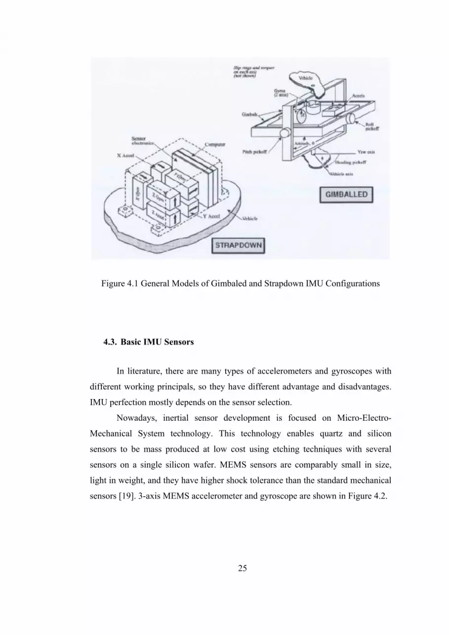
Figure 4.1 General Models of Gimbaled and Strapdown IMU Configurations
4.3. Basic IMU Sensors
In literature, there are many types of accelerometers and gyroscopes with
different working principals, so they have different advantage and disadvantages.
IMU perfection mostly depends on the sensor selection.
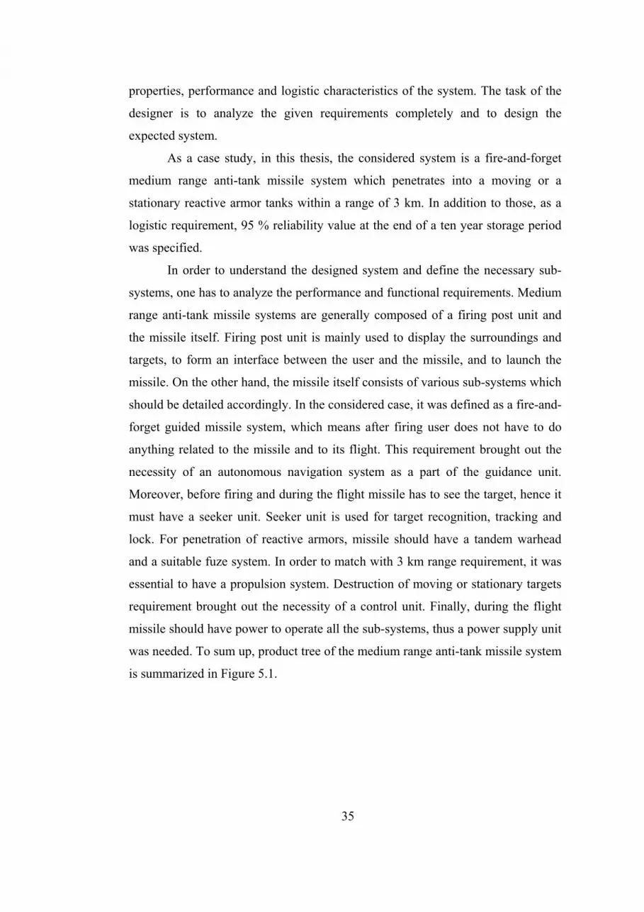
Nowadays, inertial sensor development is focused on Micro-Electro-
Mechanical System technology. This technology enables quartz and silicon
sensors to be mass produced at low cost using etching techniques with several
sensors on a single silicon wafer. MEMS sensors are comparably small in size,
light in weight, and they have higher shock tolerance than the standard mechanical
sensors [19]. 3-axis MEMS accelerometer and gyroscope are shown in Figure 4.2.
25

Figure 4.2 3-Axis MEMS Accelerometer and Gyroscope Chips
4.3.1. Accelerometer
Accelerometer measures the specific force, acceleration, which is generated
by forces acting on a body. Once acceleration of a vehicle is known, velocity and
distance traveled can be determined mathematically; the first integrant of
acceleration is velocity and second integrant is the distance traveled. There are two
types of accelerometers pendulous or vibrating beam and basic principle of both
technologies are the same [19], [20].
4.3.1.1. Pendulous (Mechanical Force Feedback)
Accelerometer
A mechanical force feedback pendulous accelerometers (also called a
closed loop, force rebalanced, or servoed accelerometer) use a close-loop. The
proof mass is attached to the case via a pendulous arm and hinge, forming a
pendulum. The torquer tries to maintain proof mass at a stable position in the
presence of specific force and acceleration. The amount of restoring force, which
is produced by torquer, is determined by the pick-off system which is used to
26

detect departures from the equilibrium position of the proof mass under the
acceleration. Applied acceleration to the system is proportional to the amount of
restoring force [19], [20]. Model of a mechanical force feedback pendulous
accelerometer is given in Figure 4.3.
Figure 4.3 General Model of a Mechanical Force Feedback Pendulous
Accelerometer
4.3.1.2. Vibrating Beam Accelerometer
The Vibrating Beam Accelerometer (also called a Resonant Beam or
Quartz Resonator) also has proof mass and pendulous arm. In contrast to a
mechanical force feedback accelerometer, a vibrating beam accelerometer is an
open-loop device. The beams react to any force applied on the accelerometer case
along the sensitivity axis, by pushing or pulling the proof mass. This causes one of
the beams to resonate under tension and the other under compression. In such
manner, the frequency increases or decreases respectively, Figure 4.4. If the
27

frequency value is measured the specific force applied along the sensitive axis can
be calculated [19], [20].
Figure 4.4 General Model of the Vibrating Beam Accelerometer
4.3.1.3. MEMS Accelerometer
MEMS accelerometers have two different working principles as the
pendulous and vibrating beam accelerometers, whose working principles were
given in preceding parts 4.3.1.1 and 4.3.1.2. First type of accelerometers has been
fabricated in silicon, second type accelerometers has been fabricated from both
quartz and silicon [19], [20]. Open MEMS accelerometer is shown in Figure 4.5.
28

Figure 4.5 Example Demonstration of Open MEMS Accelerometer
4.3.2. Gyroscope
Gyroscopes measure the angular rate of a body. There are three main types
of gyro technology; spinning mass, optical, and vibratory, each of which is based
on a different working mechanism [19], [20].
4.3.2.1. Spinning Mass Gyro
Spinning mass gyros operate with the principle of conservation of angular
momentum, which is the oldest way to measure rotation rate of a body. If a
spinning mass is rotated around an axis (called input axis) orthogonal to its spin
axis there will be a reaction on the third axis (the output axis) orthogonal to both,
Figure 4.6. This reaction can be measured to find the amount of applied rotation
[20]. In the case of closed-loop operation, like a mechanical force feedback
pendulous accelerometer system, the rotating mass is suspended by
electromagnetic torquer. The torque exerted by the torquer is proportional to the
angular rate of the body [19].
29

Figure 4.6 General Model of Spinning Mass Gyro
4.3.2.2. Optical Gyro
Optical gyroscopes work on the principle that, in a given medium, light
travels at a constant speed in an inertial frame. They use the idea of Sagnac effect;
the path length can be changed by rotating the waveguide. If rotation is in the same
direction as the light path, the path length increases. If it is in the opposite
direction, the path length decreases. There are two main types of optical gyros;
Ring Laser Gyro and Interferometric Fiber Optic Gyro [19].
Ring Laser Gyros are used in strapdown inertial navigators since 1975, as a
high-performance technology [18], [19]. Based on the Sagnac effect, if the whole
structure is rotated in one direction, the light beam in the rotated direction will
reach an interaction point later than the beam traveling in the opposite direction.
This time difference will result in shifting of the pattern. The direction and
magnitude of the shift is proportional to the amount of rotation applied to the
structure and is easily measured by counting the moving interference lines, Figure
4.7 [20].
30

Figure 4.7 General Model of Ring Laser Gyro
Interferometric Fiber Optic Gyros (also shortly called fiber optic gyro) are
used since 1985, as a lower cost solution. A broadband light source is divided
using beam splitters into two equal portions that are then sent through a fiber-optic
coil in opposite directions. The beam splitter combines the two beams at the
detector, where the interference between them is observed. When the fiber-optic
coil is rotated about an axis perpendicular to its plane, phase change occurs, Figure
4.8 [18], [19].
31

Figure 4.8 General Model of Interferometric Fiber Optic Gyro
4.3.2.3. Vibratory (Coriolis) Gyro
Vibratory gyros are operating on the Coriolis acceleration of the vibrating
element when the gyro is rotated. When a mass vibrates sinusodially in a rotary
plane a Coriolis force will be generated perpendicular to that plane, which causes a
sinusoidal vibration of that mass along its line of action, Figure 4.9. The angular
rate can be computed by measuring the amplitude of the motion due to the Coriolis
Force [19], [20].
Figure 4.9 General Model of Vibratory (Coriolis) Gyro
32

4.3.2.4. MEMS Gyro
MEMS Gyros are used since 1995, as a small and light solution. All
MEMS gyros operate on the vibratory principle, however they are manufactured
with a different technique. MEMS technology with quartz is giving better
performance than silicone [19], [20].
Figure 4.10 Example Demonstration of Open MEMS Gyroscope
33

34
CHAPTER 5
RELIABILITY MODELING AND ALLOCATION
5.1. Introduction
Reliability analysis consists of three major steps as modeling, allocation,
and prediction. Reliability models help to identify single points of failures, to
evaluate complex configurations and to define series/parallel relationships of all
level units [21]. This chapter of the study focuses on reliability modeling and
allocation. Reliability modeling and allocation was done in the following sequence
[12];
1. Defining the operational requirements, system functions (FFBD)
and configuration (system tree),
2. Constructing Reliability Block Diagrams,
3. Defining the desired reliability values for sub-systems and
components (reliability allocation) to reach a value for the IMU.
Every designed system has to have its requirements. System requirements
define generally expected functions, usage and performance criteria of the system.
RBD helps to understand relationships and hierarchy between sub-systems, units,
and components. After being fully aware of the system, performing reliability
allocation analysis give more accurate results.
5.2. System Requirements and Required Sub-Systems
Every newly developed system has its requirements which were defined
beforehand. These requirements explain expected mission, major physical
35
properties, performance and logistic characteristics of the system. The task of the
designer is to analyze the given requirements completely and to design the
expected system.
As a case study, in this thesis, the considered system is a fire-and-forget
medium range anti-tank missile system which penetrates into a moving or a
stationary reactive armor tanks within a range of 3 km. In addition to those, as a
logistic requirement, 95 % reliability value at the end of a ten year storage period
was specified.
In order to understand the designed system and define the necessary sub-
systems, one has to analyze the performance and functional requirements. Medium
range anti-tank missile systems are generally composed of a firing post unit and
the missile itself. Firing post unit is mainly used to display the surroundings and
targets, to form an interface between the user and the missile, and to launch the
missile. On the other hand, the missile itself consists of various sub-systems which
should be detailed accordingly. In the considered case, it was defined as a fire-and-
forget guided missile system, which means after firing user does not have to do
anything related to the missile and to its flight. This requirement brought out the
necessity of an autonomous navigation system as a part of the guidance unit.
Moreover, before firing and during the flight missile has to see the target, hence it
must have a seeker unit. Seeker unit is used for target recognition, tracking and
lock. For penetration of reactive armors, missile should have a tandem warhead
and a suitable fuze system. In order to match with 3 km range requirement, it was
essential to have a propulsion system. Destruction of moving or stationary targets
requirement brought out the necessity of a control unit. Finally, during the flight
missile should have power to operate all the sub-systems, thus a power supply unit
was needed. To sum up, product tree of the medium range anti-tank missile system
is summarized in Figure 5.1.

Figure 5.1 Product Tree of the Medium Range Anti-Tank Missile System
5.3. Functional Flow Block Diagrams of the System
The aim of Functional Flow Block Diagrams (FFBD) is to show all system
functions necessary for achieving the system success in a chronological order.
FFBDs basically identify the necessary functions in order to achieve the system
success; they do not deal with the equipments used for the actual application.
Functions start after the previous function is completed and they are represented
by blocks. Functions are arranged in a combination of series form, or – and
branches form, and loop form. Also, constraints, input – output signals and data
needed to perform or resulting data of the functions can be shown in FFBDs.
36

FFBDs are important in reliability modeling because they form the basis of the
RBDs.
Based on the system requirements, designed missile system had four
primary functions as;
F1: Acquire Target
F2: Perform Firing Sequence
F3: Perform Flight
F4: Defeat Target
In this thesis, FFBDs were formed by using CORE Enterprise 5.0 [22].
Main functions of the anti-tank medium range missile were modeled in Core by
FFBD format and it is shown in Figure 5.2.
Ref.
1
Acquire Target
2
Perform FiringSequence
3
Perform Flight
4
Defeat TargetRef.
Figure 5.2 The Anti-Tank Medium Range Missile Main Functions as an FFBD
Format
Four main functions of the missile system were detailed in the following
paragraphs.
In the first function, target acquisition phase, seeker starts field search to
detect all targets such as personnel carrier, tank, bus, car, etc. by the help of the
user commands. Then, seeker recognizes the possible targets, meaning tanks, by
circling them on the display. At this point, user chooses the target and sends signal
to the seeker to lock on the chosen target. After target is locked, seeker starts
tracking the target in order not to miss. FFBD of these functions, F1, is given in
Figure 5.3.
37

Fig
ure
5.3
Tar
get A
cqui
siti
on P
hase
Fun
ctio
ns a
s an
FF
BD
For
mat
38

39
In the second function, firing sequence phase, first the missile powers up
all the sub-systems and checks whether all the sub-systems work properly or not.
If one sub-system does not work properly, then the missile cancels the mission. If
all the sub-systems work properly then the missile calculates possible missile flight
path by using mission information which was supplied by the seeker. After flight
path determination, if missile firing signal comes, it fires the propulsion system
and starts the flight, Figure 5.4.

Fig
ure
5.4
Firi
ng S
eque
nce
Pha
se F
unct
ions
as
an F
FB
D F
orm
at
40

41
In the third function, missile flight phase, after leaving launching unit,
missile starts to measure the distance traveled by using IMU system and when safe
distance, which was decided in the design phase by the design authority, is reached
the fuze is activated to set missile ready to explode. During the flight, missile
continuously calculates its position and acceleration, target position and by using
these data (line of sight rate) adjusts the flight path, sends control commands to
control unit, and does required maneuvers. At the same time, while adjusting the
flight path by successive maneuvers, missile continuously measures the remaining
distance to the target. When proper distance is achieved, missile gets out of this
flight phase loop and gets into the last major function, defeat target, Figure 5.5.

Fig
ure
5.5
Mis
sile
Fli
ght P
hase
Fun
ctio
ns a
s an
FF
BD
For
mat
42

Finally in target detection phase, missile hits the target, warhead detonates
and target is destroyed, Figure 5.6.
3
Perform Flight
4.1
Activate WarheadRef.
Target HitSignal
Figure 5.6 Target Defection Phase Functions as an FFBD Format
5.3.1. Sub-System Assignment for Required Functions
It is important to define which sub-system meets which function. Summary
of the missile system major functions and responsible sub-systems of these
functions are given in Table 5.1.
43

44
Table 5.1 Summary of System Functions and Demonstration of Sub-Systems to
Perform These Functions
Function Number &
Name
Performed
By Inputs Outputs
Triggered
By
0 Medium Range Anti
Tank
1 Acquire Target
1.1 Search for Possible
Targets Seeker
1.2 Detect the Target Seeker
1.3 Recognize the
Target Seeker
1.4 Lock the Target Seeker
Target
Locked
Signal
1.5 Track the Target Seeker
2 Perform Firing
Sequence
2.1 Power on all Sub-
Systems
Power
Supply
2.2 Check if all the
Sub-Systems Work
Properly
Guidance

45
Table 5.1 (Continued)
Function Number &
Name
Performed
By Inputs Outputs
Triggered
By
2.3 Calculate Possible
Mission Flight Path Guidance
Mission
Information
Possible
Flight Path
2.4 Fire Missile Propulsion
Motor
Ignition
Signal
Missile
Firing
Signal
2.5 Start Flight Missile
3 Perform Flight
3.1 Activate Fuze Guidance
Fuze
Safe
Distance
Achieved
Signal
3.2 Calculate Missile-
Target Line of Sight Seeker
Line of
Sight
3.3 Measure Missile
Acceleration and
Position
IMU Acceleration
and Position
3.4 Calculate Guidance
Commands Guidance
Acceleration
and Position
Line of
Sight
Guidance
Command
Signal

46
Table 5.1 (Continued)
Function Number &
Name
Performed
By Inputs Outputs
Triggered
By
3.5 Perform Needed
Maneuver Control
Guidance
Command
Signal
3.6 Compute
Remaining Distance to
the Target
Guidance
4 Defeat Target
4.1 Activate Warhead Warhead Target Hit
Signal
5.4. Reliability Block Diagrams
In order to represent the reliability relationships between the system and the
components RBDs are used. While forming the RBDs, physical relationships of
the components do not need to be considered.
The system requirements were taken into consideration to determine
system functions and field experience were used to determine missile sub-system
level product tree in Section 5.2 and Section 5.3. In this part, missile system level
functions were detailed according to IMU; and IMU related RBDs were formed.
Since the aim of this thesis is defining an IMU reliability value, component tree
and modeling of the RBDs were focused on IMU.

Missile systems usually do not have sub-system redundancy because of
limited size (space) and high cost, so each subsystem must function reliably for the
system success. In Figure 5.7 to Figure 5.10, grey boxes define that this sub-
system analyzed one level down. The medium range anti-tank missile system was
divided into two main reliability blocks as missile and firing post unit. The missile,
because of IMU, is the concern of this thesis, thus missile system RBDs were
decomposed to sub-system level by considering main functions of the system
described in Section 5.3, which is seen from Figure 5.7.
Figure 5.7 RBD of System, Medium Range Anti-Tank Missile System, and Sub-
System, Missile, Levels
Main functions of the guidance unit are; checking for firing signal and
sending motor ignition signal to the missile propulsion unit (Electrical Ignition
Board), distributing power to the other sub-systems properly (Power Management
Board), calculating the path to the target and producing control command for
following that path (Guidance Board), supplying position, temperature and
acceleration information (Inertial Measurement Unit), Figure 5.8.
47

Figure 5.8 RBD of Unit Level, Guidance Unit,
Main functions of Inertial Measurement Unit are: producing position and
acceleration information separately on three axes; roll, pitch and yaw, converting
this raw information to digital data recognized by the guidance board. Also,
measuring the temperature is one of the IMU duties. Furthermore each module in
the IMU needs to take power necessarily. RBD of IMU is given in Figure 5.9.
Roll, pitch, and yaw measurement boards have the same physical and functional
properties. The Roll Measurement Board (RMB) was chosen for detailed
reliability analysis and RMB was detailed one level down.
Figure 5.9 RBD of Module Level, IMU,
The duty of the Roll Measurement Board is measuring temperature, linear
and angular acceleration in the X-Frame and sending these measured raw data to
the main board, Figure 5.10.
48

Figure 5.10 RBD of Component Level, Roll Measurement Board,
To sum up, RBDs of the medium range anti-tank missile system formed by
considering the IMU which is summarized in Figure 5.11. The grey boxes define
systems which were examined one-level down.
Figure 5.11 Progressive Expansion of RBD for Medium Range Anti-Tank Missile
System Inertial Measurement Unit
49

50
5.5. Reliability Allocations
In early stages of the system design, the sub-system reliability values are
hard to define. In general, desired system reliability value was defined before the
design. Designer has to distribute desired reliability value towards the sub-system
levels. In these cases distribution of reliability value between the sub-systems was
handled by reliability allocation methods. Reliability allocation deals with the
adjustment of reliability goals for individual subsystems. This is achieved in such a
way that a specified reliability goal for the main system is reached.
In this part, guided missile reliability allocation was hold and required IMU
reliability value was defined.
In this thesis, in order to calculate low-level sub-system desired reliability
value, four common reliability allocation methods, which were previously
explained in Section 3.3, were used to get all the possible desired reliability values
of IMU system needed.
Equal Apportionment by Component method assumes all the sub-systems
have the same priority no matter how complicated design that sub-system requires,
as mentioned in Section 3.3.1.1. Therefore, the desired reliability of the sub-
systems were found by taking the nth root of the desired system reliability, Table
5.2, where n is the total number of sub-systems. In this case the value of n is 7.

51
Table 5.2 Summary of Reliability Allocation According to Equal Apportionment
by Component Allocation Method
Allocated Reliability
Missile 0.95
Seeker 0.9927
Guidance 0.9927
Power Supply 0.9927
Warhead 0.9927
Fuze 0.9927
Propulsion 0.9927
Control 0.9927
Equal Apportionment by Subsystem method takes into account that sub-
system reliabilities were proportional to their unit numbers. It assumes unit level
system numbers express complexity level of a sub-system, Table 5.3. For example,
seeker was composed of 7 units, whereas guidance had combined number of units
of 4 and their reliability values were distributed proportional to these numbers, any
increment in unit level number leads to a decay in desired reliability value.

52
Table 5.3 Summary of Reliability Allocation According to Equal Apportionment
by Subsystem Allocation Method
Unit Number Allocated Reliability
Missile 0.9500
Seeker 7 0.9888
Guidance 4 0.9936
Power Supply 2 0.9968
Warhead 5 0.9920
Fuze 4 0.9936
Propulsion 5 0.9920
Control 5 0.9920
ARINC method distributes sub-system failure rates for their weighting
factors. In order to be able to use ARINC method one needs to have initial
reliability values, in other words failure rates. In this thesis general literature
values of missile systems were used and analysis was conducted based on these
values [23]. The results are shown in Table 5.4.

53
Table 5.4 Summary of Reliability Allocation According to ARINC Allocation
Method
Fleeman
Reliability
Values
Predicted
Failure
Rate (λ)
Weighting
Factor
Allocated
Failure
Rate (λ)
Allocated
Reliability
Values
Missile 0.9500
Seeker 0.9850 2.2491E-05 0.2506 1.9128E-05 0.9872
Guidance 0.9930 1.0453E-05 0.1165 8.8903E-06 0.9940
Power
Supply
0.9950 7.4591E-06 0.0831 6.3438E-06 0.9957
Warhead 0.9950 7.4591E-06 0.0831 6.3438E-06 0.9957
Fuze 0.9870 1.9472E-05 0.2170 1.6560E-05 0.9889
Propulsion 0.9950 7.4591E-06 0.0831 6.3438E-06 0.9957
Control 0.9900 1.4956E-05 0.1666 1.2720E-05 0.9915
Feasibility of Objectives method includes four rating category; namely
system intricacy, state-of-the-art, time, and environment. Weighting of the sub-
systems were done by using the historical data obtained by experienced designers
for these categories. Category definitions were given in Section 3.3.3. When the
system intricacy is taken into consideration, seeker sub-system has the highest
rating because of its complex physical model and high number of parts used in the
sub-system. Guidance unit has average complexity, thus it takes a rating of 5.
State-of-the-art category shows how high developed the engineering process is.
Warhead sub-system has the highest rating for this category. Further, guidance unit

54
has average rating. For performance time category, guidance unit has the highest
rating because of its mission requirement. This unit has to be necessarily
operational for every power up of the missile. Environment category ratings were
nearly the same for every sub-system except the seeker and the control units which
were placed on the outer surface of the missile. Overall designer ratings and
allocated reliability values are given in Table 5.5.

Tab
le 5
.5 S
umm
ary
of R
elia
bili
ty A
lloc
atio
n A
ccor
ding
to F
easi
bili
ty o
f O
bjec
tive
s A
lloc
atio
n M
etho
d
All
ocat
ed
Rel
iab
ilit
y
0.97
5839
0.99
2446
0.99
7819
0.99
8364
0.99
6367
0.99
3470
0.99
4773
All
ocat
ed
FR
(λ)
2.79
01E
-07
8.64
98E
-08
2.49
11E
-08
1.86
83E
-08
4.15
19E
-08
7.47
34E
-08
5.97
87E
-08
Com
ple
xity
0.47
6821
0.14
7824
0.04
2573
0.03
1930
0.07
0956
0.12
7720
0.10
2176
En
viro
nm
ent
8 5 5 5 5 6 8
Tim
e
8 10
6 1 4 6 6
Sta
te-o
f-
the-
Art
7 5 4 9 6 5 3
Sys
tem
Intr
icac
y
9 5 3 6 5 6 6
See
ker
Gui
danc
e U
nit
Pow
er S
uppl
y
War
head
Fuz
e
Pro
puls
ion
Con
trol
55

56
5.6. Discussion
Among the reliability allocation methods most detailed and appropriate one
for this thesis was the Feasibility of Objectives method. This method enables
designer to make comparison between components according to their mission
time, complexity, importance of technology and the environment. Feasibility of
Objectives allocation method was chosen for missile sub-system reliability value
calculation. The rest of the units, modules and components allocated reliability
values were also calculated by using the same method.
To sum up, allocated reliability values for all missile parts related to IMU
were calculated by using the Feasibility of Objectives method. Designers gave the
rating of the sub-systems/units/modules/components by using their know-how for
four specified categories. These ratings for each sub-system are multiplied together
to give an overall rating and then they were normalized to give complexity for the
sub-system, as previously explained in section 3.3.3. As a result, the desired
allocated reliability value for IMU unit was found as 0.996460, which could be
understood form Table 5.6. In the component tree of the IMU system, roll-pitch-
yaw measurement boards have the same parts and properties. Hence, to determine
one of the Printed Circuit Boards (PCBs) allocated reliability value gives failure
rate of all the others.

Table 5.6 Feasibility of Objectives Allocation Method Summary for Medium
Range Anti-Tank Missile System Inertial Measurement Unit
Missile Sub-system LevelSystem
Intricacy State-of-the-Art
Time Environment ComplexityAllocated FR
(λ)Allocated Reliability
Seeker 9 7 8 8 0.476821 2.7901E-07 0.975839
Guidance Unit 5 5 10 5 0.147824 8.6498E-08 0.992446
Power Supply 3 4 6 5 0.042573 2.4911E-08 0.997819
Warhead 6 9 1 5 0.031930 1.8683E-08 0.998364
Fuze 5 6 4 5 0.070956 4.1519E-08 0.996367
Propulsion 6 5 6 6 0.127720 7.4734E-08 0.993470
Control 6 3 6 8 0.102176 5.9787E-08 0.994773
System 0.95
Guidance Unit LevelSystem
Intricacy State-of-the-Art
Time Environment ComplexityAllocated FR
(λ)Allocated Reliability
EIB 3 5 3 5 0.046973 4.0630E-09 0.999644
PDB 3 5 7 5 0.109603 9.4804E-09 0.999169
GB 6 6 10 5 0.375783 3.2504E-08 0.997155
IMU 8 8 7 5 0.467641 4.0450E-08 0.996460
IMU Module LevelSystem
Intricacy State-of-the-Art
Time Environment ComplexityAllocated FR
(λ)Allocated Reliability
RMB 8 8 7 5 0.266667 1.0787E-08 0.999055
PMB 8 8 7 5 0.266667 1.0787E-08 0.999055
YMB 8 8 7 5 0.266667 1.0787E-08 0.999055
MB 6 6 7 5 0.150000 6.0675E-09 0.999468
PDB 3 4 7 5 0.050000 2.0225E-09 0.999823
Roll Measurement Board Component LevelSystem
Intricacy State-of-the-Art
Time Environment ComplexityAllocated FR
(λ)Allocated Reliability
AC 7 8 7 5 0.405797 4.3772E-09 0.999616
GC 9 8 7 5 0.521739 5.6278E-09 0.999507
C 2 5 7 5 0.072464 7.8164E-10 0.999931
57

58
CHAPTER 6
RELIABILITY PREDICTION
6.1. Introduction
Reliability prediction is a living process. It starts from the beginning of the
design till the retirement of the system. Reliability prediction should be carried out
at all phases of the design. This allows the designer, whether reliability
improvement needs of the system can be identified at the early stages of the design
and more reliable configuration or parts can be chosen before it is too late. In other
words, reliability related design decisions could be made in time, otherwise system
failure occurs after the assembly of the system and it is hard, time consuming, and
financially expensive to go back and re-design the system. Furthermore, reliability
prediction should be updated when there is a significant change in the item design,
availability of design details, environmental requirements, stress data, failure rate
data, or service use profile.
This chapter of the study summarizes the reliability analysis done by using
similar item, part count, and part stress prediction analysis methods. Suitable
prediction analysis method was chosen for RMB components. Reliability analyses
were conducted by using the Relex Software and MIL-HDBK-217F.
Reliability analysis was held in the following steps below [3];
1. Classification of the parts of the item and the environmental profile,
2. Determination of the prediction model,
3. Characterization of the failure distribution (exponential, weibull, normal,
etc.)
4. Computation of the item reliability.
59
6.2. Reliability Prediction Methodology
Before starting reliability analysis of the IMU, components used in the
IMU and their design considerations should be defined. Roll, Pitch, Yaw
Measurement Boards (respectively RMB, PMB, and YMB), and Power
Distribution Board (PDB) were designed and produced in ROKETSAN Inc., Main
Board (MB) was purchased from Phytec as a COTS (commercial off the shelf)
item. Therefore, Main Board predicted reliability value was given by Phytec and it
has a fixed reliability value, failure rate. For the rest of the PCB’s predicted
reliability value, failure rate, are needed to be calculated. In this section, detailed
reliability prediction of RMB was given, since PMB and YMB were the same as
RMB.
Generally, reliability value is expressed in terms of failure rate, because of
its mission time dependency. The mission time of the components can vary
according to their functions in the system. Calculating the failure rate of a system
is the main purpose of the reliability prediction. Failure rate can be defined as the
rate of occurrence of failures in a specified period of time. Failure rates of RMB,
PMB, YMB, and PDB were modeled and calculated by using Relex Software and
MIL-HDBK-217F Notice 2 parts count and part stress methodology; MB failure
rate value was given by Phytec. In this thesis, MB and PDB predicted reliability
values are assumed to hold for the expected reliability of IMU, which was
calculated by reliability allocation in section 5.5, because of their simple model
compared to roll, pitch and yaw measurement boards. MIL-HDBK-217 is the
original standard for reliability calculation and it includes mathematical reliability
models for electronic components. In this handbook, every specific type of
component has its own calculation model. Main type of component calculation
models used in this thesis are given in Appendix A. Also, each type of component
has different parameter needs like part temperature, humidity, stress, etc. If the
system has a series configuration, summing all the failure rates of the parts gives
the failure rate of the system [24].

60
For calculation of reliability, initially detailed component tree of RMB was
determined, modeled, service used profiles were defined and then parts failure rate
were calculated in Relex by using MIL-HDBK-217F Notice 2 calculation model.
In addition to this, each part of the component was searched in the Relex library,
for the verification of the calculation model and results were achieved.
Relex is a reliability prediction package based on military handbooks (i.e.
MIL-HDBK-217). Its first version was released in 1987 for reliability calculations.
It is dedicated to meet the product reliability goals of companies from a wide range
of industries like aerospace and defense, automotive, industrial equipment,
electronics and high tech, medical devices. It has got component library database
which gives general properties and failure rates of parts. Moreover, Relex
reliability prediction is used to assess product reliability early in the design
process, to identify leading contributors to system failure, to measure the impact of
environment and stress on the system of interest, and quickly perform series of
reliability calculations and trade-off studies.
6.3. Reliability Models and Calculations
RMB reliability prediction was carried out at component level;
accelerometer circuit, gyroscope circuit, and connectors predicted reliability values
were modeled separately.
In reliability prediction analysis of RMB, before starting the calculation,
some assumptions were done, [12]:
- System components were non-repairable,
- System components were in series configuration (failure of one
component will cause failure of the system),
- System components have constant failure rate,
- System components failure rates were independent for each other,
- System components failure rates followed an exponential
distribution,
- System components have 100 % reliability initially.

6.3.1. Accelerometer Circuit Reliability Prediction Model
RMB accelerometer circuit consists of MEMS accelerometer, capacitors,
resistors and some integrated circuit elements. For modeling, it is important to
define design properties of PCB elements like capacitance, resistance, voltage
limits, operating temperature, and temperature limits, etc. Also, element
configurations and quantities are considerably important. Depth of information
about selected parts affects the success of the reliability prediction method. More
detailed information implies more detailed calculation and more accurate
reliability results can be obtained.
Accelerometer parts tree was formed and modeled in Relex Software by
using appropriate reliability prediction methods. Since accelerometer circuit parts
were arranged in a series order as stated in the assumptions in section 6.3, series
model formula was used for the reliability calculation. If eqn. (3.10) was
rearranged based on the assumptions of exponential distribution and constant
failure rate, the formula for accelerometer circuit failure rate will be found as the
summation of its components failure rates, eqn. (6.1).
2151
611
***...*
**...**
RMBACICRMBACICRMBACRRMBACR
RMBACCRMBACCRMBACMEMSAC
(6.1)
After modeling all parts, reliability calculation was performed and the
results are shown in Table 6.1.
61

62
Table 6.1 Accelerometer Circuit Active Failure Rates Calculated in Relex
Part Number Category Quantity
(N)
Active FR (λ)
(in fpmh)
N*FR
Accelerometer
Circuit
5.547027
RMBACMEMS1 Integrated
Circuit
1 2.032000 2.032000
RMBACC1 Capacitor 2 0.031504 0.063008
RMBACTC2,
RMBACTC3
Capacitor 3 0.828546 2.485638
RMBACC4,
RMBACC5,
RMBACC6
Capacitor 3 0.047684 0.143052
RMBACR1,
RMBACR2
Resistor 2 0.056650 0.113300
RMBACR3 Resistor 1 0.188106 0.188106
RMBACR4,
RMBACR5
Resistor 2 0.100080 0.200160
RMBACIC1 Integrated
Circuit
1 0.297350 0.297350
RMBACIC2 Integrated
Circuit
1 0.024412 0.024412

63
Calculated failure rate of accelerometer was found as 5.547027 fpmh.
These failure rates were calculated at 20o C, missile flight environment and by
using MIL-HDBK-217F calculation model in Relex Software.
In reliability calculation standards environmental conditions are
categorized and generalized for common use. Related environmental conditions
for the medium range anti-tank missile system are given in Table 6.2. These
categorized environmental conditions, symbols and descriptions were taken from
MIL-HDBK-338B [3]. In the case of defining calculation environment as a missile
flight environment, calculation model considers environmental severity related to
flight conditions. If ground benign controlled environment was chosen, failure
rates of the parts takes lower values than failure rates of the missile flight
environmental condition. The reason for this is that the ground benign controlled
environment conditions are less harsh than missile flight environmental conditions.
Table 6.2 Military Environmental Conditions Symbols and Definitions
Environment Symbol Nominal Environmental Conditions
Ground, Benign GB Non-mobile, temperature and humidity
controlled environments.
Ground, Mobile GM
Conditions more severe mostly for
vibration and shock. Equipment installed on
wheeled or tracked vehicles.
Missile, Flight MF
Typical conditions of pressure,
vibration and temperature experienced in
atmospheric flight to target.

64
6.3.2. Gyroscope Circuit Reliability Prediction Model
Gyroscope circuit has two functions, one is measuring the temperature
other one is measuring the angular rate (gyro). Because of its complex theory and
calculation methodology the gyroscope circuit has got more components than the
accelerometer circuit.
Similar procedures as used in the accelerometer circuit were applied to the
gyroscope circuit; parts tree was formed, modeled in Relex, temperature,
environment, and calculation model were set same as that of the accelerometer
circuit and the results of the predicted failure rates are shown in Table 6.3.
Table 6.3 Gyroscope Circuit Active Failure Rates Calculated in Relex
Part Number Category Quantity
(N)
Active FR (λ)
(in fpmh)
N * FR
Gyroscope Circuit 9.738372
RMBGCMEMS1 Integrated
Circuit
1 4.578000 4.578000
RMBGCC10,
RMBGCC14,
RMBGCC19,
RMBGCC21
Capacitor 4 0.031504 0.126016
RMBGCTC11,
RMBGCTC12,
RMBGCTC18,
RMBGCTC20
Capacitor 4 0.828546 3.314184
RMBGCC13,
RMBGCC16,
RMBGCC17
Capacitor 3 0.042277 0.126831

65
Table 6.3 (Continued)
Part Number Category Quantity
(N)
Active FR (λ)
(in fpmh)
N * FR
RMBGCC15 Capacitor 1 0.058155 0.058155
RMBGCR2,
RMBGCR4
Resistor 2 0.188106 0.376212
RMBGCR3,
RMBGCR5
Resistor 2 0.100080 0.200160
RMBGCR6,
RMBGCR9
Resistor 2 0.094378 0.188756
RMBGCR8,
RMBGCR10
Resistor 2 0.031563 0.063126
RMBGCR13,
RMBGCR15
Resistor 2 0.031702 0.063404
RMBGCICU3 Integrated
Circuit
2 0.297350 0.594700
RMBGCICU1 Integrated
Circuit
2 0.024412 0.048824
Failure rate of the gyroscope circuit was 9.738372 fpmh at 20oC and
missile fight environment.

66
6.3.3. Connectors Reliability Prediction Model
Roll Measurement Board has got three connectors. One used for the Main
Board connection, and the other two used for yaw and roll measurement boards
connection. Again same methodology is applied and results are shown in Table
6.4. The calculated connector failure rates, λc, were equal to 0.071610 fpmh.
Table 6.4 Connectors Active Failure Rates Calculated in Relex
Part Number Category Quantity
(N)
Active FR (λ)
(in fpmh)
N*FR
Connector 0.071610
RMBC1,
RMBC2
Connector 2 0.023870 0.047740
RMBC3 Connector 1 0.023870 0.023870
6.4. Reliability Conversion Factors
The conversion factor is used to convert one system phase to another. As
an example, by using adjustment factors one can convert passive (non-working,
dormant, non-operating) failure rates to active (working) failure rates or vice versa
for all environmental conditions, like ground, airborne, naval or space. For a rapid
conversion, tables for different quality levels, various environments and
temperatures are presented to make estimates of the effects of the various changes
[21]. In this thesis conversion factors were taken from Relex Software. In order to
determine the storage (passive) failure rate for a part type, the active failure rates
should be multiplied by the conversion factors listed in Table 6.5. If there is no
valid conversion from the active phase to the dormant phase, the failure rate
should be assumed to be equal to the active failure rate [24].

67
Par
t T
ypes
Gro
und
, Act
ive
To
Gro
un
d,
Pas
sive
Air
bor
ne,
A
ctiv
e T
o A
irb
orn
e,
Pas
sive
Air
bor
ne,
Act
ive
To
Gro
un
d, P
assi
ve
Nav
al, A
ctiv
e T
o N
aval
, P
assi
ve
Nav
al, A
ctiv
e T
o G
rou
nd,
P
assi
ve
Sp
ace,
Act
ive
To
Spac
e,
Pas
sive
Spa
ce, A
ctiv
e T
o G
rou
nd
, P
assi
ve
Cap
acit
ors
0.10
0.10
0.03
0.10
0.04
0.20
0.40
Cir
cuit
Bo
ards
0.04
0.02
0.01
0.03
0.01
0.08
0.20
Con
nect
ors
0.00
50.
005
0.00
30.
008
0.00
30.
020.
03
Dio
des
0.04
0.05
0.01
0.04
0.03
0.20
0.80
Inte
grat
ed
Cir
cuits
0.08
0.06
0.04
0.06
0.05
0.10
0.30
Rel
ays
0.20
0.20
0.04
0.30
0.08
0.40
0.90
Res
isto
rs0.
200.
060.
030.
100.
060.
501.
00
Swit
ches
0.40
0.20
0.10
0.40
0.20
0.80
1.00
Tra
nsfo
rmer
s0.
200.
200.
200.
300.
300.
501.
00
Tra
nsis
tors
0.05
0.06
0.02
0.05
0.03
0.20
1.00
Tab
le 6
.5 C
onve
rsio
n Fa
ctor
s
68
In the considered case of this thesis, missile is going to be stored in the
ground storehouses and when missile system will be activated it will perform in
the air, so airborne active to ground passive conversion factors were used.
6.5. Reliability Prediction Results
To sum up, in this section, Roll Measurement Board in the IMU was
defined, modeled and its predicted failure rate was calculated as active failure rates
(FR) in Relex. Following that, using conversion factor, which were taken from
Relex, storage (non-working) FRs were calculated in Microsoft Excel, Table 6.6.
At the beginning of this section, it was mentioned that all measurement PCBs
(Roll, Pitch and Yaw) have the same configuration, so that they have got the same
value for the failure rates.

69
Nam
eP
art
Nu
mb
erC
ateg
ory
Qu
anti
tyN
Act
ive
Fai
lure
R
ate
(λ)
fpm
hN
*λA
irb
one
acti
ve t
o gr
oun
d p
asiv
e C
onve
rsio
n F
acto
r*
Dor
man
t F
ailu
re
Rat
e (λ
) fp
mh
*N
Rol
l Mea
sure
men
t B
oard
15.3
5700
90.
5345
30
Acc
eler
omet
er C
ircu
it5.
5470
270.
1899
48
RM
BA
CM
EM
S1
Inte
rgra
ted
Cir
cuit
12.
0320
002.
0320
000.
0400
000.
0812
80
RM
BA
CC
1C
apac
itor
20.
0315
040.
0630
080.
0300
000.
0018
90
RM
BA
CT
C2,
RM
BA
CT
C3
Cap
acito
r3
0.82
8546
2.48
5638
0.03
0000
0.07
4569
RM
BA
CC
4, R
MB
AC
C5,
RM
BA
CC
6C
apac
itor
30.
0476
840.
1430
520.
0300
000.
0042
92
RM
BA
CR
1, R
MB
AC
R2
Res
isto
r2
0.05
6650
0.11
3300
0.03
0000
0.00
3399
RM
BA
CR
3R
esis
tor
10.
1881
060.
1881
060.
0300
000.
0056
43
RM
BA
CR
4, R
MB
AC
R5
Res
isto
r2
0.10
0080
0.20
0160
0.03
0000
0.00
6005
RM
BA
CIC
1In
terg
rate
d C
ircu
it1
0.29
7350
0.29
7350
0.04
0000
0.01
1894
RM
BA
CIC
2In
terg
rate
d C
ircu
it1
0.02
4412
0.02
4412
0.04
0000
0.00
0976
Gyr
osco
pe
Cir
cuit
9.73
8372
0.34
4366
RM
BG
CM
EM
S1
Inte
rgra
ted
Cir
cuit
14.
5780
004.
5780
000.
0400
000.
1831
20
RM
BG
CC
10, R
MB
GC
C14
, RM
BG
CC
19, R
MB
GC
C21
Cap
acito
r4
0.03
1504
0.12
6016
0.03
0000
0.00
3780
RM
BG
CT
C11
, RM
BG
CT
C12
, RM
BG
CT
C18
, RM
BG
CT
C20
Cap
acito
r4
0.82
8546
3.31
4184
0.03
0000
0.09
9426
RM
BG
CC
13, R
MB
GC
C16
, RM
BG
CC
17C
apac
itor
30.
0422
770.
1268
310.
0300
000.
0038
05
RM
BG
CC
15C
apac
itor
10.
0581
550.
0581
550.
0300
000.
0017
45
RM
BG
CR
2, R
MB
GC
R4
Res
isto
r2
0.18
8106
0.37
6212
0.03
0000
0.01
1286
RM
BG
CR
3, R
MB
GC
R5
Res
isto
r2
0.10
0080
0.20
0160
0.03
0000
0.00
6005
RM
BG
CR
6, R
MB
GC
R9
Res
isto
r2
0.09
4378
0.18
8756
0.03
0000
0.00
5663
RM
BG
CR
8, R
MB
GC
R10
Res
isto
r2
0.03
1563
0.06
3126
0.03
0000
0.00
1894
RM
BG
CR
13, R
MB
GC
R15
Res
isto
r2
0.03
1702
0.06
3404
0.03
0000
0.00
1902
RM
BG
CIC
U3
Inte
rgra
ted
Cir
cuit
20.
2973
500.
5947
000.
0400
000.
0237
88
RM
BG
CIC
U1
Inte
rgra
ted
Cir
cuit
20.
0244
120.
0488
240.
0400
000.
0019
53
Con
nec
tor
0.07
1610
0.00
0215
RM
BC
1, R
MB
C2
Con
nect
or2
0.02
3870
0.04
7740
0.00
3000
0.00
0143
RM
BC
3C
onne
ctor
10.
0238
700.
0238
700.
0030
000.
0000
72
Tab
le 6
.6 R
oll M
easu
rem
ent B
oard
Act
ive
and
Dor
man
t Fai
lure
Rat
es
Mission profile of the anti-tank missile system was defined as; missile kept
in storehouse for maximum of ten years period and then used for combat. So,
mission of the system can be divided in two phases, one is the storage (non-
working) period for a duration of ten years, and the other one is the usage, active,
period for a duration of few minutes.
The mission failure rate is the sum of the failure rates for each phase, given
by eqn. (6.2).
sedormantphaeactivephasmission (6.2)
The equation for computing the failure rate of an active phase is, eqn.
(6.39):
gesepercentamissionphaactiveeactivephas (6.3)
The equation for computing the failure rate of a dormant phase is given by
eqn. (6.4). The active failure rate is computed using the selected active
environment and temperature. The dormant conversion factor is the factor for
converting from the selected active phase to the selected dormant phase [24].
gesepercentamissionphafactorconversionactivesedormantpha (6.4)
In the case of 3 km range anti-tank missiles average flying times are below
30 seconds. When this value was compared to ten year storage period, which is
87660 hour, it was considered to be an insignificant amount of time. Because of
that, active phase of the missile failure rate was not considered in the reliability
calculation. As stated in Section 5.4, accelerometer circuit, gyroscope circuit and
connectors were in a series form. As a result RMB reliability was calculated by
using a series model formula, eqn. (3.10), which is multiplication of all component
70

71
reliabilities, is equal to system reliability. Predicted reliability summary is given in
Table 6.7.
Table 6.7 Predicted Reliability Values for Roll Measurement Board in Ten Years
Mission
Failure Rate (fpmh) Predicted Reliability
Accelerometer Circuit 0.189948 0.983487
Gyroscope Circuit 0.344366 0.970264
Connectors 0.000215 0.999981
Roll Measurement Board 0.534530 0.954224
Reliability versus time graph for non-working storage phase of the missile
system is seen in Figure 6.1. Relex software calculation results and RBD for 10
year non-operating RMB reliability can be seen in Figure 6.2.

Figure 6.1 10 Year Non-Operating RMB Reliability vs. Time Graph
72

73
Fig
ure
6.2
RB
D a
nd C
alcu
lati
on R
esul
ts f
or 1
0 Y
ear
Non
-Ope
rati
ng R
MB
If it was assumed that the missile was working continuously for 10 years in
missile flight environment, reliability change with time graph, Figure 6.3, and
reliability prediction values decay per annum are shown in Figure 6.4.
Figure 6.3 10 Year Operating RMB Reliability vs. Time Graph
74

75
Fig
ure
6.4
RB
D a
nd C
alcu
lati
on R
esul
ts f
or 1
0 Y
ear
Ope
rati
ng R
MB

76
For ten years non-working system reliability model, reliability value
decreases in time linearly and very slowly, as shown in Figure 6.1. This is because
of low failure rate and non-operating assumption. In Figure 6.3, reliability of the
RMB in the working condition decreases exponentially and faster than non-
working condition, which was expected, because of the ageing, working stresses
and fatigue.
77
CHAPTER 7
TRADE STUDY AND RELIABILITY IMPROVEMENT
7.1. Introduction
As it could be understood from Chapter 5 and Chapter 6, expected
reliability and predicted reliability values of the Roll Measurement Board did not
match. Expected reliability value, 0.99905, was higher than the predicted
reliability value, 0.954224, hence RMB predicted reliability value needed to be
improved. There are two approaches for increasing the reliability of the system,
one approach is to increase the reliability of individual components, and other one
is to duplicate certain components. In IMU reliability improvement case of this
project first method is not applicable. In this project, used accelerometers and
gyroscopes contain latest technology and considerably high reliability value. Other
parts used in IMU; like resistors, capacitors, and connectors are commonly used
standard parts. To change these commonly used parts with high technological ones
would affect the reliability values slightly, because of their physical and usage
characteristics. Furthermore, using advance technology circuit elements brings
high cost but slight increase in reliability value and it is not worth it. Second
method, adding redundancy to the system is suitable for the case considered in this
thesis. Redundancy means, existence of two or more parts generally in a way of
parallel arrangement for achieving component function. In this thesis, same
accelerometer and gyroscope circuits added in a form of parallel branches to the
first circuit for increasing the predicted reliability value to reach desired reliability
value.
This chapter contains the study of improving IMU reliability and
evaluation of feasibility of allocated reliability requirements of the IMU. In order
to accomplish this, components of IMU should be carefully inspected for their
usage, design, size, cost, and importance, so that required number of redundancy
component to be wisely chosen.
7.2. Methodology
Redundancy is used to duplicate the items serving the same function to
prevent failure of an entire system upon failure of a single item. By adding
redundancy in the form of a parallel arrangement, the reliability value was
increased, failure rate was decreased. Reason for this was, in parallel systems,
system does not fail until the entire parallel branches fail. In other words, failure of
one sub-system does not mean system failure and all items of the redundant system
are not required for successful operation.
Types of redundancy can be defined as, parallel operating, standby, k-out-
of-n systems configuration, etc.
Adding redundancy initially decreases system failure rate, but after some
point decreasing rate of the FR become less and less so that, it converges to a
maximum number. This number gives the maximum reliability value for the
system that can be achieved by redundancy. After this point adding parallel
branches does not affect system reliability.
For parallel systems if the failure rates are constant and same for all the
components eqn. (3.12) can be rewritten as eqn. (7.1), where Rsys is the reliability
of the system, Rc is the reliability of the components of the system, λc is the failure
rates of the components, n is the number of redundant components used and T is
the mission time.
nTncSYS
ceRR 1111 (7.1)
78
7.3. Redundancy Analysis
RMB criticality and redundancy necessity should be analyzed based on
their mission and physical properties. Among the components of IMU, power
supply unit needs to be single because of its mission requirements. In addition,
main board used in IMU can not have redundancy because of its size, cost and
relatively high reliability value.
In the case of roll measurement board, connectors can not have the
redundancy since it is defining the interface of one PCB (as an example, roll
measurement boards) to the other PCBs (as an example, pitch measurement
boards, yaw measurement boards). Critical components of the Roll Measurement
Board were the accelerometer circuit and the gyroscope circuit. Their physical and
mission characteristics are appropriate for having redundancy.
As given in Chapter 6, Table 6.6, accelerometer and gyroscope circuits
storage phase, non-working, predicted failure rate values were found respectively
as 0.189948 and 0.344366. Their predicted reliability values were calculated at the
end of ten years storage period respectively as 0.983487 and 0.970264.
Reliability value of the roll measurement board was found by using eqn.
(7.2), where RRMB is the reliability of the Roll Measurement Board, RAC, RGC, and
RC are the reliability of the accelerometer circuit, gyroscope circuit and connectors
respectively, X is the number of redundant system of the Accelerometer Circuit, Y
is the number of redundant system of the Gyroscope Circuit.
CY
GCX
ACRMB RRRR 1111 (7.2)
There are some limitations about the X and Y values. They must be an
integer number. Both have an upper limit of 4 because of size and cost limitations
of the RMB. Designed missile system IMU has to be maximum size of 60x60x80
mm. When IMU is modeled by considering size limitations, sizes of all component
and sensors used in IMU, it was seen that maximum allowable number of each
sensor unit was 4. Moreover, to put extra sensors in the design brings sensor cost
79

80
into account. More sensor usage leads to expensive unit and project budget
limitation need to be taken into account. This project budget was allowed to use
upper limit of 4 of the each sensors. Trade off was done under these considerations
and results are given in Table 7.1.
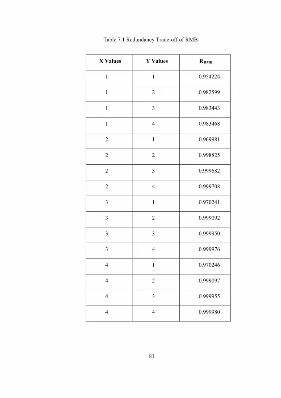
81
Table 7.1 Redundancy Trade-off of RMB
X Values Y Values RRMB
1 1 0.954224
1 2 0.982599
1 3 0.983443
1 4 0.983468
2 1 0.969981
2 2 0.998825
2 3 0.999682
2 4 0.999708
3 1 0.970241
3 2 0.999092
3 3 0.999950
3 4 0.999976
4 1 0.970246
4 2 0.999097
4 3 0.999955
4 4 0.999980

82
7.4. Conclusion
The allocated reliability value for RMB was defined in Chapter 5 as
0.999055. It can be seen in Figure 7.1, adding gyroscope and accelerometer
redundancy affects the system reliability. Reliability contribution of adding
gyroscope circuit was more than adding accelerometer to the board. In Figure 7.1
for the (X, Y) point values, X stands for the number of accelerometer circuit and Y
stands for the number of gyroscope circuit.
In Table 7.2 nearest combination to achieve allocated reliability value were
marked as gray color. Allocated reliability value can be achieved in three different
combinations as 2 AC-3 GC (0.999682), 3 AC-2 GC (0.999092) and 4 AC-2 GC
(0.999097).

83
Table 7.2 Trade off Analysis Result of RMB
X Values Y Values RRMB
1 1 0.954224
1 2 0.982599
1 3 0.983443
1 4 0.983468
2 1 0.969981
2 2 0.998825
2 3 0.999682
2 4 0.999708
3 1 0.970241
3 2 0.999092
3 3 0.999950
3 4 0.999976
4 1 0.970246
4 2 0.999097
4 3 0.999955
4 4 0.999980

Predicted Reliability Trade-off
1,1
4,44,34,23,22,3 3,43,32,42,2
1,41,31,2
4,13,12,1
0,950
0,955
0,960
0,965
0,970
0,975
0,980
0,985
0,990
0,995
1,000
Rel
iab
ilit
y %
Figure 7.1 Trade off Analysis Result of RMB, Reliability vs. Component
Configuration Graph
There was no significant reliability difference between 3 AC and 4 AC.
Therefore, 4 AC-2 GC combination was eliminated. This result also showed that
maximum useful accelerometer circuit redundancy number was 3. Reliability
value was hardly changed after adding third AC to the system.
To determine which circuit has 3 redundancy components it was needed to
look other criteria like cost, mission criticality and size. These three criteria can be
weighted according to their effect on the system as; cost 40%, mission criticality
35% and size 25%. Accelerometer and gyroscope circuits can be rated over 5. In
financial consideration, the gyroscope is slightly expensive than the accelerometer.
For mission importance criteria for both components have the same importance.
Finally, for physical consideration gyroscope (~30 gr) has bigger mass than
accelerometer (~5 gr).
84

85
Table 7.3 Comparison Matrix of Accelerometer and Gyroscope Circuits
Mission
Criticality
Cost Size Total
Weight 0.35 0.40 0.25 1.00
Accelerometer
Circuit
5 5 5 5
Gyroscope
Circuit
5 4 2 3.85
As shown in Table 7.3, adding an accelerometer has got more advantage
than adding a gyroscope. After these considerations, 3 AC-2 GC (0.999092)
combination was selected in the improved model. Summary of RMB allocated,
predicted and improved reliability values are shown in Table 7.4.
Reliability block diagram of the RMB was re-drawn by using Relex
Software and reliability calculation results for ten year period are shown in Figure
7.2.

86
Table 7.4 Summary of RMB Allocated, Predicted and Improved Reliability Values
Allocated
Reliability
Predicted
Reliability
Improved
Reliability
Accelerometer
Circuit 0.999616 0.983487 0.999995
Gyroscope
Circuit 0.999507 0.970264 0.999116
Connectors 0.999931 0.999981 0.999981
Roll Measurement
Board 0.999055 0.954224 0.999092

87
Fig
ure
7.2
RB
D o
f R
edun
dant
RM
B

88
CHAPTER 8
CONCLUSION AND FUTURE WORK
8.1. Conclusion
This thesis discussed the reliability modeling, analysis and improvement of
the Inertial Measurement Unit (IMU) of medium range anti-tank missile system.
Medium range anti-tank missile system desired reliability value was given
as 0.95. Starting from system desired reliability value, allocated reliability value
for medium range anti-tank missile inertial measurement unit was found by using
Feasibility of Objectives method. In addition to that, IMU component tree was
formed, modeled and reliability prediction of the IMU was done by using Relex
Software and MIL-HDBK-217F calculation methods. After all calculations were
complete, allocated reliability and predicted reliability values of the IMU were
compared. Results showed that predicted reliability of the designed IMU was not
good enough to confirm missile system desired reliability. IMU components
configurations, their functional and physical properties were examined for a
possible change and as a result roll-pitch-yaw measurement boards found suitable
for the addition of redundancy. Accelerometer circuit and gyroscope circuit
probable parallel redundancy configurations were determined and predicted
reliabilities were calculated. Best configuration of parallel redundancy was
achieved by using three accelerometer circuits and two gyroscope circuits, 3 AC –
2 GC. Finally, desired reliability of the system was achieved by using this
configuration of IMU.

89
Reliability of a system can be improved by adding redundancy. However,
adding redundancy has disadvantages like increasing cost, size, and complexity of
the system. Design of redundancy, selection of redundant components, redundancy
model and redundant component number should be carefully analyzed.
8.2. Future Work
Although, the analytical calculations were formed by general rules and
include each and every detail of the theory, the actual results could only be reached
by experimental studies.
As a future work, reliability testing needs to be done to verify analytical
reliability prediction results. If there is a difference between test data and analysis
data, using test data will be more adequate. Moreover, based on the test results
redundancy need of the IMU can be reconsidered.
Furthermore, reliability prediction calculations could be conducted for
different characterization of failure distributions like weibull, poisson, and normal.

90
REFERENCES
[1] Bernstein, J. B., Gurfinkel, M., Li, X., Walters, J., Shapira, Y., Talmor, M.,
“Electronic Circuit Reliability Modeling”, Microelectronics Reliability, 46: 1957–
1979, Feburary 2006
[2] MIL-HDBK-217 F Notice 2, “Military Handbook Reliability Prediction of
Electronic Equipment”, Department of Defence, 28 Feburary 1995
[3] MIL-HDBK-338 B, “Military Handbook Electronic Reliability Design
Handbook”, Department of Defence, 1 October 1998
[4] MIL-STD-721 C, “Military Standard Definitions of Terms for Reliability
and Maintainability”, Department of Defence, 12 June 1981
[5] Pasquale, G. D., Somà, A, “Reliability Testing Procedure for MEMS IMUs
Applied to Vibrating Environments”, Sensors, 10: 456-474, January 2010
[6] Perera, J. S. , “Reliability Modeling of Micro-Mechanical Systems Using
Neural Networks”, Ph.D. Thesis, University of Houston, December 2000
[7] Zheng, X., Wei, W., “Reliability Study of Redundant Configuration of IMU
Fiber Optic Gyroscope Inertial Measurement Unit”, AIAA 2009 IEEE Aerospace
Conference, 2009
[8] Peiravi, A., “Redundancy and Reliability of Air to Air Missile Fuze
Electronics”, Journal of American Science, 6(2):147-154, 2010
[9] Hoffman, D. L., “Using Neural Networks For Estimating Cruise Missile
Reliability”, M.Sc. Thesis, Air Force Institute Of Technology, March 2003
[10] Conover, M. R., “Increasing The Reliability Of General Purpose Bomb
Fuzing in Precision Strike Warfare”, M.Sc. Thesis, The University of Tennessee,
December 2006
[11] Bozkaya, K., “A Study On The Reliability Analysis During Preliminary
Design – A Rocket Motor Example”, M.Sc. Thesis, METU, September 2006
91
[12] Relex Software Corporation, “Reliability: A Practitioner’s Guide”, Intellect,
2003
[13] Dhillon, B.S., “Reliability, Quality and Safety for Engineers”, CRC Press
LLC, 2005
[14] Falcone, D., Silvestri, A., Bona, G. D., “Integrated Factors Method for
Reliability Allocation: Application to an Aerospace Prototype Project”, University
of Cassino, Italy
[15] Barbati, S., “Common reliability analysis methods and procedures”,
Reliawind WP 2, Relex, 24 November 2008
[16] Amari, S. V., “New Allocation Methods for Repairable Systems”, AIAA
2009 IEEE Aerospace Conference, 2006
[17] O’CONNER, P. D. T., “Practical Reliability Engineering”, John Wiley &
Sons LTD, 2002
[18] “Low-Cost Navigation Sensors and Integration Technology”, RTO Lecture
Series Supporting Papers, 2010
[19] Groves, P. D., “Principles of GNSS, Inertial, and Multisensor Integrated
Navigation Systems”, Artech House, 2008
[20] “Basic guide to advance navigation”, RTO Nato Set-054/RTG 30, October
2003
[21] Reliability Information Analysis Center, “System Reliability Toolkit, A
Practical Guide for Understanding and Implementing a Program for System
Reliability”, Army Contracting Agency, 2005
[22] CORE Enterprise 5.0 Client, CORE System Definition Guide, Vitech
Corporation, 2004
[23] Fleeman, E. L., “Tactical Missile Design – Integration”, Professional
Development Short Course, 2009
[24] Relex, Team Edition, Help, Parametric Technology Corporation, 2009
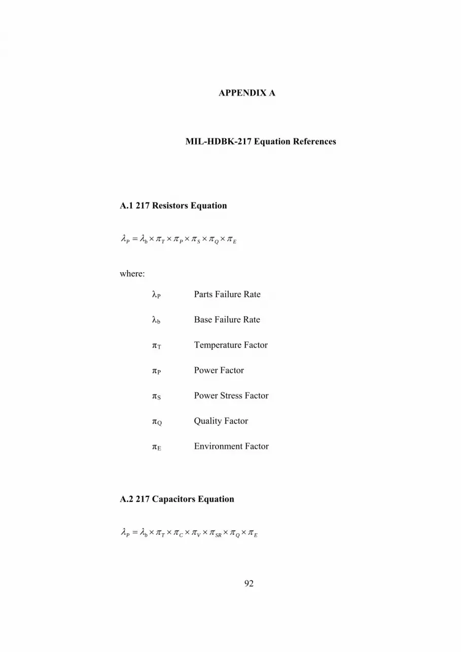
APPENDIX A
MIL-HDBK-217 Equation References
A.1 217 Resistors Equation
EQSPTbP
where:
λP Parts Failure Rate
λb Base Failure Rate
πT Temperature Factor
πP Power Factor
πS Power Stress Factor
πQ Quality Factor
πE Environment Factor
A.2 217 Capacitors Equation
EQSRVCTbP
92

where:
λP Parts Failure Rate
λb Base Failure Rate
πT Temperature Factor
πC Capacitance Factor
πV Voltage Stress Factor
πSR Series Resistance Factor
πQ Quality Factor
πE Environment Factor
A.3 217 Connectors Equation
A.3.1 217 General Connectors Equation
EQKTbP
where:
λP Parts Failure Rate
λb Base Failure Rate
πT Temperature Factor
πK Mating/Unmating Factor
πQ Quality Factor
93

πE Environment Factor
A.3.2 217 Socket Connectors Equation
EQPbP
where:
λP Parts Failure Rate
λb Base Failure Rate
πP Power Factor
πQ Quality Factor
πE Environment Factor
94