cooling curve thermal analyses and oxygen activity - metu

COOLING CURVE THERMAL ANALYSES AND OXYGEN ACTIVITY

ANALYSES FOR THE ESTIMATION OF MICROSTRUCTURAL PROPERTIES

OF NODULAR CAST IRON

A THESIS SUBMITTED TO

THE GRADUATE SCHOOL OF NATURAL AND APPLIED SCIENCES

OF

MIDDLE EAST TECHNICAL UNIVERSITY

BY

CANSIN ÇEHİZ

IN PARTIAL FULFILLMENT OF THE REQUIREMENTS

FOR

THE DEGREE OF MASTER OF SCIENCE

IN

METALLURGICAL AND MATERIALS ENGINEERING

JULY 2019

Approval of the thesis:


ANALYSES FOR THE ESTIMATION OF MICROSTRUCTURAL

PROPERTIES OF NODULAR CAST IRON

submitted by CANSIN ÇEHİZ in partial fulfillment of the requirements for the

degree of Master of Science in Metallurgical and Materials Engineering

Department, Middle East Technical University by,

Prof. Dr. Halil Kalıpçılar

Dean, Graduate School of Natural and Applied Sciences

Prof. Dr. Cemil Hakan Gür

Head of Department, Met. and Mat. Eng.

Prof. Dr. Ali Kalkanlı

Supervisor, Met. and Mat. Eng., METU

Assist. Prof. Dr. Bilge İmer

Co-Supervisor, Met. and Mat. Eng., METU

Examining Committee Members:

Prof. Dr. Vedat Akdeniz

Met. and Mat. Eng., METU

Prof. Dr. Ali Kalkanlı


Assist. Prof. Dr. Bilge İmer


Assist. Prof. Dr. Batur Ercan


Assist. Prof. Dr. Erkan Konca

Met. and Mat. Eng., Atılım University

Date: 26.07.2019

iv

I hereby declare that all information in this document has been obtained and

presented in accordance with academic rules and ethical conduct. I also declare

that, as required by these rules and conduct, I have fully cited and referenced all

material and results that are not original to this work.

Name, Surname:

Signature:

Cansın Çehiz

v

ABSTRACT


ANALYSES FOR THE ESTIMATION OF MICROSTRUCTURAL

PROPERTIES OF NODULAR CAST IRON

Çehiz, Cansın

Master of Science, Metallurgical and Materials Engineering

Supervisor: Prof. Dr. Ali Kalkanlı

Co-Supervisor: Assist. Prof. Dr. Bilge İmer

July 2019, 108 pages

Although nodular cast iron grades have mechanical properties competitive with plain

carbon steel grades, they have advantage in terms of price due to relatively low raw

material and energy costs. Therefore, they are widely used in various industries,

especially in automotive, machinery, piping and wind power industries.

High number of process variables affecting the solidification behavior of nodular cast

iron melt makes it difficult to ensure the resulting microstructure, thus the performance

of nodular cast iron products. Cooling curve thermal analysis and oxygen activity

analysis are two industrially applicable methods which are considered to have a

potential of providing information on the solidification behavior of nodular cast iron

melt.

In this study, chemical composition, cooling curve thermal analysis and oxygen

activity analysis data were collected from the usual production process of Ferromatrix

NV iron foundry in Kortrijk, Belgium. The collected samples were subjected to

metallographic evaluation and tensile test in order to obtain data on the resulting

microstructure and mechanical performance. The alloy EN-GJS-400-18 which is a

ferritic nodular cast iron grade with high ductility, and the alloy EN-GJS-600-10C

vi

which is a solution strengthened ferritic nodular cast iron grade with both high strength

and high ductility were examined. By processing the collected data, conclusions on

the relation of the parameters with each other and their variation between the two alloy

grades and between different inoculant additions were done.

Keywords: Nodular Cast Iron, Cooling Curve, Thermal Analysis, Oxygen Activity

vii

ÖZ

KÜRESEL GRAFİTLİ DÖKME DEMİRDE MİKROYAPISAL

ÖZELLİKLERİN TAHMİNİNE YÖNELİK SOĞUMA EĞRİSİ ISIL

ANALİZLERİ VE OKSİJEN AKTİVİTESİ ANALİZLERİ

Çehiz, Cansın

Yüksek Lisans, Metalurji ve Malzeme Mühendisliği

Tez Danışmanı: Prof. Dr. Ali Kalkanlı

Ortak Tez Danışmanı: Dr. Öğr. Üyesi Bilge İmer

Temmuz 2019, 108 sayfa

Küresel grafitli dökme demirler, yalın karbon çelikleriyle kıyaslanabilir mekanik

özelliklerine karşın, nispeten düşük ham madde ve enerji maliyetleri sayesinde fiyat

avantajı sağlamaktalar. Bu yüzden de, başta otomotiv, makina, tesisat ve rüzgar

enerjisi sanayileri olmak üzere çeşitli alanlarda yaygın olarak kullanılmaktalar.

Küresel grafitli dökme demir ergiyiğinin katılaşma davranımını etkileyen proses

değişkenlerinin çokluğu, sonuçta elde edilecek ürünün mikroyapısını, dolayısıyla da

performansını kontrol altında tutmayı güçleştirmektedir. Soğuma eğrisi ısıl analizi ve

oksijen aktivitesi analizi, küresel grafitli dökme demir ergiyiğinin katılaşma davranımı

üzerine bilgi sağlama potansiyeli bulunan, sanayide kullanıma uygun analiz

yöntemleridir.

Bu çalışmada, Kortrijk, Belçika’da bulunan Ferromatrix NV dökümhanesinin günlük

üretim prosesinden kimyasal bileşim, soğuma eğrisi ısıl analizi ve oksijen aktivitesi

analizi verileri toplanmıştır. Elde edilen numuneler metalografik inceleme ve çekme

testine tabi tutularak sonuçta elde edilen mikroyapı ve mekanik performans üzerine

veriler elde edilmiştir. Ferritik bir küresel grafitli dökme demir olan ve yüksek

süneklik sağlayan EN-GJS-400-18 alaşımı ve katı çözelti sertleşmesiyle

viii

mukavemetlendirilmiş ferritik bir küresel grafitli dökme demir olan ve yüksek

mukavemet ve sünekliği bir arada sağlayan EN-GJS-600-10C alaşımı çalışma

kapsamında incelendi. Elde edilen veriler doğrultusunda, parametrelerin birbirleriyle

ilişkileri, iki alaşım tipi arasında ve farklı aşı ilaveleriyle gösterdikleri değişkenlikler

hakkında çıkarımlar yapıldı.

Anahtar Kelimeler: Küresel Grafitli Dökme Demir, Soğuma Eğrisi, Isıl Analiz,

Oksijen Aktivitesi

ix

To cast iron, the well-known material with lots of unknowns…

x

ACKNOWLEDGEMENTS

The study which is the subject of this thesis was conducted at the Department of

Metallurgical and Materials Engineering of Middle East Technical University, at my

employer Heraeus Electro-Nite Intl. NV and at the foundry Ferromatrix NV.

Firstly, I am grateful to Graduate School of Natural and Applied Sciences and the

Department of Metallurgical and Materials Engineering of Middle East Technical

University for giving me the opportunity to conduct a Master of Science study. I am

more than glad for being able to work under the supervision of Prof. Dr. Ali Kalkanlı,

and I would like to thank to him for all the guidance, supports and encouragement to

the enrichment of this work.

This study would not be present without the continuous improvement seeking

approach of my employer. Thanks to this constructive approach of Heraeus Electro-

Nite Intl. NV providing enormous support both in material aid and in spiritual manner.

I would like to thank to my dear colleagues; Koen Carlier, Frank Seutens, Wolfgang

Baumgart, Danny Van Dooren, Joao Cunha, Francisco Costa Lopes, Monika

Westphalen and Haluk Güldür for their kind supports.

All the field work creating the basis of this study was conducted at the foundry

Ferromatrix NV. Therefore, I would like to thank to them, especially to Frederik Smet

for his interest and collaboration.

My deepest thanks go to my entire family for their regardless, lifelong support,

particularly to my parents Levent and Nevin Çehiz.

xi

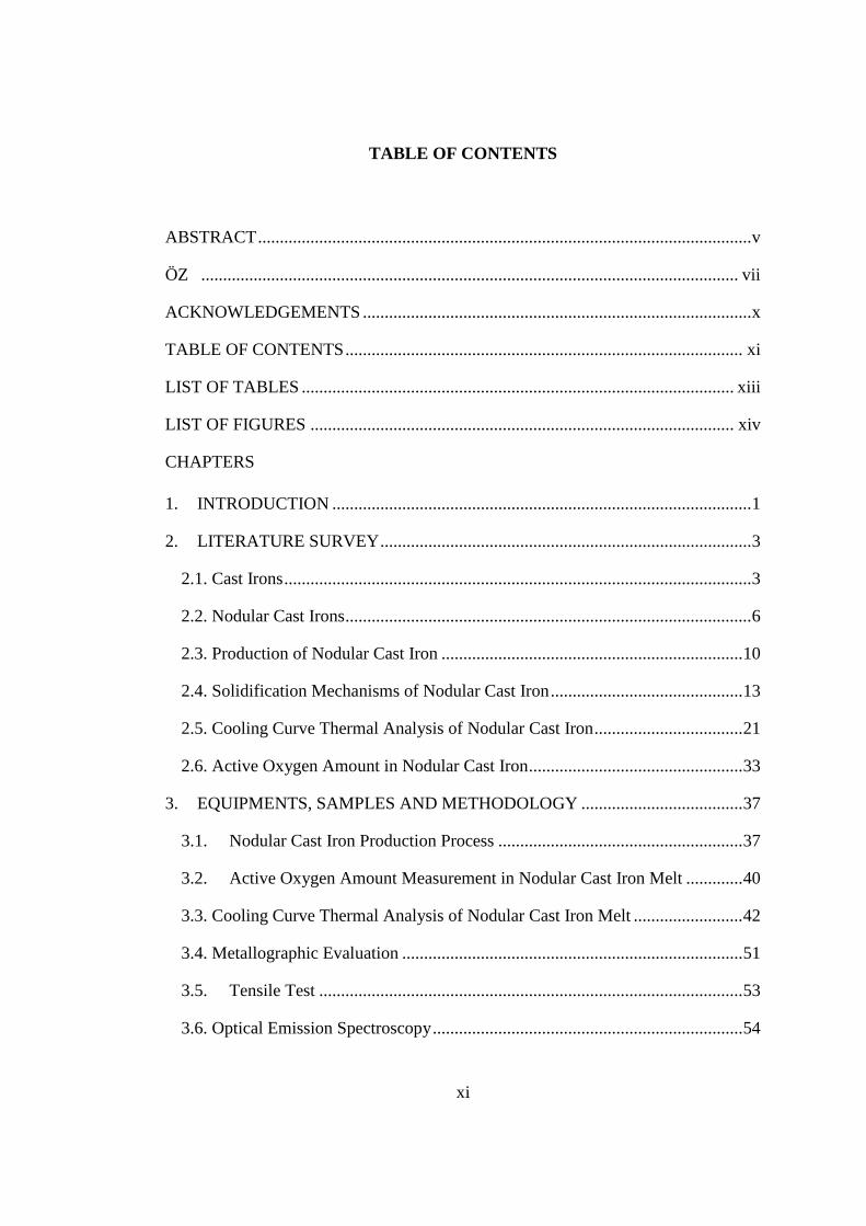
TABLE OF CONTENTS

ABSTRACT ................................................................................................................. v

ÖZ ........................................................................................................................... vii

ACKNOWLEDGEMENTS ......................................................................................... x

TABLE OF CONTENTS ........................................................................................... xi

LIST OF TABLES ................................................................................................... xiii

LIST OF FIGURES ................................................................................................. xiv

CHAPTERS

1. INTRODUCTION ................................................................................................ 1

2. LITERATURE SURVEY ..................................................................................... 3

2.1. Cast Irons ........................................................................................................... 3

2.2. Nodular Cast Irons ............................................................................................. 6

2.3. Production of Nodular Cast Iron ..................................................................... 10

2.4. Solidification Mechanisms of Nodular Cast Iron ............................................ 13

2.5. Cooling Curve Thermal Analysis of Nodular Cast Iron .................................. 21

2.6. Active Oxygen Amount in Nodular Cast Iron ................................................. 33

3. EQUIPMENTS, SAMPLES AND METHODOLOGY ..................................... 37

3.1. Nodular Cast Iron Production Process ........................................................ 37

3.2. Active Oxygen Amount Measurement in Nodular Cast Iron Melt ............. 40

3.3. Cooling Curve Thermal Analysis of Nodular Cast Iron Melt ......................... 42

3.4. Metallographic Evaluation .............................................................................. 51

3.5. Tensile Test ................................................................................................. 53

3.6. Optical Emission Spectroscopy ....................................................................... 54

xii

3.7. Data Correlation .............................................................................................. 54

4. RESULTS AND DISCUSSION ........................................................................ 57

4.1. Chemical Analysis .......................................................................................... 57

4.2. Tensile Test ..................................................................................................... 63

4.3. Cooling Curve Thermal Analysis ................................................................... 65

4.4. Metallographic Image Analysis ...................................................................... 77

4.5. Regression Analysis ........................................................................................ 85

5. CONCLUSIONS .............................................................................................. 101

REFERENCES ........................................................................................................ 105

xiii

LIST OF TABLES

TABLES

Table 2.1. Nodular cast iron grades and their main mechanical properties from tensile

test according to DIN EN1563-3:2012. [10] ................................................................ 9

Table 2.2. Nomenclature and definition of the main points on a nodular cast iron

cooling curve and its first and second derivatives. [27] ............................................. 24

Table 3.1. Chemical composition of the cored wire with Mg master alloy. .............. 39

Table 3.2. Chemical composition of the cored wire with inoculation master alloy... 39

Table 3.3. Description and nomenclature of the cooling curve parameters identified

by MeltControl2020TM. [39] ...................................................................................... 45

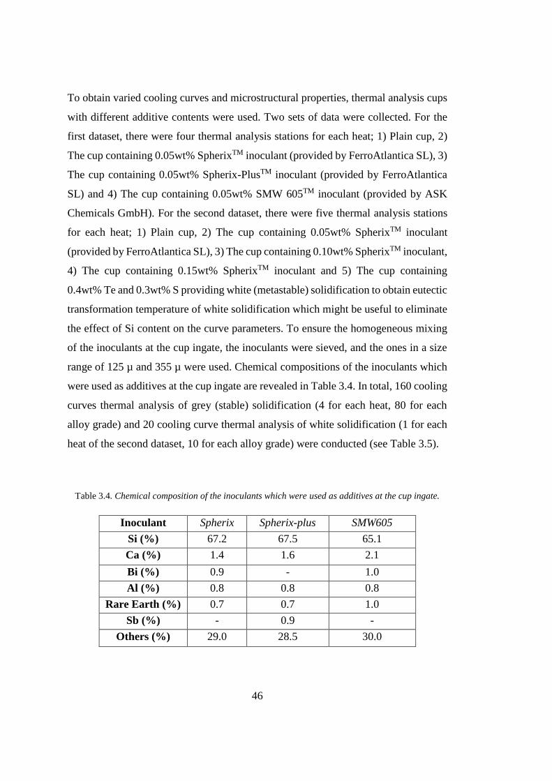
Table 3.4. Chemical composition of the inoculants which were used as additives at the

cup ingate. .................................................................................................................. 46

Table 3.5. List of the cooling curve thermal analysis samples. ................................. 47

Table 4.1. Chemical analysis results obtained by OES and Celox FoundryTM

conducted after the Mg treatment. ............................................................................. 57

Table 4.2. Tensile test results of the specimens obtained from each ladle. ............... 63

Table 4.3. The main results of cooling curve thermal analysis indicating contents of

the analysis cups (Content types; 1-SpherixTM inoculant, 2-Sperix-PlusTM inoculant,

3-SMW605TM inoculant, 4-Te and S). ....................................................................... 65

Table 4.4. The main results of metallographic image analysis indicating contents of

the analysis cups (Content types; 1-SpherixTM inoculant, 2-Sperix-PlusTM inoculant,

3-SMW605TM inoculant, 4-Te and S). ....................................................................... 77

xiv

LIST OF FIGURES

FIGURES

Figure 2.1. Classification of the graphite forms according to the DIN-EN-ISO 9445-

1:2008. [5] .................................................................................................................... 5

Figure 2.2. a) As-polished nodular cast iron microstructure via light microscope; b)

Graphite nodule in etched nodular cast iron microstructure via scanning electron

microscope. [8] ............................................................................................................ 6

Figure 2.3. Number of graphite nodules per unit area in nodular cast iron samples with

different section thickness and inoculation methods. [2] ............................................ 7

Figure 2.4. Schematic representation of the treatment station for Mg cored wire

treatment. [15] ............................................................................................................ 12

Figure 2.5. Fe-C equilibrium phase diagram. [11] .................................................... 14

Figure 2.6. Effect of silicon content on the stable and metastable eutectic

transformation temperatures of Fe-C phase diagram. [2] .......................................... 16

Figure 2.7. Effect of some alloying elements on the stable and metastable eutectic

transformation temperatures of Fe-C phase diagram. [20] ........................................ 17

Figure 2.8. Schematic representation of the grain structure of an ingot casting. [2] . 18

Figure 2.9. a) Schematic representation of the complex, multi-layer sulphide-oxide

inclusion acting as nucleation site for graphite in nodular cast iron; b) A duplex

sulfide-oxide inclusion in nodular cast iron captured via transmission electron

microscope. [23] ........................................................................................................ 19

Figure 2.10. Schematic representation of envelopment of graphite nodules by austenite

phase during solidification of nodular cast iron. [22] ................................................ 20

Figure 2.11. Illustration of the cooling curve of nodular cast iron melt with the first

and second derivatives indicating the main points. [27]............................................ 23

Figure 2.12. Representative cooling curves for the solidification of hypoeutectic,

eutectic and hypereutectic nodular cast iron melts. [29] ........................................... 26

xv

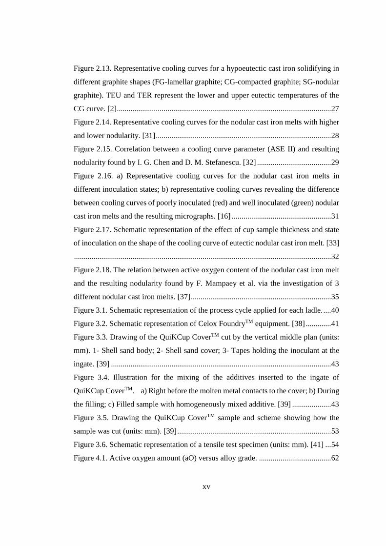
Figure 2.13. Representative cooling curves for a hypoeutectic cast iron solidifying in

different graphite shapes (FG-lamellar graphite; CG-compacted graphite; SG-nodular

graphite). TEU and TER represent the lower and upper eutectic temperatures of the

CG curve. [2] .............................................................................................................. 27

Figure 2.14. Representative cooling curves for the nodular cast iron melts with higher

and lower nodularity. [31] .......................................................................................... 28

Figure 2.15. Correlation between a cooling curve parameter (ASE II) and resulting

nodularity found by I. G. Chen and D. M. Stefanescu. [32] ...................................... 29

Figure 2.16. a) Representative cooling curves for the nodular cast iron melts in

different inoculation states; b) representative cooling curves revealing the difference

between cooling curves of poorly inoculated (red) and well inoculated (green) nodular

cast iron melts and the resulting micrographs. [16] ................................................... 31

Figure 2.17. Schematic representation of the effect of cup sample thickness and state

of inoculation on the shape of the cooling curve of eutectic nodular cast iron melt. [33]

.................................................................................................................................... 32

Figure 2.18. The relation between active oxygen content of the nodular cast iron melt

and the resulting nodularity found by F. Mampaey et al. via the investigation of 3

different nodular cast iron melts. [37] ........................................................................ 35

Figure 3.1. Schematic representation of the process cycle applied for each ladle. .... 40

Figure 3.2. Schematic representation of Celox FoundryTM equipment. [38] ............. 41

Figure 3.3. Drawing of the QuiKCup CoverTM cut by the vertical middle plan (units:

mm). 1- Shell sand body; 2- Shell sand cover; 3- Tapes holding the inoculant at the

ingate. [39] ................................................................................................................. 43

Figure 3.4. Illustration for the mixing of the additives inserted to the ingate of

QuiKCup CoverTM. a) Right before the molten metal contacts to the cover; b) During

the filling; c) Filled sample with homogeneously mixed additive. [39] .................... 43

Figure 3.5. Drawing the QuiKCup CoverTM sample and scheme showing how the

sample was cut (units: mm). [39] ............................................................................... 53

Figure 3.6. Schematic representation of a tensile test specimen (units: mm). [41] ... 54

Figure 4.1. Active oxygen amount (aO) versus alloy grade. ..................................... 62

xvi

Figure 4.2. Liquidus temperature (TL) versus alloy grade. ....................................... 71

Figure 4.3. Upper eutectic temperature (TEmax) versus alloy grade for plain and

inoculated analysis cups separately. .......................................................................... 73

Figure 4.4. Time difference between the end of freezing and lower eutectic (TF_t –

TEmin_t) versus alloy grade. ..................................................................................... 74

Figure 4.5. Liquidus temperature (TL) versus content of the analysis cup. .............. 75

Figure 4.6. Lower eutectic temperature (TEmin) versus content of the analysis cup.

................................................................................................................................... 76

Figure 4.7. Graphite phase area percentage versus alloy grade ................................. 82

Figure 4.8. Graphite nodule count per unit area versus content of the analysis cup . 83

Figure 4.9. Graphite shape nodularity percentage versus content of the analysis cup

................................................................................................................................... 85

Figure 4.10. Ferrite phase area percentage versus graphite nodule count per unit area

graph indicating the alloy grades and linear regression found for the grade EN-GJS-

400-18. ....................................................................................................................... 86

Figure 4.11. Micrographs of some of the etched specimens at 100X magnification. a)

Specimen from cup number 5. b) Specimen from cup number 8. c) Specimen from

cup number 23. d) Specimen from cup number 24. e) Specimen from cup number 35.

f) Specimen from cup number 36. ............................................................................. 88

Figure 4.12. Lower eutectic temperature (TEmin) versus graphite nodule count per

unit area graph for the grade EN-GJS-400-18 indicating content of the analysis cup

and logistic function fit. ............................................................................................. 91

Figure 4.13. Lower eutectic temperature (TEmin) versus graphite nodule count per

unit area graph for the grade EN-GJS-600-10C indicating content of the analysis cup

and logistic function fit. ............................................................................................. 92

Figure 4.14. Lower eutectic temperature calculated by logistic function fit versus

measured lower eutectic temperature graph for the grade EN-GJS-400-18. ............. 93

Figure 4.15. Lower eutectic temperature calculated by logistic function fit versus

measured lower eutectic temperature graph for the grade EN-GJS-600-10C. .......... 94

xvii

Figure 4.16. Micrographs of some of the unetched specimens at 100X magnification.

a) Specimen from cup number 29. b) Specimen from cup number 30. c) Specimen

from cup number 31. d) Specimen from cup number 32. e) Specimen from cup number

93. f) Specimen from cup number 94. g) Specimen from cup number 95. h) Specimen

from cup number 96.

Figure 4.17. Graphite shape nodularity percentage of the specimens from plain cups

versus active oxygen amount (aO) measured in the ladle graph indicating the alloy

grades. ........................................................................................................................ 98

Figure 4.18. Micrographs of some of the unetched specimens at 100X magnification.

a) Specimen from cup number 45. b) Specimen from cup number 57. c) Specimen

from cup number 24. d) Specimen from cup number 108. e) Specimen from cup

number 120. f) Specimen from cup number 112. .................................................... 100

1

CHAPTER 1

1. INTRODUCTION

As the demand for nodular cast iron increases, many foundries take actions to increase

their production capacities in nodular cast iron product range.

When it is compared with lamellar graphite cast iron, nodular cast iron production is

more complex due to the higher number of process parameters that needs to be

controlled and the lower castability.

Especially, to produce ferritic or solution strengthened ferritic nodular cast iron

grades, which are widely used in the applications where ductility is significant, as

many process variables as possible needs to be controlled properly in order achieve

the performance requirements.

To have chemical analysis by using optical emission spectroscopy (OES) and by

combustion analysis (LECO) is quite common in foundries. Although chemical

composition influences the resulting properties, it gives a very limited information on

the solidification behavior which is controlled by various thermodynamic and kinetic

considerations defining the resulting microstructure, thus the performance.

Cooling curve thermal analysis is a method letting us observe temperature versus time

graphs of the samples from the melt while they are cooling and solidifying which can

provide various information on solidification behavior of the melt on the melt-shop

floor in just a few minutes. Therefore, it has a potential to evaluate the melt quality

during the production, and to provide information that can be used to adjust the process

parameters dynamically during the production.

Another useful method is the oxygen activity analysis providing information on the

content of active oxygen, which is the oxygen found in elemental form (not chemically

2

bonded), in the nodular cast iron melt. Since the content of active oxygen has an

important effect on the thermodynamic stability of nodular shape of the graphite

particles found in nodular cast iron structure, it has a potential to provide information

on the resulting structure.

It is known as a fundamental of Materials Engineering that the process defines the

microstructure, and the microstructure defines the performance. Due to the high

number of variables involved in each stage of the process, it is difficult to ensure the

resulting microstructure, therefore the performance of nodular cast iron products.

The aim of this study is to find a scientific method, which is applicable to the industry,

to estimate the resulting microstructural properties of nodular cast iron products by

analyzing the treated nodular cast iron melt. In order to reach this aim, cooling curve

thermal analysis and oxygen activity analysis were applied to the treated nodular cast

iron melts of one ferritic nodular cast iron grade EN-GJS-400-18 and one solution

strengthened ferritic nodular cast iron grade EN-GJS-600-10C. Metallographic

evaluation and tensile tests were also conducted in order to observe the resulting

microstructure and mechanical performance of the collected samples.

3

CHAPTER 2

2. LITERATURE SURVEY

2.1. Cast Irons

Although the earliest iron casting found belongs to the 6th century BC, industrial scale

production of it started at the 18th century in England [1, 2].

At the present day, cast irons are the basic structural materials widely used in many

industries such as automotive, machinery, piping and wind power industries, and they

form 75% of the world production of cast raw products of all metals and alloys [2, 3].

Cast irons are the ferrous alloys containing Carbon (C) more than the solubility limit

in austenite at the eutectic transformation temperature which is 2.14wt% and a

considerable amount of Silicon (Si) [4]. Since the carbon content is higher than the

solubility limit, it forms either graphite with the stable eutectic transformation or

cementite (Fe3C) with the metastable eutectic transformation [2]. Chemical

composition has a significant effect on the microstructure, mechanical properties and

corrosion behavior of cast irons. Therefore, alloying elements such as Copper (Cu),

Manganese (Mn), Tin (Sn), Molybdenum (Mo) and Nickel (Ni) are used to obtain cast

iron products with the desired properties.

With respect to the eutectic transformation type, cast irons can be divided into two

main groups as Grey Cast Iron where stable eutectic transformation resulting carbon

dissociation as graphite occurs and White Cast Iron where metastable transformation

resulting cementite (Fe3C) formation occurs. Their names were originated from the

appearance of their fracture surface. Cementite in White Cast Iron results in brittle

fracture with white and smooth fracture surface where Grey Cast Iron reveals some

deformation prior to fracture, so it has a grey and rougher fracture surface. Therefore,

4

Grey Cast Iron is more favorable in structural applications where White Cast Iron may

result in a catastrophic failure.

Grey Cast Iron is divided into further subgroups. Depending on the shape of graphite

formed during the crystallization, there are three main groups of Grey Cast Iron; 1)

Lamellar Graphite Cast Iron (abbreviated as GJL in EN Standards), 2) Compacted

Graphite Cast Iron (abbreviated as GJV in EN Standards), 3) Nodular Graphite Cast

Iron (abbreviated as GJS in EN Standards) also known as ductile iron [3]. According

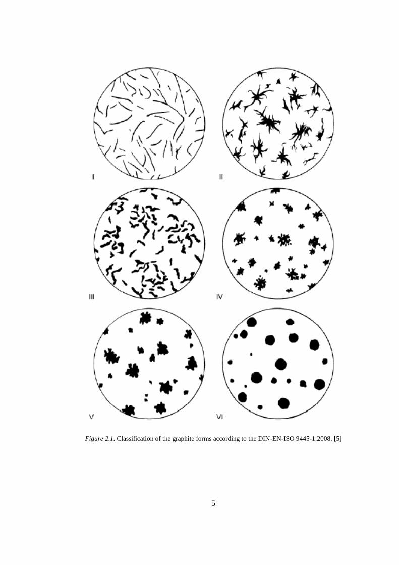
to EN-ISO-9445, there are 6 forms of graphite shape which are revealed in Figure 2.1

[5]. Form I represents the main graphite shape for Lamellar Graphite Cast Iron. Form

III represents the main graphite shape for Compacted Graphite Cast Iron. Form VI

represents the main graphite shape for Nodular Graphite Cast Iron, and the other forms

are the intermediate graphite shapes.

5

Figure 2.1. Classification of the graphite forms according to the DIN-EN-ISO 9445-1:2008. [5]

6

2.2. Nodular Cast Irons

Although industrial production of nodular cast iron has started only 70 years ago, it

represents approximately 25% of the world production of cast raw products of all

metals and alloys [6, 7].

As one can expect from its name, the main characteristic of nodular cast iron is nodule-

shaped graphite particles observed among the matrix (see Figure 2.2) [8].

Figure 2.2. a) As-polished nodular cast iron microstructure via light microscope; b) Graphite nodule

in etched nodular cast iron microstructure via scanning electron microscope. [8]

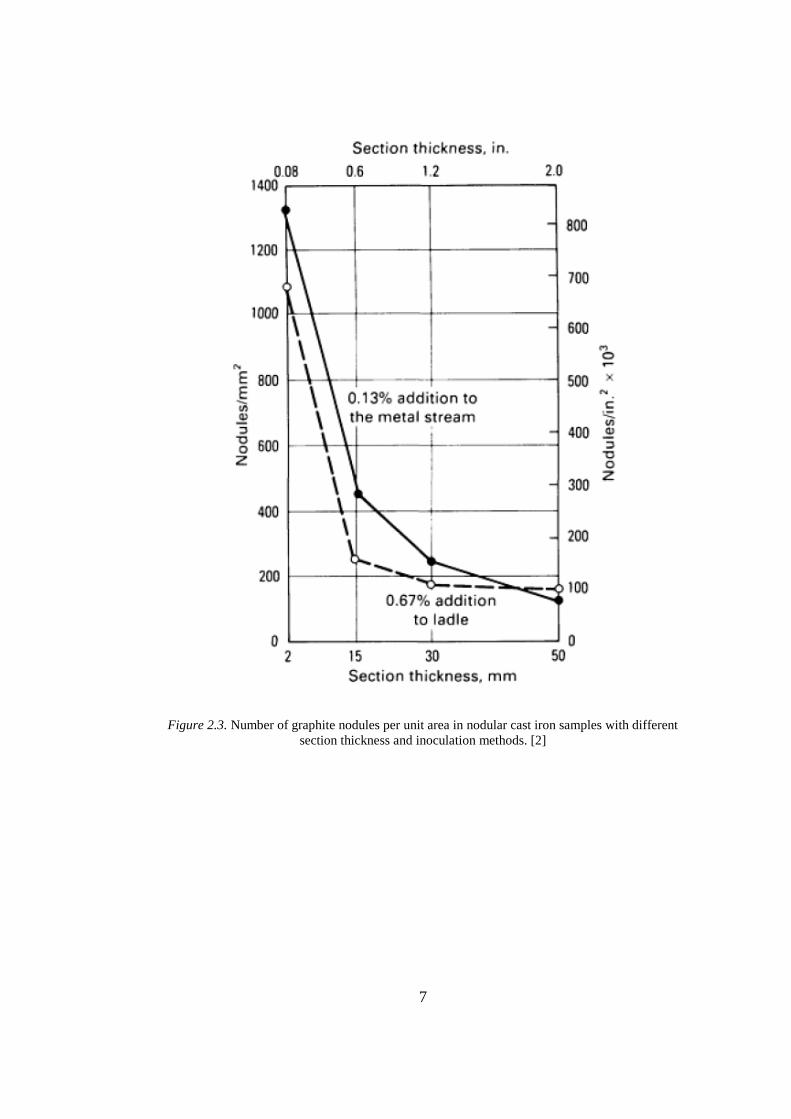
Size and number of the graphite nodules are determined mainly by cooling rate and

amount of heterogeneous nucleation sites [2, 9]. The effect of section thickness, which

defines the cooling rate, and the inoculation method, which affects the amount of

heterogeneous nucleation sites, on the nodule count is represented in Figure 2.3.

7

Figure 2.3. Number of graphite nodules per unit area in nodular cast iron samples with different

section thickness and inoculation methods. [2]

8

Mechanical properties of the nodular cast iron depend on shape, size and number of

graphite nodules, but also content of the matrix [2, 10]. The matrix can be fully ferritic,

fully pearlitic or somewhere in between. The matrix structure is determined mainly by

alloying elements, cooling rate and graphite particle density [2, 8]. Since for some

applications strength is the main concern where it is elongation for some others, there

are different nodular cast iron grades providing different mechanical properties. A list

of those grades according to EN ISO 1563 is revealed in Table 2.1.

9

Table 2.1. Nodular cast iron grades and their main mechanical properties from tensile test according

to DIN EN1563-3:2012. [10]

Material

Designation

Decisive Wall

Thickness

(mm)

Min. Yield

Strength

(MPa)

Min. Tensile

Strength

(MPa)

Min.

Elongation

(%)

EN-GJS-

350-22-LT

t ≤ 30 220 350 22

30 < t ≤ 60 210 330 18

60 < t ≤ 200 200 320 15

EN-GJS-

350-22-RT

t ≤ 30 220 350 22

30 < t ≤ 60 220 330 18

60 < t ≤ 200 210 320 15

EN-GJS-

350-22

t ≤ 30 220 350 22

30 < t ≤ 60 220 330 18

60 < t ≤ 200 210 320 15

EN-GJS-

400-18-LT

t ≤ 30 240 400 18

30 < t ≤ 60 230 380 15

60 < t ≤ 200 220 360 12

EN-GJS-

400-18-RT

t ≤ 30 250 400 18

30 < t ≤ 60 250 390 15

60 < t ≤ 200 240 370 12

EN-GJS-

400-18

t ≤ 30 250 400 18

30 < t ≤ 60 250 390 15

60 < t ≤ 200 240 370 12

EN-GJS-

400-15

t ≤ 30 250 400 15

30 < t ≤ 60 250 390 14

60 < t ≤ 200 240 370 11

EN-GJS-

450-10

t ≤ 30 310 450 10

30 < t ≤ 60 to be agreed between manufacturer and buyer

60 < t ≤ 200

EN-GJS-

500-7

t ≤ 30 320 500 7

30 < t ≤ 60 300 450 7

60 < t ≤ 200 290 420 5

EN-GJS-

600-3

t ≤ 30 370 600 3

30 < t ≤ 60 360 600 2

60 < t ≤ 200 340 550 1

t ≤ 30 420 700 2

10

EN-GJS-

700-2

30 < t ≤ 60 400 700 2

60 < t ≤ 200 380 650 1

EN-GJS-

800-2

t ≤ 30 480 800 2


60 < t ≤ 200

EN-GJS-

900-2

t ≤ 30 600 900 2


60 < t ≤ 200

Although nodular cast iron grades provide a wide range of mechanical properties, their

thermal conductivity varies between 33.5 W/m•K and 36.5 W/m•K (at 100°C) which

is not sufficient for some applications like engine blocks, cylinder heads and brake

discs [2].

2.3. Production of Nodular Cast Iron

Nodular cast iron production process has 3 main metallurgical steps which are melting,

treating and pouring. For each of these steps, there are different methods being used

in the industry, and each step has a significant effect on the resulting properties.

The first step is melting of the raw materials. Melting can be performed by electrical

induction furnaces, electrical arc furnaces or cupola furnaces. Since it provides certain

advantages like ease of operation, flexibility of production, cleaner melt and lower

environmental impact, electrical induction furnace is the most commonly used one.

The charge materials to produce base iron with electrical induction furnaces are

typically pig iron, nodular cast iron returns of the plant to recycle and steel scrap to

lower the carbon content. A special quality pig iron with the requirements; S<0.03%,

P<0.08% and Mn<0.5% needs to be used for nodular cast iron production [11]. In the

case of cupola melting furnace, resulting sulphur content is above the limit due to

nature of the process, and a desulphurization process needs to be conducted typically

by using calcium carbide (CaC2) or Mg addition to the ladle [2]. Desulphurization

11

process needs to be controlled well since at least 0.008% of sulphur content is needed

to create heterogeneous nucleation sites for the graphite particles by inoculation [12].

After melting the raw materials, the alloying additions may be needed to achieve the

aimed chemical composition for the desired alloy grade.

The second step is treating the melt by a high oxygen affinity element, typically Mg.

The aim is to nodularize the graphite shape by decreasing the content of surface-active

elements which are O and S. Tundish cover, wire treatment, sandwich and Georg

Fischer converter are the common methods for Mg treatment. Mg has a boiling point

of 1090oC where the base iron to be treated is generally at above 1400oC, and this

leads to a very aggressive reaction [2]. Therefore, pure Mg usage is not common

unless Georg Fischer converter is the method. Georg Fischer converter has a design

ensuring a safe treatment process even with pure metallic Mg, and it is mostly used in

the plants with cupola furnace for a simultaneous desulfurization and Mg treatment

[2]. For the other methods, Mg ferroalloys with varying Mg contents are commonly

used. The main idea of the methods tundish cover and sandwich is to place the Mg

ferroalloy in a pocket at the bottom of ladle before tapping the base iron from the

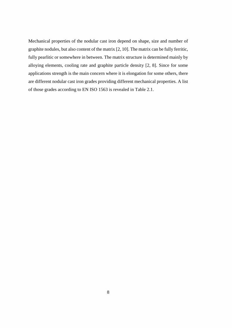
furnace to the ladle. Wire treatment method is also getting more and more popular due

to its highly automatized nature which fits to Industry 4.0 concept. Its main idea is

feeding Mg ferroalloy containing cored wire into the melt by using a wire feeder

machine (see Figure 2.4). Another advantage of wire treatment is the ability of

calculation of the treatment alloy addition ratio accurately. Since the treatment alloy

is fed after the melt is tapped into the ladle, it is possible to measure the exact weight

of the melt and to calculate the addition amount accordingly which is not the case for

the other treatment methods. In terms of Mg yield, wire treatment has a disadvantage

such that it has a Mg yield in range of 40% to 60% which is 60% to 80% for tundish

cover and sandwich methods [13, 14].

12

Figure 2.4. Schematic representation of the treatment station for Mg cored wire treatment. [15]

The last step is pouring the treated melt into the molds. To provide heterogeneous

nucleation sites favoring the graphite nucleation, inoculant alloy particles needs to be

added into the ladle, into the mold or into the stream in between. There are various

types of inoculant with different chemical compositions and particle sizes depending

on the application place. For example, the inoculants containing Ba as active element

have relatively low inoculation effect, but they have a high fading resistance which

makes them good for ladle application where the ones containing Sr have very strong

inoculation effect with very limited fading resistance which makes them good for

stream application [16].

13

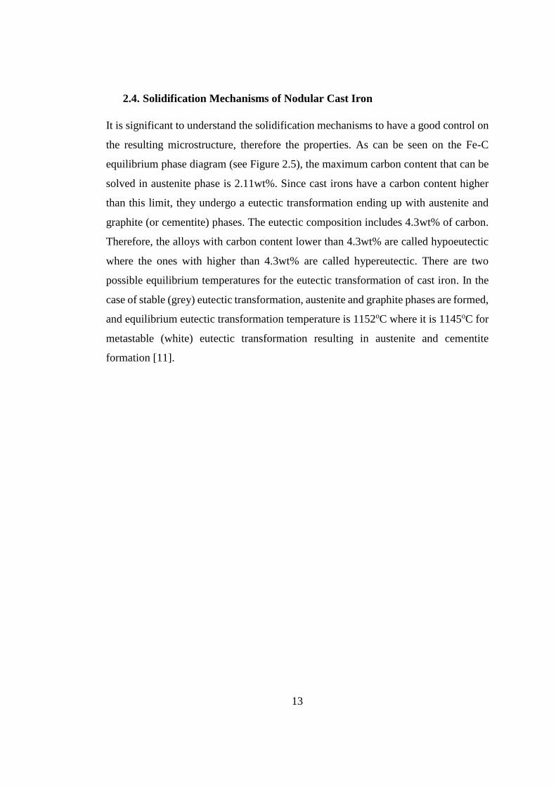
2.4. Solidification Mechanisms of Nodular Cast Iron

It is significant to understand the solidification mechanisms to have a good control on

the resulting microstructure, therefore the properties. As can be seen on the Fe-C

equilibrium phase diagram (see Figure 2.5), the maximum carbon content that can be

solved in austenite phase is 2.11wt%. Since cast irons have a carbon content higher

than this limit, they undergo a eutectic transformation ending up with austenite and

graphite (or cementite) phases. The eutectic composition includes 4.3wt% of carbon.

Therefore, the alloys with carbon content lower than 4.3wt% are called hypoeutectic

where the ones with higher than 4.3wt% are called hypereutectic. There are two

possible equilibrium temperatures for the eutectic transformation of cast iron. In the

case of stable (grey) eutectic transformation, austenite and graphite phases are formed,

and equilibrium eutectic transformation temperature is 1152oC where it is 1145oC for

metastable (white) eutectic transformation resulting in austenite and cementite

formation [11].

14

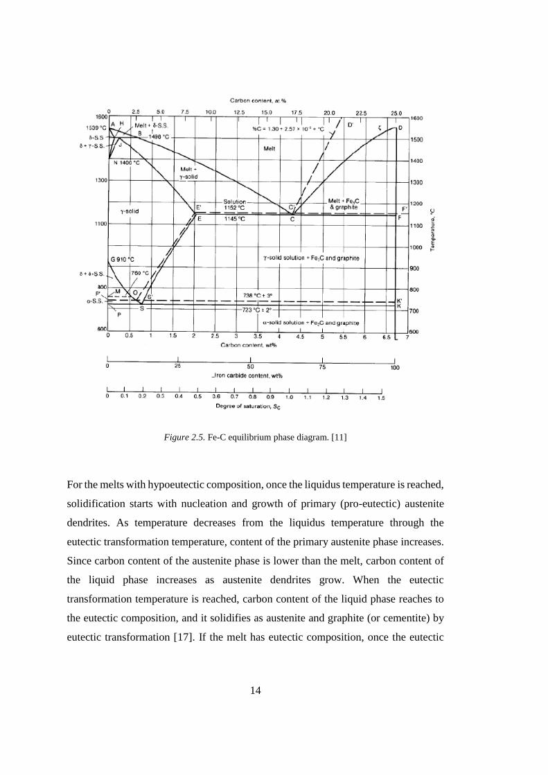
Figure 2.5. Fe-C equilibrium phase diagram. [11]

For the melts with hypoeutectic composition, once the liquidus temperature is reached,

solidification starts with nucleation and growth of primary (pro-eutectic) austenite

dendrites. As temperature decreases from the liquidus temperature through the

eutectic transformation temperature, content of the primary austenite phase increases.

Since carbon content of the austenite phase is lower than the melt, carbon content of

the liquid phase increases as austenite dendrites grow. When the eutectic

transformation temperature is reached, carbon content of the liquid phase reaches to

the eutectic composition, and it solidifies as austenite and graphite (or cementite) by

eutectic transformation [17]. If the melt has eutectic composition, once the eutectic

15

transformation temperature is reached, entire melt solidifies by eutectic

transformation. For the ones with hypereutectic composition, solidification starts at

liquidus temperature as in hypoeutectic but this time with nucleation and growth of

primary graphite instead of austenite. As a result of further temperature decrease,

primary graphite content increases, and carbon content of the liquid phase decreases.

At eutectic transformation temperature, carbon content of the liquid phase becomes

equal to the eutectic composition, and it solidifies by eutectic transformation.

Fe-C equilibrium phase diagram applies for iron carbon binary systems, but cast iron

includes many elements other than iron and carbon. Most of these elements are

commonly in small portions, but the content of silicon is significantly high since it

favors the stable (grey) solidification. This situation requires the use of a ternary Fe-

C-Si phase diagram. It was discovered that increasing silicon content reduces the

carbon content at eutectic point and carbon solubility in austenite phase. Therefore,

with a correction factor applied to the carbon content, Fe-C binary phase diagram can

be used for cast iron alloys. This corrected carbon content replacing the carbon content

on the X-axis of the diagram is called as Carbon Equivalent (C.E.), and it is calculated

by Equation 2.1 [19]. In addition, the empirical formula (Equation 2.2) based on the

effect of carbon, silicon and phosphor contents on Fe-C binary phase diagram was

created by Heraeus Electro-Nite Intl. NV by using the liquidus temperatures obtained

by cooling curve thermal analysis and the chemical analysis results obtained by

combustion (LECO) analysis [18].

Equation 2.1. C.E. [%] = C [%] + (Si [%] + P [%]) / 3

Equation 2.2. C.E.L. [%] = C [%] + (Si [%]) / 4 + (P [%]) / 2

16

Silicon and some other elements have an effect on stable (grey) and metastable (white)

eutectic transformation temperatures (see Figure 2.6 and 2.7). For a cast iron melt to

have a metastable eutectic transformation, it needs to have an undercooling equal to

the difference between stable and metastable eutectic transformation temperatures.

Therefore, the elements increasing this difference by increasing the stable eutectic

temperature and decreasing the metastable one favor the stable (grey) solidification,

and they are called graphitizing elements. Silicon, nickel, cobalt and copper are the

common examples for graphitizing elements. On the other hand, the elements

decreasing the difference between stable and metastable eutectic temperatures by

reducing the stable eutectic temperature and increasing the metastable one favor the

metastable (white) solidification, and they are called carbide formers. Chromium,

titanium and vanadium are the common examples for carbide formers. Although they

give us some idea about the solidification sequence, it is important to remind that

equilibrium phase diagrams are based on thermodynamic calculations, and they apply

at equilibrium conditions which cannot be met in industrial scale.

Figure 2.6. Effect of silicon content on the stable and metastable eutectic transformation temperatures

of Fe-C phase diagram. [2]

17

Figure 2.7. Effect of some alloying elements on the stable and metastable eutectic transformation

temperatures of Fe-C phase diagram. [20]

18

Nucleation of primary (pro-eutectic) austenite occurs heterogeneously on the interface

of some solid particles like oxides and carbides with liquid phase [21]. Then, it is

followed by the growth with a non-planar solidification interface such as columnar or

equiaxed dendritic depending on the required nucleation undercooling and the

magnitude of constitutional undercooling [2, 22]. For a typical ingot casting (see

Figure 2.8), the nucleus formed on the mould wall heterogeneously are likely to have

columnar growth towards the center of mould which is the opposite direction of heat

flow, then their growth might be terminated by the equiaxed grains if the undercooling

needed for the nucleation of equiaxed grains is less than the constitutional

undercooling ahead of the growing columnar grains [2, 22].

Figure 2.8. Schematic representation of the grain structure of an ingot casting. [2]

19

The graphite phase also nucleates heterogeneously on the interface of some solid

particles with liquid phase, since it is more feasible in terms of energy [2]. The most

well accepted theory for graphite nuclei which was introduced by T. Skaland et al.

claims that a complex, multi-layer sulphide-oxide inclusion with a diameter of

approximately 1 µm acts as nucleation site for the graphite particles [23]. These

inclusions have sulphides like MgS in their core which are covered by Mg silicates

like MgO.SiO2 in the first layer and some hexagonal silicate molecules of some

elements like Al, Ca, Sr and Ba on the surface providing low interface energy for the

nucleation of graphite phase (see Figure 2.9) [23]. Therefore, these elements forming

hexagonal silicates are considered as active elements of inoculant alloys. Since the

melt is treated by Mg, O and S content is quite low, and the interface energy between

graphite and liquid iron is high which leads graphite to grow with minimum surface

area to volume ratio resulting in a spherical shape [24].

Figure 2.9. a) Schematic representation of the complex, multi-layer sulphide-oxide inclusion acting as

nucleation site for graphite in nodular cast iron; b) A duplex sulfide-oxide inclusion in nodular cast

iron captured via transmission electron microscope. [23]

20

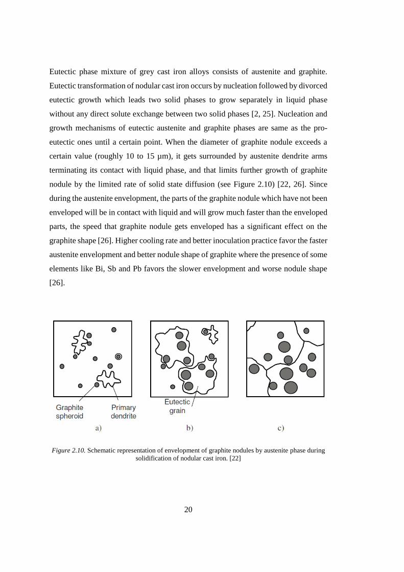
Eutectic phase mixture of grey cast iron alloys consists of austenite and graphite.

Eutectic transformation of nodular cast iron occurs by nucleation followed by divorced

eutectic growth which leads two solid phases to grow separately in liquid phase

without any direct solute exchange between two solid phases [2, 25]. Nucleation and

growth mechanisms of eutectic austenite and graphite phases are same as the pro-

eutectic ones until a certain point. When the diameter of graphite nodule exceeds a

certain value (roughly 10 to 15 µm), it gets surrounded by austenite dendrite arms

terminating its contact with liquid phase, and that limits further growth of graphite

nodule by the limited rate of solid state diffusion (see Figure 2.10) [22, 26]. Since

during the austenite envelopment, the parts of the graphite nodule which have not been

enveloped will be in contact with liquid and will grow much faster than the enveloped

parts, the speed that graphite nodule gets enveloped has a significant effect on the

graphite shape [26]. Higher cooling rate and better inoculation practice favor the faster

austenite envelopment and better nodule shape of graphite where the presence of some

elements like Bi, Sb and Pb favors the slower envelopment and worse nodule shape

[26].

Figure 2.10. Schematic representation of envelopment of graphite nodules by austenite phase during

solidification of nodular cast iron. [22]

21

2.5. Cooling Curve Thermal Analysis of Nodular Cast Iron

Although thermal analysis is a general term including all the analysis methods

measuring a change in a specific property of a substance as a result of a change in

temperature, in foundry industry cooling curve thermal analysis method is the most

practical one. Cooling curve thermal analysis is conducted by sampling certain amount

of liquid metal into a thermocouple inserted mould which lets us observe the cooling

curve of the sample during cooling, solidification and solid-state transformations by

means of temperature versus time graph. The obtained cooling curve is a result of heat

balance between the sample and its surroundings. When there is no phase

transformation, cooling curve represents the cooling of a liquid or solid substance, and

it has a constant negative slope indicating the cooling rate which depends on heat

transport conditions, mass and heat capacity of the substance. In the case of a phase

transformation, cooling curve is affected by the thermal consequences of the

transformation, and the change in slope depends on enthalpy of transformation and

the fraction of the transformed substance. If the transformation is a solidification, the

enthalpy change will be negative, so certain amount of heat will be evolved, and slope

of the cooling curve will move from its negative value in positive direction with a

magnitude determined by the latent heat of solidification and fraction of the

transformed substance.

Cooling curve of cast iron reveals various peculiarities letting us name the critical

points on cooling curve which may indicate some information on the sample

properties. It was observed in literature that nomenclature of these points varies

highly. The company OCC GmbH has one of the most informative description of

nomenclature of the points on the cooling curve and its first and second derivatives

with respect to time. Therefore, it can be a good example to understand the structure

of the cooling curve of cast iron. The critical points on the cooling curve were revealed

in Figure 2.11, and descriptions of the nomenclature were listed in Table 2.2 [27]. The

first derivative and second derivative curves are used to determine the critical points

so that zero points on the first derivative curve represent the arrests on the cooling

22

curve, and zero points on the second derivative curve represent the inflection points

on the cooling curve [27].

23

Figure 2.11. Illustration of the cooling curve of nodular cast iron melt with the first and second

derivatives indicating the main points. [27]

24

Table 2.2. Nomenclature and definition of the main points on a nodular cast iron cooling curve and

its first and second derivatives. [27]

Designation Unit Signification

Max °C Maximum temperature measured

LPM °C/s² Maximum at second derivative before liquidus

LPA °C/s² Highest temperature acceleration before liquidus

LiLo °C Minimum temperature measured before liquidus

Liq °C Liquidus temperature

LiUp °C Maximum temperature measured after liquidus

MIR °C Temperature with highest cooling rate before eutectic

EPA °C/s² Highest temperature acceleration before eutectic

EuLo °C Minimum temperature measured before eutectic

Eut °C Eutectic temperature

EuUp °C Maximum temperature measured after eutectic

EPM °C/s² Smallest temperature acceleration after eutectic

EBR °C Temperature at beginning of eutectic transformation

EER °C Temperature at end of eutectic transformation

EFA °C Temperature at fade of eutectic transformation

EoPre °C/s² Maximum temperature acceleration before EoF

EoF °C Temperature at end of solidification

EoPst °C/s² Minimum temperature acceleration after EoF

The early studies on cooling curve thermal analysis of cast iron revealed that

composition of cast iron has an effect on its cooling curve. For instance, it was

observed by Loper et al. that temperature of the first arrest on the cooling curve

decreases by increasing carbon equivalent until a certain point, and beyond this point

it starts increasing back, so that the first arrest represents the liquidus and the second

arrest represents the eutectic transformation [28]. Based on this knowledge, it was

proven by further studies that carbon equivalent value of hypo-eutectic alloys can be

calculated by using the liquidus temperature obtained from the cooling curve, and

carbon content can be calculated for those alloys by using liquidus and metastable

eutectic transformation temperatures obtained from the cooling curve of white

solidification [18].

25

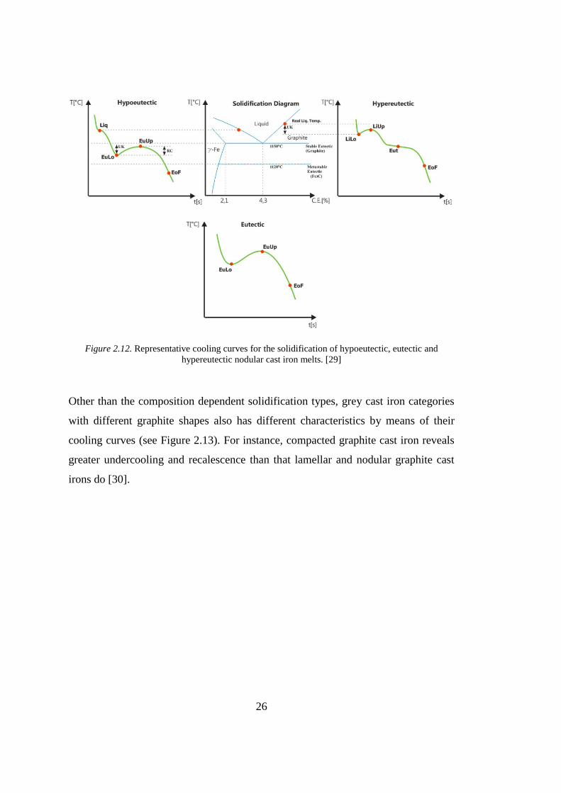
With the state-of-art technology, it is convenient to recognize the difference between

cooling curve characteristics of composition dependent solidification types. In Figure

2.12, the representative cooling curves and the correspondence with the phase diagram

for 3 different compositions are given [29]. The cooling curve on the left belongs to

hypoeutectic composition. The one on the right has hypereutectic composition, and

the one at the bottom is with eutectic or near-eutectic composition. On the cooling

curve of hypoeutectic nodular cast iron, the first arrest occurs at liquidus by the

nucleation and growth of austenite dendrites [27]. The second arrest represents the

eutectic transformation by the nucleation and growth of austenite-graphite eutectic

phase mixture [27]. Since nucleation of graphite requires excess energy, undercooling

is observed, and eutectic transformation occurs at a temperature lower than the

equilibrium transformation temperature which is seen on phase diagram [27]. Once

graphite growth starts, an increase in temperature is observed due to the released

energy as a result of carbon dissociation [27]. This phenomenon is named as

recalescence. Hypereutectic nodular cast iron also has a liquidus arrest, but unlike

hypoeutectic, it reveals undercooling and recalescence at liquidus because here

graphite nucleation and growth starts at liquidus instead of eutectic [27]. At eutectic

transformation, it doesn’t reveal undercooling and recalescence because almost all

graphite nucleation occurs between liquidus and eutectic [27]. Cooling curve of

eutectic or near-eutectic nodular cast iron does not reveal a liquidus arrest because the

solidification occurs only by the eutectic transformation [27].

26

Figure 2.12. Representative cooling curves for the solidification of hypoeutectic, eutectic and

hypereutectic nodular cast iron melts. [29]

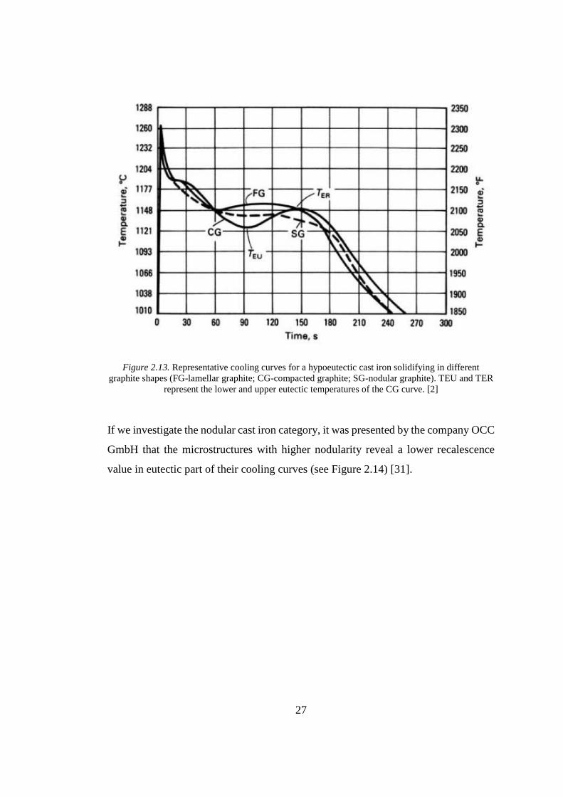
Other than the composition dependent solidification types, grey cast iron categories

with different graphite shapes also has different characteristics by means of their

cooling curves (see Figure 2.13). For instance, compacted graphite cast iron reveals

greater undercooling and recalescence than that lamellar and nodular graphite cast

irons do [30].

27

Figure 2.13. Representative cooling curves for a hypoeutectic cast iron solidifying in different

graphite shapes (FG-lamellar graphite; CG-compacted graphite; SG-nodular graphite). TEU and TER

represent the lower and upper eutectic temperatures of the CG curve. [2]

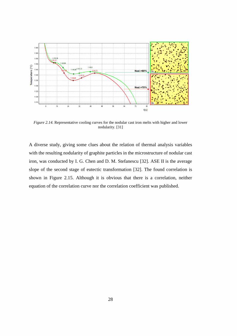
If we investigate the nodular cast iron category, it was presented by the company OCC

GmbH that the microstructures with higher nodularity reveal a lower recalescence

value in eutectic part of their cooling curves (see Figure 2.14) [31].

28

Figure 2.14. Representative cooling curves for the nodular cast iron melts with higher and lower

nodularity. [31]

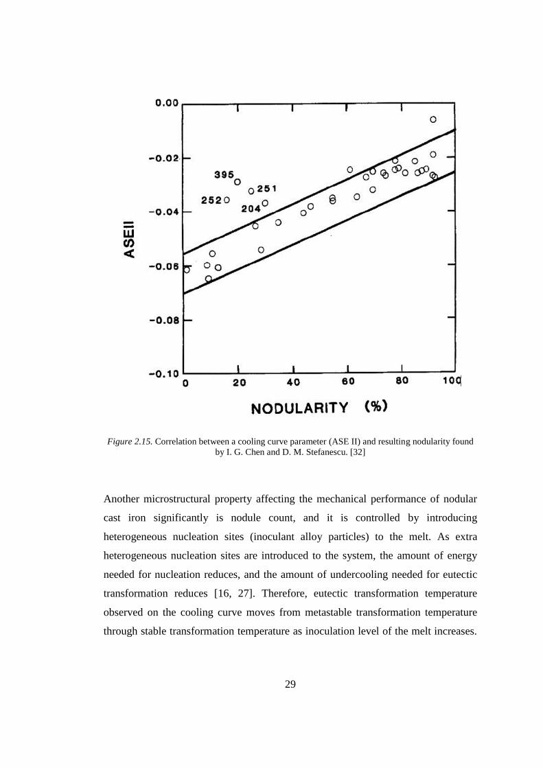
A diverse study, giving some clues about the relation of thermal analysis variables

with the resulting nodularity of graphite particles in the microstructure of nodular cast

iron, was conducted by I. G. Chen and D. M. Stefanescu [32]. ASE II is the average

slope of the second stage of eutectic transformation [32]. The found correlation is

shown in Figure 2.15. Although it is obvious that there is a correlation, neither

equation of the correlation curve nor the correlation coefficient was published.

29

Figure 2.15. Correlation between a cooling curve parameter (ASE II) and resulting nodularity found

by I. G. Chen and D. M. Stefanescu. [32]

Another microstructural property affecting the mechanical performance of nodular

cast iron significantly is nodule count, and it is controlled by introducing

heterogeneous nucleation sites (inoculant alloy particles) to the melt. As extra

heterogeneous nucleation sites are introduced to the system, the amount of energy

needed for nucleation reduces, and the amount of undercooling needed for eutectic

transformation reduces [16, 27]. Therefore, eutectic transformation temperature

observed on the cooling curve moves from metastable transformation temperature

through stable transformation temperature as inoculation level of the melt increases.

30

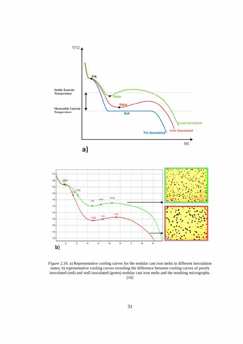
In Figure 2.16, the effect of inoculation level of the melt on its cooling curve and the

resulting microstructure was represented, and it is possible to mention that as

inoculation level of the melt increases, the amount of undercooling seen on the cooling

curve decreases, and the resulting graphite nodule count observed in the

microstructure increases.

31

Figure 2.16. a) Representative cooling curves for the nodular cast iron melts in different inoculation

states; b) representative cooling curves revealing the difference between cooling curves of poorly

inoculated (red) and well inoculated (green) nodular cast iron melts and the resulting micrographs.

[16]

32

A cooling curve thermal analysis cup is simply a thermocouple inserted mould

(typically made of sand by using a binder) which lets us observe temperature versus

time graph of the sample during cooling and solidification. The shape of the cooling

curve is determined by the balance between the latent heat liberated during

solidification and the heat lost to the surroundings [33]. Therefore, the design of the

test cup has a significant effect on the results and their interpretation [33]. As shown

in Figure 2.17, as the thickness of the cup sample decreases, undercooling increases

due to the increasing cooling rate as a result of decreasing modulus [33]. Therefore,

the effect of inoculation is more noticeable on the smaller size cups [33].

Figure 2.17. Schematic representation of the effect of cup sample thickness and state of inoculation

on the shape of the cooling curve of eutectic nodular cast iron melt. [33]

33

2.6. Active Oxygen Amount in Nodular Cast Iron

Oxygen found in nodular cast iron melt can be divided into two main groups which

are the oxygen content found in elemental form (also called active oxygen) and the

oxygen content found in chemical compounds (also called chemically bonded oxygen)

[34, 35]. Chemically bonded oxygen amount corresponds to the number of oxide

particles acting as heterogeneous nucleation sites for the graphite particles where

active oxygen amount relates the surface tension of iron and its interfacial energy with

graphite [36]. Therefore, in the nodular cast iron melt, too less oxygen content leads

to lack of heterogeneous nucleation sites for the graphite particles, and results in an

undesired microstructure where too high oxygen content leads to low interfacial

energy between iron and graphite which also results in an undesired microstructure

[36]. For this reason, oxygen content of the nodular cast iron melt needs to be

optimized for the desired microstructural properties.

Total amount of oxygen in a nodular cast iron specimen can be analyzed by

combustion analysis (LECO) tools. It is possible to measure the active oxygen amount

in nodular cast iron melt by special sensors with an electrochemical cell and a Pt-PtRh

(S-type) thermocouple [37]. The cell contains Cr-Cr2O3 as solid reference cell in

contact with MgO-stabilized ZrO2 solid-state electrolyte [37]. When the sensor is

immersed into the bath, an electrode made of iron contacts with the melt, and an

electro-voltaic cell is formed in between the reference cell and the melt [37]. A device

collecting the potential difference produced by the cell calculates the oxygen activity

[37].

The formula given in Equation 2.3 was established by the manufacturer (Heraeus

Electro-Nite Intl. NV) by modifying the Nernst equation with the known partial

pressure of oxygen in the reference cell [38].

Equation 2.3. log aO = 8.62 – {13580 – 10.08 (E + 24)} / T

34

Where aO is the oxygen activity of the melt, and it is considered as equal to the active

oxygen amount (in ppm), E is the electrical potential (in mV) produced by the cell,

and T is temperature (in °C) of the melt measured by Pt-PtRh thermocouple embedded

to the sensor [38].

A comprehensive study, aimed to find a relation between oxygen activity of the treated

nodular cast iron melt and the resulting microstructural properties, was conducted by

F. Mampaey et al. [37]. The results for three different melts are revealed in Figure

2.18. Although it is obvious that there is a correlation, neither equation of the

correlation curve nor the correlation coefficient was published.

35

Figure 2.18. The relation between active oxygen content of the nodular cast iron melt and the

resulting nodularity found by F. Mampaey et al. via the investigation of 3 different nodular cast iron

melts. [37]

37

CHAPTER 3

3. EQUIPMENTS, SAMPLES AND METHODOLOGY

3.1.Nodular Cast Iron Production Process

Mechanical performance of the fully ferritic nodular cast iron grades is highly

dependent on the nodularity and the nodule count which are much more difficult

to control than that the pearlite content is. Therefore, two fully ferritic nodular cast

iron grades which are EN-GJS-400-15 and EN-GJS-600-10C were investigated.

EN-GJS-600-10C is one of the new generation solution strengthened ferritic

ductile iron (SSFDI) grades which has mechanical properties competitive with

medium-carbon-steel grades, and a dedicated process control method is needed to

ensure its resulting performance.

Because they are highly preferred in the industry, the investigations were made on

hypoeutectic compositions.

To obtain results which are applicable to the industry, experimental data were

collected from the usual production of the foundry Ferromatrix NV.

Approximately 4 tons of base iron for nodular cast iron was prepared by using a

medium frequency induction furnace by charging pig iron for nodular cast iron

which has a sulphur content less than 0.02wt%, steel scrap to decrease the carbon

content, nodular cast iron returns to recycle and ferroalloys to achieve the aimed

chemical composition of the grades. To achieve the desired graphite shape while

keeping the inoculation potential above the critical state, sulphur content of the

base iron was kept at a degree of 0.01wt%. To keep the solidification shrinkage at

a low level without introducing tendency for undesired graphite forms, carbon

equivalent of the base iron was kept at a degree of 4.2wt% which is near to the

upper limit of hypoeutectic composition. The melting process was repeated 23

38

times (11 times for the alloy EN-GJS-400-18 and 12 times for the alloy EN-GJS-

600-10C).

After the charge was melted and reached to a temperature around 1500°C,

approximately 2000 kg of base iron is tapped to a preheated ladle, and a forklift

brought it to the ladle station for the Mg treatment. At the ladle station, open top

of the ladle was closed with a refractory lined steel cover which prevents splashing

and lowers the loss in heat, also the alloying elements in gas form. On the ladle

cover, there were three channels. One inlet for the cored wire with Mg master

alloy, one inlet for the cored wire with inoculant master alloy and one outlet for

the gas products of the reactions. The ladle is weighed by scale integrated to the

forklift and the net liquid base iron is calculated by subtracting the tare. The cored

wires with Mg and inoculant master alloys were fed by two electric motors

simultaneously. The length of the cored wires was calculated such that 0.42wt%

percent of Mg master alloy and 0.30wt% of inoculant master alloy were

introduced. After the treatment was completed, the ladle was moved to the

deslagging station. Fluidity of the slag which floats on the surface of liquid iron

was increased with the help of a flux (limestone), then deslagging was performed

to prevent dross inclusions. The ladle process was repeated 40 times (20 ladles for

the alloy EN-GJS-400-18 and 20 ladles for the alloy EN-GJS-600-10C) so that 20

heats for each grade were investigated. Chemical compositions of the cored wires

with Mg and inoculant mater alloys were revealed in Table 3.1 and Table 3.2

respectively.

39

Table 3.1. Chemical composition of the cored wire with Mg master alloy.

Cored Wire (g/m): 410

Unit Powder (Core) (g/m): 252

Content of the Core:

Si (%) Mg (%) Ca (%) Others (%)

50.4 25.8 4.2 19.6

Content per unit length:

Si (g/m) Mg (g/m) Ca (g/m) Others (g/m)

127.0 65.0 10.7 49.3

Table 3.2. Chemical composition of the cored wire with inoculation master alloy.

Cored Wire (g/m): 436

Unit Powder (Core) (g/m): 266

Content of the Core:

Si (%) Ca (%) Bi (%) Al (%) Rare Earth (%) Others (%)

67.2 1.4 0.9 0.8 0.7 29.0

Content per unit length

Si (g/m) Ca (g/m) Bi (g/m) Al (g/m) Rare Earth (g/m) Others (g/m)

178.8 3.7 2.4 2.1 1.9 77.1

40

Figure 3.1. Schematic representation of the process cycle applied for each ladle.

3.2. Active Oxygen Amount Measurement in Nodular Cast Iron Melt

For the active oxygen amount measurement in liquid cast iron, Celox FoundryTM

disposable sensors provided by Heraeus Electro-Nite Intl. NV were used. The

sensor contains an electro-voltaic cell and an S-type (Pt-PtRh10) thermocouple

[37]. The electro-voltaic cell contains an anode electrode made of molybdenum

connected to a closed end tube filled with Cr-Cr2O3 mixture as oxygen reference

material in contact with magnesia stabilized zirconia (MSZ) as a solid-state

electrolyte [37]. When the sensor is immersed in the bath, the cathode electrode

which is made of iron contacts with the melt, and an electro-voltaic cell is formed

between the oxygen reference cell and the melt [37].

A dedicated vibration lance for the accurate measurement of quite low oxygen

activities which are typical for Mg treated cast iron and a CF LabE-IVTM device

(provided by Heraeus Electro-Nite Intl. NV) collecting the potential differences

produced by the electrochemical cell and calculating the oxygen activity by a

formula based on Nernst equation was used [37]. The system was always

calibrated before the use.

41

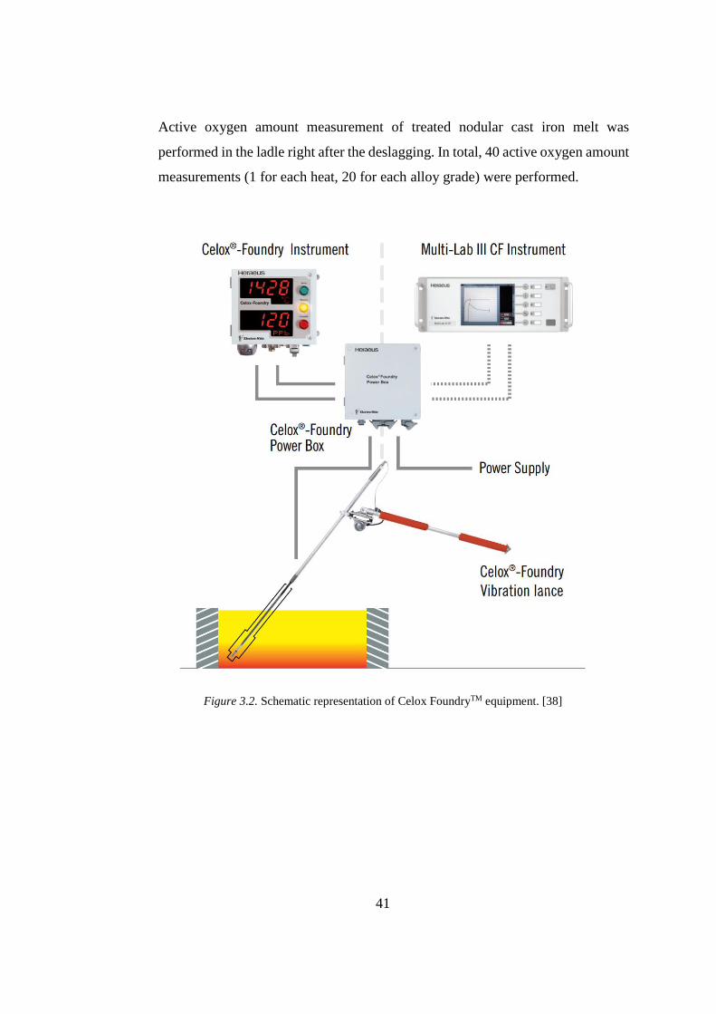
Active oxygen amount measurement of treated nodular cast iron melt was

performed in the ladle right after the deslagging. In total, 40 active oxygen amount

measurements (1 for each heat, 20 for each alloy grade) were performed.

Figure 3.2. Schematic representation of Celox FoundryTM equipment. [38]

42

3.3. Cooling Curve Thermal Analysis of Nodular Cast Iron Melt

For the cooling curve thermal analysis of nodular cast iron melt, recently

developed thermal analysis cups QuiKCup CoverTM provided by Heraeus Electro-

Nite Intl. NV were used (see Figure 3.3). QuiKCup CoverTM is a closed cup with

a cover on top which ensures the consistency of sample volume and cooling

conditions and decreases eventual variations in the results [39]. The ingate

between cover and cup chamber is closed by tapes from both inner and outer side,

so that it is possible to insert additives such as inoculant between those two tapes,

and those additives are dissolved homogeneously by the liquid alloy flowing

through the ingate (see Figure 3.4) [39]. QuiKCup CoverTM has a 12 mm of sample

thickness which is less than half of that the conventional cups do, and decreased

sample thickness ensures a more obvious and comparable eutectic undercooling

which is normally quite low for the solidification of inoculated nodular cast iron

melt [39]. QuiKCup CoverTM contains a K-type (Chromel-Alumel) thermocouple

with an accuracy of +/- 0.2°C which is five times more accurate than the

conventional cups, and higher thermocouple accuracy promises more accurate

experimental data [39].

43

Figure 3.3. Drawing of the QuiKCup CoverTM cut by the vertical middle plan (units: mm). 1- Shell

sand body; 2- Shell sand cover; 3- Tapes holding the inoculant at the ingate. [39]

Figure 3.4. Illustration for the mixing of the additives inserted to the ingate of QuiKCup CoverTM.

a) Right before the molten metal contacts to the cover; b) During the filling; c) Filled sample with

homogeneously mixed additive. [39]

44

QuiKLabE-IVTM devices (provided by Heraeus Electro-Nite Intl. NV) collecting the

potential differences produced by the thermocouple in the cup, converting them to the

corresponding temperature values and sending to the computer via Ethernet

connection were used [39]. The system was always calibrated before the use.

On the computer, a software MeltControl2020TM (provided by Heraeus Electro-Nite

Intl. NV) processing the incoming raw data, constructing temperature versus time

graph and its first derivative by applying a curve smoothing algorithm and identifying

the peculiarities on the curve was used [39]. The description and nomenclature of the

cooling curve parameters identified by the software were listed in Table 3.3. The

software saves all curves in a database and allows the export of the saved data to MS

Office Excel for further data evaluation.

45

Table 3.3. Description and nomenclature of the cooling curve parameters identified by

MeltControl2020TM. [39]

Abbreviation Unit Signification

TP (°C) Maximum temperature measured by the thermocouple

TP_dT (°C/s) Cooling rate at TP point

TP_t (s) Time at TP point

TL (°C) Liquidus temperature corresponding to the local

minimum at the derivative curve

TL_dT (°C/s) Cooling rate at TL point

TL_t (s) Time at TL point

TI (°C) Temperature between the liquidus and eutectic point

with the highest cooling rate

TI_dT (°C/s) Cooling rate at TI point

TI_t (s) Time at TI point

TEmin (°C) Minimum temperature measured before the eutectic

point

TEmin_t (s) Time at TEmin point

TEmax (°C) Maximum temperature measured after the eutectic

point

TEmax_t (s) Time at TEmax point

TE (°C) Eutectic temperature corresponding to the local

minimum in the derivative curve

TE_dT (°C/s) Cooling rate at TE point

TE_t (s) Time at TE point

TS (°C) Eutectic temperature (in the case of white

solidification)

TF (°C) End of solidification temperature corresponding to the

maximum cooling rate

TF_dT (°C/s) Cooling rate at TF point

TF_t (s) Time at TF point

DT (°C) Eutectic undercooling (1150°C - TEmin)

DTM (°C) Eutectic recalescence (TEmax - TEmin)

DTM_t (s) Eutectic recalescence duration (TEmax_t - TEmin_t)

TE_A (°) The angle between ITEmin,TEmaxI line and X-axis

(arctan(DTM/DTM_t))

TE_Z (°C*s) Area of the eutectic recalescence triangle

(DTM * DTM_t / 2)

FL_t (s) Duration of solidification (TF_t - TL_t)

46

To obtain varied cooling curves and microstructural properties, thermal analysis cups

with different additive contents were used. Two sets of data were collected. For the

first dataset, there were four thermal analysis stations for each heat; 1) Plain cup, 2)

The cup containing 0.05wt% SpherixTM inoculant (provided by FerroAtlantica SL), 3)

The cup containing 0.05wt% Spherix-PlusTM inoculant (provided by FerroAtlantica

SL) and 4) The cup containing 0.05wt% SMW 605TM inoculant (provided by ASK

Chemicals GmbH). For the second dataset, there were five thermal analysis stations

for each heat; 1) Plain cup, 2) The cup containing 0.05wt% SpherixTM inoculant

(provided by FerroAtlantica SL), 3) The cup containing 0.10wt% SpherixTM inoculant,

4) The cup containing 0.15wt% SpherixTM inoculant and 5) The cup containing

0.4wt% Te and 0.3wt% S providing white (metastable) solidification to obtain eutectic

transformation temperature of white solidification which might be useful to eliminate

the effect of Si content on the curve parameters. To ensure the homogeneous mixing

of the inoculants at the cup ingate, the inoculants were sieved, and the ones in a size

range of 125 µ and 355 µ were used. Chemical compositions of the inoculants which

were used as additives at the cup ingate are revealed in Table 3.4. In total, 160 cooling

curves thermal analysis of grey (stable) solidification (4 for each heat, 80 for each

alloy grade) and 20 cooling curve thermal analysis of white solidification (1 for each

heat of the second dataset, 10 for each alloy grade) were conducted (see Table 3.5).

Table 3.4. Chemical composition of the inoculants which were used as additives at the cup ingate.

Inoculant Spherix Spherix-plus SMW605

Si (%) 67.2 67.5 65.1

Ca (%) 1.4 1.6 2.1

Bi (%) 0.9 - 1.0

Al (%) 0.8 0.8 0.8

Rare Earth (%) 0.7 0.7 1.0

Sb (%) - 0.9 -

Others (%) 29.0 28.5 30.0

47

Table 3.5. List of the cooling curve thermal analysis samples.

Alloy ID Charge # Ladle # Cup # Content ID Content (%)

EN-GJS-400-18 1 1 1 Spherix 0.05

EN-GJS-400-18 1 1 2 Spherix+ 0.05

EN-GJS-400-18 1 1 3 SMW605 0.05

EN-GJS-400-18 1 1 4 - -

EN-GJS-400-18 2 2 5 Spherix 0.05

EN-GJS-400-18 2 2 6 Spherix+ 0.05

EN-GJS-400-18 2 2 7 SMW605 0.05

EN-GJS-400-18 2 2 8 - -

EN-GJS-400-18 2 3 9 Spherix 0.05

EN-GJS-400-18 2 3 10 Spherix+ 0.05

EN-GJS-400-18 2 3 11 SMW605 0.05

EN-GJS-400-18 2 3 12 - -

EN-GJS-400-18 3 4 13 Spherix 0.05

EN-GJS-400-18 3 4 14 Spherix+ 0.05

EN-GJS-400-18 3 4 15 SMW605 0.05

EN-GJS-400-18 3 4 16 - -

EN-GJS-400-18 4 5 17 Spherix 0.05

EN-GJS-400-18 4 5 18 Spherix+ 0.05

EN-GJS-400-18 4 5 19 SMW605 0.05

EN-GJS-400-18 4 5 20 - -

EN-GJS-400-18 4 6 21 Spherix 0.05

EN-GJS-400-18 4 6 22 Spherix+ 0.05

EN-GJS-400-18 4 6 23 SMW605 0.05

EN-GJS-400-18 4 6 24 - -

EN-GJS-400-18 5 7 25 Spherix 0.05

EN-GJS-400-18 5 7 26 Spherix+ 0.05

EN-GJS-400-18 5 7 27 SMW605 0.05

EN-GJS-400-18 5 7 28 - -

EN-GJS-400-18 5 8 29 Spherix 0.05

EN-GJS-400-18 5 8 30 Spherix+ 0.05

EN-GJS-400-18 5 8 31 SMW605 0.05

EN-GJS-400-18 5 8 32 - -

EN-GJS-400-18 6 9 33 Spherix 0.05

EN-GJS-400-18 6 9 34 Spherix+ 0.05

EN-GJS-400-18 6 9 35 SMW605 0.05

EN-GJS-400-18 6 9 36 - -

48

EN-GJS-400-18 6 10 37 Spherix 0.05

EN-GJS-400-18 6 10 38 Spherix+ 0.05

EN-GJS-400-18 6 10 39 SMW605 0.05

EN-GJS-400-18 6 10 40 - -

EN-GJS-400-18 7 11 41 - -

EN-GJS-400-18 7 11 42 Spherix 0.05

EN-GJS-400-18 7 11 43 Spherix 0.10

EN-GJS-400-18 7 11 44 Spherix 0.15

EN-GJS-400-18 7 11 W1 Te + S 0.4 + 0.3

EN-GJS-400-18 7 12 45 - -

EN-GJS-400-18 7 12 46 Spherix 0.05

EN-GJS-400-18 7 12 47 Spherix 0.10

EN-GJS-400-18 7 12 48 Spherix 0.15

EN-GJS-400-18 7 12 W2 Te + S 0.4 + 0.3

EN-GJS-400-18 8 13 49 - -

EN-GJS-400-18 8 13 50 Spherix 0.05

EN-GJS-400-18 8 13 51 Spherix 0.10

EN-GJS-400-18 8 13 52 Spherix 0.15

EN-GJS-400-18 8 13 W3 Te + S 0.4 + 0.3

EN-GJS-400-18 8 14 53 - -

EN-GJS-400-18 8 14 54 Spherix 0.05

EN-GJS-400-18 8 14 55 Spherix 0.10

EN-GJS-400-18 8 14 56 Spherix 0.15

EN-GJS-400-18 8 14 W4 Te + S 0.4 + 0.3

EN-GJS-400-18 9 15 57 - -

EN-GJS-400-18 9 15 58 Spherix 0.05

EN-GJS-400-18 9 15 59 Spherix 0.10

EN-GJS-400-18 9 15 60 Spherix 0.15

EN-GJS-400-18 9 15 W5 Te + S 0.4 + 0.3

EN-GJS-400-18 9 16 61 - -

EN-GJS-400-18 9 16 62 Spherix 0.05

EN-GJS-400-18 9 16 63 Spherix 0.10

EN-GJS-400-18 9 16 64 Spherix 0.15

EN-GJS-400-18 9 16 W6 Te + S 0.4 + 0.3

EN-GJS-400-18 10 17 65 - -

EN-GJS-400-18 10 17 66 Spherix 0.05

EN-GJS-400-18 10 17 67 Spherix 0.10

EN-GJS-400-18 10 17 68 Spherix 0.15

EN-GJS-400-18 10 17 W7 Te + S 0.4 + 0.3

49

EN-GJS-400-18 10 18 69 - -

EN-GJS-400-18 10 18 70 Spherix 0.05

EN-GJS-400-18 10 18 71 Spherix 0.10

EN-GJS-400-18 10 18 72 Spherix 0.15

EN-GJS-400-18 10 18 W8 Te + S 0.4 + 0.3

EN-GJS-400-18 11 19 73 - -

EN-GJS-400-18 11 19 74 Spherix 0.05

EN-GJS-400-18 11 19 75 Spherix 0.10

EN-GJS-400-18 11 19 76 Spherix 0.15

EN-GJS-400-18 11 19 W9 Te + S 0.4 + 0.3

EN-GJS-400-18 11 20 77 - -

EN-GJS-400-18 11 20 78 Spherix 0.05

EN-GJS-400-18 11 20 79 Spherix 0.10

EN-GJS-400-18 11 20 80 Spherix 0.15

EN-GJS-400-18 11 20 W10 Te + S 0.4 + 0.3

EN-GJS-600-10C 12 21 81 Spherix 0.05

EN-GJS-600-10C 12 21 82 Spherix+ 0.05

EN-GJS-600-10C 12 21 83 SMW605 0.05

EN-GJS-600-10C 12 21 84 - -

EN-GJS-600-10C 13 22 85 Spherix 0.05

EN-GJS-600-10C 13 22 86 Spherix+ 0.05

EN-GJS-600-10C 13 22 87 SMW605 0.05

EN-GJS-600-10C 13 22 88 - -

EN-GJS-600-10C 13 23 89 Spherix 0.05

EN-GJS-600-10C 13 23 90 Spherix+ 0.05

EN-GJS-600-10C 13 23 91 SMW605 0.05

EN-GJS-600-10C 13 23 92 - -

EN-GJS-600-10C 14 24 93 Spherix 0.05

EN-GJS-600-10C 14 24 94 Spherix+ 0.05

EN-GJS-600-10C 14 24 95 SMW605 0.05

EN-GJS-600-10C 14 24 96 - -

EN-GJS-600-10C 15 25 97 Spherix 0.05

EN-GJS-600-10C 15 25 98 Spherix+ 0.05

EN-GJS-600-10C 15 25 99 SMW605 0.05

EN-GJS-600-10C 15 25 100 - -

EN-GJS-600-10C 15 26 101 Spherix 0.05

EN-GJS-600-10C 15 26 102 Spherix+ 0.05

EN-GJS-600-10C 15 26 103 SMW605 0.05

EN-GJS-600-10C 15 26 104 - -

50

EN-GJS-600-10C 16 27 105 Spherix 0.05

EN-GJS-600-10C 16 27 106 Spherix+ 0.05

EN-GJS-600-10C 16 27 107 SMW605 0.05

EN-GJS-600-10C 16 27 108 - -

EN-GJS-600-10C 17 28 109 Spherix 0.05

EN-GJS-600-10C 17 28 110 Spherix+ 0.05

EN-GJS-600-10C 17 28 111 SMW605 0.05

EN-GJS-600-10C 17 28 112 - -

EN-GJS-600-10C 17 29 113 Spherix 0.05

EN-GJS-600-10C 17 29 114 Spherix+ 0.05

EN-GJS-600-10C 17 29 115 SMW605 0.05

EN-GJS-600-10C 17 29 116 - -

EN-GJS-600-10C 18 30 117 Spherix 0.05

EN-GJS-600-10C 18 30 118 Spherix+ 0.05

EN-GJS-600-10C 18 30 119 SMW605 0.05

EN-GJS-600-10C 18 30 120 - -

EN-GJS-600-10C 19 31 121 - -

EN-GJS-600-10C 19 31 122 Spherix 0.05

EN-GJS-600-10C 19 31 123 Spherix 0.10

EN-GJS-600-10C 19 31 124 Spherix 0.15

EN-GJS-600-10C 19 31 W11 Te + S 0.4 + 0.3

EN-GJS-600-10C 19 32 125 - -

EN-GJS-600-10C 19 32 126 Spherix 0.05

EN-GJS-600-10C 19 32 127 Spherix 0.10

EN-GJS-600-10C 19 32 128 Spherix 0.15

EN-GJS-600-10C 19 32 W12 Te + S 0.4 + 0.3

EN-GJS-600-10C 20 33 129 - -

EN-GJS-600-10C 20 33 130 Spherix 0.05

EN-GJS-600-10C 20 33 131 Spherix 0.10

EN-GJS-600-10C 20 33 132 Spherix 0.15

EN-GJS-600-10C 20 33 W13 Te + S 0.4 + 0.3

EN-GJS-600-10C 20 34 133 - -

EN-GJS-600-10C 20 34 134 Spherix 0.05

EN-GJS-600-10C 20 34 135 Spherix 0.10

EN-GJS-600-10C 20 34 136 Spherix 0.15

EN-GJS-600-10C 20 34 W14 Te + S 0.4 + 0.3

EN-GJS-600-10C 21 35 137 - -

EN-GJS-600-10C 21 35 138 Spherix 0.05

EN-GJS-600-10C 21 35 139 Spherix 0.10

51

EN-GJS-600-10C 21 35 140 Spherix 0.15

EN-GJS-600-10C 21 35 W15 Te + S 0.4 + 0.3

EN-GJS-600-10C 21 36 141 - -

EN-GJS-600-10C 21 36 142 Spherix 0.05

EN-GJS-600-10C 21 36 143 Spherix 0.10

EN-GJS-600-10C 21 36 144 Spherix 0.15

EN-GJS-600-10C 21 36 W16 Te + S 0.4 + 0.3

EN-GJS-600-10C 22 37 145 - -

EN-GJS-600-10C 22 37 146 Spherix 0.05

EN-GJS-600-10C 22 37 147 Spherix 0.10

EN-GJS-600-10C 22 37 148 Spherix 0.15

EN-GJS-600-10C 22 37 W17 Te + S 0.4 + 0.3

EN-GJS-600-10C 22 38 149 - -

EN-GJS-600-10C 22 38 150 Spherix 0.05

EN-GJS-600-10C 22 38 151 Spherix 0.10

EN-GJS-600-10C 22 38 152 Spherix 0.15

EN-GJS-600-10C 22 38 W18 Te + S 0.4 + 0.3

EN-GJS-600-10C 23 39 153 - -

EN-GJS-600-10C 23 39 154 Spherix 0.05

EN-GJS-600-10C 23 39 155 Spherix 0.10

EN-GJS-600-10C 23 39 156 Spherix 0.15

EN-GJS-600-10C 23 39 W19 Te + S 0.4 + 0.3

EN-GJS-600-10C 23 40 157 - -

EN-GJS-600-10C 23 40 158 Spherix 0.05

EN-GJS-600-10C 23 40 159 Spherix 0.10

EN-GJS-600-10C 23 40 160 Spherix 0.15

EN-GJS-600-10C 23 40 W20 Te + S 0.4 + 0.3

3.4. Metallographic Evaluation

After the sampling was made, samples from the thermal analysis cups were labeled

indicating the heat number and the cup content. All the cups with grey

solidification (160 cups) were subjected to metallographic sampling, specimen

preparation and image analysis. After cleaning the sand from the sample’s surface,

it was cut from its horizontal plane from approximately 2 mm below the quartz

tube of the thermocouple by using an abrasive cutter with boron-based cooling

liquid. The lower part of each cut samples was used for the metallographic

52

investigation on the cut surface as presented in Figure 3.5. Since it has the

microstructure most corresponding to the obtained cooling curve, the closest part

possible without having quartz inclusions was chosen. After molding the samples

into Epoxy, standard metallographic specimen preparation steps were followed.

Grinding for 1 minute by 120 mesh grinding paper, for 1 minute by 200 mesh

grinding paper, for 1 minute by 600 mesh grinding paper and for 2 minutes by 800

mesh grinding paper were applied respectively by washing the samples after each

step. Polishing for 9 minutes by using 3 µm diamond suspension was applied, then

the surface was cleaned with Ethanol and dried with hot air. The grinding and

polishing operations were done by using AbraminTM machine, grinding papers and

DiaProPlusTM polishing suspension all provided by Struers GmbH.

Metallographic evaluation was done right after polishing and cleaning to observe

the graphite phase clearly. Then, the specimens were etched for approximately 4

seconds by using 2vol% Nital Ethanol solution for the investigation of the matrix.

The specimens were investigated under a 3-megapixel digital camera mounted to

Nikon OptiPhotTM metallographic microscope using 5x, 10x, 20x or 50x

magnifications. The metallographic evaluation of the specimens was conducted by

using the image analysis software Micr-O-PhaseTM provided by Heraeus Electr-

Nite Intl. NV. The software gets the micrographs directly from the camera

mounted to microscope which was calibrated by using a scale with 10 µm of sub-

divisions, and the information of used magnification is shared by the software [40].

The pixel size in a micrograph is a function of camera’s resolution and the used

magnification [40]. Since the software has the necessary information, it is able to

calculate distances and areas by counting the pixels and using the pixel size [40].

Then, by using several algorithms, the software analyses all the metallographic

parameters such as nodularity, nodule count, phase area of graphite, graphite shape

classification, ferrite and pearlite ratios all according to the norm EN-ISO-945-1

[40].

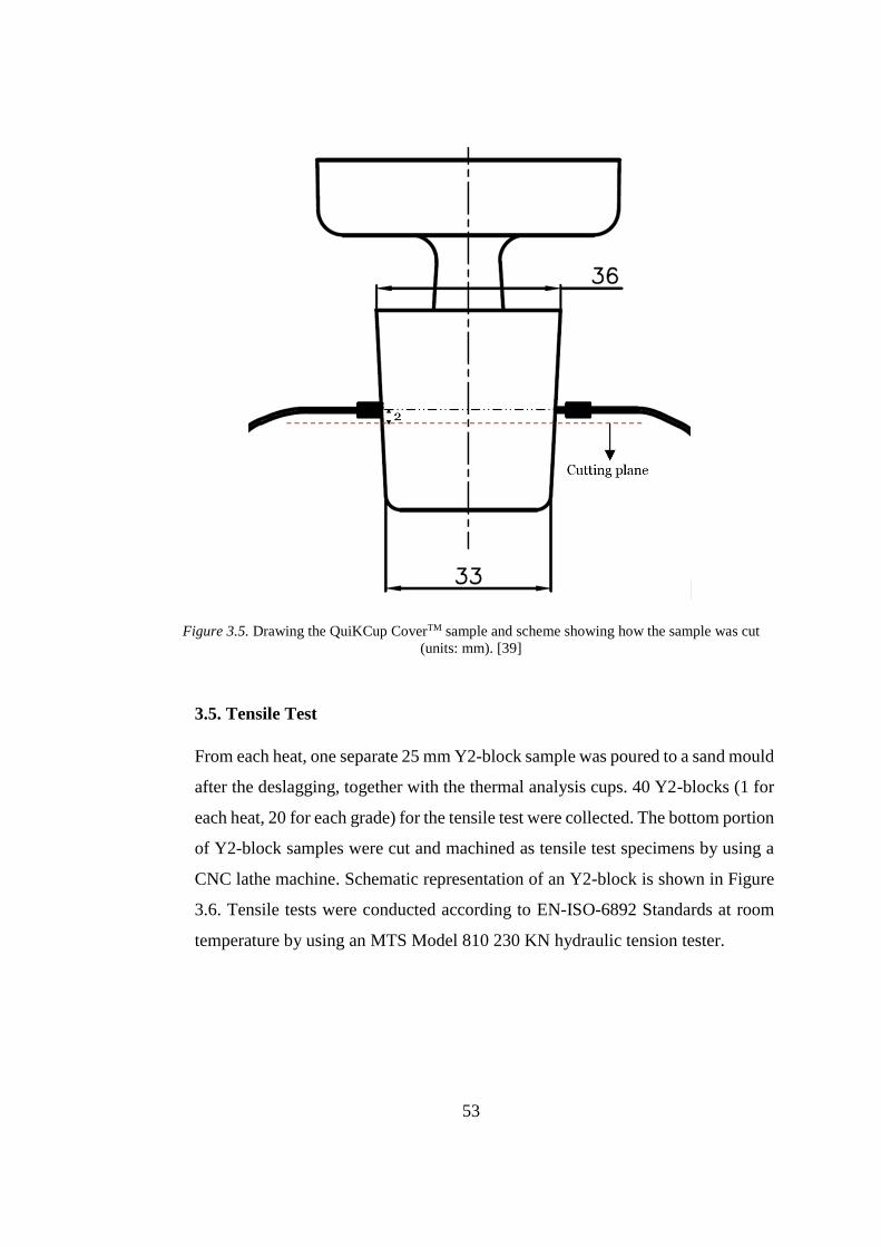
53

Figure 3.5. Drawing the QuiKCup CoverTM sample and scheme showing how the sample was cut

(units: mm). [39]

3.5. Tensile Test

From each heat, one separate 25 mm Y2-block sample was poured to a sand mould

after the deslagging, together with the thermal analysis cups. 40 Y2-blocks (1 for

each heat, 20 for each grade) for the tensile test were collected. The bottom portion

of Y2-block samples were cut and machined as tensile test specimens by using a

CNC lathe machine. Schematic representation of an Y2-block is shown in Figure

3.6. Tensile tests were conducted according to EN-ISO-6892 Standards at room

temperature by using an MTS Model 810 230 KN hydraulic tension tester.

54

Figure 3.6. Schematic representation of a tensile test specimen (units: mm). [41]

3.6. Optical Emission Spectroscopy

From each heat, a coin sample was poured to a steel mold with copper die, ensuring

unidirectional white (metastable) solidification, after the deslagging, together with

the thermal analysis cups. 40 coin samples (1 for each heat, 20 for each alloy

grade) for chemical analysis by using optical emission spectroscopy (OES) were

collected. The coin samples were grinded and analyzed according to EN-ISO-

1083 Standards by using an OBLF QSN 750-II OES.

3.7. Data Correlation

The data acquired from the mentioned methods of analysis (cooling curve thermal

analysis, oxygen activity analysis, metallographic image analysis, optical emission

spectroscopy analysis and tensile test) revealing the process variables and resulting

55

properties were stored in MS Office Excel sheets, and then imported to the linear

regression software CSLTM developed by OCC GmbH. The linear regression

software evaluates the existing correlations between process variables and

resulting properties by analyzing the influence of one or more variables on a

chosen parameter and lists the evaluated linear regressions by plotting calculated

values versus measured values of the chosen parameter [42]. The software also

calculates r-square, T-test and F-test values of each regression [42].

57

CHAPTER 4

4. RESULTS AND DISCUSSION

4.1. Chemical Analysis

Chemical analysis results from optical emission spectroscopy (OES) and active

oxygen measurement results from Celox FoundryTM were revealed in Table 4.1.

Table 4.1. Chemical analysis results obtained by OES and Celox FoundryTM conducted after the Mg

treatment.

Alloy Charge Ladle C Si S Mn Cu Sn Mg aO

EN-GJS # # % % % % % % % ppb

400-18 1 1 3.44 2.58 0.007 0.16 0.014 0.003 0.043 63

400-18 2 2 3.45 2.54 0.007 0.20 0.037 0.003 0.046 64

400-18 2 3 3.36 2.54 0.006 0.18 0.031 0.003 0.049 64

400-18 3 4 3.49 2.60 0.006 0.21 0.025 0.003 0.052 66

400-18 4 5 3.45 2.53 0.006 0.14 0.019 0.003 0.044 64

400-18 4 6 3.41 2.46 0.005 0.13 0.014 0.003 0.051 62

400-18 5 7 3.44 2.57 0.005 0.16 0.021 0.003 0.049 63

400-18 5 8 3.43 2.50 0.005 0.19 0.021 0.003 0.050 65

400-18 6 9 3.45 2.48 0.006 0.18 0.038 0.003 0.046 60

400-18 6 10 3.47 2.53 0.006 0.16 0.034 0.003 0.052 63

400-18 7 11 3.48 2.46 0.006 0.19 0.015 0.003 0.050 61

400-18 7 12 3.47 2.52 0.007 0.16 0.013 0.003 0.040 62

400-18 8 13 3.47 2.44 0.006 0.21 0.056 0.003 0.046 62

400-18 8 14 3.48 2.48 0.007 0.21 0.057 0.003 0.044 61

400-18 9 15 3.47 2.46 0.006 0.17 0.007 0.003 0.048 62

400-18 9 16 3.48 2.51 0.007 0.16 0.007 0.003 0.043 76

400-18 10 17 3.47 2.36 0.007 0.17 0.009 0.002 0.045 59

400-18 10 18 3.37 2.47 0.006 0.17 0.009 0.003 0.046 61

400-18 11 19 3.46 2.43 0.007 0.15 0.035 0.004 0.049 62

400-18 11 20 3.47 2.39 0.007 0.14 0.028 0.004 0.048 59

58

600-10C 12 21 2.90 4.20 0.007 0.16 0.010 0.005 0.050 65

600-10C 13 22 2.84 4.09 0.005 0.17 0.016 0.005 0.049 68

600-10C 13 23 2.83 4.20 0.006 0.17 0.015 0.005 0.047 61

600-10C 14 24 2.84 4.15 0.006 0.19 0.013 0.005 0.049 66

600-10C 15 25 2.85 4.08 0.005 0.15 0.018 0.005 0.054 61

600-10C 15 26 2.83 4.11 0.005 0.16 0.019 0.005 0.051 62

600-10C 16 27 2.85 4.19 0.006 0.18 0.026 0.005 0.050 63

600-10C 17 28 2.82 4.17 0.005 0.17 0.013 0.005 0.051 63

600-10C 17 29 2.88 4.11 0.006 0.16 0.015 0.005 0.046 65

600-10C 18 30 2.92 4.10 0.006 0.23 0.018 0.005 0.055 63

600-10C 19 31 2.77 4.13 0.006 0.17 0.009 0.005 0.044 67

600-10C 19 32 2.80 4.18 0.006 0.17 0.009 0.005 0.045 64

600-10C 20 33 2.95 4.10 0.006 0.17 0.035 0.006 0.052 66

600-10C 20 34 2.88 4.11 0.005 0.17 0.034 0.006 0.049 60

600-10C 21 35 2.76 4.01 0.005 0.16 0.058 0.006 0.040 74

600-10C 21 36 2.91 4.06 0.006 0.17 0.057 0.006 0.048 66

600-10C 22 37 2.92 4.06 0.006 0.21 0.033 0.006 0.056 59

600-10C 22 38 2.91 4.12 0.007 0.21 0.033 0.006 0.052 62

600-10C 23 39 2.95 4.12 0.006 0.20 0.031 0.006 0.050 69

600-10C 23 40 2.92 4.10 0.006 0.20 0.031 0.006 0.049 65

Carbon is the main alloying element for the regular cast iron grades. It forms the

graphite phase which is characteristic for grey cast iron; and together with iron, it

forms cementite (Fe3C) which is characteristic for white cast iron, also a component

of pearlite eutectoid phase mixture which is common for most of the cast iron and

steel grades. For nodular cast iron grades, insufficient carbon content yields in a low

amount of graphite phase which may result in high solidification shrinkage and high

feeding needs because graphite formation provides a volume expansion during cast

iron solidification. It may also yield in a low ductility of the resulting material because

graphite phase in the structure provides elongation to ductile iron grades. Insufficient

carbon content increases the tendency to have a metastable eutectic transformation

forming carbides in the structure which result in a lower ductility and machinability.

On the other hand, excessive carbon content results in a hyper-eutectic composition

favoring some degenerated graphite forms and graphite floatation which have negative

59

effects on the resulting mechanical properties. Hyper-eutectic solidification provides

a higher amount of graphite formation and volume expansion, but most of the graphite

is formed before the eutectic transformation, and solid barrier formation on top of the

risers, so most of the volume expansion is useless in terms of feeding needs. For the

alloy EN-GJS-400-18, carbon is the main alloying element, and the target range for

carbon content of this alloy that was set by the foundry is from 3.35% to 3.50%. As

can be seen in Table 4.1, all the EN-GJS-400-18 specimens have carbon contents

within the target range. Since the alloy EN-GJS-600-10C has silicon as the main

alloying element, and it contributes to the carbon equivalent (C.E.), target range for

carbon content of this alloy that was set by the foundry is from 2.80% to 2.95% in

order to have a hypo-eutectic solidification. As can be seen in Table 4.1, the specimens

from ladle 31 and 35 have carbon contents below the lower limit of the target range.

In microstructural image analysis results (see Table 4.4), it can be seen that the

specimens from ladle 31 and 35 have the lowest graphite phase area percentage among

all the specimens which can be explained by the insufficient carbon content.

Silicon is a crucial alloying element for all grey cast iron grades. It increases the stable

eutectic transformation temperature and decreases the metastable one so that those

two transformation temperatures get farther from each other, and the possibility to

have a stable eutectic solidification increases. Therefore, it is known as a graphite

former. Since they both are necessary for graphite formation, silicon’s being

insufficient or excessive yields in similar tendencies as carbon’s does. For solution

strengthened ferritic ductile iron (SSFDI) grades, silicon content is even higher than

carbon content because there, silicon has another function in addition to being graphite

former. Silicon atoms act as solute atoms in ferrite structure resulting in lattice strains

which impedes the dislocation movement, thus provide solution strengthening. Unlike

ferritic-pearlitic matrix, solution strengthened ferritic matrix does not decrease the

ductility dramatically while increasing the strength. Also, with solution strengthened

ferritic matrix, strengthening is much more consistent among the sections with

different level of cooling rate than it is with ferritic-pearlitic matrix. Therefore, for

60

SSFDI grades, in the case of insufficient silicon content, less strain to be formed in

ferritic matrix structure may result in a lower strength. On the other hand, in the

literature, there are some studies claiming that both strength and ductility of SSFDI

grades make a peak at around 4.3%Si, then they drop dramatically due to the formation

of some brittle forms and the graphite degeneration [43, 44]. For the alloy EN-GJS-

400-18, the target range for silicon content that was set by the foundry is from 2.30%

to 2.60%. For EN-GJS-600-10C which is an SSFDI grade, it is from 4.00% to 4.30%.

As can be seen in Table 4.1, all the specimens from both alloys have silicon contents

within the target ranges.

Sulphur and oxygen are the surface-active elements reducing the interface energy

between iron and graphite. Therefore, decreasing their content in elemental form

makes increasing the volume/surface-area ratio of the graphite particles

thermodynamically more feasible, so it makes spherical graphite shape more stable.

Therefore, excess amount of sulphur and oxygen may decrease the nodularity and

affect the resulting mechanical properties negatively. On the other hand, according to

T. Skaland et al., heterogeneous nucleation sites for graphite nucleation are complex,

multi-layer sulphide-oxide inclusions [23]. Therefore, insufficient amount of sulphur

and oxygen may limit the number of heterogeneous nucleation sites to be formed, thus

the resulting graphite nodule count, and affect the mechanical properties negatively.

For both alloys, the target range for sulphur content that was set by the foundry is from

0.005% to 0.008%. As can be seen in Table 4.1, all the specimens from both alloys

have sulphur contents within the target range. For the active oxygen amount, the target

range is from 60 ppb to 70 ppb. As can be seen in Table 4.1, the specimens from ladles

17, 20 and 37 have active oxygen contents below the lower limit where the ones from

ladles 16 and 35 are above the upper limit. Since there are many parameters which

may affect the nodularity and the nodule count, it is difficult to see the effect of slightly

lower or higher active oxygen content on the resulting microstructure.

Magnesium is introduced to the base iron of the nodular cast iron melts by a process

named as magnesium treatment, and its objective is to nodularize the graphite particle

61

shape by decreasing the content of surface active elements (sulphur and oxygen) and

increasing the interface energy between iron and graphite, so its effect is basically

reverse of the effect of sulphur and oxygen. Insufficient magnesium content decreases

the stability of spherical shape of the graphite and decreases the nodularity which may

affect the resulting mechanical properties negatively. On the other hand, excessive

magnesium content lowers the contents of sulphur and oxygen excessively, and it may

limit the nodule count in the resulting structure, thus the mechanical properties. Since

magnesium is a carbide former, its excess content may also induce the carbide

formation which has a negative effect on the ductility and machinability. For both

alloys, the target range for magnesium content that was set by the foundry is from

0.040% to 0.055%. As can be seen in Table 4.1, only the specimen from ladle 37 has

a magnesium content above the upper limit, and the rest are in the range. Since it is

just above the limit, it is difficult see its effect on the resulting properties.

Manganese is an important alloying element for lamellar graphite cast iron because it

prevents the formation of FeS which segregates at the grain boundaries, and it forms

MnS which is distributed homogeneously. To produce nodular cast iron, the melt is

treated by magnesium which bonds the sulphur, so there is no need for manganese. In

addition, manganese favors the pearlite formation, also excessive content of

manganese may result in metastable eutectic transformation. Since both alloys are

fully ferritic, the maximum manganese content for both alloys that was set by the

foundry is 0.25%. As can be seen in Table 4.1, all the specimens from both alloys have

manganese contents below the limit.

Copper and tin are also pearlite stabilizers, so they decrease the resulting ductility

while increasing the strength. Tin is a stronger pearlite stabilizer than that copper is,

so that much less amount of tin enough to achieve the same pearlite content achieved

by much more copper content. Since both alloys are fully ferritic, the maximum copper

and tin contents for both alloys that were set by the foundry are 0.06% and 0.006%

respectively. As can be seen in Table 4.1, all the specimens from both alloys have

copper and tin contents within the target range.

62

Active oxygen amount versus alloy grade chart is revealed in Figure 4.1 as box chart.

In the lamellar grey iron or the base iron of the nodular cast iron, amount of active

oxygen is mainly determined by silicon because it has the highest oxygen affinity at a

typical temperature of cast iron melt preparation. And, both alloy types were treated

by the same ratio of Mg master alloy. Therefore, one could expect the high silicon

alloy grade to have a lower content of active oxygen, but by looking at Figure 4.1, it

can be said that this is not the case. The reason may be that an active oxygen content

of 60 to 70 ppb is already too low so that the effect of having less oxygen before the

treatment is not visible on these resulting values.

Figure 4.1. Active oxygen amount (aO) versus alloy grade.

EN-GJS-400-18 EN-GJS-600-10C55

60

65

70

75

80

aO

(ppb)

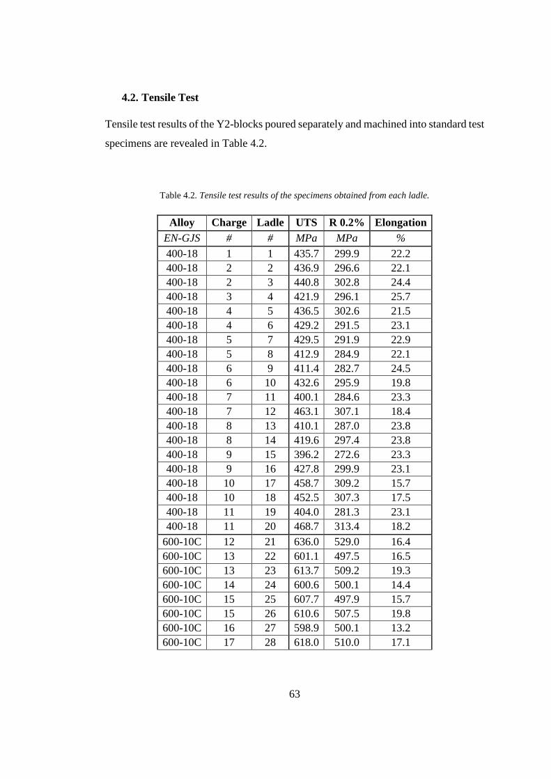
63

4.2. Tensile Test

Tensile test results of the Y2-blocks poured separately and machined into standard test

specimens are revealed in Table 4.2.

Table 4.2. Tensile test results of the specimens obtained from each ladle.

Alloy Charge Ladle UTS R 0.2% Elongation

EN-GJS # # MPa MPa %

400-18 1 1 435.7 299.9 22.2

400-18 2 2 436.9 296.6 22.1

400-18 2 3 440.8 302.8 24.4

400-18 3 4 421.9 296.1 25.7

400-18 4 5 436.5 302.6 21.5

400-18 4 6 429.2 291.5 23.1

400-18 5 7 429.5 291.9 22.9

400-18 5 8 412.9 284.9 22.1

400-18 6 9 411.4 282.7 24.5

400-18 6 10 432.6 295.9 19.8

400-18 7 11 400.1 284.6 23.3

400-18 7 12 463.1 307.1 18.4

400-18 8 13 410.1 287.0 23.8

400-18 8 14 419.6 297.4 23.8

400-18 9 15 396.2 272.6 23.3

400-18 9 16 427.8 299.9 23.1

400-18 10 17 458.7 309.2 15.7

400-18 10 18 452.5 307.3 17.5

400-18 11 19 404.0 281.3 23.1

400-18 11 20 468.7 313.4 18.2

600-10C 12 21 636.0 529.0 16.4

600-10C 13 22 601.1 497.5 16.5

600-10C 13 23 613.7 509.2 19.3

600-10C 14 24 600.6 500.1 14.4

600-10C 15 25 607.7 497.9 15.7

600-10C 15 26 610.6 507.5 19.8

600-10C 16 27 598.9 500.1 13.2

600-10C 17 28 618.0 510.0 17.1

64

600-10C 17 29 632.0 528.0 16.8

600-10C 18 30 605.0 501.0 18.0

600-10C 19 31 600.8 499.7 14.5

600-10C 19 32 610.0 515.0 13.2

600-10C 20 33 620.3 519.1 15.3

600-10C 20 34 621.1 519.7 15.1

600-10C 21 35 598.1 497.6 13.8

600-10C 21 36 610.0 507.9 17.3

600-10C 22 37 603.1 500.5 18.9

600-10C 22 38 600.9 501.8 18.6

600-10C 23 39 599.0 501.4 14.2

600-10C 23 40 600.2 501.9 14.1

Since design of the structures is done by considering the mechanical properties of the

materials to be used, tensile test results are significant in defining the material

performance, and they take place in the technical specifications of almost all

engineering materials. As indicated by their names in the standards, for the grade EN-

GJS-400-18, minimum ultimate tensile strength requirement is 400 MPa, and

minimum total elongation requirement is 18%, where for the grade EN-GJS-600-10C,

these values are 600 MPa and 10%. Alloy EN-GJS-400-18 is widely used in

applications where high material elongation is required even at low ambient

temperatures, and a mild strength is enough which is getting popular in wind energy

industry. On the other hand, alloy EN-GJS-600-10C provides a high strength without

a dramatic loss in ductility as a result of its solution strengthened ferritic matrix instead

of pearlitic-ferritic matrix, and it is getting popular in heavy-duty machine industry to

replace some of plain-carbon-steel grades. As can be seen in Table 4.2, the specimens

from the ladles 15, 27, 35 and 39 have ultimate tensile strength values slightly below

the minimum requirement, and the ones from the ladles 17 and 18 have total

elongation values below the minimum requirement. Since the process defines the

microstructure and the microstructure defines the performance, it could be expected

to find explanations for the out of specification specimens by means of microstructural

properties, thus the process parameters, but there could not be found, and this can be

65

explained by that the Y2-blocks samples for the tensile test were poured separately,

and they had different cooling conditions, where the metallographic specimens were

obtained from thermal analysis cup samples in order to observe the microstructures

corresponding the cooling curves.

4.3. Cooling Curve Thermal Analysis

The main results obtained from the cooling curves by using thermal analysis cups with

various contents are listed in Table 4.3.

Table 4.3. The main results of cooling curve thermal analysis indicating contents of the analysis cups

(Content types; 1-SpherixTM inoculant, 2-Sperix-PlusTM inoculant, 3-SMW605TM inoculant, 4-Te and

S).

Ladle Cup Content TL TEmin TE TE/dt TEmax TF TF/dt

# # Type % °C °C °C °C/s °C °C °C/s

1 1 1 0.05 1166.4 1148.4 1149.4 0.6 1152.3 1100.0 -5.4

1 2 2 0.05 1167.6 1146.3 1148.6 0.7 1152.0 1088.2 -4.8

1 3 3 0.05 1166.1 1147.8 1149.1 0.4 1151.2 1122.3 -4.7

1 4 - - 1166.2 1134.7 1138.4 0.9 1145.2 1085.8 -4.4

2 5 1 0.05 1166.5 1148.0 1149.1 0.5 1151.7 1098.0 -4.8

2 6 2 0.05 1167.4 1145.6 1148.0 0.8 1152.0 1089.4 -5.1

2 7 3 0.05 1166.8 1147.6 1148.4 0.4 1151.1 1093.7 -5.2

2 8 - - 1164.3 1133.8 1138.3 1.1 1144.6 1085.4 -5.0

3 9 1 0.05 1169.5 1147.1 1148.9 0.6 1151.9 1099.5 -4.5

3 10 2 0.05 1170.0 1145.8 1148.0 0.7 1152.5 1092.7 -4.7

3 11 3 0.05 1169.5 1147.0 1148.7 0.6 1152.3 1100.8 -5.0

3 12 - - 1168.3 1131.5 1136.5 1.1 1143.5 1086.2 -4.4

4 13 1 0.05 1158.4 1147.2 1148.5 0.6 1151.7 1112.8 -4.6

4 14 2 0.05 1158.8 1146.5 1148.3 0.7 1152.0 1087.4 -4.7

4 15 3 0.05 1158.7 1147.4 1148.7 0.5 1151.1 1119.5 -4.3

4 16 - - 1157.2 1122.2 1127.5 1.5 1136.3 1106.8 -3.2

5 17 1 0.05 1166.5 1148.6 1149.8 0.4 1152.0 1097.1 -4.9

5 18 2 0.05 1166.3 1146.7 1148.7 0.6 1151.4 1089.8 -5.4

5 19 3 0.05 1166.5 1149.2 1150.1 0.4 1152.1 1098.6 -4.9

66

5 20 - - 1166.3 1134.5 1138.3 1.0 1144.0 1081.6 -4.9

6 21 1 0.05 1171.3 1147.2 1148.2 0.5 1150.9 1092.0 -5.4

6 22 2 0.05 1173.8 1145.7 1148.3 0.7 1151.9 1089.3 -5.3

6 23 3 0.05 1172.2 1147.6 1149.3 0.6 1151.9 1095.7 -6.1

6 24 - - 1172.8 1130.1 1135.8 1.3 1141.9 1089.1 -6.0

7 25 1 0.05 1161.5 1146.2 1147.8 0.6 1150.4 1089.9 -5.5

7 26 2 0.05 1162.4 1143.3 1145.7 0.8 1149.5 1085.4 -5.5

7 27 3 0.05 1161.3 1147.2 1148.3 0.6 1150.9 1097.9 -5.8

7 28 - - 1161.2 1132.4 1137.3 1.2 1144.0 1088.7 -5.3

8 29 1 0.05 1164.8 1143.6 1145.8 0.8 1149.2 1090.1 -6.2

8 30 2 0.05 1163.9 1140.2 1143.8 0.9 1148.7 1086.9 -5.1

8 31 3 0.05 1163.0 1147.1 1148.2 0.5 1151.0 1095.7 -5.8

8 32 - - 1161.7 1124.1 1129.4 1.4 1137.7 1080.8 -5.3

9 33 1 0.05 1168.0 1146.7 1148.8 0.7 1152.2 1099.7 -4.8

9 34 2 0.05 1166.8 1142.3 1145.1 0.9 1149.6 1087.8 -4.9

9 35 3 0.05 1167.8 1145.8 1147.5 0.7 1151.6 1093.9 -5.6

9 36 - - 1167.9 1126.4 1132.4 1.4 1140.7 1087.2 -5.3

10 37 1 0.05 1162.0 1147.8 1149.9 0.6 1152.2 1089.8 -4.5

10 38 2 0.05 1164.7 1148.5 1150.1 0.7 1154.3 1097.3 -4.6

10 39 3 0.05 1162.5 1148.1 1149.8 0.4 1151.6 1119.7 -4.9

10 40 - - 1163.2 1129.4 1134.1 1.3 1143.1 1086.9 -4.3

11 41 - - 1159.1 1129.7 1133.8 1.1 1140.2 1076.9 -4.7

11 42 1 0.05 1161.5 1142.7 1144.3 0.6 1147.5 1088.1 -5.3

11 43 1 0.10 1161.0 1144.9 1145.8 0.4 1148.4 1089.9 -5.5

11 44 1 0.15 1161.2 1145.3 1146.7 0.6 1149.9 1088.7 -5.6

11 W1 4 0.70 1161.9 - 1108.4 - - - -

12 45 - - 1156.7 1132.9 1136.7 0.9 1142.6 1076.6 -4.2

12 46 1 0.05 1158.7 1148.1 1148.9 0.4 1151.4 1115.5 -4.9

12 47 1 0.10 1159.1 1148.8 1149.8 0.4 1151.9 1119.2 -5.0

12 48 1 0.15 1158.6 1147.9 1149.1 0.5 1151.4 1119.8 -5.0

12 W2 4 0.70 1158.9 - 1107.1 - - - -

13 49 - - 1161.9 1125.9 1129.4 1.0 1136.2 1097.1 -4.0

13 50 1 0.05 1163.5 1145.2 1147.3 0.7 1150.7 1103.1 -5.0

13 51 1 0.10 1162.6 1147.0 1148.5 0.5 1151.0 1095.4 -5.0

13 52 1 0.15 1161.6 1146.6 1147.7 0.5 1150.6 1092.0 -4.9

13 W3 4 0.70 1159.5 - 1108.4 - - - -

14 53 - - 1158.2 1125.1 1129.8 1.0 1136.0 1095.0 -3.9

14 54 1 0.05 1160.8 1146.2 1148.0 0.5 1150.9 1115.6 -4.5

14 55 1 0.10 1161.1 1149.5 1150.3 0.4 1152.0 1121.4 -4.6

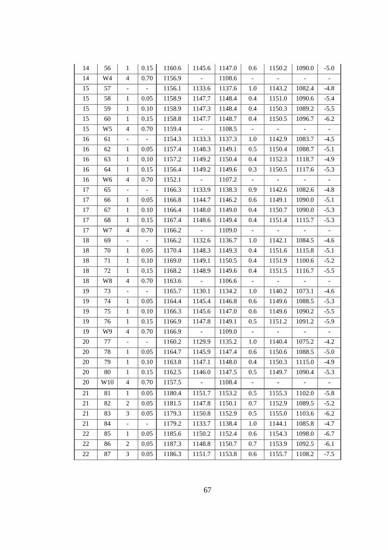
67

14 56 1 0.15 1160.6 1145.6 1147.0 0.6 1150.2 1090.0 -5.0

14 W4 4 0.70 1156.9 - 1108.6 - - - -

15 57 - - 1156.1 1133.6 1137.6 1.0 1143.2 1082.4 -4.8

15 58 1 0.05 1158.9 1147.7 1148.4 0.4 1151.0 1090.6 -5.4

15 59 1 0.10 1158.9 1147.3 1148.4 0.4 1150.3 1089.2 -5.5

15 60 1 0.15 1158.8 1147.7 1148.7 0.4 1150.5 1096.7 -6.2

15 W5 4 0.70 1159.4 - 1108.5 - - - -

16 61 - - 1154.3 1133.3 1137.3 1.0 1142.9 1083.7 -4.5

16 62 1 0.05 1157.4 1148.3 1149.1 0.5 1150.4 1088.7 -5.1

16 63 1 0.10 1157.2 1149.2 1150.4 0.4 1152.3 1118.7 -4.9

16 64 1 0.15 1156.4 1149.2 1149.6 0.3 1150.5 1117.6 -5.3

16 W6 4 0.70 1152.1 - 1107.2 - - - -

17 65 - - 1166.3 1133.9 1138.3 0.9 1142.6 1082.6 -4.8

17 66 1 0.05 1166.8 1144.7 1146.2 0.6 1149.1 1090.0 -5.1

17 67 1 0.10 1166.4 1148.0 1149.0 0.4 1150.7 1090.0 -5.3

17 68 1 0.15 1167.4 1148.6 1149.4 0.4 1151.4 1115.7 -5.3

17 W7 4 0.70 1166.2 - 1109.0 - - - -

18 69 - - 1166.2 1132.6 1136.7 1.0 1142.1 1084.5 -4.6

18 70 1 0.05 1170.4 1148.3 1149.3 0.4 1151.6 1115.8 -5.1

18 71 1 0.10 1169.0 1149.1 1150.5 0.4 1151.9 1100.6 -5.2

18 72 1 0.15 1168.2 1148.9 1149.6 0.4 1151.5 1116.7 -5.5

18 W8 4 0.70 1163.6 - 1106.6 - - - -

19 73 - - 1165.7 1130.1 1134.2 1.0 1140.2 1073.1 -4.6

19 74 1 0.05 1164.4 1145.4 1146.8 0.6 1149.6 1088.5 -5.3

19 75 1 0.10 1166.3 1145.6 1147.0 0.6 1149.6 1090.2 -5.5

19 76 1 0.15 1166.9 1147.8 1149.1 0.5 1151.2 1091.2 -5.9

19 W9 4 0.70 1166.9 - 1109.0 - - - -

20 77 - - 1160.2 1129.9 1135.2 1.0 1140.4 1075.2 -4.2

20 78 1 0.05 1164.7 1145.9 1147.4 0.6 1150.6 1088.5 -5.0

20 79 1 0.10 1163.8 1147.1 1148.0 0.4 1150.3 1115.0 -4.9

20 80 1 0.15 1162.5 1146.0 1147.5 0.5 1149.7 1090.4 -5.3

20 W10 4 0.70 1157.5 - 1108.4 - - - -

21 81 1 0.05 1180.4 1151.7 1153.2 0.5 1155.3 1102.0 -5.8

21 82 2 0.05 1181.5 1147.8 1150.1 0.7 1152.9 1089.5 -5.2

21 83 3 0.05 1179.3 1150.8 1152.9 0.5 1155.0 1103.6 -6.2

21 84 - - 1179.2 1133.7 1138.4 1.0 1144.1 1085.8 -4.7

22 85 1 0.05 1185.6 1150.2 1152.4 0.6 1154.3 1098.0 -6.7

22 86 2 0.05 1187.3 1148.8 1150.7 0.7 1153.9 1092.5 -6.1

22 87 3 0.05 1186.3 1151.7 1153.8 0.6 1155.7 1108.2 -7.5

68

22 88 - - 1185.8 1138.6 1142.0 0.9 1147.0 1090.3 -5.1

23 89 1 0.05 1180.8 1149.3 1151.5 0.7 1154.0 1098.0 -6.2

23 90 2 0.05 1181.8 1146.5 1148.9 0.8 1152.8 1095.7 -5.8

23 91 3 0.05 1181.9 1147.3 1149.5 0.8 1152.6 1097.4 -7.1

23 92 - - 1180.7 1135.2 1139.3 1.3 1146.0 1087.7 -5.4

24 93 1 0.05 1183.5 1148.5 1151.0 0.7 1154.4 1101.6 -5.2

24 94 2 0.05 1184.4 1146.8 1148.8 0.7 1152.4 1090.2 -5.2

24 95 3 0.05 1184.0 1150.6 1152.3 0.5 1154.3 1098.7 -5.8

24 96 - - 1183.4 1131.4 1136.7 1.3 1144.4 1090.4 -4.9

25 97 1 0.05 1185.0 1150.1 1151.7 0.7 1154.9 1105.5 -6.1

25 98 2 0.05 1186.0 1145.4 1147.6 0.7 1150.6 1086.9 -5.6

25 99 3 0.05 1185.8 1149.0 1151.2 0.7 1154.0 1102.5 -6.1

25 100 - - 1184.6 1130.3 1135.2 1.4 1141.9 1086.3 -5.7

26 101 1 0.05 1186.7 1150.2 1151.9 0.6 1154.4 1096.8 -5.5

26 102 2 0.05 1187.1 1144.2 1146.6 0.7 1150.2 1087.8 -5.1

26 103 3 0.05 1186.9 1149.3 1151.3 0.7 1154.4 1099.6 -5.4

26 104 - - 1184.8 1125.9 1132.0 1.4 1138.7 1078.8 -5.0

27 105 1 0.05 1183.9 1144.8 1147.5 0.9 1151.0 1090.9 -6.1

27 106 2 0.05 1184.9 1142.2 1144.9 0.9 1149.0 1086.1 -5.8

27 107 3 0.05 1184.0 1149.7 1152.3 0.7 1154.4 1101.7 -6.2

27 108 - - 1183.1 1129.7 1135.6 1.4 1142.6 1087.2 -5.1

28 109 1 0.05 1184.2 1148.6 1150.7 0.7 1153.9 1096.2 -5.2

28 110 2 0.05 1185.1 1145.5 1146.9 0.6 1149.5 1083.0 -5.1

28 111 3 0.05 1184.7 1146.6 1149.4 0.9 1153.3 1102.1 -6.1

28 112 - - 1183.7 1129.3 1134.2 1.5 1141.8 1084.2 -5.4

29 113 1 0.05 1175.4 1150.2 1152.0 0.5 1154.1 1104.0 -6.0

29 114 2 0.05 1176.0 1146.7 1149.3 0.8 1153.0 1099.5 -5.6

29 115 3 0.05 1174.3 1147.8 1150.0 0.8 1153.4 1093.0 -6.3

29 116 - - 1174.2 1133.1 1138.7 1.5 1145.9 1092.9 -6.0

30 117 1 0.05 1176.7 1150.5 1152.0 0.5 1154.3 1092.6 -5.6

30 118 2 0.05 1176.9 1141.9 1144.0 0.7 1147.4 1080.8 -5.0

30 119 3 0.05 1176.0 1149.6 1151.6 0.7 1154.2 1093.5 -5.3

30 120 - - 1176.0 1125.9 1133.1 1.5 1140.5 1083.8 -4.8

31 121 - - 1181.3 1133.5 1137.8 1.1 1142.9 1084.0 -5.1

31 122 1 0.05 1183.3 1149.3 1150.9 0.6 1153.2 1089.8 -5.4

31 123 1 0.10 1184.1 1144.8 1147.0 0.6 1149.2 1087.8 -5.2

31 124 1 0.15 1183.0 1150.1 1151.7 0.5 1153.7 1092.8 -5.7

31 W11 4 0.70 1183.8 - 1074.3 - - - -

32 125 - - 1179.9 1134.8 1138.5 1.0 1143.5 1084.4 -5.1

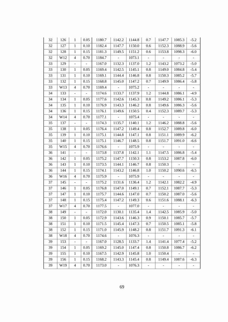
69

32 126 1 0.05 1180.7 1142.2 1144.8 0.7 1147.7 1085.3 -5.2

32 127 1 0.10 1182.4 1147.7 1150.0 0.6 1152.3 1088.9 -5.6

32 128 1 0.15 1181.3 1149.5 1151.2 0.6 1153.8 1098.3 -6.0

32 W12 4 0.70 1184.7 - 1073.1 - - - -

33 129 - - 1167.0 1132.3 1137.0 1.2 1143.2 1073.2 -5.0

33 130 1 0.05 1169.4 1142.5 1145.1 0.8 1149.0 1084.8 -5.4

33 131 1 0.10 1169.1 1144.4 1146.8 0.8 1150.3 1085.2 -5.7

33 132 1 0.15 1168.8 1145.0 1147.2 0.7 1149.9 1086.4 -5.8

33 W13 4 0.70 1169.4 - 1075.2 - - - -

34 133 - - 1174.6 1133.7 1137.9 1.2 1144.8 1086.1 -4.9

34 134 1 0.05 1177.6 1142.6 1145.3 0.8 1149.2 1086.1 -5.3

34 135 1 0.10 1176.9 1143.3 1146.2 0.8 1149.6 1086.3 -5.6

34 136 1 0.15 1176.1 1149.6 1150.5 0.4 1152.3 1089.7 -5.3

34 W14 4 0.70 1177.1 - 1075.4 - - - -

35 137 - - 1174.3 1135.7 1140.1 1.2 1146.2 1088.8 -5.6

35 138 1 0.05 1176.4 1147.2 1149.4 0.8 1152.7 1089.8 -6.0

35 139 1 0.10 1175.1 1144.8 1147.1 0.8 1151.1 1089.9 -6.2

35 140 1 0.15 1175.1 1146.7 1148.5 0.8 1151.7 1091.0 -6.6

35 W15 4 0.70 1176.6 - 1075.9 - - - -

36 141 - - 1173.8 1137.8 1142.1 1.1 1147.5 1086.8 -5.4

36 142 1 0.05 1175.2 1147.7 1150.3 0.8 1153.2 1087.8 -6.0

36 143 1 0.10 1173.5 1144.1 1146.7 0.8 1150.3 - -

36 144 1 0.15 1174.1 1143.2 1146.8 1.0 1150.2 1090.6 -6.5

36 W16 4 0.70 1175.9 - 1075.9 - - - -

37 145 - - 1175.2 1131.6 1136.4 1.2 1142.1 1082.2 -4.9

37 146 1 0.05 1176.8 1147.0 1149.1 0.7 1152.1 1087.7 -5.3

37 147 1 0.10 1175.7 1144.6 1147.0 0.7 1150.2 1087.0 -5.6

37 148 1 0.15 1175.4 1147.2 1149.3 0.6 1151.6 1088.1 -6.3

37 W17 4 0.70 1177.5 - 1077.0 - - - -

38 149 - - 1172.0 1130.1 1135.4 1.4 1142.5 1085.9 -5.0

38 150 1 0.05 1172.9 1143.6 1146.3 0.9 1150.1 1085.7 -5.7

38 151 1 0.10 1171.5 1145.4 1147.3 0.7 1150.5 1085.1 -5.8

38 152 1 0.15 1171.0 1145.9 1148.2 0.8 1151.7 1091.3 -6.1

38 W18 4 0.70 1174.6 - 1076.3 - - - -

39 153 - - 1167.0 1128.5 1133.7 1.4 1141.4 1077.4 -5.2

39 154 1 0.05 1169.2 1145.0 1147.4 0.8 1150.8 1086.7 -6.2

39 155 1 0.10 1167.5 1142.9 1145.8 1.0 1150.4 - -

39 156 1 0.15 1168.2 1143.3 1145.4 0.8 1149.4 1087.6 -6.3

39 W19 4 0.70 1173.0 - 1076.3 - - - -

70

40 157 - - 1173.9 1128.1 1137.7 1.2 1143.8 1083.2 -5.1

40 158 1 0.05 1175.7 1147.4 1147.6 0.8 1150.9 1087.1 -5.6

40 159 1 0.10 1175.1 1148.4 1147.1 0.8 1150.4 1087.2 -5.7

40 160 1 0.15 1174.8 1148.6 1148.8 0.7 1151.6 1090.6 -6.1

40 W20 4 0.70 1176.9 - 1075.6 - - - -

Liquidus temperature (TL) versus alloy grade chart is revealed in Figure 4.2 as box

chart. In hypoeutectic part of Fe-C binary phase diagram, liquidus temperature is the

temperature at which pro-eutectic austenite dendrites nucleate and start growing, and

it is dependent on the carbon content or in this (cast iron) case carbon equivalent. As

can be seen in Figure 4.2, in general, the specimens of EN-GJS-600-10C grade have

a higher liquidus temperature than that the ones of EN-GJS-400-18 do. Average

liquidus temperature difference among two alloys is 15.0oC. When the average carbon

equivalent difference among two alloys is calculated according to Equation 2.1, the

specimens of EN-GJS-400-18 have 0.04% higher average carbon equivalent, and

according to Equation 2.2, it is 0.17%. If we assume that slope of the hypoeutectic

liquidus line is -91.6oC / %C.E., 15.0oC change in liquidus temperature requires 0.16%

of change in carbon equivalent. Therefore, it is possible to say that Equation 2.2 gives

a good estimation for the effect of silicon on the hypoeutectic liquidus line of Fe-C

phase diagram.

71

Figure 4.2. Liquidus temperature (TL) versus alloy grade.

Upper eutectic temperature (TEmax) versus alloy grade chart is revealed for plain and

inoculated analysis cups separately in Figure 4.3 as box chart. Upper eutectic

temperature is the point at which the recalescence ends up, and the cooling down starts

back. Recalescence occurs due to heat evolved in a high rate as a result of high growth

rate of the graphite particles, thus high rate of carbon dissociation. Therefore, it starts

right after the nucleation of graphite particles which is represented by lower eutectic

temperature (TEmin), and if there are enough heterogeneous nucleation sites for

graphite, recalescence is limited by the stable eutectic transformation temperature

because a high amount of (latent) heat needs be produced to go above that temperature

or to melt back. If there are not enough heterogeneous nucleation sites for graphite,

recalescence is limited by the density of the growing graphite particles in the matrix

which defines the diffusion path. As can be seen in Figure 4.3, in general, for both

alloy grades, the specimens from plain analysis cups have lower TEmax values, and

EN-GJS-400-18 EN-GJS-600-10C

1150

1160

1170

1180

1190

TL (

°C)

72

TEmax values of the specimens from inoculant containing cups mostly accumulated

at top. This can be explained by that TEmax values of the specimens from plain cups

are limited by the low density of graphite particles making the carbon diffusion path

longer, and TEmax values of the ones from inoculant containing cups are limited by

the stable eutectic transformation temperature which requires re-melting to go beyond.

In Figure 4.3, it can also be seen that TEmax values of the EN-GJS-EN-400-18

specimens that are saturated in terms of heterogeneous nucleation sites are aligned at

around 1152oC which is the stable eutectic transformation temperature. On the other

hand, the ones of EN-GJS EN-GJS-600-10C are aligned at around 1154oC. This

difference can be explained by the effect of silicon on the eutectic transformation

temperatures such that it increases the stable eutectic transformation temperature

while decreasing the metastable one. Since EN-GJS-600-10C grade has a higher

silicon content, it is expected to have a higher stable eutectic transformation

temperature. It is difficult to define the magnitude of the effect of silicon on the stable

eutectic transformation temperature due to the variety of factors defining the diffusion

kinetics for particle growth.

73

Figure 4.3. Upper eutectic temperature (TEmax) versus alloy grade for plain and inoculated analysis

cups separately.

Time difference between the end of freezing (TF) and lower eutectic (TEmin) points

of the cooling curve (TF_t – TEmin_t) versus alloy grade chart is revealed in Figure

4.4 as box chart. In cooling curve of hypoeutectic ductile iron; after the liquidus,

temperature decreases until there is enough driving force for graphite particles to

nucleate and grow, so eutectic transformation starts at the lower eutectic point, then

the graphite growth rate is so high that the heat evolved is higher than the heat removed

by the surroundings, and temperature increases until the upper eutectic point, then it

starts cooling back but not as fast because the growth slowly continues until the end

of freezing point where the cooling rate increases since the growth terminated, thus

the eutectic transformation. Therefore, it is possible to say that growth of the graphite

particles or the eutectic transformation starts around the lower eutectic point, and ends

around the end of freezing point, so the time difference between these two points gives

an idea on the total duration of graphite growth or eutectic transformation. As can be

seen in Figure 4.4, in general, the specimens of EN-GJS-600-10C grade have a lower

time difference between the end of freezing and the lower eutectic points than that the

ones of EN-GJS-400-18 do. This can be explained by that the specimens of EN-GJS-

600-10C grade have less amount of graphite in their microstructure (see Figure 4.7),

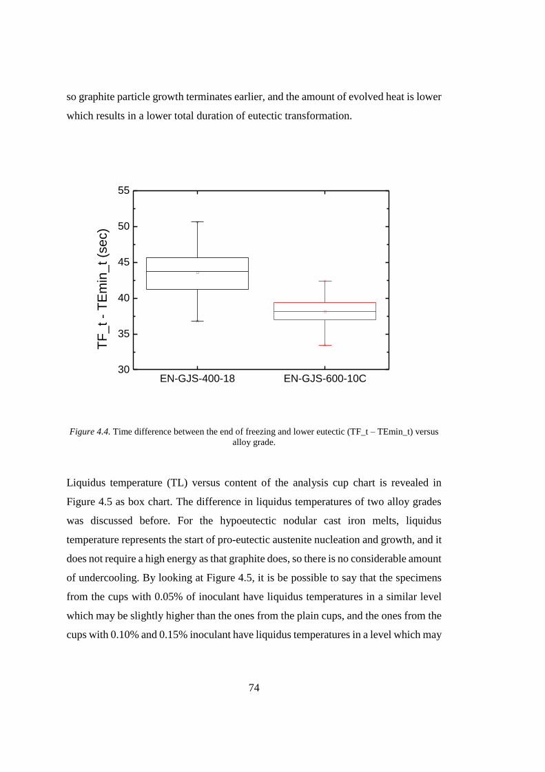
74

so graphite particle growth terminates earlier, and the amount of evolved heat is lower

which results in a lower total duration of eutectic transformation.

EN-GJS-400-18 EN-GJS-600-10C30

35

40

45

50

55

TF

_t -

TE

min

_t (s

ec)

Figure 4.4. Time difference between the end of freezing and lower eutectic (TF_t – TEmin_t) versus

alloy grade.

Liquidus temperature (TL) versus content of the analysis cup chart is revealed in

Figure 4.5 as box chart. The difference in liquidus temperatures of two alloy grades

was discussed before. For the hypoeutectic nodular cast iron melts, liquidus

temperature represents the start of pro-eutectic austenite nucleation and growth, and it

does not require a high energy as that graphite does, so there is no considerable amount

of undercooling. By looking at Figure 4.5, it is be possible to say that the specimens

from the cups with 0.05% of inoculant have liquidus temperatures in a similar level

which may be slightly higher than the ones from the plain cups, and the ones from the

cups with 0.10% and 0.15% inoculant have liquidus temperatures in a level which may

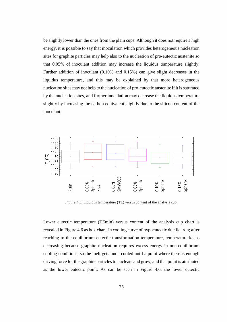
75

be slightly lower than the ones from the plain cups. Although it does not require a high

energy, it is possible to say that inoculation which provides heterogeneous nucleation

sites for graphite particles may help also to the nucleation of pro-eutectic austenite so

that 0.05% of inoculant addition may increase the liquidus temperature slightly.

Further addition of inoculant (0.10% and 0.15%) can give slight decreases in the

liquidus temperature, and this may be explained by that more heterogeneous

nucleation sites may not help to the nucleation of pro-eutectic austenite if it is saturated

by the nucleation sites, and further inoculation may decrease the liquidus temperature

slightly by increasing the carbon equivalent slightly due to the silicon content of the

inoculant.

Figure 4.5. Liquidus temperature (TL) versus content of the analysis cup.

Lower eutectic temperature (TEmin) versus content of the analysis cup chart is

revealed in Figure 4.6 as box chart. In cooling curve of hypoeutectic ductile iron; after

reaching to the equilibrium eutectic transformation temperature, temperature keeps

decreasing because graphite nucleation requires excess energy in non-equilibrium

cooling conditions, so the melt gets undercooled until a point where there is enough

driving force for the graphite particles to nucleate and grow, and that point is attributed

as the lower eutectic point. As can be seen in Figure 4.6, the lower eutectic

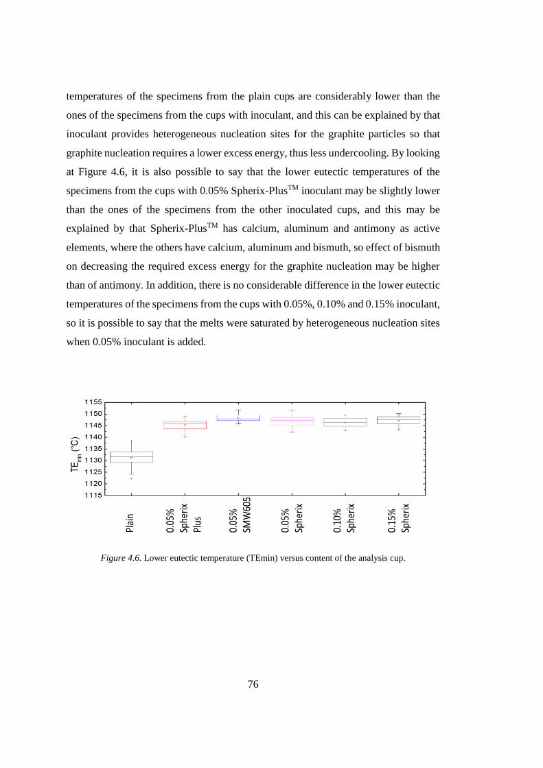
76

temperatures of the specimens from the plain cups are considerably lower than the

ones of the specimens from the cups with inoculant, and this can be explained by that

inoculant provides heterogeneous nucleation sites for the graphite particles so that

graphite nucleation requires a lower excess energy, thus less undercooling. By looking

at Figure 4.6, it is also possible to say that the lower eutectic temperatures of the

specimens from the cups with 0.05% Spherix-PlusTM inoculant may be slightly lower

than the ones of the specimens from the other inoculated cups, and this may be

explained by that Spherix-PlusTM has calcium, aluminum and antimony as active

elements, where the others have calcium, aluminum and bismuth, so effect of bismuth

on decreasing the required excess energy for the graphite nucleation may be higher

than of antimony. In addition, there is no considerable difference in the lower eutectic

temperatures of the specimens from the cups with 0.05%, 0.10% and 0.15% inoculant,

so it is possible to say that the melts were saturated by heterogeneous nucleation sites

when 0.05% inoculant is added.

Figure 4.6. Lower eutectic temperature (TEmin) versus content of the analysis cup.

77

4.4. Metallographic Image Analysis

The main results obtained from the metallographic evaluation of the thermal analysis

cup samples by using an image analysis software are listed in Table 4.4.

Table 4.4. The main results of metallographic image analysis indicating contents of the analysis cups

(Content types; 1-SpherixTM inoculant, 2-Sperix-PlusTM inoculant, 3-SMW605TM inoculant, 4-Te and

S).

Ladle Cup Content Graphite Nodule Count Nodularity Pearlite Ferrite

# # Type % % 1/mm2 % % %

1 1 1 0.05 10.0 819.2 64.2 5.4 94.6

1 2 2 0.05 12.2 717.9 71.9 9.2 90.8

1 3 3 0.05 11.5 971.5 65.4 8.8 91.2

1 4 - - 12.4 416.9 75.8 28.6 71.4

2 5 1 0.05 13.2 811.9 65.3 4.8 95.2

2 6 2 0.05 12.5 612.3 76.7 17.0 83.0

2 7 3 0.05 10.9 849.2 64.3 16.1 83.9

2 8 - - 10.5 452.4 71.5 38.7 61.3

3 9 1 0.05 10.1 600.3 74.6 22.2 77.8

3 10 2 0.05 8.8 697.4 70.6 17.9 82.1

3 11 3 0.05 8.8 699.6 69.9 19.7 80.3

3 12 - - 9.6 392.5 72.7 38.3 61.7

4 13 1 0.05 10.2 767.5 68.5 17.1 82.9

4 14 2 0.05 9.1 571.3 73.1 22.1 77.9

4 15 3 0.05 8.7 680.4 67.3 16.5 83.5

4 16 - - 9.6 206.0 73.9 49.7 50.3

5 17 1 0.05 9.7 694.9 70.4 24.2 75.8

5 18 2 0.05 8.3 590.6 65.6 18.5 81.5

5 19 3 0.05 8.0 670.1 65.5 14.6 85.4

5 20 - - 10.4 433.7 75.3 36.5 63.5

6 21 1 0.05 8.4 706.6 66.2 11.8 88.2

6 22 2 0.05 11.4 540.9 73.8 9.5 90.5

6 23 3 0.05 11.9 829.4 65.7 8.2 91.8

6 24 - - 11.4 401.1 79.0 45.0 55.0

7 25 1 0.05 11.6 779.8 71.5 8.6 91.4

7 26 2 0.05 10.7 516.4 75.4 24.4 75.6

7 27 3 0.05 9.3 756.0 69.9 11.9 88.1

7 28 - - 10.2 399.5 75.7 37.6 62.4

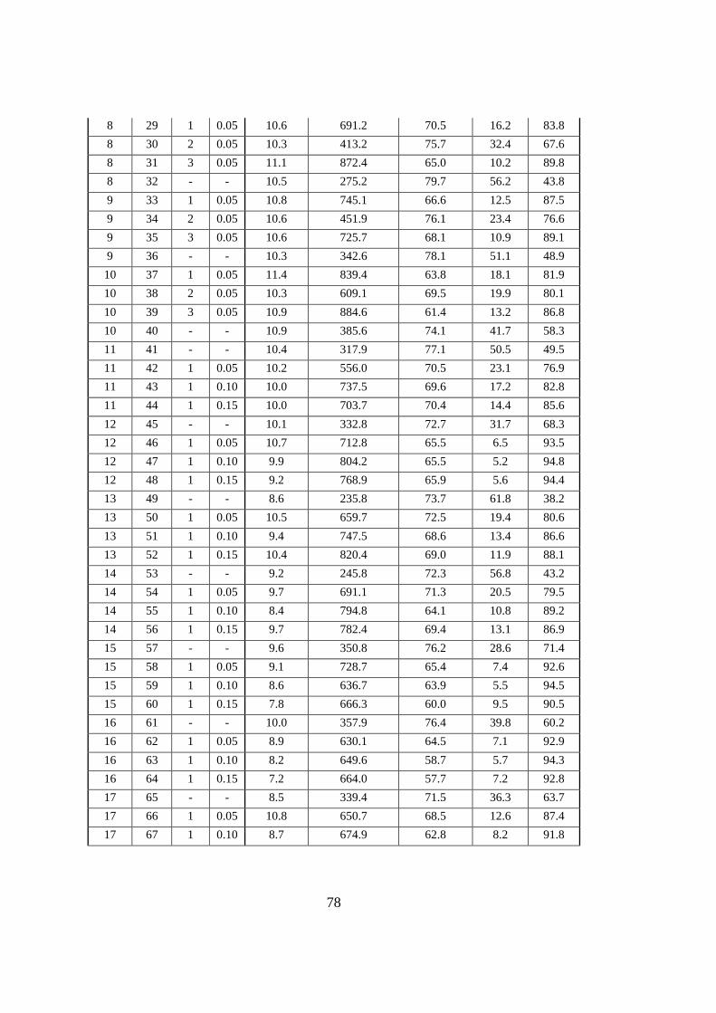
78

8 29 1 0.05 10.6 691.2 70.5 16.2 83.8

8 30 2 0.05 10.3 413.2 75.7 32.4 67.6

8 31 3 0.05 11.1 872.4 65.0 10.2 89.8

8 32 - - 10.5 275.2 79.7 56.2 43.8

9 33 1 0.05 10.8 745.1 66.6 12.5 87.5

9 34 2 0.05 10.6 451.9 76.1 23.4 76.6

9 35 3 0.05 10.6 725.7 68.1 10.9 89.1

9 36 - - 10.3 342.6 78.1 51.1 48.9

10 37 1 0.05 11.4 839.4 63.8 18.1 81.9

10 38 2 0.05 10.3 609.1 69.5 19.9 80.1

10 39 3 0.05 10.9 884.6 61.4 13.2 86.8

10 40 - - 10.9 385.6 74.1 41.7 58.3

11 41 - - 10.4 317.9 77.1 50.5 49.5

11 42 1 0.05 10.2 556.0 70.5 23.1 76.9

11 43 1 0.10 10.0 737.5 69.6 17.2 82.8

11 44 1 0.15 10.0 703.7 70.4 14.4 85.6

12 45 - - 10.1 332.8 72.7 31.7 68.3

12 46 1 0.05 10.7 712.8 65.5 6.5 93.5

12 47 1 0.10 9.9 804.2 65.5 5.2 94.8

12 48 1 0.15 9.2 768.9 65.9 5.6 94.4

13 49 - - 8.6 235.8 73.7 61.8 38.2

13 50 1 0.05 10.5 659.7 72.5 19.4 80.6

13 51 1 0.10 9.4 747.5 68.6 13.4 86.6

13 52 1 0.15 10.4 820.4 69.0 11.9 88.1

14 53 - - 9.2 245.8 72.3 56.8 43.2

14 54 1 0.05 9.7 691.1 71.3 20.5 79.5

14 55 1 0.10 8.4 794.8 64.1 10.8 89.2

14 56 1 0.15 9.7 782.4 69.4 13.1 86.9

15 57 - - 9.6 350.8 76.2 28.6 71.4

15 58 1 0.05 9.1 728.7 65.4 7.4 92.6

15 59 1 0.10 8.6 636.7 63.9 5.5 94.5

15 60 1 0.15 7.8 666.3 60.0 9.5 90.5

16 61 - - 10.0 357.9 76.4 39.8 60.2

16 62 1 0.05 8.9 630.1 64.5 7.1 92.9

16 63 1 0.10 8.2 649.6 58.7 5.7 94.3

16 64 1 0.15 7.2 664.0 57.7 7.2 92.8

17 65 - - 8.5 339.4 71.5 36.3 63.7

17 66 1 0.05 10.8 650.7 68.5 12.6 87.4

17 67 1 0.10 8.7 674.9 62.8 8.2 91.8

79

17 68 1 0.15 9.1 745.1 60.2 2.9 97.1

18 69 - - 9.4 346.7 75.4 35.6 64.4

18 70 1 0.05 9.6 735.0 67.3 4.6 95.4

18 71 1 0.10 9.6 814.3 65.2 3.1 96.9

18 72 1 0.15 8.6 767.5 63.1 4.1 95.9

19 73 - - 10.5 343.5 79.0 49.0 51.0

19 74 1 0.05 11.7 641.2 72.7 20.2 79.8

19 75 1 0.10 11.8 721.5 71.7 15.8 84.2

19 76 1 0.15 9.9 775.8 66.3 8.0 92.0

20 77 - - 10.9 345.6 78.1 30.7 69.3

20 78 1 0.05 12.3 664.7 73.0 7.1 92.9

20 79 1 0.10 9.7 810.7 66.6 7.0 93.0

20 80 1 0.15 9.8 810.0 66.5 4.6 95.4

21 81 1 0.05 6.8 637.7 58.0 5.0 95.0

21 82 2 0.05 8.0 536.6 66.6 2.4 97.6

21 83 3 0.05 8.3 710.3 57.8 4.7 95.3

21 84 - - 8.3 435.2 72.2 1.8 98.2

22 85 1 0.05 11.2 768.3 63.5 0.4 99.6

22 86 2 0.05 10.9 638.3 68.5 2.5 97.5

22 87 3 0.05 8.6 711.8 62.0 5.2 94.8

22 88 - - 6.5 435.8 69.8 4.5 95.5

23 89 1 0.05 9.6 758.7 67.5 0.0 100.0

23 90 2 0.05 9.7 608.7 69.1 3.6 96.4

23 91 3 0.05 9.1 789.1 65.3 5.0 95.0

23 92 - - 5.7 426.4 67.3 2.8 97.2

24 93 1 0.05 9.7 669.0 67.1 0.0 100.0

24 94 2 0.05 9.5 547.6 70.2 0.0 100.0

24 95 3 0.05 10.7 864.0 63.3 0.0 100.0

24 96 - - 6.4 387.1 70.9 3.9 96.1

25 97 1 0.05 10.9 812.7 62.3 0.0 100.0

25 98 2 0.05 9.8 535.5 75.3 2.0 98.0

25 99 3 0.05 9.8 753.7 66.4 1.0 99.0

25 100 - - 6.2 410.7 72.4 3.9 96.1

26 101 1 0.05 9.6 830.5 60.4 0.3 99.7

26 102 2 0.05 9.5 501.7 74.3 1.9 98.1

26 103 3 0.05 11.5 846.9 59.3 0.0 100.0

26 104 - - 6.6 310.3 70.2 5.4 94.6

27 105 1 0.05 9.4 637.2 71.5 0.7 99.3

27 106 2 0.05 9.7 520.8 77.8 0.4 99.6

80

27 107 3 0.05 9.6 867.9 63.4 0.0 100.0

27 108 - - 6.6 416.5 68.2 4.4 95.6

28 109 1 0.05 9.5 695.9 68.5 1.8 98.2

28 110 2 0.05 9.3 546.6 73.7 2.8 97.2

28 111 3 0.05 9.4 683.5 68.1 2.9 97.1

28 112 - - 7.2 402.8 74.7 2.7 97.3

29 113 1 0.05 9.7 789.1 66.7 0.7 99.3

29 114 2 0.05 9.6 540.0 77.2 1.6 98.4

29 115 3 0.05 9.6 791.6 66.0 2.0 98.0

29 116 - - 6.8 384.1 70.5 4.6 95.4

30 117 1 0.05 10.6 902.7 60.4 0.9 99.1

30 118 2 0.05 10.3 460.0 77.1 2.2 97.8

30 119 3 0.05 9.2 860.7 58.0 0.3 99.7

30 120 - - 7.0 283.1 72.5 6.1 93.9

31 121 - - 6.3 380.2 68.4 5.6 94.4

31 122 1 0.05 5.1 523.5 62.4 3.7 96.3

31 123 1 0.10 5.5 448.0 63.9 3.0 97.0

31 124 1 0.15 6.4 631.4 65.0 2.9 97.1

32 125 - - 6.5 371.1 70.1 5.4 94.6

32 126 1 0.05 7.0 468.8 70.0 2.8 97.2

32 127 1 0.10 5.4 518.7 66.1 3.1 96.9

32 128 1 0.15 4.9 525.8 61.1 3.7 96.3

33 129 - - 6.4 349.4 69.8 6.0 94.0

33 130 1 0.05 7.4 458.9 75.9 3.1 96.9

33 131 1 0.10 6.5 503.1 72.2 3.0 97.0

33 132 1 0.15 7.1 563.0 73.3 2.7 97.3

34 133 - - 7.5 402.4 73.5 4.3 95.7

34 134 1 0.05 6.8 468.3 74.1 3.7 96.3

34 135 1 0.10 6.3 475.0 70.4 4.1 95.9

34 136 1 0.15 6.4 637.6 68.6 3.5 96.5

35 137 - - 6.7 432.1 71.0 2.8 97.2

35 138 1 0.05 5.8 484.5 65.6 2.2 97.8

35 139 1 0.10 5.3 467.5 66.8 3.1 96.9

35 140 1 0.15 5.8 537.9 69.1 3.5 96.5

36 141 - - 6.4 451.5 71.1 2.0 98.0

36 142 1 0.05 5.8 529.5 68.7 2.4 97.6

36 143 1 0.10 6.8 521.4 73.8 3.0 97.0

36 144 1 0.15 7.6 540.0 75.4 2.3 97.7

37 145 - - 7.0 373.4 75.2 4.1 95.9

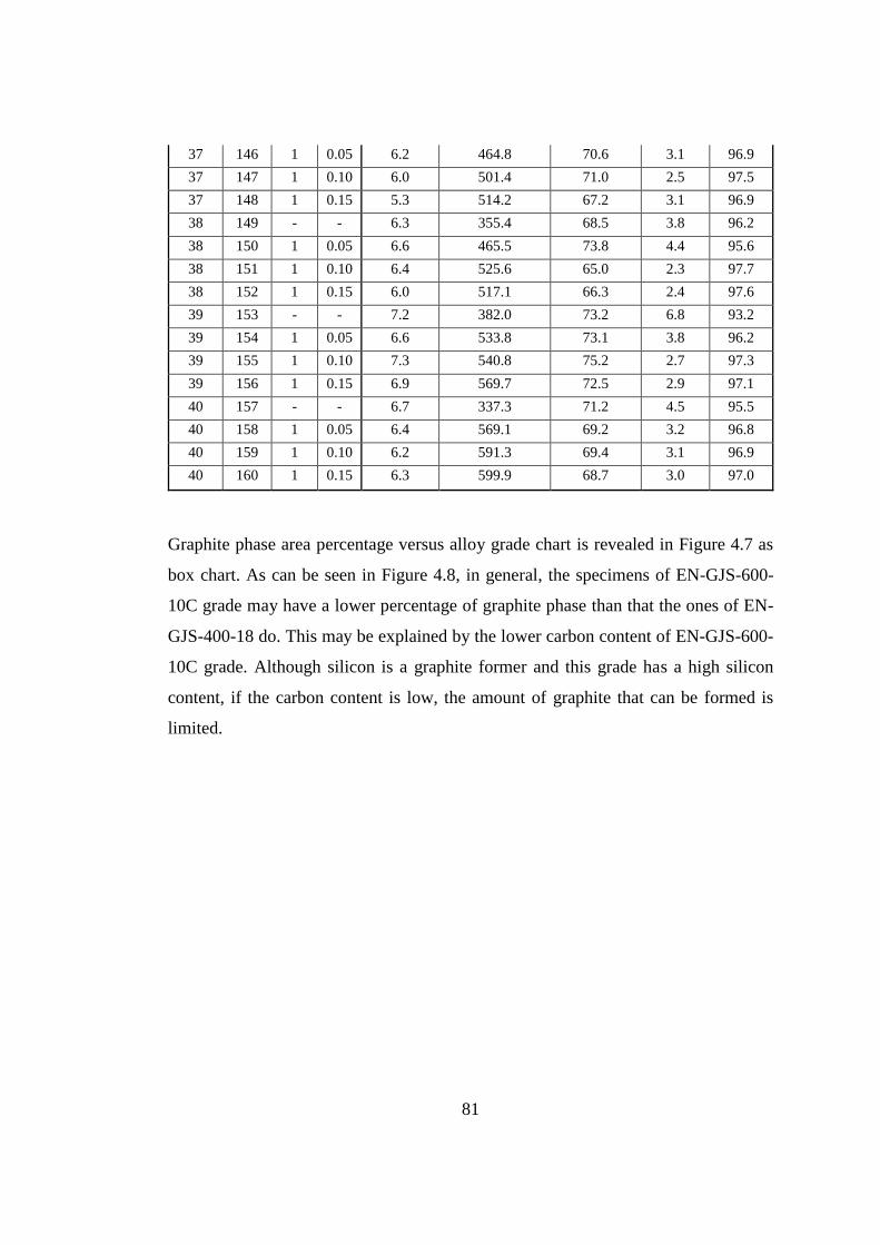
81

37 146 1 0.05 6.2 464.8 70.6 3.1 96.9

37 147 1 0.10 6.0 501.4 71.0 2.5 97.5

37 148 1 0.15 5.3 514.2 67.2 3.1 96.9

38 149 - - 6.3 355.4 68.5 3.8 96.2

38 150 1 0.05 6.6 465.5 73.8 4.4 95.6

38 151 1 0.10 6.4 525.6 65.0 2.3 97.7

38 152 1 0.15 6.0 517.1 66.3 2.4 97.6

39 153 - - 7.2 382.0 73.2 6.8 93.2

39 154 1 0.05 6.6 533.8 73.1 3.8 96.2

39 155 1 0.10 7.3 540.8 75.2 2.7 97.3

39 156 1 0.15 6.9 569.7 72.5 2.9 97.1

40 157 - - 6.7 337.3 71.2 4.5 95.5

40 158 1 0.05 6.4 569.1 69.2 3.2 96.8

40 159 1 0.10 6.2 591.3 69.4 3.1 96.9

40 160 1 0.15 6.3 599.9 68.7 3.0 97.0

Graphite phase area percentage versus alloy grade chart is revealed in Figure 4.7 as

box chart. As can be seen in Figure 4.8, in general, the specimens of EN-GJS-600-

10C grade may have a lower percentage of graphite phase than that the ones of EN-

GJS-400-18 do. This may be explained by the lower carbon content of EN-GJS-600-

10C grade. Although silicon is a graphite former and this grade has a high silicon

content, if the carbon content is low, the amount of graphite that can be formed is

limited.

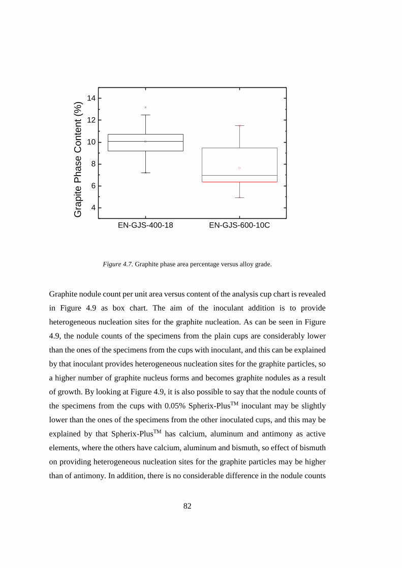
82

EN-GJS-400-18 EN-GJS-600-10C

4

6

8

10

12

14

Gra

pite P

hase C

onte

nt (%

)

Figure 4.7. Graphite phase area percentage versus alloy grade.

Graphite nodule count per unit area versus content of the analysis cup chart is revealed

in Figure 4.9 as box chart. The aim of the inoculant addition is to provide

heterogeneous nucleation sites for the graphite nucleation. As can be seen in Figure

4.9, the nodule counts of the specimens from the plain cups are considerably lower

than the ones of the specimens from the cups with inoculant, and this can be explained

by that inoculant provides heterogeneous nucleation sites for the graphite particles, so

a higher number of graphite nucleus forms and becomes graphite nodules as a result

of growth. By looking at Figure 4.9, it is also possible to say that the nodule counts of

the specimens from the cups with 0.05% Spherix-PlusTM inoculant may be slightly

lower than the ones of the specimens from the other inoculated cups, and this may be

explained by that Spherix-PlusTM has calcium, aluminum and antimony as active

elements, where the others have calcium, aluminum and bismuth, so effect of bismuth

on providing heterogeneous nucleation sites for the graphite particles may be higher

than of antimony. In addition, there is no considerable difference in the nodule counts

83

of the specimens from the cups with 0.05%, 0.10% and 0.15% SpherixTM inoculant,

but the ones from the cups with 0.05% SMW605 inoculant may have slightly higher

nodule counts. Therefore, it is possible to say that the melts were saturated by

heterogeneous nucleation sites when 0.05% inoculant is added, and SMW605

inoculant may increase the nodule count slightly more than that SpherixTM inoculant

does which may be a result of higher calcium and rare earth metals content of

SMW605TM (see Table 3.4).

Figure 4.8. Graphite nodule count per unit area versus content of the analysis cup.

Graphite shape nodularity percentage versus content of the analysis cup chart is

revealed in Figure 4.10 as box chart. By the magnesium treatment, content of the

surface-active elements (oxygen and sulphur) reduces, and this increases the interface

energy between graphite and iron which makes increasing the volume/surface-area

ratio of the graphite particles thermodynamically more feasible, so it makes the high

nodularity graphite shape more stable. According to the solidification model

suggested by J. Zhou et al., when the diameter of graphite nodule exceeds a certain

value, it gets surrounded by austenite dendrite arms terminating its contact with liquid

phase, and that limits further growth of graphite nodule by the limited rate of solid

state diffusion [26]. In addition, since during the austenite envelopment, the parts of

84

the graphite nodule which have not been enveloped will be in contact with liquid and

will grow much faster than the enveloped parts due to the much higher diffusion rate,

the speed that graphite nodule gets enveloped by austenite has a significant effect on

the graphite shape [26]. Therefore, it is possible to say that content of the surface-

active elements defines the thermodynamic feasibility of high nodularity graphite

shape, where the speed that graphite nodule gets enveloped by austenite defines the

kinetic limitation of it. As can be seen in Figure 4.10, the nodularity of the specimens

from the plain cups is higher than the nodularity of the specimens from the cups with

inoculant. While inoculant master alloys are creating heterogeneous nucleation sites,

they bond oxygen and sulphur chemically, so content of the surface-active elements

decreases further, and thermodynamic stability of high nodularity increases further.

Therefore, it is expected the inoculants to have a positive effect on the nodularity

which is the opposite of the observed effect. On the other hand, if we consider the

kinetic factors, J. Zhou et al. claims that bismuth and antimony are two of the elements

that favor the slower envelopment of graphite by decreasing the growth rate of

austenite dendrites [26]. Since the inoculants that were used contain either bismuth or

antimony, the negative effect on the nodularity may be explained by this kinetic

limitation. By looking at Figure 4.10, it is also possible to say that the nodularity of

the specimens from the cups with 0.05% Spherix-PlusTM inoculant is slightly higher

than the nodularity of the specimens from the other inoculated cups. Although there

is no study found for such a comparison, this observation may indicate that bismuth

may have a higher effect on lowering the envelopment speed than that antimony does.

85

Figure 4.9. Graphite shape nodularity percentage versus content of the analysis cup.

4.5. Regression Analysis

Ferrite phase area percentage versus graphite nodule count per unit are graph is

revealed in Figure 4.11 as point scatter. Blue points indicate the cups with the alloy

EN-GJS-400-18, where the orange ones indicate the cups with the alloy EN-GJS-600-

10C. As can be seen in Figure 4.11, for both alloy grades, the ferrite content increases

when the nodule count increases, and this can be explained by that higher number of

graphite nodules per unit area decreases the length of the diffusion path of carbon

atoms to reach to the graphite phase, and this decreases the carbon content in the

matrix, thus the possibility to form pearlite. Equation and r-square value of the found

linear regression for the grade EN-GJS-400-18 are also revealed in Figure 4.11, and it

estimates around 7% increase in the ferrite content as the nodule count increases 100

1/mm2. For the grade EN-GJS-600-10C, there could not be found a considerable

correlation since its specimens have almost no pearlite.

86

Figure 4.10. Ferrite phase area percentage versus graphite nodule count per unit area graph indicating

the alloy grades and linear regression found for the grade EN-GJS-400-18.

87

The etched specimen micrographs at 100X magnification; from the ladle 2, sample

numbers a) 5 (with 0.05% SpherixTM) and b) 8 (Plain); from the ladle 6, sample

numbers c) 23 (with 0.05% SMW605TM) and d) 24 (Plain); from the ladle 9, sample

numbers e) 35 (with 0.05% SMW605TM) and f) 36 (Plain) were revealed in Figure

4.11. Since the samples from the same ladle have the similar chemical compositions

but different inoculation conditions, they can reveal the effect of graphite nodule count

per unit area on the ferrite phase content. A) sample 5 has 811.9 nodules per mm2 and

95.2% of ferrite content where b) sample 8 has 452.4 nodules per mm2 and 61.3% of

ferrite content; c) sample 23 has 829.4 nodules per mm2 and 91.8% of ferrite content

where d) sample 24 has 401.1 nodules per mm2 and 55.0% of ferrite content; e) sample

35 has 725.7 nodules per mm2 and 89.1% of ferrite content where f) sample 36 has

342.6 nodules per mm2 and 48.9% of ferrite content. It can be seen clearly in Figure

4.11 that as the graphite nodule count per unit area decreases, ferrite phase content

decreases too.

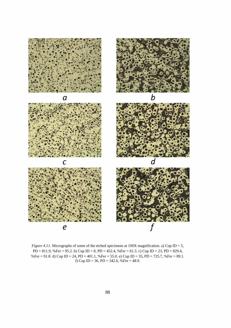
88

Figure 4.11. Micrographs of some of the etched specimens at 100X magnification. a) Cup ID = 5,

PD = 811.9, %Fer = 95.2. b) Cup ID = 8, PD = 452.4, %Fer = 61.3. c) Cup ID = 23, PD = 829.4,

%Fer = 91.8. d) Cup ID = 24, PD = 401.1, %Fer = 55.0. e) Cup ID = 35, PD = 725.7, %Fer = 89.1.

f) Cup ID = 36, PD = 342.6, %Fer = 48.9.

89

Since two alloy grades have a high difference in silicon content which affects both

stable and metastable eutectic transformation temperatures, the regression analysis

corresponding the eutectic part parameters of the cooling curves are conducted

separately for two grades.

Lower eutectic temperature (TEmin) and graphite nodule count per unit area are two

of the parameters expected to be related. Although there is a linear relationship

between those two parameters, it is not valid for the higher TEmin values due to the

saturation. Therefore, applying a non-linear fit could make more sense. Lower eutectic

temperature (TEmin) versus graphite nodule count per unit area graphs for the grades

EN-GJS-400-18 and EN-GJS-600-10C are revealed in Figure 4.12 and Figure 4.13

indicating content of the analysis cup and logistic function fits which give sigmoid

curves. Logistic functions giving the sigmoid curves are also revealed on the related

graphs. In Figure 4.14 and Figure 4.15, lower eutectic temperature calculated by

logistic function fit versus measured lower eutectic temperature graphs revealing the

r-square values for the grades EN-GJS-400-18 and EN-GJS-600-10C are given in

order to check success of the logistic function fits on linear basis. Effects of content

of the analysis cup on lower eutectic temperature and graphite nodule count per unit

area were discussed before. As can be seen in Figure 4.12 and Figure 4.13, when the

nodule count goes from zero to the infinity, sigmoid curve assumes for the lower

eutectic temperature; first an exponential-like increase, then a nearly linear increase

followed by a logarithmic-like path. If the heterogeneous nucleation sites are

insufficient, the melt undercools until there is enough driving force for the graphite

nucleation, but there is a lowest possible TEmin level at which metastable eutectic

transformation temperature is reached, and instead of graphite, cementite forms which

does not require excess energy to nucleate. As the sigmoid curve suggests, at this

lowest TEmin level, the nodule count is expected to be zero, since there will be no

graphite phase in the structure. Then, when TEmin increases slightly, there will be a

mottled iron structure which is a hybrid of grey and white cast iron where there are

both graphite and cementite in the structure, and there the sigmoid curve suggests an

90

exponential-like relation between TEmin and the nodule count since TEmin will

increase rapidly as white cast iron content decreases, graphite content increases. After

the mottled iron zone terminates and fully grey iron structure starts, the sigmoid curve

suggests a nearly linear relation, since both TEmin and nodule count are dependent on

the number of heterogeneous nucleation sites for the graphite particles. As the number

of heterogeneous nucleation sites increases, there will be less and less undercooling

required for the graphite nucleation, and TEmin will approach to the stable eutectic

transformation temperature by following a logarithmic-like relation with the nodule

count which means that it loses its effect on the nodule count because the number of

heterogeneous nucleation sites is not the limiting factor for the nodule count any more.

After TEmin reaches to the stable eutectic transformation temperature, number of the

graphite nucleus formed is not the limiting factor for the nodule count, and it is mainly

controlled by the possibility of the growing graphite nucleus to join one another due

to the low distance in between. At the lower (white and mottled iron) part of the

sigmoid curves, there are not much data points, since the foundry at which the data

were collected, has a cored-wire inoculation practice in the ladle simultaneously with

the Mg treatment, and it introduces heterogeneous nucleation sites preventing white

or mottled iron formation.

91

Figure 4.12. Lower eutectic temperature (TEmin) versus graphite nodule count per unit area graph for

the grade EN-GJS-400-18 indicating content of the analysis cup and logistic function fit.

92

Figure 4.13. Lower eutectic temperature (TEmin) versus graphite nodule count per unit area graph for

the grade EN-GJS-600-10C indicating content of the analysis cup and logistic function fit.

93

Figure 4.14. Lower eutectic temperature calculated by logistic function fit versus measured lower

eutectic temperature graph for the grade EN-GJS-400-18.

94

Figure 4.15. Lower eutectic temperature calculated by logistic function fit versus measured lower

eutectic temperature graph for the grade EN-GJS-600-10C.

The unetched specimen micrographs at 100X magnification; for the alloy EN-GJS-

400-18, from the ladle 8, sample numbers a) 29 (with 0.05% SpherixTM), b) 30 (with

0.05% SpherixPlusTM), c) 31 (with 0.05% SMW605TM) and d) 32 (Plain); for the alloy

EN-GJS-600-10C, from the ladle 24, sample numbers e) 93 (with 0.05% SpherixTM),

f) 94 (with 0.05% SpherixPlusTM), g) 95 (with 0.05% SMW605TM) and h) 96 (Plain)

were revealed in Figure 4.16. As EN-GJS-400-18 samples; a) sample 29 has 691.2

nodules per mm2 and its TEmin value is 1143.6°C, b) sample 30 has 413.2 nodules

per mm2 and its TEmin value is 1140.2°C, c) sample 31 has 872.4 nodules per mm2

and its TEmin value is 1147.1°C and d) sample 32 has 275.2 nodules per mm2 and its

TEmin value is 1124.1°C. As EN-GJS-600-10C samples; e) sample 93 has 669.0

nodules per mm2 and its TEmin value is 1148.5°C, f) sample 94 has 547.6 nodules per

mm2 and its TEmin value is 1146.8°C, g) sample 95 has 864.0 nodules per mm2 and

its TEmin value is 1150.6°C and h) sample 96 has 387.1 nodules per mm2 and its

95

TEmin value is 1131.4°C. It can be seen in Figure 4.16 that for both alloy types, as

lower eutectic temperature (TEmin) increases, the graphite nodule count per unit area

increases too.

96

Figure 4.16. Micrographs of some of the unetched specimens at 100X magnification. a) Cup ID =

29, TEmin = 1143.6, PD = 691.2. b) Cup ID = 30, TEmin = 1140.2, PD = 413.2. c) Cup ID = 31,

TEmin = 1147.1, PD = 872.4. d) Cup ID = 32, TEmin = 1124.1, PD = 275.2. e) Cup ID = 93,

TEmin = 1148.5, PD = 669.0. f) Cup ID = 94, TEmin = 1146.8, PD = 547.6. g) Cup ID = 95, TEmin = 1150.6, PD = 864.0. h) Cup ID = 96, TEmin = 1131.4, PD = 387.1.

97

Since oxygen is a surface active element decreasing the interface energy between iron

and graphite, active oxygen amount representing the free or not chemically bonded

oxygen which is the one acting as surface active element is expected to have an effect

on the graphite shape such that lower amount of active oxygen provides a higher

interface energy between iron and graphite, thus a better graphite shape nodularity. In

Figure 4.16, Graphite shape nodularity percentage of the specimens from plain cups

versus active oxygen amount (aO) measured in the ladle graph is given as point scatter.

Blue points indicate the cups with the alloy EN-GJS-400-18, where the orange ones

indicate the cups with the alloy EN-GJS-600-10C. The specimens from plain cups are

chosen because they are the ones representing the melt whose active oxygen amount

was measured in the ladle, since further inoculant addition in the analysis cup

decreases the active oxygen amount further by bonding it chemically to form

heterogeneous nucleation sites. As can be seen in Figure 4.16, there could not be found

any clear relation between active oxygen content and the nodularity. As discussed

previously, content of the surface-active elements defines the thermodynamic

feasibility of forming sphere-like graphite particles, but there are also kinetic

(diffusion-dependent) factors like the speed at which graphite particles are enveloped

by austenite dendrite arms affecting the graphite shape nodularity. In addition, since

the data were collected in a real production environment, both active oxygen content

and the nodularity values are in narrow ranges giving optimal performance for the

resulting products, and in the case, all the specimens have a similar thermodynamic

stability level for the high nodularity, so kinetic factors are expected to play the key

role in defining the nodularity. Manipulating the active oxygen content by changing

the magnesium level introduced by the treatment might reveal its effect on the

nodularity. The results of the study conducted by F. Mampaey et al. which were

revealed in Figure 2.18 also proves that such a low amount of variation in active

oxygen content does not create a considerable effect on the nodularity [37].

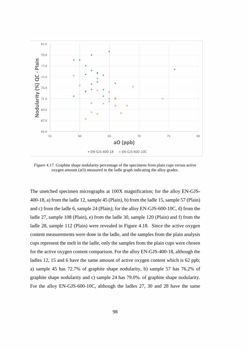
98

Figure 4.17. Graphite shape nodularity percentage of the specimens from plain cups versus active

oxygen amount (aO) measured in the ladle graph indicating the alloy grades.

The unetched specimen micrographs at 100X magnification; for the alloy EN-GJS-

400-18, a) from the ladle 12, sample 45 (Plain), b) from the ladle 15, sample 57 (Plain)

and c) from the ladle 6, sample 24 (Plain); for the alloy EN-GJS-600-10C, d) from the

ladle 27, sample 108 (Plain), e) from the ladle 30, sample 120 (Plain) and f) from the

ladle 28, sample 112 (Plain) were revealed in Figure 4.18. Since the active oxygen

content measurements were done in the ladle, and the samples from the plain analysis

cups represent the melt in the ladle, only the samples from the plain cups were chosen

for the active oxygen content comparison. For the alloy EN-GJS-400-18, although the

ladles 12, 15 and 6 have the same amount of active oxygen content which is 62 ppb;

a) sample 45 has 72.7% of graphite shape nodularity, b) sample 57 has 76.2% of

graphite shape nodularity and c) sample 24 has 79.0%. of graphite shape nodularity.

For the alloy EN-GJS-600-10C, although the ladles 27, 30 and 28 have the same

99

amount of active oxygen content which is 63 ppb; d) sample 108 has 68.2% of graphite

shape nodularity, e) sample 120 has 72.5% of graphite shape nodularity and f) sample

112 has 74.7%. of graphite shape nodularity. On the other hand, as it can be seen in

Figure 4.18, there is no significant difference in nodule shapes because the variation

in graphite shape nodularity is not as high as that it can be seen clearly.

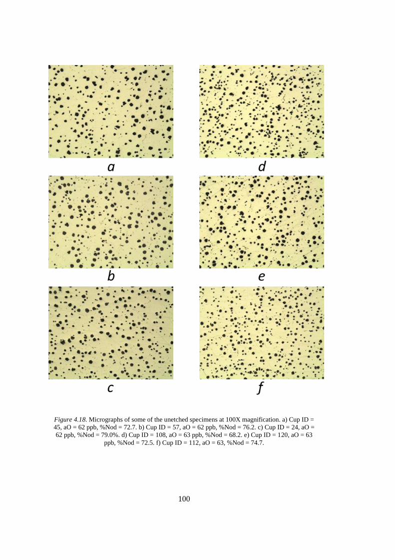
100

Figure 4.18. Micrographs of some of the unetched specimens at 100X magnification. a) Cup ID =

45, aO = 62 ppb, %Nod = 72.7. b) Cup ID = 57, aO = 62 ppb, %Nod = 76.2. c) Cup ID = 24, aO =

62 ppb, %Nod = 79.0%. d) Cup ID = 108, aO = 63 ppb, %Nod = 68.2. e) Cup ID = 120, aO = 63

ppb, %Nod = 72.5. f) Cup ID = 112, aO = 63, %Nod = 74.7.

101

CHAPTER 5

5. CONCLUSIONS

By this study on the cooling curve thermal analyses and oxygen activity analyses for

the estimation of microstructural properties of nodular cast iron, the following main

conclusions have been pointed out:

1. It was observed that the specimens of EN-GJS-600-10C grade have a higher

liquidus temperature level compared to EN-GJS-400-18 which is an expected effect

of the difference in their carbon equivalents. Average liquidus temperature difference

among two alloys was 15.0oC, and the average carbon equivalent difference among

two alloys was 0.17%.

2. It was observed that the specimens from plain analysis cups have lower upper

eutectic temperature (TEmax) values compared to the inoculant containing analysis

cups. Moreover, TEmax values of the specimens from inoculant containing cups are

mostly accumulated in a narrow range. For non-inoculated cups, TEmax is limited by

the low density of graphite particles. On the other hand, TEmax values of the

inoculated specimens are limited by the stable eutectic transformation temperature.

Therefore, TEmax values of inoculated EN-GJS-EN-400-18 specimens are aligned at

around 1152oC which is the stable eutectic transformation temperature. On the other

hand, the inoculated EN-GJS EN-GJS-600-10C specimens have TEmax values

aligned at around 1154oC. That 2oC of difference can be explained by the effect of

silicon content on the stable eutectic transformation temperature.

3. It was observed that the cooling curves of EN-GJS-600-10C specimens have

less time differences between the lower eutectic point and the end of freezing point

compared to EN-GJS-400-18 grade. These two points correspond to the start and the

end of graphite phase growth. Moreover, according to metallographic image analysis

102

results, the specimens of EN-GJS-600-10C grade have lower quantity of graphite

phase in their structure. Therefore, the lower total duration of eutectic transformation

arises from earlier termination of graphite phase growth.

4. It was observed that the specimens from the cups having 0.05% of inoculant

have liquidus temperatures in a similar level which is slightly higher compared to the

plain cups. In addition, the specimens from the cups having 0.10% and 0.15%

inoculant have liquidus temperatures in a level which is slightly lower compared to

the plain cups. Although pro-eutectic austenite nucleation does not require a high

quantity of excess energy, inoculant seems to help to the nucleation of pro-eutectic

austenite so that 0.05% of inoculant addition increases the liquidus temperature

slightly. Further addition of inoculant (0.10% and 0.15%) gave slight decrease in the

liquidus temperatures, and this can be explained by that the melt was saturated by the

nucleation sites, and further inoculation decreased the liquidus temperature by

increasing the carbon equivalent due to the silicon content of the inoculant.

5. It was observed that lower eutectic temperature (TEmin) values of the

specimens from plain cups are considerably lower compared to the inoculated cups.

Due to the presence of inclusion forming elements such as Ca, Al, Ce, Bi and Sb,

inoculant provides heterogeneous nucleation sites for the graphite phase so that

graphite nucleation requires a lower excess energy, thus less undercooling. In addition,

TEmin values of the specimens from the cups having Sb containing inoculant are

slightly lower compared to Bi containing inoculant. Therefore, inoculation effect of

Bi may be higher compared to Sb.

6. It was observed that the specimens of EN-GJS-600-10C grade have a lower

percentage of graphite phase compared to EN-GJS-400-18 which is a result of the

lower carbon content of EN-GJS-600-10C grade. Although silicon is a graphite former

and this grade has a high silicon content, if the carbon content is low, the amount of

graphite that can be formed is limited.

103

7. It was observed that graphite nodule count per unit area values of the

specimens from plain cups are considerably lower compared to the inoculated cups. It

is because heterogeneous nucleation sites provided by the inoculant yield in a higher

quantity of graphite nucleus formation which become graphite nodules as a result of

growth. In addition, the nodule counts of the specimens from the cups having Sb

containing inoculant are slightly lower compared to Bi containing inoculant.

Therefore, inoculation effect of Bi may be higher compared to Sb.

8. It was observed that graphite shape nodularity percentage values of the

specimens from plain cups are considerably higher compared to the inoculated cups.

The theory proposed by Zhou et al. claims a negative effect of Bi and Sb on the

graphite shape nodularity [26]. Since the inoculants that were used contain either Bi

or Sb, the negative effect claimed by the theory was observed on the structure of the

inoculated cup specimens.

9. It was observed that for both alloy grades, ferrite phase area percentage

increases when graphite nodule count per unit area increases. Higher number of

graphite nodules per unit area decreases the length of the diffusion path of carbon

atoms to reach to the graphite phase. Therefore, as the nodule count increases, carbon

content in the matrix decreases, and ferrite content increases. For the grade EN-GJS-

400-18, as a result of linear regression analysis, it was found that each 100 nodules

per mm2 yields in 7% increase in the ferrite content. For the grade EN-GJS-600-10C,

there could not be found a considerable regression since its specimens had almost no

pearlite.

10. It was observed that lower eutectic temperature (TEmin) versus graphite

nodule count per unit area graph follows a logistic function trend giving an S-shaped

(sigmoid) curve. As the nodule count goes from zero to infinity, TEmin follows; first

an exponential-like path, then an almost linear trend followed by a logarithmic-like

path.

The equation obtained from the data of EN-GJS-400-18 is given as;

104

𝑇𝐸𝑚𝑖𝑛 =27.39

1+𝑒𝑥𝑝[−0.012∗(𝑁𝑜𝑑𝑢𝑙𝑒𝐶𝑜𝑢𝑛𝑡−394.02)]+ 1120.44

where TEmin is in oC, and Nodule Count is in 1/mm2.

The equation obtained from the data of EN-GJS-600-10C is given as;

𝑇𝐸𝑚𝑖𝑛 =26.36

1+𝑒𝑥𝑝[−0.017∗(𝑁𝑜𝑑𝑢𝑙𝑒𝐶𝑜𝑢𝑛𝑡−416.96)]+ 1123.18

where TEmin is in oC, and Nodule Count is in 1/mm2.

These two correlations achieved by the regression analysis had satisfying r-square

values such that 0.94 for the data of EN-GJS-400-18 and 0.89 for the data of EN-GJS-

600-10C.

105

REFERENCES

1. G. Peter, D. B. Wagner, “Iron and Steel in Ancient China”, 1995, Bulletin de

l’Ecole française d’Extreme-Orient, Volume 82: pp. 426 - 428.

2. ASM International, “ASM Metals Handbook”, 2008, Volume 15: pp. 1445 -

1484.

3. T. Elbel, J. Senberger, A. Zadera, J. Hampl, “Behavior of Oxygen in Cast

Irons”, 2008, Archives of Materials Science and Engineering, Volume 33: pp. 111 -

116.

4. W. D. Callister, D. G. Rethwisch, “Fundamentals of Materials Science and

Engineering an Introduction”, 2010, 8th Edition: pp. 391 - 450.

5. DIN EN ISO 945-1:2009, “Graphitklassifizierung durch visuelle

Auswertung”, 2009, Mikrostruktur von Gusseisen.

6. Bundesverband der Deutschen Giesserei Industrie, “Gusseisen mit

Kugelgraphit: Herstellung - Eigenschaften – Anwendung”, 2007, Duesseldorf.

7. American Foundry Society, “Modern Casting”, 2012, 47th Census of World

Casting Production – Handbook: pp. 19.

8. J. Radzikowska, “Metallography and Microstructures of Cast Iron”, 2004,

ASM Metal Handbook, Volume 9: pp. 565 - 587.

9. V. Anjos, C. S. Ribeiro, J. Cunha, C. Gomes, “The Use of Thermal Analysis

to Compare Solidification Pattern and Evaluate Performance of Several Inoculants in

SG”, 2014, 71st World Foundry Congress, Spain.

10. DIN EN ISO 1563-3:2012, “Gusseisen mit Kugelgraphit”, 2012,

Giessereiwesen.

11. V. Anjos, “Use of Thermal Analysis to Control the Solidification Morphology

of Nodular Cast Irons and Reduce Feeding Needs”, 2015, University of Duisburg,

Germany.

12. R. D. Forrest, “What is the Optimum Base Iron Sulphur Content Prior to

Nodularization?”, 2006, Sorelmetal Technical Service - Rio Tinto Iron & Titanium

Inc.

13. G. M. Hansen, C. Hartung, D. White, “The Ductile Iron Treatment Process

Revisited”, 2014, 71st World Foundry Congress, Spain.

106

14. P. Cabanne, “Magnesium Cored Wire Treatment Advantages and

Disadvantages Vis-À-Vis Other Processes”, 2006, Sorelmetal Technical Service - Rio

Tinto Iron & Titanium Inc.

15. J. R. Brown, “Foundryman's Handbook”, 2000, Foseco Ferrous, UK.

16. W. Baumgart, J. Cunha, V. Anjos, “Het Enten van Gietijzer”, 2010, Gietwerk

Perspectief Magazine, Volume 5: pp. 5 - 12.

17. G. Lesoult, M. Castro, J. Lacaze, “Physical Modelling”, 1998, Solidification

of Spheroidal Graphite Cast Irons – Acta Metallurgica, Volume 46, Issue 3: pp. 983-

995.

18. W. Van der Perre: “Thermal Analysis of Cast Iron”, 2006, Heraeus Electro-

Nite International – Handbook.

19. W. F. Smith, “Structure and Properties of Engineering Alloys”, 1993, McGraw

Hill International: pp. 340.

20. J. Zhou, “Colour Metallography of Cast Iron”, 2009, China Foundry, Volume

6: pp. 57 - 65.

21. L. Svensson, A. Diószegi, K. Z. Liu, “Inoculation of Primary Austenite in Grey

Cast Iron”, 2006, Science and Processing of Cast Iron, Volume 8.

22. D. M. Stefanescu, “Science and Engineering of Casting Solidification”, 2009,

Springer Science + Business Media: pp. 1 - 4.

23. T. Skaland, F. Grong, T. Grong, “A Model for the Graphite Formation in

Ductile Cast Iron”, 1993, Metallurgical Transactions, Volume 24: pp. 2321 - 2347.

24. D. D. Double, A. Hellawell, “The Nucleation and Growth of Graphite”, 1994,

Modification of Cast Iron – Acta Metallurgica, Volume 43, Issue 6: pp. 2435 - 2442.

25. D. M. Stefanescu, “State of the Art in Solidification Modeling of Cast Iron”,

2006, Science and Processing of Cast Iron, Volume 8.

26. J. Zhou, S. Engler, W. Schmitz, “Formation of Austenite Shell around Nodular

Graphite and its Effect on Deterioration of Graphite”, 1990, AFS Transactions,

Volume 98: pp. 783 - 786.

27. W. Baumgart, “Untersuchung des Phasenübergangs von Flüssig nach fest am

Tertiären System Fe-C-Si unter Nichtgleichgewichtsbedingungen”, 2013, Lehrstuhl

für das Gesamte Giessereiwesen und Giesserei-Institut der RWTH Aachen, Germany.

28. C. R. Loper, R. W. Heine, M. D. Chaudhari, “Principles Involved in the Use

of Cooling Curves in Ductile Iron Process Control”, 1974, AFS Transactions, Volume

82: pp. 431 - 440.

107

29. V. Anjos, W. Baumgart, J. Cunha, “Grundlagen der Thermischen Analyse”,

2014, Seminar in OCC GmbH - Metallurgishe Regelkreise, Mönchengladbach.

30. D. M. Stefanescu, “The Physical Metallurgy of Cast Iron”, 1985: pp. 151.

31. W. Baumgart, V. Anjos, “Thermal Analysis of Ductile Iron”, 2009, Seminar

in OCC GmbH - Metallurgishe Regelkreise, Mönchengladbach.

32. I. G. Chen, D. M. Stefanescu, “Computer-Aided Differential Thermal Analysis

of Spheroidal and Compacted Graphite Cast Irons”, 1984, AFS Transactions, Volume

92: pp. 947 - 964.

33. D. M. Stefanescu, “Thermal Analysis – Theory and Application in

Metalcasting”, 2015 International Journal of Metalcasting, Volume 9: pp. 7 - 22.

34. R. Hummer, “Oxygen Activity of Ductile Iron Melts”, 1997, Advanced

Materials Research: pp. 269 - 276.

35. T. Elbel, J. Senberger, A. Zadera, R. Vladik, “State of the Art of Metal

Reoxidation Study of Iron Castings”, 2007, Archives of Materials Science and

Engineering, Volume 11: pp. 649 - 652.

36. J. Hampl, T. Valek, P. Lichy, T. Elbel, “Control of the Metallurgical

Processing of ICDP Cast Irons”, 2013, VSB Technical University of Ostrava, Czech

Republic.

37. F. Mampaey, D. Habets, F. Seutens, “The Use of Oxygen Activity

Measurement to Determine Optimal Properties of Ductile Iron during Production”,

2008, Foundry Research / Giessereiforschung, Volume 60, Issue 1: pp. 2 - 19.

38. Heraeus Electro-Nite International, "Oxygen Activity Measurement in Cast

Iron", 2015, Celox Foundry – Handbook: pp. 1 - 3.

39. F. Seutens, “Thermal Analysis of Cast Iron – Improvements in Measurement

Equipment”, 2017, Heraeus Electro-Nite International – Product and Application

Training, Belgium.

40. OCC GmbH, “Micr-O-Phase – Image Analyzer”, 2008, Handbook, Germany.

41. L. Rao, W. Tao, S. Wang, M. Geng, G. Cheng, “Influence of the Composition

Ratio of Manganese and Copper on the Mechanical Properties and the Machining

Performance of Ductile Iron”, 2014, Indian Journal of Materials Engineering &

Sciences, Volume 21: pp. 574 - 579.

42. OCC GmbH, “CSL – Regression Analysis Tool”, 2002, Handbook, Germany.

43. W. Stets, H. Löblich, G. Gassner, P. Schumacher, “Solution Strengthened

Ferritic Ductile Cast Irons – Properties, Production and Application”, 2014,

International Journal of Metalcasting, Volume 8, Issue 2: pp. 35 - 40.

108

44. Componenta Dokum A.Ş., “New Generation Ductile Irons”, 2014, 7th

International Ankiros Foundry congress.

cooling curve thermal analyses and oxygen activity - metu

Documents