hybrid meta-heuristic algorithms for the ... - metu
TRANSCRIPT
HYBRID META-HEURISTIC ALGORITHMS FOR THE RESOURCE
CONSTRAINED MULTI-PROJECT SCHEDULING PROBLEM
A THESIS SUBMITTED TO
THE GRADUATE SCHOOL OF NATURAL AND APPLIED SCIENCES
OF
MIDDLE EAST TECHNICAL UNVERSITY
BY
FURKAN UYSAL
IN PARTIAL FULLFILLMENT OF THE REQIREMENTS
FOR
THE DEGREE OF DOCTOR OF PHILOSOPHY
IN
CIVIL ENGINEERING
OCTOBER 2014

Approval of thesis:
HYBRID META-HEURISTIC ALGORITHMS FOR THE RESOURCE
CONSTRAINED MULTI-PROJECT SCHEDULING PROBLEM
submitted by FURKAN UYSAL in partial fulfillment of the requirements
for the degree of Doctor of Philosophy in Civil Engineering Department,
Middle East Technical University by,
Prof. Dr. Gülbin Dural
Dean, Graduate School of Natural and Applied Sciences
Prof. Dr. Ahmet Cevdet Yalçıner
Head of Department, Civil Engineering
Assoc. Prof. Dr. Rifat Sönmez
Supervisor, Civil Engineering Dept., METU
Examining Committee Members:
Assoc. Prof. Dr. Selçuk Kürşat İşleyen
Industrial Engineering Dept., Gazi University
Assoc. Prof. Dr. Rifat Sönmez
Civil Engineering Dept., METU
Prof. Dr. Talat Birgönül
Civil Engineering Dept., METU
Assist. Prof. Dr. Aslı Akçamete Güngör
Civil Engineering Dept., METU
Assist. Prof. Dr. Burak Çavdaroğlu
Industrial Engineering Dept. Işık University
Date:

iv
I hereby declare that all information in this document has been obtained and presented in accordance with academic rules and ethical conduct. I also declare that, as required by these rules and conduct, I have fully cited and referenced all material and results that are not original to this work.
Name, Last name:
Signature :
v
ABSTRACT
HYBRID META-HEURISTIC ALGORITHMS FOR THE RESOURCE
CONSTRAINED MULTI-PROJECT SCHEDULING PROBLEM
Uysal, Furkan
Ph. D., Department of Civil Engineering
Supervisor: Assoc. Prof. Dr. Rifat Sönmez
October 2014, 148 Pages
The general resource constrained multi-project scheduling problem (RCMPSP)
consists of simultaneous scheduling of two or more projects with common resource
constraints, while minimizing duration of the projects. Critical Path Method and
other scheduling methods do not consider resource conflicts and practically used
commercial project management software packages and heuristic methods provide
very limited solutions for the solution of the RCMPSP. Considering the practical
importance of multi-project scheduling and the fact that resource constraints impact
the schedules and costs significantly, achieving an adequate solution to the problem
is crucial for the construction sector.
In this research, we present a new hybrid algorithm which is based on genetic
algorithm, simulated annealing, backward forward improvement heuristics. The
performance of the algorithms is compared with the performances of the known
heuristic procedures and commonly used software packages using test instances
particularly developed for multi-project environment. Effectiveness of the
developed algorithm is further improved with the application of parallel computing
strategies with a Graphical Processing Unit (GPU). Results revealed that effective
resource management is a vital process but it is ignored by practitioners, heuristic
methods and current software packages. Proposed algorithm showed significant
improvements on the state of the art algorithms. It is also shown that parallel
computing strategies with a GPU has high potential for meta-heuristic applications

vi
specifically for construction management research area in which there is a
significant gap in the GPU research.
Key Words: Scheduling, Project Portfolio Management, Meta-heuristic algorithms,
GPU
vii
ÖZ
KAYNAK KISITLI BİRDEN FAZLA PROJENİN ÇİZELGELENMESİ
PROBLEMİ İÇİN ÜST-SEZGİSEL YÖNTEMLER
Uysal , Furkan
Doktora, İnşaat Mühendisliği Bölümü
Tez Yöneticisi: Doç. Dr. Rifat Sönmez
Ekim 2014, 148 Sayfa
Kaynak kısıtlı birden fazla projenin çizelgelenmesi problemi, iki ya da daha fazla
projenin ortak kaynak havuzu kullanılarak çizelgelenmesi ve toplam proje süresinin
kısaltılmasını amaçlamaktadır. Kritik yol yöntemi ve diğer çizelgeleme yöntemleri
kaynak kısıtlarını dikkate almamakta, pratikte kullanılan yazılımlar ve yazılımların
sezgisel yöntemleri ise probleme sınırlı çözümler sunabilmektedir. Birden fazla
projenin çizelgelenmesi probleminin inşaat sektöründe pratik önemi ve kaynak
kısıtlarının proje süresini ve maliyetini etkilediği düşünüldüğünde, probleme daha
iyi çözümler bulmanın gerekliliği ortaya çıkmaktadır.
Bu çalışmada, genetik algoritma, tavlama benzetimli algoritma ve ileri geri
iyileştirme sezgiseli kullanılarak yeni bir melez üst-sezgisel algoritma
geliştirilmiştir. Geliştirilen algoritma bu çalışma kapsamında oluşturulan ve birden
fazla projenin yer aldığı test projelerinde, pratikte kullanılan yazılımların sezgisel
yöntemleriyle ve bilinen diğer üst-sezgisel yöntemlerin sonuçlarıyla kıyaslanmıştır.
Algoritmanın etkinliğini artırmak için paralel hesaplama stratejisi geliştirilmiş ve
bir grafik işlem biriminde uygulaması yapılmıştır. Sonuçlar literatürdeki
algoritmalara kıyasla belirgin ilerlemeler kaydetmiş ve paralel hesaplama

viii
stratejilerinin grafik işlem birimiyle uygulamasının yapım yönetimi alanındaki
yüksek potansiyeli gösterilmiştir.
Anahtar Kelimeler: Çizelgeleme, Proje Portföy Yönetimi, Üst Sezgisel
Algoritmalar, Grafik İşlem Birimi

ix
DEDICATION
To my wife and expected twins...
x
ACKNOWLEDGEMENTS
“Sometimes life hits you in the head with a brick. Don't lose faith. I'm convinced
that the only thing that kept me going was that I loved what I did. You've got to find
what you love. And that is as true for your work as it is for your lovers. Your work
is going to fill a large part of your life, and the only way to be truly satisfied is to
do what you believe is great work. And the only way to do great work is to love
what you do. If you haven't found it yet, keep looking. Don't settle. As with all
matters of the heart, you'll know when you find it. And, like any great relationship,
it just gets better and better as the years roll on. So keep looking until you find it.
Don't settle” (A part from speech of Steve Jobs at Stanford University
commencement, 2005).
The question “Am I doing what I loved to do?” is a challenging question that I ask
myself many times. I worked at procurement and design departments of different
companies. I have been in public sector as a senior expert for many years. I also
enrolled in Ph.D. program at year 2007. I always kept looking. Sometimes I
demoralized, sometimes I was hopeful, sometimes both! Now, it has been 10 years
since my graduation! I finally realized that making research is what I want to do.
Endless thanks to those who help me to find “what I loved to do”.
First debt of gratitude must go to my advisor. I would like to thank Assoc. Prof. Dr.
Rifat Sönmez for his constant support and guidance. It was my pleasure to work
with him. It has been nine years since I met him and he is the most tolerant person
I have ever met. He constantly provided the vision and motivation that I need to
fulfill the Ph. D. program. From my master thesis up to now, we worked together
and contributed many academic endeavors. He has been not only an academic
advisor for me but also a friend whom I can phone whenever I got stuck.
I would like to thank Assoc. Prof. Dr. Selçuk Kürşat İşleyen for his valuable and
endless supports on mathematical modeling of the problem. He also provided critics
and directions on the subject of meta-heuristics. Industrial engineering view that he

xi
provided to me was very important. We also shared insightful discussions on my
thesis which I cannot forget.
I would like to thank to Prof. Dr. Talat Birgönül for his continuous supports from
the beginning of my academic life. It has been a great privilege for me to meet with
him.
I also want to thank Assist. Prof. Dr. Aslı Akçamete and Assist. Prof. Dr. Burak
Cavdaroğlu for taking part in my dissertation and for their further suggestions.
My family also provided valuable supports for this work. I would like to thank
specially to my wife Betül for her smiley face and motivations. She is my precious
at all time!
I have limitless thanks to my father Sadık Uysal, my mother Safiye Uysal and my
sister Hazal Uysal. Their love was my driving force.
This work is also supported by METU Scientific Research Projects (Project No:
BAP- 03-03-2010-04).
xii
TABLE OF CONTENTS
ABSTRACT ............................................................................................................ v
ÖZ ……………………………..………………………………………………..vii
ACKNOWLEDGEMENTS .................................................................................... x
TABLE OF CONTENTS ...................................................................................... xii
LIST OF TABLES ............................................................................................... xvi
LIST OF FIGURES ............................................................................................ xviii
LIST OF ABBREVIATIONS .............................................................................. xix
CHAPTERS
1. INTRODUCTION ............................................................................................ 1
1.1 Practical Importance of the Problem: ....................................................... 3
1.2 Prospects from the Thesis ......................................................................... 4
1.3 Scope and Limitations of the Thesis ......................................................... 5
1.4 Organization of the Thesis ........................................................................ 6
2. PROJECT SCHEDULING PROBLEMS AND LITERATURE REVIEW ..... 7
2.1. Definition of the Problem ...................................................................... 7
2.2. An Example Problem: How Can Activity Sequences Affect the
Duration of a Project? ...................................................................................... 8
2.3. Classification of RCPSP ..................................................................... 11
2.3.1. Elements of a RCPSP .................................................................. 13
2.3.1.1. Activities .................................................................................. 13
2.3.1.2. Resources ................................................................................. 13
2.3.1.3. Objective Function ................................................................... 14
2.3.1.4. Constraints ................................................................................ 14
2.3.1.5. Project Environment ................................................................. 14
2.4. Resource Constrained Single Project Scheduling Problem (RCPSP) . 16
2.4.1. Problem Definition ...................................................................... 16
2.4.2. RCPSP Literature ......................................................................... 18
xiii
2.4.2.1. Exact Methods ......................................................................... 19
2.4.2.2. Heuristics ................................................................................. 20
2.4.2.3. Meta-heuristics......................................................................... 24
2.5. Resource Constrained Multi-Project Scheduling Problem (RCMPSP)
……………………………………………………………………….31
2.5.1. Problem Definition ...................................................................... 31
2.5.2. RCMPSP Literature ..................................................................... 33
2.5.2.1. Exact Methods ......................................................................... 34
2.1.1.1. Heuristics ................................................................................. 35
2.1.1.2. Meta-heuristics......................................................................... 38
2.6. Parallel Computing Literature on Meta-heuristics.............................. 39
2.6.1. Introduction ................................................................................. 39
2.6.2. Literature Review of GPU Applications ..................................... 41
3. SOLUTION METHODS ............................................................................... 44
3.1. Test Instances ...................................................................................... 44
3.2. A Mathematical Formulation of RCPSP ............................................ 47
3.2.1. Parameters ................................................................................... 47
3.2.2. Variables ...................................................................................... 47
3.2.3. Constraints ................................................................................... 48
3.2.4. Objective Function ...................................................................... 49
3.2.5. Performance of Mathematical Model .......................................... 49
3.3. Heuristic Solutions .............................................................................. 51
3.3.1. MinSlack Rule ............................................................................. 51
3.3.2. SASP Rule ................................................................................... 52
3.3.3. MaxTWK Rule ............................................................................ 53
3.3.4. Backward Forward Heuristic ....................................................... 54
3.3.5. Performance Tests of Heuristics .................................................. 55
3.4. Meta-heuristic Solutions ..................................................................... 56
3.4.1. A Sole GA ................................................................................... 57
3.4.1.1. Chromosome Coding and Decoding ........................................ 57
3.4.1.2. Fitness Evaluation .................................................................... 58
3.4.1.3. Crossover ................................................................................. 59
xiv
3.4.1.4. Mutation ................................................................................... 59
3.4.1.5. Roulette Wheel Selection ......................................................... 60
3.4.1.6. Elitism ...................................................................................... 61
3.4.1.7. Parameter Setting ..................................................................... 61
3.4.1.8. Performance of the Algorithm.................................................. 61
3.4.2. A Sole SA .................................................................................... 64
3.4.2.1. Parameter Setting ..................................................................... 66
3.4.2.2. Performance of Algorithm ....................................................... 66
3.4.3. A hybrid GA-SA Algorithm ........................................................ 68
3.4.3.1. Performance of the Algorithm.................................................. 69
3.4.4. A Backward-forward Hybrid GA-SA Algorithm ........................ 71
3.4.4.1. Crossover, Mutation and Selection .......................................... 75
3.4.4.2. Integration of Simulated Annealing ......................................... 76
3.4.4.3. Performance of Algorithm ....................................................... 78
3.4.5. GPU Implementation of BFHGA ................................................ 85
3.4.5.1. Application of BFHGA on GPU .............................................. 85
3.4.5.2. Theory ...................................................................................... 85
3.4.5.3. Test of the Model ..................................................................... 87
4. ANALYSIS OF ALGORITHM PARAMETERS .......................................... 91
4.1. Two Level Factorial Design ................................................................... 91
4.1.1. Theory: ............................................................................................ 91
4.1.2. Application ...................................................................................... 94
4.1.2.1. Test of J30 Sets ........................................................................ 95
4.1.2.2. Test of J60 Sets ........................................................................ 97
4.1.2.3. Test of J120 Results ................................................................. 99
4.1.1. Interpretation from Main Effect Plots ........................................... 102
5. CONCLUSION ............................................................................................ 103
5.1. Summary and Discussion of Results ................................................. 103
5.2. Conclusion ......................................................................................... 106
REFERENCES .................................................................................................... 108
APPENDICES ..................................................................................................... 119

xv
A. Test Case Results ..................................................................................... 119
B. Code Details ............................................................................................. 121
C. Curriculum Vitae ..................................................................................... 147
xvi
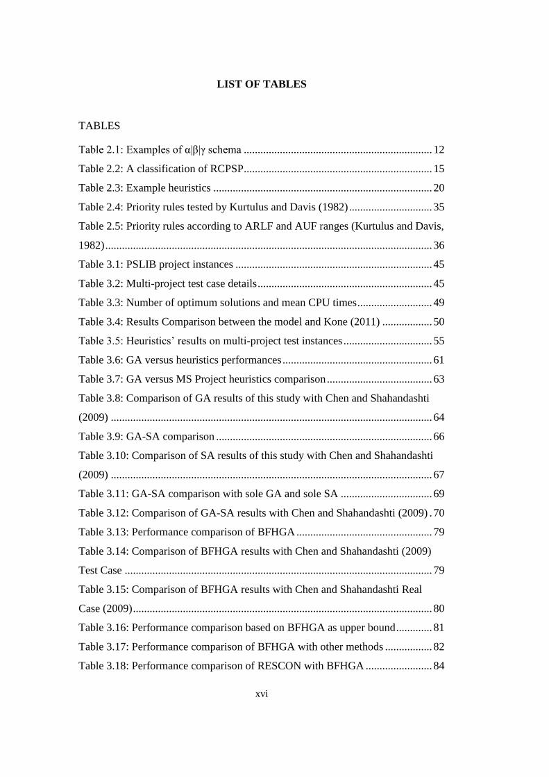
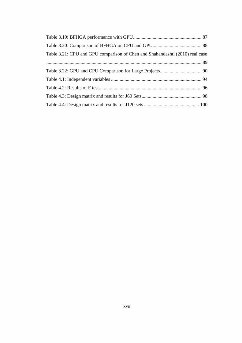
LIST OF TABLES
TABLES
Table 2.1: Examples of α|β|γ schema .................................................................... 12
Table 2.2: A classification of RCPSP .................................................................... 15
Table 2.3: Example heuristics ............................................................................... 20
Table 2.4: Priority rules tested by Kurtulus and Davis (1982) .............................. 35
Table 2.5: Priority rules according to ARLF and AUF ranges (Kurtulus and Davis,
1982) ...................................................................................................................... 36
Table 3.1: PSLIB project instances ....................................................................... 45
Table 3.2: Multi-project test case details ............................................................... 45
Table 3.3: Number of optimum solutions and mean CPU times ........................... 49
Table 3.4: Results Comparison between the model and Kone (2011) .................. 50
Table 3.5: Heuristics’ results on multi-project test instances ................................ 55
Table 3.6: GA versus heuristics performances ...................................................... 61
Table 3.7: GA versus MS Project heuristics comparison ...................................... 63
Table 3.8: Comparison of GA results of this study with Chen and Shahandashti
(2009) .................................................................................................................... 64
Table 3.9: GA-SA comparison .............................................................................. 66
Table 3.10: Comparison of SA results of this study with Chen and Shahandashti
(2009) .................................................................................................................... 67
Table 3.11: GA-SA comparison with sole GA and sole SA ................................. 69
Table 3.12: Comparison of GA-SA results with Chen and Shahandashti (2009) . 70
Table 3.13: Performance comparison of BFHGA ................................................. 79
Table 3.14: Comparison of BFHGA results with Chen and Shahandashti (2009)
Test Case ............................................................................................................... 79
Table 3.15: Comparison of BFHGA results with Chen and Shahandashti Real
Case (2009) ............................................................................................................ 80
Table 3.16: Performance comparison based on BFHGA as upper bound ............. 81
Table 3.17: Performance comparison of BFHGA with other methods ................. 82
Table 3.18: Performance comparison of RESCON with BFHGA ........................ 84
xvii
Table 3.19: BFHGA performance with GPU ........................................................ 87
Table 3.20: Comparison of BFHGA on CPU and GPU........................................ 88
Table 3.21: CPU and GPU comparison of Chen and Shahandashti (2010) real case
............................................................................................................................... 89
Table 3.22: GPU and CPU Comparison for Large Projects.................................. 90
Table 4.1: Independent variables .......................................................................... 94
Table 4.2: Results of F test .................................................................................... 96
Table 4.3: Design matrix and results for J60 Sets ................................................. 98
Table 4.4: Design matrix and results for J120 sets ............................................. 100
xviii
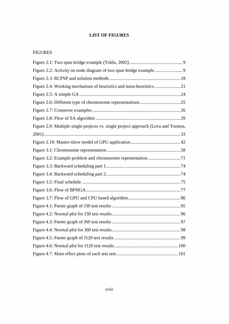
LIST OF FIGURES
FIGURES
Figure 2.1: Two span bridge example (Toklu, 2002) .............................................. 9
Figure 2.2: Activity on node diagram of two span bridge example ........................ 9
Figure 2.3: RCPSP and solution methods ............................................................. 18
Figure 2.4: Working mechanism of heuristics and meta-heuristics ...................... 21
Figure 2.5: A simple GA ....................................................................................... 24
Figure 2.6: Different type of chromosome representations ................................... 25
Figure 2.7: Crossover examples ............................................................................ 26
Figure 2.8: Flow of SA algorithm ......................................................................... 29
Figure 2.9: Multiple single projects vs. single project approach (Lova and Tormos,
2001) ...................................................................................................................... 33
Figure 2.10: Master-slave model of GPU application ........................................... 42
Figure 3.1: Chromosome representation ............................................................... 58
Figure 3.2: Example problem and chromosome representation ............................ 71
Figure 3.3: Backward scheduling part 1 ................................................................ 74
Figure 3.4: Backward scheduling part 2 ................................................................ 74
Figure 3.5: Final schedule ..................................................................................... 75
Figure 3.6: Flow of BFHGA.................................................................................. 77
Figure 3.7: Flow of GPU and CPU based algorithm ............................................. 86
Figure 4.1: Pareto graph of J30 test results ........................................................... 95
Figure 4.2: Normal plot for J30 test results ........................................................... 96
Figure 4.3: Pareto graph of J60 test results ........................................................... 97
Figure 4.4: Normal plot for J60 test results ........................................................... 98
Figure 4.5: Pareto graph of J120 test results ......................................................... 99
Figure 4.6: Normal plot for J120 test results ....................................................... 100
Figure 4.7: Main effect plots of each test sets ..................................................... 101

xix
LIST OF ABBREVIATIONS
ACO Ant Colony Optimization
CPM Critical Path Method
FCFS First Come First Served
GAs Genetic Algorithms
GPU Graphical Processing Unit
PERT Program Evaluation and Review
Technique
PSO Particle Swarm Optimization
PSP Project Scheduling Problem
RCMPSP Resource Constrained Multi-Project
Scheduling Problem
RCPSP Resource Constrained Project
Scheduling Problem
SA Simulated Annealing
SGS Schedule Generation Schema

This page is intentionally left blank.
1
CHAPTER 1
1. INTRODUCTION
Whether a project is as big as Marmaray Project which consists of 76 km long
railway, various type of tunnels, three underground stations, 37 surface stations,
165 bridges, 63 culverts, many yards, workshops, maintenance facilities, and
procurement of 440 modern rolling stocks (Lykke and Belkaya, 2005) or as small
as a single floor construction of a building, planning and scheduling is indispensable
in order to control total project execution time and its overall cost. Even on a single
floor construction of a building, the sequence of the activities, dependencies
between activities and resource allocation can be complicated. Without planning
and scheduling, project will end with a chaos; jobs execute in a randomly manner
and it would not be possible finish the project within planned time and cost. This
results in a significant loss for a company.
This issue has been the focus of extensive research in project management since
1900s. Researchers tried to define ways to plan and schedule projects by dividing
them into manageable parts, drawing charts and developing algorithms. Since then,
Gantt charts and the well-known critical path method (CPM) has been extensively
used and taken for granted as good scheduling tools for small to large scale projects
especially in the construction industry.
The first attempt to divide a project into manageable parts was proposed with Gantt
charts at 1900s during World War I (Meredith and Mantel, p.354, 1995). In this
method, activities are shown according to their start and finish times on a horizontal
table called bar charts. Taken for granted as an easy way of representing project
plan, Gantt chart is used commonly in the construction sector. Main weakness of
Gantt chart is its complexity in making large scale projects due to lack of
precedence relations among activities harder to manage.
2
After 1950s, CPM has been one of the most commonly used method to model and
control a project within its own assumptions and boundaries. In this method, critical
paths are defined as those work orders in which if an activity is delayed whole
project is delayed at the same time. Project is divided into manageable parts; work
packages and activities. Activity relations are shown with arcs. Due to its visual
aspect, a project can be portrayed as a network and it is possible to see predecessor
and successor relations between activities. A logical framework is schematized
through the activities and minimum time algorithm can be applied to the problem.
PERT technique which followed CPM, was incorporated to deal with stochastic
nature of projects. Since real life complexity brings uncertainty to activity duration
estimates, PERT brought the ability to incorporate with this uncertainties. Using
PERT, one can find either the probability of completing a project to a given date or
find time duration corresponding to a probability value (Cottrell, 1999).
However, with Gantt charts, CPM and PERT decision makers are focused on time
aspects of a project without considering the resource limitations. This ‘time only”
analysis, brings a main drawback since resource limitations are not considered.
Therefore, its practicability decreases significantly. In practice, resource conflicts
arise when two or more activities are demanding same scarce resources. Due to the
scarcity of resources, a trade-off exits between available resources and activity
durations. From a company level perspective, situation is magnified if there is more
than one project. Neither Gantt chart nor CPM or PERT methods are capable of
dealing with resource management. Therefore, a complete tool of scheduling should
not only consider “time only” analysis of projects but also should reflect resource
limitations. Since the late 1980s there has been a growing interest on scheduling
algorithms that considers resource limitations.
In scheduling where real life complexity drives us to use some models (Gantt
Charts, CPM and PERT) and models bring drawbacks (resource management),
resource constrained project scheduling problem (RCPSP) arises. The objective of
the problem is to determine a start date for each activity in such a way that
precedence and resource constraints are satisfied, and at the same time project
3
duration is minimized. If this problem is in a corporate level where more than one
project is managed, it is called as resource constrained multi-project problem
(RCMPSP).
During the last decades RCPSP has become a well-known standard problem in
project scheduling (Hartmann and Briskorn, 2010), and has attracted numerous
researchers from multiple areas including operation research, and construction
management.
While majority of projects are scheduled on a multi-project environment, most
research on RCPSP have focused on single projects (Kurtulus and Davis, 1982;
Krüger and Scholl, 2009; Browning and Yassine, 2010). Despite the importance of
RCMPSP in practice, there are few studies on this problem. Therefore, there is a
significant potential for improving the state–of–the–art algorithms. Hence, the main
objective of this study is to develop a new efficient optimization algorithm for the
RCMPSP to fill the gap within the literature.
1.1 Practical Importance of the Problem:
In construction management practice since the size of projects are comparably
bigger than any other sector, possible delays, crew size and equipment selection,
and resource allocation process could lead to significant problems like cost overruns
or longer project durations. Project delays and delay costs affect negatively on the
profit and repetition of the company. Due to the characteristics of construction work
such as unforeseen events, risks involved, multi-dimensional partners, cultural
differences, resource demands and resources assigned to a project is rarely met. In
addition, shorter project life cycles due to time pressure, little tolerance to cost
overruns due to the market competition and high resource costs makes sector more
vulnerable to bad scheduling practices. This makes scheduling process of
construction projects more complex than any other sector. Therefore, both the effect
of costs, prestige and sustainability of company, finding effective, efficient and
good enough solutions to project scheduling problem (PSP) is very important.
4
It is generally known that today's business environment is challenging and
companies manage multiple projects which share enterprise resources (Payne,
1995; Lova and Tormos, 2001; Liberatore and Pollack-Johnson, 2003). Sharing the
resources requires corporate level optimization of available resources. Frequently
the availability of the enterprise resources is limited, and is not sufficient to
concurrently schedule the activities. In these circumstances, optimal allocation of
limited enterprise resources is crucial for minimizing the project durations and costs
to achieve project portfolio success.
Improving the solution algorithms’ performances would improve the state of the art
algorithms and current software packages. Eventually, an efficient algorithm that
will solve the real life problems within a reasonable time period would results in
better organized schedules, better resource allocation and cost reductions for
corporate level. Therefore, the need for better algorithms is a practical need and
serves a great opportunity to develop commercial software packages.
1.2 Prospects from the Thesis
Since RCPSP is an NP-hard1 problem (Blazewicz et al., 1983), RCMPSP is also
NP-hard. The complexity2 of the problem sets a boundary to the solution methods
of the problem. Therefore, it can be solved by exact methods only for small projects.
Within the RCMPSP, researches are oriented to priority based heuristics and meta-
heuristics which do not guarantee the optimal solution. Performances of the
algorithms are arguable and as the network complexity3 increases performance of
the algorithm reduces significantly (Kolish, 1999). Moreover, extensively used
popular software packages’ performances on resource allocation are arguably low
and need to be improved.
1 NP-Hard: A problem is called non-deterministic (NP) polynomial if its solution cannot be evaluated in polynomial time and
solution is not guaranteed. No known exact algorithms can be able to solve the problem for large instances and only approximate solutions or heuristics are available (Yang, p.9, 2008).
2 Complexity: A measure of the efficiency of the algorithm. For details see ( Yang, p.24, 2008) 3 Network Complexity (NC) is average number of precedence relations per activity (Kolish, 1999).
5
The main objective of this research is to develop an efficient algorithm for obtaining
optimum or near-optimum solutions to the RCMPSP. Meta-heuristics are used to
improve the current state of the art algorithms.
As an output, a sole genetic algorithm (GA), a sole simulated annealing (SA)
algorithm, a backward-forward implemented GA and finally, a hybrid backward-
forward GA-SA algorithm is developed. Developed algorithms are tested with
known test instances. Optimum solutions are also used for comparisons. Previous
results from the literature are also used in order to compare algorithm performances.
An educational software RESCON (Deblaere et al., 2011), and its tabu search
algorithm is used for base line solutions.
Computer programs are written with Microsoft Visual Studio 2010 and coded with
C and C++ programing languages. In order to test the parallel programing effects
on meta-heuristics, final algorithm is implemented with a parallel evolutionary
strategy and computed on a Graphical Processing Unit (GPU).
1.3 Scope and Limitations of the Thesis
RCPSP is stemmed from job-shop scheduling problem in operational research. Job-
shop scheduling problem has various cases so does RCPSP and RCMPSP. Basic
problem definition is used throughout the study and mathematical model of the
problem will be given in the following sections. In the scope of this research,
activity pre-emption is not allowed4. Every activity is assumed to have non-
negative durations and resource usage. All parameters are assumed to be
deterministic and portfolio has a static structure. Activity durations are assumed to
be discrete. Finish to Start (FS) activity relation is used for majority of the test
cases but model can handle other relations, too. As network complexities of each
test instance increases, computational time increase significantly. Therefore, most
of the tests were solved with time limits.
4 It is stated that duration of an activity cannot be split up.

6
1.4 Organization of the Thesis
Following chapters are organized as follows: In the second chapter project
scheduling problems are summarized and literature survey of RCPSP and RCMPSP
are given. In the third chapter, a mathematical model of the problem is illustrated.
Problem is solved also heuristics and meta-heuristics. It includes novel meta-
heuristic solution that is developed in the scope of this thesis. Details of the
algorithms and their test results are given. Fourth chapter is for experiment design
of algorithm parameters. Finally, a conclusion section is given as the last chapter.
7
CHAPTER 2
2. PROJECT SCHEDULING PROBLEMS AND LITERATURE REVIEW
2.1.Definition of the Problem
Project scheduling problems (PSP) are one of the important practical optimization
problems which are extensively studied in operations research, management
science and construction management research area. Due to the practical
importance, some methods already been incorporated and many software packages
has been developed. PSP in general consists of three different problems. These are
time-cost tradeoff analysis, resource leveling problem and resource allocation
problem. In time-cost tradeoff analysis the tradeoff between duration of an activity
and cost of that activity is examined. It is known that in order to meet deadline
requirements of a schedule if more resource is added to the project, direct cost of
an activity increases. Adding more resource decreases the activity duration. This
tradeoff should be carefully examined in order to determine the extra cost of adding
new resources. Thus, in this type of problems, normal cost and crash cost of the
project is analyzed and decision is made based on time-cost tradeoff analysis. Time-
cost tradeoff analysis may include single objectives such as minimization of the
cost or minimization of duration (Ke and Liu, 2005) or multi objective cases such
as the work of Zheng et al., (2004). Different from time cost tradeoff problem, in
resource leveling problem aim is to obtain smooth resource curve so as to minimize
resource fluctuations under fixed project duration. It is assumed to have enough
resources for the project and fluctuations in resource demand is minimized. These
fluctuations mean idle resources and extra cost to the project. Leveling is done with
shifting non critical activities within their available floats (Easa, 1989). As for
resource allocation problems, resources are assigned to activities so as to optimize
certain objectives. In this type of problems, mostly single objectives such as cost
minimization is used and in recent studies multi objective resource allocation
problem can also be found in the literature (Osman et al., 2005; Chaharsooghi and
8
Kermani, 2008). Being a special case of resource allocation problems, RCPSP can
be extensively found in the literature. RCPSP can be defined as finding an optimal
solution for the sequence of activities based on a predefined objective function
where resources are limited. RCPSP and its multi-project case are the objectives of
this research and will be examined in the following chapters in detail. Although
PSP problems are complicated problems, a minimum time algorithm is extensively
used in the literature for solution purposes. This method is called CPM.
Practically used and taken for granted as a good scheduling method, CPM can be
considered as a basic solution methodology for the scheduling problem, but
explicitly it is assumed that there is no resource constraints. Most project scheduling
software packages are capable of serving as good CPM scheduler and get visual
help to practitioners. CPM and software combinations are extensively used in the
practice. Nevertheless, the unlimited resource assumption makes this method more
vulnerable to bad scheduling practices.
In practice, there are usually limitations for a number of resources. Thus, under the
consideration of resource limitation basic PSP becomes a mathematical problem
which is more complicated than the simple model and cannot be solved with CPM
model.
2.2. An Example Problem: How Can Activity Sequences Affect the Duration
of a Project?
A scheduler has to decide activity sequences of a project under given resource
limitations. Deciding the right activity sequence is a key choice since some activity
sequences may result longer durations, some results shorter durations under same
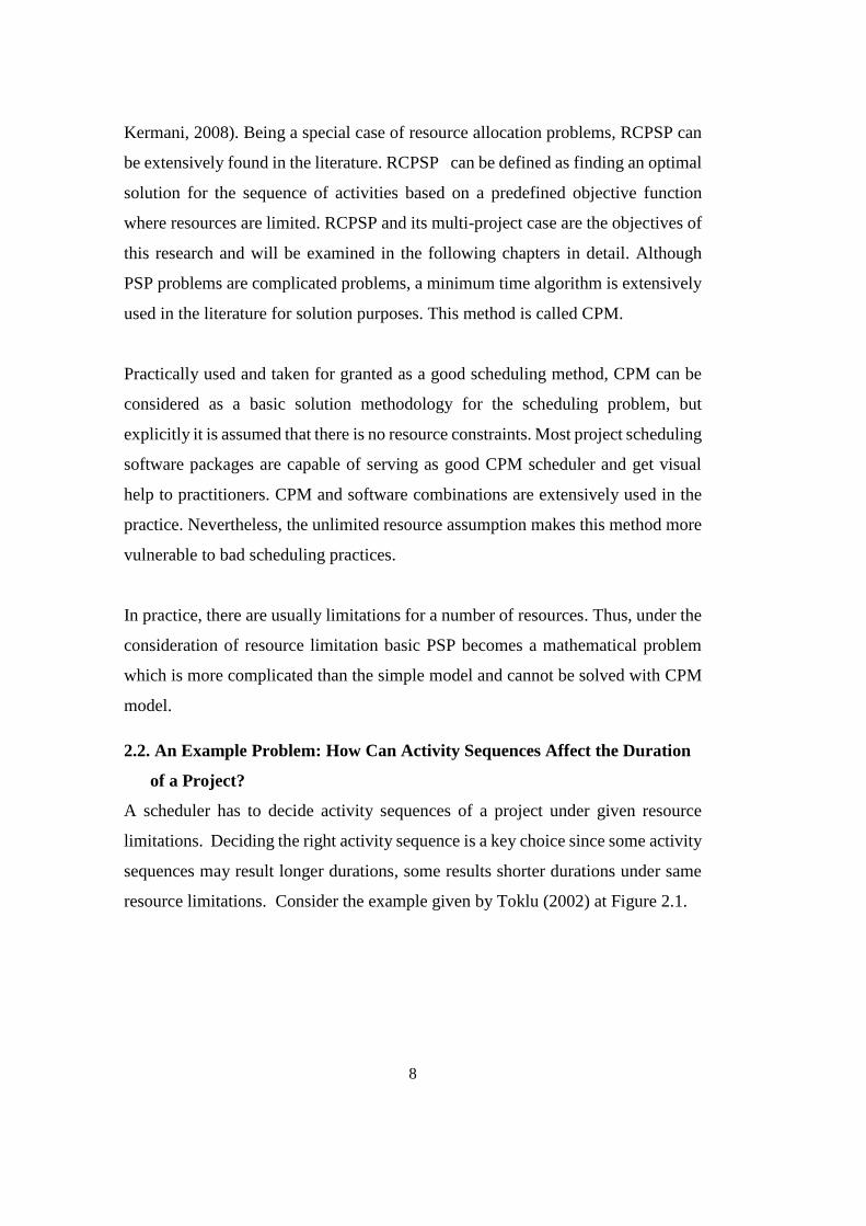
resource limitations. Consider the example given by Toklu (2002) at Figure 2.1.
9
Figure 2.1: Two span bridge example (Toklu, 2002)
A two span bridge construction is given as an example of the importance of activity
sequences. Suppose there exists only one excavation team, one pier construction
team and one span construction team. Considering the method of construction one
can say that construction may be started with any of the pier excavation: A1, B1,
and C1. Construction either follows the same locations in order to start pier works
as soon as possible or follows other locations independent from excavation works.
For example, if excavation is selected as A1, B1 and C1, pier construction would
follow A2, B2, C2 sequences in order to start pier construction as soon as possible.
A different strategy can also be selected such as starting pier construction after all
of the excavation work is finished. That way would obviously results longer
duration than expected. Assuming the strategy that pier construction work follows
excavation work in advance, possible construction sequences are as follows.
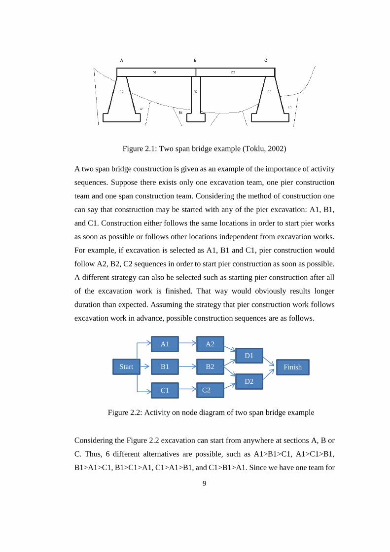
Considering the Figure 2.2 excavation can start from anywhere at sections A, B or
C. Thus, 6 different alternatives are possible, such as A1>B1>C1, A1>C1>B1,
B1>A1>C1, B1>C1>A1, C1>A1>B1, and C1>B1>A1. Since we have one team for
Start
A1
B1
C1
A2
B2
C2
D1
D2
Finish
Figure 2.2: Activity on node diagram of two span bridge example
10
pier construction and we have a strategy that pier construction follows excavation
work in advance, possible pier construction alternatives are A2>B2>C2,
A2>C2>B2, B2>A2>C2, B2>C2>A2, C2>A2>B2, and C2>B2>A2. And also 2
different deck constructions are possible, such as D1>D2 or D2>D1. It makes
totally 6x2 different construction sequences. If we consider the pier construction
team is not dependent on excavation team, we would have 6 x 6 x 2 different
combinations.
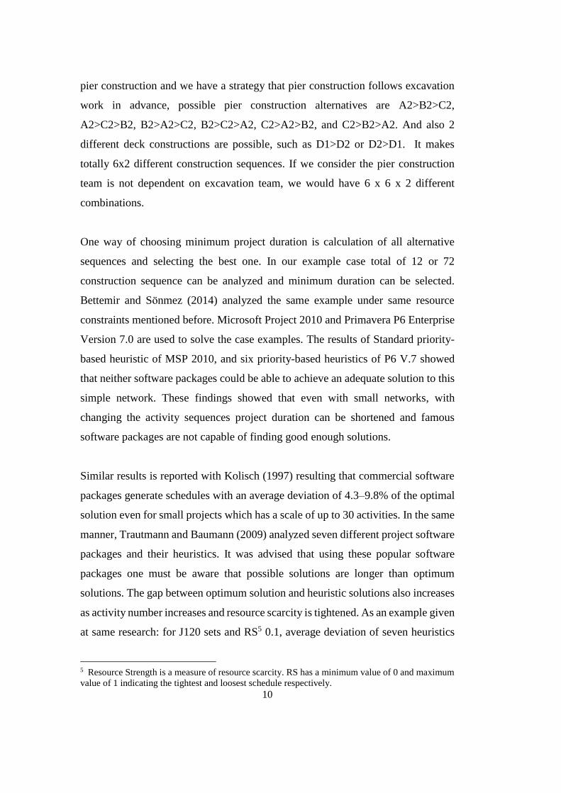
One way of choosing minimum project duration is calculation of all alternative
sequences and selecting the best one. In our example case total of 12 or 72
construction sequence can be analyzed and minimum duration can be selected.
Bettemir and Sönmez (2014) analyzed the same example under same resource
constraints mentioned before. Microsoft Project 2010 and Primavera P6 Enterprise
Version 7.0 are used to solve the case examples. The results of Standard priority-
based heuristic of MSP 2010, and six priority-based heuristics of P6 V.7 showed
that neither software packages could be able to achieve an adequate solution to this
simple network. These findings showed that even with small networks, with
changing the activity sequences project duration can be shortened and famous
software packages are not capable of finding good enough solutions.
Similar results is reported with Kolisch (1997) resulting that commercial software
packages generate schedules with an average deviation of 4.3–9.8% of the optimal
solution even for small projects which has a scale of up to 30 activities. In the same
manner, Trautmann and Baumann (2009) analyzed seven different project software
packages and their heuristics. It was advised that using these popular software
packages one must be aware that possible solutions are longer than optimum
solutions. The gap between optimum solution and heuristic solutions also increases
as activity number increases and resource scarcity is tightened. As an example given
at same research: for J120 sets and RS5 0.1, average deviation of seven heuristics
5 Resource Strength is a measure of resource scarcity. RS has a minimum value of 0 and maximum
value of 1 indicating the tightest and loosest schedule respectively.
11
were about %24 where the minimum value is %17. 93 and maximum value is %39.
53.
Although it is possible to find minimum duration under all possible activity
sequences, it can only be possible for such small networks. As the network size and
resource combinations increase, it becomes impossible to analyze every sequence
combination of a schedule. As network size and resource number increases, the
combination of resource/activity increases exponentially. This phenomena is
known as the “combinatorial explosion” which imply that since the problem itself
is NP-Hard (Blazewicz et al., 1983), no polynomial time algorithm is capable of
solving the problem. Therefore, this huge amount of data cannot be calculated by
hand.
Although some exact methods do exist which guarantee the optimum solution, their
capabilities are limited (Chen et al., 2010). Due to its limited applicability to large
problem instances, some heuristics and meta-heuristics are extensively used.
2.3.Classification of RCPSP
RCPSP has been a standard problem in operations research and since 1960s
abundant amount of research has been reported. This section is devoted to its
classification efforts.
With the efforts given to the problem itself and the variations of the problem in the
literature, classification need was emerged. In 1997 a workshop was conducted at
the University of California, Riverside and a classification schema was established
(Demeulemeester and Herroelen, p: 72, 2002). Brucker et al., (1999) classified the
RCPSP along with a notation procedure. This notation is stemmed from machine
scheduling and follows α|β|γ schema which represents resource characteristics,
activities and objective functions. Further attempts accepted the works of Brucker
et al., (1999) and Herroelen et al., (1999) which are basically built upon machine
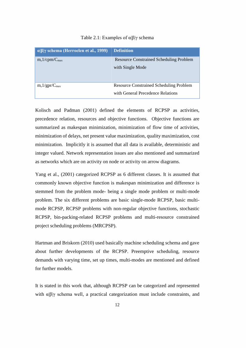
scheduling literature. Example of Herroelen et al., (1999) can be seen at Table 2.1.
12
Table 2.1: Examples of α|β|γ schema
α|β|γ schema (Herroelen et al., 1999) Definition
m,1/cpm/Cmax Resource Constrained Scheduling Problem
with Single Mode
m,1/gpr/Cmax Resource Constrained Scheduling Problem
with General Precedence Relations
Kolisch and Padman (2001) defined the elements of RCPSP as activities,
precedence relation, resources and objective functions. Objective functions are
summarized as makespan minimization, minimization of flow time of activities,
minimization of delays, net present value maximization, quality maximization, cost
minimization. Implicitly it is assumed that all data is available, deterministic and
integer valued. Network representation issues are also mentioned and summarized
as networks which are on activity on node or activity on arrow diagrams.
Yang et al., (2001) categorized RCPSP as 6 different classes. It is assumed that
commonly known objective function is makespan minimization and difference is
stemmed from the problem mode- being a single mode problem or multi-mode
problem. The six different problems are basic single-mode RCPSP, basic multi-
mode RCPSP, RCPSP problems with non-regular objective functions, stochastic
RCPSP, bin-packing-related RCPSP problems and multi-resource constrained
project scheduling problems (MRCPSP).
Hartman and Briskorn (2010) used basically machine scheduling schema and gave
about further developments of the RCPSP. Preemptive scheduling, resource
demands with varying time, set up times, multi-modes are mentioned and defined
for further models.
It is stated in this work that, although RCPSP can be categorized and represented
with α|β|γ schema well, a practical categorization must include constraints, and
13
project environment in addition to the schema. More specifically, model based
constraints can be added and the problem becomes more specific for important
practical cases. Problems can be modeled in a static environment where all jobs are
available before the scheduling starts or problems may be in a dynamic environment
where any job may enter to the scheduling process while scheduling is going on.
Within all literature so far it can be stated that, at least 5 main factors affect the
problem itself. These are; activities, resources, objective functions, constraints and
project environment. In order to define each factor and be more specific each factor
is defined in the following section.
2.3.1. Elements of a RCPSP
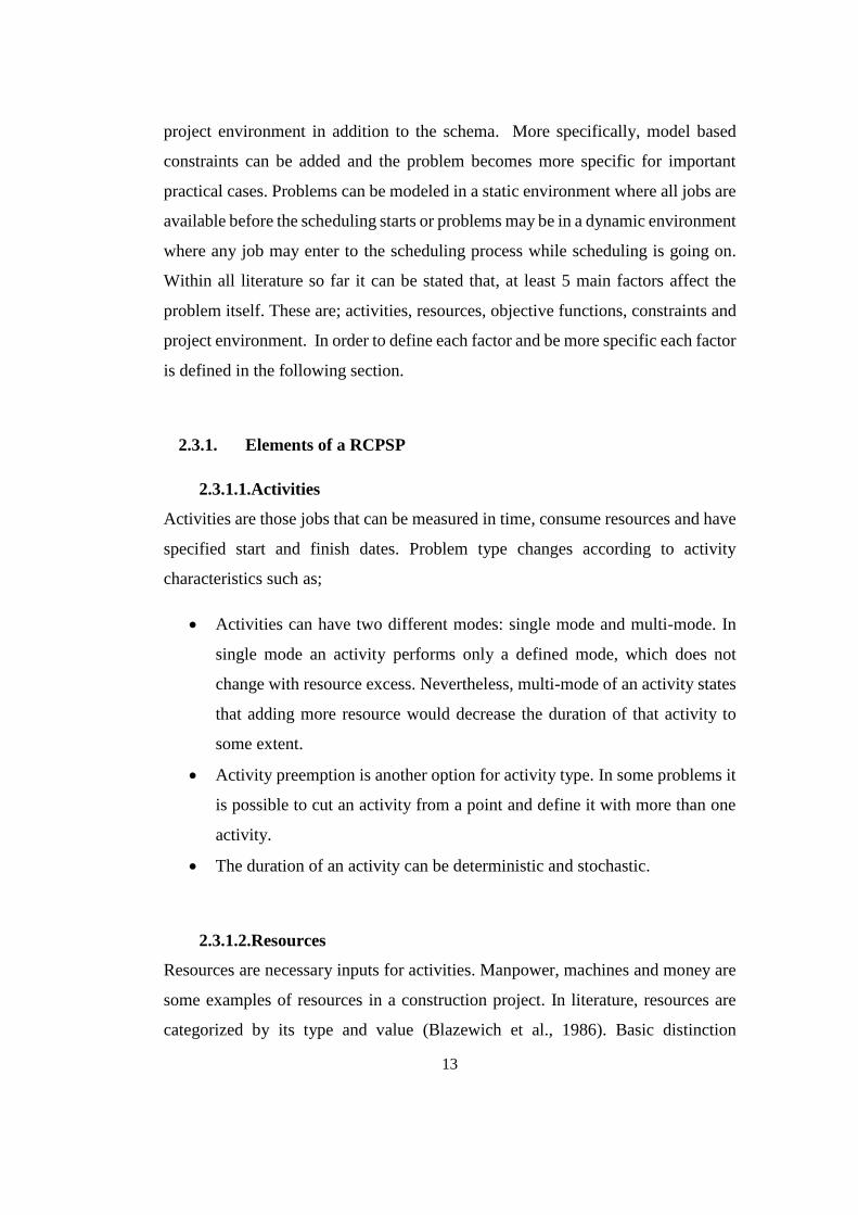
2.3.1.1.Activities
Activities are those jobs that can be measured in time, consume resources and have
specified start and finish dates. Problem type changes according to activity
characteristics such as;
Activities can have two different modes: single mode and multi-mode. In
single mode an activity performs only a defined mode, which does not
change with resource excess. Nevertheless, multi-mode of an activity states
that adding more resource would decrease the duration of that activity to
some extent.
Activity preemption is another option for activity type. In some problems it
is possible to cut an activity from a point and define it with more than one
activity.
The duration of an activity can be deterministic and stochastic.
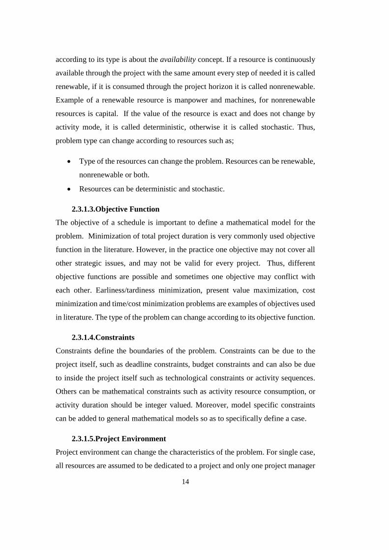
2.3.1.2.Resources
Resources are necessary inputs for activities. Manpower, machines and money are
some examples of resources in a construction project. In literature, resources are
categorized by its type and value (Blazewich et al., 1986). Basic distinction
14
according to its type is about the availability concept. If a resource is continuously
available through the project with the same amount every step of needed it is called
renewable, if it is consumed through the project horizon it is called nonrenewable.
Example of a renewable resource is manpower and machines, for nonrenewable
resources is capital. If the value of the resource is exact and does not change by
activity mode, it is called deterministic, otherwise it is called stochastic. Thus,
problem type can change according to resources such as;
Type of the resources can change the problem. Resources can be renewable,
nonrenewable or both.
Resources can be deterministic and stochastic.
2.3.1.3.Objective Function
The objective of a schedule is important to define a mathematical model for the
problem. Minimization of total project duration is very commonly used objective
function in the literature. However, in the practice one objective may not cover all
other strategic issues, and may not be valid for every project. Thus, different
objective functions are possible and sometimes one objective may conflict with
each other. Earliness/tardiness minimization, present value maximization, cost
minimization and time/cost minimization problems are examples of objectives used
in literature. The type of the problem can change according to its objective function.
2.3.1.4.Constraints
Constraints define the boundaries of the problem. Constraints can be due to the
project itself, such as deadline constraints, budget constraints and can also be due
to inside the project itself such as technological constraints or activity sequences.
Others can be mathematical constraints such as activity resource consumption, or
activity duration should be integer valued. Moreover, model specific constraints
can be added to general mathematical models so as to specifically define a case.
2.3.1.5.Project Environment
Project environment can change the characteristics of the problem. For single case,
all resources are assumed to be dedicated to a project and only one project manager
15
is assumed to be in charge of resource allocation. Nevertheless, in a multi project
environment, resources are considered as corporate resources. Therefore, resource
allocation in a top level managers’ perspective makes this problem more complex
than the single case.
Also, multi project environment characteristics may be different. Being a static
environment, all jobs are known and during scheduling no new job is added. In this
form of problems once a mathematical model is determined, it would not change
until the schedule has been completed. On the other hand, dynamic environment
can change mathematical model significantly. Therefore, project environment
should be considered in classifications. The importance of the project environment
becomes significant when some heuristics are applied to the problem. For example,
if slacks are determined considering dynamic environment, it should be updated
within a routine while in a static case slacks will not change until scheduling is over.
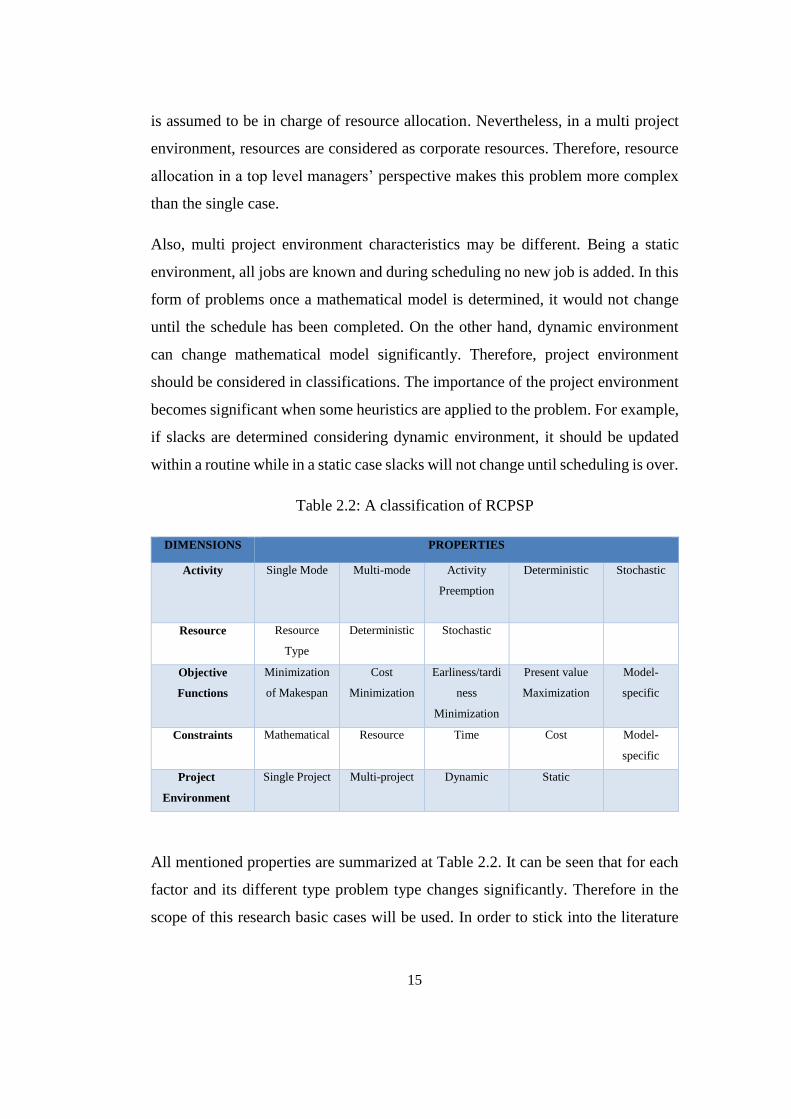
Table 2.2: A classification of RCPSP
DIMENSIONS PROPERTIES
Activity Single Mode Multi-mode Activity
Preemption
Deterministic Stochastic
Resource Resource
Type
Deterministic Stochastic
Objective
Functions
Minimization
of Makespan
Cost
Minimization
Earliness/tardi
ness
Minimization
Present value
Maximization
Model-
specific
Constraints Mathematical Resource Time Cost Model-
specific
Project
Environment
Single Project Multi-project Dynamic Static
All mentioned properties are summarized at Table 2.2. It can be seen that for each
factor and its different type problem type changes significantly. Therefore in the
scope of this research basic cases will be used. In order to stick into the literature
16
and to be on the side of known problem types, basic RCPSP problems is given in
the following paragraphs.
Case Example #1 “Basic Deterministic Case”: In this case, all parameters are
assumed to be deterministic and resources are assumed to be unlimited. This very
broad definition of PSP is generally used by practitioners and a minimum time
algorithm is used to solve the problem. This minimum time algorithm is called
CPM. In this method, aim is to find a schedule which is consisting of critical paths
orders. The time frame of a schedule is captured and effect of an activity delay can
be determined from the network. Resources are assumed to be unlimited but as a
final schedule resource leveling strategy is used in order to minimize resource
fluctuations.
Case example #2 “Deterministic Case with Resource Constraints”: In addition to
basic deterministic case, the resource limitation constraint is added and the problem
and it is called RCPSP. If more than one project is under consideration problem
becomes RCMPSP. Both analytical and heuristic solution attempts are available in
the literature and the model will be studied in the next sections.
Case example #3 “Multi-mode with Resource Constraints”: In this case, either
activity durations or resource limitation can vary. For multi-mode PSP, a set of
different modes is available for execution. For example, in a mode 1 worker can
work 6 days and finish the job, while if 2 workers work in the same amount of work
they can finish the job in 3 days. This type of variable crew assignment is possible.
Different from the mode of the activity, activity duration can be a random variable
which obeys a probability distribution.
From this point further, case example #2 will be analyzed in detail:
2.4.Resource Constrained Single Project Scheduling Problem (RCPSP)
2.4.1. Problem Definition
With the basic assumptions of CPM, a time order of activities can be modeled and
schedule of a project can be drawn as nodes and arrows. The unlimited resource
17
assumption is valid in this method and this assumption is not suited in majority of
the real life problems. More importantly, if resources are not meeting with the
demands of the activities, activities should be shifted to a time where resources are
adequate. Therefore, real durations under the resource limitations would be beyond
the CPM duration. Then, a question arises “how can this duration shift be
minimized?” and the problem of RCPSP arises.
RCPSP modeled in this research is aiming to find an optimal scheduling of a set of
activities within a network while precedence and resource constraints are not
violated. The precedence constraints force an activity to be started within an
imposed time frame after all of its predecessors are completed. It is a reality that
activity execution requires an amount of resource usage and some of the resources
are limited. Thus, resource constraints force an activity to consume a limited
amount of resources. Within the constraints of activities and resource limitations,
more than one schedules can be generated which would have different project
durations-some are longer while some are shorter. Therefore, the aim in RCPSP is
to find the minimum duration of a project without violating the assumptions of the
problem.
The basic RCPSP is modeled in a project network G (N, A) with a set of N nodes
and A arcs, each node representing the project activities using the activity on node
representation. Each activity j has a duration of dj, finish time Fj and resource usage
ri. The activities in the network are subject to precedence constraints which force
to start an activity only after completing its predecessor(s). It is assumed that there
are m renewable resource types, with a per period availability Rm.
The problem is mathematically modeled in this way;
The objective is to:
Minimize Total Project Duration
∑ 𝐹𝑛𝑖 .................................................................................................. (2.1)
Where some constraints exist such that:
18
𝐹𝑖 < 𝐹𝑗 − 𝑑𝑗…………………………………………………..…………….(2.2)
𝑟𝑗 < 𝑅𝑚......................................................................................................... (2.3)
𝐹𝑗 , 𝑟𝑗 , 𝑑𝑗 ≥ 0 ........................................................................................... (2.4)
Other than two constraints above, there is also a sign convention, which forces the
model to be solved in non-negative and integer values.
2.4.2. RCPSP Literature
The objective of RCPSP is to determine a start date for each activity in such a way
that precedence and resource constraints are satisfied, and the project duration is
minimized. As RCPSP is NP-hard in the strong case (Blazewicz et al. 1983) it can
be solved by exact methods only for small projects. Hence, many researchers have
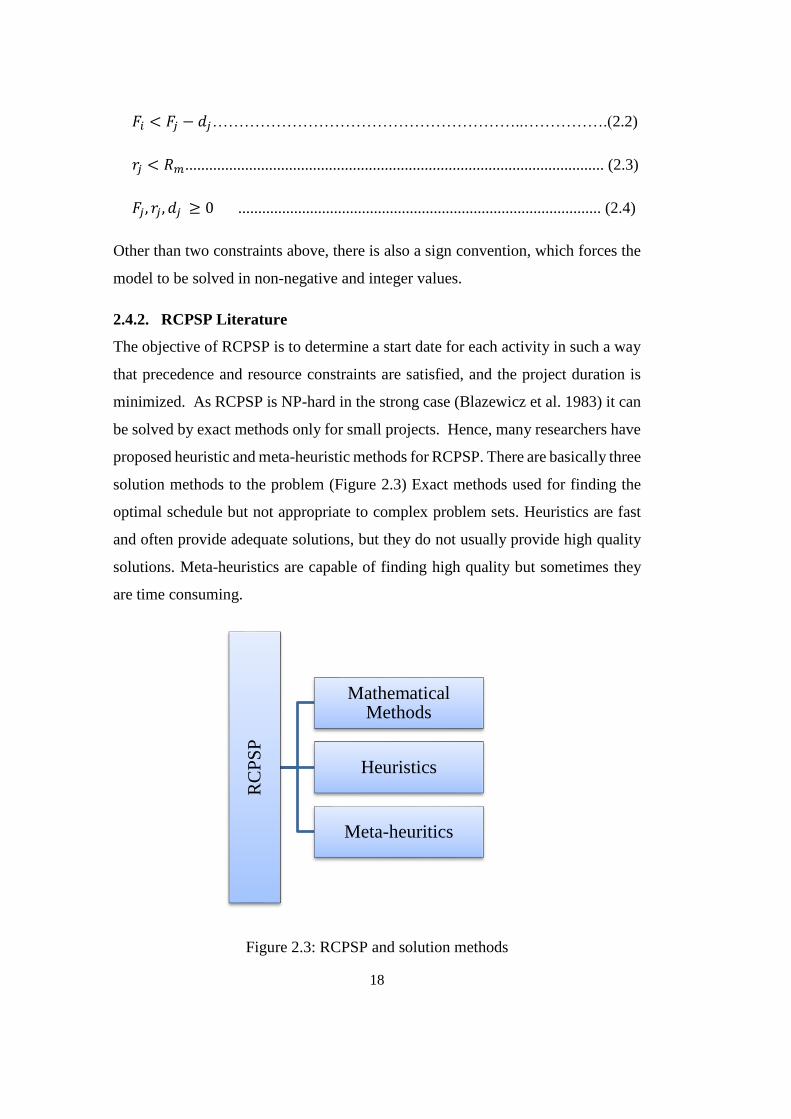
proposed heuristic and meta-heuristic methods for RCPSP. There are basically three
solution methods to the problem (Figure 2.3) Exact methods used for finding the
optimal schedule but not appropriate to complex problem sets. Heuristics are fast
and often provide adequate solutions, but they do not usually provide high quality
solutions. Meta-heuristics are capable of finding high quality but sometimes they
are time consuming.
Figure 2.3: RCPSP and solution methods
RC
PS
P
Mathematical Methods
Heuristics
Meta-heuritics
19
2.4.2.1.Exact Methods
Exact solutions include linear integer programing methods: zero-one programing
and dynamic programing, enumeration; especially branch and bound methods. Very
limited works have been done in term of exact solutions. It is proven that neither
method is computationally feasible for large-sized networks (Kim and Ellis, 2008;
Alcaraz and Maroto, 2001). Kolish et al., (1995) worked on 480 test sets with 30
activities which are soon becoming a standard test set and concluded that 428 of
them can be solved optimally with exact methods, remaining are cannot be solved
even with 1 hour of computation time. Afterwards the researchers concentrated on
52 “hard test sets”. Mingozzi et al., (1995) and their algorithm BBLB3 showed
significant improvements on the optimal solutions, but it was very slow in terms of
computational efficiency.
Pioneering work about zero-one programing approaches are focused on a linear
programming formulation of job-shop scheduling (Pritsker et al., 1969; Patterson
and Roth, 1976). Due dates, job splitting, resource, substitutability, and
concurrency and non-concurrency of job performance requirements are added to
the model and three different objective functions, namely; minimizing the total time
for all projects, minimizing the time by which all projects are completed and
minimizing total lateness or lateness penalty for all projects are researched.
Patterson and Huber (1974) used bounding techniques in conjunction with zero one
programming techniques. Rather than solving one schedule with zero-one
technique, it is intended to examine feasibility of a series of schedules. Its
advantages over simple zero-one programming techniques are compared.
An example of dynamic programming techniques is given at Carruthers and
Battersby (1966). Elmaghraby (1993) investigated the dynamic programming
technique with the assumption that there is a relationship between the amount of
the resources allocated to an activity and its duration. A dynamic programming
optimization procedure and an approximation are given for upper bound solutions.
20
In all of exact solution methods above mentioned branch and bound algorithms
(Christofides et al., 1987; Demeuelemeester and Herroelen, 1992) are very common
in the literature. Branching can be defined as dividing disjoint solution subsets into
subsets (Demeulemeester and Herroelen, p: 220, 2002). Basically, it is a divide and
conquer algorithm in which large problem set cannot be solved directly, instead it
is divided into smaller sub problems that can be conquered. Two actions are
required for the algorithm. The first action is dividing the problem into sub
problems-which is called branching; second action is giving a bound for best
solution in the subset-which is called bounding. Thus, it is a search algorithm to
find the best solution among other solutions available.
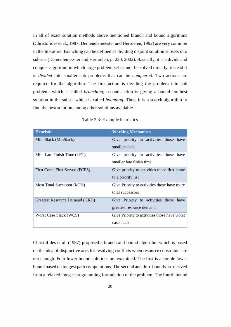
Table 2.3: Example heuristics
Heuristic Working Mechanism
Min. Slack (MinSlack) Give priority to activities those have
smaller slack
Min. Late Finish Time (LFT) Give priority to activities those have
smaller late finish time
First Come First Served (FCFS) Give priority to activities those first come
to a priority list
Most Total Successor (MTS) Give Priority to activities those have more
total successors
Greatest Resource Demand (GRD) Give Priority to activities those have
greatest resource demand
Worst Case Slack (WCS) Give Priority to activities those have worst
case slack
Christofides et al. (1987) proposed a branch and bound algorithm which is based
on the idea of disjunctive arcs for resolving conflicts when resource constraints are
not enough. Four lower bound solutions are examined. The first is a simple lower
bound based on longest path computations. The second and third bounds are derived
from a relaxed integer programming formulation of the problem. The fourth bound
21
is based on the disjunctive arcs used to model the problem as a graph. The report is
done based on the performances of randomly generated sets which involve up to 25
activities and 3 resources.
Demeuelemeester and Herroelen (1992) used a branch-and-bound procedure which
is described for scheduling the activities of a project of the PERT/CPM variety
subjects to precedence and resource constraints where the objective is to minimize
project duration. The procedure is based on a depth-first solution strategy in which
nodes in the solution tree represent the resource and precedence feasible partial
schedules. The procedure is programmed in the C and validated using a standard
set of test problems with between 7 and 50 activities requiring up to three resources.
2.4.2.2.Heuristics
Heuristics are experienced based techniques which have a subroutine applied to
problem solving strategy and generally have adequate solutions in a very short time.
Most heuristics are rules that are tailored to fit for specific types of problems. They
may be deterministic and stochastic whether the same results can be found at each
iteration or not. Some examples can be seen from Table 2.3.
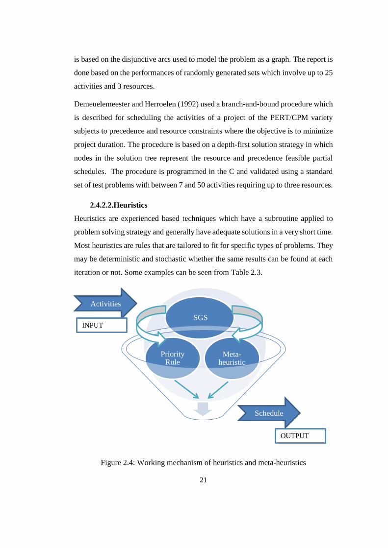
Figure 2.4: Working mechanism of heuristics and meta-heuristics
Meta-heuristic
Priority Rule
SGS
Activities
Schedule
INPUT
OUTPUT
22
Minimum Slack Rule (MinSlack) is generally accepted as an adequate solution for
RCPSP and can be applied with First Come First Served (FCFS) rule as a tie
breaker. Heuristics are important since they offer some upper bounds for those
cannot be solved optimally.
The heuristic studies for the RCPSP date back to Kelley (1963) with a schedule
generation schema (SGS). SGS is at the hearth of heuristics and meta-heuristics as
well as it is a heuristic itself. It starts from zero to build a schedule by stepwise
improvements. There are two different SGS available in the literature. One is based
on activity increment- serial SGS and the other is based on time increment - parallel
SGS. In serial SGS, based on activity selection principle, activities are scheduled at
the earliest possible time under the resource constraints. Nevertheless, at parallel
SGS, for every time increment activities are scheduled under the resource
constraints (Kolish and Hartmann, 1999). In order to build a schedule either SGS is
used together with a priority rule or meta-heuristics. The mechanism is shown at
Figure 2.4. An ordered list is obtained with a priority or a meta-heuristic, the
schedule is configured with SGS
Davis and Patterson (1975) tested various heuristic sequencing rules on RCPSP
with the total project minimization objective function. Effectiveness of heuristics
shown by comparison to optimum solutions available. Minimum Slack Rule
performed best from eight heuristic test with eighty tree problems. It is reported
that, the performance of heuristics was relatively small as resource constraints get
tightened.
Backward forward improvement method (Li and Willis, 1992) is a special
improvement method that is based on scheduling with same SGS and heuristics, in
reverse time direction. In backward scheduling the exact duration of feasible
schedule is not known, an arbitrary completion time is selected and all precedence
relations are reversed. Finally, all activities are scheduled as late as possible
according to activity selection principle. In the same manner resulting schedule can
be scheduled in forward direction according to starting dates as early as possible
23
and final schedule generally be denser and shorter than starting schedule, at least it
has the same duration
Priority-rule-based heuristics (PR-H) use a SGS in order to build a schedule.
Priority rule is used for selecting the nominee activities from the activity set. PR-H
can be classified according to criteria it employs, i.e. network, time and resource
based rules. If PR-H generates a single solution it is called single pass method, if it
generates more than one schedules, it is called multi pass methods (Kolish and
Hartman, 1999). PR-H can be applied to get one solution at a time. As an example
of shown heuristics see Hartman et al. (2000), where Late Finish Time (LFT) and
Worst Case Slack (WCS) rule is used in experiments on test of algorithms
performances.
Some heuristics produce more than one solution and best of them can be selected.
Sampling methods (Cooper, 1976) are examples of this kind of heuristics. The
selection probability of activities from decision set is determined according to a
selection principle and the schedule is constructed upon selection probabilities.
Another method is selecting more than one heuristics in a random manner which
can be found at Storer et al., (1992).
Hartman et al., (2000) conducted an experiment on the performances of heuristic
algorithms by applying an experimental design with control parameters on test sets.
A full experiment design is applied in order to test different heuristics’
performances on standard J sets (Kolish et al., 1999). Influence of increasing
project size, network complexity, resource factor and resource straight is tested.
Worst Case Slack (WCS) and Late Finish Time (LTF) combined with parallel SGS
outperformed other priority rule based heuristics. Meta-heuristics performed better
as schedule number was increased from 1000 to 5000. It was concluded that since
meta-heuristics use knowledge exploited from different schedules, they have
superiority on priority rule based heuristics. It is stated that the selection of SGS
may be influenced by project size since serial SGS performed better in J30 sets
while parallel SGS performed better in J120 sets.
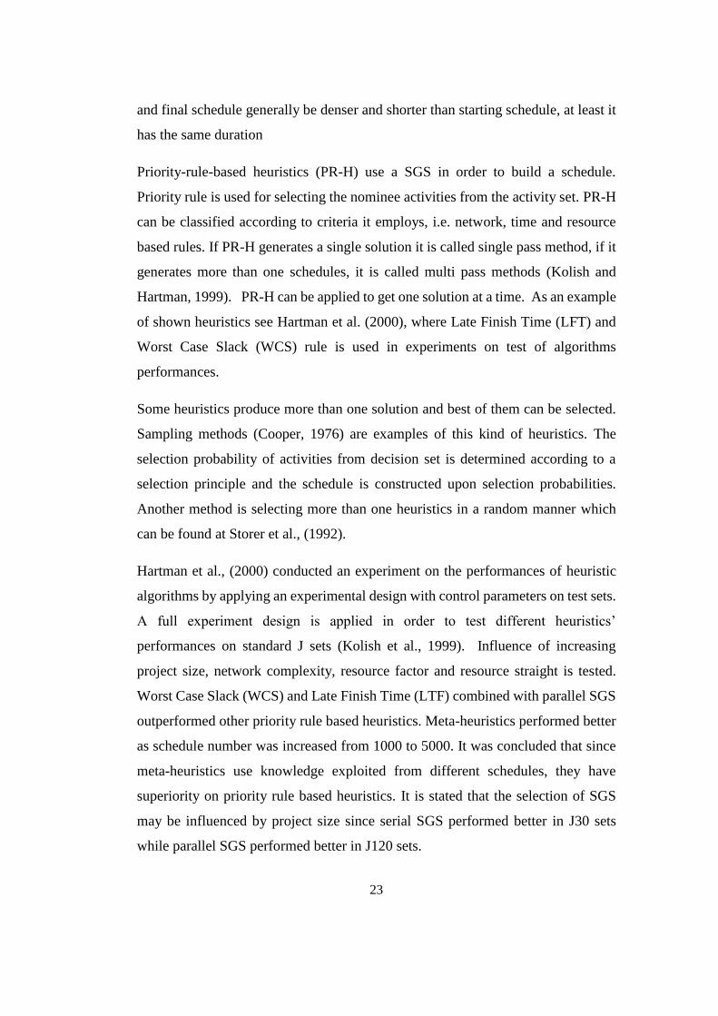
24
Kanit et al., (2009) investigated MinSlack, LFT and Maximum Remaining Path
Length (MRPL) heuristics on the scheduling of housing projects. Tests were
conducted using ten real projects. MRPL rule performed better at six projects, LFT
performed better at three projects and MinSlack rule performed better at one
project. It is suggested that MRPL rule can be used for housing projects with
resource constrained where activity numbers are high.
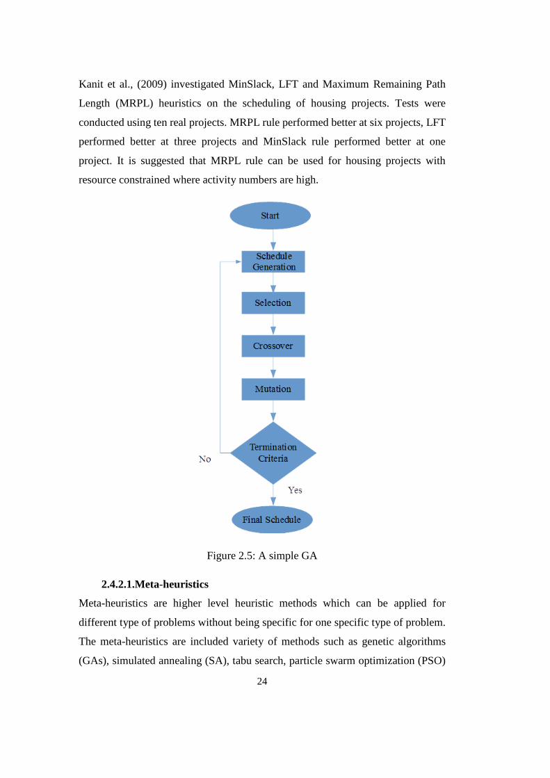
Figure 2.5: A simple GA
2.4.2.1.Meta-heuristics
Meta-heuristics are higher level heuristic methods which can be applied for
different type of problems without being specific for one specific type of problem.
The meta-heuristics are included variety of methods such as genetic algorithms
(GAs), simulated annealing (SA), tabu search, particle swarm optimization (PSO)
25
and ant colony optimization (ACO) which mimic a natural phenomenon in order to
find a global optimum in a large search space.
Among all meta-heuristics, GAs have a large variety of application areas. It is a
population-based and stochastic search algorithm based on evolutionary
computation principles inspired by the Darwinian principles of natural selection
(Holland, 1975). GAs finds for best solution from a pool of solutions according to
some selection and diversification mechanisms as shown at Figure 2.5. A solution
is called individuals where an individual is represented by a chromosome. Number
of solutions constitute a set which is called as a generation.
New solutions are produced depending on previous generations’ chromosomes
according to crossover and mutation operators. The best solutions are given to
higher change to survive and some of them are moved to new generations with
elitism. A fitness function is used in order to evaluate a chromosome’s performance.
What makes GAs strong compared with other algorithms is that it has the ability of
exploiting the best solution while exploring the search space effectively
(Michalewich, p. 15, 1992).
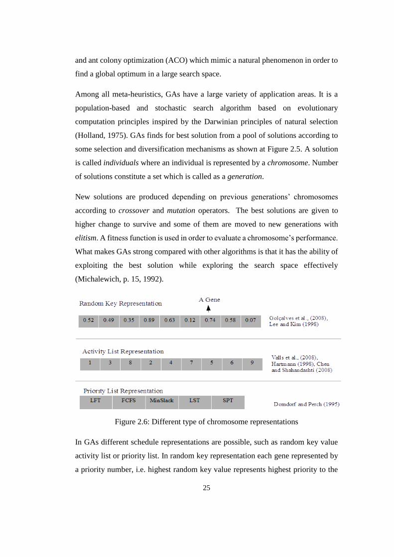
Figure 2.6: Different type of chromosome representations
In GAs different schedule representations are possible, such as random key value
activity list or priority list. In random key representation each gene represented by
a priority number, i.e. highest random key value represents highest priority to the
26
activity. Whereas in an activity list representation, a schedule is represented with
list of activities; order of an activity means it is scheduled prior to others. A priority
list representation is also available where a heuristic is used to choose activities and
chromosome representations show priority of that heuristics. At Figure 2.6 some
examples of different chromosome representations are shown.
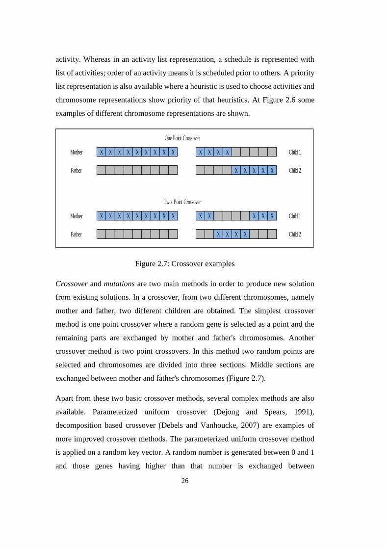
Figure 2.7: Crossover examples
Crossover and mutations are two main methods in order to produce new solution
from existing solutions. In a crossover, from two different chromosomes, namely
mother and father, two different children are obtained. The simplest crossover
method is one point crossover where a random gene is selected as a point and the
remaining parts are exchanged by mother and father's chromosomes. Another
crossover method is two point crossovers. In this method two random points are
selected and chromosomes are divided into three sections. Middle sections are
exchanged between mother and father's chromosomes (Figure 2.7).
Apart from these two basic crossover methods, several complex methods are also
available. Parameterized uniform crossover (Dejong and Spears, 1991),
decomposition based crossover (Debels and Vanhoucke, 2007) are examples of
more improved crossover methods. The parameterized uniform crossover method
is applied on a random key vector. A random number is generated between 0 and 1
and those genes having higher than that number is exchanged between
X X X X X X X X X X X X X
X X X X X
X X X X X X X X X X X X X X
X X X X
Child 1
Child 2
Child 1
Child 2
One Point Crossover
Two Point Crossover
Mother
Father
Mother
Father
27
corresponding mother locations. Decomposition based crossover is started with
determining the weakest resource used regions in a father chromosome and best
resource used regions in a mother's chromosome. Finally, worse parts are replaced
with the better part of father chromosome.
Mutations are applied as a random change of a gene or a number of genes on a
chromosome. Along iterations chromosomes may trap into local minimums. Thus,
the solution may lead a premature convergence, which does not allow reaching of
optimum results. Mutations may lead to skip from local minimums. Generally
mutation ratio is too small since too many mutant genes may also avoid to converge
(Yang, p: 25, 2008).
Hartmann (1998) studied RCPSP with makespan minimization objective. A new
GA is proposed and it has been compared with two other GAs. Starting with the
empty job sequence list, preceding activities are selected randomly from an
unselected activity set. In addition, a known sampling method and a priority rule
are used to derive activity selection probabilities. Results were compared with two
known GAs and some heuristics.
Leu and Hwang (2001) studied RCPSP in a repetitive construction project- precast
production. It is stated that line of balance method (LOB) is not sufficiently enough
to solve scheduling problems under resource constraint. In the paper random key
representation is used along with GA. Influencing factors of the repetitive precast
production scheduling model and their impacts were examined. Results revealed
that GAs are very efficient in precast production scheduling.
Leu and Yang (1999) proposed a GA based scheduling system called GARCS. A
new crossover and mutation is shown and its effectiveness was tested on problem
instances.
Chen and Weng (2009) proposed a two-phase GA in which both the effects of time-
cost trade-off and resource scheduling are combined in order to get the best result
for RCPSP. A GA based time-cost trade-off analysis is used to select the execution
28
mode of each activity and it is followed by other GA-based resource scheduling
method.
Chen et al. (2010) proposed a hybrid algorithm called as ACOSS which combines
a local search strategy, ant colony optimization, and a scatter search in an iterative
process.
In recent years, other than RCPSP there has been an increasing interest in the
adaptation of GAs to optimization problems in construction engineering and
management. Multi-mode RCPSP (Mori and Tseng, 1997), resource leveling
(Hegazy 1999, El-Rayes and Jun 2009), planning of construction resource
utilization (Kandil and El-Rayes 2006; Kandil et al. 2010), planning of post disaster
temporary housing projects (Kandil et al. 2010), time-cost tradeoff problem (Feng
et al. 1997; Kandil and El-Rayes 2005), and time-cost-quality trade-off (Kandil and
El-Rayes 2005) are among the construction management problems in which GAs
are proposed.
Simulated annealing (SA) has fine tuning capabilities, and is usually capable of
escaping of local optima for locating a good approximation to the global optimum
(Hwang and He, 2006). But a sole SA has a low search efficiency as it maintains
one solution at a time. It was applied in the optimization problem by Kirkpatrick et
al., (1983). It mimics the annealing process of materials. The basic idea behind the
algorithm is to use a randomized search technique with accepting worse solutions
to some extent. In the early stages of the algorithm the probability of accepting
worse solutions is high. This acceptance probability is reduced in a cooling schema
where probability is:
𝑝 = 𝑒−∆𝐸
𝑘𝑇……………………………………………………………………. (2.5)
where ∆E is the rate of change in the objective function, T is temperature and k is
Boltzmann’s constant. A flow chart of the basic SA algorithm is given at Figure
2.8.
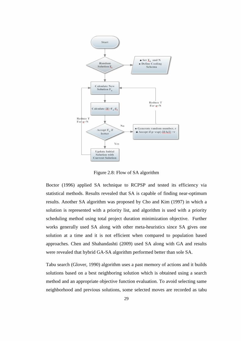
29
Figure 2.8: Flow of SA algorithm
Boctor (1996) applied SA technique to RCPSP and tested its efficiency via
statistical methods. Results revealed that SA is capable of finding near-optimum
results. Another SA algorithm was proposed by Cho and Kim (1997) in which a
solution is represented with a priority list, and algorithm is used with a priority
scheduling method using total project duration minimization objective. Further
works generally used SA along with other meta-heuristics since SA gives one
solution at a time and it is not efficient when compared to population based
approaches. Chen and Shahandashti (2009) used SA along with GA and results
were revealed that hybrid GA-SA algorithm performed better than sole SA.
Tabu search (Glover, 1990) algorithm uses a past memory of actions and it builds
solutions based on a best neighboring solution which is obtained using a search
method and an appropriate objective function evaluation. To avoid selecting same
neighborhood and previous solutions, some selected moves are recorded as tabu

30
list. The iteration continues until a stopping criteria is met (Thomas and Salhi,
1998). Due to use of memory and record of past actions, algorithm could save
computing time and can increase the efficiency significantly (Yang, p. 92, 2008).
The mechanism of the algorithm in RCPSP works such as; an initial feasible
solution is obtained and this solution is disturbed with a move function and finally
a new solution is obtained.
Lee and Kim (1996) used random solution for initial solutions and neighborhood
generation method for new solutions. They selected activities from previous four
and next four activities randomly in neighborhood search mode. Tabu list is
obtained by defining tabu moves such as interchanging priorities of activities i and
j, if activities are interchanged recently.
Icmeli and Erenguç (1994) used tabu search algorıthm on RCPSP with discounted
cash flows. The method was tested on 50 problems derived from Patterson's data
set. Solutions were compared with upper bound results and MinSlack rule used
solutions.
Particle Swarm Optimization (PSO) is another evolutionary technique that mimics
the behaviors of birds flocking. It starts with an initial solution and looks for
solution in the search space by iterations. Unlike GAs, PSO does not use
evolutionary operators. The particles follow its paths one by one with its good
experiences. For n particles there would be n current best solutions. The aim is to
find globally best solution compared with current solutions.
Jia and Seo (2013) proposed an improved PSO method which treats the solutions
of RCPSP as particle swarms and employs a double justification skill. It uses
operator for the particles, in association with rank-priority-based representation,
greedy random search, and serial scheduling scheme.
Ant Colony Optimization (ACO) is another meta-heuristic method that mimics the
behaviors of ants looking for best foraging paths. Ants that find foods mark it with
a chemical (pheromone) in order to be trailed by other ants. Those ants following
same route improves the chemical concentration. As more ants follow the same
31
route, the route becomes a favorable one. It gives a feedback for those ants which
start to find food sources.
Merkle et al., (2002) proposed an ACO method for RCPSP. Proposed method uses
combinations of two pheromone evaluation methods to find new solutions, these
are: a change of the influence of the heuristic on the decisions of the ants during the
run of the algorithm, and the option that an elitist ant forgets the best-found solution.
Tseng and Chen (2006) proposed a hybrid approach called ANGEL, which
combines (ACO), (GA) and a local search strategy together. In this method first,
ACO searches the solution space and generates the initial population for GA. Next,
GA is executed and the pheromone set in ACO is updated when GA obtains a better
solution. When GA terminates, ACO searches again by using a new pheromone set.
ACO and GA search alternately and cooperatively in the solution space. Finally a
local search strategy fine tunes the results of ACO and GA.
2.5.Resource Constrained Multi-Project Scheduling Problem (RCMPSP)
2.5.1. Problem Definition
The resource constrained multi-project scheduling problem (RCMPSP) is an
extension of the RCPSP and consists of simultaneous scheduling of two or more
projects with common resource constraints, while minimizing some performance
measure. It is quite often that managers deal with more than one projects in practical
cases (Browning and Yassine, 2010). Payne (1995) states that %90 of the projects
are carried out in a multi-project context. Lova et al., (2000) made a survey in
construction, textile, IT and public administration sectors about the project
environment. %84 of correspondents answered that they work in a multi-project
environment. Same survey concluded that project scheduling software programs are
not practical to manage multi-projects and they should be adapted to this need.
These survey results reveal that multi-project environment is a more practical and
common case compared with a single project for scheduling purposes.
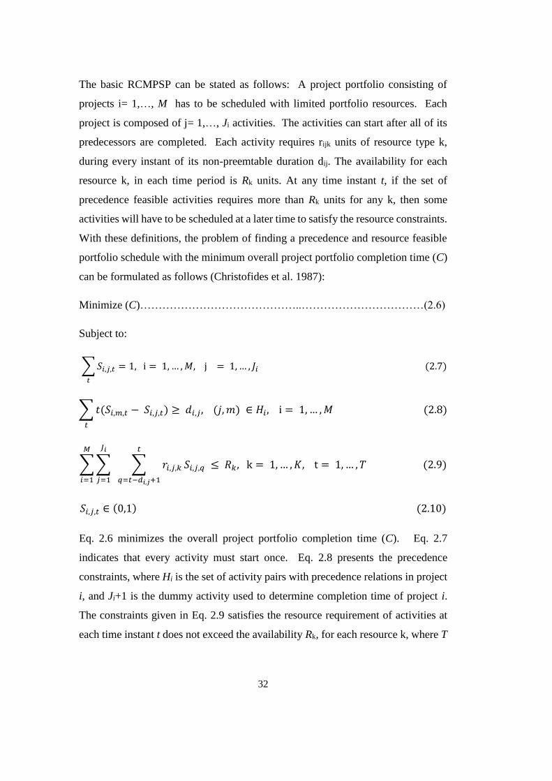
32
The basic RCMPSP can be stated as follows: A project portfolio consisting of
projects i= 1,…, M has to be scheduled with limited portfolio resources. Each
project is composed of j= 1,…, Ji activities. The activities can start after all of its
predecessors are completed. Each activity requires rijk units of resource type k,
during every instant of its non-preemtable duration dij. The availability for each
resource k, in each time period is Rk units. At any time instant t, if the set of
precedence feasible activities requires more than Rk units for any k, then some
activities will have to be scheduled at a later time to satisfy the resource constraints.
With these definitions, the problem of finding a precedence and resource feasible
portfolio schedule with the minimum overall project portfolio completion time (C)
can be formulated as follows (Christofides et al. 1987):
Minimize (C)……………………………………..……………………………(2.6)
Subject to:
∑ 𝑆𝑖,𝑗,𝑡
𝑡
= 1, i = 1, … , 𝑀, j = 1, … , 𝐽𝑖 (2.7)
∑ 𝑡(𝑆𝑖,𝑚,𝑡 − 𝑆𝑖,𝑗,𝑡) ≥ 𝑑𝑖,𝑗, (𝑗, 𝑚) ∈ 𝐻𝑖, i = 1, … , 𝑀
𝑡
(2.8)
∑ ∑ ∑ 𝑟𝑖,𝑗,𝑘
𝑡
𝑞=𝑡−𝑑𝑖,𝑗+1
𝐽𝑖
𝑗=1
𝑀
𝑖=1
𝑆𝑖,𝑗,𝑞 ≤ 𝑅𝑘, k = 1, … , 𝐾, t = 1, … , 𝑇 (2.9)
𝑆𝑖,𝑗,𝑡 ∈ (0,1) (2.10)
Eq. 2.6 minimizes the overall project portfolio completion time (C). Eq. 2.7
indicates that every activity must start once. Eq. 2.8 presents the precedence
constraints, where Hi is the set of activity pairs with precedence relations in project
i, and Ji+1 is the dummy activity used to determine completion time of project i.
The constraints given in Eq. 2.9 satisfies the resource requirement of activities at
each time instant t does not exceed the availability Rk, for each resource k, where T
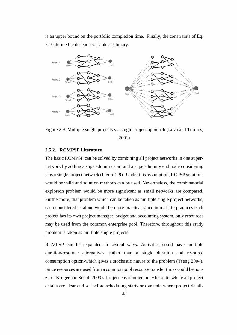
33
is an upper bound on the portfolio completion time. Finally, the constraints of Eq.
2.10 define the decision variables as binary.
Figure 2.9: Multiple single projects vs. single project approach (Lova and Tormos,
2001)
2.5.2. RCMPSP Literature
The basic RCMPSP can be solved by combining all project networks in one super-
network by adding a super-dummy start and a super-dummy end node considering
it as a single project network (Figure 2.9). Under this assumption, RCPSP solutions
would be valid and solution methods can be used. Nevertheless, the combinatorial
explosion problem would be more significant as small networks are compared.
Furthermore, that problem which can be taken as multiple single project networks,
each considered as alone would be more practical since in real life practices each
project has its own project manager, budget and accounting system, only resources
may be used from the common enterprise pool. Therefore, throughout this study
problem is taken as multiple single projects.
RCMPSP can be expanded in several ways. Activities could have multiple
duration/resource alternatives, rather than a single duration and resource
consumption option-which gives a stochastic nature to the problem (Tseng 2004).
Since resources are used from a common pool resource transfer times could be non-
zero (Kruger and Scholl 2009). Project environment may be static where all project
details are clear and set before scheduling starts or dynamic where project details
34
are changed trough execution. Although the basic RCMPSP has certain practical
limitations such as the assumption of a single duration/resource mode for activities,
or the assumption that resources can be transferred between projects without any
expense in time and cost, the majority of the research on resource constrained multi-
project scheduling have studied the basic problem. In this research, we have focused
on the basic RCMPSP since the majority of the multi-project problem instances
available in the literature include basic RCMPSPs, and commonly used project
management software such as Microsoft Project 2010 can only solve the basic
problem. It can be seen from the literature that while the majority of projects is
scheduled on a multi-project environment, most research on resource-constrained
project scheduling have focused on single projects (Kurtulus and Davis 1982;
Krüger and Scholl 2009; Browning and Yassine 2010). Therefore, in multi project
environment there exists less number of researches. Following section summarizes
the works done in the multi project environment.
2.5.2.1.Exact Methods
Since RCMPSP is a generalization of the RCPSP, it is also NP-hard (Golçalves et
al., 2008). Although exact methods were proposed in the literature, previous studies
have mainly attempted to develop efficient heuristics and meta-heuristics for the
solution of RCMPSP.
Some exact solution methods such as zero-one programming approach (Pritsker et
al., 1969) are proposed in the literature which is unable to solve large instances.
Another example of exact methods is Drexl (1991), in his work a branch and bound
algorithm together with dynamic programming model is proposed. The models and
assumptions under exact models of RCPSP are valid for RCMPSP. Since the project
sizes are larger, exact methods is not practical to use. Further attempt to solve the
problem by exact solution methods are limited with the NP-Hard characteristics of
the problem. Therefore, due to the combinatorial explosion problem many studies
focused on heuristics and meta-heuristics.
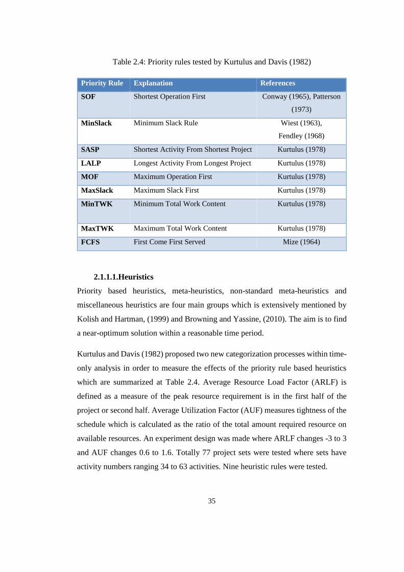
35
Table 2.4: Priority rules tested by Kurtulus and Davis (1982)
Priority Rule Explanation References
SOF Shortest Operation First Conway (1965), Patterson
(1973)
MinSlack Minimum Slack Rule Wiest (1963),
Fendley (1968)
SASP Shortest Activity From Shortest Project Kurtulus (1978)
LALP Longest Activity From Longest Project Kurtulus (1978)
MOF Maximum Operation First Kurtulus (1978)
MaxSlack Maximum Slack First Kurtulus (1978)
MinTWK Minimum Total Work Content Kurtulus (1978)
MaxTWK Maximum Total Work Content Kurtulus (1978)
FCFS First Come First Served Mize (1964)
2.1.1.1.Heuristics
Priority based heuristics, meta-heuristics, non-standard meta-heuristics and
miscellaneous heuristics are four main groups which is extensively mentioned by
Kolish and Hartman, (1999) and Browning and Yassine, (2010). The aim is to find
a near-optimum solution within a reasonable time period.
Kurtulus and Davis (1982) proposed two new categorization processes within time-
only analysis in order to measure the effects of the priority rule based heuristics
which are summarized at Table 2.4. Average Resource Load Factor (ARLF) is
defined as a measure of the peak resource requirement is in the first half of the
project or second half. Average Utilization Factor (AUF) measures tightness of the
schedule which is calculated as the ratio of the total amount required resource on
available resources. An experiment design was made where ARLF changes -3 to 3
and AUF changes 0.6 to 1.6. Totally 77 project sets were tested where sets have
activity numbers ranging 34 to 63 activities. Nine heuristic rules were tested.
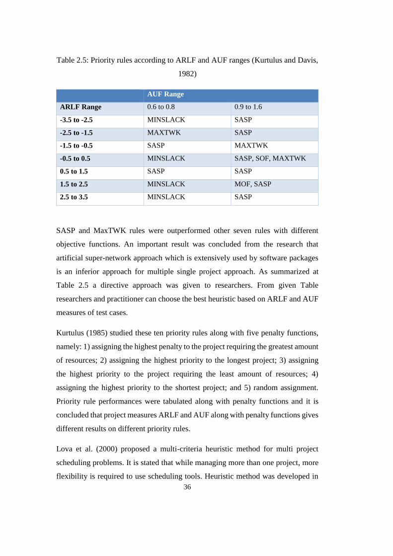
36
Table 2.5: Priority rules according to ARLF and AUF ranges (Kurtulus and Davis,
1982)
AUF Range
ARLF Range 0.6 to 0.8 0.9 to 1.6
-3.5 to -2.5 MINSLACK SASP
-2.5 to -1.5 MAXTWK SASP
-1.5 to -0.5 SASP MAXTWK
-0.5 to 0.5 MINSLACK SASP, SOF, MAXTWK
0.5 to 1.5 SASP SASP
1.5 to 2.5 MINSLACK MOF, SASP
2.5 to 3.5 MINSLACK SASP
SASP and MaxTWK rules were outperformed other seven rules with different
objective functions. An important result was concluded from the research that
artificial super-network approach which is extensively used by software packages
is an inferior approach for multiple single project approach. As summarized at
Table 2.5 a directive approach was given to researchers. From given Table
researchers and practitioner can choose the best heuristic based on ARLF and AUF
measures of test cases.
Kurtulus (1985) studied these ten priority rules along with five penalty functions,
namely: 1) assigning the highest penalty to the project requiring the greatest amount
of resources; 2) assigning the highest priority to the longest project; 3) assigning
the highest priority to the project requiring the least amount of resources; 4)
assigning the highest priority to the shortest project; and 5) random assignment.
Priority rule performances were tabulated along with penalty functions and it is
concluded that project measures ARLF and AUF along with penalty functions gives
different results on different priority rules.
Lova et al. (2000) proposed a multi-criteria heuristic method for multi project
scheduling problems. It is stated that while managing more than one project, more
flexibility is required to use scheduling tools. Heuristic method was developed in
37
order to account for two criteria, one is project splitting and other is mean project
delay. Heuristic work is given in two phases: in the first phase iterative forward-
backward process is used with mean project delay objective function. In the second
phase, results is improved with no time criteria. MaxTWK and MinLFT priority
rules were the bet rules that dominate others under different criteria.
Lova and Tormos (2001) studied the effect of the SGS – serial or parallel – and
priority rules – MinLFT, MinSLK, MaxTWK, SASP or FCFS – with two
approaches – multi-project and single-project under mean project delay objective.
A two stage iterative process is proposed where in the first stage priority is given to
a project, in the second stage activities are selected with heuristics. It is stated that
P-SGS found better results performing under mean project delay objective
functions.
Lova and Tormos (2002) further examined the two stage project selection principle
with other possibilities of selecting SGS and other multi-pass heuristics. A new
hybrid heuristic method combining random sampling and forward backward
iteration is given.
Krüger and Scholl (2009) studied the problem under resource transfer times. In this
model resources transferred to another project is modelled. Sequence and resource
dependent transfer time constraints are added to the model which represent setup
times for activities when a resource is removed from one project and reassigned to
another. It is concluded that commonly accepted static environment assumption and
static nature of portfolio cannot represent real life problems. Resource transfer
times should be included in the models despite the models may include more
comprehensive work.
Browning and Yassine (2010) studied RCMPSP with its two lateness objectives-
project lateness and portfolio lateness. Five measures of RCMPSP characteristics
are used along with a full factorial experiment on 12,320 randomly generated
problem instances. A directive tool is given for a manager to choose which priority
rule is best under selected project network.
38
2.1.1.2.Meta-heuristics
Focusing on the main objective of this thesis it can be seen that meta-heuristic
studies are primarily aiming to solve RCPSP. Particle swarm optimization (Jarboui
et al. 2008; Wang and Qi 2009; Chen 2011; Jia and Seo, 2013), ant colony
optimization (Merkle et al. 2002; Tseng and Chen, 2006), simulated annealing (Cho
and Kim, 1997; Hwang and He, 2006), honey-bee mating optimization (Bozorg
Haddad et al. 2010; Akbari et al. 2011), hybrid GA and SA (Bettemir and Sönmez,
2014) and tabu search algorithm (İçmeli and Erenguç, 1994; Lee and Kim, 1996)
are the main studies aiming to solve RCPSP. There is also particular interest for
GAs such as (Lee and Kim 1996; Hartmann 1998; Leu and Yang 1999; Leu and
Hwang 2001; Toklu 2002; Kim and Ellis 2008; Cheng and Weng 2009; Lin et al.
2013).
Majority of the studies with extensive literature is focusing on RCPSP. Being a
more practical case, RCMPSP has not drown the attention of researches yet. Very
limited research was proposed in the literature. One of them is a sole genetic
algorithm along with a priority rule which is proposed by Kumanan et al. (2006). A
GA is used to select the sequence of projects where priority rule is used for
scheduling within projects. The proposed method outperformed other heuristics
such as FCFS and SPT.
A multi-agent systems (Confessore et al., 2007) is proposed within a decentralized
multi project problem. In the model agents are used to communicate with project
managers and portfolio manager.
Gonçalves et al., (2008) proposed a GA with random key representation. In order
to capture real practices, model were capable of integrating due dates, work in
process, and inventory. Constraints enforcing the release date concept are also
introduced.
A hybrid meta-heuristic was proposed by Chen and Shahandashti (2009) where GA
and SA approaches combined together to give better results. SA approach was
39
integrated to model in order to improve GA’s search capacity with accepting worse
solutions.
Within above aforementioned limited works, it can be said that there is a significant
research potential for RCMPSP. Meta-heuristics have high potential to solve the
RCMPSP.
2.6. Parallel Computing Literature on Meta-heuristics
2.6.1. Introduction
Different from parallel computing, serial computing is the usual computing, which
engineers have been using for 50 years. In this type of computing instructions given
to the computer is running one after another and speed of the computation relies on
the central processing unit (CPU) clock speed. Traditional computers’ CPUs follow
Moore’s Law, which describes a long-term trend in the history of computing
hardware. According to this law, the number of transistors that can be placed on an
integrated circuit has doubled approximately every two years. The trend has
continued for more than half a century and is not expected to stop (Arenas et al.,
2011). Nevertheless, physically CPUs has reached its limits. This resulted in a new
era of computing, which called parallel is computing. In parallel computing,
instructions can be run on different cores at the same time. It makes possible to
increase applications’ effectiveness.
Although as end users, we are not aware of the parallel computing era, it has already
been started and incorporated with many devices. Electronic devices, multi-core
PCs, cell phones have all had parallel computing capabilities. Due to the limits of
current processor clock speed, it is expected that parallel computing will be the new
era of computers. Therefore, possible parallel computing applications would bring
new opportunities to the engineers and end users such that faster applications,
robust calculations and low cost of computing.
Although GAs are effective in solving many optimızation problems in science,
engineering, and business applications, longer execution time to compute each
fitness value of the problem limits its performance. Due to the subroutine of the
40
algorithm, for each cycle time one fitness calculation is possible. Considering the
huge amount of data computation together with several iterations, GAs built
solutions in a considerable time. An approach to use several distributed computers
together for calculation makes it possible to speed up this computation process. One
of the main examples of this process can be seen from Kandil and El-Rayes (2006).
The main objective of Kandil and El-Rayes (2006) work is to develop a parallel
multi-objective genetic algorithm framework that is capable of distributing the
computations over a network of computers. Five research questions are examined.
These are;
Can parallel GAs enable an efficient optimization of large-scale projects?
What are the time savings achieved?
How many processors are needed?
What is the effect of parallel GA design on efficiency and effectiveness?
Which parallel GA paradigm is more suitable for optimization large-scale
projects?
Two parallelism approach was applied namely the global parallel GA and coarse-
grained GA. In the first approach a main processors is selected in charge of all
others and other processors are used for fitness evaluation. In the second approach,
the global population is divided into sub-populations called demes that are evolved
independently. A migration process is applied where best solutions are exchanged
within clusters. Results of first approach revealed a time saving of 7.14 times for
720 activities network. In the second approach three different sized large-scale
construction project is selected that contains 180, 360 and 720 activities as test
cases. Elapsed time for 180 activities network in one processors was 4 hours and it
significantly reduced to 0.5 hours with 5 processors (8 times). Nevertheless,
computation time of 5 processors and 50 processors was almost same and it was not
possible to speed up the computations. In the similar manner, for 360 activities
network almost 8 times speed up was possible up to 5 processors and increasing the
processors beyond 5 did not decrease the computation time. One of the best results
of this study was it is shown that computational time savings are possible. Adding
41
more processors although do not increase computational time beyond 5 to 10
processors, it can increase the quality of the solutions with applied coarse-grained
model. Global parallel GA approach was found as more efficient but less effective
way of parallelism compared to coarse-grained model.
Nevertheless, these networked computers are not easy to manage, requires more
resource and they are expensive. Some researchers use different platforms in order
to search solution space more effectively. A low cost computing device which is
called a Graphical Processing Unit (GPU) is also used by researchers in order to
increase effectiveness of algorithms together with meta-heuristics.
A GPU is a device which has multiple cores on it and used for parallel computing
purposes. It can be programmed with less programing knowledge, it has low initial
and maintenance cost and ease of use together with personal computers make them
suitable for general purpose computing.
2.6.2. Literature Review of GPU Applications
Although GAs are very effective in searching solutions within a domain, crossover,
mutation and selection process requires considerable time. For every population
that has to be evaluated, fitness value should be calculated. Traditional computing
technique is the evaluation of each fitness value at each cycle time of the computer.
Fortunately, GAs are suitable for distributing the computational load to different
cores (Paz and Goldberg, 2000). At this point parallel computing technology brings
new opportunities. There are three different parallelism approaches available in the
literature. These are: master-slave model, fine-grained model and island model
(coarse-grained). With these models it is possible to design different types of GAs.
The master - slave model includes one population but fitness evaluations are
distributed among different cores (Figure 2.10). This model has many advantages:
they explore the search space as a serial GA, it is easy to implement, and it has
several significant improvements in performance (Pospichal et al., 2010). In fine-
grained model it is assumed that any individual can only mate with individuals
located on the neighboring processing nodes. Whereas island model includes more
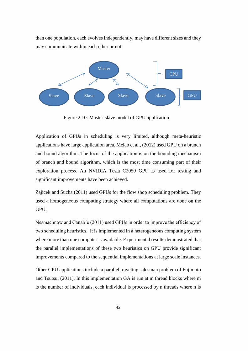
42
than one population, each evolves independently, may have different sizes and they
may communicate within each other or not.
Application of GPUs in scheduling is very limited, although meta-heuristic
applications have large application area. Melab et al., (2012) used GPU on a branch
and bound algorithm. The focus of the application is on the bounding mechanism
of branch and bound algorithm, which is the most time consuming part of their
exploration process. An NVIDIA Tesla C2050 GPU is used for testing and
significant improvements have been achieved.
Zajicek and Sucha (2011) used GPUs for the flow shop scheduling problem. They
used a homogeneous computing strategy where all computations are done on the
GPU.
Nesmachnow and Canab´e (2011) used GPUs in order to improve the efficiency of
two scheduling heuristics. It is implemented in a heterogeneous computing system
where more than one computer is available. Experimental results demonstrated that
the parallel implementations of these two heuristics on GPU provide significant
improvements compared to the sequential implementations at large scale instances.
Other GPU applications include a parallel traveling salesman problem of Fujimoto
and Tsutsui (2011). In this implementation GA is run at m thread blocks where m
is the number of individuals, each individual is processed by n threads where n is
Master
Slave Slave Slave Slave
CPU
GPU
Figure 2.10: Master-slave model of GPU application

43
the number of cities and each thread block performs special crossover and mutation
operators at the same time.
A parallel ant colony optimization is proposed by Delevacq et al., (2013). Max–
Min Ant System (MMAS) algorithm augmented with 3-opt local search is used as
a framework for the implementation of the parallel ants and significant
improvements have been achieved in term of the efficiency of algorithms.
44
CHAPTER 3
3. SOLUTION METHODS
This chapter includes the proposed algorithms for the RCMPSP. First of all, a
mathematical formulation is given. After that, the problem is solved with four
heuristics, a sole GA, a sole SA, a hybrid GA-SA algorithm and a backward forward
hybrid GA-SA. In the last section, algorithm is tested on a Graphical Processing
Unit (GPU) through which it is intended to increase the efficiency of the algorithm.
Test instances, algorithm details and performance of each algorithm is given in
corresponding sections. Throughout the study, a new hybrid algorithm is developed.
GPU implementation of GA is also one of the first research efforts in scheduling
practices.
Mathematical model, heuristics and each meta-heuristic are tested with generated
test instances. In addition, RESCON (Deblaere et al., 2011) and MS Project
heuristics are used for comparison purposes. For small test instance RESCON can
obtain optimum results and its meta-heuristic algorithm is accepted as a successful
method in the literature. Since MS Project’s two heuristics namely standard order
and ID order heuristics are commonly used in practice, it is an important test to see
the capacity of tools available in practice and compare them with developed
algorithm.
3.1.Test Instances
Standard Kolish (Kolisch and Sprecher, 1997) test instances which are J30, J60 and
J120 sets are used for testing purposes. These test instances are extensively used in
literature and commonly accepted for comparison purposes. Percent deviation from
optimum results are given if an optimum result is available. Otherwise lower bound
(CPM based) solutions are used for comparison.
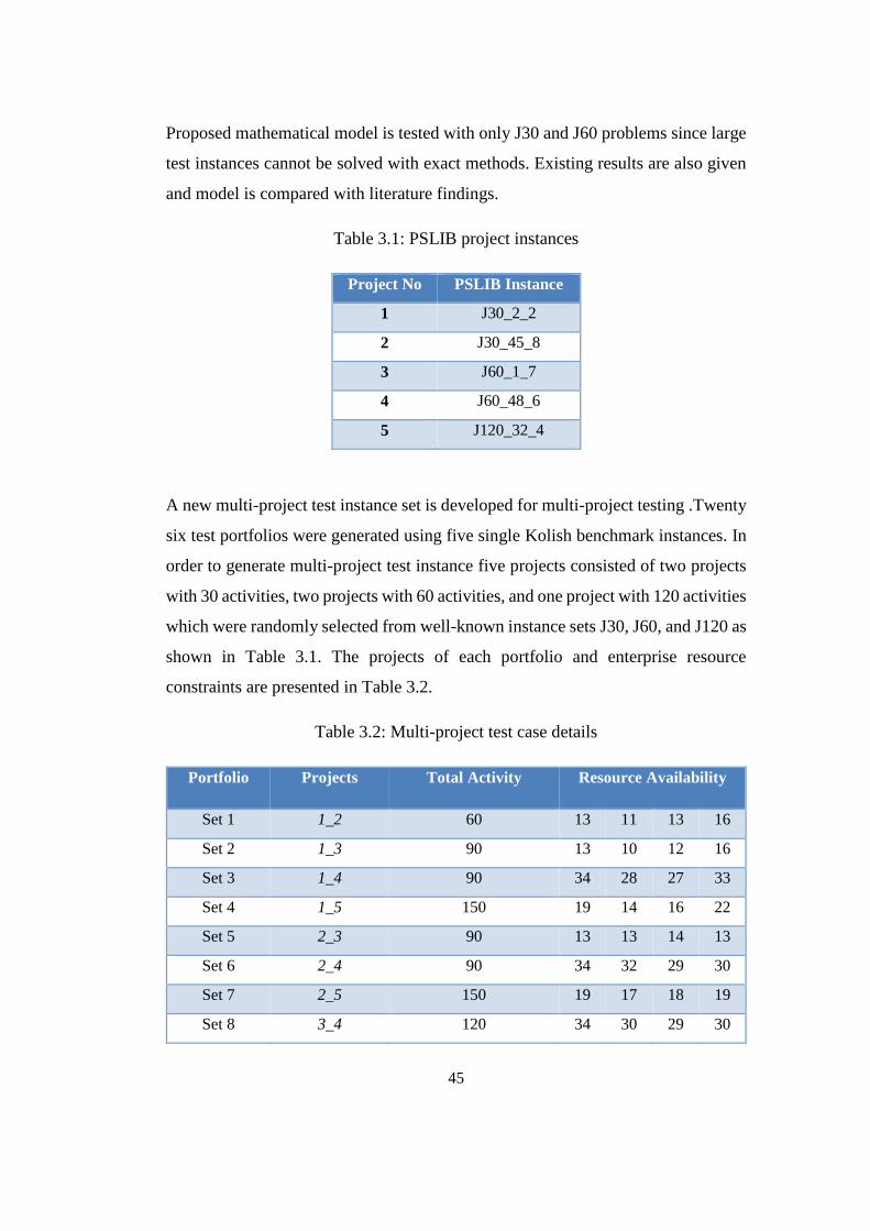
45
Proposed mathematical model is tested with only J30 and J60 problems since large
test instances cannot be solved with exact methods. Existing results are also given
and model is compared with literature findings.
Table 3.1: PSLIB project instances
Project No PSLIB Instance
1 J30_2_2
2 J30_45_8
3 J60_1_7
4 J60_48_6
5 J120_32_4
A new multi-project test instance set is developed for multi-project testing .Twenty
six test portfolios were generated using five single Kolish benchmark instances. In
order to generate multi-project test instance five projects consisted of two projects
with 30 activities, two projects with 60 activities, and one project with 120 activities
which were randomly selected from well-known instance sets J30, J60, and J120 as
shown in Table 3.1. The projects of each portfolio and enterprise resource
constraints are presented in Table 3.2.
Table 3.2: Multi-project test case details
Portfolio Projects Total Activity Resource Availability
Set 1 1_2 60 13 11 13 16
Set 2 1_3 90 13 10 12 16
Set 3 1_4 90 34 28 27 33
Set 4 1_5 150 19 14 16 22
Set 5 2_3 90 13 13 14 13
Set 6 2_4 90 34 32 29 30
Set 7 2_5 150 19 17 18 19
Set 8 3_4 120 34 30 29 30
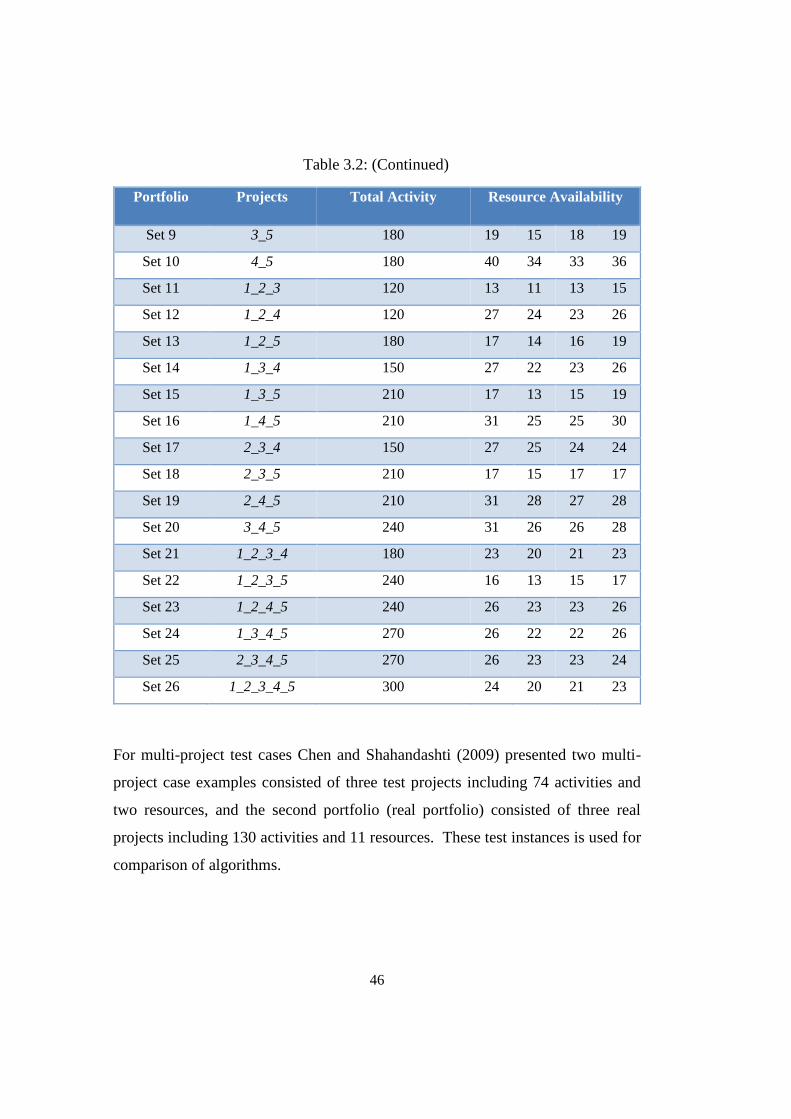
46
Portfolio Projects Total Activity Resource Availability
Set 9 3_5 180 19 15 18 19
Set 10 4_5 180 40 34 33 36
Set 11 1_2_3 120 13 11 13 15
Set 12 1_2_4 120 27 24 23 26
Set 13 1_2_5 180 17 14 16 19
Set 14 1_3_4 150 27 22 23 26
Set 15 1_3_5 210 17 13 15 19
Set 16 1_4_5 210 31 25 25 30
Set 17 2_3_4 150 27 25 24 24
Set 18 2_3_5 210 17 15 17 17
Set 19 2_4_5 210 31 28 27 28
Set 20 3_4_5 240 31 26 26 28
Set 21 1_2_3_4 180 23 20 21 23
Set 22 1_2_3_5 240 16 13 15 17
Set 23 1_2_4_5 240 26 23 23 26
Set 24 1_3_4_5 270 26 22 22 26
Set 25 2_3_4_5 270 26 23 23 24
Set 26 1_2_3_4_5 300 24 20 21 23
For multi-project test cases Chen and Shahandashti (2009) presented two multi-
project case examples consisted of three test projects including 74 activities and
two resources, and the second portfolio (real portfolio) consisted of three real
projects including 130 activities and 11 resources. These test instances is used for
comparison of algorithms.
Table 3.2: (Continued)

47
3.2. A Mathematical Formulation of RCPSP
Since mathematical model gives insight behavior of the problem itself, a
mathematical model is given in this section. Considering the previous works
mathematical model of the problem is regenerated for this problem is as follows;
A finite set which includes activities },,2,1{ nN and activity relations
}, :),{( NjijiA is given. If Aji ),( that means activity j cannot start before
i is finished. In addition, resources Kk is given, the availability of resource k is
shown as kR and resource usage of activity j is defined as kjr , (
kkj Rr ,0 )
3.2.1. Parameters
),( ANG Graph with arcs and activities
},,2,1{ nN Activities
}, ),{( NjijiA Precedence set
K: Type of resource Kk ,,2,1
:kR Resource limits of k
r j,k : Resource usage of activity j from resource k
:ip Processing time of activity i
:M A large number
3.2.2. Variables
:is i start time of task i
:ic Finish time of task i
:maxC Finish time of last dummy activity,

48
:, jix If start time of task i is smaller than finish time of task j than 1, jix ,
otherwise 0, jix . That is;
..,0
,1,
wo
csx
ji
ji
:, jih If start time of task i is larger or equal than start time of task j 1, jih ,
otherwise 0, jih . That is:
0..
1,
wo
ssh
ij
ji
:, jiz If start time of task i is between the start time and finish time of task j
1, jiz , otherwise 0, jiz . That is:
0..
1,
wo
cssz
jij
ji
Where binary variables jiy ,,
jit ,}1,0{
3.2.3. Constraints
iij sps
Aji ),( (3.1)
iii spc
Ni (3.2)
icC max Ni (3.3)
jiji yMcs ,*
Aji ),( and ji (3.4)
)1(*1 ,, jiji yMx
Aji ),( and ji (3.5)
jiji tMss ,*1 Aji ),( and ji (3.6)
)1(*1 ,, jiji tMh Aji ),( and ji
(3.7)
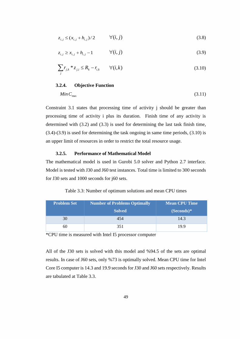
49
2/)( ,,, jijiji hxz
),( ji
(3.8)
1,,, jijiji hxz
),( ji
(3.9)
kik
j
ijkj rRzr ,,, *
),( ki (3.10)
3.2.4. Objective Function
Min maxC (3.11)
Constraint 3.1 states that processing time of activity j should be greater than
processing time of activity i plus its duration. Finish time of any activity is
determined with (3.2) and (3.3) is used for determining the last task finish time,
(3.4)-(3.9) is used for determining the task ongoing in same time periods, (3.10) is
an upper limit of resources in order to restrict the total resource usage.
3.2.5. Performance of Mathematical Model
The mathematical model is used in Gurobi 5.0 solver and Python 2.7 interface.
Model is tested with J30 and J60 test instances. Total time is limited to 300 seconds
for J30 sets and 1000 seconds for j60 sets.
Table 3.3: Number of optimum solutions and mean CPU times
Problem Set Number of Problems Optimally
Solved
Mean CPU Time
(Seconds)*
30 454 14.3
60 351 19.9
*CPU time is measured with Intel I5 processor computer
All of the J30 sets is solved with this model and %94.5 of the sets are optimal
results. In case of J60 sets, only %73 is optimally solved. Mean CPU time for Intel
Core I5 computer is 14.3 and 19.9 seconds for J30 and J60 sets respectively. Results
are tabulated at Table 3.3.
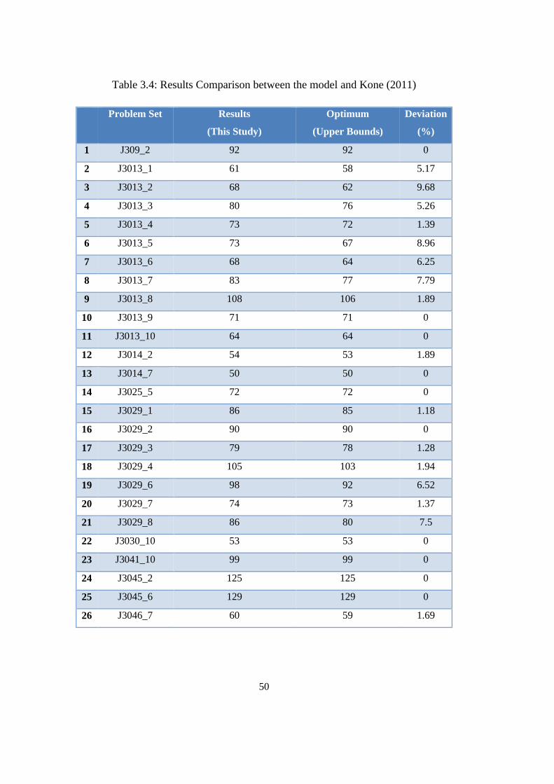
50
Table 3.4: Results Comparison between the model and Kone (2011)
Problem Set Results
(This Study)
Optimum
(Upper Bounds)
Deviation
(%)
1 J309_2 92 92 0
2 J3013_1 61 58 5.17
3 J3013_2 68 62 9.68
4 J3013_3 80 76 5.26
5 J3013_4 73 72 1.39
6 J3013_5 73 67 8.96
7 J3013_6 68 64 6.25
8 J3013_7 83 77 7.79
9 J3013_8 108 106 1.89
10 J3013_9 71 71 0
11 J3013_10 64 64 0
12 J3014_2 54 53 1.89
13 J3014_7 50 50 0
14 J3025_5 72 72 0
15 J3029_1 86 85 1.18
16 J3029_2 90 90 0
17 J3029_3 79 78 1.28
18 J3029_4 105 103 1.94
19 J3029_6 98 92 6.52
20 J3029_7 74 73 1.37
21 J3029_8 86 80 7.5
22 J3030_10 53 53 0
23 J3041_10 99 99 0
24 J3045_2 125 125 0
25 J3045_6 129 129 0
26 J3046_7 60 59 1.69
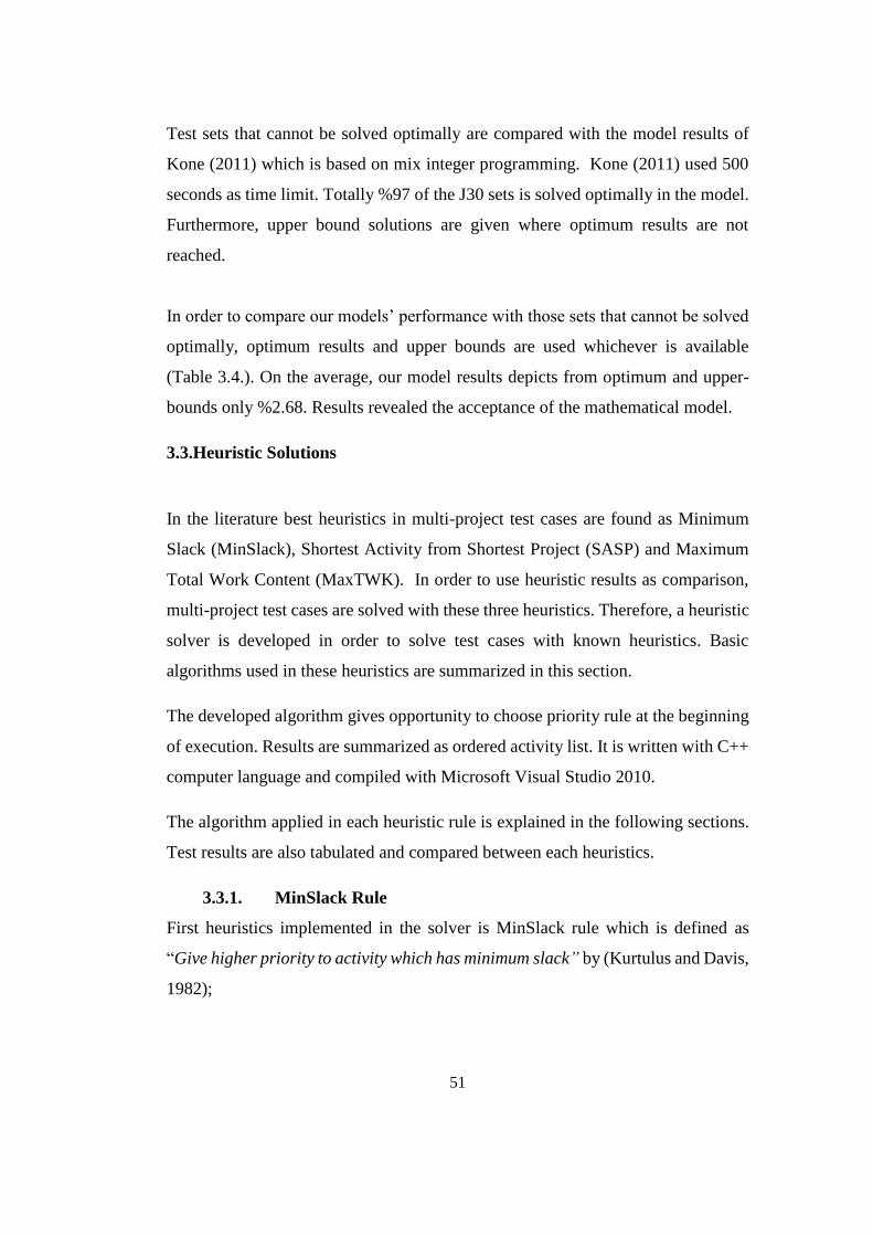
51
Test sets that cannot be solved optimally are compared with the model results of
Kone (2011) which is based on mix integer programming. Kone (2011) used 500
seconds as time limit. Totally %97 of the J30 sets is solved optimally in the model.
Furthermore, upper bound solutions are given where optimum results are not
reached.
In order to compare our models’ performance with those sets that cannot be solved
optimally, optimum results and upper bounds are used whichever is available
(Table 3.4.). On the average, our model results depicts from optimum and upper-
bounds only %2.68. Results revealed the acceptance of the mathematical model.
3.3.Heuristic Solutions
In the literature best heuristics in multi-project test cases are found as Minimum
Slack (MinSlack), Shortest Activity from Shortest Project (SASP) and Maximum
Total Work Content (MaxTWK). In order to use heuristic results as comparison,
multi-project test cases are solved with these three heuristics. Therefore, a heuristic
solver is developed in order to solve test cases with known heuristics. Basic
algorithms used in these heuristics are summarized in this section.
The developed algorithm gives opportunity to choose priority rule at the beginning
of execution. Results are summarized as ordered activity list. It is written with C++
computer language and compiled with Microsoft Visual Studio 2010.
The algorithm applied in each heuristic rule is explained in the following sections.
Test results are also tabulated and compared between each heuristics.
3.3.1. MinSlack Rule
First heuristics implemented in the solver is MinSlack rule which is defined as
“Give higher priority to activity which has minimum slack” by (Kurtulus and Davis,
1982);
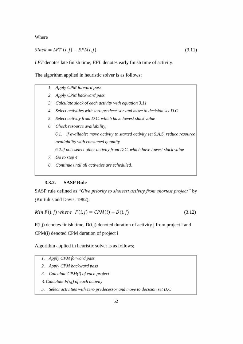
52
Where
𝑆𝑙𝑎𝑐𝑘 = 𝐿𝐹𝑇 (𝑖, 𝑗) − 𝐸𝐹𝐿(𝑖, 𝑗) (3.11)
LFT denotes late finish time; EFL denotes early finish time of activity.
The algorithm applied in heuristic solver is as follows;
1. Apply CPM forward pass
2. Apply CPM backward pass
3. Calculate slack of each activity with equation 3.11
4. Select activities with zero predecessor and move to decision set D.C
5. Select activity from D.C. which have lowest slack value
6. Check resource availability;
6.1. if available: move activity to started activity set S.A.S, reduce resource
availability with consumed quantity
6.2. if not: select other activity from D.C. which have lowest slack value
7. Go to step 4
8. Continue until all activities are scheduled.
3.3.2. SASP Rule
SASP rule defined as “Give priority to shortest activity from shortest project” by
(Kurtulus and Davis, 1982);
𝑀𝑖𝑛 𝐹(𝑖, 𝑗) 𝑤ℎ𝑒𝑟𝑒 𝐹(𝑖, 𝑗) = 𝐶𝑃𝑀(𝑖) − 𝐷(𝑖, 𝑗) (3.12)
F(i,j) denotes finish time, D(i,j) denoted duration of activity j from project i and
CPM(i) denoted CPM duration of project i
Algorithm applied in heuristic solver is as follows;
1. Apply CPM forward pass
2. Apply CPM backward pass
3. Calculate CPM(i) of each project
4. Calculate F(i,j) of each activity
5. Select activities with zero predecessor and move to decision set D.C
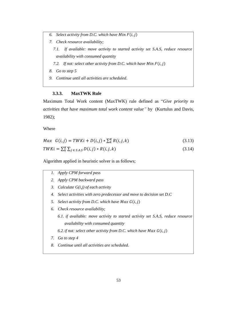
53
6. Select activity from D.C. which have 𝑀𝑖𝑛 𝐹(𝑖, 𝑗)
7. Check resource availability;
7.1. If available: move activity to started activity set S.A.S, reduce resource
availability with consumed quantity
7.2. If not: select other activity from D.C. which have 𝑀𝑖𝑛 𝐹(𝑖, 𝑗)
8. Go to step 5
9. Continue until all activities are scheduled.
3.3.3. MaxTWK Rule
Maximum Total Work content (MaxTWK) rule defined as “Give priority to
activities that have maximum total work content value” by (Kurtulus and Davis,
1982);
Where
𝑀𝑎𝑥 𝐺(𝑖, 𝑗) = 𝑇𝑊𝐾𝑖 + 𝐷(𝑖, 𝑗) ∗ ∑ 𝑅(𝑖, 𝑗, 𝑘)𝐾𝑘 (3.13)
𝑇𝑊𝐾𝑖 = ∑ ∑ 𝐷(𝑖, 𝑗) ∗ 𝑅(𝑖, 𝑗, 𝑘)𝑗 ∈ 𝑆.𝐴.𝑆𝐾𝑘 (3.14)
Algorithm applied in heuristic solver is as follows;
1. Apply CPM forward pass
2. Apply CPM backward pass
3. Calculate G(i,j) of each activity
4. Select activities with zero predecessor and move to decision set D.C
5. Select activity from D.C. which have 𝑀𝑎𝑥 𝐺(𝑖, 𝑗)
6. Check resource availability;
6.1. if available: move activity to started activity set S.A.S, reduce resource
availability with consumed quantity
6.2. if not: select other activity from D.C. which have 𝑀𝑎𝑥 𝐺(𝑖, 𝑗)
7. Go to step 4
8. Continue until all activities are scheduled.
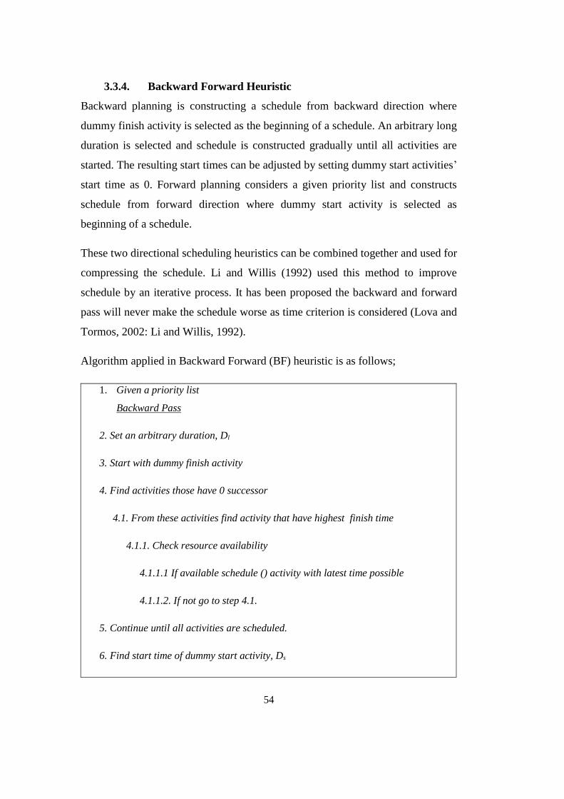
54
3.3.4. Backward Forward Heuristic
Backward planning is constructing a schedule from backward direction where
dummy finish activity is selected as the beginning of a schedule. An arbitrary long
duration is selected and schedule is constructed gradually until all activities are
started. The resulting start times can be adjusted by setting dummy start activities’
start time as 0. Forward planning considers a given priority list and constructs
schedule from forward direction where dummy start activity is selected as
beginning of a schedule.
These two directional scheduling heuristics can be combined together and used for
compressing the schedule. Li and Willis (1992) used this method to improve
schedule by an iterative process. It has been proposed the backward and forward
pass will never make the schedule worse as time criterion is considered (Lova and
Tormos, 2002: Li and Willis, 1992).
Algorithm applied in Backward Forward (BF) heuristic is as follows;
1. Given a priority list
Backward Pass
2. Set an arbitrary duration, Dl
3. Start with dummy finish activity
4. Find activities those have 0 successor
4.1. From these activities find activity that have highest finish time
4.1.1. Check resource availability
4.1.1.1 If available schedule () activity with latest time possible
4.1.1.2. If not go to step 4.1.
5. Continue until all activities are scheduled.
6. Find start time of dummy start activity, Ds
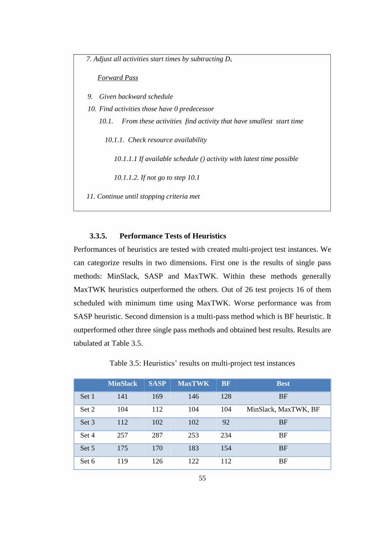
55
7. Adjust all activities start times by subtracting Ds
Forward Pass
9. Given backward schedule
10. Find activities those have 0 predecessor
10.1. From these activities find activity that have smallest start time
10.1.1. Check resource availability
10.1.1.1 If available schedule () activity with latest time possible
10.1.1.2. If not go to step 10.1
11. Continue until stopping criteria met
3.3.5. Performance Tests of Heuristics
Performances of heuristics are tested with created multi-project test instances. We
can categorize results in two dimensions. First one is the results of single pass
methods: MinSlack, SASP and MaxTWK. Within these methods generally
MaxTWK heuristics outperformed the others. Out of 26 test projects 16 of them
scheduled with minimum time using MaxTWK. Worse performance was from
SASP heuristic. Second dimension is a multi-pass method which is BF heuristic. It
outperformed other three single pass methods and obtained best results. Results are
tabulated at Table 3.5.
Table 3.5: Heuristics’ results on multi-project test instances
MinSlack SASP MaxTWK BF Best
Set 1 141 169 146 128 BF
Set 2 104 112 104 104 MinSlack, MaxTWK, BF
Set 3 112 102 102 92 BF
Set 4 257 287 253 234 BF
Set 5 175 170 183 154 BF
Set 6 119 126 122 112 BF
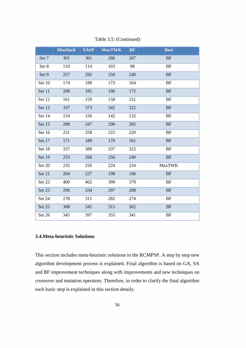
56
MinSlack SASP MaxTWK BF Best
Set 7 301 301 286 267 BF
Set 8 110 114 103 98 BF
Set 9 257 292 250 240 BF
Set 10 174 188 173 164 BF
Set 11 208 185 196 172 BF
Set 12 161 159 158 151 BF
Set 13 337 373 342 322 BF
Set 14 154 156 142 132 BF
Set 15 288 347 290 285 BF
Set 16 231 258 225 220 BF
Set 17 171 189 170 161 BF
Set 18 337 389 337 322 BF
Set 19 253 268 256 240 BF
Set 20 235 256 224 234 MaxTWK
Set 21 204 227 198 196 BF
Set 22 400 462 399 379 BF
Set 23 296 334 297 288 BF
Set 24 278 311 282 274 BF
Set 25 308 345 315 302 BF
Set 26 345 397 355 341 BF
3.4.Meta-heuristic Solutions
This section includes meta-heuristic solutions to the RCMPSP. A step by step new
algorithm development process is explained. Final algorithm is based on GA, SA
and BF improvement techniques along with improvements and new techniques on
crossover and mutation operators. Therefore, in order to clarify the final algorithm
each basic step is explained in this section detaily.
Table 3.5: (Continued)
57
3.4.1. A Sole GA
Algorithm development process within the meta-heuristic solutions was started
with a sole GA. To start with a GA, one has to decide the method of GA which
consists of its chromosome coding and decoding, fitness evaluation procedure,
crossover, mutation and selection. Before proceeding to details of the algorithm
mechanism is explained as follows;
1. Encode schedule into random key based chromosomes
2. Define fitness function
3. Define elitism, crossover and mutation ratio
4. Generate random initial population of chromosomes
5. Set current population
5.1. Generate new solutions via crossover and mutation
5.1.1. If better accept new solutions
5.1.2. If not reject
5.2. Select better chromosomes via selection mechanism and copy them to new
population
5.3. Protect %5 of chromosomes and copy them to new population
5.4. Replace current population with new population
6. Continue until stopping criteria met and go to step 5
3.4.1.1.Chromosome Coding and Decoding
Each chromosome consists ∑ 𝑁(𝑖)𝑀𝑖=1 number of genes where each gene represents
the priority number of an activity. Starting from dummy start activity to dummy
finish activity each gene has a value between 0 and 1. First N1 genes represent
activities from project 1, second N2 genes represent activities from project 2 and it
continues to number of project M. General representation can be seen from Figure
3.1.
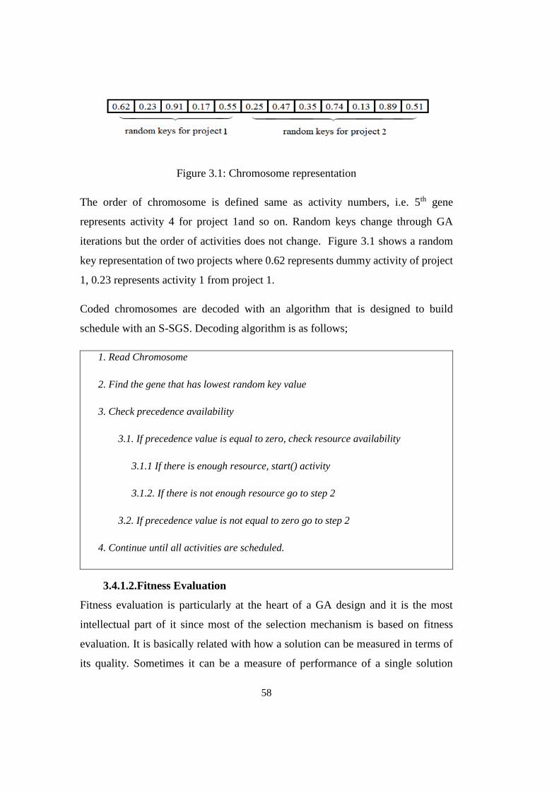
58
Figure 3.1: Chromosome representation
The order of chromosome is defined same as activity numbers, i.e. 5th gene
represents activity 4 for project 1and so on. Random keys change through GA
iterations but the order of activities does not change. Figure 3.1 shows a random
key representation of two projects where 0.62 represents dummy activity of project
1, 0.23 represents activity 1 from project 1.
Coded chromosomes are decoded with an algorithm that is designed to build
schedule with an S-SGS. Decoding algorithm is as follows;
1. Read Chromosome
2. Find the gene that has lowest random key value
3. Check precedence availability
3.1. If precedence value is equal to zero, check resource availability
3.1.1 If there is enough resource, start() activity
3.1.2. If there is not enough resource go to step 2
3.2. If precedence value is not equal to zero go to step 2
4. Continue until all activities are scheduled.
3.4.1.2.Fitness Evaluation
Fitness evaluation is particularly at the heart of a GA design and it is the most
intellectual part of it since most of the selection mechanism is based on fitness
evaluation. It is basically related with how a solution can be measured in terms of
its quality. Sometimes it can be a measure of performance of a single solution
59
output. Therefore, fitness function used in this GA is selected as the total duration
of project portfolio.
Fitness Function:
𝐶𝑚𝑎𝑥 (3.15)
Fitness calculation algorithm is as follows:
1. Read activity ordered list
2. Start activity with earliest time possible
3. Read last activity’s finish time
3.4.1.3.Crossover
One point crossover is applied to chromosomes where crossover ratio is predefined
before the algorithm is started.
Algorithm designed for crossover is as follows;
1. Read crossover ratio
2. Select father and mother chromosome randomly from population
3. Randomly generate a number r between 1 and N, where N is the total activity
number
4. Change genes from 1 to r and r+1 to N between father and mother chromosomes
5. Continue until crossover ratio is reached.
3.4.1.4.Mutation
Mutation is necessary in any GA in order to prevent premature convergence of the
algorithm. Therefore, a standard mutation technique is applied. In this technique,
randomly selected genes are applied to change its random key value.
Algorithm designed for mutation is as follows;
60
1. Read mutation ratio
2. Randomly select chromosomes where mutation is applied.
2.1. Randomly select genes on this chromosome
2.1.1. Replace its value by a new random key number
3. Continue until mutation ratio is reached.
3.4.1.5.Roulette Wheel Selection
The idea of evolutionary computing is to give higher change to better chromosomes.
Therefore as population evolves better chromosomes should have higher chance to
live. In order to apply this principle, some kind of selection methods should be used.
In this simple GA roulette wheel selection method is used through iterations. In this
method, those schedules which are shorter have high probability of selection.
Probability of a chromosome selected calculated as:
1
𝑃(𝑖) 𝑤ℎ𝑒𝑟𝑒 𝑃(𝑖) =
𝐹𝑖𝑡𝑛𝑒𝑠𝑠 (𝑖)∑ 𝐹𝑖𝑡𝑛𝑒𝑠𝑠(𝑗)𝑁
𝐽=1⁄ (3.16)
As the equation implies if a solution have good fitness values, its probability value
would be higher so that probability of selected would be higher.
Algorithm designed for roulette wheel selection is as follows;
1. Find all fitness values of a population,
2. Calculate P(i) of each chromosome,
3. Sort all chromosomes in ascending form according to P(i) values where
0≤P(i)≤1
4. Create a random number where 0≤ r ≤1
5. Select chromosome that corresponds random number r
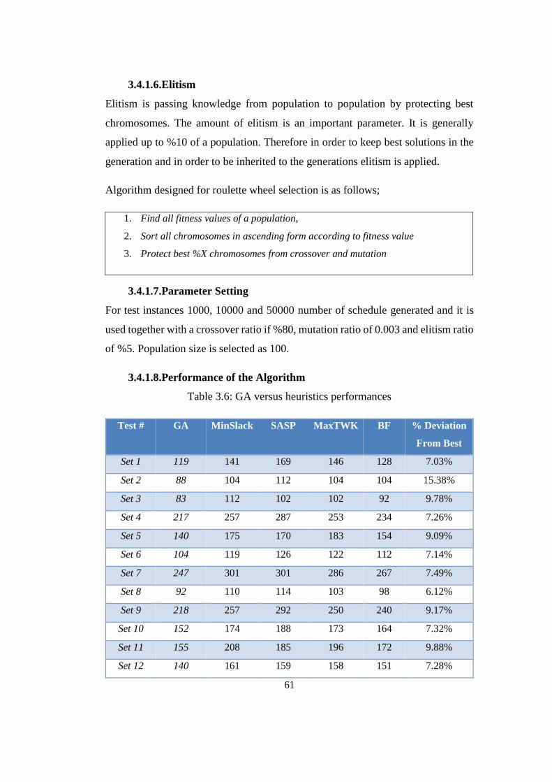
61
3.4.1.6.Elitism
Elitism is passing knowledge from population to population by protecting best
chromosomes. The amount of elitism is an important parameter. It is generally
applied up to %10 of a population. Therefore in order to keep best solutions in the
generation and in order to be inherited to the generations elitism is applied.
Algorithm designed for roulette wheel selection is as follows;
1. Find all fitness values of a population,
2. Sort all chromosomes in ascending form according to fitness value
3. Protect best %X chromosomes from crossover and mutation
3.4.1.7.Parameter Setting
For test instances 1000, 10000 and 50000 number of schedule generated and it is
used together with a crossover ratio if %80, mutation ratio of 0.003 and elitism ratio
of %5. Population size is selected as 100.
3.4.1.8.Performance of the Algorithm
Table 3.6: GA versus heuristics performances
Test # GA MinSlack SASP MaxTWK BF % Deviation
From Best
Set 1 119 141 169 146 128 7.03%
Set 2 88 104 112 104 104 15.38%
Set 3 83 112 102 102 92 9.78%
Set 4 217 257 287 253 234 7.26%
Set 5 140 175 170 183 154 9.09%
Set 6 104 119 126 122 112 7.14%
Set 7 247 301 301 286 267 7.49%
Set 8 92 110 114 103 98 6.12%
Set 9 218 257 292 250 240 9.17%
Set 10 152 174 188 173 164 7.32%
Set 11 155 208 185 196 172 9.88%
Set 12 140 161 159 158 151 7.28%
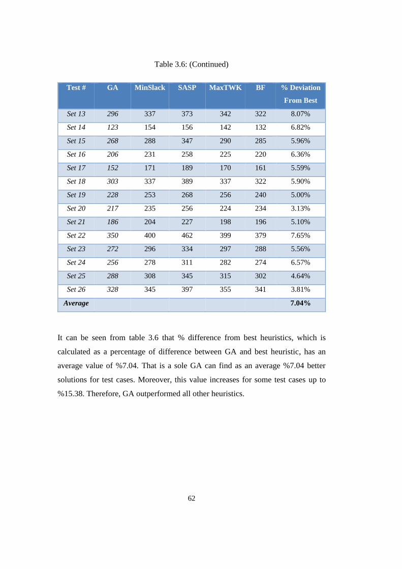
62
Test # GA MinSlack SASP MaxTWK BF % Deviation
From Best
Set 13 296 337 373 342 322 8.07%
Set 14 123 154 156 142 132 6.82%
Set 15 268 288 347 290 285 5.96%
Set 16 206 231 258 225 220 6.36%
Set 17 152 171 189 170 161 5.59%
Set 18 303 337 389 337 322 5.90%
Set 19 228 253 268 256 240 5.00%
Set 20 217 235 256 224 234 3.13%
Set 21 186 204 227 198 196 5.10%
Set 22 350 400 462 399 379 7.65%
Set 23 272 296 334 297 288 5.56%
Set 24 256 278 311 282 274 6.57%
Set 25 288 308 345 315 302 4.64%
Set 26 328 345 397 355 341 3.81%
Average 7.04%
It can be seen from table 3.6 that % difference from best heuristics, which is
calculated as a percentage of difference between GA and best heuristic, has an
average value of %7.04. That is a sole GA can find as an average %7.04 better
solutions for test cases. Moreover, this value increases for some test cases up to
%15.38. Therefore, GA outperformed all other heuristics.
Table 3.6: (Continued)
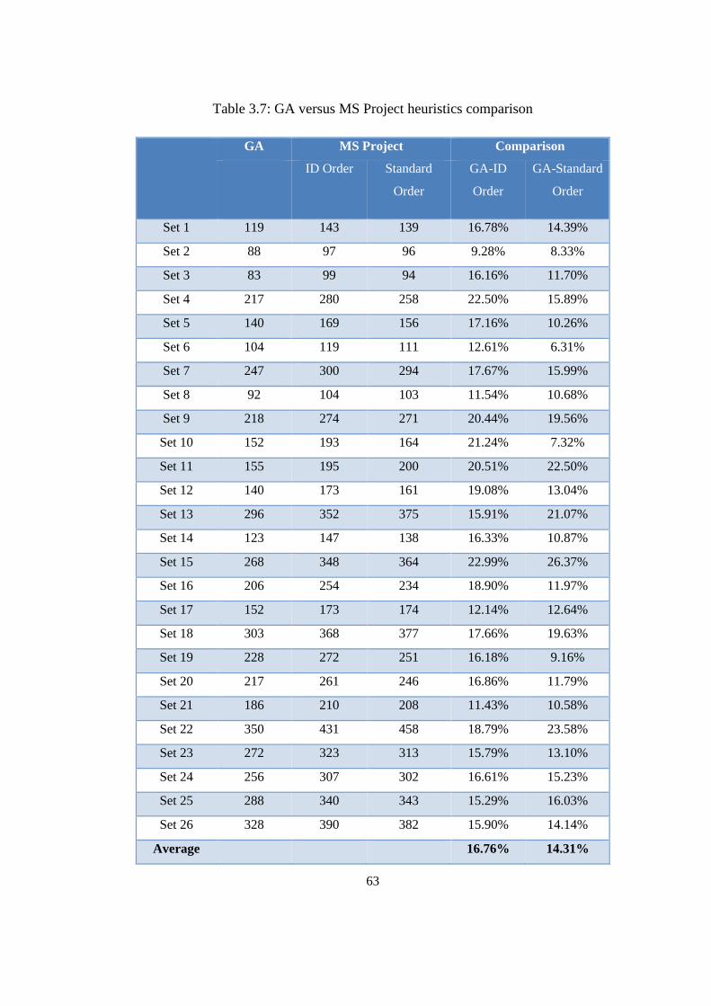
63
Table 3.7: GA versus MS Project heuristics comparison
GA MS Project Comparison
ID Order Standard
Order
GA-ID
Order
GA-Standard
Order
Set 1 119 143 139 16.78% 14.39%
Set 2 88 97 96 9.28% 8.33%
Set 3 83 99 94 16.16% 11.70%
Set 4 217 280 258 22.50% 15.89%
Set 5 140 169 156 17.16% 10.26%
Set 6 104 119 111 12.61% 6.31%
Set 7 247 300 294 17.67% 15.99%
Set 8 92 104 103 11.54% 10.68%
Set 9 218 274 271 20.44% 19.56%
Set 10 152 193 164 21.24% 7.32%
Set 11 155 195 200 20.51% 22.50%
Set 12 140 173 161 19.08% 13.04%
Set 13 296 352 375 15.91% 21.07%
Set 14 123 147 138 16.33% 10.87%
Set 15 268 348 364 22.99% 26.37%
Set 16 206 254 234 18.90% 11.97%
Set 17 152 173 174 12.14% 12.64%
Set 18 303 368 377 17.66% 19.63%
Set 19 228 272 251 16.18% 9.16%
Set 20 217 261 246 16.86% 11.79%
Set 21 186 210 208 11.43% 10.58%
Set 22 350 431 458 18.79% 23.58%
Set 23 272 323 313 15.79% 13.10%
Set 24 256 307 302 16.61% 15.23%
Set 25 288 340 343 15.29% 16.03%
Set 26 328 390 382 15.90% 14.14%
Average 16.76% 14.31%
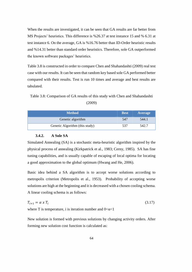
64
When the results are investigated, it can be seen that GA results are far better from
MS Projects’ heuristics. This difference is %26.37 at test instance 15 and % 6.31 at
test instance 6. On the average, GA is %16.76 better than ID-Order heuristic results
and %14.31 better than standard order heuristics. Therefore, sole GA outperformed
the known software packages’ heuristics.
Table 3.8 is constructed in order to compare Chen and Shahandashti (2009) real test
case with our results. It can be seen that random key based sole GA performed better
compared with their results. Test is run 10 times and average and best results are
tabulated.
Table 3.8: Comparison of GA results of this study with Chen and Shahandashti
(2009)
Method Best Average
Genetic algorithm 547 544.1
Genetic Algorithm (this study) 537 542.7
3.4.2. A Sole SA
Simulated Annealing (SA) is a stochastic meta-heuristic algorithm inspired by the
physical process of annealing (Kirkpatrick et al., 1983; Cerny, 1985). SA has fine
tuning capabilities, and is usually capable of escaping of local optima for locating
a good approximation to the global optimum (Hwang and He, 2006).
Basic idea behind a SA algorithm is to accept worse solutions according to
metropolis criterion (Metropolis et al., 1953). Probability of accepting worse
solutions are high at the beginning and it is decreased with a chosen cooling schema.
A linear cooling schema is as follows:
𝑇𝑖+1 = 𝛼 𝑥 𝑇𝑖 (3.17)
where T is temperature, i is iteration number and 0<α<1
New solution is formed with previous solutions by changing activity orders. After
forming new solution cost function is calculated as:
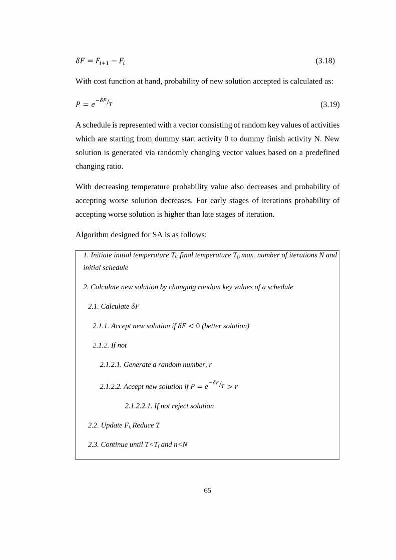
65
𝛿𝐹 = 𝐹𝑖+1 − 𝐹𝑖 (3.18)
With cost function at hand, probability of new solution accepted is calculated as:
𝑃 = 𝑒−𝛿𝐹
𝑇⁄ (3.19)
A schedule is represented with a vector consisting of random key values of activities
which are starting from dummy start activity 0 to dummy finish activity N. New
solution is generated via randomly changing vector values based on a predefined
changing ratio.
With decreasing temperature probability value also decreases and probability of
accepting worse solution decreases. For early stages of iterations probability of
accepting worse solution is higher than late stages of iteration.
Algorithm designed for SA is as follows:
1. Initiate initial temperature T0 ,final temperature Tf, max. number of iterations N and
initial schedule
2. Calculate new solution by changing random key values of a schedule
2.1. Calculate 𝛿𝐹
2.1.1. Accept new solution if 𝛿𝐹 < 0 (better solution)
2.1.2. If not
2.1.2.1. Generate a random number, r
2.1.2.2. Accept new solution if 𝑃 = 𝑒−𝛿𝐹
𝑇⁄ > 𝑟
2.1.2.2.1. If not reject solution
2.2. Update Fi, Reduce T
2.3. Continue until T<Tf and n<N
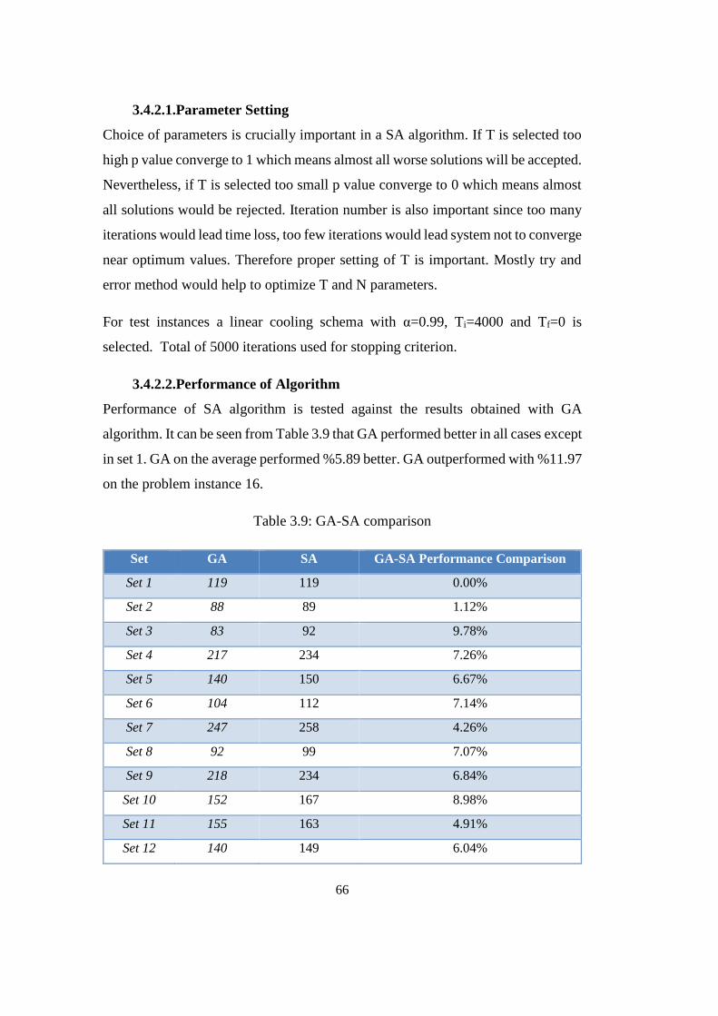
66
3.4.2.1.Parameter Setting
Choice of parameters is crucially important in a SA algorithm. If T is selected too
high p value converge to 1 which means almost all worse solutions will be accepted.
Nevertheless, if T is selected too small p value converge to 0 which means almost
all solutions would be rejected. Iteration number is also important since too many
iterations would lead time loss, too few iterations would lead system not to converge
near optimum values. Therefore proper setting of T is important. Mostly try and
error method would help to optimize T and N parameters.
For test instances a linear cooling schema with α=0.99, Ti=4000 and Tf=0 is
selected. Total of 5000 iterations used for stopping criterion.
3.4.2.2.Performance of Algorithm
Performance of SA algorithm is tested against the results obtained with GA
algorithm. It can be seen from Table 3.9 that GA performed better in all cases except
in set 1. GA on the average performed %5.89 better. GA outperformed with %11.97
on the problem instance 16.
Table 3.9: GA-SA comparison
Set GA SA GA-SA Performance Comparison
Set 1 119 119 0.00%
Set 2 88 89 1.12%
Set 3 83 92 9.78%
Set 4 217 234 7.26%
Set 5 140 150 6.67%
Set 6 104 112 7.14%
Set 7 247 258 4.26%
Set 8 92 99 7.07%
Set 9 218 234 6.84%
Set 10 152 167 8.98%
Set 11 155 163 4.91%
Set 12 140 149 6.04%
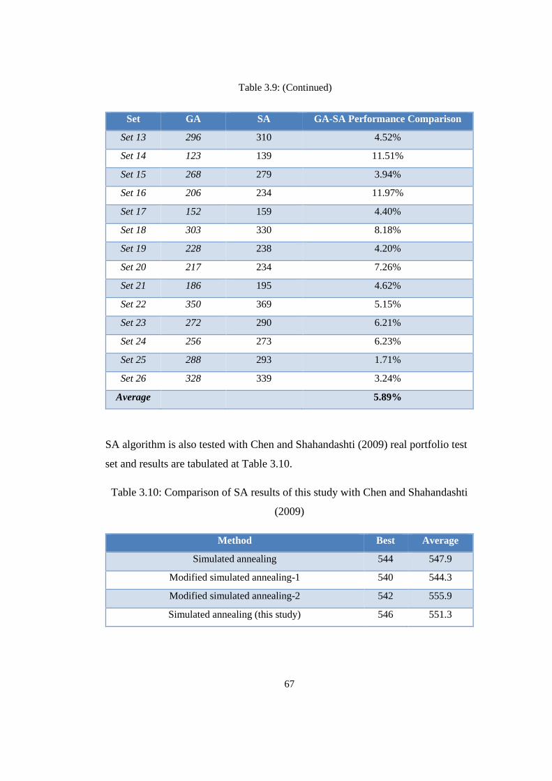
67
Set GA SA GA-SA Performance Comparison
Set 13 296 310 4.52%
Set 14 123 139 11.51%
Set 15 268 279 3.94%
Set 16 206 234 11.97%
Set 17 152 159 4.40%
Set 18 303 330 8.18%
Set 19 228 238 4.20%
Set 20 217 234 7.26%
Set 21 186 195 4.62%
Set 22 350 369 5.15%
Set 23 272 290 6.21%
Set 24 256 273 6.23%
Set 25 288 293 1.71%
Set 26 328 339 3.24%
Average 5.89%
SA algorithm is also tested with Chen and Shahandashti (2009) real portfolio test
set and results are tabulated at Table 3.10.
Table 3.10: Comparison of SA results of this study with Chen and Shahandashti
(2009)
Method Best Average
Simulated annealing 544 547.9
Modified simulated annealing-1 540 544.3
Modified simulated annealing-2 542 555.9
Simulated annealing (this study) 546 551.3
Table 3.9: (Continued)
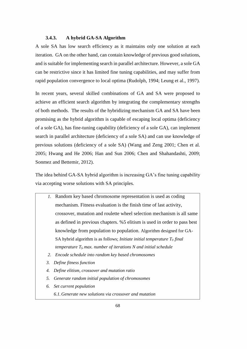
68
3.4.3. A hybrid GA-SA Algorithm
A sole SA has low search efficiency as it maintains only one solution at each
iteration. GA on the other hand, can contain knowledge of previous good solutions,
and is suitable for implementing search in parallel architecture. However, a sole GA
can be restrictive since it has limited fine tuning capabilities, and may suffer from
rapid population convergence to local optima (Rudolph, 1994; Leung et al., 1997).
In recent years, several skilled combinations of GA and SA were proposed to
achieve an efficient search algorithm by integrating the complementary strengths
of both methods. The results of the hybridizing mechanism GA and SA have been
promising as the hybrid algorithm is capable of escaping local optima (deficiency
of a sole GA), has fine-tuning capability (deficiency of a sole GA), can implement
search in parallel architecture (deficiency of a sole SA) and can use knowledge of
previous solutions (deficiency of a sole SA) (Wang and Zeng 2001; Chen et al.
2005; Hwang and He 2006; Han and Sun 2006; Chen and Shahandashti, 2009;
Sonmez and Bettemir, 2012).
The idea behind GA-SA hybrid algorithm is increasing GA’s fine tuning capability
via accepting worse solutions with SA principles.
1. Random key based chromosome representation is used as coding
mechanism. Fitness evaluation is the finish time of last activity,
crossover, mutation and roulette wheel selection mechanism is all same
as defined in previous chapters. %5 elitism is used in order to pass best
knowledge from population to population. Algorithm designed for GA-
SA hybrid algorithm is as follows; Initiate initial temperature T0 ,final
temperature Tf, max. number of iterations N and initial schedule
2. Encode schedule into random key based chromosomes
3. Define fitness function
4. Define elitism, crossover and mutation ratio
5. Generate random initial population of chromosomes
6. Set current population
6.1. Generate new solutions via crossover and mutation
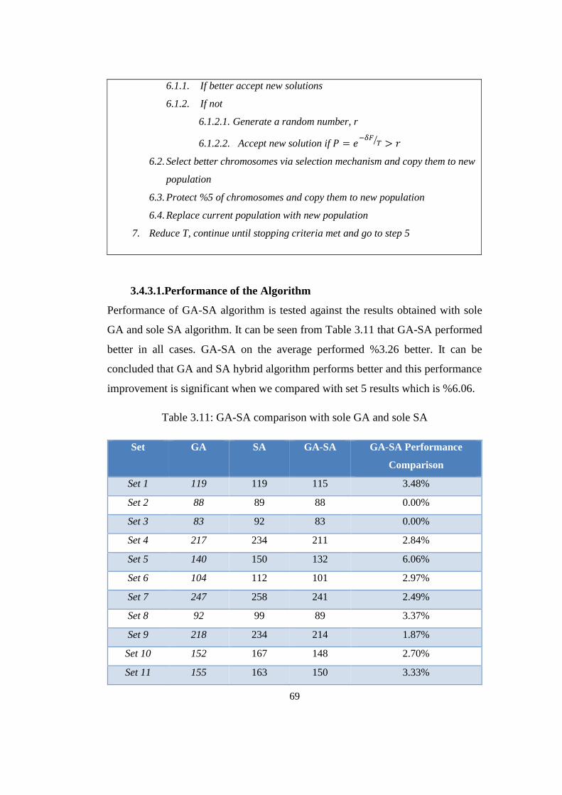
69
6.1.1. If better accept new solutions
6.1.2. If not
6.1.2.1. Generate a random number, r
6.1.2.2. Accept new solution if 𝑃 = 𝑒−𝛿𝐹
𝑇⁄ > 𝑟
6.2. Select better chromosomes via selection mechanism and copy them to new
population
6.3. Protect %5 of chromosomes and copy them to new population
6.4. Replace current population with new population
7. Reduce T, continue until stopping criteria met and go to step 5
3.4.3.1.Performance of the Algorithm
Performance of GA-SA algorithm is tested against the results obtained with sole
GA and sole SA algorithm. It can be seen from Table 3.11 that GA-SA performed
better in all cases. GA-SA on the average performed %3.26 better. It can be
concluded that GA and SA hybrid algorithm performs better and this performance
improvement is significant when we compared with set 5 results which is %6.06.
Table 3.11: GA-SA comparison with sole GA and sole SA
Set GA SA GA-SA GA-SA Performance
Comparison
Set 1 119 119 115 3.48%
Set 2 88 89 88 0.00%
Set 3 83 92 83 0.00%
Set 4 217 234 211 2.84%
Set 5 140 150 132 6.06%
Set 6 104 112 101 2.97%
Set 7 247 258 241 2.49%
Set 8 92 99 89 3.37%
Set 9 218 234 214 1.87%
Set 10 152 167 148 2.70%
Set 11 155 163 150 3.33%
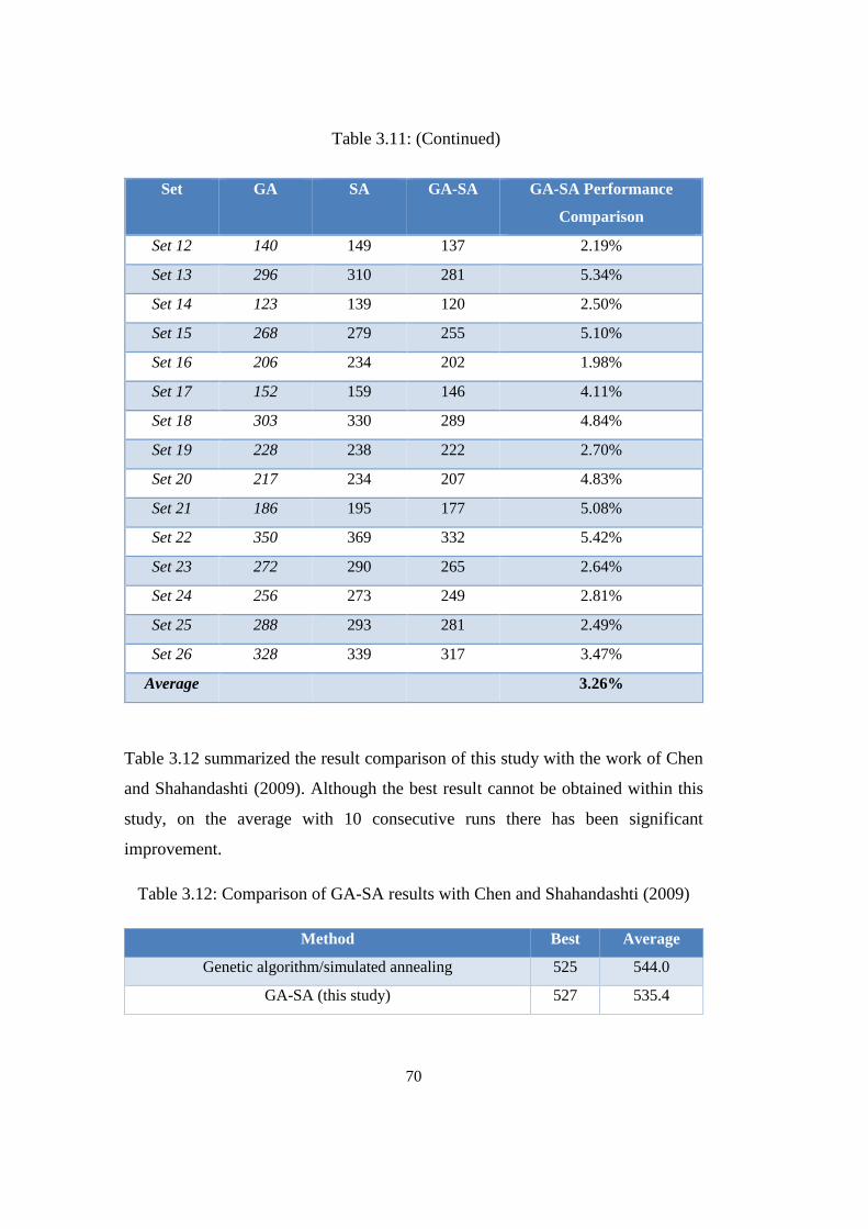
70
Set GA SA GA-SA GA-SA Performance
Comparison
Set 12 140 149 137 2.19%
Set 13 296 310 281 5.34%
Set 14 123 139 120 2.50%
Set 15 268 279 255 5.10%
Set 16 206 234 202 1.98%
Set 17 152 159 146 4.11%
Set 18 303 330 289 4.84%
Set 19 228 238 222 2.70%
Set 20 217 234 207 4.83%
Set 21 186 195 177 5.08%
Set 22 350 369 332 5.42%
Set 23 272 290 265 2.64%
Set 24 256 273 249 2.81%
Set 25 288 293 281 2.49%
Set 26 328 339 317 3.47%
Average 3.26%
Table 3.12 summarized the result comparison of this study with the work of Chen
and Shahandashti (2009). Although the best result cannot be obtained within this
study, on the average with 10 consecutive runs there has been significant
improvement.
Table 3.12: Comparison of GA-SA results with Chen and Shahandashti (2009)
Method Best Average
Genetic algorithm/simulated annealing 525 544.0
GA-SA (this study) 527 535.4
Table 3.11: (Continued)
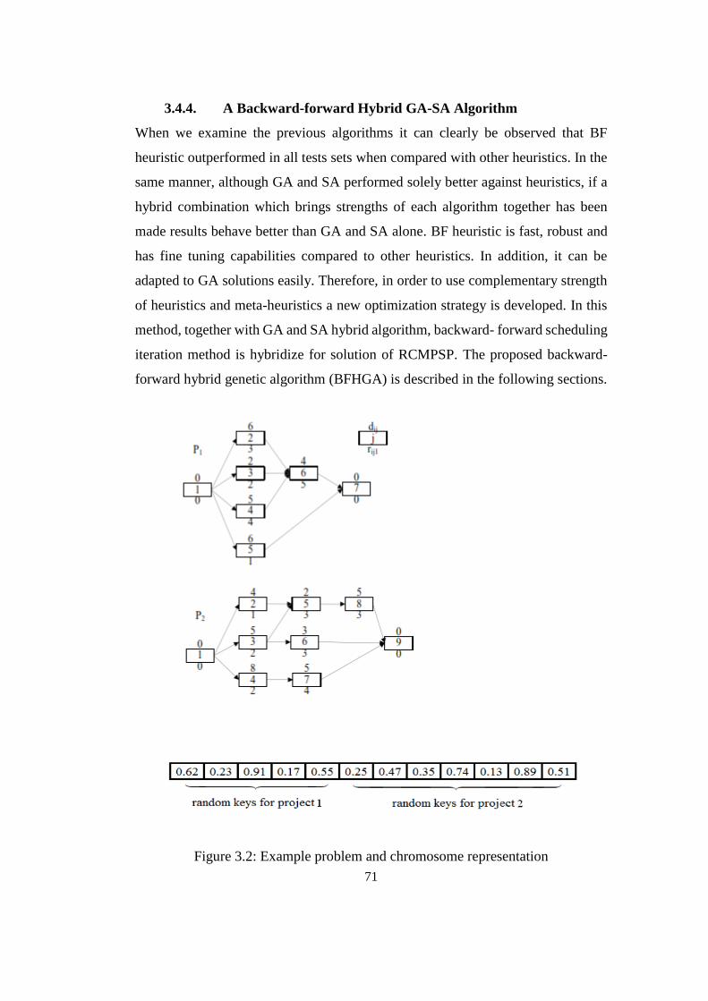
71
3.4.4. A Backward-forward Hybrid GA-SA Algorithm
When we examine the previous algorithms it can clearly be observed that BF
heuristic outperformed in all tests sets when compared with other heuristics. In the
same manner, although GA and SA performed solely better against heuristics, if a
hybrid combination which brings strengths of each algorithm together has been
made results behave better than GA and SA alone. BF heuristic is fast, robust and
has fine tuning capabilities compared to other heuristics. In addition, it can be
adapted to GA solutions easily. Therefore, in order to use complementary strength
of heuristics and meta-heuristics a new optimization strategy is developed. In this
method, together with GA and SA hybrid algorithm, backward- forward scheduling
iteration method is hybridize for solution of RCMPSP. The proposed backward-
forward hybrid genetic algorithm (BFHGA) is described in the following sections.
Figure 3.2: Example problem and chromosome representation
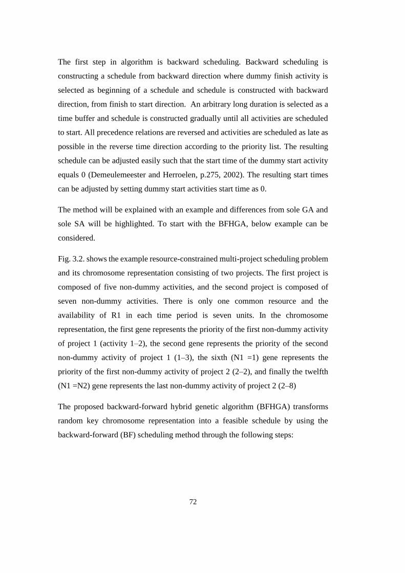
72
The first step in algorithm is backward scheduling. Backward scheduling is
constructing a schedule from backward direction where dummy finish activity is
selected as beginning of a schedule and schedule is constructed with backward
direction, from finish to start direction. An arbitrary long duration is selected as a
time buffer and schedule is constructed gradually until all activities are scheduled
to start. All precedence relations are reversed and activities are scheduled as late as
possible in the reverse time direction according to the priority list. The resulting
schedule can be adjusted easily such that the start time of the dummy start activity
equals 0 (Demeulemeester and Herroelen, p.275, 2002). The resulting start times
can be adjusted by setting dummy start activities start time as 0.
The method will be explained with an example and differences from sole GA and
sole SA will be highlighted. To start with the BFHGA, below example can be
considered.
Fig. 3.2. shows the example resource-constrained multi-project scheduling problem
and its chromosome representation consisting of two projects. The first project is
composed of five non-dummy activities, and the second project is composed of
seven non-dummy activities. There is only one common resource and the
availability of R1 in each time period is seven units. In the chromosome
representation, the first gene represents the priority of the first non-dummy activity
of project 1 (activity 1–2), the second gene represents the priority of the second
non-dummy activity of project 1 (1–3), the sixth (N1 =1) gene represents the
priority of the first non-dummy activity of project 2 (2–2), and finally the twelfth
(N1 =N2) gene represents the last non-dummy activity of project 2 (2–8)
The proposed backward-forward hybrid genetic algorithm (BFHGA) transforms
random key chromosome representation into a feasible schedule by using the
backward-forward (BF) scheduling method through the following steps:
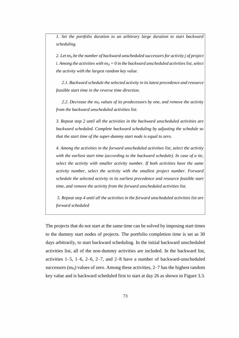
73
1. Set the portfolio duration to an arbitrary large duration to start backward
scheduling.
2. Let nsij be the number of backward-unscheduled successors for activity j of project
i. Among the activities with nsij = 0 in the backward unscheduled activities list, select
the activity with the largest random key value.
2.1. Backward schedule the selected activity in its latest precedence and resource
feasible start time in the reverse time direction.
2.2. Decrease the nsij values of its predecessors by one, and remove the activity
from the backward unscheduled activities list.
3. Repeat step 2 until all the activities in the backward unscheduled activities are
backward scheduled. Complete backward scheduling by adjusting the schedule so
that the start time of the super-dummy start node is equal to zero.
4. Among the activities in the forward unscheduled activities list, select the activity
with the earliest start time (according to the backward schedule). In case of a tie,
select the activity with smaller activity number. If both activities have the same
activity number, select the activity with the smallest project number. Forward
schedule the selected activity in its earliest precedence and resource feasible start
time, and remove the activity from the forward unscheduled activities list.
5. Repeat step 4 until all the activities in the forward unscheduled activities list are
forward scheduled
The projects that do not start at the same time can be solved by imposing start times
to the dummy start nodes of projects. The portfolio completion time is set as 30
days arbitrarily, to start backward scheduling. In the initial backward unscheduled
activities list, all of the non-dummy activities are included. In the backward list,
activities 1–5, 1–6, 2–6, 2–7, and 2–8 have a number of backward-unscheduled
successors (nsij) values of zero. Among these activities, 2–7 has the highest random
key value and is backward scheduled first to start at day 26 as shown in Figure 3.3.
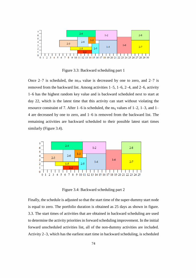
74
Figure 3.3: Backward scheduling part 1
Once 2–7 is scheduled, the ns24 value is decreased by one to zero, and 2–7 is
removed from the backward list. Among activities 1–5, 1–6, 2–4, and 2–6, activity
1–6 has the highest random key value and is backward scheduled next to start at
day 22, which is the latest time that this activity can start without violating the
resource constraint of 7. After 1–6 is scheduled, the nsij values of 1–2, 1–3, and 1–
4 are decreased by one to zero, and 1–6 is removed from the backward list. The
remaining activities are backward scheduled to their possible latest start times
similarly (Figure 3.4).
Figure 3.4: Backward scheduling part 2
Finally, the schedule is adjusted so that the start time of the super-dummy start node
is equal to zero. The portfolio duration is obtained as 25 days as shown in figure.
3.3. The start times of activities that are obtained in backward scheduling are used
to determine the activity priorities in forward scheduling improvement. In the initial
forward unscheduled activities list, all of the non-dummy activities are included.
Activity 2–3, which has the earliest start time in backward scheduling, is scheduled
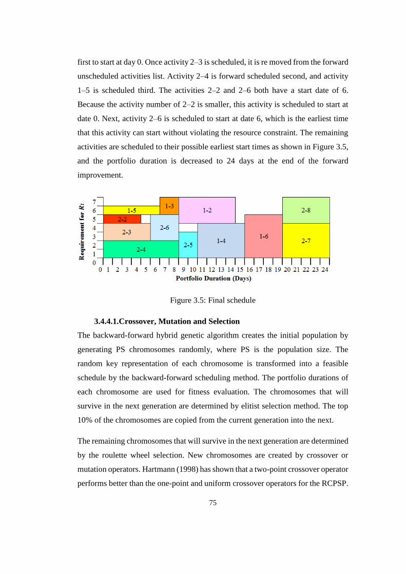
75
first to start at day 0. Once activity 2–3 is scheduled, it is re moved from the forward
unscheduled activities list. Activity 2–4 is forward scheduled second, and activity
1–5 is scheduled third. The activities 2–2 and 2–6 both have a start date of 6.
Because the activity number of 2–2 is smaller, this activity is scheduled to start at
date 0. Next, activity 2–6 is scheduled to start at date 6, which is the earliest time
that this activity can start without violating the resource constraint. The remaining
activities are scheduled to their possible earliest start times as shown in Figure 3.5,
and the portfolio duration is decreased to 24 days at the end of the forward
improvement.
Figure 3.5: Final schedule
3.4.4.1.Crossover, Mutation and Selection
The backward-forward hybrid genetic algorithm creates the initial population by
generating PS chromosomes randomly, where PS is the population size. The
random key representation of each chromosome is transformed into a feasible
schedule by the backward-forward scheduling method. The portfolio durations of
each chromosome are used for fitness evaluation. The chromosomes that will
survive in the next generation are determined by elitist selection method. The top
10% of the chromosomes are copied from the current generation into the next.
The remaining chromosomes that will survive in the next generation are determined
by the roulette wheel selection. New chromosomes are created by crossover or
mutation operators. Hartmann (1998) has shown that a two-point crossover operator
performs better than the one-point and uniform crossover operators for the RCPSP.
76
Hence, in BFHGA, two chromosomes are combined by using a two-point crossover
operator. Mutation is performed by changing a number of random keys of selected
chromosomes with new random keys.
3.4.4.2.Integration of Simulated Annealing
The SA is integrated into GA during mutation in the proposed hybrid algorithm. In
BFHGA, two types of mutations are performed. The first type of mutation is
performed after a crossover operation when there is not sufficient diversification
between a child and one of its parents. The elitist selection method adopted in
BFHGA can lead to a homogeneous population that may result in rapid population
convergence to a local optimum. Hence, the first type of mutation is performed on
a child after the crossover operation, when the mean absolute difference of random
key values of a child and one of its parents (father or mother) is smaller than a
predefined diversification value τ (Equation 3.19). The value of τ is reduced based
on a cooling scheme defined by temperature t.
Do Mutation
While ∑ |𝑅𝐾𝑐ℎ𝑖𝑙𝑑 − 𝑅𝐾𝑝𝑎𝑟𝑒𝑛𝑡𝑠|𝑁𝑖=0
𝑁⁄ ≤ τ (3.19)
The second type of mutation is the regular mutation that is performed randomly
based on a predefined mutation rate. The main objective of both types of mutations
is to achieve diversification for escaping premature convergence to achieve the
global optimum or near-global optimum results.
In BFHGA, every mutation that leads to a chromosome with a better (or equal)
fitness evaluation function value is accepted. However, a mutation that leads to a
chromosome with a worse fitness evaluation function value may be accepted or
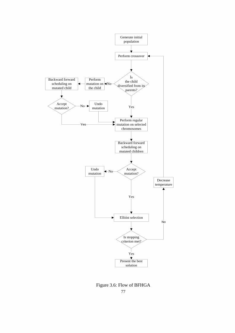
77
Generate initial
population
Perform crossover
İs
the child
diversified from its
parents?
Perform
mutation on
the child
No
Perform regular
mutation on selected
chromosomes
YesAccept
mutation?
Undo
mutationNo
Yes
Accept
mutation?
Yes
Undo
mutationNo
Is stopping
criterion met?
Yes
Present the best
solution
No
Decrease
temperature
Backward forward
scheduling on
mutated child
Backward forward
scheduling on
mutated children
Ellitist selection
Figure 3.6: Flow of BFHGA
78
rejected (not executed) based on a decision function (DF1). The general flow of
BFHGA can be seen at Figure 3.6 and the decision function DF1 is defined in
Equation (3.20) as follows:
t
Bx
sf
'fsfs
u
t
Bx
sf
"fsfs
u
erifreject
erifaccept
1DF (3.20)
3.4.4.3.Performance of Algorithm
The initial comparisons include four single project RCPSP case examples. The
sources of the examples were Anagnostopoulos and Koulinas (2012),
Christodoulou (2010), Hegazy (1999), and Leu and Yang (1999) respectively. The
single project examples included between 17 and 25 activities, and one and six
resources. The optimal solutions for the first three case examples were obtained by
using RESCON (Deblaere et. al. 2011). RESCON can obtain the optimal solutions
for relatively small resource constrained project networks including finish to start
precedence relations. The fourth single project case example was not solved by
RESCON, since this example included start-to-start type of precedence relations.
As can be summarized at Table 3.13, the BFHGA algorithm was able to obtain the
optimal solutions of 54, 133, and 43 days for single-project case examples one, two,
and three, respectively. The algorithm also successfully determined the best
available solution (upper bound) 35 days for case example four. BFHGA was able
to obtain successful solutions within less than 0.5 CPU seconds for the single case
examples.
Among the previous methods, the greedy randomized adaptive search procedure
(GRASP) inspired hyper heuristic also obtained the optimal results for the first three
examples, and GA2 (Leu and Yang 1999), and GA3 (Abido and Elazouni 2010)
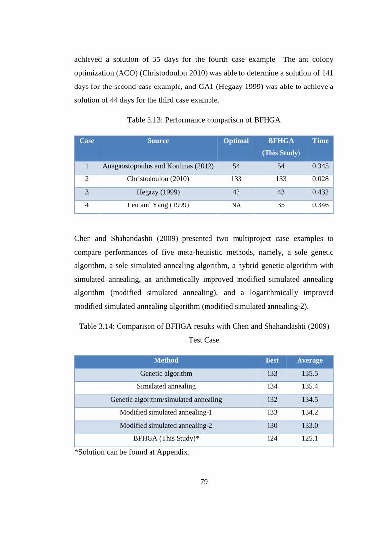
79
achieved a solution of 35 days for the fourth case example The ant colony
optimization (ACO) (Christodoulou 2010) was able to determine a solution of 141
days for the second case example, and GA1 (Hegazy 1999) was able to achieve a
solution of 44 days for the third case example.
Table 3.13: Performance comparison of BFHGA
Case Source Optimal BFHGA
(This Study)
Time
1 Anagnostopoulos and Koulinas (2012) 54 54 0.345
2 Christodoulou (2010) 133 133 0.028
3 Hegazy (1999) 43 43 0.432
4 Leu and Yang (1999) NA 35 0.346
Chen and Shahandashti (2009) presented two multiproject case examples to
compare performances of five meta-heuristic methods, namely, a sole genetic
algorithm, a sole simulated annealing algorithm, a hybrid genetic algorithm with
simulated annealing, an arithmetically improved modified simulated annealing
algorithm (modified simulated annealing), and a logarithmically improved
modified simulated annealing algorithm (modified simulated annealing-2).
Table 3.14: Comparison of BFHGA results with Chen and Shahandashti (2009)
Test Case
Method Best Average
Genetic algorithm 133 135.5
Simulated annealing 134 135.4
Genetic algorithm/simulated annealing 132 134.5
Modified simulated annealing-1 133 134.2
Modified simulated annealing-2 130 133.0
BFHGA (This Study)* 124 125.1
*Solution can be found at Appendix.
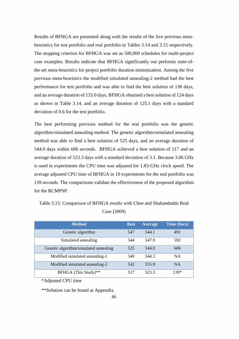
80
Results of BFHGA are presented along with the results of the five previous meta-
heuristics for test portfolio and real portfolio in Tables 3.14 and 3.15 respectively.
The stopping criterion for BFHGA was set as 500,000 schedules for multi-project
case examples. Results indicate that BFHGA significantly out performs state-of-
the-art meta-heuristics for project portfolio duration minimization. Among the five
previous meta-heuristics the modified simulated annealing-2 method had the best
performance for test portfolio and was able to find the best solution of 130 days,
and an average duration of 133.0 days. BFHGA obtained a best solution of 124 days
as shown in Table 3.14, and an average duration of 125.1 days with a standard
deviation of 0.6 for the test portfolio.
The best performing previous method for the real portfolio was the genetic
algorithm/simulated annealing method. The genetic algorithm/simulated annealing
method was able to find a best solution of 525 days, and an average duration of
544.0 days within 606 seconds. BFHGA achieved a best solution of 517 and an
average duration of 523.3 days with a standard deviation of 3.1. Because 3.06 GHz
is used in experiments the CPU time was adjusted for 1.83-GHz clock speed. The
average adjusted CPU time of BFHGA in 10 experiments for the real portfolio was
139 seconds. The comparisons validate the effectiveness of the proposed algorithm
for the RCMPSP.
Table 3.15: Comparison of BFHGA results with Chen and Shahandashti Real
Case (2009)
Method Best Average Time (Secs)
Genetic algorithm 547 544.1 491
Simulated annealing 544 547.9 592
Genetic algorithm/simulated annealing 525 544.0 606
Modified simulated annealing-1 540 544.3 NA
Modified simulated annealing-2 542 555.9 NA
BFHGA (This Study)** 517 523.3 139*
*Adjusted CPU time
**Solution can be found at Appendix.
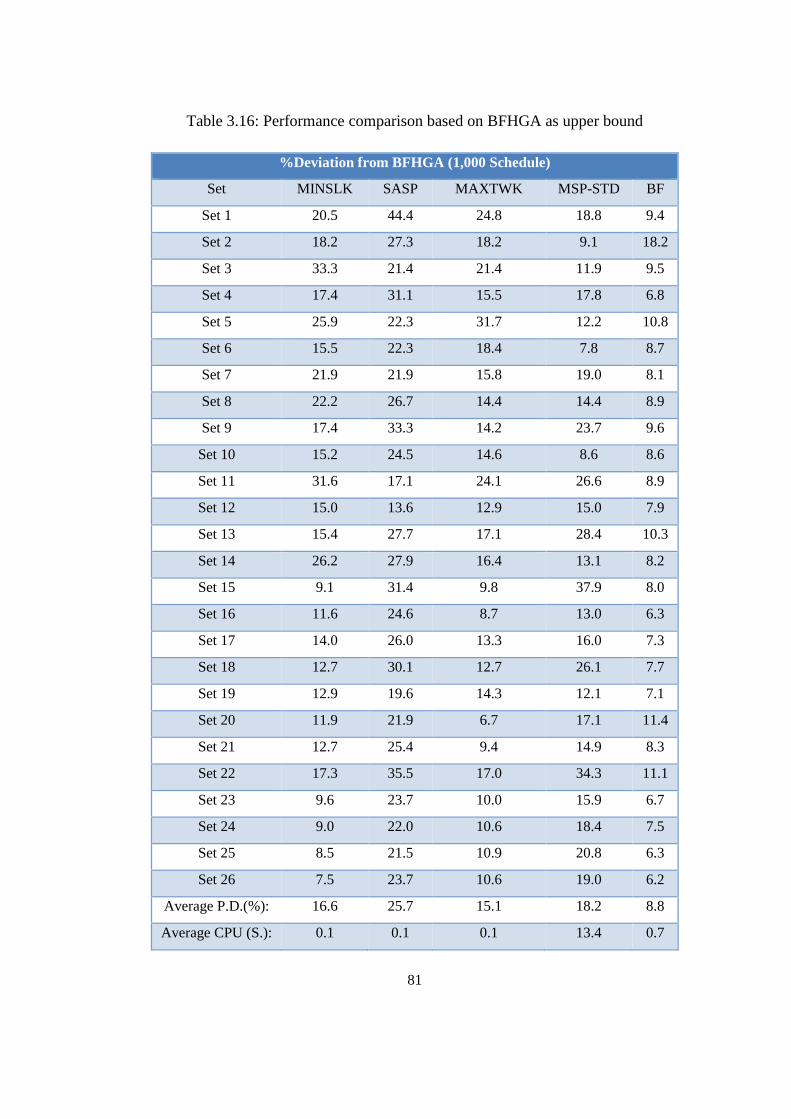
81
Table 3.16: Performance comparison based on BFHGA as upper bound
%Deviation from BFHGA (1,000 Schedule)
Set MINSLK SASP MAXTWK MSP-STD BF
Set 1 20.5 44.4 24.8 18.8 9.4
Set 2 18.2 27.3 18.2 9.1 18.2
Set 3 33.3 21.4 21.4 11.9 9.5
Set 4 17.4 31.1 15.5 17.8 6.8
Set 5 25.9 22.3 31.7 12.2 10.8
Set 6 15.5 22.3 18.4 7.8 8.7
Set 7 21.9 21.9 15.8 19.0 8.1
Set 8 22.2 26.7 14.4 14.4 8.9
Set 9 17.4 33.3 14.2 23.7 9.6
Set 10 15.2 24.5 14.6 8.6 8.6
Set 11 31.6 17.1 24.1 26.6 8.9
Set 12 15.0 13.6 12.9 15.0 7.9
Set 13 15.4 27.7 17.1 28.4 10.3
Set 14 26.2 27.9 16.4 13.1 8.2
Set 15 9.1 31.4 9.8 37.9 8.0
Set 16 11.6 24.6 8.7 13.0 6.3
Set 17 14.0 26.0 13.3 16.0 7.3
Set 18 12.7 30.1 12.7 26.1 7.7
Set 19 12.9 19.6 14.3 12.1 7.1
Set 20 11.9 21.9 6.7 17.1 11.4
Set 21 12.7 25.4 9.4 14.9 8.3
Set 22 17.3 35.5 17.0 34.3 11.1
Set 23 9.6 23.7 10.0 15.9 6.7
Set 24 9.0 22.0 10.6 18.4 7.5
Set 25 8.5 21.5 10.9 20.8 6.3
Set 26 7.5 23.7 10.6 19.0 6.2
Average P.D.(%): 16.6 25.7 15.1 18.2 8.8
Average CPU (S.): 0.1 0.1 0.1 13.4 0.7
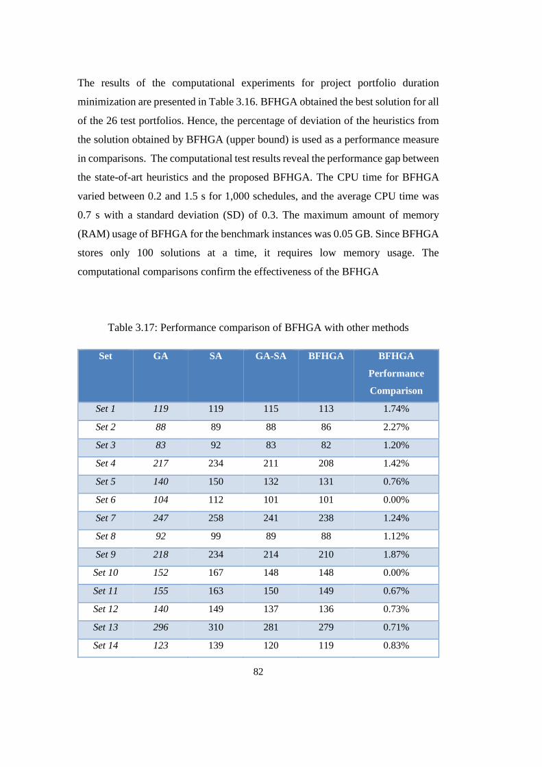
82
The results of the computational experiments for project portfolio duration
minimization are presented in Table 3.16. BFHGA obtained the best solution for all
of the 26 test portfolios. Hence, the percentage of deviation of the heuristics from
the solution obtained by BFHGA (upper bound) is used as a performance measure
in comparisons. The computational test results reveal the performance gap between
the state-of-art heuristics and the proposed BFHGA. The CPU time for BFHGA
varied between 0.2 and 1.5 s for 1,000 schedules, and the average CPU time was
0.7 s with a standard deviation (SD) of 0.3. The maximum amount of memory
(RAM) usage of BFHGA for the benchmark instances was 0.05 GB. Since BFHGA
stores only 100 solutions at a time, it requires low memory usage. The
computational comparisons confirm the effectiveness of the BFHGA
Table 3.17: Performance comparison of BFHGA with other methods
Set GA SA GA-SA BFHGA BFHGA
Performance
Comparison
Set 1 119 119 115 113 1.74%
Set 2 88 89 88 86 2.27%
Set 3 83 92 83 82 1.20%
Set 4 217 234 211 208 1.42%
Set 5 140 150 132 131 0.76%
Set 6 104 112 101 101 0.00%
Set 7 247 258 241 238 1.24%
Set 8 92 99 89 88 1.12%
Set 9 218 234 214 210 1.87%
Set 10 152 167 148 148 0.00%
Set 11 155 163 150 149 0.67%
Set 12 140 149 137 136 0.73%
Set 13 296 310 281 279 0.71%
Set 14 123 139 120 119 0.83%
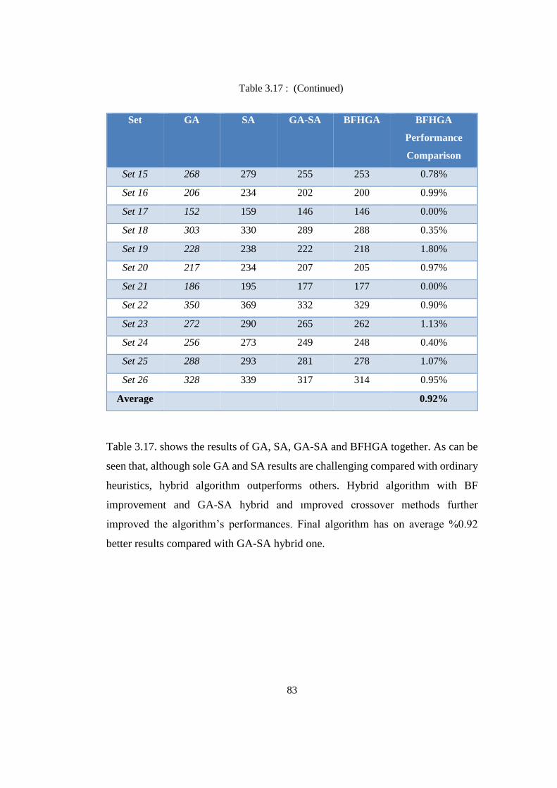
83
Set GA SA GA-SA BFHGA BFHGA
Performance
Comparison
Set 15 268 279 255 253 0.78%
Set 16 206 234 202 200 0.99%
Set 17 152 159 146 146 0.00%
Set 18 303 330 289 288 0.35%
Set 19 228 238 222 218 1.80%
Set 20 217 234 207 205 0.97%
Set 21 186 195 177 177 0.00%
Set 22 350 369 332 329 0.90%
Set 23 272 290 265 262 1.13%
Set 24 256 273 249 248 0.40%
Set 25 288 293 281 278 1.07%
Set 26 328 339 317 314 0.95%
Average 0.92%
Table 3.17. shows the results of GA, SA, GA-SA and BFHGA together. As can be
seen that, although sole GA and SA results are challenging compared with ordinary
heuristics, hybrid algorithm outperforms others. Hybrid algorithm with BF
improvement and GA-SA hybrid and ımproved crossover methods further
improved the algorithm’s performances. Final algorithm has on average %0.92
better results compared with GA-SA hybrid one.
Table 3.17 : (Continued)
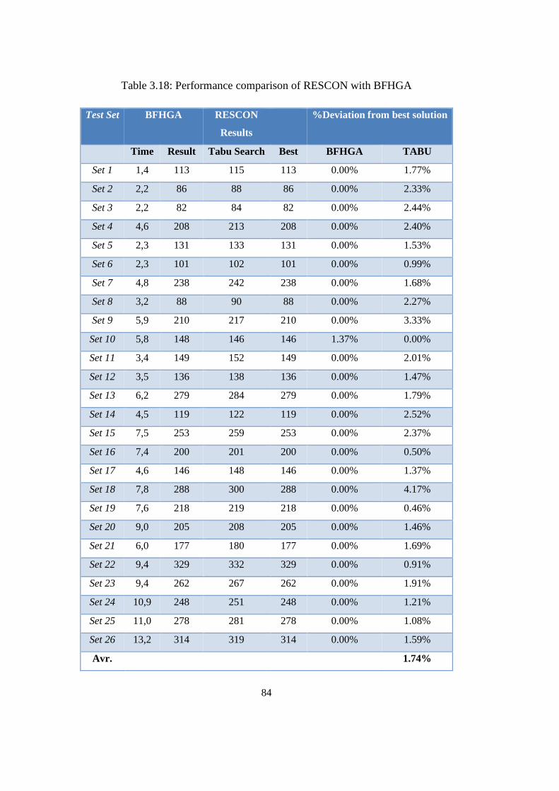
84
Table 3.18: Performance comparison of RESCON with BFHGA
Test Set BFHGA RESCON
Results
%Deviation from best solution
Time Result Tabu Search Best BFHGA TABU
Set 1 1,4 113 115 113 0.00% 1.77%
Set 2 2,2 86 88 86 0.00% 2.33%
Set 3 2,2 82 84 82 0.00% 2.44%
Set 4 4,6 208 213 208 0.00% 2.40%
Set 5 2,3 131 133 131 0.00% 1.53%
Set 6 2,3 101 102 101 0.00% 0.99%
Set 7 4,8 238 242 238 0.00% 1.68%
Set 8 3,2 88 90 88 0.00% 2.27%
Set 9 5,9 210 217 210 0.00% 3.33%
Set 10 5,8 148 146 146 1.37% 0.00%
Set 11 3,4 149 152 149 0.00% 2.01%
Set 12 3,5 136 138 136 0.00% 1.47%
Set 13 6,2 279 284 279 0.00% 1.79%
Set 14 4,5 119 122 119 0.00% 2.52%
Set 15 7,5 253 259 253 0.00% 2.37%
Set 16 7,4 200 201 200 0.00% 0.50%
Set 17 4,6 146 148 146 0.00% 1.37%
Set 18 7,8 288 300 288 0.00% 4.17%
Set 19 7,6 218 219 218 0.00% 0.46%
Set 20 9,0 205 208 205 0.00% 1.46%
Set 21 6,0 177 180 177 0.00% 1.69%
Set 22 9,4 329 332 329 0.00% 0.91%
Set 23 9,4 262 267 262 0.00% 1.91%
Set 24 10,9 248 251 248 0.00% 1.21%
Set 25 11,0 278 281 278 0.00% 1.08%
Set 26 13,2 314 319 314 0.00% 1.59%
Avr. 1.74%
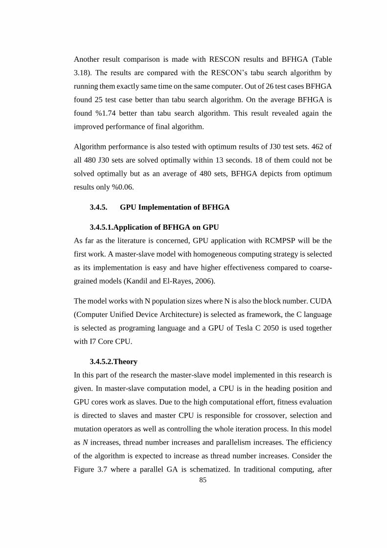
85
Another result comparison is made with RESCON results and BFHGA (Table
3.18). The results are compared with the RESCON’s tabu search algorithm by
running them exactly same time on the same computer. Out of 26 test cases BFHGA
found 25 test case better than tabu search algorithm. On the average BFHGA is
found %1.74 better than tabu search algorithm. This result revealed again the
improved performance of final algorithm.
Algorithm performance is also tested with optimum results of J30 test sets. 462 of
all 480 J30 sets are solved optimally within 13 seconds. 18 of them could not be
solved optimally but as an average of 480 sets, BFHGA depicts from optimum
results only %0.06.
3.4.5. GPU Implementation of BFHGA
3.4.5.1.Application of BFHGA on GPU
As far as the literature is concerned, GPU application with RCMPSP will be the
first work. A master-slave model with homogeneous computing strategy is selected
as its implementation is easy and have higher effectiveness compared to coarse-
grained models (Kandil and El-Rayes, 2006).
The model works with N population sizes where N is also the block number. CUDA
(Computer Unified Device Architecture) is selected as framework, the C language
is selected as programing language and a GPU of Tesla C 2050 is used together
with I7 Core CPU.
3.4.5.2.Theory
In this part of the research the master-slave model implemented in this research is
given. In master-slave computation model, a CPU is in the heading position and
GPU cores work as slaves. Due to the high computational effort, fitness evaluation
is directed to slaves and master CPU is responsible for crossover, selection and
mutation operators as well as controlling the whole iteration process. In this model
as N increases, thread number increases and parallelism increases. The efficiency
of the algorithm is expected to increase as thread number increases. Consider the
Figure 3.7 where a parallel GA is schematized. In traditional computing, after
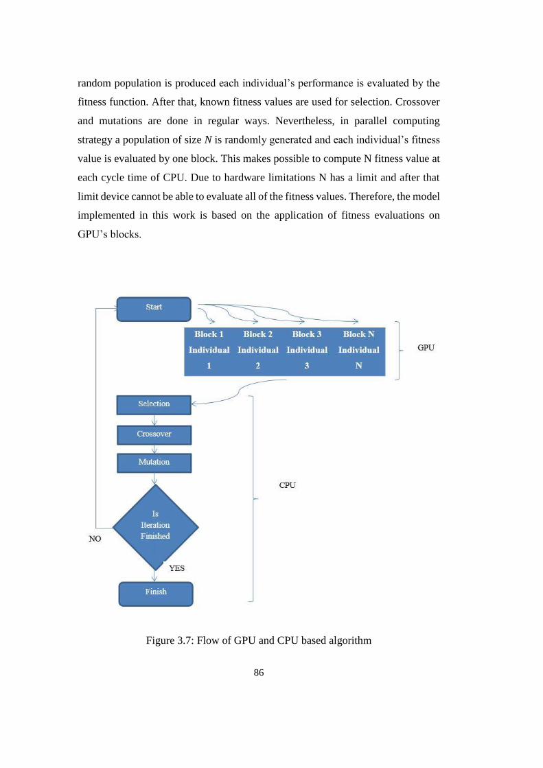
86
random population is produced each individual’s performance is evaluated by the
fitness function. After that, known fitness values are used for selection. Crossover
and mutations are done in regular ways. Nevertheless, in parallel computing
strategy a population of size N is randomly generated and each individual’s fitness
value is evaluated by one block. This makes possible to compute N fitness value at
each cycle time of CPU. Due to hardware limitations N has a limit and after that
limit device cannot be able to evaluate all of the fitness values. Therefore, the model
implemented in this work is based on the application of fitness evaluations on
GPU’s blocks.
Figure 3.7: Flow of GPU and CPU based algorithm
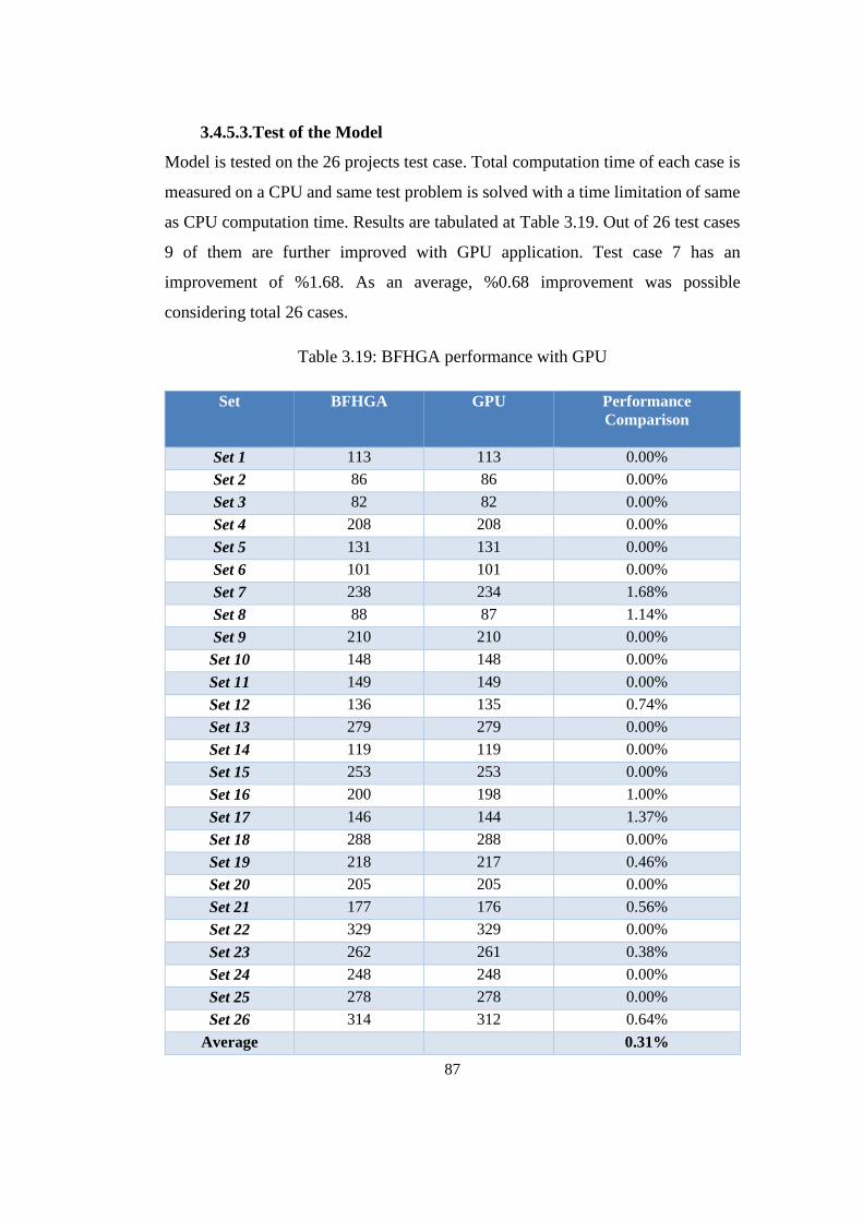
87
3.4.5.3.Test of the Model
Model is tested on the 26 projects test case. Total computation time of each case is
measured on a CPU and same test problem is solved with a time limitation of same
as CPU computation time. Results are tabulated at Table 3.19. Out of 26 test cases
9 of them are further improved with GPU application. Test case 7 has an
improvement of %1.68. As an average, %0.68 improvement was possible
considering total 26 cases.
Table 3.19: BFHGA performance with GPU
Set BFHGA GPU Performance
Comparison
Set 1 113 113 0.00%
Set 2 86 86 0.00%
Set 3 82 82 0.00%
Set 4 208 208 0.00%
Set 5 131 131 0.00%
Set 6 101 101 0.00%
Set 7 238 234 1.68%
Set 8 88 87 1.14%
Set 9 210 210 0.00%
Set 10 148 148 0.00%
Set 11 149 149 0.00%
Set 12 136 135 0.74%
Set 13 279 279 0.00%
Set 14 119 119 0.00%
Set 15 253 253 0.00%
Set 16 200 198 1.00%
Set 17 146 144 1.37%
Set 18 288 288 0.00%
Set 19 218 217 0.46%
Set 20 205 205 0.00%
Set 21 177 176 0.56%
Set 22 329 329 0.00%
Set 23 262 261 0.38%
Set 24 248 248 0.00%
Set 25 278 278 0.00%
Set 26 314 312 0.64%
Average 0.31%
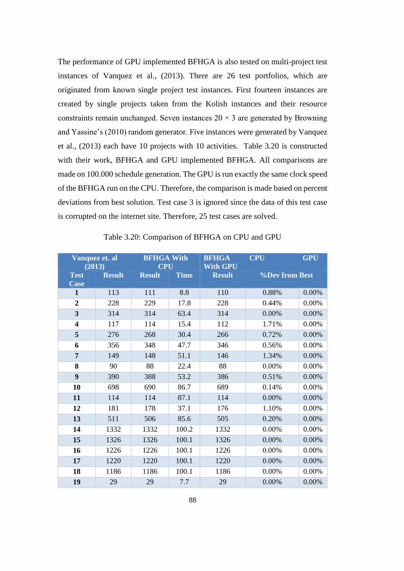
88
The performance of GPU implemented BFHGA is also tested on multi-project test
instances of Vanquez et al., (2013). There are 26 test portfolios, which are
originated from known single project test instances. First fourteen instances are
created by single projects taken from the Kolish instances and their resource
constraints remain unchanged. Seven instances 20 × 3 are generated by Browning
and Yassine’s (2010) random generator. Five instances were generated by Vanquez
et al., (2013) each have 10 projects with 10 activities. Table 3.20 is constructed
with their work, BFHGA and GPU implemented BFHGA. All comparisons are
made on 100.000 schedule generation. The GPU is run exactly the same clock speed
of the BFHGA run on the CPU. Therefore, the comparison is made based on percent
deviations from best solution. Test case 3 is ignored since the data of this test case
is corrupted on the internet site. Therefore, 25 test cases are solved.
Table 3.20: Comparison of BFHGA on CPU and GPU
Vanquez et. al
(2013)
BFHGA With
CPU
BFHGA
With GPU
CPU GPU
Test
Case
Result Result Time Result %Dev from Best
1 113 111 8.8 110 0.88% 0.00%
2 228 229 17.8 228 0.44% 0.00%
3 314 314 63.4 314 0.00% 0.00%
4 117 114 15.4 112 1.71% 0.00%
5 276 268 30.4 266 0.72% 0.00%
6 356 348 47.7 346 0.56% 0.00%
7 149 148 51.1 146 1.34% 0.00%
8 90 88 22.4 88 0.00% 0.00%
9 390 388 53.2 386 0.51% 0.00%
10 698 690 86.7 689 0.14% 0.00%
11 114 114 87.1 114 0.00% 0.00%
12 181 178 37.1 176 1.10% 0.00%
13 511 506 85.6 505 0.20% 0.00%
14 1332 1332 100.2 1332 0.00% 0.00%
15 1326 1326 100.1 1326 0.00% 0.00%
16 1226 1226 100.1 1226 0.00% 0.00%
17 1220 1220 100.1 1220 0.00% 0.00%
18 1186 1186 100.1 1186 0.00% 0.00%
19 29 29 7.7 29 0.00% 0.00%
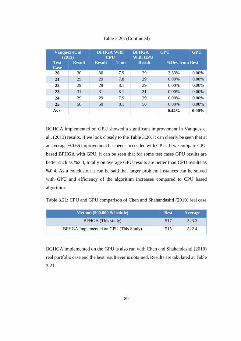
89
Vanquez et. al
(2013)
BFHGA With
CPU
BFHGA
With GPU
CPU GPU
Test
Case
Result Result Time Result %Dev from Best
20 30 30 7.9 29 3.33% 0.00%
21 29 29 7.8 29 0.00% 0.00%
22 29 29 8.1 29 0.00% 0.00%
23 31 31 8.1 31 0.00% 0.00%
24 29 29 7.9 29 0.00% 0.00%
25 50 50 8.1 50 0.00% 0.00%
Avr. 0.44% 0.00%
BGHGA implemented on GPU showed a significant improvement in Vanquez et
al., (2013) results. If we look closely to the Table 3.20. It can clearly be seen that at
an average %0.65 improvement has been succeeded with CPU. If we compare CPU
based BFHGA with GPU, it can be seen that for some test cases GPU results are
better such as %3.3, totally on average GPU results are better than CPU results as
%0.4. As a conclusion it can be said that larger problem instances can be solved
with GPU and efficiency of the algorithm increases compared to CPU based
algorithm.
Table 3.21: CPU and GPU comparison of Chen and Shahandashti (2010) real case
Method (500.000 Schedule) Best Average
BFHGA (This study) 517 523.3
BFHGA Implemented on GPU (This Study) 515 522.4
BGHGA implemented on the GPU is also run with Chen and Shahandashti (2010)
real portfolio case and the best result ever is obtained. Results are tabulated at Table
3.21.
Table 3.20: (Continued)
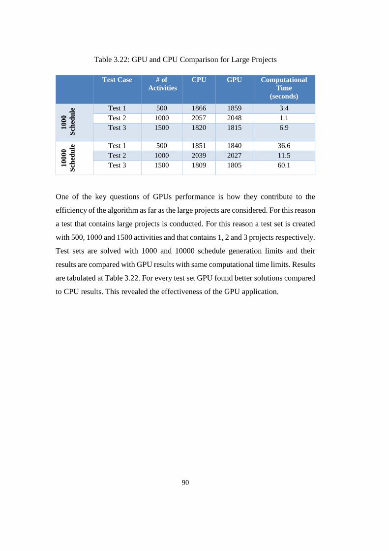
90
Table 3.22: GPU and CPU Comparison for Large Projects
Test Case # of
Activities
CPU GPU Computational
Time
(seconds)
10
00
Sch
edu
le Test 1 500 1866 1859 3.4
Test 2 1000 2057 2048 1.1
Test 3 1500 1820 1815 6.9
10
00
0
Sch
edu
le
Test 1 500 1851 1840 36.6
Test 2 1000 2039 2027 11.5
Test 3 1500 1809 1805 60.1
One of the key questions of GPUs performance is how they contribute to the
efficiency of the algorithm as far as the large projects are considered. For this reason
a test that contains large projects is conducted. For this reason a test set is created
with 500, 1000 and 1500 activities and that contains 1, 2 and 3 projects respectively.
Test sets are solved with 1000 and 10000 schedule generation limits and their
results are compared with GPU results with same computational time limits. Results
are tabulated at Table 3.22. For every test set GPU found better solutions compared
to CPU results. This revealed the effectiveness of the GPU application.
91
CHAPTER 4
4. ANALYSIS OF ALGORITHM PARAMETERS
Meta-heuristics’ power comes from the iteration process and the capability to
search the domain effectively. Although stochastic nature of the meta-heuristics
gives an extra power to explore the domain extensively, validity of the algorithm is
also important. In order to analyze the behavior of the algorithm with various
parameters, it is important to analyze their effects. Analyzing the effects of
parameters and design them in order to optimize meta-heuristics’ parameters is not
only an ad hoc process but also requires some statistics. Some conventions are used
extensively such as high population size and low mutation rate etc. Thus, there is
not an exact solution to optimize the parameters and fine tune them.
In this chapter it is intended to make an experiment design in order to obtain as
much information as possible on the parameters and its effects on algorithm
performance. Since boundary of the parameters can be set as minimum and
maximum, two level factorial design procedures is selected. Main advantage of
factorial design is the ability to understand parameter effects solely and
simultaneously with the minimum and maximum parameter settings.
4.1.Two Level Factorial Design
4.1.1. Theory:
Aim of a factorial design is to measure systematically the output and to test the
validity of the experiment. Parameters are changed in a systematical way and the
response of the algorithm is measured. The lower level of an input parameter is
usually indicated with a `-' sign; the higher level with a `+' sign.
Basic case of a factorial design is to measure the effect of one variable. If one
variable and its effect is considered the model becomes a linear model as follows;
Assuming the output of a model with Y and parameter with X;
92
𝑌 = 𝛽0 + 𝛽1𝑋 (4.1)
Effect of a parameter is defined as the difference in the average response between
the high and low levels of a factor.
The main effect of X is modelled in this way;
𝐸 (𝑋) = 𝑌𝑋+ − 𝑌𝑋− (4.2)
Variance of N observations can be modelled such as;
𝑉𝑎𝑟 (𝑋) =4
𝑁𝜎2 (4.3)
As more parameters are considered the model becomes more complex. If more than
one parameter is considered both the effects of each variable and their interactions
should be taken into account and experiment number increases exponentially such
that if there is 2 level and k dependent variable there should be 2k number of
experiments in order to make a factorial design.
2k factorial design is used extensively in the early stages of an experiment where
the effects of dependent variables are investigated. Since two level of factor is
considered, response is assumed to be linear over the range (Montgomery D.C.,
p.233, 2012).
For two level and two variables, interaction is defined as one-half of the difference
between the effect of parameter X1 at the high level of X2 and the effect of X1 at the
low level of X2.
The effect of two dependent variables is modelled in this way;
𝐸(𝑋1, 𝑋2) = 1
2[(𝑌𝑥1+
− 𝑌𝑥1−)
𝑋2+
− (𝑌𝑥1+− 𝑌𝑥1−
)𝑋2−
] (4.4)
where inside double brackets is called contrast of treatment (Montgomery D.C.,
p.244, 2012).
93
If we consider more than two variables, it is necessary to use design matrix which
makes easier to measure the variable effects. To measure the effect of any factor,
matrix can be used according to signs designated at the each cell M[i] [j] .
For example:
Effect of variable A and AB is calculated easily considering design matrix such as:
𝐴 =1
8[𝑎 − 𝑇 − 𝑏 + 𝑎𝑏 − 𝑐 + 𝑎𝑐 − 𝑏𝑐 + 𝑎𝑏𝑐 − 𝑑 + 𝑎𝑑 − 𝑏𝑑 + 𝑎𝑏𝑑 − 𝑐𝑑 + 𝑎𝑐𝑑
− 𝑏𝑐𝑑 + 𝑎𝑏𝑐𝑑]
𝐴𝐵 =1
8[𝑇 − 𝑎 − 𝑏 + 𝑎𝑏 + 𝑐 − 𝑎𝑐 − 𝑏𝑐 + 𝑎𝑏𝑐 + 𝑑 − 𝑎𝑑 − 𝑏𝑑 + 𝑎𝑏𝑑 + 𝑐𝑑
− 𝑎𝑐𝑑 − 𝑏𝑐𝑑 + 𝑎𝑏𝑐𝑑]
Sum of square of any factor is calculated as:
𝑆𝑆𝑖𝑗 =1
2𝑘 (𝐶𝑜𝑛𝑡𝑟𝑎𝑠𝑡𝑖𝑗)2 (4.5)
Mean square error is calculated as:
𝑀𝑆𝐸𝑖𝑗 =𝑆𝑆𝑖𝑗
𝐷𝑜𝑓𝑖𝑗 (4.6)
Finally F value is calculated as:
𝐹 =𝑀𝑆𝐸𝑖𝑗
𝑀𝑆𝐸𝑒𝑟𝑟𝑜𝑟 (4.7)
A half normal graph is obtained using the experiment results. Cumulative
distribution of observed effects can be used for interpretation of each variable. If a
half normal plot paper is used only probability for each test and their effects are
drawn. Otherwise if plot paper is not available effects are converted to z values.
Main factors can easily be determined since they exist as outliers. All effects lie
along trend line are negligible whereas outliers have significant effects.
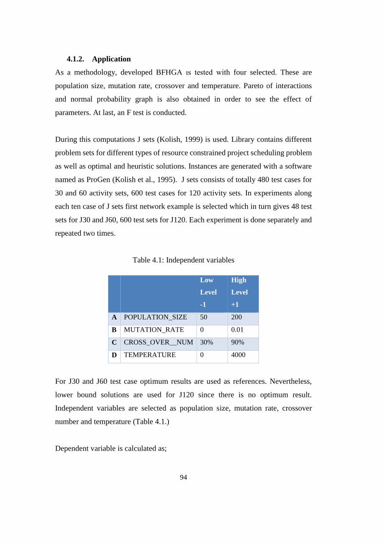
94
4.1.2. Application
As a methodology, developed BFHGA ıs tested with four selected. These are
population size, mutation rate, crossover and temperature. Pareto of interactions
and normal probability graph is also obtained in order to see the effect of
parameters. At last, an F test is conducted.
During this computations J sets (Kolish, 1999) is used. Library contains different
problem sets for different types of resource constrained project scheduling problem
as well as optimal and heuristic solutions. Instances are generated with a software
named as ProGen (Kolish et al., 1995). J sets consists of totally 480 test cases for
30 and 60 activity sets, 600 test cases for 120 activity sets. In experiments along
each ten case of J sets first network example is selected which in turn gives 48 test
sets for J30 and J60, 600 test sets for J120. Each experiment is done separately and
repeated two times.
Table 4.1: Independent variables
Low
Level
-1
High
Level
+1
A POPULATION_SIZE 50 200
B MUTATION_RATE 0 0.01
C CROSS_OVER__NUM 30% 90%
D TEMPERATURE 0 4000
For J30 and J60 test case optimum results are used as references. Nevertheless,
lower bound solutions are used for J120 since there is no optimum result.
Independent variables are selected as population size, mutation rate, crossover
number and temperature (Table 4.1.)
Dependent variable is calculated as;
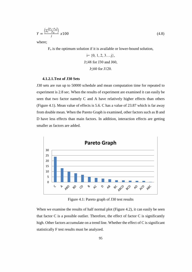
95
𝑌 =(∑
[𝐹𝑖−𝐹𝑜]
𝐹𝑜
𝑗𝑖 )
𝑗 𝑥100 (4.8)
where;
Fo is the optimum solution if it is available or lower-bound solution,
i= {0, 1, 2, 3….j},
J≤48 for J30 and J60,
J≤60 for J120.
4.1.2.1.Test of J30 Sets
J30 sets are run up to 50000 schedule and mean computation time for repeated to
experiment is 2.8 sec. When the results of experiment are examined it can easily be
seen that two factor namely C and A have relatively higher effects than others
(Figure 4.1). Mean value of effects is 5.6. C has a value of 23.87 which is far away
from double mean. When the Pareto Graph is examined, other factors such as B and
D have less effects than main factors. In addition, interaction effects are getting
smaller as factors are added.
Figure 4.1: Pareto graph of J30 test results
When we examine the results of half normal plot (Figure 4.2), it can easily be seen
that factor C is a possible outlier. Therefore, the effect of factor C is significantly
high. Other factors accumulate on a trend line. Whether the effect of C is significant
statistically F test results must be analyzed.
0
5
10
15
20
25
30
Pareto Graph
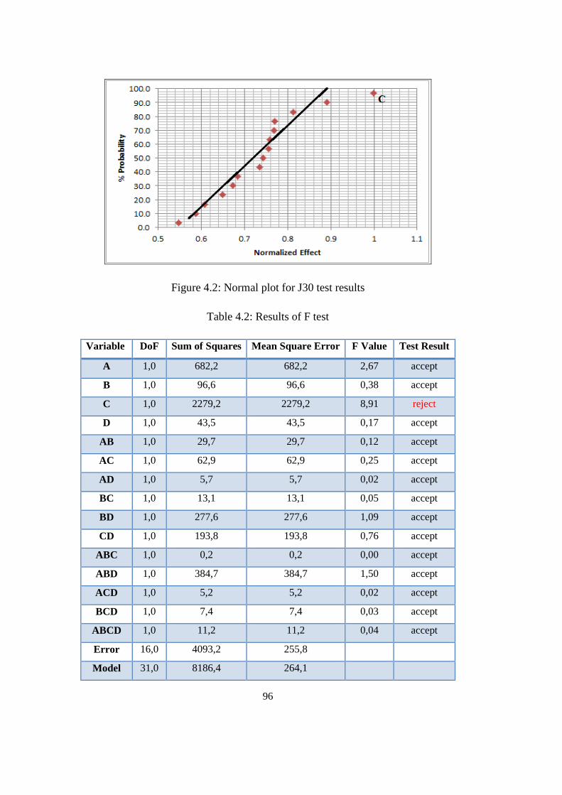
96
Figure 4.2: Normal plot for J30 test results
Table 4.2: Results of F test
Variable DoF Sum of Squares Mean Square Error F Value Test Result
A 1,0 682,2 682,2 2,67 accept
B 1,0 96,6 96,6 0,38 accept
C 1,0 2279,2 2279,2 8,91 reject
D 1,0 43,5 43,5 0,17 accept
AB 1,0 29,7 29,7 0,12 accept
AC 1,0 62,9 62,9 0,25 accept
AD 1,0 5,7 5,7 0,02 accept
BC 1,0 13,1 13,1 0,05 accept
BD 1,0 277,6 277,6 1,09 accept
CD 1,0 193,8 193,8 0,76 accept
ABC 1,0 0,2 0,2 0,00 accept
ABD 1,0 384,7 384,7 1,50 accept
ACD 1,0 5,2 5,2 0,02 accept
BCD 1,0 7,4 7,4 0,03 accept
ABCD 1,0 11,2 11,2 0,04 accept
Error 16,0 4093,2 255,8
Model 31,0 8186,4 264,1
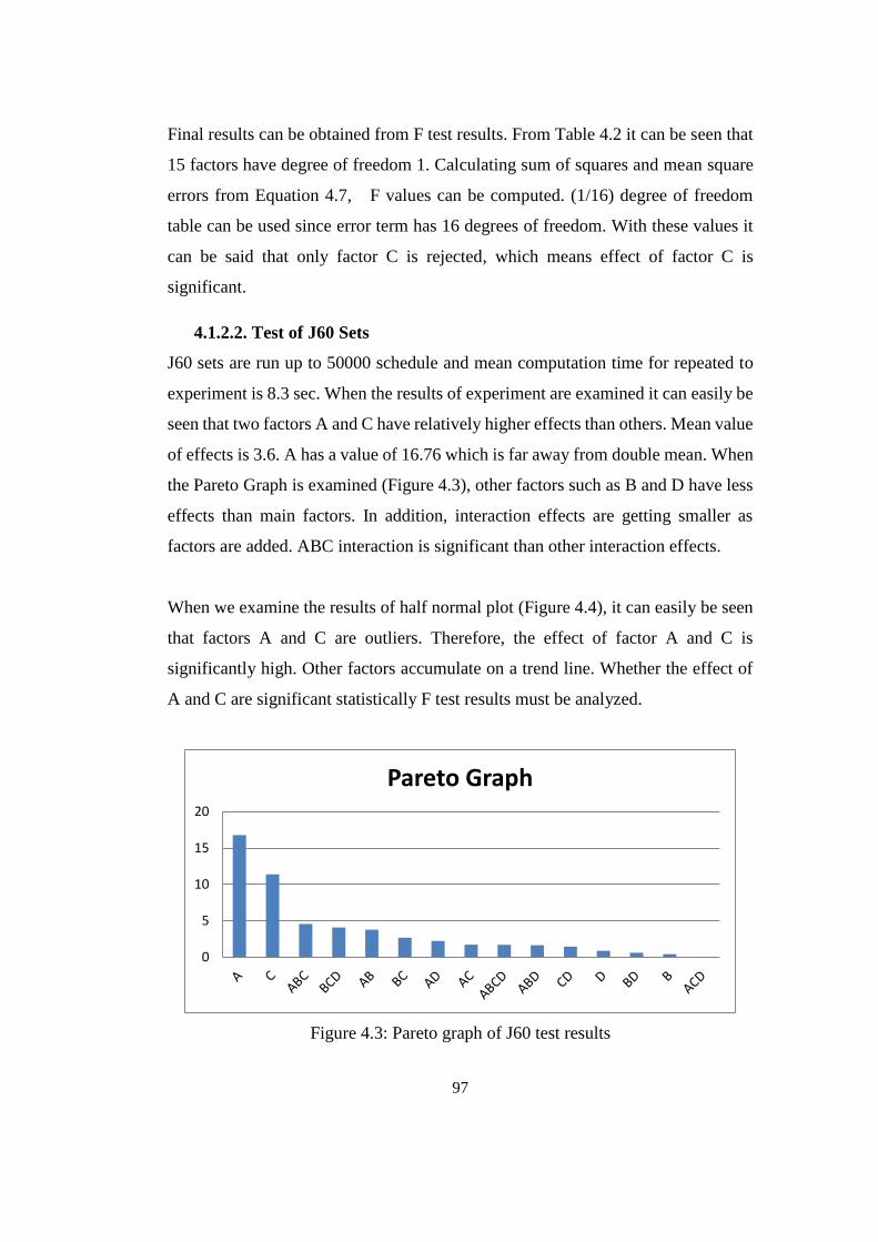
97
Final results can be obtained from F test results. From Table 4.2 it can be seen that
15 factors have degree of freedom 1. Calculating sum of squares and mean square
errors from Equation 4.7, F values can be computed. (1/16) degree of freedom
table can be used since error term has 16 degrees of freedom. With these values it
can be said that only factor C is rejected, which means effect of factor C is
significant.
4.1.2.2. Test of J60 Sets
J60 sets are run up to 50000 schedule and mean computation time for repeated to
experiment is 8.3 sec. When the results of experiment are examined it can easily be
seen that two factors A and C have relatively higher effects than others. Mean value
of effects is 3.6. A has a value of 16.76 which is far away from double mean. When
the Pareto Graph is examined (Figure 4.3), other factors such as B and D have less
effects than main factors. In addition, interaction effects are getting smaller as
factors are added. ABC interaction is significant than other interaction effects.
When we examine the results of half normal plot (Figure 4.4), it can easily be seen
that factors A and C are outliers. Therefore, the effect of factor A and C is
significantly high. Other factors accumulate on a trend line. Whether the effect of
A and C are significant statistically F test results must be analyzed.
Figure 4.3: Pareto graph of J60 test results
0
5
10
15
20
Pareto Graph
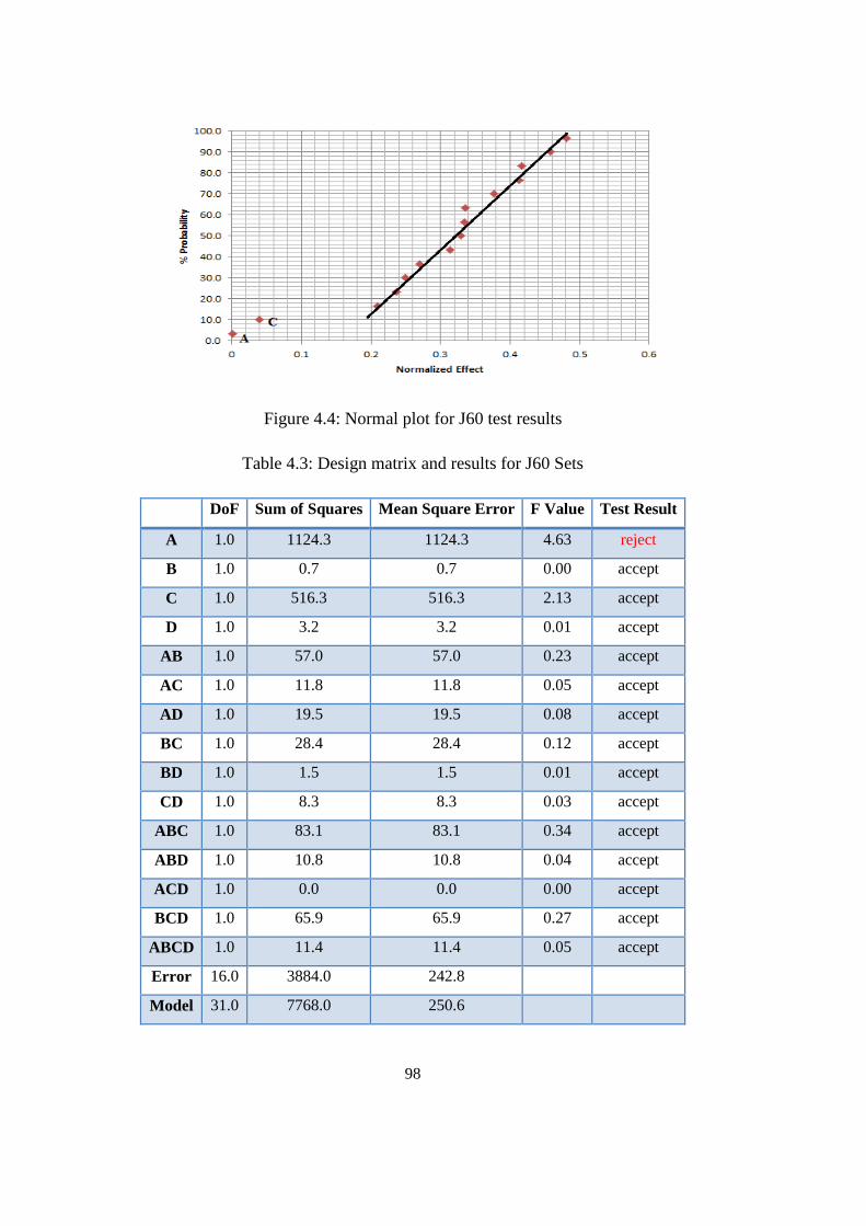
98
Figure 4.4: Normal plot for J60 test results
Table 4.3: Design matrix and results for J60 Sets
DoF Sum of Squares Mean Square Error F Value Test Result
A 1.0 1124.3 1124.3 4.63 reject
B 1.0 0.7 0.7 0.00 accept
C 1.0 516.3 516.3 2.13 accept
D 1.0 3.2 3.2 0.01 accept
AB 1.0 57.0 57.0 0.23 accept
AC 1.0 11.8 11.8 0.05 accept
AD 1.0 19.5 19.5 0.08 accept
BC 1.0 28.4 28.4 0.12 accept
BD 1.0 1.5 1.5 0.01 accept
CD 1.0 8.3 8.3 0.03 accept
ABC 1.0 83.1 83.1 0.34 accept
ABD 1.0 10.8 10.8 0.04 accept
ACD 1.0 0.0 0.0 0.00 accept
BCD 1.0 65.9 65.9 0.27 accept
ABCD 1.0 11.4 11.4 0.05 accept
Error 16.0 3884.0 242.8
Model 31.0 7768.0 250.6
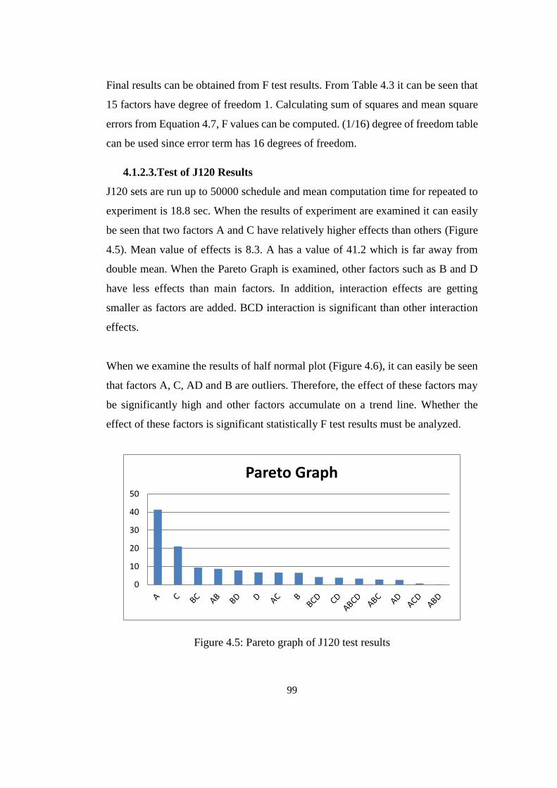
99
Final results can be obtained from F test results. From Table 4.3 it can be seen that
15 factors have degree of freedom 1. Calculating sum of squares and mean square
errors from Equation 4.7, F values can be computed. (1/16) degree of freedom table
can be used since error term has 16 degrees of freedom.
4.1.2.3.Test of J120 Results
J120 sets are run up to 50000 schedule and mean computation time for repeated to
experiment is 18.8 sec. When the results of experiment are examined it can easily
be seen that two factors A and C have relatively higher effects than others (Figure
4.5). Mean value of effects is 8.3. A has a value of 41.2 which is far away from
double mean. When the Pareto Graph is examined, other factors such as B and D
have less effects than main factors. In addition, interaction effects are getting
smaller as factors are added. BCD interaction is significant than other interaction
effects.
When we examine the results of half normal plot (Figure 4.6), it can easily be seen
that factors A, C, AD and B are outliers. Therefore, the effect of these factors may
be significantly high and other factors accumulate on a trend line. Whether the
effect of these factors is significant statistically F test results must be analyzed.
Figure 4.5: Pareto graph of J120 test results
0
10
20
30
40
50
Pareto Graph
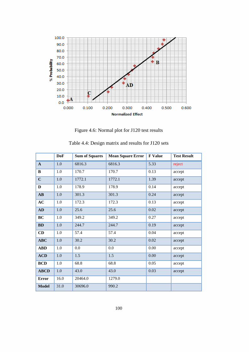
100
Figure 4.6: Normal plot for J120 test results
Table 4.4: Design matrix and results for J120 sets
DoF Sum of Squares Mean Square Error F Value Test Result
A 1.0 6816.3 6816.3 5.33 reject
B 1.0 170.7 170.7 0.13 accept
C 1.0 1772.1 1772.1 1.39 accept
D 1.0 178.9 178.9 0.14 accept
AB 1.0 301.3 301.3 0.24 accept
AC 1.0 172.3 172.3 0.13 accept
AD 1.0 25.6 25.6 0.02 accept
BC 1.0 349.2 349.2 0.27 accept
BD 1.0 244.7 244.7 0.19 accept
CD 1.0 57.4 57.4 0.04 accept
ABC 1.0 30.2 30.2 0.02 accept
ABD 1.0 0.0 0.0 0.00 accept
ACD 1.0 1.5 1.5 0.00 accept
BCD 1.0 68.8 68.8 0.05 accept
ABCD 1.0 43.0 43.0 0.03 accept
Error 16.0 20464.0 1279.0
Model 31.0 30696.0 990.2
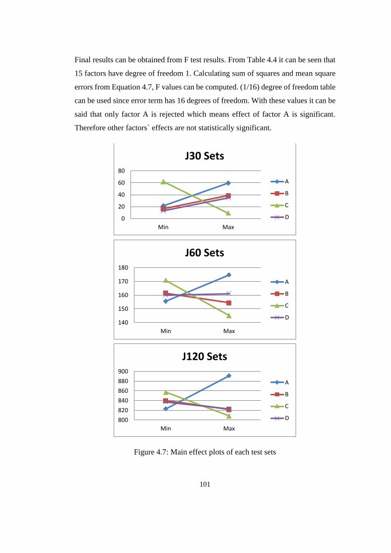
101
Final results can be obtained from F test results. From Table 4.4 it can be seen that
15 factors have degree of freedom 1. Calculating sum of squares and mean square
errors from Equation 4.7, F values can be computed. (1/16) degree of freedom table
can be used since error term has 16 degrees of freedom. With these values it can be
said that only factor A is rejected which means effect of factor A is significant.
Therefore other factors` effects are not statistically significant.
Figure 4.7: Main effect plots of each test sets
0
20
40
60
80
Min Max
J30 Sets
A
B
C
D
140
150
160
170
180
Min Max
J60 Sets
A
B
C
D
800
820
840
860
880
900
Min Max
J120 Sets
A
B
C
D

102
4.1.1. Interpretation from Main Effect Plots
A rough estimation of effects can also be seen from main effect plots. Main effect
of a factor is calculated when it is minimum while the others are maximum and
maximum while others are minimum. When the Figure 4.7 is considered effect of
A and C are looks similar. Increasing A and C would increase the effects
significantly. Whereas factors B and D behave different for each test case. For test
case J30, if B increases result would be incresing on the other hand for test case
J60 and J120 result would be decreasing with incresing value of B. As for factor
D, if it increases for J30 tests effects would be increasing, for J60 tests effects would
not change significantly and for J120 sets effects would be decreasing. It can be
concluded that for every test sets different parameter combinations should be used
in order to gain maximum benefit from the algorithm. It is also worth saying that
high population size, low mutation number, low crossover ratio would contribute
higher effects. Temperature parameter is not that significant but, rather it has fine
tuning capability.
103
CHAPTER 5
5. CONCLUSION
5.1. Summary and Discussion of Results
Effective resource management is vital in project management since idle resources
or excess resources increase the cost of the projects. Due to the challenging market
conditions and competition between companies, resource management process
becomes more important since cost overruns would result profit loss of the
company. This situation is well known in the construction sector but, practically
used techniques such as CPM does not cover resource management related issues.
Moreover, practically used software packages are neither capable of dealing with
multiple projects and its resources, nor have sufficient performances.
Resource allocation process which is extensively worked in operations research and
project management literature gives some directions to the practitioners through
heuristic methods, available software packages and developed algorithms.
However, majority of the existing research has focused on single projects. The
performances of these methods and software packages can be argued. Fast and
robust algorithms should be developed and this gap gives opportunities to the
researchers. Therefore, in this research it is aimed to obtain optimum or near
optimum solutions to the RCMPSP via meta-heuristics. For this purpose, a new
meta-heuristic algorithm was developed and its performance is tested with known
test instances. Developed algorithm is based on GA, SA and backward forward
heuristics through with improvements on mutations, crossover and selection
methods. Moreover, in order to increase the effectiveness of the algorithm parallel
computing strategy is applied to the algorithm and it is used with a GPU. The results
revealed the effectiveness of the algorithm.
Research has four main phases. In the first phase, a linear-integer model is
developed and it is tested with the previous test results. Also, it is shown that for
networks larger than 60 activities, linear-integer models are not capable of solving
the problem. It has been shown that software packages used extensively in the
104
practice have very low resource management capabilities. The second phase is the
algorithm development processes. It includes GA, SA, hybridization process and
new novel contributions to the algorithm. In order to clarify the development
process each part of the algorithm is summarized in corresponding sections. Third
phase is the performance measurement of the algorithms. Heuristics and known test
results are used for comparison purposes. Last phase is the parallel computing
application of final algorithm.
As a summary, the developed mathematical model is tested with optimum results
or upper bound solutions available in the literature. Standard Kolish (Kolisch and
Sprecher, 1997) test instance are used. Total time is limited to 300 seconds for J30
sets and 1000 seconds for j60 sets. J30 sets are completely solved with this model
and %94.5 of the results are optimum. %73 of J60 sets are solved optimally within
time and mean CPU time for Intel Core I5 computer is 14.3 and 19.9 seconds for
J30 and J60 sets respectively. J120 test sets cannot be solved within reasonable time
limits. Those sets cannot be solved optimally compared with upper bound solutions
and on the average, our model results depict from optimum and upper-bounds only
%2. 68. Most important conclusion of the model is the limitation of the
mathematical models for larger sets which is compatible with literature findings.
In order to test algorithms’ performances a heuristic solver was developed. In this
solver Minimum Slack (MinSlack), Shortest Activity from Shortest Project (SASP)
and Maximum Total Work Content (MaxTWK) heuristics are used. Also BF
heuristic is applied for each problem and results are compared within heuristics and
with meta-heuristics in further sections. BF heuristics outperformed other
heuristics.
A sole GA is developed with random key based chromosome representation. This
representation has been seldom used in the literature. Nevertheless, it has various
opportunities such as the fast crossover capability and compatibility with coding
techniques. It has been shown that even a sole GA is better %3.6 from best
heuristics with an average value of %7.04. In some test cases this value increases
up to %15.38. Developed GA is tested with MS Project’s heuristics. Test results
105
showed that in some test cases sole GA is better %26.37 with an average of %16.76.
Therefore, sole GA outperformed the known software packages’ heuristics.
A sole SA with the idea of worse solutions can also be accepted to some extend is
applied. The probability of accepting worse solutions is high at the beginning and
it is decreased according to a linear cooling schema. Results are compared with GA
results. It has been revealed that GA solutions performed better in all cases. GA on
the average performed %5.6 better. Since GA explores a large space compared to
SA, the results verified the effectiveness of GA.
A sole SA has a low search efficiency as it maintains only one solution at each
iteration. GA on the other hand, can contain knowledge of previous good solutions
and have high search capacity. An intelligent hybrid algorithm which has better
sides of each algorithm would perform better results. Therefore, a GA and SA
hybrid algorithm is developed and tested with sole GA and sole SA results. Results
revealed that the hybrid algorithm performance is better than sole algorithms and it
has an average performance improvement of % %3.26.
Based on the findings of previous algorithms and the results revealed by hybrid
algorithm, it can be said that if complementary strengths of algorithms can be put
together and work coherently results would improve. Within these findings a novel
approach was developed to problem solving strategy. A new method together with
GA and SA hybrid algorithm, backward- forward scheduling iteration method is
hybridized for solution of RCMPSP. Initial comparisons with Anagnostopoulos and
Koulinas (2012), Christodoulou (2010), Hegazy (1999), and Leu and Yang (1999)
revealed best results available in the literature. Furthermore, results of Chen and
Shahandashti (2009) used as performance comparison and the method applied in
the work was able to find 525 days, and an average duration of 544.0 days within
606 s. BFHGA achieved a best solution of 517 and an average duration of 523.3
days. The results of the algorithm showed significant performance improvements
on literature findings. Another significant improvement has been achieved for
comparisons of RESCON results with final algorithm. Out of 26 test cases BFHGA
found 25 test cases better than tabu search. On the average BFHGA is found %1.74
better than tabu search algorithm.
106
It is known in the literature that although GAs are effective in solving many
optimization problems, longer execution time to compute each fitness value of the
problem limits its performance. Due to the subroutine of the algorithm, for each
cycle time one fitness calculation is possible. In order to increase the effectiveness
of the algorithm developed novel BFHGA is rearranged to work with parallel
computing strategy. In order to apply the algorithm with a parallel computing
strategy, firstly the fitness calculation process which is the most time consuming
part is recoded to work compatibly with a GPU. Parallel computing strategies are
effective for large problem instances due to the fact that the time to communicate
between CPU and GPU is high for small test instances. Therefore, a multi-project
test instance of Vanquez et al. (2013) is used for comparison purposes. Results
revealed that both BFHGA and GPU based BFHGA performs better %0.4 and %1.1
respectively. Algorithm performance was further tested with generated 26 portfolio
projects. Out of 26 test cases 9 of them are further improved with GPU application.
As an average, %0.68 improvement was possible. The performance of a GPU for
large scale projects was tested with 500, 1000 and 1500 activities networks. Results
revealed the effectiveness of GPU application. This research is the first research in
the literature on the application of meta-heuristics with a GPU in the scheduling
practices. The most important conclusion of GPU based BFHGA is the high
potential of parallel computing strategies on meta-heuristic algorithms and
improved effectiveness on solution quality.
In compliance with the literature, it is shown that the most important factors in
BFHGA are the population size and crossover ratio. Other tested factors also affect
the behavior of the algorithm, but rather have fine tuning capabilities.
5.2.Conclusion
Throughout the study basic resource allocation problem with its multi-project case
definition is used. Basic definition includes deterministic durations and resource
usage. Due to the necessity compliance with standard Kolish instances, only finish
to start activity relations are considered in the majority of the instances.

107
In the problem, it is assumed that each resource is renewable and there are no
resource transfer times between projects. All comparisons are made to the literature
are compared with same CPU time units.
Project portfolio duration minimization is used as the objective function of this
study. In this objective function each project assumed to have the same importance
to the company and have an equal chance to use each resource. This may bring
some limitations in practice since companies may have projects with different
priorities and different concerns.
Although the developed algorithm has shown significant improvements it cannot
be used easily by the practitioner with the current interface. Therefore, algorithm
can either be integrated into a known project management software or can be
developed in order to work as an individual scheduling tool. This situation needs
further improvements.
Project portfolio duration minimization is commonly used in the literature for
optimal scheduling of multiple construction projects with common limited
resources. However, this objective function has limitations in practice, as it is based
on the assumption that resources can be transferred between projects without any
expense in time and cost. In addition, stochastic durations can be added to the model
and model can be regenerated. Hence, models, instance sets, and approaches,
including resource transfer times and costs, models including stochastic durations
are appear to be promising areas for future research.
Parallel computing technologies bring many new opportunities to the researchers.
Being the low cost parallel computing opportunity, GPUs have a vast amount of
application areas in construction management practice of meta-heuristics to 4D
modelling. Therefore, new algorithms with different parallel computing strategies
may increase the effectiveness of the current algorithms.
108
REFERENCES
Abido, M.A., and Elazouni, A.M. (2010). “Precedence-Preserving GAs Operators
for Scheduling Problems with Activities’ Start Times Encoding”. Journal of
Computing in Civil Engineering, 24(4), 345–356.
Akbari, R., Zeighami, V., and Ziarati, K. (2011). “Artificial bee colony for resource
constrained project scheduling problem.” International Journal of Industrial
Engineering and Computation, 2, 45–60.
Alcaraz, J., and Maroto, C. (2001). “Precedence-preserving GAs operators for
scheduling problems with activities’ start times encoding” Journal of
Computing Eng., 10.1061/ASCE CP.1943-5487.0000039, 345-356.
Anagnostopoulos, K. and Koulinas, G. (2012). “Resource-Constrained Critical Path
Scheduling by a GRASP-Based Hyperheuristic”, Journal of Computing in
Civil Engineering, 26(2), 204-213.
Arenas M.G., Mora A.M., Romero G. and Castilli P.A. (2011). “GPU computation
in bio inspired algorithms: a review”, Advances in Computational
Intelligence Lecture Notes in Computer Science Volume 6691, 433-440.
Bettemir O. H. and Sonmez R. (2014). “Hybrid genetic algorithm with simulated
annealing for resource-constrained project scheduling”, Journal of
Management in Engineering, Online copy is available through
10.1061/(ASCE)ME.1943-5479.0000323
Blazewich, J., Cellary, W., Slowinski, R. and Weglarz, J. (1986). “Scheduling
under resourceconstraints - Deterministic models”, Baltzer, Basel.
Blazewicz, J., Lenstra, J., and Rinnooy Kan, A.H.G. (1983). “Scheduling subject to
resource constraints: classification and complexity”, Discrete Applied
Mathematics, Volume 5, 11–24.
Boctor, F. F. (1996) “Resource constrained project scheduling by simulated
annealing” International Journal of Production Research Volume 34, Issue 8.
Bozorg Haddad, O., Mirmomeni, M., Zarezadeh Mehrizi, M., and Marino, M. A.
(2010). “Finding the shortest path with honey-bee mating optimization
algorithm in project management problems with constrained/unconstrained
resources.” Computational Optimization and Applications, 47(1), 8 97–128.
Browning, T. R., and Yassine, A. A. (2010). “Resource-constrained multi-project
scheduling: priority rule performance revisited”, International Journal of
Production Economics, Volume 126, 212–228.
109
Brucker, P., Drexl, A., Möhring, R., Neumann, K. and Pesch, E., (1999). “Resource
constrained project scheduling: Notation, classification, models and
methods”, European Journal of Operational Research, Volume 112, 3-41.
Carruthers J.A. and Battersby A. (1966). “Advances in Critical Path Methods”,
Operational Research Quarterly, Volume 17(4), 359-380.
Cerny, V. (1985). “A thermodynamical approach to the travelling salesman
problem: An efficient simulation algorithm.” Journal of optimization theory
and applications, Volume 45(1), 41–51.
Chaharsoogni, S.K. and Kermani A.H.M. (2008). “An effective ant colony
optimization algorithm for multi-objective resource allocation problem”,
Applied Mathematics and Computation, Volume 200, 167-177.
Chen, D., Lee, C.Y. and Park, C. H. (2005). “Hybrid genetic algorithm and
simulated annealing (HGASA) in global function optimization”, Proceedings
of the 17th IEEE International Conference on Tools with Artificial
Intelligence (ICTAI’ 05), 129 – 133.
Chen, P. and Weng, H. (2009). ”A two-phase GA model for resource-constrained
project scheduling”, Automation in Construction, Volume 18, 485–498.
Chen, P. H., and Shahandashti, S.M. (2009). “Hybrid of genetic algorithm and
simulated annealing for multiple project scheduling with multiple resource
constraints”. Automation in Construction, 18, 434–443.
Chen, R.M. (2011). “Particle swarm optimization with justification and designed
mechanism for resource constraint project scheduling problem”, Expert
System with Applications, 38(6), 7102-7111.
Chen, W., Shi, Y., Teng, H., Lan, X., and Hu, L. (2010). “An efficient hybrid
algorithm for resource-constrained project scheduling”, Information Sciences
Vol. 180, 1031–1039.
Cho, J. H. and Kim, Y. D. (1997). “A simulated annealing algorithm for resource
constrained project scheduling problems”, The Journal of the Operational
Research Society, Volume 48 (7), 736-744.
Christodoulou, S. (2010). “Scheduling Resource-Constrained Projects with Ant
Colony Optimization Artificial Agents”. Journal of Computing in Civil
Engineering, 24(1), 45–55.
Christofides, N., Alvarez-Valdes, R., and Tamarit, J. M. (1987). “Project
scheduling with resource constraints: A branch and bound approach”,
European Journal of Operational Research, volume 29(3), 262-273.
110
Confessore, G., Giordani, S.,and Rismondo,S. (2007). “A market-based multi-agent
system model for decentralized multi-project scheduling. Annals of
Operations Research 150(1), 115–135.
Conway, R. W., (1965). "priority dispatching and job lateness in a job shop,"
Journal of Industrial Engineering, Vol. 16(4), 228-237.
Cooper, D.F. (1976). “Heuristics for scheduling resource-constrained projects: An
experimental investigation”, Management Science, 22, 1186-1194.
Cottrell, W., D. (1999). ”Simplified program evaluation and review technique
(PERT).” Journal of Construction Engineering and Management, 125(1), 16–
22.
Davis E.W. and Patterson J.H., (1975). “A comparison of heuristic and optimum
solutions in resource-constrained project scheduling”, Management Science,
Volume 21(8), 944-955.
Debels, D., and Vanhoucke, M. (2007). “A Decomposition-Based Genetic
Algorithm for the Resource-Constrained Project-Scheduling Problem”,
Journal of Operations Research, Volume 55(3), 457-469.
Deblaere F. and Demeulemeester E. (2011). “RESCON: An educational project
scheduling software”, Computer Applications in Engineering Education”,
Volume 19(2), 327–336.
DeJong, K., and Spears, W. (1991). “On the virtues of parameterized uniform
crossover”, Proceedings of the Fourth International Conference on Genetic
Algorithms, Morgan Kaufman, San Mateo, CA, 230–236.
Delevacq A., Delisle P.,Gravel M. and Kracejki M. (2013). “Parallel ant colony
optimization on graphics processing units”, Journal of Parallel and
Distributed Computing, Volume 73(1), 52–61.
Demeulemeester E., Herroelen W. (1992). "A branch and bound procedure for the
multiple resource-constrained project scheduling problem", Management
Science, Volume 38(12), 1803-1818.
Demeulemeester, E., and Herroelen, W. (2002). “Project scheduling: a research
handbook”, International Series in Operations Research & Management
Science, Boston: Kluwer Academic.
Dorndorf, U., and Pesch, E. (1995). “Evolution based learning in a job shop
scheduling enviroment”, Computers and Operations Research Volume 22,
25-40.
111
Drexl, A., (1991) “Scheduling of project networks by job assignment”,
Management Science, Volume 37 (12), 1590–1602.
Easa S. M. (1989). “Resource Leveling in Construction by Optimization”, Journal
of Construction Engineering and Management, Volume 115(2), 302–316.
Eiben, A.E., Hinterding, R., Michalewicz, Z. (1999). “Parameter control in
evolutionary algorithms”, IEEE Transactions on Evolutionary Computing
3(2), 124–141.
Elmaghraby S.E. (1993). “Resource allocation via dynamic programming in
activity networks”, European Journal of Operational Research, Volume
64(2), 199-215.
El-Rayes, K. and Jun, D., (2009). “Optimizing Resource Leveling in Construction
Projects”, Journal of Construction Engineering and Management, Volume
35(11), 1172–1180.
Fendley, L.G. (1968). "Toward the development of a complete multiproject
scheduling system," J. Induist. Engineering, Vol.19(10), 505-515.
Feng, C. W., Liu, L., and Burns, S.A. (1997). “Using genetic algorithms to solve
construction time-cost trade-off problems”, Journal of Computing in Civil
Engineering, Volume 11(3), 184-189.
Fujimoto N. and Tsutsui S. (2011). ”A highly-parallel TSP solver for a GPU
computing platform”, Numerical Methods and Applications Lecture Notes in
Computer Science, Volume 6046, 264-271.
Glover, F. (1990). “Artificial intelligence, heuristic frameworks and tabu search”,
Managerial and Decision Economics, Volume 11(19), 365–375.
Golçalves J.F., Mendes J.J., Resende M.G.C. (2008). “A genetic algorithm for the
resource-constraint multi project scheduling problem”, European Journal of
Operational Research 189(3), 1171-1190.
Han, M., Li, P. and Sun, J. (2006). “The algorithm for berth scheduling problem by
the hybrid optimization strategy GASA”. ICARCV 06 9th International
Conference on control automation robotics and vision, 1 – 4.
Hartman, S. and Briskorn, D. (2010). “A survey of variants and extensions of the
resource-constrained project scheduling problem”, European Journal of
Operational Research, Volume 207, 1-14.
Hartmann, S. (1998). “A competitive genetic algorithm for resource-constrained
project scheduling”, Naval Research Logistics, Vol. 45 (1998), 733-750.
112
Hartmann, S. and Kolisch. R., (2000). “Experimental evaluation of state-of-the-art
heuristics for the RCPSP”, European Journal of Operational Research
Volume 127, 394-407.
Hegazy, T. (1999). “Optimization of resource allocation and leveling using genetic
algorithms”, Journal of Construction Engineering and Management, Volume
125(3), 167-175.
Herroelen, W., Demeulemeester, E., Reyck, B. D. (1999). “A classification scheme
for project scheduling”, International Series in Operations Research and
Management Science, Volume 14, 1-26.
Holland, J. H. (1975). “Adaptation in natural and artificial systems”, University of
Michigan Press, Ann Habor, MI.
Hwang, S. F. and He, R.S. (2006). ”Improving real-parameter genetic algorithm
with simulated annealing for engineering problem”, Advance Engineering
Software, 37(6), 406-418.
Icmeli, O., and Erenguç, S. S. (1994). “A tabu search procedure for the resource
constrained project scheduling problem with discounted cash flows”
Computers & Operations Research, Volume 21(8), 841–853.
J.R. Meredith, S.J. Mantel Jr. (1995). “Project Management” John Wiley & Sons,
New York.
Jarboui, B., Damak, N., Siarrry, P., and Rebai, A. (2008). “A combinatorial particle
swarm optimization for solving multi-mode resource constrained project
scheduling problems”, Applied Mathematical Computation, 195(1), 299-308.
Jia, Q., and Seo, Y. (2013). “An improved particle swarm optimization for the
resource-constrained project scheduling problem”, The International Journal
of Advanced Manufacturing Technology, Volume 67 (9-12), 2627-2638.
Kandil, A., and El-Rayes, K. (2005). “Time-Cost-Quality Trade-Off Analysis for
Highway Construction”, Journal of Construction Engineering and
Management, Volume 131(4), 477-486.
Kandil, A., and El-Rayes, K. (2006).” Parallel Genetic Algorithms for Optimizing
Resource Utilization in Large-Scale Construction Projects”, Journal of
Construction Engineering and Management, Volume 132(5), 491–498.
Kandil, A., El-Rayes, K., and El-Anwar, Q. (2010). “Optimization research:
Enhancing the robustness of large-scale multi-objective optimization in
construction”, Journal of Construction Engineering and Management, Special
113
Issue: Research Methodologies in Construction Engineering and
Management, 17–25.
Kanit, R., Gunduz, and M.,Ozkan, O. (2009). “Investigating the effectiveness of
certain priority rules on resource scheduling of housing estate projects”,
Journal of Construction Engineering and Management, Volume 135(7), 609-
613.
Ke, H., and Liu, B. (2005). “Project scheduling problem with stochastic activity
duration times”, Applied Mathematics and Computation, Volume 168, 342-
353.
Kelley, J.E. (1963). “The Critical path method: resource planning and scheduling”
Industrial scheduling, J.F.: Muth and G.L. Thompson, eds., Prentice Hall,
Englewood Cliffs, NJ, 347-365.
Kim J. L., and Ellis R. D. (2008). “Permutation-based elitist genetic algorithm for
optimization of large-sized resource-constrained project scheduling”, Journal
of Construction Engineering and Management, 134(11), 904–913.
Kirkpatrick, S. Gelatt, C.D., and Vecchi, M.P. (1983). “Optimization by simulated
annealing”, Science, Volume 220(4598), 671-680.
Kolisch, R. (1997) ‘‘Resource allocation capabilities of commercial project
management systems resource management boosts up the german stock
exchange,’’ Technical Report, Manuskripte aus den Instituten für
Betriebswirtschaftslehre, University of Kiel, Germany.
Kolisch, R., Schwindt, C. und Sprecher, A. (1999). “Benchmark instances for
project scheduling problems”, Kluwer; Weglarz, J. (Hrsg.): Handbook on
recent advances in project scheduling, 197-212.
Kolisch, R., Schwindt, C., and Sprecher, A. (1999). “Benchmark Instances for
Project Scheduling Problems”, International Series in Operations Research &
Management Science, Volume 14, 197-212.
Kolish, R. (1999). “Resource Allocation Capabilities of Commercial Project
Management Software Packages”, Institute for Operations Research and the
Management Science, Volume 29:4, 19-31.
Kolish, R. and Hartmann, S. (1999). “Heuristic algorithms for the resource-
constrained project scheduling problem: classification and computational
analysis”, International Series in Operations Research & Management
Science Volume 14, 147-178.
114
Kolish, R. and Padman, R. (2001). “An integrated survey of project scheduling
Technical Report 463, Manuskripte aus den Instituten für
Betriebswiirtchaftslehre der Universitat Kiel.
Kolish, R., and Sprecher, A. (1997). “PSPLIB - A project scheduling problem
library: OR Software - ORSEP Operations Research Software Exchange
Program”, Volume 96(1), 205–216.
Kolish, R., Sprecher, A. and A. Drexl (1995). “Characterization and generation of
a general class of resource constrained project scheduling problems”,
Management Science, 41, 1693-1703.
Koné O., Artigues C., Lopez P., Mongeau M. (2011). “Event-based MILP models
for resource constrained project scheduling problems”, Computers &
Operations Research, Volume 38(1), 3-13.
Kruger, D. and Scholl, A. (2009). “A heuristic solution framework for the resource
constrained (multi-) project scheduling problem with sequence-dependent
transfer times”. European Journal of Operational Research, Volume197, 492–
508.
Kumanan S., Jose G. J., Raja K. (2006). “Multi project scheduling using a heuristic
and a genetic algorithm”, International Journal of Manufacture Technology
31 (360-366).
Kurtulus I. and Davis E.W. (1982). “Multi-project scheduling: categorization of
heuristic rules performance”. Management Science, Volume 28(2), 161- 172.
Kurtulus, I. (1978). "An analysis of scheduling rules for multi-project scheduling,"
Unpublished Ph.D. Thesis, University of North Carolina.
Kurtulus, I. (1985). “Multi project scheduling: analysis of scheduling strategies
under unequal delay penalties”, Journal of Operations Management, 5(3),
291–307.
Lee, J. K., and Kim, Y. D. (1996). “Search heuristics for resource constrained
project scheduling”, Journal of Operational Research Society, Volume 47(5),
678-689.
Leu, S. S., and Hwang, S. T. (2001). “A GA based model for maximizing precast
plant production under resource constraints”, Engineering Optimization,
Volume 33(5), 619-642.
Leu, S. S., and Yang, C. H. (1999). “A genetic algorithm based resource constrained
construction scheduling system”, Construction Engineering and Economics,
volume 17(6), 767-776.
115
Leung, Y., Gao, Y. and Xu, Z. B. (1997). “Degree of population diversity-a
perspective on premature convergence in genetic algorithms and its Markov-
chain analysis”, IEEE Transactions on Neural Networks, 8(5), 1165 – 1176.
Li K., and Willis R. (1992). “An iterative scheduling technique for resource-
constrained project scheduling”, European Journal of Operational Research
56, 370–379.
Liberatore, M.J., and Pollack-Johnson, B. (2003). “Factors influencing the usage
and selection of project management software”. IEEE Transactions on
Engineering Management, 50(2), 164–174.
Lin, D., Lee, C. K. M., and Ho, W. (2013). “Multi-level genetic algorithm for the
resource-constrained re-entrant scheduling problem in the flow shop”
Engineering Applications of Artificial Intelligence, 26(4), 1282–1290.
Lova, A., and Tormos, P. (2001). “Analysis of scheduling schemes and heuristic
rules performance in resource-constrained multi-project scheduling”, Annals
of Operations Research, Volume 102, 263–286.
Lova, A., and Tormos, P. (2002). “Combining random sampling and backward–
forward heuristics for resource-constrained multi-project scheduling”.
Proceedings of the 8th International Workshop on Project Management and
Scheduling, Valencia, Spain, 244–248.
Lova, A., Maroto, C., Tormos, P., (2000). “A multicriteria heuristic method to
improve resource allocation in multiproject scheduling” , European Journal
of Operational Research 127, 408–424.
Lykke S. and Balkaya H. (2005). “Marmaray project: the project and its
management”, Tunneling and Underground Space Technology Volume 20
(6), 600–603.
Melab, N., Chakroun, I., Mezmaz, M., Tuyttens, D. (2012). “A GPU-accelerated
branch-and-bound algorithm for the flow-shop scheduling problem”, Cluster
Computing (CLUSTER), 2012 IEEE International Conference on, Issue
Date: 24-28 Sept.
Meredith, J. R. and Mantel J. M. (1995). “Project management: a managerial
approach”, John Wiley and Sons, Michigan University.
Merkle, D., Middendorf, M., and Schmeck H. (2002). “Ant colony optimization for
resource-constrained project scheduling” IEEE Transactions on Evolutionary
Computation, Volume 6(4), 333-346.
116
Metropolis, N., Rosenbluth, A.W. Rosenbluth, M.N., Teller, A.H., Teller, E.
(1953). Equation of state calculations by fast computing machines, Journal of
Chemical Physics 21 (6), 1087-1092.
Michalewich, Z., (1992). “Genetic algorithms + data structures = evolution
programs”, 1st Edition, Sprinkler Series Artificial Intelligence, New York.
Mingozzi, A., V. Maniezzo, R. Ricciardelli and L. Bianco (1995). “An exact
algorithm for project scheduling with resource constraints based on a new
mathematical formulation, Revised Technical Report, University of Bologna.
Mize, H.H. (1964). "A heuristic scheduling model for multi-project organizations,"
Unpublished Ph.D. Thesis, Purdue University.
Mongomery, D.C., (2012). “Design and analysis of experiments”, 8th Edition, John
Wiley & Sons.
Mori, M., and Tseng, C. C., (1997). “A genetic algorithm for multi-mode resource
constrained project scheduling problem”, European Journal of Operational
Research, Volume 100(1), 134–141.
Nesmachnow S., and Canabé M. (2011). “GPU implementations of scheduling
heuristics for heterogeneous computing environments”, XVII Congreso
Argentino de Ciencias de la Computación, Red de Universidades con
Carreras en Informática (RedUNCI), 292-301.
Osman, M.S., Abo-Sinna, M.A., Mousa, A.A., (2005). “An effective genetic
algorithm approach to multi-objective resource allocation problem”, Applied
Mathematics and Computation, Volume 163, 755-768.
Patterson J.H., Huber W.D. (1974). "A horizon-varying, zero-one approach to
project scheduling", Management Science, Volume 20, 990-998.
Patterson J.H., Roth G.W. (1976). "Scheduling a project under multiple resource
constraints: a zero- one programming approach", AIIE Transactions, 8, 449-
455.
Patterson, J. H. (1973). "Alternative methods of project scheduling with limited
resources," Naval Res. Logist. Quart. Vol. 20(4), 767-784.
Payne, J. H. (1995). “Management of multiple simultaneous projects: A state-of-
the-art review” International Journal of Project Management, 13(3), 163–168.
Paz E. and Goldberg D. (2000). “Efficient parallel genetic algorithms: theory and
practice”Computer Methods in Applied Mechanics and Engineering Volume
186, Issues 2–4, 221–238.
117
Pospichal P., Jaros J. and Schwarz J. (2010). “Parallel genetic algorithm on the
CUDA architecture”, Applications of Evolutionary Computation Lecture
Notes in Computer Science Volume 6024, 442-451
Pritsker A. A. B., Watters L. J., Wolfe P. M., (1969). “Multi-project scheduling
with limited resources: a zero-one programming approach.” Management
Science, Volume 16, 93–107.
Rudolph, G., (1994). “Convergence analysis of canonical genetic algorithms”,
IEEE Transactions on Neural Networks, Volume 5(1), 96-101.
Sonmez R., and Bettemir O. H. (2012). “A hybrid genetic algorithm for the discrete
time–cost trade-off problem”, Expert System with Applications, Volume
38(13), 11428-11434.
Storer, R.H., Wu, S.D., Vaccari, R. (1992). “New search spaces for sequencing
problems with application to job shop scheduling”, Management Science,
Volume 38, 1495-1509.
Thomas, P. R., and Salhi, S. (1998). “A Tabu Search Approach for the Resource
Constrained Project Scheduling Problem”, Journal of Heuristics, Volume
4(2), 123-139.
Toklu, Y.,C. (2002). “Application of genetic algorithms to construction scheduling
with or without resource constraints” Canadian Journal of Civil Engineering,
2002, 29(3): 421-429, 10.1139/l02-034.
Trautmann, N.and Baumann, P. (2009). “Resource-allocation capabilities of
commercial project management software: An experimental analysis”,
International Conference on Computers & Industrial Engineering,
Troyes,1143-1148.
Tseng, C. C., (2004). “Multiple projects scheduling with multiple modes: a genetic
algorithm”, Proceedings of the 1st ORSTW Conference on Technology and
Management, Taipei, 18–28.
Tseng, L. and Chen, S. (2006). “A hybrid meta-heuristic for the resource-
constrained project scheduling problem”, European Journal of Operational
Research Volume 175(2), 707–721.
Valls, V., Ballestin, F., Quintanilla S. (2008). “A hybrid genetic algorithm for the
resource-constrained project scheduling problem”, European Journal of
Operations Research, Volume 185(2), 495-508.
118
Vanquez E. P., Calvo, M. P., and Ordonez P. M. (2013). “Learning process on
priority rules to solve the RCMPSP”, Journal of Intelligent Manufacturing,
Available through online copy, DOI: 10.1007/s10845-013-0767-5.
Wang, L. and Zheng, D.Z. (2001). “An effective hybrid optimization strategy for
job-shop scheduling problems”, Computers & Operations Research, Volume
28, 585 – 596.
Wang, Q., and Qi, J. (2009). “Improved particle swarm optimization for resource
constrained project scheduling problem”, Advance Intelligent Soft
Computing, 28(6), 49-57.
Wiest, J. D., (1963). "The scheduling of large projects with limited resources,"
Ph.D. Thesis, Carnegie Institute of Technology.
Yang B., Geunes J., and O’Brien W.J. (2001). “Resource constrained project
scheduling: past work and new directions”, Research Report of University of
Florida, 2001-6.
Yang X. (2008). “Nature inspired meta-heuristic algorithms”, Luniver Press, United
Kingdom.
Zajicek T. and Sucha P. (2011). “Accelerating a flow shop scheduling algorithm
on the GPU” 10th Workshop on Models and Algorithms for Planning and
Scheduling Problems, Nymburk, Czech Republic.
Zheng, D.X.M., Ng, S.T., Kumaraswamy M.M. (2004). “Applying a genetic
algorithm based multi-objective approach for cost-time optimization”,
Journal of Construction Engineering and Management, Volume 130(2), 168-
176.
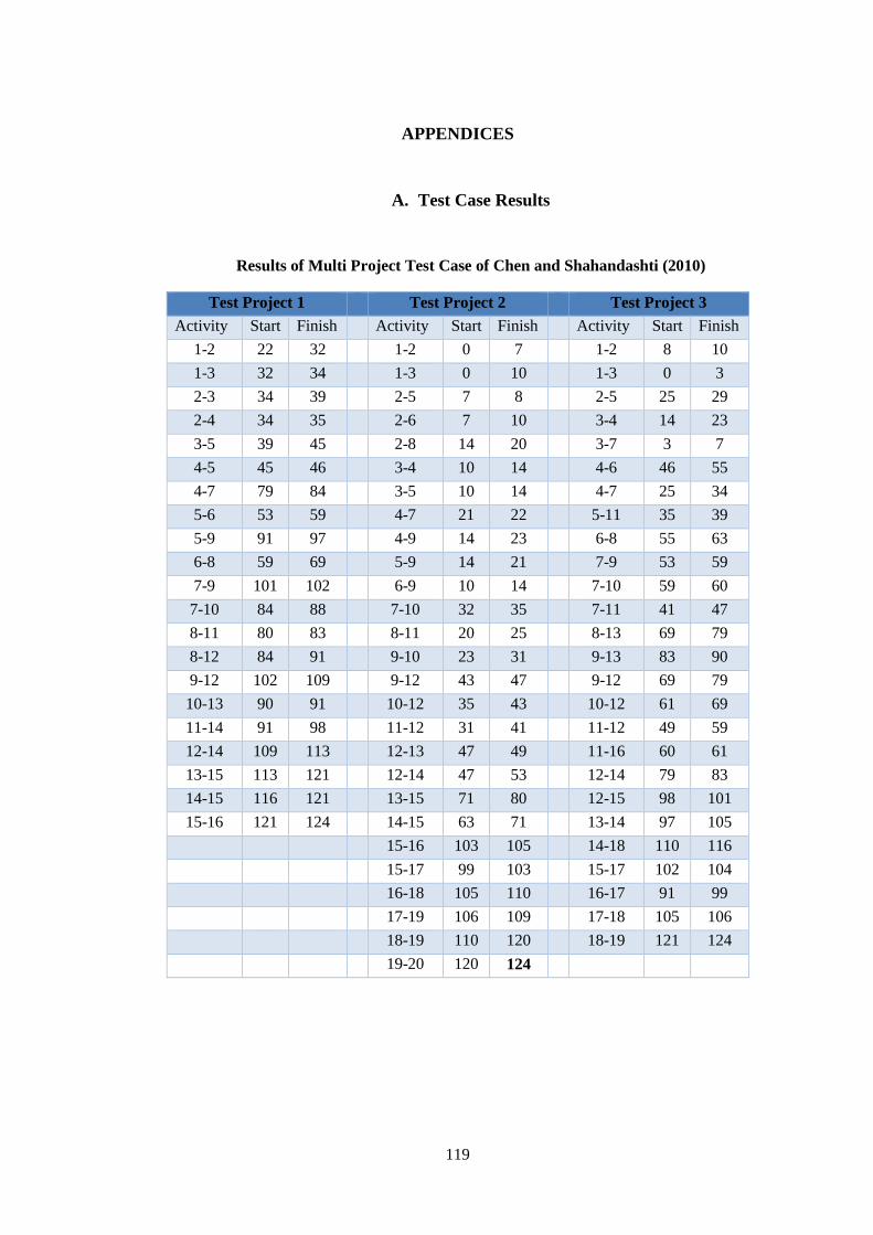
119
APPENDICES
A. Test Case Results
Results of Multi Project Test Case of Chen and Shahandashti (2010)
Test Project 1 Test Project 2 Test Project 3
Activity Start Finish Activity Start Finish Activity Start Finish
1-2 22 32 1-2 0 7 1-2 8 10
1-3 32 34 1-3 0 10 1-3 0 3
2-3 34 39 2-5 7 8 2-5 25 29
2-4 34 35 2-6 7 10 3-4 14 23
3-5 39 45 2-8 14 20 3-7 3 7
4-5 45 46 3-4 10 14 4-6 46 55
4-7 79 84 3-5 10 14 4-7 25 34
5-6 53 59 4-7 21 22 5-11 35 39
5-9 91 97 4-9 14 23 6-8 55 63
6-8 59 69 5-9 14 21 7-9 53 59
7-9 101 102 6-9 10 14 7-10 59 60
7-10 84 88 7-10 32 35 7-11 41 47
8-11 80 83 8-11 20 25 8-13 69 79
8-12 84 91 9-10 23 31 9-13 83 90
9-12 102 109 9-12 43 47 9-12 69 79
10-13 90 91 10-12 35 43 10-12 61 69
11-14 91 98 11-12 31 41 11-12 49 59
12-14 109 113 12-13 47 49 11-16 60 61
13-15 113 121 12-14 47 53 12-14 79 83
14-15 116 121 13-15 71 80 12-15 98 101
15-16 121 124 14-15 63 71 13-14 97 105
15-16 103 105 14-18 110 116
15-17 99 103 15-17 102 104
16-18 105 110 16-17 91 99
17-19 106 109 17-18 105 106
18-19 110 120 18-19 121 124
19-20 120 124
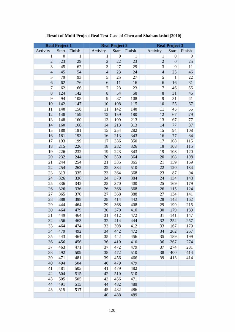
120
Result of Multi Project Real Test Case of Chen and Shahandashti (2010)
Real Project 1 Real Project 2 Real Project 3
Activity Start Finish Activity Start Finish Activity Start Finish
1 0 1 1 0 1 1 0 0
2 23 29 2 22 23 2 0 25
3 45 62 3 27 29 3 0 11
4 45 54 4 23 24 4 25 46
5 79 93 5 25 27 5 1 22
6 62 76 6 11 16 6 16 31
7 62 66 7 23 23 7 46 55
8 124 142 8 54 58 8 31 45
9 94 108 9 87 108 9 31 41
10 142 147 10 108 115 10 55 67
11 148 158 11 142 148 11 45 55
12 148 159 12 159 180 12 67 79
13 148 160 13 199 213 13 67 77
14 160 166 14 213 313 14 77 87
15 180 181 15 254 282 15 94 108
16 181 193 16 213 343 16 77 84
17 193 199 17 336 350 17 108 115
18 215 226 18 282 326 18 108 115
19 226 232 19 223 343 19 108 120
20 232 244 20 350 364 20 108 108
21 244 254 21 335 365 21 159 169
22 254 262 22 384 510 22 120 134
23 313 335 23 364 368 23 87 94
24 326 336 24 370 384 24 134 148
25 336 342 25 370 400 25 169 179
26 326 336 26 368 368 26 115 124
27 365 370 27 368 388 27 134 141
28 388 398 28 414 442 28 148 162
29 444 464 29 368 408 29 199 215
30 464 479 30 370 410 30 179 189
31 449 464 31 412 472 31 141 147
32 456 463 32 414 444 32 254 257
33 464 474 33 398 412 33 167 179
34 479 492 34 442 472 34 262 267
35 443 464 35 442 456 35 189 199
36 456 456 36 410 410 36 267 274
37 463 471 37 472 479 37 274 281
38 492 509 38 472 510 38 400 414
39 471 481 39 456 466 39 413 414
40 494 504 40 479 479
41 481 505 41 479 482
42 504 515 42 510 510
43 505 505 43 456 471
44 491 515 44 482 489
45 515 517 45 482 486
46 488 489
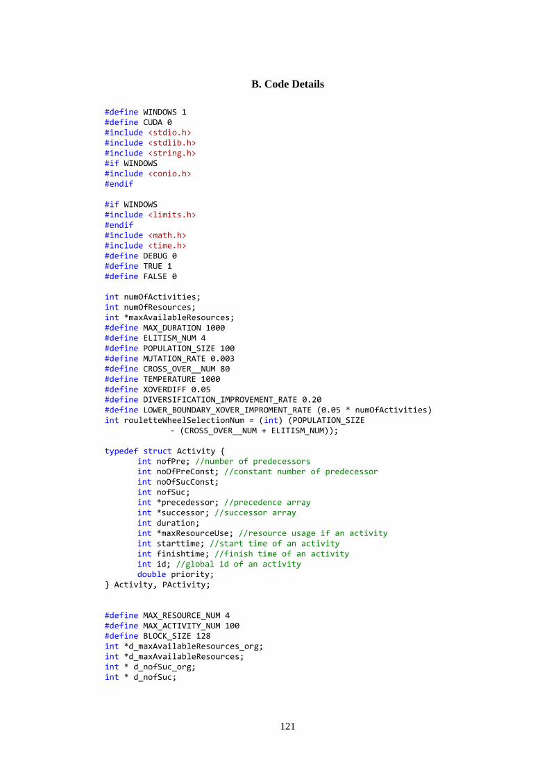
121
B. Code Details
#define WINDOWS 1 #define CUDA 0 #include <stdio.h> #include <stdlib.h> #include <string.h> #if WINDOWS #include <conio.h> #endif #if WINDOWS #include <limits.h> #endif #include <math.h> #include <time.h> #define DEBUG 0 #define TRUE 1 #define FALSE 0 int numOfActivities; int numOfResources; int *maxAvailableResources; #define MAX_DURATION 1000 #define ELITISM_NUM 4 #define POPULATION_SIZE 100 #define MUTATION_RATE 0.003 #define CROSS_OVER__NUM 80 #define TEMPERATURE 1000 #define XOVERDIFF 0.05 #define DIVERSIFICATION_IMPROVEMENT_RATE 0.20 #define LOWER_BOUNDARY_XOVER_IMPROMENT_RATE (0.05 * numOfActivities) int rouletteWheelSelectionNum = (int) (POPULATION_SIZE - (CROSS_OVER__NUM + ELITISM_NUM)); typedef struct Activity { int nofPre; //number of predecessors int noOfPreConst; //constant number of predecessor int noOfSucConst; int nofSuc; int *precedessor; //precedence array int *successor; //successor array int duration; int *maxResourceUse; //resource usage if an activity int starttime; //start time of an activity int finishtime; //finish time of an activity int id; //global id of an activity double priority; } Activity, PActivity; #define MAX_RESOURCE_NUM 4 #define MAX_ACTIVITY_NUM 100 #define BLOCK_SIZE 128 int *d_maxAvailableResources_org; int *d_maxAvailableResources; int * d_nofSuc_org; int * d_nofSuc;
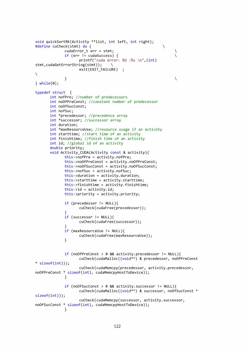
122
void quickSortRK(Activity **list, int left, int right); #define cuCheck(stmt) do { \ cudaError_t err = stmt; \ if (err != cudaSuccess) { \ printf("cuda error: %d :%s \n",(int) stmt,cudaGetErrorString(stmt)); \ exit(EXIT_FAILURE) ; \ } \ } while(0); typedef struct { int nofPre; //number of predecessors int noOfPreConst; //constant number of predecessor int noOfSucConst; int nofSuc; int *precedessor; //precedence array int *successor; //successor array int duration; int *maxResourceUse; //resource usage if an activity int starttime; //start time of an activity int finishtime; //finish time of an activity int id; //global id of an activity double priority; void Activity_CUDA(Activity const & activity){ this->nofPre = activity.nofPre; this->noOfPreConst = activity.noOfPreConst; this->noOfSucConst = activity.noOfSucConst; this->nofSuc = activity.nofSuc; this->duration = activity.duration; this->starttime = activity.starttime; this->finishtime = activity.finishtime; this->id = activity.id; this->priority = activity.priority; if (precedessor != NULL){ cuCheck(cudaFree(precedessor)); } if (successor != NULL){ cuCheck(cudaFree(successor)); } if (maxResourceUse != NULL){ cuCheck(cudaFree(maxResourceUse)); } if (noOfPreConst > 0 && activity.precedessor != NULL){ cuCheck(cudaMalloc((void**) & precedessor, noOfPreConst * sizeof(int))); cuCheck(cudaMemcpy(precedessor, activity.precedessor, noOfPreConst * sizeof(int), cudaMemcpyHostToDevice)); } if (noOfSucConst > 0 && activity.successor != NULL){ cuCheck(cudaMalloc((void**) & successor, noOfSucConst * sizeof(int))); cuCheck(cudaMemcpy(successor, activity.successor, noOfSucConst * sizeof(int), cudaMemcpyHostToDevice)); }
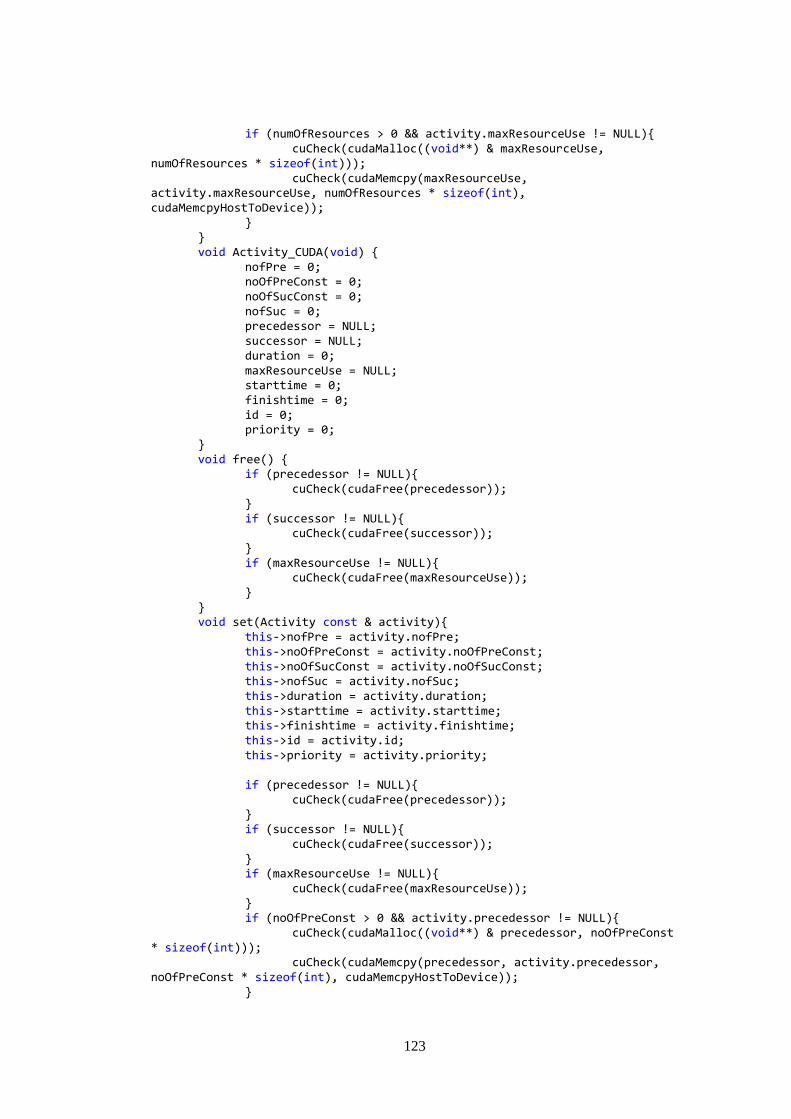
123
if (numOfResources > 0 && activity.maxResourceUse != NULL){ cuCheck(cudaMalloc((void**) & maxResourceUse, numOfResources * sizeof(int))); cuCheck(cudaMemcpy(maxResourceUse, activity.maxResourceUse, numOfResources * sizeof(int), cudaMemcpyHostToDevice)); } } void Activity_CUDA(void) { nofPre = 0; noOfPreConst = 0; noOfSucConst = 0; nofSuc = 0; precedessor = NULL; successor = NULL; duration = 0; maxResourceUse = NULL; starttime = 0; finishtime = 0; id = 0; priority = 0; } void free() { if (precedessor != NULL){ cuCheck(cudaFree(precedessor)); } if (successor != NULL){ cuCheck(cudaFree(successor)); } if (maxResourceUse != NULL){ cuCheck(cudaFree(maxResourceUse)); } } void set(Activity const & activity){ this->nofPre = activity.nofPre; this->noOfPreConst = activity.noOfPreConst; this->noOfSucConst = activity.noOfSucConst; this->nofSuc = activity.nofSuc; this->duration = activity.duration; this->starttime = activity.starttime; this->finishtime = activity.finishtime; this->id = activity.id; this->priority = activity.priority; if (precedessor != NULL){ cuCheck(cudaFree(precedessor)); } if (successor != NULL){ cuCheck(cudaFree(successor)); } if (maxResourceUse != NULL){ cuCheck(cudaFree(maxResourceUse)); } if (noOfPreConst > 0 && activity.precedessor != NULL){ cuCheck(cudaMalloc((void**) & precedessor, noOfPreConst * sizeof(int))); cuCheck(cudaMemcpy(precedessor, activity.precedessor, noOfPreConst * sizeof(int), cudaMemcpyHostToDevice)); }
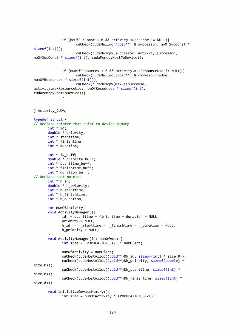
124
if (noOfSucConst > 0 && activity.successor != NULL){ cuCheck(cudaMalloc((void**) & successor, noOfSucConst * sizeof(int))); cuCheck(cudaMemcpy(successor, activity.successor, noOfSucConst * sizeof(int), cudaMemcpyHostToDevice)); } if (numOfResources > 0 && activity.maxResourceUse != NULL){ cuCheck(cudaMalloc((void**) & maxResourceUse, numOfResources * sizeof(int))); cuCheck(cudaMemcpy(maxResourceUse, activity.maxResourceUse, numOfResources * sizeof(int), cudaMemcpyHostToDevice)); } } } Activity_CUDA; typedef struct { // Declare pointer that point to device memory int * id; double * priority; int * starttime; int * finishtime; int * duration; int * id_buff; double * priority_buff; int * starttime_buff; int * finishtime_buff; int * duration_buff; // Declare host pointer int * h_id; double * h_priority; int * h_starttime; int * h_finishtime; int * h_duration; int numOfActivity; void ActivityManager(){ id = starttime = finishtime = duration = NULL; priority = NULL; h_id = h_starttime = h_finishtime = h_duration = NULL; h_priority = NULL; } void ActivityManager(int numOfAct) { int size = POPULATION_SIZE * numOfAct; numOfActivity = numOfAct; cuCheck(cudaHostAlloc((void**)&h_id, sizeof(int) * size,0)); cuCheck(cudaHostAlloc((void**)&h_priority, sizeof(double) * size,0)); cuCheck(cudaHostAlloc((void**)&h_starttime, sizeof(int) * size,0)); cuCheck(cudaHostAlloc((void**)&h_finishtime, sizeof(int) * size,0)); } void initializeDeviceMemory(){ int size = numOfActivity * (POPULATION_SIZE);
125
cuCheck(cudaMalloc((void**) & id, size * sizeof(int))); cuCheck(cudaMalloc((void**) & starttime, size * sizeof(int))); cuCheck(cudaMalloc((void**) & finishtime, size * sizeof(int))); cuCheck(cudaMalloc((void**) & priority, size * sizeof(double))); cuCheck(cudaMalloc((void**) & id_buff, size * sizeof(int))); cuCheck(cudaMalloc((void**) & starttime_buff, size * sizeof(int))); cuCheck(cudaMalloc((void**) & finishtime_buff, size * sizeof(int))); cuCheck(cudaMalloc((void**) & priority_buff, size * sizeof(double))); } void transferDataFromHostToDevice(){ int size = numOfActivity * (POPULATION_SIZE ); cuCheck(cudaMemcpy(id, h_id, size * sizeof(int), cudaMemcpyHostToDevice)); cuCheck(cudaMemcpy(starttime, h_starttime, size * sizeof(int), cudaMemcpyHostToDevice)); cuCheck(cudaMemcpy(finishtime, h_finishtime, size * sizeof(int), cudaMemcpyHostToDevice)); cuCheck(cudaMemcpy(priority, h_priority, size * sizeof(double), cudaMemcpyHostToDevice)); } void transferDataFromDeviceToHost(){ int size = numOfActivity * (POPULATION_SIZE ); cuCheck(cudaMemcpy( h_id, id,size * sizeof(int), cudaMemcpyDeviceToHost)); cuCheck(cudaMemcpy( h_starttime,starttime, size * sizeof(int), cudaMemcpyDeviceToHost)); cuCheck(cudaMemcpy( h_finishtime,finishtime, size * sizeof(int), cudaMemcpyDeviceToHost)); cuCheck(cudaMemcpy( h_priority,priority ,size * sizeof(double), cudaMemcpyDeviceToHost)); } void set(Activity *** list){ for (int i = ELITISM_NUM ; i < POPULATION_SIZE ; i ++) { quickSortRK(list[i], 0, numOfActivities - 1); } for (int i = 0; i < numOfActivity; i++) { for (int j = 0 ; j < POPULATION_SIZE; j++){ int index = i * POPULATION_SIZE + j; h_id[index] = list[j][i]->id; h_priority[index] = list[j][i]->priority; h_starttime[index] = list[j][i]->starttime; h_finishtime[index] = list[j][i]->finishtime;
126
} } } void set_back(Activity *** list){ for (int i = 0; i < numOfActivity; i++) { for (int j = 0 ; j < POPULATION_SIZE; j++){ int index = i * POPULATION_SIZE + j; list[j][i]->id = h_id[index] ; list[j][i]->priority = h_priority[index] ; list[j][i]->starttime = h_starttime[index] ; list[j][i]->finishtime = h_finishtime[index]; } } } void set_temp(Activity ** list,int i){ for (int j = 0 ; j < numOfActivity ; j++){ int index = j * POPULATION_SIZE + i; h_id[index] = list[j]->id; h_priority[index] = list[j]->priority; h_starttime[index] = list[j]->starttime; h_finishtime[index] = list[j]->finishtime; } } }ActivityManager; __global__ void solveSchedule_kernel1(int numOfResources, Activity_CUDA * temp, ActivityManager am, int *d_maxAvailableResources, int * nofSuc){ int idx = blockIdx.x * blockDim.x + threadIdx.x; if (idx < POPULATION_SIZE - ELITISM_NUM){ idx = idx + ELITISM_NUM; for (int i = am.numOfActivity - 1; i >= 0;) { for (int j = am.numOfActivity - 1; j >= 0; j--) { int jpos = j * POPULATION_SIZE + idx; if (nofSuc[am.id[jpos] * POPULATION_SIZE + idx] == 0) { am.id_buff[i * POPULATION_SIZE + idx] = am.id[jpos]; am.priority_buff[i * POPULATION_SIZE + idx] = am.priority[jpos]; i-- ; nofSuc[am.id[jpos] * POPULATION_SIZE + idx]--; for (int k = 0; k < temp[am.id[jpos]].noOfPreConst; k++) {
127
int preId = temp[am.id[jpos]].precedessor[k]; nofSuc[preId * POPULATION_SIZE + idx]--; } } } } int successerStartTime = MAX_DURATION; int dpos = (am.numOfActivity - 1) * POPULATION_SIZE + idx; am.finishtime_buff[dpos] = MAX_DURATION; am.starttime_buff[dpos]= MAX_DURATION; for (int i = am.numOfActivity - 1; i >= 0; i--) { successerStartTime = MAX_DURATION; int index = am.id_buff[i * POPULATION_SIZE +idx]; for (int k = 0; k < temp[index].noOfSucConst; k++) { int successorId = temp[index].successor[k]; int spos = temp[successorId].id * POPULATION_SIZE + idx; if (successerStartTime > am.starttime[spos]) successerStartTime = am.starttime[spos]; } int pos = index * POPULATION_SIZE + idx; am.finishtime[pos] = successerStartTime; for (int n = 0; n < numOfResources; n++) { for (int j = am.finishtime[pos]; j > am.finishtime[pos] - temp[index].duration; j--) { if (d_maxAvailableResources[n * (MAX_DURATION +1) * POPULATION_SIZE + j * POPULATION_SIZE + idx] < temp[index].maxResourceUse[n]) { am.finishtime[pos] = j - 1; n = -1; break; } } } am.starttime[pos] = am.finishtime[pos] - temp[index].duration; am.starttime_buff[i * POPULATION_SIZE + idx] = am.starttime[pos]; am.finishtime_buff[i * POPULATION_SIZE + idx] = am.finishtime[pos]; for (int e = 0; e < numOfResources; e++) { for (int k = 0; k < temp[index].duration; k++) { d_maxAvailableResources[e * (MAX_DURATION +1) * POPULATION_SIZE + (am.finishtime[index * POPULATION_SIZE + idx] - k) * POPULATION_SIZE + idx] -= temp[index].maxResourceUse[e]; }
128
} } for (int i = 0; i < am.numOfActivity; i++) { int starttime = INT_MAX; int s_id; for (int j = 0; j < am.numOfActivity; j++) { if (starttime > am.starttime_buff[j * POPULATION_SIZE + idx]) { s_id = j; starttime = am.starttime_buff[j * POPULATION_SIZE +idx]; } } int dpos = i * POPULATION_SIZE + idx; int spos = s_id * POPULATION_SIZE + idx; am.id[dpos] = am.id_buff[spos]; am.starttime[dpos] = starttime; am.finishtime[dpos] = am.finishtime_buff[spos]; am.priority[dpos] = am.priority_buff[spos]; am.starttime_buff[spos] = INT_MAX; } }// end if idx < } __global__ void solveSchedule_kernel2(int numOfResources, Activity_CUDA * temp, ActivityManager am, int *d_maxAvailableResources, int * nofSuc){ int idx = blockIdx.x * blockDim.x + threadIdx.x; if (idx < POPULATION_SIZE - ELITISM_NUM){ idx = idx + ELITISM_NUM; for (int i = 0; i < am.numOfActivity; i++) { am.starttime_buff[i * POPULATION_SIZE + idx] = 0; am.finishtime_buff[i * POPULATION_SIZE + idx] = 0; } for (int i = 0; i < am.numOfActivity; i++) { int index = am.id[i * POPULATION_SIZE + idx]; int pos = index * POPULATION_SIZE + idx; for (int k = 0; k < temp[index].noOfPreConst; k++) { int curPreId = temp[index].precedessor[k]; if (am.starttime_buff[pos] < am.finishtime_buff[curPreId * POPULATION_SIZE +idx]) { am.starttime_buff[pos] = am.finishtime_buff[curPreId * POPULATION_SIZE +idx]; } } for (int n = 0; n < numOfResources; n++) {
129
for (int j = am.starttime_buff[pos]; j < am.starttime_buff[pos] + temp[index].duration; j++) { if (d_maxAvailableResources[n * (MAX_DURATION +1) * POPULATION_SIZE + j * POPULATION_SIZE + idx] < temp[index].maxResourceUse[n]) { am.starttime_buff[pos] = j + 1; n = -1; break; } } } am.finishtime_buff[pos] = am.starttime_buff[pos] + temp[index].duration; am.starttime[i * POPULATION_SIZE + idx] = am.starttime_buff[pos]; am.finishtime[i * POPULATION_SIZE + idx] = am.finishtime_buff[pos]; for (int e = 0; e < numOfResources; e++) { for (int k = 0; k < temp[index].duration; k++) { d_maxAvailableResources[e * (MAX_DURATION +1) * POPULATION_SIZE + (am.starttime_buff[pos] + k) * POPULATION_SIZE + idx] -= temp[index].maxResourceUse[e]; } } } }// end if idx < } Activity ***geneticAlgoritm_CUDA(Activity ***list, double *preTemp, double *premotherXoverRate, double *coolingRateXover, double *coolingRate); ActivityManager * activityManager; Activity ***solutionListBeforeGeneticAlgoritm_CUDA; Activity_CUDA * dev_temp; Activity** temp; int** availabilityMatrix; int numSchedules = 500000; Activity **earlyStartLeftScheduling(Activity **solution); double getRandomNumber() { return (rand() % 10000) / (double) 10000; } Activity *createActivityPriority() { Activity *act = (Activity *) malloc(sizeof(Activity)); act->priority = getRandomNumber(); return act;
130
} void freeMemoryOfActivity(Activity *other) { free(other->maxResourceUse); free(other->precedessor); free(other->successor); } void createAvailabilityMatrix() { int k; availabilityMatrix = (int**) malloc(sizeof(int *) * numOfResources); for (k = 0; k < numOfResources; k++) { availabilityMatrix[k] = (int *) malloc(sizeof(int) * MAX_DURATION); } } void initializeAvailabilityMatrix() { int i, k; for (k = 0; k < numOfResources; k++) { for (i = 0; i < MAX_DURATION; i++) { availabilityMatrix[k][i] = maxAvailableResources[k]; } } } Activity *createActivity(Activity *other) { Activity *act = (Activity *) malloc(sizeof(Activity)); act->duration = other->duration; act->starttime = other->starttime; act->finishtime = other->finishtime; act->id = other->id; act->priority = other->priority; return act; } void calculateScheduleFromLeft(Activity **solution, int **availabilityMatrix) { int i, k, n, e, j, curPreId; Activity *cur, *pre; int startTime; for (i = 0; i < numOfActivities; i++) { temp[i]->starttime = 0; temp[i]->finishtime = 0; } for (i = 0; i < numOfActivities; i++) { cur = temp[solution[i]->id]; for (k = 0; k < cur->noOfPreConst; k++) { curPreId = cur->precedessor[k]; pre = temp[curPreId]; if (cur->starttime < pre->finishtime) { cur->starttime = pre->finishtime;
131
} } for (n = 0; n < numOfResources; n++) { for (j = cur->starttime; j < cur->starttime + cur->duration; j++) { if (availabilityMatrix[n][j] < cur->maxResourceUse[n]) { cur->starttime = j + 1; n = -1; break; } } } cur->finishtime = cur->starttime + cur->duration; startTime = cur->starttime; solution[i]->starttime = cur->starttime; solution[i]->finishtime = cur->finishtime; for (e = 0; e < numOfResources; e++) { for (k = 0; k < cur->duration; k++) { availabilityMatrix[e][startTime + k] -= cur->maxResourceUse[e]; } } } if (DEBUG) { for (i = 0; i < numOfResources; i++) { for (j = 0; j < numOfActivities; j++) { if (availabilityMatrix[i][j] < 0) { printf("as"); } } } } } Activity **scheduleFromLeft(Activity **list) { int k, i, j; Activity **scheduledChromose = (Activity**) malloc( sizeof(Activity *) * numOfActivities); for (j = 0; j < numOfActivities; j++) { temp[j]->nofPre = temp[j]->noOfPreConst; } if (DEBUG) { for (j = 0; j < numOfActivities; j++) printf("%d %d, ", temp[j]->id, temp[j]->noOfPreConst); printf("\n"); } for (i = 0; i < numOfActivities;) { for (j = numOfActivities - 1; j >= 0; j--) { if (temp[list[j]->id]->nofPre == 0) {
132
scheduledChromose[i++] = createActivity(list[j]); temp[list[j]->id]->nofPre--; for (k = 0; k < temp[list[j]->id]->noOfSucConst; k++) { int succesorId = temp[list[j]->id]->successor[k]; temp[succesorId]->nofPre--; } } } } return scheduledChromose; } void quickSortRK(Activity **list, int left, int right) { int x = left, y = right; Activity *tmp; double pivot = list[(left + right) / 2]->priority; while (x <= y) { while (list[x]->priority < pivot) x++; while (list[y]->priority > pivot) y--; if (x <= y) { tmp = list[x]; list[x] = list[y]; list[y] = tmp; x++; y--; } } if (left < y) quickSortRK(list, left, y); if (x < right) quickSortRK(list, x, right); } Activity **findRightSolution(Activity **list) { int j, i, k, preId; Activity **scheduledChromose = (Activity**) malloc( sizeof(Activity *) * numOfActivities); for (j = 0; j < numOfActivities; j++) { temp[j]->nofSuc = temp[j]->noOfSucConst; } for (i = numOfActivities - 1; i >= 0;) { for (j = numOfActivities - 1; j >= 0; j--) { if (temp[list[j]->id]->nofSuc == 0) { if (DEBUG) { printf("%d ", list[j]->id); }
133
scheduledChromose[i--] = createActivity(list[j]); temp[list[j]->id]->nofSuc--; for (k = 0; k < temp[list[j]->id]->noOfPreConst; k++) { preId = temp[list[j]->id]->precedessor[k]; temp[preId]->nofSuc--; } } } } return scheduledChromose; } void calculateRightSchedule(Activity **solution, int **availabilityMatrix) { int successerStartTime = MAX_DURATION; Activity *cur; int i, k, e, n, j, finishtime; int successorId; Activity *suc; solution[numOfActivities - 1]->finishtime = MAX_DURATION; solution[numOfActivities - 1]->starttime = MAX_DURATION; for (i = numOfActivities - 1; i >= 0; i--) { successerStartTime = MAX_DURATION; cur = temp[solution[i]->id]; for (k = 0; k < cur->noOfSucConst; k++) { successorId = cur->successor[k]; suc = temp[successorId]; if (successerStartTime > suc->starttime) successerStartTime = suc->starttime; } cur->finishtime = successerStartTime; for (n = 0; n < numOfResources; n++) { for (j = cur->finishtime; j > cur->finishtime - cur->duration; j--) { if (availabilityMatrix[n][j] < cur->maxResourceUse[n]) { cur->finishtime = j - 1; n = -1; break; } } } cur->starttime = cur->finishtime - cur->duration; finishtime = cur->finishtime; solution[i]->starttime = cur->starttime; solution[i]->finishtime = cur->finishtime; for (e = 0; e < numOfResources; e++) {
134
for (k = 0; k < cur->duration; k++) { availabilityMatrix[e][finishtime - k] -= cur->maxResourceUse[e]; } } } } Activity **earlyStartLeftScheduling(Activity **solution) { Activity **earlyLeftStartInputChromosome = (Activity**) malloc( sizeof(Activity *) * numOfActivities); Activity *activityWithSmallestStartTime = (Activity *) malloc( sizeof(Activity)); int i, j; for (i = 0; i < numOfActivities; i++) { activityWithSmallestStartTime->starttime = INT_MAX; for (j = 0; j < numOfActivities; j++) { if (activityWithSmallestStartTime->starttime > solution[j]->starttime) { activityWithSmallestStartTime = solution[j]; } } earlyLeftStartInputChromosome[i] = createActivity( activityWithSmallestStartTime); //activityWithSmallestStartTime->starttime = INT_MAX; } //free(activityWithSmallestStartTime); return earlyLeftStartInputChromosome; } void quickSortWithStartTimes(Activity **list, int left, int right) { int x = left, y = right; Activity *tmp; double pivot = list[(left + right) / 2]->starttime; while (x <= y) { while (list[x]->starttime < pivot) x++; while (list[y]->starttime > pivot) y--; if (x <= y) { tmp = list[x]; list[x] = list[y]; list[y] = tmp; x++; y--; } } if (left < y) quickSortWithStartTimes(list, left, y); if (x < right) quickSortWithStartTimes(list, x, right);
135
} void swapPriority(Activity *mother, Activity *father) { //swap function. it is used for xover double temp = mother->priority; mother->priority = father->priority; father->priority = temp; } Activity **solveSchedule(Activity **list) { int i; Activity **scheduled; Activity **earlyStartLeftScheduled; quickSortRK(list, 0, numOfActivities - 1); initializeAvailabilityMatrix(); scheduled = findRightSolution(list); calculateRightSchedule(scheduled, availabilityMatrix); earlyStartLeftScheduled = earlyStartLeftScheduling(scheduled); initializeAvailabilityMatrix(); calculateScheduleFromLeft(earlyStartLeftScheduled, availabilityMatrix); for (i = 0; i < numOfActivities; i++) { free(scheduled[i]); } free(scheduled); numSchedules--; return earlyStartLeftScheduled; } Activity **readFile(char *fileName) { int i = 0, j, k; Activity **activityList; int *numOfPres; FILE *fd = fopen(fileName, "r"); if (fd == NULL) { printf("unable to open file %s\n", fileName); exit(1); } fscanf(fd, "%d%d", &numOfActivities, &numOfResources); if (DEBUG) printf("%d %d\n", numOfActivities, numOfResources); maxAvailableResources = (int*) malloc(sizeof(int) * numOfResources); for (i = 0; i < numOfResources; i++) { fscanf(fd, "%d", &maxAvailableResources[i]); if (DEBUG) { printf("%d ", maxAvailableResources[i]); } } //printf("\n");
136
activityList = (Activity **) malloc(sizeof(Activity *) * (numOfActivities)); numOfPres = (int *) malloc(sizeof(int) * numOfActivities); for (k = 0; k < numOfActivities; k++) { numOfPres[k] = 0; } for (k = 0; k < numOfActivities; k++) { Activity *activity = createActivityPriority(); activity->id = k; activity->maxResourceUse = (int*) malloc(sizeof(int) * numOfResources); fscanf(fd, "%d", &(activity->duration)); if (DEBUG) { printf("%d ", activity->duration); } for (j = 0; j < numOfResources; j++) { fscanf(fd, "%d", &(activity->maxResourceUse[j])); if (DEBUG) printf("%d ", activity->maxResourceUse[j]); } fscanf(fd, "%d", &(activity->noOfSucConst)); activity->nofSuc = activity->noOfSucConst; if (DEBUG) printf("%d ", activity->noOfSucConst); activity->successor = (int *) malloc( sizeof(int) * activity->noOfSucConst); for (i = 0; i < activity->noOfSucConst; i++) { fscanf(fd, "%d", &(activity->successor[i])); activity->successor[i]--; numOfPres[activity->successor[i]]++; if (DEBUG) { printf("%d ", activity->successor[i]); } } //printf("---%d\n", 12); if (DEBUG) printf("\n"); activityList[k] = activity; } fclose(fd);
137
for (k = 0; k < numOfActivities; k++) { Activity *runner = activityList[k]; runner->noOfPreConst = numOfPres[k]; runner->precedessor = (int*) malloc(sizeof(int) * runner->noOfPreConst); runner->nofPre = 0; for (i = 0; i < numOfActivities; i++) { Activity * cur = activityList[i]; for (j = 0; j < cur->noOfSucConst; j++) { if (cur->successor[j] == runner->id) { runner->precedessor[runner->nofPre] = cur->id; runner->nofPre++; } } } runner->noOfPreConst = runner->nofPre; if (DEBUG) { printf("\n%d %d %d \n", runner->id, runner->nofPre, runner->noOfPreConst); for (i = 0; i < runner->nofPre; i++) printf("%d ", runner->precedessor[i]); printf("\n"); } } return activityList; } void crossOver(Activity ***solutionListBeforeGeneticAlgoritm, int motherId, int fatherId, int *curIndex, Activity ***solutionListAfterGeneticAlgoritm, double motherXoverRate) { int firstLocation = (rand() % (numOfActivities)); int secondLocation = (rand() % (numOfActivities)); int i; double diffSum; Activity **motherRow = (Activity **) malloc( sizeof(Activity*) * numOfActivities); //new chromosome Activity **fatherRow = (Activity **) malloc( sizeof(Activity*) * numOfActivities); //new chromosome Activity **mother = solutionListBeforeGeneticAlgoritm[motherId]; Activity **father = solutionListBeforeGeneticAlgoritm[fatherId]; int *choosenLocations = (int*) malloc(sizeof(int) * numOfActivities); double averageDiffSum; for (i = 0; i < numOfActivities; i++) { motherRow[i] = createActivity(mother[i]); fatherRow[i] = createActivity(father[i]); } diffSum = 0; for (i = 0; i < numOfActivities; i++) { diffSum += abs((motherRow[i]->priority - fatherRow[i]->priority)); } //cout<< "diffsum " << diffSum << "\t" << "motherXoverRate "<< motherXoverRate << endl;
138
for (i = 0; i < numOfActivities; i++) choosenLocations[i] = 0; averageDiffSum = diffSum / numOfActivities; if (averageDiffSum <= XOVERDIFF) { for (i = 0; i < (int) (motherXoverRate);) { int location = (rand() % numOfActivities); if (choosenLocations[location] == 0) { motherRow[location]->priority = getRandomNumber(); choosenLocations[location] = 1; i++; } } } if (firstLocation > secondLocation) { int temp = firstLocation; firstLocation = secondLocation; secondLocation = temp; } else if (firstLocation == secondLocation) { for (i = firstLocation; i < numOfActivities; i++) swapPriority(fatherRow[i], motherRow[i]); } else { for (i = firstLocation; i <= secondLocation; i++) { swapPriority(fatherRow[i], motherRow[i]); } } solutionListAfterGeneticAlgoritm[(*curIndex)++] = motherRow; solutionListAfterGeneticAlgoritm[(*curIndex)++] = fatherRow; free(choosenLocations); } Activity **copyChromosome(Activity **other) { Activity **chromosome = (Activity **) malloc( sizeof(Activity *) * numOfActivities); int i; for (i = 0; i < numOfActivities; i++) chromosome[i] = createActivity(other[i]); return chromosome; } void mutation(Activity ***solutionListAfterGeneticAlgoritm, double currentTemp) { int mutationIndex; int mutationGeneNum, i, finishTimeBeforeMutation, finishTimeAfterMutation; Activity **chromozomeBeforeMutation; Activity **mutationRow; Activity **chromozomeAfterMutation;
139
do { mutationIndex = (rand() % POPULATION_SIZE); } while (mutationIndex < ELITISM_NUM); chromozomeBeforeMutation = solveSchedule( solutionListAfterGeneticAlgoritm[mutationIndex]); finishTimeBeforeMutation = chromozomeBeforeMutation[numOfActivities - 1]->finishtime; mutationRow = solutionListAfterGeneticAlgoritm[mutationIndex]; mutationGeneNum = (int) ceil( POPULATION_SIZE * (numOfActivities) * MUTATION_RATE); for (i = 0; i < mutationGeneNum; i++) { int geneLocation = (rand() % (numOfActivities)); double priority = getRandomNumber(); mutationRow[geneLocation]->priority = priority; } chromozomeAfterMutation = solveSchedule(mutationRow); //chromozome has been resolved. finishTimeAfterMutation = chromozomeAfterMutation[numOfActivities - 1]->finishtime; if (finishTimeAfterMutation >= finishTimeBeforeMutation) { int delta = finishTimeAfterMutation - finishTimeBeforeMutation; double power = -(delta / (currentTemp)); double acceptancePro = exp(power); double pro = getRandomNumber(); if (acceptancePro > pro) { //rejected for (i = 0; i < numOfActivities; i++) { free(mutationRow[i]); } free(mutationRow); solutionListAfterGeneticAlgoritm[mutationIndex] = chromozomeBeforeMutation; } else { //accepted for (i = 0; i < numOfActivities; i++) { free(chromozomeBeforeMutation[i]); } free(chromozomeBeforeMutation); } } for (i = 0; i < numOfActivities; i++) { free(chromozomeAfterMutation[i]); } free(chromozomeAfterMutation);
140
} void crossOverWrapper(Activity ***solutionListBeforeGeneticAlgorithm, Activity ***solutionListAfterGeneticAlgorithm, double motherXoverRate, int *elitIndex) { int i; for (i = 0; i < CROSS_OVER__NUM / 2; i++) { int motherIndex = (rand() % POPULATION_SIZE); int fatherIndex = (rand() % POPULATION_SIZE); if (motherIndex == fatherIndex) { i--; continue; } crossOver(solutionListBeforeGeneticAlgorithm, motherIndex, fatherIndex, elitIndex, solutionListAfterGeneticAlgorithm, motherXoverRate); } } void elitism(int *elitIndex, Activity ***solutionListAfterGeneticAlgoritm, Activity ***solutionListBeforeGeneticAlgoritm) { // cout << solutionListBeforeGeneticAlgoritm[0]->solution[TOTAL_ACTIVITY - 1]->finishtime << "\n"; for (; *elitIndex < ELITISM_NUM; (*elitIndex)++) { solutionListAfterGeneticAlgoritm[(*elitIndex)] = copyChromosome( solutionListBeforeGeneticAlgoritm[(*elitIndex)]); } } void quickSortsolutionList1(Activity ***list, int left, int right) { int x = left, y = right; Activity **tmp; double pivot = list[(left + right) / 2][numOfActivities - 1]->finishtime; while (x <= y) { while (list[x][numOfActivities - 1]->finishtime < pivot) x++; while (list[y][numOfActivities - 1]->finishtime > pivot) y--; if (x <= y) { tmp = list[x]; list[x] = list[y]; list[y] = tmp; x++; y--; } } if (left < y) quickSortsolutionList1(list, left, y); if (x < right) quickSortsolutionList1(list, x, right); }
141
void rouletteWheelSelection(int *elitIndex, Activity ***solutionListAfterGeneticAlgoritm, Activity ***solutionListBeforeGeneticAlgoritm) { double selectionProbability[POPULATION_SIZE]; double sum = 0; int i, k, j; double probabilitySum = 0; for (i = 0; i < POPULATION_SIZE; i++) { sum += solutionListBeforeGeneticAlgoritm[i][numOfActivities - 1]->finishtime; } for (i = 0; i < POPULATION_SIZE; i++) selectionProbability[i] = sum / solutionListBeforeGeneticAlgoritm[i][numOfActivities - 1]->finishtime; for (i = 0; i < POPULATION_SIZE; i++) probabilitySum += selectionProbability[i]; selectionProbability[0] /= probabilitySum; for (i = 1; i < POPULATION_SIZE; i++) selectionProbability[i] = selectionProbability[i] / probabilitySum + selectionProbability[i - 1]; for (k = 0; k < rouletteWheelSelectionNum; k++) { double randNum = getRandomNumber(); for (j = 0; j < POPULATION_SIZE; j++) { if (randNum < selectionProbability[j]) { solutionListAfterGeneticAlgoritm[(*elitIndex)] = copyChromosome( solutionListBeforeGeneticAlgoritm[j]); (*elitIndex)++; break; } } } } Activity ***geneticAlgoritm(Activity ***list, double *preTemp, double *premotherXoverRate, double *coolingRateXover, double *coolingRate) { int elitIndex = 0, i, j; Activity ***solutionListBeforeGeneticAlgoritm = (Activity***) malloc( sizeof(Activity**) * POPULATION_SIZE); //Solution list is stored before GA starts Activity ***solutionListAfterGeneticAlgoritm = (Activity***) malloc( sizeof(Activity**) * POPULATION_SIZE); //Solution list is stored after GA *preTemp = *preTemp * *coolingRate;
142
if (LOWER_BOUNDARY_XOVER_IMPROMENT_RATE < *premotherXoverRate) *premotherXoverRate = *premotherXoverRate * *coolingRateXover; for (i = 0; i < ELITISM_NUM; i++) { solutionListBeforeGeneticAlgoritm[i] = copyChromosome(list[i]); } for (i = ELITISM_NUM; i < POPULATION_SIZE; i++) { solutionListBeforeGeneticAlgoritm[i] = solveSchedule(list[i]); } quickSortsolutionList1(solutionListBeforeGeneticAlgoritm, 0, POPULATION_SIZE - 1); elitism(&elitIndex, solutionListAfterGeneticAlgoritm, solutionListBeforeGeneticAlgoritm); //elitism crossOverWrapper(solutionListBeforeGeneticAlgoritm, solutionListAfterGeneticAlgoritm, *premotherXoverRate, &elitIndex); //crossover rouletteWheelSelection(&elitIndex, solutionListAfterGeneticAlgoritm, solutionListBeforeGeneticAlgoritm); //rouletwheel selection mutation(solutionListAfterGeneticAlgoritm, *preTemp); //mutation for (i = 0; i < POPULATION_SIZE; i++) { for (j = 0; j < numOfActivities; j++) { free(solutionListBeforeGeneticAlgoritm[i][j]); free(list[i][j]); } free(solutionListBeforeGeneticAlgoritm[i]); free(list[i]); } free(solutionListBeforeGeneticAlgoritm); free(list); return solutionListAfterGeneticAlgoritm; } Activity ***firstIteration(char *fileName, double *preTemp, double *coolingRate, double *coolingRateXover, double *premotherXoverRate) { int elitIndex = 0, i, j; Activity ***solutionListBeforeGeneticAlgoritm = (Activity***) malloc( sizeof(Activity**) * POPULATION_SIZE); //Solution list is stored before GA starts Activity ***solutionListAfterGeneticAlgoritm = (Activity***) malloc( sizeof(Activity**) * POPULATION_SIZE); //Solution list is stored after GA *preTemp = *preTemp * (*coolingRate); *premotherXoverRate = numOfActivities * (*coolingRateXover) * DIVERSIFICATION_IMPROVEMENT_RATE; for (i = 0; i < POPULATION_SIZE; i++) { Activity** list = readFile(fileName);
143
solutionListBeforeGeneticAlgoritm[i] = solveSchedule(list); for (j = 0; j < numOfActivities; j++) { free(list[j]); } free(list); } quickSortsolutionList1(solutionListBeforeGeneticAlgoritm, 0, POPULATION_SIZE - 1); elitism(&elitIndex, solutionListAfterGeneticAlgoritm, solutionListBeforeGeneticAlgoritm); //elitism crossOverWrapper(solutionListBeforeGeneticAlgoritm, solutionListAfterGeneticAlgoritm, *premotherXoverRate, &elitIndex); //crossover rouletteWheelSelection(&elitIndex, solutionListAfterGeneticAlgoritm, solutionListBeforeGeneticAlgoritm); //rouletwheel selection mutation(solutionListAfterGeneticAlgoritm, *preTemp); //mutation return solutionListAfterGeneticAlgoritm; } void solveProblemSet(char *fileName) { int i, j; double preTemp = TEMPERATURE; double coolingRate = 0.97; double coolingRateXover = 0.97; double premotherXoverRate; Activity ***firstGeneration; clock_t startTime; FILE *fd = fopen("out.txt", "w"); temp = readFile(fileName); srand(time(NULL)); //srand(0); createAvailabilityMatrix(); firstGeneration = firstIteration(fileName, &preTemp, &coolingRate, &coolingRateXover, &premotherXoverRate); startTime = clock(); #if CUDA Activity_CUDA * h_temp = new Activity_CUDA[numOfActivities]; for (int i = 0 ; i < numOfActivities ; i++){ h_temp[i].Activity_CUDA(); h_temp[i].set(*temp[i]); } cuCheck(cudaMalloc((void**)& dev_temp, numOfActivities * sizeof(Activity_CUDA))); cuCheck(cudaMemcpy(dev_temp, h_temp, numOfActivities * sizeof(Activity_CUDA), cudaMemcpyHostToDevice)); activityManager = (ActivityManager*) malloc(sizeof(ActivityManager)); activityManager->ActivityManager(numOfActivities); activityManager->initializeDeviceMemory();
144
int * h_maxAvailableResources; int size = numOfResources * (MAX_DURATION +1) * POPULATION_SIZE; h_maxAvailableResources = (int *) malloc(sizeof(int) * size ); for (int k = 0; k < numOfResources; k++) { for (i = 0; i <= MAX_DURATION; i++) { for (int p = 0 ; p < POPULATION_SIZE ; p++) h_maxAvailableResources[k * (MAX_DURATION + 1) * POPULATION_SIZE + i* POPULATION_SIZE + p] = maxAvailableResources[k]; } } cuCheck(cudaMalloc((void**) & d_maxAvailableResources_org, size * sizeof(int))); cuCheck(cudaMalloc((void**) & d_maxAvailableResources, size * sizeof(int))); cuCheck(cudaMemcpy( d_maxAvailableResources_org, h_maxAvailableResources,size * sizeof(int), cudaMemcpyHostToDevice)); int * h_nofSuc; h_nofSuc = (int *) malloc(sizeof(int) * numOfActivities * POPULATION_SIZE); for (int i = 0 ; i < numOfActivities ; i++) for (int p = 0 ; p < POPULATION_SIZE ; p++){ h_nofSuc[i * POPULATION_SIZE + p] = temp[i]->noOfSucConst; } cuCheck(cudaMalloc((void**) & d_nofSuc, numOfActivities * POPULATION_SIZE * sizeof(int))); cuCheck(cudaMalloc((void**) & d_nofSuc_org, numOfActivities * POPULATION_SIZE * sizeof(int))); cuCheck(cudaMemcpy( d_nofSuc_org, h_nofSuc,numOfActivities * POPULATION_SIZE * sizeof(int), cudaMemcpyHostToDevice)); #endif for (; numSchedules >= 0;) { //printf("%d\n", numSchedules); #if CUDA firstGeneration = geneticAlgoritm_CUDA(firstGeneration, &preTemp,&premotherXoverRate, &coolingRateXover, &coolingRate); #else firstGeneration = geneticAlgoritm(firstGeneration, &preTemp, &premotherXoverRate, &coolingRateXover, &coolingRate); #endif } #if CUDA for (int i = 0; i < numOfActivities; i++){ h_temp[i].free(); } free(h_temp); cuCheck(cudaFree(dev_temp)); free(h_maxAvailableResources); free(h_nofSuc);
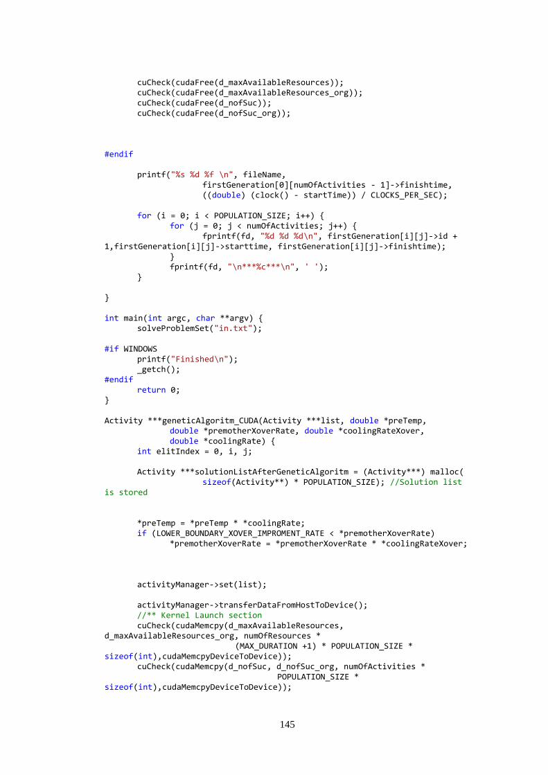
145
cuCheck(cudaFree(d_maxAvailableResources)); cuCheck(cudaFree(d_maxAvailableResources_org)); cuCheck(cudaFree(d_nofSuc)); cuCheck(cudaFree(d_nofSuc_org)); #endif printf("%s %d %f \n", fileName, firstGeneration[0][numOfActivities - 1]->finishtime, ((double) (clock() - startTime)) / CLOCKS_PER_SEC); for (i = 0; i < POPULATION_SIZE; i++) { for (j = 0; j < numOfActivities; j++) { fprintf(fd, "%d %d %d\n", firstGeneration[i][j]->id + 1,firstGeneration[i][j]->starttime, firstGeneration[i][j]->finishtime); } fprintf(fd, "\n***%c***\n", ' '); } } int main(int argc, char **argv) { solveProblemSet("in.txt"); #if WINDOWS printf("Finished\n"); _getch(); #endif return 0; } Activity ***geneticAlgoritm_CUDA(Activity ***list, double *preTemp, double *premotherXoverRate, double *coolingRateXover, double *coolingRate) { int elitIndex = 0, i, j; Activity ***solutionListAfterGeneticAlgoritm = (Activity***) malloc( sizeof(Activity**) * POPULATION_SIZE); //Solution list is stored *preTemp = *preTemp * *coolingRate; if (LOWER_BOUNDARY_XOVER_IMPROMENT_RATE < *premotherXoverRate) *premotherXoverRate = *premotherXoverRate * *coolingRateXover; activityManager->set(list); activityManager->transferDataFromHostToDevice(); //** Kernel Launch section cuCheck(cudaMemcpy(d_maxAvailableResources, d_maxAvailableResources_org, numOfResources * (MAX_DURATION +1) * POPULATION_SIZE * sizeof(int),cudaMemcpyDeviceToDevice)); cuCheck(cudaMemcpy(d_nofSuc, d_nofSuc_org, numOfActivities * POPULATION_SIZE * sizeof(int),cudaMemcpyDeviceToDevice));
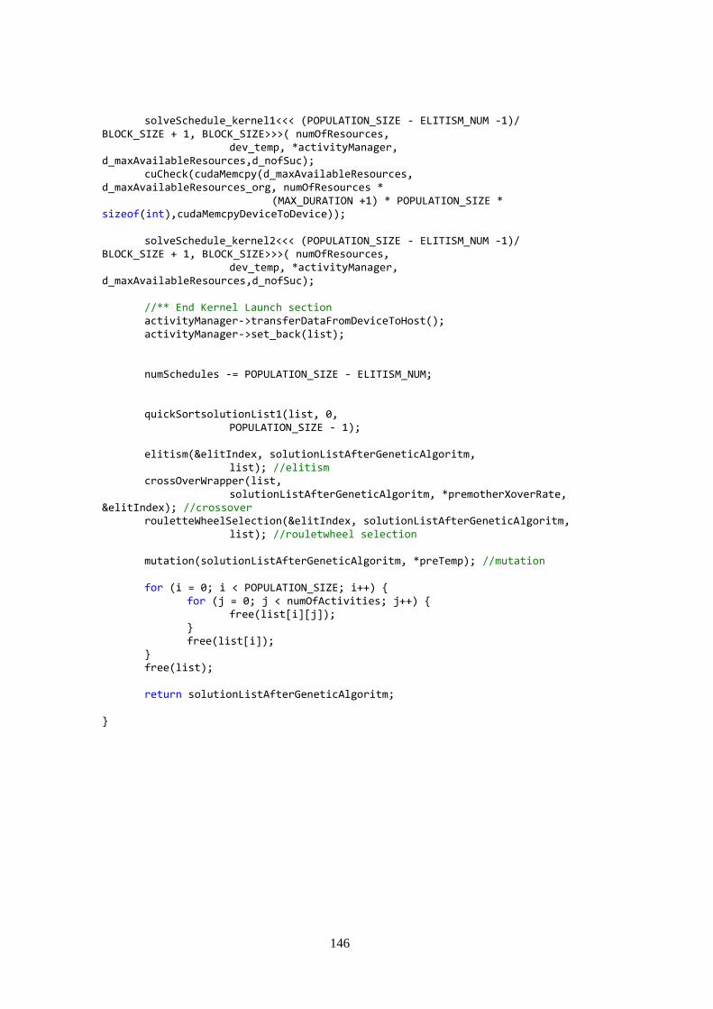
146
solveSchedule_kernel1<<< (POPULATION_SIZE - ELITISM_NUM -1)/ BLOCK_SIZE + 1, BLOCK_SIZE>>>( numOfResources, dev_temp, *activityManager, d_maxAvailableResources,d_nofSuc); cuCheck(cudaMemcpy(d_maxAvailableResources, d_maxAvailableResources_org, numOfResources * (MAX_DURATION +1) * POPULATION_SIZE * sizeof(int),cudaMemcpyDeviceToDevice)); solveSchedule_kernel2<<< (POPULATION_SIZE - ELITISM_NUM -1)/ BLOCK_SIZE + 1, BLOCK_SIZE>>>( numOfResources, dev_temp, *activityManager, d_maxAvailableResources,d_nofSuc); //** End Kernel Launch section activityManager->transferDataFromDeviceToHost(); activityManager->set_back(list); numSchedules -= POPULATION_SIZE - ELITISM_NUM; quickSortsolutionList1(list, 0, POPULATION_SIZE - 1); elitism(&elitIndex, solutionListAfterGeneticAlgoritm, list); //elitism crossOverWrapper(list, solutionListAfterGeneticAlgoritm, *premotherXoverRate, &elitIndex); //crossover rouletteWheelSelection(&elitIndex, solutionListAfterGeneticAlgoritm, list); //rouletwheel selection mutation(solutionListAfterGeneticAlgoritm, *preTemp); //mutation for (i = 0; i < POPULATION_SIZE; i++) { for (j = 0; j < numOfActivities; j++) { free(list[i][j]); } free(list[i]); } free(list); return solutionListAfterGeneticAlgoritm; }
147
C. Curriculum Vitae
Furkan UYSAL
Kalkınma Bakanlığı
Ar-Ge ve Girişimcilik Dairesi
E-postal : [email protected]
Ilgi Alanları
C ve C++ programlama ve yazilim geliştirme,
Proje yönetimi
Bilim, teknoloji ve yenilik alanında politika oluşturma
Hibe programlarının yönetimi
Teknoloji yönetimi
Eğitim
2007-2014 Orta Doğu Teknik Üniversitesi
İnşaat Mühendisliği Bölümü
Doktora Derecesi
2004-2007 Orta Doğu Teknik Üniversitesi
İnşaat Mühendisliği Bölümü
Yüksek Lisans Derecesi
2000 -2004 Orta Doğu Teknik Üniversitesi
İnşaat Mühendisliği Bölümü
Lisans Derecesi
İş Deneyimi
2012-2014 Kalkınma Bakanlığı Ar-Ge ve Girişimcilik Dairesi
Uzman
Bilim, teknoloji ve yenilik politikaları çalışmaları, Kamu Ar-
Ge yatırımlarının değerlendirilmesi,
Araştırma altyapılarına yönelik mevzuat hazırlama
çalışmaları
148
2006-2012 Türkiye Bilimsel ve Teknolojik Araştırma Kurumu
Uzman
Türkiye araştırma alanının oluşturulması (TARAL),Ulusal
hibe programlarının tasarımı, mevzuatının oluşturulması,
Araştırma projelerinin değerlendirme süreçlerinin
yönetilmesi
2004-2006 Apeas İnş., Arı Proje, Temelsu Ltd. Şti.
Teklif Mühendisi, Betonarme Tasarım Mühendisi
Başlıca Makale ve Projeler
Sertifikalar
Portland Eyalet Üniversitesi ve Portland Teknoloji Enstitüsü Teknoloji Yönetimi
Sertifikası, 2008
Kore Bilim, Teknoloji ve Gelecek Planlama Bakanlığı, INNOPOLIS Vakfı Bilim
Teknoloji Politikaları Eğitimi Sertifikası, Daejeon, Güney Kore, 2014
Sonmez R & Uysal F., (2014), A Backward-Forward Hybrid Genetic
Algorithm for Resource Constrained Multi-Project Scheduling Problem, ASCE
Journal of Computing in Civil Engineering, Doi: 10.1061/(ASCE)CP.1943-
5487.0000382
Sonmez R.& Uysal F., (2008),Geographic Information System-based
Visualization System for Planning and Monitoring of Repetitive Construction
Projects, Canadian Journal of Civil Engineering, Volume 35(11), 1342-1346
Sonmez R. & Uysal F., (2008), Planning of Linear Construction Projects Using
Geographic Information Systems, Fifth International Conference on
Construction in the 21st Century (CITC-V), İstanbul
Birden fazla projenin melez genetik algoritmalar ile çizelgelenmesi, Orta Doğu
Teknik Üniversitesi BAP Projesi (2012-2014)
Boru hattı projeleri için Coğrafi Bilgi Sistemleri (CBS) temelli planlama ve
izleme sistemi tasarımı, Orta Doğu Teknik Üniversitesi BAP Projesi (2006-
2007)