rediscovering rural appalachian communities with historical gis

southeastern geographer, 50(1) 2010: pp. 58–82

Rediscovering Rural Appalachian Communitieswith Historical GIS

GEORGE TOWERSConcord University

From the late 19th century until World War Two,

agrarian southern Appalachia was a patchwork

of small, close-knit farm communities. This his-

toric rural settlement pattern is locally recorded

in community case studies by ethnographers and

historical geographers but has not been mapped

systematically. This paper explores the hypothesis

that GIS analysis of historic topographic maps

adequately identifies the boundaries of bygone

southern Appalachian agricultural neighbor-

hoods. Using the ArcGIS cost allocation analysis

function, least cost regions are generated around

neighborhood nodes based on the energy cost of

foot travel relative to distance and slope. These

prospective agricultural neighborhoods closely

match ethnographers and historical geographers’

spatial descriptions. Mapping historic Appala-

chian agricultural neighborhoods provides an im-

portant basis for comparison with past and pres-

ent settlement patterns. The research method is

significant because it is easily replicated and may

be extended across southern Appalachia and the

past century.

Desde finales del siglo 19 hasta la Segunda

Guerra Mundial, el sur agrario de los Apalaches

era un mosaico de comunidades agrícolas pe-

queñas y muy unidas. Este patrón histórico de

asentamiento rural es registrado a nivel local en

estudios de etnógrafos y geógrafos históricos sobre

casos comunitarios, sinembargo no ha sido car-

tografiada de forma sistemática. Este trabajo ex-

plora la hipótesis de que el análisis mapas to-

pográficos históricos utilizando SIG identifica ad-

ecuadamente los límites pasados de los barrios

agrícolas del sur de los Apalaches. Utilizando la

función de análisis de asignación de costos de

ArcGIS, regiones de menor costo son generadas

alrededor de los nodos de los barrios, basadas en

el costo de la energía de viajes a pie con respecto a

distancia y pendiente. Estos vecindarios agrícolas

prospectos se asemejan a las descripciones espa-

ciales de los etnógrafos y los geógrafos históricos.

Cartografiar barrios agrícolas históricos en los

Apalaches provee una importante base para la

comparación de pasados y presentes patrones de

asentamiento. Este método de investigación es sig-

nificativo porque es fácilmente replicable y puede

ser empleado a través de los Apalaches del Sur y

del siglo pasado.

key words: historical GIS, Appalachia,

agricultural neighborhoods, topographic maps,

West Virginia, landscape, social history,

farming

introduction

This research assesses the hypothesisthat historical GIS (HGIS) may be used tomap an extinct and iconic American land-scape: the southern Appalachian agricul-tural neighborhoods of a century ago.HGIS enables researchers to ask geograph-ical questions of history and supportsits answers with maps and spatial analy-

Rediscovering Rural Appalachian Communities 59

sis. Over the last two decades, HGIS hasevolved from a research method to a well-recognized interdisciplinary field of study(Baker 2003; Colten et al. 2005; Gregoryand Healey 2007; Knowles 2008).

Occupying five or six square kilometerseach, agricultural neighborhoods of a fewdozen farm families ordered southern Ap-palachia’s rural social landscape.

‘‘Preindustrial mountain society hadbeen based upon a system of small, in-dependent family farms, clustered to-gether in diffuse open-countryneighborhoods’’ (Eller 1982, p 194).

Neighborhoods, according to James S.Brown, a leader in mid-20th century south-ern Appalachian ethnography, are definedby social solidarity, interdependence, anda shared community of interests (1988).Throughout the region, anthropologistsand sociologists reported that neighbor-hood solidarity was cemented throughfamily ties and Protestant fundamentalismwhile subsistence agriculture engenderedthe neighborly interdependence that fos-tered a community of interests (Pearsall1959; Stephenson 1968; Kaplan 1971;Beaver 1976; Photiadis 1980; Martin1984). Ethnographers’ emphasis on socialorganization led them to the label ‘‘kinshipneighborhoods.’’ The current research,however, focuses on the cultural land-scape and will instead use the term ‘‘agri-cultural neighborhoods’’ to distinguishthis settlement pattern from other re-gional rural communities like hamlets andcoal camps while retaining an emphasis onlocal social integration.

Agricultural neighborhoods were apassing phenomena, existing between theCivil War and World War Two. Previously,agricultural communities spread them-

selves over much more territory. For exam-ple, early 19th century farm neighborhoodsin Tazewell County, Virginia of 25 to 30households took up 25 to 65 square kilo-meters (Mann 1995). By the late 1800s,the labor demands of low technology sub-sistence agriculture had sustained popula-tion growth sufficient to crowd the coun-tryside (Salstrom 1994; Billings and Blee2000). Farms were subdivided among fam-ily members. For instance, a re-visitation ofeastern Kentucky’s ‘‘Beech Creek’’ neigh-borhood found that the three farms in thearea in 1850 had multiplied more than ten-fold by 1942 (Billings and Blee 2000). Ag-riculture also expanded to exhaust arableland. Martin (1984) provides a case studyof this process in his description of Ken-tucky farmers bringing the isolated Headof Hollybush Hollow into agricultural pro-duction in the early 1880s.

Coexisting with encroaching coal campsin the first decades of the last century,farm neighborhoods emptied out in the1940s and 1950s. Farmers and their chil-dren found factory jobs and the Great So-ciety of the 1960s declared war on the ves-tigial Appalachian culture of poverty (Eller2008). A primarily residential presence—rural sprawl—has since settled over theold landscape of agricultural production.Invaded, abandoned, and obscured, thetraditional agricultural neighborhoodhas ‘‘disappeared from the map’’ (Howell2003, p 122).

A case study of Summers County, WestVirginia assesses the hypothesis that HGISmay identify the boundaries of historicsouthern Appalachian agricultural neigh-borhoods (see Figure 1). The primary datafor this study are century-old 1:62,500scale U.S. Geological Survey (USGS) to-pographic maps covering 15 minute quad-

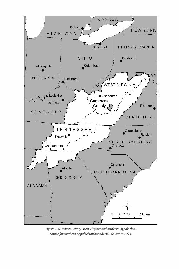
Figure 1. Summers County, West Virginia and southern Appalachia.

Source for southern Appalachian boundaries: Salstrom 1994.


rangles of latitude and longitude. HGISmethods are used to convert territory sur-rounding neighborhood nodes—the coun-try schools and hamlet centers shown onthe historic topographic maps—into po-tential agricultural neighborhoods. HGISanalysis compares the spatial arrange-ment of the houses, country schools, andchurches in the prospective agriculturalneighborhoods with the consistent neigh-borhood settlement patterns described inethnographic case studies made acrosssouthern Appalachia. If corroborated byevidence from ethnography and historicalquantitative data, the HGIS methodologymay be extended across the southern Ap-palachian region. Subsequent researchmay lead to construction of regional set-tlement pattern datasets for comparativetemporal and spatial analysis.

study area

The Summers County portions of the1912 Big Bend and Meadow Creek 15minute USGS quadrangles serve as thestudy area for historical and geographicalreasons (see Figure 2). Historically, thesequads were the first mapped in the Ap-palachian plateau of southern West Vir-ginia. They have been recently scannedand georeferenced by the West VirginiaDepartment of Environmental Protectionand the West Virginia GIS Technical Cen-ter (Dawson et al. 2007).

Dominating the rural landscape de-picted on the Big Bend and Meadow Creekmaps were diversified family farms. Whilecorn occupied half of the cultivated acre-age, farmers also grew wheat, oats, andhay and tended vegetable gardens andfruit trees. Livestock included milk cows,hogs and sheep (Unrau 1996). The farm

population of 11,008 was 82 percent ofthe county’s rural total and 84 percent ofrural dwellings were farmhouses. In For-est Hill, Jumping Branch, and Pipestem,the three rural southern magisterial dis-tricts without the railroad and without siz-able unincorporated villages, more than90 percent of people lived on farms (U.S.Census 1913).

HGIS allows local case studies to be in-tegrated with regional scale investigation,offering the opportunity to assess whetherSummers County is representative of late19th and early 20th century agriculturalsouthern Appalachia. Cunfer (2005) pro-vides an example of this approach by sup-porting his localized longitudinal casestudies of farming practices on the GreatPlains with a region-wide HGIS datasetderived from agricultural censuses. Theregional boundaries shown in Figure 1have found general agreement among his-torians of southern Appalachia (Salstrom1994; Williams 2001) and are the basis fora county level HGIS dataset developedfrom decadal census data that ranges from1880 through 1940 and speaks to farmsize and farm density. Variables includethe number of acres per farm, the numberof farms per square mile, the percent ofcounty land in farms, the growth rate offarms, and the rate of change in averagefarm size.

For each southern Appalachian county,these variables were standardized with zscores (see Tables 1 and 2). This resultedin seven z scores for the farm size and thetwo farm density measures and six z scoresfor the two rate of change variables. Theabsolute values of z scores in each cate-gory were then averaged to create a singlecomparative index of each county’s corre-spondence to regional norms. By this mea-

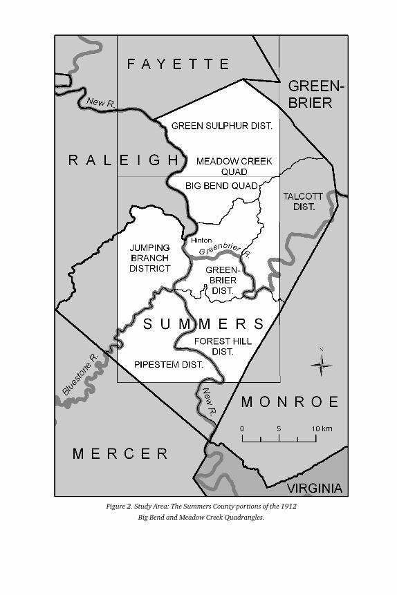
Figure 2. Study Area: The Summers County portions of the 1912

Big Bend and Meadow Creek Quadrangles.


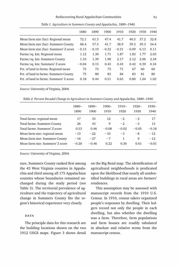
Table 1. Agriculture in Summers County and Appalachia, 1880–1940.

1880 1890 1900 1910 1920 1930 1940

Mean farm size (ha): Regional mean 72.1 61.5 47.4 41.7 40.5 37.2 32.8

Mean farm size (ha): Summers County 68.4 57.5 41.7 38.9 39.3 39.3 34.4

Mean farm size (ha): Summers’ Z score –0.13 –0.19 –0.32 –0.21 –0.09 0.13 0.11

Farms/sq. km: Regional mean 1.12 1.30 1.71 1.87 1.83 1.77 2.03

Farms/sq. km: Summers County 1.10 1.39 1.98 2.17 2.12 2.06 2.34

Farms/sq. km: Summers’ Z score –0.04 0.15 0.43 0.43 0.42 0.39 0.34

Pct. of land in farms: Regional mean 72 72 73 71 67 60 60

Pct. of land in farms: Summers County 75 80 83 84 83 81 80

Pct. of land in farms: Summers’ Z score 0.18 0.44 0.51 0.65 0.80 1.04 1.02

Source: University of Virginia, 2004.

Table 2. Percent Decadal Change in Agriculture in Summers County and Appalachia, 1880–1940.

1880–

1890

1890–

1900

1900–

1910

1910–

1920

1920–

1930

1930–

1940

Total farms: regional mean 17 33 12 –2 –2 17

Total farms: Summers County 26 43 9 –2 –3 13

Total farms: Summers’ Z score 0.53 0.46 –0.08 –0.02 –0.05 –0.18

Mean farm size: regional mean –13 –22 –10 –3 –8 –12

Mean farm size: Summers County –16 –27 –7 1 0 –12

Mean farm size: Summers’ Z score –0.20 –0.46 0.22 0.36 0.61 –0.01


sure, Summers County ranked first amongthe 43 West Virginia counties in Appala-chia and third among all 175 Appalachiancounties whose boundaries remained un-changed during the study period (seeTable 3). The territorial prevalence of ag-riculture and the trajectory of agriculturalchange in Summers County fits the re-gion’s historical experience very closely.

data

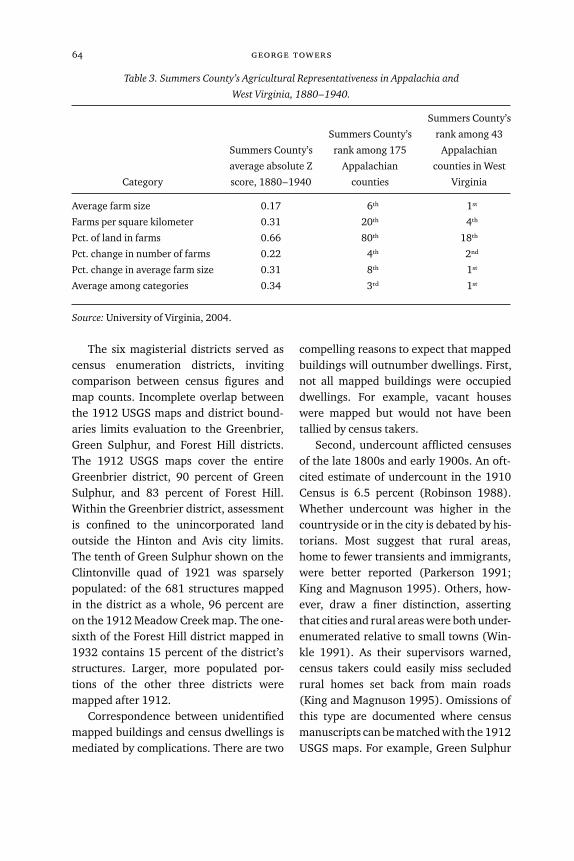
The principle data for this research arethe building locations shown on the two1912 USGS maps. Figure 3 shows detail

on the Big Bend map. The identification ofagricultural neighborhoods is predicatedupon the likelihood that nearly all uniden-tified buildings in rural areas are farmers’residences.

This assumption may be assessed withmanuscript records from the 1910 U.S.Census. In 1910, census takers organizedpeople’s responses by dwelling. Their led-gers record not only the people in eachdwelling, but also whether the dwellingwas a farm. Therefore, farm populationsand farm houses are readily tabulatedin absolute and relative terms from themanuscript census.

64 george towers

Table 3. Summers County’s Agricultural Representativeness in Appalachia and

West Virginia, 1880–1940.

Category

Summers County’s

average absolute Z

score, 1880–1940

Summers County’s

rank among 175

Appalachian

counties

Summers County’s

rank among 43

Appalachian

counties in West

Virginia

Average farm size 0.17 6th 1st

Farms per square kilometer 0.31 20th 4th

Pct. of land in farms 0.66 80th 18th

Pct. change in number of farms 0.22 4th 2nd

Pct. change in average farm size 0.31 8th 1st

Average among categories 0.34 3rd 1st


The six magisterial districts served ascensus enumeration districts, invitingcomparison between census figures andmap counts. Incomplete overlap betweenthe 1912 USGS maps and district bound-aries limits evaluation to the Greenbrier,Green Sulphur, and Forest Hill districts.The 1912 USGS maps cover the entireGreenbrier district, 90 percent of GreenSulphur, and 83 percent of Forest Hill.Within the Greenbrier district, assessmentis confined to the unincorporated landoutside the Hinton and Avis city limits.The tenth of Green Sulphur shown on theClintonville quad of 1921 was sparselypopulated: of the 681 structures mappedin the district as a whole, 96 percent areon the 1912 Meadow Creek map. The one-sixth of the Forest Hill district mapped in1932 contains 15 percent of the district’sstructures. Larger, more populated por-tions of the other three districts weremapped after 1912.

Correspondence between unidentifiedmapped buildings and census dwellings ismediated by complications. There are two

compelling reasons to expect that mappedbuildings will outnumber dwellings. First,not all mapped buildings were occupieddwellings. For example, vacant houseswere mapped but would not have beentallied by census takers.

Second, undercount afflicted censusesof the late 1800s and early 1900s. An oft-cited estimate of undercount in the 1910Census is 6.5 percent (Robinson 1988).Whether undercount was higher in thecountryside or in the city is debated by his-torians. Most suggest that rural areas,home to fewer transients and immigrants,were better reported (Parkerson 1991;King and Magnuson 1995). Others, how-ever, draw a finer distinction, assertingthat cities and rural areas were both under-enumerated relative to small towns (Win-kle 1991). As their supervisors warned,census takers could easily miss secludedrural homes set back from main roads(King and Magnuson 1995). Omissions ofthis type are documented where censusmanuscripts can be matched with the 1912USGS maps. For example, Green Sulphur

Figure 3. Detail view of the area around the Low Gap School on the 1912 Big Bend Quadrangle.

66 george towers

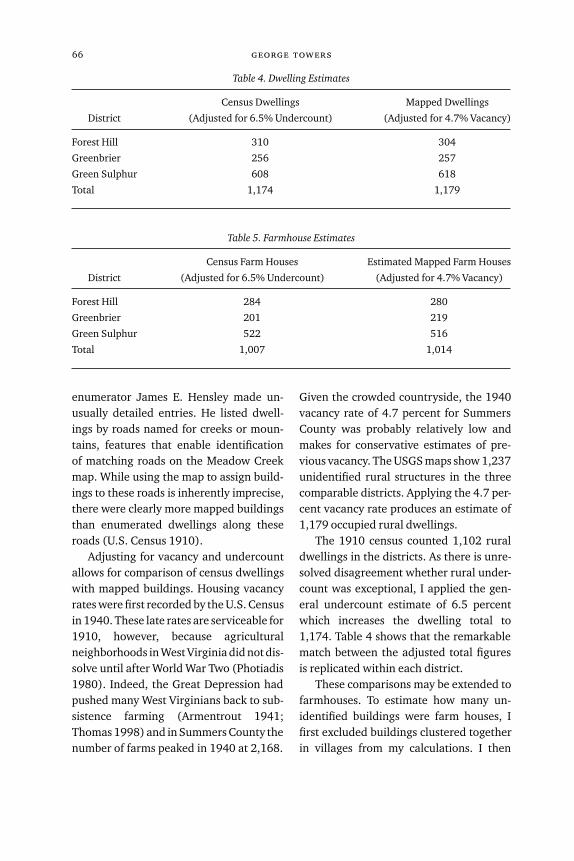
Table 4. Dwelling Estimates

District

Census Dwellings

(Adjusted for 6.5% Undercount)

Mapped Dwellings

(Adjusted for 4.7% Vacancy)

Forest Hill 310 304

Greenbrier 256 257

Green Sulphur 608 618

Total 1,174 1,179

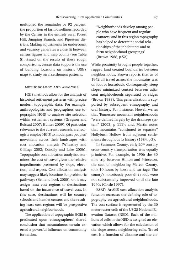
Table 5. Farmhouse Estimates

District

Census Farm Houses

(Adjusted for 6.5% Undercount)

Estimated Mapped Farm Houses

(Adjusted for 4.7% Vacancy)

Forest Hill 284 280

Greenbrier 201 219

Green Sulphur 522 516

Total 1,007 1,014

enumerator James E. Hensley made un-usually detailed entries. He listed dwell-ings by roads named for creeks or moun-tains, features that enable identificationof matching roads on the Meadow Creekmap. While using the map to assign build-ings to these roads is inherently imprecise,there were clearly more mapped buildingsthan enumerated dwellings along theseroads (U.S. Census 1910).

Adjusting for vacancy and undercountallows for comparison of census dwellingswith mapped buildings. Housing vacancyrates were first recorded by the U.S. Censusin 1940. These late rates are serviceable for1910, however, because agriculturalneighborhoods in West Virginia did not dis-solve until after World War Two (Photiadis1980). Indeed, the Great Depression hadpushed many West Virginians back to sub-sistence farming (Armentrout 1941;Thomas 1998) and in Summers County thenumber of farms peaked in 1940 at 2,168.

Given the crowded countryside, the 1940vacancy rate of 4.7 percent for SummersCounty was probably relatively low andmakes for conservative estimates of pre-vious vacancy. The USGS maps show 1,237unidentified rural structures in the threecomparable districts. Applying the 4.7 per-cent vacancy rate produces an estimate of1,179 occupied rural dwellings.

The 1910 census counted 1,102 ruraldwellings in the districts. As there is unre-solved disagreement whether rural under-count was exceptional, I applied the gen-eral undercount estimate of 6.5 percentwhich increases the dwelling total to1,174. Table 4 shows that the remarkablematch between the adjusted total figuresis replicated within each district.

These comparisons may be extended tofarmhouses. To estimate how many un-identified buildings were farm houses, Ifirst excluded buildings clustered togetherin villages from my calculations. I then


multiplied the remainder by 92 percent,the proportion of farm dwellings recordedby the Census in the entirely rural ForestHill, Jumping Branch, and Pipestem dis-tricts. Making adjustments for undercountand vacancy generates a close fit betweencensus figures and map counts (see Table5). Based on the results of these roughcomparisons, census data supports the useof building locations on historic USGSmaps to study rural settlement patterns.

methodology and analysis

HGIS methods allow for the analysis ofhistorical settlement patterns with precisemodern topographic data. For example,anthropologists and geographers use to-pographic HGIS to analyze site selectionwithin settlement systems (Gragson andBolstad 2007; Hunter 2009). Of particularrelevance to the current research, archeol-ogists employ HGIS to model past peoples’movement across their landscapes withcost allocation analysis (Wheatley andGillings 2002; Conolly and Lake 2006).Topographic cost allocation analysis deter-mines the cost of travel given the relativeimpediments presented by slope, eleva-tion, and aspect. Cost allocation analysismay suggest likely locations for prehistoricpathways (Bell and Lock 2000), or, it mayassign least cost regions to destinationsbased on the incurrence of travel cost. Inthis case, destinations will be countryschools and hamlet centers and the result-ing least cost regions will be prospectiveagricultural neighborhoods.

The application of topographic HGIS ispredicated upon ethnographers’ sharedconclusion that mountainous terrain ex-erted a powerful influence on communityformation.

‘‘Neighborhoods develop among peo-ple who have frequent and regularcontacts, and in this region topographyhas helped to determine social rela-tionships of the inhabitants and toform neighborhood groupings’’(Brown 1988, p 52).

While proximity brought people together,rugged land created boundaries betweenneighborhoods. Brown reports that as of1942 all travel across the mountains wason foot or horseback. Consequently, steepslopes minimized contact between adja-cent neighborhoods separated by ridges(Brown 1988). This generalization is sup-ported by subsequent ethnography andoral history. For instance, Howell writesthat Tennessee mountain neighborhoods‘‘were defined largely by the drainage sys-tem’’ (2003, p 111); and, Martin notesthat mountains ‘‘continued to separate’’Hollybush Hollow from adjacent settle-ments throughout its history (1984, p 3).

In Summers County, early 20th centurycross-country transportation was equallyprimitive. For example, in 1906 the 30mile trip between Hinton and Princeton,the seat of neighboring Mercer County,took 10 hours by horse and carriage. Thecounty’s notoriously poor dirt roads werenot substantially improved until the late1940s (Cottle 1997).

ESRI’s ArcGIS cost allocation analysisfunction recreates the defining role of to-pography on agricultural neighborhoods.The cost surface is represented by the 30meter raster cells of the USGS National El-evation Dataset (NED). Each of the mil-lions of cells in the NED is assigned an ele-vation which allows for the calculation ofthe slope across neighboring cells. Travelcost is a function of distance and the en-

68 george towers

ergy cost of walking at slope. For each des-tination cell representing a country schoolor a hamlet center, a region is generatedfrom the surrounding cells for which thetravel cost to that destination is the least.Hypothetically, these least cost regions ap-proximate the boundaries of the southernAppalachian agricultural neighborhoodsof a hundred years ago.

Hamlet centers and country schoolsare destinations. Hamlets offered essentialcommercial and social services to the sur-rounding countryside. For example, a typi-cal early 20th Century hamlet of 100 peo-ple may have had a post office, a church, agrocery store, a feed store, a mill, and aschool (Hart 1975). Assuming an averagehousehold size of five or six, a dozen ortwo houses would have complemented thehandful of community and commercialbuildings. Hamlets were named on the1912 USGS maps. A central point withineach of the study area’s 36 named ham-lets was digitized with ArcGIS. Consistentwith the premise that these were small ser-vice centers, 33 of the 36 hamlets had postoffices in 1912 and two of the other threehad post offices that were closed before1912 (Helbock 2004).

Within the study area, the cluster ofsome twenty structures at Green SulphurSprings is a representative hamlet. Farmfamilies from the surrounding area regu-larly traveled to Green Sulphur Springs totrade at the store and attend church (New-comb 2008). Smaller hamlets in the studyarea also served as central places and shiftsize expectations downward. For example,True, which lay at the confluence of theBluestone and New Rivers until it wasflooded by the construction of the Blue-stone Dam in 1948, was a tiny hamlet of-fering commercial services and river ac-

cess to communities up Pipestem Creekand on adjacent Tallery Mountain. Onehundred years ago, True ran a kilometeror two along the south bank of the Blue-stone. Only five structures, however, in-cluding a mill, store and post office,formed the hamlet at the mouth of Pipe-stem Creek. Four additional structures,presumably farmhouses, were locatedalong the floodplain in the True vicin-ity (Summers County Historical Society1984; Sanders 1992). Similarly, Warfordwas a New River hamlet comprised of afour building cluster that included a coun-try store, post office, and a blacksmithshop (Sanders 1992). Like True, a halfdozen residences were scattered throughthe surrounding neighborhood.

Country schools were community nodesfor the agricultural neighborhoods thatfilled the countryside between hamlets.Agricultural neighborhoods, as discussedabove, were small kinship-based commu-nities. A representative example from thestudy area is the River Ridge neighbor-hood. River Ridge rises sharply betweenPipestem Creek and the New River. TheLane, Keaton, Farley, and Pettrey familiesestablished a tightly knit neighborhood onthe ridge in the early 1800s after valleyland was taken. The population pressurerepresentative of the region certainly ap-plied to River Ridge: an early family ofLanes included 15 children and a late 19th

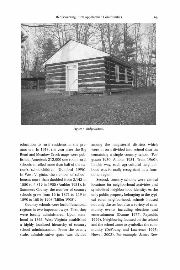
century Keaton fathered a dozen with twowives. Community buildings, Ridge School(see Figure 4) and a log church, werebuilt in the 1870s in a central location(Summers County Historical Society 1984;Sanders 1992).

Peaking in the first decades of the lastcentury, country schools were an expedi-ent means of providing mandated public


Figure 4. Ridge School.

education to rural residents in the pre-auto era. In 1913, the year after the BigBend and Meadow Creek maps were pub-lished, America’s 212,000 one room ruralschools enrolled more than half of the na-tion’s schoolchildren (Gulliford 1996).In West Virginia, the number of school-houses more than doubled from 2,142 in1880 to 4,819 in 1905 (Ambler 1951). InSummers County, the number of countryschools grew from 16 in 1871 to 119 in1890 to 160 by 1908 (Miller 1908).

Country schools were loci of functionalregions in two important ways. First, theywere locally administered. Upon state-hood in 1863, West Virginia establisheda highly localized hierarchy of countryschool administration. From the countyscale, administrative space was divided

among the magisterial districts whichwere in turn divided into school districtscontaining a single country school (Fer-guson 1950; Ambler 1951; Trent 1960).In this way, each agricultural neighbor-hood was formally recognized as a func-tional region.

Second, country schools were centrallocations for neighborhood activities andsymbolized neighborhood identity. As theonly public property belonging to the typi-cal rural neighborhood, schools housednot only classes but also a variety of com-munity events including elections andentertainment (Dunne 1977; Reynolds1999). Neighboring focused on the schooland the school came to symbolize the com-munity (DeYoung and Lawrence 1995;Howell 2003). For example, James New

70 george towers

comb, who attended Summers County’sRed Spring country school in the 1920s,vividly recalls the pie suppers and cake-walks that gathered his neighbors atthe school on Friday evenings (Newcomb2008). In short, ‘‘The schools housed theactivities that joined people into a com-munity, and the identity of rural com-munities became inextricably linked withtheir schools’’ (Gulliford 1996, p 35).

Consistent with their function as com-munity centers and in order to minimizechildren’s walk to class, schools were cen-trally located within agricultural neigh-borhoods. Anecdotally, Newcomb relatesthat the Red Spring School was sited sothat community members were no morethan a mile (1.6 km) walk from the school(2008). A 1929 West Virginia Departmentof Education survey of 29 rural school dis-tricts, including one in Summers County,found that in almost two-thirds of the dis-tricts, more than 70 percent of studentslived within 1.6 kilometers of their school.Conversely, in 87 percent of the districts,less than 20 percent of students lived morethan 2.4 kilometers from school (Holy1929). Centrally located and regularly dis-tributed, country school locations com-prise a spatial catalog of functional nodesrequired for the GIS analysis. The 74schools located in the countryside awayfrom named places serve as potentialneighborhood nodes.

Country churches also organized agri-cultural neighborhoods. Ethnographersattest that neighborhood churches werean important element of community or-ganization (Stephenson 1968; Photiadis1980). In some neighborhoods, congrega-tions met in schoolhouses (Brown 1988);in others, freestanding churches occu-pied central community locations (Beaver

1976). Twenty-five churches appear onthe USGS maps in the study area. Of these,22 are in hamlets or near a school andwere not considered as unique nodes.Three churches, however, were aloneamidst linear settlement patterns alongstreams and were included as destinationsin the cost allocation analysis.

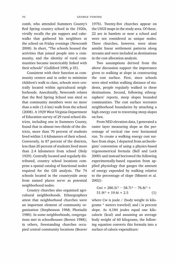
Two assumptions derived from theabove discussion support the importancegiven to walking at slope in constructingthe cost surface. First, since schoolswere sited within walking distance of stu-dents, people regularly walked to thesedestinations. Second, following ethnog-raphers’ reports, steep slopes boundedcommunities. The cost surface recreatesneighborhood boundaries by attaching ahigh energy cost to traversing steep slopeson foot.

From NED elevation data, I generated araster layer measuring slope as the per-centage of vertical rise over horizontalrun. To create a walking energy cost sur-face from slope, I departed from archeolo-gists’ convention of using a physics-basedtrigonometrical formula (Bell and Lock2000) and instead borrowed the followingexperimentally-based equation from ap-plied physiology that gauges the amountof energy expended by walking relativeto the percentage of slope (Minetti et al.2002):

Cwi = 280.5i 5 – 58.7i 4 – 76.8i 3 +51.9i 2 + 19.6i + 2.5 (1)

where Cw is joule / (body weight in kilo-grams * meters traveled) and i is percentslope. As 4,184 joules equal one kilo-calorie (kcal) and assuming an averagebody weight of 60 kilograms, the follow-ing equation converts this formula into asurface of caloric expenditure:


kcal = (Cwi * 60 * meters traveled) /4184 (2)

The cost surface was modified to allow thestudy area’s three swift rivers to boundneighborhoods. Sections of the Bluestone,Greenbrier, and New that were mapped astwo dimensional features on the 1912 to-pographic maps were digitized as poly-gons interrupted at bridge locations. As-signing the rivers an insurmountably highvalue of 100,000 calories turned the riverpolygons into neighborhood barriers.

Figures 3 and 5 show how the analy-sis converts topography to least cost zones.Figure 3 is the portion of the 1912 BigBend Quadrangle immediately surround-ing a node, Low Gap School. Figure 5 over-lays the semi-transparent cost surfaceon the topographic map and shows theboundaries (in white) of the Low GapSchool least cost zone. As darker shadesindicate greater cost, Figure 5 shows howslopes impart higher travel cost and howzone boundaries tend to follow high-coststeep slopes. The overlay suggests thatLow Gap School, at a low spot, or ‘‘gap’’along Wolf Creek Mountain (the letters‘‘WOLF CR’’ are splined to follow the ridge-line on the map), was the focal point for aridgetop agricultural neighborhood. Thecost allocation analysis generated an ini-tial least cost rural zone around each ofthe 111 country schools, hamlet centers,and country churches that were digitizedas point features. Of these, 32 were trun-cated by the study area boundaries andwere removed from further analysis. Ofthe remaining 79, 24 are hamlets orga-nized around hamlet centers; the 53 cen-tered on country schools and the 2 basedon churches are presumed to be agricul-tural neighborhoods.

results and discussion

The following discussion of these zones’spatial qualities is based on the precedingdemonstration that agricultural neighbor-hoods in Summers County are representa-tive of those throughout southern Appala-chia. As presented above, anthropologistsand sociologists found great commonal-ity amongst agricultural neighborhoodsacross the region and local histories ofcommunities like River Ridge match ex-pectations from ethnography. The preced-ing census data analysis provides quan-titative evidence that Summers Countyagriculture was emblematic of the region.With the establishment of the study area’srepresentativeness, the hypothesis thatHGIS analysis reveals the boundaries ofhistoric southern Appalachian agriculturalneighborhoods may be examined.

I compared the zones’ spatial charac-teristics—building counts, geographicsize, and building density—with those re-ported for southern Appalachian agri-cultural neighborhoods by ethnographersand historical geographers. Ethnogra-phers’ estimates of residences per south-ern Appalachian agricultural neighbor-hood range from 11 to 60 (Pearsall 1959;Matthews 1965; Stephenson 1968; Beaver1976; Martin 1984). Mid-century ethnog-raphy, however, did not involve formal car-tography and ethnographers made onlypassing notice of the spatiality of neigh-borhood settlement patterns. On the otherhand, Wilhelm’s historical geography ofVirginia’s Shenandoah National Park isunique for its attention to the spatial de-tail of southern Appalachian agriculturalneighborhoods. Although Wilhelm’s workwas in the Blue Ridge physiographic prov-ince instead of the Appalachian Plateau

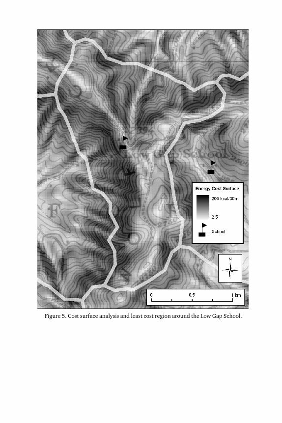
Figure 5. Cost surface analysis and least cost region around the Low Gap School.


province that dominates the study area,he is confident that ‘‘the geometric pat-terns of settlement, much more difficult tochange [than other aspects of materialculture], became prototypes for the rest ofthe Mountain South’’ (1978, p 206). Hismeticulous diagrams indicate that neigh-borhoods contained between 11 and 49farms, closely corresponding to ethno-graphic reports (Wilhelm 1978). For ex-ample, Brown’s Beech Creek census of 164people in 31 houses and Martin’s Holly-bush Hollow count of 150 people living on30 farms agree and are representative(Martin 1984; Brown 1988).

The agricultural neighborhoods de-rived from the HGIS analysis performedhere return representative buildingcounts. The 55 agricultural neighbor-hoods averaged 17 structures and 43neighborhoods (78 percent) were withinWilhelm’s range of 11 to 49 homes. Theremaining twelve zones were smaller, con-taining 10 or fewer buildings. A two-structure zone that contained a singlestructure and a schoolhouse was reallo-cated to adjacent zones, leaving 54 agri-cultural neighborhoods. The other 11small zones contained 4 and 9 farmhousesaround a country school, enough for sev-eral dozen relatives to form a kinshipneighborhood. Figure 6 displays the final54 agricultural neighborhoods and 24hamlets within the study area. The emptybuffer inside the study area and partiallysurrounding these 78 shaded regions wasoriginally occupied by the 32 least costzones that crossed the study area bounda-ries. Figure 6 also serves a reference mapshowing the places named in the abovediscussion.

The secondary literature suggests thatthere should be little difference between

agricultural neighborhoods and hamletsin absolute terms of structures and geo-graphic size. Hamlets and their surround-ing communities in the study area aver-aged 20 structures. Large hamlets, likeGreen Sulphur Springs, had around 50structures within their vicinities and thesmallest, like True, had a half dozen.

Multiplication of Wilhelm’s range of 11to 49 farmhouses per neighborhood by theaverage 1910 Appalachian farm size of 42hectares, suggests that agricultural neigh-borhoods should have ranged in size from462 to 2,058 hectares. By 1940, farmsaveraged 33 hectares, lowering the rangeto between 363 and 1,617 hectares. Gen-erally consistent with these calcula-tions, the 54 zones centered on schoolsand churches averaged 606 hectares of po-tential neighborhood area with a medianof 579 hectares and ranged from 250 to1,445 hectares.

Unlike size measures, density ratios di-rectly address the contrast between dis-persed neighborhoods of farmsteads andclustered hamlets. Historical researchersconcur that regardless of geomorphologi-cal setting, farms were dispersed withinneighborhoods. In linear hollows, farmhouses spread about 800 meters apartalong streams (Wilhelm 1978; Brown1988). In fan-shaped hollows, farmsteadsat headwaters and stream confluenceswere 150 meters from one another. Incoves, several dwellings clustered at thestream outlet and the rest were dispersedaround the basin’s periphery. Ridge settle-ment was linear with about 150 metersseparating farmers’ residences (Wilhelm1978). These observations establish arange of 150 and 800 meters betweenfarms.

Calculating dispersion based on small

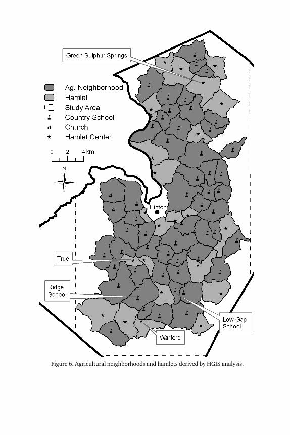
Figure 6. Agricultural neighborhoods and hamlets derived by HGIS analysis.


and large Summers County farm sizesleads to nearly identical figures. From1880 to 1930, about 90 percent of Sum-mers County farms occupied between 8and 202 hectares. Farmsteads centeredwithin evenly dispersed very small eighthectare farms will be 160 meters apart;those on 202 hectare farms will be 802meters apart.

HGIS analysis converted these dis-tances into four density categories. Twoare non-agricultural—‘‘commercial’’ and‘‘vacant’’—and two correspond to farming—‘‘general agricultural density’’ and ‘‘ar-chetypal agricultural density.’’ Maximumdensity expectations for agriculture derivefrom a hypothetical area divided into verysmall farms of eight hectares. A 40 hectaresearch area centered on each raster cellaccommodates 5 very small farms. There-fore, 6 or more structures within thesearch area suggest that land use is ‘‘com-mercial’’ and typical of a hamlet. The mini-mum agricultural density is that of anarea exclusively occupied by very large202 hectare farms with their farmsteadsspaced 800 meters apart. Land furtherthan 800 meters from a structure is notlikely to be farmland and is classified as‘‘vacant.’’ Only 2 percent of the study area,however, was this remote and two-thirdsof the least cost zones did not contain any‘‘vacant’’ land.

I characterize land at ‘‘general agri-cultural’’ density levels as follows: the min-imum density is a single house within800 meters; the maximum density is fivehouses within the surrounding 40 hect-ares. A narrower density sub-category, ‘‘ar-chetypal agricultural,’’ corresponds to alandscape of evenly spaced 40 hectarefarms, the average farm size in the countyfrom 1900 to 1930. Allowing for slightly

uneven spacing expands expectations by afarmstead on either side, or an ‘‘archetypalagricultural’’ density range from zero totwo farms within the search area.

Two expectations follow from the estab-lishment of these density categories. First,an overwhelming majority of the landwithin zones assumed to be agriculturalneighborhoods should be at ‘‘archetypalagricultural’’ densities. Second, even thosezones assumed to be hamlets should beprimarily farmland but should also containa relatively greater minority share of ‘‘com-mercial’’ density. Remember that as in thecases of Green Sulphur Springs, True, andWarford described above, farms fringedhamlets’ tiny commercial cores, leading tothe expectation that agricultural densitiespredominated within hamlet zones.

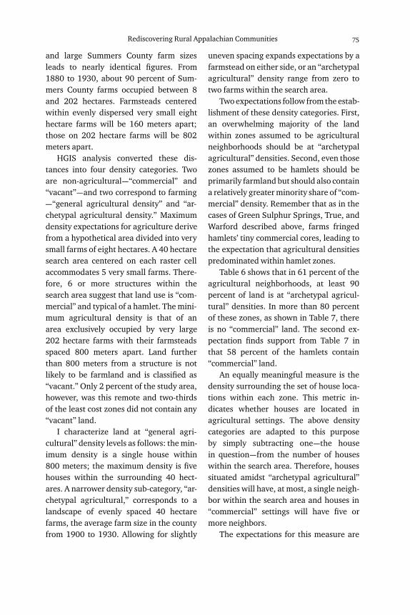
Table 6 shows that in 61 percent of theagricultural neighborhoods, at least 90percent of land is at ‘‘archetypal agricul-tural’’ densities. In more than 80 percentof these zones, as shown in Table 7, thereis no ‘‘commercial’’ land. The second ex-pectation finds support from Table 7 inthat 58 percent of the hamlets contain‘‘commercial’’ land.

An equally meaningful measure is thedensity surrounding the set of house loca-tions within each zone. This metric in-dicates whether houses are located inagricultural settings. The above densitycategories are adapted to this purposeby simply subtracting one—the housein question—from the number of houseswithin the search area. Therefore, housessituated amidst ‘‘archetypal agricultural’’densities will have, at most, a single neigh-bor within the search area and houses in‘‘commercial’’ settings will have five ormore neighbors.

The expectations for this measure are

76 george towers

Table 6. Archetypal agricultural density.

Percent of archetypal agricultural land

39–49% 50–79% 80–89% 90–95% 96–100% Total

Agricultural neighborhoods, N, (%) 0

(0%)

7

(13%)

14

(26%)

20

(37%)

13

(24%)

54

(100%)

Hamlets, N, (%) 2

(8%)

6

(25%)

8

(33%)

7

(29%)

1

(4%)

24

(100%)

Table 7. Commercial density.

Percent of commercial land

0% 1–5% 6–15% 16–44% Total

Agricultural neighborhoods, N, (%) 44

(81%)

10

(19%)

0

(0%)

0

(0%)

54

(100%)

Hamlets, N, (%) 10

(42%)

6

(25%)

7

(29%)

1

(4%)

24

(100%)

straightforward: more houses in hamletsshould be in ‘‘commercial’’ settings andmore houses in agricultural neighbor-hoods should be in areas of ‘‘archetypalagricultural’’ density. These expectationsare borne out by a variety of calculations.In agricultural neighborhoods, 2 of every3 houses (596 of 903) are in ‘‘archetypalagricultural’’ settings and only 1 in 50 (15of 903) are in ‘‘commercial’’ areas. Forty-nine of 54 agricultural neighborhoods (91percent) do not contain any houses in‘‘commercial’’ areas. In and around ham-lets, houses in ‘‘archetypal agricultural’’settings fall to 41 percent of the total whilethose in ‘‘commercial’’ areas increase to 28percent. Of the 793 houses in ‘‘archetypalagricultural’’ settings, three-fourths are inagricultural neighborhoods; of the 151houses in ‘‘commercial’’ areas, nine-tenthsare in hamlets.

This consistency within zones in termsof size and density is a function of theeven spacing of community nodes and theuniformity of farmhouse density. The reg-ularly dispersed pattern of communitynodes has less than a one percent like-lihood of occurring randomly accordingto nearest neighbor analysis. Farmhousedensity is also constant: 89 percent of theland in the 78 zones is at ‘‘archetypal agri-cultural’’ densities. Because both catego-ries of point features are evenly spacedacross the landscape, zones are certain tocontain homogenous settlement patterns.The equivalencies between farmhousedensity and zone sizes with those sug-gested by census data and ethnographicobservations assure these patterns’ fidelityto expectations from secondary sources. Inother words, the above analysis merelytranslates the organizational logic of agri-


cultural neighborhood settlement patternsinto numerical terms.

conclusions

This research presents an HGIS meth-odology that reliably locates the Appala-chian agricultural neighborhoods of a cen-tury ago. The least cost zones generatedby HGIS analysis of cultural features re-corded on early topographic maps sharethe spatial signature of the early 20th cen-tury southern Appalachian agriculturalneighborhoods described by ethnogra-phers and cultural geographers.

The methodology presented here is alsosignificant for its replicability. The primarydata sources, geo-referenced historic to-pographic maps and modern topographiccoverages, are freely downloadable forHGIS analysis. The principal analyticalmethod, cost allocation analysis, is a stan-dard, transparent GIS tool that requiresonly modest GIS proficiency.

Supported by the regional representa-tiveness of the study area, the method maybe applied by scholars across the socialand environmental sciences to reconstructhistoric southern Appalachian rural socialspace and extend our understanding ofthe region’s historical geography and con-temporary cultural landscape. For exam-ple, in archeology the inventorying of his-toric maps to analyze past settlementpatterns is a fundamental HGIS applica-tion (Harris 2002; Armstrong et al. 2008).As students of the southern Appalachiancountryside attest, once ubiquitous majorlandscape artifacts like the log cabins andcompany houses represented on old topo-graphic maps are rapidly vanishing (Re-hder 2004; DellaMea 2009). Archeolo-

gists may find this topographic HGISmethod useful as they search for and inte-grate the remaining traces of material cul-ture representing 19th century southernAppalachian society.

Historical geographers might use thisresearch method to explore Francaviglia’sobservation that ‘‘one of the greatest vi-sual contrasts in our culture occurs as onecrosses the line from agriculture to min-ing’’ (1991, p 5). This passage resonateswith Figure 7, which shows structures ona panel of contemporaneous USGS topo-graphic maps. The coal camps aroundWinona and those strung between Gentryand Backus comprised the eastern flank ofFayette County’s New River coalfield andstand out from the surrounding farm-lands. For southern Appalachia, the juxta-position of these two landscapes is a dual-ism that defines the region’s history. Themethodologies presented here invite in-quiry not only into how the coalfield-countryside boundary shifted over timeand space, but also may inform questionsabout the complementarity of these settle-ment patterns.

For historical sociologists and socialgeographers, topographic HGIS analysismight address the social and economic dif-ferences long observed between valley andridge communities. Early on, environmen-tal advantages found socioeconomic ex-pression. Valleys offering access to waterand good farmland were settled first andsupported the region’s leading rural com-munities (Wilhelm 1978). Ridge commu-nities, physiographically denied theseamenities, were afflicted by the notorioussouthern Appalachian ‘‘culture of poverty’’(Weller 1965; Gallaher 1974). Determin-ing whether the topography of socioeco-

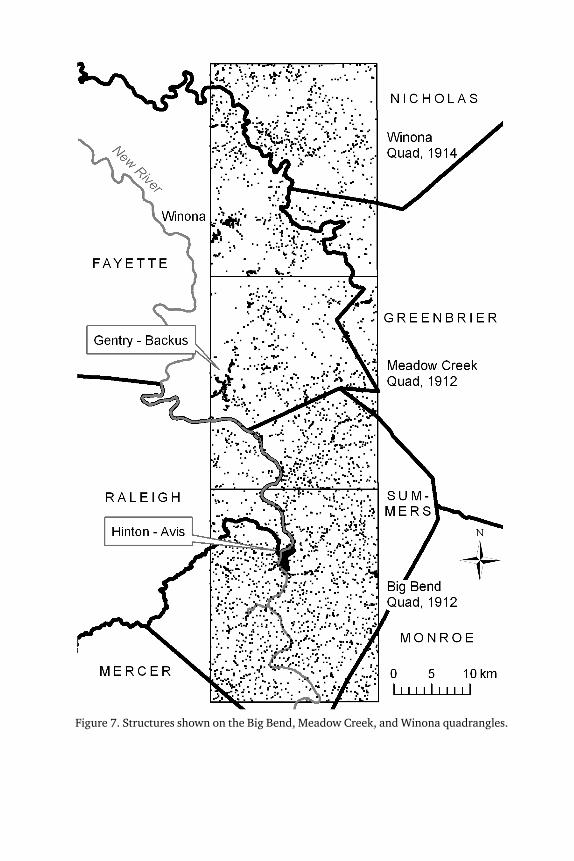
Figure 7. Structures shown on the Big Bend, Meadow Creek, and Winona quadrangles.


nomic status persists or has been reversedwith rural sprawl as suggested in recentCanadian research (Paquette and Domon2001) will contribute to our understand-ing of contemporary Appalachia.

Finally, for geographers, planners, andlandscape ecologists studying ‘‘ruralsprawl,’’ the low density settlement patternthat encircles many small towns and flanksrural roadways (Daniels 1999), topo-graphic HGIS provides important context.Like metropolitan sprawl, rural sprawl islamented for its encroachment on farm-land and wilderness, its infrastructural de-mands, and its centrifugal effects on com-munity (Daniels 1999; Reeder et al. 2001).While GIS-based assessment of sprawl’scosts is a burgeoning research area, it istypically made on the basis of relativelyrecent changes (Hasse and Lathrop 2003;Burchell et al. 2005; Wolman et al. 2005).Topographic HGIS puts recent landscapechange in historical perspective, allowingfor a richer assessment of rural sprawl’senvironmental impact.

The digitally driven ‘‘democratizationof cartography’’ empowers diverse scholar-ship with GIS (Slocum et al. 2009). Be-yond the reconstruction of southern Ap-palachian agricultural neighborhoods, thegoal of this study is to invite others toput topographic HGIS to their researchpurposes.

acknowledegment

The author thanks the editors and anony-

mous reviewers for their very helpful suggestions.

references

Ambler, C.H. 1951. A History of Education in

West Virginia: From Early Colonial Times to

1949. Huntington, WV: Standard Printing

and Publishing Company.

Armentrout, W.W. 1941. The Low-Income Farm

Situation in West Virginia As We Know It. In

Bulletin 299: Proceedings of the 1940

Conference on Low-Income Farms, 12–16.

Morgantown: Agricultural Experiment

Station, West Virginia University.

Armstrong, D.V., M.W. Hauser, D.W. Knight,

and S. Lenik. 2008. Maps, Matricals, and

Material Remains: An Archeological GIS of

Late-Eighteenth-Century Historic Sites on

St. John, Danish West Indies. In Archaeology

and Geoinformatics: Case Studies from

the Caribbean, ed. B.A. Reid, 99–126.

Tuscaloosa: University of Alabama Press.

Baker, A.R.H. 2003. Geography and History:

Bridging the Divide. Cambridge: Cambridge

University.

Beaver, P.D. 1976. Symbols and Social

Organization in an Appalachian Mountain

Community. Ph.D. Dissertation, Department

of Anthropology, Duke University.

Bell, T., and G. Lock. 2000. Topographic and

Cultural Influences on Walking the

Ridgeway in Later Prehistoric Times. In

Beyond the Map: Archaeology and Spatial

Technologies, ed. G. Lock, 85–100.

Amsterdam: IOS Press.

Billings, D.B., and Blee, K.M. 2000. The Road to

Poverty: The Making of Wealth and Hardship

in Appalachia. Cambridge: Cambridge

University Press.

Brown, J.S. 1988. Beech Creek: A Study of a

Kentucky Mountain Neighborhood. Berea,

KY: Berea College Press.

Burchell, R.W., Downs, A., McCann, B., and

Mukherji, S. 2005. Sprawl Costs: Economic

Impacts of Unchecked Development.

Washington: Island Press.

Colten, C.E., P.J. Hugill, T. Young, and K.M.

Morin. 2005. Historical Geography. In

Geography in America at the Dawn of the 21st

Century, eds. G.L. Gaille and C.J. Willmott,

149–163. Oxford: Oxford University.

80 george towers

Conolly, J., and LakeM. 2006. Geographical

Information Systems in Archaeology.

Cambridge: Cambridge University.

Cottle, R.K. 1997. Cemetery Siting in the

Bluestone Reservation Area, Summers

County, West Virginia: 1750–1997. M.S. Thesis,

Department of Geography, Virginia

Polytechnic Institute and State University.

Cunfer, G. 2005. On the Great Plains:

Agriculture and Environment. College

Station: Texas A&M University Press.

Daniels, T. 1999. What to Do About Rural

Sprawl? Paper presented at the American

Planning Association Conference, Seattle.

Dawson, A., Donaldson, K., Elmes, A., and

Gormont, J. 2007. WV Historical Geospatial

Products. Morgantown: West Virginia GIS

Technical Center.

DellaMea, C. 2009. Southern West Virginia

Coalfields. Accessed 31 July 2009 at http://

www.coalcampusa.com/sowv/index.html.

DeYoung, A.J., and Lawrence, B.K. 1995. On

Hoosiers, Yankees, and Mountaineers. Phi

Delta Kappan 77(2):104–112.

Dunn, D. 1988. Cades Cove: The Life and Death

of a Southern Appalachian Community,

1818–1937. Knoxville: University of

Tennessee Press.

Dunne, F. 1977. Choosing Smallness: An

Examination of the Small School

Experience in Rural America. In Education

in Rural America, ed. J.P, Sher, 81–124.

Boulder, CO: Westview Press.

Eller, R.D. 1982. Miners, Millhands, and

Mountaineers: Industrialization of the

Appalachian South, 1880–1930. Knoxville:

University of Tennessee Press.

———. 2008. Uneven Ground: Appalachia since

1945. Lexington: University Press of

Kentucky.

Ferguson, L.M. 1950. The Educational

Development of Mercer County. M.A. Thesis,

Department of Education, Marshall College.

Francaviglia, R.V. 1991. Hard Places: Reading

the Landscape of America’s Historic Mining

Districts. Iowa City: University of Iowa

Press.

Gallaher, A., Jr. 1974. The Community as a

Setting for Change in Southern Appalachia.

In Appalachia: Its People, Heritage, and

Problems, ed. F.S. Riddel, 291–304.

Dubuque, IA: Kendall/Hunt Publishing

Company.

Gragson, T.L., and Bolstad, P.V. 2007. A Local

Analysis of Early-Eighteenth-Century

Cherokee Settlement. Social Science History

31(3):435–468.

Gregory, I.N., and Healey, R.G. 2007. Historical

GIS: Structuring, Mapping and Analysing

Geographies of the Past. Progress in Human

Geography 31(5):638–653.

Gulliford, A. 1996. America’s Country Schools,

3rd Edition. Niwot, CO: University Press of

Colorado.

Harris, T.M. 2002. GIS in Archaeology. In Past

Time, Past Place: GIS for History, ed. A.K.

Knowles, 131–142. Redlands, CA: ESRI

Press.

Hart, J.F. 1975. The Look of the Land.

Englewood Cliffs, NJ: Prentice-Hall, Inc.

Hasse, J., and Lathrop, R.G. 2003. A Housing-

Unit-Level Approach to Characterizing

Residential Sprawl. Photogrammetric

Engineering & Remote Sensing 69(9):1021–

1030.

Helbock, R.W. 2004. United States Post Offices,

Volume VI—The Mid-Atlantic. Scappoose,

OR: La Posta Publications.

Holy, T.C. 1929. Survey of Education in West

Virginia, Volume III: School Buildings.

Charleston: West Virginia State Department

of Education.

Howell, B.J. 2003. Folklife along the Big South

Fork of the Cumberland River. Knoxville:

University of Tennessee Press.

Hunter, R.W. 2009. People, Sheep, and Landscape


Change in Colonial Mexico: The Sixteenth-

Century Transformation of the Valle Del

Mezquital. Ph.D. Dissertation, Department

of Geography and Anthropology, Louisiana

State University.

Kaplan, B.H. 1971. Blue Ridge: An Appalachian

Community in Transition. West Virginia

University Bulletin 71:(7/2).

King, M.L., and Magnuson, D.L. 1995.

Perspectives on Historical U.S. Census

Undercounts. Social Science History

19(4):455–466.

Knowles, A.K. 2008. GIS and History. In Placing

History: How Maps, Spatial Data, and GIS

Are Changing Historical Scholarship, eds.

A.K. Knowles and A. Hillier, 1–26.

Redlands, CA: ESRI Press.

Mann, R. 1995. Diversity in the Antebellum

Appalachian South: Four Farm Communities

in Tazewell County, Virginia. In Appalachia

in the Making: The Mountain South in the

Nineteenth Century, eds. M.B. Pudup, D.B.

Billings, and A.L. Waller, 132–162. Chapel

Hill: University of North Carolina Press.

Martin, C.E. 1984. Hollybush: Folk Building

and Social Change in an Appalachian

Community. Knoxville: University of

Tennessee Press.

Matthews, E.M. 1965. Neighbor and Kin: Life in

a Tennessee Ridge Community. Nashville:

Vanderbilt University Press.

Miller, J.H. 1908. History of Summers County,

West Virginia from the Earliest Settlement to

the Present Time. Hinton, WV: James H.

Miller.

Minetti, A.E., Moia, C., Roi, G.S., Susta, D., and

Ferretti, G. 2002. Energy Cost of Walking

and Running at Extreme Uphill and

Downhill Slopes. Journal of Applied

Physiology 93:1039–1046.

Newcomb, J.C. 2008. Interview with W.J.

Daniels and author. Lynco, WV,

December 30.

Paquette, S., and Domon, G. 2001. Trends in

Rural Landscape Development and

Sociodemographic Recomposition in

Southern Quebec (Canada). Landscape and

Urban Planning 55:215–238.

Parkerson, D.H. 1991. Comments on the

Underenumeration of the U.S. Census,

1850-1880. Social Science History

15(4):509–515.

Pearsall, M. 1959. Little Smoky Ridge: The

Natural History of a Southern Appalachian

Neighborhood. Birmingham: University of

Alabama Press.

Photiadis, J.D. 1980. The Changing Rural

Appalachian Community and Low-Income

Family: Implications for Community

Development. West Virginia University

Bulletin 80(9/7).

Reeder, R., Brown, D., and McReynolds, K.

2001. Rural Sprawl: Problems and Policies

in Eight Rural Counties. The Small City and

Regional Community: Proceedings of the

2000 Conference 14:199–206.

Rehder, J.B. 2004. Appalachian Folkways.

Baltimore: Johns Hopkins University Press.

Reynolds, D.R. 1999. There Goes the

Neighborhood: Rural School Consolidation at

the Grass Roots in Early Twentieth-Century

Iowa. Iowa City: University of Iowa Press.

Robinson, J.G. 1988. Perspectives on the

Completeness of Coverage of Population in

the United States Decennial Censuses.

Paper presented at the Annual Meeting of

the Population Association of America.

Salstrom, P. 1994. Appalachia’s Path to

Dependency: Rethinking a Region’s Economic

History, 1730–1940. Lexington: University

Press of Kentucky.

Sanders, W. 1992. A New River Heritage,

Volume II. Parsons, WV: McClain Printing

Company.

Slocum, T.A., R.B. McMaster, F.C. Kessler, and

H.H. Howard. 2009. Thematic Cartography

82 george towers

and Visualization, 3rd Edition. Upper Saddle

River, NJ: Pearson/Prentice Hall.

Stephenson, J.B. 1968. Shiloh: A Mountain

Community. Lexington: University of

Kentucky Press.

Summers County Historical Society. 1984. The

History of Summers County, West Virginia.

Marceline, MO: Walsworth Press.

Thomas, J.B. 1998. An Appalachian New Deal:

West Virginia in the Great Depression.

Lexington: University Press of Kentucky.

Trent, W.W. 1960. Mountaineer Education: A

Story of Education in West Virginia 1885–

1957. Charleston, WV: Jarrett Printing

Company.

United States Census. 1910. Thirteenth Census

of the United States, 1910—Population,

Microfilm Roll 1694 Pocahontas, Putnam

and Summers Counties, West Virginia.

Washington: U.S. Census.

United States Census. 1913. Thirteenth Census

of the United States: 1910—Volume 7:

Agriculture: Reports by States, Nebraska—

Wyoming, Alaska, Hawaii, Puerto Rico.

Washington: U.S. Census.

University of Virginia, Geospatial and

Statistical Data Center. 2004. Historical

Census Browser. http://fisher.lib.virginia

.edu/collections/stats/histcensus/index

.html.

Unrau, H.D. 1996. New River Gorge National

River, West Virginia: Special History

Study/Historic Context Study. Washington:

National Park Service, U.S. Department of

the Interior.

Weller, J.E. 1965. Yesterday’s People: Life in

Contemporary Appalachia. Lexington:

University of Kentucky Press.

Wheatley, D., and Gillings, M. 2002. Spatial

Technology and Archaeology: The

Archaeological Applications of GIS. New

York: CRC Press.

Wilhelm, G., Jr. 1978. Folk Settlements in the

Blue Ridge Mountains. Appalachian Journal

5(2):204–245.

Williams, J.A. 2001. Appalachia: A History.

Chapel Hill: University of North Carolina

Press.

Winkle, K. 1991. The U.S. Census as a Source in

Political History. Social Science History

15(4):565–577.

Wolman, H., Galster, G., Hanson, R.,

Ratcliffe, M., Furdell, K., and Sarzynski, A.

2005. The Fundamental Challenge in

Measuring Sprawl: Which Land Should Be

Considered? Professional Geographer

57(1):94–105.

george towers is a Professor of Geography

and Associate Academic Dean at Concord

University, Athens, WV 24712. Email:

[email protected]. His research interests

involve the human geography of Appalachia.

rediscovering rural appalachian communities with historical gis

Documents