reconfiguration and communication-aware task scheduling for high-performance reconfigurable...

Reconfiguration and Communication-Aware TaskScheduling for High-Performance ReconfigurableComputing

MIAOQING HUANG, VIKRAM K. NARAYANA, HARALD SIMMLER,

OLIVIER SERRES and TAREK EL-GHAZAWI

NSF Center for High-Performance Reconfigurable Computing (CHREC)

The George Washington University

High-performance reconfigurable computing involves acceleration of significant portions of an ap-

plication using reconfigurable hardware. When the hardware tasks of an application cannot si-multaneously fit in an FPGA, the task graphs needs to be partitioned and scheduled into multiple

FPGA configurations, in a way that minimizes the total execution time. This paper proposes

the Reduced Data Movement Scheduling (RDMS) algorithm that aims to improve the overallperformance of hardware tasks by taking into account the reconfiguration time, data dependency

between tasks, inter-task communication as well as task resource utilization. The proposed algo-

rithm uses the dynamic programming method. A mathematical analysis of the algorithm showsthat the execution time would at most exceed the optimal solution by a factor of around 1.6, in

the worst-case. Simulations on randomly generated task graphs indicate that RDMS algorithm

can reduce inter-configuration communication time by 11% and 44% respectively, compared withtwo other approaches that consider data dependency and hardware resource utilization only. The

practicality, as well as efficiency of the proposed algorithm over other approaches, is demonstrated

by simulating a task graph from a real-life application - N-body simulation - along with constraintsfor bandwidth and FPGA parameters from existing high-performance reconfigurable computers.

Experiments on SRC-6 are carried out to validate the approach.

Categories and Subject Descriptors: B.8.2 [PERFORMANCE AND RELIABILITY]: Per-formance Analysis and Design Aids; C.1.3 [PROCESSOR ARCHITECTURES]: Other Ar-

chitecture Styles—Adaptable architectures

General Terms: Algorithms, Design

Additional Key Words and Phrases: Hardware Task Scheduling, Reconfigurable Computing

1. INTRODUCTION

High-performance reconfigurable computers (HPRCs) are traditional HPCs ex-tended with co-processors based on reconfigurable hardware like FPGAs. Theseenhanced systems are capable of providing significant performance improvement

Authors’ address: M. Huang, V.K. Narayana, H. Simmler, O. Serres and T. El-Ghazawi, Depart-ment of Electrical and Computer Engineering, The George Washington University, Ashburn, VA

20147, USA; email: [email protected], [email protected], [email protected],[email protected], [email protected] to make digital/hard copy of all or part of this material without fee for personalor classroom use provided that the copies are not made or distributed for profit or commercial

advantage, the ACM copyright/server notice, the title of the publication, and its date appear, andnotice is given that copying is by permission of the ACM, Inc. To copy otherwise, to republish,

to post on servers, or to redistribute to lists requires prior specific permission and/or a fee.c© 200Y ACM xxxx-xxxx/200Y/xxxx-0001 $5.00

ACM Transactions on Reconfigurable Technology and Systems, Vol. V, No. N, MM 200Y, Pages 1–24.

2 · M. Huang et al.

User Logic(IP)

Vendor-Specific Service Logic

FPGA DeviceLocal Memory

Bank 0

Local Memory Bank 1

Local Memory Bank n-1

Micro-processor

HostMemory Interconnect

DMA

Fig. 1. The General Architecture of A High-Performance Reconfigurable Computer

for scientific and engineering applications. Well known HPRC systems such asCray XD1, the SRC-6, and SGI RC100 use a high-speed interconnect, shown inFigure 1, to connect the general-purpose µP to the co-processor.

Early attempts to improve the efficiency of FPGA co-processors used task place-ment algorithms in combination with partial run-time reconfiguration or dynamicreconfiguration to reduce the configuration overhead of the FPGA system [Feketeet al. 2001; Bazargan et al. 2000; Diessel et al. 2000; Walder and Platzner 2002;Brebner and Diessel 2001; Compton et al. 2002; Walder et al. 2003; Handa and Ve-muri 2004]. Most of these map individual SW functions onto the FPGA to acceler-ate the whole application; however, the optimization strategies for task placementdid not consider data communication or data dependencies among hardware tasks.

We believe that an optimized hardware task scheduling algorithm has to take taskdependencies, data communication, task resource utilization and system parame-ters into account to fully exploit the performance of an HPRC system. This paperpresents an automated hardware task scheduling algorithm that is able to map sim-ple and advanced directed acyclic graphs (DAG) in an optimized way onto HPRCsystems. More precisely, it is able to split a DAG onto multiple FPGA configura-tions optimizing the overall execution of the hardware part of the user application,after the HW/SW partition has been done. The optimization is achieved by mini-mizing the number of FPGA configurations and minimizing the inter-configurationcommunication overhead between the FPGA device and external memory by usinga data dependency analysis of the given DAG. Maximum concurrency in hardwareprocessing is ensured by considering pipeline chaining of hardware tasks within thesame FPGA configuration.

The remaining text is organized as follows. Section 2 introduces the relatedwork. Section 3 presents the hardware task scheduling algorithm, followed by amathematical analysis of the algorithm. Section 4 focuses on the results obtainedfor various graphs by using the proposed algorithm. The limitations of the proposedapproach are also outlined. Finally, Section 5 concludes this paper.

2. RELATED WORK

Early work on hardware task placement for reconfigurable hardware focused onreducing configuration overhead and therefore improving the efficiency of reconfig-urable devices. In [Fekete et al. 2001], an offline 3D module placement approachfor partially reconfigurable devices was presented. Efficient data structures and al-gorithms for fast online task placements and simulation experiments for variants offirst fit, best fit and bottom left bin-packing algorithms are presented in [BazarganACM Transactions on Reconfigurable Technology and Systems, Vol. V, No. N, MM 200Y.

Reconfiguration and Communication-Aware Task Scheduling for HPRCs · 3

…... FPGAConfiguration

HW Data Processing

FPGAConfiguration

DataCommunication …...Data

Communication

time

process cycle

Fig. 2. The Basic Execution Model of Hardware Tasks on FPGA Device

et al. 2000]. In [Diessel et al. 2000], the fragmentation problem on partially re-configurable FPGA devices was addressed. Task rearrangements were performedby techniques denoted as local repacking and ordered compaction. In [Walder andPlatzner 2002], non-rectangular tasks were explored such that a given fragmenta-tion metric was minimized. Furthermore, a task’s shape may be changed in orderto facilitate task placement. In [Brebner and Diessel 2001], a column-oriented one-dimensional task placement problem was discussed. Task relocations and trans-formations to reduce fragmentation were proposed in [Compton et al. 2002] basedon a proposed FPGA architecture that supported efficient row-wise relocation. In[Walder et al. 2003], three improved partitioning algorithms based on [Bazarganet al. 2000] were presented. In [Handa and Vemuri 2004], a fast algorithm forfinding empty rectangles in partially reconfigurable FPGA device was presented.However, these algorithms only focused on utilizing the FPGA device efficientlythrough optimal task placement techniques and did not address the performanceoptimization among tasks in a given application, which is the main concern of theusers of an HPRC system.

More recently, HW/SW co-design algorithms for RC systems have emerged,bringing the ease of use urgently needed in the RC domain. In [Wiangtong et al.2003], a HW/SW co-design model comprised of a single µP and an array of hard-ware processing elements (PEs implemented on FPGAs) was presented. Small tasksin a user program were dynamically assigned onto PEs. However, even if a singlePE could accommodate multiple tasks, the tasks were executed in a sequentialway. In [Saha 2007], an automatic HW/SW co-design approach on RCs was pro-posed. The proposed ReCoS algorithm partitioned a program into hardware tasksand software tasks and co-scheduled the tasks on their respective PEs. Althoughthe ReCoS algorithm places multiple hardware tasks into the same configuration,each task is treated as a stand-alone hardware module. No data paths are definedbetween the tasks even if they reside in the same configuration.

3. REDUCED DATA MOVEMENT SCHEDULING ALGORITHM

Given the hardware task graph of one application and the hardware implementationof each task, the RDMS algorithm schedules the hardware tasks into a series ofFPGA configurations in a way that minimizes the total hardware execution time,by restricting the number of FPGA configurations and the transfer of intermediatedata between FPGA and host memory [Huang et al. 2009]. In order to achieve thesedesired objectives, the RDMS algorithm takes three factors into account duringthe scheduling process, namely, (a) the task data dependencies, (b) the hardwareresource utilization of each task, and (c) the inter-task data communication.

RDMS assumes the execution model shown in Figure 2, for hardware tasks run-ning on the FPGA co-processor. After the FPGA device is configured and before

ACM Transactions on Reconfigurable Technology and Systems, Vol. V, No. N, MM 200Y.


hardware tasks start their computation, raw data are transferred from the µP or ex-ternal memory to the FPGA device. After hardware tasks finish their computation,the processed data are transferred back from the FPGA device to external mem-ory, before the next FPGA configuration is loaded into the device∗. The data fromexternal memory are then again transferred to the FPGA, in order to feed tasksthat have a dependency on other tasks that finished computation in the precedingconfiguration(s).

In addition to the assumption of the execution model shown in Figure 2, theRDMS algorithm uses the following assumptions about the underlying system:

(1) Implementation of all tasks are pipelined, allowing concurrent execution of taskswithin a configuration. (If the tasks are not inherently pipelined, FIFO buffersat the input and output of the tasks can be used, to create a similar effect.)

(2) The data processed by each FPGA configuration is large, allowing the initialpipeline latency to be neglected.

(3) FPGA supports only full configuration (partial reconfiguration is not allowed).

The processing time of each task is the ratio of input data volume for the taskand data consumption throughput of the task. From assumptions 1 and 2, it fol-lows that the processing time of a particular FPGA configuration simply equalsthe processing time of the slowest task in the configuration. The time taken fordata transfer between the host memory and FPGA is computed based on the in-terconnect bandwidth and the data volume transfer to/from the task edges. Theexecution time Thwe for the entire computation consisting of n configurations is,therefore, the sum of (1) n · TR, in which TR is the configuration time of the wholeFPGA device, (2) the processing time of slowest task in each configuration, and (3)host memory data transfer time for each configuration.

As mentioned earlier, configuration time and data communication time are pureoverheads for using RCs and therefore both should be reduced to a minimum. Twostrategies are applied to achieve this objective.

(1) Execute as many tasks as possible in one FPGA configuration to minimize theamount of configurations. This will reduce the configuration overhead as wellas the communication overhead between tasks.

(2) Group communicating tasks into the same configuration to minimize thedata communication time and to maximize the performance achieved throughpipelining and concurrent task execution.

Given the DAG of an application, the overall amount of communication volumeamong the tasks is fixed. When the tasks of the DAG are scheduled into multipleFPGA configurations, the communication can be categorized into two types - theinternal communication inside FPGA configurations and the inter-configurationcommunication. Because the sum of these two categories of communication is fixed,we expect that minimization of the inter-configuration communication is equivalentto maximizing the internal communication inside FPGA configurations.

∗In most cases the data communication and data processing are overlapped due to the highthroughput of the hardware design. We intentionally distinguish these two times in this work for

the sake of simplicity.



H1 H2 H3 H4

H7H6H5

H10H9H8 H11

H12 H13

1 1 12

1 1

1

1

2 2 2

22

2

3

3

3

3

4

47

3

Node Sequence No.

Normalized Communication

Time

Node weight, i.e., normalized hardware resource utilization

Normalized node configuration time

H0: imaginary root node

(a) An Example DAG Consisting of 13Nodes

H1 H2 H3 H4

H7H6H5

H10H9H8 H11

H12 H13

(b) Scheduling Result of the ExampleDAG Using RDMS

Fig. 3. The Example Graph

We identified the required task scheduling as a dependent knapsack problem,which is a constrained case of the knapsack problem [Kellerer et al. 2004]. For thesingle-objective independent knapsack problem, there exists an exact solution thatcan be computed using a dynamic programming approach [Kleinberg and Tardos2005]. In the traditional knapsack problem, each object is associated with twoparameters, the weight and the profit. The weight can be seen as a penalty thathas to be paid for selecting an object and the profit is a reward. The goal of theknapsack problem is to maximize the profit subject to a maximum total weight.

In our task scheduling case, we have a dependent knapsack problem where wehave to take care of the task dependencies and make sure that all parent tasks havebeen scheduled before scheduling the corresponding child task. This ensures thatthe input data of every task is either obtained from host memory as a result of apreviously executed task, or through data forwarding from another task within thesame configuration.

The objects in the task scheduling knapsack problem are the hardware tasksgiven in the DAG. The weight of each object is the hardware resource utilization ofthe corresponding task. Because the objective of the knapsack problem is to max-imize the profit, we have to define the profit according to our two goals: maximizethe amount of tasks and minimize the inter-configuration communication betweentasks†. Both profits are transformed into a common unit, time, so that a singleunified metric for the profit can be used.

The number of tasks assigned to each configuration is dependent on the allocatedresources for each task. Therefore, we define one part of the profit to be the con-figuration time of each task. This “configuration time” is the fraction of the full

†Hardware processing time is not considered in the objective function for the algorithm, since the

communications and reconfigurable cost are greater than that time in most cases.



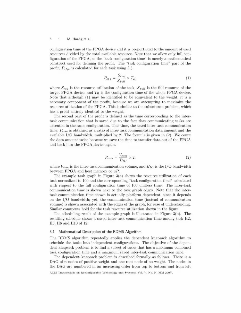
configuration time of the FPGA device and it is proportional to the amount of usedresources divided by the total available resource. Note that we allow only full con-figuration of the FPGA, so the “task configuration time” is merely a mathematicalconstruct used for defining the profit. The “task configuration time” part of theprofit, Pcfg, is calculated for each task using (1).

Pcfg =SreqSfull

× TR, (1)

where Sreq is the resource utilization of the task, Sfull is the full resource of thetarget FPGA device, and TR is the configuration time of the whole FPGA device.Note that although (1) may be identified to be equivalent to the weight, it is anecessary component of the profit, because we are attempting to maximize theresource utilization of the FPGA. This is similar to the subset-sum problem, whichhas a profit entirely identical to the weight.

The second part of the profit is defined as the time corresponding to the inter-task communication that is saved due to the fact that communicating tasks areexecuted in the same configuration. This time, the saved inter-task communicationtime, Pcom is obtained as a ratio of inter-task communication data amount and theavailable I/O bandwidth, multiplied by 2. The formula is given in (2). We countthe data amount twice because we save the time to transfer data out of the FPGAand back into the FPGA device again.

Pcom =VcomBIO

× 2, (2)

where Vcom is the inter-task communication volume, and BIO is the I/O bandwidthbetween FPGA and host memory or µP .

The example task graph in Figure 3(a) shows the resource utilization of eachtask normalized to 100 and the corresponding “task configuration time” calculatedwith respect to the full configuration time of 100 unitless time. The inter-taskcommunication time is shown next to the task graph edges. Note that the inter-task communication time shown is actually platform dependent, since it dependson the I/O bandwidth; yet, the communication time (instead of communicationvolume) is shown associated with the edges of the graph, for ease of understanding.Similar comments hold for the task resource utilization shown in the figure.

The scheduling result of the example graph is illustrated in Figure 3(b). Theresulting schedule shows a saved inter-task communication time among task H2,H3, H6 and H10 of 12.

3.1 Mathematical Description of the RDMS Algorithm

The RDMS algorithm repeatedly applies the dependent knapsack algorithm toschedule the tasks into independent configurations. The objective of the depen-dent knapsack problem is to find a subset of tasks that has a maximum combinedtask configuration time and a maximum saved inter-task communication time.

The dependent knapsack problem is described formally as follows. There is aDAG of n nodes of positive weight and one root node of no weight. The nodes inthe DAG are numbered in an increasing order from top to bottom and from leftACM Transactions on Reconfigurable Technology and Systems, Vol. V, No. N, MM 200Y.


to right at the same level. Each node is associated with a weight wi and a profitpi, 0 ≤ i ≤ n. The wi values correspond to the percentage of resource utilizationof each task, whereas the profit values pi associated with each task are computedusing (1). The profit derived from savings in inter-task communication is capturedby a matrix E‡; this matrix describes the links among the nodes and E(i, j) is theprofit associated with the edge between node i and j, computed using (2).

To solve the dependent knapsack problem, it is required to select a subset ofnodes S ⊆ {1, . . . , n} so that

∑i∈Swi ≤W (the given upper bound) and, subject

to two restrictions, namely,

—The profit of the selected subset S, given by∑i∈Spi + interc(S), is as large as

possible, where interc(S) is the profit due to the saved inter-task communication,as described in Equation (3):

interc(S) =∑

i,j∈S;i,j 6=0

E(i, j)§ (3)

—For all nodes i ∈ S, their parent nodes also belong to S, so that the concurrentexecution of all tasks and the internal data forwarding inside a single FPGAconfiguration becomes possible.

We use the dynamic programming approach to solve the dependent knapsackproblem. Dynamic programming relies on solving smaller subproblems in orderto eventually solve the original problem. Recursive relations are used in order toachieve the desired objective. Recursion is defined on the task subset S based onvariable index i and the weight (resource) constraint w; S(i, w) denotes the optimalsubset of tasks chosen from {1, . . . , i} under the weight constraint w. The objectiveof the dependent knapsack problem is to determine S(n,W ), where W is the fullFPGA resource constraint. Corresponding to S(i, w), we also have the maximalprofit values POPT (i, w). Since the choice of S(i, w) is essentially based on thetasks that result in maximal profit, we first define recursions on POPT (i, w). Usingthe notations wi and pi, the weight and profit of task i as defined in the beginningof Section 3.1, the recurrence relation for the maximal profit value POPT is:

POPT (i, w) =

(POPT (i− 1, w) if wi > w,

max(POPT (i− 1, w), [POPT (i− 1, w′) + pi + inter(i)]) Otherwise.

(4)

where inter(i) is a measure of the savings in inter-task communication based onthe inclusion of task i to the subset S(i−1, w′), to be quantified later. The variablew′ will also be formally defined later, but for this initial discussion let us considerit to be w′ = (w − wi). The principle behind Equation (4) is to obtain POPT (andtherefore S) for tasks {1, . . . , i}, based on the result for tasks {1, . . . , i − 1}.The basic idea is that if task i has a weight wi smaller than the weight constraint

‡The communication times between imaginary root node 0 and other nodes are not considered

during the calculation since the corresponding data are input data to the whole graph and have

to be transferred anyway. For the same reason, the final output of the DAG is not considered inthe calculation.§If there is no edge from i to j, E(i, j)=0.



Algorithm 1: Algorithm for Dependent Knapsack ProblemInput: Empty array POPT [0..n, 0..W ], S[0..n, 0..W ] and a DAG of

corresponding n nodes plus an imaginary root node 0. The nodes inthe DAG are numbered in an increasing order from top to bottom andfrom left to right at the same level. Each node is associated with oneweight wi and one profit pi. Matrix E[0..n, 0..n] describes the linkamong the nodes and the associated profit of each link in the DAG.

Output: POPT (n,W ) is the optimal profit combination and S(n,W ) containsthe corresponding nodes.

Initialize POPT [0, w] = S[0, w] = 0 for 0 ≤ w ≤W , and POPT [i, 0] = S[i, 0] = 01.1

for 0 ≤ i ≤ n;for i = 1 to n do1.2

for w = 1 to W do1.3

Use the recurrence Equations (4)-(5) to compute POPT (i, w) and fill in1.4

S(i, w);

w, then its inclusion in S implies that the other tasks chosen from {1, . . . , i − 1}comprise an optimal subset under the weight constraint w′ = (w − wi).

Corresponding to recurrence (4), the recurrence relation for task subset S maybe easily written down. From the first line of (4), if wi > w it follows thatS(i, w) = S(i− 1, w), which means that task i is not included in S(i, w). Thiscould also happen for line 2 of (4), when the profit POPT (i − 1, w) is the largerterm. The only case when task i is included in S(i, w) is when the overall profitdue to its inclusion will be larger than POPT (i− 1, w). These points are capturedsuccinctly as follows:

S(i, w) =

(S(i− 1, w) if wi > w or POP T (i− 1, w) > [POP T (i− 1, w′) + pi + inter(i)] ,

{S(i− 1, w′), i} Otherwise.(5)

The expression to compute inter(i), described earlier as the savings in inter-taskcommunication due to the inclusion of task i, is as follows:

inter(i) =∑

j∈S(i−1,w′),j 6=0

E(j, i) (6)

We have referred to w′ earlier as the weight constraint on the remaining taskschosen from {1, . . . , i − 1}, provided task i is included in S(i, w). Since task i isbeing considered for inclusion, the weight constraint on the remaining tasks wouldbe w−wi, which is accurate in the absence of precedence constraints among tasks.For our case, however, it might turn out that S(i− 1, w − wi) does not contain allof the parents of node i. In that case, starting from w−wi, the constraint w′ mustbe successively reduced until S(i − 1, w′) contains all the parents nodes of task i.That is,

w′ = max{x|x ≤ w − wi and all of node i ’s parent nodes belong to S(i− 1, x)} (7)

Note that the weight is a continuous variable, so it is discretized in steps of 1% ofmaximum FPGA resource constraint W , in order to determine w′ using (7). Basedon equations (4)-(7), the overall dynamic programming solution for the dependentACM Transactions on Reconfigurable Technology and Systems, Vol. V, No. N, MM 200Y.


Algorithm 2: RDMS AlgorithmInput: A DAG of n+ 1 nodes, representing n hardware tasks and an

imaginary root node 0. Each node i has a weight wi and a profit pi.Matrix E[0..n, 0..n] describes the link among the nodes and theassociated profit of each link in the DAG.

Output: A sequence of disjoint subsets {S1, . . . , Sj} satisfying∑i∈Sk

wi ≤W , k = 1, . . . , j.Let O denote the set of current remaining items and initialize O = {1, . . . , n},2.1

let k=1;while O is not empty do2.2

Apply Algorithm 1 on O and DAG to find the subset Sk;2.3

Remove the items in the subset Sk from O and corresponding nodes from2.4

the DAG;Connect those nodes whose parent nodes have been taken to the root node2.5

directly;k = k + 1;2.6

knapsack problem is given in Algorithm 1. As mentioned earlier, the output of thealgorithm is the required subset of tasks S(n,W ) with the corresponding maximalprofit POPT (n,W ). Algorithm 1 is used within the RDMS algorithm, which isdescribed next.

The RDMS algorithm begins with Algorithm 1 to schedule a subset of tasksinto the first configuration. Once this is done, the scheduled tasks (or nodes) areremoved from the DAG. Edges that connect the existing nodes to the deleted nodesare rearranged so that they are connected to the root node instead. Algorithm 1 isthen applied again to determine the second configuration. The process is repeateduntil all tasks in the DAG are scheduled. These steps are formally described inAlgorithm 2.

The example DAG shown in Figure 3(a) is scheduled using RDMS, and theresulting configurations are shown in Figure 3(b). The scheduled result consistsof four FPGA configurations, {H2,H3,H6,H10}, {H1,H9,H12,H4,H7}, {H5,H8} and{H11,H13}. In other words, the FPGA will be reconfigured four times. Eachconfiguration performs part of the computation on one piece of data.

By taking two system parameters, the configuration time of hardware tasks andthe inter-task communication time into account, the RDMS algorithm can addressthe characteristics of different platforms automatically. On an RC system with along configuration time, the configuration overhead of hardware tasks will play amore important role in the scheduling process. On a different RC system that canswitch from one configuration to the other instantly, but instead has a compara-tively slow interconnect, the algorithm will favor packing of tasks into the sameconfiguration if their inter-task data transfer is large.

3.2 Mathematical Analysis of the RDMS Algorithm

We carry out a formal analysis of the proposed RDMS algorithm, in order to deter-mine its time complexity, space requirements, as well as the worst-case performance



bounds.

3.2.1 Time Complexity. In order to compute each POPT (i, w) in the Algorithmfor Dependent Knapsack Problem, it traces back at most w − 1 steps, see Equa-tion (7). (The number of steps is based on the fact that the weight is expressed asa percentage of resource utilization, and because it is discretized in steps of 1% ofmaximum resource constraint, w is effectively an integer between 1 and 100) Fur-thermore, it may take n − 1 steps to check the solvability of each node under theworst-case scenario. Therefore, it takes O(nw) time to compute each POPT (i, w).The time to compute whole row is O(n+n× 2 + · · ·+n× (W − 1) +n×W ), whichis O(nW 2). The time complexity of the whole algorithm, i.e., n rows, is O(n2W 2).

In order to compute the time complexity of RDMS Algorithm, consider the worst-case scenario in which only one node is taken every iteration. Because the timecomplexity of Algorithm 1 is O(n2W 2) given n items and an upper bound W ,the time for calculating the sequence of subsets is O(n2W 2 + (n − 1)2W 2 + · · · +22W 2 +W 2), which is O(n3W 2). Since a breadth-first search technique is adoptedto reorganize the directed rooted graph (Line 2.5 of Algorithm 2), it takes O(n+E)time given n nodes and E edges among them. The maximum possible value of E isn2; hence, the time complexity of the reorganization is O(n+ n2), which is O(n2).The time complexity of the reorganization for the whole process is O(n2 + (n −1)2 + · · ·+ 22 + 1), which is O(n3). Altogether, the time complexity of Algorithm 2is O(n3W 2) under the worst-case scenario.

In [Pisinger 1999], Pisinger introduced an algorithm that is able to reduce thetime complexity of the independent knapsack problem by lowering W to w, wherew is the largest weight of an item in the instance. Further research is required tostudy the feasibility of similar optimizations for the RDMS algorithm.

3.2.2 Space Requirement. Since the RDMS algorithm runs the Algorithm forthe Dependent Knapsack Problem multiple times, the space requirement of theformer one is same as for the latter one.

For the Algorithm for the Dependent Knapsack Problem, the space requirementto save the information of n items will be O(n2) at the most. Because the compu-tation of both POPT (i, w) and S(i, w) relies only on the variables from the previousrow, only two rows of each of them are required during the processing. Therefore,the POPT array will require O(W ) space because every POPT (i, w) is a scalar. Con-trastingly, every SOPT (i, w) is a vector that is required to store at most i scalarsdue to the fact that Algorithm 1 is considering item 1 through item i at any givenmoment. Therefore, row i of SOPT array will take at most O(iW ) space. The twolargest rows will take O((n−1)W +nW ) space, which is O(nW ). Putting all thingstogether, both Algorithms 1 & 2 require O(n(n+W )) space at the maximum.

3.2.3 Worst-case Performance Bound. Although results to be presented laterin Section 4 show that RDMS performs well, it is desirable to know the worstcase performance bound of the algorithm. The performance bound of a heuristicalgorithm is generally given in the form of a ratio of the worst case performanceto the optimal performance, R∞. In our case, the performance metric is totalACM Transactions on Reconfigurable Technology and Systems, Vol. V, No. N, MM 200Y.


ε+21

ε+21

ε+21

ε+221

ε+221

ε+221

ε+p21

ε+p21

ε+p21

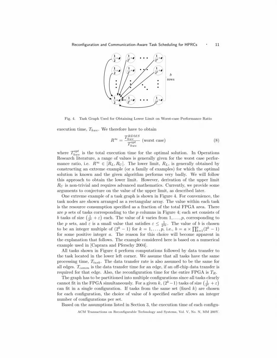
Fig. 4. Task Graph Used for Obtaining Lower Limit on Worst-case Performance Ratio

execution time, Thwe. We therefore have to obtain

R∞ =TRDMShwe

T opthwe

(worst case) (8)

where T opthwe is the total execution time for the optimal solution. In OperationsResearch literature, a range of values is generally given for the worst case perfor-mance ratio, i.e. R∞ ∈ [RL, RU ]. The lower limit, RL, is generally obtained byconstructing an extreme example (or a family of examples) for which the optimalsolution is known and the given algorithm performs very badly. We will followthis approach to obtain the lower limit. However, derivation of the upper limitRU is non-trivial and requires advanced mathematics. Currently, we provide somearguments to conjecture on the value of the upper limit, as described later.

One extreme example of a task graph is shown in Figure 4. For convenience, thetask nodes are shown arranged as a rectangular array. The value within each taskis the resource consumption specified as a fraction of the total FPGA area. Thereare p sets of tasks corresponding to the p columns in Figure 4; each set consists ofb tasks of size

(12k + ε

)each. The value of k varies from 1, . . . , p, corresponding to

the p sets, and ε is a small value that satisfies ε ≤ 122p . The value of b is chosen

to be an integer multiple of (2k − 1) for k = 1, . . . , p, i.e., b = a ×∏pk=1(2k − 1)

for some positive integer a. The reason for this choice will become apparent inthe explanation that follows. The example considered here is based on a numericalexample used in [Caprara and Pferschy 2004].

All tasks shown in Figure 4 perform computations followed by data transfer tothe task located in the lower left corner. We assume that all tasks have the sameprocessing time, Ttask. The data transfer rate is also assumed to be the same forall edges. Tcomm is the data transfer time for an edge, if an off-chip data transfer isrequired for that edge. Also, the reconfiguration time for the entire FPGA is TR.

The graph has to be partitioned into multiple configurations since all tasks clearlycannot fit in the FPGA simultaneously. For a given k, (2k−1) tasks of size

(12k + ε

)can fit in a single configuration. If tasks from the same set (fixed k) are chosenfor each configuration, the choice of value of b specified earlier allows an integernumber of configurations per set.

Based on the assumptions listed in Section 3, the execution time of each configu-ACM Transactions on Reconfigurable Technology and Systems, Vol. V, No. N, MM 200Y.


ration will be Ttask, irrespective of the number of tasks in the configuration. Sincethe data volume over each edge is the same, an optimal solution is obtained if thenumber of configurations is minimized. This corresponds to the one-dimensionalbin-packing problem (BPP) found in the literature [Coffman, Jr. et al. 1996]. Theoptimal solution is to pack p tasks, one from each set, into one bin (or configura-tion). The p tasks will fit in the configuration due to the fact that the definitionof ε guarantees

∑pk=1( 1

2k + ε) ≤ 1. The optimal solution therefore consists of bconfigurations, with the tasks in each row in Figure 4 constituting a configuration.The bottom row should naturally be configured last, due to the data dependency.The total execution time is the sum of bTR, bTtask and the total data transfer time.Since the graph has (bp − 1) edges, and off-chip data transfer is not required forthe (p − 1) edges present in the last configuration, the total data transfer time is2Tcomm[(bp−1)− (p−1)]. The factor 2 is, as explained earlier, due to data transferoccurring twice for each edge, once from FPGA to external memory and then againfrom external memory back to the FPGA. The optimal execution time is therefore,

T opthwe = b[TR + Ttask] + 2[p(b− 1)]Tcomm (9)

When RDMS schedules the same graph, it will pack the tasks differently. RDMSattempts to maximize the FPGA resource utilization for the first configuration,before proceeding with the second configuration, and so on. It is clear that RDMSwill therefore choose tasks from the last set (k = p) for the first few configurations,before proceeding with the other sets, in decreasing order of the value of k. Inother words, RDMS starts with the tasks in the last column on the right side, andproceeds toward the left in Figure 4. As mentioned earlier, only (2k − 1) tasks fromeach set can fit within a configuration. Since there are b tasks in each set, RDMSwill give b

2k−1configurations for each set. The total number of configurations is

therefore N =∑pk=1

b2k−1

. The final configuration consists of a single task, the taskpresent in the lower left corner of Figure 4. The total execution time is the sum ofNTR, NTtask and the total data transfer time. Since the graph has (bp− 1) edgesand off-chip data transfer is required for all the edges, the total data transfer timeis 2Tcomm(bp− 1). The total execution time using RDMS algorithm is therefore,

TRDMShwe = b

(p∑k=1

12k − 1

)[TR + Ttask] + 2(pb− 1)Tcomm (10)

The ratio of the execution time from (10) and (9) is

R =TRDMShwe

T opthwe

=A+ C

B +D

where A = N [TR + Ttask], C = 2(pb − 1)Tcomm, B = b[TR + Ttask] and D =2[p(b − 1)]Tcomm. Since Figure 4 depicts a family of bad examples obtained byvarying p from 1 to ∞, the ratio R differs for different instances of the family. Itcan be shown that for all the instances, A/B increases with p and asymptoticallyreaches the value 1.606695. . . (for p → ∞). Also, C/D decreases for p = 2, 3 . . .and can be shown to have an upper limit of 1.25 (corresponding to p = 2). SinceA/B ∈ [1, 1.6067) and C/D ∈ [1, 1.25], it follows that R ∈ [1, 1.6067), since R isACM Transactions on Reconfigurable Technology and Systems, Vol. V, No. N, MM 200Y.


the mediant of A/B and C/D. RL is the largest possible value of R, which is,

RL = 1.6067

It is interesting to note that the largest value of R is obtained when Tcomm = 0.This is as expected, since RDMS will perform better in the presence of data transfer(Tcomm 6= 0), because it is designed to minimize off-chip data transfer overheads.

Derivation of the upper limit RU for the worst-case ratio is difficult. However, aswe have observed for the extreme example, the worst-case performance is observedwhen the communication volume is zero. It is reasonable to extend this argumentfor all graphs, that is, RDMS will in general have the worst performance when nodata communication is present in the task graph. When the task graph has nodata communication, the problem to be solved is a BPP, and RDMS in this casebehaves identically to the subset-sum algorithm. Using detailed mathematics, ithas been shown in [Caprara and Pferschy 2004] that the subset-sum algorithm hasan upper limit worst-case performance of 1.6210. . . We therefore conjecture thatfor RDMS, RU = 1.6210. The worst-case performance ratio R∞ for the RDMSalgorithm would therefore satisfy

R∞ ∈ (1.6067, 1.6210) (11)

In general the RDMS algorithm will give a solution close to the optimum, and(11) is only a bound on the worst-case value.

4. EXPERIMENTAL RESULTS

In order to demonstrate the advantage of the proposed RDMS algorithm, we havecompared it with two other solutions that only consider hardware task resourceutilization and data dependency. One algorithm is the previous version of theRDMS algorithm, which was presented in [Huang et al. 2008] and referred to aspRDMS hereafter. The other algorithm adopts a Linear Programming Relaxation[Kellerer et al. 2004] approach, referred to as LPR. Three different comparisons aremade among the three algorithms. First, a direct comparison is carried out usingthe example graph in Figure 3(a). Second, randomly generated data flow graphsare used to cover a comprehensive scope of different applications. Third, the taskgraph from a real-life application, an astrophysics N-body simulation, is scheduledusing RDMS and pRDMS, by applying constraints from real HPRCs, the SRC-6and Cray XD1. Finally, based on the scheduling result obtained from RDMS, theN-body application is emulated on SRC-6 hardware platform and the measuredresults compared against the theoretical expectations.

4.1 Scheduling Comparison on Example Graph

The pRDMS algorithm is similar to the RDMS algorithm; however, it does notconsider the inter-task communication during the scheduling process. The pRDMSalgorithm schedules the 13 nodes of the example graph in Figure 3(a) also intofour FPGA configuration, i.e., {H2,H3,H4,H6}, {H1,H7,H9,H10,H12},{H5,H8} and{H11,H13}. A direct comparison with result from RDMS shows that RDMS reducesthe inter-configuration communication time by 21.1%.

In the LPR approach to schedule hardware tasks represented by a DAG, nodesare scheduled level by level and the nodes in the next level are not considered until



2 0 4 0 6 0 8 0 1 0 0 1 2 0 1 4 0 1 6 0 1 8 0 2 0 00

5 0 0

1 0 0 0

1 5 0 0

2 0 0 0Int

er-co

nfigu

ration

Comm

unica

tion V

olume

T a s k C o u n t

L P R p R D M S R D M S

(a) Inter-configuration Communication

2 0 4 0 6 0 8 0 1 0 0 1 2 0 1 4 0 1 6 0 1 8 0 2 0 01 0

2 0

3 0

4 0

5 0

6 0

Numb

er of

FPGA

Confi

gurat

ions

T a s k C o u n t

L P R p R D M S R D M S

(b) Number of FPGA Configurations

Fig. 5. Scheduling Efficiency Comparison Among Three Approaches When Inter-task Communi-

cation Time Is Much Smaller Than Task Configuration Time

Table I. Scheduling Efficiency Improvement on Randomly Generated Graphs Using RDMS Against

Other Two Algorithms

Inter-configuration Communication Number of Configurations

Sim 1∗ Sim 2∗ Sim 3∗ Sim 1 Sim 2 Sim 3

LPR 49.1% 39.7% 42.7% 4.3% 3.9% 4.4%

pRDMS 13.0% 7.0% 13.1% 1.8% 1.4% 1.9%

∗Sim 1: Simulation 1; Sim 2: Simulation 2; Sim 3: Simulation 3.

all nodes in the current level are scheduled. The typical LPR approach is to sortnodes in the same level into a decreasing order based on profit per weight ratio.Since the profit of each node is defined as configuration time and is linear to itsweight, all nodes have the same profit per weight ratio in our case. Therefore,all nodes in the same level are sorted in a increasing order based on weight andthen scheduled in a sequence. Once one FPGA configuration has no spare spaceto accommodate the node under consideration, it starts a new configuration. TheLPR algorithm schedules the 13 nodes of the example graph into six FPGA config-urations, i.e., {H2,H3,H4}, {H1,H6,H7}, {H5,H9,H10}, {H8}, {H11,H12}, {H13}.Correspondingly, RDMS reduces the inter-configuration communication time by63.4% compared with LPR in this case.

4.2 Scheduling Comparison on Randomly Generated Synthetic Graphs

In order to compare the scheduling efficiency among the three algorithms, i.e., LPR,pRDMS and RDMS, these algorithms have been implemented in C++. Randomlygenerated task graphs of node count from 20 to 200 were applied and the number ofconfigurations and inter-configuration communication time were recorded. For eachtask graph, there are ten nodes in each level. Every node was randomly connectedto one to three parent nodes; the weight and the configuration time of each nodeACM Transactions on Reconfigurable Technology and Systems, Vol. V, No. N, MM 200Y.


were the same and they were randomly assigned between 1 and 50. Three differentsimulations were carried out, representing three different types of systems.

(1) Simulation 1: the inter-task communication time is randomly assigned between1 and 10. In other words, the inter-task communication time is much smallerthan task configuration time. This simulation represents those RC systems thathave a long configuration time.

(2) Simulation 2: the inter-task communication time is randomly assigned between1 and 50. In other words, the inter-task communication time is comparablythe same as the task configuration time. This simulation represents those RCsystems that have a medium configuration time.

(3) Simulation 3: the inter-task communication time is randomly assigned between1 and 100. In other words, the inter-task communication time is much largerthan the task configuration time. This simulation represents those RC systemsthat have a very short configuration time.

By observing the scheduling results shown in Figure 5 and Table I, it can be seenthat the RDMS algorithm is capable of reducing the inter-configuration commu-nication time by 11% and 44% on an average, compared with pRDMS and LPRalgorithms respectively. In terms of the number of FPGA configurations, the RDMSalgorithm generates on average, 2% and 4% less configurations than pRDMS andLPR respectively.

4.3 Astrophysics N-Body Simulation

4.3.1 Application Description. The target application we intend to implementon a reconfigurable computer is part of an astrophysical N-Body simulations wheregas-dynamical effects are treated by a smoothed particle hydrodynamics (SPH)method [Lucy 1977; Monaghan and Lattanzio 1985; Lienhart et al. 2002]. Theprinciple of this method is that the gaseous matter is represented by particles,which have a position, velocity and mass. In order to form a continuous distribu-tion of gas from these particles, they are smoothed by folding their discrete massdistribution with a smoothing kernel W . This folding means that the point massesof the particles become smeared so that they form a density distribution. At agiven position the density is calculated by summing the smoothed densities of thesurrounding particles. Mathematically, the summation can be written as

ρi =N∑j=1

mjW (~ri − ~rj , h) (12)

where h is the smoothing length specifying the radius of the summation space.Commonly used smoothing kernels are strongly peaked functions around zero and

are non-zero only in a limited area. A natural choice for the kernel is the spher-ically symmetric spline kernel proposed by Monaghan and Lattanzio [Monaghan



#1Difference Vectorvij_x = vi_x – vj_x vij_y = vi_y – vj_yvij_z = vi_z – vj_z

#2Difference Vectorrij_x = ri_x – rj_x rij_y = ri_y – rj_yrij_z = ri_z – rj_z

#3Mean Value

hij = (hi + hj) / 2

#5Mean Value

cij = (ci + cj) / 2

#6Mean Value

rhoij = (rhoi + rhoj) / 2

#4Mean Valuefij = (fi + fj) / 2

#7p/rho2

prhoi2 = pi / (rhoi × rhoi) orprhoj2 = pj / (rhoj × rhoj)

#8Scalarprod

vrij = (vij_x × rij_x) + (vij_y × rij_y) + (vij_z × rij_z)

#9Scalarprod

rij2 = (rij_x × rij_x) + (rij_y × rij_y) + (rij_z × rij_z)

#11muij

muij = hij × vrij × fij / (rij2 + eta × hij × hij)

#12Squarerootrij = sqrt rij2

#10ihij = 1 / hij

#13ihij5 = ihij^5

#15piij

if vrij > 0 thenpiij = 0

elsepiij = (-alpha × cij × muij +

beta × muij × muij) / rhoij

#14rh = rij × ihij

#16Gradient of W

if 0 < rh ≤ 1 thendW = (9 × rh / 4 - 3) × ihij5

else if 1 < rh ≤ 2 thendW = (-3 × rh /4 + 3 – 3 / rh) × ihij5

elsedW = 0

#17Scalar Factor dvs

dvs = mj × (prhoi2 + prhoj2 + piij) × dW

#18Build dv vector

dv_x = dv_x + rij_x × dvsdv_y = dv_y + rij_y × dvsdv_z = dv_z + rij_z × dvs

Input Datari_x, ri_y, ri_z, rj_x, rj_y, rj_z,

vi_x, vi_y, vi_z, vj_x, vj_y, vj_z, hi, hj, fi, fj, ci, cj, pi, pj, rhoi, rhoj,

mj

prhoi288

1688

24 248 8

8 8 8

8

24

88

8

8

8

24 24

24 8

8Inter-task communication

volume in byte for processing one neighbor particle

8

8

8

8

8

8

8

Fig. 6. Data Flow Graph of SPH Pressure Force Calculation (with Assigned Node Number in

Each Box)

and Lattanzio 1985], defined by

W (~ri − ~rj , h) =1h3B

(x =

|~ri − ~rj |h

)

with B(x) =

1− 3

2x2 + 3

4x3 0 < x ≤ 1

14 (2− x)3 1 < x ≤ 20 x > 2

(13)

The important point of SPH is that any gas-dynamical variables and even theirderivatives can be calculated by a simple summation over the particle data multi-plied by the smoothing kernel or its derivative. The motion of the SPH particles isdetermined by the gas-dynamical force calculated via the smoothing method, andthe particles move as Newtonian point masses under this force. Equation 14 is thephysical formulation of the velocity derivative given by the pressure force and theartificial viscosity.ACM Transactions on Reconfigurable Technology and Systems, Vol. V, No. N, MM 200Y.


d~vidt

= − 1ρi∇Pi + ~avisci (14)

The SPH method transforms Equation (14) to the formulation in Equation (15),which is only one of several possibilities.

d~vidt

= −N∑j=1

mj(piρ2i

+pjρ2j

+ Πij)∇iW (~rij , hij)

Πij =

{−αcijµij+βµ2ij

ρij~vij~rij ≤ 0

0 ~vij~rij > 0

~rij = ~ri − ~rj , ~vij = ~vi − ~vj , ρij =ρi + ρj

2

fij =fi + fj

2, cij =

ci + cj2

, hij =hi + hj

2

µij =hij~vij~rij~r2ij + η2h2

ij

fij

(15)

The gradient of W in Equation (15) consists of three components in Cartesiancoordinates (x, y, z). The x-component of the gradient of the smoothing kernel isshown in Equation (16). The calculation of y and z-components is the same.

∂iW

∂x=

( 9|~rij |

4h6ij− 3

h5ij

)(rix − rjx) 0 < |~rij |hij≤ 1

(− 3|~rij |4h6

ij+ 3

h5ij− 3

h4ij |~rij | )(rix − rjx) 1 < |~rij |

hij≤ 2

0 |~rij |hij

> 2

(16)

The diagram in Figure 6 shows the data flow to compute Equation (15), whichconsists of a total of 18 tasks. The communication volume of the edges in Figure 6is based on the task requirements, obtained using the equations describing eachtask. For example, task #1 uses six double precision variables as inputs; three ofthese variables, viz., vi x, vi y, and vi z, need to be transferred only once whencalculating the SPH pressure force for particle i. Therefore only three variables,corresponding to the neighbor particles, are shown as inputs to task #1. The inputedge to task #1 is therefore shown to carry 24 bytes.

4.3.2 Testbeds. To obtain realistic performance estimates for the SPH pressureforce calculation pipeline, we have used the system parameters from two existingHPRC platforms, the SRC-6 and Cray XD1. The whole FPGA configuration timeis 130 ms on SRC-6 and 1,824 ms on Cray XD1, respectively. On both platforms,the bandwidth of interconnect is 1.4×109 B/s.

RDMS and pRDMS algorithm are used for scheduling the graph given in Fig-ure 6. LPR results are not considered here, since the previous subsection clearlydemonstrates that RDMS and pRDMS outperform LPR by a large margin. Inorder to get desired performance and computation accuracy for the graph in Fig-ure 6, fully pipelined double-precision (64-bit) floating point arithmetic units are



Table II. Resource Utilization of Pipelined Double-precision (64-bit) Floating-point Operators

+/− × ÷ √

Slices 1,640∗ 2,085∗ 4,173∗ 2,700∗

∗+/−: [Govindu et al. 2005], ×: [Zhuo and Prasanna 2007],÷: [Hemmert and Underwood 2006],

√: [Thakkar and Ejnioui 2006]

Table III. Resource Utilization of Hardware TasksNode Operator∗

SlicesPercentage of Device Utilization†

No. Combination XC2V6000 XC2VP50

1,2 3A 4,920 17.13 24.51

3,4,5,6 1A 1,640 5.71 8.17

7 1M,1D 6,258 21.79 31.17

8,9 2A,3M 9,535 33.20 47.50

10 1D 4,173 14.53 20.79

11,15 1A,4M,1D 14,153 49.27 70.50

12 1S 2,700 9.40 13.45

13 4M 8,340 29.04 41.55

14 1M 2,085 7.26 10.39

16 3A,4M,1D 17,433 60.69 86.84

17 2A,2M 7,450 25.94 37.11

18 3A,3M 11,175 38.91 55.67

Overall 24A,29M,5D,1S 123,390 429.59 614.68

∗A: adder/subtractor, M: multiplier, D: divider, S: square root.†Assume 15% of slices in device are reserved for vendor service logic.

needed for implementation on hardware. Many researchers have reported variousfloating-point arithmetic designs on FPGA devices [Govindu et al. 2005; Zhuo andPrasanna 2007; Hemmert and Underwood 2006; Thakkar and Ejnioui 2006]. Theresource utilization of pipelined double-precision (64-bit) floating-point operatorsbased on available literature is listed in Table II. These primitive operators are usedto construct the functionality of nodes in Figure 6. In general, multiple primitiveoperators are used to build a pipelined hardware node so that all operations in oneFPGA configuration can be executed in parallel to maximize the throughput. Forinstance, node #11 needs 1 adder, 4 multipliers and 1 divider, which is denoted as“1A,4M,1D” in Table III. The amount of slices occupied by each node is simplythe summation of the slices of the primitive operators. We list the percentage ofslice utilization of each node on the FPGA devices of the two representative recon-figurable computers in Table III, i.e., Virtex-II6000 with SRC-6 and Virtex-IIP50with Cray XD1. It is evident that multiple FPGA configurations are required toimplement the dataflow graph in Figure 6 on both platforms.



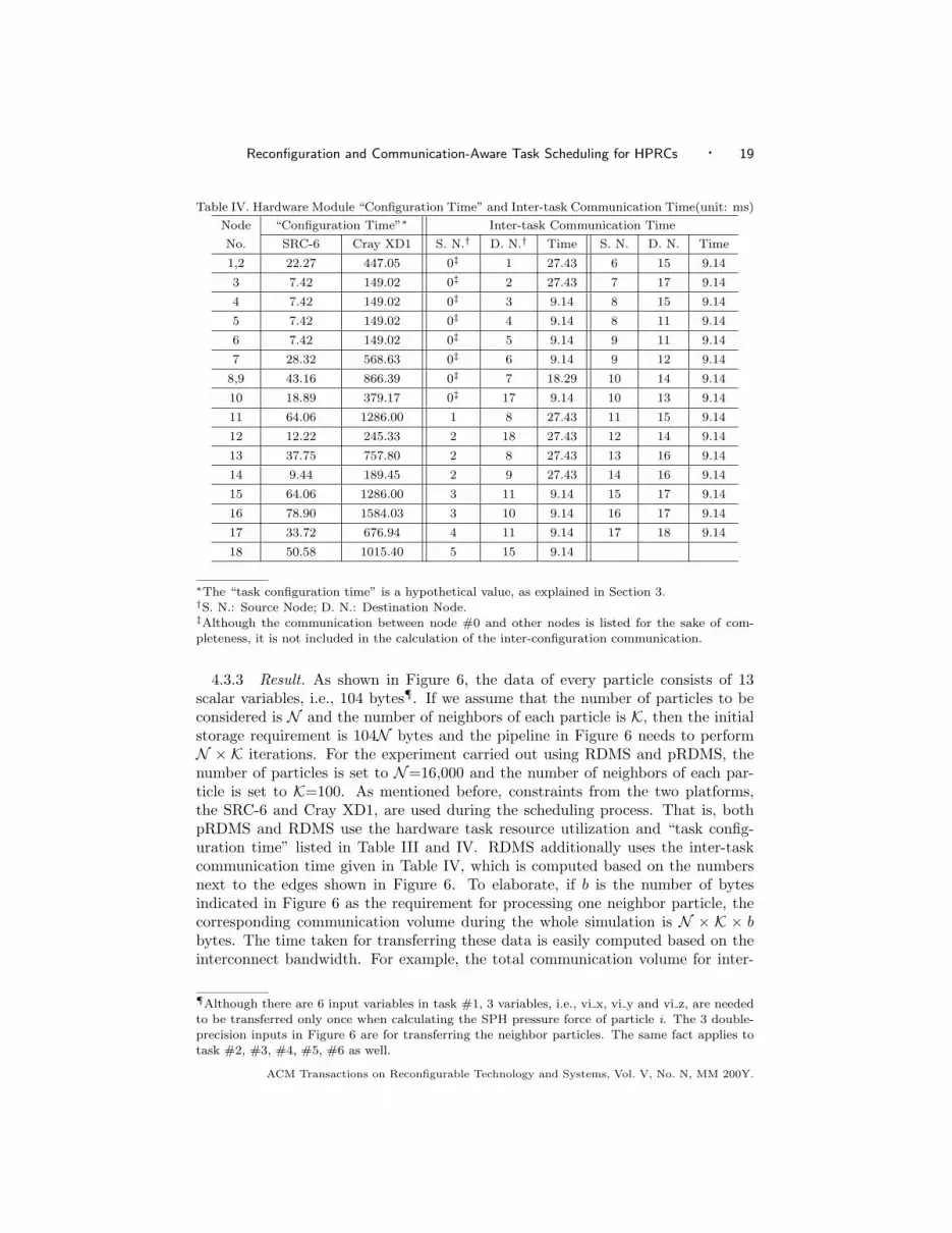
Table IV. Hardware Module “Configuration Time” and Inter-task Communication Time(unit: ms)

Node “Configuration Time”∗ Inter-task Communication Time

No. SRC-6 Cray XD1 S. N.† D. N.† Time S. N. D. N. Time

1,2 22.27 447.05 0‡ 1 27.43 6 15 9.14

3 7.42 149.02 0‡ 2 27.43 7 17 9.14

4 7.42 149.02 0‡ 3 9.14 8 15 9.14

5 7.42 149.02 0‡ 4 9.14 8 11 9.14

6 7.42 149.02 0‡ 5 9.14 9 11 9.14

7 28.32 568.63 0‡ 6 9.14 9 12 9.14

8,9 43.16 866.39 0‡ 7 18.29 10 14 9.14

10 18.89 379.17 0‡ 17 9.14 10 13 9.14

11 64.06 1286.00 1 8 27.43 11 15 9.14

12 12.22 245.33 2 18 27.43 12 14 9.14

13 37.75 757.80 2 8 27.43 13 16 9.14

14 9.44 189.45 2 9 27.43 14 16 9.14

15 64.06 1286.00 3 11 9.14 15 17 9.14

16 78.90 1584.03 3 10 9.14 16 17 9.14

17 33.72 676.94 4 11 9.14 17 18 9.14

18 50.58 1015.40 5 15 9.14

∗The “task configuration time” is a hypothetical value, as explained in Section 3.†S. N.: Source Node; D. N.: Destination Node.‡Although the communication between node #0 and other nodes is listed for the sake of com-

pleteness, it is not included in the calculation of the inter-configuration communication.

4.3.3 Result. As shown in Figure 6, the data of every particle consists of 13scalar variables, i.e., 104 bytes¶. If we assume that the number of particles to beconsidered is N and the number of neighbors of each particle is K, then the initialstorage requirement is 104N bytes and the pipeline in Figure 6 needs to performN × K iterations. For the experiment carried out using RDMS and pRDMS, thenumber of particles is set to N=16,000 and the number of neighbors of each par-ticle is set to K=100. As mentioned before, constraints from the two platforms,the SRC-6 and Cray XD1, are used during the scheduling process. That is, bothpRDMS and RDMS use the hardware task resource utilization and “task config-uration time” listed in Table III and IV. RDMS additionally uses the inter-taskcommunication time given in Table IV, which is computed based on the numbersnext to the edges shown in Figure 6. To elaborate, if b is the number of bytesindicated in Figure 6 as the requirement for processing one neighbor particle, thecorresponding communication volume during the whole simulation is N × K × bbytes. The time taken for transferring these data is easily computed based on theinterconnect bandwidth. For example, the total communication volume for inter-

¶Although there are 6 input variables in task #1, 3 variables, i.e., vi x, vi y and vi z, are needed

to be transferred only once when calculating the SPH pressure force of particle i. The 3 double-precision inputs in Figure 6 are for transferring the neighbor particles. The same fact applies to

task #2, #3, #4, #5, #6 as well.



Table V. SPH Pressure Force Scheduling Efficiency Comparison between pRDMS and RDMS

pRDMS RDMS

Inter-configuration SRC-6 0.347 0.329

Communication Time (s) Cray XD1 0.512 0.384

Number of FPGA SRC-6 5∗ 5†

Configurations Cray XD1 7‡ 7§

∗{1,2,6,7,8}, {3,4,5,9,10,13}, {11,15}, {12,14,16}, {17,18}.†{1,2,6,7,8}, {3,4,5,9,10,12,14}, {11,15}, {13,16}, {17,18}, see Table VI for detail.‡{1,2,3,4,7}, {8,9}, {6,11,12}, {5,10,13,14}, {16}, {15}, {17,18}.§{1,2,8}, {5,6,7,9}, {3,4,10,12,13}, {14,16}, {11}, {15}, {17,18}.

task communication between task #2 and #8 is 16, 000 × 100 × 24 = 3.84 × 107

bytes, which will need 27.43 ms for transfer over an I/O with bandwidth 1.4× 109

B/s.The number of FPGA configurations and the inter-configuration communication

time, obtained from the scheduling algorithms for both platforms, are listed in Ta-ble V. The inter-configuration communication time is obtained by summing upthe I/O time for all configurations. For example, the fourth configuration obtainedusing RDMS for SRC-6 consists of the tasks #13 and #16. From Figure 6, thisconfiguration would require two inputs (8 bytes each) and one output (8 bytes),or collectively 24 bytes per neighbor particle. These 24 bytes corresponds to atotal I/O transfer time of 27.43 ms using a 1.4 GB/s interconnect, as shown ear-lier. Similar computations are carried out for all configurations. To illustrate theactual numbers obtained for one case (RDMS for SRC-6), the values for all theinter-configuration communications are listed in Table VI under the column la-beled ‘Estimated (using 1.4GB/s)’. The procedure outlined here is carried out forRDMS as well as pRDMS, using the parameters for the two platforms.

Based on the scheduling results, the following observations can be made. Onthe SRC-6 platform, RDMS reduces the communication time by 5% compared topRDMS. An analysis of both scheduling sequences has shown that pRDMS has elim-inated some high volume data communication simply because they belong to thefirst tasks that were combined. For example, RDMS has scheduled task #9, #10,#12 and #14 into the same configuration whereas pRDMS has scheduled them intotwo separate configurations, which increases the overall inter-configuration commu-nication. On Cray XD1, the communication reduction is increased to 25% sinceRDMS successfully schedules those tasks between which there exists heavy commu-nications into the same configuration, e.g., #1, #2 and #8. The communicationreduction is higher because Cray XD1 uses smaller FPGAs and therefore it is lesslikely that high volume communication transfers are covered by pRDMS. To sum-marize, RDMS algorithm is effective in reducing the communication overhead for areal-life application like the N-body simulation, in addition to reducing the numberof configurations.

4.3.4 Experiments on Hardware and Discussion of the Limitations. In order todemonstrate the applicability of the proposed algorithm, and also to understandits limitations, we have emulated the execution of the N-body application on theACM Transactions on Reconfigurable Technology and Systems, Vol. V, No. N, MM 200Y.


Table VI. The RDMS Implementation of SPH Pressure Force on the SRC-6

Tasks

Inter-Configuration Communication Time (ms)

FPGA Estimated Estimated Measured

Configuration (using 1.4 GB/s) (using 800 MB/s)

Input Output Input Output Input Output

1 1,2,6,7,8 0 91.42 0 159.99 0 163.55

2 3,4,5,9,10,12,14 27.43 54.84 48.00 95.97 48.13 98.35

3 11,15 63.98 9.14 111.97 16.00 112.30 16.31

4 13,16 18.28 9.14 31.99 16.00 32.10 16.30

5 17,18 54.85 0 95.99 0 96.26 0

Total 164.54 164.54 287.95 287.95 288.79 294.51

SRC-6 platform. The task graph for N-body simulation is first scheduled usingRDMS, to determine the constituent configurations as described in the previoussubsection. We have observed that the practically achieved interconnect bandwidthon the SRC-6 is 800 MB/s as against the theoretically achievable 1.4 GB/s, whenthe amount of data per transaction is comparably small, say 4 MB. This practicalvalue is used in obtaining the scheduling result. It turns out that the tasks in eachconfiguration, with this reduced interconnect bandwidth, is the same as that listedin the footnote of Table V.

After obtaining the schedule, the execution of the application is emulated onhardware. To be specific, in the absence of double-precision floating point imple-mentations for the constituent tasks of N-body simulation, we have emulated theexecution of each task by simple delays. Rather than checking the functionality ofthe application, the purpose of this experiment is to verify the proposed approachbased on actual data transfers and in the presence of reconfiguration of the FPGA.

Table VI shows the measured results from the experiments on SRC-6, comparedagainst the theoretically expected results. The results show that the theoreticalexpectations are very close to the experimentally measured results. This clearlydemonstrates the applicability of the proposed algorithm.

The scheduling results and experiments reveal some of the limitations of theRDMS algorithm. For instance, the RDMS algorithm does not try to reuse sharededges in a task graph. As an example, consider tasks #11 and #15 in Figure 6,which comprise the third configuration scheduled by RDMS. Both of these tasksuse the same output from task #8, yet the same data is transferred separately forthe two tasks even though they reside in the same configuration. This is reflectedin the task communication time (measured and expected values) listed in Table VI.

The RDMS algorithm also does not consider limitations of bandwidth of locallyattached memory. While this assumption is accurate when internal block RAMof the FPGA is used, there could be some limitations in the presence of externallocal memory. As an example, consider again the configuration 3, which consistsof tasks #11 and #15. From the numbered edges in Figure 6, it can be deducedthat during execution, this configuration requires 7 input ports and 1 output portto access local memory, with each port having a width of 8 bytes (or 64-bits). Thisrequirement cannot be directly satisfied in the SRC-6, since it features only 6 local



SRAM modules attached to one FPGA. The FPGA in the SRC-6 therefore hasaccess to only 6 ports of 64-bits each. Sharing of this limited bandwidth for thetasks would result in a degradation of the task execution time. Detailed executionof the tasks is currently not modeled in our emulation experiments.

It is also worth mentioning that RDMS currently works only for the cases whenthe data processed is very large, thereby allowing us to ignore pipeline latencies.Tasks within a configuration are therefore considered to execute in parallel. Furtherresearch is needed to extend RDMS for the cases when smaller data is processed,as well as when task execution is not carried out in a pipelined fashion (i.e., taskswithin a configuration execute one after the other). Additional considerations in-clude limitations in the size of local memory attached to the FPGA. One possiblesolution to this problem is to use multiple installments of input and output datatransfer, interleaved with execution. The other alternative is to reconfigure theFPGA several times for the same sequence of configurations, with each sequenceoperating only on a part of the data (so I/O transfer occurs only for the firstand last configuration of one sequence of configurations). There will definitely betradeoffs between choosing multiple configuration sequences (with reduced datatransfers) versus multiple data installments (and fewer configuration sequences);further study is required to analyze these tradeoffs.

5. CONCLUSIONS

In this paper, we have proposed the Reduced Data Movement Scheduling (RDMS)algorithm, for scheduling tasks assigned to FPGA co-processors on RC systems.RDMS reduces the inter-configuration communication overhead and FPGA con-figuration overhead by taking data dependency, hardware task resource utilizationand inter-task communication into account during the scheduling process. Mathe-matical analysis of the algorithm shows that the time complexity is O(n3W 2) in theworst-case, and the maximum space requirement is O(n(n+W )), for a graph withn nodes. These are reasonable requirements for a static task scheduling algorithm.The worst-case performance ratio of RDMS is expected to have a value between1.6067 and 1.6210, which is good for a heuristic scheduler that takes into accountmany constraints. Simulation results show that the RDMS algorithm is able to re-duce inter-configuration communication time by 11% and 44% respectively and alsogenerate fewer FPGA configurations, compared to pRDMS and LPR algorithms,which only consider data dependency and task resource utilization during schedul-ing. The scheduling results obtained for a real-life application, N-body simulation,for SRC-6 and Cray XD1 platforms, verifies the efficiency of RDMS algorithm.Experiments on SRC-6 further validate the proposed approach.

ACKNOWLEDGMENTS

This work was supported in part by the I/UCRC Program of the National Sci-ence Foundation under Grant No. IIP-0706352. The authors thank the anonymousreviewers for their comments that greatly helped in improving the quality of thepaper. The authors are grateful to Dr. Mohamed Bakhouya for helpful discussions.The authors would like to thank Guillermo Marcus from Institute for Computer En-gineering of the University of Heidelberg in Germany for helpful discussions aboutACM Transactions on Reconfigurable Technology and Systems, Vol. V, No. N, MM 200Y.


N-body simulation using FPGAs. The authors also would like to acknowledge Ger-hard Lienhart, Andreas Kugel and Reinhard Manner from University of Mannheimin Germany for providing the data flow graph of SPH pressure force calculation.

REFERENCES

Bazargan, K., Kastner, R., and Sarrafzadeh, M. 2000. Fast template placement for recon-figurable computing systems. IEEE Design and Test of Computers 17, 1 (Jan.), 68–83.

Brebner, G. and Diessel, O. 2001. Chip-based reconfigurable task management. In Proc.International Conference on Field Programmable Logic and Applications, 2001 (FPL 2001).

182–191.

Caprara, A. and Pferschy, U. 2004. Worst-case analysis of the subset sum algorithm for bin

packing. Operations Research Letters 32, 2 (Mar.), 159–166.

Coffman, Jr., E. G., Garey, M. R., and Johnson, D. S. 1996. Approximation algorithms for

bin packing: a survey. In Approximation Algorithms for NP-Hard Problems, D. Hochbaum

(ed.), PWS Publishing, Boston. 46–93.

Compton, K., Li, Z., Cooley, J., Knol, S., and Hauck, S. 2002. Configuration relocation and

defragmentation for run-time reconfigurable computing. IEEE Trans. VLSI Syst. 10, 3 (June),209–220.

Diessel, O., ElGindy, H., Middendorf, M., Schmeck, H., and Schmidt, B. 2000. Dynamicscheduling of tasks on partially reconfigurable fpgas. IEE Proceedings - Computers and Digital

Techniques, Special Issue on Reconfigurable Systems 147, 3 (May), 181–188.

Fekete, S. P., Kohler, E., and Teich, J. 2001. Optimal FPGA module placement with temporal

precedence constraints. In Proc. Design, Automation and Test in Europe Conference and

Exhibition, 2001 (DATE’01). 658–665.

Govindu, G., Scrofano, R., and Prasanna, V. K. 2005. A library of parameterizable floating-

point cores for FPGAs and their application to scientific computing. In Proc. The InternationalConference on Engineering Reconfigurable Systems and Algorithms (ERSA’05). 137–145.

Handa, M. and Vemuri, R. 2004. A fast algorithm for finding maximal empty rectangles fordynamic FPGA placement. In Proc. Design, Automation and Test in Europe Conference and

Exhibition, 2004 (DATE’04). Vol. 1. 744–745.

Hemmert, K. S. and Underwood, K. D. 2006. Open source high performance floating-point

modules. In Proc. the 14th Annual IEEE Symposium on Field-Programmable Custom Com-

puting Machines (FCCM’06). 349–350.

Huang, M., Simmler, H., Saha, P., and El-Ghazawi, T. 2008. Hardware task scheduling

optimizations for reconfigurable computing. In Proc. Second International Workshop on High-Performance Reconfigurable Computing Technology and Applications (HPRCTA’08).

Huang, M., Simmler, H., Serres, O., and El-Ghazawi, T. 2009. RDMS: A hardware taskscheduling algorithm for reconfigurable computing. In Proc. the 16th Reconfigurable Architec-

tures Workshop (RAW 2009).

Kellerer, H., Pferschy, U., and Pisinger, D. 2004. Knapsack problems. Springer, Berlin;

New York.

Kleinberg, J. and Tardos, E. 2005. Algorithm Design. Pearson/Addison-Wesley, Boston, MA.

Lienhart, G., Kugel, A., and Manner, R. 2002. Using floating-point arithmetic on FPGAsto accelerate scientific N-body simulations. In Proc. the 10th Annual IEEE Symposium on

Field-Programmable Custom Computing Machines (FCCM’02). 182–191.

Lucy, L. B. 1977. A numerical approach to the testing of the fission hypothesis. The AstronomicalJournal 82, 12 (Dec.), 1013–1024.

Monaghan, J. J. and Lattanzio, J. C. 1985. A refined particle method for astrophysical prob-

lems. Astronomy and Astrophysics 149, 135–143.

Pisinger, D. 1999. Linear time algorithms for knapsack problems with bounded weights. Journal

of Algorithms 33, 1 (Oct.), 1–14.



Saha, P. 2007. Automatic software hardware co-design for reconfigurable computing systems.

In Proc. International Conference on Field Programmable Logic and Applications, 2007 (FPL2007). 507–508.

Thakkar, A. J. and Ejnioui, A. 2006. Design and implementation of double precision floating

point division and square root on FPGAs. In Proc. IEEE Aerospace 2006.

Walder, H. and Platzner, M. 2002. Non-preemptive multitasking on fpga: Task placement andfootprint transform. In Proc. the 2nd International Conference on Engineering of Reconfig-

urable Systems and Architectures (ERSA). 24–30.

Walder, H., Steiger, C., and Platzner, M. 2003. Fast online task placement on FPGAs:

free space partitioning and 2D-hashing. In Proc. IEEE International Parallel and DistributedProcessing Symposium, 2003 (IPDPS’03). 178–185.

Wiangtong, T., Cheung, P., and Luk, W. 2003. Multitasking in hardware-software codesign for

reconfigurable computer. In Proc. the 2003 International Symposium on Circuits and Systems,(ISCAS ’03). Vol. 5. 621–624.

Zhuo, L. and Prasanna, V. K. 2007. Scalable and modular algorithms for floating-point matrix

multiplication on reconfigurable computing systems. IEEE Trans. Parallel Distrib. Syst. 18, 4

(Apr.), 433–448.

Received March 2009; revised July 2009; accepted August 2009


reconfiguration and communication-aware task scheduling for high-performance reconfigurable...

Documents