1

Continuity Aspects of EmbeddedReconfigurable Computing

Phan Cong Vinh and Jonathan P. Bowen

London South Bank UniversityCentre for Applied Formal Methods, Institute for Computing Research

Faculty of BCIM, Borough Road, London SE1 0AA, UK

URL: http://www.cafm.lsbu.ac.uk/Email: {phanvc,bowenjp}@lsbu.ac.uk

Abstract— In embedded systems, dynamically reconfigurablecomputing can be partially modified at runtime without stoppingthe operation of the whole system. In this paper, we consider areorganization mechanism for dynamically reconfigurable com-puting in embedded systems to guarantee that invariants of thedesign are respected. This reorganization is considered as a visualtransformation of the logical configuration by the formulatedrules. The invariant is recognized under the restructuring of theconfiguration using reconfiguration rules.

Index Terms— Dynamic reconfiguration; Embedded systems;Formal methods; Reconfigurable computing; Software develop-ment

I. I NTRODUCTION

Fast runtime partial reconfiguration features of embeddedsystems [9], [11] are available for programming the conceptof dynamically reconfigurable computing by on-the-fly reor-ganizing of available cells in regular array structures such asthose in FPGAs (Field-Programmable Gate Arrays). This isnot only relevant to the composition of new embedded systemsusing architectures and procedural models that stem from the“designed for change” methodology but also can be of decisiveimportance during the perpetual process of upgrading existingevolution-capable embedded systems.

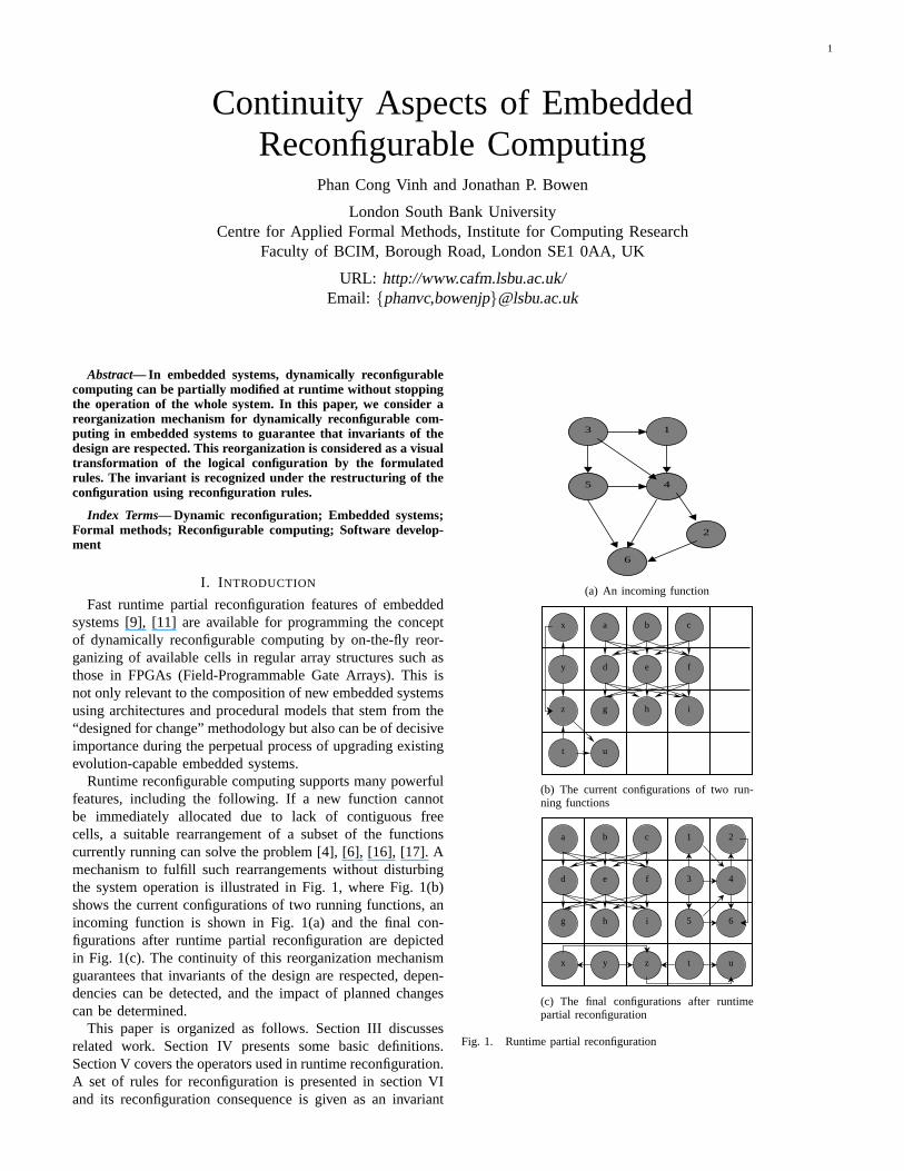
Runtime reconfigurable computing supports many powerfulfeatures, including the following. If a new function cannotbe immediately allocated due to lack of contiguous freecells, a suitable rearrangement of a subset of the functionscurrently running can solve the problem [4], [6], [16], [17]. Amechanism to fulfill such rearrangements without disturbingthe system operation is illustrated in Fig. 1, where Fig. 1(b)shows the current configurations of two running functions, anincoming function is shown in Fig. 1(a) and the final con-figurations after runtime partial reconfiguration are depictedin Fig. 1(c). The continuity of this reorganization mechanismguarantees that invariants of the design are respected, depen-dencies can be detected, and the impact of planned changescan be determined.

This paper is organized as follows. Section III discussesrelated work. Section IV presents some basic definitions.Section V covers the operators used in runtime reconfiguration.A set of rules for reconfiguration is presented in section VIand its reconfiguration consequence is given as an invariant

3 1

5 4

2

6

(a) An incoming function

b c a

e d f

g h i

u t

z

y

x

(b) The current configurations of two run-ning functions

b c a

e d f

g h i

1

4

2

6

3

5

u x y z t

(c) The final configurations after runtimepartial reconfiguration

Fig. 1. Runtime partial reconfiguration

2

in section VII. Some algorithms for the reconfiguration aredeveloped in sections VIII and IX. Finally, a short conclusionis given in section X.

II. M OTIVATION

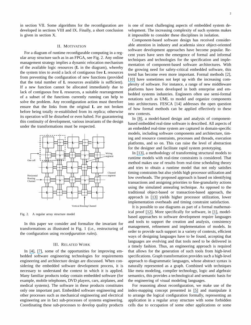
For a diagram of runtime reconfigurable computing in a reg-ular array structure such as in an FPGA, see Fig. 2. Any onlinemanagement strategy implies a dynamic relocation mechanismof the available logic resources (L in the diagram), wherebythe system tries to avoid a lack of contiguous freeL resourcesfrom preventing the configuration of new functions (providedthat the total number ofL resources available is sufficient).If a new function cannot be allocated immediately due tolack of contiguous freeL resources, a suitable rearrangementof a subset of the functions currently running can help tosolve the problem. Any reconfiguration action must thereforeensure that the links from the originalL are not brokenbefore being totally re-established from its replica; otherwiseits operation will be disturbed or even halted. For guaranteeingthis continuity of development, various invariants of the designunder the transformations must be respected.

Channel segment

Wiring segment

Vertical Routing Channel

Horizontal Routing Channel

One cell

c s

c

c s

c

c

c

c s

c

c s

c

L c c L L

L L

L L L

L

Fig. 2. A regular array structure model

In this paper we consider and formalize the invariant fortransformations as illustrated in Fig. 1 (i.e., restructuring ofthe configuration usingreconfiguration rules).

III. R ELATED WORK

In [4], [7], some of the opportunities for improving em-bedded software engineering technologies for requirementsengineering and architecture design are discussed. When con-sidering the embedded software development process, it isnecessary to understand the context in which it is applied.Many familiar products today contain embedded software (forexample, mobile telephones, DVD players, cars, airplanes, andmedical systems). The software in these products constitutesonly one important part. Embedded software engineering andother processes such as mechanical engineering and electricalengineering are in fact sub-processes of systems engineering.Coordinating these sub-processes to develop quality products

is one of most challenging aspects of embedded system de-velopment. The increasing complexity of such systems makesit impossible to consider these disciplines in isolation.

Component-based software design has received consider-able attention in industry and academia since object-orientedsoftware development approaches have become popular. Re-cent years have seen the emergence of formal and informaltechniques and technologies for the specification and imple-mentation of component-based software architectures. Withthe growing need for safety-critical embedded software, thistrend has become even more important. Formal methods [2],[10] have sometimes not kept up with the increasing com-plexity of software. For instance, a range of new middlewareplatforms have been developed in both enterprise and em-bedded systems industries. Engineers often use semi-formalnotations such as UML to model and organize componentsinto architectures. FESCA [14] addresses the open questionof how formal methods can be applied effectively to thesenew contexts.

In [8], a model-based design and analysis of component-based embedded real-time software is described. All aspects ofan embedded real-time system are captured in domain-specificmodels, including software components and architecture, tim-ing and resource constraints, processes and threads, executionplatforms, and so on. This can raise the level of abstractionfor the designer and facilitate rapid system prototyping.

In [13], a methodology of transforming structural models toruntime models with real-time constraints is considered. Thatmethod makes use of results from real-time scheduling theoryand tries to obtain a runtime model that not only satisfiestiming constraints but also yields high processor utilization andlow overheads. The proposed approach is based on identifyingtransactions and assigning priorities to fine-granularity actionsusing the simulated annealing technique. As opposed to thetraditional object-based or transaction-based approach, theapproach in [13] yields higher processor utilization, lowerimplementation overheads and timing constraint satisfaction.

It is possible to use diagrams as part of a formal mathemat-ical proof [12]. More specifically for software, in [1], model-based approaches to software development require languagesand tools to support the creation and analysis, consistencymanagement, refinement and implementation of models. Inorder to provide such support in a variety of contexts, efficientways of designing languages have to be found, accepting thatlanguages are evolving and that tools need to be delivered ina timely fashion. Thus, an engineering approach is requiredthat allows for the generation of such tools from high-levelspecifications. Graph transformation provides such a high-levelapproach to diagrammatic languages, whose abstract syntax isnaturally represented as a graph. Combined with techniqueslike meta modeling, compiler technology, logic and algebraicsemantics, this provides a technological and semantic basis forthe engineering of visual modeling languages.

For reasoning about reconfiguration, we make use of theindex-mapping concept presented in [5] and manipulate itto arrange the logical configuration formally, representing anapplication in a regular array structure with some forbiddencells due to occupation of some other applications or some

3

fault. The basic definitions in section IV are inspired bythe index-mapping concept. Significantly, our rules of recon-figuration are be built from these concepts; the invariant isrecognized under the restructure of configuration using therules and our heuristic approach to dynamical reconfigurationis formally developed. By applying this heuristic, the problemof reconfiguring a running application dynamically is solved.

IV. SOME BASIC DEFINITIONS

Definition 4.1: Logical configurationA logical configurationis a set oflogical indexpairs(x, y) 6=(0, 0) of the abstract cells of regular array structure, namelyworking cells. In other words, a pair of logical indexes denotesthe function performed by a working cell in the logicalconfiguration. Anynon-working cell, namelyunused cellorspare, has its logical indexes set to(0, 0).

The whole logical configuration is associated with an arrayL of logical indexes. Fig. 3 shows a regular array structure of4× 4 cells with two unused rows and two unused columns.

(0,0) (0,0) (0,0) (0,0) (0,0) (0,0) (0,0) (1,1) (1,2) (1,3) (1,4) (0,0) (0,0) (2,1) (2,2) (2,3) (2,4) (0,0) (0,0) (3,1) (3,2) (3,3) (3,4) (0,0) (0,0) (4,1) (4,2) (4,3) (4,4) (0,0) (0,0) (0,0) (0,0) (0,0) (0,0) (0,0)

Fig. 3. A 4× 4 array with the unused cells having(0, 0) logical indexes

Definition 4.2: ReconfigurationReconfigurationis as a transformation of the logical configu-ration by the reconfiguration rules.

Note that, hereby, the meaning ofreconfigurationandcon-figuration transformationare similar and they are exchange-able in use.

Definition 4.3: LocalityLocality in reconfiguration is the predetermined bounds allow-ing each pair of logical indexes to be only transformed ontoa restricted set of cells at limited distance from the currentnominal position.

The locality in reconfiguration is expressed by the adjacencydomain notion.

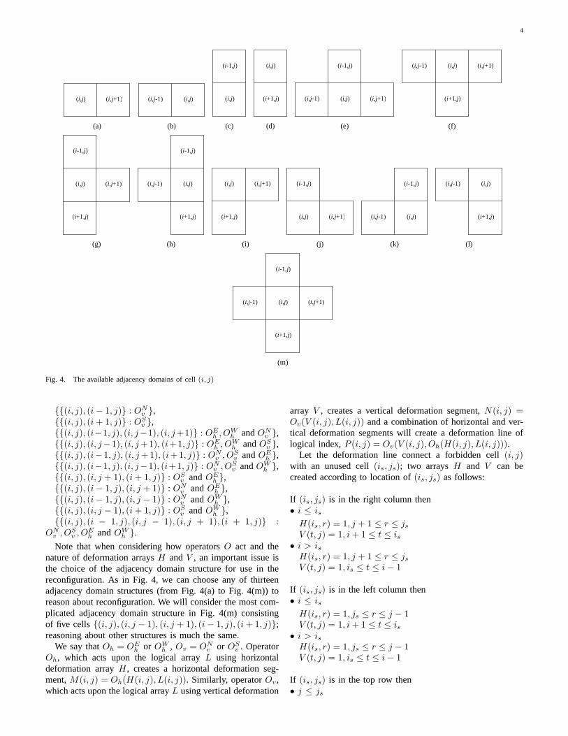
Definition 4.4: Adjacency domainAn adjacency domainof cell (i, j) consists of precisely allcells onto which the logical index(i, j) can be transformed asa consequence of reconfiguration.

Note that there are several available structures of adjacencydomain based on this definition so we can choose one kindfor reconfiguration. The number of rows and columns relatedto the directions and structure of the adjacency domains areillustrated in Fig. 4. For example, if the adjacency domain isdefined as in Fig. 4(m), its cells will be on two columns andtwo rows. Formally, the adjacency domains are denoted by

{(i, j), (i, j + 1)} for the diagram in Fig. 4(a),{(i, j), (i, j − 1)} for the diagram in Fig. 4(b),

{(i, j), (i− 1, j)} for the diagram in Fig. 4(c),{(i, j), (i + 1, j)} for the diagram in Fig. 4(d),{(i, j), (i − 1, j), (i, j − 1), (i, j + 1)} for the diagram in

Fig. 4(e),{(i, j), (i, j − 1), (i, j + 1), (i + 1, j)} for the diagram in

Fig. 4(f),{(i, j), (i − 1, j), (i, j + 1), (i + 1, j)} for the diagram in

Fig. 4(g),{(i, j), (i − 1, j), (i, j − 1), (i + 1, j)} for the diagram in

Fig. 4(h),{(i, j), (i, j + 1), (i + 1, j)} for the diagram in Fig. 4(i),{(i, j), (i− 1, j), (i, j + 1)} for the diagram in Fig. 4(j),{(i, j), (i− 1, j), (i, j − 1)} for the diagram in Fig. 4(k),{(i, j), (i, j − 1), (i + 1, j)} for the diagram in Fig. 4(l),{(i, j), (i − 1, j), (i, j − 1), (i, j + 1), (i + 1, j)} for the

diagram in Fig. 4(m)Definition 4.5: Forbidden cell

The cells of a regular array structure are occupied by somecurrent logical configurations, namelyforbidden cells. Al-terternatively, there areforbidden-free cells, which can beallocated to a new logical configuration.

Definition 4.6: Partially correct logical arrayIntermediate steps of a reconfiguration transformation lead toa partially correct logical array. This is defined as one inwhich: every logical index(i, j) appears once and only once;the adjacency domain structure is satisfied.

Definition 4.7: Totally correct logical arrayThe final reconfiguration results in atotally correct logicalarray, defined as one that, besides being partially correct,is also characterized as follows: all non-working cells areassociated with the set of logical indexes to(0, 0); all non-zero logical indexes are associated with forbidden-free cells.

V. RUNTIME RECONFIGURATIONOPERATORS

From the definition of the adjacency domain, it can beseen that reconfiguration consists of a deformation of thenominal distribution of logical indexes onto the forbidden-freecells of a regular array structure and actually reconfigurationtransformations are only the steps creating deformation lines.A deformation, which is a function of the given forbiddenpattern, results in a deformation line. In other words, adeformation line is an abstract association that creates acorrespondence between a forbidden cell and a forbidden-freeunused cell. A deformation line consists of one vertical andone horizontal segment. A vertical deformation array,V , anda horizontal deformation arrayH represent these segments.Each entry ofV and H can be either0 or 1. Some verticaland horizontal deformation operators are associated with thesearrays according to the chosen adjacency domain structure, seeFig. 4. In particular, the following operations will correspondto the adjacency domains.

If the adjacency domain of(i, j) is {(i, j), (i, j+1)} then itneeds only aneastward horizontal operator, OE

h , which actsupon cell (i, j) and its adjacency in eastward. This will bedenoted by{{(i, j), (i, j + 1)} : OE

h }.Similarly, we also have the operators as follows:

{{(i, j), (i, j − 1)} : OWh },

4

(i,j) (i,j+1)

(a)

(i,j-1) (i,j)

(b)

(i-1,j)

(i,j)

(c)

(i,j)

(i+1,j)

(d)

(i,j) (i,j-1) (i,j+1)

(i-1,j)

(e)

(i+1,j)

(i,j-1) (i,j+1)(i,j)

(f)

(i,j+1)

(i-1,j)

(i+1,j)

(i,j)

(g)

(i,j)

(i-1,j)

(i+1,j)

(i,j-1)

(h)

(i,j) (i,j+1)

(i+1,j)

(i)

(i-1,j)

(i,j+1)(i,j)

(j)

(i-1,j)

(i,j) (i,j-1)

(k)

(i,j)

(i+1,j)

(i,j-1)

(l)

(i-1,j)

(i,j) (i,j-1)

(i+1,j)

(i,j+1)

(m)

Fig. 4. The available adjacency domains of cell(i, j)

{{(i, j), (i− 1, j)} : ONv },

{{(i, j), (i + 1, j)} : OSv },

{{(i, j), (i−1, j), (i, j−1), (i, j+1)} : OEh , OW

h andONv },

{{(i, j), (i, j−1), (i, j +1), (i+1, j)} : OEh , OW

h andOSv },

{{(i, j), (i− 1, j), (i, j +1), (i+1, j)} : ONv , OS

v andOEh },

{{(i, j), (i−1, j), (i, j−1), (i+1, j)} : ONv , OS

v andOWh },

{{(i, j), (i, j + 1), (i + 1, j)} : OSv andOE

h },{{(i, j), (i− 1, j), (i, j + 1)} : ON

v andOEh },

{{(i, j), (i− 1, j), (i, j − 1)} : ONv andOW

h },{{(i, j), (i, j − 1), (i + 1, j)} : OS

v andOWh },

{{(i, j), (i − 1, j), (i, j − 1), (i, j + 1), (i + 1, j)} :ON

v , OSv , OE

h andOWh }.

Note that when considering how operatorsO act and thenature of deformation arraysH andV , an important issue isthe choice of the adjacency domain structure for use in thereconfiguration. As in Fig. 4, we can choose any of thirteenadjacency domain structures (from Fig. 4(a) to Fig. 4(m)) toreason about reconfiguration. We will consider the most com-plicated adjacency domain structure in Fig. 4(m) consistingof five cells{(i, j), (i, j − 1), (i, j + 1), (i− 1, j), (i + 1, j)};reasoning about other structures is much the same.

We say thatOh = OEh or OW

h , Ov = ONv or OS

v . OperatorOh, which acts upon the logical arrayL using horizontaldeformation arrayH, creates a horizontal deformation seg-ment,M(i, j) = Oh(H(i, j), L(i, j)). Similarly, operatorOv,which acts upon the logical arrayL using vertical deformation

array V , creates a vertical deformation segment,N(i, j) =Ov(V (i, j), L(i, j)) and a combination of horizontal and ver-tical deformation segments will create a deformation line oflogical index,P (i, j) = Ov(V (i, j), Oh(H(i, j), L(i, j))).

Let the deformation line connect a forbidden cell(i, j)with an unused cell(is, js); two arraysH and V can becreated according to location of(is, js) as follows:

If (is, js) is in the right column then• i ≤ is

H(is, r) = 1, j + 1 ≤ r ≤ js

V (t, j) = 1, i + 1 ≤ t ≤ is• i > is

H(is, r) = 1, j + 1 ≤ r ≤ js

V (t, j) = 1, is ≤ t ≤ i− 1

If (is, js) is in the left column then• i ≤ is

H(is, r) = 1, js ≤ r ≤ j − 1V (t, j) = 1, i + 1 ≤ t ≤ is

• i > isH(is, r) = 1, js ≤ r ≤ j − 1V (t, j) = 1, is ≤ t ≤ i− 1

If (is, js) is in the top row then• j ≤ js

5

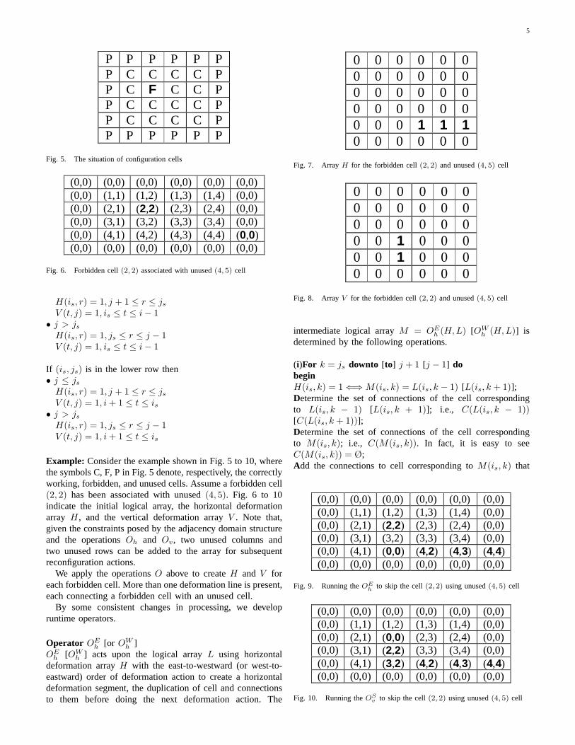
P P P P P P P C C C C P P C F C C P P C C C C P P C C C C P P P P P P P

Fig. 5. The situation of configuration cells

(0,0) (0,0) (0,0) (0,0) (0,0) (0,0) (0,0) (1,1) (1,2) (1,3) (1,4) (0,0) (0,0) (2,1) (2,2) (2,3) (2,4) (0,0) (0,0) (3,1) (3,2) (3,3) (3,4) (0,0) (0,0) (4,1) (4,2) (4,3) (4,4) (0,0) (0,0) (0,0) (0,0) (0,0) (0,0) (0,0)

Fig. 6. Forbidden cell(2, 2) associated with unused(4, 5) cell

H(is, r) = 1, j + 1 ≤ r ≤ js

V (t, j) = 1, is ≤ t ≤ i− 1• j > js

H(is, r) = 1, js ≤ r ≤ j − 1V (t, j) = 1, is ≤ t ≤ i− 1

If (is, js) is in the lower row then• j ≤ js

H(is, r) = 1, j + 1 ≤ r ≤ js

V (t, j) = 1, i + 1 ≤ t ≤ is• j > js

H(is, r) = 1, js ≤ r ≤ j − 1V (t, j) = 1, i + 1 ≤ t ≤ is

Example: Consider the example shown in Fig. 5 to 10, wherethe symbols C, F, P in Fig. 5 denote, respectively, the correctlyworking, forbidden, and unused cells. Assume a forbidden cell(2, 2) has been associated with unused(4, 5). Fig. 6 to 10indicate the initial logical array, the horizontal deformationarray H, and the vertical deformation arrayV . Note that,given the constraints posed by the adjacency domain structureand the operationsOh and Ov, two unused columns andtwo unused rows can be added to the array for subsequentreconfiguration actions.

We apply the operationsO above to createH and V foreach forbidden cell. More than one deformation line is present,each connecting a forbidden cell with an unused cell.

By some consistent changes in processing, we developruntime operators.

Operator OEh [or OW

h ]OE

h [OWh ] acts upon the logical arrayL using horizontal

deformation arrayH with the east-to-westward (or west-to-eastward) order of deformation action to create a horizontaldeformation segment, the duplication of cell and connectionsto them before doing the next deformation action. The

0 0 0 0 0 0 0 0 0 0 0 0 0 0 0 0 0 0 0 0 0 0 0 0 0 0 0 1 1 1 0 0 0 0 0 0

Fig. 7. ArrayH for the forbidden cell(2, 2) and unused(4, 5) cell

0 0 0 0 0 0 0 0 0 0 0 0 0 0 0 0 0 0 0 0 1 0 0 0 0 0 1 0 0 0 0 0 0 0 0 0

Fig. 8. ArrayV for the forbidden cell(2, 2) and unused(4, 5) cell

intermediate logical arrayM = OEh (H, L) [OW

h (H,L)] isdetermined by the following operations.

(i)For k = js downto [to] j + 1 [j − 1] dobeginH(is, k) = 1 ⇐⇒ M(is, k) = L(is, k − 1) [L(is, k + 1)];Determine the set of connections of the cell correspondingto L(is, k − 1) [L(is, k + 1)]; i.e., C(L(is, k − 1))[C(L(is, k + 1))];Determine the set of connections of the cell correspondingto M(is, k); i.e., C(M(is, k)). In fact, it is easy to seeC(M(is, k)) = Ø;Add the connections to cell corresponding toM(is, k) that

(0,0) (0,0) (0,0) (0,0) (0,0) (0,0) (0,0) (1,1) (1,2) (1,3) (1,4) (0,0) (0,0) (2,1) (2,2) (2,3) (2,4) (0,0) (0,0) (3,1) (3,2) (3,3) (3,4) (0,0) (0,0) (4,1) (0,0) (4,2) (4,3) (4,4) (0,0) (0,0) (0,0) (0,0) (0,0) (0,0)

Fig. 9. Running theOEh to skip the cell(2, 2) using unused(4, 5) cell

(0,0) (0,0) (0,0) (0,0) (0,0) (0,0) (0,0) (1,1) (1,2) (1,3) (1,4) (0,0) (0,0) (2,1) (0,0) (2,3) (2,4) (0,0) (0,0) (3,1) (2,2) (3,3) (3,4) (0,0) (0,0) (4,1) (3,2) (4,2) (4,3) (4,4) (0,0) (0,0) (0,0) (0,0) (0,0) (0,0)

Fig. 10. Running theOSv to skip the cell(2, 2) using unused(4, 5) cell

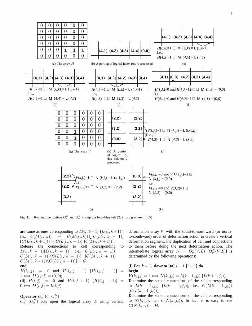
6

0 0 0 0 0 0 0 0 0 0 0 0 0 0 0 0 0 0 0 0 0 0 0 0 0 0 0 1 1 1 0 0 0 0 0 0

(a) The arrayH

(4,1) (4,2) (4,3) (4,4) (0,0)

(b) A portion of logical index row4 processed

H(is,k)=1 ⇔ M (is,k) = L (is,k-1) i.e., H(4,5)=1 ⇔ M (4,5) = L (4,4)

(4,1) (4,2) (4,3) (4,4) (4,4)

(c)

H(is,k)=1 ⇔ M (is,k) = L (is,k-1) i.e., H(4,4)=1 ⇔ M (4,4) = L (4,3)

(4,1) (4,2) (4,3) (4,3) (4,4)

(d)

H(is,k)=1 ⇔ M (is,k) = L (is,k-1) i.e., H(4,3)=1 ⇔ M (4,3) = L (4,2)

(4,1) (4,2) (4,2) (4,3) (4,4)

(e)

H(is,k)=0 and H(is,k+1)=1 ⇔ M (is,k) = (0,0) i.e., H(4,1)=0 and H(4,2)=1 ⇔ M (4,1) = (0,0)

(4,1) (0,0) (4,2) (4,3) (4,4)

(f)

0 0 0 0 0 0 0 0 0 0 0 0 0 0 0 0 0 0 0 0 1 0 0 0 0 0 1 0 0 0 0 0 0 0 0 0

(g) The arrayV

(0,0)

(3,2)

(2,2)

(h) A portion

of logical in-dex column 2processed

V(k,js)=1 ⇔ N (k,js) = L (k-1,js) i.e., V(4,2)=1 ⇔ N (4,2) = L (3,2) (3,2)

(3,2)

(2,2)

(i)

V(k,js)=1 ⇔ N (k,js) = L (k-1,js) i.e., V(3,2)=1 ⇔ N (3,2) = L (2,2)

(3,2)

(2,2)

(2,2)

(j)

V(k,js)=0 and V(k+1,js)=1 ⇔ N (k,js) = (0,0) i.e., V(2,2)=0 and V(3,2)=1 ⇔ N (2,2) = (0,0) (3,2)

(2,2)

(0,0)

(k)

Fig. 11. Running the runtimeOEh andOS

v to skip the forbidden cell(2, 2) using unused(4, 5)

are same as ones corresponding toL(is, k− 1) [L(is, k +1)];i.e., C(M(is, k)) = C(M(is, k))

⋃C(L(is, k − 1))

[C(L(is, k + 1))] = C(L(is, k − 1)) [C(L(is, k + 1))];Release the connections to cell corresponding toL(is, k − 1)[L(is, k + 1)]; i.e., C(L(is, k − 1)) =C(L(is, k − 1))\C(L(is, k − 1)) [C(L(is, k + 1)) =C(L(is, k + 1))\C(L(is, k + 1))] = Ø;endH(is, j) = 0 and H(is, j + 1) [H(is, j − 1)] =1 ⇐⇒ M(is, j) = (0, 0);(ii ) H(i, j) = 0 and H(i, j + 1) [H(i, j − 1)] =0 ⇐⇒ M(i, j) = L(i, j)

Operator OSv [or ON

v ]OS

v [ONv ] acts upon the logical arrayL using vertical

deformation arrayV with the south-to-northward (or north-to-southward) order of deformation action to create a verticaldeformation segment, the duplication of cell and connectionsto them before doing the next deformation action. Theintermediate logical arrayN = OS

v (V, L) [ONv (V, L)] is

determined by the following operations:

(i) For k = is downto [to] i + 1 [i− 1] dobeginV (k, js) = 1 ⇐⇒ N(k, js) = L(k − 1, js) [L(k + 1, js)];Determine the set of connections of the cell correspondingto L(k − 1, js) [L(k + 1, js)]; i.e., C(L(k − 1, js))[C(L(k + 1, js))];Determine the set of connections of the cell correspondingto N(k, js); i.e., C(N(k, js)). In fact, it is easy to seeC(N(k, js)) = Ø;

7

Add the connections to cell corresponding toN(k, js) thatare same as ones corresponding toL(k−1, js) [L(k +1, js)];i.e., C(N(k, js)) = C(N(k, js))

⋃C(L(k − 1, js))

[C(L(k + 1, js))] = C(L(k − 1, js)) [C(L(k + 1, js))];Release the connections to cell corresponding toL(k− 1, js)[L(k+1, js)]; i.e.,C(L(k−1, js)) = C(L(k−1, js))\C(L(k−1, js)) [C(L(k + 1, js)) = C(L(k + 1, js))\C(L(k + 1, js))]= Ø;endV (i, js) = 0 and V (i + 1, js) [V (i − 1, js)] =1 ⇐⇒ N(i, js) = (0, 0);(ii ) V (i, j) = 0 and V (i + 1, j) [V (i − 1, j)] =0 ⇐⇒ N(i, j) = L(i, j)

Example: As in Fig. 5 to 10, the tables in Fig. 11 illustratein detail the order of operations ofOE

h , OSv based on the

arraysH andV .

VI. RECONFIGURATIONRULES

Until now, we have been able to formulate thereconfiguration rules as follows:

All forbidden-free cells

Rule M.1.1. If the cell (i, j) is uninvolved then it is acorresponding target of logical index(i, j)

There exists a forbidden cell

Rule M.2.1.If the cell (i, j) is forbidden, an unused cell(is, js) on theright column andi ≤ is then create the arraysH, V afterthat applying the operatorsOE

h (H,L) andOSv (V, L).

It will be denoted by〈(i, j), (is, js), i ≤ is, j < js〉 M.2.1=⇒〈H, OE

h (H,L)〉 and 〈V, OSv (V,L)〉

Rule M.2.2.〈(i, j), (is, js), i > is, j < js〉 M.2.2=⇒ 〈H,OE

h (H, L)〉 and〈V, ON

v (V, L)〉i.e., if the cell (i, j) is forbidden, an unused cell(is, js) onthe right column andi > is then create the arraysH, V afterthat applying the operatorsOE

h (H,L) andONv (V, L).

Rule M.2.3.〈(i, j), (is, js), i ≤ is, j > js〉 M.2.3=⇒ 〈H,OW

h (H,L)〉 and〈V, OS

v (V,L)〉i.e., if the cell (i, j) is forbidden, an unused cell(is, js) onthe left column andi ≤ is then create the arraysH, V andapplying the operatorsOW

h (H, L) andOSv (V,L).

Rule M.2.4.〈(i, j), (is, js), i > is, j > js〉 M.2.4=⇒ 〈H,OW

h (H,L)〉 and〈V, ON

v (V, L)〉i.e., if the cell (i, j) is forbidden, an unused cell(is, js) onthe left column andi > is then create the arraysH, V andapplying the operatorsOW

h (H, L) andONv (V, L).

Rule M.2.5.〈(i, j), (is, js), i < is, j ≤ js〉 M.2.5=⇒ 〈V, ON

v (V, L)〉 and〈H, OE

h (H,L)〉i.e., if the cell (i, j) is forbidden, an unused cell(is, js) on

the top row andj ≤ js then create the arraysH, V andapplying the operatorsON

v (V,L) andOEh (H, L).

Rule M.2.6.〈(i, j), (is, js), i < is, j > js〉 M.2.6=⇒ 〈V, ON

v (V, L)〉 and〈H, OW

h (H, L)〉i.e., if the cell (i, j) is forbidden, an unused cell(is, js) onthe top row andj > js then create the arraysH, V andapplying the operatorsON

v (V,L) andOWh (H, L).

Rule M.2.7.〈(i, j), (is, js), i > is, j ≤ js〉 M.2.6=⇒ 〈V, OS

v (V,L)〉 and〈H, OE

h (H, L)〉i.e., if the cell (i, j) is forbidden, an unused cell(is, js) onthe lower row andj ≤ js then create the arraysH, V andapplying the operatorsOS

v (V, L) andOEh (H,L).

Rule M.2.8.〈(i, j), (is, js), i > is, j > js〉 M.2.8=⇒ 〈V, OS

v (V,L)〉 and〈H, OW

h (H, L)〉i.e., if the cell (i, j) is forbidden, an unused cell(is, js) onthe lower row andj > js then create the arraysH, V andapplying the operatorsOS

v (V, L) andOWh (H,L).

VII. R ECONFIGURATIONCONSEQUENCE AS AN

INVARIANT

We will show that the reconfiguration consequence is justan invariant in this section.

1) Reconfiguration consequence:A logical array X is areconfiguration consequence ofL (written L |⊂ X) iff thepartial correction ofL is also preserved inX.

2) Provability: A logical array X is provable fromL(written L ` X) iff X is a result ofL by the reconfigurationrules.

Before considering the soundness of the reconfigurationrules we prove the following lemmas.

Lemma 7.1:Rule M.1.1 creates a partially correct logicalarray

Proof: This follows from the definition 4.6Lemma 7.2:Rule M.2.1 creates a partially correct logical

arrayProof: A partial correction must satisfy two constraints

that every logical indexL(i, j) 6= (0, 0) is not duplicated andthat the logical indexL(i, j) = (0, 0) does not appear inXdue to the locality of the cell adjacency domain (as in thedefinition of partially correct logical array above). We willprove that any logical array created by ruleM.2.1 satisfy theseabove two constraints.

Firstly, we prove every logical indexL(i, j) 6= (0, 0) isnot duplicated by ruleM.2.1. Let the logical indexesX(i′, j′)andX(i”, j”) be not(0, 0) andL be a partially correct logicalarray. Suppose that(i, j) be a cell with initial logical indexesL(i, j) = X(i′, j′) = X(i”, j”). This cell is unique from thedefinition of L as a partially correct logical array. For theeastward horizontal operatorOE

h (H,L) of rule M.2.1, it isi = i′ = i”. By operation (i) of OE

h (H, L), j′ = j” = j − 1or by operation (ii ) of OE

h (H, L), j′ = j” = j, if j′ 6= j”thenj′ = j andj” = j + 1 or vice versa. By operation (i), ifj” = j+1 = j′+1 thenH(i′, j′+1) = 1. By operation (ii ), ifj′ = j thenH(i′, j′) = 0. By operation (i), if H(i′, j′+1) = 1

8

and H(i′, j′) = 0 then X(i′, j′) = (0, 0). This contradictsthe hypothesis of logical indexesX(i′, j′) 6= (0, 0). Hence,every logical indexL(i, j) 6= (0, 0) is not duplicated underthe operatorOE

h (H, L). In the same way, every logical indexL(i, j) 6= (0, 0) is not also duplicated under the southwardvertical operatorOS

v (V, L).Secondly, we prove that the logical indexesL(k, h) = (0, 0)

do not appear inX. Suppose thatL is a partially correct logicalarray andL(i, j) 6= (0, 0) for each cell for whichH(i, j) = 1and H(i, j + 1) = 0. Due to H(i, j) = 1, then X(i, j) =L(i, j−1) by operation (i) of OE

h (H, L). X(i, j+1) = L(i, j)iff H(i, j+1) = 1 by operation (i) as well. This contradicts theabove hypothesis; hence the logical indexes that do not appearin X are zero inL under the operatorOE

h (H,L). Similarly,under the operatorOS

v (V,L), the logical indexesL(k, h) =(0, 0) do not also appear inX; see an illustration in Fig. 12.X, created fromL by rule M.2.1, is then partially correct.

H�(i,j)=1 H�(i,j+1)=0 H�(i,j+2)=1

�(i,j)≠(0,0)

�(i,j+1)=(0,0)

H�(i,j)=1 H�(i,j+1)=1

�(i,j)= �(i,j-1)

�(i,j+1)= �(i,j)

Fig. 12. Logical indexL(i, j +1) = (0, 0) does not appear inX under theoperatorOE

h (H, L)

Lemma 7.3:Every rule of M.2.2, M.2.3, M.2.4, M.2.5,M.2.6, M.2.7 and M.2.8 creates a partially correct logicalarray

Proof: The proof steps are similar to those for lemma 7.2.

Theorem 7.4 (Soundness):If L ` X thenL |⊂ XProof: This is a consequence of the lemmas 7.1, 7.2,

and 7.3 above.

VIII. R ECONFIGURATION AS ACOMPLETE MATCHING

PROBLEM

Reconfiguration is now defined simply as the search for amapping of logical indexes onto configuration cells, given apredetermined adjacency domain of cells. It will be seen thatsuch a problem can be described by means of acompletematchingproblem [3].

Let X = {x1, x2, . . . , xm} and Y = {y1, y2, . . . , yn} betwo finite sets withm logical indexes andn forbidden-freecells, respectively. It is obvious thatX

⋂Y = Ø. Let 4 be a

collection of pairse = {x, y} wherex ∈ X andy ∈ Y .The tripleG = (X,4, Y ) is called abipartite graph. The

elements ofX⋃

Y are called the vertices ofG, andX,Y iscalled a bipartition (partition into two parts) of the verticesof G. The pairse = {x, y} in 4 are called the edges ofG,

x1 x2 … xi xi+1 xi+2 … x2i … … … … xki+1 xki+2 … x(k+1)i

(a)

y1 y2 y3 … yj yj+1 yj+2 yj+3 … y2j y2j+1 y2j+2 y2j+3 … y3j … … … … … ypj+1 ypj+2 ypj+3 … y(p+1)j

(b)

y1 y2 y3 … y(p+1)j x1 x x x … x x2 x x x … x ... … … … … … x(k+1)i x x x … x

(c)

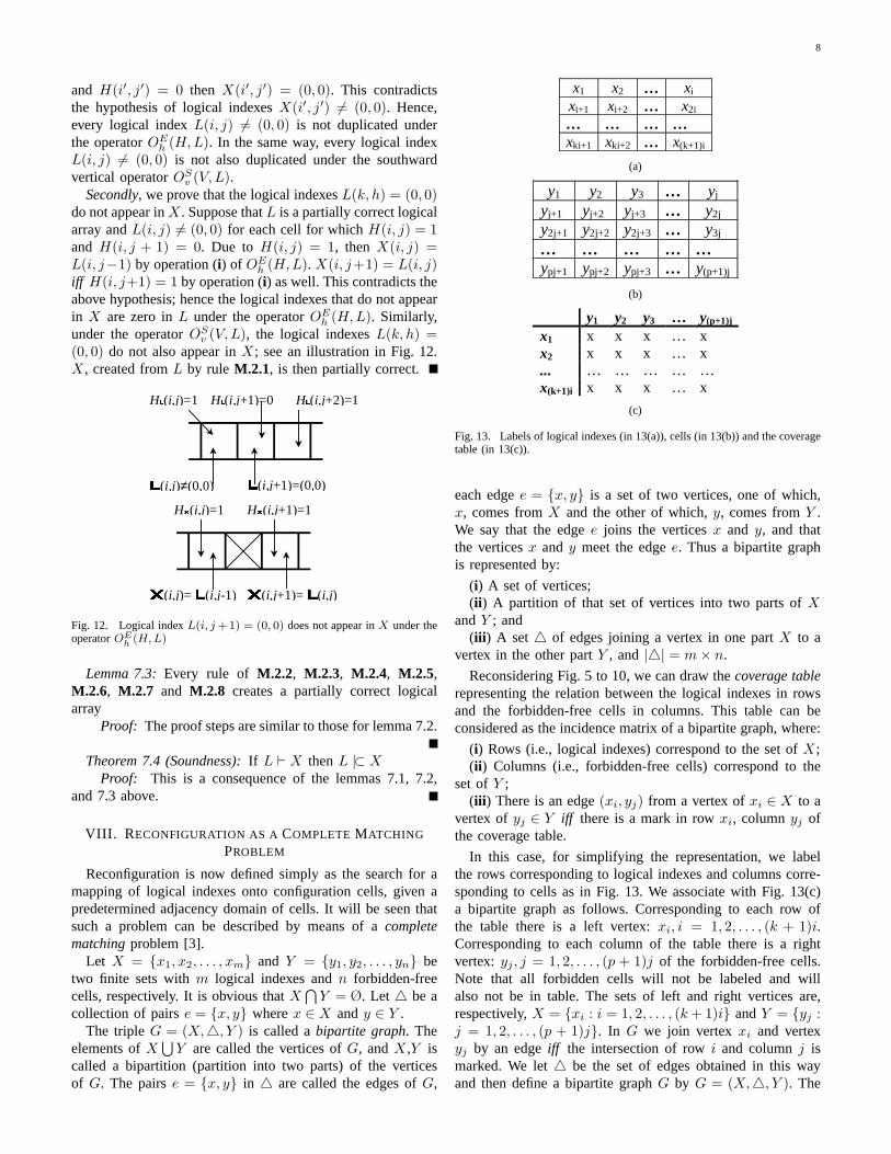
Fig. 13. Labels of logical indexes (in 13(a)), cells (in 13(b)) and the coveragetable (in 13(c)).

each edgee = {x, y} is a set of two vertices, one of which,x, comes fromX and the other of which,y, comes fromY .We say that the edgee joins the verticesx and y, and thatthe verticesx and y meet the edgee. Thus a bipartite graphis represented by:

(i) A set of vertices;(ii ) A partition of that set of vertices into two parts ofX

andY ; and(iii ) A set4 of edges joining a vertex in one partX to a

vertex in the other partY , and |4| = m× n.

Reconsidering Fig. 5 to 10, we can draw thecoverage tablerepresenting the relation between the logical indexes in rowsand the forbidden-free cells in columns. This table can beconsidered as the incidence matrix of a bipartite graph, where:

(i) Rows (i.e., logical indexes) correspond to the set ofX;(ii ) Columns (i.e., forbidden-free cells) correspond to the

set ofY ;(iii ) There is an edge(xi, yj) from a vertex ofxi ∈ X to a

vertex ofyj ∈ Y iff there is a mark in rowxi, columnyj ofthe coverage table.

In this case, for simplifying the representation, we labelthe rows corresponding to logical indexes and columns corre-sponding to cells as in Fig. 13. We associate with Fig. 13(c)a bipartite graph as follows. Corresponding to each row ofthe table there is a left vertex:xi, i = 1, 2, . . . , (k + 1)i.Corresponding to each column of the table there is a rightvertex: yj , j = 1, 2, . . . , (p + 1)j of the forbidden-free cells.Note that all forbidden cells will not be labeled and willalso not be in table. The sets of left and right vertices are,respectively,X = {xi : i = 1, 2, . . . , (k + 1)i} andY = {yj :j = 1, 2, . . . , (p + 1)j}. In G we join vertexxi and vertexyj by an edgeiff the intersection of rowi and columnj ismarked. We let4 be the set of edges obtained in this wayand then define a bipartite graphG by G = (X,4, Y ). The

9

set4 of edges ofG is in 1-1 correspondence with the marksof the table.

IX. A H EURISTIC FORRECONFIGURATION

Prior to describing the algorithmic approach using ourheuristic for matching, some definitions are presented.

Definition 9.1: MatchingA matchM is a subset of edges ofG(M ⊂ 4) such that notwo edges have an end-point in common.

Definition 9.2: Maximum matchingA match is called maximum if no other match contains moreedges.

To solve the reconfiguration problem, our heuristic is spec-ified with respect to three issues for problem solving [15]:representation of search space, objectiveandstarting point.

A. Representation of search space

We will encode alternative candidate solutions for manipu-lation. In other words, the representation of a potential matchand its corresponding interpretation implies thesearch spaceand itssize. For this purpose, thecoverage tableis consideredas a representation of search space of potential matches.

Let S be the search space of potential maximum matches.Each elementx of S is a maximum match and must satisfythe following two conditions:

(i) Each logical index must be associated with a cell, sothere isonemark in each row of coverage table.

(ii ) No cell can be associated with more than one logicalindex, so there isat most onemark in each column.

The size ofS is the number of different maximum matchesin S, written as |S|, and determined as follows. Letn andm be the number of columns and rows of coverage tablerespectively, wheren ≥ m. It is obvious that the valueof |S| is just the largest number of maximum matches. Inother words, it is calculated by the following expression:|S| = n × (n − 1) × (n − 2) × . . . × (n − m), wheren isthe number of possible selections of a mark on the first row,(n− 1) corresponds to the number of possible selections of amark on the second row,. . ., and(n−m) corresponds to thenumber of possible selections of a mark on themth row.

B. Objective

Once we defined the search space, we have to decide forwhat it is that we are searching. What is the objective of ourproblem? This should be a mathematical statement of the taskto be achieved. Here, the objective is typically any maximummatch that satisfies the total correction of a logical array. Inmathematical terms, letSsol be a set of the solutions (i.e.,the maximum matches satisfying the total correction of thelogical array). Hence,Ssol ⊂ S and our objective is to findany maximum matchx ∈ Ssol ⊂ S.

To build Ssol we separate it into two cases, existingforbidden-free and forbidden cells. If all forbidden-free cellsthenSsol = {(xi, yi), i = 1, 2, . . . , m} as a result of applyingrule M.1.1 and in this casex is easy to determine:x ={(xi, yi), i = 1, 2, . . . , m} ∈ Ssol. If there are some forbidden

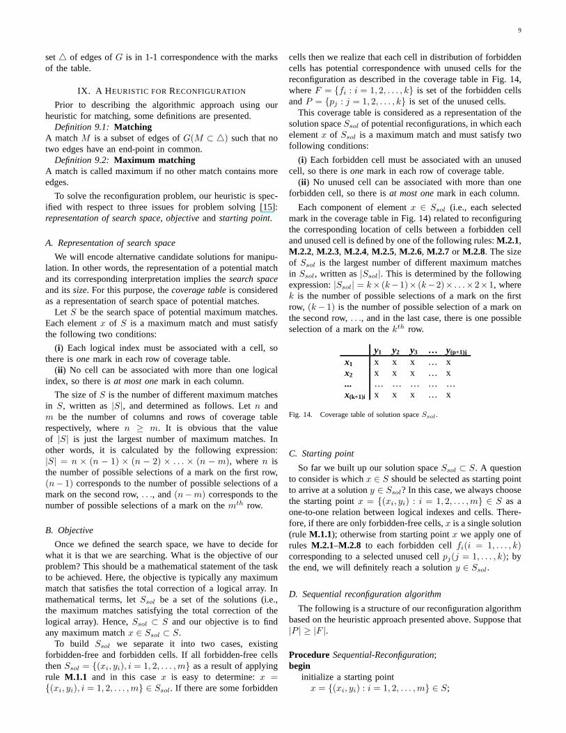
cells then we realize that each cell in distribution of forbiddencells has potential correspondence with unused cells for thereconfiguration as described in the coverage table in Fig. 14,whereF = {fi : i = 1, 2, . . . , k} is set of the forbidden cellsandP = {pj : j = 1, 2, . . . , k} is set of the unused cells.

This coverage table is considered as a representation of thesolution spaceSsol of potential reconfigurations, in which eachelementx of Ssol is a maximum match and must satisfy twofollowing conditions:

(i) Each forbidden cell must be associated with an unusedcell, so there isonemark in each row of coverage table.

(ii ) No unused cell can be associated with more than oneforbidden cell, so there isat most onemark in each column.

Each component of elementx ∈ Ssol (i.e., each selectedmark in the coverage table in Fig. 14) related to reconfiguringthe corresponding location of cells between a forbidden celland unused cell is defined by one of the following rules:M.2.1,M.2.2, M.2.3, M.2.4, M.2.5, M.2.6, M.2.7 or M.2.8. The sizeof Ssol is the largest number of different maximum matchesin Ssol, written as|Ssol|. This is determined by the followingexpression:|Ssol| = k× (k−1)× (k−2)× . . .×2×1, wherek is the number of possible selections of a mark on the firstrow, (k− 1) is the number of possible selection of a mark onthe second row,. . ., and in the last case, there is one possibleselection of a mark on thekth row.

y1 y2 y3 … y(p+1)j x1 x x x … x x2 x x x … x ... … … … … … x(k+1)i x x x … x

Fig. 14. Coverage table of solution spaceSsol.

C. Starting point

So far we built up our solution spaceSsol ⊂ S. A questionto consider is whichx ∈ S should be selected as starting pointto arrive at a solutiony ∈ Ssol? In this case, we always choosethe starting pointx = {(xi, yi) : i = 1, 2, . . . ,m} ∈ S as aone-to-one relation between logical indexes and cells. There-fore, if there are only forbidden-free cells,x is a single solution(rule M.1.1); otherwise from starting pointx we apply one ofrules M.2.1–M.2.8 to each forbidden cellfi(i = 1, . . . , k)corresponding to a selected unused cellpj(j = 1, . . . , k); bythe end, we will definitely reach a solutiony ∈ Ssol.

D. Sequential reconfiguration algorithm

The following is a structure of our reconfiguration algorithmbased on the heuristic approach presented above. Suppose that|P | ≥ |F |.

Procedure Sequential-Reconfiguration;begin

initialize a starting pointx = {(xi, yi) : i = 1, 2, . . . , m} ∈ S;

10

if F = Ø then run the ruleM.1.1;while F 6= Ø dobegin

selectf ∈ F ;selectp ∈ P ;run one of rulesM.2.1-M.2.8 according tothe relation of location betweenf andp;F = F\{f};P = P\{p};

endend

Analysis and computational complexity of sequential re-configuration algorithm:The computational complexity implies the computational time,which is just the time needed for computing the deformationoperations in the selected rulesM.2.1–M.2.8 in all iterationsof the while loop. In other words, the computational timemeasured by the number of values1 in the arraysH andV of the deformation operations because each value1 in thearraysH and V determines a horizontal and vertical moverespectively.

Let 1(H) and1(V ) be the functions determining the numberof values1 in the arrayH andV ; then they are1(H) =

∑hij ,

with ∀hij ∈ H and 1(V ) =∑

vij , with ∀vij ∈ V . Ineach iteration of thewhile loop, the number of horizontaland vertical moves are1(H) + 1(V ) =

∑hij +

∑vij , with

∀hij ∈ H and∀vij ∈ V , and the total number of moves forall iterations are

∑|F |(1(H) + 1(V )), where|F | is equal to

the number of elements of the setF . Therefore its complexityis O(|F |n), wheren = max(1(H) + 1(V )) over the setF . Indetermining this computational complexity, we realize that toreduce the number of moves1(H) + 1(V ), we must suitablyselect the pair of(f, p) so that ∀f, ∃p: minimal (1(H) +1(V )); i.e., local minimum(1(H) + 1(V )) or min(1(H) +1(V )) for short and the total number of moves of all iterationsare

∑|F |min(1(H) + 1(V )). This is just the reduced number

of computations of the followingReconfiguration*algorithm,modified from the earlierReconfigurationalgorithm.

Procedure Sequential-Reconfiguration*;begin

initialize a starting pointx = {(xi, yi) : i = 1, 2, . . . , m} ∈ S;

if F = Ø then run the ruleM.1.1;while F 6= Ø dobegin

selectf ∈ F ;selectp ∈ P so that∀f,∃p: min(1(H) + 1(V ));run one of rulesM.2.1-M.2.8 according tothe relation of location betweenf andp;F = F\{f};P = P\{p};

endend

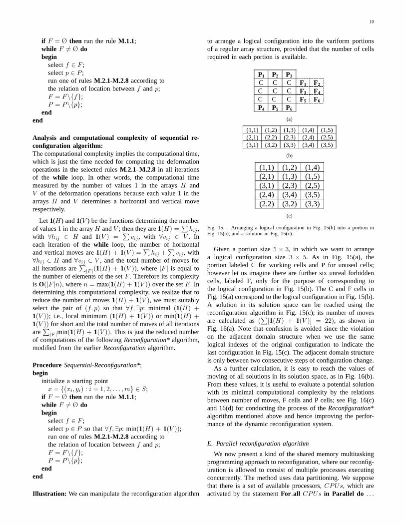
Illustration: We can manipulate the reconfiguration algorithm

to arrange a logical configuration into the variform portionsof a regular array structure, provided that the number of cellsrequired in each portion is available.

P1 P2 P3 C C C F1 F2 C C C F3 F4 C C C F5 F6 P4 P5 P6 (a)

(1,1) (1,2) (1,3) (1,4) (1,5) (2,1) (2,2) (2,3) (2,4) (2,5) (3,1) (3,2) (3,3) (3,4) (3,5) (b)

(1,1) (1,2) (1,4) (2,1) (1,3) (1,5) (3,1) (2,3) (2,5) (2,4) (3,4) (3,5) (2,2) (3,2) (3,3)

(c)

Fig. 15. Arranging a logical configuration in Fig. 15(b) into a portion inFig. 15(a), and a solution in Fig. 15(c).

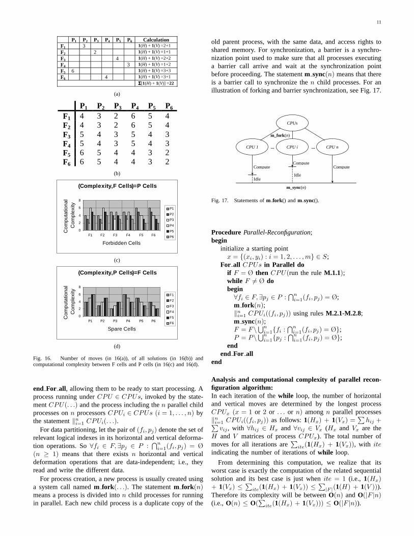
Given a portion size5 × 3, in which we want to arrangea logical configuration size3 × 5. As in Fig. 15(a), theportion labeled C for working cells and P for unused cells;however let us imagine there are further six unreal forbiddencells, labeled F, only for the purpose of corresponding tothe logical configuration in Fig. 15(b). The C and F cells inFig. 15(a) correspond to the logical configuration in Fig. 15(b).A solution in its solution space can be reached using thereconfiguration algorithm in Fig. 15(c); its number of movesare calculated as(

∑[1(H) + 1(V )] = 22), as shown in

Fig. 16(a). Note that confusion is avoided since the violationon the adjacent domain structure when we use the samelogical indexes of the original configuration to indicate thelast configuration in Fig. 15(c). The adjacent domain structureis only between two consecutive steps of configuration change.

As a further calculation, it is easy to reach the values ofmoving of all solutions in its solution space, as in Fig. 16(b).From these values, it is useful to evaluate a potential solutionwith its minimal computational complexity by the relationsbetween number of moves, F cells and P cells; see Fig. 16(c)and 16(d) for conducting the process of theReconfiguration*algorithm mentioned above and hence improving the perfor-mance of the dynamic reconfiguration system.

E. Parallel reconfiguration algorithm

We now present a kind of the shared memory multitaskingprogramming approach to reconfiguration, where our reconfig-uration is allowed to consist of multiple processes executingconcurrently. The method uses data partitioning. We supposethat there is a set of available processors,CPUs, which areactivated by the statementFor all CPUs in Parallel do . . .

11

P1 P2 P3 P4 P5 P6 Calculation F1 3 1(H) + 1(V) =2+1

F2 2 1(H) + 1(V) =1+1

F3 4 1(H) + 1(V) =2+2

F4 3 1(H) + 1(V) =1+2

F5 6 1(H) + 1(V) =3+3

F6 4 1(H) + 1(V) =3+1

ΣΣΣΣ[1(H) + 1(V)] =22

(a)

P1 P2 P3 P4 P5 P6 F1 4 3 2 6 5 4 F2 4 3 2 6 5 4 F3 5 4 3 5 4 3 F4 5 4 3 5 4 3 F5 6 5 4 4 3 2 F6 6 5 4 4 3 2

(b)

(Complexity,F Cells)=P Cells

0

2

4

6

8

F1 F2 F3 F4 F5 F6

Forbidden Cells

Com

puta

tiona

l C

ompl

exity

P1

P2

P3

P4

P5

P6

(c)

(Complexity,P Cells)=F Cells

0

2

4

6

8

P1 P2 P3 P4 P5 P6

Spare Cells

Com

puta

tiona

l C

ompl

exity

F1

F2

F3

F4

F5

F6

(d)

Fig. 16. Number of moves (in 16(a)), of all solutions (in 16(b)) andcomputational complexity between F cells and P cells (in 16(c) and 16(d).

end For all, allowing them to be ready to start processing. Aprocess running underCPU ∈ CPUs, invoked by the state-mentCPU(. . .) and the process including then parallel childprocesses onn processorsCPUi ∈ CPUs (i = 1, . . . , n) bythe statement‖n

i=1 CPUi(. . .).For data partitioning, let the pair of(fi, pj) denote the set of

relevant logical indexes in its horizontal and vertical deforma-tion operations. So∀fi ∈ F,∃pj ∈ P :

⋂ni=1(fi, pj) = Ø

(n ≥ 1) means that there existsn horizontal and verticaldeformation operations that are data-independent; i.e., theyread and write the different data.

For process creation, a new process is usually created usinga system call namedm fork (. . .). The statementm fork (n)means a process is divided inton child processes for runningin parallel. Each new child process is a duplicate copy of the

old parent process, with the same data, and access rights toshared memory. For synchronization, a barrier is a synchro-nization point used to make sure that all processes executinga barrier call arrive and wait at the synchronization pointbefore proceeding. The statementm sync(n) means that thereis a barrier call to synchronize then child processes. For anillustration of forking and barrier synchronization, see Fig. 17.

... ...

Idle Idle

Compute Compute

Compute

m_fork(n)

m_sync(n)

CPUs

CPU n CPU i CPU 1

Fig. 17. Statements ofm fork () andm sync().

Procedure Parallel-Reconfiguration;begin

initialize a starting pointx = {(xi, yi) : i = 1, 2, . . . , m} ∈ S;

For all CPUs in Parallel doif F = Ø then CPU(run the ruleM.1.1);while F 6= Ø dobegin∀fi ∈ F, ∃pj ∈ P :

⋂ni=1(fi, pj) = Ø;

m fork (n);‖n

i=1 CPUi((fi, pj)) using rulesM.2.1-M.2.8;m sync(n);F = F\⋃n

i=1{fi :⋂n

i=1(fi, pj) = Ø};P = P\⋃n

i=1{pj :⋂n

i=1(fi, pj) = Ø};end

end For allend

Analysis and computational complexity of parallel recon-figuration algorithm:In each iteration of thewhile loop, the number of horizontaland vertical moves are determined by the longest processCPUx (x = 1 or 2 or . . . or n) amongn parallel processes‖n

i=1 CPUi((fi, pj)) as follows:1(Hx) + 1(Vx) =∑

hij +∑vij , with ∀hij ∈ Hx and ∀vij ∈ Vx (Hx and Vx are the

H and V matrices of processCPUx). The total number ofmoves for all iterations are

∑ite(1(Hx) + 1(Vx)), with ite

indicating the number of iterations ofwhile loop.

From determining this computation, we realize that itsworst case is exactly the computation of the related sequentialsolution and its best case is just whenite = 1 (i.e., 1(Hx)+ 1(Vx) ≤ ∑

ite(1(Hx) + 1(Vx)) ≤ ∑|F |(1(H) + 1(V ))).

Therefore its complexity will be betweenO(n) andO(|F |n)(i.e., O(n) ≤ O(

∑ite(1(Hx) + 1(Vx))) ≤ O(|F |n)).

12

Illustration: Referring back to the illustration in Fig. 15(a)and 15(b) above, this time we consider processing by theparallel reconfiguration algorithm. We immediately realize thatthe connection betweenfi and pj can be partitioned intosome pairs of(fi, pj) to reach a solution under the constraint∀fi ∈ F,∃pj ∈ P.

⋂ni=1(fi, pj) = Ø as follows:

(f1, p3)⋂

(f3, p2)⋂

(f5, p1) = Ø(f2, p4)

⋂(f4, p5)

⋂(f6, p6) = Ø

and its number of moves are calculated as(∑

2[1(Hx) +1(Vx)] = 12), as shown in Fig. 18(a).

As a comparison, if this solution is reached by the sequentialalgorithm its computation will be(

∑[1(H) + 1(V )] = 24),

as in Fig. 18(b).Obviously, this parallel approach improves the performance

better than the sequential one with reduced computation time.

P1 P2 P3 P4 P5 P6 F1 F2 6 F3 F4 F5 6 F6

(a)

P1 P2 P3 P4 P5 P6 F1 2 F2 6 F3 4 F4 4 F5 6 F6 2

(b)

Fig. 18. Number of moves of parallel solution (in 18(a)) and serial solution(in 18(b)).

X. CONCLUSION

For the continuous evolution of dynamically reconfigurablecomputing in embedded systems, we have considered how toreconfigure an embedding of a graph into a regular array usinggraph transformations. These transformations are bounded byadjacency constraints, which mean that connected nodes of agraph are still embedded adjacently after the execution of agraph transformation rule. An important contribution is thatusing the suggested approach, continuous evolution of theapplications can be partially carried out at runtime withoutstopping the operation of the whole system. The continuityof this reorganization mechanism guarantees that invariants ofthe design are respected, dependencies can be detected andthe impact of planned changes can be determined.

Dynamic reconfiguration is likely to become increasinglyimportant in embedded systems to allow increased flexibility.

However, the added complexity can create additional oppor-tunities for errors in such systems. Particularly in safety-critical or security-critical applications, it will be importantto use formal techniques to avoid the introduction of errors.In such cases, it is hoped that a rigorous approach such as thatpresented in this paper will be applied.

REFERENCES

[1] G. Allwein and J. Barwise,Logical Reasoning with Diagrams, Oxford,England: Oxford University Press, 1996.

[2] J. P. Bowen and M. G. Hinchey, Formal methods, in A. B. Tucker, Jr.(ed.), Computer Science Handbook, 2nd edition, Section XI, SoftwareEngineering, Chapter 106, pp. 106-1–106-25, Chapman & Hall / CRC,ACM, 2004.

[3] R. A. Brualdi, Introductory Combinatorics, Upper Saddle River, NJ:Prentice Hall, 1999.

[4] K. Compton, S. Hauck, Reconfigurable computing: a survey of systemsand software.ACM Computing Surveys, June 2002 (Vol. 34, No. 2), pp.171–210.

[5] F. Distance, M. G. Sami and R. Stefanelli,Fault-tolerance and Recon-figurability Issues in Massively Parallel Architectures, IEEE, 1995, pp.340–349.

[6] M. Gericota, G. Alves, M. Silva, and J. Ferreira, Runtime managementof logic resources on reconfigurable systems,Design, Automation andTest In Europe Conference (DATE’03), Munich, Germany, 3–7 March2003, pp. 974–979.

[7] B. Graaf, M. Lormans and H. Toetenel, Embedded software engineering:The state of the practice,IEEE Software, November/December 2003(Vol. 20, No. 6), pp. 61–69.

[8] Z. Gu, S. Kodase, S. Wang and K. G. Shin, A model-based approachto system-level dependency and real-time analysis of embedded soft-ware,9th IEEE Real-Time and Embedded Technology and ApplicationsSymposium, Toronto, Canada, 27–30 May 2003, pp. 78–87.

[9] S. Guo and W. Luk. An integrated system for developing regular arraydesigns,Journal of Systems Architecture, Vol. 47 (2001), pp. 315–337.

[10] M. G. Hinchey and J. P. Bowen (eds.),Industrial-Strength FormalMethods in Practice, London: Springer-Verlag, FACIT series, 1999.

[11] E. Horta and J. W. Lockwood,PARBIT: A Tool to Transform Bitfiles toImplement Partial Reconfiguration of Field Programmable Gate Arrays(FPGAs), Washington University, Department of Computer Science,Technical Report WUCS-01-13, July 2001.

[12] M. Jamnik, Mathematical Reasoning with Diagrams: From Intuitionto Automation, Stanford University: CSLI Press & Chicago UniversityPress, 2002.

[13] S. Kodase, S. Wang, K. G. Shin, Transforming structural model toruntime model of embedded software with real-time constraints,De-sign, Automation and Test In Europe Conference (DATE’03), Munich,Germany, 3–7 March 2003, pp. 170–175.

[14] J. Kuester-Filipe, I. Poernomo, R. Reussner and S. Shukla (eds.), FormalFoundations of Embedded Software and Component-based Software Ar-chitectures (FESCA),Electronic Notes in Theoretical Computer Science,13 December 2004 (Vol. 108).

[15] Z. Michalewicz and D. B. Fogel,How to Solve it: Modern Heuristics,Berlin: Springer, 2000.

[16] P. C. Vinh and J. P. Bowen, Formalising Configuration RelocationBehaviours for Reconfigurable Computing,Proceedings of Forum onspecification & Design Languages (FDL’02), Marseille, France, 24-27September 2002 (CD-ROM).

[17] P. C. Vinh and J. P. Bowen, An algorithmic approach by heuristicsto dynamical reconfiguration of logic resources on reconfigurable FP-GAs, Proceedings of 12th ACM International Symposium on Field-Programmable Gate Arrays (FPGA 2004), Monterey, California, USA,22–24 February 2004, p. 254.