REAL OPTIONS AND AMERICAN DERIVATIVES: THE DOUBLE

CONTINUATION REGION

Anna Battauz�

Department of Finance,

and IGIER,

Bocconi University,

Milan, Italy

Marzia De Donno

Department of Decision Sciences,

Bocconi University,

Milan, Italy

Alessandro Sbuelz

Department of Mathematics, Quantitative Finance, and Econometrics,

Catholic University of Milan,

Milan, Italy

July 2011

Abstract

Relevant capital investment options and American derivatives embedded into popular secured loans can

be reduced to American option problems with an endogenous negative �interest rate�. We show that such

problems can entail a non-standard double continuation region: option exercise is optimally postponed

not only when the option is insu¢ ciently in the money but also when it is excessively in the money. We

fully characterize the existence, the monotonicity, the continuity, the limits and the asymptotic behavior

at maturity of the double free boundary that separates the exercise region from the double continuation

region. Our results apply to real options whose project values enjoy robust growth rates while investment

costs also markedly escalate. The gold loan is an in-vogue contract of collateralized borrowing whose optimal

redeeming strategy constitutes another interesting application of our results.

JEL Code: G12, G13.

�Corresponding author. E-mail: anna.battauz@unibocconi.it.

1

1 Introduction

A number of important decision-making problems in �nance can be reformulated as American option prob-

lems with an endogenous negative interest rate. Two chief examples are the prepayment option in collat-

eralized borrowing like the recently popular gold loans1 and certain relevant capital investment options.

An endogenous negative interest rate for the American derivatives embedded into loans collateralized by

tradable assets appears whenever the loan rate is above the riskfree rate. An endogenous negative interest

rate in real options appears whenever the risk-adjusted average growth rate of the project value is above

the rate used by the �rm to discount it.

We show that such decision-making problems can imply a non-standard double continuation region:

exercise is optimally postponed not only when the option is not enough in the money (the standard part of

the continuation region) but also when the option is too deep in the money (the non-standard part of the

continuation region). For �nite-maturity and perpetual American puts and calls with a negative interest

rate in a di¤usive setting, we contribute by providing a detailed analysis of the conditions that enable the

double continuation region and a comprehensive characterization of the double free boundary entailed by

such a continuation region.

Our results add to the vast literature on American options under di¤usive uncertainty, see for instance

Detemple (2006) and the references therein. We conduct an in-depth study of the existence, the monotonic-

ity, the continuity, the limits and the asymptotic behavior at maturity of both the upper and the lower free

boundary. We start from the American put problem and prove the conditions for the existence of a double

continuation region in the case of a negative interest rate via convexity, monotonicity and value-dominance

arguments (see Lamberton and Lapeyre 1996 for the standard case of a non-negative interest rate). We use

the variational inequality approach to prove the continuity of the double free boundary (see Jaillet, Lam-

berton and Lapeyre 1990 and Lamberton 1998 for the standard case). We then carefully characterize the

double free boundary near to maturity (see Evans, Kuske and Keller 2002 and Lamberton and Villenevue

2003 for the standard case). Finally, we translate the results obtained for the American put problem into

double-free-boundary statements for the American call problem via the American put-call symmetry (e.g.

Carr and Chesney 1996 and Detemple 2001).

An interesting application to gold loans complements our theoretical analysis. A gold loan is a contract

1Gold loans are familiar among Indian �nancial intermediaries. Muthoot Finance is one of the largest gold loan companies

in India. J.P. Morgan Chase started accepting gold as loan collateral from institutional players since February 2011, amid a

climate of soaring gold prices.

2

of collateralized borrowing. A mass unit (one troy ounce, say) of gold is the collateral, which the borrower

has the right to redeem at any time before or on the loan maturity. We show that, since gold is a tradable

investment asset with storage and insurance costs and without payouts, a double continuation region can

ensue: the exercise of a deep in-the-money redemption option may be optimally postponed by the borrower.

This brings a novel contribution to the existing literature on the optimal redeeming strategy of tradable

securities used as loan collateral: Xia and Zhou (2007) focus on perpetual stock loans; Ekström andWanntorp

(2008) deal with margin call stock loans; Zhang and Zhou (2009) look into stock loans in the presence of

regime switching; Liu and Xu (2010) study capped stock loans; Dai and Xu (2011) examine the impact of

the dividend-distribution criterion on the stock loan.

By investigating the general American option problem with a negative interest rate, our work thoroughly

extends the speci�c perpetual-real-option analysis developed in Battauz, De Donno and Sbuelz (2011). We

examine (possibly �nite-maturity) capital investment options akin to, for instance, the option of entering

the lucrative business of nuclear energy. Projects may have values with conspicuous growth rates even after

risk adjustment (say rates above the discount rate used by the �rm), but the overall cost of entering them is

likely to increase even more conspicuously in the future (uranium is a scarce resource and demand for safety

is de�nitely increasing). Such a hierarchy in the risk-adjusted growth/discount rates for the real option is

conducive to the non-standard optimal continuation policy.

The rest of the paper is organized as follows. Sections 2 and 3 deal with the double continuation region for

American puts and calls, respectively. Section 4 discusses the double continuation region for the redemption

option embedded in a gold loan and for some signi�cant real options. Section 5 concludes and an Appendix

conveniently remaps the specialized results of Battauz, De Donno and Sbuelz (2011) to the general milieu

of this paper.

2 The American put

We consider an American put option written on the log-normal asset X, whose drift under the valuation

measure is positive and denoted with �. We denote the volatility with �, the strike with K, and discount

rate with �. Our aim is to compute the value of the option at time t, given by

ess supt���T

Ehe��(��t) (K �X(�))+

���Fti = v(t;X(t))where

v(t; x) = sup0���T�t

E

"e���

�K � x � exp

���� �

2

2

��+ � B(�)

��+#(2.1)

3

where B is a standard Brownian motion under the valuation measure. In this section, as well as in the next

one, expectations and distributions of stochastic processes refer all to the valuation measure. For this reason

we simplify the notation, omitting the dependence on probability in the expectations, as in both formulae

above. If we denote by v1(x) the value of the perpetual American put option, i.e.

v1(x) = sup0��

E

"e���

�K � x � exp

���� �

2

2

��+ � B(�)

��+#;

then v1 dominates v; i.e.

v(t; x) � v1(x) for any t 2 [0;T ] and x � 0:

We recall some important properties of the function v in (2:1); usually stated for non-negative �; but true

regardless of the sign of � (see for instance Lamberton and Lapeyre, 1996, and Broadie and Detemple, 1997).

The value function v in (2:1) is convex and decreasing with respect to x; and for any x � 0; the function

v(t; x) is decreasing with respect to t: Summing up, we have that

(K � x)+ � v(t; x) � v(t; 0) for all t 2 [0;T ] and x � 0: (2.2)

These properties determine the shape of the free boundary interacting with the sign of �: More precisely,

if the initial value of the underlying asset X is 0; then X(t) = 0 � exp���� �2

2

�t+ � B(t)

�= 0 for any t:

Hence, for any t < T; if � � 0;

v(t; 0) = sup0���T�t

E�e��� (K � 0)+

�= sup0���T�t

e��� �K = e���0 �K = K;

whereas, if � < 0;

v(t; 0) = sup0���T�t

E�e��� (K � 0)+

�= sup0���T�t

e��� �K = e���(T�t) �K > K:

As it is well known, when � � 0 the value of the American option for x = 0 coincides with the immediate

exercise payo¤: v(t; 0) = K = (K � 0)+ : Hence in the case of nonnegative interest rates, if (K�x)+ = v(t; x)

for some x = x0 > 0; then the same equality is satis�ed (K � x)+ = v(t; x) for any x � x0 by convexity and

(2:2) (see for instance Lamberton and Lapeyre (1996)). Therefore, there exists a time t critical price

x�(t) = sup fx � 0 : v(t; x) = K � xg

such that early exercise is optimal at time t for x � x�(t); whereas for x > x�(t) it is optimal to continue.

Figure 1 portraits this analysis in the graph on the left (the dashed line represents the case where there is

4

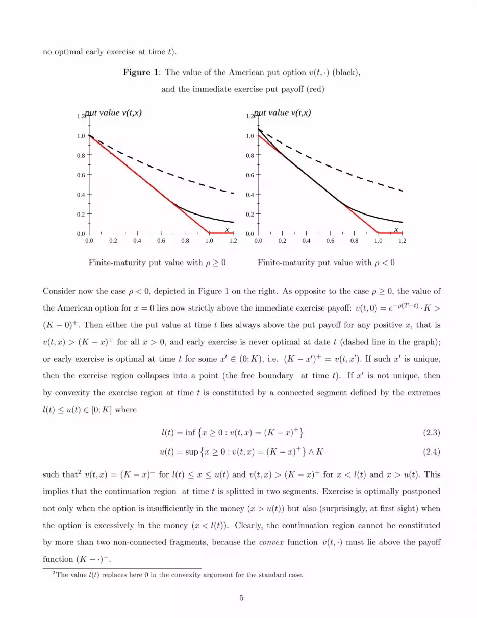
no optimal early exercise at time t).

Figure 1: The value of the American put option v(t; �) (black),

and the immediate exercise put payo¤ (red)

0.0 0.2 0.4 0.6 0.8 1.0 1.20.0

0.2

0.4

0.6

0.8

1.0

1.2put value v(t,x)

x

Finite-maturity put value with � � 0

0.0 0.2 0.4 0.6 0.8 1.0 1.20.0

0.2

0.4

0.6

0.8

1.0

1.2put value v(t,x)

x

Finite-maturity put value with � < 0

Consider now the case � < 0; depicted in Figure 1 on the right. As opposite to the case � � 0; the value of

the American option for x = 0 lies now strictly above the immediate exercise payo¤: v(t; 0) = e��(T�t) �K >

(K � 0)+: Then either the put value at time t lies always above the put payo¤ for any positive x, that is

v(t; x) > (K � x)+ for all x > 0; and early exercise is never optimal at date t (dashed line in the graph);

or early exercise is optimal at time t for some x0 2 (0;K), i.e. (K � x0)+ = v(t; x0): If such x0 is unique,

then the exercise region collapses into a point (the free boundary at time t). If x0 is not unique, then

by convexity the exercise region at time t is constituted by a connected segment de�ned by the extremes

l(t) � u(t) 2 [0;K] where

l(t) = inf�x � 0 : v(t; x) = (K � x)+

(2.3)

u(t) = sup�x � 0 : v(t; x) = (K � x)+

^K (2.4)

such that2 v(t; x) = (K � x)+ for l(t) � x � u(t) and v(t; x) > (K � x)+ for x < l(t) and x > u(t): This

implies that the continuation region at time t is splitted in two segments. Exercise is optimally postponed

not only when the option is insu¢ ciently in the money (x > u(t)) but also (surprisingly, at �rst sight) when

the option is excessively in the money (x < l(t)). Clearly, the continuation region cannot be constituted

by more than two non-connected fragments, because the convex function v(t; �) must lie above the payo¤

function (K � �)+:2The value l(t) replaces here 0 in the convexity argument for the standard case.

5

Let us denote with

ER =�(t; x) 2 [0;T ]� [0;+1[ : v(t; x) = (K � x)+

the (early) exercise region, and with

CR =�(t; x) 2 [0;T ]� [0;+1[ : v(t; x) > (K � x)+

the continuation region.

When the maturity is �nite and the interest rate is negative, we provide an accurate description of the

double continuation region separated from the (single) early exercise region by a double free boundary (see

Theorems 2.3 and 2.4). Such a �nding contributes to the extant literature on multiple free boundaries that

separate the (single) continuation region from the multiple exercise region for certain American options with

multiple assets, e.g. Broadie and Detemple (1997) and Villeneuve (1999).

The function v in (2:1) can be characterized as the solution of the variational inequality (see for instance

Bensoussan and Lions (1982))8>>>>>>><>>>>>>>:

v (T; �) = � (�)

v (t; �) � � (�) for any t 2 [0;T ]@@tv + Lv � �v � 0 on (0;T )�<

+

@@tv + Lv � �v = 0 on f(t; x) 2 (0;T )�<

+ : v (t; x) > �(x)g

(2.5)

where

� (x) = (K � x)+

(Lv)(t; x) = 1

2�2x2

@2

@x2v(t; x) + �x

@

@xv(t; x):

Such system of variational inequalities can be stated in Sobolev spaces (as in Bensoussan and Lions (1982)),

proving existence of the solution, and arguing uniqueness of such solution via a probabilistic argument

(veri�cation theorem). The same system of variational inequalities can be tackled by means of viscosity

solutions, showing that the probabilistic solution is a viscosity solution of the variational inequality, and

proving via analytic arguments the uniqueness of such solution (as, for instance, in Pham (1997)). Lamberton

(1998) characterizes the American put option as the solution of the variational inequality (2:5) to be read in

the distribution sense3. When interest rates are non-negative, it is well known that the variational inequality

(2:5) admits a smooth solution (see Jaillet, Lamberton and Lapeyre (1990) or Lamberton (1998)). The same

3Lamberton and Mikou (2008) have recently extended the analysis to the case of an exponential Lévy underlying when the

interest rate is positive.

6

conclusion can be achieved even if the interest rate is negative. In the next proposition we provide a precise

statement of this result. It can be proved by replicating the same proof of Theorem 3.6 and Corollary 3.7

in Jaillet, Lamberton and Lapeyre (1990), observing that when interest rates are negative, i.e. for � < 0;

the discount factor is positive and bounded by e��T :

Proposition 2.1 (Smoothness of the put value v, negative interest rate) The solution of (2:5)

admits partial derivatives @v@t ;

@v@x ;

@2v@x2

that are locally bounded on [0;T ) � <+: Moreover, v enjoys the

smooth-�t property, i.e. @v@x is continuous on [0;T )�<

+.

In the in�nite-maturity case, the constant double free boundary can be explicitly computed, by solving

the PDE entailed in (2:5) in the continuation region, and imposing smooth-pasting at the free boundary

(see Battauz, De Donno and Sbuelz (2010)). The result requires an ad-hoc direct veri�cation, because v1

violates the usual boundedness requirements4. Battauz, De Donno, and Sbuelz (2010) derived the perpetual

closed form solution for the special case of the real option problem. In the following proposition, we adapt

their statement to our current framework. The proof follows their same arguments, but, for convenience of

the reader, we recall the main steps in the appendix.

Proposition 2.2 (Perpetual put, negative interest rate) If T = +1;

� < 0; �� �2

2> 0 (2.6)

and ��� �

2

2

�2+ 2��2 > 0; (2.7)

then the perpetual American put option value is

v1(x) =

8>>>><>>>>:Al � x�l for x 2 (0; l1)

K � x for x 2 [l1;u1]

Au � x�u for x 2 (u1; +1)

(2.8)

where �u < �l are the negative solutions of the equation

1

2�2�2 +

��� �

2

2

�� � � = 0; (2.9)

that is

�l =���� �2

2

�+

r��� �2

2

�2+ 2��2

�2

4When � < 0 and x = 0 the optimal time to exercise is �� = +1, and the value of the American option is v1(0) =

Ehe���

�(K � 0)+

i= +1:

7

�u =���� �2

2

��r�

�� �2

2

�2+ 2��2

�2:

The critical asset prices are

l1; u1 = K�i

�i � 1for i = l; u (2.10)

and the constant Al and Au are given by

Al = �(l1)

1��l

�land Au = �

(u1)1��u

�u(2.11)

We now explain the role of conditions (2:6) and (2:7) of Proposition 2.2. In the case of negative interest

rates � < 0; the positive-drift condition (2:6) and the positive-discriminant condition (2:7) guarantee the

existence of (negative) solutions of equation (2:9) and rule out the potential explosive e¤ect of a negative

interest rate on the put value function. If the interest rate is deeply negative, the holder of the option may

obtain an in�nite expected gain by deferring inde�nitely the exercise of the option. This is unfeasible if the

possibility that the option goes out of the money as time goes by is signi�cant, i.e. if the growth rate of the

underlying asset X is high enough compared to the absolute value of the negative interest rate.

Such balance is reached exactly when condition (2:7) is satis�ed, i.e. if

j�j <

��� �2

2

�22�2

:

The function v de�ned in (2:8) enjoys the following properties in the continuation region: v is decreasing,

dominates the immediate payo¤, and the process�v(X(t))e��t

tis a martingale. The same condition

controls also for the supermartingality property of the process�v(X(t))e��t

tin the early exercise region.

In Theorem 2.3 we study the American put option problem with negative interest rates when the maturity

is �nite. In particular, we analyze the free boundary, which is constituted by two branches: the upper

free boundary, corresponding to the critical value u1 in the perpetual case, and the lower free boundary,

corresponding to l1 in the perpetual case. The upper free boundary enjoys all the property it has in the

standard case, where interest rates are positive: it is increasing, continuous and tends to the strike price at

maturity. The lower free boundary is decreasing, continuous everywhere but at maturity, where it displays

a discontinuity. We use the variational inequality approach (e.g. Jaillet, Lamberton and Lapeyre, 1990)

to prove the continuity of the double free boundary, thus extending the positive-interest-rate results5 of

Lamberton (1998).

5Given a positive interest rate, Lamberton and Mikou (2008) and Chevalier (2005) obtain similar results in the case of an

exponential Lévy underlying and of a local volatility underlying, respectively.

8

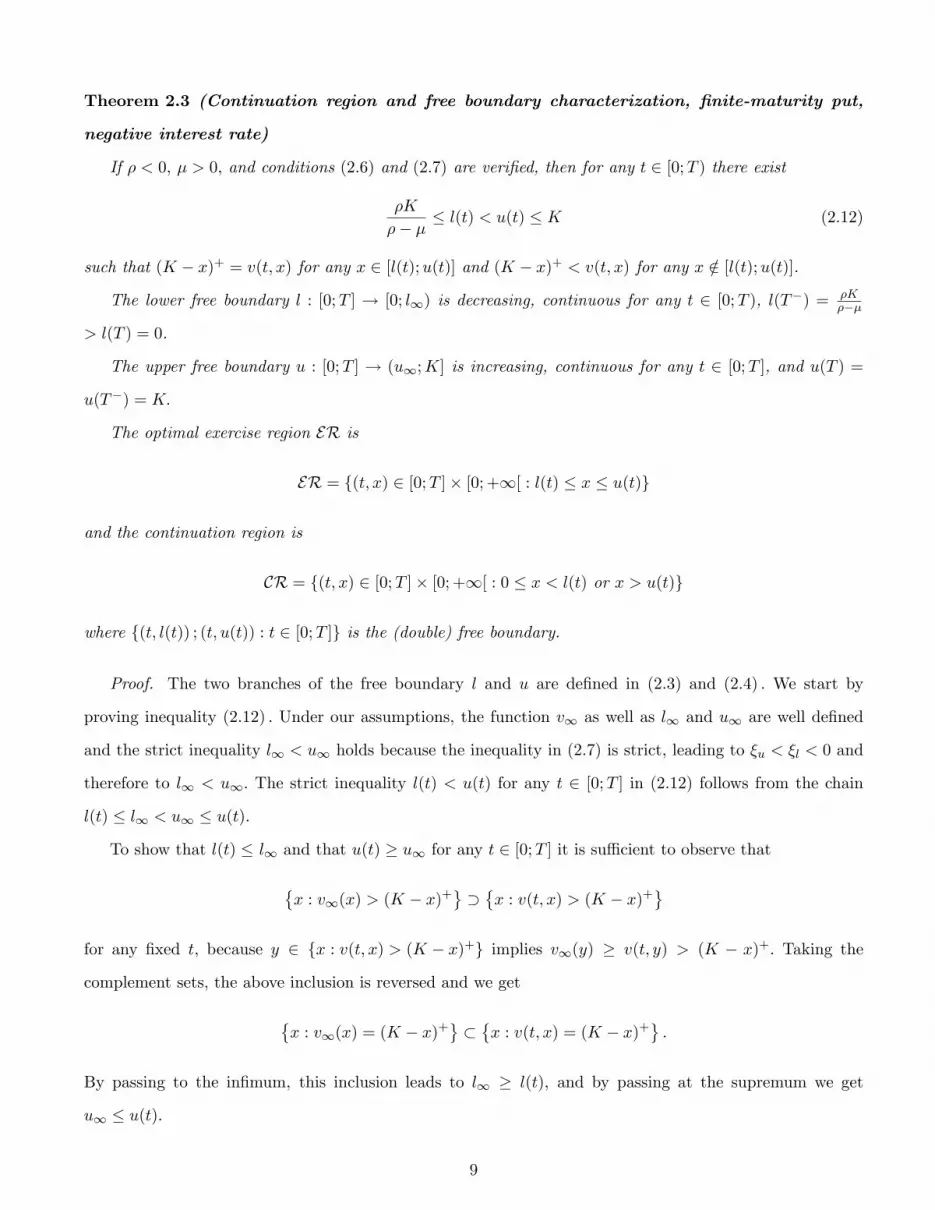
Theorem 2.3 (Continuation region and free boundary characterization, �nite-maturity put,

negative interest rate)

If � < 0; � > 0; and conditions (2:6) and (2:7) are veri�ed, then for any t 2 [0;T ) there exist

�K

�� � � l(t) < u(t) � K (2.12)

such that (K � x)+ = v(t; x) for any x 2 [l(t);u(t)] and (K � x)+ < v(t; x) for any x =2 [l(t);u(t)].

The lower free boundary l : [0;T ] ! [0; l1) is decreasing, continuous for any t 2 [0;T ), l(T�) = �K���

> l(T ) = 0.

The upper free boundary u : [0;T ] ! (u1;K] is increasing, continuous for any t 2 [0;T ], and u(T ) =

u(T�) = K:

The optimal exercise region ER is

ER = f(t; x) 2 [0;T ]� [0;+1[ : l(t) � x � u(t)g

and the continuation region is

CR = f(t; x) 2 [0;T ]� [0;+1[ : 0 � x < l(t) or x > u(t)g

where f(t; l(t)) ; (t; u(t)) : t 2 [0;T ]g is the (double) free boundary.

Proof. The two branches of the free boundary l and u are de�ned in (2:3) and (2:4) : We start by

proving inequality (2:12) : Under our assumptions, the function v1 as well as l1 and u1 are well de�ned

and the strict inequality l1 < u1 holds because the inequality in (2:7) is strict, leading to �u < �l < 0 and

therefore to l1 < u1: The strict inequality l(t) < u(t) for any t 2 [0;T ] in (2:12) follows from the chain

l(t) � l1 < u1 � u(t).

To show that l(t) � l1 and that u(t) � u1 for any t 2 [0;T ] it is su¢ cient to observe that

�x : v1(x) > (K � x)+

��x : v(t; x) > (K � x)+

for any �xed t; because y 2 fx : v(t; x) > (K � x)+g implies v1(y) � v(t; y) > (K � x)+: Taking the

complement sets, the above inclusion is reversed and we get

�x : v1(x) = (K � x)+

��x : v(t; x) = (K � x)+

:

By passing to the in�mum, this inclusion leads to l1 � l(t), and by passing at the supremum we get

u1 � u(t):

9

Next, we prove that

l(t) � �K

�� � for any t 2 [0;T ) :

We observe that any (t; x) in the exercise region ER satis�es the inequality

@

@tv + Lv � �v � 0

in (2:5) : Since for (t; x) 2 ER we have v(t; x) = K � x; the inequality simpli�es to

��x� � (K � x) = (�� �)x� �K � 0

that is

x � �K

�� � > 0 for any (t; x) 2 ER:

By passing to the in�mum over x for any �xed t in the previous inequality we get that l(t) � �K��� :

We now prove the monotonicity properties of l and u: We �rst show that l is decreasing. Let t0 < t00:

We have (K � l (t0))+ � v (t00; l (t0)) � v(t0; l (t0)) = (K � l (t0))+ ; where the �rst inequality follows from

v(t00; �) � (K � �)+ ; the second one from the fact that v(�; l (t0)) is decreasing, and the last equality from the

de�nition of l (t0) : As a consequence v (t00; l (t0)) = (K � l (t0))+ ; and therefore l (t00) � l (t0) :

To show that u is increasing, let t0 < t00: We exploit the monotonicity properties of v and we get

(K � u (t0))+ = v (t0; u (t0)) � v(t00; u (t0)) � (K � u (t0))+ : Therefore v(t00; u (t0)) = (K � u (t0))+ ; and,

consequently, u (t00) � u (t0) :

The next step is to prove that at maturity l (T ) = 0 and u (T ) = K. To show that l (T ) = 0; we observe

that since v(T; x) = (K � x)+

l(T ) = inf�x � 0 : v(T; x) = (K � x)+

= inf fx � 0g = 0:

The other equality, u (T ) = K; follows from

u(T ) = sup�x � 0 : v(T; x) = (K � x)+

^K = sup fx � 0g ^K = K:

We now show that u (T�) = K = u (T ) and l (T�) = �K��� > 0 = l (T ) : By construction u (t) � K for all

t 2 [0;T ] ; and hence u (T�) � K: Suppose by contradiction that u (T�) < K: The set (0;T )�(u (T�) ;K) �

CR and therefore

(L � �) v = � @@tv � 0 .

As t " T we have

(L � �) v ! (L � �) (K � x) = (�� �)x� �K for x 2�u�T��;K�;

10

where the limit is in the sense of distributions. But then we have (��+ �)x+ �K � 0 for x 2 (u (T�) ;K)

and therefore

(��+ �)x+ �K � (��+ �)K + �K � �K � 0

delivering the contradiction.

Suppose now (by contradiction) that l (T�) > �K��� : The set (0;T )� (0; l (T

�)) � CR and hence

(L � �) v = � @@tv � 0 for x 2

��K

�� � ; l�T�����0; l�T���:

As t " T we have

(L � �) v ! (L � �) (K � x) = (�� �)x� �K for x 2��K

�� � ; l�T���;

where the limit is in the sense of distributions. We hence have

(�� �)x� �K � 0 for x 2��K

�� � ; l�T���

that is

(��+ �)x+ �K � 0 for x 2��K

�� � ; l�T���:

which delivers the contradiction because x � �K��� implies

(��+ �)x+ �K � (��+ �) �K�� � + �K = 0:

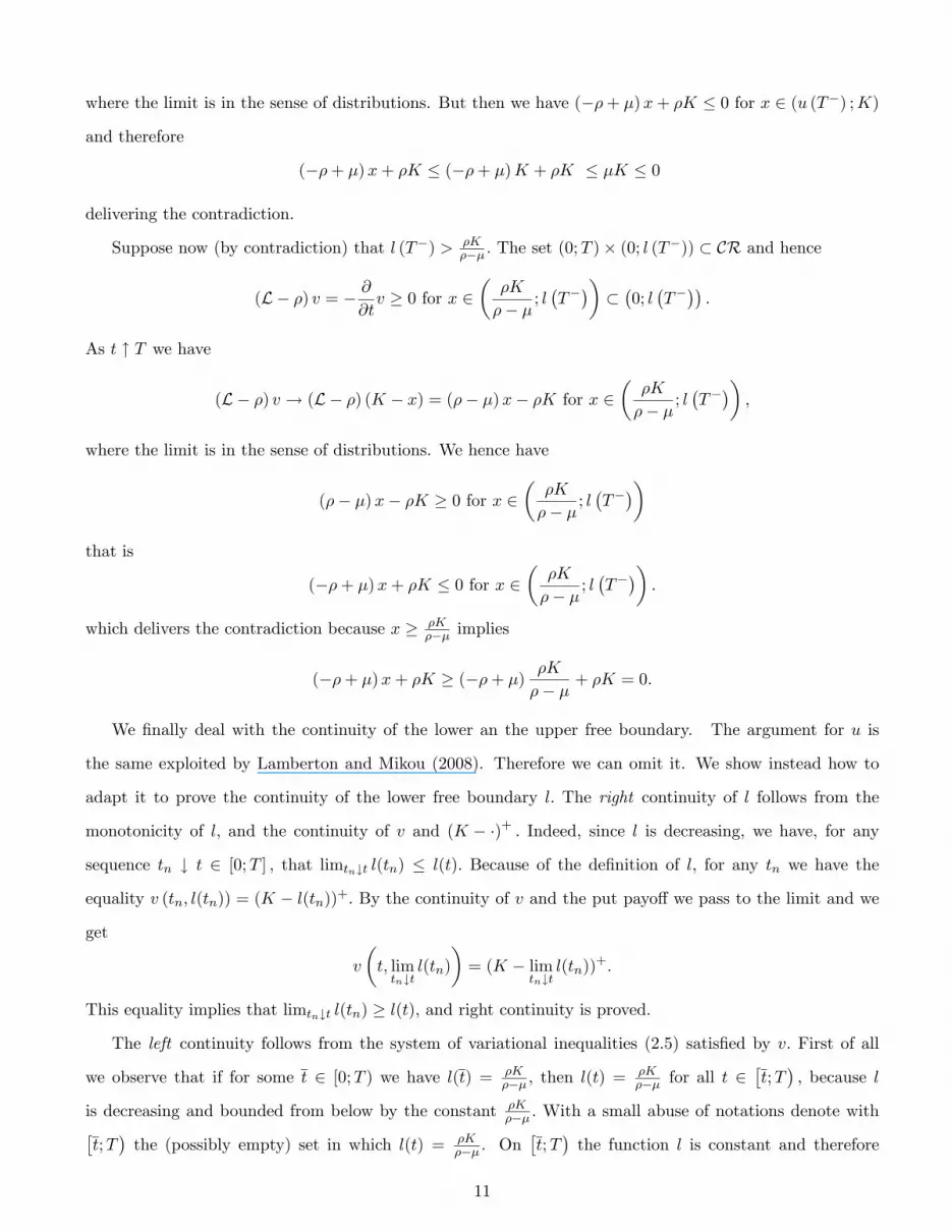
We �nally deal with the continuity of the lower an the upper free boundary. The argument for u is

the same exploited by Lamberton and Mikou (2008). Therefore we can omit it. We show instead how to

adapt it to prove the continuity of the lower free boundary l: The right continuity of l follows from the

monotonicity of l; and the continuity of v and (K � �)+ : Indeed, since l is decreasing, we have, for any

sequence tn # t 2 [0;T ] ; that limtn#t l(tn) � l(t): Because of the de�nition of l; for any tn we have the

equality v (tn; l(tn)) = (K � l(tn))+: By the continuity of v and the put payo¤ we pass to the limit and we

get

v

�t; limtn#t

l(tn)

�= (K � lim

tn#tl(tn))

+:

This equality implies that limtn#t l(tn) � l(t); and right continuity is proved.

The left continuity follows from the system of variational inequalities (2:5) satis�ed by v: First of all

we observe that if for some t 2 [0;T ) we have l(t) = �K��� ; then l(t) =

�K��� for all t 2

�t;T�; because l

is decreasing and bounded from below by the constant �K��� : With a small abuse of notations denote with�

t;T�the (possibly empty) set in which l(t) = �K

��� . On�t;T�the function l is constant and therefore

11

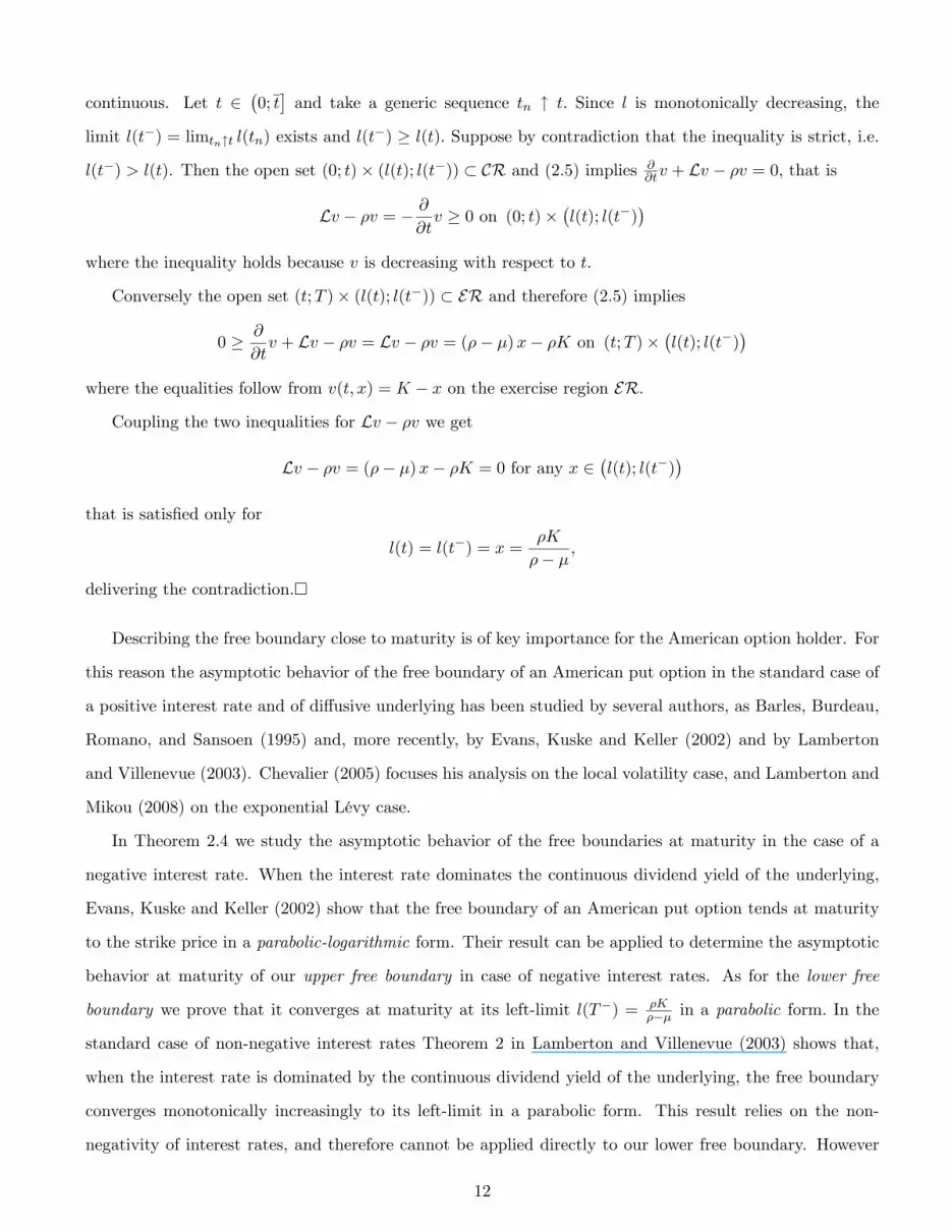
continuous. Let t 2�0; t�and take a generic sequence tn " t: Since l is monotonically decreasing, the

limit l(t�) = limtn"t l(tn) exists and l(t�) � l(t): Suppose by contradiction that the inequality is strict, i.e.

l(t�) > l(t). Then the open set (0; t)� (l(t); l(t�)) � CR and (2:5) implies @@tv + Lv � �v = 0; that is

Lv � �v = � @@tv � 0 on (0; t)�

�l(t); l(t�)

�where the inequality holds because v is decreasing with respect to t:

Conversely the open set (t;T )� (l(t); l(t�)) � ER and therefore (2:5) implies

0 � @

@tv + Lv � �v = Lv � �v = (�� �)x� �K on (t;T )�

�l(t); l(t�)

�where the equalities follow from v(t; x) = K � x on the exercise region ER.

Coupling the two inequalities for Lv � �v we get

Lv � �v = (�� �)x� �K = 0 for any x 2�l(t); l(t�)

�that is satis�ed only for

l(t) = l(t�) = x =�K

�� �;

delivering the contradiction.�

Describing the free boundary close to maturity is of key importance for the American option holder. For

this reason the asymptotic behavior of the free boundary of an American put option in the standard case of

a positive interest rate and of di¤usive underlying has been studied by several authors, as Barles, Burdeau,

Romano, and Sansoen (1995) and, more recently, by Evans, Kuske and Keller (2002) and by Lamberton

and Villenevue (2003). Chevalier (2005) focuses his analysis on the local volatility case, and Lamberton and

Mikou (2008) on the exponential Lévy case.

In Theorem 2.4 we study the asymptotic behavior of the free boundaries at maturity in the case of a

negative interest rate. When the interest rate dominates the continuous dividend yield of the underlying,

Evans, Kuske and Keller (2002) show that the free boundary of an American put option tends at maturity

to the strike price in a parabolic-logarithmic form. Their result can be applied to determine the asymptotic

behavior at maturity of our upper free boundary in case of negative interest rates. As for the lower free

boundary we prove that it converges at maturity at its left-limit l(T�) = �K��� in a parabolic form. In the

standard case of non-negative interest rates Theorem 2 in Lamberton and Villenevue (2003) shows that,

when the interest rate is dominated by the continuous dividend yield of the underlying, the free boundary

converges monotonically increasingly to its left-limit in a parabolic form. This result relies on the non-

negativity of interest rates, and therefore cannot be applied directly to our lower free boundary. However

12

Lamberton and Villenevue (2003) provide an expansion result for value functions (Theorem 1 and Remark

2) that enables us to show that under our assumptions the lower free boundary converges monotonically

decreasingly to its left-limit in a parabolic form.

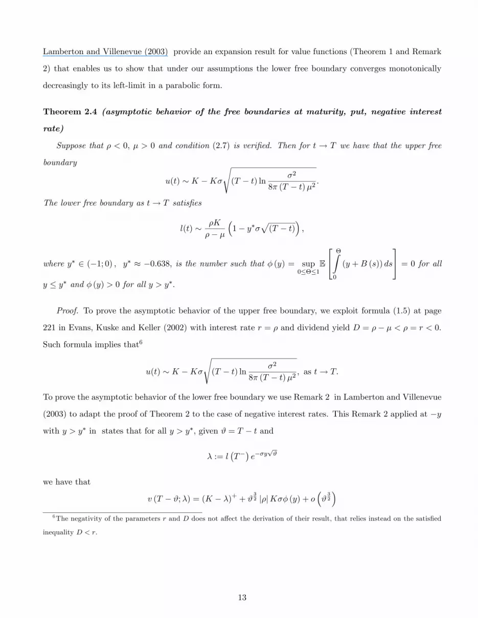
Theorem 2.4 (asymptotic behavior of the free boundaries at maturity, put, negative interest

rate)

Suppose that � < 0; � > 0 and condition (2:7) is veri�ed. Then for t ! T we have that the upper free

boundary

u(t) � K �K�

s(T � t) ln �2

8� (T � t)�2 :

The lower free boundary as t! T satis�es

l(t) � �K

�� �

�1� y��

p(T � t)

�;

where y� 2 (�1; 0) ; y� � �0:638; is the number such that � (y) = sup0���1

E

24 �Z0

(y +B (s)) ds

35 = 0 for ally � y� and � (y) > 0 for all y > y�:

Proof. To prove the asymptotic behavior of the upper free boundary, we exploit formula (1.5) at page

221 in Evans, Kuske and Keller (2002) with interest rate r = � and dividend yield D = �� � < � = r < 0:

Such formula implies that6

u(t) � K �K�

s(T � t) ln �2

8� (T � t)�2 ; as t! T:

To prove the asymptotic behavior of the lower free boundary we use Remark 2 in Lamberton and Villenevue

(2003) to adapt the proof of Theorem 2 to the case of negative interest rates. This Remark 2 applied at �y

with y > y� in states that for all y > y�; given # = T � t and

� := l�T��e��y

p#

we have that

v (T � #;�) = (K � �)+ + #32 j�jK�� (y) + o

�#32

�6The negativity of the parameters r and D does not a¤ect the derivation of their result, that relies instead on the satis�ed

inequality D < r.

13

since @@x

���Ke��t + (�� �) e�

����+�2

2

�t+�x

��0; 1� ln

�K���

�= �K� < 0: This equation7 substitutes equa-

tion (2) in the proof of Theorem 2 in Lamberton and Villenevue (2003). Since � (y) > 0; it follows that

v (T � #;�) > (K � �)+ :

Hence (T � #;�) =�T � #; l (T�) e��y

p#�2 CR and for # small enough this is equivalent to say that

� = l�T��e��y

p# < l (T � #) :

Note that the inequality is here reversed with respect to the standard case of unique (upper) free boundary.

Passing to the log we get

ln l�T��� �y

p# < ln l (T � #)

ln l�T��� ln l (T � #) < �y

p#

and therefore

lim supt!T

l (T�)� l (t)l (T�)�

p(T � t)

� y:

Since the inequality holds for all y > y�; y ! y� we get

lim supt!T

l (T�)� l (t)l (T�)�

p(T � t)

� y�:

This means that

l (t) � l�T�� �1� y��

p(T � t)

�for t! T:

We now prove the opposite inequality for y � y�. If for all y � y� and # = T � t! 0

l (T � #) � l�T��e��y

p# � l

�T�� �1� y�

p#�

the proof is complete. Hence, suppose now that

l (T � #) > � = l�T��e��y

p#:

This means that (T � #;�) 2 CR: We exploit Remark 2 in Lamberton and Villenevue (2003) applied to �y

(instead of y) that implies

' (#) = v (T � #;�) = (K � �)+ + g (#) with g (#) = o�#32

�> 0:

7With the notation of Theorem 2 in Lamberton and Villenevue (2003) r = �; � = � � �; t0 = 0; x0 =1�ln �K

��� ; f(t; x) =

e��t

K � e

����2

2

�t+�x

!+, Df (t; x) = ��Ke��t + (�� �) e

�����+�2

2

�t+�x

.

14

The smooth �t property (Proposition 2.1) allows to �nd � 2 (�; l (T � #)) such that

v (T � #;�)� (K � �) = (l (T � #)� �)2

2

@2v

@x2(T � #; �) (2.13)

Indeed, since v admits continuous �rst order derivative w.r.t. x and there exists @2v@x2

(T � #;x) for all

x 2 (�; l (T � #)) ; we can apply Taylor expansion with the Lagrange remainder for x = � and bx0 = l (T � #)to conclude that

v (T � #;x) = v (T � #; bx0) + @

@xv (T � #; bx0) (x� bx0) + 1

2

@2v

@x2(T � #; �) (x� bx0)2

for some � 2 (x; bx0) = (�; l (T � #)) : Sincev (T � #; bx0) = v (T � #; l (T � #)) = K � l (T � #)

@

@xv (T � #; bx0) = @

@xv (T � #; l (T � #)) = �1

the Taylor expansion delivers (2:13) :

Since � 2 (�; l (T � #)) ; we have that (T � #; �) 2 CR and therefore

� @

@#v + Lv � �v = 0 for (t; x) = (T � #; �)

with (Lv)(t; x) = 12�

2x2 @2

@x2v(t; x) + �x @

@xv(t; x): From the PDE at (t; x) = (T � #; �) we derive that

1

2�2�2

@2v

@x2(T � #; �) = @

@#v (T � #; �)� �� @

@xv (T � #; �) + �v (T � #; �)

� 0� �� @

@xv (T � #; �) + �v (T � #; �) because v increasing w.r.t. #

> ��� (�1) + �v (T � #; �) because @

@xv (T � #; �) � �1

> �� + �v (T � #;�) because � > � and v (T � #; �) < v (T � #;�)

where ��+ �v (T � #;�) > 0: Therefore

(l (T � #)� �)2 = (v (T � #;�)� (K � �))12@2v@x2

(T � #; �)

<g (#)

��+�v(T�#;�)�2�2

=�2�2g (#)

��+ � ((K � �) + g (#)) < Cg (#)

��+ � ((K � �) + g (#))

The denominator can be rewritten as

��+ � ((K � �) + g (#)) = (�� �)�+ �K + g (#)

= (�� �) �K�� �e

��yp# + �K + g (#)

= �K�1� e��y

p#�+ g (#) � �K�y

p#+ o

��yp#�

15

Therefore

(l (T � #)� �)2 < C g (#)

�K�1� e��y

p#�+ g (#)

� Co�#32

��K�y

p#+ o

��yp#� = C 0 o

�#32

���y

p#+ o

��yp#� = C 0o ��2y2#�

with C;C 0 > 0: This implies that

(l (T � #)� �) < o���y

p#�as #! 0

But then

l (T � #)� � = l (T � #)� l�T��e��y

p# < o

���y

p#�as #! 0

i.e.

l (T � #) � l�T�� �1� �y

p#�+ o

���y

p#�as #! 0

for y � y�: In other words

l�T��� l (t) � l

�T����l�T�� �1� y�

p(T � t)

��= l�T��y�p(T � t);

for all y � y�; and hence

l�T��� l (t) � l

�T��y��p(T � t):

Therefore we get

lim inft!T

l (T�)� l (t)l (T�)�

p(T � t)

� y�

and thus our proof is complete.�

In Figure 2 we plot the double free boundary for an American put option with a negative interest rate.

The dashed part of the upper free boundary is obtained via binomial approximation. The solid lines are

plotted from the asymptotic approximation8.

8The binomial approximation of the lower free boundary coincides numerically with the parabolic asymptotic approximation

for the entire life of the option.

16

Figure 2: Double free boundary for an American put option with

� = �4%; K = 1:2; � = 20%; � = 8%; T = 1:

0.0 0.2 0.4 0.6 0.8 1.00.0

0.2

0.4

0.6

0.8

1.0

1.2

1.4

l

oo

oo

u

l(t)

u(t)

x

tT=

CONTINUATION REGION

CONTINUATION REGION

EXERCISE

K

EARLY

REGION

Red (green) circles indicate the exercise (no exercise) regionat T .

3 The American call

In this section we consider an American call option written on the log-normal asset X; whose drift under

the valuation measure is �: We denote the volatility with �; the strike with K; and discount rate with �:

Our aim is to compute the value of the option at time t, given by

ess supt���T

Ehe��(��t) (X(�)�K)+

���Fti = v(t;X(t))where

v(t; x) = sup0���T�t

E

"e���

�x � exp

���� �

2

2

��+ � B(�)

��K

�+#(3.1)

where B is a standard Brownian motion under the valuation measure. We analyze the American call option

problem in the case of a negative interest rate �.

If the drift of S is positive, � > 0; the value of the perpetual call option when interest rates are negative

is clearly unbounded. In fact

v(t; x) = v1(x) = sup0��

E

"e���

�x � exp

���� �

2

2

��+ � B(�)

��K

�+#

� sup0�T

e��T ��E�x � exp

���� �

2

2

�T + � B(T )

���K

�+= sup0�T

e��T�x � e�T �K

�+= +1

17

by applying Jensen�s inequality.

On the contrary, for �; � < 0, problem (3:1) can be bounded also in the perpetual case, as we show in

Proposition 3.2. In the �nite-maturity case, the function v in (3:1) can be characterized as the solution of

the variational inequality (2:5) with � (x) = (x�K)+:

We recall that the function v in (3:1) has the following properties, regardless of the sign of � : v dominates the

call immediate payo¤, i.e. 0 � (x�K)+ � v(t; x) for any t 2 [0;T ] and x � 0: Moreover for any t 2 [0;T ] ;

the function v(t; x) is convex and increasing with respect to x: These properties are inherited from convexity

and monotonicity of the immediate call payo¤. From the de�nition of v in (3:1) as a supremum on the

set of stopping times from 0 up to time-to-maturity we can also deduce that for any x � 0; the function

v(t; x) is decreasing with respect to t: Finally, the �nite-maturity option is dominated by the perpetual

one: v(t; x) � v1(x) for any t 2 [0;T ] and x � 0: We also observe that the negative sign of � and � with

� < � < 0 prevents the function v1 to be dominated by the identity function, i.e. the inequality v1(x) � x

does not hold true, as opposite to the case depicted in Xia and Zhou (2007).

Because of the previous properties of v, the exercise region at time t is constituted by a connected

segment de�ned by the extremes l(t) � u(t) 2 [0;K] where

l(t) = inf�x � 0 : v(t; x) = (x�K)+

^K

u(t) = sup�x � 0 : v(t; x) = (x�K)+

such that v(t; x) = (x�K)+ for l(t) � x � u(t) and v(t; x) > (x�K)+ for x < l(t) and x > u(t): This implies

that the continuation region at time t is splitted in two segments, as for the put case. We characterize

the continuation and exercise region, and the free boundary in Theorem 3.3. In Proposition 3.2 we give

parameter value restrictions under which the American perpetual call option is �nite even when interest

rates are negative. We also provide explicit expressions for the constant double free boundary.

In the �nite-maturity case the lower free boundary enjoys all the property it has in the standard case,

where interest rates are positive: it is decreasing, continuous and tends to the strike price at maturity. The

upper free boundary is increasing, continuous everywhere but at maturity, where it is in�nite.

Proposition 3.2 and Theorem 3.3 are proved by exploiting (respectively) Proposition 2.2 and Theorem

2.3, and by applying the American put-call symmetry (see P. Carr and M. Chesney (1996), and M. Schroder

(1999)). The American put-call symmetry relates the price of an American call option to the price of an

American put option by swapping the initial underlying stock price with the strike price, and the dividend

yield with the interest rate. As explained by Detemple (2001), such symmetry relies on the symmetry of the

distribution of the log-price of X; and on the symmetry of call and put payo¤s. The change of numeraire

18

allows to derive such property also in our case, where both the interest rate � and the �dividend yield�

� = �� � are negative. The negativity of both the interest rate � and �dividend yield� � = �� � is crucial

to determine the presence of the double continuation region. For the ease of the reader, we state here the

American put-call symmetry in our notations, and then our Proposition 3.2 and Theorem 3.3 with the

characterization of the free boundary for an American call option in case of a negative interest rate.

Proposition 3.1 (American put-call symmetry)

Consider the American call option with strike K; interest rate �; underlying�s drift �; underlying�s

volatility �; and initial underlying�s value x; whose value at time t 2 [0;T ] is denoted with v (t; x) =

vcall (t; x;K; �; �; �) :

Consider the symmetric American put option with strike Kput = x; interest rate �put = ���, underlying�s

drift �put = ��; underlying�s volatility �put = � and initial underlying�s value xput = K; whose value at

time t 2 [0;T ] is denoted with vput (t; xput;Kput; �put; �put; �put) = vput (t;K;x; �� �; ��; �) :

1. The following conditions

� < � < ��2

2< 0; (3.2)�

�� �2

2

�2+ 2��2 > 0; (3.3)

for �; �; � in the American call problem are equivalent to conditions (2:6) and (2:7) for parameters

�put; �put; �put in the symmetric American put problem.

2. (Carr and Chesney, 1996; Detemple, 2001; Detemple 2006))The value of the American call coincides

with the value of the symmetric American put

v (t; x) = vcall (t; x;K; �; �; �) = vput (t;K;x; �� �; ��; �) (3.4)

for any t 2 [0;T ] :

3. For any t 2 [0;T ] let l (t) (resp. u (t)) denote the lower (resp. upper) critical price at time t for the

American call option with strike K; and parameters �; �; �. Let lput (t) (resp. uput (t)) denote the

lower (resp. upper) critical price at time t for the symmetric American put with strike Kput = 1; and

parameters �put; �put; �put:If (3:2) and (3:3) are satis�ed, then for any t 2 [0;T ] we have

l (t) =K

uput (t)(3.5)

u (t) =K

lput (t)(3.6)

19

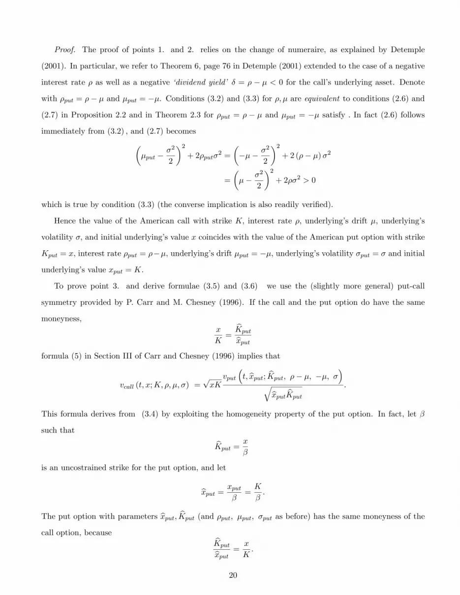
Proof. The proof of points 1. and 2. relies on the change of numeraire, as explained by Detemple

(2001). In particular, we refer to Theorem 6, page 76 in Detemple (2001) extended to the case of a negative

interest rate � as well as a negative �dividend yield� � = � � � < 0 for the call�s underlying asset. Denote

with �put = �� � and �put = ��. Conditions (3:2) and (3:3) for �; � are equivalent to conditions (2:6) and

(2:7) in Proposition 2:2 and in Theorem 2:3 for �put = � � � and �put = �� satisfy : In fact (2:6) follows

immediately from (3:2) ; and (2:7) becomes��put �

�2

2

�2+ 2�put�

2 =

���� �

2

2

�2+ 2 (�� �)�2

=

��� �

2

2

�2+ 2��2 > 0

which is true by condition (3:3) (the converse implication is also readily veri�ed).

Hence the value of the American call with strike K; interest rate �; underlying�s drift �; underlying�s

volatility �; and initial underlying�s value x coincides with the value of the American put option with strike

Kput = x; interest rate �put = ���, underlying�s drift �put = ��; underlying�s volatility �put = � and initial

underlying�s value xput = K.

To prove point 3. and derive formulae (3:5) and (3:6) we use the (slightly more general) put-call

symmetry provided by P. Carr and M. Chesney (1996). If the call and the put option do have the same

moneyness,x

K=bKputbxput

formula (5) in Section III of Carr and Chesney (1996) implies that

vcall (t; x;K; �; �; �) =pxK

vput

�t; bxput; bKput; �� �; ��; ��qbxput bKput :

This formula derives from (3:4) by exploiting the homogeneity property of the put option. In fact, let �

such that bKput = x

�

is an uncostrained strike for the put option, and let

bxput = xput�

=K

�:

The put option with parameters bxput; bKput (and �put; �put; �put as before) has the same moneyness of thecall option, because bKputbxput = x

K:

20

Moreover

vcall (t; x;K; �; �; �) = vput (t; xput;Kput; �put; �put; �put) by formula (3:4)

= vput (t;K;x; �� �; ��; �)

= � � vput�t;K

�;x

�; �� �; ��; �

�homogeneity property of put

= � � vput�t; bxput; bKput; �put; �put; �put� :

Writing

� =p� � � =

sxbKput � Kbxput

we arrive at formula (5) in Section III of Carr and Chesney (1996). We apply now such formula to derive

the expression of the upper free boundary as in formula (3:6) : Since (2:6) and (2:7) in Proposition 2:2 and

in Theorem 2:3 are satis�ed, there exist two critical prices at time t 2 (0;T ) for the American put option

vput

�t; bxput; bKput; �put; �put; �put� : Let let bKput = 1; and denote with

0 < lput(t) < uput(t)

the lower and upper free boundary of the American put option vput (t; bxput; 1; �put; �put; �put) : The para-meters x;K ; and bxput are constrained by the equality

x

K=

1bxput :The Carr and Chesney version of the American put-call symmetry allows to write

vcall (t; x;K; �; �; �) =pxK

vput (t; bxput; 1; �� �; ��; �)p1 � bxput :

The time t upper critical boundary for the call can be written as

u(t) = sup�x � 0 : vcall(t; x) = (x�K)+

= sup

(Kbxput � 0 : pxK vput (t; bxput; 1; �� �; ��; �)pbxput =

�Kbxput �K

�+)

= K � inf

(bxput � 0 :s

KbxputKvput (t; bxput; 1; �� �; ��; �)pbxput =

�Kbxput �K

�+)!�1because

x

K=

1bxput= K �

�inf

�bxput � 0 : Kbxput vput (t; bxput; 1; �� �; ��; �) = Kbxput (1� bxput)+���1

= K ��inf�bxput � 0 : vput (t; bxput; 1; �� �; ��; �) = (1� bxput)+��1

= K � (lput (t))�1 ;

21

which gives formula (3:6) : Formula (3:5) follows by similar arguments. Formulae (3:5) and (3:6) are the

extension of formula (6) in Section III of Carr and Chesney (1996) to account for the double free boundary.�

We exploit Proposition 3.1 to study the double free boundary for the American call option. The next

proposition focuses on the perpetual case. Theorem 3.3 deals with the �nite-maturity case, and Theorem

3.4 provides the asymptotic behavior of the upper and lower free boundaries at maturity.

Proposition 3.2 (Perpetual call, negative interest rate) If T = +1; and conditions (3:2) and (3:3)

hold, then the perpetual American call option value is

v1(x) =

8>>>><>>>>:Al � x�l for x 2 (0; l1)

x�K for x 2 [l1;u1]

Au � x�u for x 2 (u1; +1)

where �l > �u > 1 are the positive solutions of the equation (2:9) : The critical asset prices are l1; u1 de�ned

in (2:10), and the constant Al and Au are given by equation (2:11) :

Proof. By exploiting the put-call symmetry, �put = ��� and �put = �� satisfy conditions (2:6) and (2:7)

in Proposition 2:2 (see Proposition 3.1). Therefore there exist two constant critical prices for the symmetric

perpetual put option

0 < lput1 < uput1 :

The prices lput1 < uput1 lead to u1 > l1 for the call option via equations (3:6) and (3:5) :�

Theorem 3.3 (Continuation region and free boundary characterization, �nte-maturity call,

negative interest rate)

Under conditions (3:2) and (3:3) ; for any t 2 [0;T ) there exist

l(t) � l1 < u1 � u(t)

such that (x�K)+ = v(t; x) for any x 2 [l(t);u(t)] and (x�K)+ < v(t; x) for any x =2 [l(t);u(t)].

The lower free boundary l : [0;T ] ! [K; l1) is decreasing, continuous for any t 2 [0;T ], and l(T ) =

l(T�) = K.

The upper free boundary u : [0;T ) !�u1;

�K���

iis increasing, continuous for any t 2 [0;T ), with

u(T�) = �K��� > K and u(T ) = +1:

The optimal exercise region ER is

ER = f(t; x) 2 [0;T ]� [0;+1[ : l(t) � x � u(t)g

22

and the continuation region is

CR = f(t; x) 2 [0;T ]� [0;+1[ : 0 � x < l(t) or x > u(t)g

where f(t; l(t)) ; (t; u(t)) : t 2 [0;T ]g is the free boundary.

Proof. Under assumptions (3:3) and (3:2), the function v1 as well as l1 and u1 are well de�ned. The

monotonicity properties of the free boundary as well as the continuity follow by similar arguments of the put

case. The results can be also be derived form Theorem 2.3, exploiting the American put-call symmetry as

explained in Proposition 3.1. We focus here on the (non standard) upper free boundary for the call option,

whose existence is implied by the negative interest rate � < 0. For t = T; the de�nition of u as

u(T ) = sup�x � 0 : v(T; x) = (x�K)+

implies

u(T ) = +1:

For any t 2 (0;T ) ; equation (3:6) in Proposition 3.1 yields that

u (t) =K

lput (t)

is positive, increasing and continuous, because by Theorem 2.3 the (non standard) lower critical price of

the put option lput is positive, decreasing and continuous on (0;T ) : In particular, the limit of u as t! T�

is

u�T��=

K

lput (T�)=

K�put

�put��put=

K(���)���+�

=K � ��� � > K

and this concludes the proof.�

Theorem 3.4 (asymptotic behavior of the free boundaries at maturity, call, negative interest

rate)

Suppose that � < 0; � > 0 and condition (2:7) is veri�ed. Then for t ! T we have that the upper free

boundary

u(t) � �K

�� �

�1 + y��

p(T � t)

�The lower free boundary for t! T satis�es

l(t) � K +K�

s(T � t) ln �2

8� (T � t)�2 ;

where y� � �0:638 is de�ned in Theorem 2.4.

23

Proof. The asymptotic expressions of u and l at maturity derive from formulae (3:5) and (3:6) applied

to the asymptotics found in Theorem 2:4 for the symmetric put with parameters as de�ned in Proposition

3.1. Taylor approximation of �rst order delivers the �nal expression.�

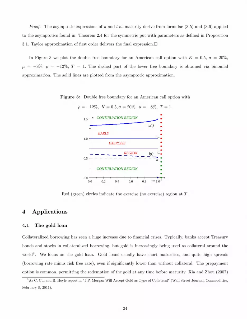
In Figure 3 we plot the double free boundary for an American call option with K = 0:5; � = 20%;

� = �8%; � = �12%; T = 1: The dashed part of the lower free boundary is obtained via binomial

approximation. The solid lines are plotted from the asymptotic approximation.

Figure 3: Double free boundary for an American call option with

� = �12%; K = 0:5; � = 20%; � = �8%; T = 1:

0.0 0.2 0.4 0.6 0.8 1.00.0

0.5

1.0

1.5

l

oo

oo

u

l(t)

u(t)

x

tT=

CONTINUATION REGION

CONTINUATION REGION

EXERCISE

K

EARLY

REGION

Red (green) circles indicate the exercise (no exercise) region at T .

4 Applications

4.1 The gold loan

Collateralized borrowing has seen a huge increase due to �nancial crises. Typically, banks accept Treasury

bonds and stocks in collateralized borrowing, but gold is increasingly being used as collateral around the

world9. We focus on the gold loan. Gold loans usually have short maturities, and quite high spreads

(borrowing rate minus risk free rate), even if signi�cantly lower than without collateral. The prepayment

option is common, permitting the redemption of the gold at any time before maturity. Xia and Zhou (2007)

9As C. Cui and R. Hoyle report in "J.P. Morgan Will Accept Gold as Type of Collateral" (Wall Street Journal, Commodities,

February 8, 2011).

24

focus on perpetual stock loans. Gold loans are di¤erent, because gold is a tradable investment asset with

storage and insurance costs and without payouts. This leads to peculiar redemption policies.

In a gold loan, the borrower receives at time 0 (the date of contract inception) the loan amount q > 0

using one mass unit (one troy ounce, say) of gold as collateral. This amount grows at the rate , where

is a constant loan interest rate (higher than the riskless interest rate r) stipulated in the contract, and

the cost of reimbursing the loan at time t is thus given by qe t. When paying back the loan, the borrower

regains the gold and the contract is terminated. We assume the costs of storing and insuring gold holdings

are Gu > 0 per unit of time, where G is the gold spot price. Consistently10, the dynamics of G under the

risk-neutral measure Q is assumed to be

dG(t)

G(t)= (r + u) dt+ �dW (t);

where r is the constant riskless rate, � is the gold returns�volatility, and W is a Brownian motion under

the risk-neutral measure Q. Given a �nite maturity T , the value of the redemption option at date 0 is

C(t; G (0)) = sup0���T

EQ�e�r� (G(�)� qe � )+

�= sup0���T

EQhe�(r� )� (X(�)� q)+

iwhere X(t) = G (t) e� t is the gold price de�ated at the rate : Therefore, the initial value of the redemption

option of a gold loan is the initial value of an American call option in (3:1) on the lognormal underlying X

with parameters

� = r � < 0

� = r + u�

K = q:

Similarly, the value of the redemption option at any date t 2 [0;T ] can be computed as C(t; G (t)) =

v(t;X (t)); with v de�ned in (3:1) : The gold holdings costs u are positive, but dominated by the spread

� r > 0; therefore � < � < 0: If conditions (3:2) and (3:3) are also veri�ed, i.e.

r � < r � + u < ��2

2and

�r � + u� �

2

2

�2+ 2�2 (r � ) > 0

a double no-redemption region appears in the perpetual case, as by Proposition 3.2. Using the same propo-

sition, we can compute the perpetual constant free boundaries l1 and u1 in terms of the de�ated gold

10See Hull (2011).

25

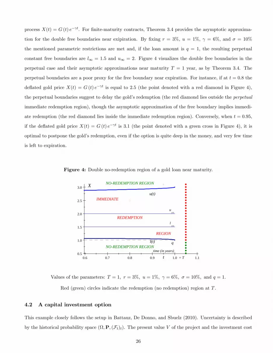
process X(t) = G (t) e� t. For �nite-maturity contracts, Theorem 3.4 provides the asymptotic approxima-

tion for the double free boundaries near exipiration. By �xing r = 3%, u = 1%, = 6%, and � = 10%

the mentioned parametric restrictions are met and, if the loan amount is q = 1, the resulting perpetual

constant free boundaries are l1 = 1:5 and u1 = 2. Figure 4 visualizes the double free boundaries in the

perpetual case and their asymptotic approximations near maturity T = 1 year, as by Theorem 3.4. The

perpetual boundaries are a poor proxy for the free boundary near expiration. For instance, if at t = 0:8 the

de�ated gold price X(t) = G (t) e� t is equal to 2:5 (the point denoted with a red diamond in Figure 4),

the perpetual boundaries suggest to delay the gold�s redemption (the red diamond lies outside the perpetual

immediate redemption region), though the asymptotic approximation of the free boundary implies immedi-

ate redemption (the red diamond lies inside the immediate redemption region). Conversely, when t = 0:95,

if the de�ated gold price X(t) = G (t) e� t is 3:1 (the point denoted with a green cross in Figure 4), it is

optimal to postpone the gold�s redemption, even if the option is quite deep in the money, and very few time

is left to expiration.

Figure 4: Double no-redemption region of a gold loan near maturity.

0.6 0.7 0.8 0.9 1.0 1.10.5

1.0

1.5

2.0

2.5

3.0

loo

oou

l(t)

u(t)

x

t = T

NO­REDEMPTION REGION

NO­REDEMPTION REGION

REDEMPTION

q

IMMEDIATE

REGION

X

time (in years)

Values of the parameters: T = 1; r = 3%; u = 1%; = 6%; � = 10%; and q = 1:

Red (green) circles indicate the redemption (no redemption) region at T .

4.2 A capital investment option

This example closely follows the setup in Battauz, De Donno, and Sbuelz (2010). Uncertainty is described

by the historical probability space (;P; (Ft)t). The present value V of the project and the investment cost

26

I have a lognormal dynamics under the historical probability measure P (see Dixit and Pindyck (1993)

for a classical review of investments under uncertainty, and Aase (2010) for a recent survey). The �rm�s

management decides when to disburse the irreversible investment cost I to undertake the project. Risk

adjustment corresponds to choosing the valuation measure P (equivalent to P) subjectively by the �rm�s

management. The discount rate br is also subjectively selected by the �rm�s management. The P�dynamicsof V is

dVt = Vt

�b�V dt+ �V dW Pt + e�V dfW P

t

�;

where b�V , �V , and ~�V are real positive constants. The investment cost I has P�dynamicsdIt = It

�b�I dt+ �I dW Pt

�;

where b�I and �I ; are real positive constants, and W P, fW P are P�independent Brownian motions.

Access to the project is possible only up to the date T . Thus, at any date t 2 [0; T ] the management

evaluates the t-dated value of the option to invest

ess supt���T

EPhe�br(��t)(V� � I� )+���Fti : (4.1)

The real option problem (4.1) can be reduced to a one-dimensional American put option by taking the

process Vte�t as numeraire11, where

� = � (b�V�br)is the opposite of V �s average growth rate (under P) in excess of the subjective discount rate br. Indeed,denoting with PV the probability measure associated to the numeraire Vte�t; problem (4.1) can be written

as

ess supt���T

EPhe�br(��t)(V� � I� )+���Fti = Vt � v(t;Xt); (4.2)

with

v(t;Xt) = ess supt���T

EPVhe��(��t) (1�X� )+

���Fti (4.3)

and

Xt =ItVt:

The put option in (4.3) has a lognormal underlying, the cost-to-value ratio X, that under the probability

measure PV can be written as:

Xt = X0 exp

���� �

2

2

�t+ � Bt

�;

11See Battauz (2002), Carr (1995) and Geman, El Karoui and Rochet (1995).

27

where Bt is a PV -Brownian motion,12 and where

�2 = (�I � �V )2 + e�2V ;� = b�I � b�V :

The parameter � = � (b�V�br) plays in (4.3) the role of the interest rate. Consider now the case of a highlypro�table13 investment in which

b�V > br:Then if � = b�I � b�V < 0; the option is optimally exercised only at maturity T: On the contrary, if

� = b�I � b�V > 0; Theorem 2.3 shows that early exercise can be optimal, and that the exercise region is

surrounded by a double continuation region. This result could be helpful in valuating investments in nuclear

plants. The business is extremely lucrative, but the overall cost of entering it is likely to increase markedly

in the future, both because uranium is a scarce resource, and because of the increasing demand for safety.

This may cause the cost of a nuclear energy project to grow at a higher average rate than the value of

the project itself, leading to � = b�I � b�V > 0: For instance, with br= 3%; b�V = 5%; �V = 7%; e�V = 3%;

b�I = 6%; and �I = 10%; we get � = � (b�V�br) = �2%; � = 4: 242%; and � = 1%: Conditions (2:6) and

(2:7) are met, and Proposition 2.2 delivers the perpetual free boundary l1 = 0:763; and u1 = 0:873:

Suppose that the option has maturity T = 10 years. Theorem 2.4 allows to investigate the e¤ect of the �nite

deadline during the last year of the contract, using our asymptotic expansion for the double free boundary.

In Figure 5 the free boundaries are plotted for t 2 [9:6; 10], i.e. when only 4:8 months are left to expiration.

At t = 9:9, if the cost-to-value ratio IV is 0:72 (the point denoted with a red diamond in Figure 5), the �rm

must immediately invest in the project (if not already done). The perpetual boundaries are a poor proxy

for the free boundary near expiration, suggesting in this case to delay the investment (the red diamond lies

outside the perpetual immediate investment region). Conversely, when t = 9:95, if the cost-to-value ratio IV

is 0:4 (the point denoted with a green cross in Figure 5), the �rm must postpone the investment, even if the

option is quite deep in the money, and very few time (only 18 days) is left to expiration.

12The Radon-Nikodym derivative of PV with respect to the probability measure P is dPV

dP= VT e

�T

V0ebrT :13This case is usually neglected by the literature on real options, because it can lead to an explosive option value in the

perpetual case. See Battauz, De Donno and Sbuelz (2010) for a discussion on this issue.

28

Figure 5: Double free boundary for a capital investment option near maturity.

9.6 9.7 9.8 9.9 10.00.0

0.5

1.0

loo

oou

l(t)

u(t)

x

time (in years) T

NO­INVESTMENT REGION

NO­INVESTMENT REGION

INVESTMENT

I / V

REGION

IMMEDIATE

Values of the parameters: T = 10; br= 3%; b�V = 5% ; �V = 7%; e�V = 3%; b�I = 6%; �I = 10%:Red (green) circles indicate the investment (no investment) region at T .

5 Conclusions

American option problems with an endogenous negative interest rate are quite signi�cant as they can

represent reformulations of American derivatives implicit in popular contracts like secured loans and of

corporate capital budgeting decisions of relevance. For �nite-maturity and perpetual American puts and

calls with a negative interest rate, we study in detail the conditions that bring about a non-standard double

continuation region (option exercise is optimally delayed if moneyness is insu¢ cient and, in a non-standard

fashion, if it is overly su¢ cient) and comprehensively investigate the properties (existence, monotonicity,

continuity, limits and behavior close to maturity) enjoyed by the double free boundary that separates

the exercise region from the double continuation region. We also contribute to the extant literature on

the optimal redeeming strategy of tradable securities used as loan collateral by characterizing the double

continuation region implicit in the gold loan, a form of collateralized borrowing which has been attracting

increasing attention. Real options that combine strong growth for the project values with a signi�cant

escalation of the investment costs provide another relevant area of applications for our results.

29

6 Appendix

Proof of Proposition 2.2.

The proof follows the same arguments of Battauz, De Donno, and Sbuelz (2010). We recall here the

main steps. The function v1 is retrieved by plugging into the PDE in (2:5) for the continuation region the

educated guess v1(x) / x�: This leads to equation (2:9) for the parameter �. Smooth pasting and value

matching deliver the constants Al; Au and the critical prices l1; u1: Then authors then verify that v1

de�ned in (2:8) and �� = inf ft � 0 : l1 � Xt � u1g satisfy

(a) v1(x) = Ehe���

�v1(X��)

i;

(b) v1(x) � E�e���v1(X� )

�for any stopping time � .

Such direct veri�cation is needed because v1 violates usual boundedness requirements14.

We look for negative values of the parameter � to capture the monotonicity property of v.

If � < 0 and��� �2

2

�2+ 2��2 > 0; equation (2:9) has two negative admissible solutions

�u;l =���� �2

2

��r�

�� �2

2

�2+ 2��2

�2:

that de�ne the constant perpetual critical values l1 = K�l�l�1 and u1 = K�u

�u�1 :

If � < 0 and��� �2

2

�2+ 2��2 = 0; equation (2:9) has a unique negative solution

� =���� �2

2

��2

that de�nes the constant perpetual free boundary l1 = u1 = K���1 :

In the early exercise region the function v de�ned in (2:8) coincides with the immediate put payo¤. It

is important to verify that the process�v(X(t))e��t

tis a supermartingale also in this region, because the

variational inequality in (2:5)@

@tv + Lv � �v � 0

must hold on the whole (0;T ) � <+; to ensure that�v(X(t))e��t

tis a supermartingale also in the early

exercise region, i.e. as long as X belongs to the interval [l1;u1] : More precisely, on the early exercise

14A typical boundedness assumption requires the existence of an integrable random variable H such that the inequality

e��(��^�^t)v1(X��^�^t) < H

holds almost surely for all F�stopping times �; and for all t > 0:

30

region the the variational inequality in (2:5) yields @@tv + Lv � �v =

12�

2x2 � 0 + �x � (�1)� � (K � x)+ =

x � (�� �) � �K � 0 for all x 2 [l1 ;u1] : Since � � � < 0; the inequality is satis�ed on the whole early

exercise region if and only if

l1 � (�� �)� �K � 0

Substituting the expression for l1 = K�l�l�1 ; we see that the inequality is satis�ed if and only if

�l�l � 1

� (�� �)� � � 0

�l (�� �)� � (�l � 1) � 0

�l ��

�

���� �

2

2

�+

s��� �

2

2

�2+ 2��2 � �

��2s�

�� �2

2

�2+ 2��2 � �

��2 +

��� �

2

2

�Under condition (2:7) the last inequality is equivalent to the system8><>:

���

2 +��� �2

2

�� 0�

�� �2

2

�2+ 2��2 �

����

2 +��� �2

2

��2The inequality in the second row is satis�ed under our assumptions, because:�

�� �2

2

�2+ 2��2 �

��

��2 +

��� �

2

2

��2=

��

��2�2+

��� �

2

2

�2+ 2

�

��2��� �

2

2

�2��2 �

��

��2�2+ 2

�

��2��� �

2

2

���

��2�2+ 2

�

��2��� �

2

2

�� 2��2 � 0

��2 + 2�

��� �

2

2

�� 2�2 � 0

��2 � ��2 � 0

� � �

We thus verify that

�

��2 +

��� �

2

2

�� 0

� � � ��2

��� �

2

2

�

31

In fact, condition (2:7) implies

� > �

��� �2

2

�22�2

> � ��2

��� �

2

2

�because

�

��� �2

2

�22�2

> � ��2

��� �

2

2

�is equivalent to

�� �2

2

2< �

�� �2

2< 2�

�+�2

2> 0

References

[1] Aase, K. (2010): The perpetual American put option for jump-di¤usions, in Energy, Natural Resources

and Environmental Economics, Energy Systems, 2010, Part 4, 493-507, DOI: 10.1007/978-3-642-12067-

1_28, edited by E. Bjørndal, M. Bjørndal, P. M. Pardalos and M. Rönnqvist, Springer.

[2] Barles, G., J. Burdeau, M. Romano, and N. Sansoen (1995): Critical Stock Price Near Expiration,

Mathematical Finance 5, 77�95.

[3] A. Battauz (2002): Change of numeraire and American options, Stochastic Analysis and Applications,

20, 709-730.

[4] A. Battauz, M. De Donno and A. Sbuelz (2010): Real options with a double continuation region,

Quantitative Finance, forthcoming, DOI:10.1080/14697688.2010.484024.

[5] A.Bensoussan and J.L.Lions (1982): Applications of Variational Inequalities in Stochastic Control,

North Holland: Amsterdam.

[6] M. Broadie and J.B. Detemple (1997): The Valuation of American Options on Multiple Assets, Math-

ematical Finance, 7, 241�285.

32

[7] M. Broadie and J. B. Detemple (2004): Option Pricing: Valuation Models and Applications (Anniver-

sary Article), Management Science, 50, 1145-1177.

[8] P. Carr (1995): The valuation of American exchange options with application to real options, in Real

Options in Capital Investment: Models, Strategies and Applications, edited by L. Trigeorgis, Praeger:

Westport.

[9] P. Carr and M. Chesney (1996): American Put Call Symmetry, downloadable at

http://www.math.nyu.edu/research/carrp/papers/pdf/apcs2.pdf

[10] Chevalier, E. (2005): Critical price near maturity for an American option on a dividend-paying stock

in a local volatility model, Mathematical Finance, 15, 439�463.

[11] Dai, M., and Z. Q. Xu (2011): Optimal Redeeming Strategy of Stock Loans with Finite Maturity,

Mathematical Finance, forthcoming.

[12] J.B. Detemple (2001): American options: symmetry properties, in Option pricing, interest rates and

risk management, Handbooks in Mathematical Finance, edited by E. Jouini,J. Cvitanic, and M.Musiela,

Cambridge University Press.

[13] J.B. Detemple (2006): American-Style Derivatives: Valuation and Computation, Chapman &

Hall/CRC, Taylor & Francis Group.

[14] A.K. Dixit and R.S. Pindyck (1993): Investment under Uncertainty, Princeton University Press.

[15] E. Ekström, H. Wanntorp (2008): Margin call stock loans, preprint. Downloadable at

http://www2.math.uu.se/~ekstrom/publikation.html.

[16] J.D. Evans, R. Kuske and J.B. Keller (2002): American options on asset with dividends near expiry,

Mathematical Finance, 12, 219-237.

[17] H. Geman, N. El Karoui and J.C. Rochet (1995): Changes of numeraire, changes of probability measure

and option pricing, Journal of Applied Probablity 32, 443-458.

[18] J. C. Hull (2011): Options, Futures and Other Derivatives (8th Edition), Prentice Hall.

[19] P. Jaillet, D. Lamberton and B.Lapeyre (1990): Variational inequalities and the pricing of American

options, Acta Applicandae Mathematicae, 21, 263-289.

33

[20] D. Lamberton (1998): American options. In Statistics in Finance, edited by D. Hand and S. Jacka,

Arnold: London.

[21] D. Lamberton and B. Lapeyre (1996): Introduction to Stochastic Calculus applied to Finance, Chapman

and Hall.

[22] D. Lamberton and M. Mikou (2008): The critical price for the American put in an exponential Levy

model, Finance and Stochastics, 12, 561�581.

[23] D. Lamberton and S. Villeneuve (2003): Critical price near maturity for an American option on

dividend-paying stock, Annals of Applied Probability, 13, 800-815.

[24] G. Liu and Y. Xu (2010): Capped stock loans, Computers & Mathematics with Applications, 59, 3548-

3558.

[25] H. Pham (1997): Optimal Stopping, Free Boundary, and American Option in a Jump-Di¤usion Model,

Applied Mathematics and Optimization, 35, 145-164.

[26] M. Schroder (1999): Changes of numeraire for pricing futures, forwards, and options, Review of Finan-

cial Studies, 12, 1143-1163.

[27] Xia, J., and X.Y. Zhou (2007): Stock loans, Mathematical Finance, 17, 307-317.

[28] Villeneuve, S. (1999): Exercise Regions of American Options on Several Assets, Finance and Stochastics,

3, 295�322.

[29] Zhang, Q., and X.Y. Zhou (2009), Valuation of stock loans with regime switching, SIAM Journal on

Control and Optimization, 48, 1229-1250.

34