Triangulation of Molecular Surfaces using an Isosurface Continuation Algorithm

Adriano N. Raposo? and Joao A. Queiroz† and Abel J.P. Gomes?

?Institute for Telecommunications and †Health Sciences Research CenterUniversity of Beira Interior

Covilha, Portugaladriano@fcsaude.ubi.pt

jqueiroz@ubi.ptagomes@di.ubi.pt

Abstract

There are several computational models and algorithmsfor the visualization of biomolecules (e.g. proteins andDNA), usually as three-dimensional surfaces called molec-ular surfaces. Based on the Van-der-Waals model, whichrepresents a molecule as a set of spheres (i.e. atoms), amajor approach in modeling and visualization of molecularsurfaces, called blobby molecules, represents an implicitly-defined molecular surface as the result of the sum of implicitfunctions, where each function describes a Van-der-Wallssphere (i.e. the geometry of an atom). In general, thesesurfaces are polygonized using the well known marchingcubes algorithm or similar space-partitioning method. Incontrast, this paper presents a very accurate continuationalgorithm to polygonize blobby molecules with a very highmesh quality, smoothness and scalability.

Index Terms

Molecular surface, blobby molecule, implicit surface, tri-angulation.

1. Introduction

Biochemistry studies large chemical molecules, such asproteins and DNA, known as biomolecules, and the interac-tions between them. These molecules are very important, forexample, in drug discovery, where researchers try to find newmolecules to inhibit the function of other biomolecules, usu-ally proteins, that are responsible for many diseases. Thus,to better understand the function of large biomolecules, it isvery important to study their volume and shape, because, asin many other fields, shape and function are closely related.For example, in computer added drug discovery (CADD)one uses graphical computational models in the search fornew drugs [1].

Several computational models and algorithms have beenproposed for real-time rendering, realistic visualization and

simulation of large biomolecules with an highly dynamicbehavior and deformability. Even based on very differ-ent principles, and using completely different geometrictools, almost all major families of algorithms representa biomolecule as a 3D molecular surface bounding theelectric field around the molecule, I.E. its volume. As usualin geometric modeling, the molecular surface is generallybuilt with triangular meshes. The quality of these meshes(i.e. having approximately regular triangles) determines thesmoothness of molecular surfaces, a very important featurefor realistic molecular visualization.

In general, molecules are first modeled as a set of sphereswith different radii according to its chemical elements. Thisrepresentation is called the Van-der-Waals model becauseit uses the Van-der-Waals raddi to define the size of eachatom sphere [2]. Then, the leading idea is to build themolecular surface as a mesh, almost like a bag of balls,containing all the spheres representing the atoms. One ofthe major molecular modeling approaches uses an isosurfaceas an algebraic representation of the molecular surface.This isosurface is defined by an implicit function whichresults from the sum of the implicit functions of the Van-der-Waals spheres. These molecular surfaces are usuallycalled blobby molecules [3]. The triangulation of blobblymolecules meshes is usually performed by the well knownmarching cubes algorithm or one of its variants. These arespace-partitioning approaches which use a 2-point iterationfunction based on the Intermediate Value Theorem to samplethe molecular surface.

Here, we present a method for the triangulation of blobbymolecules which does not use a space-partitioning approachnor a 2-point iteration function. Instead, we use a meshcontinuation algorithm and a 1-point iteration function whichis the three-dimensional counterpart of Newton-Raphsonmethod. We use this approach because we can obtain thevalue of the gradient at any point of the molecular surface.Besides, using a regular hexagonal mesh growing technique,our approach generates a mesh with nearly regular triangles.Because of this feature, the mesh does not need to besubmitted to a post-triangulation smoothing algorithm to

2009 International Conference on Computational Science and Its Applications

978-0-7695-3701-6/09 $25.00 © 2009 IEEE

DOI 10.1109/ICCSA.2009.16

145

improve its quality.

2. Related Work

The chemical structure of many biomolecules is wellknown and a large number of these structures is availableat the Protein Data Bank (http://www.rcsb.org/pdb) [4]. Re-searchers know which atoms constitute the molecule as wellas the bonds between them. Several computational modelshave been proposed for the visualization of biomolecules.The first models were based on physical models such as theball-and-stick model and the CPK space-filling model [5],in which atoms are represented by colored balls, and bondsare represented by sticks connecting the balls.

The computational ball-and-stick model is not very usefulto illustrate the concept of molecular volume, and soonother models, as the Van-der-Waals (VDW) model, wereimplemented in computational systems to better visualizethe shape and volume of molecules. The Van-der-Waalssurface is the topological boundary of a set of overlappingspheres or atoms. The size of each sphere is determined byits corresponding chemical element radius.

Biomolecules are usually inside a solvent, generally water.Thus, another surface model was proposed to consider thehydrophobic effects of molecular solvation: the Solvent-Accessible Surface (SAS) [6]. In this model, a probesphere, representing the solvent, rolls over the Van-der-Waals spheres of the molecule. The SAS is the surfacedefined by the path of the center of the probe sphere. Whilethe VDW model is basically a set of spheres representingthe atoms of the molecule, the SAS takes also in accountthe solvent. Even with this significant improvement, whichallowed the first analytical computation of molecular vol-umes and areas, the SAS is basically identical do the VDWmodel, just increasing the VDW radii by the radius of theprobe.

The Solvent-Excluded Surface (SES), the first to be knownsimply as molecular surface, was introduced to increase theaccuracy and smoothness of the SAS [7]. Instead of beingdefined by the path of the center of the probe rolling overthe molecule, the SES is defined by the surface of the VDWsphere accessible to the solvent and by concave patchesdefined by the tangent probe surface where it could not reachthe surface of any other VDW sphere of the molecule. TheSES, as its name says, is simply the boundary of the three-dimensional space occupied by the molecule from whichthe solvent probe was excluded. Several improvements havebeen proposed for this model as, for example, those found intriangulation algorithms [8], parallel computing approaches[9] and linear complexity contour-buildup algorithms [10].

Earlier implementations of molecular surface models hadsome limitations, mainly computational cost issues. The α-shape theory was proposed as the solution to this problems[11], [12]. These models, also known as alpha complexes,

are also based on a set of spheres, or union of balls, anduse Voronoi diagrams and Delaunay triangulation to buildmolecular surfaces and compute their volumes and areas[13], [14]. Any molecular surface resulting from this kindof approach is usually called molecular skin [15]. Anothermolecular skin based method, developed to improve speedand accuracy of both SAS and SES models, was the reducedsurface [16], [17]. This molecular surface model is equiv-alent to an alpha-shape with the alpha equal to the radiusof the probe. The reduced surface method is a sequenceof four algorithms: (1) reduced surface computation; (2)analytical SES computation; (3) treatment of singularities as,for example, self-intersections; and finally, (4) triangulationof the SES. Due to the increasing popularity of the molecularskin approach, several triangulation algorithms have beenproposed for this kind of molecular surfaces [18], [19]. Someof these triangulation methods were specifically developedto: (1) guarantee the generation of quality meshes [20], [21]or (2) multi-resolution purposes [22].

The β -shape is a generalization of the α-shape conceptto incorporate spheres in addition to points in 3-dimensionalspace. It is different from the previous approaches becausethe SES can be efficiently computed for different probeswithout recalculating the Voronoi diagram of atoms [23].After the calculation of the β -shape, the triangulation ofthe molecular surface is computed by employing a blendingoperation on the atomic complex of the molecule [24], [25],[26].

Another way to compute a molecular skin surface isto consider the molecular boundary as a set of NURBS(non-uniform rational B-splines) patches. This approach,according to the authors, is able to maintain the primarystructure of dynamic molecules along the visualization pro-cess [27], [28]. In this method there are two types ofNURBS patches: (1) solvent accessible patches (adoptinga parametrization technique to represent spherical caps ofatoms) and (2) solvent contact patches (convex and concavespherical patches and saddle toroidal patches, built from theprobe sphere surface). The final surface is defined by theunion of these two sets of patches.

Considering the fact that biomolecules are not solidobjects, they are instead very deformable and dynamicstructures, implicit surface models are ideal to handle localor global molecular deformations. Thus, molecular surfacescan be built using a family of algebraic implicit surfaces,or scalar fields, usually called metaballs. These molecularsurface models, originally named blobby molecules, weredeveloped in the early eighties to generate molecular im-ages to Carl Sagan’s television series Cosmos [3]. In thisapproach, considering that each Van-der-Walls sphere canbe represented as an implicit surface, the whole molecularsurface is represented by another implicit surface which isthe sum of all sphere-describing functions. The original algo-rithm presents several scalability issues, because every atom

146

contributes to the function. This can originate situationswhere larger biomolecules easily increase computation coststo a point that the program can even break down. To solvethese problems, several improvements have been proposed,namely in the formulation and optimization of the implicitfunctions, giving rise to the soft objects based molecularsurfaces [29], [30], [31]. Traditionally, the triangulation ofthis kind of molecular surfaces has been made using aspace-partitioning approach know as the marching cubesalgorithm, developed for general purpose implicit surfacespolygonization [32].

Space-partitioning is not the only approach for the tri-angulation of implicit surfaces. There are other methods,know as continuation algorithms, for the polygonizationof these algebraic surfaces [33], [34]. These algorithmstessellate the surface by making its mesh to grow as a wholeand not by joining several separate tessellated parts. Thisfeature can reduce computational costs and produces almostregular meshes and smoother surfaces without using a posttriangulation mesh quality improvement algorithm [35].

Our method adopts the implicit surface approach formolecules (blobby molecules) and, as far as the authorsknow, it is the first of its kind to use a scalable continu-ation algorithm to sample and triangulate the surface of amolecule.

3. Our Method

3.1. Molecular Surface: The Isosurface Function

Considering a function f (x,y,z), which defines a scalarfield in R3, an isosurface is the set of points forwhich f (x,y,z) = c where c is a constant value. Some-times, f (x,y,z) can also be called implicit function, beingf (x,y,z) = c an implicit surface.

Based on quantum mechanics principles, we consider thatevery atom has a surrounding region of influence calleddensity field. Let da(p) be the density field value of an atoma at the point p ∈ R3.

We can consider that the density field function for a setof N atoms is the sum of all density field functions [3]:

D(p) =N

∑i=1

di(p) (1)

For our purpose we consider the following density func-tion for an atom centered at pa, being ra its correspondingVan-der-Waals radius and B the blobbiness parameter [31]:

da(p) = eB(‖p−pa‖2

r2a−1

)(2)

To ensure that d(p) goes to zero, B must be negative.Thus, from (1) and (2), we have

D(p) =N

∑i=1

eB(‖p−pi‖2

r2i

−1)

(3)

Then, an implicit surface f (p) = 0 of the molecule canbe defined as the set of points p ∈ R3 whose density fieldsequals a threshold value T :

f (p) = D(p)−T (4)

The value of the threshold is not important because thereis a factor of T in the contribution of each atom. The samesurface can be obtained for different values of T just byadjusting the blobbiness parameter B. Thus, in our methodwe considered T = 1. Since log1 = 0, this is a convenientvalue for T because the surface defined by a single atomwill be a simple quadric [3]. Thus,

f (p) = D(p)−1 (5)

3.2. Molecular Influence Boxes and InfluenceSpheres

In large molecules, as it is the case of biomolecules, we donot need to take into account all the atoms of the molecule tocompute the density field value at a point p. In Equation (1)we just need to consider the atoms which are close enough top to contribute with a relevant value to the density field sumand forget the distant atoms. This allows us to considerablyreduce the final computation time of the final mesh.

Knowing that the entire molecule is contained in a bound-ing box which can ben divided in finite set of equal cubicinfluence boxes B1,B2, . . . ,BN with a predefined size λ (seeSection 4 and Table 1 for different experimental values λ ),we consider an influence sphere Si centered in the center ofthe Bi and with radius λ (Figure 1). Note that each Bi isentirely contained in Si and, because the influence box sizeas the same value as its correspondent influence sphere, Sionly intersects its direct neighbor influence spheres.

Each influence box contains a set of atoms which are notcontained in any other influence box. Thus, to calculate thedensity field value at a point p which is inside an influencesphere Si we only consider the contribution of the atomsinside the influence box Bi. If p is in the intersection oftwo or more influence spheres, we calculate the densityfield value adding the contributions of all the atoms insidethe correspondent influence spheres, i.e., if p is in theintersection of Si and S j we consider the atoms inside Biand B j. These intersections can occur between two to eightspheres. This way, in each iteration we take in account theatoms of a maximum of eight influence boxes whatever thesize of the molecule is.

It is important to say that the overlapping influencespheres insure the continuity of the surface. This influence

147

Figure 1. Molecule (1la8) divided into influence boxes.

box distribution mechanism may also be and advantage inthe computation of dynamic molecules that may imply localdeformations of the surface.

3.3. Newton-Corrector: Molecular Surface as At-tractor of Points

In this section we present the numerical method, i.e. thethree-dimensional Newton’s method, used in all further stepsof our triangulation algorithm to sample the points of themolecular surface. Let us then consider the center point ofbounding box where the molecule lies in. We obtain thefirst point p0 on the molecular surface after some iterationsapplying the following Newton iteration function, also calledNewton Corrector:

pk+1 = pk−f (pk)

‖∇ f (pk)‖2 ∇ f (pk). (6)

where ∇ f (pk) (the gradient of f at pk ∈ R3 ) is given by

∇ f (p) =[

∂ f∂x

,∂ f∂y

,∂ f∂ z

](7)

and

∂ f∂k

=N

∑i=1

eB(‖p−pi‖2

r2i

−1)·B · r2

i (2pk− pik)r4

i

,k = x,y,z (8)

The iteration function (6) produces successive estimatespk+1 that converges to a surface point p from a first guess

p0 = q. This iterative process stops when ||pk+1−pk|| ≤ ε

is sufficiently small, i.e. p ≈ pk+1.

3.4. Surface Triangulation

Tessellating a molecular surface with nearly regularhexagons divided into six approximately identical triangularpieces originates a mesh with nearly regular triangles. Thiscomes from the common idea that the quality of a meshdepends on the regularity of its triangles. Meshes built withapproximately regular triangles are in general smoother.

An important concept behind our approach is the conceptof mesh boundary. The first mesh boundary will be definedby the boundary of the starting hexagon, which originatesthe six first triangles of the mesh on the surface. This meshwill grow and we will need to split (Figure 3) and merge(Figure 4) its boundaries. This will dynamically increaseand decrease the number of mesh boundaries until thetriangulation is finished.

3.4.1. Starting hexagon. As usual with continuation algo-rithms, the triangulation of the mesh starts with a seedingpoint. For our purpose, we consider as a seeding pointthe center of the bounding box containing the molecule.Being p the seeding point, the first sampling point p0 ofthe molecular surface is calculated by applying the NewtonCorrector to p. Then, we compute the orthonormal basis(−→n ,

−→t1 ,−→t2 ) at p0, where −→n is the normal vector to the

surface at p0, and −→t1 and −→t2 denote unit vectors that definethe tangent plane α at p0. Considering a circle with radiusδ on α centered in p0, we calculate the points q1, . . . ,q6 asfollows:

qi+1 = p0 +δ cos(iπ/3)−→t1 +δ sin(iπ/3)−→t2 (9)

As illustrated in Figure 2 (a), it is important to note that thepoints qi are the vertices of a regular hexagon inscribed in acircle centered at p0 having six equilateral triangles inside.But these points are not sample points in the molecularsurface. To compute the six corresponding sample pointswe apply the Newton Corrector to the points qi, as we didfor p to obtain p0. The resulting points p1, . . . , p6 are the sixvertices of the starting hexagon of our molecular surface.

3.4.2. External angle at a mesh boundary vertex. Themesh expansion or growth is determined by the externalangle θ at each vertex vi of each mesh boundary. Theexternal angle associated with each vertex vi is defined bythe edges of the two triangles which share vi. Let −→u =−−−→vivi−1and −→v = −−−→vivi+1 . By definition, ∠(−→u ,−→v ) is the minimumangle between −→u and −→v . We need to be aware that, inthis method, there are cases where the external angle θ

is not equal to ∠(−→u ,−→v ); it is precisely 2π −∠(−→u ,−→v ).To correctly determine the value of θ , we have to check

148

whether the normal vector −→n at vi and −→t = −→u ×−→v haveopposite signs or not. If −→t .−→n > 0, then the external angleθ = ∠(−→u ,−→v ); otherwise, θ = 2π −∠(−→u ,−→v ). This willprevent backwards triangulation, i.e., mesh overlapping.

3.4.3. Approximately uniform partition of the minimumexternal angle. Consider the current mesh boundary asfollows:

Λ0 = {v1,v2, . . . ,vn}

Let θ1,θ2, . . . ,θn be, respectively, the external angles of thevertices v1,v2, . . . ,vn. At each iteration, the mesh expansionis carried out around the vertex at which the externalangle is minimum. The minimum external angle θ must bepartitioned into a set of angles with approximately π

3 radians.This division of θ will also contribute to build a mesh withnearly regular hexagons and equilateral triangles.To get equilateral triangles we need to divide the front angleθ in angles of exactly π

3 radians. This is obviously the idealcase and rarely happens. In practice, we divide θ in a numberof triangles with angles close to π

3 as much as possible. Thus,we consider a range of acceptable angles around the idealangle π

3 that goes from θin f to θsup, adding and subtracting,respectively, a pre-defined tolerance to and from π

3 .Let nin f and nsup be, respectively, the number of trianglesthat result from dividing θ by θin f and θsup. Then, we chooseeither nin f or nsup as the optimal number n∆ of triangles, i.e.triangles whose angles are closest to π

3 :

n∆ =

{nin f if | θ

nin f− π

3 | ≤ | θ

nsup− π

3 |nsup if | θ

nin f− π

3 |> | θ

nsup− π

3 |(10)

Two pathological situations can occur: (1) n∆ = 0 or (2)distance(vi−1,vi+1) < δ . In both cases n∆ is set to 1, i.e.only one triangle is attached to the mesh.

3.4.4. Mesh growth. Once calculated the number of trian-gles that fit θ around vi, the current mesh is ready to grow.The molecular surface mesh grows as follows: (1) Attachingtwo or more triangles or (2) Attaching only one triangle.

(1) Attaching two or more triangles: This situation isillustrated in Figure 2 (b) and occurs when n∆ ≥ 2.In this case, we calculate the angle α = θ

n∆of

each slice triangle. Next, we compute the pointthat results from the orthogonal projection of vi−1on a plane tangent to the surface at vi. Then, werotate the projected point by α radians about anaxis perpendicular to the surface at the point viwhich is corrected to the molecular surface usingthe Newton Corrector. This procedure is repeatedn∆−2 times. The last triangle is attached accordingto the second case bellow.

(2) Attaching one triangle: The second case is illus-trated in Figure 2 (c) and occurs when n∆ = 1. In

Figure 2. (a) Starting hexagon. (b) Attaching two ormore triangles. (c) Attaching only one triangle.

Figure 3. Two non-consecutive vertices belonging tothe same mesh boundary (green highlighted) are nearto each other.

this situation, it is enough to connect vi−1 to vv+1by a new edge to form the triangle defined by vi−1,vi and vv+1.

3.4.5. Mesh overlapping. As known, in continuation-basedalgorithms, it may occur a re-meshing of the surface. Toprevent the mesh from overlapping itself, we must takesome precautions before the mesh growth. This controlledbehavior is based on a proximity criterion and originates twodifferent cases: (1) near non-consecutive vertices of the samemesh boundary or (2) near vertices belonging to distinctmesh boundaries.

(1) Near non-consecutive vertices of the same bound-ary: Let Λ0 be a mesh boundary, and let vi and v j(with i < j) be two vertices of Λ0 having at leasttwo vertices of Λ0 in between. If the Euclideandistance between vi and v j is less than δ , Λ0 splitsinto two new mesh boundaries, Λ0 itself and Λm(Figure 3). Thus, after splitting the former Λ0, thenew Λ0 is given by {v1, . . . ,vi,v j, . . . ,vN} (whereN is the number of vertices of the former Λ0) andΛm consists of {vi, . . . ,v j}.

(2) Near vertices belonging to distinct mesh bound-aries: Let Λ0 and Λm two expansion boundaries.

149

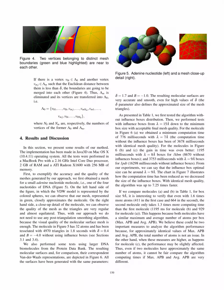
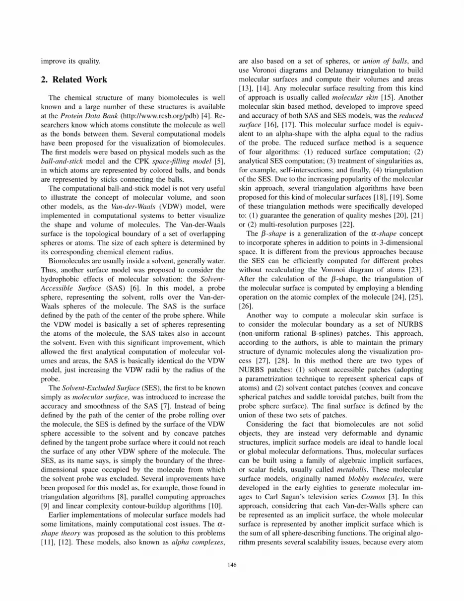
Figure 4. Two vertices belonging to distinct meshboundaries (green and blue highlighted) are near toeach other.

If there is a vertex v0i ∈ Λ0 and another vertexvm j ∈Λm such that the Euclidean distance betweenthem is less than δ , the boundaries are going to bemerged into each other (Figure 4). Thus, Λm iseliminated and its vertices are transferred into Λ0,i.e.

Λ0 = {v01, . . . ,v0i,vm j, . . . ,vmNm ,vm1, . . . ,

vm j,v0i, . . . ,v0N0},

where N0 and Nm are, respectively, the numbers ofvertices of the former Λ0 and Λm.

4. Results and Discussion

In this section, we present some results of our method.The implementation has been made in Java3D on Mac OS X(10.4.11) operating system. All the tests were performed ina MacBook Pro with a 2.16 GHz Intel Core Duo processor,2 GB of RAM and a ATI Radeon X1600 with 256 MB ofmemory.

First, to exemplify the accuracy and the quality of themeshes generated by our approach, we first obtained a meshfor a small adenine nucleotide molecule, i.e., one of the fournucleotides of DNA (Figure 5). On the left hand side ofthe figure, in which the VDW model is represented by thecolored spheres, we can observe that our mesh, representedin green, closely approximates the molecule. On the righthand side, a close-up detail of the molecule, we can observethe quality of the mesh as the triangles are very regularand almost equilateral. Thus, with our approach we donot need to use any post-triangulation smoothing algorithm,because the visual quality of the molecular surface mesh isenough. The molecule in Figure 5 has 32 atoms and has beentesselated with 4970 triangles in 1.8 seconds with δ = 0.4and B = −4.0 without using influence boxes (see Sections3.1 and 3.4).

We also performed some tests using larger DNAbiomolecules from the Protein Data Bank. The resultingmolecular surfaces and, for comparison, their correspondentVan-der-Waals representations, are depicted in Figure 6. Allthe surfaces have been generated with the same parameters:

Figure 5. Adenine nucleotide (left) and a mesh close-updetail (right).

δ = 1.7 and B =−1.0. The resulting molecular surfaces arevery accurate and smooth, even for high values of δ (theδ parameter also defines the approximated size of the meshtriangles).

As presented in Table 1, we first tested the algorithm with-out influence boxes distribution. Then, we performed testswith influence boxes from λ = 15A down to the minimumbox size with acceptable final mesh quality. For the moleculein Figure 6 (a) we obtained a minimum computation timeof 776 milliseconds with λ = 7A (the computation timewithout the influence boxes has been of 3678 millisecondswith identical mesh quality). For the molecules in Figure6 (b) and (c) the gain in time was even better: 1195milliseconds with λ = 8A boxes for 1kbm (8670 withoutinfluences boxes); and 3753 milliseconds with λ = 9A boxesfor 1pdt (16298 milliseconds without influence boxes). Fromour experiments, we can say that the influence box optimalsize can be around λ = 9A. The chart in Figure 7 illustrateshow the computation time has been reduced as we decreasedthe size of the influence boxes. With identical mesh quality,the algorithm was up to 7.25 times faster.

If we compare molecules (a) and (b) in Table 1, for boxsize 9A, it is interesting to verify that even with 1.6 timesmore atoms (411 in the first case and 664 in the second), thesecond molecule only takes 1.3 times more computing timethan the first molecule (1195 ms for molecule (b) and 929for molecule (a)). This happens because both molecules havea similar maximum and average number of atoms per box(Max. APB and Avg. APB). We believe these could be twoimportant measures to analyze the algorithm performancebecause, for approximately identical values of Max. APBand Avg. APB, the total number of atoms is not an issue. Inthe other hand, when these measures are higher, as happensfor molecule (c), the performance may be slightly affected.Thus, even if two molecules have approximately the samenumber of atoms, it cannot be fair compare the algorithmcomputing times if Max. APB and Avg. APB are verydifferent.

150

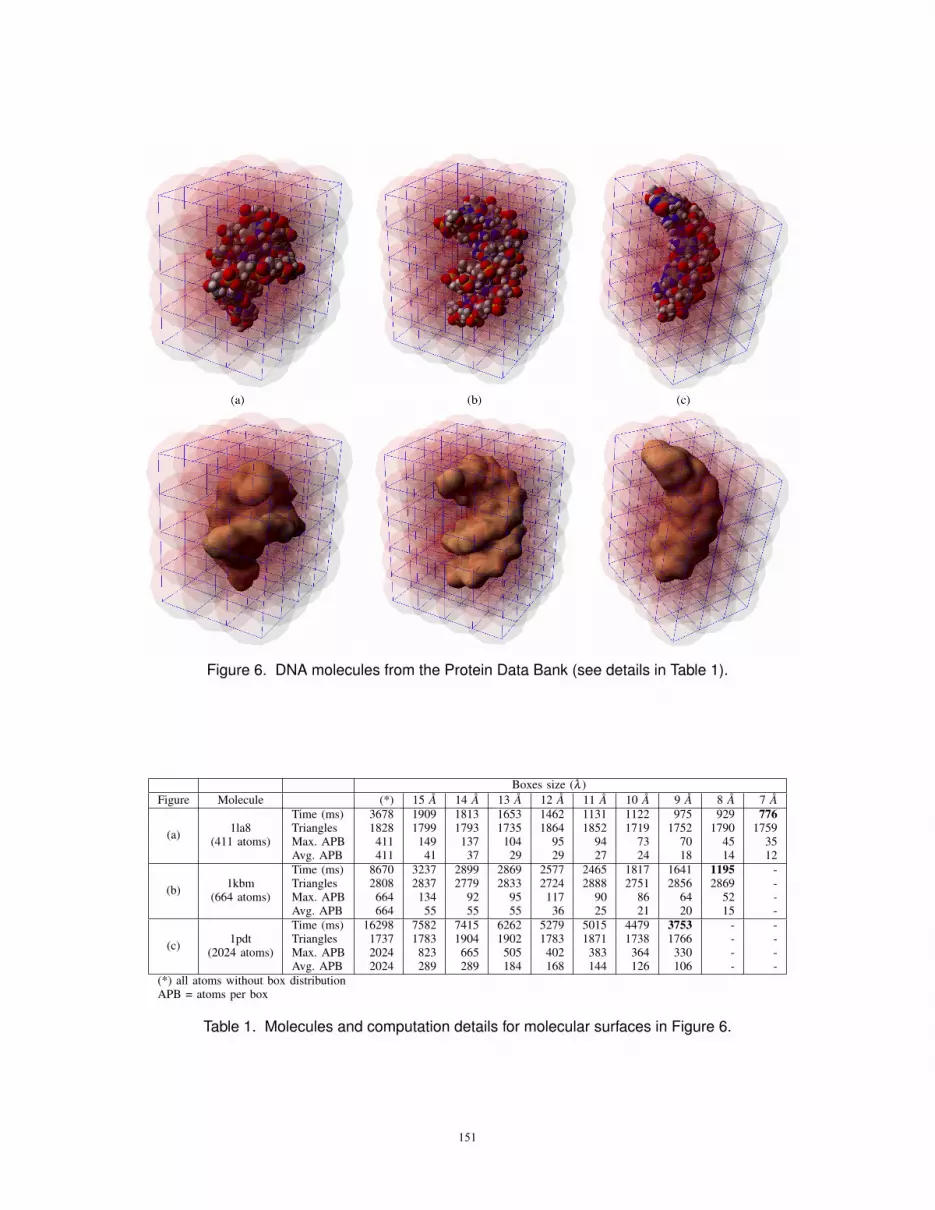
Figure 6. DNA molecules from the Protein Data Bank (see details in Table 1).

Boxes size (λ )Figure Molecule (*) 15 A 14 A 13 A 12 A 11 A 10 A 9 A 8 A 7 A

(a)

Time (ms) 3678 1909 1813 1653 1462 1131 1122 975 929 7761la8 Triangles 1828 1799 1793 1735 1864 1852 1719 1752 1790 1759

(411 atoms) Max. APB 411 149 137 104 95 94 73 70 45 35Avg. APB 411 41 37 29 29 27 24 18 14 12

(b)

Time (ms) 8670 3237 2899 2869 2577 2465 1817 1641 1195 -1kbm Triangles 2808 2837 2779 2833 2724 2888 2751 2856 2869 -

(664 atoms) Max. APB 664 134 92 95 117 90 86 64 52 -Avg. APB 664 55 55 55 36 25 21 20 15 -

(c)

Time (ms) 16298 7582 7415 6262 5279 5015 4479 3753 - -1pdt Triangles 1737 1783 1904 1902 1783 1871 1738 1766 - -

(2024 atoms) Max. APB 2024 823 665 505 402 383 364 330 - -Avg. APB 2024 289 289 184 168 144 126 106 - -

(*) all atoms without box distributionAPB = atoms per box

Table 1. Molecules and computation details for molecular surfaces in Figure 6.

151

Figure 7. Computation times for molecules in Figure 6:(a) 1la8 in blue; (b) 1kbm in red; and (c) 1pdt in green.X-axis represents the size of the influence boxes (* -all atoms without influence box distribution) and Y-axisrepresents the triangulation time in milliseconds. SeeTable 1 for details.

5. Conclusions

In this paper, we propose a numerical continuation algo-rithm for the triangulation of molecular surfaces defined byan isosurface, also known as blobby molecules. The use ofimplicit surfaces is an advantage for dynamic biomolecularapplications with local or global deformability needs. Beinga mesh continuation algorithm it is computationally lessexpensive when compared to space-partitioning approaches.Besides, because the surface sampling is performed using thethree-dimensional Newton’s method, it uses a 1-point itera-tion function instead the usual 2-points functions. Anotheradvantage of this method is the smoothness of the meshes,because the tessellation of molecular surfaces using regularhexagons generates meshes with nearly regular triangles. Weconsider that the overall results, in terms of accuracy andsmoothness, are very good. Finally, we use influence boxesas an efficient way to highly reduce the computation time forlarger for blobby molecules. Using these influence boxes, themolecule’s global density field function takes into accountonly the atoms in a pre-defined neighborhood instead ofconsidering the entire set of atoms in each iteration.

References

[1] H. J. Wolters, “Geometric modeling applications in rationaldrug design: a survey.” Computer Aided Geometric Design,vol. 23, no. 6, pp. 482–494, 2006.

[2] A. Bondi, “Van der Waals Volumes and Radii.” J Phys Chem,vol. 68, no. 3, pp. 441–451, 1964.

[3] J. F. Blinn, “A generalization of algebraic surface drawing,” inSIGGRAPH ’82: Proceedings of the 9th Annual Conferenceon Computer Graphics and Interactive Techniques. NewYork, NY, USA: ACM, 1982, p. 273.

[4] H. M. Berman, J. D. Westbrook, Z. Feng, G. Gilliland, T. N.Bhat, H. Weissig, I. N. Shindyalov, and P. E. Bourne, “TheProtein Data Bank,” Nucleic Acids Research, vol. 28, no. 1,pp. 235–242, 2000.

[5] R. B. Corey and L. Pauling, “Molecular Models of AminoAcids, Peptides, and Proteins,” Review of Scientific Instru-ments, vol. 24, no. 8, pp. 621–627, 1953.

[6] B. Lee and F. Richards, “The interpretation of protein struc-tures: estimation of static accessibility,” J. Mol. Biol., vol. 55,pp. 379–400, Feb 1971.

[7] M. L. Connolly, “Solvent-accessible surfaces of proteins andnucleic acids.” Science, vol. 221, no. 4612, pp. 709–13, 1983.

[8] ——, “Molecular surface triangulation.” Journal of AppliedCrystallography, vol. 18, pp. 499–503, 1985.

[9] A. Varshney and F. P. Brooks, “Fast analytical computationof Richards’s smooth molecular surface,” in VIS ’93: Pro-ceedings of the 4th Conference on Visualization ’93, 1993,pp. 300–307.

[10] M. Totrov and R. Abagyan, “The contour-buildup algorithmto calculate the analytical molecular surface,” J. Struct. Biol.,vol. 116, pp. 138–143, 1996.

[11] N. Akkiraju, H. Edelsbrunner, P. Fu, and J. Qian, “Viewinggeometric protein structures from inside a cave,” IEEE Com-put. Graph. Appl., vol. 16, no. 4, pp. 58–61, 1996.

[12] H. Edelsbrunner, M. Facello, and J. Liang, “On the definitionand the construction of pockets in macromolecules,” DiscreteAppl. Math., vol. 88, no. 1-3, pp. 83–102, 1998.

[13] H. Edelsbrunner, “The union of balls and its dual shape,”in SCG ’93: Proceedings of the Ninth Annual Symposiumon Computational Geometry. New York, NY, USA: ACM,1993, pp. 218–231.

[14] H. Edelsbrunner and E. P. Mucke, “Three-dimensional alphashapes,” ACM Trans. Graph., vol. 13, no. 1, pp. 43–72, 1994.

[15] H. Edelsbrunner and P. Koehl, “The geometry of biomolecu-lar solvation,” Combinatorial and Computational Geometry,vol. 52, pp. 243–275, 2005.

[16] M. F. Sanner, A. J. Olson, and J.-C. Spehner, “Fast and robustcomputation of molecular surfaces,” in SCG ’95: Proceedingsof the Eleventh Annual Symposium on Computational Geom-etry. New York, NY, USA: ACM, 1995, pp. 406–407.

[17] M. Sanner, A. Olson, and J. Spehner, “Reduced surface: anefficient way to compute molecular surfaces,” Biopolymers,vol. 38, pp. 305–320, Mar 1996.

[18] N. Akkiraju and H. Edelsbrunner, “Triangulating the surfaceof a molecule,” Discrete Appl. Math., vol. 71, no. 1-3, pp.5–22, 1996.

[19] H.-L. Cheng, T. K. Dey, H. Edelsbrunner, and J. Sullivan,“Dynamic skin triangulation,” in SODA ’01: Proceedingsof the Twelfth Annual ACM-SIAM Symposium on DiscreteAlgorithms. Philadelphia, PA, USA: Society for Industrialand Applied Mathematics, 2001, pp. 47–56.

152

[20] H.-L. Cheng and X. Shi, “Guaranteed Quality Triangulationof Molecular Skin Surfaces,” VIS, vol. 00, pp. 481–488, 2004.

[21] ——, “Quality mesh generation for molecular skin surfacesusing restricted union of balls,” VIS, vol. 00, p. 51, 2005.

[22] C. Bajaj, V. Pascucci, A. Shamir, R. Holt, and A. Netravali,“Multiresolution molecular shapes. Technical Report 99-42,TICAM, University of Texas at Austin.” 1999.

[23] J. Ryu, R. Park, and D.-S. Kim, “Connolly Surface on anAtomic Structure via Voronoi Diagram of Atoms,” J. Comput.Sci. Technol., vol. 21, no. 2, pp. 255–260, 2006.

[24] J. Ryu, R. Park, J. Seo, C. Kim, H. Lee, and D.-S. Kim,“Real-time triangulation of molecular surfaces,” in ICCSA (1).Berlin / Heidelberg: Springer, 2007, pp. 55–67.

[25] J. Ryu, R. Park, and D.-S. Kim, “Molecular surfaces onproteins via beta shapes,” Comput. Aided Des., vol. 39, no. 12,pp. 1042–1057, 2007.

[26] J. Ryu, Y. Cho, and D.-S. Kim, “Triangulation ofmolecular surfaces,” Computer-Aided Design, vol. InPress, Corrected Proof, pp. –, 2009. [Online]. Avail-able: http://www.sciencedirect.com/science/article/B6TYR-4VT0X6Y-1/2/cc3daabeab9178d81ad8c8e613d6b6d0

[27] C. Bajaj, H. Y. Lee, R. Merkert, and V. Pascucci, “NURBSbased B-rep models for macromolecules and their properties,”in SMA ’97: Proceedings of the Fourth ACM Symposium onSolid Modeling and Applications. New York, NY, USA:ACM, 1997, pp. 217–228.

[28] C. L. Bajaj, V. Pascucci, A. Shamir, R. J. Holt, and A. N. Ne-travali, “Dynamic maintenance and visualization of molecularsurfaces,” Discrete Appl. Math., vol. 127, no. 1, pp. 23–51,2003.

[29] G. Wyvill, C. McPheeters, and B. Wyvill, “Soft objects,” inProceedings of Computer Graphics Tokyo ’86 on AdvancedComputer Graphics. New York, NY, USA: Springer-VerlagNew York, Inc., 1986, pp. 113–128.

[30] ——, “Data structure for soft objects,” The Visual Computer,vol. 2, no. 4, pp. 227–234, 1986.

[31] Y. Zhang, G. Xu, and C. Bajaj, “Quality meshing of implicitsolvation models of biomolecular structures,” Comput. AidedGeom. Des., vol. 23, no. 6, pp. 510–530, 2006.

[32] W. E. Lorensen and H. E. Cline, “Marching cubes: A highresolution 3d surface construction algorithm,” SIGGRAPHComput. Graph., vol. 21, no. 4, pp. 163–169, 1987.

[33] E. Hartmann, “A marching method for the triangulation ofsurfaces,” The Visual Computer, vol. 14, no. 3, pp. 95–108,1998.

[34] A. N. Raposo and A. J. P. Gomes, “Polygonization ofmulti-component non-manifold implicit surfaces through asymbolic-numerical continuation algorithm,” in GRAPHITE’06: Proceedings of the 4th International Conference onComputer Graphics and Interactive Techniques in Australasiaand Southeast Asia. New York, NY, USA: ACM, 2006, pp.399–406.

[35] J. Bloomenthal, “Polygonization of implicit surfaces,” Com-put. Aided Geom. Des., vol. 5, no. 4, pp. 341–355, 1988.

153