Tutorial of numerical continuation and bifurcation theory forsystems and synthetic biology

Mark Blyth1, Ludovic Renson ∗2, and Lucia Marucci ∗1,3,4

1Department of Engineering Mathematics, University of Bristol, Bristol BS8 1UB, UK.2Department of Mechanical Engineering, Imperial College London, South Kensington

Campus, London SW7 2AZ, UK3School of Cellular and Molecular Medicine, University of Bristol, Bristol BS8 1TD, UK.

4BrisSynBio, Bristol BS8 1TQ, UK

Abstract

Mathematical modelling allows us to concisely describe fundamental principles in biology. Anal-ysis of models can help to both explain known phenomena, and predict the existence of new, unseenbehaviours. Model analysis is often a complex task, such that we have little choice but to approachthe problem with computational methods. Numerical continuation is a computational method foranalysing the dynamics of nonlinear models by algorithmically detecting bifurcations. Here we aimto promote the use of numerical continuation tools by providing an introduction to nonlinear dy-namics and numerical bifurcation analysis. Many numerical continuation packages are available,covering a wide range of system classes; a review of these packages is provided, to help both new andexperienced practitioners in choosing the appropriate software tools for their needs.

1 IntroductionComputational biology uses mathematical tools to understand the mechanisms that orchestrate life andliving processes [1]. Differential equations are a powerful tool for describing how biological processesbehave, based on the values and rate of change of a set of variables. Both the equations and theirsolutions can be analysed to explain observed phenomena, and predict novel and unseen behaviours.

A differential equation is linear only if its rates of change follow simple proportional relationships.Biological systems are rarely linear, and instead fall into the wide category of nonlinear systems [2].Nonlinearity arises from complex interplays between the constituent components of a system, such as thesubtle mutual dependencies of a neuron’s ionic currents [3], or the complex feedback loops of mammalianerythropoiesis [4]. Nonlinearity allows for a rich set of non-trivial behaviours, at the expense of simplicity.Nonlinear systems are rarely analytically tractable – it is not generally possible to obtain a closed-formsolution to a nonlinear differential equation. As a result, the field of nonlinear dynamics considers howbest to analyse the equations without actually solving them.

The challenges in working with nonlinear systems are justified by their immense explanatory power.Classic examples include the work of Hodgkin and Huxley [5], which laid the foundations of modern neu-roscience; the Mackey-Glass equation [6], which describes the nuanced effects of time-delayed feedbackon respiratory and hematopoietic diseases; and the Lotka-Volterra model [7], which describes the inter-actions between populations of predators and prey. Synthetic biology makes extensive use of nonlinearmodels and their associated analysis tools, to design and represent artificially engineered gene networks[8, 9].

Numerical continuation is a standard method within the nonlinear dynamics community. In thiscontext, it is used to computationally analyse nonlinear differential equations. Here we aim to introducethe method to those without a background in nonlinear dynamics. Examples are provided to highlightexisting biological applications, and to demonstrate the applicability of nonlinear dynamics to biology.Section 2 introduces some key ideas from nonlinear dynamics. Section 3 discusses a nonlinear model,which is then used in a numerical continuation experiment in section 4. This tutorial helps to motivate

∗Co-last and co-corresponding authors: l.renson@imperial.ac.uk; lucia.marucci@bristol.ac.uk

1

arX

iv:2

008.

0522

6v1

[q-

bio.

QM

] 1

2 A

ug 2

020

some of the core ideas from the field. A wide range of software packages are available for numericalcontinuation, which are reviewed in section 5. Note that while some existing publications include a surveyof these tools (see [10, 11]) they focus primarily on the history and design approaches of the software;we instead consider the various practicalities and usage cases, to help users choose the appropriate toolfor their needs.

2 Nonlinear dynamicsHere we introduce some foundational ideas from nonlinear dynamics, and motivate the concept of a bifur-cation. These ideas are then demonstrated in practice in section 4. See [12, 13, 14] for a comprehensivediscussion of bifurcations and nonlinear dynamics, and [2, 3, 15] for an introduction from a mathematicalbiology perspective. The authors particularly recommend [12] for a very readable entry-point to the field.

Differential equations describe how the state of a system changes with respect to an independentvariable. Time is often taken as the independent variable, in which case the differential equationsdescribe the temporal evolution of states. A system state quantifies all necessary information requiredto describe and predict the behaviours of interest. For some classes of differential equation, states mustbe functions, such as the population density of a species in a partial differential equation model ofpredator-prey interaction, or the previous values of red blood cell counts in a delay differential equationfor erythropoiesis; see [16] for a wide variety of examples. Such classes of differential equation are notconsidered here. Instead, the proceeding work considers ordinary differential equations, where a set ofdependent variables evolves under a single time-like dependent variable, with the evolution dependingonly on the current value of the state.

The qualitative behaviour of a system is referred to as its dynamics. For example, the dynamicscould be quiescent if the system remains settled at a steady-state, or oscillatory if the state fluctuatesin a consistent, repetitive manner, or chaotic if the state changes deterministically but unpredictably.A system can settle to different dynamics from different initial states, for example when quiescent andoscillatory behaviours coexist.

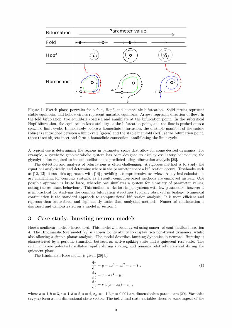
System dynamics generally depend a set of external parameters. The parameter dependence is oftennon-trivial, such that changing a parameter value by just a small amount can sometimes lead to drasticchanges in the system behaviours. An extreme example of this can be seen in the canard explosion of afood-chain model [17]. Here, the population size transitions between steady and rapidly oscillating in anexponentially small region of parameter space. When a change the parameter value causes a qualitativechange in dynamics, a bifurcation is said to have occurred. A bifurcation occurs at a parameter value ifa system contains dynamics within a neighbourhood of the parameter that differ from the dynamics atthe parameter. That is, no matter how small a distance we move away from the bifurcation point, wecan always find system behaviours that are qualitatively different to those that occur at the bifurcationpoint. A bifurcation diagram shows how invariant sets (such as steady-state position) or measures onthe system (such as oscillation amplitude) change, as a parameter is varied. The simplest bifurcationsinclude the fold, Hopf, and homoclinic bifurcations, as sketched in figure 1. These can be observed whenonly a single parameter is varied.

A fold bifurcation occurs when a stable and unstable equilibrium annihilate. Pairs of fold bifurcationsoften lead to switch-like behaviours in biological systems [18]. This happens when a region of bistabilityoccurs, where two stable equilibria coexist. The switching behaviour arises when an external stimuluspushes the system from one equilibrium to the other. Fold-induced multistability can model a widerange of behaviours, including metabolic pathway dynamics [19], visual perception tasks [20], manybiological feedback systems [21], and cell specialisation, whereby cells specialise by losing unspecialisedstates through fold bifurcations [22, 23]. Bistable dynamics are regularly exploited in synthetic biology,to design and predict system dynamics [24]. For example, saddle-node bifurcations in eukaryotic cellsignalling pathways leads to bistability [25], which has been used to create a cellular hysteresis-looposcillator [26].

A homoclinic bifurcation happens when a limit cycle approaches, collides with, and is annihilatedby a saddle equilibrium. This is sketched, in the case of a stable limit cycle, in figure 1. Homoclinicbifurcations are a key cause of spike termination in neurons [3].

Hopf bifurcations are the simplest way for a system to transition to oscillatory behaviour. In aHopf bifurcation, an equilibrium changes stability and a limit cycle appears or disappears around it, assketched in figure 1. This can occur, for example, in a predator-prey system – the system undergoesa Hopf bifurcation when feedbacks between the competing populations cause oscillations to emerge inthe population sizes [27]. Hopf bifurcations can be used when designing synthetic biological systems.

2

Bifurcation Parameter value

Fold

Hopf

Homoclinic

Figure 1: Sketch phase portraits for a fold, Hopf, and homoclinic bifurcation. Solid circles representstable equilibria, and hollow circles represent unstable equilibria. Arrows represent direction of flow. Inthe fold bifurcation, two equilibria coalesce and annihilate at the bifurcation point. In the subcriticalHopf bifurcation, the equilibrium loses stability at the bifurcation point, and the flow is pushed onto aspawned limit cycle. Immediately before a homoclinic bifurcation, the unstable manifold of the saddle(blue) is sandwiched between a limit cycle (green) and the stable manifold (red); at the bifurcation point,these three objects meet and form a homoclinic connection, annihilating the limit cycle.

A typical use is determining the regions in parameter space that allow for some desired dynamics. Forexample, a synthetic gene-metabolic system has been designed to display oscillatory behaviours; theglycolytic flux required to induce oscillations is predicted using bifurcation analysis [28].

The detection and analysis of bifurcations is often challenging. A rigorous method is to study theequations analytically, and determine where in the parameter space a bifurcation occurs. Textbooks suchas [12, 13] discuss this approach, with [14] providing a comprehensive overview. Analytical calculationsare challenging for complex systems; as a result, computer-based methods are employed instead. Onepossible approach is brute force, whereby one simulates a system for a variety of parameter values,noting the resultant behaviours. This method works for simple systems with few parameters, however itis impractical for studying the complex bifurcation structures typically observed in biology. Numericalcontinuation is the standard approach to computational bifurcation analysis. It is more efficient andrigorous than brute force, and significantly easier than analytical methods. Numerical continuation isdiscussed and demonstrated on a model in section 4.

3 Case study: bursting neuron modelsHere a nonlinear model is introduced. This model will be analysed using numerical continuation in section4. The Hindmarsh-Rose model [29] is chosen for its ability to display rich non-trivial dynamics, whilstalso allowing a simple planar analysis. The model describes bursting dynamics in neurons. Bursting ischaracterised by a periodic transition between an active spiking state and a quiescent rest state. Thecell membrane potential oscillates rapidly during spiking, and remains relatively constant during thequiescent phase.

The Hindmarsh-Rose model is given [29] by

dx

dt= y − ax3 + bx2 − z + I , (1)

dy

dt= c− dx2 − y ,

dz

dt= r [s(x− xR)− z] ,

where a = 1, b = 3, c = 1, d = 5, s = 4, xR = −1.6, r = 0.001 are dimensionless parameters [29]. Variables(x, y, z) form a non-dimensional state vector. The individual state variables describe some aspect of the

3

system that we are interested in learning about: x models the membrane potential of a bursting cell,y the main currents into and out of the cell, and z an adaptive (calcium-like) current. The parametersdescribe the set of controllable and uncontrollable inputs to the system. For example, parameter I modelsan externally applied current, and is easily controllable by an experimenter; conversely, r measures thetimescale separation of the adaptive current, which is less trivial to modify experimentally.

The magnitude of the z-variable’s time-derivative is approximately r times smaller than that of the xand y variables. The x, y variables thus change much more rapidly than z, and are said to form the ‘fastsubsystem’; z, changing slowly, forms the slow subsystem. Consider the singular limit r → 0; the slowsubsystem ceases to change and z becomes constant, fixed at its initial condition z(0). Our investigativeprocedure, as pioneered by Rinzel [30], exploits this as follows. The slow variable z is treated as aparameter of the fast subsystem; the dependence of the fast-subsystem dynamics on z is investigatedwith numerical continuation; the slow subsystem is then reintroducted, revealling the cause of burstingdynamics.

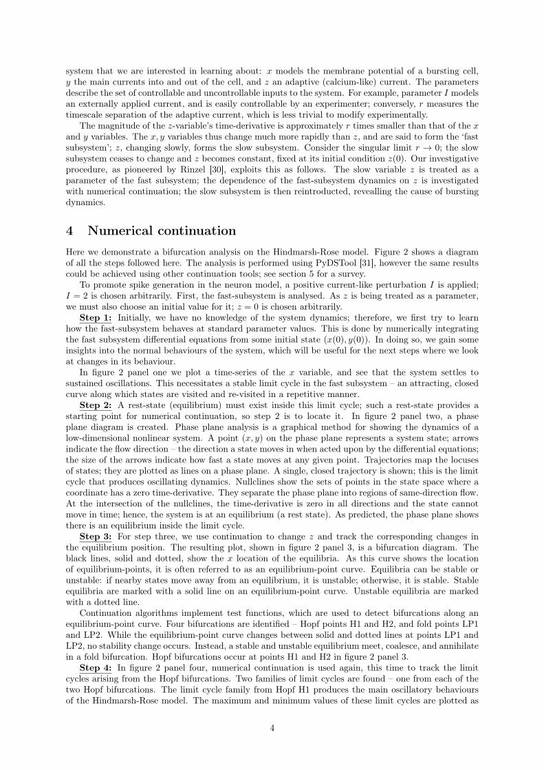
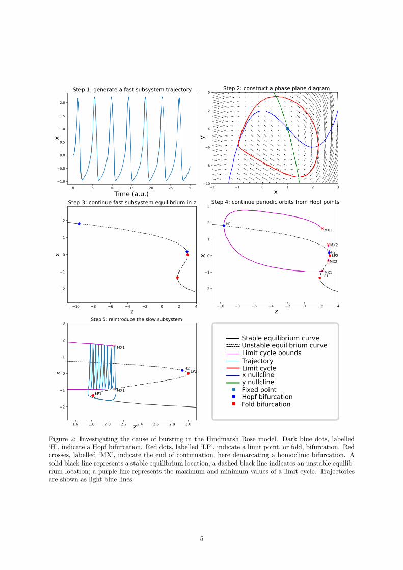
4 Numerical continuationHere we demonstrate a bifurcation analysis on the Hindmarsh-Rose model. Figure 2 shows a diagramof all the steps followed here. The analysis is performed using PyDSTool [31], however the same resultscould be achieved using other continuation tools; see section 5 for a survey.

To promote spike generation in the neuron model, a positive current-like perturbation I is applied;I = 2 is chosen arbitrarily. First, the fast-subsystem is analysed. As z is being treated as a parameter,we must also choose an initial value for it; z = 0 is chosen arbitrarily.

Step 1: Initially, we have no knowledge of the system dynamics; therefore, we first try to learnhow the fast-subsystem behaves at standard parameter values. This is done by numerically integratingthe fast subsystem differential equations from some initial state (x(0), y(0)). In doing so, we gain someinsights into the normal behaviours of the system, which will be useful for the next steps where we lookat changes in its behaviour.

In figure 2 panel one we plot a time-series of the x variable, and see that the system settles tosustained oscillations. This necessitates a stable limit cycle in the fast subsystem – an attracting, closedcurve along which states are visited and re-visited in a repetitive manner.

Step 2: A rest-state (equilibrium) must exist inside this limit cycle; such a rest-state provides astarting point for numerical continuation, so step 2 is to locate it. In figure 2 panel two, a phaseplane diagram is created. Phase plane analysis is a graphical method for showing the dynamics of alow-dimensional nonlinear system. A point (x, y) on the phase plane represents a system state; arrowsindicate the flow direction – the direction a state moves in when acted upon by the differential equations;the size of the arrows indicate how fast a state moves at any given point. Trajectories map the locusesof states; they are plotted as lines on a phase plane. A single, closed trajectory is shown; this is the limitcycle that produces oscillating dynamics. Nullclines show the sets of points in the state space where acoordinate has a zero time-derivative. They separate the phase plane into regions of same-direction flow.At the intersection of the nullclines, the time-derivative is zero in all directions and the state cannotmove in time; hence, the system is at an equilibrium (a rest state). As predicted, the phase plane showsthere is an equilibrium inside the limit cycle.

Step 3: For step three, we use continuation to change z and track the corresponding changes inthe equilibrium position. The resulting plot, shown in figure 2 panel 3, is a bifurcation diagram. Theblack lines, solid and dotted, show the x location of the equilibria. As this curve shows the locationof equilibrium-points, it is often referred to as an equilibrium-point curve. Equilibria can be stable orunstable: if nearby states move away from an equilibrium, it is unstable; otherwise, it is stable. Stableequilibria are marked with a solid line on an equilibrium-point curve. Unstable equilibria are markedwith a dotted line.

Continuation algorithms implement test functions, which are used to detect bifurcations along anequilibrium-point curve. Four bifurcations are identified – Hopf points H1 and H2, and fold points LP1and LP2. While the equilibrium-point curve changes between solid and dotted lines at points LP1 andLP2, no stability change occurs. Instead, a stable and unstable equilibrium meet, coalesce, and annihilatein a fold bifurcation. Hopf bifurcations occur at points H1 and H2 in figure 2 panel 3.

Step 4: In figure 2 panel four, numerical continuation is used again, this time to track the limitcycles arising from the Hopf bifurcations. Two families of limit cycles are found – one from each of thetwo Hopf bifurcations. The limit cycle family from Hopf H1 produces the main oscillatory behavioursof the Hindmarsh-Rose model. The maximum and minimum values of these limit cycles are plotted as

4

Time (a.u.)

x

x

z

y

x

x

z

x x nullcliney nullclineFixed point

Limit cycle

Fold bifurcationHopf bifurcation

Stable equilibrium curve

TrajectoryLimit cycle boundsUnstable equilibrium curve

z

Figure 2: Investigating the cause of bursting in the Hindmarsh Rose model. Dark blue dots, labelled‘H’, indicate a Hopf bifurcation. Red dots, labelled ‘LP’, indicate a limit point, or fold, bifurcation. Redcrosses, labelled ‘MX’, indicate the end of continuation, here demarcating a homoclinic bifurcation. Asolid black line represents a stable equilibrium location; a dashed black line indicates an unstable equilib-rium location; a purple line represents the maximum and minimum values of a limit cycle. Trajectoriesare shown as light blue lines.

5

purple lines on the bifurcation diagram. Homoclinic bifurcations are observed at points MX1 and MX2in figure 2. Note that MX does not mean a homoclinic bifurcation has been detected, but that thecontinuation algorithm failed to converge. It is up to the user to identify that the convergence failure isdue to the limit cycles disappearing in a homoclinic bifucation.

Step 5: In figure 2 panel five, we reintroduce the slow subsystem to uncover the cause of bursting.A trajectory of the full system is computed and plotted in the (z, x) plane, on top of the bifurcationdiagram. Bursting behaviour is seen to arise as follows. Bistability exists between an equilibrium anda limit cycle. This bistable region starts at a fold bifurcation on the left, and ends at a homoclinicbifurcation on the right, respectively labelled LP1 and MX1 in figure 2. The slow subsystem periodicallydrives the fast subsystem across this pair of bifurcations. The state sits at an equilibrium until itdisappears though fold bifurcation LP1. This causes the system to jump onto the limit cycle originatingat Hopf H1, with the limit cycle producing spiking dynamics. Now z flows in the opposite direction,until the limit cycle disappears through homoclinic bifurcation MX1. The system jumps back to theequilibrium, and spiking is terminated. Once again the flow of z changes direction, and the patternrepeats. This periodic transition between an equilibrium and limit cycle causes a transition betweenquiescent and spiking states resepectively, and hence bursting behaviours arise. The use of numericalcontinuation allows us to find the points at which these bifurcations occur, and to generate diagramswhich graphically explain the behaviour. With experience, these diagrams become an invaluable tool tounderstanding the dynamics of nonlinear systems.

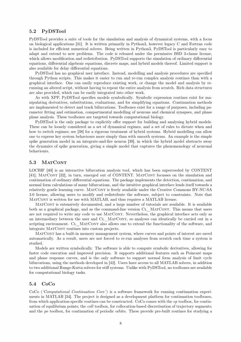
5 Review of continuation softwareNumerous software packages have been written for performing numerical continuation. Here, MatCont[32], PyDSTool [31], XPPAUTO [33], and CoCo [34] – the four most common continuation tools – arediscussed. These are all applicable to ordinary differential equations. Tools for other system classes aresurveyed in section 5.5.

Tables 1 and 2 provide a comparison of key features of the main continuation software tools. Table1 shows a summary of the general software features; table 2 shows which of various bifurcations eachsoftware tool is able to detect, and which it is able to continue. Each tool has its own best-usage criteria.For example, MatCont is able to detect and continue the most bifurcations of the tools, however it canonly simulate ordinary differential equations. XPPAUTO can simulate a wider range of system types,at the expense of detecting fewer bifurcation. CoCo is a development toolbox, so can be applied toany continuation problem. PyDSTool and XPPAUTO both use low-level integrators and continuationalgorithms, making them significantly faster than CoCo and MatCont. The choice of tool thereforecomes down to user preferences such as coding language and interface type, and performance factors suchas speed and capabilities. Note that some bifurcations which are not detected by a software tool canstill be identified by users. For example, XPPAUTO cannot explicitly detect cusp bifurcations, howeverthey are easily spotted from the intersection of two fold manifolds.

5.1 XPPAUTOXPPAUTO (also called XPPAUT, XPP) is a combined simulation and analysis package [33]. It providesan interface to AUTO [35, 36, 37] for numerical continuation. XPPAUTO is one of the oldest dynamicalsystems tools to still see regular use. A large community and a range of resources are available, see forexample [33]. Nevertheless, the age of the software also lends itself to a somewhat dated user interface.The program sometimes crashes; as no scripting interface is available, it can be difficult to restart theanalysis from the point where it was interrupted.

XPPAUTO is used through a graphical interface. Models are specified symbolically in text files,meaning no knowledge of coding is required. Most features of AUTO are accessible, allowing users toexploit its powerful continuation routines without writing Fortran code. XPP is capable of simulatingmany system classes, including ordinary, delay, and stochastic differential equations, boundary valueproblems, and difference and functional equations. The package is written in C, and source code isreleased under the GNU GPL v2 license, allowing modification and redistribution. Nevertheless, beinga compiled GUI package, the code base does not easily lend itself towards being extended or adapted tonovel problems.

XPPAUTO has a wide range of features: over a dozen solvers are available, covering forward andbackward integration for a range of stiff and non-stiff classes of system. Tools are also provided for phaseplane analysis, and methods exist to create Poincaré sections and animations.

6

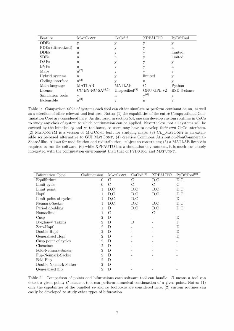
Feature MatCont CoCo(1) XPPAUTO PyDSToolODEs y y y yPDEs (discretized) n y y nDDEs n y y limitedSDEs n n y limitedDAEs n y y yBVPs n y y nMaps n(2) y y yHybrid systems n y limited yCoding interface n(3) y n yMain language MATLAB MATLAB C PythonLicense CC BY-NC-SA(4,5) Unspecified(5) GNU GPL v2 BSD 3-clauseSimulation tools y n y(6) yExtensible n(3) y n y

Table 1: Comparison table of systems each tool can either simulate or perform continuation on, as wellas a selection of other relevant tool features. Notes: (1) the capabilities of the entire Computational Con-tinuation Core are considered here. As discussed in section 5.4, one can develop custom routines in CoCoto study any class of system to which continuation can be applied. Nevertheless, not all systems will becovered by the bundled ep and po toolboxes, so users may have to develop their own CoCo interfaces.(2) MatContM is a version of MatCont built for studying maps; (3) Cl_MatCont is an exten-sible script-based alternative to GUI MatCont; (4) creative Commons Attribution-NonCommercial-ShareAlike. Allows for modification and redistribution, subject to constraints; (5) a MATLAB license isrequired to run the software; (6) while XPPAUTO has a simulation environment, it is much less closelyintegrated with the continuation environment than that of PyDSTool and MatCont.

Bifurcation Type Codimension MatCont CoCo(1,2) XPPAUTO PyDSTool(2)

Equilibrium 0 C C D,C D,CLimit cycle 0 C C C CLimit point 1 D,C D,C D,C D,CHopf 1 D,C D,C D,C D,CLimit point of cycles 1 D,C D,C - DNeimark-Sacker 1 D,C D,C D,C D,CPeriod doubling 1 D D,C D,C D,CHomoclinic 1 C - C -Cusp 2 D - - DBogdanov Takens 2 D D - DZero-Hopf 2 D - - DDouble Hopf 2 D - - DGeneralised Hopf 2 D - - DCusp point of cycles 2 D - - -Chenciner 2 D - - -Fold-Neimark-Sacker 2 D - - -Flip-Neimark-Sacker 2 D - - -Fold-Flip 2 D - - -Double Niemark-Sacker 2 D - - -Generalised flip 2 D - - -

Table 2: Comparison of points and bifurcations each software tool can handle. D means a tool candetect a given point; C means a tool can perform numerical continuation of a given point. Notes: (1)only the capabilities of the bundled ep and po toolboxes are considered here; (2) custom routines caneasily be developed to study other types of bifurcation.

7

5.2 PyDSTool

PyDSTool provides a suite of tools for the simulation and analysis of dynamical systems, with a focuson biological applications [31]. It is written primarily in Python3, however legacy C and Fortran codeis included for efficient numerical solvers. Being written in Python3, PyDSTool is particularly easy toadapt and extend to new problems. The code is released under the permissive BSD 3-clause license,which allows modification and redistribution. PyDSTool supports the simulation of ordinary differentialequations, differential algebraic equations, discrete maps, and hybrid models thereof. Limited support isalso available for delay differential equations.

PyDSTool has no graphical user interface. Instead, modelling and analysis procedures are specifiedthrough Python scripts. This makes it easier to run and re-run complex analysis routines than with agraphical interface. One can easily reproduce existing work, or change the model and analysis by re-running an altered script, without having to repeat the entire analysis from scratch. Rich data structuresare also provided, which can be easily integrated into other work.

As with XPP, PyDSTool specifies models symbolically. Symbolic expression routines exist for ma-nipulating derivatives, substitutions, evaluations, and for simplifying equations. Continuation methodsare implemented to detect and track bifurcations. Toolboxes exist for a range of purposes, including pa-rameter fitting and estimation, compartmental modelling of neurons and chemical synapses, and phaseplane analysis. These toolboxes are targeted towards computational biology.

PyDSTool is the only package to explicitly offer support for building and analysing hybrid models.These can be loosely considered as a set of dynamical regimes, and a set of rules to dictate when andhow to switch regimes; see [38] for a rigorous treatment of hybrid systems. Hybrid modelling can allowone to express key system behaviours more simply than with smooth systems. An example is the simplespike generation model in an integrate-and-fire neuron [39], in which the hybrid model abstracts awaythe dynamics of spike generation, giving a simple model that captures the phenomenology of neuronalbehaviours.

5.3 MatCont

LOCBIF [40] is an interactive bifurcation analysis tool, which has been superceeded by CONTENT[41]; MatCont [32], in turn, emerged out of CONTENT. MatCont focusses on the simulation andcontinuation of ordinary differential equations. The package implements the detection, continuation, andnormal form calculations of many bifurcations, and the intuitive graphical interface lends itself towards arelatively gentle learning curve. MatCont is freely available under the Creative Commons BY-NC-SA3.0 license, allowing users to modify and redistribute the software, subject to constraints. Note thatMatCont is written for use with MATLAB, and thus requires a MATLAB license.

MatCont is extensively documented, and a large number of tutorials are available. It is availableboth as a graphical package, and as the command-line version Cl_MatCont. This means that usersare not required to write any code to use MatCont. Nevertheless, the graphical interface acts only asan intermediary between the user and Cl_MatCont, so analyses can identically be carried out in ascripting environment. Cl_MatCont also allows one to extend the functionality of the software, andintegrate MatCont routines into custom projects.

MatCont has a built-in memory management system, where curves and points of interest are savedautomatically. As a result, users are not forced to re-run analyses from scratch each time a system isstudied.

Models are written symbolically. The software is able to compute symbolic derivatives, allowing forfaster code execution and improved precision. It supports additional features such as Poincaré mapsand phase response curves, and is the only software to support normal form analysis of limit cyclebifurcations, using the methods developed in [42]. Users have access to all MATLAB solvers, in additionto two additional Runge-Kutta solvers for stiff systems. Unlike with PyDSTool, no toolboxes are availablefor computational biology tasks.

5.4 CoCo

CoCo (‘Computational Continuation Core’ ) is a software framework for running continuation experi-ments in MATLAB [34]. The project is designed as a development platform for continuation toolboxes,from which application-specific routines can be constructed. CoCo comes with the ep toolbox, for contin-uation of equilibrium points; the coll toolbox, for collocation-based discretisation of trajectory segments;and the po toolbox, for continuation of periodic orbits. These provide pre-built routines for studying a

8

range of bifurcations. ‘CoCo’ is used here to refer to both the continuation core itself, and these bundledtoolboxes.

Much like PyDSTool, CoCo is entirely scripting-based. Models are specified as MATLAB functions,which are passed through various functions to set up and run a continuation experiment. As withPyDSTool, the scripting design allows one to share the codes used to create any analyses. Analysescan be run, modified, and re-run more easily than for graphical-only tools. Nevertheless, the use of ascripting interface requires practitioners to be sufficiently competent with MATLAB programming.

CoCo has less support for detecting and continuing bifurcations than MatCont and PyDSTool; itscapabilities are similar to those of XPPAUTO. However, CoCo is designed specifically for extensibility –users with knowledge of bifurcation analysis and programming will be able to design codes for handlingarbitrary bifurcations. With sufficient mathematical and coding skills, one can develop methods in CoCoto handle any problem that can be solved using continuation, making it a powerful tool for advancedusers.

CoCo sits within a MATLAB workflow. MATLAB routines can be used to simulate a system, searchfor fixed points, generate phase plane diagrams, etc. The results of these procedures can then be used todetermine how continuation should be applied. This differs from the other tools discussed here, in whichsimulation, analysis and continuation are all available within one single package.

5.5 Other continuation tools

Numerous other continuation packages exist, both for ODEs and other classes of system. These arediscussed here.

The various versions of AUTO [35, 36, 37] can be used for continuation experiments. Note thatPyDSTool [31] and XPPAUTO [33] both provide AUTO interfaces.

DsTool [43] aims to provide an interactive package for all computations regarding dynamical systems.PyDSTool is designed as a modern replacement for DsTool [31]. LINBLF [44] and CANDYS/QA [45]are other tools for the bifurcation analysis of ordinary differential equations.

The introduction of time delays into a system can give rise to complex dynamics. Systems becomeinfinite-dimensional, and must be given initial data over a time interval. Delay differential equationsdescribe a range of phenomena in biology and physiology, in areas such as immunology [46], neuronalinteractions [47], and biochemical reactions [48]; reviews are provided in [49, 50]. Due to the difficultyin analysing delay equations, numerics are regularly used. Two main packages exist for these purposes.DDE BIFTOOL [51] is a scripting-based MATLAB package for analysis of systems with fixed delays.It provides stability analysis and tracking of equilibrium and limit cycle solutions, and is capable oftracking bifurcations. Knut [52] is a graphical package for analysing and simulating DDEs. It supportsstability analysis, orbit continuation and bifurcation detection in one parameter, and has methods for thetwo-parameter continuation of some bifurcations. Unlike DDE BIFTOOL, it requires no programmingknowlege to use; being written in C++, it is also faster.

Partial differential equations describe derivative problems over multiple independent variables. Thisis often used to describe continuum problems in biology [16]. PDEs have been used in developmentalbiology to model self-organisation and the emergence of complex structures in multicellular systems [53],in ecology to model the spatial dynamics of populations [54], and in systems biology to describe theprocess of morphogenesis [55]; see [56] for a review.

PDECONT is a C library designed for continuation and bifurcation analysis of large time-evolvingmaps, representing discretised partial differential equations. PDECONT is developed in [57, 58, 59].Users must have some degree of programming experience to use PDECONT, as the software comes as alibrary, rather than an interactive environment. Similarly, LOCA [60] provides a set of C libraries thatcan be used for continuation problems arising from high-dimensional systems, such as the discretisationof PDEs. pde2path is a Matlab continuation and bifurcation analysis package for elliptic PDEs, in 1, 2,and 3 dimensions, over a range of geometries and boundary conditions [61]. The use of the high-levelMATLAB language makes it easier to use than PDECONT. WAVETRAIN uses continuation to discoverregions of parameter space in which travelling waves exist in the solutions of PDEs, and to investigate thestability of those solutions [62]. The software uses text-based input files, meaning no coding is required.

Nonsmooth systems can be artificially created to simplify the study of naturally occuring smoothsystems [63]. The quintessential example of this is the integrate-and-fire neuron, whereby piecewiselinear dynamics can be used to simplify the study of large networks of spiking neurons [64]. These simplenonsmooth neuron models are the model of choice for simulating large, complex networks, owing to theirbiophysical realism, and the low computational demands for simulating them [65]. Two main packages

9

exist for the continuation of bifurcations in nonsmooth systems. SlideCont is an AUTO97 [36] driverfor studying sliding bifurcations in discontinuous piecewise-smooth systems [66]. Hybrid systems, asdiscussed in section 5.2, are a special type of nonsmooth system; PyDSTool [31] and TC-HAT [67] usenumerical continuation to track periodic trajectories in hybrid systems.

Maps are models where state variables are iteratively updated. Maps often arise in biology as discrete-time models of population dynamics [68]. They can also be derived from continuous-time flows, in theform of Poincaré maps [12]. The most powerful map continuation tool is MatContM [69]; it is alsothe only tool designed specifically for continuation problems on maps. Nevertheless, several of theODE packages also provide continuation methods for maps, including CONTENT [41], DSTool [43], andPyDSTool [31].

6 Conclusion

Here the role of bifurcation analysis in mathematical biology has been illustrated. Key ideas from non-linear dynamics and bifurcation theory were introduced. Examples have been provided to highlight theuses of numerical continuation, and a case study has been used to demonstrate how to run a numericalcontinuation experiment; this was used to explore the causes of bursting behaviours in a simple neuronmodel. Software tools have been discussed for studying bifurcations in a range of systems. The capabili-ties of the four most commonly used ODE tools were discussed in depth. The author’s usage suggestionsare given here, based on these capabilities.

For practitioners with minimal coding experience, XPPAUTO and MatCont are recommended,owing to their graphical user interfaces. Those with coding experience are recommended to try PyD-STool or CoCo; the use of scripts makes analyses repeatable, easier to collaborate on, and easier toadapt. Where speed is the primary concern, XPPAUTO and PyDSTool are the most appropriate choice,as a result of their highly optimised numerical algorithms. When complex bifurcation structures arepresent, MatCont is recommended, as it is capable of detecting and tracking the most types of bifurca-tions. For extending and building the tools into more sophisticated continuation procedures, CoCo andPyDSTool are recommended, as their scripting interface allows for easy extensions; CoCo is designedas a development platform, and is thus particularly suited to this task. When analyses are conductedbeyond bifurcations, XPPAUTO and PyDSTool excel. They both offer a variety of tools for phaseplane diagrams, including nullcline and flow field plotting, and equilibrium searching. It is also notedthat PyDSTool comes with toolboxes for a wide range of computational biology problems; PyDSTool isrecommended where relevant toolboxes are available, as they can greatly simplify system analysis.

7 Acknowledgements

M.B. was supported by an EPSRC DTP Scholarship, provided by the University of Bristol. L.M. wasfunded by the Engineering and Physical Sciences Research Council (EPSRC, grants EP/R041695/1 andEP/S01876X/1) and Horizon 2020 (CosyBio, grant agreement 766840). L.R. has received funding fromthe Royal Academy of Engineering (RF1516/15/11) which is gratefully acknowledged.

8 Conflict of interest

The authors declare that they have no conflict of interest.

9 Author contributions

M.B. wrote the manuscript. L.M and L.R conceived of the review topic, and provided guidance andfeedback in the writing of the manuscript.

References

[1] Daniel A Beard, James B Bassingthwaighte, and Andrew S Greene. Computational modeling ofphysiological systems, 2005.

10

[2] Anne Beuter, Leon Glass, Michael C Mackey, and Michele S Titcombe. Nonlinear dynamics inphysiology and medicine. 2003.

[3] Eugene M Izhikevich. Dynamical systems in neuroscience. MIT press, 2007.

[4] Jacques Bélair, Michael C Mackey, and Joseph M Mahaffy. Age-structured and two-delay modelsfor erythropoiesis. Mathematical biosciences, 128(1-2):317–346, 1995.

[5] Alan L Hodgkin and Andrew F Huxley. A quantitative description of membrane current and itsapplication to conduction and excitation in nerve. The Journal of physiology, 117(4):500–544, 1952.

[6] Michael C Mackey and Leon Glass. Oscillation and chaos in physiological control systems. Science,197(4300):287–289, 1977.

[7] Vito Volterra. Variations and fluctuations of the number of individuals in animal species livingtogether. ICES Journal of Marine Science, 3(1):3–51, 1928.

[8] Diego di Bernardo, Lucia Marucci, Filippo Menolascina, and Velia Siciliano. Predicting syntheticgene networks. In Synthetic Gene Networks, pages 57–81. Springer, 2012.

[9] Vishwesh V Kulkarni, Guy-Bart Stan, and Karthik Raman. A systems theoretic approach to systemsand synthetic biology I: models and system characterizations. Springer, 2014.

[10] Hil Meijer, Fabio Dercole, and Bart E Oldeman. Numerical bifurcation analysis., 2009.

[11] Willy Govaerts and Yuri A Kuznetsov. Interactive continuation tools. In Numerical continuationmethods for dynamical systems, pages 51–75. Springer, 2007.

[12] Steven H Strogatz. Nonlinear dynamics and chaos: with applications to physics, biology, chemistry,and engineering. CRC press, 2018.

[13] John Guckenheimer and Philip Holmes. Nonlinear oscillations, dynamical systems, and bifurcationsof vector fields, volume 42. Springer Science & Business Media, 2013.

[14] Yuri A Kuznetsov. Elements of applied bifurcation theory, volume 112. Springer Science & BusinessMedia, 2013.

[15] Frank C Hoppensteadt and Eugene M Izhikevich. Weakly connected neural networks, volume 126.Springer Science & Business Media, 2012.

[16] JD Murray. Mathematical biology II: spatial models and biomedical applications. Springer New York,2001.

[17] Bo Deng. Food chain chaos with canard explosion. Chaos: An Interdisciplinary Journal of NonlinearScience, 14(4):1083–1092, 2004.

[18] Ertugrul M Ozbudak, Mukund Thattai, Han N Lim, Boris I Shraiman, and Alexander Van Oude-naarden. Multistability in the lactose utilization network of escherichia coli. Nature, 427(6976):737,2004.

[19] Orlando Díaz-Hernández and Moisés Santillán. Bistable behavior of the lac operon in e. coli wheninduced with a mixture of lactose and tmg. Frontiers in physiology, 1:158, 2010.

[20] Dante R Chialvo and A Vania Apkarian. Modulated noisy biological dynamics: three examples.Journal of Statistical Physics, 70(1-2):375–391, 1993.

[21] David Angeli, James E Ferrell, and Eduardo D Sontag. Detection of multistability, bifurcations,and hysteresis in a large class of biological positive-feedback systems. Proceedings of the NationalAcademy of Sciences, 101(7):1822–1827, 2004.

[22] James E Ferrell Jr. Bistability, bifurcations, and waddington’s epigenetic landscape. Current biology,22(11):R458–R466, 2012.

[23] Lucia Marucci. Nanog dynamics in mouse embryonic stem cells: results from systems biologyapproaches. Stem cells international, 2017, 2017.

11

[24] Yuting Zheng and Ganesh Sriram. Mathematical modeling: bridging the gap between concept andrealization in synthetic biology. BioMed Research International, 2010, 2010.

[25] Xiao Wang, Nan Hao, Henrik G Dohlman, and Timothy C Elston. Bistability, stochasticity, andoscillations in the mitogen-activated protein kinase cascade. Biophysical journal, 90(6):1961–1978,2006.

[26] Vijay Chickarmane, Boris N Kholodenko, and Herbert M Sauro. Oscillatory dynamics arising fromcompetitive inhibition and multisite phosphorylation. Journal of theoretical biology, 244(1):68–76,2007.

[27] Gregor F Fussmann, Stephen P Ellner, Kyle W Shertzer, and Nelson G Hairston Jr. Crossing thehopf bifurcation in a live predator-prey system. Science, 290(5495):1358–1360, 2000.

[28] Eileen Fung, Wilson W Wong, Jason K Suen, Thomas Bulter, Sun-gu Lee, and James C Liao. Asynthetic gene–metabolic oscillator. Nature, 435(7038):118–122, 2005.

[29] James L Hindmarsh and RM Rose. A model of neuronal bursting using three coupled first orderdifferential equations. Proceedings of the Royal society of London. Series B. Biological sciences,221(1222):87–102, 1984.

[30] John Rinzel. Bursting oscillations in an excitable membrane model. In Ordinary and partial differ-ential equations, pages 304–316. Springer, 1985.

[31] Robert Clewley. Hybrid models and biological model reduction with pydstool. PLoS computationalbiology, 8(8), 2012.

[32] Annick Dhooge, Willy Govaerts, Yu A Kuznetsov, Hil Gaétan Ellart Meijer, and Bart Sautois. Newfeatures of the software matcont for bifurcation analysis of dynamical systems. Mathematical andComputer Modelling of Dynamical Systems, 14(2):147–175, 2008.

[33] Bard Ermentrout. Simulating, analyzing, and animating dynamical systems: a guide to XPPAUTfor researchers and students, volume 14. Siam, 2002.

[34] Harry Dankowicz and Frank Schilder. Recipes for continuation, volume 11. SIAM, 2013.

[35] Eusebius J Doedel. Auto: A program for the automatic bifurcation analysis of autonomous systems.Congr. Numer, 30(265-284):25–93, 1981.

[36] Eusebius J Doedel, Alan R Champneys, Thomas F Fairgrieve, Yuri A Kuznetsov, Bjorn Sandst-ede, and Xianjun Wang. Auto 97: Continuation and bifurcation software for ordinary differentialequations (with homcont). 1997.

[37] Eusebius J Doedel, Thomas F Fairgrieve, Björn Sandstede, Alan R Champneys, Yuri A Kuznetsov,and Xianjun Wang. Auto-07p: Continuation and bifurcation software for ordinary differential equa-tions. 2007.

[38] Slobodan N Simic, Karl Henrik Johansson, John Lygeros, and Shankar Sastry. Towards a geometrictheory of hybrid systems. Dynamics of Continuous, Discrete and Impulsive Systems Series B:Applications and Algorithms, 12(5-6):649–687, 2005.

[39] Wulfram Gerstner, Werner M Kistler, Richard Naud, and Liam Paninski. Neuronal dynamics: Fromsingle neurons to networks and models of cognition. Cambridge University Press, 2014.

[40] AI Khibnik, Yu A Kuznetsov, VV Levitin, and EN Nikolaev. Locbif: Interactive local bifurcationanalyzer, version 2.2. Institute of Mathematical Problems in Biology, Russian Academy of Sciences,Pushchino, 1992.

[41] Yu A Kuznetsov and VV Levitin. Content-integrated environment for analysis of dynamical systems.Centrum voor Wiskunde en Informatica (CWI), Kruislaan, 413(1098):4, 1997.

[42] Yu A Kuznetsov, Willy Govaerts, Eusebius J Doedel, and Annick Dhooge. Numerical periodic nor-malization for codim 1 bifurcations of limit cycles. SIAM journal on numerical analysis, 43(4):1407–1435, 2005.

12

[43] A Back, J Guckenheimer, MR Myers, FJ Wicklin, and PA Worfolk. Dstool: Computer assistedexploration of dynamical systems. Notices Amer. Math. Soc, 39(4):303–309, 1992.

[44] AI Khibnik. Linlbf: A program for continuation and bifurcation analysis of equilibria up to codi-mension three. In Continuation and Bifurcations: Numerical Techniques and Applications, pages283–296. Springer, 1990.

[45] Ulrike Feudel and Wolfgang Jansen. Candys/qa—a software system for qualitative analysis ofnonlinear dynamical systems. International Journal of Bifurcation and Chaos, 2(04):773–794, 1992.

[46] Guri I Marchuk. Mathematical modelling of immune response in infectious diseases, volume 395.Springer Science & Business Media, 2013.

[47] BD Coleman and GH Renninger. Theory of the response of the limulus retina to periodic excitation.Journal of mathematical biology, 3(2):103–119, 1976.

[48] N MacDonald. Time lag in a model of a biochemical reaction sequence with end product inhibition.Journal of Theoretical Biology, 67(3):549–556, 1977.

[49] Uwe an der Heiden. Delays in physiological systems. Journal of mathematical biology, 8(4):345–364,1979.

[50] Gennadii A Bocharov and Fathalla A Rihan. Numerical modelling in biosciences using delay differ-ential equations. Journal of Computational and Applied Mathematics, 125(1-2):183–199, 2000.

[51] Koen Engelborghs, Tatyana Luzyanina, and Dirk Roose. Numerical bifurcation analysis of delaydifferential equations using dde-biftool. ACM Transactions on Mathematical Software (TOMS),28(1):1–21, 2002.

[52] R Szalai. Knut: a continuation and bifurcation software for delay-differential equations (version 8),department of engineering mathematics, university of bristol (2013).

[53] Ruth E Baker, EA Gaffney, and PK Maini. Partial differential equations for self-organization incellular and developmental biology. Nonlinearity, 21(11):R251, 2008.

[54] Elizabeth E Holmes, Mark A Lewis, JE Banks, and RR Veit. Partial differential equations in ecology:spatial interactions and population dynamics. Ecology, 75(1):17–29, 1994.

[55] Nicholas J Savill and Paulien Hogeweg. Modelling morphogenesis: from single cells to crawlingslugs. Journal of theoretical biology, 184(3):229–235, 1997.

[56] Avner Friedman. Pde problems arising in mathematical biology. Networks & Heterogeneous Media,7(4):691, 2012.

[57] Dirk Roose, Kurt Lust, A Champneys, and A Spence. A newton-picard shooting method for comput-ing periodic solutions of large-scale dynamical systems. Chaos, Solitons & Fractals, 5(10):1913–1925,1995.

[58] Kurt Lust and Dirk Roose. An adaptive newton–picard algorithm with subspace iteration forcomputing periodic solutions. SIAM Journal on Scientific Computing, 19(4):1188–1209, 1998.

[59] Kurt Lust and Dirk Roose. Computation and bifurcation analysis of periodic solutions of large-scalesystems. In Numerical methods for bifurcation problems and large-scale dynamical systems, pages265–301. Springer, 2000.

[60] Andrew G Salinger, Nawaf M Bou-Rabee, Roger P Pawlowski, Edward D Wilkes, Elizabeth ABurroughs, Richard B Lehoucq, and Louis A Romero. Loca 1.0 library of continuation algorithms:theory and implementation manual. Sandia National Laboratories, SAND2002-0396, 2002.

[61] Hannes Uecker, Daniel Wetzel, and Jens DM Rademacher. pde2path-a matlab package for con-tinuation and bifurcation in 2d elliptic systems. Numerical Mathematics: Theory, Methods andApplications, 7(1):58–106, 2014.

[62] Jonathan A Sherratt. Numerical continuation methods for studying periodic travelling wave(wavetrain) solutions of partial differential equations. Applied Mathematics and Computation,218(9):4684–4694, 2012.

13

[63] Mike R Jeffrey, Mike R Jeffrey, and Chernyk. Hidden Dynamics. Springer, 2018.

[64] Stephen Coombes, Ruediger Thul, and Kyle CAWedgwood. Nonsmooth dynamics in spiking neuronmodels. Physica D: Nonlinear Phenomena, 241(22):2042–2057, 2012.

[65] Eugene M Izhikevich. Simple model of spiking neurons. IEEE Transactions on neural networks,14(6):1569–1572, 2003.

[66] Fabio Dercole and Yuri A Kuznetsov. Slidecont: An auto97 driver for bifurcation analysis of filippovsystems. ACM Transactions on Mathematical Software (TOMS), 31(1):95–119, 2005.

[67] Phanikrishna Thota and Harry Dankowicz. Tc-hat (tc): a novel toolbox for the continuation ofperiodic trajectories in hybrid dynamical systems. SIAM Journal on Applied Dynamical Systems,7(4):1283–1322, 2008.

[68] James D Murray. Mathematical biology: I. An introduction, volume 17. Springer Science & BusinessMedia, 2007.

[69] W Govaerts, Yu A Kuznetsov, R Khoshsiar Ghaziani, and HGE Meijer. Cl matcontm: A toolbox forcontinuation and bifurcation of cycles of maps. Universiteit Gent, Belgium, and Utrecht University,The Netherlands, 2008.

14