HAL Id: hal-01350658https://hal.archives-ouvertes.fr/hal-01350658v2

Submitted on 9 Dec 2016

HAL is a multi-disciplinary open accessarchive for the deposit and dissemination of sci-entific research documents, whether they are pub-lished or not. The documents may come fromteaching and research institutions in France orabroad, or from public or private research centers.

L’archive ouverte pluridisciplinaire HAL, estdestinée au dépôt et à la diffusion de documentsscientifiques de niveau recherche, publiés ou non,émanant des établissements d’enseignement et derecherche français ou étrangers, des laboratoirespublics ou privés.

Distributed under a Creative Commons Attribution - NonCommercial - ShareAlike| 4.0International License

Regularized friction and continuation: Comparison withCoulomb’s law

Pierre Vigué, Christophe Vergez, Sami Karkar, Bruno Cochelin

To cite this version:Pierre Vigué, Christophe Vergez, Sami Karkar, Bruno Cochelin. Regularized friction and continuation:Comparison with Coulomb’s law. Journal of Sound and Vibration, Elsevier, 2017, 389, pp.350-363.�10.1016/j.jsv.2016.11.002�. �hal-01350658v2�

Regularized friction and continuation: Comparison with Coulomb’s law

Pierre Viguéa, Christophe Vergeza, Sami Karkarb, Bruno Cochelinaa : Aix Marseille Univ, CNRS, Centrale Marseille, LMA, Marseille, France

b : Ecole Centrale de Lyon, 36 avenue Guy de Collongue, 69134 Ecully Cedex, France{vigue, vergez} @lma.cnrs-mrs.fr, sami.karkar@ec-lyon.fr, bruno.cochelin@centrale-marseille.fr

AbstractPeriodic solutions of systems with friction are difficult to investigate because of the non-smooth nature

of friction laws. This paper examines periodic solutions and most notably stick-slip, on a simple one-degree-of-freedom system (mass, spring, damper, belt), with Coulomb’s friction law, and with a regularized frictionlaw (i.e. the friction coefficient becomes a function of relative speed, with a stiffness parameter). WithCoulomb’s law, the stick-slip solution is constructed step by step, which gives a usable existence condition.With the regularized law, the Asymptotic Numerical Method and the Harmonic Balance Method providebifurcation diagrams with respect to the belt speed or normal force, and for several values of the regularizationparameter. Formulations from the Coulomb case give the means of a comparison between regularized solutionsand a standard reference. With an appropriate definition, regularized stick-slip motion exists, its amplitudeincreases with respect to the belt speed and its pulsation decreases with respect to the normal force.

1. Introduction

In scientific and engineering research, friction is a topic that dates back to da Vinci [1], and it is stilla major issue in many systems. Brakes can create noise, such as the extensively studied brake squeal [2].Friction plays a crucial role in mechanical joints [3]. The role of friction in acoustics has been reviewed in [4],with a wide range of examples, from the wineglass rubbed on its rim to the insects producing stridulatorysounds.

For the bowed string, the seminal works of Helmholtz (1877) and Raman (1918) describe several regimes,respectively Helmholtz’s corner, and Raman’s higher types. Several works have since attempted to describethe multitude of possible regimes. In addition to experimental observations with various artificial bowingapparatus (for example, a rosined perspex rod [5]), the main theoretical results [6] are established throughgraphic constructions (for instance, Friedlander’s rule), numerical time simulation (time integration, digitalwaveguides...), or modal analysis [7].

However, to the authors’ knowledge, there is no systematic numerical investigation of periodic solutionsof the bowed string, which might be due to the non-smooth nature of friction laws. Yet as a highly nonlinearsystem, the bowed string may exhibit several solutions for the same set of bowing parameters, depending oninitial conditions. For example, a string lightly touched by a finger at its middle emits a sound known asflageolet tone or harmonic sound that is the second register. Using appropriate bowing parameters, musicianscan maintain this second register solution in the same bow stroke when the finger is raised, although thesebowing parameters are compatible with a normal, first register sound. The authors’ ultimate aim is thecontinuation of periodic solutions of a bowed string, showing the evolution of solutions with respect to a givenparameter, along with their stability. A string toy model, based on a truncated modal projection retainingonly two modes, was studied with the regularized law presented here [8].

The numerical framework presented in [9] will be used hereafter. It operates on first-order, parametricdifferential system X ′ = F (X,λ). A discretization method, namely, the Harmonic Balance Method or theOrthogonal Collocation at Gauss points, transforms this differential system into a polynomial one (also calledalgebraic system). Then, a continuation method, the Asymptotic Numerical Method (ANM), is used tostudy the evolution of periodic solutions. It relies on truncated power series expansion, provided that in theparametric differential system X ′ = F (X,λ), F is an analytic function, and thus, so is the solution branch.In its implementation, the ANM operates with quadratic nonlinearities, with an extension to usual functions

Preprint submitted to Elsevier December 9, 2016

Symbol Signification Numerical value (if applicable)λ Continuation parameter �Vb Belt speed 0.2 m.s−1 (if λ = FN )FN Normal force 5 N (if λ = Vb)ζ1 Damping 1.3096× 10−3

ω1 Natural pulsation 1.2316× 103 rad.s−1

M1 Modal mass 6.42× 10−3 kgµs Static friction coefficient 0.4µd Dynamic friction coefficient 0.2ε Modulus smoothing parameter 10−4

α Regularization constant α =√µs(µs − µd) ' 0.283

n Regularization parameter �

[10], but keeping in mind that only smooth nonlinearities are admissible. That is why a regularized frictionlaw is proposed that will be reviewed in this paper. It is not designed to fit experimental data, but rather,to present some similarities to Coulomb’s two-parameters law (recalled in Eq. (3)). This regularized lawengenders periodic solutions that can be compared with Coulomb’s solution on a string toy model. UnlikePennestri et al. [11], who compare through time integration many models for a given set of parameters values,the present study aims at presenting the global behaviour of one model family through continuation, withdifferent values of the regularization parameter.

As a first step before a realistic string model, the present paper examines the periodic solutions of a mass-spring-damper resting on a conveyor belt. The model is presented is Section 2. This mass-spring-damper-beltdevice, also known as the Rayleigh string model, corresponds to the projection on the first mode of the stringequation.

Explicit formulations of the periodic solution for this system with Coulomb’s law are well-known in theundamped case. In the damped case however, there is a lack of such formulations, and instead of usingad hoc numerical integration techniques (for example, [12, 13]), the authors describe explicitly the stick-slipsolution, with Coulomb’s law and damping, in Section 3. It is then sufficient to solve numerically only oneequation (the cycle condition), and in return, it provides insight into the existence domain of this solution.The regularized law is given in Section 4, with a brief discussion about the regularization. In Section 5 wepresent the continuation of periodic solutions with the regularized law. The continuation is carried out withrespect to the belt speed (Section 5.2), then to the normal force (Section 5.3). Periodic solutions obtainedwith the regularized law are compared with Coulomb’s stick-slip solution.

2. Model

The model studied in this paper is a mass-spring-damper-belt system. The mass rests on a conveyor beltmoving at velocity Vb (Figure 1), and the contact between the mass and the belt follows a friction law µ. Thislaw is either :

• Coulomb’s friction law, with distinct static and dynamic friction parameters µs, µd in Section 3.

• a regularized (smooth) friction law µn, presented and discussed in Section 4, used in Section 5. n isthe regularization parameter of the smooth friction law. For small values of n the system is weaklynonlinear; for greater values of n it becomes stiff.

The mass-spring-damper-belt system is a useful toy model of a bowed string. If y denotes the horizontaltransverse displacement at the bowing point x = xb of a string fixed at both ends, a projection of the equationof motion on the first bending mode leads to a mass-spring-damper equation. Namely, if Vr denotes therelative velocity between the mass and the belt, Vb the belt velocity, FN the normal force, M1 the modalstring mass, ζ1 the damping, ω1 the natural pulsation,

y′′ + 2ζ1ω1y′ + ω2

1y = FNM1

µ(Vr) (1)

2

where Vr = y′ − Vb (2)

We underline that the normal force FN is not to be confused with gravity here : like in a musical context,the force applied by the bow is a parameter that can vary independently from the string mass. Moreover,gravity is negligible in comparison with the normal force.

a)

Vb

FN

b)

0 0.5 1

−1.5

−1

−0.5

0

0.5

1

Time (arbitrary scale)

Arb

itra

ry s

cale

s

y

y’

0 0.5 1

−1.5

−1

−0.5

0

0.5

1

y (arbitrary scale)

y’ (a

rbitra

ry s

cale

)

Figure 1: a) Mass-spring-damper system with a conveyor belt. b) One period of stick-slip motion associated with Coulomb’s law(Vb = 0.1 m.s−1 ; arbitrary scales), squares indicate the limits of sticking.

3. Periodic stick-slip solution using Coulomb’s friction law

3.1. Coulomb’s lawIn this section we study the periodic stick-slip solution of the mass-spring-damper-belt system with

Coulomb’s friction law, defining the friction coefficient as :

µ(Vr) ={−µd sign(Vr) if Vr 6= 0 (slip)µ0 with |µ0| 6 µs, if Vr = 0, (stick) (3)

with µs and µd respectively the static and dynamic friction coefficients, and µd < µs. An example of stick-slipperiodic motion is drawn in Figure 1. This periodic motion can be described as follows. While the frictioncoefficient is smaller that µs, the mass sticks to the belt (Vr = 0). When the friction coefficient reaches itsmaximum µs, the restoring force of the stretched spring pulls back the mass that slips (Vr < 0, µ = µd).Then the direction of the mass changes, the compressed spring pushes the mass, and if the velocity of themass reaches the belt velocity, the mass sticks again to the belt.

We define F1 = FNM1

, η1 = ζ1ω1, so that Eq. (1) becomes

y′′ + 2η1y′ + ω2

1y = F1µ(Vr) (4)

If the solution is slipping-only, ∀t, Vr < 0, so the equation becomes

y′′ + 2η1y′ + ω2

1y = −F1µd sign(Vr) = F1µd (5)

The right-hand side is constant, so this equation has one fixed-point solution, y = F1µdω2

1, and other

solutions are damped oscillations, not periodic solutions. We determine the periodic stick-slip solution inthree steps : stating the initial problem and its slipping solution ; determining whether slipping stops ; if itdoes, closing the cycle with a sticking phase. These three steps are detailed in the three subsections below.

3

3.2. SlippingWe suppose that at t = 0 the spring is stretched enough to end the sticking interval. This means µ(Vr)

reaches at t = 0− its maximum µs, and the slipping interval starts. Eq. (4) is to be solved with µ(Vr) = µs onan interval [0, t1], where t1, the instant when slipping stops, will be found later, and with initial conditions :

y(0) = ω−21 (F1µs − 2η1Vb) (6a)

y′(0) = Vb (6b)

The damped pulsation is noted ωA := ω1√

1− ζ21 , there exists A > 0, ϕ ∈ [−π, π[ so that

y(t) = Ae−η1t cos(ωAt+ ϕ) + F1µdω2

1(7)

and initial conditions give

A cos(ϕ) = y(0)− F1µdω2

1(8a)

A sin(ϕ) = −ω−1A

(y′(0) + η1

(y(0)− F1µd

ω21

))(8b)

so A2 and tan(ϕ) are known. Then it can be shown that ϕ ∈]−π2 , 0

[, and the unique couple (A,ϕ) ∈(

R∗+,]−π2 , 0

[)is now entirely determined by Eq. (8a), (8b).

3.3. Does slipping stop?Now that the slipping interval has started, there is a dilemma : either there exists t1 > 0 when slipping

stops, or there is no such t1 > 0.The first case happens if Vr, which has become strictly negative during slipping, reaches 0 once more (cycle

condition). It is also the first non-negative time t where y as given by Eq. (7) satisfies y′(t1) = y′(0). Then astick-slip regime exists.

We recall that this resolution is simple in the undamped case ; in this case t1 = π − 2ϕω1

, stick-slip solutionexists for all belt speeds ; and periodic solutions without sticking interval exist. These pure slipping solutionsare located inside the stick-slip cycle in the phase diagram (see for example [14]). The value of t1 in theundamped case can be used as a starting approximate value for a numerical solver in the damped case.

In the second case, there is no such t1 > 0, meaning the damped oscillation of y satisfies :

∀ t > 0, y′(t) < y′(0) (9)

The system stays in a damped oscillation and there is no periodic solution. In the phase diagram (Figure 1,right), the left end of the horizontal segment (sticking interval) will not be reached. Inequation (9) is nowtransformed into a condition checked only at a specific time tY , instead of all times t.

y′ can be rewritten as

y′(t) = −Aω1e−η1t cos(ωAt+ ϕ− ψ) (10a)

with ψ = arccos(η1ω

−11)

(10b)

Then

No stick-slip⇔ (9)⇔ ∀t > 0, y′(t) = −Aω1e−η1t cos(ωAt+ ϕ− ψ) < y′(0) = Vb (11)

Since the left-hand side is a damped oscillation, its first local maximum is its global maximum, and itoccurs at t = tY :

4

tY =2ψ − ϕ+ π

2ωA

(12)

From this we conclude :

No stick-slip⇔ A exp(−η1

2ψ − ϕ+ π2

ωA

)<

VbωA

(13)

The inequation (13) can be tested easily, and numerical results highlight that for a fixed normal force, amaximal belt speed Vmax exists, beyond which stick-slip does not exist. Conversely, for a fixed belt speed,a minimal normal force Fmin exists, below which there is no stick-slip. This does not provide an explicitexpression of Vmax or Fmin in function of the other system parameters1, since A and ϕ depend on Vb and FN .

3.4. Sticking

a)

0 0.2 0.4 0.6 0.8 1

−1

−0.5

0

0.5

1

Time (arbitrary scale)

Arb

itra

ry s

cale

s

y

y’

b)

−0.5 0 0.5 1

−1

−0.5

0

0.5

1

y (arbitrary scale)

y’ (a

rbitra

ry s

cale

)

c)

−0.2 0 0.2 0.40.9

0.92

0.94

0.96

0.98

1

y

y’

With damping

Without damping

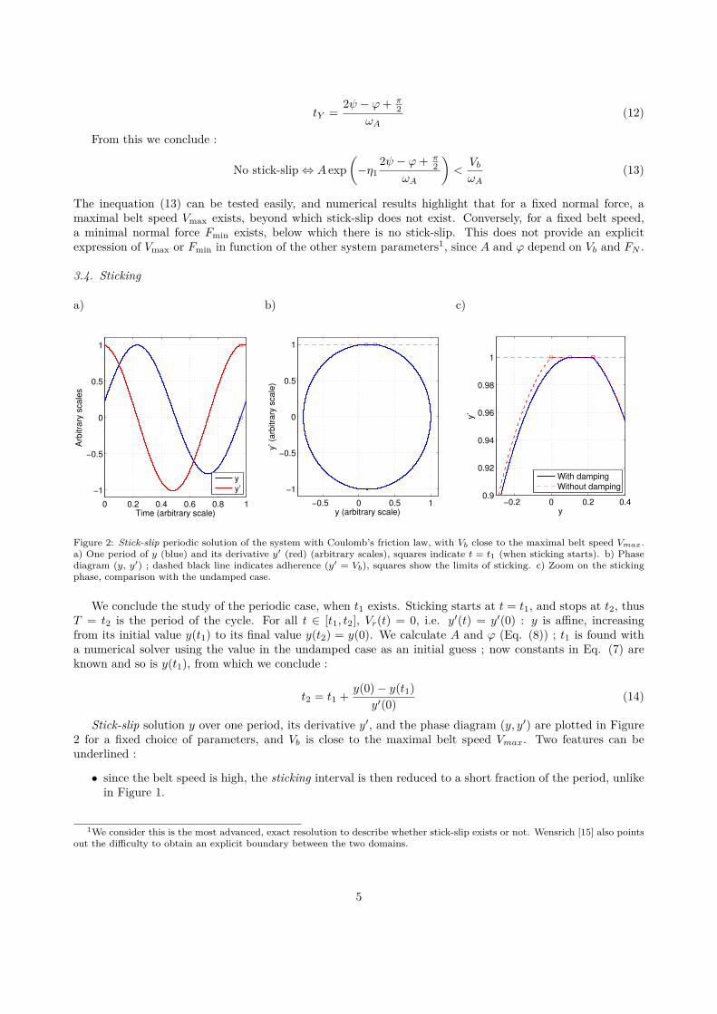
Figure 2: Stick-slip periodic solution of the system with Coulomb’s friction law, with Vb close to the maximal belt speed Vmax.a) One period of y (blue) and its derivative y′ (red) (arbitrary scales), squares indicate t = t1 (when sticking starts). b) Phasediagram (y, y′) ; dashed black line indicates adherence (y′ = Vb), squares show the limits of sticking. c) Zoom on the stickingphase, comparison with the undamped case.

We conclude the study of the periodic case, when t1 exists. Sticking starts at t = t1, and stops at t2, thusT = t2 is the period of the cycle. For all t ∈ [t1, t2], Vr(t) = 0, i.e. y′(t) = y′(0) : y is affine, increasingfrom its initial value y(t1) to its final value y(t2) = y(0). We calculate A and ϕ (Eq. (8)) ; t1 is found witha numerical solver using the value in the undamped case as an initial guess ; now constants in Eq. (7) areknown and so is y(t1), from which we conclude :

t2 = t1 + y(0)− y(t1)y′(0) (14)

Stick-slip solution y over one period, its derivative y′, and the phase diagram (y, y′) are plotted in Figure2 for a fixed choice of parameters, and Vb is close to the maximal belt speed Vmax. Two features can beunderlined :

• since the belt speed is high, the sticking interval is then reduced to a short fraction of the period, unlikein Figure 1.

1We consider this is the most advanced, exact resolution to describe whether stick-slip exists or not. Wensrich [15] also pointsout the difficulty to obtain an explicit boundary between the two domains.

5

• in the phase diagram, the damped solution has an almost horizontal tangent at the end of the slippinginterval, unlike the undamped solution.

We can even compute the bifurcation diagram, for instance over a belt speed interval [V1;V2] (or, similarlya normal force interval) discretized in k + 1 values :

for Vb=[V1 : V2−V1

k : V2]

y(0) = ..., y′(0) = ... (Eq. (6a), (6b))A = ..., ϕ = ... (Eq. (8a), (8b))ψ = ... (Eq. (10b))if inequation (13) is true then no stick-slip

else t1,app = π − 2ϕωA

(t1 in the undamped case serves as an estimate in the damped case)t1 = fsolve(y′(t)− y′(0), start=t1,app)t2 = ... (Eq. (14))

end ifend forThe bifurcation diagram for this non-smooth law may include some non-smooth bifurcations that are not

standard to smooth dynamical systems. This goes beyond the scope of this paper, however the book [16] mayinterest the reader.

4. Regularized friction law

We now present the regularized friction law µn(Vr) used in this paper. It is based on an analytical motherfunction g and a regularization parameter n. This parameter n acts as a scaling factor that modifies thestiffness of the regularization : large values of n mean a highly nonlinear friction law. g is defined as

g(Vr) :=−µdVr

√V 2r + ε− 2αVr

V 2r + 1 , α =

√µs(µs − µd) (15)

where α and ε are fixed parameters. The latter is meant to be small (here, ε = 10−4). The function g isdesigned to verify the following properties :

• g is odd ;

• g(Vr)→ µd when Vr → −∞ ;

• max g → µs when ε→ 0

Then, µn is defined as

µn(Vr) := g(nVr) =−µdVr

√V 2r + ε

n2 − 2αnVrV 2r + 1

n2

(16)

A plot of Coulomb’s law and the regularized law for several values of n, in Figure 3, shows that µn(Vr)resembles Coulomb’s law when n is high. Additional details on the regularization process are given inAppendixA.

We highlight two main differences with Coulomb’s friction law. The first one is a velocity-dependentdynamic coefficient. But as noted by Oden and Martins ([17], p. 548) the assumption of velocity independenceis “now known to be invalid. A large volume of experimental data and empirical formulas for the variation ofthe friction coefficient with sliding velocity can be found”. Yet Coulomb’s law leads to more explicit expressionsof the stick-slip solution, and for non-zero relative speed, it is the limit function of the sequence (µn)n>0.

The second difference is that µn is locally a decreasing function of Vr around Vr = 0, instead of amultivalued coefficient during adherence. This kind of smooth, velocity-dependent friction law, is a modelcommonly used to study the bowed string, from McIntyre and coll. [18] to recent sound synthesis [19]. Thepresent study aims at investigating such a regularized law. More complex models have been designed2, totake into account effects due to rosin [21], string torsion [13], etc.

2Several bowed string models can be found in [20].

6

a)

−1 −0.5 0 0.5 1−0.5

−0.4

−0.3

−0.2

−0.1

0

0.1

0.2

0.3

0.4

0.5

Vr (m.s

−1)

Friction c

oeffic

ient µ

C

Coulomb’s law

b)

−1 −0.5 0 0.5 1−0.5

−0.4

−0.3

−0.2

−0.1

0

0.1

0.2

0.3

0.4

0.5

Vr (m.s

−1)

Friction c

oeffic

ient µ

n

n=10

n=25

n=100

Figure 3: a) Coulomb’s friction law, for µs = 0.4, µd = 0.2. b) Regularized friction µn for n = 10 (black), 25 (blue), 100 (red).

A smooth friction law around 0 allows “no true sticking” (an expression found for example in [22]), adrawback in a purely static context, however the present paper focuses on dynamic phenomena. Frictionregularization has been used to find approximate solutions of variational formulations (for example [23, 17]),but the authors found a small number of papers that use it in numerical simulations expecting realisticfriction :

• Feeny and Moon [24] showed that for a harmonically forced spring-mass system, a smooth friction lawcan reproduce qualitatively the chaotic behaviour observed with Coulomb’s law. The selected smoothfunction reads :

µ(Vr) = (µd + (µs − µd)sech(βVr)) tanh(αVr) (17)

• Quinn [25] proposes a smoothing procedure that respects the multivaluation at null relative speed byintroducing an additional variable. However, it is presented in the case µs = µd, and its adaptation inthe case µs > µd may be delicate.

• Vrande et al. [26] use the function :

µ(Vr) = − 2π

arctan(εVr)1 + γ|Vr|

(18)

where ε is the regularization parameter. The maximal value of µ is not constant when ε varies, and therange of belt speeds is restricted because this function tends to zero when Vr tends to infinity.

5. Periodic solutions using a regularized friction law

We now investigate the periodic solutions with the regularized friction law presented in Section 4. Thenumerical framework used is presented in [9] and [27] and implemented in the Matlab toolbox MANLAB [28].

5.1. Quadratic recastPeriodic solutions, and their continuation with respect to parameters Vb or FN , are studied with a con-

tinuation procedure. A robust method to compute a solution branch is the Asymptotic Numerical Method(ANM). It operates on first-order differential systems with quadratic nonlinearities. This is called a quadraticformulation and requires auxiliary variables to lower the derivation order to 1, and to recast the nonlinearitiesinto quadratic ones, so that Z, the vector of all variables, is solution of

m(Z ′) = c0 + λc1 + l0(Z) + λl1(Z) + q(Z,Z) (19)

7

where λ is the continuation parameter, c0 and c1 are vectors, l0, l1 andm are linear operators, and q is a bilinearoperator [9]. After this quadratic recast, periodic solutions are studied using either the Harmonic BalanceMethod or the Orthogonal Collocation at Gauss points, as implemented in [27] ; unless stated otherwise below,they provide the same results. A detailed study of their convergence should be carried out in a companionpaper [29].

The differential equation (1) on y is transformed into a first-order system on (y, z) :

y′ = ω1z (20)

z′ = −2ζ1ω1z − ω1y + FNω1M1

µn (Vr) where Vr = ω1z − Vb (21)

Then, seeing the definition (16) of µn(Vr), we define three auxiliary variables to obtain quadratic nonlin-earities :

R =√V 2r + ε

n2 (22)

S = V 2r + 1

n2 (23)

µn =−µdVrR− 2αnVr

S(24)

The definition of R is then recasted asR2 = V 2

r + ε

n2 (25)

The latter, (25), is not equivalent to the previous definition, (22), and the positiveness of R has to be checked(this should be studied in a companion paper [29]).

5.2. Continuation with respect to the belt speed

a)

0 2 4 6 8 100

0.002

0.004

0.006

0.008

0.01

0.012

0.014

0.016

0.018

Vb (m.s

−1)

B2

B3B

1

Am

plit

ude (

m)

Helmholtz

Slipping

b)

0 2 4 6 8 101200

1205

1210

1215

1220

1225

1230

1235

Vb (m.s

−1)

B2

B3

Puls

ation (

rad.s

−1)

4 6 8 101231.59

1231.6

1231.61

1231.62

B2

B3

B1

Figure 4: Bifurcation diagram with the continuation parameter λ = Vb, and n = 10, FN = 5 N. The branch is plotted in solidline if it is stable, and dashed otherwise ; Helmholtz motion is in blue, slipping in green. HBM truncation order : H = 70. a)Peak-to-peak amplitude versus the belt velocity. b) Pulsation versus the belt velocity. Natural pulsation ω1 is plotted in purple.A zoom window shows the branch between bifurcations B2 and B3.

A first continuation study is carried out with the belt speed Vb being the continuation parameter λ, whilethe normal force is fixed (FN = 5 N). The quadratic recast, emphasizing the operators of Eq. (19), and basedon Eq. (20), (21), (23), (24) and (25), is :

8

0 = −λ + ω1z − Vr + 0 (26a)

0 = ε

n2 + 0 + V 2r −R2 (26b)

0 = 1n2 − S + V 2

r (26c)

0 = 0 + 2αnVr + µnS + µdVrR (26d)

y′ = 0 + ω1z + 0 (26e)

z′︸︷︷︸m(Z′)

= ︸︷︷︸c0+λc1

0 − 2ζ1ω1z − ω1y + FNω1M1

µn︸ ︷︷ ︸l0(Z)+λl1(Z)

+ ︸ ︷︷ ︸q(Z,Z)

0 (26f)

For n = 10, the bifurcation diagram is given in Figure 4 (left) with stability analysis and movementdescription. Amplitude refers to peak-to-peak amplitude of the displacement y.

The upper stable branch starts with a supercritical Hopf bifurcation (B1 on the diagram) around Vb = 0.14m.s−1, reaching a maximal belt speed (B2) around Vb = 10.25 m.s−1. From there, the lower branch is unstable,and ends on a subcritical Hopf bifurcation (B3) around Vb = 3.65 m.s−1. This stability analysis is performedwith Hill’s method [30]. This method is efficiently combined with the Harmonic Balance Method, providedthat the Jacobian matrix of the nonlinear differential system (y, z)′ = F(y, z) (i.e. Eq. (20), (21)) is alsoquadratically recasted. In our case, this requires three additional variables, which means that the computationof the bifurcation diagram is slightly slowed down, then the stability analysis is almost immediate. This is agood compromise, and is preferred to the integration of the Jacobian matrix over one period to obtain themonodromy matrix, which is much more time consuming.

Some authors consider that using a regularized law prevents any real stick phase (for example, [22, 31]).We refine this by defining the movement type as follows : let Vn be such that µn(Vn) = maxv µn(v), then

|Vr(t)| 6 |Vn| ⇒ stick, |Vr(t)| > |Vn| ⇒ slip (27)

Then, a solution is called either “slipping” if a period contains no sticking interval, or “Helmholtz motion”,if there is exactly one sticking interval and one slipping interval. The plot in Figure (4) can be summed upas : Helmholtz motion on the upper branch, slipping on the lower branch. There are two details : aroundbifurcation B1, the mass is only slipping ; the Helmholtz motion is still present on the lower branch near B2.

We now choose greater values of n, the regularization parameter, namely 25, 50 and 100. The bifurcationdiagram is altered (Figure 5) :

• Hopf bifurcations B1 and B3 happen at lower belt speeds ;

• the maximal belt speed decreases ;

• the amplitude gap between the stable and the unstable branches decreases.

For belt speeds close to the first Hopf bifurcation, the motion amplitude is small and relative speed Vroscillates very slightly around Vn. In other words, µn stays close to its maximum µs. In Coulomb’s case, theamplitude of the stick-slip solution tends to a strictly positive value when the belt speed tends to 0. Thereis a discontinuity at Vb = 0, where the amplitude is zero since there is no motion. Examples of Helmholtzmotion, in the regularized case and in Coulomb’s case, are shown in Figure 6, a.

For Coulomb’s law the pulsation is an increasing function of the belt speed (Figure 8) that tends to 0when the belt speed tends to 0. For the regularized law, pulsation starts at the natural pulsation at B1, thendecreases to similar values to the unregularized case, in a steep way for great values of n. From then on, it isalso a function of Vb increasing towards its final value ω1, reached at the second Hopf bifurcation B3.

With greater values of n (highly nonlinear system), for instance for n = 150, the pulsation steep decreasesnear the first bifurcation B1 ranges over a short interval, while the amplitude is a steep increasing functionof the belt speed. In this interval, it is difficult for numerical methods to find the expected periodic solution.The Harmonic Balance Method predicts an hysteresis over a very short interval ; the size of this interval

9

0 1 2 3 4 5 6 7 80

0.002

0.004

0.006

0.008

0.01

0.012

0.014

Vb (m.s

−1)

Am

plit

ud

e (

m)

0 0.2 0.40

2

4

6

8x 10

−4

n=25

n=50

n=100

Coulomb

B2 (n=50)

B2 (n=25)

B2 (n=100)

Vmax

Figure 5: Bifurcation diagram (axes : belt speed, peak-to-peak amplitude of displacement) with the regularized friction law andn = 25 (black; H = 100), n = 50 (blue; H = 125), n = 100 (red; H = 175) ; with Coulomb’s law (green). The position of thebifurcation points B1, B2 and B3 change for each value of n.The maximal belt speed, examined in Section 3.3, is shown as Vmax.

a)

−4 −2 0 2 4 6

x 10−4

−1

−0.8

−0.6

−0.4

−0.2

0

Displacement y (m)

Rela

tive v

elo

city V

r (m

.s−

1)

n=10

n=25

n=100

Coulomb

b)

−2 0 2 4

x 10−4

−0.06

−0.05

−0.04

−0.03

−0.02

−0.01

0

0.01

0.02

Displacement y (m)

Rela

tive v

elo

city V

r (m

.s−

1)

n=10

n=25

n=100

Coulomb

Figure 6: Phase diagrams, examples of stick-slip, for Vb = 0.5 m.s−1. Regularized law : n = 10, H = 70, black; n = 25, H = 100,blue; n = 100, H = 175, red. Coulomb’s law : green. a) Entire phase diagram. b) Zoom around the sticking part.

diminishes when more harmonics are used (Figure 9). The Orthogonal Collocation at Gauss points [32] doesnot exhibit this behaviour and describes amplitude and pulsation as functions of the continuation parameterVb.

To confirm the continuation results, we can extract a periodic solution (from one of the two bifurcationdiagrams, HBM or Collocation), and start a numerical solver with initial conditions y(0), y′(0). Among thesolvers available in Matlab ODE suite [33] designed for stiff systems, ode15s was found to be reliable andfaster than others on this system. Such a validation is presented for n = 100 in Fig. 7. However, for n = 150and in the Vb interval described above, the absolute error tolerance of the function ode15s (parameter AbsTol)must be set as low as 10−14 (this worsens as n increases since the system becomes stiffer). Otherwise, it does

10

0 1 2 3 4 5

x 10−3

10−14

10−12

10−10

10−8

10−6

t

Absolu

te d

iffe

rences

betw

een H

BM

and O

DE

yV

r

Figure 7: Validation with ode15s of the HBM solution, for n = 100 and H = 175, for Vb = 0.5 m.s−1 : absolute differencesbetween the two solutions, for y and Vr.

not converge to the same periodic solution.

10−2

10−1

100

300

400

500

600

700

800

900

1000

1100

1200

1300

Vb (m.s

−1)

Pu

lsa

tio

n (

rad

.s−

1)

n=25

n=50

n=100

Coulomb

Vmax

Figure 8: Pulsation versus belt speed, with the regularized friction law and n = 25 (black; H = 100), n = 50 (blue; H = 125),n = 100 (red; H = 175) ; with Coulomb’s law (green). Natural pulsation ω1 is drawn in purple. The branch between B2 and B3is not visible at this scale.

5.3. Continuation with respect to the normal forceWe now choose the continuation parameter λ = FN and a fixed belt speed (Vb = 0.2 m.s−1). Changing λ

requires a new quadratic formulation similar to Eqs. (26). It is not given here for sake of brevity.For small values of n, for example n = 10, the bifurcation diagram (Figure 10, a) shows a stable branch

with a supercritical Hopf bifurcation. For higher values of n (n = 25 is enough), the Hopf bifurcation becomessubcritical (Fig. 10, b).

11

a)

9.4928 9.493 9.4932 9.4934

x 10−3

2

4

6

8

10

12

14

x 10−5

Vb (m.s

−1)

Am

plit

ude (

m)

H=100H=150

H=200OC

b)

0 1 2 3 4 5

200

400

600

800

1 000

1 200

Vb (m.s

−1)

Puls

ation (

rad.s

−1)

0.01 0.015 0.02

400

800

1 200

c)

9.4928 9.493 9.4932 9.4934

x 10−3

200

400

600

800

Vb (m.s

−1)

Puls

ation (

rad.s

−1)

H=100

H=150

H=200

OC

Figure 9: For n = 150, comparison of the Harmonic Balance Method with H = 100 (black), 150 (blue), 200 harmonics (red), andOrthogonal Collocation (OC) with Nint = 151 subintervals. a) Peak-to-peak amplitude versus the belt velocity, for the intervalI = [9.4928 × 10−3; 9.4935 × 10−3]. b) Pulsation versus the belt velocity, entire diagram with a zoom window on the interval[0.009; 0.02]. c) Pulsation versus the belt velocity, zoom of the previous one on the interval I = [9.4928 × 10−3; 9.4935 × 10−3],comparison of the HBM and the OC.

Comparisons with Coulomb’s law, for the amplitude (Figure 11) and the pulsation (fig. 12) show aqualitative agreement between regularized law and Coulomb’s law. For either law, the mass can be carriedaway as far as desired during the stick phase, provided that the normal force FN is great enough. This phasebecomes longer when FN increases, and therefore the pulsation decreases. Nevertheless, the agreement isless compelling than for the belt speed continuation. For small values of the regularization parameter n, theamplitude is close to the amplitude occurring with Coulomb’s law. For n = 50 or n = 100 and high valuesof normal force FN , there is still a large difference between pulsation with Coulomb’s law and the one withregularized law.

a)

0 2 4 6 8 10 12 14 160

1

2

3

x 10−4

FN (N)

Am

plit

ude (

m)

Helmholtz

Slipping

b)

0 2 4 6 80

1

2

3

4

5

6x 10

−4

FN (N)

B

B

Am

plit

ude (

m)

0 0.05 0.1 0.15 0.20

1

2

3

4x 10

−4

B

B

Helmholtz

Slipping

Figure 10: Bifurcation diagram with the continuation parameter λ = FN . The branch is plotted in solid line if it is stable, anddashed otherwise ; Helmholtz motion is in blue, slipping in green. a) Weakly nonlinear system, n = 10. HBM truncation order :H = 70. b) Stiff nonlinear system, n = 100. H = 300.

6. Conclusion

In this paper we investigated the periodic solutions of a mass-spring-damper-belt system, and comparedtwo different friction laws, Coulomb’s law and a regularized law. In the Coulomb case, the stick-slip solutionis constructed sequentially, giving access to limit values for the belt speed and the normal force. In theregularized case, the bifurcation diagrams, obtained by numerical continuation with respect to the belt speed

12

0 1 2 3 4 5 6 7 80

1

2

3

4

5

6x 10

−4

FN (N)

Am

plit

ud

e (

m)

n=25

n=50

n=100

Coulomb

Figure 11: Peak-to-peak amplitude versus normal force, with the regularized friction law and n = 25 (black, H = 70), n = 50(blue, H = 150), n = 100 (red, H = 300) ; with Coulomb’s law (green).

0 1 2 3 4 5 6 7 81060

1080

1100

1120

1140

1160

1180

1200

1220

1240

FN (N)

Pu

lsa

tio

n (

rad

.s−

1)

n=25

n=50

n=100

Coulomb

Figure 12: Pulsation versus normal force, with the regularized friction law and n = 25 (black, H = 70), n = 50 (blue, H = 150),n = 100 (red, H = 300) ; with Coulomb’s law (green). Natural pulsation ω1 is shown in purple.

or to the normal force, and for several values of the regularization parameter, fulfilled two goals. They provethe robustness of the association of the Asymptotic Numerical Method and the HBM confronted with a highlynonlinear law; they give a comprehensive description of the stick-slip branch and of the slipping branch, aswell as their evolution when the system becomes highly nonlinear. Formulations from the Coulomb case givethe means of a comparison between the regularized solutions and a standard reference.

13

The present study highlights that several qualitative aspects of friction are preserved with the smoothfunction of relative velocity chosen as the friction law. With an appropriate definition, stick-slip motionexists, its amplitude increases with respect to the belt speed and its pulsation decreases with respect to thenormal force. There are limit values for the belt speed and the normal force beyond which this periodicmotion ceases to exist. However, with the regularized law some unstable branches of solution can exist, andhave no counterpart with Coulomb’s law. For example, the continuation with respect to the belt speed showsa branch of slipping solution.

Thanks to its important nonlinearity, this regularized system serves as a benchmark for our methods oftime discretization. A future companion paper [29] will compare the Harmonic Balance Method and theOrthogonal Collocation at Gauss points, for several values of the regularization parameter n. Future worksbased on this regularized system can feature more complete models, either for the string or the friction law.

Acknowledgements

This work has been carried out in the framework of the Labex MEC (ANR-10-LABX-0092) and of theA*MIDEX project (ANR-11-IDEX-0001-02), funded by the Investissements d’Avenir French Governmentprogram managed by the French National Research Agency (ANR).

AppendixA. Regularization construction

The regularized law µ can be designed as follows : µ is an odd, analytical function, with a (single) maximumvalue µs on R−, and its asymptotic value is µd (when Vr → −∞). The definition

∀ Vr 6 0, µ(Vr) = −µdV2r − 2αVr

V 2r + 1 , (A.1)

verifies our constraints, provided that α =√µs(µs − µd). Since Vr 6 0 with Coulomb’s law, it may seem

sufficient to define µ with Eq. (A.1). Yet, using this definition, numerical simulation shows that Vr does notstay negative over one period, for large intervals of belt speed and normal force. Since the expression given inEq. (A.1) is not odd, the friction coefficient is incorrect over a fraction of the period. A satisfying replacementwould be, for all Vr

µ(Vr) = −µdVr|Vr| − 2αVrV 2r + 1 (A.2)

Unfortunately the modulus |Vr| in Eq. (A.2) is not smooth enough for the continuation study, so wechoose

√V 2r + ε instead. The constant α gives the correct maximum µs only for ε = 0, and small values

of ε engender slightly exaggerated values for the maximum. Numerically, the difference between the smoothfunction g, defined in Eq. (15), and the function µ defined in Eq.(A.2), is one order of magnitude smaller thanε. Thus, the chosen value ε = 10−4 in this paper gives g a maximum value of 0.4 + 10−5, close to µs = 0.4,as shown in figure A.13 by computing the difference between g and µ.

AppendixB. Jacobian matrix

The first-order differential system (Eqs. (20), (21)) reads(yz

)′=(F1(y, z)F2(y, z)

):=(

ω1z−2ζ1ω1z − ω1y + FN

ω1M1µn

)(B.1)

The partial derivatives of F1 and F2 are

∂F1

∂y= 0, ∂F1

∂z= ω1 (B.2a)

∂F2

∂y= −ω1,

∂F2

∂z= −2ζ1ω1 + FN

ω1M1

dVrdz

dµn(Vr)dVr

(chain rule) (B.2b)

14

−2 −1.5 −1 −0.5 0 0.5 1 1.5 210

−9

10−8

10−7

10−6

10−5

10−4

Vr

Diffe

ren

ce

be

twe

en

µ a

nd

g

Figure A.13: Absolute difference between the smooth function g, defined in Eq. (15), and the function µ defined in Eq.(A.2),for ε = 10−4.

where

dVrdz = ω1,

dµnVr

= 1S

(−µdR− µd

V 2r

R− 2α

n− 2Vrµn

)(B.3)

Three auxiliary variables are defined:

UR = V 2r

R, US = 1

S, UM = Vrµn (B.4)

The Jacobian matrix of system (B.1) can then be written with the following constant, linear and quadraticalmatrices:(

0 ω1−ω1 −2ζ1ω1

)+(

0 00 −2FNα

M1nUS

)+ FNM1

(0 00 −µdUSR− µdUSUR − 2USUM

)(B.5)

References

[1] B. Feeny, A. Guran, N. Hinrichs, K. Popp. A historical review on dry friction and stick-slip phenomena,ASME Applied Mechanics Review 51 (5), p. 321-341, 1998.

[2] A. Papinniemi, J.C.S. Lai, J. Zhao, L. Loader. Brake squeal: a literature review, Applied Acoustics 63, p.391-400, 2002.

[3] L. Gaul, R. Nitsche. The role of friction in mechanical joints. Applied Mechanics Review, 54 (2), p. 93-106,2001.

[4] A. Akay. Acoustics of friction, Jounal of the Acoustical Society of America, 111 (4), p. 1525-1548, 2002.

[5] E. Schoonderwaldt, K. Guettler, A. Askenfelt. An empirical investigation of bow-force limits in the Schel-leng diagram, Acta Acustica united with Acustica, 94, p. 604–622, 2008.

15

[6] J. Woodhouse, P.M. Galluzzo. The bowed string as we know it today, Acta Acustica united with Acustica90, p. 579-589, 2004.

[7] O. Inácio, J. Antunes. A linearized modal analysis of the bowed string, Proceedingsof the International Congress of Acoustics. SEA, Madrid. 2007. URL <http://www.sea-acustica.es/WEB_ICA_07/fchrs/papers/mus-04-002.pdf> (accessed 17 March 2016)

[8] P. Vigué, B. Cochelin, S. Karkar, C. Vergez. Investigation of periodic solutions of a bowed string toy model,in M02 Mini symposium Mécanique des Instruments de Musique, Association Française de Mécanique,2015. URL <http://hdl.handle.net/2042/56983> (accessed 17 March 2016)

[9] B. Cochelin, C. Vergez. A high order purely frequency-based harmonic balance formulation for continuationof periodic solutions, Journal of Sound and Vibration, 324, p. 243-262, 2009.

[10] S. Karkar, B. Cochelin, C. Vergez. A high-order, purely frequency based harmonic balance formulationfor continuation of periodic solutions: The case of non-polynomial nonlinearities, Journal of Sound andVibration, 332, p.968-977, 2013.

[11] E. Pennestri, V. Rossi, P. Salvini, P. P. Valentini. Review and comparison of dry friction force models,Nonlinear Dynamics, p. 1-17, 2015.

[12] D. Karnopp. Computer simulation of stick-slip friction in mechanical dynamic systems, Journal of Dy-namic Systems, Measurement and Control, 107 (1), p. 100-103, 1985.

[13] R. I. Leine, D. H. Van Campen, A. De Kraker, L. Van Den Steen. Stick-slip vibrations induced byalternate friction models, Nonlinear Dynamics 16, p. 41-54, 1998.

[14] U. Andreaus, P. Casini. Dynamics of friction oscillators excited by a moving base and/or driving force,Journal of Sound and Vibration, 245 (4), p. 685-699, 2001.

[15] C. Wensrich. Slip-stick motion in harmonic oscillator chains subject to Coulomb friction, Tribology In-ternational, 39, p. 490-495, 2006.

[16] R. I. Leine, H. Nijmeijer. Dynamics and bifurcations of non-smooth mechanical systems, Lecture Notesin Applied and Computational Mechanics, vol. 18, Springer, 2004.

[17] J. T. Oden, J. A. C. Martins. Models and computational methods for dynamic friction phenomena,Computer methods in applied mechanics and engineering 52, p. 527-634, 1985.

[18] M. E. McIntyre, R. T. Schumacher, J. Woodhouse. On the oscillations of musical instruments, Journalof the Acoustical Society of America, 74, p. 1325–1345, 1983.

[19] C. Desvages, S. Bilbao. Physical modeling of nonlinear player-string interactions in bowed string soundsynthesis using finite difference methods, Proceedings ISMA, p. 261-266, 2014.

[20] J. Woodhouse. Idealised models of a bowed string, Acustica 79, p. 233-250, 1993.

[21] J. H. Smith, J. Woodhouse. The tribology of rosin, Journal of the Mechanics and Physics of Solids, 48,p. 1633-1681, 2000.

[22] E. J. Berger. Friction modeling for dynamic system simulation, Applied Mechanics Review, 55, 6, p.535-577, 2002.

[23] J. A. C. Martins, J. T. Oden. A numerical analysis of a class of problems in elastodynamics with friction,Computer Methods in Applied Mechanics and Engineering, 40, p. 327-360, 1983.

[24] B. Feeny, F. C. Moon. Chaos in a forced dry-friction oscillator : experiments and numerical modelling,Journal of Sound and Vibration, 170 (3), p. 303-323, 1994.

[25] D. D. Quinn. A new regularization of Coulomb friction, Journal of Vibration and Acoustics, 126, p.391-397, 2004.

16

[26] B. L. Van De Vrande, D. H. Van Campen, A. De Karker. An approximate analysis of dry-friction-inducedstick-slip vibrations by a smoothing procedure, Nonlinear Dynamics, 19, p. 157-169, 1999.

[27] S. Karkar, C. Vergez, B. Cochelin. A comparative study of the harmonic balance method and the orthog-onal collocation method on stiff nonlinear systems, Journal of Sound and Vibration, 333, 12, p.2554-2567,2014.

[28] S. Karkar, R. Arquier, B. Cochelin, C. Vergez, A. Lazarus, O. Thomas, MANLAB, An InteractiveContinuation Software. URL <http://manlab.lma.cnrs-mrs.fr> (accessed 17 March 2016)

[29] P. Vigué, C. Vergez, S. Karkar, B. Cochelin. Regularized friction and continuation : A comparative studyof the harmonic balance method and the orthogonal collocation method, to be submitted.

[30] A. Lazarus, O. Thomas. A harmonic-based method for computing the stability of periodic solutions ofdynamical systems, Comptes Rendus Mecanique 338, p. 510-517, 2010.

[31] K. Popp, N. Hinrichs, M. Oestreich. Analysis of a self excited friction oscillator, Dynamics with Friction:Modeling, Analysis and Experiments, p. 1-35, World Scientific Publishing Company.

[32] C. de Boor, B. Swartz. Collocation at Gaussian points, SIAM Journal of Numerical Analysis, 10, p.582-606, 1973.

[33] L.F. Shampine, M.W. Reichelt. The Matlab ODE suite, SIAM Journal on Scientific Computing, 18, p.1–22, 1997.

17