Quantitative Finance, 2010, 1–11, iFirst

Real options with a double continuation region

ANNA BATTAUZy, MARZIA DE DONNOz and ALESSANDRO SBUELZ*xyDepartment of Finance, Bocconi University, Milan, Italy

zDepartment of Decision Sciences, Bocconi University, Milan, ItalyxDepartment of Mathematics, Quantitative Finance, and Econometrics,

Catholic University of Milan, Milan, Italy

(Received 26 April 2008; revised 6 April 2010; in final form 6 April 2010)

If the average risk-adjusted growth rate of the project’s present value V overcomes thediscount rate but is dominated by the average risk-adjusted growth rate of the cost I ofentering the project, a non-standard double continuation region can arise: The firm waits toinvest in the project if V is insufficiently above I as well as if V is comfortably above I. Under aframework with diffusive uncertainty, we give exact characterization to the value of the optionto invest, to the structure of the double continuation region, and to the subset of theprimitives’ values that support such a region.

Keywords: Asset pricing; American options; Capital investment theory; Optimal stopping;Free boundary

1. Introduction

The problem of optimal irreversible investment in a long-lived project has usually been studied under the assump-tion that the average risk-adjusted growth rate of theproject’s present value is dominated by the discount rate(for instance, see the classical textbook of Dixit andPindyck 1993, pp. 138–141 and p. 211). This assumptionis standard and serves the purpose of avoiding anexplosive value for the perpetual option to invest. Theassumption leads to the standard continuation region:The firm waits to invest if the project’s present value Vinadequately exceeds the unrecoverable cost I of enter-ing it. Our first contribution is to show that such anassumption is conspicuously restrictive. In the presence ofa stochastic cost I, the assumption rules out cases in whichthe value of the investment option does not explode. Oursecond contribution is to show that such uncharted casesare extremely interesting. They can give rise to a non-standard double continuation region: The firm waits toinvest if V is insufficiently above I as well as if V iscomfortably above I. To the best of our knowledge, thisimportant result is novel in the literature on investmentunder uncertainty. Our third contribution is to provide arigorous and explicit description of the firm’s optimal

decision in these unexplored cases. We use a setting withdiffusive uncertainty to accurately characterize the ana-lytical value of the option to invest, the structure of thedouble continuation region, and the subset of the prim-itives’ values that support such a region. We offernumerical evidence that natural levels of businessgrowth and risk, of prices of risk, and of discount ratecan lead to the double continuation region.

The intuition behind our results is strikingly uncom-plicated, as the following example shows. Under thevaluation probability measure P, take the present value Vto be a geometric Brownian motion (the default assump-tion in the real-options literature) with a percentage driftof 6% per annum and take the discount rate to be 5%.If the cost I is constant, the problem is unbounded. Givenany initial level for V, the firm finds it optimal topostpone investment to the furthest future as an unlimitedexpected discounted gain can be reaped by doing so.However, if the cost I is a geometric Brownian motion(possibly correlated with V ) with a percentage drift of 7%per annum,y the problem becomes bounded. The cost willeventually overwhelm the value if there is an indefinitepostponement of investment. Optimal postponementbecomes definite, as it applies only in a distinct regionof the initial levels for V and I. The standard part of the

*Corresponding author. Email: alessandro.sbuelz@unicatt.ityAlthough they do not explicitly appear, the correlations between V and I and their local volatilities contribute towards defining theP drifts via the price(s) of risk and the associated risk adjustment.

Quantitative FinanceISSN 1469–7688 print/ISSN 1469–7696 online � 2010 Taylor & Francis

http://www.informaworld.comDOI: 10.1080/14697688.2010.484024

Downloaded By: [Sbuelz, Alessandro] At: 12:50 20 December 2010

region is located where the initial V either does not exceedthe initial I or insufficiently exceeds it. Notably, the non-standard part of the region is located where the initial Vcomfortably exceeds the initial I. Discounted values andcosts have positive percentage drifts (1% and 2%,respectively). If the initial V tops the initial I largelyenough, delaying the investment is optimal as, over theshort/medium run, the discounted value exhibits a totalaverage increase greater than the discounted cost’s totalaverage increase. This is best seen by fixing the initialvalue V0 to 5 and the initial cost I0 to 1 and by consideringthe suboptimal ‘European-style’ investment strategy ofaccessing the project exactly one year from the initialdate. Jensen’s inequality implies that such a suboptimalstrategy outperforms the strategy of immediateinvestment:

EP½e�0:05�1ðV1 � I1Þþ j F 0�� e�0:05�1ðEP½V1 j F 0� � EP½I1 j F 0�Þþ¼ 5 � e0:01�1 � 1 � e0:02�1¼ 4:034V0 � I0,

where EP denotes expectationy under the probabilitymeasure P. The straightforward implication is that thestrategy of immediate investment is also suboptimal. Thenumerical example offers brazen evidence that plausiblelevels of the real-option primitives can lead to the non-standard optimal decision of continuing to hold a realoption that is deep in-the-money.

Under the assumption that both V and I are diffusions,we start as in Aase (2005)z by describing the primitives(business growth, business risk, prices of risk, anddiscount rate) under the historical probabilitymeasure P. We then tackle the optimal investmentproblem by transiting to a valuation probability measureP. If V and I are spanned by traded assets, the prices ofrisk are dictated by the market, the discount rate equalsthe risk-free rate, and P corresponds to a martingalemeasure. Even under a martingale measure P, V and I caneasily grow at an average rate different from the risk-freerate, since V and I are unlikely to match the values oftraded self-financing portfolios at any point in time. Inparticular, V and I can grow on average more than therisk-free rate and at different speeds. Hence, the spanningcondition is easily congruent with the uncharted cases weare focusing on in the present work.

In general, we do not restrict our analysis to anyparticular choice of the valuation measure. We allow forsubjective prices of risk, which are used by the firm torisk-adjust future cashflows from the considered business.We also allow for a subjective discount rate, which is used

by the firm to discount risk-adjusted future cashflows.

We arrive at closed formulae via a change of numeraire

that reduces our problem to the valuation of an American

perpetual put option on the cost-to-value ratio with an

endogenous ‘deflating rate’ that depends on the primi-

tives’ values and that can be either positive or negative.

Importantly, our ability to arrive at an analytical solution

of the investment problem does not depend on the

change-of-numeraire technique. The investment problem

can be fully solved even without slashing its two value-

and-cost dimensions to the single cost-to-value dimen-

sion. However, passing from a problem written in V and

in I to a reduced-form problem written in the ratio I/V

greatly improves the comparability of our results with the

existing literature. Change-of-numeraire techniques for

American options have been used by Battauz (2002) and

by Carr (1995) for the finite-maturity case. Carr (1995)

explicitly applies his results to capital investment theory,

formalizing early dimension-reducing practices reviewed

by Dixit and Pindyck (1993) in the context of that theory.The double continuation region is a novel result that

contributes to the real-options literature. By starting from

a fairly unrestricted structural problem under P and then

moving to its reduced form, we heighten the economic

flexibility of our approach. In turn, such flexibility

empowers the uncovering of unsuspected but artless

combinations of the structural parameters under which,

even when the investment option is deep in-the-money,

V and I can have a relative growth that makes the

(bounded) present value of waiting to invest greater than

the immediate-investment value.Discounting is the perfect terrain for spotting the

difference between the traditional assumptions on the

real options parameters and the combination of structural

parameters that enables the double continuation region.

A non-negative ‘deflating rate’ is applied to the value-to-

cost ratio by Dixit and Pindyck (1993, p. 211). In contrast,

the sign of the endogenous ‘deflating rate’ that we apply to

the cost-to-value ratio is determined by the relative size of

the primitives. If such a sign is negative (the subjective

discount rate is dominated by the value’s average risk-

adjusted growth rate) and if the cost’s average risk-

adjusted growth rate dominates the value’s one, our

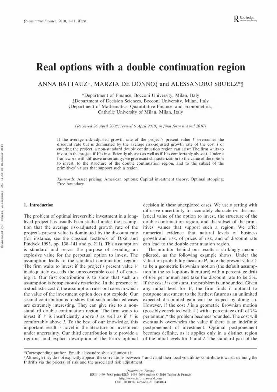
novel result ensues: The firm waits to invest if V over I is

low enough as well as if V over I is high enough. Hence,

in the plane [I,V], the early exercise region must be

straddled by the double continuation region,x as shown

in figure 1.The derivation of our results gives a technical contri-

bution to the real-options literature by adapting the

classical verification theorem (for the jump-diffusion case,

yConditioning the expectation upon F 0 is intended to stress the dependence of the resulting quantities on the initial values forV and I.zAase (2005) highlights the key role played by risk adjustment for an American perpetual option pricing problem, and works outexact solutions when jump sizes cannot be negative. He investigates when his solution is an approximation also for negative jumps.xBroadie and Detemple (1997) and Detemple (2006) have shown that a single continuation region surrounded by multipleimmediate-exercise regions arises with a variety of finite-maturity American derivatives written on two or more traded riskyunderlying assets. Battauz et al. (2009) investigate the double continuation region in a number of finite-maturity American problems.

2 A. Battauz et al.

Downloaded By: [Sbuelz, Alessandro] At: 12:50 20 December 2010

see, for example, Mordecki 1999 and Øksendal and Sulem2004) and by extending it to the situation of a non-integrable ‘deflated’ value function. Such a situation isoriginated by a negative ‘deflating rate’ and belongs tothe non-standard cases we treat in the present work.Not surprisingly, it is associated with the possibleemergence of the double continuation region.

The article is organized as follows. Section 2 introducesthe investment problem and its primitives. Section 3describes the endogenous ‘deflating rate’ in the reduced-form problem. Section 4 uses convexity, monotonicity,and value dominance to discuss the emergence of thedouble continuation region. In theorem 4.1 we providethe exact structure of the double continuation region.Section 5 collects numerical and graphical examples of thedouble continuation region. Section 6 concludes.

2. The investment problem and its primitives

Uncertainty is described by the historical probabilityspace (�,P, (F t)t), and by two independent Brownianmotions WP and eWP. The two Brownian motionsrepresent the diffusive risk that affects value and cost.The present value V of the project has P dynamics:

dVt ¼ Vt

��V dtþ �V dWP

t þe�V deWPt

�,

where �V, �V, and ~�V are real positive constants. Theinvestment cost I has P dynamics:

dIt ¼ Itð�I dtþ �I dWPt Þ,

where �I and �I are real positive constants. The currentvalue of the perpetual option to invest is

sup��0

EP½e���ðV� � I�Þþ j F 0�, ð1Þ

where � is the constant subjective discount rate, and theexpectation is taken under the valuation measure P.Problem (1) consists of finding the optimal exercise policyfor a perpetual American call option on the asset value Vwith a non-constant strike I. The supremum in

problem (1) runs among all stopping times �. The optimaltime to invest is the stopping time �� that attains thesupremum in problem (1). The attained supremum is thevalue function and constitutes a Snell envelope, as it is thesmallest supermartingale majorant of the discountedpayoff from investing.

Given the subjective prices of W-type risk (�) and ofeW-type risk (e�), the P dynamics of V and I can bederived by employing classical Cameron–Martin–Girsanov results for diffusion processes (see, for example,Protter (2004)):

dVt ¼ Vt

�ð�V þ �V� þe�Ve�Þ dtþ �V dWP

t þe�V deWPt

�and

dIt ¼ It�ð�I þ �I�Þ dtþ �I dW

Pt

�,

where WP and eWP are independent Brownian motionsunder P. If � ¼e� ¼ 0, all the subjective prices of risk arenull and the firm is risk-neutral (P ¼ P). If �50 ande�5 0, the firm is averse to W-type risk and to eW-typerisk. If V and I are spanned by traded assets, the prices ofrisk f�,e�g correspond to the market ones, the discountrate � equals the risk-free rate r, and P becomes amartingale measure. However, it is well known that Vte

�rt

and Ite�rt are P-martingales only if Vt and It coincide with

the values of traded self-financing portfolios at any date t,which is seldom the case for real asset values. It followsthat, even under the spanning condition, the risk-adjustedpercentage drifts of V and I typically differ from thediscount rate:

�V þ �V� þe�Ve� 6¼ �,�I þ �I� 6¼ �:

The choice of the risk-attitude parameters � and e� fixesthe valuation probability measure P for the assessment ofthe real option value in problem (1).

3. The endogenous ‘deflating rate’

We reduce the option-value calculation in problem (1) toa one-dimensional problem by taking the process Vte

�kVt

as numeraire, where

kV ¼ �V þ �V� þe�Ve� � �: ð2Þ

The endogenous coefficient kV is V’s average growth rateunder P, in excess of the subjective discount rate �.Analogously, we have that kI,

kI ¼ �I þ �I���, ð3Þis I ’s average growth rate under P, in excess of �.

The change-of-numeraire techniquey enables a usefuldimension reduction of our investment problem.We denote by PA the auxiliary probability measureassociated with the numeraire Vte

�kVt and re-express theinvestment option value in the following proposition.

0 1 2 30

1

2

3

cost I

Proj

ect v

alue

V

Early

exe

rcise

regi

on

Continuatio

n region

Con

tinua

tion

regi

onV = I

Figure 1. The double continuation region in the plane [I,V].

ySee, for example, Geman et al. (1995) and Battauz (2002) for a comprehensive application of change-of-numeraire techniques toAmerican options.

Real options with a double continuation region 3

Downloaded By: [Sbuelz, Alessandro] At: 12:50 20 December 2010

Proposition 3.1: Problem (1) admits the followingrepresentation:

sup��0

EP½e���ðV� � I�Þþ j F 0� ¼ V0 � vðX0Þ, ð4Þ

with

vðX0Þ ¼ sup��0

EPA ½e�ð�kVÞ�ð1� X�Þþ j F 0� ð5Þ

and

Xt ¼ ItVt

:

Equations (4) and (5) relate the investment optionvalue to the value,y calculated under the auxiliaryprobability measure PA, of an American put optioncharacterized by a unit strike price and written on anunderlying item whose value is the cost-to-value ratio.The payoff from put option exercise is deflated by theendogenous ‘deflating rate’ �kV.

The structure of the cost-to-value ratio under theprobability measure P

A can be derived by again employ-ing the Cameron–Martin–Girsanov results:

Xt ¼ X0 expðatþ �BBtÞ,where Bt is a Brownian motion under PA, and

�2B ¼ ð�I � �VÞ2 þe�2

V,

a ¼ kI � kV � �2B

2:

4. Option value properties and the structure of the

continuation region

Given X’s structure and

X0 ¼ x,

the American put value can be written as

vðxÞ ¼ supu�0

EPA ½e�ð�kVÞuð1� X0 expða � uþ �BBuÞÞþ j F 0�,

ð6Þwhere u runs among the stopping times. The function v(x)inherits convexity and monotonicity from the exer-cise payoff, so that v(x) is convex and monotonicdecreasing in x. By construction, v(x) dominates theexercise payoff:

0 � ð1� xÞþ � vðxÞ � vð0Þ,for any non-negative value of x, where the last inequalitystems from monotonicity. We now adapt the argumentsof Lamberton and Lapeyre (1996) to show how convexity,monotonicity, and value dominance interact with the signof the endogenous ‘deflating rate’ �kV in yielding thedouble continuation region.

When the ‘deflating rate’ is non-negative, that is

�kV� 0, problem (1) is reduced to the valuation of a

standard perpetual American put option with non-

negative interest rates. A standard continuation region

emerges: The firm waits to invest in the project if V is

insufficiently above I.When the ‘deflating rate’ is negative, i.e. �kV50,

a non-standard double continuation region can emerge:

The firm waits to invest in the project if V is insufficiently

above I as well as V is comfortably above I. Indeed, the

put value’s supremum when the underlying is zero is

infinite:

vð0Þ ¼ supu�0

EPA ½e�ð�kVÞuð1� 0Þþ j F 0� ¼ e�ð�kVÞ1 ¼ þ1

4 ð1� 0Þþ:

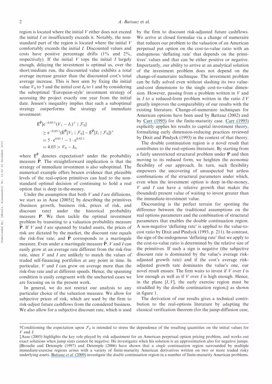
If the value v(x) strictly dominates the exercise payoff

(1�x)þ for all x40 (in figure 2, see the light-colored

dashed line that starts from þ1), early exercise is never

optimal. However, the put value can also land on the

exercise payoff for some x0 belonging to the interval (0, 1).

If it does so, it must remain grounded at the exercise

payoff for a while and then take off from it for

x sufficiently large (see the black solid line in figure 2).

Hence, there exist two critical levels x1 and x2,

x1 ¼ inffx � 0 : vðxÞ ¼ 1� xg,x2 ¼ supfx � 0 : vðxÞ ¼ 1� xg,x1 � x2,

such that there is optimal early exercise only for

x1� x� x2. The non-standard double continuation

region emerges. It is formed by all x5x1 and x4x2,

straddling the early exercise region.We remark that the arguments employed (convexity,

monotonicity, and value dominance) do not depend on

the dynamics of the underlying process X. This is

suggestive that the robustness of the central result of

our work (the surfacing of the double continuation

region) under rather general types of uncertainty is quite

plausible. The numerical and graphical output of section 5

exemplifies the emergence of the double continuation

region.

0.0 0.2 0.4 0.6 0.8 1.00.0

0.5

1.0

Cost-to-value ratio

Figure 2. Put value with �kV50.

yFor an extensive review of valuation methods for American-style claims, see, for example, Broadie and Detemple (2004).

4 A. Battauz et al.

Downloaded By: [Sbuelz, Alessandro] At: 12:50 20 December 2010

In theorem 4.1 we work out an exact characterization

for the values of the option to invest, for the structure of

the double continuation region, and for the subset of the

primitives’ values that support such a region. This is done

via the explicit solutions to problem (1). With this aim, we

adapt and extend the verification theorem as recounted in

lemma 1 of Mordecki (1999). Lemma 1 of Mordecki

(1999) states five standard optimality properties that,

once satisfied by a function, render the function the value

of a perpetual American option on the exponential of a

jump-diffusion process. In our case, the assumed absence

of jumps streamlines the structure of lemma 1. Mordecki

(1999) starts from a reduced-form problem with zero

‘deflating rate’. In theorem 4.1, we contribute by extend-

ing the streamlined lemma 1 to account for a negative

‘deflating rate’. An extension of lemma 1 is required and

not just an adaptation, as one of the five standard

optimality properties (property (IV) in Mordecki’s nota-

tion) is structurally violated. Such a property involves the

integrability of the ‘deflated’ value function for any

exercise policy and is clearly broken by the presence of a

negative ‘deflating rate’, for which we have just seen that

v(0)¼þ1.As mentioned above, there are good reasons to believe

that theorem 4.1’s key economic finding (the materializa-

tion of the double continuation region) is resilient to a

variety of stochastic settings, including environments with

discontinuities. However, eschewing the presence of

jumps enables a thrifty and agile structure for our

theorems and proofs, which significantly enhances the

visibility of our economic contribution to investment and

decision making.

Theorem 4.1 : Assume that

�kV 5 0: ð7Þ

(1) If

kI � kV ¼ aþ �2B

2� 0, ð8Þ

then

V0 � sup��0

EPA

e�ð�kVÞ� 1� I�V�

�þ� �����F 0

" #¼ þ1,

and the corresponding optimal stopping time is

�� ¼ þ1:

(2) Ify

a�ffiffiffiffiffiffiffiffiffiffiffiffiffi2�2

BkV

q4 0, ð9Þ

then equation (in the unknown p)

1

2�2Bp

2 þ apþ kV ¼ 0 ð10Þ

has two negative solutions �25�1:

�2 ¼�a�

ffiffiffiffiffiffiffiffiffiffiffiffiffiffiffiffiffiffiffiffiffiffiffia2 � 2�2

BkVp

�2B

,

�1 ¼�aþ

ffiffiffiffiffiffiffiffiffiffiffiffiffiffiffiffiffiffiffiffiffiffiffia2 � 2�2

BkVp

�2B

:

We have

V0 � sup��0

EPA

e�ð�kVÞ� 1� I�V�

�þ� �����F 0

" #

¼

I�10

V�1�1

0

ð1��1Þ�1�1

ð��1Þ�1, if I0

V05 �1

�1�1 ,

V0 � I0, if �1�1�1 � I0

V0� �2

�2�1 ,

I�20

V�2�1

0

ð1��2Þ�2�1

ð��2Þ�2, if I0

V04 �2

�2�1 :

8>>>>><>>>>>:ð11Þ

and the corresponding optimal stopping time is

�� ¼ inf t � 0 :�1

�1 � 1� It

Vt� �2

�2 � 1

� :

(3) If

a�ffiffiffiffiffiffiffiffiffiffiffiffiffi2�2

BkV

q¼ 0, ð12Þ

then equation (10) has one negative solution �0:

�0 ¼ �ffiffiffiffiffiffiffiffi2kV

p�B

:

We have

V0 � sup��0

EPA

e�ð�kVÞ� 1� I�V�

�þ� �����F 0

" #

¼I�00

V�0�1

0

ð1��0Þ�0�1

ð��0Þ�0, if I0

V06¼ �0

�0�1 ,

V0 � I0, if I0V0

¼ �0�0�1 ,

8><>: ð13Þ

and the corresponding optimal stopping time is

�� ¼ inf t � 0 :ItVt

¼ �0�0 � 1

� :

The proof of theorem 4.1 is given in the appendix.The condition of a negative ‘deflating rate’ in (7)

violates the standard assumption in the literature on

investment under uncertainty. It implies that, under the

valuation measure P, V’s percentage drift dominates the

discount rate �. However, as points 2 and 3 of theorem 4.1

make clear, such a violation does not always lead to an

infinite value of the investment opportunity, but instead

opens the way to uncharted non-explosive cases of

remarkable interest.In point 1, condition (8) is conducive to the explosive

solution. The percentage PA-drift of the cost-to-value

ratio processfIt/Vt)}t�0 is given by aþ ð�2B=2Þ. Its non-

positivity implies that, by Jensen’s inequality,

yNotice that a40 implies kI� kV40.

Real options with a double continuation region 5

Downloaded By: [Sbuelz, Alessandro] At: 12:50 20 December 2010

delaying perpetually access to the payoff

e�ð�kVÞt½1� ðIt=VtÞ�þ becomes optimal.In points 2 and 3, conditions (9) and (12) grant that X

has a sufficiently high rate of growth to counteract the

effect of the negative ‘deflating rate’, resulting in a finite

value for the put option.In point 2, condition (9) keeps the problem bounded by

ensuring that equation (10) admits two negative solu-

tionsy �14�2. In turn, this ensures that the process

fe�ð�kVÞtvðIt=VtÞgt�0 is a PA-martingale in the continuation

region and a PA-supermartingale in the early exercise

region.In point 3, the immediate investment region collapses

into a singleton, which represents the tangency point

between the early exercise payoff and the put option

value.

5. Examples of the double continuation region

In this section, we offer numerical evidence that credible

levels of business growth and risk, of prices of risk, and of

discount rate can lead to the double continuation region

described in points 2 and 3 of theorem 4.1. Consider the

values for the primitive parameters shown in table 1.

These parameter values imply that the conditions in

point 2 of theorem 4.1 are satisfied with

�1 ¼ �1:08774 �2 ¼ �1:9123:

The American put value v(I/V ) (see equation (6)) is

plotted versus the cost-to-value ratio I/V in the left-hand

plot of figure 3. Optimal immediate investment occurs in

the cost-to-value zone

�1�1 � 1

¼ 0:5210 � I

V� 0:6566 ¼ �2

�2 � 1:

Fixing the cost I to 1 without loss of generality, the

double continuation region is the union of the project-

value zones

V5�2 � 1

�2¼ 1:5229, 1:9194 ¼ �1 � 1

�15V:

The value V � v(1/V ) of the corresponding option to invest

(see formula (11)) is plotted versus the project’s present

value V in the right-hand plot of figure 3.Coeteris paribus, we now take the discount rate to be

�¼ 4.46875%. The conditions in point 3 of theorem 4.1

are satisfied with

�0 ¼ �1:5:

The American put value v(I/V ) is plotted versus the cost-

to-value ratio I/V in the left-hand plot of figure 4.

Optimal immediate investment occurs only for a single

cost-to-value ratio level:

I

V¼ �0

�0 � 1:

Fixing I to 1, the double continuation region swamps thewhole real line but for a singleton:

V 6¼ �0 � 1

�0¼ 1:6667:

The value V � v(1/V ) of the corresponding option to investis plotted versus the project’s present value V in the right-hand plot of figure 4.

6. Conclusions

We have performed a thorough analysis of optimalirreversible investment in a long-lived projectz when itspresent value V and its cost I are two possibly correlateddiffusions. By removing the standard assumption that theaverage growth rate of the project’s present value isalways dominated by the discount rate under the valua-tion measure, we uncover the emergence of a non-standard double continuation region: The firm waits toinvest if V is insufficiently above I as well as if V iscomfortably above I.

Such a non-standard region emerges when the dis-counted value has an average growth rate that is positivebut smaller than the discounted cost’s one. The intuitionbehind our novel results is transparent. If the initial Vtops the initial I largely enough, delaying the investment isoptimal since, over the short/medium run, the discountedvalue exhibits a total average increase greater than thediscounted cost’s total average increase.

We start by describing the primitives (business growth,business risk, prices of risk, and discount rate) under thehistorical probability measure and then we tackle theoptimal investment problem by transiting to a valuationprobability measure. We argue that a double continuationregion can occur even if V and I are spanned by tradedassets, that is, even if the valuation measure is amartingale measure. We obtain closed formulae for theinvestment-option value by means of a change of

Table 1. Values for the primitive parameters.

Risk

W-type risk eW-type risk

Growth�V¼ 25% �V¼ 20% e�V ¼ 25%�I¼ 30% �I¼ 20%

Discount rate Price of risk�¼ 5% �¼� 30% e� ¼ �30%

yThe negative exponents �1 and �2 guarantee that the investment option value expressed in equation (11) remains increasing in V anddecreasing in I also in the continuation region.zThe project’s predictable demise is considered in the real-options analysis of Magis and Sbuelz (2006).

6 A. Battauz et al.

Downloaded By: [Sbuelz, Alessandro] At: 12:50 20 December 2010

numeraire that reduces our problem to the assessmentof an American perpetual option on the cost-to-valueratio.

The change of numeraire leads to a one-dimensionalreduced-form problem whose comparability with theexisting literature is strongly enhanced. However, ourresults can be directly accomplished under the valuationprobability measure, without the use of dimension-cuttingtechniques.

By starting from the structural problem under thehistorical measure and then moving to its reduced form,we contribute to the traditional literature on real options,which usually starts its analysis directly in the reducedform and curbs economic flexibility via restrictions on thediscounting procedure. Our novel result of the doublecontinuation region shows that starting with flexibleprimitives under the historical measure greatly empowersthe real-options analysis.

We give concrete examples of the double continuationregion for plausible levels of business growth and risk, ofprices of risk, and of discount rate. We offer reasons tobelieve that the emergence of the double continuationregion is robust to varied types of uncertainty beyond thediffusive one.

Finally, the technical derivation of our results contrib-utes to the optimal-stopping literature applied to realoptions by adapting the classical verification theoremfor Snell envelopes and by extending it to the situationwhere integrability is violated. Such a situationarises exactly in the non-standard cases associated withthe possible appearance of the double continuationregion.

Acknowledgements

The authors acknowledge the valuable and detailedsuggestions of an anonymous referee. The authors alsothank Nicholas Barberis, Pauline Barrieu, Emilio Barucci,Andrea Berardi, Oleg Bondarenko, Nicole Branger,Andrea Buraschi, Francesco Corielli, AlessandraCretarola, Enrico De Giorgi, Francesco Franzoni,Xavier Gabaix, Andrea Gamba, Jens Jackwerth,Christoph Kuhn, Damien Lamberton, Abraham Lioui,Jan Krahnen, PieraMazzoleni, FaustoMignanego, FulvioOrtu, Martijn Pistorius, Maurizio Pratelli, Frank Riedel,Christian Schlag, Claudio Tebaldi, Fabio Trojani,Stephane Villeneuve, and the participants at the 5thWorld Congress of the Bachelier Finance Society(Imperial College, London), the 2008 Conference onNumerical Methods in Finance (University of Udine),the evening sessions of the 2008 European SummerSymposium in Financial Markets (Gerzensee), the 2007Finance Seminar Series of the Goethe UniversityFrankfurt am Main, the 30th AMASES Meetings(University of Trieste), the 8th Workshop onQuantitative Finance (University of Venice), and the2007 Meeting of the Swiss Society of Economics andStatistics (University of St Gallen). Previous versions ofthe present work circulated under the titles ‘The doublecontinuation region’ (http://ssrn.com/abstract=1018624)and ‘Closed-form optimal investment when present valuesand costs are jump-diffusions (http://ssrn.com/abstract=968172). Any remaining error is our soleresponsibility. Alessandro Sbuelz is also associated withCAREFIN at Bocconi University.

0.0 0.5 1.0 1.50.0

0.5

1.0

Cost-to-value ratio

Put v

alue

0 1 2 30

1

2

Project value

Opt

ion

valu

e

Figure 4. The value of the investment option with I¼ 1.

0.0 0.5 1.0 1.50.0

0.5

1.0

Cost-to-value ratio

Put v

alue

0 1 2 30

1

2

Project value

Opt

ion

valu

e

Figure 3. The value of the investment option with I¼ 1.

Real options with a double continuation region 7

Downloaded By: [Sbuelz, Alessandro] At: 12:50 20 December 2010

References

Aase, K., The perpetual American put option for jump-diffusions with applications. Anderson Graduate School ofManagement Finance, Paper 15-05, 2005.

Battauz, A., Change of numeraire and American options.Stochast. Anal. Applic., 2002, 20(4), 709–730.

Battauz, A., De Donno, M. and Sbuelz, A., Real options andAmerican derivatives: The double continuation region.Working Paper, Department of Mathematics, QuantitativeFinance, and Econometrics, Catholic University of Milan,No. 42, 2009. Available online at: http://docenti.unicatt.it/eng/alessandro_sbuelz.

Broadie, M. and Detemple, J.B., The valuation of Americanoptions on multiple assets. Math. Finance, 1997, 7, 241–285.

Broadie, M. and Detemple, J.B., Option pricing: Valuationmodels and applications (anniversary article). Mgmt Sci.,2004, 50(9), 1145–1177.

Carr, P., The valuation of American exchange options withapplication to real options. In Real Options in CapitalInvestment: Models, Strategies and Applications, edited byL. Trigeorgis, 1995 (Praeger: Westport).

Detemple, J.B., American-Style Derivatives: Valuation andComputation, 2006 (Chapman & Hall/CRC/Taylor &Francis Group: London).

Dixit, A.K. and Pindyck, R.S., Investment Under Uncertainty,1993 (Princeton University Press: Princeton).

El Karoui, N., Les aspects probabilistes du controle stochas-tique (Ecole d’ete de probabilites de Saint-Flour IX). LectureNotes in Mathematics, 1979, 876, 73–238.

Geman, H., El Karoui, N. and Rochet, J.C., Changes ofnumeraire, changes of probability measure and optionpricing. J. Appl. Probab., 1995, 32, 443–458.

Jacod, J. and Shiryaev, A.N., Limit Theorems for StochasticProcesses, 2002 (Springer: Berlin).

Lamberton, D. and Lapeyre, B., Introduction to StochasticCalculus Applied to Finance, 1996 (Chapman and Hall:London).

Magis, P. and Sbuelz, A., Value of fighting irreversible demiseby softening the irreversible cost. Int. J. Theor. Appl. Finance,2006, 9(4), 503–516.

Mordecki, E., Optimal stopping for a diffusion with jumps.Finance Stochast., 1999, 3(2), 227–238.

Mordecki, E., Optimal stopping and perpetual options for Levyprocesses. Finance Stochast., 2002, 6(4), 473–493.

Øksendal, B. and Sulem, A., Applied Stochastic Control of JumpDiffusions, 2004 (Springer: Berlin).

Protter, P., Stochastic Integration and Differential Equations,A New Approach, 2nd ed., 2004 (Springer: Berlin).

Revuz, D. and Yor, M., Continuous Martingales and BrownianMotion, 3rd ed., 2001 (Springer: Berlin).

Shreve, S.E., Stochastic Calculus for Finance. Continuous-TimeModels, Vol. II, 2004 (Springer: New York).

Appendix A: Proof of theorem 4.1

Proof: In proving point 1, we observe that the valuefunction of equation (4) in proposition 3.1 is the value ofan American put option with unit strike, with negative‘deflating rate’ �kV, and written on the underlying valueX whose expectation is

EPA ½Xt j F 0� ¼ X0eðkI�kVÞt:

Since the put payoff is convex with respect to theunderlying value and conditions (7) and (8),

�kV 5 0, kI � kV 5 0,

hold, Jensen’s inequality implies that, for any non-

stochastic �0, we have

vðxÞ ¼ sup��0

EPA ½e�ð�kVÞ�ð1� X�Þþ j F 0�

� lim�0!þ1

EPA ½e�ð�kVÞ�0 ð1� X�0 Þþ j F 0�� lim

�0!þ1e�ð�kVÞ�0 ð1� X0e

ðkI�kVÞ�0 Þþ

¼ eþ1ð1� 0Þ ¼ þ1:

It follows that the optimal stopping time for equation (4)

is ��¼þ1 and that the value function is v(x)¼þ1. This

completes the proof of point 1.We turn to prove point 2. By proposition 3.1, the

value function of problem (1) is given by the product of

V0 times the value function v(x) in equation (6). Notice

that this theorem can be proved without the use of

change-of-numeraire techniques, by means of a direct

application of the verification theorem for Snell envelopes

to the value function on the two variables V0 and I0. The

variable x represents the initial cost-to-value ratio:

x ¼ X0, X0 ¼ I0V0

:

The value function v(x) can also be written as

vðxÞ ¼ sup��0

EPA ½e�ð�kVÞ�ð1� X�Þþ j F 0�: ðA1Þ

We show that

vðxÞ ¼A1

xx1

��1, if 05 x5 x1,

1� x, if x1 � x � x2,

A2xx2

��2, if x4 x2,

8>>><>>>: ðA2Þ

where xi¼ �i/(�i� 1) and Ai¼ 1/(1� �i)¼ (1� xi) for

i¼ 1, 2. �1 and �2 indicate the two negative solutions of

equation (10):

�1 ¼�aþ

ffiffiffiffiffiffiffiffiffiffiffiffiffiffiffiffiffiffiffiffiffiffiffia2 � 2�2

BkVp

�2B

,

�2 ¼�a�

ffiffiffiffiffiffiffiffiffiffiffiffiffiffiffiffiffiffiffiffiffiffiffia2 � 2�2

BkVp

�2B

:

To prove that the function defined in (A2) is the value

function of (A1) we have to show that

(a) vðxÞ ¼ EPA ½e�ð�kVÞ�� ð1� X�� Þþ j F 0�,(b) vðxÞ � EPA ½e�ð�kVÞ�ð1� X�Þþ j F 0�,

for any stopping time � and for �� being the first instant atwhich X exits the continuation region (El Karoui 1979):

�� ¼ infft � 0 : x1 � Xt � x2g:Denoting by L the infinitesimal generator of the diffusion

X and recalling X’s PA dynamics,

dXt ¼ XtððkI � kVÞ dtþ �B dBÞ,

8 A. Battauz et al.

Downloaded By: [Sbuelz, Alessandro] At: 12:50 20 December 2010

we have that

ðLvÞðxÞ ¼ 1

2�2Bx

2 v00ðxÞ þ ðkI � kVÞx v0ðxÞ:

The function v defined in equation (A2) satisfies thefollowing optimality properties:y

(I) kVv(x)þ (Lv)(x)¼ 0 for all 05x5x1 and for allx4x2.

(II) kVv(x)þ (Lv)(x)� 0 for all x1� x� x2.(III) 0� (1�x)þ� v(x) for all x.(IV) vðX�� Þ ¼ ð1� X�� Þþ almost surely.

We first verify property (I). For 05x5x1 or forx4x2, the function v defined in equation (A2) has theform v(x)¼Ai(x/xi)

p with p¼ �i for i¼ 1, 2. Hence, thecondition (kVvþLv)(x)¼ 0 becomes

kVAix

xi

� �p

þ �2B

2x2Aipð p� 1Þ 1

x2i

x

xi

� �p�2

þ ðkI � kVÞxAip1

xi

x

xi

� �p�1

¼ 0,

which is equivalent to equation (10):

1

2�2Bp

2 þ apþ kV ¼ 0:

Under the assumptions in point 2, the equation has twonegative solutions �25�1:

�2 ¼�a�

ffiffiffiffiffiffiffiffiffiffiffiffiffiffiffiffiffiffiffiffiffiffiffia2 � 2�2

BkVp

�2B

,

�1 ¼�aþ

ffiffiffiffiffiffiffiffiffiffiffiffiffiffiffiffiffiffiffiffiffiffiffia2 � 2�2

BkVp

�2B

:

Hence, v defined in equation (A2) satisfies property (I).Since we want the function v to be C1 everywhere, weimpose value matching and smooth pasting that implyxi¼ �i/(�i� 1)51 and Ai¼ 1/(1� �i)¼ 1� xi for i¼ 1, 2.With these values, the function v is C1 everywhere,since limx!xi vðxÞ ¼ 1� xi and limx!xþ

iv0ðxÞ ¼ �1 ¼

limx!x�iv0ðxÞ for i¼ 1, 2.

We now verify property (II). Thanks to our assump-tions, we have that, for any x1� x� x2,

ðkVvþ LvÞðxÞ ¼ kVð1� xÞ þ 1

2�2Bx

2 � 0þ ðkI � kVÞx� ð�1Þ ¼ kV � kIx:

It is therefore sufficient to show that

kV � kIx1 � 0,

to meet property (II). The above inequality can equiva-lently be written as

�ðkI � kVÞ�1 � kV:

By replacing �1 with its explicit value, we obtain

ðkI � kVÞ a�ffiffiffiffiffiffiffiffiffiffiffiffiffiffiffiffiffiffiffiffiffiffiffia2 � 2�2

BkVp

�2B

!� kV,

which is equivalent toffiffiffiffiffiffiffiffiffiffiffiffiffiffiffiffiffiffiffiffiffiffiffia2 � 2�2

BkV

q� a� �2

BkVkI � kV

: ðA3Þ

Assumption (9) guarantees that the right-hand side of

(A3) is strictly positive. Indeed, by recalling that

kI � kV ¼ aþ 12 �

2B, we have

a� �2BkV

kI � kV¼ a� �2

BkV

aþ 12 �

2B

¼ a2 þ 12 a�

2B � �2

BkV

aþ 12 �

2B

42�2

BkV þ 12 a�

2B � �2

BkV

aþ 12 �

2B

¼ �2BkV þ 1

2 a�2B

aþ 12 �

2B

4 0:

Simple algebra shows that (A3) holds if and only if

�4Bk

2V

ðkI � kVÞ2þ 2�2

BkV � 2a�2BkV

kI � kV� 0: ðA4Þ

Since the left-hand term in (A4) can be rewritten as

�4Bk

2V

ðkI � kVÞ2þ 2�2

BkVkI � kV � a

kI � kV

� �¼ �4

Bk2V

ðkI � kVÞ2þ 2�2

BkV

12 �

2B

kI � kV

� �,

we see that (A4) is equivalent to

�4Bk

2V

ðkI � kVÞ2þ �4

BkVkI � kV

� 0:

This last inequality is clearly satisfied. Indeed, the right-

hand side is the sum of strictly positive terms, as

assumption (9) implies (see also footnote 1) that

kI � kV 4 0:

We now verify property (III). To this aim, we focus on

x5x1 or x2� x� 1, since for x1� x� x2 the function v

coincides with (1� x)þ, and for x� 1 we have that

(1� x)þ¼ 05v(x). On x5x1 and on x2� x� 1 the

function v is strictly convex, whereas (1� x)þ is linear.

Recalling that v and (1�x)þ have the same derivative at

xi for i¼ 1, 2, we conclude that v(x)� (1� x)þ on x5x1and on x2� x� 1.

Property (IV) will be verified at the end of the proof.

yThese properties are four of the five optimality properties Mordecki (1999) quotes in his lemma 1. It is worth remarking thatMordecki (1999) considers solely a zero ‘deflating rate’. We state the four properties in terms of the cost-to-value ratio X instead oflnX in order to save the convexity property of the put-payoff function. This allows us to apply the Meyer–Ito formula and minormodifications of its corollaries (Protter 2004). The missing property is a boundedness requirement, which is not satisfied in our case.

Real options with a double continuation region 9

Downloaded By: [Sbuelz, Alessandro] At: 12:50 20 December 2010

Thanks to properties (III) and (IV), conditions (a) and

(b) are satisfied as soon as

(a0) vðxÞ ¼ EPA ½e�ð�kVÞ��vðX�� Þ j F 0�,(b0) vðxÞ � EPA ½e�ð�kVÞ�vðX�Þ j F 0�,

for any stopping time �:

By applying the Meyer–Ito formula (see, for instance,

Protter (2004, theorem IV.51)) to fe�ð�kVÞtvðXtÞgt�0,we have

e�ð�kVÞtvðXtÞ � vðxÞ ¼Z t

0

e�ð�kVÞsðkVvþ LvÞðXsÞdsþMt,

ðA5Þwhere

Mt ¼Z t

0

e�ð�kVÞsv0ðXsÞ�BXs dBs:

Notice that we have to slightly modify the Meyer–Ito

formula as done in the proof of lemma 1 of Mordecki

(1999), since v is not C2. However, v is convex and its

second derivative v00 exists continuous for any x 6¼ x1, x2.

Also, v00 has finite left and right limits at x1 and x2. If � is astopping time, considering equation (A5) between 0 and �yields

e�ð�kVÞ�vðXð�ÞÞ � vðxÞ

¼Z �

0

e�ð�kVÞsðkVvþ LvÞðXsÞ dsþM� � 0þM�,

thanks to properties (I) and (II). Hence, (b0) is implied by

(b00) EPA ½M� j F 0� � 0, for any stopping time �:

We now prove (b00). From (A5), we obtain

Mt ¼ �Z t

0

e�ð�kVÞsðkVvþ LvÞðXsÞds

þ e�ð�kVÞtvðXtÞ � vðxÞ � 0� vðxÞ,thanks to properties (I) and (II) and to the positivity of v.

Hence, the local martingale M is bounded from below.

It follows that M is a supermartingale bounded from

below and, by theorem (1.39) of Jacod and Shiryaev

(2002), we have EPA ½M� j F 0� � M0 ¼ 0 for any stopping

time �, which completes the proof of condition (b00).It remains to prove condition (a0). To this aim, we

compute explicitly

EPA ½e�ð�kVÞ��vðX�� Þ j F 0�:If X0¼x4x2, then X�� ¼ x2 and vðX�� Þ ¼ ð1� x2Þþ.Hence,

EPA ½e�ð�kVÞ��vðX�� Þ j F 0� ¼ EPA ½ekV�� ð1� x2Þ j F 0�,and the problem is reduced to the computation of the

Laplace transform of the hitting time �� for the positive

value kV40. In this case the stopping time �� can be

rewritten as

�� ¼ infft � 0 : Xt ¼ x2g¼ inf t � 0 : atþ �BBt ¼ ln

x2x

n o¼ inf t � 0 : � 1

�Bat� Bt ¼ 1

�Bln

x

x2

� :

We see that �� is the first instant at which the drifted

Brownian motion �(1/�B)at�Bt hits the barrier (1/�B)ln(x/x2)40. As highlighted, for example, by Shreve

(2004), exploitation of the reflection principle for the

standard Brownian motion �B leads to the closed form of

��’s Laplace transform:

EPA ½ekV�� j F 0�

¼ exp1

�Bln

x

x2� 1

�Ba

� �� 1

�Bln

x

x2

ffiffiffiffiffiffiffiffiffiffiffiffiffiffiffiffiffiffiffiffiffiffiffiffiffiffiffiffiffiffiffiffiffiffiffiffiffi�2kVþ � 1

�Ba

� �2s0@ 1A:

We observe that such a formula is usually employed for

negative values of the parameter kV, but it can be

extended to the case of positive kV provided that

�2kVþ [�(1/�B)a]240, which is exactly the assumption

(9). Simple computations show that

EPA ½ekV�� j F 0� ¼ x

x2

� �ð1=�2BÞð�a�

ffiffiffiffiffiffiffiffiffiffiffiffiffiffiffiffiffiffi�2kV�2Bþa2

pÞ¼ x

x2

� ��2

,

so that the equality

EPA ½e�ð�kVÞ��vðX�� Þ j F 0� ¼ x

x2

� ��2

ð1� x2Þ ¼ vðxÞ

is verified for any x4x2.If X0¼ x5x1, then X�� ¼ x1 and vðX�� Þ ¼ ð1� x1Þþ

EPA ½e�ð�kVÞ��vðX�� Þ j F 0� ¼ EPA ½ekV�� ð1� x1Þ j F 0�:In this case the stopping time �� can be rewritten as

�� ¼ infft � 0 : Xt ¼ x1g

¼ inf t � 0 :1

�Batþ Bt ¼ 1

�Blnx1x

� :

We see that �� is the first instant at which the drifted

Brownian motion (1/�B)atþBt hits the barrier (1/�B)ln(x1/x)40. By exploiting the reflection principle for the

standard Brownian motion B, the Laplace transform of ��

is now

EPA ½ekV�� j F 0�

¼ exp1

�Blnx1x

1

�Ba

� �� 1

�Blnx1x

ffiffiffiffiffiffiffiffiffiffiffiffiffiffiffiffiffiffiffiffiffiffiffiffiffiffiffiffiffiffiffiffiffiffi�2kV þ 1

�Ba

� �2s0@ 1A,

for any kV such that �2kVþ [(1/�B)a ]240. Simple

computations show that

EPA ½ekV�� j F 0� ¼ x1x

�ð1=�2BÞða�

ffiffiffiffiffiffiffiffiffiffiffiffiffiffiffiffiffiffi�2kV�2

Bþa2

pÞ

¼ x1x

��ð1=�2BÞð�aþ

ffiffiffiffiffiffiffiffiffiffiffiffiffiffiffiffiffiffi�2kV�2Bþa2

pÞ¼ x1

x

���1,

10 A. Battauz et al.

Downloaded By: [Sbuelz, Alessandro] At: 12:50 20 December 2010

so that the equality

EPA ½e�ð�kVÞ��vðX�� Þ j F 0� ¼ x

x1

� ��1

ð1� x1Þ ¼ vðxÞ

is verified for any x5x1.Finally, we verify property (IV). If f��5þ1}, then

vðX�� Þ ¼ ð1� X�� Þþ from the definitions of the stoppingtime �� and of the function v.

We now focus on the event f��¼þ1} and study theasymptotic behavior of Xt as t goes to infinity. Recall thatPA-almost surely, lim supt!þ1 Bt=

ffiffiffiffiffiffiffiffiffiffiffiffiffiffiffiffi2t log2 t

p ¼ 1 andlim inft!þ1 Bt=

ffiffiffiffiffiffiffiffiffiffiffiffiffiffiffiffi2t log2 t

p ¼ �1 (see, for instance, corol-lary 1.12, chapter II.1 of Revuz and Yor (2001)).Recalling the PA dynamics of the log cost-to-valueratio, we have

lnXt ¼ lnxþ atþ �BBt:

Since a40, it follows that

limt!þ1

lnXt ¼ þ1, PA-almost surely.

Hence, the process X reaches any upper barrier almost

surely as time goes by. In particular, if X05x1, then X

reaches x1 in a finite time. Therefore, the event f��¼þ1}

has a strictly positive PA probability of occurring only if

X04x2, and can be rewritten as f��¼þ1}¼fXt4x2 for

all t� 0}. But then

vðX�� Þ ¼ limt!þ1A2

Xt

x2

� ��2

¼ 0

¼ limt!þ1

ð1� XtÞþ

¼ ð1� X�� Þþ:The proof of point 3 follows by similar arguments. Note

that, in this case, the function v defined in (A2) collapses to

vðxÞ ¼ 1

1� �0

x

x0

� ��0

,

where x0¼ �0/(�0� 1) and �0 is the unique negative

solution of equation (10). h

Real options with a double continuation region 11

Downloaded By: [Sbuelz, Alessandro] At: 12:50 20 December 2010