a numerical continuation method based on pade approximants
TRANSCRIPT

A numerical continuation method based on Pad�eapproximants
Ahmad Elhage-Hussein a, Michel Potier-Ferry a, Noureddine Damil b,*
a Laboratoire de Physique et M�ecanique des Mat�eriaux, UMR CNRS 7554, Institut Sup�erieur de G�enie M�ecanique et Productique,
Universit�e de Metz, Ile du Saulcy, 57045 Metz cedex 01, Franceb Laboratoire de Calcul Scienti®que en M�ecanique, Facult�e des Sciences Ben M'Sik, Universit�e Hassan II, Sidi Othman, Casablanca
7955, Morocco
Received 10 November 1999
Abstract
A continuation algorithm is presented with a new predictor, which is based on a rational representation of the
solution path. This algorithm belongs to the class of asymptotic numerical methods that connect perturbation tech-
niques with a discretization principle without the use of a correction process. Several examples from shell buckling and
from contact mechanics are analyzed, to assess the e�ciency and the reliability of the method. Ó 2000 Elsevier Science
Ltd. All rights reserved.
Keywords: Asymptotic numerical methods; Perturbation technique; Pad�e approximants; Contact; Buckling; Elastic shells
1. Introduction
In this article, we present a new algorithm for the numerical computation of a solution path u(k), where u
is the unknown and k is a scalar parameter. Classically, this type of problem is computed by using iterativepredictor±corrector methods. The present algorithm belongs to the class of asymptotic numerical methods(ANM), that associate a perturbation technique with a discretization principle. Within this framework, thesolution path is represented by truncated power series in the form:
Sn�u�a�� � u0 � au1 � � � � � anun;Sn�k�a�� � k0 � ak1 � � � � � ankn;
��1�
where a is a suitable path parameter. Such ideas were introduced a long time ago, see for instance,Thompson and Walker (1968), Kawahara et al. (1976) and Noor and Peters (1981).
The range of validity of representation (1) is slightly smaller than the radius of convergence of the series.As this radius is generally ®nite, a given solution path must be computed with a step-by-step method. In
International Journal of Solids and Structures 37 (2000) 6981±7001
www.elsevier.com/locate/ijsolstr
* Corresponding author. Tel.: +212-2-704671/72/73; fax: +212-2-704675.
E-mail addresses: [email protected] (A. Elhage-Hussein), [email protected] (M. Potier-Ferry), ciu@tech-
no.net.ma (N. Damil).
0020-7683/00/$ - see front matter Ó 2000 Elsevier Science Ltd. All rights reserved.
PII: S00 2 0-7 6 83 (9 9 )0 03 2 3- 6

most of the cases, within ANM, the new starting point is the last point of the previous step. A very simplecriterion has been introduced by Cochelin (1994), that gives a closed-form expression for the last point. Thiscriterion has been successfully applied in many ®elds: classical elastic shells (Cochelin et al., 1994a), plasticbeams (Braikat et al., 1997), elastic shell models allowing large rotations (Zahrouni et al., 1999), elasticplastic shells (Zahrouni et al., 1998; Zahrouni, 1998), Navier±Stokes equations (Tri et al., 1996; Cadouet al., 1998), Norton-Ho� materials (Potier-Ferry et al., 1997; Potier-Ferry et al., 1998), contact mechanics(Elhage-Hussein et al., 1998). The plastic model considered so far remained restricted to the deformationtheory. That algorithm is very robust when the response curve has sudden slope changes, especially whenthis is due to quasi-bifurcations (Cochelin et al., 1994a; Tri et al., 1996; Vannucci et al., 1998; Zahrouniet al., 1998) or due to contact with a rigid obstacle (Elhage-Hussein et al., 1998). This reliability in pathfollowing calculations is probably the main advantage of ANM with respect to iterative algorithms. Onlyoccasionally, a correction phase is necessary to de®ne the new starting point, for instance to obtain a veryhigh accuracy to be able to detect bifurcation points (Vannucci et al., 1998). Thus up to now, the ANM hasbeen applied in such a way that it appears as a continuation method without any corrector iteration or withsporadic corrector iterations: the only exception seems due to Brunelot (1999) and Potier-Ferry et al. (1998)in the case of viscoplastic bodies. Another criterion similar to (9) can be used, that is based on the residualvector, but it is practically as e�ective as the criterion (9), see Zahrouni et al. (1999).
Many detailed studies have been presented in the literature to compare the computation time and thenumber of matrix decompositions necessary for a given solution path by the continuation method based onformula (1) or by more classical approaches. It is not an easy matter to choose the `best' classical methodfor a given problem. The modi®ed Newton method is e�cient when it works, but it is generally rejected forlack of reliability. The Newton±Raphson method with a prescribed step length has not the same drawback,but it yields much greater computation times than the ANM, at least for large scale problems, i.e. when thenumber of degrees of freedom is beyond 2000: this is not surprising, because the step lengths of ANM arenaturally adaptative, what is a great advantage (Ammar, 1996; Brunelot, 1999; Cadou et al., 1998). Thebest reference should be the Newton±Raphson method with an adaptative step length, but there are manypossible computational strategies. Di�erent comparisons have been achieved between ANM and such it-erative algorithms proposed by industrial codes: ones again, the ANM has been the most e�cient, some-times with signi®cant di�erences (Elhage-Hussein et al., 1998; Elhage-Hussein, 1998; Zahrouni et al., 1999,1998). Thus, the ANM seems at least as e�cient as incremental-iterative algorithms and this point will notsystematically be rediscussed in this article.
Here, the aim is to improve the continuation method based on formula (1), by replacing the polynomialapproximation (1) by a rational one as follows:
Pn�u�a�� � u0 �Xn
k�1
fk�a�uk;
fk�a� � Pk�a�=Qk�a�;�2�
where Pk and Qk are polynomials. Well-established techniques exist to replace a polynomial representa-tion such as (1) by a rational one. The corresponding functions are called Pad�e approximants (Pad�e, 1892;Van-Dyke, 1984; Baker and Morris, 1996). Pad�e approximants have ®rst been applied for the numericalsolution of continuous problems by Azrar et al. (1992) and many tests have been carried out in various®elds to verify its e�ectiveness (Boutyour et al., 1993; Cochelin et al., 1994b; de Boer and van Keulen, 1997;Tri et al., 1996; Braikat et al., 1997). In any case, the rational approximation has a greater range of validitythan the polynomial one. Unfortunately a rational fraction such as (2) has poles, which is generally not inaccordance with the exact solution. To de®ne a reliable continuation method, one has to detect theseundesirable poles and to eliminate them from the range of validity of the approximation, what is one of themain di�culties to de®ne a proper continuation method.
6982 A. Elhage-Hussein et al. / International Journal of Solids and Structures 37 (2000) 6981±7001

Another variant is the reduced basis technique, which uses the computed vectors ui as a basis in aRayleigh±Ritz approximation (Almroth et al., 1978; Noor, 1981; Noor and Peters, 1980, 1981; Lewan-dowski, 1987). This seems very attractive, ®rstly, because there are other ways to build up a basis so thatone is not restricted to the one deduced from the perturbation technique and secondly, because it yieldsa priori a larger step length than the series or the rational approximation. A detailed comparison has beenmade between representations (1) and (2) and the reduced basis technique (Najah et al., 1998). In thisarticle, it was shown that the step lengths obtained by the rational approximation are close to those of thereduced basis technique, but that the computational cost to obtain the reduced system increases drasticallywith the order n, which limits the applications of the latter method to small orders. According to theseauthors, the reduced basis technique is not the most e�cient as long as a fast algorithm to compute thereduced system is not found. That is why we focus here on the rational approximation (2).
This article is organized as follows. In Section 2, we review the basic asymptotic numerical algorithms:computation of the series, the continuation technique and Pad�e Approximants. The only new feature is herea technique to evaluate the radius of convergence, which permits a rede®nition of the range of validity of thetwo approximations (1) and (2) and that shows why the simple criterion (9) can be used as an estimate of thisrange of validity. Next in Section 3, a continuation procedure associated with the rational approximation (2)is presented and validated. Finally, in Section 4, several classical examples related to shell buckling andcontact mechanics are analyzed by this new continuation method to assess its e�ciency and reliability.
2. A review of the asymptotic numerical methods
2.1. Generalities
We are interested in the numerical computation of a solution path U(k) of a non-linear problem in thefollowing form:
L�U� � Q�U;U� � kF; �3�where U is the unknown, k, a scalar parameter, L, a linear operator, Q, a non-linear quadratic operator andF, a given vector. Navier±Stokes equations are naturally written in that framework (Cadou et al., 1998), butalso the governing equations of geometrically non-linear elasticity (Cochelin et al., 1994a) provided that theunknown U � �u;S� includes the displacement ®eld u and the second Piola±Kirchho� stress tensor S. Inthis article, we con®ne ourselves to applications in non-linear elasticity with or without contact conditions.At this level, the discretization process is not begun and Eq. (3) is a set of partial di�erential equations andof boundary conditions.
The basic idea of the asymptotic numerical method is to search a parametric representation of the so-lution path �U�a�; k�a�� � �u�a�;S�a�; k�a�� in the form of integro-power series (1), in the neighborhoodof an initial solution (U0; k0) with respect to an appropriately chosen parameter a. The vector ®eldsUn � �un;Sn� are solutions of a recurrent sequence of linear problems, with a single tangent operator.Afterwards, the stress ®eld Sn obtained by the perturbation technique is substituted into the correspondingequilibrium equations and this condensation of the stress leads to partial di�erential equations for un thatare next discretized by the ®nite element method. The details of the algorithm have been published severaltimes and are not repeated here (Cochelin et al., 1994a; Elhage-Hussein et al., 1998). Note that the order ofthe sequence perturbation-condensation-discretization is not compulsory, but it is important to computeseparately and to store all the stress ®elds Sn. Problems involving contact (Elhage-Hussein, 1998; Elhage-Hussein et al., 1998) can also be put in such a framework by adding a contact potential energy function.The governing equations are then written as follows:
L�U� � Q�U;U� � kF� R�u�;
A. Elhage-Hussein et al. / International Journal of Solids and Structures 37 (2000) 6981±7001 6983

where R is the contact force vector at the contact points, which can be de®ned as a function of displacementvia a regularized contact law (Elhage-Hussein et al., 1998). The range of validity of the representation (1)depends strongly on the path parameter a. But the natural choice a � k, that is often made in the literature,is not the best one (Cochelin et al., 1994b). In the ANM, one usually de®nes the path parameter a as aquasi-arc-length parameter:
a � huÿ u0; u1i � �kÿ k0�k1: �4�It is possible to improve the range of validity by replacing the polynomial approximation (1) by a ra-
tional one called Pad�e approximants (Baker and Morris, 1996; Brezinski and Iseghem, 1994; Cochelin et al.,1994b). But because the representation (1) is not a scalar series, we introduce, see Cochelin et al. (1994b), anortho-normal basis u�i from the vectors ui by a classical Gram±Schmidt orthogonalization procedure:
ui �Xi
j�1
aiju�j ; i � 1; n: �5�
Introducing Eq. (5) in the polynomial representation (1), we obtain n polynomials with decreasing degreesas factors of the vector ®elds u�k .
uÿ u0 �Xn
i�1
aiu�iXn
j�i
ajiajÿi
!:
In the next step, this new representation is truncated at an order about n=2 and each polynomial is replacedby a suitable rational fraction. These rational approximants sometimes present the disadvantage to have anumber of poles close to the radius of convergence. To avoid this drawback, we proposed in Najah et al.(1998) an alternative way to replace the polynomials by rational fractions with a single denominator (seeAppendix A). These fractions are called simultaneous Pad�e approximants or vector Pad�e approximants(Baker and Morris, 1996; Brezinski and Iseghem, 1994). Finally, we arrive at a new representation by arational fractions of the solution path u(k) in the form,
Pn�u�a�� � u0 � a Dnÿ2
Dnÿ1u1 � � � � � anÿ1 1
Dnÿ1unÿ1;
Pn�k�a�� � k0 � a Dnÿ2
Dnÿ1k1 � � � � � anÿ1 1
Dnÿ1knÿ1;
(�6�
where Di(a) are polynomials of degree (i) with real coe�cients (di��i�1;nÿ1�:
Di�a� � 1� ad1 � a2d2 � � � � � aidi: �7�Those rational fractions have been tested in many cases (Braikat et al., 1997; Najah et al., 1998). The
Pad�e approximants seem to increase signi®cantly the range of validity of the polynomial representation.The aim of this article is to establish a robust continuation method with rational representation, as it hasbeen done with the polynomial approximation.
In what follows, we shall use several de®nitions for the end of step. First, arc will be the radius ofconvergence of the in®nite series. By aLS, we designate the theoretical limit of validity of the truncated series(1) in order that the residual remains lower than a given value, and aLP will be the equivalent for the Pad�eapproximation (2). Last, we de®ne other limits of validity ams and amp that will be practically used in thecontinuation process.
2.2. Estimation of the radius of convergence
In this section, we introduce a method to compute the denominator's roots of the fractions (6) with theaim to estimate the radius of convergence. Indeed, it is known that the ®rst pole of a Pad�e approximant may
6984 A. Elhage-Hussein et al. / International Journal of Solids and Structures 37 (2000) 6981±7001
be considered as a good approximation of the radius of convergence of the corresponding series (Baker andMorris, 1996). For this reason, we calculate, using a Bairstow algorithm (see Appendix B), all the complexand real roots of the denominator (7) for i � nÿ 1. But in the sequel, we shall present only the root whichadmits the smallest modulus. The main point of this section is to examine if the poles can give a goodestimate of the radius of convergence, denoted by arc.
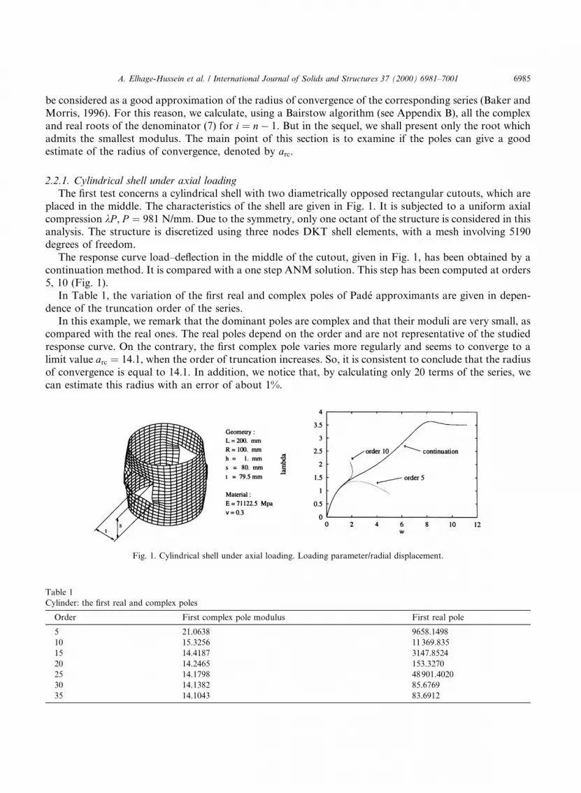
2.2.1. Cylindrical shell under axial loadingThe ®rst test concerns a cylindrical shell with two diametrically opposed rectangular cutouts, which are
placed in the middle. The characteristics of the shell are given in Fig. 1. It is subjected to a uniform axialcompression kP , P � 981 N/mm. Due to the symmetry, only one octant of the structure is considered in thisanalysis. The structure is discretized using three nodes DKT shell elements, with a mesh involving 5190degrees of freedom.
The response curve load±de¯ection in the middle of the cutout, given in Fig. 1, has been obtained by acontinuation method. It is compared with a one step ANM solution. This step has been computed at orders5, 10 (Fig. 1).
In Table 1, the variation of the ®rst real and complex poles of Pad�e approximants are given in depen-dence of the truncation order of the series.
In this example, we remark that the dominant poles are complex and that their moduli are very small, ascompared with the real ones. The real poles depend on the order and are not representative of the studiedresponse curve. On the contrary, the ®rst complex pole varies more regularly and seems to converge to alimit value arc � 14:1, when the order of truncation increases. So, it is consistent to conclude that the radiusof convergence is equal to 14.1. In addition, we notice that, by calculating only 20 terms of the series, wecan estimate this radius with an error of about 1%.
Table 1
Cylinder: the ®rst real and complex poles
Order First complex pole modulus First real pole
5 21.0638 9658.1498
10 15.3256 11369.835
15 14.4187 3147.8524
20 14.2465 153.3270
25 14.1798 48901.4020
30 14.1382 85.6769
35 14.1043 83.6912
Fig. 1. Cylindrical shell under axial loading. Loading parameter/radial displacement.
A. Elhage-Hussein et al. / International Journal of Solids and Structures 37 (2000) 6981±7001 6985

2.2.2. Contact between an elastic beam and a plane rigid surfaceWe consider the contact problem between an elastic beam and a plane rigid surface (Fig. 2). This contact
problem has been solved by the ANM and we refer to Elhage-Hussein et al. (1998) and Elhage-Hussein(1998) for details about the contact algorithm. The line AB contains 26 contact nodes. The structure isdiscretized by 4-node quadrilateral elements with a mesh involving 510 degrees of freedom. The contactforce R at each contact node is regularized by the hyperbolic equation R � g�dÿ h�=h, where h is theclearance, d is the initial clearance, and g is a small regularization parameter. In this test, we have choseg � 10ÿ4.
This contact de®nition admits a singular point at h � 0. So, one can expect that this singularity will leadto a real pole when we use Pad�e approximants.
In Table 2, we present the ®rst real and complex poles with the corresponding truncation orders.For this example, the dominant poles are real. We can also see, as in the case of the cylinder, the ®rst real
pole converges to a limit value arc � 17:06 that we adopt as the radius of convergence.As in the previous example, the ®rst pole with truncation at an order 20 seems to give a good estimate of
the radius of convergence of the series.
2.3. Range of validity of the asymptotic numerical methods representations
In the numerical solution, we do not compute the series, but the truncated series (1) or the rationalapproximation (2). So, we have to de®ne a range of validity of these two approximations, that will be notedrespectively aLS and aLP. These validity limits depend on the truncation order and on the required accuracy.In this section, the series will be truncated at an order 20 and the solution is supposed to be acceptable if theresidual norm is smaller than 10ÿ3.
The evolution of the residual vector along the computed response curves is presented in Appendix C, forthe two previously presented problems.
According to this criterion, the polynomial solution of the cylinder problem is acceptable until a limitvalue aLS � 10:7817 (aLS=arc � 0:7644) of the parameter a, which is then clearly inside the radius of con-
Fig. 2. Contact between an elastic beam and a rigid segment.
Table 2
Contact: the ®rst real and complex poles
Order First complex pole modulus First real pole
5 ± 18.8129
10 ± 17.2527
15 4494.9680 17.0831
20 23.4521 17.0491
25 18.8882 17.0578
30 17.7219 17.0584
35 17.2077 17.0619
6986 A. Elhage-Hussein et al. / International Journal of Solids and Structures 37 (2000) 6981±7001

vergence (Appendix C, Table 1). Concerning the rational solution, the limit of validity is equal toaLP � 16:0179 (aLP=arc � 1:1357) and it is greater than the radius of convergence, given in Section 2.2(Appendix C, Table 2).
With the contact problem, the solution is acceptable until contact at node B takes place, which corre-sponds to the value aLS � 15:6564 (aLS=arc � 0:9176) of the control parameter (Appendix C, Table 3).
For the two examples, the limits of validity of the series are slightly smaller than the radii of convergence,in agreement with the series theory.
2.4. Continuation method based on the series
Because of this limit of validity, the solution path has to be de®ned step by step. Generally within ANM,the end of step criterion and the continuation method are not based on the calculation of the residual, fortwo reasons: First, one tries to avoid the computation of many residual vectors. Second, the residual tendsto increase along the path so that a correction phase would be necessary at each end of step to correctlyinitiate the residual for the next step. To avoid a second matrix inversion per step, one tries to shorten thestep and to have a smaller residual at the end of step (say 10ÿ5±10ÿ4), which permits to choose the newstarting point at the end of the last step: according to the results given in Appendix C, the step shorteningdue to this strategy is rather small. Cochelin has proposed in (Cochelin, 1994) a simple criterion, by requiringthat the di�erence between two successive orders must be smaller than a given accuracy parameter �:
kSn ÿ Snÿ1kkSn ÿ u0k �
kanunkkau1 � � � � � anunk < �: �8�
If one approximates the denominator by the ®rst term, the maximal value is then given by a closed-formexpression for the maximal value ams:
ams � �ku1kkunk
� �1=�nÿ1�: �9�
Such an analysis has been carried out by Cochelin (1994) and various tests have shown that the pathfollowing procedure so-de®ned is e�cient and reliable (Ammar, 1996; Braikat et al., 1997; Cochelin et al.,1994a; Cadou et al., 1998; Elhage-Hussein et al., 1998; Potier-Ferry et al., 1997; Tri et al., 1996; Vannucciet al., 1998; Zahrouni, 1998; Zahrouni et al., 1999; Zahrouni et al., 1998). We recall the pertinent analysisconcerning this criterion in this article for the sake of completeness and compare it with a similar criterionthat we shall introduce for the rational approximation here.
Table 3
Cylinder: evaluation of ams
Order 10 15 20 25 30
� � 10ÿ7 ams 3.7949 6.1656 7.7396 8.8359 9.6426
log10(residual) ÿ6.3220 ÿ6.1337 ÿ6.0250 ÿ5.9009 ÿ5.7642
� � 10ÿ5 ams 6.3302 8.5670 9.8624 10.7049 11.3021
log10(residual) ÿ4.0386 ÿ3.9337 ÿ3.8567 ÿ3.7511 ÿ3.6352
� � 10ÿ3 ams 10.5594 11.9039 12.5673 12.9693 13.2473
log10(residual) ÿ1.7231 ÿ1.7190 ÿ1.6766 ÿ1.5960 ÿ1.5078
A. Elhage-Hussein et al. / International Journal of Solids and Structures 37 (2000) 6981±7001 6987
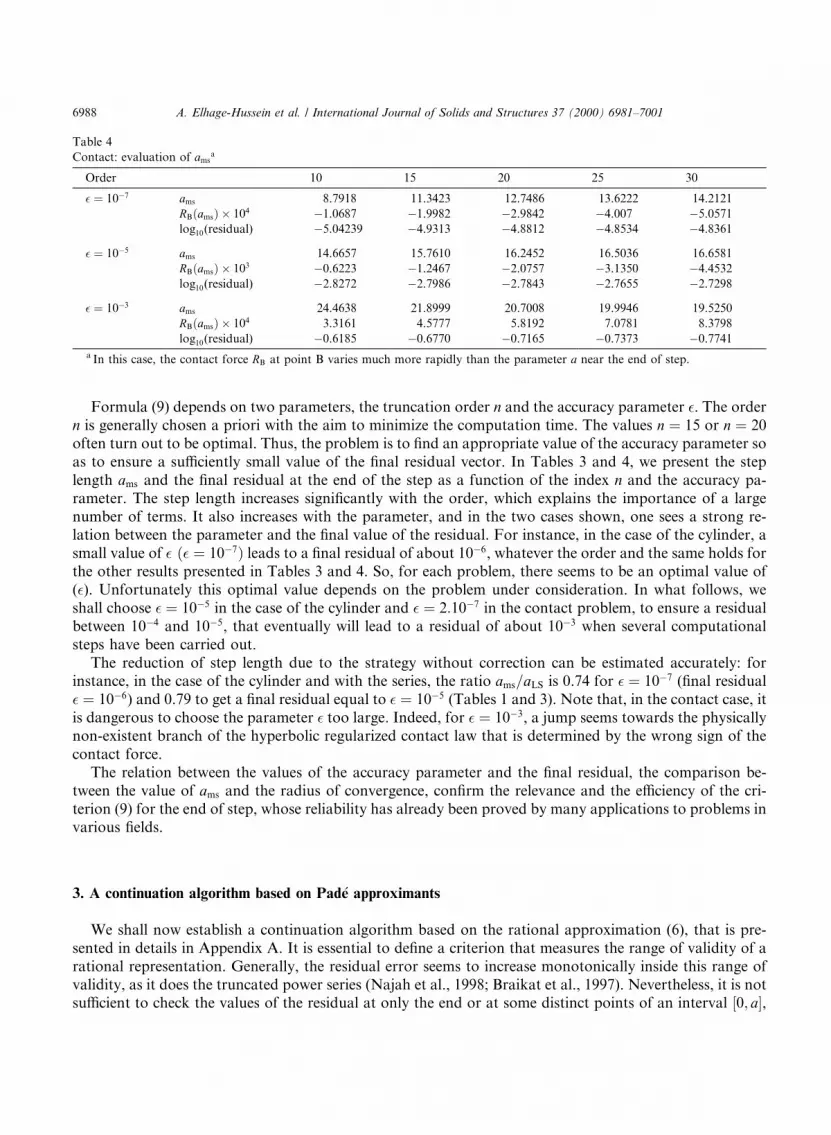
Formula (9) depends on two parameters, the truncation order n and the accuracy parameter �. The ordern is generally chosen a priori with the aim to minimize the computation time. The values n � 15 or n � 20often turn out to be optimal. Thus, the problem is to ®nd an appropriate value of the accuracy parameter soas to ensure a su�ciently small value of the ®nal residual vector. In Tables 3 and 4, we present the steplength ams and the ®nal residual at the end of the step as a function of the index n and the accuracy pa-rameter. The step length increases signi®cantly with the order, which explains the importance of a largenumber of terms. It also increases with the parameter, and in the two cases shown, one sees a strong re-lation between the parameter and the ®nal value of the residual. For instance, in the case of the cylinder, asmall value of � �� � 10ÿ7� leads to a ®nal residual of about 10ÿ6, whatever the order and the same holds forthe other results presented in Tables 3 and 4. So, for each problem, there seems to be an optimal value of(�). Unfortunately this optimal value depends on the problem under consideration. In what follows, weshall choose � � 10ÿ5 in the case of the cylinder and � � 2:10ÿ7 in the contact problem, to ensure a residualbetween 10ÿ4 and 10ÿ5, that eventually will lead to a residual of about 10ÿ3 when several computationalsteps have been carried out.
The reduction of step length due to the strategy without correction can be estimated accurately: forinstance, in the case of the cylinder and with the series, the ratio ams=aLS is 0.74 for � � 10ÿ7 (®nal residual� � 10ÿ6) and 0.79 to get a ®nal residual equal to � � 10ÿ5 (Tables 1 and 3). Note that, in the contact case, itis dangerous to choose the parameter � too large. Indeed, for � � 10ÿ3, a jump seems towards the physicallynon-existent branch of the hyperbolic regularized contact law that is determined by the wrong sign of thecontact force.
The relation between the values of the accuracy parameter and the ®nal residual, the comparison be-tween the value of ams and the radius of convergence, con®rm the relevance and the e�ciency of the cri-terion (9) for the end of step, whose reliability has already been proved by many applications to problems invarious ®elds.
3. A continuation algorithm based on Pad�e approximants
We shall now establish a continuation algorithm based on the rational approximation (6), that is pre-sented in details in Appendix A. It is essential to de®ne a criterion that measures the range of validity of arational representation. Generally, the residual error seems to increase monotonically inside this range ofvalidity, as it does the truncated power series (Najah et al., 1998; Braikat et al., 1997). Nevertheless, it is notsu�cient to check the values of the residual at only the end or at some distinct points of an interval �0; a�,
Table 4
Contact: evaluation of amsa
Order 10 15 20 25 30
� � 10ÿ7 ams 8.7918 11.3423 12.7486 13.6222 14.2121
RB�ams� � 104 ÿ1.0687 ÿ1.9982 ÿ2.9842 ÿ4.007 ÿ5.0571
log10(residual) ÿ5.04239 ÿ4.9313 ÿ4.8812 ÿ4.8534 ÿ4.8361
� � 10ÿ5 ams 14.6657 15.7610 16.2452 16.5036 16.6581
RB�ams� � 103 ÿ0.6223 ÿ1.2467 ÿ2.0757 ÿ3.1350 ÿ4.4532
log10(residual) ÿ2.8272 ÿ2.7986 ÿ2.7843 ÿ2.7655 ÿ2.7298
� � 10ÿ3 ams 24.4638 21.8999 20.7008 19.9946 19.5250
RB�ams� � 104 3.3161 4.5777 5.8192 7.0781 8.3798
log10(residual) ÿ0.6185 ÿ0.6770 ÿ0.7165 ÿ0.7373 ÿ0.7741
a In this case, the contact force RB at point B varies much more rapidly than the parameter a near the end of step.
6988 A. Elhage-Hussein et al. / International Journal of Solids and Structures 37 (2000) 6981±7001

because of the possible occurrence of `defects' in a rational approximation (Baker and Morris, 1996). In-deed, when dealing with Pad�e approximants, the numerator and the denominator of the fractions in Eq. (2)may have roots that are very closely spaced so that the actual function and its approximation are almostequal except in a very small part of the interval. This numerical phenomenon is called a defect of the ra-tional approximation. As a computational code in engineering must be absolutely reliable, these defectsmust be eliminated from the expression of the solution path. To achieve this, we compute all the roots of thecommon denominator Dn of the rational approximation (6) by using a Bairstow algorithm. This algorithmis reiterated in Appendix B. We designate by r, the smallest real root of Dn. If r is smaller than the numberams de®ned by Eq. (9), we give up the rational representation and we go back to the series, at least for thecurrent step. Generally, the smallest root r will be larger than ams. We now try to introduce a criterion forthe value amp of the control parameter, which indicates when the Pad�e approximation (6) is not acceptable.This limit of validity will be sought in the interval [ams; r].
3.1. The criterion to de®ne the step length
According to several trial computations that we conducted, the rational approximations for di�erentorders of truncation yield results that are very close when the parameter a is inside the domain of validity,but beyond this domain they diverge wildly. This is illustrated by Fig. 3, where several rational approxi-mations are pictured for the problem of the cylindrical shell.
Thus, a simple way to achieve our goal seems to extend criterion (9) or (8) to the rational case. In thiscase, one has only to require that the di�erence between two rational solutions at consecutive orders re-mains small at the end of the step. The maximal value amp is then de®ned by
kPn�amp� ÿ Pnÿ1�amp�kkPn�amp� ÿ u0k ' �2; �10�
where �2 is a small number. The number amp in the interval [ams; r] is then sought by the method of bisectionusing criterion (10). This criterion avoids the computation of many residual vectors, which would otherwiseadd to the volume of computations.
Fig. 3. Cylindrical shell: comparison between exact and Pad�e solution with di�erent truncation orders. Loading parameter/radial
displacement.
A. Elhage-Hussein et al. / International Journal of Solids and Structures 37 (2000) 6981±7001 6989

3.2. Some examples with amp computation
We consider the two problems previously described concerning the buckling of cylindrical shell and thecontact problem with a plane obstacle. The so-computed values of the step length: ams for the polynomialapproximation and amp for the one based on Pad�e approximants are presented in Tables 5 and 6.
The accuracy parameters are chosen as �1 � 10ÿ5; �2 � 10ÿ5 ��2 � 2:10ÿ7 in the contact problem) and weconsider various truncation orders 10, 15, 20, 25. With these accuracy parameters, the solution obtained atthe end of step is better than the rational approximation. Nevertheless, the Pad�e approximants increase thedomain of validity. This improvement does not appear to be as important as in the contact case, but re-member that the value of the contact force is more relevant than the path parameter to evaluate the part ofthe solution branch that has been accounted for.
Note that the Pad�e approximants are calculated by a simple Gram±Schmidt orthogonalization proce-dure (Appendix A) which adds only little in computing time as compared with the computation of theseries.
3.2.1. Other examplesIn this example, we consider a curved shell hinged along two opposite sides, which is submitted to a
concentrated force at the central point (Fig. 4). Assuming symmetry conditions, only one quarter of theshell is studied and discretized with 200 shell elements of DKT type.
The analysis is carried out with two di�erent values of the thicknesses h1 � 6:35 mm and h2 � 12:7 mm.The truncation order has been ®xed at 20. Figs. 5 and 6, describe the ®rst solution step obtained by theseries and the Pad�e approximants using accuracy parameters �1 � �2 � 10ÿ5.
With the thick shell, criterion (9) gives a limit value ams � 67:21, which corresponds to a de¯ectionw � 12:04 mm. With criterion (10), the range of validity of the Pad�e representation is approximatelyamp � 82:09, which corresponds to w � 13:83 mm. The modulus of the ®rst complex pole is arc � 88.52.
Table 5
Cylinder: the quality of the series and of the Pad�e solution at the end of the ®rst step with the two displacement criteria
Order Series Pad�e
ams log10(residual) amp log10(residual)
10 6.3302 ÿ4.0386 7.7173 ÿ4.0769
15 8.5670 ÿ3.9336 11.6327 ÿ4.2902
20 9.8623 ÿ3.8568 14.3456 ÿ3.8822
25 10.7049 ÿ3.7511 16.6730 ÿ4.2302
30 11.3021 ÿ3.6352 18.2748 ÿ4.6459
Table 6
Contact: the quality of the series and of the Pad�e solution at the end of the ®rst step with the two displacement criteria. R is the contact
force at node B with g � 10ÿ4
Order Series Pad�e
ams RB�ams� � 103 log10(residual) amp RB�amp� � 103 log10(residual)
10 14.6657 ÿ0.6223 ÿ3.5793 14.9890 ÿ0.7365 ÿ5.3619
15 15.7610 ÿ1.2467 ÿ3.5438 16.0916 ÿ1.7163 ÿ5.3659
20 16.2452 ÿ2.0757 ÿ3.5297 16.4461 ÿ2.8018 ÿ5.4585
25 16.5036 ÿ3.1350 ÿ3.3079 16.5729 ÿ3.5819 ÿ5.3374
30 16.6581 ÿ4.4532 ÿ3.06284 16.7582 ÿ5.9054 ÿ4.5612
6990 A. Elhage-Hussein et al. / International Journal of Solids and Structures 37 (2000) 6981±7001

Fig. 4. Elastic cylindrical shell loaded by a concentrated force.
Fig. 5. Thick shell: loading parameter/displacement of the central point, validity limit of the polynomial and the rational solution.
Fig. 6. Thin shell: loading parameter/displacement of the central point, validity limit of the polynomial and the rational solution.
A. Elhage-Hussein et al. / International Journal of Solids and Structures 37 (2000) 6981±7001 6991

Therefore, in this case the range of validity of the rational approximation does not extend to the radius ofconvergence.
The extension of the step length seems to be more important with the thin shell example. The validitybounds for the two representations are ams � 21.98 and amp� 48.32 corresponding to w � 6:01 andw � 11:87, respectively. The modulus of the ®rst complex pole is arc � 30:14, so that the range of validity ofthe rational approximation extends much beyond the radius of convergence.
3.3. Continuation algorithm
In this section, we propose the continuation algorithm based on the rational representation. It can besummarized as follows:(1) Computation of the asymptotic solution:
± Compute the series until a given order n.± Calculate the validity limit ams of the polynomial solution by the displacement criterion (9)
(2) Computation of the simultaneous Pad�e approximants (see Appendix A)± Gram±Schmidt orthogonalization procedure.± Computation of the denominator Dnÿ1.
(3) Choice of the solution:± Solving Dnÿ1 � 0 by the Bairstow algorithm (see Appendix B), the ®rst real root is designed by r.± If jrj < jamsj, we consider the polynomial solution:
Sn�u�a��; a 2 �0; ams�;Sn�k�a��:
�± If jrj > jamsj, calculate amp, satisfying criterion (10), in the interval [ams; r], and form the Pad�e ap-
proximant solution:
Pn�u�a��; a 2 �0; amp�;Pn�k�a��:
�(4) Rede®ne a new starting point for the next step which corresponds to the end of step obtained at (3) for
a � ams or a � amp and go back to (1).
4. Applications of the continuation algorithm
In this section, we consider various numerical examples in order to discuss and validate the algorithmpresented in Section 3: the previously described problems of the shallow shells under concentrated loadsand the one of the cylindrical shell, the contact problem and the classical buckling problem of an archinvolving two bifurcating branches. In all the cases, the series are truncated at the order 20. In these cal-culations, the total step number is the measure of e�ciency of the algorithm and the rational approximationwill be compared with the polynomial one and sometimes with classical iterative methods.
4.1. Shallow shells loaded by a concentrated force
First, we considered the two curved shell problems (Fig. 4), whose ®rst computational step has just beenanalyzed and we applied the continuation methods till the de¯ection reaches the value w � 30:5 mm. Withthe rational approximation, this solution path requires only two steps for the thick shell and seven stepswith the thin shell, whereas the same computation requires, respectively, four and 12 steps with using the
6992 A. Elhage-Hussein et al. / International Journal of Solids and Structures 37 (2000) 6981±7001
series expansion. So, it appears that the use of the Pad�e approximants leads to a reduction of the com-putational steps by a factor of about two.
These classical benchmarks had been previously considered in many articles, for instance, in Ammar(1996) and Simo et al. (1990). According to the ®rst author, the most rapid iterative method is the modi®edNewton method, that yields the curve of Fig. 5 in 30 steps, i.e. 30 matrix decompositions, but as usually, themethod is not reliable and diverges if one prescribes a larger step. As for the Newton±Raphson method,most of authors solve the thick shell problem in at least 10 steps and the thin one in at least 15 steps, withabout three iterations per step. This results in 40±70 matrix decompositions in the ®rst case, 60±100 in thesecond one. In terms of computation time, one can consider that one step with the ANM is equivalent totwo matrix decompositions (Cochelin et al., 1994a; Zahrouni et al., 1999, 1998), so that the computationtime within the present method is equivalent to four and 14 matrix decompositions within Newton±Raphson algorithms: this is an illustration of the e�ciency of the presented continuation method, ascompared with classical incremental-iterative algorithms. Remark also that it does not seem possible todescribe the two response curves with less than 10 and 15 points: this type of requirement limits the e�-ciency of classical methods as much as problems of convergence.
4.2. Cylindrical shell
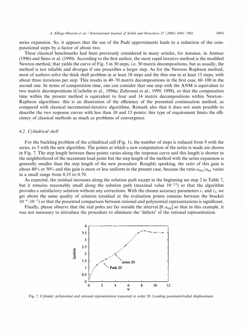
For the buckling problem of the cylindrical cell (Fig. 1), the number of steps is reduced from 9 with theseries, to 5 with the new algorithm. The points at which a new computation of the series is made are shownin Fig. 7. The step length between these points varies along the response curve and this length is shorter inthe neighborhood of the maximum load point but the step length of the method with the series expansion isgenerally smaller than the step length of the new procedure. Roughly speaking, the ratio of this gain isabout 40% or 50% and this gain is more or less uniform in the present case, because the ratio amp=ams variesin a small range from 0.35 to 0.70.
As expected, the residual increases along the solution path except in the beginning see step 2 in Table 7,but it remains reasonably small along the solution path (maximal value 10ÿ2:8) so that the algorithmprovides a satisfactory solution without any corrections. With the chosen accuracy parameters �1 and �2, weget about the same quality of solution (residual at the evaluation points remains between the bracket10ÿ4±10ÿ3) so that the presented comparison between rational and polynomial representations is signi®cant.
Finally, please observe that the real poles are far outside the interval [0; amp] so that in this example, itwas not necessary to introduce the procedure to eliminate the `defects' of the rational representation.
Fig. 7. Cylinder: polynomial and rational representation truncated at order 20. Loading parameter/radial displacement.
A. Elhage-Hussein et al. / International Journal of Solids and Structures 37 (2000) 6981±7001 6993

4.3. Buckling of a circular arch
We consider a deep circular arch submitted to a vertical force applied at the center and to a perturbationforce P � F =100 placed excentrally (Fig. 8). To analyze this classical benchmark problem, we used the samesoftware as in the previous examples, that is based on the DKT shell element, which is based on theframework of small moderate rotations. Of course, that framework is not perfectly adapted to the case of adeep shell but the equilibrium path (Fig. 9) has qualitatively the same features as the deep shell model.There are two quasi-bifurcations in this response curve: that is why this example is a severe test for thereliability of a path following technique. As this is a quasi-bifurcation problem, the computations cannot be
Table 7
Continuation algorithm with rational representation, �1 � �2 � 10ÿ5
Step ams amp First real pole log10(residual)
1 9.8623 14.3455 153.3270 ÿ3.8821
2 7.7721 22.0473 53.4529 ÿ3.9564
3 20.7197 29.4371 90.4589 ÿ2.9707
4 10.7401 22.7509 74.7979 ÿ2.8213
5 ÿ18.3048 ÿ26.4700 ÿ83.6267 ÿ2.8010
Fig. 8. Arch: 200 elements DKT mesh, 1212 dof.
Fig. 9. Equilibrium path: loading parameter/displacement at the middle of the arch.
6994 A. Elhage-Hussein et al. / International Journal of Solids and Structures 37 (2000) 6981±7001

carried out without choosing very small values for the accuracy parameters (�1 � 10ÿ14 and �2 � 10ÿ9). As aconsequence, the residual remains very small along the computed path and no iterative corrections areneeded. With the series representation, 200 solution steps are necessary to obtain the solution path, whichreduces to 39 with the Pad�e representation. These large numbers of steps are due to the large curvature ofthe path close to the bifurcation points: for instance, one is close to the ®rst bifurcation point from step 2 tostep 10, to the second one from step 15 to step 20 and again close to the ®rst one from steps 30 to 39 (Table8). As in the previous example, the ratio ams=amp is generally in the range 0.35±0.75 so that the rationalapproximation should reduce the number of steps by a factor of about two. In actual run, the number ofsteps is reduced by a factor of ®ve, which is due to very large ratios amp=ams for a few steps (steps 10 and 25).
In one case (step 11), we found a real pole in the interval [0; ams], and according to the algorithm, the 11thstep is carried out with the series representation. This establishes that the computation of the poles is ef-fective and improves the robustness of the algorithm. In another case (step 3), the step length amp and thesmallest real pole lie very close together, what implies that one can get a very accurate solution up to thepole: this phenomenon is typical of a `defect' in a Pad�e approximant and it shows that it is not su�cient tocheck only some values of the residual in order to ensure the resolution of the solution path in a giveninterval.
This example shows that the Pad�e algorithm combines e�ciency and robustness. Indeed, it reduced thenumber of steps with respect to the series with a factor of ®ve and it permitted to compute this intricateequilibrium path without any di�culty. The analysis also shows the importance of the control of the polesof the rational representation in the formulation of the algorithm.
This example has been designed to be a severe test for a path following technique, especially thesmallness of the force ratio P=F . We have tried to achieve this computation by the standard algorithms ofthe commercial code ABAQUS, but the algorithms have diverged. Likely the most e�cient would be toapply a procedure speci®c for bifurcation problems, see for instance, Vannucci et al. (1998), but here theaim is to discuss generic path following technique.
4.4. Contact between a 2-D elastic beam and a plane rigid surface
We now return to the contact previously described (Fig. 2). The accuracy parameters are chosen as givenin Table 9 together with the particulars of the computation. To obtain the solution path up to k � 1, 90steps are needed with the series expansion but only 51 steps with the rational representation. Compared tothis result the engineering code (ABAQUS) requires the factoring of 128 sti�ness matrices. The residuals in
Table 8
Pad�e continuation algorithm with truncation at order 20: �1 � 10ÿ14, �2 � 10ÿ9
Step ams amp First real pole W log10(Pad�e residual)
1 496.7623 766.0646 1035.3670 5.3821 ÿ7.5602
2 190.5040 252.4374 261.2850 9.6583 ÿ8.0901
3 6.7843 8.8822 8.8843 9.8741 ÿ8.0967
4 0.001002 0.001512 0.00236 9.8742 ÿ8.0959
5 0.00113 0.00228 0.00296 9.9077 ÿ8.0952
10 ÿ0.6326 ÿ10.2266 ÿ62.0343 10.0243 ÿ6.2804
11 ÿ12.3055 ± ÿ9.0793 37.5081 ÿ6.2799
15 ÿ112.5832 ÿ313.3450 ÿ380.2656 123.3377 ÿ5.7953
20 ÿ16.1427 ÿ27.0950 ÿ31.3806 122.4159 ÿ4.9616
25 ÿ2.6802 ÿ66.2319 ÿ511.0942 88.7651 ÿ4.7605
30 87.8300 216.1468 2140.8985 22.5629 ÿ4.6465
39 ÿ46.8303 ÿ73.7248 ÿ89.8615 10.2850 ÿ5.0552
A. Elhage-Hussein et al. / International Journal of Solids and Structures 37 (2000) 6981±7001 6995

our procedure remain relatively small although we could have obtained a high accuracy if we had intro-duced some corrector iterations after step 25. As in the previous case, some of the steps (5, 25, 51) seem tohave played an important part in the improvement of the calculation by the rational approximation. In atleast four cases, the necessity to control the poles of the rational approximation is manifest: in step 32,where a real pole is detected in the range of validity of the series and in step 4, 40 and 45, where the steplength amp is almost equal to the ®rst real pole.
5. Conclusion
In this article, we proposed a new variant of a continuation algorithm based on Pad�e approximants anddemonstrated the e�ciency and the robustness of the method. Roughly speaking, the method is capable toreduce the number of steps by a factor of two as compared to the same method based on series expansion;in one case this fact was even ®ve. In principle, the rational representation is less stable than the polynomialone. That is why, as a precaution, we introduced a new step length criterion. The numerical tests that wecarried out show that this criterion cannot be omitted. As far as the reliability of the algorithm is concerned,it never failed in the ®ve examples that we studied here inspite of the fact that these examples involve limitpoints, quasi-bifurcations and unilateral contact.
Incidentally, the expectation that the knowledge of the poles permits one to estimate the radii of con-vergence of the series is con®rmed by these calculations.
According to several recent studies (Ammar, 1996; Cochelin, 1994; Cadou et al., 1998; Zahrouni et al.,1999), the representation by series leads to continuation method, which is more e�cient than the classicalincremental-iterative method. The method that we proposed here can reduce by half the computationaltime with respect to the series method. It is likely that the present method is not really the best possiblevariant in the class of asymptotic numerical algorithms because, we considered only a type of Pad�e ap-proximant among the many possibilities (Baker and Morris, 1996; Brezinski and Iseghem, 1994) that exist.The reduced basis algorithms (Lewandowski, 1987; Noor, 1981; Noor and Peters, 1980, 1981) could also bemodi®ed with a view to diminish their computational time.
Table 9
Pad�e continuation algorithm with truncature at order 20: �1 � 10ÿ5; �2 � 2:10ÿ7
Step ams amp amp=ams First real pole log10(Pad�e residual)
1 16.2451 16.4461 1.01 17.0490 ÿ5.6355
2 0.552861 0.552869 1.00 0.6789 ÿ4.5939
3 0.0950 0.1410 1.48 0.1563 ÿ4.6296
4 0.1364 0.25537140 1.87 0.255385 ÿ4.6223
5 0.3106 2.0742 6.67 5.0135 ÿ4.2449
10 0.1753 0.2435 1.38 2.3579 ÿ3.9892
15 0.1125 0.1499 1.33 0.1624 ÿ3.5283
20 0.0650 0.1495 2.29 0.4028 ÿ3.0608
25 0.0421 0.1461 3.46 0.3193 ÿ2.9851
30 0.0983 0.1153 1.17 277.8555 ÿ2.7010
32 0.1054 ± ± 0.06634 ÿ2.4639
35 0.0901 0.1163 1.29 0.2995 ÿ2.5477
40 0.0129 0.0206 1.58 0.0206 ÿ2.6758
45 0.01003 0.0158 1.57 0.01619 ÿ2.8206
51 0.0733 0.2538 3.46 0.7953 ÿ3.1915
6996 A. Elhage-Hussein et al. / International Journal of Solids and Structures 37 (2000) 6981±7001

Acknowledgements
This article is dedicated to Prof. W.T. Koiter, who was the author of many decisive contributions invarious ®elds. In elastic stability, he was 20 years ahead of the engineering community and 25 years aheadof the mathematicians working on bifurcation theory. One of us (Michel Potier-Ferry) has often interactedwith him and keeps a delightfull memory of his simplicity and his sharp scienti®c views.
Appendix A. Pad�e approximants for series of vector
Since H. Pad�e's Thesis, 1892, we know that rational fractions are more appropriate than polynomials torepresent a function. One can ®nd a modern presentation of Pad�e approximant in Baker and Morris (1996).We use Pad�e approximants in the ANM in the following manner:
(1) From the vectors U1;U2; . . . ;Up, we build up an orthogonal basis by the classical Gram±Schmidtprocedure (We detail the computations for p � 6):
U1 � a11U�1;U2 � a21U�1 � a22U�2;U3 � a31U�1 � a32U�2 � a33U�3;U4 � a41U�1 � a42U�2 � a43U�3 � a44U�4;U5 � a51U�1 � a52U�2 � a53U�3 � a54U�4 � a55U�5;U6 � a61U�1 � a62U�2 � a63U�3 � a64U�4 � a65U�6 � a66U�6:
8>>>>>><>>>>>>:Then, we introduce this into the polynomial representation, which introduces six polynomials with a de-creasing degree (from 5 to 0) as factors of the vector ®elds Uk
UÿU0 � aU�1�a11 � aa21 � a2a31 � a3a41 � a4a51 � a5a61� � a2U�2�a22 � aa32 � a2a42 � a3a52 � a4a62�� a3U�3�a33 � aa43 � a2a53 � a3a63� � a4U�4�a44 � aa54 � a2a64� � a5U�5�a55 � aa65�� a6U�6�a66�:
(2) We replace the polynomials by Pad�e approximants having the same denominator (D5 � d1�ad2 � � � � � a5d5), in the following way:
a11 � aa21 � a2a31 � a3a41 � a4a51 � a5a61 � b0�ab1�a2b2�a3b3�a4b4
D5;
a22 � aa32 � a2a42 � a3a52 � a4a62 � c0�ac1�a2c2�a3c3
D5;
a33 � aa43 � a2a53 � a3a63 � e0�ae1�a2e2
D5;
a44 � aa54 � a2a64 � f0�af1
D5;
a55 � aa65 � g0
D5:
8>>>>>><>>>>>>:The coe�cients bi, ci, ei, fi and gi are computed by the same principles as with the classical Pad�e ap-proximants; we require that each fraction has the same Taylor expansions as the corresponding polyno-mials up to order 5, 4, 3, 2, 1, respectively. This results:
b0 � a11;b1 � a21 � a11d1;b2 � a31 � a21d1 � a11d2;b3 � a41 � a31d1 � a21d2 � a11d3;b4 � a51 � a41d1 � a31d2 � a21d3 � a11d4;
A. Elhage-Hussein et al. / International Journal of Solids and Structures 37 (2000) 6981±7001 6997

c0 � a22; e1 � a43 � a33d1;c1 � a32 � a22d1; e2 � a53 � a43d1 � a33d2;c2 � a42 � a32d1 � a22d2; f0 � a44;c3 � a52 � a42d1 � a32d2 � a22d3; f1 � a54 � a44d1;e0 � a33; g0 � a55;
and the coe�cients of D5 � d1 � ad2 � � � � � a5d5 are solutions of the triangular system
a61 � a51d1 � a41d2 � a31d3 � a21d4 � a11d5 � 0;a62 � a52d1 � a42d2 � a32d3 � a22d4 � 0;a63 � a53d1 � a43d2 � a33d3 � 0;a64 � a54d1 � a44d2 � 0;a65 � a55d1 � 0:
8>>>><>>>>:(3) After some rearrangements, we arrive at a new form of the previous rational representation, that
involves only vectors Uk and the coe�cients di
UÿU0 � aD4
D5
U1 � a2 D3
D5
U2 � a3 D2
D5
U3 � a4 D1
D5
U4 � a5 1
D5
U5:
We do the same for the control parameter
kÿ k0 � aD4
D5
k1 � a2 D3
D5
k2 � a3 D2
D5
k3 � a4 D1
D5
k4 � a5 1
D5
k5:
Appendix B. Bairstow's algorithm
The principle of this technique is to compute, two by two, the roots of a polynomial Dn�a� � 0 �n P 2�.The algorithm is described in what follows:
(1) As Dn�a� admits at least two real or complex roots, it can be written as a product of a polynomialQ�a� and a polynomial of second degree a2 ÿ sa� p, where s and p are, respectively the sum and theproduct of the two of roots.
The Euclidian division of Pn�a� by (a2 ÿ sa� p) leads to the equation:
Dn�a� � �a2 ÿ sa� p�Q�a� � R�a�; �B:1�
where
Q�a� � qnanÿ2 � qnÿ1anÿ3 � � � � � q3a� q2;R�a� � q1a� q0:
�The coe�cients q1 and q0 depend on s and p. The sought values of s and p are the values producing a zero ofthe polynomial R�a�. s and p are then solutions of the following non-linear system:
q0�s; p� � 0;q1�s; p� � 0:
��B:2�
Coe�cients of the polynomials Q and R are obtained by identifying the powers of �a� in Eq. (B.1):
6998 A. Elhage-Hussein et al. / International Journal of Solids and Structures 37 (2000) 6981±7001

qn � dn;qnÿ1 � dnÿ1 � sqn;qk � dk � sqk�1 ÿ pqk�2; 1 6 k 6 �nÿ 2�;q0 � d0 ÿ pq2:
8>><>>: �B:3�
Table 10
Cylinder: the loading parameter and the quality of the polynomial approximation, truncated at order 20, with respect to the parameter a
a=arc �arc � 14:1� k log10(residual)
0.1006 0.2179 ÿ11.9749
0.2012 0.4223 ÿ11.9303
0.3018 0.6122 ÿ11.3110
0.4023 0.7862 ÿ8.7807
0.5030 0.9431 ÿ6.8014
0.6035 1.0820 ÿ5.1758
0.7041 1.2030 ÿ3.7950
0.7644 1.2674 ÿ3.0559
0.8047 1.3075 ÿ2.5944
0.9052 1.3997 ÿ1.5341
1.0059 1.4940 ÿ0.5904
Table 12
Contact: the contact force, the clearance h and the quality of the polynomial approximation, truncated at order 20, with respect to the
parameter a
a=arc �arc � 17:06� RB � 103 hB log10(residual)
0.1370 ÿ0.0159 1.7253 ÿ9.9236
0.2739 ÿ0.0379 1.4507 ÿ9.8789
0.4109 ÿ0.0701 1.1761 ÿ9.8173
0.5478 ÿ0.1218 0.9015 ÿ7.5735
0.6848 ÿ0.2189 0.6270 ÿ5.6373
0.8217 ÿ0.4672 0.3526 ÿ4.0576
0.9176 ÿ1.1434 0.1608 ÿ3.1046
0.9587 ÿ2.4390 0.0788 ÿ2.7229
0.9724 ÿ3.7854 0.0514 ÿ2.5877
0.9861 ÿ8.1696 0.0241 ÿ2.3858
Table 11
Cylinder: the loading parameter and the quality of the rational approximation, truncated at order 20, with respect to the parameter a
a=arc �arc � 14:1� k log10(residual)
0.1622 0.3448 ÿ11.9435
0.3245 0.6529 ÿ11.9087
0.4867 0.9190 ÿ10.8543
0.6489 1.1388 ÿ8.0757
0.8112 1.3135 ÿ5.9032
0.9734 1.4525 ÿ4.2451
1.1357 1.5703 ÿ3.0547
1.2980 1.6786 ÿ2.2313
1.4601 1.7842 ÿ1.6580
1.6223 1.8907 ÿ1.2360
A. Elhage-Hussein et al. / International Journal of Solids and Structures 37 (2000) 6981±7001 6999

By calculating the derivative (B.3) with respect to s and p, we obtain the following equations:
oqnos � 0;oqnÿ1
os � qn;oqkos � qk�1 � s oqk�1
os ÿ p oqk�2
os ; 1 6 k 6 �nÿ 2�;oq0
os � ÿp oq2
os :
8>>><>>>:oqnop � 0;oqnÿ1
op � s oqnop ;
oqkos � s oqk�1
op ÿ qk�2 ÿ p oqk�2
op ; 1 6 k 6 �nÿ 2�;oq0
op � ÿq2 ÿ p oq2
op :
8>>>><>>>>:(2) We get the values of s and p by applying an iterative Newton method to the system (B.2).(3) We deduce the coe�cients of the polynomial Q�a�, and go back to step (1) as long as necessary to
calculate all the roots.
Appendix C
For the sake of completeness, we present in detail the evolution of the residual along a step in typicalcases discussed in Section 2. By comparison of Tables 10 and 11, it appears that the rational approximationimproves the quality of the solution along the whole step. According to these tables, the requirement of aresidual of 10ÿ5 instead of 10ÿ3 induces a small shortening of the step of about 20% or 30%: this illustratesthe interest of a strategy without correction (Table 12).
References
Almroth, B.O., Brogan, F.A., Stern, P., 1978. Automatic choice of global shape functions in structural analysis. AIAA 16, 525±528.
Ammar, S., 1996. M�ethode asymptotique num�erique perturb�ee appliqu�ee �a la r�esolution des probl�emes non lin�eaires en grande
rotation et grand d�eplacement. Thesis, Universit�e Laval Qu�ebec, Facult�e des sciences et de g�enie.
Azrar, L., Cochelin, B., Damil, N., Potier-Ferry, M., 1992. An asymptotic-numerical method to compute bifurcating branches. In:
Ladv�eze, P., Zienkiewicz, O.C. (Eds.), New Advances in Computational Structural Mechanics. Elsevier, Amsterdam, pp. 117±131.
Baker, G.A., Morris, P.G., Basic Theory, Encyclopedia of Mathematics and its Applications, vol. 13 1996 Addison-Wesley New York.
Boutyour, E.H., Cochelin, B., Potier-Ferry, M., 1993. Calcul des points de bifurcation par une m�ethode asymptotique num�erique. I
Congr�es National de M�ecanique au Maroc, pp. 371±378.
Braikat, B., Damil, N., Potier-Ferry, M., 1997. M�ethode asymptotique num�erique pour la plasticit�e. Revue Europ�eenne des �El�ements
Finis 6 (3), 337±357.
Brezinski, C., Iseghem, V., 1994. Pad�e approximants. In: Ciarlet, P.G., Lions, J.L. (Eds.), Handbook of Numerical Analysis, vol. 3.
North-Holland, Amsterdam.
Brunelot, J., 1999. Simulation de la mise en forme �a chaud par la m�ethode asymptotique num�erique. Thesis, Universit�e de Metz.
Cadou, J.M., Cochelin, B., Damil, N., Potier-Ferry, M., 2000. Asymptotic numerical method for strongly non-linear problems:
application to stationary Navier±Stokes equation and Petrov±Galerkin formulation. International Journal for Numerical Methods
in Engineering, submitted for publication.
Cochelin, B., 1994. A path-following technique via an asymptotic-numerical method. Computers and Structures 53 (5), 1181±1192.
Cochelin, B., Damil, N., Potier-Ferry, M., 1994a. The asymptotic-numerical method: an e�cient perturbation technique for non-linear
structural mechanics. Revue Europ�eenne des El�ements Finis 3 (2), 281±297.
Cochelin, B., Damil, N., Potier-Ferry, M., 1994b. Asymptotic numerical methods and Pad�e approximants for non linear elastic
structures. International Journal for Numerical Methods in Engineering 37, 1187±1213.
de Boer, H., van Keulen, F., 1997. Pad�e approximants applied to a non-linear ®nite element solution strategy. Communications in
Numerical Methods in Engineering 13, 593±602.
7000 A. Elhage-Hussein et al. / International Journal of Solids and Structures 37 (2000) 6981±7001

Elhage-Hussein, A., 1998. Mod�elisation des probl�emes de contact par une m�ethode asymptotique num�erique. Thesis, Universit�e de
Metz.
Elhage-Hussein, A., Damil, N., Potier-Ferry, M., 1998. An asymptotic numerical algorithm for frictionless contact problems. Revue
Europ�eenne des �El�ements Finis 7 (1±3), 119±130.
Kawahara, M., Yoshimura, N., Nakagawa, K., Ohsaka, H., 1976. Steady and unsteady ®nite element analysis of incompressible
viscous ¯uid. International Journal for Numerical Methods in Engineering 10, 437±456.
Lewandowski, R., 1987. Application of the Ritz method to the analysis of non-linear free vibrations of beams. Journal of Sound and
Vibration 114 (1), 91±101.
Najah, A., Cochelin, B., Damil, N., Potier-Ferry, M., 1998. A critical review of asymptotic numerical methods. Archives of
Computational Methods in Engineering 5 (1), 31±50.
Noor, A.K., 1981. Recent advances in reduction methods for non-linear problems. Computers and Structures 13, 31±44.
Noor, A.K., Peters, J.M., 1980. Reduced basis technique for non-linear analysis of structures. AIAA Journal 18 (4) 79±0747R, 1980.
Noor, A.K., Peters, J.M., 1981. Tracing post-limit-point paths with reduced basis technique. Computer Methods in Applied Mechanics
and Engineering 28, 217±240.
Pad�e, H., 1892. Sur la repr�esentation approach�ee d'une fonction par des fractions rationnelles. Annales de l'Ecole Normale Sup. 9 (3),
3±93.
Potier-Ferry, M., Cao, H.L., Brunelot, J., Damil, N., 2000. An asymptotic numerical method for numerical analysis of large
deformation viscoplastic problems. Computers and Structures, in press.
Potier-Ferry, M., Damil, N., Braikat, B., Brunelot, J., Cadou, J.M., Cao, H., Elhage-Hussein, A., 1997. Traitement des fortes non-
lin�earit�es par la m�ethode asymptotique num�erique. Comptes Rendus de l'Acad�emie des Sciences t. 324 serie IIb, 171±177.
Simo, J.C., Fox, D.D., Rifai, M.S., 1990. On a stress resultant geometrically exact shell model, part III: computational aspects of the
non-linear theory. Computer Methods in Applied Mechanics and Engineering 79, 21±70.
Thompson, J.M.T., Walker, A.C., 1968. The non-linear perturbation analysis of discrete structural systems. International Journal of
Solids and Structures 4, 757±768.
Tri, A., Cochelin, B., Potier-Ferry, M., 1996. R�esolution des �equations de Navier±Stokes et d�etection des bifurcations stationnaires par
une m�ethode asymptotique num�erique. Revue Europ�eenne des �El�ements Finis 5 (4), 415±442.
Van-Dyke, M., 1984. Computed-extended series. Annual Review in Fluid Mechanics 16, 287±309.
Vannucci, P., Cochelin, B., Damil, N., Potier-Ferry, M., 1998. An asymptotic numerical method to compute bifurcating branches.
International Journal for Numerical Methods in Engineering 41, 1365±1389.
Zahrouni, H., 1998. M�ethode asymptotique num�erique pour les coques en grandes rotations. Thesis, Universit�e de Metz.
Zahrouni, H., Cochelin, B., Potier-Ferry, M., 1999. Computing ®nite rotations of shells by an asymptotic-numerical method.
Computer Methods in Applied Mechanics and Engineering, 175, 71±85.
Zahrouni, H., Potier-Ferry, M., Elasmar, H., Damil, N., 1998. Asymptotic numerical method for non-linear constitutive laws. Revue
Europ�eenne des �El�ements Finis, 7, 841±869.
A. Elhage-Hussein et al. / International Journal of Solids and Structures 37 (2000) 6981±7001 7001