productivity, welfare and reallocation
TRANSCRIPT

Policy Research Working Paper 5226
Productivity, Welfare and Reallocation
Theory and Firm-Level Evidence
Susanto BasuLuigi Pascali
Fabio SchiantarelliLuis Serven
The World BankDevelopment Research GroupMacroeconomics and Growth TeamMarch 2010
WPS5226P
ublic
Dis
clos
ure
Aut
horiz
edP
ublic
Dis
clos
ure
Aut
horiz
edP
ublic
Dis
clos
ure
Aut
horiz
edP
ublic
Dis
clos
ure
Aut
horiz
ed

Produced by the Research Support Team
Abstract
The Policy Research Working Paper Series disseminates the findings of work in progress to encourage the exchange of ideas about development issues. An objective of the series is to get the findings out quickly, even if the presentations are less than fully polished. The papers carry the names of the authors and should be cited accordingly. The findings, interpretations, and conclusions expressed in this paper are entirely those of the authors. They do not necessarily represent the views of the International Bank for Reconstruction and Development/World Bank and its affiliated organizations, or those of the Executive Directors of the World Bank or the governments they represent.
Policy Research Working Paper 5226
A considerable literature has focused on the determinants of total factor productivity (TFP), prompted by the empirical finding that TFP accounts for the bulk of long-term growth. This paper offers a deeper reason for such focus: the welfare of a representative consumer is summarized by current and anticipated future Solow productivity residuals. The equivalence holds for any specification of technology and market structure, as long as the representative household maximizes utility while taking prices parametrically. This result justifies total factor productivity as the right summary measure of welfare, even in situations where it does not properly measure technology, and makes it possible to calculate the contributions of disaggregated units (industries or
This paper—a product of the Macroeconomics and Growth Team, Development Research Group—is part of a larger effort in the department to assess the determinants of productivity and growth. Policy Research Working Papers are also posted on the Web at http://econ.worldbank.org. The author may be contacted at [email protected].
firms) to aggregate welfare using readily available data. Based on this finding, the authors compute firm and industry contributions to welfare for a set of European countries (Belgium, France, Great Britain, Italy, Spain) using industry-level and firm-level data. With additional assumptions about technology and market structure (specifically, that firms minimize costs and face common factor prices), the authors show that welfare change can be further decomposed into three components that reflect, respectively, technical change, aggregate distortions, and allocative efficiency. Then, using the appropriate firm-level data, they assess the importance of each of these components as sources of welfare improvement in the same set of European countries.

Productivity, Welfare and Reallocation:
Theory and Firm-Level Evidence�
Susanto BasuBoston College and NBER
Luigi PascaliBoston College
Fabio SchiantarelliBoston College and IZA
Luis Serveny
World Bank
March 1, 2010
JEL: D24, D90, E20, O47Keywords: Productivity, Welfare, Reallocation, Technology, TFP
�We would like to thank John Haltiwanger, Chad Syverson and the participants at the NBER Summer Institute,NBER Productivity Lunch, Ottawa Productivity Workshop and Bocconi University seminar for helpful discussionsand suggestions.
yBasu: [email protected]; Pascali: [email protected]; Schiantarelli: [email protected]; Serven:[email protected]
1
1 Introduction
How much of growth comes from innovation and technical advances, and how much from changes in
allocative e¢ ciency? This question arises in a variety of contexts, in �elds as diverse as growth and
development, trade, and industrial organization. Yet, despite the importance of the question, there
is no consensus regarding the answer. A large number of papers have proposed a bewildering variety
of methods to measure the importance of allocative e¢ ciency, leading to a wide range of numerical
estimates. Much of the confusion is due to the lack of an organizing conceptual framework for
studying this issue. We propose such a framework, and then provide a quantitative answer using
one particular set of data.
In starting such a project, one immediately faces the question: What do we mean by allocative
e¢ ciency? Indeed, what do we mean by growth? We take the view that growth is an improvement in
social well-being. While growth is commonly described in terms of GDP per worker or consumption
per capita, these statistics are usually viewed as indicators of some deeper target. Their virtue,
a considerable one, is that they can be generated from aggregate data, which are usually readily
available. We ask if we can produce a more complete description of economic welfare and its change,
while also restricting ourselves to aggregate data. Given an empirical method for characterizing
aggregate welfare, allocative e¢ ciency is naturally de�ned as the increment to welfare achieved by
reallocating productive resources to more e¢ cient uses, holding constant the aggregate quantities
of resources used in production.
We undertake three tasks. First, we begin from a utility-maximization problem that is standard
in the economics of growth and business cycles: We assume that a representative household with an
in�nite horizon values both consumption and leisure, and maximizes utility subject to a standard
intertemporal budget constraint.1 We show that this standard speci�cation of the objective function
implies, to a �rst order, that welfare depends on the present discounted value of total factor
productivity (TFP) for the aggregate economy and on the initial level of the capital stock. This
result is �TFP without �rms�� it is derived purely from the standard model of a price-taking,
competitive household. Thus, our result holds for all speci�cations of technology and market
structure, including ones where TFP does not measure technology, as long as consumers are free
to choose the quantities of goods they purchase at prices they take as being outside their control.
Here we follow the intuition of Basu and Fernald (2002), and supply a general proof of their basic
proposition that TFP is relevant for welfare.
Second, we use this result to show that we can calculate the welfare contributions of particular
sectors of the economy� which can be as large as industries and as small as individual �rms. We
present industry and �rm contributions to welfare for a set of European OECD countries (Belgium,
1While the valuation of leisure is not common in a growth context, it is quantitatively very important. Reviewinga large number of social goods that are valued by consumers but not counted in GDP, Nordhaus and Tobin (1973)found the omission of leisure the most signi�cant (with another imputation for the use of non-market time in homeproduction the second most important). Our household maximization framework also corrects automatically for twoother gaps that Nordhaus and Tobin �nd are signi�cant: The need to subtract depreciation (moving to a NDP ratherthan a GDP framework), and the need to adjust for a growing population.
2

France, Great Britain, Italy, Spain), using industry data from EU-KLEMS and the Amadeus �rm-
level data set. Among other things, we use these data to compare the distributions of �rm-level
productivities relative to the country means across the countries in our sample, and ask how much
welfare would increase if, for example, Italian �rms had the same relative productivity distribution
as those in Great Britain. This analysis is akin to that of Hsieh and Klenow (2009), but it has
a direct welfare interpretation and is more general because it does not require assumptions about
the production technology.
Third, we show how to decompose welfare� aggregate TFP� into components due to technol-
ogy, aggregate distortions, and allocative ine¢ ciency. Any such decomposition does depend on
assumptions about production technology, adjustment costs, and industrial organization. Di¤erent
assumptions will lead to di¤erent decompositions, but within the same overarching social-welfare
framework. Finally, we implement one speci�c decomposition, again based on Basu and Fernald
(2002), using �rm-level data from a number of European countries represented in the Amadeus data
set. We �nd that welfare grows signi�cantly faster than technology changes, but improvements in
allocative e¢ ciency usually account for a modest fraction of the gap between the two.
Our �rst result clari�es the nature of the important link between welfare on the one hand and
aggregate productivity and national income measurement on the other.2 Our main goal in this
section is to provide a clear objective for any decomposition of productivity. To have an economic
interpretation, any such decomposition should indicate how productivity contributes to the ultimate
target, which is social welfare. Under the usual assumptions and to a �rst-order approximation,
that target is a measure of productivity, aggregate TFP. But the method is more important than
the speci�c result. A di¤erent speci�cation of the consumer�s problem may deliver a di¤erent result
about the relationship between welfare and productivity. (In fact, we derive results in the paper
showing that under certain conditions� for example, if there are distortionary taxes� the correct
welfare measure may di¤er substantially from the usual Solow residual.) But it is still important
for researchers interested in decomposing productivity or studying allocative e¢ ciency to relate
their empirical method to the solution to some well-speci�ed maximization problem so that the
implications of their decompositions for some ultimate welfare objective, which are usually left
implicit in any such study, can be made explicit, and the necessary assumptions can be examined
closely.
One bene�t of starting from a well-de�ned objective function is that it enables the researcher
to take consistent, model-based positions on a variety of issues that bedevil the measurement of
productivity and allocative e¢ ciency. For example, Baker and Rosnick (2007), reasoning that the
ultimate object of growth is consumption, make the reasonable conjecture that one should de�ate
nominal productivity gains by a consumption price index to create a measure they call �usable
productivity.�We begin from the assumption that consumption (and leisure) at di¤erent dates are
the only inputs to economic wellbeing, but nevertheless show that output should be calculated in the
2Earlier works also make a connection between the two. Some of the most important are Nordhaus and Tobin(1973), Weitzman (1976, 2003) and Hulten (1978). Our approach closely follows that of Basu and Fernald (2002).
3
conventional way, rather than being de�ated by consumer prices.3 To take another example, there
is no consensus in the literature about the proper treatment of scale economies. Most researchers
examine allocative e¢ ciency by asking whether �rms with higher levels of Hicks-neutral technology
produce more output. Others pose the same question in terms of labor productivity, which includes
scale economies but does not subtract capital�s contribution to output. Using our framework, it is
easy to show that only the Solow TFP index gives the correct welfare accounting. Unlike a pure
technical change measure, the Solow residual includes scale e¤ects, which do contribute to welfare
by producing more output for given inputs. Unlike labor productivity, the TFP residual subtracts
the change in capital input valued at its opportunity cost to the consumer.
Our analytical results create several links between productivity and welfare. One important
message is that welfare depends on the entire expected future path of TFP. Not surprisingly, the
same size change in current TFP has very di¤erent e¤ects on welfare if it is expected to be persistent
than if it is expected to be transitory. This result suggests new ways of assessing the importance of
reallocation. To our knowledge, the literature does not examine the time-series properties, especially
the persistence, of measures of allocative e¢ ciency. But our derivation shows that to understand
the contribution that reallocation makes to growth, it is important to know the persistence as well
as the mean. In principle, the allocative e¢ ciency component of TFP might be either more or less
persistent than total TFP, making reallocation either more or less important than its average share
would suggest.
So far we have been vague about whether our results relate to TFP in levels or in growth rates.
In fact, our results apply to both. We show that the level of welfare for a representative consumer
is, up to a �rst-order approximation, proportional to the present discounted value of expected log
levels of TFP. Welfare change for the consumer, on the other hand, is proportional to the change in
log levels, i.e., to the present discounted value of TFP growth as we de�ne it (equal to the standard
Solow productivity residual if there are zero economic pro�ts), plus an �expectation revision�term
that depends on the di¤erence in expectations of future log levels of TFP between time t-1 and
time t. Under perfect foresight, the expectation revision term is identically zero, and the change in
welfare is proportional to the present discounted value of current and future Solow residuals alone.
Starting from a well-posed optimization problem also forces us to confront two issues in na-
tional income and welfare measurement. First, our derivation shows that �consumption�should be
de�ned as any good or service that consumers value, whether or not it is included in GDP. Simi-
larly, "capital" should include all consumption that is foregone now in order to raise consumption
possibilities for the future. These items include, for example, environmental quality and intangible
capital. Of course, both are hard to measure and even harder to value, since there is usually no
explicit market price for either good. But our derivation is quite clear on the principle that the
environment, intangibles and other non-market goods should be included in our measure of �wel-
fare TFP.�We follow conventional practice in restricting the output measure for our TFP variable
3The other main adjustment by Baker and Rosnick, moving to a net measure of output as a starting point forproductivity measurement, follows a long tradition of research on this topic, and is fully supported by our derivation.
4

to market output (and the inputs to measured physical capital and labor), but in so doing we,
and almost everyone else, are mismeasuring real GDP and TFP. Second, our starting point of a
representative-consumer framework implies that we automatically ignore issues of distribution that
intuition says should matter for social welfare. We believe that distributional issues are very impor-
tant. However, our objective of constructing a better welfare measure from aggregate data alone
implies that we cannot incorporate measures of distribution into our framework. Thus, we main-
tain the representative-consumer framework, but without in any way minimizing the importance
of issues that cannot be handled within that framework.
Having established that aggregate TFP is the natural measuring stick for aggregate welfare,
we then ask the next natural question: Can one show what contribution a subset of the economy
(which may be as small as a single �rm) makes to the aggregate welfare index? The answer is yes,
as shown by Domar (1961). Domar established that a correctly-weighted average of sectoral TFP
residuals sums to Solow�s familiar aggregate index. We use a variant of his result to present the
welfare contributions made by large sectors of the economy using the EU-KLEMS dataset. We
compare the sources of welfare di¤erences across countries, asking what fraction of cross-country
di¤erences are due to di¤erences in industrial structure as opposed to di¤erences in the welfare
contributions of the same sector across countries. We then do a similar exercise using our �rm-
level data over the period 1998-2004, and investigate the extent to which di¤erences in the relative
productivity distribution of �rms across countries contributes to di¤erences in welfare.
Finally, we decompose aggregate TFP into components. As we noted, while TFP is itself
meaningful in welfare terms without any additional assumptions, we need to make assumptions
about �rm technology and behavior in order to decompose TFP in a meaningful way. We use a
variant of the decomposition of Basu and Fernald (2002), which is derived by assuming that �rms
minimize costs and are price-takers in factor markets, but may have market power for the goods they
sell and might produce with increasing returns to scale. As we also noted, di¤erent assumptions
about technology would give di¤erent decompositions, without changing the essential features of
the results. For example, Basu and Fernald (2002) assume that factors are freely mobile across
�rms, without adjustment costs, while Basu, Fernald and Shapiro (2001) extend the framework to
include costly factor adjustment. Abel (2003) and Basu et al. (2001) show that adjustment costs
are a special type of intangible capital, of a sort that needs to be accumulated in �xed proportions
with physical capital. Thus, accounting for adjustment costs in the empirical results would require
us to impute an addition to measured output, which is conceptually the same issue as accounting
for non-market consumption goods or for more general forms of intangible capital accumulation.
Some of the components in the decomposition we use can be clearly identi�ed as being due to
reallocation, since they depend on marginal products of identical inputs not being equalized across
�rms. Other components depend on aggregate distortions, such as the average degree of market
power and various tax rates. In order to estimate the reallocation terms, we need to estimate �rm-
level marginal products. We do so using �rm-level data for a number of manufacturing industries
5

across six European countries, as represented in the Amadeus data base.4 We extend the existing
decomposition to study reallocation both within and between industries, since the two kinds of
reallocation may have di¤erent policy implications.
We use the Amadeus data to estimate production functions for �rms within a number of manu-
facturing industries across six countries. We experimented with a variety of estimation methods to
ensure that our main results were robust. We found that there is usually a substantial gap between
our estimates of technical change for each manufacturing industry and that industry�s contribution
to aggregate TFP growth (and hence welfare). However, for most countries, the majority of this
gap is due to the aggregate distortions (especially when taxes are included in the decomposition).
Reallocation strictly de�ned usually accounts for a small fraction of the gap.
The paper is organized as follows. We present the key equations linking productivity and welfare
in Section 2, with the full derivation presented in an appendix. While our derivations link welfare to
both TFP levels and growth rates, we choose to work mostly in growth rates, since there are well-
known di¢ culties in comparing TFP levels across industries and countries. In Section 3, we show
how to identify sector and �rm-level contributions to the productivity residual. Section 4 presents
our data and discusses measurement issues. Section 5 assesses the contribution of di¤erent sectors
and groups of �rms to the productivity residual in �ve European countries. Section 6 shows how
the productivity residual can be decomposed into the respective contributions of reallocation and
technology. We then switch to an econometric framework for decomposing the sources of welfare
change in Section 7, and present the results in Section 8. We conclude in Section 9 with some
re�ections, and suggestions for future research.
2 The Productivity Residual and Welfare
It is intuitive that technology growth matters for welfare purposes, since our intuition suggests that
technological progress is responsible for the secular increase in the standard of living. However,
should we care about the Solow residual in an economy with non-competitive output markets, non-
constant returns to scale, and possibly other distortions? Here we build on the intuition of Basu and
Fernald (2002) that a slightly modi�ed form of the Solow residual is welfare relevant even in those
circumstances and derive rigorously the relationship between a modi�ed version of the productivity
residual (in growth rates or log levels) and the intertemporal utility of the representative household.
The fundamental result we obtain is that, to a �rst-order approximation, utility re�ects the present
discounted values of productivity residuals.
Our results are complementary to those in Solow�s classic (1957) paper. Solow established
that if there was an aggregate production function then his index measured its technical change.
We now show that under a very di¤erent set of assumptions, which are disjoint from Solow�s, the
familiar TFP index is also the correct welfare measure. The results are parallel to one another.
4Petrin, White and Reiter (2009) also use �rm-level data to implement a variant of the Basu-Fernald (2002)decomposition. They use U.S. Census data for manufacturing industries. We compare our results to theirs in Section6.
6

Solow did not need to assume anything about the consumer side of the economy to give a technical
interpretation to his index, but he had to make assumptions about technology and �rm behavior.
We do not need to assume anything about the �rm side (which includes technology, but also �rm
behavior and industrial organization) in order to give a welfare interpretation, but we do need to
assume the existence of a representative consumer. Both results assume the existence of a potential
function (Hulten, 1973), and show that TFP is the rate of change of that function. Which result
is more useful depends on the application, and the trade-o¤ that one is willing to make between
having a result that is very general on the consumer side but requires very precise assumptions on
technology and �rm behavior, and a result that is just the opposite.
2.1 Approximating around the steady state
More precisely, assume that the representative household maximizes intertemporal utility:
Vt = Et
1Xs=0
1
(1 + �)sNt+sH
U(C1;t+s; ::; CZ;t+s;L� Lt+s) (1)
where Ci;t is the capita consumption of good i at time t, Lt are hours of work per capita, L is
the time endowment, and Nt population. H is the number of households, assumed to be �xed and
normalized to one from now on. Xt denotes Harrod neutral technological progress, assumed to be
common across all sectors. Population grows at constant rate n and Xt at rate g. For a well de�ned
state state in which hours of work are constant we assume that the utility function has the King
Plosser and Rebelo form(1988):
U(C1;t+s; ::; CZ;t+s;L� Ls) =1
1� �C(C1;t+s; ::; CZ;t+s)1���(L� Lt+s)
with 0 < � < 1 or � > 1:5 We assume that C() has constant returns to scale. De�ne ci;t+s =Ci;t+sXt+s
.
We can rewrite the utility function in a normalized form as follow:
vt =Vt
NtX(1��)t
= Et
1Xs=0
�sU(c1;t+s; ::; cZ;t+s;L� Lt+s) (2)
where � = (1+n)(1+g)1��
(1+�) is assumed to be less than one. The budget constraint (with variables
scaled by NtXt) is:
kt + bt =(1� �)
(1 + g) (1 + n)kt�1 +
(1 + rt)
(1 + g) (1 + n)bt�1 + p
Lt Lt + p
Kt kt + �t �
ZXi=1
pCi;tci;t (3)
New capital goods are the numeraire, kt = KtXtNt
denotes capital per unit of e¤ective labor, ,
5 If � = 1, then the utility function must be U(C1; ::; CG;L � L) = log(C) � �(L � L): See King, Plosser andRebelo (1988).
7
bt =Bt
P It XtNtare real bonds: pKt =
PKtP It, pLt =
PLtP It Xt
, pCi;t =PCi;tP It
denote, respectively, the user cost of
capital, the wage per hour of e¤ective labor, and the price of consumption goods. (1 + rt) is the
real interest rate (again in terms of new capital goods) and �t = �tP It XtNt
denotes pro�ts.
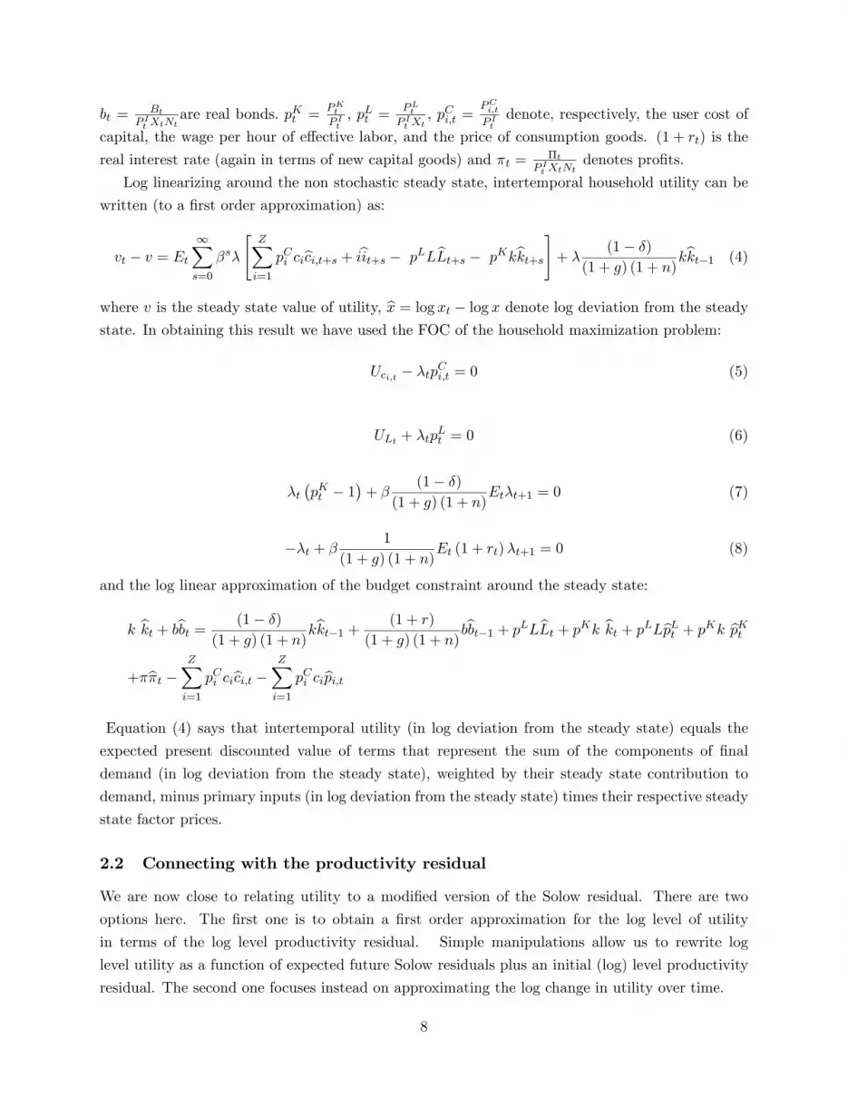
Log linearizing around the non stochastic steady state, intertemporal household utility can be
written (to a �rst order approximation) as:
vt � v = Et1Xs=0
�s�
"ZXi=1
pCi cibci;t+s + ibit+s � pLLbLt+s � pKkbkt+s#+ � (1� �)(1 + g) (1 + n)
kbkt�1 (4)
where v is the steady state value of utility, bx = log xt � log x denote log deviation from the steady
state. In obtaining this result we have used the FOC of the household maximization problem:
Uci;t � �tpCi;t = 0 (5)
ULt + �tpLt = 0 (6)
�t�pKt � 1
�+ �
(1� �)(1 + g) (1 + n)
Et�t+1 = 0 (7)
��t + �1
(1 + g) (1 + n)Et (1 + rt)�t+1 = 0 (8)
and the log linear approximation of the budget constraint around the steady state:
k bkt + bbbt = (1� �)(1 + g) (1 + n)
kbkt�1 + (1 + r)
(1 + g) (1 + n)bbbt�1 + pLLbLt + pKk bkt + pLLbpLt + pKk bpKt
+�b�t � ZXi=1
pCi cibci;t � ZXi=1
pCi cibpi;tEquation (4) says that intertemporal utility (in log deviation from the steady state) equals the
expected present discounted value of terms that represent the sum of the components of �nal
demand (in log deviation from the steady state), weighted by their steady state contribution to
demand, minus primary inputs (in log deviation from the steady state) times their respective steady
state factor prices.
2.2 Connecting with the productivity residual
We are now close to relating utility to a modi�ed version of the Solow residual. There are two
options here. The �rst one is to obtain a �rst order approximation for the log level of utility
in terms of the log level productivity residual. Simple manipulations allow us to rewrite log
level utility as a function of expected future Solow residuals plus an initial (log) level productivity
residual. The second one focuses instead on approximating the log change in utility over time.
8
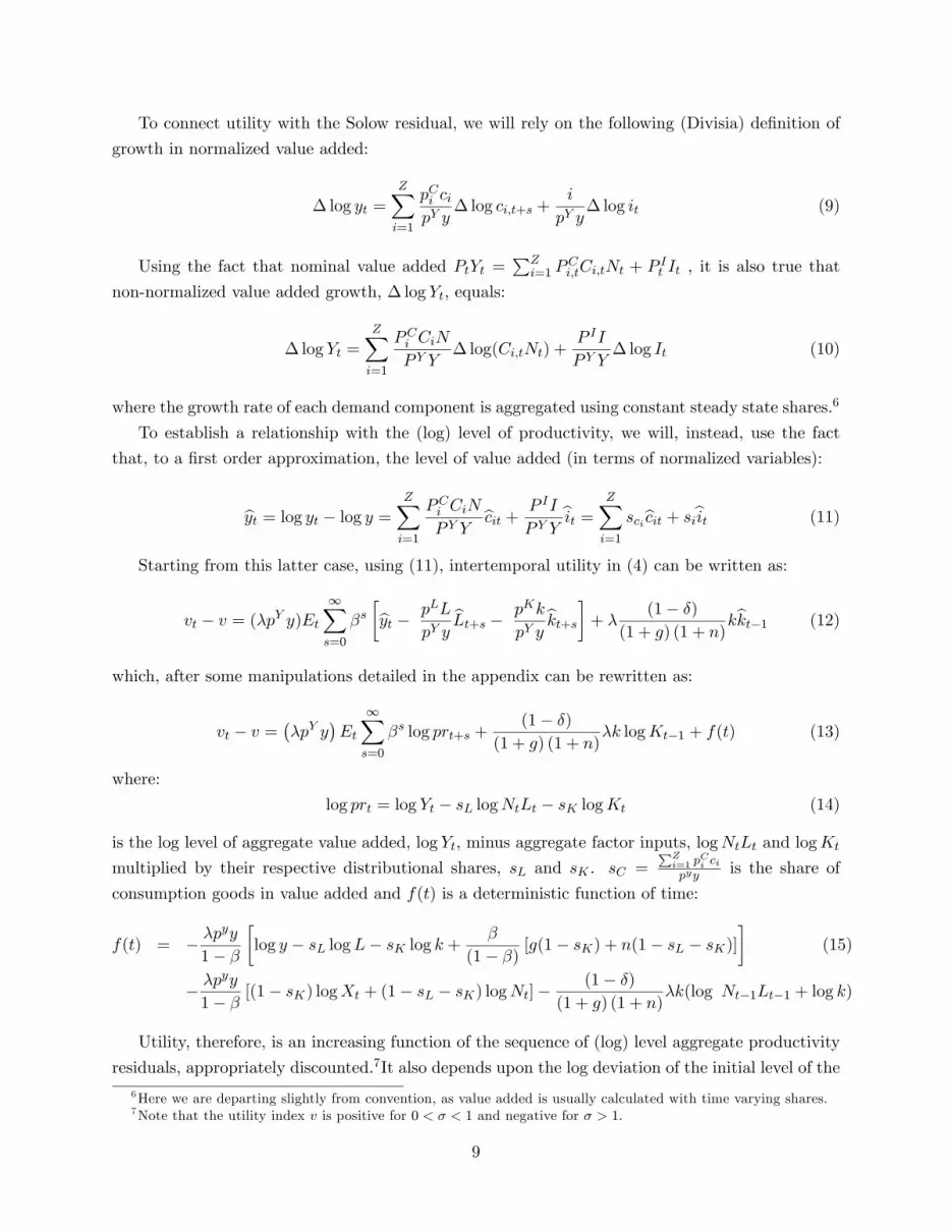
To connect utility with the Solow residual, we will rely on the following (Divisia) de�nition of
growth in normalized value added:
� log yt =
ZXi=1
pCi cipY y
� log ci;t+s +i
pY y� log it (9)
Using the fact that nominal value added PtYt =PZi=1 P
Ci;tCi;tNt + P
It It , it is also true that
non-normalized value added growth, � log Yt, equals:
� log Yt =
ZXi=1
PCi CiN
P Y Y� log(Ci;tNt) +
P II
P Y Y� log It (10)
where the growth rate of each demand component is aggregated using constant steady state shares.6
To establish a relationship with the (log) level of productivity, we will, instead, use the fact
that, to a �rst order approximation, the level of value added (in terms of normalized variables):
byt = log yt � log y = ZXi=1
PCi CiN
P Y Ybcit + P II
P Y Ybit = ZX
i=1
scibcit + sibit (11)
Starting from this latter case, using (11), intertemporal utility in (4) can be written as:
vt � v = (�pY y)Et1Xs=0
�s�byt � pLL
pY ybLt+s � pKk
pY ybkt+s�+ � (1� �)
(1 + g) (1 + n)kbkt�1 (12)
which, after some manipulations detailed in the appendix can be rewritten as:
vt � v =��pY y
�Et
1Xs=0
�s log prt+s +(1� �)
(1 + g) (1 + n)�k logKt�1 + f(t) (13)
where:
log prt = log Yt � sL logNtLt � sK logKt (14)
is the log level of aggregate value added, log Yt; minus aggregate factor inputs, logNtLt and logKtmultiplied by their respective distributional shares, sL and sK . sC =
PZi=1 p
Ci ci
pyy is the share of
consumption goods in value added and f(t) is a deterministic function of time:
f(t) = � �pyy
1� �
�log y � sL logL� sK log k +
�
(1� �) [g(1� sK) + n(1� sL � sK)]�
(15)
� �pyy
1� � [(1� sK) logXt + (1� sL � sK) logNt]�(1� �)
(1 + g) (1 + n)�k(log Nt�1Lt�1 + log k)
Utility, therefore, is an increasing function of the sequence of (log) level aggregate productivity
residuals, appropriately discounted.7It also depends upon the log deviation of the initial level of the6Here we are departing slightly from convention, as value added is usually calculated with time varying shares.7Note that the utility index v is positive for 0 < � < 1 and negative for � > 1:
9

capital stock, bkt�1; since for any sequence of productivity, welfare is higher if the consumer startswith an higher initial endowment of capital.
To establish the relationship with the Solow residual (a growth rate concept) there are two
options. One option is to use the fact that, for any variable x :
Etbxt+s = Et(log xt+s � log x) = Et sXi=1
(log xt+i � log xt+i�1) + log xt � log x
In the appendix we show that log level utility,(4), implies that per capita (log) intertemporal
utility can also be written as:
vt � v =�pY y
(1� �)Et1Xs=1
�s� log prt+s +�pY y
(1� �) log prt +(1� �)
(1 + g) (1 + n)�k logKt�1 + f(t) (16)
where � log prt denotes the "modi�ed" Solow productivity residual:
� log prt+s = � log Yt+s � sL� logNt+sLt+s � sK� log Kt+s (17)
We use the word "modi�ed," for two reasons. First, we do not assume that the distributional
shares of capital and labor add to one, as they would if there were zero economic pro�ts. Zero
pro�ts are guaranteed in the benchmark case with perfect competition and constant returns to scale,
but can also arise with imperfect competition and increasing returns to scale, as long as there is free
entry, as in the standard Chamberlinian model of imperfect competition. Second, the distributional
shares are calculated at their steady state values and, hence, are not time varying. Rotemberg and
Woodford (1991) argue that in a consistent �rst-order log-linearization of the production function
the shares of capital and labor should be taken to be constant, and Solow�s (1957) use of time-
varying shares amounts to keeping some second-order terms while ignoring others. Now log level
productivity has been written as a combination of expected future Solow residuals and one initial
productivity term in levels. Assume one is willing to make the assumption that an economy at time
t-1 was at the steady state, so that log yt�1� sL logLt�1� sK log kt�1 = log y� sL logL� sK log kIn this special case simple algebra shows that vt depends upon the expected present discounted
value of Solow residuals (from the present to in�nity).
vt � v =�pY y
(1� �)Et1Xs=0
�s� log prt+s + f0 (18)
where:
f0 =�pY y
(1� �)2 [g(1� sK) + n(1� sK � sL)] (19)
An alternative and more satisfactory way to illustrate the relationship between welfare and
the Solow residual (with no level term) is to return to (4) and take its di¤erence through time
10

(�vt = vt � vt�1): Using only the de�nition of value added in growth terms, equation (9), thegrowth rate of per capita utility can be written as follows:
�vt = �pyyEt
1Xs=0
�s� log prt+s + f1
+�pyy
1Xs=0
�s [Et log prt+s � Et�1 log prt+s]
+�pyy(1� �) k
(1 + g) (1 + n)
k
pyy� logKt�1 (20)
where Et� log prt+s represents the expected Solow residual while Et log prt+s �Et�1 log prt+s rep-resents the revision in expectations of the log level of the productivity residual, based on the new
information received between t-1 and t. In addition, � logKt�1 captures the change in the initial
endowment of capital. Finally, the constant f1 is:
f1 =�pY y
(1� �) [g(1� sK) + n(1� sK � sL)]�� (1� �) k(n+ g)(1 + g) (1 + n)
(21)
Note that the revision term in the second summation will reduce to a linear combination of
the innovations in the stochastic shocks a¤ecting the economy at time t. Moreover, if we assume
that the modi�ed Solow residual follows a simple stable �rst order autoregressive process, then the
current Solow residual, � log prt; is a su¢ cient statistic for all the terms in the �rst summation.
In this case, the growth in expected per capita utility is a linear function of today�s actual Solow
residual, of innovations at time t in the stochastic processes driving the economy and of the change
in initial endowment of capital.
2.3 Extensions
We now show that our method of using TFP to measure welfare can be extended to cover multiple
types of capital and labor, taxes, and government expenditure. The �rst extension modi�es our
baseline results in only a trivial way, but the others all require more substantial changes to the
formulas above. These results show that the basic idea of using TFP to measure welfare holds in
a variety of economic environments, but also demonstrate the advantage of deriving the welfare
measure from an explicit dynamic model of the household. The model shows exactly what mod-
i�cations to the basic framework are required in each case, and demonstrates that some of these
modi�cations are quantitatively signi�cant.
2.3.1 Multiple Types of Capital and Labor
The extension to the case of multiple types of labor and capital is immediate. For simplicity, we
could assume that each individual is endowed with the ability to provide di¤erent types of labor
11
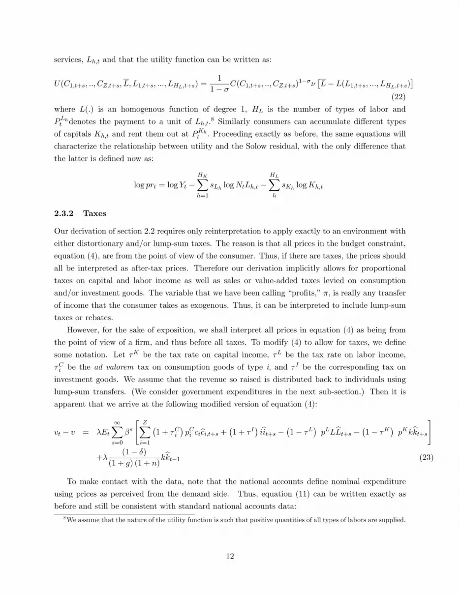
services, Lh;t and that the utility function can be written as:
U(C1;t+s; ::; CZ;t+s; L; L1;t+s; :::; LHL;t+s) =1
1� �C(C1;t+s; ::; CZ;t+s)1���
�L� L(L1;t+s; :::; LHL;t+s)
�(22)
where L(:) is an homogenous function of degree 1, HL is the number of types of labor and
PLht denotes the payment to a unit of Lh;t:8 Similarly consumers can accumulate di¤erent types
of capitals Kh;t and rent them out at PKht . Proceeding exactly as before, the same equations will
characterize the relationship between utility and the Solow residual, with the only di¤erence that
the latter is de�ned now as:
log prt = log Yt �HKXh=1
sLh logNtLh;t �HLXh
sKhlogKh;t
2.3.2 Taxes
Our derivation of section 2.2 requires only reinterpretation to apply exactly to an environment with
either distortionary and/or lump-sum taxes. The reason is that all prices in the budget constraint,
equation (4), are from the point of view of the consumer. Thus, if there are taxes, the prices should
all be interpreted as after-tax prices. Therefore our derivation implicitly allows for proportional
taxes on capital and labor income as well as sales or value-added taxes levied on consumption
and/or investment goods. The variable that we have been calling �pro�ts,��, is really any transfer
of income that the consumer takes as exogenous. Thus, it can be interpreted to include lump-sum
taxes or rebates.
However, for the sake of exposition, we shall interpret all prices in equation (4) as being from
the point of view of a �rm, and thus before all taxes. To modify (4) to allow for taxes, we de�ne
some notation. Let �K be the tax rate on capital income, �L be the tax rate on labor income,
�Ci be the ad valorem tax on consumption goods of type i, and � I be the corresponding tax on
investment goods. We assume that the revenue so raised is distributed back to individuals using
lump-sum transfers. (We consider government expenditures in the next sub-section.) Then it is
apparent that we arrive at the following modi�ed version of equation (4):
vt � v = �Et
1Xs=0
�s
"ZXi=1
�1 + �Ci
�pCi cibci;t+s + �1 + � I� ibit+s � �1� �L� pLLbLt+s � �1� �K� pKkbkt+s
#
+�(1� �)
(1 + g) (1 + n)kbkt�1 (23)
To make contact with the data, note that the national accounts de�ne nominal expenditure
using prices as perceived from the demand side. Thus, equation (11) can be written exactly as
before and still be consistent with standard national accounts data:8We assume that the nature of the utility function is such that positive quantities of all types of labors are supplied.
12

byt+s = ZXi=1
scibcit + sibit (24)
On the other hand, the national accounts de�ne factor prices as perceived by �rms, before
income taxes. Thus, the data-consistent de�nition of the welfare residual with taxes needs to be
based on a new de�nition of log prt. Rewrite equation (14) as:
log prt+s = log Yt+s ��1� �L
�pLLN
pY ylogNt+sLt+s �
�1� �K
�pKk
pY ylogKt+s (25)
= log Yt+s ��1� �L
�sL logNt+sLt+s �
�1� �K
�sK logKt+s
This new de�nition of log prt then needs to be applied to equations such as (12) and (13) in
section 2.2.
While it is easy to incorporate taxes into the analysis� as noted above, they are present im-
plicitly in the basic expressions derived in section 2.2� the quantitative impact of modeling taxes
explicitly can be large. Suppose that output is produced using an aggregate, constant-returns-to-
scale production function of capital, labor and technology, as in Solow�s classic (1957) paper. Then,
without distortionary taxes, only changes in technology change welfare.
Now suppose the average marginal tax rate on both capital and labor income is 30 percent, and
the share of consumption in output is 0.60. Suppose the government manages to raise aggregate
capital and labor inputs by 1 percent permanently without a change in technology (perhaps via
a small cut in tax rates). Then the �ow increase in utility is equivalent to an increase in steady-
state consumption of 0.5 percent. If the discount factor is 0.95 on an annual basis, the present
value of this policy change is equivalent to a one-year increase in consumption of 10 percent of the
steady-state level!
2.3.3 Government expenditure
With some minor modi�cation, our framework can be extended to allow for the provision of public
goods and services. We illustrate this under the assumption that government activity is �nanced
with lump-sum taxes. Using the results from the previous subsection, it is straightforward to extend
the argument to the case of distortionary taxes.
Assume that government spending takes the form of public consumption valued by consumers.
We rewrite the instantaneous utility function as
U(C1;t+s; ::; CZ;t+s; L; L1;t+s; :::; LHL;t+s) =1
1� �C(C1;t+s; ::; CZ;t+s;Gt+s)1���(L� Lt+s) (26)
whereG denotes per-capita public consumption, and we continue to assume that C(:) is homogenous
of degree one in its arguments. The relevant welfare residual in equation (4) now becomes:
13
vt�v = �Et1Xs=0
�s
"Uggbgt+s�
+
ZXi=1
pCi cibci;t+s + ibit+s � pLLbLt+s � pKkbkt+s#+� (1� �)(1 + g) (1 + n)
kbkt�1(27)
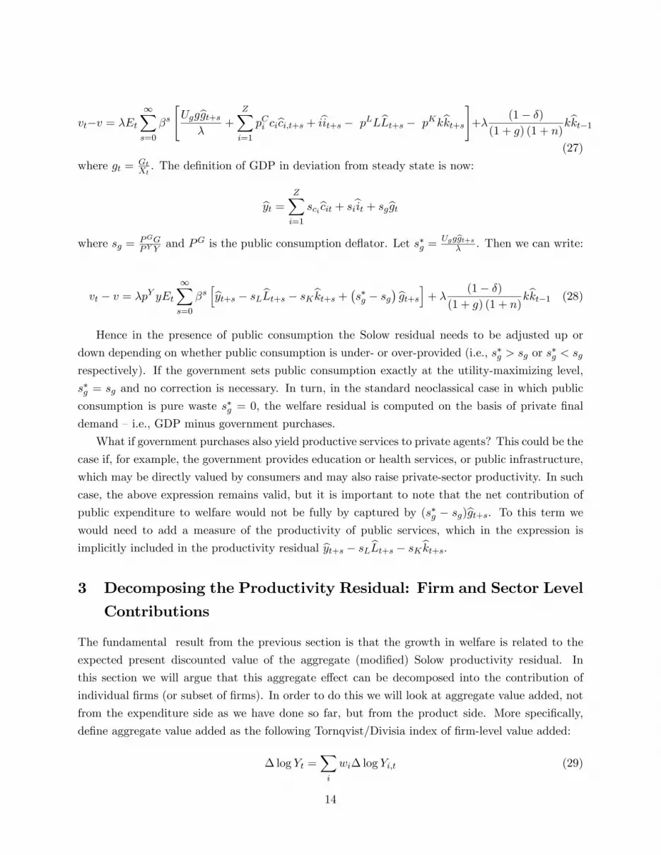
where gt = GtXt. The de�nition of GDP in deviation from steady state is now:
byt = ZXi=1
scibcit + sibit + sgbgtwhere sg = PGG
PY Yand PG is the public consumption de�ator. Let s�g =
Uggbgt+s� . Then we can write:
vt � v = �pY yEt1Xs=0
�shbyt+s � sLbLt+s � sKbkt+s + �s�g � sg� bgt+si+ � (1� �)
(1 + g) (1 + n)kbkt�1 (28)
Hence in the presence of public consumption the Solow residual needs to be adjusted up or
down depending on whether public consumption is under- or over-provided (i.e., s�g > sg or s�g < sg
respectively). If the government sets public consumption exactly at the utility-maximizing level,
s�g = sg and no correction is necessary. In turn, in the standard neoclassical case in which public
consumption is pure waste s�g = 0, the welfare residual is computed on the basis of private �nal
demand �i.e., GDP minus government purchases.
What if government purchases also yield productive services to private agents? This could be the
case if, for example, the government provides education or health services, or public infrastructure,
which may be directly valued by consumers and may also raise private-sector productivity. In such
case, the above expression remains valid, but it is important to note that the net contribution of
public expenditure to welfare would not be fully by captured by (s�g � sg)bgt+s. To this term we
would need to add a measure of the productivity of public services, which in the expression is
implicitly included in the productivity residual byt+s � sLbLt+s � sKbkt+s.3 Decomposing the Productivity Residual: Firm and Sector Level
Contributions
The fundamental result from the previous section is that the growth in welfare is related to the
expected present discounted value of the aggregate (modi�ed) Solow productivity residual. In
this section we will argue that this aggregate e¤ect can be decomposed into the contribution of
individual �rms (or subset of �rms). In order to do this we will look at aggregate value added, not
from the expenditure side as we have done so far, but from the product side. More speci�cally,
de�ne aggregate value added as the following Tornqvist/Divisia index of �rm-level value added:
� log Yt =Xi
wi� log Yi;t (29)
14

The corresponding index for producer prices is:
� logP Y t =Xi
wi� logPYi;t (30)
Moreover, one can easily show that the following is true as an approximation:
sK� logKt =Xi
wisK;i� logKi;t
and
sL� logNtLt =Xi
wisL;i� logNtLi;t
As a result the aggregate Solow residual can be written as the weighted sum (with value-added
weights) of the �rm-level Solow residuals. More speci�cally:
� log prt =Xi
wi� log prit
where � log prit is de�ned as:
� log prit = � log Yi;t � sK;i� logKi;t � sL;i� logNtLi;t (31)
We can use this result to examine the sectoral sources of productivity growth, which is the key
to welfare change, within a country. We can ask a variant of the same question for �rms, as we
explain in the results sub-section. Finally, we can compare cross-sectional summary statistics. For
example, we can ask whether small or large �rms contribute more to national welfare improvement.
4 Data and Measurement
Our main source of information is Amadeus, a comprehensive �rm-level pan-European database
developed by Bureau Van Dijk. For every �rm it provides data on the industry where it operates
(at the 4-digit NACE level), its location, the year of incorporation, the ownership structure and the
number of employees, in addition to the complete balance sheets and the pro�t and loss accounts.
The data set includes both publicly traded and non traded companies. We limit our analysis to a
subset of countries: Belgium, France, Great Britain, Italy, and Spain. We focus on manufactur-
ing companies with operating revenues greater than or equal to 2 million Euros and continuous
observations within the period of analysis. (We restrict ourselves to the balanced panel because
Amadeus does not supply census data; there is no way to distinguish between entry into the sample
and actual entry into the economy.)
We also use industry-level yearly data from the EU-KLEMS project, which provides output,
input and price data for industries at roughly the 2-digit level of aggregation across a large number
15
of countries up to 2005. These countries are mostly, but not exclusively, European; the project
also gives data for non-EU countries like Australia, Japan, Korea and the United States. The
EU-KLEMS data are extensively documented by O�Mahony and Timmer (2009).
In addition to the non-parametric welfare-relevant index numbers presented in the next section,
we will also estimate production functions using �rm level data, allowing the coe¢ cients to vary
across 2-digit industries for the period 1998-2005.9 Before 1998 the number of �rms in the survey
is signi�cantly smaller in most countries. Between 1998 and 2000 many �rms enter in the data
set. The coverage provided by the dataset varies across these countries. In 2005 the aggregated
sales of the �rms represented in Amadeus represent between 20 percent and 45 percent of the
manufacturing sector�s total production value, as documented in EU-KLEMS.
Our gross output proxy is (�rm level) revenues de�ated by the sectoral value added de�ator
obtained from the EU-KLEMS data set, at the 2 digit level. All de�ators used here will be at the 2
digit level and are obtained from EU-KLEMS. We are aware that using industry de�ators in place
of �rm-level prices can cause problems (Klette and Grilliches (1996)), but �rm-level price data for
output are not available in Amadeus. Our proxy for labor input is manpower costs de�ated by the
labor services de�ator. (For some countries, such as Italy, the number of employees �gure is not
reliable, since there is not a reporting requirement for the number of employees in the main section
of the balance sheet.) Capital is the historical value of tangible �xed assets divided by the price
index for investment. We have also experimented with the perpetual inventory method, obtaining
similar results. A measure for materials, intermediates and other services used in production
has been computed using the following formula: materials = Operating Revenues - (Operating
Pro�ts+Manpower costs+Depreciation). The �gure obtained in this way is then de�ated by the
materials and services de�ator. Given gross output and materials input, value added is constructed
as a Tornqvist/Divisia index.
5 Sources of Welfare Di¤erences
Welfare change depends on the expected present discounted value of expected TFP growth as
shown by equations (18) and (20). It is therefore important to investigate the time-series property
of TFP growth. We do so in Table 1, using annual data from EU-KLEMS up to 2005 for the entire
private economy for Belgium, France, Great Britain, Italy, and Spain. We use the measure of TFP
developed in EU-KLEMS, based on the assumption of zero pro�ts and time varying distributional
shares and present both country by country and pooled results. The persistence of TFP growth is
a key statistic, since it shows how the entire summation of expected productivity residuals changes
as a function of the new information about the TFP growth rate. For most countries the log level
of the TFP index is well described by an AR(1) stationary process around a country-speci�c linear
trend. Additional lags of log TFP are not signi�cant and the residual is white noise, as suggested
by the Lagrange Multiplier test for residual serial correlation. The only exception is Spain, where9The use of a �ner sectoral disaggregation is questionable if one wants to have enough �rms in each sector for
estimation purposes.
16
the coe¢ cient of log TFP (t-3) is signi�cantly di¤erent from zero at the 5% level and the LM test
rejects the hypothesis of no serial correlation (up to the third order). Thus, for most countries the
growth rate of TFP is well described by an ARMA(1,1) model. We henceforth focus on the current
TFP growth rate, since for most countries the data do not reject the proposition that the current
growth rate (or its innovation) gives all necessary information about the entire future path of TFP,
and hence welfare.
We �rst ask which sectors contributed the most to welfare change in these countries over the
period of our study through their contribution to aggregate TFP growth. The results are in Table 2.
We look at the contributions of �ve major industry groups: Manufacturing, Utilities, Construction,
Wholesale and Retail Trade and FIRE. For each country, we present in line 1 the mean of the
Tornqvist index of TFP growth for these industries, which represent the overwhelming majority
of private output. Interestingly, average TFP growth over this period is less than 1 percent per
annum, even for the leading economies, France and Britain. The sectoral decompositions are also
interesting. The next �ve lines give average sectoral TFP growth rates (not growth contributions,
which would multiply the growth rates by the respective sectoral weights, and give a mechanical
advantage to large sectors). Manufacturing makes a positive contribution for each country. The
contribution of FIRE (Finance, Insurance, Real Estate), on the other hand, is often negative,
especially in Britain, which has become a �nancial hub for the world.10 But the humble utility
sectors are the largest source of productivity growth on average (in every country other than Italy).
Alesina et al (2005) suggest an explanation for this pattern based on deregulation of the utilities
sectors in many European countries (with Italy a laggard in terms of the timing and pace of
deregulation).
In Table 3, we look at the contributions of di¤erent groups of �rms to welfare growth, now using
our �rm-level data from Amadeus for these countries. We now look at the average TFP growth
rates of small and large �rms, from 1998-2004. No very clear pattern emerges. Large �rms have
higher TFP growth rates in two countries (Belgium and Spain); small �rms have higher growth
rates in two others (Italy and Great Britain), and the contributions are basically identical in the
remaining country, France.
We can further decompose productivity di¤erences across countries by applying the following
decomposition, based on Griliches and Regev (1995). We wish to ask whether the di¤erence in the
productivity growth rate of any pair of countries is due to di¤erences in their sectoral compositions
or to di¤erences in the growth rates for each sector. Let i now index sectors (not �rms) and C be
one of the countries in our sample other than the UK.
10However, measures of both nominal and real �nancial sector output are often unreliable. See Wang, Basu andFernald (forthcoming) for a model-based method for constructing �nancial sector output. Basu, Inklaar and Wang(forthcoming) apply this theory to construct nominal bank output measures, and Inklaar and Wang (2007) providea theory-consistent measure of real bank output in the United States.
17
Xi
wCi � log prCit �
Xi
wUKi � log prUKit =Xi
(wCi + wUKi )
2(� log prCit �� log prUKit )
+Xi
(� log prCit +� log prUKit )
2(wCi � wUKi )
In Table 4, we examine the results of the Griliches-Regev (1995) decomposition, investigating
the sources of growth of each country�s TFP relative to that of Britain, which is the TFP growth
leader over our period. The �rst column describes the di¤erence in productivity change between
Great Britain and the other economies in our sample (and is of course negative in all cases). The
second column gives the amount of the di¤erence accounted for by cross country di¤erences in TFP
growth for each sector, while the third column gives the amount of the di¤erence due to di¤erences
in industrial structure (the share of each industry in the aggregate for that country). In most cases,
cross country di¤erences in the growth rate of the same sector account for the great majority of the
gap with the UK. The exception is France, which actually grows faster than Britain comparing the
same sector in the two countries, but loses nearly two-tenths of a percentage point of TFP growth
per year due to di¤erences in industrial structure.
In Table 5, we do an exercise designed to show whether the productivity patterns in each country
are related to cross-country di¤erences in the shape of the distribution of productivity growth rates
across �rms. This is an exercise in the spirit of Hsieh and Klenow (2009). However, Hsieh and
Klenow expended considerable e¤ort (and had to make a number of strong assumptions) in order
to isolate �rm-level technology within each country-sector. Our results show that if the object is
to investigate the reasons for di¤erences in welfare change across countries, it is not necessary (and
indeed not su¢ cient) to understand how technology di¤ers across �rms; we should concentrate on
di¤erences in the Solow residual instead. We do the following exercise. For our full sample of �rms
within each country, we calculate TFP, and then divide �rm-level TFP growth by TFP growth for
the aggregate of the �rms in that country. We then divide the range of productivity growth rates
into 10 bins, and ask what percentage of �rm value-added is produced by �rms in each standardized
productivity decile. (We experimented with dividing the range of growth rates more �nely, into
20 bins, with qualitatively similar results.) Finally, we ask how much faster or slower aggregate
TFP would have grown if the standardized distribution for the country had been replaced by the
standardized distribution for Great Britain.
The results are in Table 5. For ease of viewing the results, we also plot the distributions for
each country and the distribution for Britain in Figure 1. We �nd that replacing the distributions
in Belgium and Spain with the British distribution would actually have caused those two countries
to grow slightly more slowly. However, the same exercise for France and Italy shows that those
two countries would each have had half a percentage point higher TFP growth per year over the
full six years. This is a signi�cant di¤erence, especially for Italy where it approximately doubles
the annual TFP growth for our aggregate of �rms. Thus, there is some evidence that a portion of
18

the TFP growth di¤erences relative to Britain, which is the probably the least regulated and most
"US-like" of the countries in our sample, is driven by di¤erences in institutions that allow weak
�rms to linger or prevent strong �rms from expanding. The evidence is particularly strong in the
case of Italy, which has been a conspicuous laggard in its rate of productivity growth over the last
decade.
6 Decomposing the Productivity Residual:
The Role of Reallocation and Technology
The great bene�t of an index-number approach, such as the one we take in the previous section,
is that it provides interesting results without requiring formal econometrics. The cost is that
we cannot then identify the components of productivity growth, such as technical change or scale
economies. Having established that aggregate TFP is the natural measuring stick for aggregate
welfare, we now proceed to decompose aggregate TFP into components. We choose to work in
growth rates, since there are well-known di¢ culties in comparing TFP levels across industries
and countries. As we noted, while TFP growth is itself meaningful in welfare terms without any
additional assumptions, we need to make assumptions about �rm technology and behavior in order
to decompose it in a meaningful way. We use the decomposition of Basu and Fernald (2002), which
is derived by assuming that �rms minimize costs and are price-takers in factor markets, but may
have market power for the goods they sell and might produce with increasing returns to scale.
Some of the components in the decomposition we use can be clearly identi�ed as being due to
reallocation, since they depend on marginal products of identical inputs not being equalized across
�rms. Other components depend on aggregate distortions, such as the average degree of market
power and various tax rates.
6.1 Summary of the Basu and Fernald decomposition
Following Basu and Fernald (2002), in this paragraph we decompose changes in aggregate produc-
tivity into changes in aggregate technologies and changes in three non-technological components
re�ecting imperfections and frictions in output and factor markets. Suppose that each �rm i has
the following production function:
Qi = Fi(Ki; Li;Mi; T
Qi ) (32)
where Qi is the gross output, Ki; Li and Mi are inputs of capital, labor and materials, TQi is a
technology index and F i is an homogenous function. Assume that �rms are price takers in factor
markets but have market power in the output markets. Call PJi the price for factor J faced by
�rm i and �Qi the mark up that �rm i imposed over marginal costs. For any input J, let F iJ be the
marginal product. Firm i�s �rst order condition implies:
19

PiFiJ = �
Qi PJi (33)
Output growth, d logQi, can be written as:
d logQi = �Qi
hsQL;id logLi + s
QK;id logKi + s
QM;id logMi
i+F iTQTQi
F id log TQi = �
Qi d logX
Qi +
F iTQTQi
F id log TQi
where sQJ;i is the revenue share of input J out of gross output, d log TQi denotes technology growth
and d logXQi is revenue share weighted total input growth. Remember that our ultimate goal is
decomposing the aggregate Solow residual. In the national account identity in closed economy,
total expenditure equals the sum of �rms�value added. Consider the standard Divisia index of �rm
level value added:
d log Yi =d logQi � sQM;id logMi
1� sQM;i= d logQi �
sQM;i
1� sQM;i(d logMi � d logQi)
and de�ne the change in aggregate primary inputs, d logXi, as the share-weighted sum of the
growth rates of capital and labor:
d logXi =sQK;i
1� sQM;id logKi +
sQL;i
1� sQM;id logLi = sK;id logKi + sL;id logLi
After some algebra, taking into account that the �rms�value added productivity residual d log priequals d log Yi � d logXi, we obtain:
d log pri = (�i � 1)d logXi + (�i � 1)sQM;i
1� sQM;i(d logMi � d logQi) + d log Ti
where:
�i = �Qi
1�sQM;i
1��Qi sQM;i
d log Ti =F iTQ
TQiF i
d log TQi1��Qi s
QM;i
Let us move now to aggregate quantities. De�ne aggregate inputs as the simple sums of �rm-
level quantities: K =PIi=1Ki and L =
PIi=1 Li.
Now de�ne aggregate output growth as a Divisa index of �rm level value added:
d log Y =
IXi=1
wid log Yi
where wi is �rm i�s share of nominal value added: wi = P Yi Yi=PY Y and de�ne aggregate primary
input growth as:
20

d logX =sQK
1� sQMd logK +
sQL
1� sQMd logL = sKd logK + sLd logL
where sJ is the share of input J out of total value added. After some algebraic manipulation, d logX
can be written in terms of the weighted average of �rm level primary input growth: d logX =PIi=1wid logXi. Aggregate productivity growth, d log pr, is the di¤erence between aggregate output
growth d log Y and aggregate inputs growth d logX. Basu and Fernald shows that after some
manipulations, d log pr can be decomposed in the following way:11
d log pr = (�� 1)d logX + (�� 1)d logM=Q+R� +RM + d log T (34)
where:
� =PIi=1wi�i
d logM=Q =PIi=1wi
sQM;i
1�sQM;i
(d logMi � d logQi)
R� =PIi=1wi (�i � �) d logXi
RM =PIi=1wi (�i � �)
sQM;i
1�sQM;i
(d logMi � d logQi)
d log T =PIi=1wid log Ti
It is easy to provide an intuition for the welfare relevance of each term in which we have
decomposed aggregate productivity. The �rst term, (� � 1)d logX; is a direct consequence ofimperfect competition. Consumers would prefer to provide more labor and capital and consume
the extra goods produced, since their utility value exceeds the disutility of producing them. Hence
aggregate productivity and welfare increases with aggregate primary input growth, and this is true
even if �rms have the same markup. In this sense, (��1)d logX re�ects an aggregate distortion and
should not be counted as part of "reallocation," which we use as shorthand for allocative e¢ ciency.
The third term, R�; represents the increase in productivity and welfare coming from the fact
that primary inputs are directed towards �rms with higher-than-average markups, since higher
prices and markups express higher social valuation.
The terms (��1)d logM=Q and RM re�ect the fact that a markup greater than one reduces the
use of materials as well as primary inputs below the socially optimal level. This distortion is greater
the greater is the markup. Note that if materials had to be used in �xed proportion to output,
d logMi�d logQi would equal zero and so would both (�� 1)d logM=Q and RM . (In other words,the distortions regarding primary inputs would summarize fully the distortions in input use due to
markups that exceed one.) More speci�cally, (�� 1)d logM=Q re�ects the distortion generated byan average markup above unity and RM re�ects reallocation across �rms with di¤erent markups
(relative to �). Only the latter should be counted as part of reallocation. Finally the term d log T
11We are assuming here that the price paid by each �rm for capital and labor is the same. If it is allowed todi¤er, Basu and Fernald (2002) show that two additional terms should be added to the right hand side of (34):
RK � �PI
i=1 wisK;ihPKi�PKPKi
id logKi and RL � �
PIi=1 wisL;i
hPLi�PLPLi
id logLi. These input reallocation terms
represent gains from directing primary inputs towards �rms where they have higher social valuation.
21
represents the contribution to productivity and welfare of changes in aggregate technology.
The Basu and Fernald decomposition can be extended by disaggregating R� into a within sectors
and between sectors component. This is useful in assessing whether the gain from reallocation (if
any) occur because resources are reallocated across industries or within industries across �rms.
Basu and Fernald used industry level data in their empirical exercise so they could at best evaluate
the between component. (We say "at best" because if there are within-industry reallocation terms,
then Basu and Fernald�s estimation using industry-level data would not give a consistent estimate
of even the average industry markup, �. In general, one can estimate � correctly only by taking
the average of �rm-level markups, estimated using �rm-level data.) If one uses �rm-level data,
one can discuss the relative importance of the within and between components. RM can also be
decomposed into a within and between component, but there is a residual term.
Let P Y JY J =Pi�J P
Yi Y
Ji be the total value added produced in industry J , w
J = P Y JY J=P Y Y
the share of industry J out of aggregate output and wJi = P Yi YJi =P
Y JY J the share of value
added of �rm i in industry J . Denote with Qi a �rm gross output and with PQi its price. Then
wQJi = PQi QJi =P
QJQJ , where PQJQJ =Pi�J P
Qii Q
J ; represents the �rm share of industry gross
output. Finally, the primary inputs growth in industry J is d logXJ = sJKd logKJ + sJLd logL
J ,
where sJK =Pi�J PK;iKi
PY JY Jand sJL =
Pi�J PL;iLiPY JY J
. De�ne RJ� and RJ�as the industry equivalent of the
reallocation terms R� and RM when aggregating over industry J rather than the entire economy, i.e.
RJ� =Pi�J w
Ji
��i � �J
�d logXi and RJM =
Pi�J w
Ji
��i � �J
� sQM;i
1�sQM;i
(d logMi � d logQi), where
�J =Pi�J w
Ji �i. We can decompose the reallocation term for primary inputs, R�; into a within
and a between component (denoted by superscripts W and B, respectively) as follows:
R� = RW� +RB�
where RW� =PKJ=1w
JRJ� and RB� =
PKJ=1w
J��J � �
�d logXJ :Note that the between component
can be calculated on the basis of industry data only.
The decomposition for the reallocation term for materials, RM , is instead:
RM = RWM +RBM +Rw�wQ
whereRWM =PKJ=1w
JRJM ; RBM =
PKJ=1w
J��J � �
�(d logQJ�d log Y J) andRw�wQ =
PKJ=1w
J��J � �
�( wJi � w
QJi )d logQi: In the between component, d log Y J =
Pi�J w
Ji d log Yi is the Divisia index
of industry value added,. d logQJ =Pi�J w
QJi d logQi is the Divisia index of gross output (using
wQJi as weights). The residual term, Rw�wQ , re�ects the di¤erence between value added weights
and gross output weights in aggregating �rm level gross output within an industry.
7 Econometric Framework
The modi�ed Solow productivity residual can be essentially calculated from the data and requires
no estimation if the distributional shares are observable (or if we observe the labor share and
22

assume approximately zero pro�ts). However, in order to break down the productivity residual
into components that re�ect aggregate distortions, reallocation and technology growth we must
obtain estimates of the markups and of technology growth. We will do that by assuming that the
(gross) production function in sector j is Cobb Douglas:
logQit = "jL logLit + "
jK logKit + "
jM logMit + �jt + �i + !it (35)
where i denotes �rms (i = 1; ::; Ij), t time (t = 1; ::; Tj), and small case variables logs. �jt is an
industry speci�c common component of productivity, �i a time invariant �rm level component and
!it an idiosyncratic component. In our application using the Amadeus data set, Tj is small and Njlarge.
We will experiment with di¤erent estimation methods: OLS, LSDV, Olley and Pakes, Di¤erence
and System GMM (assuming that !it is either serially uncorrelated, or that it follows an AR(1)
process). The advantages and disadvantages of each choice are well known, although there is no
agreement on which estimator one should ultimately choose. One fundamental estimation problem
is the endogeneity of the input variables, which are likely to be correlated both with �i and !it.
Correlation with !it may re�ect both simultaneity of input choices or measurement errors. Given
the shortness of the panel, elimination of �i through a within transformation is not the appropriate
strategy. Di¤erencing of (35) and application of the di¤erence GMM estimator (Arellano and Bond
(1991)) is a possibility, but appropriately lagged values of the regressors may be poor instruments if
inputs are very persistent. Application of the GMM System estimator (Blundell and Bond (1998)
and Blundell and Bond ( 2000) is probably a better option. An alternative approach is the one
proposed by Olley and Pakes (1996). This estimator addresses the simultaneity (and selection)
problem by using �rm investment as a proxy for unobserved productivity and requires the presence
of only one unobserved state variable at the �rm level and monotonicity of the investment function.
We are not interested to take a stand in this paper on which one is the preferable estimation
strategy. Fortunately for us, the results of the decomposition are insensitive to the choice of a
particular estimator.
Having obtained estimates of the output elasticity for each factor we will recover the �rm speci�c
markup from the �rst order conditions for materials, equation (33). In the Cobb Douglas case, this
can be expressed as:
b�Qi = b"jMsQM;i
(36)
where sQM;i is the time average of the �rm speci�c revenue share of materials for �rm i: A hat
denotes estimated values. We have chosen to focus on the FOC for materials because they are
likely to be the most a �exible input. Whereas the labor share, sQL;i; can be easily recovered from
the data, the same is not true for the capital share, sQK;i, unless one is willing to make assumptions
about the user cost of capital, which is problematic in the presence of �rm heterogeneity in the cost
of �nance. We have recovered the capital share from estimates of the markup described above and
23

of the elasticity of output with respect to capital, using:
sQK;i =b"jKb�Qi (37)
Alternatively we have obtained sQK;i from:
ski = 1� sQL;i � sQM;i �
�iYi= 1� sQL;i � s
QM;i � (1�
b�jb�Qi ) (38)
where b�j = b"jK +b"jL +b"jM is the degree of returns to scale in sector j. The result are robust to this
choice.
8 Results
We will discuss now the empirical results obtained when the production function is estimated on
the �rm level data contained in Amadeus for Belgium, France, Great Britain, Italy, Spain over the
period 1998-2005. To avoid overburdening the reader, we report results for selected estimators
(OLS, System GMM, and Olley and Pakes) for only one of our countries, Belgium.
The estimation results for the elasticity of output with respect to each factor, for constant
returns to scale and for average markups are reported in the tables 6, 7, and 9: Estimates are pretty
standard and vary somewhat across estimators. Recall that materials include services together with
materials and intermediates. The degree of returns to scale is very close to one in most sectors
using OLS and System GMM, while it is slightly smaller, but still close to one, with the Olley and
Pakes estimator. The estimate of "jK is greater for the OLS estimator and the smallest for the Olley
and Pakes estimator. For �ve sectors it is negative using the GMM System estimator with serially
uncorrelated errors, although not signi�cantly so. The test of overidentifying restrictions and the
test of second order serial correlation for the GMM System do not suggest major misspeci�cation
issues for most sectors, which leads us to focus on this version of the GMM estimator, instead of the
one allowing for an AR(1) error component in the level equation. The average estimated markup,
obtained using (36), exceeds one in all sectors, whatever the estimator used. Moreover it is strictly
greater than one for 64% of �rms, using OLS, 70% using System GMM, and 63% using Olley and
Pakes.
We �nd markup estimates that are quite reasonable compared to existing estimates in the micro-
econometric literature 12, albeit somewhat high relative to the macro literature. The numerical
estimates in Tables 6 through 9, usually in the range of 1.10 to 1.25, seem quite small, but one
needs to remember that these are markups on gross output. Converting to markups on value
added using a representative materials share of 0.7, the markups are in the range of 1.43 to 3.
Similarly, the implied pro�t rates are a bit on the high side. Using equation 38, the pro�t rate can
12For example, Dobbelaure and Mairesse (2008) �nd very similar markups using panel data for French �rms.
24

be calculated as (1� b�jb�Qi ). Taking constant returns as our modal estimate, the markup range justdiscussed corresponds to pro�t rates in the range of 9 to 20 percent, expressed as a percentage of
gross output.
Our estimates of the markup and thus of the pro�t rate are probably upper bounds. We do not
control for variations in �rm-level input utilization (changes in the number of shifts or variations in
labor e¤ort), except through our use of time �xed e¤ects. Thus, we remove variations in utilization
due to common industry e¤ects but not due to �rm-speci�c demand variation over time. Basu
(1996) suggests that variable utilization is likely to bias upward the output elasticity of materials
in particular, which is the parameter that has the largest impact on our estimates of markups and
pro�t rates. Unfortunately, we do not have the �rm-level data on hours worked per employee that
would be necessary to implement the utilization control derived from the optimizing model of Basu,
Fernald and Kimball (2006). Thus, our estimates of the average distortions coming from markup
pricing, as summarized by the �rst two terms in equation (34) are likely to be on the high side.
But the fact that our estimated average markups are large does not create any particular bias in
our estimates of the reallocation terms, which are our particular focus, since the reallocation terms
involving markups depend on the gaps between �rm-level and average markups.
In light of this discussion, it is interesting to look at the estimates of the various reallocation
terms for our sample of six countries, which are presented in Tables 10 and 11. In Table 10 we
report for each country in our sample, average productivity growth, d log pr, the sum of aggregate
distortions, (��1)d logX+(��1)d logM=Q, the sum of the reallocation terms for primary factorsand materials, R� + RM , and technology growth, d log T . The last column reports as residual the
di¤erence between productivity, on the one hand, and the sum of aggregate distortions, of the
reallocation terms, and of technological progress, on the other, i.e. the di¤erence between the left
hand side and the right hand side of (34). This equation may not hold as an equality for three
reasons: �rst we do not observe the true value of the markup, but only its estimated value; (ii)
whereas the labor share is observed in the data, calculations of the capital share depends upon a
zero pro�t assumptions or an estimate of the markup and of the degree of returns to scale; (iii) as
Basu and Fernald (2002) show, if the price paid for capital and labor di¤ers across �rms, additional
terms involving the di¤erence of factor prices for each �rm from the average, multiplied by each
factor growth rate will appear on the right hand side of (34).13
First of all, we see from Table 10 robust average annual productivity growth for all countries in
our sample of large �rms. The case of Italy is particularly striking, since our sample of �rms has
an average productivity growth rate, d log pr, of 2.8 percent, while the EU-KLEMS database shows
that for all of Italian manufacturing average TFP declined at a rate of 1.2 percent per year over
our sample period. Second, we see that technical change was also positive for all countries, and
13See footnote 11. Petrin, Reiter and White (2009) argue that changes in �xed costs create yet another gapbetween the two sides of equation (34). However, changes in �xed costs are equivalent to an additive technologyshock, and to a �rst-order approximation both additive and multiplicative technology shocks are already incorporatedinto the estimate of dlogT . Thus, changes in �xed costs are not an additional gap between productivity growth andtechnological change.
25

over 1 percent per year in all countries except Spain, where it averaged 0.5 percent. The strongest
rates of technical change, in excess of 4 percent per year, were registered in France, which is usually
found to be a high-productivity country in most cross-country studies, and in the United Kingdom,
which had 2.2 percent average TFP growth in manufacturing over this time period.
Before discussing the results on reallocation, note that the residual is sizeable and we decide to
allocate it to the aggregate distortion, reallocation, and technology growth component in proportion
to their relative size. In Table 11 we report the proportion of aggregate productivity accounted
for by each component, after this adjustment. The results suggest, �rst, that in most countries
most of productivity growth is accounted by technology growth. More speci�cally, technological
progress accounts for the totality of productivity growth in Great Britain and in France, for a
large fraction in Italy (.66%) and for a sizeable, but smaller fraction in Belgium and Spain (43%
and 21% respectively). Second, aggregate distortions are quite important in Spain Belgium, and
Italy, where they account for 85%, 55%, and 33% of productivity growth respectively. They are,
instead rather small in Great Britain and in France. The reallocation terms for primary factors or
materials accounts for a small proportion of productivity growth in all countries.14 It follows that,
unless one is willing to treat the entire residual as part of reallocation term, factor reallocation
does not appear to be an important component of productivity growth.15 Here the nature of the
sample may work against �nding strong results, since most of the �rms are quite large in all the
years they are observed. Reallocation e¤ects are most clearly apparent when �rms that are small
initially grow to a large size due to their superior productivity. There are probably fewer such
�rms in our sample than in the population, thus reducing the quantitative impact of reallocation.
Petrin, White and Reiter (2009) come to the di¤erent conclusion that reallocation represents a large
fraction of productivity growth, using manufacturing plant level data for the US. They calculate
their reallocation term as the di¤erence between a Divisia index of �rm level productivity growth
and a Divisia index of technology growth. Thus, they include aggregate distortions as part of
reallocation, which should not be the case if one wants to estimate and index of allocative e¢ ciency
strictly de�ned. We also �nd that aggregate distortions can be substantial for some countries.16
Finally, although reallocation of factors towards uses where they have a higher social valuation
has not been a large part of the improvement in productivity and welfare for the sample period
we have analyzed, does not mean that a benevolent central planner could not achieve large welfare
improvement from factor reallocation. This distinction between the historical decomposition we
have presented and what could be potentially obtained should be kept in mind when drawing
inferences from these results.14Because the reallocation term is so small, not much is learned from presenting its the decomposition in a within
and between component.15 If we treat the residual as re�ecting the di¤erence in primary factor prices faced by �rms and treat it entirely as
part of the reallocation term, as in Basu and Fernald (2002), reallocation would account for approximately a third ofproductivity growth in Great Britain.16Petrin, White and Reiter (2009) implement the decomposition proposed by Petrin and Levinsohn (2008) which
is a variant of the Basu and Fernald (2002) decomposition.
26

9 Conclusions
We show that the present value of aggregate TFP growth, for a given initial endowment of capital,
is a complete welfare measure for a representative consumer, up to a �rst-order approximation. This
result rigorously justi�es TFP, rather than technical change or labor productivity, as the central
statistic of interest in any exploration of productivity, at all levels of aggregation. Importantly,
the result holds even when TFP is not a correct measure of technical change, for example due
to increasing returns, externalities, or imperfect competition. It also suggests that productivity
decompositions should be oriented towards showing how particular features or frictions in an econ-
omy either promote or hinder aggregate TFP growth, which is the key to economic welfare. Our
theoretical results point to a key role for the persistence of aggregate TFP growth, since welfare
change is related to the entire expected time path of productivity growth in addition to the current
growth rate. Finally, our derivation shows that in order to create a proper welfare measure, TFP
has to be calculated using prices faced by households rather than prices facing �rms. In modern,
developed economies with high rates of income and indirect taxation, the gap between household
and �rm TFP can be considerable.
We use these central results to show that one can explore the sources of welfare change using
both non-parametric index numbers and formal econometrics. The non-parametric approach has
the great advantage of simplicity, and avoids the need to address issues of econometric identi�cation.
Many interesting cross-country comparisons can be performed using the index-number approach,
including calculating summary statistics of allocative e¢ ciency for each country based on �rm-
level data. However, if one wants to ask how much of aggregate TFP growth is due to technical
change, as opposed to scale economies or allocative ine¢ ciency, one does need to make additional
assumptions and estimate production functions at the �rm level. We show how one can decompose
aggregate TFP growth in such a manner using �rm-level data.
The results suggest that in the majority of OECD countries we have analyzed (Belgium, France,
Great Britain, Italy, and Spain) most of productivity growth in manufacturing is accounted for by
technology growth. This is particularly true for Great Britain and France. Moreover, aggregate
distortions are quite important in many countries, such as Spain, Belgium, and Italy. Finally, the
reallocation terms for primary factors or materials account for a small proportion of productivity
growth in all countries over the period 1995-2005. We will explore in future research whether this
result extends to other countries or time periods, or to other data sets less biased towards larger
�rms.
27

References
[1] Abel, A.B., 2003. The E¤ects of a Baby Boom on Stock Prices and Capital Accumulation in
the Presence of Social Security. Econometrica 71(2), 551-578
[2] Alesina, A., Ardagna, S., Nicoletti, Schiantarelli, F., 2005. Regulation and investment. Journal
of European Economic Association 3(4), 1-35
[3] Arellano, M., Bond, S., 1991. Some tests of speci�cation for panel data: Monte Carlo evidence
and an application to employment equations. Review of Economic Studies 14, 328-352
[4] Baker, D., Rosnick, D., 2007. "Usable productivity" growth in the US: an international com-
parison, 1980-2005. International Productivity Monitor
[5] Blundell, R., Bond, S., 1998. Initial conditions and moment restrictions in dynamic panel
models. Journal of Econometrics 87, 115-143
[6] Blundell, R., Bond, S., 2000. GMM estimation with persistent panel data: an applications to
production functions. Econometric Review 87, 115-143
[7] Basu, S., Fernald, J.G., 2002. Aggregate productivity and aggregate technology. European
Economic Review 46, 963-991
[8] Basu, S., Fernald J., Kimball M., 2006. Are Technology Improvements Contractionary?. Amer-
ican Economic Review 96 (5), 1418-1448
[9] Basu, S., Fernald, J.G., Shapiro, M.D., 2003. Productivity Growth in the 1990s: Technology,
Utilization, or Adjustment? NBER Working Paper 8359
[10] Basu, S., Inklaar, R., Wang C.J, forthcoming. The Value of Risk: Measuring the Service
Output of U.S. Commercial Banks. Economic Inquiry.
[11] Dobbelaere S., Mairesse J., 2008. Panel data estimates of the production function and product
and labor market imperfections. NBER Working Paper 13975
[12] Domar, E.D., 1961. On the measurement of technical change. Economic Journal 71, 710-729
[13] Grilliches, Z., Regev, H., 1995. Productivity and �rm turnover in Israeli industry. Journal of
Econometrics 65, 175-203
[14] Hellerstein, J.K., Neumark, D., 2008. Workplace Segregation in the United States: Race,
Ethnicity, and Skill. The Review of Economics and Statistics 90(3), 459-477
[15] Hsieh, C.T., Klenow, P.J., 2007. "Misallocation and Manufacturing TFP in China and India,"
NBER Working Papers 13290
28

[16] Hulten, C.R, 1978. Growth accounting with intermediate inputs, The Review of Economic
Studies 45, 511-518
[17] Inklaar, R., Wang, J.C., 2007. Not Your Grandfather�s Bank Any More? Consistent Mea-
surement of Non-Traditional Bank Output. mimeo, University of Groningen and Federal Re-
serve Bank of Boston
[18] King, R.G., Plosser, C.I., Rebelo, S.T., 1988. Production, growth and business cycles. Journal
of Monetary Economics 21, 195-232
[19] Klette, T.J., Griliches, Z., 1996. The Inconsistency of Common Scale Estimators When Output
Prices Are Unobserved and Endogenous. Journal of Applied Econometrics 11(4), 343-61
[20] Nordhaus, W., Tobin, J., 1972. Is growth obsolete? NBER General Series 96
[21] O�Mahony, M., Timmer, M.P., 2009. Output, Input and productivity measures at the industry
level: the EU KLEMS database. Economic Journal 119, pp.F374-F403
[22] Olley, S., Pakes, A., 1996, The dynamics of productivity in the telecommunications equipment
industry. Econometrica 64, 1263-1297
[23] Petrin, A., Levinsohn, J., 2009. Measuring Aggregate Productivity Growth Using Plant-Level
Data. Unpublished.
[24] Petrin, A., White, K., Reiter, J.P., 2009. The impact of plant-level resource reallocations and
technical progress on U.S. macroeconomic growth. Unpublished.
[25] Wang, C.J., Basu, S., Fernald, J.G., forthcoming In W. Erwin Diewert, John Greenlees and
Charles Hulten, eds., Price Index Concepts and Measurement
[26] Weitzman, M., 1976. On the welfare signi�cance of national product in a dynamic economy.
Quarterly Journal of Economics 90, 156-162.
[27] Weitzman, M., 2003. Income capital and the maximum principle. Harvard University Press,
Cambridge.
29

A Appendix A: Derivations
A.1 Making the problem stationary
The representative household maximizes intertemporal utility:
Vt =1Xs=0
1
(1 + �)sNt+sH
U(C1;t+s; ::; CZ;t+s;L� Lt+s) (A.1)
where Ci;t+s is the capita consumption of good i at time t+s, Lt+s are hours of work per capita, L
is the time endowment, and Nt+s population. H is the number of households, assumed to be �xed
and normalized to one from now on. Consider the laws of motion for Nt and for Xt, where the
latter denotes Harrod neutral technological progress (so that total labor input in e¢ ciency units is
(NtXtLt):
Nt = N0(1 + n)t (A.2)
Xt = X0(1 + g)t (A.3)
and normalize H = 1.
We can rewrite the utility function as:
Vt = Nt
1Xs=0
(1 + n)s
(1 + �)sU(C1;t+s; ::; CZ;t+s;L� Lt+s) (A.4)
For a well de�ned state in which hours of work are constant we assume that the utility function
has the King Plosser and Rebelo form(1988):
U(C1;t+s; ::; CZ;t+s;L� Ls) =1
1� �C(C1;t+s; ::; CZ;t+s)1���(L� Lt+s)
We assume that C() is homogenous of degree 1. De�ne ci;t+s =Ci;t+sXt+s
. We can rewrite the utility
function in the following form:
U(C1;t+s; ::; CZ;t+s;L� Lt+s) =1
1� �Xt+sC(c1;t+s; ::; cZ;t+s)1���(L� Lt+s)
or
U(C1;t+s; ::; CZ;t+s;L� Ls) = (1 + g)s(1��)X(1��)t
1
1� �C(c1;t+s; ::; cZ;t+s)1���(L� Lt+s)
Inserting this into Vt, we get:
Vt = NtX(1��)t
1Xs=0
�sU(c1;t+s; ::; cZ;t+s;L� Lt+s) (A.5)
30

where: � = (1+n)(1+g)1��
(1+�) .
A.2 Budget constraint
Start from the usual budget constraint:
P It Kt +Bt = (1� �)P It Kt�1 + (1 + it)Bt�1 + PLt LtNt + PKt Kt +�t �ZXi=1
PCi;tCi;tNt (A.6)
Divide both sides by P It XtNt to get:
KtXtNt
+Bt
P It XtNt= (1� �) Kt�1
Xt�1Nt�1
Xt�1Nt�1XtNt
+ (1 + it)Bt�1
P It�1Xt�1Nt�1
P It�1P It
Xt�1Nt�1XtNt
+PLtP It
LtNtXtNt
+PKtP It
KtXtNt
+�t
P It XtNt�
ZXi=1
PCi;t
P It
Ci;tNtXtNt
De�ne: kt = KtXtNt
, bt = BtP It XtNt
, pKt =PKtP It, pLt =
PLtP It Xt
, pCi;t =PCi;tP It; (1 + rt) =
(1+it)(1+�t)
, �t = �tP It XtNt
.
The budget constraint can be rewritten as:
kt + bt =(1� �)
(1 + g) (1 + n)kt�1 +
(1 + rt)
(1 + g) (1 + n)bt�1 + p
Lt Lt + p
Kt kt + �t �
ZXi=1
pCi;tci;t (A.7)
A.3 Optimality conditions
The representative household maximizes normalized intertemporal utility, vt = Vt
NtX(1��)t
, subject
to the budget constraint. The Lagrangean for this problem is:
Lt = Et1Xs=0
�sfU(c1;t+s; ::; cZ;t+s;L� Lt+s)
+�t (�kt � bt +(1� �)
(1 + g) (1 + n)kt�1 +
(1 + rt)
(1 + g) (1 + n)bt�1 + p
Lt Lt + p
Kt kt + �t �
ZXi=1
pCi;tci;t)g
The FOCs are:
Uci;t � �tpCi;t = 0 (A.8)
ULt + �tpLt = 0 (A.9)
31

�t�pKt � 1
�+ �
(1� �)(1 + g) (1 + n)
Et�t+1 = 0 (A.10)
��t + �t1
(1 + g) (1 + n)Et (1 + rt)�t+1 = 0 (A.11)
A.3.1 Approximation around SS
De�ne with bx = log xt � log x the log deviation from the steady state of a variable (x is the steady
state value of xt). Loglinearizing the problem around the steady state:
Lt � L = Et[
1Xs=0
�s(
ZXi=1
Ucicibci;t+s + ULtLbLi;t+s+�pLLbLi;t+s � � ZX
i=1
pCi cibci;t+s + �(pK � 1)kbkt+s � �bbbt+s)+
1Xs=0
�s+1��
(1� �)(1 + g) (1 + n)
kbkt+s + � (1 + r)
(1 + g) (1 + n)bbbt+s�
1Xs=0
�s
��1 + (1� �)
(1 + g) (1 + n)
�(k + b) + pLL+ pKk + � �
ZXi=1
pCi ci
!b�t+s+
1Xs=0
�s�
pLLbpLt+s + pKk bpKt+s � ZX
i:0
pCi;tcibpi;t+s + �b�t+s + rb
(1 + g) (1 + n)brt+s!]
+�(1� �)
(1 + g) (1 + n)kbkt�1 + � (1 + r)
(1 + g) (1 + n)bbbt�1
At an optimum, Lt�L = vt� v and the �rst four lines equal zero (using the optimality conditionsevaluated at the steady state):
vt � v = Et
1Xs=0
�s�
pLLbpLt+s + pKk bpKt+s � ZX
i:0
pCi;tcibpi;t+s + �b�t+s + rb
(1 + g) (1 + n)brt+s!
+�(1� �)
(1 + g) (1 + n)kbkt�1 + � (1 + r)
(1 + g) (1 + n)bbbt�1 (A.12)
Now log linearize the budget constraint:
k bkt + bbbt � (1� �)(1 + g) (1 + n)
kbkt�1 � (1 + r)
(1 + g) (1 + n)bbbt�1 � pLLbLt � pKk bkt � pLLbpLt � pKk bpKt
��b�t � rb
(1 + g) (1 + n)brt+s + ZX
i=1
pCi cibci;t + ZXi=1
pCi cibpi;t = 032

Using this result and the fact that bt = 0 in equilibrium, and hence bbt = 0 in (A.12), we obtain:
vt = v + Et
1Xs=0
�s�
"ZXi=1
pCi cibci;t+s + kbkt+s � (1� �)(1 + g) (1 + n)
kbkt+s�1 � pLLbLt+s � pKk bkt+s#
+�(1� �)
(1 + g) (1 + n)kbkt�1 (A.13)
Notice that the law of motion of capital: Kt = (1 � �)Kt�1 + It, can be rewritten as: KtXtNt
=
(1� �) Kt�1Xt�1Nt�1
Xt�1Nt�1XtNt
+ ItXtNt
which after some algebra becomes:
kt =(1� �)
(1 + g) (1 + n)kt�1 + it
Di¤erentiating it around the steady state, we get:
kbkt = (1� �)(1 + g) (1 + n)
kbkt�1 + ibitInserting this equation into equation A.13 we get:
vt = v + Et
1Xs=0
�s�
"ZXi=1
pCi cibci;t+s + ibit+s � pLL bLt+s � pKk bkt+s#
+�(1� �)
(1 + g) (1 + n)kbkt�1 (A.14)
A.4 Connecting the level of productivity to the level of welfare
De�ne value added (for normalized variables in deviation from steady state) as:
byt = log yt � log y = ZXi=1
PCi CiN
P Y Ybcit + P II
P Y Ybit = ZX
i=1
scibcit + sibit (A.15)
Inserting this equation into (A.14), we get:
vt = v + Et
1Xs=0
�s�pY yhbyt � sL bLt+s � sK bkt+si+ � (1� �)
(1 + g) (1 + n)kbkt�1 (A.16)
Using the de�nition of the normalized variable, this can be rewritten as:
vt = v +��pY y
�Et
1Xs=0
�s�(log
Yt+sNt+sXt+s
� log y)� sL(logLt+s � logL)� sK(logKt+s
Nt+sXt+s� log k)
�+�
(1� �)(1 + g) (1 + n)
k(logKt�1
Nt�1Xt�1� log k) (A.17)
33

or:
vt = v+��pY y
�Et
1Xs=0
�s [log Yt+s � sL log Nt+sLt+s � sK logKt+s]+(1� �)
(1 + g) (1 + n)�k logKt�1+f(t)
(A.18)
where:
f(t) = � �pyy
1� �
�log y � sL logL� sK log k +
�
(1� �) [g(1� sK) + n(1� sL � sK)]�
� �pyy
1� � [(1� sK) logXt + (1� sL � sK) logNt]�(1� �)
(1 + g) (1 + n)�k(log Nt�1Lt�1 + log k)
De�ne aggregate productivity (in log levels) as: log prt = log Yt � sL logNtLt � sK logKt. No-tice that we are de�ning productivity with constant shares (which is appropriate for a �rst order
approximation). Using this de�nition, the equation above can be rewritten as:
vt � v =��pY y
�Et
1Xs=0
�s log prt+s +(1� �)
(1 + g) (1 + n)�k logKt�1 + f(t) (A.19)
A.5 Connecting the aggregate Solow residual with the level of welfare
Now de�ne: �t+s =PZi:0 p
Ci ci log ci;t+s+ i log it+s� pLL logLt+s� pKk log kt+s and note that for a
variable x:
Etbxt+s = Et(log xt+s � log x) = Et GXi=1
(log xt+i � log xt+i�1) + log xt � log x
Using this property, equation A.14 can be rewritten as:
vt = v + Et
1Xs=0
�s�
"Et
sXz=1
(�t+z � �t+z�1) + �t � �#
If we are willing to make the hypothesis that the period before the shock the system was in
its steady state, so that: �t�1 = � and bkt�1 = 0 , then the equation above can be rewritten as:
vt = v + EtP1s=0 �
s� [EtPsi:0��t+i] or alternatively:
vt = v +�
(1� �)Et1Xs=0
�s��t+s
Substituting back the de�nition of �t+s , we get:
34

vt = v +�
(1� �)Et1Xs=0
�s
ZXi=1
pCi ci� log ci;t+s + i� log it+s � pLL� logLt+s � pKk� log kt+s
!(A.20)
where � denotes di¤erence over time. De�ne value added growth (at constant shares) as:17
� log yt =
ZXi=1
pCi cipY y
� log ci;t+s +i
pY y� log it (A.21)
Using the fact that nominal value added PtYt =PZi:0 P
Ci;tCi;tNt + P
It It , it is also true that:
� log Yt =
ZXi=1
PCi CiN
P Y Y� log(Ci;tNt) +
P II
P Y Y� log It (A.22)
Now, insert this into equation A.20 and factor out pY y to obtain:
vt = v +�pY y
(1� �)Et1Xs=0
�s�� log yt+s �
pLL
pY y� logLt+s �
pKk
pY y� log kt+s
�(A.23)
Using the fact that:
� log yt = � log(YtXtNt
) = � log Yt � g � n
� logLt = � log(NtLt1
Nt) = � logNtLt � n
� log kt = � log(KtXtNt
) = � logKt � g � n
and noticing that: pLLpY y
= PLLNP yY = sL,
pKkpY y
= PKKP yY = sK , we can rewrite equation A.23 as:
vt = v +�pyy(1��)Et
P1s=0 �
s�� log yt+s � sVL� logLt+s � sVK� log kt+s
�
vt = v +�pY y
(1� �)Et1Xs=0
�s [� log Yt+s � sL� logNt+sLt+s � sK� log Kt+s]
+�pY y
(1� �)
1Xs=0
�s [g(1� sK) + n(1� sK � sL)]
Denote � log prt+s the (modi�ed) Solow productivity residual:
� log prt+s = � log Yt+s � sL� logNt+sLt+s � sK� log Kt+s17Here we are departing slightly from convention, as value added is usually calculated with time varying shares.
35

Using this de�nition, we get:
vt � v =�pY y
(1� �)Et1Xs=0
�s� log prt+s + f0
where:
f0 =�pY y
(1� �)2 [g(1� sK) + n(1� sK � sL)]
Now suppose we are not willing to assume that: �t�1 = � and bkt�1 = 0: We are back to thecase:
vt = v + Et
1Xs=1
�s�
"sXz=1
(�t+z � �t+z�1) + �t � �#
+�(1� �)
(1 + g) (1 + n)kbkt�1
which can be rewritten as:
vt = v +�
(1� �)Et1Xs=1
�s��t+s +�
(1� �)(�t � �)
+�(1� �)
(1 + g) (1 + n)kbkt�1 (A.24)
If we assume that:GXi=1
pCi cibci;t+s + ibit+s = pyybythen �t � � = pyybyt � pLLbLt � pKkbkt and after some algebra:�t�� = pyy � log prt�pyy [(1� sK) logXt + (1� sL � sK) logNt]�pyy [log y � sL logL� sK log k]
Substituting this result into equation (A.24) and rearranging some terms, we get:
vt � v =�pY y
(1� �)Et1Xs=1
�s� log prt+s +�pY y
(1� �) log prt +(1� �)
(1 + g) (1 + n)�k logKt�1 + f(t)
36
A.6 Connecting the aggregate Solow residual with the change in welfare
Take the di¤erence between the expected level of intertemporal utility vt de�ned in (A.14) and
vt�1:
�vt = Et
1Xs=0
�s�
"ZXi=1
pCi ci log ci;t+s + i log it � pLL logLt+s � pKk log kt+s
#
�Et�11Xs=0
�s�
"ZXi=1
pCi ci log ci;t+s�1 + i log it+s�1 � pLL logLt+s�1 � pKk log kt+s�1
#
+�(1� �)
(1 + g) (1 + n)k�bkt�1
The right hand side, after adding and subtracting, for each variable xt+s, Etxt+s, can be written
as:
�vt = Et
1Xs=0
�s�[ZXi=1
pCi ci� log ci;t+s + i� log it � pLL� logLt+s � pKk� log kt+s]
+
1Xs=0
�s�[
ZXi=1
pCi ci (Et log ci;t+s � Et�1 log ci;t+s) + i (Et log it+s � Et�1 log it+s)
�pLLEt(logLt+s � Et�1 logLt+s)� pKk (Et log kt+s � Et�1 log kt+s)]
+�(1� �)
(1 + g) (1 + n)k�bkt�1
By dividing both sides for v and using the fact that Etxt = xt, we obtain:
�vt = �pyyEt
1Xs=0
�s� log prt+s + f1
+�pyy1Xs=0
�s [Et log prt+s � Et�1 log prt+s]
+�pyy(1� �)
(1 + g) (1 + n)
k
pyy� logKt�1 (A.25)
where Et log prt+s � Et�1 log prt+s represents the revision in expectations of the level of the pro-ductivity residual (normalized by population and Harrod neutral technological progress) based on
the new information received between t-1 and t and:
f1 =�pY y
(1� �) [g(1� sK) + n(1� sK � sL)]�� (1� �) k(n+ g)(1 + g) (1 + n)
37
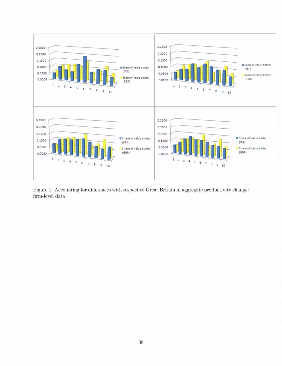
Figure 1: Accounting for di¤erences with respect to Great Britain in aggregate productivity change:�rm-level data
38

Table 1: Time series of the Solow residual
(1) (2) (3) (4) (5)Dep. Variable = log prJt BEL ESP FRA ITA GBRlog prJt�1 0.790*** 0.875*** 0.694*** 0.847*** 0.739***
(0.0957) (0.0973) (0.100) (O.133) (0.0984)N 25 25 25 35 35LM1 (p-value) 0.491 0.926 0.215 0.927 0.396LM3 (p-value) 0.290 0.0166 0.4740 0.992 0.118
The table reports OLS estimates for the years up to 2005. A time trend is included in the regression. LM1 (LM3) is
the Lagrange Multiplier tests for residual serial correlation up to the �rst (third) order. Standard errors are reported
in parentheses. *** signi�cant at less than 0.1 percent; ** signi�cant at 1 percent; * signi�cant at 5 percent.
Table 2: Accounting for aggregate productivity change between 1984 and 2004: aggregate andindustry productivity change (annual rates)
BEL ESP FRA ITA GBRd log pr d log pr d log pr d log pr d log pr-0.0014 -0.0024 0.0076 0.0027 0.0088
Industry:Manufacturing 0.0068 0.0048 0.0112 0.0041 0.0103Electricity, Gas, Water supply 0.0159 0.0327 0.0287 -0.0071 0.0149Construction 0.0100 -0.0091 -0.0034 -0.0120 0.0000Wholesale and Retail -0.0203 -0.0069 0.0065 0.0051 0.0058Finance, Insurance, Real estate 0.0007 -0.0009 -0.0103 -0.0030 -0.0132
Table 3: Accounting for aggregate productivity change between 1998 and 2005: small and large�rms (annual rates)
d log pr(aggregate) group Share(group) d log pr(group)BEL 0.0251 LARGE FIRMS 0.9241 0.0256
SMALL FIRMS 0.0759 0.0182ESP 0.0006 LARGE FIRMS 0.7044 0.0031
SMALL FIRMS 0.2956 -0.0053FRA 0.0293 LARGE FIRMS 0.7964 0.0294
SMALL FIRMS 0.2036 0.0288ITA 0.0057 LARGE FIRMS 0.7019 0.0046
SMALL FIRMS 0.2981 0.0083GBR 0.0523 LARGE FIRMS 0.9417 0.0519
SMALL FIRMS 0.0583 0.0587
39

Table 4: Accounting for di¤erences with respect to Great Britain in aggregate productivity changebetween 1984 and 2003: industry-level data (annual rates)
Tot di¤erence to GBR d log pr Di¤erence accounted by:
di¤erences in average d log pr di¤erences in industrial compBEL -0.0101 -0.0099 -0.0002ESP -0.0112 -0.0117 0.0005FRA -0.0011 0.0005 -0.0017ITA -0.0061 -0.0066 0.0005
40
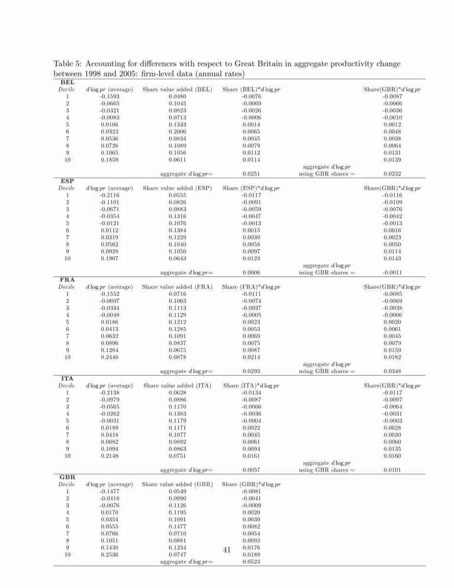
Table 5: Accounting for di¤erences with respect to Great Britain in aggregate productivity changebetween 1998 and 2005: �rm-level data (annual rates)BELDecile d log pr (average) Share value added (BEL) Share (BEL)*d log pr Share(GBR)*d log pr1 -0.1593 0.0480 -0.0076 -0.00872 -0.0665 0.1045 -0.0069 -0.00663 -0.0321 0.0823 -0.0026 -0.00364 -0.0083 0.0713 -0.0006 -0.00105 0.0106 0.1343 0.0014 0.00126 0.0323 0.2006 0.0065 0.00487 0.0536 0.0834 0.0045 0.00388 0.0726 0.1089 0.0079 0.00649 0.1065 0.1056 0.0112 0.013110 0.1859 0.0611 0.0114 0.0139
aggregate d log praggregate d log pr= 0.0251 using GBR shares = 0.0232
ESPDecile d log pr (average) Share value added (ESP) Share (ESP)*d log pr Share(GBR)*d log pr1 -0.2116 0.0555 -0.0117 -0.01162 -0.1101 0.0826 -0.0091 -0.01093 -0.0671 0.0883 -0.0059 -0.00764 -0.0354 0.1316 -0.0047 -0.00425 -0.0121 0.1076 -0.0013 -0.00136 0.0112 0.1384 0.0015 0.00167 0.0319 0.1229 0.0039 0.00238 0.0562 0.1040 0.0058 0.00509 0.0928 0.1050 0.0097 0.011410 0.1907 0.0643 0.0123 0.0143
aggregate d log praggregate d log pr= 0.0006 using GBR shares = -0.0011
FRADecile d log pr (average) Share value added (FRA) Share (FRA)*d log pr Share(GBR)*d log pr1 -0.1552 0.0716 -0.0111 -0.00852 -0.0697 0.1063 -0.0074 -0.00693 -0.0334 0.1113 -0.0037 -0.00384 -0.0048 0.1129 -0.0005 -0.00065 0.0186 0.1212 0.0023 0.00206 0.0413 0.1285 0.0053 0.00617 0.0632 0.1091 0.0069 0.00458 0.0896 0.0837 0.0075 0.00799 0.1284 0.0675 0.0087 0.015910 0.2440 0.0878 0.0214 0.0182
aggregate d log praggregate d log pr= 0.0293 using GBR shares = 0.0348
ITADecile d log pr (average) Share value added (ITA) Share (ITA)*d log pr Share(GBR)*d log pr1 -0.2138 0.0628 -0.0134 -0.01172 -0.0979 0.0886 -0.0087 -0.00973 -0.0565 0.1170 -0.0066 -0.00644 -0.0262 0.1383 -0.0036 -0.00315 -0.0031 0.1179 -0.0004 -0.00036 0.0189 0.1171 0.0022 0.00287 0.0418 0.1077 0.0045 0.00308 0.0682 0.0892 0.0061 0.00609 0.1094 0.0863 0.0094 0.013510 0.2148 0.0751 0.0161 0.0160
aggregate d log praggregate d log pr= 0.0057 using GBR shares = 0.0101
GBRDecile d log pr (average) Share value added (GBR) Share (GBR)*d log pr1 -0.1477 0.0549 -0.00812 -0.0418 0.0990 -0.00413 -0.0076 0.1126 -0.00094 0.0170 0.1195 0.00205 0.0354 0.1091 0.00396 0.0555 0.1477 0.00827 0.0766 0.0710 0.00548 0.1051 0.0881 0.00939 0.1430 0.1234 0.017610 0.2536 0.0747 0.0189
aggregate d log pr= 0.0523
41
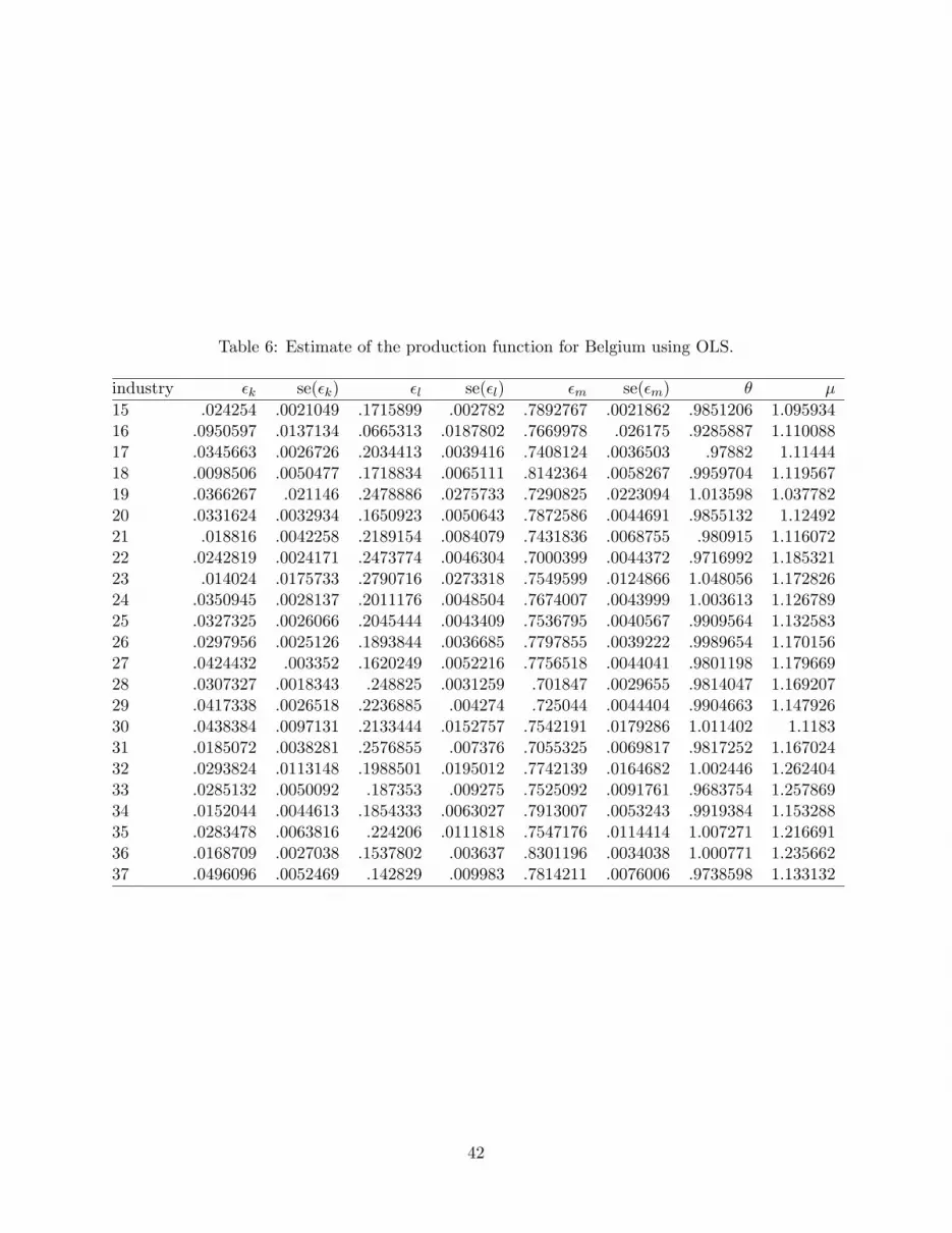
Table 6: Estimate of the production function for Belgium using OLS.
industry �k se(�k) �l se(�l) �m se(�m) � �
15 .024254 .0021049 .1715899 .002782 .7892767 .0021862 .9851206 1.09593416 .0950597 .0137134 .0665313 .0187802 .7669978 .026175 .9285887 1.11008817 .0345663 .0026726 .2034413 .0039416 .7408124 .0036503 .97882 1.1144418 .0098506 .0050477 .1718834 .0065111 .8142364 .0058267 .9959704 1.11956719 .0366267 .021146 .2478886 .0275733 .7290825 .0223094 1.013598 1.03778220 .0331624 .0032934 .1650923 .0050643 .7872586 .0044691 .9855132 1.1249221 .018816 .0042258 .2189154 .0084079 .7431836 .0068755 .980915 1.11607222 .0242819 .0024171 .2473774 .0046304 .7000399 .0044372 .9716992 1.18532123 .014024 .0175733 .2790716 .0273318 .7549599 .0124866 1.048056 1.17282624 .0350945 .0028137 .2011176 .0048504 .7674007 .0043999 1.003613 1.12678925 .0327325 .0026066 .2045444 .0043409 .7536795 .0040567 .9909564 1.13258326 .0297956 .0025126 .1893844 .0036685 .7797855 .0039222 .9989654 1.17015627 .0424432 .003352 .1620249 .0052216 .7756518 .0044041 .9801198 1.17966928 .0307327 .0018343 .248825 .0031259 .701847 .0029655 .9814047 1.16920729 .0417338 .0026518 .2236885 .004274 .725044 .0044404 .9904663 1.14792630 .0438384 .0097131 .2133444 .0152757 .7542191 .0179286 1.011402 1.118331 .0185072 .0038281 .2576855 .007376 .7055325 .0069817 .9817252 1.16702432 .0293824 .0113148 .1988501 .0195012 .7742139 .0164682 1.002446 1.26240433 .0285132 .0050092 .187353 .009275 .7525092 .0091761 .9683754 1.25786934 .0152044 .0044613 .1854333 .0063027 .7913007 .0053243 .9919384 1.15328835 .0283478 .0063816 .224206 .0111818 .7547176 .0114414 1.007271 1.21669136 .0168709 .0027038 .1537802 .003637 .8301196 .0034038 1.000771 1.23566237 .0496096 .0052469 .142829 .009983 .7814211 .0076006 .9738598 1.133132
42

Table 7: Estimate of the production function for Belgium using system GMM (without AR(1)errors)
industry �k se(�k) �l se(�l) �m se(�m) � �
15 .0215719 .0143043 .116369 .0533856 .845057 .0234978 .9829979 1.17338616 .1015663 .0310604 .0631688 .0307818 .7815633 .0627052 .9462985 1.13116917 .0197039 .0122925 .2157265 .0192355 .7701956 .0248191 1.005626 1.15864218 -.0056251 .0206674 .1726151 .035114 .8318266 .0329617 .9988165 1.14375319 .0311772 .0317691 .2345751 .0333582 .7474033 .0138473 1.013156 1.0638620 .0339828 .0176306 .1430129 .0319975 .8317935 .0344319 1.008789 1.18855721 .0109747 .0141275 .2621731 .0495077 .7361645 .0470625 1.009312 1.10553122 -.0020648 .01703 .2060769 .0415456 .7255507 .0572205 .9295627 1.22851623 .0090164 .0240922 .275057 .0588486 .7610017 .0387986 1.045075 1.18221224 -.0025681 .0212298 .2419967 .0459446 .7398928 .0336436 .9793214 1.08639925 .0253915 .0109819 .2186054 .034797 .7245669 .0391779 .9685638 1.08883426 .0415794 .0154214 .1784004 .0352567 .7706105 .0488047 .9905902 1.15638827 .0359403 .0272913 .1275111 .0291271 .7962665 .0325451 .9597178 1.21102128 .0082466 .0110756 .221101 .0223465 .7515167 .0249234 .9808643 1.25195229 .003992 .0129839 .1750448 .0241039 .8069009 .027443 .9859377 1.27752630 .0428727 .0109362 .2259799 .0234276 .7459196 .0248053 1.014772 1.10599531 .0098459 .0318262 .2204551 .0485979 .7511831 .0353373 .9814841 1.24253532 -.0129264 .0155392 .2198884 .0259918 .7900414 .0319096 .9970034 1.28821233 .0143141 .0157171 .2116466 .0439033 .7581939 .0447299 .9841546 1.26737134 .0058168 .0141078 .1667487 .0274858 .8067272 .0201717 .9792928 1.17577235 .0199072 .0128357 .1912204 .0391206 .7724271 .0389743 .9835548 1.2452436 -.0145004 .0134578 .1721131 .0259554 .8601587 .0200723 1.017771 1.28037737 .0538229 .0186533 .1383617 .0440445 .7744551 .0277837 .9666397 1.123031
43

Table 8: Estimate of the production function for Belgium using system GMM (without AR(1)errors): validating tests
industry hansen (p-value) ar1 (p-value) ar2p (p-value)15 .1526701 2.48e-08 .225985916 1 .1564406 .795462317 .0493479 .0102783 .08024218 .7306365 .0457279 .691472519 1 .9864044 .079671820 .6683506 .001477 .08991721 .2565103 .0130565 .629699122 .1097888 .0124187 .932118723 1 .8665326 .152677424 .6437734 .0004697 .108511625 .5183361 .0621041 .238814526 .1234163 .0059662 .43726827 .605441 .0003418 .304629528 .0032045 .0080472 .442416629 .0916351 .0000682 .525880630 1 .3186199 .207430331 .1405106 .0128848 .806611832 .9991825 .4230046 .096840633 .853533 .0147613 .664702834 .2278766 .0112883 .465557435 .9994887 .0619346 .150975236 .956588 .0000944 .248651837 .6836056 .054695 .4062182
44

Table 9: Estimate of the production function for Belgium using Olley Pakes.
industry �k �l �m � �
15 .0053129 .1607034 .7857859 .9518021 1.09108716 .006006 .0524176 .7730815 .8315051 1.11889317 .0042158 .195162 .737206 .9365838 1.10901418 .0054147 .1729344 .8007517 .9791009 1.10102619 .0053613 .2503178 .7430528 .9987319 1.05766820 .0111285 .1595692 .7815555 .9522532 1.11677121 .0111529 .2168774 .7270212 .9550515 1.091822 .0097333 .2480117 .6909198 .9486648 1.16987823 .0099718 .281923 .7470524 1.038947 1.16054224 .0110562 .1813903 .766848 .9592946 1.12597825 .0110247 .1982173 .7443261 .9535682 1.11852726 .0143439 .189329 .757315 .9609879 1.13643727 .0138856 .1633305 .7672731 .9444892 1.16692628 .0129493 .2405701 .6961676 .949687 1.15974629 .0136856 .2278383 .7157144 .9572383 1.13315530 .0138737 .2379677 .7353308 .9871722 1.09029431 .0145976 .2384386 .6918178 .944854 1.14433932 .0144183 .2252213 .7305138 .9701534 1.19114933 .0147442 .1848012 .7544926 .9540381 1.26118434 .0146547 .1883912 .7944484 .9974943 1.15787635 .0152902 .2039668 .7447227 .9639798 1.20057836 .0152605 .1524164 .8277795 .9954565 1.23217937 .0156083 .1322395 .7942417 .9420895 1.151723
Table 10: Decomposition of the change in aggregate productivity (estimates using System GMMwithout AR(1) errors)
country d logpr (�� 1)(d logX + d logM=Q) R� +RM d log T ResidualBEL .0352278 0.01446 0.00048 .0114122 0.00888ESP .0311934 0.02011 -0.00132 .0048491 0.00755FRA .0478567 -0.00055 0.00169 .0405101 0.00621GBR .0601621 -0.00084 0.00083 .0490316 0.01114ITA .0280874 0.00695 0.00025 .0141505 0.00674
Notes: The estimates of �rm productivity are obtained by estimating a production function with year �xed e¤ects
using system GMM.
45
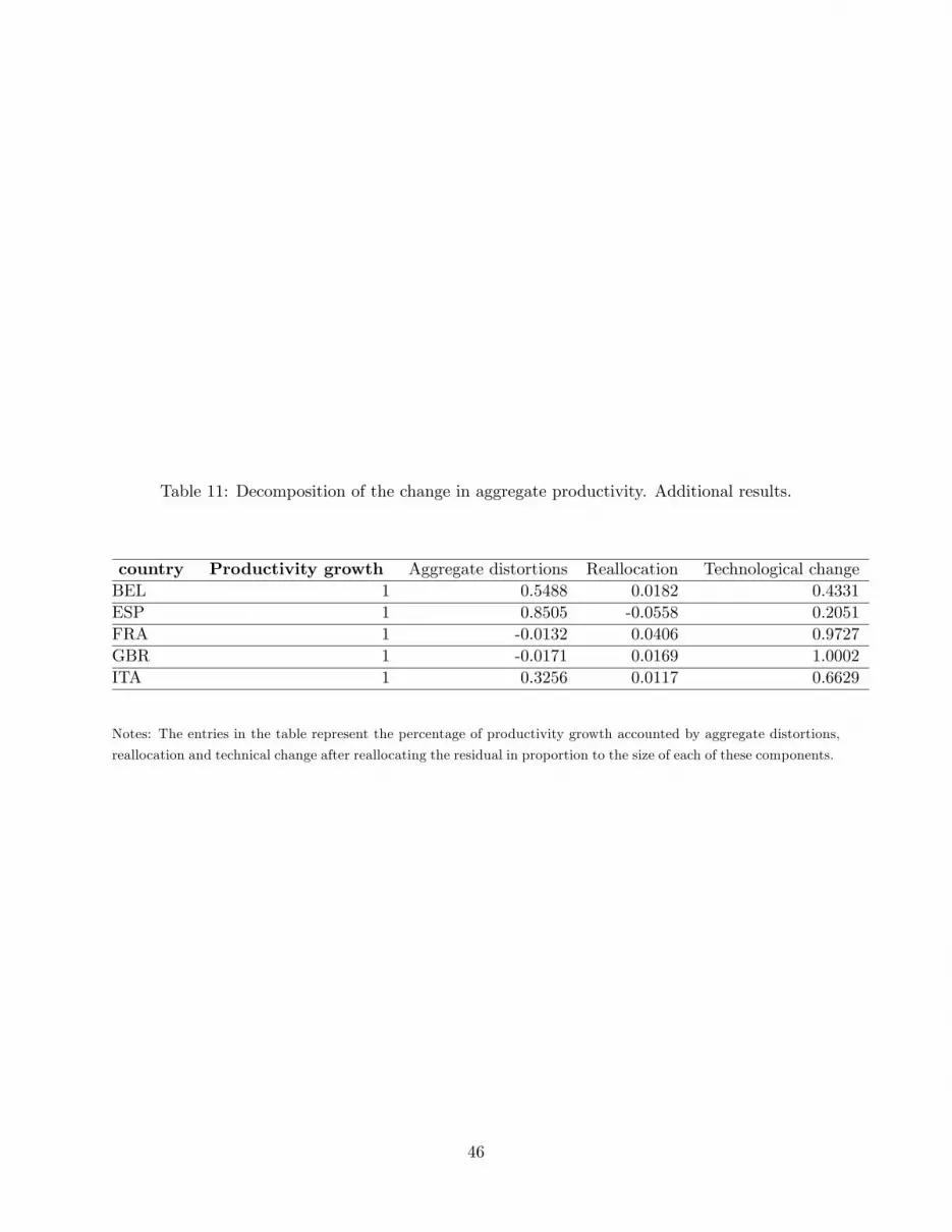
Table 11: Decomposition of the change in aggregate productivity. Additional results.
country Productivity growth Aggregate distortions Reallocation Technological changeBEL 1 0.5488 0.0182 0.4331ESP 1 0.8505 -0.0558 0.2051FRA 1 -0.0132 0.0406 0.9727GBR 1 -0.0171 0.0169 1.0002ITA 1 0.3256 0.0117 0.6629
Notes: The entries in the table represent the percentage of productivity growth accounted by aggregate distortions,
reallocation and technical change after reallocating the residual in proportion to the size of each of these components.
46