Trade Liberalization and the Great Labor Reallocation∗

Yuan Zi†

May 17, 2021

Abstract

What is the role of migration frictions in shaping the effects of trade policy? I address

this question by analyzing the impact of tariff reductions on the spatial allocation of labor in

China and how this impact depends on migration frictions that stem from China’s household

registration system (hukou). I first provide reduced-form evidence that trade liberalization has

induced significant spatial labor reallocation in China, with a stronger effect in regions with

less hukou frictions. I show that the standard quantitative spatial models, by design, would

imply that the gains from trade are largely irrelevant to factor market reforms. A more realistic

calibration suggests that trade liberalization increases China’s welfare by 0.72%, a sizable share

of which comes from mitigating the cost of domestic frictions: if China first abolishes the hukou

system, the gains from tariff reductions would decrease by 15%, and its negative distributional

consequences would be greatly amplified. In contrast, a standard spatial model suggests that

hukou abolition increases the gains from tariff reductions by 1% and alleviates its negative

distributional consequences.

JEL Classification: F14, F15, F16

Keywords: trade liberalization, spatial labor reallocation, hukou frictions

∗First draft: March 2015. I am grateful to Richard Baldwin, Nicolas Berman, Arnaud Costinot, Rodrigo Adao,Pol Antras, David Autor, Andy Bernard, Tibor Besedes, Loren Brandt, Lorenzo Caliendo, Kerem Cosar, David Dorn,Peter Egger, Aksel Erbahar, Benjamin Faber, Luisa Gagliardi, Gordon Hanson, Beata Javorcik, Ruixue Jia, VictorKummritz, Justin Yi Lu, Enrico Moretti, Andreas Moxnes, Rahul Mukherjee, Marc Muendler, Marcelo Olarreaga,Ugo Panizza, Frederic Robert-Nicoud, Stela Rubinova, Kjetil Storesletten, Lore Vandewalle, Johanna Vogel, YikaiWang, Zi Wang, Shang-Jin Wei and Xing Yang for their valuable comments and suggestions at various stages of thedevelopment of this paper. I also thank the Economics faculty of the Massachusetts Institute of Technology (MIT) fortheir hospitality during my visit as a doctoral researcher, as well as the Sociology Department of Peking Universityand Renmin University of China for providing me access to part of the data. This project has received funding fromthe European Research Council under the European Union’s Horizon 2020 research and innovation program (grantagreement 715147).†University of Zurich, Zurich, Switzerland. Email: yuanzi.economics@gmail.com.

1

1 Introduction

Trade liberalization is often argued to be an important driver of economic development because it

can raise a country’s income by increasing specialization, providing access to cheap foreign inputs,

and facilitating the adoption of new technologies. Prominent trade theories typically focus on long-

run equilibrium, assuming that the reallocation of resources across economic activities is frictionless.

However, in reality, factor adjustments tend to be slow, costly, and heterogeneous across space. In

particular, there is increasing evidence that labor immobility can explain a considerable share of

the negative consequences of trade on labor market outcomes.1 Although the role of role of labor

mobility in shaping the impacts of trade has long been emphasized, we lack a rigorous understanding

of how globalization affects a country’s internal labor adjustments and how migration frictions shape

the general equilibrium impact of tariff reductions.

In this paper, I exploit China’s liberalization episode after its accession to the WTO and the

country’s unique household registration system (hukou) to make three contributions to our un-

derstanding of the interaction between trade and migration frictions. First, I provide empirical

evidence of trade-induced spatial labor reallocation and the presence of migration frictions caused

by the hukou system. Second, I show that the standard quantitative spatial model by design implies

that the gains from trade are independent of factor market distortions. In other words, the sur-

prisingly weak complementary found between goods and factor market liberalization found in the

quantitative literature is a consequence of specific model assumptions, rather than an informative

result from the data. Finally, I quantify the impact of tariff reductions and its interaction with

domestic hukou reforms using a more realistic calibration, where the opposite results emerge from

those of the standard model.

China offers a particularly suitable setting to study this subject for three reasons. First, the

composition of industries differs significantly across Chinese prefectures, providing ample variation

to identify the causal effects of trade policy on regional economic outcomes. Second, although trade

has been growing rapidly in China, the country’s accession to the WTO was an inflection point:

China’s total trade in goods was approximately one-half trillion USD in 2000, and it had surged to

more than 4 trillion USD by the end of 2010. In the same period, China’s internal migration also

accelerated. From 1995 to 2000, approximately thirty million Chinese changed their province of

residence. This number increased to nearly fifty million between 2000 and 2005 and further reached

sixty million by 2010.2 This rapid increase in internal migration is largely a consequence of workers

moving from inland areas to coastal cities, which contributed the most to China’s trade surge over

the same period, making it a natural choice to probe the relationship between international trade

1See, for instance, Autor et al. (2013), Topalova (2010), and Dix-Carneiro and Kovak (2017) for the cases of theUS, India, and Brazil, respectively.

2The numbers are calculated based on the 2000 and 2010 rounds of the population census and the 2005 round ofthe 1% population sampling survey.

2

and domestic migration patterns.

Importantly, unlike most policies that tend to affect the movement of both goods and people,

China’s hukou system offers a unique possibility to cleanly identify migration frictions separate from

other types of domestic frictions. Introduced in the 1950s, the system has long been recognized as

the most important factor restricting internal mobility in China. It ties a person’s access to various

social benefits and public services to her residential status; as a result, the ease of obtaining a

hukou substantially influences one’s migration decisions. Notably, the stringency of the hukou

system differs across provinces. This spatial heterogeneity provides an ideal setting for identifying

the role of migration frictions in shaping the impact of trade on regional labor market outcomes.

Drawing on a rich dataset I assembled on China’s regional economy, I first empirically document

the trade-induced labor reallocation across Chinese prefectures and the presence of hukou frictions.

To this end, I develop a novel measure of migration frictions associated with the hukou system based

on the hukou-granting probability of each region. Exploiting regional variations in the exposure to

tariff changes, I find that among various trade shocks associated with China’s accession to the

WTO, input tariff liberalization played a dominant role in shaping the spatial labor reallocation.3

In provinces with the least hukou frictions, the effect of input tariff cuts was three times larger

than the average effect. When accounting for both the input and output channels, 29 percent of

the regional variation in employment changes can be attributed to trade liberalization. Regional

adjustments on other margins suggest that the observed regional employment changes were mainly

driven by interregional labor adjustments and confirm the existence of hukou frictions. The results

are robust to various instrumenting strategies and placebo tests and to correcting standard errors to

account for spatial correlations, skill heterogeneity across workers, concurrent economic shocks and

policy changes including hukou reforms. I also provide a battery of robustness checks and placebo

tests to the hukou measure, showing that its value is not driven by the composition of migration

inflows, demand factors, or unobserved heterogeneity. The baseline results are also robust when we

consider various alternative hukou measures.

Next, I interpret the empirical results through the lens of a quantitative spatial model. For this

purpose, I extend the theoretical framework of Redding (2016) to explicitly model input-output

linkages and hukou frictions. More important, I relax the Cobb-Douglas assumption to allow for

more realistic substitution between and across factors, intermediate inputs, and primary factors in

production and consumption across industries. While the quantitative framework can be enriched

in various ways, deviating from a unitary elasticity of substitution is the key to quantify how gains

from trade depend on factor market distortions. The key is to recognize that the Cobb-Douglas

production function is special. Its whole input-output matrix is constant and can be taken as

exogenous. In this case, the Hulten theorem (Hulten 1978) is globally exact, namely for efficient

economies, the impact on aggregate welfare of a microeconomic technology shock is equal to the

3Throughout the empirical analysis, I control for output tariff cuts, external tariff changes and their interactionswith the hukou friction measure (among others) and do not find robust evidence of their impacts on migration.

3

shocked industry’s production shares. As a result, the microeconomic details of the production

structure are irrelevant (Baqaee and Farhi, 2019b).

By acknowledging this insight and applying it to the spatial setting, I am able to explain two

puzzles associated with the standard spatial quantitative models. First, these models are usually

surprisingly sticky, predicting nearly zero interaction effect between trade and various types of factor

market frictions.4 Intuitively, as the microeconomic details do not matter, the aggregate gains from

trade will not be affected by the extent of factor allocation. Second and relatedly, how domestic

friction shapes the distributional effect of trade is completely governed by the reallocation term,

which always implies a dampened regional variation in gains from trade when factors become more

mobile. These knife-edge properties disappear once one deviates from Cobb-Douglas, and then

the whole production structure responds endogenously to shocks, and resulting nonlinearities are

shaped by microeconomic details.

I proceed by calibrating the model to identify the general equilibrium effects of tariff reductions

and quantify the importance of hukou frictions. I do so with 30 Chinese provinces and a constructed

rest of the world. The simulated regional employment changes qualitatively match well with the

observed data. I find that trade liberalization increases China’s welfare by 0.72%. However, the

welfare gains are not shared equally across provinces. Individuals with Beijing and Shanghai hukou

experience welfare improvements of 1.88% and 1.59%, while individuals who hold a hukou from

Gansu or Shannxi provinces gain only 0.38% and 0.41%, respectively. Overall, trade liberalization

amplifies regional inequalities in China.

I further assess the extent to which China would have gained from trade liberalization if the

hukou system had been abolished. To this end, I first quantify the cost of the hukou system. I find

that in a province with median hukou frictions, migrant workers are willing to forgo 17% of their

income to obtain a local hukou. Abolishing the hukou system improves aggregate welfare by 1.34%

and alleviates regional disparities in China, although in regions such as Beijing and Shanghai, hukou

holders experience welfare losses. Starting from this new equilibrium, the aggregate gains from the

same tariff reductions would decrease by 15% relative to the case with hukou frictions, suggesting

that a sizable share of the gains from trade in the old equilibrium actually comes from mitigating the

cost of domestic frictions. This results suggest that trade and free factor allocation are substitutes,

broadly consistent with the insight dating back to Chipman (1969), Deardorff (1994) and Hanson

and Slaughter (1999), among others. The gains from tariff reduction also become more unevenly

spatially distributed without hukou frictions. In sharp contrast, the standard spatial model with

Cobb-Douglas production suggests that hukou abolition increases gains from tariff reductions by

1% and weakly alleviates its negative distributional outcomes.

This paper contributes to a rich empirical literature on trade and local labor markets. Autor

et al. (2016) provide a thorough survey of the existing literature. Unlike most of the work focusing

4For example between domestic geography and trade in Fan (2015), between commuting costs and trade liberal-ization in Monte et al. (2015), and between factor misallocation and trade shocks in Ouyang (2021), amongst others.

4

on the downsides of increased import competition (Autor et al. (2013), Dauth et al. (2014), Dix-

Carneiro and Kovak (2017), Kovak (2011, 2013), McLaren and Hakobyan (2010) and Topalova

(2007, 2010), Facchini et al. (2017), among others),5 I highlight the positive impact of input trade

liberalization and emphasize the importance of migration frictions in shaping the impact of trade

policy. Relatedly, Goldberg and Pavcnik (2007b) and Topalova (2007) find that the poor are more

likely to share in the gains from trade liberalization in regions with flexible labor markets. In terms

of focus, my paper also broadly connects to the large literature on trade and labor allocation in

less-developed countries (see Goldberg and Pavcnik (2007a) and Harrison et al. (2011) for surveys)

and on trade and costly labor adjustments. Examples include Kambourov (2009), Artuc et al.

(2010), Artuc and McLaren (2012), Caliendo et al. (2015), Dix-Carneiro (2014), and many others

(see McLaren (2017) for a recent review).

In terms of modeling techniques, this paper closely follows a growing literature that develops

spatial general equilibrium models to analyze the welfare consequences of aggregate shocks while ac-

counting for trade and mobility frictions within countries (for example, Caliendo et al. (2015), Galle

et al. (2017), Monte et al. (2015), Redding (2016) and Bryan and Morten (2017)). Important works

in the Chinese context include Tombe and Zhu (2019) on quantifying the aggregate productivity

increases due to trade and migration reductions and Fan (2015) on how domestic geography and

trade affect skill premiums.6 I contribute to the literature by introducing the insight of Baqaee and

Farhi (2019b) and show that it is crucial to deviate from Cobb-Douglas to quantify the interaction

effect between trade policy and geography. By examining real-world trade liberalization, I am also

able to guide and cross-validate my model construction with credibly identified empirical evidence.

In this sense, my paper is closely related to Caliendo et al. (2017), who quantify the effect of trade

and labor market integration due to EU enlargement by exploiting the observed changes in tariffs

and migration policies.

The remainder of this paper is organized as follows. In the next section, I describe the empirical

context, discuss the data, and present the empirical results. Section 3 presents the theoretical

framework. In Section 4, I estimate and calibrate the key parameters of the model, quantify the

effects of tariff reductions, and explore a counterfactual scenario in which the hukou system is

abolished. Section 5 concludes the paper.

5An exception is Dauth et al. (2014), who find that the rise of China and Eastern Europe caused substantial joblosses in regions in Germany that specialized in import-competing industries but job gains in regions specialized inexport-oriented industries.

6Other works studying the interaction between trade and domestic geography include Cosar and Fajgelbaum (2013)and Fajgelbaum and Redding (2014), who show that the difference in domestic trade costs to international gates canlead to heterogeneous regional development after external integration; Monte et al. (2015) emphasize the role ofcommuting ties to estimate local employment elasticities, and Ramondo et al. (2016) find that domestic trade costsare substantial impediments to scale effects.

5

2 Input Liberalization and Regional Hukou Frictions

In this section, I explain the history of trade reforms and the hukou system in China, describe the

data and measurements, and present four empirical patterns that demonstrate input-liberalization-

induced spatial labor adjustments and the presence of hukou frictions.

2.1 Empirical Context

China’s Trade Liberalization

Prior to the economic reforms of the early 1980s, the average tariff level in China was 56%.7 This

tariff schedule was introduced in 1950 and went nearly unchanged in subsequent decades, partly

due to the relative unimportance of trade policy in a centrally planned economy.8 Starting in 1982,

China engaged in a series of voluntary tariff cuts, driving down the simple average tariffs to 24% in

1996 (Li, 2013). However, the government also introduced pervasive and complex trade controls in

the same period – import quotas, licenses, designated trading practices and other non-tariff barriers

were widely used (Blancher and Rumbaugh, 2004). In addition, the Chinese RMB depreciated by

more than 60% in the 1980s and by a further 44% in 1994 to help firms export (Li, 2013).9 As a

result, changes in tariff duties reflect neither the changes in the actual protection faced by Chinese

firms nor the accessibility of imported inputs.

In 1996, to meet the preconditions for WTO accession, the Chinese government engaged in

substantial reforms that did away with most of the restrictive non-tariff barriers. Trade licenses,

special import arrangements, and discriminatory policies against foreign goods were reduced or

eliminated to make tariffs the primary instruments of protection.10 Phased tariff reductions started

in 2001. In 2000, China’s simple average applied tariff was 17%, with the standard deviation across

the six-digit Harmonized System (HS6) products being 12%. By the end of 2005, the average

tariff level was reduced to 6%, and the standard deviation almost halved. The average tariff level

stabilized after 2005.11 Thus, I measure trade liberalization based on the change in tariff rates

7This is the 1982 unweighted average tariff documented by Blancher and Rumbaugh (2004).8Under the planned economy, import and export quantities were government decisions rather than reflections of

market supply and demand (Ianchovichina and Martin, 2001). During this period, trade in China was run by 10 to16 foreign-trade corporations who were de facto monopolies in their specified product ranges (Lardy, 1991).

9There was also substantial tariff redundancy resulting from various preferential arrangements, for example, importsfor processing purposes, for military uses, to Special Economic Zones and to certain areas near the Chinese borderwere subject to waivers or reductions in import duties. According to Ianchovichina and Martin (2001), only 40% ofimports were subject to official tariffs.

10The share of imports subject to licensing requirements fell from a peak of 46% in the late 1980s to less than 4%of all commodities by the time China entered the WTO. The state abolished import substitution lists and authorizedtens of thousands of companies to engage in foreign trade transactions, undermining the monopoly powers of statetrading companies. The transformation was similarly far-reaching on the export side (Lardy, 2005). The duty-freepolicy on imports for personal use in Special Economic Zones was gradually abolished in the 1990s; the preferentialduty in Tibet was abolished in 2001. Moreover, China also abolished, modified or added over a thousand nationalregulations and policies. At the regional level, more than three thousand administrative regulations, and over 188,000policy measures implemented by provincial and municipal governments were stopped (Li, 2011).

11All numbers are calculated using the simple average of Most Favored Nation (MFN) applied tariffs at the HS6

6

between 2000 and 2005.

The Hukou System

A hukou is a household registration record that officially identifies a person as a resident of an

area in China and determines where citizens are officially allowed to live. The hukou system was

introduced in the early 1950s to harmonize the old household registration systems across regions,

but it was soon re-purposed to restrict both interregional and rural-to-urban migration.12 At the

beginning of the 1960s, free migration had become extremely rare. Migrant workers required six

passes to work in provinces other than their own; rural-to-urban migrants, in addition to the above

restrictions, would have to first acquire an urban hukou, the annual quota of which was 0.15% to

0.2% of the non-agricultural population of each locale (Cheng, 2007). Under the central planning

system, coupons for consumption goods, employment and other resources were allocated entirely

based on local hukou; urban dwellers without local hukou would be fined, arrested and deported.

These practices made it impossible for people to work and live outside their authorized domain

(Cheng and Selden, 1994).

In the early 1980s, China latched onto a labor-intensive, export-oriented development strategy

that created an increasingly large labor demand in cities. In 1984, the State Council allowed rural

populations to reside in villages with self-sustained staples, and migration policy then began to relax

over time.13 The distinction between rural and urban hukou also gradually became less important

(Bosker et al., 2012) and the rural-to-urban migration quotas were officially abolished in 1997 (Chan,

2009). Nevertheless, the hukou system continues to serve as the primary instrument for regulating

interregional migration. As cheap labor continues to flood the labor market, in the absence of related

fiscal transfers, local governments in general have very little incentive to provide public services to

migrant workers. Individuals who do not have a local hukou in the place where they live are not

able to access certain jobs, schooling, subsidized housing, healthcare and other benefits enjoyed by

those who do. As a result, the ease of obtaining a local hukou still heavily influences one’s migration

decisions.

Importantly, as part of a contemporaneous reform devolving fiscal and administrative powers

to lower-level governments, local governments have largely gained the authority to determine the

number of hukou to issue in their jurisdictions. In 1992, some provinces began to offer temporary

level from the United Nations’ (UN) Trade Analysis Information System (TRAINS).12The uneven allocation of resources under the centrally planned economy led to a massive influx of migrants into

cities, threatening agricultural production in rural areas (Kinnan et al., 2015). In response, the Chinese governmentbegan to tighten migration controls. In 1958, the Standing Committee of the National People’s Congress adoptedthe Household Registration Regulations. According to these regulations, citizens could only apply to move after theregistration authority had granted their local hukou. China then entered an era with strict migration controls, withthe hukou being at the center of the migration control system. The details of this policy change are provided in section2.5, when discussing the hukou instrument.

13In the following year, the Ministry of Public Security of China allowed people to migrate freely conditional onapplying for a temporary residential permit upon arrival. In 1993, China officially ended the food rationing system,and internal migration was thus no longer limited by hukou-based consumption coupons.

7

resident permits for anyone who has a legitimate job or business in one of their major cities, and

some grant hukou to high-skilled professionals or businessmen who make large investments in their

region (Kinnan et al., 2015). The stringency of these policies and general hukou issuing rules,

however, differ significantly across regions. For instance, it is famously difficult to obtain a hukou

in Beijing or Shanghai, while Henan is relatively generous in granting local hukou to migrants. This

heterogeneity provides spatial variation that I exploit with the hukou friction measure.

2.2 Data and Measurement

To evaluate the impact of tariff reductions on regional economies in China, I construct a panel

dataset of 337 Chinese prefecture-level divisions (prefectures for short). The core data track pre-

fectures decennially from 2000-2010, with the 1990 value being available for some variables. Table

1 contains descriptive statistics of the main variables that are used in Section 2, which I describe

throughout this section. I provide a more detailed discussion of the data construction and the other

variables used in the paper in Appendix A.14

Local Labor Markets

Throughout the empirical analysis, local labor markets are defined as prefectures. A prefecture

is an administrative division of China that ranks below a province and above a county. As the

majority of regional policies, including the overall planning of public transportation, are conducted

at the prefecture level (Xue and Zhang, 2001), I expect counties within the same prefecture to

have strong commuting ties and be economically integrated, and thus Chinese prefectures serve as

a good proxy for commuting zones. To account for prefecture boundary changes, I use information

on the administrative division changes published by the Ministry of Civil Affairs of China to create

time-consistent county groups based on prefecture boundaries in the year 2000. This results in

337 geographic units that I refer to as prefectures or regions, including four directly controlled

municipalities and 333 prefecture-level divisions that cover all of mainland China. Compared to

the commuting zones in the United States, the Chinese prefectures are approximately twice the

size on average and 1.5 times the size when the 10 largest (but sparsely populated) prefectures in

autonomous regions are excluded.

The empirical analysis in this paper studies 10-year changes in prefecture employment, total

and working age populations, the most recent five-year migrant inflows from other provinces, and

the population holding local hukou in each prefecture. I collect these variables at the county level

from the Tabulation of Population Census of China by County for the years 2000 and 2010 and then

aggregate them to prefectures based on the time-consistent county groups. Notably, the employment

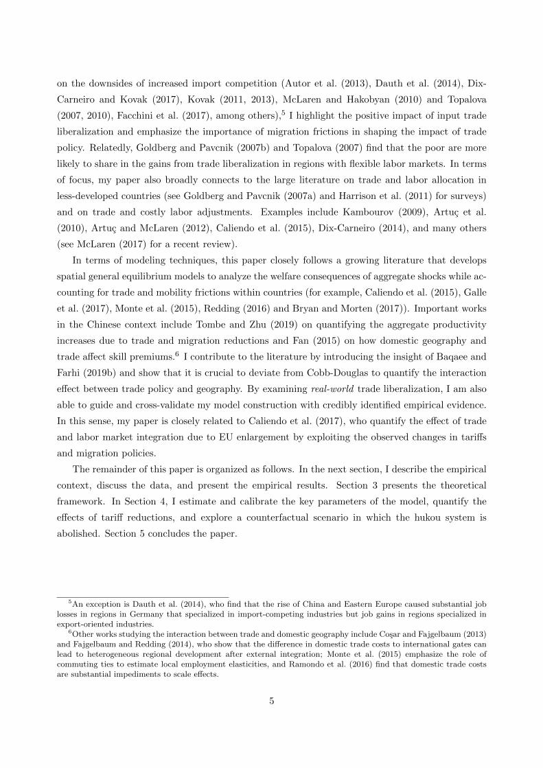
measure includes informal workers, the lion’s share of which are migrants.15 Figure 1 shows the

14One data contribution of the paper is to consolidate 16 datasets (including different publications of the Chinesepopulation census) and to create crosswalks that are consistent across various data sources.

15According to Park et al. (2012), informal employment in China is defined either based on (i) whether the employer

8

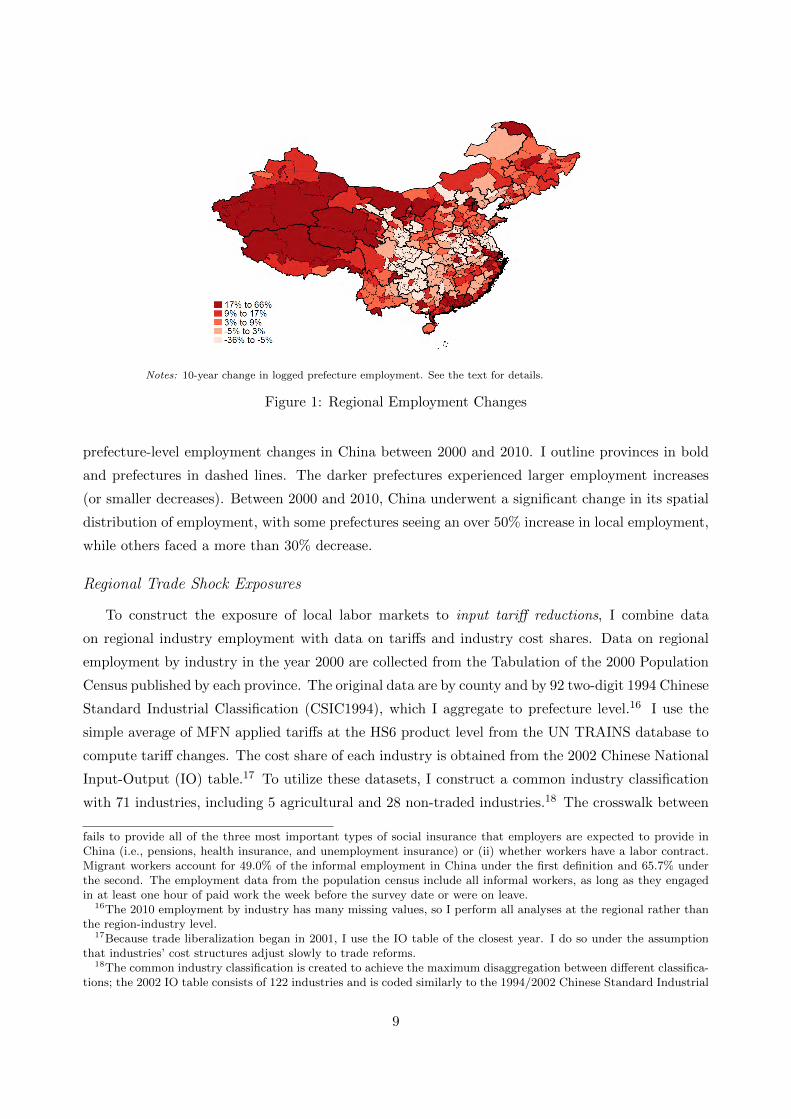
Notes: 10-year change in logged prefecture employment. See the text for details.

Figure 1: Regional Employment Changes

prefecture-level employment changes in China between 2000 and 2010. I outline provinces in bold

and prefectures in dashed lines. The darker prefectures experienced larger employment increases

(or smaller decreases). Between 2000 and 2010, China underwent a significant change in its spatial

distribution of employment, with some prefectures seeing an over 50% increase in local employment,

while others faced a more than 30% decrease.

Regional Trade Shock Exposures

To construct the exposure of local labor markets to input tariff reductions, I combine data

on regional industry employment with data on tariffs and industry cost shares. Data on regional

employment by industry in the year 2000 are collected from the Tabulation of the 2000 Population

Census published by each province. The original data are by county and by 92 two-digit 1994 Chinese

Standard Industrial Classification (CSIC1994), which I aggregate to prefecture level.16 I use the

simple average of MFN applied tariffs at the HS6 product level from the UN TRAINS database to

compute tariff changes. The cost share of each industry is obtained from the 2002 Chinese National

Input-Output (IO) table.17 To utilize these datasets, I construct a common industry classification

with 71 industries, including 5 agricultural and 28 non-traded industries.18 The crosswalk between

fails to provide all of the three most important types of social insurance that employers are expected to provide inChina (i.e., pensions, health insurance, and unemployment insurance) or (ii) whether workers have a labor contract.Migrant workers account for 49.0% of the informal employment in China under the first definition and 65.7% underthe second. The employment data from the population census include all informal workers, as long as they engagedin at least one hour of paid work the week before the survey date or were on leave.

16The 2010 employment by industry has many missing values, so I perform all analyses at the regional rather thanthe region-industry level.

17Because trade liberalization began in 2001, I use the IO table of the closest year. I do so under the assumptionthat industries’ cost structures adjust slowly to trade reforms.

18The common industry classification is created to achieve the maximum disaggregation between different classifica-tions; the 2002 IO table consists of 122 industries and is coded similarly to the 1994/2002 Chinese Standard Industrial

9

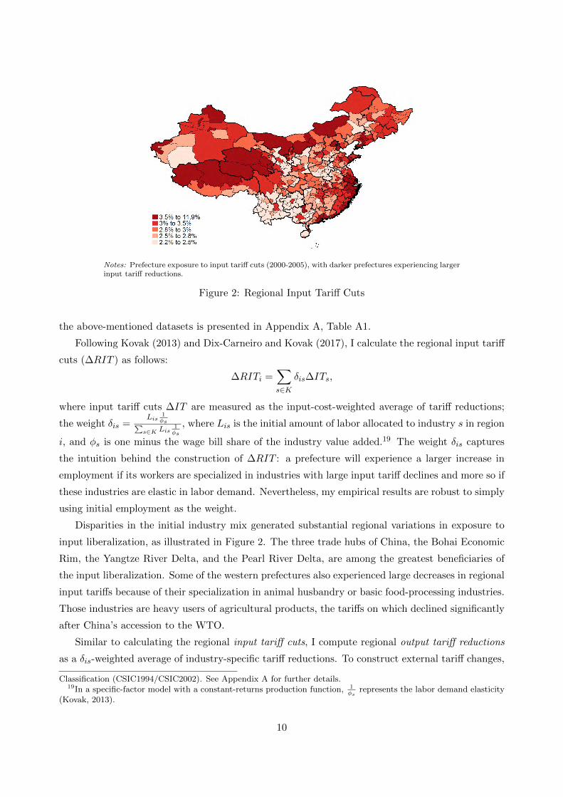
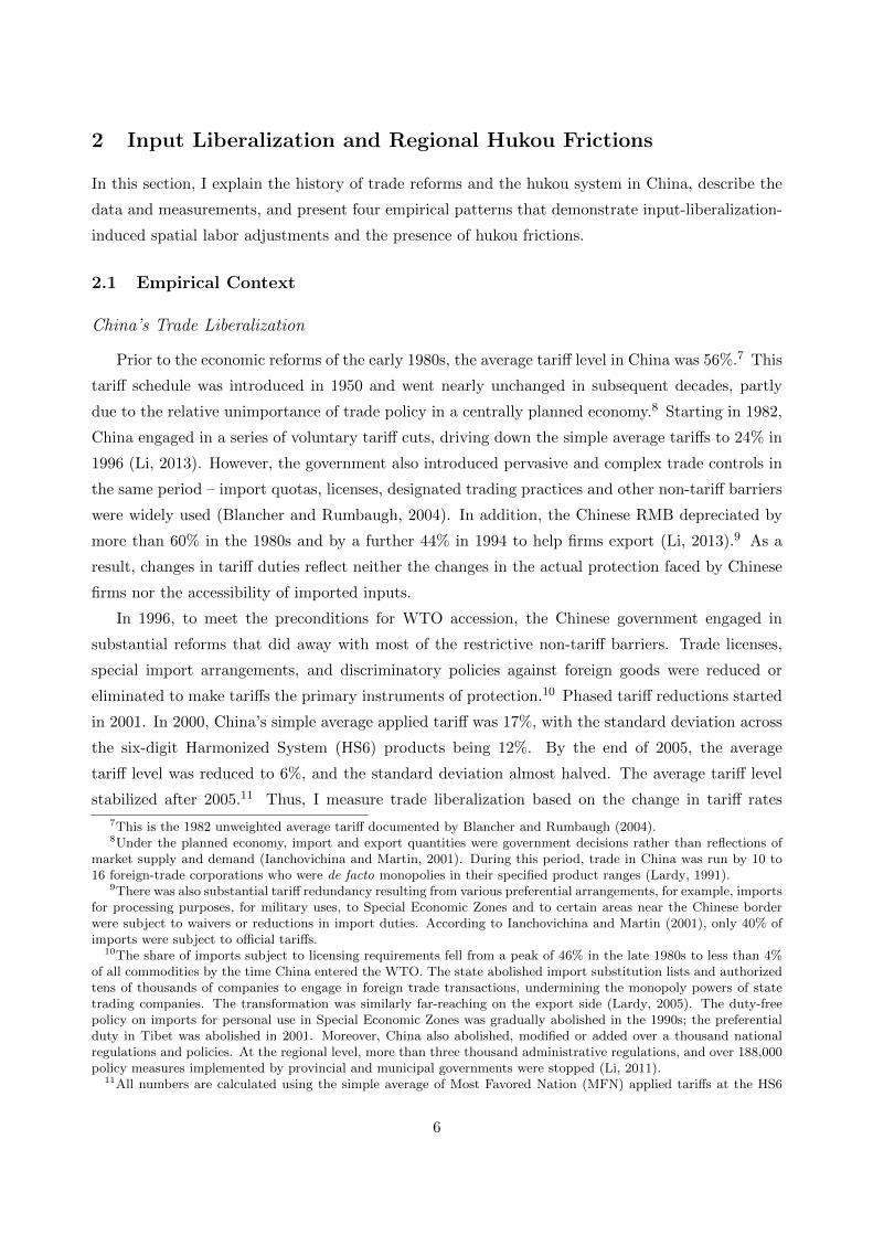
Notes: Prefecture exposure to input tariff cuts (2000-2005), with darker prefectures experiencing largerinput tariff reductions.

Figure 2: Regional Input Tariff Cuts

the above-mentioned datasets is presented in Appendix A, Table A1.

Following Kovak (2013) and Dix-Carneiro and Kovak (2017), I calculate the regional input tariff

cuts (∆RIT ) as follows:

∆RITi =∑s∈K

δis∆ITs,

where input tariff cuts ∆IT are measured as the input-cost-weighted average of tariff reductions;

the weight δis =Lis

1φs∑

s∈K Lis1φs

, where Lis is the initial amount of labor allocated to industry s in region

i, and φs is one minus the wage bill share of the industry value added.19 The weight δis captures

the intuition behind the construction of ∆RIT : a prefecture will experience a larger increase in

employment if its workers are specialized in industries with large input tariff declines and more so if

these industries are elastic in labor demand. Nevertheless, my empirical results are robust to simply

using initial employment as the weight.

Disparities in the initial industry mix generated substantial regional variations in exposure to

input liberalization, as illustrated in Figure 2. The three trade hubs of China, the Bohai Economic

Rim, the Yangtze River Delta, and the Pearl River Delta, are among the greatest beneficiaries of

the input liberalization. Some of the western prefectures also experienced large decreases in regional

input tariffs because of their specialization in animal husbandry or basic food-processing industries.

Those industries are heavy users of agricultural products, the tariffs on which declined significantly

after China’s accession to the WTO.

Similar to calculating the regional input tariff cuts, I compute regional output tariff reductions

as a δis-weighted average of industry-specific tariff reductions. To construct external tariff changes,

Classification (CSIC1994/CSIC2002). See Appendix A for further details.19In a specific-factor model with a constant-returns production function, 1

φsrepresents the labor demand elasticity

(Kovak, 2013).

10

I first use the Chinese customs data for 2000 to compute prefecture exports and calculate the

export share by destination country for each industry and prefecture. I then take the export-

share-weighted average of the tariff changes across destination countries over the 2000-2010 period

to obtain prefecture-industry-specific tariff reductions. In the last step, I compute the weighted-

average tariff changes across industries using δis for each prefecture. Table A2 provides descriptive

statistics of these variables.

Relevance of Trade Flows

Before analyzing the impact of input tariff reductions on regional employment and migration, I

first provide evidence that input liberalization indeed had a positive impact on trade flows at both

the industry and regional levels. I employ Chinese firm-level customs data to exclude processing

imports, as they are exempt from tariffs.20 Table A3 presents the estimation results. Guided

by Goldberg et al. (2010), I begin by examining the responsiveness of import values to tariffs by

regressing the logged import value of an HS6 product on Chinese tariffs at the same level, controlling

for product and year fixed effects.21 Table A3, columns (1) and (2) of panel (a) report the coefficient

estimates on tariffs for all products and for intermediates, respectively. In both cases, declines in

tariffs were associated with higher imported values. In columns (3) and (4), I explore the impact

of tariff reductions on unit values of HS6-country varieties by regressing the unit value of the HS6-

country product on the tariff, a year fixed effect, and an HS6-country fixed effect. I find that lower

tariffs were associated with declines in the unit value of existing intermediate imports. Finally, I

explore the impact of tariff reductions on the expansion of imported varieties, with a variety being

defined as an HS6-country-specific product. As shown in columns (5) and (6), tariff declines were

associated with increases in imported varieties. In panel (b), I examine the regional correlations.

In columns (1) and (2), I explore the correlation between prefecture-level import changes and

regional input tariff cuts; columns (3) and (4) examine the responsiveness of imported varieties. In

all regressions, I control for external tariff reductions, output tariff reductions, and province fixed

effects. I find that larger regional input tariff cuts were associated with a greater increase in regional

imports and imported varieties, and the results are robust when focusing on intermediates.

The Hukou Measure

The primary dataset that I use to construct the hukou measure is the 0.095% random-sampled

microdata of the Population Census in 2000. The sample was drawn at the household level, with

a unique identifier linking individuals in the same household. It contains rich individual-level in-

formation including one’s hukou registration status and migration history in the last five years,

20This restricts my analysis to 2000-2006.21I set tariffs as ln(1 + t), consistent with my regional tariff reduction measures. I also lag tariff reductions by

one year in all specifications because China joined the WTO at the end of 2001 (negotiations on China’s entry wereconcluded in September, and the final approval by the WTO came in November).

11

Table 1: Descriptive Statistics (Main Variables)

Variable Mean Std. Dev. Min. Max. N

Regional input tariff cuts, 2000-2005 0.03 0.01 0 0.12 337

Employment changes, 2000-2010 0.07 0.14 -0.36 0.66 337

Population changes, 2000-2010 0.07 0.12 -0.25 0.64 337

Working age population changes, 2000-2010 0.13 0.13 -0.26 0.64 337

Changes in migration inflows, 1995-2000 versus 2005-2010 0.95 0.49 -2.22 2.38 337

Hukou population changes, 2000-2010 0.48 0.13 0.07 1.25 337

Provincial hukou measure 0.53 0.28 0 1 31

Notes: This table provides descriptive statistics for the main variables used in the empirical analyses. An exhaustivelist of variables, along with their descriptive statistics, is provided in Table A2.

from which I can infer the stringency of a prefecture’s hukou system based on the likelihood of an

individual obtaining a local hukou after settling in that prefecture. In reality, the likelihood of an in-

dividual acquiring or being granted a local hukou also depends on various individual characteristics.

To draw out these effects, I construct the hukou measure as follows: focusing on individuals who

moved between 1995 and 2000 to a prefecture that was not their birthplace,22 I regress a dummy

equal to one if the individual had already obtained a local hukou before November 2000 (when

the census was conducted) on logged age (ln(age)), gender, ethnicity (Han versus other), marital

status, the difference in logged GDP per capita between the migrate-out and migrate-in provinces,

a migrate-from-rural-areas dummy, a migrate-within-province dummy, education-level dummies,23

year of residence (in the current city) dummies and prefecture fixed effects. To allow for possible

non-linear effects of age, I also include ln(age)2 and ln(age)3 in the regression.

I then take a simple average of the estimated prefecture fixed effects by province. I aggregate

the measure for several reasons. First, to connect my empirical and quantitative exercises, and

especially to quantify the cost associated with the hukou system, the hukou stringency must be

measured at the same level of aggregation as the bilateral migration flows, which are only available

at the province level. Reassuringly, as hukou policies are set in a hierarchical order, the majority

of the variations are between provinces (F-ratio 3.68). In addition, the main empirical results

remain quantitatively similar when using the city-level hukou measure and when using alternative

aggregation approaches (shown in Table A6), supporting the validity of my baseline measure. To

facilitate interpretation of the results, I further normalize the hukou measure to be between zero

and one. Table A2 presents the summary statistics of both the normalized and non-normalized

measures; all empirical results remain robust when using the non-normalized hukou measure.24

22In the early 1990s, most internal migration was state-planned, guaranteeing local hukou to migrants. I thereforefocus on the most recent five years. The raw dataset contains 1,180,111 observations; because most people nevermigrate, the number of observations in my regressions is 62,289.

23The 2000 census distinguishes 9 levels of education: illiterate, pre-primary eduction, primary education, lowersecondary education, upper secondary education, vocational education, three-year college education, Bachelor’s level,Master’s level and above.

24Results are available upon request.

12

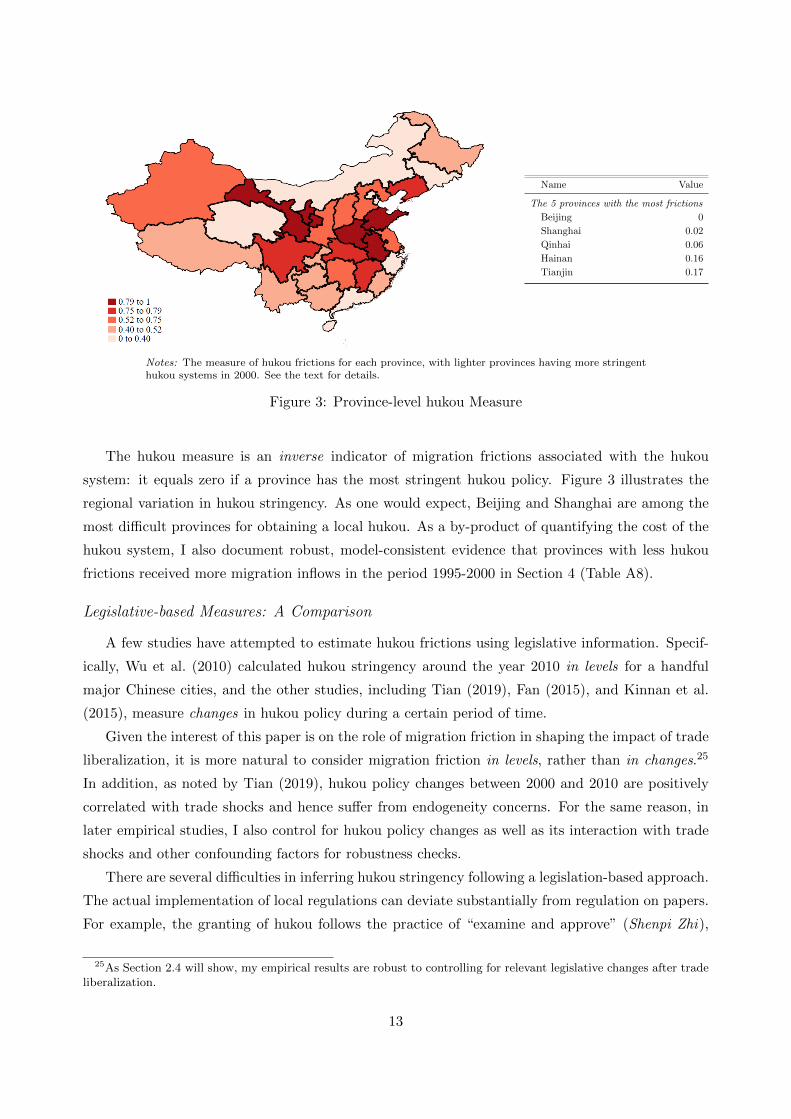
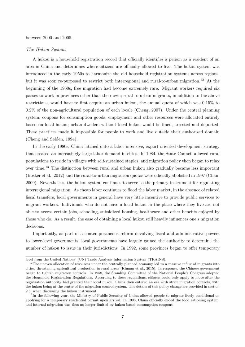
Name Value

The 5 provinces with the most frictions

Beijing 0

Shanghai 0.02

Qinhai 0.06

Hainan 0.16

Tianjin 0.17

Notes: The measure of hukou frictions for each province, with lighter provinces having more stringenthukou systems in 2000. See the text for details.

Figure 3: Province-level hukou Measure

The hukou measure is an inverse indicator of migration frictions associated with the hukou

system: it equals zero if a province has the most stringent hukou policy. Figure 3 illustrates the

regional variation in hukou stringency. As one would expect, Beijing and Shanghai are among the

most difficult provinces for obtaining a local hukou. As a by-product of quantifying the cost of the

hukou system, I also document robust, model-consistent evidence that provinces with less hukou

frictions received more migration inflows in the period 1995-2000 in Section 4 (Table A8).

Legislative-based Measures: A Comparison

A few studies have attempted to estimate hukou frictions using legislative information. Specif-

ically, Wu et al. (2010) calculated hukou stringency around the year 2010 in levels for a handful

major Chinese cities, and the other studies, including Tian (2019), Fan (2015), and Kinnan et al.

(2015), measure changes in hukou policy during a certain period of time.

Given the interest of this paper is on the role of migration friction in shaping the impact of trade

liberalization, it is more natural to consider migration friction in levels, rather than in changes.25

In addition, as noted by Tian (2019), hukou policy changes between 2000 and 2010 are positively

correlated with trade shocks and hence suffer from endogeneity concerns. For the same reason, in

later empirical studies, I also control for hukou policy changes as well as its interaction with trade

shocks and other confounding factors for robustness checks.

There are several difficulties in inferring hukou stringency following a legislation-based approach.

The actual implementation of local regulations can deviate substantially from regulation on papers.

For example, the granting of hukou follows the practice of “examine and approve” (Shenpi Zhi),

25As Section 2.4 will show, my empirical results are robust to controlling for relevant legislative changes after tradeliberalization.

13

satisfying application criteria does not guarantee migrants a local hukou.26 Historical data on

hukou-related laws and regulations are often limited, and hukou granting rules are not always de-

tailed (Kinnan et al., 2015). Moreover, even the same regulation can be very different in terms of

effectively monitoring migration in different regions (e.g., housing policy). The only exception is

Wu et al. (2010), who takes into account the degree of difficulties behind the regulatory content

across Chinese regions, but due to data limitation their analysis has been restricted in a subset

of prefectures. In addition, how to quantify different regulatory or regulatory adjustments is a

rather subjective decision, which could lead to inconsistency results across papers. The huku fric-

tion measure developed in this paper does not suffer from these concerns, hence serves as a good

complements to evaluate the hukou stringency across Chinese regions.

Finally, I provides a visual comparison of hukou measures constructed based on different ap-

proaches. Figure A8 plots the hukou measure developed in this paper against that of Fan (2015)

and Wu et al. (2010). I provide the comparison both at the province level, by aggregating their

measures with a simple average, and at the city level, by alternatively using the city-level measure

constructed based on my approach (which I also use for robustness checks in later sections). My

measure is strongly positively correlated with that of Wu et al. (2010) in both cases (Spearman

correlation 0.65, 0.54). The correlation with that of Fan (2015) is positive at the province level

but close to zero at the city level. This is perhaps not surprising, because both Wu et al. (2010)

and I address hukou friction in levels, while Fan (2015) considers hukou policy changes. For ex-

ample according to Fan (2015), Beijing is one of the regions that had the most frequent legislative

changes between 2000-2010, however it does not imply that Beijing has one of the most relaxed

hukou systems in China. Overall, the comparison suggests that my measure is broadly consistent

with the legislation-based measure when the latter is in levels and accounts for legislative details,

but legislation-based measures can be sensitive to their construction methods.

2.3 Empirical Results

Given the regional input tariff cuts and the hukou measure at hand, I examine the impact of input

liberalization on labor adjustments using the following specifications:

∆Yi = β1∆RITi +Dp + X1γ + εi, (1)

and

∆Yi = β2∆RITi + β3∆RITi ∗Hukoup +Dp + X′2γ + εi, (2)

26During the development of this project, I conducted detailed interviews with police officers in several Chineseregions. The general message is that there are many ‘hidden’ regulations and red tape, and frictions are also muchmore prevalent in less developed regions, such as Yunan, than in developed regions, such as Jiangsu.

14

where the second specification explores the heterogeneous regional effect of input tariff reductions

depending on the hukou frictions. Here, ∆Yi is the decadal change of the logged value of a regional

outcome variable such as employment or total population; β1 captures the regional effect of input

trade liberalization on the variable of interest during the 2000-2010 period, while β2 and β3 represent

the heterogeneous impacts of input tariff reductions depending on hukou frictions; the Dp terms

are province fixed effects, and X represents a set of additional controls. In the main specification,

I include regional output tariff and external tariff reductions to control for the effect of increased

import competition and improved market access after China’s WTO accession, respectively.27 In

addition, I include the pre-liberalization level of the outcome variable to allow for possible mean

convergence. Hukoup is the hukou friction measure; in the second specification, its interactions

with external and output tariff reductions are also included. The standard errors are clustered at

the provincial level (31 provinces), accounting for the possible covariance between the error terms

across prefectures within the same province.

Pattern 1: Prefectures facing larger input tariff cuts experience a relative increase in employment,

and the effect is stronger in provinces with less hukou frictions.

Table 2 presents the results of regressing employment changes on regional input tariff cuts. These

regressions are weighted by the log of beginning-of-period employment. Columns (1)-(3) present

the model without interactions. Column (1) shows the OLS results. Column (2) includes baseline

controls, and column (3) further includes province fixed effects to control for province-specific trends.

The estimate of 5.10 in column (3) implies that a 1-percentage-point regional input tariff cut was

associated with an approximately 5-percentage-point relative employment increase. The difference

between regional input tariff cuts in regions at the 95th and 5th percentiles is 3.27 percentage

points. Evaluated using the estimate in column (3), a prefecture at the 95th percentile experienced

a 16.68-percentage-point larger employment increase than a prefecture at the 5th percentile.

Columns (4)-(6) explore whether input-liberalization-induced employment adjustments were

more pronounced in provinces with less-stringent hukou systems. Similar to the case without inter-

actions, I first present the OLS results in column (4) and then add additional controls in columns

(5) and (6). As I normalized the hukou measure to a unit interval, coefficients on ∆RIT can be

interpreted as the impact of input tariff cuts in prefectures with the highest hukou frictions. In the

preferred specification in column (6), input tariff reductions had no impact on regional employment

in the prefectures with the most stringent hukou policies. In contrast, in regions with the most

relaxed hukou systems, a 1-percentage-point increase in input tariff cuts led to a 17-percentage-

point relative increase in employment,28 much larger than the 5-percentage-point average found in

column (3). This number may appear excessive, but note that the employment in the most-migrant-

27External tariff reductions capture the positive impact of tariff reductions by China’s trading partners after itsWTO accession; note that most countries had already granted China MFN status before 2001.

2818.45 − 1.18 ≈ 17. The sum of β2 and β3 is statistically significant unless otherwise stated.

15

Table 2: Effect of Input Tariff Cuts on Local Employment

Main With Hukou Interactions

(1) (2) (3) (4) (5) (6)

Regional input tariff cuts 6.76*** 6.92*** 5.10*** 1.35 3.19* -1.18

(1.72) (0.94) (1.65) (2.62) (1.67) (2.02)

Regional input tariff cuts × Hukou 10.88** 7.28** 18.45***

(4.72) (3.12) (6.05)

Regional output tariff change -2.69*** -2.48*** -2.51** -3.81***

(0.66) (0.72) (1.04) (1.31)

External tariff change 0.21 0.24 -0.23 0.04

(0.19) (0.22) (0.25) (0.30)

Initial employment -0.02 -0.00 -0.01 -0.01

(0.01) (0.01) (0.01) (0.01)

Regional output tariff change × Hukou 0.98 5.34*

(1.84) (3.10)

External tariff change × Hukou 0.82 0.37

(0.55) (0.47)

Province fixed effects Yes Yes

Observations 337 337 337 337 337 337

R-squared 0.32 0.46 0.66 0.43 0.51 0.69

Notes: The dependent variable is the 10-year change in logged prefecture employment. The sample contains 333 prefecturesand four directly controlled municipalities. Robust standard errors in parentheses are adjusted for 31 province clusters.Models are weighted by the log of beginning-of-period prefecture employment. *** p<0.01, ** p<0.05, * p<0.1.

receiving prefecture increased by over 60% over the 2000-2010 period. In all cases, the coefficient

on the interaction term is positive and statistically significant.

Consistent with the existing literature, regional output tariff reductions had a negative impact

on employment, although of a smaller magnitude than the impact of input tariff cuts. The effects of

external tariff reductions and their interaction with the hukou measure have the expected positive

sign but are statistically insignificant. The relaxed hukou system seems to have mitigated the

negative impact of output tariff reduction, but the results are less robust.29 Calculated based on

the specification in column (6), when taking into account both input and output channels, 29 percent

of the regional variation in employment changes can be accounted for by trade liberalization, most

of which is explained by the input tariff cuts.30

Pattern 2: The total population and the working age population react to input tariff cuts and their

interaction with the hukou measure in a quantitatively similar way to that of employment.

To validate that the spatial reallocation of labor drives pattern 1, I next examine how the

total and working age (15 to 64 years of age) populations responded to tariff changes. If the

observed employment changes were mainly due to intraregional adjustments, such as changes in

29Additionally, I find no statistically significant evidence that hukou frictions have shaped the effect of output tariffreduction on local population or migration inflows, as reported in Table 3.

30The partial R-squared of regional input tariff cuts, regional output tariff cuts and their interactions with the hukoumeasure is 0.29. The partial R-squared of regional input tariff cuts and their interaction with the hukou measure is0.21, while those of output tariff cuts and external tariff cuts are only 0.03 and 0.002, respectively.

16

the unemployment or labor participation rate, trade shocks should have had no impact on the

local population, whereas if the changes were primarily due to interregional adjustments, the local

population should react to trade shocks in a quantitatively similar manner to that of employment.

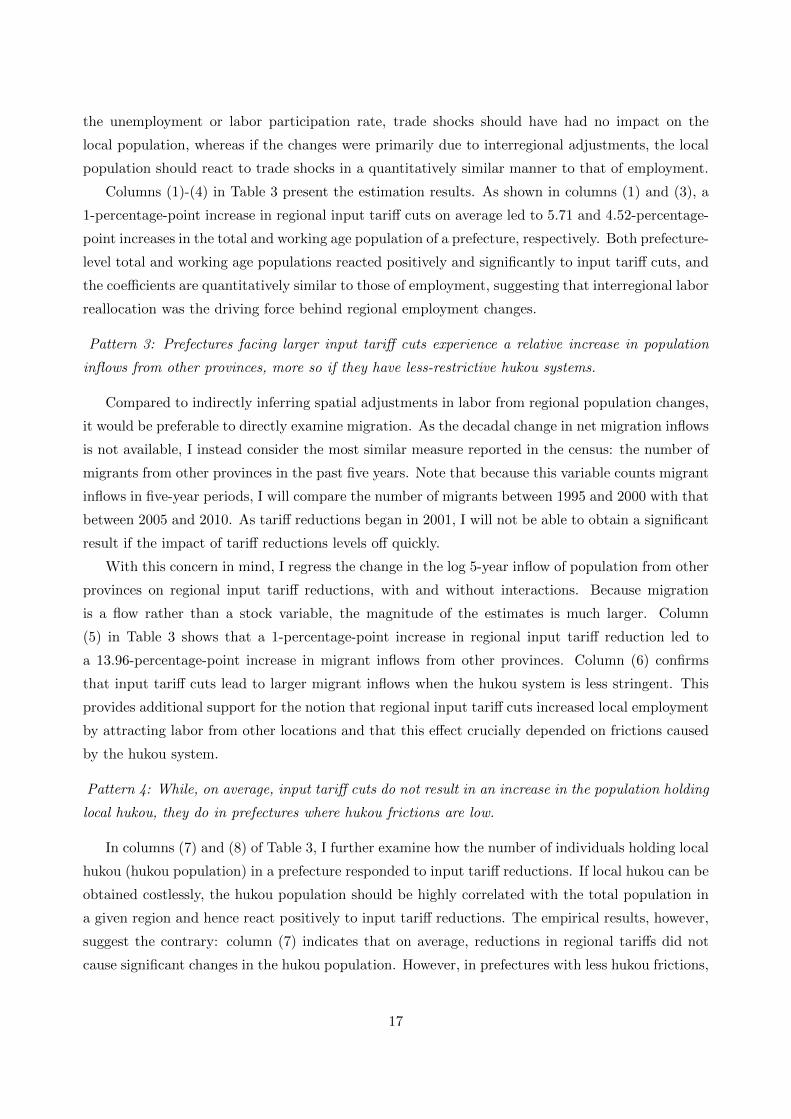
Columns (1)-(4) in Table 3 present the estimation results. As shown in columns (1) and (3), a

1-percentage-point increase in regional input tariff cuts on average led to 5.71 and 4.52-percentage-

point increases in the total and working age population of a prefecture, respectively. Both prefecture-

level total and working age populations reacted positively and significantly to input tariff cuts, and

the coefficients are quantitatively similar to those of employment, suggesting that interregional labor

reallocation was the driving force behind regional employment changes.

Pattern 3: Prefectures facing larger input tariff cuts experience a relative increase in population

inflows from other provinces, more so if they have less-restrictive hukou systems.

Compared to indirectly inferring spatial adjustments in labor from regional population changes,

it would be preferable to directly examine migration. As the decadal change in net migration inflows

is not available, I instead consider the most similar measure reported in the census: the number of

migrants from other provinces in the past five years. Note that because this variable counts migrant

inflows in five-year periods, I will compare the number of migrants between 1995 and 2000 with that

between 2005 and 2010. As tariff reductions began in 2001, I will not be able to obtain a significant

result if the impact of tariff reductions levels off quickly.

With this concern in mind, I regress the change in the log 5-year inflow of population from other

provinces on regional input tariff reductions, with and without interactions. Because migration

is a flow rather than a stock variable, the magnitude of the estimates is much larger. Column

(5) in Table 3 shows that a 1-percentage-point increase in regional input tariff reduction led to

a 13.96-percentage-point increase in migrant inflows from other provinces. Column (6) confirms

that input tariff cuts lead to larger migrant inflows when the hukou system is less stringent. This

provides additional support for the notion that regional input tariff cuts increased local employment

by attracting labor from other locations and that this effect crucially depended on frictions caused

by the hukou system.

Pattern 4: While, on average, input tariff cuts do not result in an increase in the population holding

local hukou, they do in prefectures where hukou frictions are low.

In columns (7) and (8) of Table 3, I further examine how the number of individuals holding local

hukou (hukou population) in a prefecture responded to input tariff reductions. If local hukou can be

obtained costlessly, the hukou population should be highly correlated with the total population in

a given region and hence react positively to input tariff reductions. The empirical results, however,

suggest the contrary: column (7) indicates that on average, reductions in regional tariffs did not

cause significant changes in the hukou population. However, in prefectures with less hukou frictions,

17

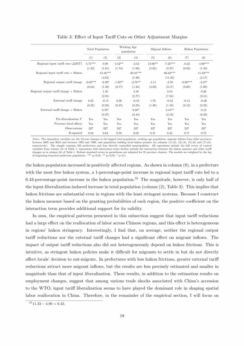
Table 3: Effect of Input Tariff Cuts on Other Adjustment Margins

Total PopulationWorking Age

Migrant Inflows Hukou Populationpopulation

(1) (2) (3) (4) (5) (6) (7) (8)

Regional input tariff cuts (∆RIT ) 5.71*** 0.98 4.52** -2.52 13.96** -7.25*** -0.23 -4.90***

(1.22) (1.61) (1.74) (1.98) (5.65) (2.37) (0.83) (1.56)

Regional input tariff cuts × Hukou 13.16*** 20.31*** 66.62*** 11.33***

(4.62) (5.46) (11.82) (3.17)

Regional output tariff change -2.63*** -2.39* -1.92** -2.78** -4.11 -2.76 -3.90*** -3.57*

(0.64) (1.39) (0.77) (1.24) (3.03) (3.17) (0.69) (1.99)

Regional output tariff change × Hukou 1.25 4.59 3.54 0.26

(2.91) (2.77) (7.34) (3.51)

External tariff change 0.25 -0.15 0.26 -0.16 1.70 -0.52 -0.14 -0.26

(0.25) (0.28) (0.25) (0.25) (1.38) (1.43) (0.12) (0.22)

External tariff change × Hukou 0.76* 0.80* 4.54** 0.12

(0.37) (0.44) (2.19) (0.29)

Pre-liberalization Y Yes Yes Yes Yes Yes Yes Yes Yes

Province fixed effects Yes Yes Yes Yes Yes Yes Yes Yes

Observations 337 337 337 337 337 337 337 337

R-squared 0.84 0.64 0.58 0.62 0.41 0.45 0.71 0.73

Notes: The dependent variables are the 10-year changes in the logged total population, working age population, migrant inflows from other provincesbetween 2005 and 2010 and between 1995 and 1990, and population holding local hukou permits (in columns (1)-(2), (3)-(4), (5)-(6) and (7)-(8),respectively). The sample contains 333 prefectures and four directly controlled municipalities. All regressions include the full vector of controlvariables from column (3) of Table 1; regressions with interaction terms further include the interaction between the hukou measure and other tariffchanges as in column (6) of Table 1. Robust standard errors in parentheses are adjusted for 31 province clusters. The models are weighted by the logof beginning-of-period prefecture population. *** p<0.01, ** p<0.05, * p<0.1.

the hukou population increased in positively affected regions. As shown in column (8), in a prefecture

with the most free hukou system, a 1-percentage-point increase in regional input tariff cuts led to a

6.43-percentage-point increase in the hukou population.31 The magnitude, however, is only half of

the input-liberalization-induced increase in total population (column (2), Table 3). This implies that

hukou frictions are substantial even in regions with the least stringent systems. Because I construct

the hukou measure based on the granting probabilities of each region, the positive coefficient on the

interaction term provides additional support for its validity.

In sum, the empirical patterns presented in this subsection suggest that input tariff reductions

had a large effect on the reallocation of labor across Chinese regions, and this effect is heterogeneous

in regions’ hukou stringency. Interestingly, I find that, on average, neither the regional output

tariff reductions nor the external tariff changes had a significant effect on migrant inflows. The

impact of output tariff reductions also did not heterogeneously depend on hukou frictions. This is

intuitive, as stringent hukou policies make it difficult for migrants to settle in but do not directly

affect locals’ decision to out-migrate. In prefectures with less hukou frictions, greater external tariff

reductions attract more migrant inflows, but the results are less precisely estimated and smaller in

magnitude than that of input liberalization. These results, in addition to the estimation results on

employment changes, suggest that among various trade shocks associated with China’s accession

to the WTO, input tariff liberalization seems to have played the dominant role in shaping spatial

labor reallocation in China. Therefore, in the remainder of the empirical section, I will focus on

3111.33 − 4.90 = 6.43.

18

the impact of input liberalization and its interaction with hukou frictions. I view the reduced-form

exercise as a transparent way to demonstrate the major economic force at play and to guide my

model construction. The task of quantifying the general equilibrium effects of tariff reductions and

the importance of hukou frictions is relegated to the quantitative section.

2.4 Confounding Factors to Trade Liberalization

In this and the following subsections, I present a battery of robustness checks of my baseline results.

For brevity, I focus on pattern 1; the results on other regional adjustments are available upon

request.

Contemporaneous Shocks

An important concern with my findings is that in addition to input liberalization, there might be

other concurrent policy or economic shocks that affect labor adjustments across regions. Specifically,

I examine how the pre-liberalization trends, SOE reforms, currency appreciation, housing booms,

agglomeration into regional capitals, and the development of Special Economic Zones could affect the

results. To control for pre-liberalization trends, I digitalize the 1990 population census tabulation

by provinces and compute the logged prefecture-level employment change between 1990 and 2000.

I employ the data from Annual Surveys of Industries (AIS) to construct the regional shifts in the

employment share of SOEs between 2000 and 2009 to account for the massive layoffs from the late

1990s that were due to SOE reforms.32 To control for the impact of currency appreciation, I compute

the changes in the regional exchange rate as follows: I first calculate the industry-prefecture-specific

change in logged real exchange rates between 2000 and 2010 as a trade-share-weighted average

across partner countries; I then average the variable across industries with δis being the weight. To

account for possible agglomeration into regional capitals, I control for capital fixed effects. Finally,

I exclude the 7 prefectures with Special Economic Zones.

In column (1) of Table 4, I report the result of regressing employment changes on regional input

tariff cuts, accounting for all of the above-mentioned factors. Including the full set of additional

controls leads to a lower coefficient on ∆RIT , but it remains positively significant. Column (2)

reports the results with interaction terms: the estimate of the interaction between ∆RIT and the

hukou friction is in line with the baseline case and is statistically significant at the 5% level. Tables

A4 and A5 additionally report the regression results when controlling for one factor at a time

without and with interaction terms, respectively.

Exogeneity of Trade Liberalization

To draw any causal implications of input trade liberalization, the observed tariff changes must

32I choose not to use the data of the year 2010, as they contain erroneous information on employment statistics.Brandt et al. (2014) provide an excellent summary of the data issues of the AIS database.

19

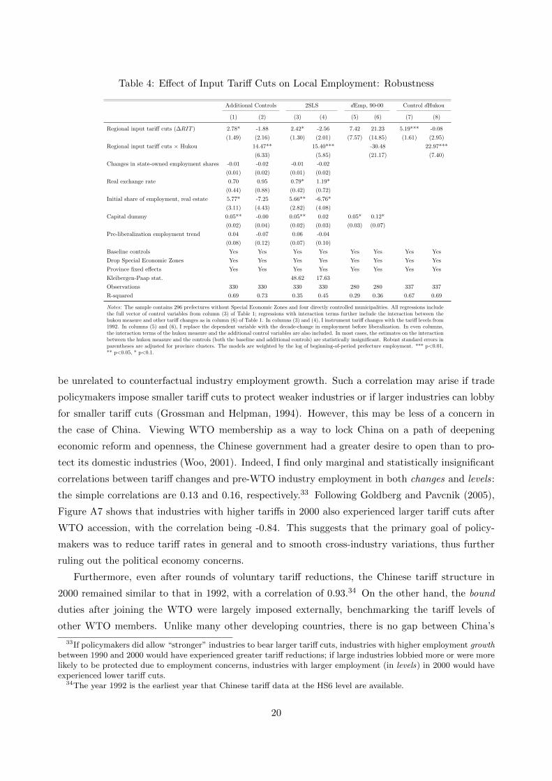
Table 4: Effect of Input Tariff Cuts on Local Employment: Robustness

Additional Controls 2SLS dEmp, 90-00 Control dHukou

(1) (2) (3) (4) (5) (6) (7) (8)

Regional input tariff cuts (∆RIT ) 2.78* -1.88 2.42* -2.56 7.42 21.23 5.19*** -0.08

(1.49) (2.16) (1.30) (2.01) (7.57) (14.85) (1.61) (2.95)

Regional input tariff cuts × Hukou 14.47** 15.40*** -30.48 22.97***

(6.33) (5.85) (21.17) (7.40)

Changes in state-owned employment shares -0.01 -0.02 -0.01 -0.02

(0.01) (0.02) (0.01) (0.02)

Real exchange rate 0.70 0.95 0.79* 1.19*

(0.44) (0.88) (0.42) (0.72)

Initial share of employment, real estate 5.77* -7.25 5.66** -6.76*

(3.11) (4.43) (2.82) (4.08)

Capital dummy 0.05** -0.00 0.05** 0.02 0.05* 0.12*

(0.02) (0.04) (0.02) (0.03) (0.03) (0.07)

Pre-liberalization employment trend 0.04 -0.07 0.06 -0.04

(0.08) (0.12) (0.07) (0.10)

Baseline controls Yes Yes Yes Yes Yes Yes Yes Yes

Drop Special Economic Zones Yes Yes Yes Yes Yes Yes Yes Yes

Province fixed effects Yes Yes Yes Yes Yes Yes Yes Yes

Kleibergen-Paap stat. 48.62 17.63

Observations 330 330 330 330 280 280 337 337

R-squared 0.69 0.73 0.35 0.45 0.29 0.36 0.67 0.69

Notes: The sample contains 296 prefectures without Special Economic Zones and four directly controlled municipalities. All regressions includethe full vector of control variables from column (3) of Table 1; regressions with interaction terms further include the interaction between thehukou measure and other tariff changes as in column (6) of Table 1. In columns (3) and (4), I instrument tariff changes with the tariff levels from1992. In columns (5) and (6), I replace the dependent variable with the decade-change in employment before liberalization. In even columns,the interaction terms of the hukou measure and the additional control variables are also included. In most cases, the estimates on the interactionbetween the hukou measure and the controls (both the baseline and additional controls) are statistically insignificant. Robust standard errors inparentheses are adjusted for province clusters. The models are weighted by the log of beginning-of-period prefecture employment. *** p<0.01,** p<0.05, * p<0.1.

be unrelated to counterfactual industry employment growth. Such a correlation may arise if trade

policymakers impose smaller tariff cuts to protect weaker industries or if larger industries can lobby

for smaller tariff cuts (Grossman and Helpman, 1994). However, this may be less of a concern in

the case of China. Viewing WTO membership as a way to lock China on a path of deepening

economic reform and openness, the Chinese government had a greater desire to open than to pro-

tect its domestic industries (Woo, 2001). Indeed, I find only marginal and statistically insignificant

correlations between tariff changes and pre-WTO industry employment in both changes and levels:

the simple correlations are 0.13 and 0.16, respectively.33 Following Goldberg and Pavcnik (2005),

Figure A7 shows that industries with higher tariffs in 2000 also experienced larger tariff cuts after

WTO accession, with the correlation being -0.84. This suggests that the primary goal of policy-

makers was to reduce tariff rates in general and to smooth cross-industry variations, thus further

ruling out the political economy concerns.

Furthermore, even after rounds of voluntary tariff reductions, the Chinese tariff structure in

2000 remained similar to that in 1992, with a correlation of 0.93.34 On the other hand, the bound

duties after joining the WTO were largely imposed externally, benchmarking the tariff levels of

other WTO members. Unlike many other developing countries, there is no gap between China’s

33If policymakers did allow “stronger” industries to bear larger tariff cuts, industries with higher employment growthbetween 1990 and 2000 would have experienced greater tariff reductions; if large industries lobbied more or were morelikely to be protected due to employment concerns, industries with larger employment (in levels) in 2000 would haveexperienced lower tariff cuts.

34The year 1992 is the earliest year that Chinese tariff data at the HS6 level are available.

20

bound and applied duties, and the binding coverage is 100%. If the pre-liberalization tariffs were

highly correlated with the protection structure set a decade earlier while the post-liberalization

tariffs were externally set, it is unlikely that tariff reductions between 2000 and 2005 in China

would be correlated with counterfactual industry employment changes. To further address this

concern, I instrument tariff changes with year-1992 tariff levels,35 in addition to controlling for

other confounding factors. Columns (3) and (4) of Table 4 report the two-stage results: a 1-

percentage-point regional input tariff cut led to a 2.42-percentage-point employment increase on

average and a 15.40-percentage-point employment increase in regions with the most relaxed hukou

systems. The magnitudes are quantitatively very similar to those of the OLS estimation results in

columns (1) and (2).

Pre-liberalization Employment Changes

Finally, to verify that my results are not due to spurious correlation, I regress pre-liberalization

employment changes (1990-2000) on regional input tariff cuts, using the employment share from 1990

to compute ∆RIT .36 The results are presented in columns (5) and (6) of Table 4. Regional input

tariff cuts had no statistically significant impact on pre-liberalization employment; the interaction

term is also statistically insignificant and has the opposite sign.37

Trade-induced Institutional Changes

Another important concern with my findings is that hukou policies themselves might also change

in response to trade liberalization. If increased labor demand results in local governments relaxing

migration policies in prefectures positively affected by trade shocks, my estimates of the interaction

between hukou friction and ∆RIT may be biased upwards. To address this concern, I further control

for the hukou-related legislative change index developed by Fan et al. (2015). The estimation results

are reported in columns (7) and (8) of Table 4: a 1-percentage-point reduction in the regional input

tariff led to a 5.19-percentage-point employment increase on average and a 22.97-percentage-point

employment increase in regions with the most relaxed hukou systems, very similar to the baseline

results.

2.5 Validity of the Hukou Measure

Alternative Measures

35Specifically, I construct an instrument following the formula of ∆RIT but replace the 2000-2005 tariff changeswith the 1992 tariff levels. Similarly, I also instrument regional output tariff changes using the 1992 tariff levels.

36The industry classification was more aggregated in 1990; hence, I calculate regional tariff cuts based on 61industries. The 1990 regional employment by sector is missing for some prefectures. To ensure data quality, I workwith 287 prefecture-level cities that have employment information for all industries.

37These results are not driven by different levels of industrial aggregation or decreased sample size: when I use thesame sample of prefectures, regressing 2000-2010 employment changes on ∆RIT , which is calculated based on the61 industries, I obtain positive and significant estimates, and they are quantitatively in line with the baseline results(available upon request).

21

Table 5: Changes in Migration Inflow by Individual Types

Skill TypeWorking Migrants

Placebo: Marriage Migrants

High-skilled Low-skilled Levels Shares

(1) (2) (3) (4) (5) (6) (7) (8) (9) (10)

Regional input tariff cuts (∆RIT ) 32.26*** -6.71 20.53*** -1.93 27.25*** -6.42 7.69* 5.29 -39.97*** 1.41

(8.11) (9.13) (5.72) (7.39) (6.88) (9.78) (4.38) (15.65) (10.72) (16.44)

Regional input tariff cuts × Hukou 97.80*** 73.82*** 108.67*** 7.28 -113.41***

(22.83) (20.83) (21.63) (35.06) (35.19)

Baseline Controls Yes Yes Yes Yes Yes Yes Yes Yes Yes Yes

Province FEs Yes Yes Yes Yes Yes Yes Yes Yes Yes Yes

Observations 184 184 328 328 304 304 243 243 243 243

R-squared 0.40 0.44 0.46 0.47 0.39 0.41 0.51 0.52 0.37 0.41

Notes: Columns (1)-(8) present the impact of input tariff cuts on labor inflows by 4 individual (age 15-65, not in school) types: high-skilled workers,low-skilled workers, migrants who moved for working purpose, and migrants who moved for marriage reasons, respectively. Columns (9)-(10) present theimpact of input tariff cuts on the share of marriage migrants in total migrants. All regressions include the full vector of control variables from column (3)of Table 1; models with interaction terms further include the interaction between the hukou measure and other tariff changes as in column (6) of Table 1.All dependent variables are calculated using the 0.095% sample of the 2000 population census and 0.1% sample of the 2010 population census. Althoughthe National Assembly reported positive labor inflows in all prefectures, I observe prefectures with zero inflows due to my limited micro-sample size. Thoseprefectures are dropped from the analysis. Robust standard errors are in parentheses. The models are weighted by the log of beginning-of-period prefecturepopulation. *** p<0.01, ** p<0.05, * p<0.1.

Table A6, columns (1)-(8), presents a set of robustness checks using alternative hukou friction

measures. In column (1), I run the regression with the simple hukou-granting probabilities (without

adjusting for individual characteristics) as the hukou measure. In column (2), I instead use a measure

constructed based on province fixed effects. Specifically, I regress the hukou-granting dummy on

individual characteristics and province fixed effects (instead of prefecture fixed effects) and then

normalize the estimates on the fixed effects as my measure of hukou frictions. In column (3), I

directly use the prefecture fixed effects as the hukou friction measure. In all cases, the coefficients

on the interaction terms remain positive and significant and are quantitatively similar to the baseline

results, suggesting that my baseline findings are unlikely to be driven by the specific way I aggregate

the hukou friction measure.

It is possible that the fixed effects are not precisely estimated for prefectures with low migration

inflows. To address this concern, in column (4), I construct the provincial hukou friction measure as

the inverse-standard-error-weighted average of prefecture fixed effects instead of the simple average.

The idea is to assign lower weights to prefecture hukou frictions that are not precisely estimated. In

column (5), I drop prefectures with fewer than 30 migrants when constructing the hukou measure.

The estimation results are robust when using these alternative hukou measures.

The Composition of Migration Inflows

Another concern is that my estimation results may be biased if prefectures receive different mixes

of migrants. For instance, high-skilled workers tend to be more mobile than low-skilled workers. If

regions with low hukou frictions happened to attract more skilled workers after trade liberalization,

total migration might appear to respond more to trade shocks in these regions. Another example

is that individuals who migrate to marry a local will have easier access to local hukou, and my

baseline results might simply capture its spurious correlation with the hukou frictions. To address

22

these concerns, I use the microdata sample of censuses in 2000 and 2010 to construct prefecture-level

migrant inflows by skill groups and for migration reasons.

Table 5 reports the impact of input liberalization on different types of migration inflows: high-

skilled workers, low-skilled workers, migrants who moved for working reasons, and migrants who

moved for marriage purposes. I focus on working-age individuals and exclude those who moved for

education or were in school when they were surveyed. As shown in columns (1)-(4), both high-skilled

and low-skilled workers responded positively to input liberalization, and the effect was stronger in

regions with low hukou frictions. Consistent with my conjecture, high-skilled workers tended to be

more mobile and hence more responsive to trade shocks and sensitive to hukou policies. However,

the magnitudes of the estimated coefficients are comparable to those of the low-skilled coefficients

and are not significantly different from one another. This is also true for the working migrants, as

shown in columns (5)-(6). In short, my results are robust to considering migrants of different skill

types and to focusing solely on individuals who moved for working reasons.

In columns (7)-(10), I use migrants who moved for marriage purposes as a placebo. If the

change in marriage migration is what drives my baseline results, one should expect that the share

of marriage migrants increased more in regions with higher input tariff changes, and such an increase

would have to be more pronounced in areas with low hukou frictions. However, columns (9)-(10)

show the opposite results, suggesting that this conjecture is unlikely to be true. In fact, the share of

marriage migrants dropped in regions with higher ∆RIT . The reason is that although the number

of migrants who moved for marriage purposes increased slightly in regions with higher input tariff

cuts, it did so considerably less than that for working migrants (see the estimation results in levels

in columns (5) and (7)). This also suggests that where people move for marriage purposes might

depend on various factors other than economic ones. The insignificant interaction term in column

(8) confirms that migration for marriage purposes is less affected by the hukou system.

Unobserved Heterogeneity

Although I have demonstrated that my results are robust to examining migrants by skill type

and focusing on working migrants only, one could still be concerned about the role of unobserved

heterogeneity. For instance, migrant workers who choose to work in stricter regions may have better

information about the area or face better job offers due to selection. However, these unobserved

heterogeneities are likely to be positively correlated with migrants’ probability of obtaining hukou

and therefore impose downward bias on the regression results. To further address this concern, I

replace the hukou measure with a dummy variable equaling 1 if the friction is below the median.

The dummy measure is more robust to measurement errors than a continuous variable. The results

remain robust as shown in column (8) of Table A6: in regions with an above-median relaxed Hukou

system, a 1-percentage-point increase in input tariff cuts led to 6-percentage-point relative increase

in employment compared to regions below the median.

23

The Demand for Local Hukou

The validity of my hukou measure crucially depends on the assumption that it captures the

stringency of hukou supply instead of demand-side factors. Because I do not observe migrants’

hukou application decisions, a low hukou-obtaining probability in a region may simply reflect a lack

of demand. For instance, if there are very few gains from accessing a location’s hukou, or if migrants

expect to migrate temporarily, they may not request a local hukou.

The above-mentioned conjectures are theoretically possible but are unlikely to be the case in

reality for multiple reasons. First, as various social benefits are tied to the local hukou, it is difficult

to imagine that migrants would not request one if they could obtain it without any cost.38 Moreover,

for public services that hukou holders are eligible to access, such as education or health care, there

were very few private sector substitutes available in the 1990s, making the demand for a local hukou

almost inelastic. The lion’s share of temporary migrants came from rural areas: calculated using

the 2000 census data, 83% of the migrants who moved between 1995 and 2000 held a rural residence

permit.39 As urban hukou was much more attractive than rural hukou at the time, temporary

migrants were “temporary” precisely because of the difficulty in obtaining an urban hukou, not

because they did not want to settle permanently in the cities.40 Finally, a region may adopt a

strict hukou policy for various reasons (as discussed in Section 2.2); therefore, although there are

regional variations in hukou demand, as long as it does not positively correlate with hukou supply,

the baseline findings should be downward biased.

In addition, I provide two exercises to support my conjecture. I first show that my results are

robust to alternative hukou measures constructed using subsamples of migrants who were more likely

to demand local hukou regardless of their idiosyncratic preferences. Then, I use a unique group of

migrants who temporarily faced no hukou frictions, university students, to perform placebo tests.

Hukou measures based on subgroups If migrants did not want to obtain a local hukou

in some prefectures, the small value of my hukou measure might reflect their reluctance to apply

for local hukou rather than their limited supply. This issue is partly addressed by including the

GDP per capita difference between migrants’ destination and source provinces when constructing

the hukou measure, as people who moved to more developed regions should be more willing to

obtain a local hukou. In columns (6) and (7) of Table A6, I provide additional robustness checks by

constructing alternative hukou measures using subsamples of my data. In column (6), I focus solely

on migrants with local family ties, namely migrants who live with family members who already

38The importance of having a local hukou has been emphasized by many researchers. See Cheng and Selden (1994),Chan and Buckingham (2008), Montgomery (2012) and Chan (2009).

39The number is calculated based on migrants who had not obtained a local hukou in 2000 using the censusmicrodata. The share could be upward-biased if urban migrants were more likely to obtain a local hukou.

40I strictly refer to urban hukou when discussing the supply of and demand for hukou; since collectivization in the1950s, rural hukou has entailed membership in the village collective and was not given to migrants (Sun and Fan,2011). Almost all migration inflows in the periods I examine were towards cities. The divide between urban and ruralhukou creates an interesting environment for several areas of study, such as land tenure arrangements, which are notthe focus of this paper.

24

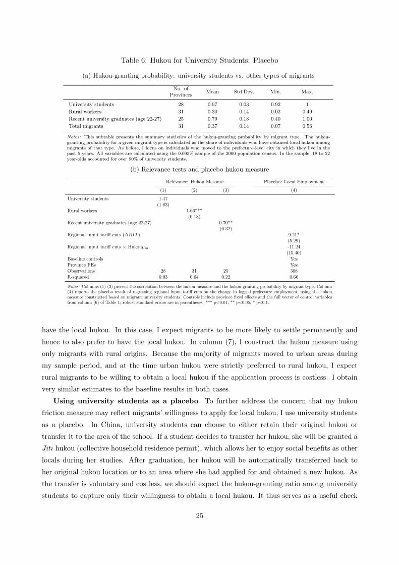
Table 6: Hukou for University Students: Placebo

(a) Hukou-granting probability: university students vs. other types of migrants

No. ofProvinces

Mean Std.Dev. Min. Max.

University students 28 0.97 0.03 0.92 1

Rural workers 31 0.30 0.14 0.02 0.49

Recent university graduates (age 22-27) 25 0.79 0.18 0.40 1.00

Total migrants 31 0.37 0.14 0.07 0.56

Notes: This subtable presents the summary statistics of the hukou-granting probability by migrant type. The hukou-granting probability for a given migrant type is calculated as the share of individuals who have obtained local hukou amongmigrants of that type. As before, I focus on individuals who moved to the prefecture-level city in which they live in thepast 5 years. All variables are calculated using the 0.095% sample of the 2000 population census. In the sample, 18 to 22year-olds accounted for over 90% of university students.

(b) Relevance tests and placebo hukou measure

Relevance: Hukou Measure Placebo: Local Employment

(1) (2) (3) (4)

University students 1.47(1.83)

Rural workers 1.66***(0.18)

Recent university graduates (age 22-27) 0.70**(0.32)

Regional input tariff cuts (∆RIT ) 9.21*(5.29)

Regional input tariff cuts × HukouUni -11.24(15.40)

Baseline controls YesProvince FEs YesObservations 28 31 25 308R-squared 0.03 0.64 0.22 0.66

Notes: Columns (1)-(3) present the correlation between the hukou measure and the hukou-granting probability by migrant type. Column(4) reports the placebo result of regressing regional input tariff cuts on the change in logged prefecture employment, using the hukoumeasure constructed based on migrant university students. Controls include province fixed effects and the full vector of control variablesfrom column (6) of Table 1; robust standard errors are in parentheses. *** p<0.01, ** p<0.05, * p<0.1.

have the local hukou. In this case, I expect migrants to be more likely to settle permanently and

hence to also prefer to have the local hukou. In column (7), I construct the hukou measure using

only migrants with rural origins. Because the majority of migrants moved to urban areas during

my sample period, and at the time urban hukou were strictly preferred to rural hukou, I expect

rural migrants to be willing to obtain a local hukou if the application process is costless. I obtain

very similar estimates to the baseline results in both cases.

Using university students as a placebo To further address the concern that my hukou

friction measure may reflect migrants’ willingness to apply for local hukou, I use university students

as a placebo. In China, university students can choose to either retain their original hukou or

transfer it to the area of the school. If a student decides to transfer her hukou, she will be granted a

Jiti hukou (collective household residence permit), which allows her to enjoy social benefits as other

locals during her studies. After graduation, her hukou will be automatically transferred back to

her original hukou location or to an area where she had applied for and obtained a new hukou. As

the transfer is voluntary and costless, we should expect the hukou-granting ratio among university

students to capture only their willingness to obtain a local hukou. It thus serves as a useful check

25

of whether my hukou measure captures the regional variations in hukou demand.

I first examine the simple hukou-granting probability for university students migrating for their

studies. Table 6 (a) presents the summary statistics. On average, 97% of university students chose to

obtain a new hukou, and the number varies little across provinces. This provides additional evidence

that the demand for local hukou is nearly inelastic. In contrast, for rural working migrants or for the

full population, the average granting probabilities were much lower (0.30 and 0.37), and the regional

variations were substantial. To address the concern that university students may have different skill

levels (which may affect hukou supply) and location preferences (which may affect hukou demand),

I also compare the student migrants to migrants who recently graduated from university. The

difference is still striking: for recent university graduates, the average hukou-granting probability is

nearly 20% lower, and the standard deviation is approximately 4 times larger.

Then, I use the sample of university student migrants to construct a hukou placebo. As shown

in column (1) of Table 6 (b), it explains little of the variation in the baseline friction measure (R-

squared of 0.03). In contrast, hukou frictions constructed based on rural migrants and university

graduates are both significantly correlated with the baseline measure, as shown in columns (2)-(3).

In column (4), I find no evidence that the placebo hukou measure shapes the impact of regional

input tariff cuts. In conclusion, although I cannot entirely rule out the possibility that the hukou

demand may contaminate my baseline results, the evidence presented in this subsection suggests

that it is less of a concern.

3 A Spatial Model with Migration Frictions

The previous section documents a significant impact of trade liberalization on spatial labor real-

location and that the impact is more pronounced in regions where hukou frictions are low. While

interesting in its own right, the reduced-form evidence abstracts from various general equilibrium

effects of trade reforms. In this section, I propose a quantitative spatial model to further explore the

general equilibrium effects of trade liberalization and to quantify the importance of hukou frictions.

I make one important deviation from existing spatial models of the Chinese economy, such as Fan

(2015) and Tombe and Zhu (2019), by allowing for a more realistic elasticity of factor substitution.

The key is to recognize that the Cobb-Douglas production function used in these and many other

spatial quantitative works is special. As noted by (Baqaee and Farhi, 2019b), under Cobb-Douglas,

Hulten’s theorem is globally accurate. This means that these models, by design, would imply that

the micro structure of an economy, including the extent of factor reallocation, will play no role in

affecting the gains from trade. This could also explain the close-to-zero interaction effect between

domestic geography and trade in Fan (2015), between commuting costs and trade liberalization in

Monte et al. (2015), and between factor misallocation and trade shocks in Ouyang (2021), among

26

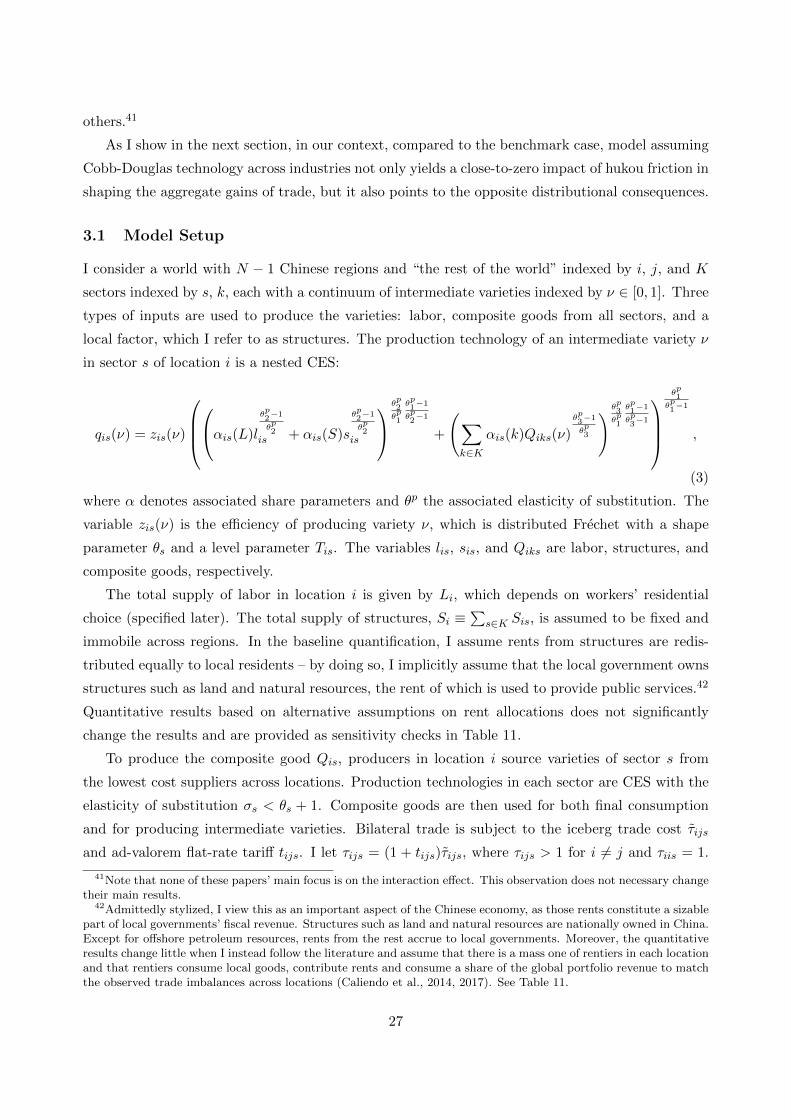
others.41

As I show in the next section, in our context, compared to the benchmark case, model assuming

Cobb-Douglas technology across industries not only yields a close-to-zero impact of hukou friction in

shaping the aggregate gains of trade, but it also points to the opposite distributional consequences.

3.1 Model Setup

I consider a world with N − 1 Chinese regions and “the rest of the world” indexed by i, j, and K

sectors indexed by s, k, each with a continuum of intermediate varieties indexed by ν ∈ [0, 1]. Three

types of inputs are used to produce the varieties: labor, composite goods from all sectors, and a

local factor, which I refer to as structures. The production technology of an intermediate variety ν

in sector s of location i is a nested CES:

qis(ν) = zis(ν)

αis(L)l

θp2−1

θp2

is + αis(S)s

θp2−1

θp2

is

θp2θp1

θp1−1

θp2−1

+

(∑k∈K

αis(k)Qiks(ν)

θp3−1

θp3

) θp3θp1

θp1−1

θp3−1

θp1

θp1−1

,

(3)

where α denotes associated share parameters and θp the associated elasticity of substitution. The

variable zis(ν) is the efficiency of producing variety ν, which is distributed Frechet with a shape

parameter θs and a level parameter Tis. The variables lis, sis, and Qiks are labor, structures, and

composite goods, respectively.

The total supply of labor in location i is given by Li, which depends on workers’ residential

choice (specified later). The total supply of structures, Si ≡∑

s∈K Sis, is assumed to be fixed and

immobile across regions. In the baseline quantification, I assume rents from structures are redis-

tributed equally to local residents – by doing so, I implicitly assume that the local government owns

structures such as land and natural resources, the rent of which is used to provide public services.42

Quantitative results based on alternative assumptions on rent allocations does not significantly

change the results and are provided as sensitivity checks in Table 11.

To produce the composite good Qis, producers in location i source varieties of sector s from

the lowest cost suppliers across locations. Production technologies in each sector are CES with the

elasticity of substitution σs < θs + 1. Composite goods are then used for both final consumption

and for producing intermediate varieties. Bilateral trade is subject to the iceberg trade cost τijs

and ad-valorem flat-rate tariff tijs. I let τijs = (1 + tijs)τijs, where τijs > 1 for i 6= j and τiis = 1.

41Note that none of these papers’ main focus is on the interaction effect. This observation does not necessary changetheir main results.

42Admittedly stylized, I view this as an important aspect of the Chinese economy, as those rents constitute a sizablepart of local governments’ fiscal revenue. Structures such as land and natural resources are nationally owned in China.Except for offshore petroleum resources, rents from the rest accrue to local governments. Moreover, the quantitativeresults change little when I instead follow the literature and assume that there is a mass one of rentiers in each locationand that rentiers consume local goods, contribute rents and consume a share of the global portfolio revenue to matchthe observed trade imbalances across locations (Caliendo et al., 2014, 2017). See Table 11.

27

Thus, τijs units of a variety in sector s must be shipped from location i for one unit to arrive at

location j. In the interest of brevity, I ignore tariff revenues for the present and account for them

when performing quantitative exercises.

Consumer preferences over composite goods from different industries are CES with share pa-

rameter βs and elasticity of substitution θ0 . The utility of worker ω holding a hukou from location

h and residing in location i depends on her goods consumption, idiosyncratic amenity shocks ai(ω),

and migration frictions dhi:

Uhi(ω) =ai(ω)yi(ω)

dhiPi, (4)

where the nominal income yi(ω) and the local consumption price index Pi jointly determine the

consumption level of worker ω. The idiosyncratic amenity shock ai(ω) captures the idea that workers

have heterogeneous preferences for living in different locations and are assumed to be drawn from

a Frechet distribution with a shape parameter κ > 1 and a level parameter Ai.

Living outside one’s hukou area is costly. For a worker holding hukou from region h, dhiPi units

of her income have to be spent for one unit of consumption in region i.43 I assume that dhi consists

of both the hukou frictions (Hhi) and other types of resettlement costs dhi such that dhi = Hhidhi,

where dhi > 1 for h 6= i and dhh = 1. In reality, the hukou system does not discriminate against

one’s origin among non-locals; therefore, Hhi = Hi > 1 for h 6= i and Hhh = 1.

Each worker chooses the location that offers her the highest utility and supplies one unit of labor

inelastically under perfect competition. The number of workers holding the hukou of a particular

location h is assumed to be fixed and is denoted as Lh. Labor is internationally immobile.

3.2 Equilibrium

Given the heterogeneous location preferences and the existence of migration frictions, wages can

differ across locations. However, with perfectly competitive labor markets wi(ω) must equalize

across workers in a given region. The unit input cost to produce a variety in sector s in location i

43In reality, the costs of hukou have three main aspects. First, not having a local hukou can entail additionalcosts of living due to institutional frictions: for instance, one can only take the university entrance examination, bemarried, or apply for a birth permit or visa application in one’s hukou city. Second, workers without a local hukoumay have lower bargaining power in the labor market and hence earn lower wages. Finally, one may face a higher barto access certain products, such as healthcare or education. In the last case, one may pay a higher price to access thosegoods (if possible), find private alternatives, or return to one’s hukou city to consume those goods. In any case, theyraise the cost of living for non-hukou holders but require additional (and different) assumptions on how those goodsare provided. Having no direct counterpart in the empirical analysis or guidance from real data, iceberg migrationcosts, given their brevity and straightforward interpretation, seem a reasonable case to consider first. Alternatively,I introduce a public sector following Caliendo et al. (2017) and Fajgelbaum et al. (2015) and assume that migrantworkers pay a higher price to access local public goods as a robustness check; the associated results are presented inTable 11.

28

is therefore:

cis =

(αis(L)θp2w

1−θp2i + αis(S)θ

p2r

1−θp2i

) 1−θp11−θp2 +

(∑k∈K

αis(k)θp3P

1−θp3ik

) 1−θp11−θp3

1

1−θp1

, (5)

where wi is the wage, ri is the rental rates of structures, and Pik is the price of the composite goods

in sector k in location i. From EK, location i’s share of expenditure on varieties from sector s,

location j is given by:

λjis =Tjs (τjiscjs)

−θs∑n∈N Tns (τniscns)

−θs . (6)

The price of the composite good in sector s, location i therefore is:

Pis = ηs

∑j∈N

Tjs(τjiscjs)−θs

− 1θs

, (7)

where ηs ≡ Γ( θs−σs+1θs

)1

1−σs and Γ(.) is a Gamma function. The corresponding local price index

is Pi = (∑

s∈K βsθ0P 1−θ0

is )1

1−θ0 . Total revenue in each location equals total expenditure on goods

produced in that location for both consumption and intermediate usage. Thus:

Ris =∑j∈N

λijs

(βjsYj +

∑k∈K

αjk(s)Rjk

), (8)

where Yj is the total value added of location j, βjs and αjk(s) are the equilibrium expenditure

shares of s in final consumption and in the production of goods k in location j, respectively.44 Each

worker’s income equals her wage plus the transferred rents from structures:

Yi = yiLi = wiLi + riSi. (9)

Equalizing the total wage payment to the total revenue that goes to workers yields the local labor

demand:

LDi =∑s∈K

αis(L)Ris/wi, (10)

where αis(L) is the equilibrium expenditure share of labor.45

Given the distribution of amenities, the probability that a worker with hukou h chooses to live

44Specifically, βjs =βθ0s P

1−θ0js∑

k∈K βkθ0P

1−θ0jk

and αjk(s) = αjk(s)θp3P

1−θp3js

(∑s∈K αjk(s)

θp3 P

1−θp3js

) 1−θp11−θp3

−1

c1−θp1jk

.

45Specifically, αis(L) =αis(L)

θp2w

1−θp2i c

θp1−1

is(αis(L)

θp2w

1−θp2i +αis(S)

θp2 r

1−θp2i

)1−1−θp11−θp2

and αis(S) =αis(S)

θp2 r

1−θp2i c

θp1−1

is(αis(L)

θp2w

1−θp2i +αis(S)

θp2 r

1−θp2i

)1−1−θp11−θp2

.

29

in location i is:

πhi =Ai

(yi

Pidhi

)κ∑

j∈N Aj

(yj

Pjdhj

)κ . (11)

Labor market clearing therefore implies:

∑s∈K

αis(L)Ris/wi =∑h∈N

πhiLh. (12)

Finally, the structure market clearing implies that the equilibrium rental rates can be determined

by equating the demand for and supply of structures:

∑s∈K

αis(S)Ris = Siri. (13)

Definition 1. Given Lh, Sis, τijs and dhi, an equilibrium is a wage vector {wi}i∈N , rental prices

{ri}i∈N , residential choices {πhi}h∈N,i∈N , and goods prices {Pis}i∈N,s∈K that satisfy equilibrium

conditions (5), (6), (7), (8), (9), (11), (12) and (13) for all i, h, s.

Intuitively, given wage wi and structure rents ri, one can solve for the equilibrium price Pis and

export shares λijs using equations (5), (6) and (7). Labor demand LDi and sector output Ris can

then be solved for using equations (8), (9) and (10). Higher factor prices imply a higher factor

supply but a lower factor demand. These two forces work against one another and pin down the

equilibrium values of wi and ri.

Compared to the standard spatial model where production technology and preferences at the

industry level are assumed to be Cobb-Douglas, it is evident that once we deviate from Cobb-

Douglas, the production and consumption share parameters, α and β, are no longer constant.

With trade cost reduction, their changes will depend on the rich substitution between goods and

production factors. Then, the whole production structure, and hence the factor demand, responds

endogenously to shocks, and the resulting nonlinearities are shaped by microeconomic details of the

economy.

3.3 Equilibrium in Relative Changes

How would the equilibrium change when tariffs or migration frictions change? I proceed as in Dekle

et al. (2008) and solve the equilibrium in relative changes. Using the x ≡ x′/x notation, where x′

is the value of x in the new equilibrium and x is the initial value, the equilibrium equation system

(5)-(9), (11), (12)-(13) can be rewritten as follows:

cis =

α1

(αis(L)

α1w

1−θp2i +

αis(S)

α1r

1−θp2i

) 1−θp11−θp2 + (1− α1)

(∑k∈K

αis(k)

1− α1P

1−θp3ik

) 1−θp11−θp3

1

1−θp1

; (14)

30

λjis =

(τjiscjs

Pis

)−θs; (15)

Pis =

∑j∈N

λjis (τjiscjs)−θs

− 1θs

; (16)

R′is =∑j∈N

λijsλijs(βsˆβsY

′j +

∑k∈K

αjk(s) ˆαjk(s)R′jk) (17)

Y ′i = wiLiwiLi + riSiri; (18)

πhi =

(yi/Pidhi

)κ∑

n∈N πhn

(yn/Pndhn

)κ ; (19)

∑s∈K Lis

ˆαis(L)Ris

wi=∑h∈N

πhiLhi; (20)

ri =∑s∈K

αis(S)Ris ˆαis(S)Ris∑k∈K αik(S)Rik

, (21)

where α1 = αis(L) + αis(S), yi =Y ′iYiLi

, Pi =

(∑s∈K βis

(Pis

)1−θ0) 1

1−θ0, and Lhi ≡ πhiLh. Note

that the changes in the expenditure shares,ˆβ and ˆα, change endogenously in response to shocks.

This is the key factor that contributes to the goods market and factor market interactions and is

missing in models with Cobb-Douglas assumptions.46

4 Quantifying the Regional Effects of Trade Liberalization

In this section, I calibrate the model in relative changes to the pre-liberalization year 2000 to

quantify the general equilibrium effects of tariff reductions on trade, employment, and welfare and

to assess the role of hukou frictions in shaping these effects. The data needed are tariff changes,

cost shares, consumption shares, beginning-of-period sector output Ris, bilateral trade shares λijs,

bilateral labor flows Lhi, elasticities θs, κ, and hukou frictions. All variables except for θ, κ, and

hukou frictions can be directly observed from the data.

46Specifically,ˆβjs =

P1−θ0js∑

k∈K βjkP1−θ0jk

, ˆαis(S) =r1−θp2i c

θp1−1

is w1−θp2i

αis(L)

αis(S)+αis(L)+

r1−θp2i

αis(S)

αis(S)+αis(L)

1−

1−θp11−θp2

, ˆαis(L) =

w1−θp2i c

θp1−1

is w1−θp2i

αis(L)

αis(S)+αis(L)+

r1−θp2i

αis(S)

αis(S)+αis(L)

1−

1−θp11−θp2

and ˆαjk(s) =P

1−θp3js c

θp1−1

jk∑s∈Kαjk(s)P

1−θp3js∑

s∈K αjk(s)

1−

1−θp11−θp3

31

4.1 Taking the Model to the Data

This subsection provides a summary of the sources and the construction of all parameters except

for the hukou frictions, which will be discussed in greater detail in the following subsection.

Regions, sectors, and labor markets I calibrate the model to 31 regions, including 30

Chinese provinces and a constructed rest of the world, and 71 industries (using the same industry

classification as in Section 2) because the data on labor distribution (Lhi) and wages (wi) are

available only at the province level. Tibet is also excluded from the analysis due to a lack of data on

trade flows between Tibet and other Chinese regions. Calibrating the model at the province level

(rather than at the prefecture level) tends to underestimate both the distributional consequences

of trade and the benefits of eliminating hukou frictions (which I discuss further in Section 4.3).

Therefore, the corresponding quantitative results can be viewed as conservative estimates of the

actual effects.

Tariff changes and elasticities I take tariff changes directly from the empirical analysis.

The sectoral trade elasticity θs is calculated based on the method developed by Caliendo and Parro

(2015). I provide the estimation details in Appendix C. In the quantitative exercises that follow,

I take tariff revenue into account and assume that it is redistributed equally to all citizens of a

country. The income elasticity of labor supply κ = 2.54 is taken from Tombe and Zhu (2019). I set

the elasticity of substitution across industries θ3 = 0.2, that between value-added and intermediates

θ1 = 0.5, the elasticity of substitution among primary factors θ2 = 0.5, and that in consumption

θ0 = 0.9 following Baqaee and Farhi (2019a). These elasticities are broadly consistent with the

estimates of Atalay (2017), Boehm et al. (2019), Herrendorf et al. (2013), and Oberfield and Raval

(2014). Overall, the evidence suggests that these elasticities are all less than one. In a later section,

I also provide extensive sensitivity checks when varying the values of the calibrated parameters.

Production data In line with the empirical analysis, I calculate the cost shares αis(L), αis(S),

and αis(k) for Chinese provinces using the 2002 Chinese National IO table. By doing so, I implicitly

assume that the production structure is the same across all provinces.

I construct labor compensation wiLis by sector and province for the year 2000 by multiplying

provincial wages from the 2000 China Statistical Yearbook by sectoral employment from the 2000

population census. Then, using the cost shares, I compute province-specific output and structure

rents for each sector. Finally, I deflate all three variables with a sector-specific constant so that the

aggregated national output by sector equals the observed data.

For the rest of the world, I set the cost structure of each sector to that of the United States. To

do so, I use the 2002 Standard Make and Use Tables from the Bureau of Economic Analysis (BEA)

and concord it to my industry classification. To construct labor compensation for each sector, I first

obtain the labor compensation data for the rest of the world from the OECD Inter-Country Input-

Output (ICIO) Tables for 34 aggregated sectors classified according to the International Standard

Industrial Classification (ISIC). Then, I split the data into the 71 industries by assuming that the

32

share of each industry’s labor compensation in the aggregated sectors to which they belong is the

same as that of the United States. The structure compensation riSi and output Ris are then

computed using the labor compensations and cost shares.

Bilateral trade flows Trade flows between each Chinese province and the rest of the world

across non-service sectors are calculated based on the Chinese customs data for 2000.47 The inter-

provincial trade flows, as well as the international trade flows in service sectors, are calculated based

on the production data and the 2002 Chinese Regional IO Tables. These tables report both inter-

provincial trade and trade between Chinese provinces and the rest of the world for eight aggregated

sectors. I first calculate each province’s export share to a certain region (including itself) for these

aggregated sectors. Next, for each of the 71 disaggregated sectors and provinces, I set export shares

equal to that of the aggregated sector to which it belongs. Then, the trade flows of a disaggregated

sector are calculated as its regional output times the export shares. When computing inter-provincial

trade flows in non-service sectors, international trade flows are partialed out first.

In the model, I assume that trade is balanced; thus, income equals expenditure. When taking

the model to the data, I follow Caliendo and Parro (2015) and calculate all counterfactuals while

holding China’s aggregate trade deficit as a share of world GDP constant at its 2000 level.

Share of final goods expenditure For Chinese provinces, I compute consumption shares

directly using the 2002 Chinese National IO table. For the constructed rest of the world, the share

of income spent on goods from different sectors is calculated as:

βrow,s =

∑i∈N (Ris −

∑k∈K αik(s)Rik)−

∑i 6=row βisYis

Yrow,s,

where row represents the constructed rest of the world.

Initial labor distribution Within China, I obtain data on the population distribution from

the Tabulation of the 2000 Population Census of China (National Tabulation). This measure is

recorded as the number of individuals holding hukou from province h and living in province j

in 2000, on the basis of which I calculate πhi. By doing so, I implicitly assume that the initial

distribution of labor is the same as the distribution of population. I set the migration between

Chinese provinces and the rest of the world to zero.

Hukou Frictions I use the ratio-type estimation following Caliendo et al. (2014) and Head and

Ries (2001), among others, to parameterize the migration costs associated with the hukou system.

Consider two regions, i and h. Take the ratio of workers with hukou h living in i to workers with

hukou h living in h, and vice versa. Using equation (11) to calculate each expression and then

multiplying them, I obtain:LhiLhh

LihLii

= (dihdhi)−κ . (22)

47With a slight abuse of terminology, non-service sectors refer to sectors that have positive trade flows reportedin the Chinese customs data. Service sectors are sectors in which the Chinese National IO table documents positivetrade flows but the Chinese customs data do not.

33

Amenities, prices, and income terms are canceled out, and I end up with a relation between bilateral

labor flows and migration costs. I parameterize dhi with the following functional form:

ln dhi = ψ0 + ψl lnHukoui + ψd ln disthi + ψcbDc.b +Drhri + εhi, (23)

where Hukoui is the hukou measure used for empirical analysis in Section 2 (before normalization),

disthi is the great-circle distance between provincial capitals, and Dc.border is a dummy indicating

whether provinces h and i share a common border and Drhri is region-pair fixed effects that control

for migration frictions due to regional differences in culture and economic development.48 Taking

logarithms of equation (22) and using equation (23) to substitute for ln dhi, I obtain:

ln(LhhLiiLhiLih

) = 2κψ0+κψl lnHukoui+κψl lnHukouh+2κψd ln disthi+2κψcbDc.b+2κDrhri+εhi, (24)

where εhi = κ(εhi + εih). I estimate equation (24) using OLS and obtain an R-squared of 0.64 and

ˆκψl of 0.29, which is positive and significant at the 1% level. When κ = 2.54, the elasticity of

migration costs with respect to hukou is ψl = 0.11. The median hukou measure estimated in the

data is 0.20, which suggests a hukou-related migration cost Hi = 1.20, i.e., the additional cost of

living for migrant workers in a province with median hukou frictions is approximately 20% of their

income.49 Using the Chinese Household Income Project Survey (CHIPS), Chen et al. (2010) find

that if hukou restrictions were removed in 2002, the average consumption of migrants would have

risen by 20.8% after controlling for the impact of remittances. Although not directly comparable,

my estimates are quantitatively in line with their result. The estimation results change little when

I include further controls such as ethnic and industry similarities across locations; these additional

results are presented in Appendix C.

4.2 Quantitative Exercises

I quantify the economic effects of tariff reductions and the role of hukou frictions by performing two

different but equally informative counterfactual exercises. In the first counterfactual, I introduce

Chinese tariff changes from 2000 to 2005 and fix hukou frictions at their 2000 level. In the second

counterfactual, I measure the impact of tariff reductions when hukou frictions are eliminated. To this

end, I first calculate the effects of abolishing the hukou system and then evaluate the effects of tariff

reductions starting from this new equilibrium. By comparing the results of the two counterfactuals,

I am able to quantify the relevance of hukou frictions in shaping the impact of trade liberalization.

48There are eight economic regions in China: the northeast (Liaoning, Jilin, Heilongjiang), the northern coast(Beijing, Tianjin, Hebei, Shandong), the eastern coast (Shanghai, Jiangsu, Zhejiang), the southern coast (Fujian,Guangdong, Hainan), the Yellow River region (Shaanxi, Shanxi, Henan, Inner Mongolia), the Yangtze River region(Hubei, Hunan, Jiangxi, Anhui), the southwest (Yunnan, Guizhou, Sichuan, Chongqing, Guangxi) and the northwest(Gansu, Qinghai, Ningxia, Tibet, Xinjiang)

49Hi for the median province is calculated as 1

0.20.29/2.54≈ 1.20. In other words, migrants are willing to forgo

1 − 11.2

≈ 17% of their income to obtain a local hukou.

34

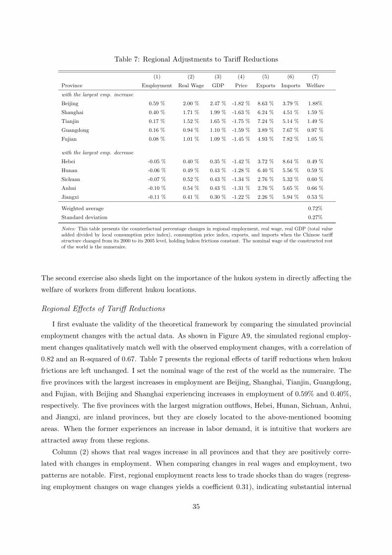
Table 7: Regional Adjustments to Tariff Reductions

(1) (2) (3) (4) (5) (6) (7)

Province Employment Real Wage GDP Price Exports Imports Welfare

with the largest emp. increase

Beijing 0.59 % 2.00 % 2.47 % -1.82 % 8.63 % 3.79 % 1.88%

Shanghai 0.40 % 1.71 % 1.99 % -1.63 % 6.24 % 4.51 % 1.59 %

Tianjin 0.17 % 1.52 % 1.65 % -1.75 % 7.24 % 5.14 % 1.49 %

Guangdong 0.16 % 0.94 % 1.10 % -1.59 % 3.89 % 7.67 % 0.97 %

Fujian 0.08 % 1.01 % 1.09 % -1.45 % 4.93 % 7.82 % 1.05 %

with the largest emp. decrease

Hebei -0.05 % 0.40 % 0.35 % -1.42 % 3.72 % 8.64 % 0.49 %

Hunan -0.06 % 0.49 % 0.43 % -1.28 % 6.40 % 5.56 % 0.59 %

Sichuan -0.07 % 0.52 % 0.43 % -1.34 % 2.76 % 5.32 % 0.60 %

Anhui -0.10 % 0.54 % 0.43 % -1.31 % 2.76 % 5.65 % 0.66 %

Jiangxi -0.11 % 0.41 % 0.30 % -1.22 % 2.26 % 5.94 % 0.53 %

Weighted average 0.72%

Standard deviation 0.27%

Notes: This table presents the counterfactual percentage changes in regional employment, real wage, real GDP (total valueadded divided by local consumption price index), consumption price index, exports, and imports when the Chinese tariffstructure changed from its 2000 to its 2005 level, holding hukou frictions constant. The nominal wage of the constructed restof the world is the numeraire.

The second exercise also sheds light on the importance of the hukou system in directly affecting the

welfare of workers from different hukou locations.

Regional Effects of Tariff Reductions

I first evaluate the validity of the theoretical framework by comparing the simulated provincial

employment changes with the actual data. As shown in Figure A9, the simulated regional employ-

ment changes qualitatively match well with the observed employment changes, with a correlation of

0.82 and an R-squared of 0.67. Table 7 presents the regional effects of tariff reductions when hukou

frictions are left unchanged. I set the nominal wage of the rest of the world as the numeraire. The

five provinces with the largest increases in employment are Beijing, Shanghai, Tianjin, Guangdong,

and Fujian, with Beijing and Shanghai experiencing increases in employment of 0.59% and 0.40%,

respectively. The five provinces with the largest migration outflows, Hebei, Hunan, Sichuan, Anhui,

and Jiangxi, are inland provinces, but they are closely located to the above-mentioned booming

areas. When the former experiences an increase in labor demand, it is intuitive that workers are

attracted away from these regions.

Column (2) shows that real wages increase in all provinces and that they are positively corre-

lated with changes in employment. When comparing changes in real wages and employment, two

patterns are notable. First, regional employment reacts less to trade shocks than do wages (regress-

ing employment changes on wage changes yields a coefficient 0.31), indicating substantial internal

35

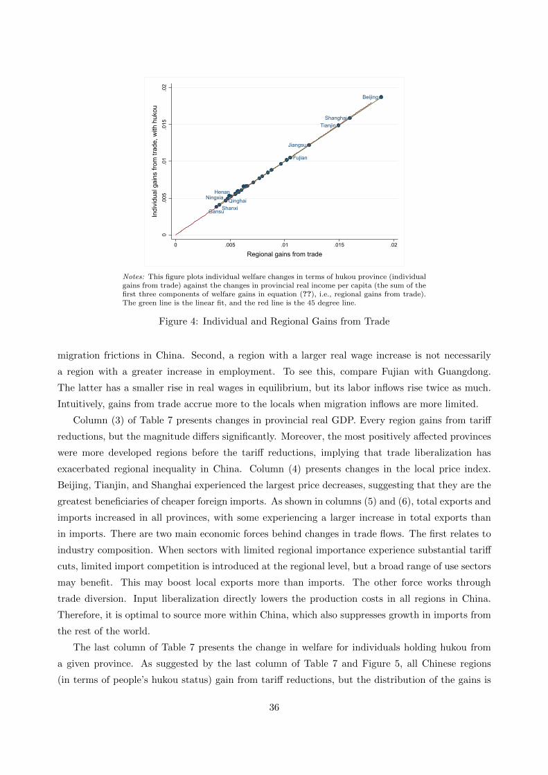
GansuShanxiQinghaiNingxia

Henan

Fujian

Jiangsu

TianjinShanghai

Beijing

0.0

05.0

1.0

15.0

2

Indi

vidu

al g

ains

from

trad

e, w

ith h

ukou

0 .005 .01 .015 .02

Regional gains from trade

Notes: This figure plots individual welfare changes in terms of hukou province (individualgains from trade) against the changes in provincial real income per capita (the sum of thefirst three components of welfare gains in equation (??), i.e., regional gains from trade).The green line is the linear fit, and the red line is the 45 degree line.

Figure 4: Individual and Regional Gains from Trade

migration frictions in China. Second, a region with a larger real wage increase is not necessarily

a region with a greater increase in employment. To see this, compare Fujian with Guangdong.

The latter has a smaller rise in real wages in equilibrium, but its labor inflows rise twice as much.

Intuitively, gains from trade accrue more to the locals when migration inflows are more limited.

Column (3) of Table 7 presents changes in provincial real GDP. Every region gains from tariff

reductions, but the magnitude differs significantly. Moreover, the most positively affected provinces

were more developed regions before the tariff reductions, implying that trade liberalization has

exacerbated regional inequality in China. Column (4) presents changes in the local price index.

Beijing, Tianjin, and Shanghai experienced the largest price decreases, suggesting that they are the

greatest beneficiaries of cheaper foreign imports. As shown in columns (5) and (6), total exports and

imports increased in all provinces, with some experiencing a larger increase in total exports than

in imports. There are two main economic forces behind changes in trade flows. The first relates to

industry composition. When sectors with limited regional importance experience substantial tariff

cuts, limited import competition is introduced at the regional level, but a broad range of use sectors

may benefit. This may boost local exports more than imports. The other force works through

trade diversion. Input liberalization directly lowers the production costs in all regions in China.

Therefore, it is optimal to source more within China, which also suppresses growth in imports from

the rest of the world.

The last column of Table 7 presents the change in welfare for individuals holding hukou from

a given province. As suggested by the last column of Table 7 and Figure 5, all Chinese regions

(in terms of people’s hukou status) gain from tariff reductions, but the distribution of the gains is

36

Table 8: Regional Effects of Hukou Abolition

(1) (2) (3) (4) (5) (6) (7)

Province Employment Real Wage GDP Price Exports Imports Welfare

with the largest emp. increase

Beijing 20.53 % -8.44 % 12.41 % -13.12 % 6.85 % -14.39 % -6.43%

Shanghai 19.39 % -8.10 % 11.93 % -13.01 % 1.30 % -14.76 % -5.87 %

Guangdong 10.42 % -4.36 % 6.94 % -12.53 % -3.84 % -13.60 % -2.93 %

Tianjin 5.87 % -2.53 % 4.01 % -11.99 % -9.00 % -12.62 % -1.46 %

Hainan 3.69 % -0.93 % 2.97 % -11.78 % -9.61 % -12.15 % -0.19 %

with the largest emp. decrease

Guangxi -2.80 % 1.64 % -1.47 % -11.44 % -16.30 % -12.18 % 2.78 %

Hunan -3.80 % 2.01 % -2.37 % -10.94 % -21.07 % -11.02 % 3.16 %

Sichuan -4.41 % 2.38 % -2.78 % -10.74 % -19.78 % -10.59 % 3.66 %

Anhui -4.47 % 2.74 % -2.38 % -11.07 % -17.84 % -11.54 % 4.10 %

Jiangxi -5.04 % 2.34 % -3.42 % -10.94 % -19.87 % -11.27 % 3.93 %

Weighted average 1.34%

Standard deviation 1.98%

Notes: This table presents the counterfactual percentage changes in regional employment, real wage, real GDP (total valueadded divided by local consumption price index), consumption price index, exports, imports, and hukou population’s welfarewhen hukou frictions are reduced to zero in all provinces, holding tariffs constant. The nominal wage of the constructed restof the world is the numeraire.

uneven. Individuals with Beijing and Shanghai hukou experience welfare improvements of 1.88% and

1.59%, respectively, while individuals holding hukou from Shanxi or Gansu province only gain 0.41%

and 0.38% – approximately 70% less. The hukou-population-weighted average welfare increase is

0.72%, with the (hukou-population-weighted) standard deviation being 0.27%.

The individual welfare in the model can be denoted as ln(Uh) = ln( yhPh

) − 1κ ln(πhh). In

other words, the labor reallocation term 1κ ln(πhh) disentangles individual gains from regional gains

(changes in regional real income) from trade. When labor is perfectly mobile, workers may choose

to move to different places due to idiosyncratic amenity draws, but the welfare changes should be

equal across individuals due to migration; when labor is perfectly immobile, the individual gains

from trade exactly equals the real income increase of the individual’s hukou province.

To explore the extent to which internal migration has alleviated the uneven welfare gains, Figure

4 plots individual welfare changes in terms of their hukou (individual gains from trade) against

the changes in provincial real income per capita (regional gains from trade). The relationship is

strikingly linear, with the data points lying around the 45 degree reference line. This suggests that

the redistribution of wealth via migration is limited: while we observe large increases in real income,

most of the gains accrue to locals due to the high costs of migration.

Effects of Tariff Reductions Given the Elimination of Hukou Frictions

Next, I examine to what extent the effects of tariff reductions can be influenced by the elimination

37

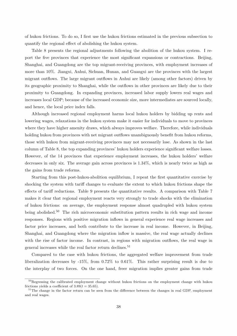
of hukou frictions. To do so, I first use the hukou frictions estimated in the previous subsection to

quantify the regional effect of abolishing the hukou system.

Table 8 presents the regional adjustments following the abolition of the hukou system. I re-

port the five provinces that experience the most significant expansions or contractions. Beijing,

Shanghai, and Guangdong are the top migrant-receiving provinces, with employment increases of

more than 10%. Jiangxi, Anhui, Sichuan, Hunan, and Guangxi are the provinces with the largest

migrant outflows. The large migrant outflows in Anhui are likely (among other factors) driven by

its geographic proximity to Shanghai, while the outflows in other provinces are likely due to their

proximity to Guangdong. In expanding provinces, increased labor supply lowers real wages and

increases local GDP; because of the increased economic size, more intermediates are sourced locally,

and hence, the local price index falls.

Although increased regional employment harms local hukou holders by bidding up rents and

lowering wages, relaxations in the hukou system make it easier for individuals to move to provinces

where they have higher amenity draws, which always improves welfare. Therefore, while individuals

holding hukou from provinces with net migrant outflows unambiguously benefit from hukou reforms,

those with hukou from migrant-receiving provinces may not necessarily lose. As shown in the last

column of Table 8, the top expanding provinces’ hukou holders experience significant welfare losses.

However, of the 14 provinces that experience employment increases, the hukou holders’ welfare

decreases in only six. The average gain across provinces is 1.34%, which is nearly twice as high as

the gains from trade reforms.

Starting from this post-hukou-abolition equilibrium, I repeat the first quantitative exercise by

shocking the system with tariff changes to evaluate the extent to which hukou frictions shape the

effects of tariff reductions. Table 9 presents the quantitative results. A comparison with Table 7

makes it clear that regional employment reacts very strongly to trade shocks with the elimination

of hukou frictions: on average, the employment response almost quadrupled with hukou system

being abolished.50 The rich microeconomic substitution pattern results in rich wage and income

responses. Regions with positive migration inflows in general experience real wage increases and

factor price increases, and both contribute to the increase in real income. However, in Beijing,

Shanghai, and Guangdong where the migration inflow is massive, the real wage actually declines

with the rise of factor income. In contrast, in regions with migration outflows, the real wage in

general increases while the real factor return declines.51

Compared to the case with hukou frictions, the aggregated welfare improvement from trade

liberalization decreases by -15%, from 0.72% to 0.61%. This rather surprising result is due to

the interplay of two forces. On the one hand, freer migration implies greater gains from trade

50Regressing the calibrated employment change without hukou frictions on the employment change with hukoufrictions yields a coefficient of 3.89(t = 35.65).

51The change in the factor return can be seen from the difference between the changes in real GDP, employmentand real wages.

38

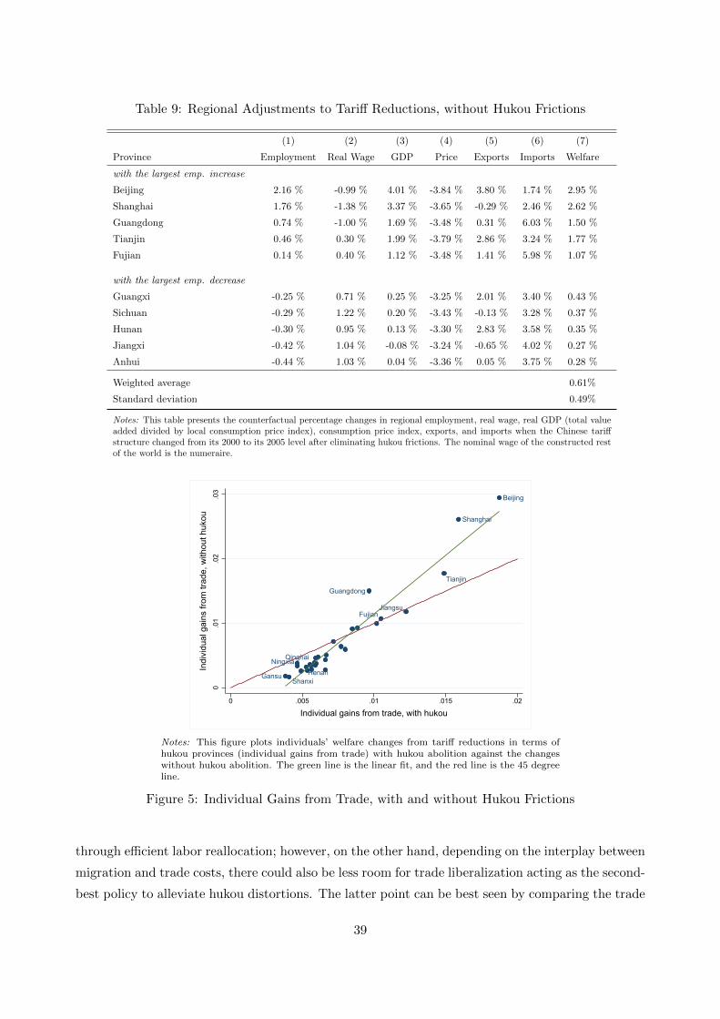
Table 9: Regional Adjustments to Tariff Reductions, without Hukou Frictions

(1) (2) (3) (4) (5) (6) (7)

Province Employment Real Wage GDP Price Exports Imports Welfare

with the largest emp. increase

Beijing 2.16 % -0.99 % 4.01 % -3.84 % 3.80 % 1.74 % 2.95 %

Shanghai 1.76 % -1.38 % 3.37 % -3.65 % -0.29 % 2.46 % 2.62 %

Guangdong 0.74 % -1.00 % 1.69 % -3.48 % 0.31 % 6.03 % 1.50 %

Tianjin 0.46 % 0.30 % 1.99 % -3.79 % 2.86 % 3.24 % 1.77 %

Fujian 0.14 % 0.40 % 1.12 % -3.48 % 1.41 % 5.98 % 1.07 %

with the largest emp. decrease

Guangxi -0.25 % 0.71 % 0.25 % -3.25 % 2.01 % 3.40 % 0.43 %

Sichuan -0.29 % 1.22 % 0.20 % -3.43 % -0.13 % 3.28 % 0.37 %

Hunan -0.30 % 0.95 % 0.13 % -3.30 % 2.83 % 3.58 % 0.35 %

Jiangxi -0.42 % 1.04 % -0.08 % -3.24 % -0.65 % 4.02 % 0.27 %

Anhui -0.44 % 1.03 % 0.04 % -3.36 % 0.05 % 3.75 % 0.28 %

Weighted average 0.61%

Standard deviation 0.49%

Notes: This table presents the counterfactual percentage changes in regional employment, real wage, real GDP (total valueadded divided by local consumption price index), consumption price index, exports, and imports when the Chinese tariffstructure changed from its 2000 to its 2005 level after eliminating hukou frictions. The nominal wage of the constructed restof the world is the numeraire.

GansuShanxi

QinghaiNingxiaHenan

Guangdong

FujianJiangsu

Tianjin

Shanghai

Beijing

0.0

1.0

2.0

3

Indi

vidu

al g

ains

from

trad

e, w

ithou

t huk

ou

0 .005 .01 .015 .02

Individual gains from trade, with hukou

Notes: This figure plots individuals’ welfare changes from tariff reductions in terms ofhukou provinces (individual gains from trade) with hukou abolition against the changeswithout hukou abolition. The green line is the linear fit, and the red line is the 45 degreeline.

Figure 5: Individual Gains from Trade, with and without Hukou Frictions

through efficient labor reallocation; however, on the other hand, depending on the interplay between

migration and trade costs, there could also be less room for trade liberalization acting as the second-

best policy to alleviate hukou distortions. The latter point can be best seen by comparing the trade

39

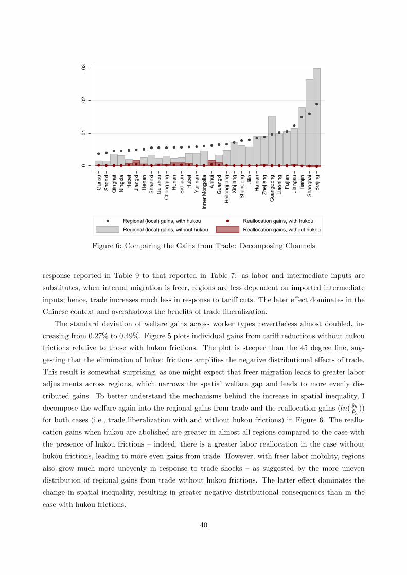
0.0

1.0

2.0

3

Gan

suSh

anxi

Qin

ghai

Nin

gxia

Heb

eiJi

angx

iH

enan

Shaa

nxi

Gui

zhou

Cho

ngqi

ngH

unan

Sich

uan

Hub

eiYu

nnan

Inne

r Mon

golia

Anhu

iG

uang

xiH

eilo

ngjia

ngXi

njia

ngSh

ando

ng Jilin

Hai

nan

Zhej

iang

Gua

ngdo

ngLi

aoni

ngFu

jian

Jian

gsu

Tian

jinSh

angh

aiBe

ijing

Regional (local) gains, with hukou Reallocation gains, with hukouRegional (local) gains, without hukou Reallocation gains, without hukou

Figure 6: Comparing the Gains from Trade: Decomposing Channels

response reported in Table 9 to that reported in Table 7: as labor and intermediate inputs are

substitutes, when internal migration is freer, regions are less dependent on imported intermediate

inputs; hence, trade increases much less in response to tariff cuts. The later effect dominates in the

Chinese context and overshadows the benefits of trade liberalization.

The standard deviation of welfare gains across worker types nevertheless almost doubled, in-

creasing from 0.27% to 0.49%. Figure 5 plots individual gains from tariff reductions without hukou

frictions relative to those with hukou frictions. The plot is steeper than the 45 degree line, sug-

gesting that the elimination of hukou frictions amplifies the negative distributional effects of trade.

This result is somewhat surprising, as one might expect that freer migration leads to greater labor

adjustments across regions, which narrows the spatial welfare gap and leads to more evenly dis-

tributed gains. To better understand the mechanisms behind the increase in spatial inequality, I

decompose the welfare again into the regional gains from trade and the reallocation gains (ln( yhPh

))

for both cases (i.e., trade liberalization with and without hukou frictions) in Figure 6. The reallo-

cation gains when hukou are abolished are greater in almost all regions compared to the case with

the presence of hukou frictions – indeed, there is a greater labor reallocation in the case without

hukou frictions, leading to more even gains from trade. However, with freer labor mobility, regions

also grow much more unevenly in response to trade shocks – as suggested by the more uneven

distribution of regional gains from trade without hukou frictions. The latter effect dominates the

change in spatial inequality, resulting in greater negative distributional consequences than in the

case with hukou frictions.

40

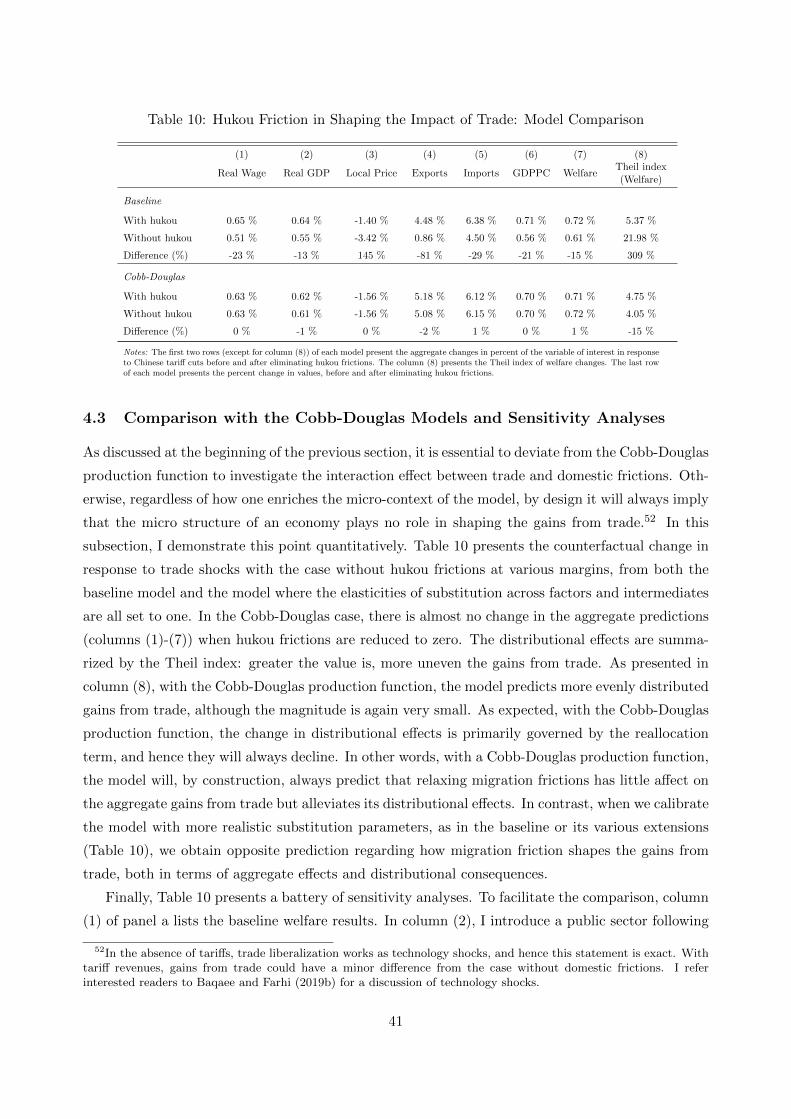
Table 10: Hukou Friction in Shaping the Impact of Trade: Model Comparison

(1) (2) (3) (4) (5) (6) (7) (8)

Real Wage Real GDP Local Price Exports Imports GDPPC WelfareTheil index(Welfare)

Baseline

With hukou 0.65 % 0.64 % -1.40 % 4.48 % 6.38 % 0.71 % 0.72 % 5.37 %

Without hukou 0.51 % 0.55 % -3.42 % 0.86 % 4.50 % 0.56 % 0.61 % 21.98 %

Difference (%) -23 % -13 % 145 % -81 % -29 % -21 % -15 % 309 %

Cobb-Douglas

With hukou 0.63 % 0.62 % -1.56 % 5.18 % 6.12 % 0.70 % 0.71 % 4.75 %

Without hukou 0.63 % 0.61 % -1.56 % 5.08 % 6.15 % 0.70 % 0.72 % 4.05 %

Difference (%) 0 % -1 % 0 % -2 % 1 % 0 % 1 % -15 %

Notes: The first two rows (except for column (8)) of each model present the aggregate changes in percent of the variable of interest in responseto Chinese tariff cuts before and after eliminating hukou frictions. The column (8) presents the Theil index of welfare changes. The last rowof each model presents the percent change in values, before and after eliminating hukou frictions.

4.3 Comparison with the Cobb-Douglas Models and Sensitivity Analyses

As discussed at the beginning of the previous section, it is essential to deviate from the Cobb-Douglas

production function to investigate the interaction effect between trade and domestic frictions. Oth-

erwise, regardless of how one enriches the micro-context of the model, by design it will always imply

that the micro structure of an economy plays no role in shaping the gains from trade.52 In this

subsection, I demonstrate this point quantitatively. Table 10 presents the counterfactual change in

response to trade shocks with the case without hukou frictions at various margins, from both the

baseline model and the model where the elasticities of substitution across factors and intermediates

are all set to one. In the Cobb-Douglas case, there is almost no change in the aggregate predictions

(columns (1)-(7)) when hukou frictions are reduced to zero. The distributional effects are summa-

rized by the Theil index: greater the value is, more uneven the gains from trade. As presented in

column (8), with the Cobb-Douglas production function, the model predicts more evenly distributed

gains from trade, although the magnitude is again very small. As expected, with the Cobb-Douglas

production function, the change in distributional effects is primarily governed by the reallocation

term, and hence they will always decline. In other words, with a Cobb-Douglas production function,

the model will, by construction, always predict that relaxing migration frictions has little affect on

the aggregate gains from trade but alleviates its distributional effects. In contrast, when we calibrate

the model with more realistic substitution parameters, as in the baseline or its various extensions

(Table 10), we obtain opposite prediction regarding how migration friction shapes the gains from

trade, both in terms of aggregate effects and distributional consequences.

Finally, Table 10 presents a battery of sensitivity analyses. To facilitate the comparison, column

(1) of panel a lists the baseline welfare results. In column (2), I introduce a public sector following

52In the absence of tariffs, trade liberalization works as technology shocks, and hence this statement is exact. Withtariff revenues, gains from trade could have a minor difference from the case without domestic frictions. I referinterested readers to Baqaee and Farhi (2019b) for a discussion of technology shocks.

41

Table 11: Alternative Model Assumptions and Parameter Values

Panel a

(1) (2) (3) (4) (5)

Baseline Hukou-benefits Local Rentiers Global Rentiers Trade Imbalances

Gains from Trade, with Hukou

Weighted Average 0.72% 0.72% 0.67% 1.74% 0.65%

Theil index 5.37% 5.37% 7.39% 2.14% 7.89%

Gains from Trade, without Hukou

Weighted Average 0.61% 0.63% 0.47% 0.57% 0.55%

Theil index 21.98% 16.04% 22.42% 12.98% 31.67%

Panel b

(1) (2) (3) (4) (5) (6) (7) (8) (9) (10)

κ = 2 κ = 4 θ0 = 1 θ0 = 7 θ1 = 3 θ1 = 7 θ2 = 3 θ2 = 7 θ3 = 1 θ3 = 5

Gains from Trade, with Hukou

Weighted Average 0.72% 0.72% 0.72% 0.72% 0.72% 0.72% 0.72% 0.72% 0.72% 0.71%

Theil index 5.76% 5.06% 5.30% 5.30% 5.81% 4.98% 5.35% 5.39% 5.34% 5.48%

Gains from Trade, without Hukou

Weighted Average 0.65% 0.58% 0.61% 0.61% 0.59% 0.64% 0.48% 0.65% 0.61% 0.61%

Theil index 15.26% 27.60% 21.88% 22.24% 35.25% 14.06% 39.63% 16.36% 22.00% 21.90%

Notes: Panel a presents the welfare effect of trade liberalization with and without hukou frictions with different model extensions. Column(1) presents the baseline results for comparison. In column (2), I introduce a public sector following Caliendo et al. (2017) and Fajgelbaumet al. (2015) and assume that migrant workers pay a higher price to access local public goods. In column (3), assume that there is amass one of rentiers in each location and that rentiers consume local goods. In column (4), I follow the literature and assume that therentiers in each location contribute rents and consume a share of the global portfolio revenue to match the observed trade imbalancesacross locations. (Caliendo et al., 2014, 2017). In column (5), compared to column (4), I instead match regional trade imbalances in theyear 2010, which I extrapolate from 2002 and 2012 regional IO tables. Panel b presents the welfare change using the same model andcounterfactual exercises as the benchmark analysis but varies one calibrated elasticity parameter at a time.

Caliendo et al. (2017) and Fajgelbaum et al. (2015) and assume that migrant workers pay a higher

price to access local public goods. In column (3), I assume that there is a mass one of rentiers

in each location and that rentiers consume local goods. In column (4), I follow the literature

and assume that the rentiers in each location contribute rents and consume a share of the global

portfolio revenue to match the observed trade imbalances across locations. (Caliendo et al., 2014,

2017). In column (5), I instead match regional trade imbalances in the year 2010, which is a linear

extrapolation based on data from 2002 and 2012 regional IO tables. The welfare implications of the

model remain qualitatively the same. Panel b of Table 10 shows that under a fairly wide range of

calibrated parameter values, the gains from trade in the presence of Hukou frictions vary between

0.71% and 0.72%. Moreover, eliminating hukou frictions reduces the gains from trade and amplifies

the negative distributional consequences in all cases. Overall, the sensitivity analyses confirm the

robustness of the quantitative results.

42

5 Conclusion

This paper shows that trade liberalization can lead to significant spatial labor adjustment within

a country, and internal migration frictions are important in shaping the impact of trade. I first

use a rich dataset on Chinese regional economies and a novel measure of hukou frictions to doc-

ument four empirical patterns that suggest input-liberalization-induced labor reallocation across

prefectures and the presence of migration frictions caused by the hukou system. Then, guided by

the empirical findings, I set up a quantitative spatial model with input-output linkages and hukou

migration frictions to estimate the welfare impact of trade liberalization and the importance of the

hukou system. The model yields tractable equations to study the regional and welfare responses to

trade shocks and a parsimonious expression linking the distributional effect of trade to the observed

change in spatial labor reallocations. Given the structure of the model, I am able to quantify the

cost of the hukou system and disentangle it from other migration costs. I find that tariff reduc-

tions improve China’s aggregate welfare by 0.72% but magnify regional disparities. Abolishing the

hukou system leads to a sizable improvement in aggregate welfare and has a strong redistributional

impact. However, it decreases the gains from trade and amplifies trade’s negative distributional

consequences. My results shed light on the importance of accounting for migration frictions when

evaluating both the aggregate and distributional consequences of trade reforms.

This paper contributes to a growing body of literature that examines the role of domestic

frictions in shaping the impact of trade liberalization, as well as the literature on trade and local

labor markets. Existing quantitative exercises typically find a weak positive interaction between

domestic frictions and trade liberalization, but I show in this paper that this result is due to the

special property of the Cobb-Douglas production function. While my focus was on China, according

to the 2013 World Population Policies (United Nations, 2013), 60 percent of governments in the

world desired a major change in their country’s spatial labor distribution, 80 percent of which had

policies to influence internal migration. This paper’s exercises could also inform migration policy

and motivate research on other countries, possibly accounting for the interaction between migration

frictions and other household characteristics.

43

References

Artuc, E., Chaudhuri, S., and McLaren, J. (2010). Trade shocks and labor adjustment: A structural

empirical approach. The American Economic Review, 100(3):1008–1045.

Artuc, E. and McLaren, J. (2012). Trade policy and wage inequality: A structural analysis with

occupational and sectoral mobility. Working Paper 18503, National Bureau of Economic Research.

Atalay, E. (2017). How important are sectoral shocks? American Economic Journal: Macroeco-

nomics, 9(4):254–80.

Autor, D. H., Dorn, D., and Hanson, G. H. (2013). The China syndrome: Local labor market effects

of import competition in the united states. The American Economic Review, 103(6):2121–2168.

Autor, D. H., Dorn, D., and Hanson, G. H. (2016). The China shock: Learning from labor-market

adjustment to large changes in trade. Annual Review of Economics, 8:205–240.

Baqaee, D. and Farhi, E. (2019a). Networks, barriers, and trade. Technical report, National Bureau

of Economic Research.

Baqaee, D. R. and Farhi, E. (2019b). The macroeconomic impact of microeconomic shocks: beyond

hulten’s theorem. Econometrica, 87(4):1155–1203.

Blancher, N. R. and Rumbaugh, T. (2004). China: International trade and WTO accession. Working

Paper 4/36, International Monetary Fund.

Boehm, C. E., Flaaen, A., and Pandalai-Nayar, N. (2019). Input linkages and the transmission of

shocks: firm-level evidence from the 2011 tohoku earthquake. Review of Economics and Statistics,

101(1):60–75.

Bosker, M., Brakman, S., Garretsen, H., and Schramm, M. (2012). Relaxing hukou: Increased labor

mobility and china’s economic geography. Journal of Urban Economics, 72(2):252–266.

Brandt, L., Van Biesebroeck, J., and Zhang, Y. (2014). Challenges of working with the Chinese

NBS firm-level data. China Economic Review, 30:339–352.

Bryan, G. and Morten, M. (2017). The aggregate productivity effects of internal migration: Evidence

from Indonesia. Working Paper 23540, National Bureau of Economic Research.

Caliendo, L., Dvorkin, M., and Parro, F. (2015). The impact of trade on labor market dynamics.

Working Paper 21149, National Bureau of Economic Research.

Caliendo, L., Opromolla, L. D., Parro, F., and Sforza, A. (2017). Goods and factor market inte-

gration: a quantitative assessment of the EU enlargement. Technical report, National Bureau of

Economic Research.

44

Caliendo, L. and Parro, F. (2015). Estimates of the trade and welfare effects of NAFTA. Review of

Economic Studies, 82(1):1–44.

Caliendo, L., Parro, F., Rossi-Hansberg, E., and Sarte, P.-D. (2014). The impact of regional and

sectoral productivity changes on the us economy. Technical report, National Bureau of Economic

Research.

Chan, K. W. (2009). The Chinese hukou system at 50. Eurasian geography and economics,

50(2):197–221.

Chan, K. W. and Buckingham, W. (2008). Is China abolishing the hukou system? The China

Quarterly, 195:582–606.

Chen, B., Lu, M., and Zhong, L. (2010). Household consumption constrained by hukou system.

Economic Research Journal, 1:62–71.

Cheng, M. (2007). How do we lose the freedom of movement: formation of China’s household

registration system in the 1950s and its evolution. Modern China Studies, 4(6):6.

Cheng, T. and Selden, M. (1994). The origins and social consequences of China’s hukou system.

The China Quarterly, 139:644–668.

Chipman, J. S. (1969). Factor price equalization and the stolper-samuelson theorem. International

Economic Review, 10(3):399–406.

Conley, T. G. and Topa, G. (2002). Socio-economic distance and spatial patterns in unemployment.

Journal of Applied Econometrics, 17(4):303–327.

Cosar, A. K. and Fajgelbaum, P. D. (2013). Internal geography, international trade, and regional

specialization. Working Paper 19697, National Bureau of Economic Research.

Dauth, W., Findeisen, S., and Suedekum, J. (2014). The rise of the East and the Far East: German

labor markets and trade integration. Journal of the European Economic Association, 12(6):1643–

1675.

Deardorff, A. V. (1994). The possibility of factor price equalization, revisited. Journal of interna-

tional Economics, 36(1-2):167–175.

Dekle, R., Eaton, J., and Kortum, S. (2008). Global rebalancing with gravity: Measuring the burden

of adjustment. IMF Staff Papers, 55(3):511–540.

Dix-Carneiro, R. (2014). Trade liberalization and labor market dynamics. Econometrica, 82(3):825–

885.

45

Dix-Carneiro, R. and Kovak, B. K. (2017). Trade liberalization and regional dynamics. American

Economic Review, 107(10):2908–2946.

Facchini, G., Liu, M. Y., Mayda, A. M., and Zhou, M. (2017). The impact of China’s WTO accession

on internal migration. Mimeo, pages 1–48.

Fajgelbaum, P. and Redding, S. J. (2014). External integration, structural transformation and

economic development: Evidence from Argentina 1870-1914. Working Paper 20217, National

Bureau of Economic Research.

Fajgelbaum, P. D., Morales, E., Serrato, J. C. S., and Zidar, O. M. (2015). State taxes and spatial

misallocation. Working Paper 21760, National Bureau of Economic Research.

Fan, H., Li, Y. A., and Yeaple, S. R. (2015). Trade liberalization, quality, and export prices. Review

of Economics and Statistics, 97(5):1033–1051.

Fan, J. (2015). Internal geography, labor mobility, and the distributional impacts of trade. Mimeo,

University of Maryland, pages 1–49.

Galle, S., Rodrıguez-Clare, A., and Yi, M. (2017). Slicing the pie: Quantifying the aggregate and

distributional effects of trade. Working Paper 23737, National Bureau of Economic Research.

Goldberg, P. K., Khandelwal, A. K., Pavcnik, N., and Topalova, P. (2010). Imported intermediate

inputs and domestic product growth: Evidence from india. The Quarterly journal of economics,

125(4):1727–1767.

Goldberg, P. K. and Pavcnik, N. (2005). Trade, wages, and the political economy of trade protection:

Evidence from the Colombian trade reforms. Journal of International Economics, 66(1):75–105.

Goldberg, P. K. and Pavcnik, N. (2007a). Distributional effects of globalization in developing

countries. Journal of economic Literature, 45(1):39–82.

Goldberg, P. K. and Pavcnik, N. (2007b). The effects of the Colombian trade liberalization on urban

poverty. In Globalization and poverty, pages 241–290. University of Chicago Press.

Grossman, G. M. and Helpman, E. (1994). Protection for sale. The American Economic Review,

84(4):833–850.

Hanson, G. H. and Slaughter, M. J. (1999). The rybczynski theorem, factor-price equalization, and

immigration: evidence from us states. Technical report, National Bureau of Economic Research.

Harrison, A., McLaren, J., and McMillan, M. (2011). Recent perspectives on trade and inequality.

Annual Review of Economics, 3(1):261–289.

46

Head, K. and Ries, J. (2001). Increasing returns versus national product differentiation as an

explanation for the pattern of US-Canada trade. American Economic Review, pages 858–876.

Herrendorf, B., Rogerson, R., and Valentinyi, A. (2013). Two perspectives on preferences and

structural transformation. American Economic Review, 103(7):2752–89.

Ianchovichina, E. and Martin, W. (2001). Trade liberalization in China’s accession to WTO. Journal

of Economic Integration, 16(4):421–445.

Kambourov, G. (2009). Labour market regulations and the sectoral reallocation of workers: The

case of trade reforms. The Review of Economic Studies, 76(4):1321–1358.

Kinnan, C., Wang, S.-Y., and Wang, Y. (2015). Relaxing migration constraints for rural households.

Working Paper 21314, National Bureau of Economic Research.

Kovak, B. K. (2011). Local labor market effects of trade policy: Evidence from Brazilian liberaliza-

tion. Mimeo, University of California, Carnegie Mellon University, pages 1–64.

Kovak, B. K. (2013). Regional effects of trade reform: What is the correct measure of liberalization?

The American Economic Review, 103(5):1960–1976.

Lardy, N. R. (1991). Foreign trade and economic reform in China, 1978-1990. Cambridge University

Press.

Lardy, N. R. (2005). Trade liberalization and its role in Chinese economic growth. In India’s and

China’s Recent Experience with Reform and Growth, pages 158–169. Springer.

Li, L. (2011). Chinese laws and regulations cleanup work lasted for 10 years without interruption.

http://cwto.mofcom.gov.cn/article/n/201109/20110907757021.shtml.

Li, Q., Junsheng, H., and Hong, D. (2001). Comparative analysis of Xiagang, the Chinese Style of

Laying Off Workers. Tsinghua University Press.

Li, X. (2013). China as a trading superpower. Mimeo, London School of Economics and Political

Science, pages 1–7.

McLaren, J. (2017). Globalization and labor market dynamics. Annual Review of Economics,

9:177–200.

McLaren, J. and Hakobyan, S. (2010). Looking for local labor market effects of NAFTA. Working

Paper 16535, National Bureau of Economic Research.

Monte, F., Redding, S. J., and Rossi-Hansberg, E. (2015). Commuting, migration and local em-

ployment elasticities. Working Paper 21706, National Bureau of Economic Research.

47

Montgomery, J. L. (2012). The inheritance of inequality: hukou and related barriers to compulsory

education for China’s migrant children. Pacific Rim Law & Policy Journal, 21:591.

Oberfield, E. and Raval, D. (2014). Micro data and macro technology. Technical report, National

Bureau of Economic Research.

Park, A., Wu, Y., and Du, Y. (2012). Informal employment in urban China. Technical report,

World Bank, Washington, DC.

Ramondo, N., Rodrıguez-Clare, A., and Saborıo-Rodrıguez, M. (2016). Trade, domestic frictions,

and scale effects. American Economic Review, 106(10):3159–84.

Redding, S. J. (2016). Goods trade, factor mobility and welfare. Journal of International Economics,

101:148 – 167.

Sun, M. and Fan, C. C. (2011). China’s permanent and temporary migrants: differentials and

changes, 1990–2000. The Professional Geographer, 63(1):92–112.

Tian, Y. (2019). International trade liberalization and domestic institutional reform. Mimeo, UCLA.

Tombe, T. and Zhu, X. (2019). Trade, migration, and productivity: A quantitative analysis of

china. American Economic Review, 109(5):1843–72.

Topalova, P. (2007). Trade liberalization, poverty and inequality: Evidence from Indian districts.

In Globalization and Poverty, pages 291–336. University of Chicago Press.

Topalova, P. (2010). Factor immobility and regional impacts of trade liberalization: Evidence on

poverty from India. American Economic Journal: Applied Economics, 2(4):1–41.

United Nations (2013). World Population Policies 2013. Technical report, United Nations, New

York, NY.

Woo, W. T. (2001). Recent claims of China’s economic exceptionalism: Reflections inspired by

WTO accession. China Economic Review, 12(2):107–136.

Wu, K., Zhang, L., and Chen, X. (2010). The barrier of hukou reform: An analysis of the qualifi-

cations for the urban hukou. Chinese Journal of Population Science, (1):66–74.

Xue, L. and Zhang, H. (2001). Shaping up sustainable urban transport authorities in China: Status

quo assessment and reforming solutions. Working paper, World Resources Institute.

48

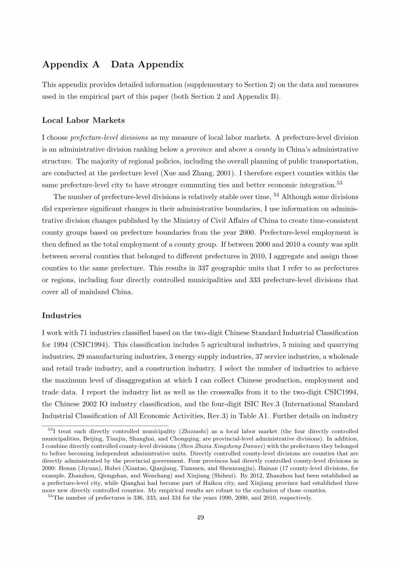
Appendix A Data Appendix

This appendix provides detailed information (supplementary to Section 2) on the data and measures

used in the empirical part of this paper (both Section 2 and Appendix B).

Local Labor Markets

I choose prefecture-level divisions as my measure of local labor markets. A prefecture-level division

is an administrative division ranking below a province and above a county in China’s administrative

structure. The majority of regional policies, including the overall planning of public transportation,

are conducted at the prefecture level (Xue and Zhang, 2001). I therefore expect counties within the

same prefecture-level city to have stronger commuting ties and better economic integration.53

The number of prefecture-level divisions is relatively stable over time, 54 Although some divisions

did experience significant changes in their administrative boundaries, I use information on adminis-

trative division changes published by the Ministry of Civil Affairs of China to create time-consistent

county groups based on prefecture boundaries from the year 2000. Prefecture-level employment is

then defined as the total employment of a county group. If between 2000 and 2010 a county was split

between several counties that belonged to different prefectures in 2010, I aggregate and assign those

counties to the same prefecture. This results in 337 geographic units that I refer to as prefectures

or regions, including four directly controlled municipalities and 333 prefecture-level divisions that

cover all of mainland China.

Industries

I work with 71 industries classified based on the two-digit Chinese Standard Industrial Classification

for 1994 (CSIC1994). This classification includes 5 agricultural industries, 5 mining and quarrying

industries, 29 manufacturing industries, 3 energy supply industries, 37 service industries, a wholesale

and retail trade industry, and a construction industry. I select the number of industries to achieve

the maximum level of disaggregation at which I can collect Chinese production, employment and

trade data. I report the industry list as well as the crosswalks from it to the two-digit CSIC1994,

the Chinese 2002 IO industry classification, and the four-digit ISIC Rev.3 (International Standard

Industrial Classification of All Economic Activities, Rev.3) in Table A1. Further details on industry

53I treat each directly controlled municipality (Zhixiashi) as a local labor market (the four directly controlledmunicipalities, Beijing, Tianjin, Shanghai, and Chongqing, are provincial-level administrative divisions). In addition,I combine directly controlled county-level divisions (Shen Zhixia Xingzheng Danwei) with the prefectures they belongedto before becoming independent administrative units. Directly controlled county-level divisions are counties that aredirectly administrated by the provincial government. Four provinces had directly controlled county-level divisions in2000: Henan (Jiyuan), Hubei (Xiantao, Qianjiang, Tianmen, and Shennongjia), Hainan (17 county-level divisions, forexample, Zhanzhou, Qiongshan, and Wenchang) and Xinjiang (Shihezi). By 2012, Zhanzhou had been established asa prefecture-level city, while Qianghai had become part of Haikou city, and Xinjiang province had established threemore new directly controlled counties. My empirical results are robust to the exclusion of those counties.

54The number of prefectures is 336, 333, and 334 for the years 1990, 2000, and 2010, respectively.

49

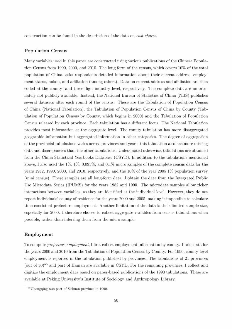
construction can be found in the description of the data on cost shares.

Population Census

Many variables used in this paper are constructed using various publications of the Chinese Popula-

tion Census from 1990, 2000, and 2010. The long form of the census, which covers 10% of the total

population of China, asks respondents detailed information about their current address, employ-

ment status, hukou, and affiliation (among others). Data on current address and affiliation are then

coded at the county- and three-digit industry level, respectively. The complete data are unfortu-

nately not publicly available. Instead, the National Bureau of Statistics of China (NBS) publishes

several datasets after each round of the census. These are the Tabulation of Population Census

of China (National Tabulation), the Tabulation of Population Census of China by County (Tab-

ulation of Population Census by County, which begins in 2000) and the Tabulation of Population

Census released by each province. Each tabulation has a different focus. The National Tabulation

provides most information at the aggregate level. The county tabulation has more disaggregated

geographic information but aggregated information in other categories. The degree of aggregation

of the provincial tabulations varies across provinces and years; this tabulation also has more missing

data and discrepancies than the other tabulations. Unless noted otherwise, tabulations are obtained

from the China Statistical Yearbooks Database (CSYD). In addition to the tabulations mentioned

above, I also used the 1%, 1%, 0.095%, and 0.1% micro samples of the complete census data for the

years 1982, 1990, 2000, and 2010, respectively, and the 10% of the year 2005 1% population survey

(mini census). These samples are all long-form data. I obtain the data from the Integrated Public

Use Microdata Series (IPUMS) for the years 1982 and 1990. The microdata samples allow richer

interactions between variables, as they are identified at the individual level. However, they do not

report individuals’ county of residence for the years 2000 and 2005, making it impossible to calculate

time-consistent prefecture employment. Another limitation of the data is their limited sample size,

especially for 2000. I therefore choose to collect aggregate variables from census tabulations when

possible, rather than inferring them from the micro sample.

Employment

To compute prefecture employment, I first collect employment information by county. I take data for

the years 2000 and 2010 from the Tabulation of Population Census by County. For 1990, county-level

employment is reported in the tabulation published by provinces. The tabulations of 21 provinces

(out of 30)55 and part of Hainan are available in CSYD. For the remaining provinces, I collect and

digitize the employment data based on paper-based publications of the 1990 tabulations. These are

available at Peking University’s Institute of Sociology and Anthropology Library.

55Chongqing was part of Sichuan province in 1990.

50

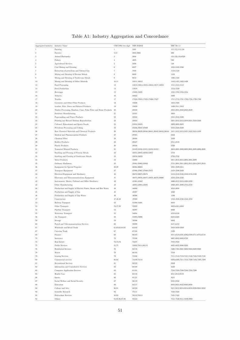
Table A1: Industry Aggregation and Concordance

Aggregated Industry Industry Name CSIC1994 two-digit NBS IO2002 ISIC Rev.3

1 Farming 1 1001 111,112,113,130

2 Forestry 2,12 2002,2003 200

3 Animal Husbandry 3 3004 121,122,150,8520

4 Fishery 4 4005 500

5 Agricultural Services 5 5006 140

6 Coal Mining and Dressing 6 6007 1010,1020,1030

7 Extraction of petroleum and Natural Gas 7 7008 1110,1120

8 Mining and Dressing of Ferrous Metals 8 8009 1310

9 Mining and Dressing of Nonferrous Metals 9 9010 1200,1320

10 Mining and Dressing of Other Minerals 10,11 10011,10012 1410,1421,1422,1429

13 Food Processing 13 13013,13014,13015,13016,13017,13018 1511,1512,1513

14 Food Production 14 13019 1514-1549

15 Beverages 15 15020,15021 1551,1552,1553,1554

16 Tobacco 16 16022 1600

17 Textiles 17 17023,17024,17025,17026,17027 1711,1712,1721,1722,1723,1729,1730

18 Garments and Other Fiber Products 18 18028 1810,1920

19 Leather, Furs, Down and Related Products 19 19029 1820,1911,1912

20 Timber Processing, Bamboo, Cane, Palm Fiber and Straw Products 20 20030 2010,2021,2022,2023,2029

21 Furniture Manufacturing 21 21031 3610

22 Papermaking and Paper Products 22 22032 2101,2102,2109

23 Printing and Record Medium Reproduction 23 23033 2211,2212,2213,2219,2221,2222,2230

24 Cultural, Educational and Sports Goods 24 24034,24035 3692,3693,3694

25 Petroleum Processing and Coking 25 25036,25037,37068 2310,2320,2330

26 Raw Chemical Materials and Chemical Products 26 26038,26039,26040,26041,26042,26043,26044 2411,2412,2413,2421,2422,2424,2429

27 Medical and Pharmaceutical Products 27 27045 2423

28 Chemical Fiber 28 28046 2430

29 Rubber Products 29 29047 2511,2519

30 Plastic Products 30 30048 2520

31 Nonmetal Mineral Products 31 31049,31050,31051,31052,31053 2610,2691,2692,2693,2694,2695,2696,2699

32 Smelting and Pressing of Ferrous Metals 32 32054,32055,32056,32057 2710

33 Smelting and Pressing of Nonferrous Metals 33 33058,33059 2720,2732

34 Metal Products 34 34060 2811,2812,2813,2892,2893,2899

35 Ordinary Machinery 35 35061,35062,35063 2731,2891,2911,2912,2913,2914,2915,2919

36 Equipment for Special Purposes 36,39 36064,36065 2921-2929,3311

37 Transport Equipment 37 37066,37067,37069,37071 3410-3599,5020

40 Electrical Equipment and Machinery 40 39072,39073,39074 3110,3120,3130,3140,3150,3190

41 Electronic and Telecommunications Equipment 41 40075,40076,40077,40078,40079,40080 3210,3220,3230

42 Instruments, Meters, Cultural and Office Machinery 42 41081,41082 3000,3312,3313,3320,3330

43 Other Manufacturing 43 42083,42084,43085 2930,3691,3699,3710,3720

44 Production and Supply of Electric Power, Steam and Hot Water 44 44086 4010,4030

45 Production and Supply of Gas 45 45087 4020

46 Production and Supply of Tap Water 46 46088 4100

47 Construction 47,48,49 47089 4510,4520,4530,4540,4550

52 Railway Transport 52 51090,51091 6010

53 Other Transport 53,57,58 52092 6023,6301,6303

54 Pipeline Transport 54 56097 6030

55 Waterway Transport 55 54094 6110,6120

56 Air Transport 56 55095,55096 6210,6220

59 Storage 59 58098 6302

60 Postal and Telecommunications Services 60 59099 6411,6412

61 Wholesale and Retail Trade 61,62,63,64,65 63102 5010,5030-5259

67 Catering Trade 67 67104 5520

68 Finance 68 68105 6511,6519,6591,6592,6599,6711,6712,6719

70 Insurance 70 70106 6601,6602,6603,6720

72 Real Estate 72,73,74 72107 7010,7020

75 Public Services 51,75 53093,79114,80115 6021,6022,9000,9233

76 Residential Services 76 82116 5260,7494,9301,9302,9303,9309,9500

78 Hotels 78 66103 5510

79 Leasing Services 79 73108 7111,7112,7113,7121,7122,7123,7129,7130

80 Commercial services 80,84 74109,74110 6304,6309,7411-7414,7430-7493,7495,7499

81 Recreational Services 81 92122 9249

82 Information and Consultative Services 82 60100 6420

83 Computer Application Services 83 61101 7210,7220,7230,7240,7250,7290

85 Health Care 85 85118 8511,8512,8519

86 Sports 86 91121 9241

87 Social Welfare and Social Security 87 86119 8531,8532

89 Education 89 84117 8010,8021,8022,8030,8090

90 Culture and Arts 90,91 88120 9211,9212,9213,9214,9219,9220,9231,9232

92 Scientific Research 92 75111 7310,7320

93 Polytechnic Services 50,93 76112,78113 7421,7422

94 Others 94,95,96,97,99 93123 7511-7530,9111-9199,9900

51

Industrial employment by county in 2000 is collected from the Tabulation of Population Census

published by each province. The data are reported in 92 two-digit CSIC1994 divisions. The original

data were collected from China Data Online; they are also available in the CSYD.56 For both

sets of data, I compared the values with those recorded in other tabulations (when available) at

various aggregations and correct mis-recorded values. When aggregating to different levels, I also

ensure that the data match the aggregated data reported in the tabulations.57 I then sum the

employment by county group to obtain the prefecture data. NBS reports 1990 employment after

sample adjustment (except for Jilin province) but not for the years 2000 or 2010. The long form

of the census is said to be randomly sampled to cover 10% of the total population. In reality,

however, sampling rates vary across regions. To avoid potential bias, I exploit the fact that the

population above the age of 15 is reported both in the full sample and in the long form. I proceed

as follows: first, I collect data by county and then calculate the sum to obtain the population of the

prefecture above age 15, from both the full sample and the long form. I then use the ratio between

the two figures to proxy for the sampling rates of each prefecture. The rates vary substantially

across prefectures, from 7.52% to 13.52% for 2000 and 7.29% to 11.50% for 2010. I finally divide

the reported employment by the constructed sampling rates to obtain the prefecture employment

for the years 2000 and 2010. Unfortunately, I do not find similar data to construct sampling rates

for 1990. I therefore simply divide the 1990 employment of Jilin province by 10%. By doing so, I

complete the final step necessary for obtaining the employment data used in my empirical analysis.

Population Measures

The data on prefecture working-age population, total population, hukou population, and the number

of migrants from other provinces in the past five years are obtained from the Tabulation of Popula-

tion Census by County. The original data are county-specific. I clean, adjust and aggregate those

variables to the prefecture level following the same procedure as used for the employment data.

Cost Shares

China became a member of the WTO on 11 December 2001. I therefore use the IO table for the

nearest year, 2002, to identify the cost shares of Chinese industries. That is, I implicitly assume that

56Unfortunately, I cannot construct a panel of employment by prefecture and sector. Both the national- and county-level tabulations report employment in aggregated industries (one-digit Chinese Standard Industrial Classification;20 sectors). Most of the employment data published by provincial administrators are by disaggregated industry(two-digit) but with inconsistencies. In 2010, Shandong only reported employment by two-digit industry by province,Chongqing reported employment by one-digit industry, and Hainan was missing data for some industries; in 1990,Liaoning reported employment by one-digit industry, and Sichuan, Shanxi, and Hunan provinces had missing data forsome industries and counties.

57When there are mis-recorded values, I cross-check the number from the provincial tabulation (when available),which also provides county-level employment for most provinces and most years; if this is not possible, I adjustthe county’s employment to be the prefecture employment minus the sum of employment of other counties in thatprefecture.

52

industry cost structures adjust slowly to trade liberalization. The 2002 IO industries are classified

in a system close to the two-digit CSIC1994, with a slightly different aggregation. For instance,

some mining and manufacturing IO divisions correspond to three-digit CSIC industries, while the

“Wholesale” division corresponds to several two-digit CSIC classifications. I therefore construct a

common industry code between IO2002 and CSIC1994 by slightly aggregating both classifications.

Ultimately, I map 122 IO and 92 CSIC divisions to 71 more aggregated industries. I then aggregate

the IO table to 71 industries and compute the cost shares.

Tariffs

I use the simple average MFN applied tariffs at the HS6 product level from the UN’s TRAINS

database to calculate tariff changes. To concord tariffs from HS6 to my constructed industry classi-

fication, I first construct a many-to-one crosswalk from ISIC Rev.3 to the constructed classification

and then use the crosswalk from HS6 to ISIC Rev.3 published by the World Integrated Trade So-

lution (WITS) to link HS6 to the classification. The final crosswalk concords HS6 products to 43

aggregated industries, spanning from agriculture to residential services. In the last step, I apply

the crosswalk to the tariff data and then take the simple average to obtain the aggregated industry

tariffs used in the empirical analysis.

Input tariffs cuts are calculated as the input-cost-weighted average of tariff reductions. To

construct external tariff reductions, I first compute the prefecture-export-weighted average of tariff

reductions that China faced from its trading partners over the 2000-2005 period for each indus-

try and each prefecture. I then take the δis-weighted average of this variable to obtain the final

prefecture measure of external tariff reductions. Exports by industry, prefecture, and destination

market are obtained by aggregating firm-level exports from the 2000 Chinese customs data. The

Chinese customs trade data cover the universe of all Chinese import and export transactions by

month; they contain the values (in US dollars) of imports and exports at the 8-digit HS classification

(approximately 7,000 product categories). The data are at the transaction level and contain firm in-

formation such as ownership (domestic, private, foreign, and state-owned), trade regime (processing

versus non-processing), and firm location. These allow me to construct bilateral trade flows between

Chinese prefectures and other countries. I exclude intermediary trade following Fan et al. (2015)

when calculating export shares; the empirical results are also robust to the exclusion of processing

exports or exports by state-owned enterprises.

Other Variables

To construct real exchange rate change by prefecture, I first compute industry-specific real exchange

rates as trade-weighted averages of real exchange rates between China and its trading partners. To

obtain the real exchange rate, I first collect countries’ nominal exchange rates with respect to the

US dollar from Penn World Table 8.1 and compute the nominal exchange rate between China and

53

Table A2: Descriptive Statistics

Variable Mean Std. Dev. Min. Max. N

Regional input tariff cuts, 2000-2005 0.03 0.01 0 0.12 337

Regional output tariff cuts, 2000-2005 0.12 0.02 0 0.20 337

Destination tariff cuts, 2000-2010 0.01 0.03 -0.11 0.23 337

Employment changes, 2000-2010 0.07 0.14 -0.36 0.66 337

Employment in 2000 14.24 0.91 10.55 16.73 337

Population changes, 2000-2010 0.07 0.12 -0.25 0.64 337

Population in 2000 14.89 0.86 11.47 17.18 337

Working age population changes, 2000-2010 0.13 0.13 -0.26 0.64 337

Working age population in 2000 14.45 0.89 10.76 16.88 337

Hukou population changes, 2000-2010 0.48 0.13 0.07 1.25 337

Hukou population in 2000 16.77 0.91 13.27 19.29 337

Changes in migration inflows, 2000-2005 versus 2005-2010 0.95 0.49 -2.22 2.38 337

Total migration inflows, 2000-2005 12.42 1.30 9.97 16.99 337

Employment changes, 1990-2000 0.11 0.18 -0.27 1.54 337

Employment in 1990 14.12 0.95 10.34 16.75 337

SOEs employment, 2000 10.80 1.20 5.35 13.76 332

SOEs employment share changes, 2000-2009 -1.09 0.76 -6.22 0.81 337

Prefecture-level exchange rates exposure, 2000-2010 0.01 0.02 -0.05 0.13 337

Share of employment in construction industry, 2000 0.03 0.02 0.001 0.09 337

Share of employment in real estate industry, 2000 0.00 0.00 0 0.03 337

Prefecture-level GDP per capita, 2000 6.46 0.72 4.20 9.50 285

Provincial hukou measure 0.53 0.28 0 1 31

Provincial hukou measure (not normalized) 0.19 0.09 0.03 0.34 31

For hukou estimation

Hukou granting dummy (obtained local hukou=1) 0.29 0.45 0 1 62260

Provincial GDP per capita, 1995 8.65 0.49 7.53 9.79 31

Rural-urban dummy (rural=1) 0.66 0.47 0 1 62260

Gender dummy (male=1) 0.5 0.5 0 1 62260

Marriage dummy (married=1) 0.58 0.50 0 1 62260

Ethnicity dummy (Han=1) 0.93 0.25 0 1 62260

Migration time 3.62 1.37 0 5 62260

Education (9 categories) 4.45 1.57 0 9 60010

ln(age) 3.15 0.57 0 4.55 61905

Notes: This table provides the descriptive statistics for variables used in the empirical analyses and for theconstruction of the hukou measure. All level variables are in logs, except birth rates, death rates, migration time, age(age and age squared), dummy variables and the categorical variable education.

other countries and then deflate the data using CPI indices from the World Bank. I then take the

change in the logged real exchange rate from 2000 to 2010 for each industry and calculate regional

exchange rate shocks as δis-weighted averages.

Employment at state-owned Enterprises (SOEs) is calculated as the total employment of indus-

trial SOEs in each prefecture. I collect the data from the NBS Annual Surveys of Industrial Firms,

which provides extensive firm-level information, including their ownership and location. The NBS

survey is particularly well suited for my analysis because all state-owned industrial firms are cov-

ered in the survey. I sum SOE employment by county for the years 2000 and 2009. I choose not to

54

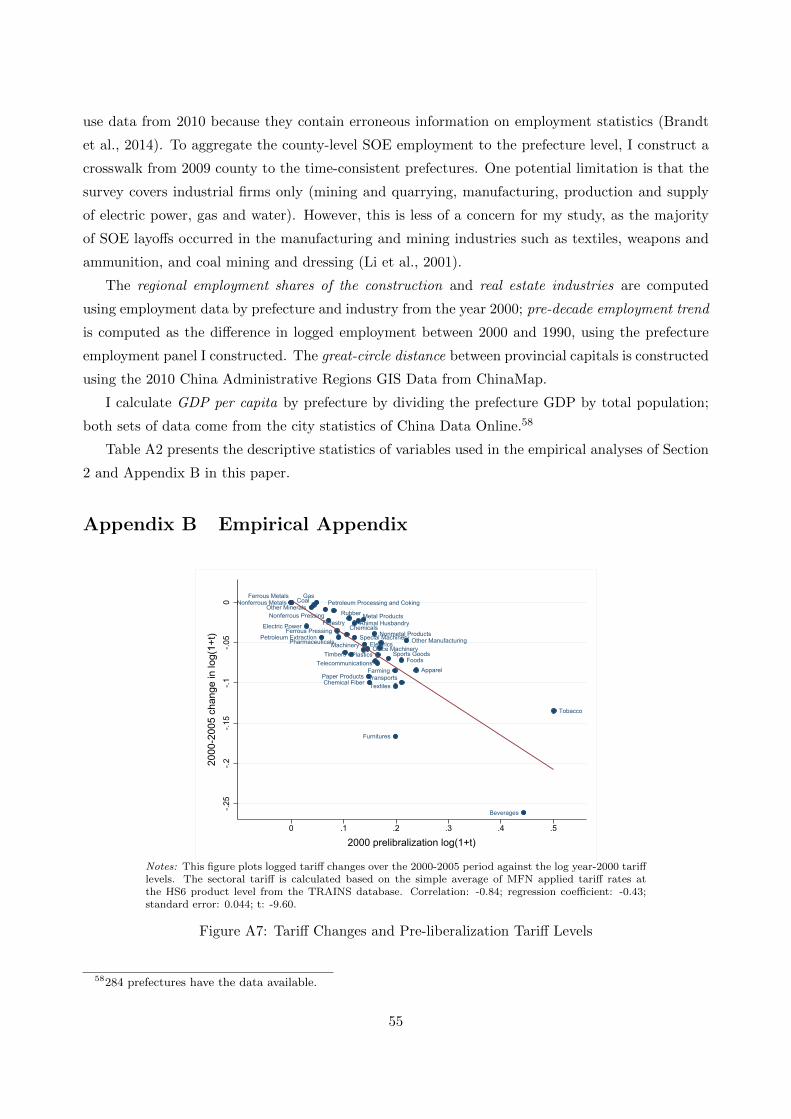
use data from 2010 because they contain erroneous information on employment statistics (Brandt

et al., 2014). To aggregate the county-level SOE employment to the prefecture level, I construct a

crosswalk from 2009 county to the time-consistent prefectures. One potential limitation is that the

survey covers industrial firms only (mining and quarrying, manufacturing, production and supply

of electric power, gas and water). However, this is less of a concern for my study, as the majority

of SOE layoffs occurred in the manufacturing and mining industries such as textiles, weapons and

ammunition, and coal mining and dressing (Li et al., 2001).

The regional employment shares of the construction and real estate industries are computed

using employment data by prefecture and industry from the year 2000; pre-decade employment trend

is computed as the difference in logged employment between 2000 and 1990, using the prefecture

employment panel I constructed. The great-circle distance between provincial capitals is constructed

using the 2010 China Administrative Regions GIS Data from ChinaMap.

I calculate GDP per capita by prefecture by dividing the prefecture GDP by total population;

both sets of data come from the city statistics of China Data Online.58

Table A2 presents the descriptive statistics of variables used in the empirical analyses of Section

2 and Appendix B in this paper.

Appendix B Empirical Appendix

Farming

Forestry Animal Husbandry

Coal

Petroleum Extraction

Ferrous MetalsNonferrous Metals

Other Minerals

Foods

Beverages

Tobacco

Textiles

Apparel

Timbers

Furnitures

Paper Products

Sports Goods

Petroleum Processing and Coking

Chemicals

Pharmaceuticals

Chemical Fiber

Rubber

Plastics

Nonmetal ProductsFerrous Pressing

Nonferrous Pressing Metal Products

MachinerySpecial Machinery

Transports

Electrics

Telecommunications

Office MachineryOther Manufacturing

Electric Power

Gas

-.25

-.2-.1

5-.1

-.05

0

2000

-200

5 ch

ange

in lo

g(1+

t)

0 .1 .2 .3 .4 .5

2000 prelibralization log(1+t)

Notes: This figure plots logged tariff changes over the 2000-2005 period against the log year-2000 tarifflevels. The sectoral tariff is calculated based on the simple average of MFN applied tariff rates atthe HS6 product level from the TRAINS database. Correlation: -0.84; regression coefficient: -0.43;standard error: 0.044; t: -9.60.

Figure A7: Tariff Changes and Pre-liberalization Tariff Levels

58284 prefectures have the data available.

55

Table A3: Relevance of Trade Flows

(a) Imports and tariffs

Import Values Unit Values Imported VarietiesAll Products Intermediates All Products Intermediates All Products Intermediates

(1) (2) (3) (4) (5) (6)

Output tariff ln(1 + tk) -2.44*** -2.22*** -0.15 0.29** -6.84*** -5.10***(0.63) (0.81) (0.12) (0.14) (1.07) (1.15)

Year FEs Yes Yes Yes Yes Yes YesHS6 FEs Yes Yes Yes YesHS6-country FEs Yes YesObservations 35,457 26,380 333,038 258,411 35,457 26,380R-squared 0.87 0.86 0.92 0.93 0.84 0.94

Notes: Columns (1) and (2) report coefficients on tariffs from HS6 product-level regressions of logged import value on logged tariffs(ln(1 + tk)), HS6 product fixed effects and year fixed effects. An observation is a HS6-year. Columns (3) and (4) regress logged unitvalue on logged tariffs, HS6-country fixed effects and year fixed effects. Unit values are computed for each HS6-country pair, and eachobservation is a HS6-country-year. Columns (5) and (6) report coefficients on tariffs from HS6 product-level regressions of the loggednumber of varieties on logged tariffs, HS6 product fixed effects, and year fixed effects. A variety is defined as an HS6-country pair, and anobservation is a HS6-year. In all regressions, tariffs are at the HS6 level. Columns (1), (3), and (5) use all products, and columns (2), (4)and (6) report coefficients for intermediates (defined according to the United Nations Broad Economic Categories (BEC) classification).Regressions are run from 2000 to 2006. Processing imports are excluded from the analysis. Robust standard errors in parentheses areclustered at the HS6 level. *** p<0.01, ** p<0.05, * p<0.1.

(b) Regional results

∆ Import Values ∆ Imported VarietiesAll Products Intermediates All Products Intermediates

(1) (2) (3) (4)

Regional input tariff cuts (∆RIT ) 28.75*** 27.57*** 10.93** 14.12***(8.47) (9.98) (4.86) (3.91)

Other Tariff Controls Yes Yes Yes YesProvince FEs Yes Yes Yes YesObservations 306 302 306 302R-squared 0.31 0.28 0.41 0.39

Notes: Columns (1) and (2) report coefficients on regional input tariff cuts from the prefecture-level regression of the loggeddifference in total imports between 2006 and 2000 on regional input tariff cuts (∆RIT ), regional output tariff reductions, externaltariff reductions, province fixed effects and logged prefecture imports in the year 2000. Columns (3) and (4) regress the loggeddifference in the number of imported varieties between 2006 and 2000 on regional input tariff cuts (∆RIT ), regional output tariffreductions, external tariff reductions, province fixed effects and the (log) number of imported varieties in the year 2000. A varietyis defined as an HS6-country pair, and an observation is a prefecture. Columns (1), (3) use all products, and columns (2), (4)report coefficients for intermediates (defined according to the United Nations Broad Economic Categories (BEC) classification).Processing imports are excluded from the analysis. Robust standard errors in parentheses are clustered at the province level. ***p<0.01, ** p<0.05, * p<0.1.

56

Notes: This figure plots the hukou measure proposed in this paper against the hukou barrier indexdeveloped by Wu et al (2010) and the hukou reform index developed by Fan (2019). To facilitate thecomparison, I translated the hukou barrier index in Wu et al (2010) using X′i = Xi −max(Xi), suchthat X′i, like my measure, is also an inverse measure of hukou frictions.

Figure A8: Comparing Hukou with Legislative-based Measure

Table A4: Effect of Input Tariff Cuts on Local Employment: Robustness I

(1) (2) (3) (4) (5) (6) (7)

Regional input tariff cuts (∆RIT ) 5.10*** 4.40** 5.14*** 3.18** 3.44** 4.45** 5.07***

(1.65) (1.89) (1.64) (1.39) (1.48) (1.63) (1.67)

Pre-liberalization employment trend 0.06

(0.09)

Changes in state-owned employment shares -0.01

(0.01)

Real exchange rate 1.26**

(0.57)

Initial share of employment, real estate 10.60***

(3.18)

Capital dummy 0.10***

(0.02)

Drop Special Economic Zones Yes

Baseline controls Yes Yes Yes Yes Yes Yes Yes

Province fixed effects Yes Yes Yes Yes Yes Yes Yes

Observations 337 337 337 337 337 337 330

R-squared 0.66 0.67 0.66 0.67 0.69 0.69 0.66

Notes: The dependent variable is the 10-year change in logged prefecture employment. The sample contains 333 prefecturesand four directly controlled municipalities. All regressions include the full vector of control variables from column (3) ofTable 1. Robust standard errors in parentheses are adjusted for 31 province clusters. Models are weighted by the log ofbeginning-of-period prefecture employment. *** p<0.01, ** p<0.05, * p<0.1.

57

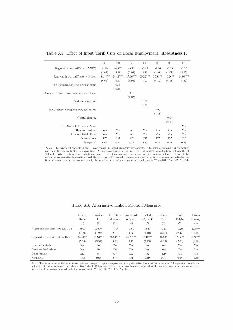
Table A5: Effect of Input Tariff Cuts on Local Employment: Robustness II

(1) (2) (3) (4) (5) (6) (7)

Regional input tariff cuts (∆RIT ) -1.18 -4.56* -0.78 -3.33 -1.86 -0.89 -0.67

(2.02) (2.40) (2.05) (2.16) (1.98) (2.01) (2.07)

Regional input tariff cuts × Hukou 18.45*** 24.13*** 17.66*** 20.22*** 15.84** 16.26** 14.90***

(6.05) (6.61) (5.94) (7.20) (6.42) (6.11) (5.32)

Pre-liberalization employment trend 0.05

(0.15)

Changes in state-owned employment shares -0.04

(0.02)

Real exchange rate 1.81

(1.43)

Initial share of employment, real estate 5.00

(5.41)

Capital dummy 0.05

(0.05)

Drop Special Economic Zones Yes

Baseline controls Yes Yes Yes Yes Yes Yes Yes

Province fixed effects Yes Yes Yes Yes Yes Yes Yes

Observations 337 337 337 337 337 337 330

R-squared 0.69 0.71 0.70 0.70 0.72 0.71 0.69

Notes: The dependent variable is the 10-year change in logged prefecture employment. The sample contains 333 prefecturesand four directly controlled municipalities. All regressions include the full vector of control variables from column (6) ofTable 1. When including each additional control, its interaction with the hukou measure is also included – none of theestimates are statistically significant and therefore are not reported. Robust standard errors in parentheses are adjusted for31 province clusters. Models are weighted by the log of beginning-of-period prefecture employment. *** p<0.01, ** p<0.05, * p<0.1.

Table A6: Alternative Hukou Friction Measures

Simple Province Prefecture Inverse s.d. Exclude Family Rural Hukou

Ratio FE Measures Weighted mig. < 30 Ties Origin Dummy

(1) (2) (3) (4) (5) (6) (7) (8)

Regional input tariff cuts (∆RIT ) -0.66 3.46** -4.30* -1.65 -2.23 -0.11 -0.20 3.85***

(2.39) (1.28) (2.15) (1.33) (2.60) (3.42) (2.47) (1.15)

Regional input tariff cuts × Hukou 15.01** 12.56*** 23.96*** 24.76*** 18.43*** 13.91* 15.96** 6.56***

(5.69) (3.55) (6.40) (4.13) (6.63) (8.14) (7.00) (1.68)

Baseline controls Yes Yes Yes Yes Yes Yes Yes Yes

Province fixed effects Yes Yes Yes Yes Yes Yes Yes Yes

Observations 337 337 337 337 337 329 335 337

R-squared 0.68 0.68 0.70 0.69 0.69 0.70 0.68 0.69

Notes: This table presents the robustness checks on changes in regional employment using alternative hukou friction measures. All regressions include thefull vector of control variables from column (6) of Table 1. Robust standard errors in parentheses are adjusted for 31 province clusters. Models are weightedby the log of beginning-of-period prefecture employment. *** p<0.01, ** p<0.05, * p<0.1.

58

Appendix C Calibration Appendix

Estimating Trade Elasticities

I calculate the sectoral trade elasticity θs based on the method developed by Caliendo and Parro

(2015). Consider three countries indexed by i, j, and n, and denote location i’s total expenditure

on varieties from sector s, location j as Xjis. Substituting equation (6) intoXijsXins

XjnsXnjs

XnisXjis

, I obtain:

Xijs

Xins

Xjns

Xnjs

Xnis

Xjis=

(τijsτins

τjnsτnjs

τnisτjis

)−θs. (A1)

Caliendo and Parro (2015) show that if iceberg trade costs τ satisfy ln(τijs) = vis + vjs + vijs + εijs,

where vijs = vjis and εijs are orthogonal to tariffs tijs, all components of τ except εijs cancel out,

and the logged trade ratio can be expressed as:

ln

(Xijs

Xins

Xjns

Xnjs

Xnis

Xjis

)= −θsln

(1 + tijs1 + tins

1 + tjns1 + tnjs

1 + tnis1 + tjis

)+ εijns, (A2)

where εijns = θs (εjis − εijs + εins − εjns + εnjs − εnis) and is orthogonal to tariffs.

I estimate the θs sector-by-sector using specification (A2) for the year 2000. I collect data on

trade flows and tariffs for 104 countries. Note that to construct the dependent variable, bilateral

trade flows between three countries all have to be non-zero. Because I am estimating θs for more

disaggregated industries than Caliendo and Parro (2015), the number of observations is limited

by the number of positive sectoral trade inflows between countries. I am also restricted by the

information on effectively applied tariff rates. Similar to Caliendo and Parro (2015), I impute the

value of some countries to increase the sample size. If a country does not have effectively applied

tariff data available in 2000, I impute this value with the closest value (in terms of date) available,

searching up to four previous years, up to 1996. When effectively applied tariffs are not available

in any of these years, I use the MFN tariffs of 2000. Data on trade flows are taken from the

UN’s Comtrade database for 2000. Values are recorded in US dollars for commodities at the HS6

product level, which I aggregate up to 43 tradable industries using concordance tables developed

in this paper. Data on tariffs are taken from TRAINS for 1996-2000 and are at the HS6 level of

disaggregation and were aggregated up to 43 tradable industries using an import-weighted average.

The total number of observations is 407,923, with 9,487 observations per sector on average.

Table A7 presents the estimated θs and heteroskedasticity-robust standard errors using the full,

99%, and 97.5% sample. The 99% and 97.5% samples were constructed by dropping small trade

flows following Caliendo and Parro (2015). The coefficients have the correct sign in most cases, and

the magnitude of the estimates varies considerably across industries.59 Two industries, mining and

dressing of ferrous metals and polytechnic services, have no variation in bilateral tariffs to identify

59The negative estimates are mainly driven by countries hit by the Asian financial crisis and China.

59

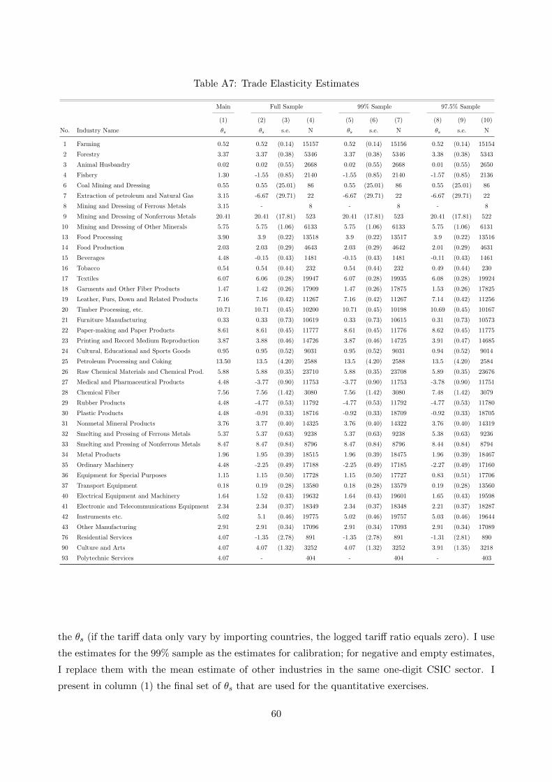
Table A7: Trade Elasticity Estimates

Main Full Sample 99% Sample 97.5% Sample

(1) (2) (3) (4) (5) (6) (7) (8) (9) (10)

No. Industry Name θs θs s.e. N θs s.e. N θs s.e. N

1 Farming 0.52 0.52 (0.14) 15157 0.52 (0.14) 15156 0.52 (0.14) 15154

2 Forestry 3.37 3.37 (0.38) 5346 3.37 (0.38) 5346 3.38 (0.38) 5343

3 Animal Husbandry 0.02 0.02 (0.55) 2668 0.02 (0.55) 2668 0.01 (0.55) 2650

4 Fishery 1.30 -1.55 (0.85) 2140 -1.55 (0.85) 2140 -1.57 (0.85) 2136

6 Coal Mining and Dressing 0.55 0.55 (25.01) 86 0.55 (25.01) 86 0.55 (25.01) 86

7 Extraction of petroleum and Natural Gas 3.15 -6.67 (29.71) 22 -6.67 (29.71) 22 -6.67 (29.71) 22

8 Mining and Dressing of Ferrous Metals 3.15 - 8 - 8 - 8

9 Mining and Dressing of Nonferrous Metals 20.41 20.41 (17.81) 523 20.41 (17.81) 523 20.41 (17.81) 522

10 Mining and Dressing of Other Minerals 5.75 5.75 (1.06) 6133 5.75 (1.06) 6133 5.75 (1.06) 6131

13 Food Processing 3.90 3.9 (0.22) 13518 3.9 (0.22) 13517 3.9 (0.22) 13516

14 Food Production 2.03 2.03 (0.29) 4643 2.03 (0.29) 4642 2.01 (0.29) 4631

15 Beverages 4.48 -0.15 (0.43) 1481 -0.15 (0.43) 1481 -0.11 (0.43) 1461

16 Tobacco 0.54 0.54 (0.44) 232 0.54 (0.44) 232 0.49 (0.44) 230

17 Textiles 6.07 6.06 (0.28) 19947 6.07 (0.28) 19935 6.08 (0.28) 19924

18 Garments and Other Fiber Products 1.47 1.42 (0.26) 17909 1.47 (0.26) 17875 1.53 (0.26) 17825

19 Leather, Furs, Down and Related Products 7.16 7.16 (0.42) 11267 7.16 (0.42) 11267 7.14 (0.42) 11256

20 Timber Processing, etc. 10.71 10.71 (0.45) 10200 10.71 (0.45) 10198 10.69 (0.45) 10167

21 Furniture Manufacturing 0.33 0.33 (0.73) 10619 0.33 (0.73) 10615 0.31 (0.73) 10573

22 Paper-making and Paper Products 8.61 8.61 (0.45) 11777 8.61 (0.45) 11776 8.62 (0.45) 11775

23 Printing and Record Medium Reproduction 3.87 3.88 (0.46) 14726 3.87 (0.46) 14725 3.91 (0.47) 14685

24 Cultural, Educational and Sports Goods 0.95 0.95 (0.52) 9031 0.95 (0.52) 9031 0.94 (0.52) 9014

25 Petroleum Processing and Coking 13.50 13.5 (4.20) 2588 13.5 (4.20) 2588 13.5 (4.20) 2584

26 Raw Chemical Materials and Chemical Prod. 5.88 5.88 (0.35) 23710 5.88 (0.35) 23708 5.89 (0.35) 23676

27 Medical and Pharmaceutical Products 4.48 -3.77 (0.90) 11753 -3.77 (0.90) 11753 -3.78 (0.90) 11751

28 Chemical Fiber 7.56 7.56 (1.42) 3080 7.56 (1.42) 3080 7.48 (1.42) 3079

29 Rubber Products 4.48 -4.77 (0.53) 11792 -4.77 (0.53) 11792 -4.77 (0.53) 11780

30 Plastic Products 4.48 -0.91 (0.33) 18716 -0.92 (0.33) 18709 -0.92 (0.33) 18705

31 Nonmetal Mineral Products 3.76 3.77 (0.40) 14325 3.76 (0.40) 14322 3.76 (0.40) 14319

32 Smelting and Pressing of Ferrous Metals 5.37 5.37 (0.63) 9238 5.37 (0.63) 9238 5.38 (0.63) 9236

33 Smelting and Pressing of Nonferrous Metals 8.47 8.47 (0.84) 8796 8.47 (0.84) 8796 8.44 (0.84) 8794

34 Metal Products 1.96 1.95 (0.39) 18515 1.96 (0.39) 18475 1.96 (0.39) 18467

35 Ordinary Machinery 4.48 -2.25 (0.49) 17188 -2.25 (0.49) 17185 -2.27 (0.49) 17160

36 Equipment for Special Purposes 1.15 1.15 (0.50) 17728 1.15 (0.50) 17727 0.83 (0.51) 17706

37 Transport Equipment 0.18 0.19 (0.28) 13580 0.18 (0.28) 13579 0.19 (0.28) 13560

40 Electrical Equipment and Machinery 1.64 1.52 (0.43) 19632 1.64 (0.43) 19601 1.65 (0.43) 19598

41 Electronic and Telecommunications Equipment 2.34 2.34 (0.37) 18349 2.34 (0.37) 18348 2.21 (0.37) 18287

42 Instruments etc. 5.02 5.1 (0.46) 19775 5.02 (0.46) 19757 5.03 (0.46) 19644

43 Other Manufacturing 2.91 2.91 (0.34) 17096 2.91 (0.34) 17093 2.91 (0.34) 17089

76 Residential Services 4.07 -1.35 (2.78) 891 -1.35 (2.78) 891 -1.31 (2.81) 890

90 Culture and Arts 4.07 4.07 (1.32) 3252 4.07 (1.32) 3252 3.91 (1.35) 3218

93 Polytechnic Services 4.07 - 404 - 404 - 403

the θs (if the tariff data only vary by importing countries, the logged tariff ratio equals zero). I use

the estimates for the 99% sample as the estimates for calibration; for negative and empty estimates,

I replace them with the mean estimate of other industries in the same one-digit CSIC sector. I

present in column (1) the final set of θs that are used for the quantitative exercises.

60

Estimating Hukou Frictions

Table A8 provides the regression results of equation (24) and robustness checks. Column (1) reports

the baseline estimates used for estimating hukou frictions in Section 4.1. As expected, migration

flows are positively correlated with the hukou measure, meaning that people will move less between

provinces with large hukou frictions. Two provinces also tend to have larger bilateral migration

inflows if they share a common border or have a short bilateral distance.

In column (2), I further control for bilateral ethnic distance to account for any migration frictions

due to the regional difference in the ethnic mix. Following Conley and Topa (2002), I calculate the

bilateral ethnic distance as the Euclidean distance between the vector of percentages of two ethnic

groups (Han versus other) of two provinces. I use the 1% random sampled data of the 3rd Population

Census from 1982 to construct this measure to avoid any simultaneity bias. If two regions have the

same ethnic composition, this variable equals zero. The negative coefficient on this measure confirms

that migration flows will be limited if two provinces are very different in minority population shares.

In column (3), I also control for bilateral industry distance using the 1% micro sample of the 1982

census data. This measure is calculated as the Euclidean distance between the vector of employment

shares over 328 industry categories. I expect this measure to capture the reallocation frictions due

to the regional difference in the industry mix. Interestingly, the variable is positively correlated

with migration flows, suggesting that workers are more likely to migrate to a region specialized in

different industries. This might be because workers move to realize their comparative advantages.

Nevertheless, the estimated coefficient is not statistically significant.

In all cases, the coefficient on the (not normalized) hukou measure is significant at the 5% level

and has the expected positive sign. The magnitude of the estimated coefficients barely changes with

additional controls. Therefore, I use the baseline estimate to calculate income costs associated with

frictions.

61

Table A8: Quantifying Hukou Frictions

Main Robustness

(1) (2) (3)

log(Hukoup ∗Hukoui) 0.29*** 0.29*** 0.36***

(0.10) (0.10) (0.11)

Distance -1.12*** -0.88*** -0.89***

(0.20) (0.23) (0.23)

Common Border 2.20*** 2.31*** 2.33***

(0.23) (0.23) (0.23)

Ethnic Distance -0.69** -0.67**

(0.27) (0.27)

Industry Distance 1.59

(1.07)

Observations 930 930 930

R-squared 0.64 0.64 0.64

Notes: This table presents the regression results of equation (24) androbustness checks. Column (1) reports the baseline estimation used forconstructing hukou frictions in Section 4.1. In columns (2) and (3), Ifurther control for the bilateral distance in ethnic groups and industrymix. In all specifications, pair fixed effects among 8 economic regionsare included. *** p<0.01, ** p<0.05, * p<0.1.

.81

1.2

1.4

1.6

Obs

erve

d em

ploy

men

t cha

nge,

200

0-20

10

-.002 0 .002 .004 .006

Simulated employment change (L'/L)

Notes: This figure plots the actual provincial employment changes (L′/L) from 2000to 2010 against the employment changes predicted by the model. Correlation: 0.82;regression coefficient: 88.74; t: 7.52; R-squared: 0.67.

Figure A9: Calibrated and Observed Employment Changes Baseline Model

62

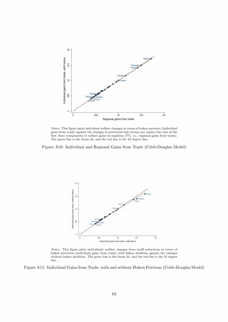
GansuShanxiQinghaiNingxia

Hebei

Fujian

Jiangsu

TianjinShanghai

Beijing

0.0

05.0

1.0

15.0

2

Indi

vidu

al g

ains

from

trad

e, w

ith h

ukou

0 .005 .01 .015 .02

Regional gains from trade

Notes: This figure plots individual welfare changes in terms of hukou province (individualgains from trade) against the changes in provincial real income per capita (the sum of thefirst three components of welfare gains in equation (??), i.e., regional gains from trade).The green line is the linear fit, and the red line is the 45 degree line.

Figure A10: Individual and Regional Gains from Trade (Cobb-Douglas Model)

Gansu ShanxiQinghai

NingxiaHenan

Fujian

JiangsuTianjin

Shanghai

Beijing

0.0

05.0

1.0

15.0

2

Indi

vidu

al g

ains

from

trad

e, w

ithou

t huk

ou

0 .005 .01 .015 .02

Individual gains from trade, with hukou

Notes: This figure plots individuals’ welfare changes from tariff reductions in terms ofhukou provinces (individual gains from trade) with hukou abolition against the changeswithout hukou abolition. The green line is the linear fit, and the red line is the 45 degreeline.

Figure A11: Individual Gains from Trade, with and without Hukou Frictions (Cobb-Douglas Model)

63