D S E Working Paper

ISSN: 1827/336X

Health, Welfare and Inequality

Gabriella BerloffaAgar BrugiaviniDino Rizzi

Dipartimento Scienze Economiche

Department of Economics

Ca’ Foscari University ofVenice

No. 41/WP/2006

W o r k i n g P a p e r s D e p a r t m e n t o f E c o n o m i c s

C a ’ F o s c a r i U n i v e r s i t y o f V e n i c e N o . 4 1 / W P / 2 0 0 6

ISSN 1827-336X

T h e W o r k i n g P a p e r S e r i e s i s a v a i l b l e o n l y o n l i n e

w w w . d s e . u n i v e . i t / p u b b l i c a z i o n i F o r e d i t o r i a l c o r r e s p o n d e n c e , p l e a s e

c o n t a c t : w p . d s e @ u n i v e . i t

D e p a r t m e n t o f E c o n o m i c s C a ’ F o s c a r i U n i v e r s i t y o f V e n i c e C a n n a r e g i o 8 7 3 , F o n d a m e n t a S a n G i o b b e 3 0 1 2 1 V e n i c e I t a l y F a x : + + 3 9 0 4 1 2 3 4 9 2 1 0

Health, Welfare and Inequality

Gabriella Berloffa University of Trento

Agar Brugiavini

University of Venice – SSAV, Scuola Studi Avanzati in Venezia

Dino Rizzi University of Venice – SSAV, Scuola Studi Avanzati in Venezia

Abstract This paper uses data from the Health and Retirement Study (HRS) to study the relationship between health status and economic welfare at household level. We develop a model to estimate the welfare cost of ill health by exploiting the methodology of the equivalence scales. The crucial variables in this approach are, besides the health status (measured in several dimensions), the economic decisions of the household which can be directly related to health conditions, such as health-related expenses. By estimating a demand system we derive health-equivalence scales to learn about the cost of health conditions on economic welfare, controlling for other covariates. Our estimates suggest that – when taking account of health – the welfare of households in poor health drops substantially and inequality increases. There are important social welfare costs associated with differences in the health status of the elderly in the USA. Keywords welfare cost, health, inequality JEL Codes I12, I31, J14

Address for correspondence: Agar Brugiavini

Department of Economics Ca’ Foscari University of Venice

Cannaregio 873, Fondamenta S.Giobbe 30121 Venezia - Italy

P h o n e : ( + + 3 9 ) 0 4 1 2 3 49162 F a x : ( + + 3 9 ) 04 1 2 3 49210

e-mail: brugiavi@unive.it

This Working Paper is published under the auspices of the Department of Economics of the Ca’ Foscari University of Venice. Opinions expressed herein are those of the authors and not those of the Department. The Working Paper series is designed to divulge preliminary or incomplete work, circulated to favour discussion and comments. Citation of this paper should consider its provisional character.

1. Introduction

This paper uses the HRS (Health and Retirement Study) to examine the

relationship between health status and economic welfare at the household

level. The terminology and the intuition go along the lines developed by the

equivalence scale literature: while in that case the focus is on the welfare

cost brought about by the presence of children, and more generally

demographics, we develop a model to estimate the welfare cost of coping

with poor health.

To this end we exploit several dimensions of households behavior available

in the HRS, which investigates different aspects of life for the ageing

population in the USA. A recent novelty of this survey is that, along with

the traditional health and socio-economic variables (CORE questionnaire), a

number of variables providing information on expenditures on various items

are also collected in a supplement (CAMS).

We cannot document paths to poverty and bad health and we cannot

investigate the direction of causality between health and economic welfare

(Smith, 1999 and 2002; Adda, Banks and von Gaudecker, 2005), because

we do not have enough waves of the data or even data linking parents and

children (Case, Lubotsky and Paxson, 2002), which would allow us to

identify some of the relevant structural parameters of this relationship.

Hence we focus the attention on the cross sectional distribution of welfare

in the sample as determined by health conditions, exploiting the (short)

panel nature of the data.

The first part of the paper is devoted to methodological issues as well as to

the definition of “health outcomes” and to the ongoing debate on health

inequality (Skinner and Zhou, 2004). The link between economic

performance and health outcomes can be investigated by making use of the

actual survival of individuals (Deaton , 2001) or of various indexes of health

conditions (Currie and Madrian, 1999, Smith 1999 and 2002, Skinner and

Zhou, 2004). The HRS offers a wide variety of health measures including

the subjective self-reported health status.

The theoretical model clarifies how health enters the indirect utility function

of the household and allows us to choose an actual measure of health which

can be assigned to each household. As for economic welfare we will follow

the tradition that recognizes income (total expenditure) as a starting point in

the measurement of well being. However, household welfare indicators

have to account for differences in demographic composition and health

conditions. Therefore we derive an ‘equivalent income’ measure of well-

being based on economic decisions of the household, which can be directly

related to health conditions, such as health-related expenses.

Our data set contains information on various expenditure categories and

medical expenditures, which we use to estimate a demand system: we argue

that these expenditures items, taken jointly, are relevant in revealing the

effects of health on welfare. The focus of the paper is the measurement of

the indirect effects of ill-health on utility implied by changes in the

structure of the cost function, hence we neglect any direct impact that

different health conditions may have on well-being.

Section 2 contains both the main set up of the model, where household

health conditions are used to derive an equivalent household income, and

some elements of the empirical implementation. Section 3 discusses

measurement issues and provides a brief description of the data, focusing

the attention on the variables of interest: health status and expenditure

measures. Section 4 presents the econometric estimates of health-related

equivalence scales, Section 5 shows the implied equivalent incomes and it

discusses the results in terms of inequality. Section 6 draws some

conclusions.

2. Health Inequality and Health Equivalence Scales- HES

There is a rich literature based on the relationship between health and

economic behaviour, investigating the well known “health-income

gradient”, but, to our knowledge, only few contributions exist on the

welfare costs of poor health conditions1.

The theoretical background is based on the notion that, at a micro level,

health enters the utility function of individuals, e.g. in the form of a stock2.

Models based on the “health-as-a-stock” assumption derive dynamic

conditions that can be analyzed and tested in a dynamic context: the

identifying strategy often hinges on unexpected shocks to health that affect

life cycle variables. One might need in this case a very long history of

health events dating back to childhood (Case, Lubotsky and Paxson, 2002;

Smith, 2002), in order to test for causality it would be necessary also to

specify the full joint data generating process for income and health (Adda,

Banks and von Gaudecker, 2005)3.

In a broader health economics perspective, several authors have addressed

the issue of “effectiveness”, i.e. how much health care spending is reflect in

better health outcomes, particularly in the USA. One strand of this literature

has looked at a more specific question: which groups in the population

account for the bulk of health care spending in a country? If it is high

income people, or more educated people, the evidence would point to

relevant socio economic disparities, which cannot be mitigated by

increasing health care spending4.

The ongoing debate on the relationship between inequality in health care

expenditures and inequality in health outcomes (and their relative strength)

obviously involves studying carefully expenditure data, the utilization of

1 See Wagstaff (1986 and 1991) and Williams (1997). Currie and Madrian (1999) provide a survey in this area of research, relating to labor supply decisions. 2 Grossman (1972a and 1972b). 3 Adda, Banks and von Gaudecker, 2005, provide a complete set up for testing the assumption that positive income innovations relate to health improvements in cohort data. 4 See for example Le Grand (1978, 1982), Le Grand et. al. (2001), Lee, McClellan and Skinner (2004) and Battacharya and Lakdawalla (2004).

effective health care and its quality (Baicker and Chandra, 2004; Skinner

and Zhou, 2004).

In this paper we focus on a micro level investigation based on a short panel

of households (Health and Retirement Study 2001 and 2003) and we

contribute to one aspect of this debate, by providing fresh evidence on the

health-income gradient based on consumption behaviour. On the basis of

our data we cannot say if the effect of ill-health on welfare can be explained

by a lack of access to care, forcing the household to bear out-of-pocket

expenses, we can however provide a coherent set of estimates of

expenditure decisions (including expenditure on health goods), conditional

on health outcomes. From these we can infer the “true” cost of health for

the sample under investigation.

In line with this approach it is appropriate to assume a static one-period

decision model where, in principle, household welfare derives from both the

utility of health and the utility of consumption. However, we do not

attempt to separately identify the direct effect of health on utility, rather our

model is based on a health-conditional cost function, from which we obtain

in turn a health-deflated level of household income. In this respect the

derivation of the demand for different commodities – including health-

related goods – follows the two-stage budgeting approach and it is

conditional on life cycle variables. In other words we measure the effects of

ill-health on the marginal valuation of the different commodities entering a

given basket.

From an empirical point of view, the concern for the endogeneity issue, i.e.

for the fact that an underlying factor – say socio-economic status – jointly

determines resources and health, is also mitigated by the fact that our health

measures are obtained from the HRS-CORE questionnaire, which is

collected one year before the HRS-CAMS, where the expenditure items are

collected. Hence health can be regarded as pre-determined vis-à-vis

expenditure choices.

In order to explain how we estimate the relationship between health and

welfare we need to specify the underlying consumer’s problem. Suppose

that each household h is characterised by a utility function defined over

household economic welfare index ( Ehy ), where E

hy will be specified as

“equivalent income” in what follows. By assuming a standard specification

of the utility function, the household welfare is:

(1) Eh

Ehh yyUv ln)( ==

Household economic welfare could depend on household demographics

(ah), on household income (yh), on commodity prices and on health status.

The household economic welfare index Ehy , is then obtained by rescaling

the actual monetary measure of income (yh) by a scale which accounts for

household characteristics s(ah) and by a scale of the health of each

household s(Hh), so that:

(2) ⎟⎟⎠

⎞⎜⎜⎝

⎛=−−==

)()(ln)(ln)(lnlnln

hh

hhhh

Ehh Hsas

yHsasyyv

Note that the two scales are assumed to be separable and therefore we

simply take the product of the two. Suppose that the expenditure function yh

= c(vh, p, ah, Hh) is defined by a demand system AIDS5,i.e.:

(3) )(),,(()(

),,,(ln

()(ln

))pBvHapA

HsasHapvc

Hsasy

hhhhh

hhh

hh

h +=⎟⎟⎠

⎞⎜⎜⎝

⎛=⎟

⎟⎠

⎞⎜⎜⎝

⎛

where p = [pi, i=1,…,N] is the vector of prices of commodities which have

been purchased. The two functions can be further specified as:

5 Almost Ideal Demand System, Deaton and Muellbauer (1980a, 1980b).

(4)

∑∑∑∑

∑∑∑

= == =

= ==

++

++=

N

k

L

llhkkl

N

k

M

mmhkkm

N

k

N

jjkkj

N

kkkhh

Hpap

pppHapA

1 11 1

1 1

*

10

lnln

lnln21ln),,(

ηλ

γαα

(5) ∏=

=N

kk

kppB1

0)( ββ

Note that the scale-terms only enter the function A.

We define the equivalence scales as :

(6) ∑=

=M

mmhmh aas

1)(ln λ

where ah = [amh, m=1,…,M] is the vector of household characteristics amh

for the household h (e.g..: gender of the head of the household, age of the

head of the household, geographical location, etc..), and:

(7) ∑=

=L

llhlh HHs

1λ)(ln

where Hh = [Hlh, l=1,…,L] is the vector of health outcomes Hlh for

household h.

By taking the derivatives of equation (7) with respect to ln pi we obtain the

budget share for the i-th commodity:

(8)

[ ] ( ) ( ) lh

L

llilimh

M

mmimi

jhhijijiih HaPypw ∑∑∑

==−+−+++=

11)/lnln λβλλβλβγα

where Ph=A(p,ah,Hh) is again an aggregate price index of relative prices

for household h.

Not that in the estimation we can only obtain values for the combined

coefficients:

(9) mimimi λβλθ −=

(10) liliil λβλπ −=

as functions of household’s demographic characteristics amh and health

characteristics Hlh. Therefore the estimation of the budget shares as

described in (8) does not directly deliver specific scales for each

demographic characteristic or health outcome, but a combination of

parameters. However, we could add a second stage to the estimation on the

basis of the following idea. If the terms miλ and liλ in (9) and (10) are

regarded as zero-sum deviations from the general equivalence scale (i.e. the

parameters mλ and lλ ) , then the latter can be retrieved once we know the

estimates for the parameters miθ , liπ and iβ6.

The actual implementation of the estimation procedure starting form

equation (8) requires knowledge of the price vector. Although we use the

CPI for the seven consumption categories defined above to obtain real

expenditures, the time variation of prices does not allow us to separately

identify price elasticities7 . If we apply the conventional normalization

carried out in cross sectional data, such that pi=1 and lnpi=0, the budget

shares of interest are :

(11) [ ])(ln)(lnln hhhiiih Hsasyw −−+= βα

(12) lh

L

llimh

M

mmihiiih Hayw ∑∑

==

+++=11πθβα ln

In this case we can show that by construction the general scales s(ah)

behaves as an equivalence scale with respect to characteristics ah, for a

given health status.

In fact we can take the ratio:

6 See also Patrizii and Rossi (1991). Note however that the “regressions” (10) and (11) cannot be implemented through an OLS procedure as residuals are non independent, therefore we resort to a GLS procedure in the parameter space. 7 Price indexes vary across regional areas and expenditure categories, but we have only one time lag between 2001 and 2003.

(13) ( )hhRh

hhh

hRh

hhh asHsasvHsasv

HapvcHapvc

==)()()exp()()()exp(

),,,(),,,(

where we normalize in such a way that the scale takes value one for the

reference household 1)( =Ras .

Most interesting for our exercise, given ah, s(Hh) behaves as an equivalence

scale based on health conditions, because:

(14) ( )hRhh

hhh

Rhh

hhh HsHsasvHsasv

HapvcHapvc

==)()()exp()()()exp(

),,,(),,,(

where we normalize so that 1)( =RHs for the reference health level. It is

useful in our context to define HR as the maximum value that the health

indicator can take, such that s(Hmax)=1 when health is “excellent”.

The combined equivalence scale for a generic household h depends on both

scales as follows:

(15) ( ) ),()()()()exp()()()exp(

),,,(),,,(

hhhhRRh

hhh

RRh

hhh HaSHsasHsasvHsasv

HapvcHapvc

===

3. The relationship between health and expenditure on health-

goods

This paper uses the HRS (Health and Retirement Study). The HRS is a

biennial panel starting in 1992, in the year 2000 it covered cohorts of 1947

or earlier, with approximately 20000 subjects aged 50 and over. The CAMS

were conducted in 2001 and 2003 (between CORE surveys), for the 2001

CAMS questionnaire were sent to 5000 people drawn from HRS 2000, in

2003 they were sent to 4156 of the respondents of 2001. Due to death and

other attrition problems the 2003-CAMS early release contains 3254

respondents which we linked to the 2001 respondents. A detailed

description of this supplement can be found in Hurd and Rohwedder (2005)

and in RAND (2005). We focus on the consumption section of the

supplement, the most knowledgeable person in the household is asked about

spending of the household: there are 32 consumption categories recorded,

we only make use of spending on 26 non-durable items. Also, we group

finer categories into broader categories as follows:

- Free time spending (trips, vacation, entertainment, hobbies etc..)

- Clothing

- Food (in and out)

- Transportation and vehicle services (including gasoline)

- Home repairs and maintenance – household items (including rent)

- Health related expenditures (out of pocket expenses on drugs,

medications, health services, medical supply etc.., not covered by

insurance)

- Housing services (including utilities such as electricity, water

charges etc..)

Table 1 shows the average and standard deviation of the budget shares of

these expenditure items in 2001 and 2003 together (in real terms). Some

households report expenditures on one consumption category only, these

observations are not informative for our analysis and we prefer to include

only households who have at least two non-zero expenditure items in their

budget8. Table 1 clearly shows that health-related expenditures are a

substantial fraction of household’s budget, the estimated mean share is

higher than the one observed for clothing and for transportation: a spending

pattern which is not surprising for this age group.

8 We excluded 411 observations through this selection.

Table 1 Mean Budget Share in the HRS (CAMS) 2001 and 2003

Budget Share Mean

Standard Deviation

health goods 0.1218 0.1405 food 0.1680 0.1596 house services 0.2158 0.1701 other house expenses 0.2613 0.2390 free time 0.0969 0.1273 clothing 0.0573 0.0749 transportation 0.0785 0.0956

As for the health measure, the HRS has information on subjective as well

as objective (self-reported) health measures. The former is the usual “how

are you?”9 question while the latter involves questions – in several

dimensions – which record the ability to perform activities (climbing stairs,

walking etc..) and current illnesses or health problems (hart and lung

conditions etc..). Furthermore we can rely on questions concerning

disability10, although these may not correspond to actual physical disability,

but only to an economic condition (collecting the benefit), they do provide

some valuable information about the overall health condition of the

respondent. In the empirical analysis we make use of three main health

indicators, all recorded at individual level:

(1) Subjective health, the scale goes from 1 (excellent) to 5 (very

poor), we rescale the coding between 1 and 0;

(2) Activities of Daily Living, particularly ADL3, which looks at three

main abilities (dressing, bathing and eating). The index ranges

between 0 (no limitations) and 3 (inability to perform all three

activities);

(3) Self-reported disabled.

The following Table 2 shows the distribution of the self-reported subjective

health condition, while Table 3 shows the distribution of ADL3 .

9 “Would you say your health is excellent, very good, good, fair, or poor?”

10 In the year 2000 question (H00G_R) and in 2002 (H02J_R), both from the CORE.

TABLE 2. Distribution of self-reported subjective health status

Subjective health Index

CORE 2000 %

CORE2002 %

CAMS 2001 %

CAMS 2003 %

poor (0.00) 9.52 9.19 6.73 5.71 fair (0.25) 18.81 19.92 17.26 17.68 good (0.50) 30.16 31.61 29.91 31.77 very good (0.75) 28.88 27.99 31.77 32.02 excellent (1.00) 12.64 11.29 14.33 12.82

Total 100.00 100.00 100.00 100.00 Number of observations 19572 18156 5811 5062

TABLE 3: Distribution of ADL3

ADL3 Index 2000 2002 2001 2003

0 85.89 85.83 90.19 90.30 1 7.93 7.66 6.71 6.16 2 3.74 3.99 2.39 2.75 3 2.44 2.53 0.71 0.79

Total 100.00 100.00 100.00 100.00 number of observations 19554 18167 5812 5063

While the health measure is available at the individual level, expenditure

and therefore welfare, are reported at household level. Hence we need to

define an health indicator for the household. Let Hhc represent the

subjective health of the individual C in household h (with c=1, …, C), it

can be aggregated at the household level on the basis of a ‘selfish-

behaviour’ assumption, i.e. by simply taking the average of individuals’

health:

(16) ∑=

=ΓC

c

hch H

HC 1 max

1

where Hmax represents the maximum level of health (i.e. someone in

excellent health conditions). For example, in our data this corresponds to the

value one. It is clear that the ‘selfish’ attitude is due to orthogonality

between the contribution of one’s health on total health and the level of

health of relatives in the household:

(17) max

1CHHhc

h =∂Γ∂

The geometric mean exhibits a more ‘altruistic’ attitude, however in this

paper we are mainly concerned with the overall effect on expenditure

decisions rather than capturing the cross effects of the composition of health

within the household, therefore we opt for the arithmetic mean.

Since the main point of the paper is to exploit the differences in the cost of

“health-goods” in relation to the health conditions of the household, we

motivate this study by first looking at the patterns of these covariates in the

data. In the CAMS sample about ten percent of the households do not report

any health expenditures, Table 4 shows the percentage distribution of

households with zero health expenditures by aggregated household health

status.

Table 4. Distribution of households with zero health expenditures

Aggregated household health index ( within household mean)

Percentage with No Health Expenditure

0.000 18.02 0.125 18.52 0.250 13.64 0.375 6.82 0.500 9.50 0.625 4.48 0.750 7.84 0.875 7.51 1.000 12.93 Total 9.51

This percentage is higher for households in “poor health” which seems

puzzling at first: there are several explanations for this evidence, including

the possibility that although there are positive health expenditures these are

fully covered by insurance11. In any event, mean and median budget

shares of health costs are higher for households in poor health, when taking

moments both conditional and unconditional on spending on health-goods.

Table 5. Mean and Median Budget Share on Health Goods by Health

Status

aggregated

health

index12

unconditional

median

unconditional

mean

conditional

median

conditional

mean

<0.40 0.091 0.151 0.114 0.174

≥0.40 and

<0.70

0.083 0.128 0.093 0.139

≥0.70 0.058 0.099 0.066 0.109

Spending patterns on health-related goods are obviously affected by the

existence of insurance coverage. In the HRS sample (individuals aged 50

and over) enrolment in Medicare is clearly relevant both for part A and for

part B (57% in the year 2000 participate to Medicare A, 95% of these

individuals is also covered by Medicare B). As for Medicaid approximately

8% of individuals is covered (mostly women, presumably dependent wives).

A residual fraction of the sample is covered by other insurances. However

participation to these plans does not drive to zero out-of-pocket health

expenditures, also because many covered goods and services imply a

substantial co-payment.

The stylized fact that this brief description highlights is that households in

“poor health” spend a substantially higher proportion of their budget in

health-related goods. We are confident that we can rule out a potential

11 For example through Medicare or Medicaid. 12 For simplicity we have combined the nine categories of the aggregate health index into

three main brackets on the basis of the density over these categories.

alternative explanation, i.e. that households which self- report poor health

conditions are not objectively unhealthy, but, simply because of their

perception, they will be spending more than the average on health-

commodities. I.e. one might argue that preferences and pessimism drive

both the answer to subjective health conditions and to health-related

expenditures. A simple Ordered Probit analysis of the subjective health

index on other self-reported objective measures (blood pressure, hart

condition etc..) shows a high predictive power of the battery of objective

variables13. Hence subjective health conditions determine health-related

expenditures largely on the basis of actual needs and not just on the basis of

different preferences.

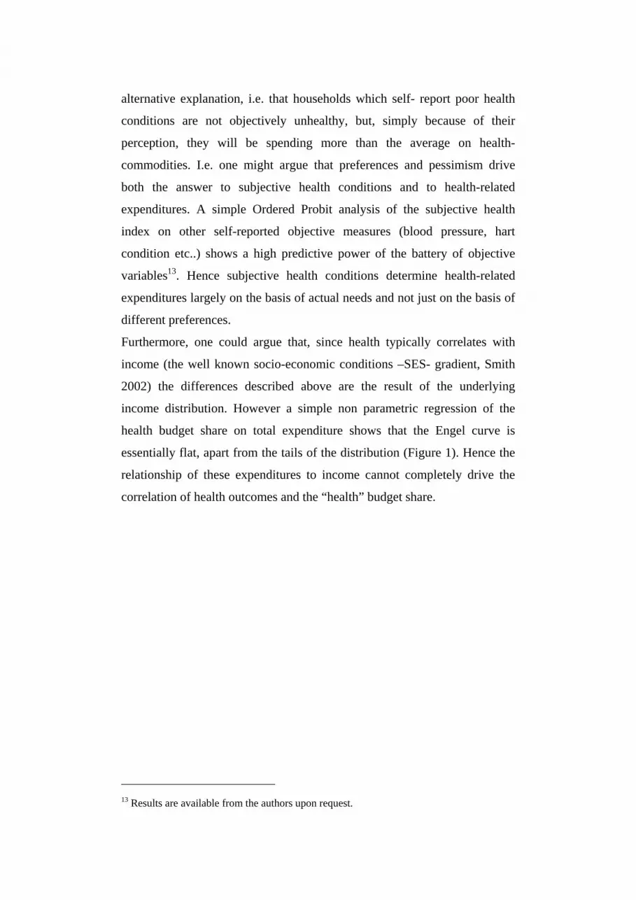
Furthermore, one could argue that, since health typically correlates with

income (the well known socio-economic conditions –SES- gradient, Smith

2002) the differences described above are the result of the underlying

income distribution. However a simple non parametric regression of the

health budget share on total expenditure shows that the Engel curve is

essentially flat, apart from the tails of the distribution (Figure 1). Hence the

relationship of these expenditures to income cannot completely drive the

correlation of health outcomes and the “health” budget share.

13 Results are available from the authors upon request.

Figure 1. Non parametric Engel curve of the “health-commodities”

budget share 0

.1.2

.3.4

6 8 10 12 14log total expenditure

lower bound upper boundmean

4. Empirical set up and results

The definition of budget shares provided in equation (13) above can be used

to estimate equivalence scales in our data. The budget share of household h

is defined over its characteristics (or characteristics of the head of the

household – such as age, or aggregation of characteristics - such as ADL).

We restrict ourselves to households with one or two-persons, because

different family compositions may imply a complex combination of health

outcomes, demographics, resources and consumption behaviour14. As we

mentioned in Section 3 we select households with non-zero expenditures on

at least two categories, the final estimation sample is described in Table A1

in the Appendix.

Demand system equations require to be simultaneously estimated: we make

use of a 3SLS procedure where the set of explanatory variables is identical

in all equations and it includes age of the head, gender of the head,

14 We also exclude a few households with missing subjective health status.

educational dummies and occupational dummies, the existence of health

insurance, health-related variables and regional dummies15.

The reason to resort to 3SLS is because we treat total expenditure as an

endogenous variable and we instrument total expenditure by a number of

instruments including income and dummies for different types of income

(see Blundell, Pashardes and Weber, 1993). In order to capture the effects

of health on budget shares we use as controls also risk factors such as

smoking and drinking habits, in fact inequality may result simply from

differences in healthy living. Furthermore we control for the presence of

medical insurance by introducing a dummy if participating Medicare, a

dummy for Medicaid and a dummy for other Medical Insurances. In this set

up the reference categories of dummy variables (or discrete variables) are

relevant to construct equivalent incomes, in particular for health the

reference category is Hmax (household health-level index between 0.7 and

1). For the other variables we choose a household whose members are

couple, all members have secondary education and all members are in

dependent employment.

Since we are dealing with panel data, observations will not be independent;

hence we use a between-transformation in order to exploit the cross

sectional variability of interest (for example differences in demographics

between households which are fixed over time). It should be recalled that

subjective health indexes and ADL measures refer to the CORE-

questionnaire of the year prior to the expenditure decision and therefore are

predetermined in our regressions.

Results are presented in Table 6, where each column refers to one

consumption category and the rows refer to selected explanatory variables16.

15 Most dummies are defined as to show whether the relevant characteristic applies to one

member of the household (e.g. low education_1) or to both members (e.g. low

education_2). 16 One consumption category (house expenditures) is omitted because, due to the adding-up

restrictions, estimates of the parameters are automatically determined. Explanatory

variables include occupational dummies, regional dummies etc…not shown for brevity.

Log-real-expenditure has a negligible effect on the health-share, which

suggest that this commodity is neither a necessity nor a luxury. This is line

with what found in Figure 1, once we properly take account of the complete

set of consumption decisions and of demographics, there is basically no

relationship of health-related out-of-pocket expenditures to income. One

could argue that the lack of correlation is totally due to the existence of

medical insurance: however we already pointed out that people covered by

Medicare might have to face substantial out-of-pocket expenses. Indeed of

the insurance dummy variables included in the regression only Medicaid has

a negative significant effect on the budget of health commodities.

In the “health-equation”, the subjective-health aggregate index has a

significant positive effect: those who report poor health conditions tend to

spend more on health related commodities.

Other variables have a minor role in the medical expenses equation, apart

from age (positive effect), the ADL3 dummies (positive effect) and drinking

habits (negative effect). Interesting enough in our demand system

educational dummies have a significant effect only on housing services and

“free-time” expenditures, not on the health-budget share, hence our

simultaneous equation system (controlling for health) does not lend support

to the view that more educated people account for the larger fraction of

health spending in the USA17. However it should be pointed out that the

HRS sample looks at a selected group of the population, which may be not

representative of the overall spending pattern of the American population

and also has important differences in terms of educational attainments.

17 See the discussion in Skinner and Zhou (2004) and Battacharya and Lakdawalla (2004)

Table 6 Estimates of the demand system on HRS-CAMS 2001 and 2003. Based on between estimator 3SLS (Selected explanatory variables – standard errors in parentheses)

Health

Goods Food House

Services Free Time Goods

Clothing Transport

Log of Real Total Expenditure

-0.007 (0.027)

-0.022 (0.027)

-0.007 (0.033)

0.101 (0.028)

0.023 (0.015)

-0.014 (0.018)

Age 0.149 (0.028)

0.030 (0.028)

-0.063 (0.033)

-0.141 (0.029)

-0.037 (0.033)

-0.052 (0.018)

Head is Male -0.010 (0.005)

0.010 (0.005)

-0.001 (0.006)

0.016 (0.005)

-0.008 (0.002)

0.006 (0.003)

One member has low education

0.004 (0.008)

-0.003 (0.008)

0.024 (0.010)

-0.002 (0.008)

-0.004 (0.004)

-0.006 (0.005)

Both members have low education

-0.033 (0.019)

-0.007 (0.019)

-0.030 (0.023)

-0.012 (0.019)

-0.008 (0.010)

0.050 (0.012)

One member is disabled

0.018 (0.011)

-0.003 (0.011)

0.002 (0.013)

-0.006 (0.011)

-0.001 (0.006)

-0.011 (0.007)

Both members are disabled

0.009 (0.033)

-0.057 (0.033)

0.065 (0.039)

0.031 (0.033)

-0.014 (0.018)

0.016 (0.022)

Subjective health “poor health”

0.046 (0.007)

0.015 (0.007)

-0.007 (0.008)

-0.052 (0.007)

-0.006 (0.003)

-0.007 (0.004)

Subjective health “fair health”

0.025 (0.005)

0.010 (0.006)

0.027 (0.007)

-0.022 (0.006)

-0.005 (0.003)

-0.001 (0.003)

One or both members with no more than one ADL3

0.014 (0.009)

0.0006 (0.009)

0.003 (0.011)

-0.011 (0.009)

-0.007 (0.005)

-0.004 (0.006)

One or both members with more than one ADL3

0.060 (0.011)

-0.019 (0.011)

-0.006 (0.014)

-0.031 (0.012)

-0.006 (0.006)

-0.012 (0.007)

Medicare dummy

-0.003 (0.007)

-0.0001 (0.007)

0.006 (0.009)

0.004 (0.007)

-0.002 (0.004)

-0.011 (0.005)

Medicaid dummy

-0.087 (0.015)

-0.016 (0.015)

0.044 (0.019)

0.038 (0.016)

0.013 (0.008)

-0.018 (0.010)

Other Insurance dummy

0.022 (0.008)

-0.023 (0.008)

0.022 (0.010)

-0.015 (0.008)

-0.009 (0.004)

0.032 (0.005)

Smoking -0.011 (0.006)

0.010 (0.006)

0.011 (0.008)

-0.023 (0.006)

-0.004 (0.003)

-0.0009 (0.004)

Drinking -0.011 (0.005)

0.006 (0.005)

-0.014 (0.006)

0.016 (0.005)

0.0008 (0.003)

-0.006 (0.003)

As for regional dummies (not shown) the West-South dummy seem to have

a positive significant effect on the health-goods budget share. Although

these dummies are just controlling for the region of residence, and not

necessarily reflecting characteristics of

the system where people receive health care (Skninner and Zhou, 2004),

when used in a demand system, along with all the other variables, these

dummies should reflect the characteristics of the supply of health care,

including differences in prices.

For the other commodities log-real expenditure has the expected sign, in

particular “free time” is positively related to “income”. No clear pattern can

be envisaged for the effect of subjective health on other commodities, apart

from “free time activities”, where the effect of ill health is negative.

Our estimates show a number of interesting facts: out-of-pocket health

expenses are strongly affected by poor health and conditions (subjective)

and by the existence of self-reported limitations in daily activities. They are

not affected by income levels or educational levels or other demographics.

The other commodity which is strongly affected by health conditions (but

also by income levels) is spending on “free time goods”. Given the age

group represented in our sample, this points to important complementarities

of these two consumption categories in households’ budgets.

5. The Implied Equivalence scales and Inequality: Beyond the Health-

Income Gradient.

The commodity-specific equivalence scales can be derived ex post, starting

from the definition provided in equations (4) and (5) and by following the

procedure described in equations (9) and (10) above, which applies a GLS

regression in the parameter space, once the estimated parameters from the

budget shares equations are known, hence delivering also a measure of

dispersion.

Once we have available health-based equivalence scales these will allow us

to study several aspects of the effects of health status which are usually

neglected in analyses of economic welfare. As we argued in the

introduction, much of the attention in the literature has focused on the direct

correlation between health and resources (income or wealth), i.e. the health

income gradient. However it is useful to measure income inequality while

controlling for health conditions, a simple extension of our econometric

analysis is to construct equivalent incomes which are based on a coherent

measure of the costs of ill health.

The health-based equivalent income( at the household level) is derived by

making use of the scale based on household subjective health conditions:

(18) )( h

hHh Hs

yy =

This represents the income that household h would need to reach its own

welfare level (given its own demographic characteristics ah), if that

household had the health status of the reference household (i.e. the

maximum health status). If the household does not enjoy excellent health,

then the equivalence scale is larger than 1 and equivalent income is below

actual money income: it is as if that household was effectively made poorer

by a lower health status. A combined equivalent income, defined by

equation (3) ca be obtained as:

(19) )()( hh

hEh Hsas

yy =

where the scale based on household demographics is also used. This is the

income that household h would need to be as well off as in its current

situation evaluated at the demographics of the reference household and at

the ‘excellent health’ status.

In all these cases equivalent income is a measure of household welfare (a

positive monotonic transformation of utility).

A simple comparison of actual income and equivalent income provides

evidence of the welfare cost of health. The distribution of this over different

characteristics (say age) also gives indications of the incidence of these

costs in different groups of the population.

For simplicity we only report equivalence scales for some relevant

dimensions in Table 7. The underlying estimates have been obtained

through the “between estimator” and by making use of real expenditure.

Table 7 shows that, other things being equal, the scale is highest (the

household is “poorest”) for the worse health conditions and is decreasing

almost linearly as health conditions get closer to their maximum value (set

equal to one).

This is a first important finding of our paper: if we consider two identical

households in terms of income (with the same total expenditure) but

different health conditions, our estimates say that the equivalent income of

the household in poor health is approximately two thirds of the equivalent

income of the healthy household. The ADL3 scale also shows a strong

effect of ill-health on welfare, implying that a relevant “compensation”

would be needed to provide such a household with the same level of welfare

as a similar household with no limitations. Age is also playing a very

important role in assessing differences in welfare: given the spending

patterns of two otherwise identical households, older households have much

lower welfare.

TABLE 7: Implied equivalence scales (based on between estimator- standard errors in

parentheses)

OLS GLS Subjective health Poor 1.495 1.621

(0.334) Fair 1.140 1.267

(0.141) Disabled One member disabled 1.046 1.042

(0.102) Both members disabled 0.661 0.806

(0.279) ADL3 One or both members with

no more than one inability 1.109 1.129

(0.077) One or both members with

more than one inability 1.289 1.274

(0.325) Single-member household

0.932 0.765 (0.105)

Age 60 1 1 70 1.246 1.211

(0.131) 80 1.508 1.428

(0.288) 90 1.784 1.653

(0.469)

Although we do not investigate the origin of these inequalities, for example

they may be explained by differential access to health care18, our

methodology correctly captures the impact of different health conditions on

household’s consumption decisions, controlling for simultaneous

consumption choices and demographics and provides a money metric

measure of the welfare loss.

Furthermore we can build on our results to ask a more general question: for

each definition of equivalent income, we can compute a standard summary

statistic of the income distribution, such as the Atkinson’s index of

inequality. If inequality increases when income is deflated by the health

18 See also Skinner and Zhou (2004)

equivalence scale, then on average poorer households are more affected by

health conditions (they tend to have poor health). In other words an increase

in inequality can be regarded as a social welfare loss due to poor health.

To construct an inequality index we start from a isoelastic welfare function:

(21) ( ) ∑= −

==−

h

h

N

h

h

hNh

UN

UUUWW1

1 11,...,,...,

1

ε

ε

where U stands for the individual utility level (which could also be

“equalised” according to one of the scales described above). For simplicity

we assume that at the individual level utility is of the simple logarithmic

form as specified in (1).

These assumptions allow us to derive an equally distributed equivalent

income: EDEY , which represents the equivalent income assigned to each

household, equally across households, such that the resulting level of total

welfare is the same as the of level of actual welfare (the latter results from

the actual income distribution). The income EDEY is a monotonic

transformation of the level of social welfare, hence it is the money metric

representation of the actual level of welfare associated with the distribution

of the equivalent household incomes. We indicate with Y the actual mean

value of the income distribution, i.e. the level of income implied by the

maximum welfare level which could be achieved given the current

resources in the economy. The Atkinson’s index of relative inequality is

then:

(22) Y

YI EDE−= 1

We can compute the Atkinson’s index for different cases of relevance to us:

for example we can look at the distribution of equivalent incomes based on

demographic scales or on health equivalence scales or both.

Table 8. Measures of inequality: equivalent incomes and the Atkinson’s index. Max

possible welfare

Actual welfare (EDE)

Mean tot expenditure

EDEY Atkinson index

Inequality Aversion Parameter is ε=0 Household income 3.21 2.84 24.77 17.04 31.10% Household equivalent income (health)

3.03 2.63 20.71 13.88 32.97%

Household equivalent income (age and health)

2.34 1.91 10.39 6.75 35.07%

Household equivalent income (age, health, and ADL3)

2.32 1.89 10.21 6.59 35.42%

Inequality Aversion Parameter is ε=1 Household income 1.17 1.00 24.77 15.19 38.66% Household equivalent income (health)

1.11 0.91 20.71 12.09 41.65%

Household equivalent income (age and health)

0.85 0.54 10.39 5.61 45.99%

Household equivalent income (age, health, and ADL3)

0.84 0.53 10.21 5.49 46.25%

Note: mean annual total expenditure in the raw data is $ 21930 (expressed in 2001-$), mean expenditures have been normalised by dividing each value by the highest in the distribution and then by multiplying by 1000.

Table 8 shows an important effect of subjective health and of the combined

“age and subjective health” variation, this is even more marked accounting

for the ADL3 variables. These figures reflect the result found above, that a

household in poor health would need a substantial compensation to be as

well off as the reference household, in fact the equally distributed equivalent

income drops dramatically. This means for example, that for those

households facing health problems, welfare, measured in money metric

units, drops by 18 percentage points.

In terms of the overall distribution of welfare, i.e. for the social cost of ill

health, the inequality index grows of about two percentage points when we

account for the equivalence scale, results are quite robust to changes in the

inequality aversion parameter used in constructing the index (we present

results only for ε=0 and ε=1, the index obviously increases when the

inequality aversion increases) 19. In other words the inequality index signals

that equivalent incomes are significantly more unequally distributed than

actual incomes.

6. Conclusions

This paper provides estimates of the effect of health on welfare by

specifying a demand system on HRS data, a sample based on the population

aged 50 and over in the U.S.A.. We use both the CORE questionnaire

(mainly for the health variables) and the CAMS questionnaire (for the

household budget), to cover the years 2001 and 2003. We specify seven

broad commodities, including “health-expenditure”, food, “free- time

expenditure” etc...

Our model adopts the two-stage budgeting approach, so that estimates of the

demand system parameters are conditional on life cycle variables.

Furthermore health variables are coded one year before the budget

information is collected – hence we can argue that health conditions are

predetermined vis-á-vis health-expenditure decisions. Our estimates show

that health expenditures are strongly affected by health conditions: ill health

is associated with a higher budget share for health related goods, after

controlling for a number of household characteristics, including age, an

ADL index, disability, education etc…

On the basis of these estimates we derive equivalence scales which suggest

that households in poor health should be “compensated” to reach the same

19 It should be recalled that the index looks at the overall welfare distribution and one

percentage point change is quite a large effect in this respect. In fact this “income”

distribution exhibits more inequality if more households in poor health are located at the

lower tail of the distribution.

level of welfare as similar households in good health conditions. In

particular, a household facing poor health, with the same actual total

expenditure of a healthy household, would have an equivalent income

curtailed of one third because of the “true” cost of health. We obtain a

money metric measure of this reduction in welfare: “equally distributed

equivalent” incomes drop of 18 percentage points for households in poor

health.

Furthermore calculations of the inequality index based on the equally

distributed equivalent incomes show a substantial degree of overall welfare

inequality due to ill health (the Atkinson’s index grows of about two

percentage points). When coupled with growth in age the same measure

shows a more marked increase in inequality: older people in poor health

suffer important disparities when compared with the reference household.

These findings suggest important social welfare costs of the existing

differences in health conditions of the elderly population in the USA.

References

Adda, J., J. Banks and H. von Gaudecker (2005), The Impact of Income

Shocks on Health: Evidence from English Cohorts, University College,

London

Atkinson, A. (1970), On the Measurement of Inequality”, Journal of

Economic Theory, September,

Baicker, K. and A. Chandra, (2004) “Medicare Spending, the Physician

Workforce, and Beneficiaries’ Quality of Care” Health Affairs (April 7).

Battacharya, J., and D. Lakdawalla, (2004) “Does Medicare Benefit the

Poor? New Answers to an Old Question,” NBER Working Paper No. 9215

.

Blundell R. P. Pashardes and G. Weber (1993) “What do we Learn About

Consumer Demand Patterns from Micro Data?”, American Economic

Review, 83, 570-597

Case, A., D. Lubotsky and C.Paxson, (2002), Economic Status and Health

in Childhood: the Origins of the Gradient, American Economic Review, 92,

no. 5, p. 1308-34.

Currie J. and B. Madrian (1999), Health, Health Insurance and the Labor

Market, in O. Ashenfelter and D. Card (eds.) Handbook of Labor

Economics, vol. 3, p.3309-3415

Deaton A., Muellbauer J. (1980a) “An Almost Ideal Demand System”,

American Economic Review, 70, pp. 312-326.

Deaton A., Muellbauer J. (1980b) Economics and Consumer Behavior,

CUP, Cambridge.

Deaton A., (2001) Relative deprivation, inequality and mortality, NBER,

wp 8099

Grossman M. (1972a) The Demand for Health: A Theoretical and

Empirical Investigation, New York, NBER.

Grossman M. (1972b) “On the concept of Health Care and Demand for

Health”, Journal of Politica Economy, 80, 2, pp. 223-255.

Hurd M and S, Rohwedder (2005) “The Retirement Consumption Puzzle,

Anticipated and Actual Declines in Spending at Retirement”, RAND Labor

and Population WR242

Jorgenson D.W., Slesnick D.T. (1986) “Aggregate Consumer Behavior and

the Measurement of Social Welfare”, Econometrica, 58, 5, pp. 1007-1040.

Le Grand, Julian, “The Distribution of Public Expenditure: The Case of

Health Care,” Economica 45(178) (May 1978): 125-142.

Le Grand, J. (1982), The Strategy of Equality. London, George Allen &

Unwin .

Le Grand, J. (1991), “The Distribution of Health Care Revisited: A

Commentary on Wagstaff, van Doorslaer and Paci, and O’Donnell and

Propper,” Journal of Health Economics 10 - 239-245.

Lee, J., M. McClellan, and J. Skinner, (1999) “The Distributional Effects

of Medicare Expenditures,” in J. Poterba (ed.) Tax Policy and the

Economy 13

Patrizii V., Rossi N. (1991) Preferenze, prezzi relativi e redistribuzione, Il

Mulino, Bologna.

RAND (2005) RAND HRS Data Description , Version E, RAND for the

Study of Aging

Skinner J. and W. Zhou (2004) “The Measurement and Evolution of Health

Inequality”, in A.J. Auerbach, D. Card, and J.M Quigley (eds.) Poverty,

The Distribution of Income, and Public Policy. New York: Russell Sage

Foundation. (NBER Working Paper No. 10842)

Smith J. (1999) “Healthy bodies and thick wallets: the dual relationship

between health and economic status”, Journal of Economic Perspective,

13, 2, 145-166.

Smith J. (2004), Unraveling the SES Health Connection, IFS working

paper WP04/02

Wagstaff A. (1986) “The Demand for Health: a Simplified Grossman

model”, Journal of Epidemiology and Community Health, 40, pp. 1-11.

Williams A. (1997) Being reasonable about the Economics of Health,

Edward Elgar.

http://hrsonline.isr.umich.edu/meta/rand/randhrse/randhrse.pdf

Table A1. Variables used in the regression analysis, mean and standard deviation for the years 2001 and 2003 (incomes and expenditures are in dollars of the year 2001)

VARIABLE MEAN STD. DEV.

Health Goods (Budget Share) 0.1264 0.127

Food (Budget Share) 0.1686 0.123

House Services (Budget Share) 0.2112 0.148

“Free Time” (Budget Share) 0.0998 0.117

Clothing (Budget Share) 0.0563 0.065

Transportation (Budget Share) 0.0766 0.079

Logarithm of Total Real Expenditure 9.6199 0.753

Households with one member 0.4489 0.492

Head is Male 0.4649 0.496

Logarithm of Age of Head 4.2169 0.138

One Member has low education 0.1193 0.323

Both Members have low education 0.0155 0.123

One Member has high education 0.2578 0.436

Both Members have high education 0.0623 0.241

One Member is retired 0.5764 0.464

Both Members are retired 0.1550 0.335

One Member non employed, but not retired 0.2138 0.382

Both Members are non employed, but not retired 0.0011 0.029

One Member is disabled 0.0792 0.256

Both Members are disabled 0.0081 0.084

Index for “poor health” 0.2544 0.405

Index for “fair health” 0.3654 0.426 One or both members with no more than one ADL3 0.0915 0.253 One or both members with more than one ADL3 0.0525 0.207

Head has private health insurance 0.7524 0.396

Head enrolled in Medicare 0.6776 0.451

Head enrolled in Medicaid 0.0658 0.238

Head currently smoker 0.1809 0.374

Head drinking alcohol 0.5751 0.473

(continues)

VARIABLE MEAN STD. DEV.

Middle Atlantic 0.1296 0.333

East North Central 0.1707 0.373

West North Central 0.0980 0.295

South Atlantic 0.2316 0.417

East South 0.0591 0.234

West South 0.0821 0.027

Mountain 0.0543 0.022

Pacific 0.1185 0.032

Number of observations 3054