productivity and welfare

Agricultural Economics Department

Faculty Publications: Agricultural Economics

University of Nebraska - Lincoln Year

Productivity and Welfare

Lilyan E. Fulginiti∗ Richard K. Perrin†

∗Dept. of Agricultural Economics, University of Nebraska - Lincoln, [email protected]†Dept. of Agricultural Economics, University of Nebraska - Lincoln

This paper is posted at DigitalCommons@University of Nebraska - Lincoln.

http://digitalcommons.unl.edu/ageconfacpub/15

Journal of Productivity Analysis, 24, 133–155, 2005© 2005 Springer Science+Business Media, Inc. Manufactured in The Netherlands.

Productivity and Welfare�

LILYAN E. FULGINITI∗ [email protected] of Nebraska, USA

RICHARD K. PERRIN [email protected] of Nebraska, USA

Abstract

Technical change is generally characterized by a rate and biases, both evaluated forgiven producer prices. This paper examines the potential discrepancy between thisrate and the corresponding rate of consumer welfare change as measured by Allaisdistributable surplus. We postulate a general equilibrium context with various mar-ket failures (taxes, quotas, imperfect competition, and “poorly priced” commodi-ties), and use comparative statics to express the rate of welfare change in terms ofthe rate and biases of the technical change. An elementary simulation model of ataxed economy suggests that the rate of welfare change may differ from the rateof technical change by as much as 50% under plausible circumstances.

JEL Classifications: D2, D5, D6, O3

Keywords: productivity, Allias surplus, general equilibrium

The very existence of the concept of productivity change, an increase in output perinput, is due to its implications for improved human welfare. Despite this humanwelfare motivation, the productivity literature has tended to focus on the produc-tion process itself to measure productivity change.1

The limitations of focusing on the production process are evident when one con-siders that, because of the law of conservation of mass and energy, what goesinto the production process must always come out, and therefore in a fundamen-tal sense there can be no productivity change. What production theory identifiesas “technology” is the relationship between achievable combinations of selectedinputs and outputs—the selection process giving a weight of one to inputs andoutputs deemed significant to human welfare, and a weight of zero to others. Azero–one weighting system for welfare relevance is crude, but necessary for theuseful process of identifying the technological possibilities with respect to welfare-significant inputs and outputs. But a change in the production technology does

� Contribution of the University of Nebraska Agricultural Experiment Station, Lincoln, NE 68583.∗ Corresponding author.

134 FULGINITI AND PERRIN

not reveal a change in welfare because of the crudeness of this zero–one weight-ing system. While it is possible to measure local shifts in the technology with dis-tance functions or supporting hyperplanes, such production-oriented measures ofproductivity change will measure welfare change only if the implicit weights are thecorrect welfare weights, which is unlikely for a number of reasons that we specifylater.

In this paper, we explicitly relate changes in the technology set to changes inwelfare in a general equilibrium context that allows for departures from Paretooptimality. We characterize technology change in terms of the rate and biasesof the local shift of the technology set. We characterize the associated welfarechange in terms of the Allais–Debreu notion of distributable surplus. We expressthe resulting Allais index of productivity change in terms of the rate and biases oftechnical change and parameters representing market imperfections. This analysisallows us to identify the circumstances which cause divergences between the Allaiswelfare index of productivity change and the more traditional rate of technicalchange, and to assess the extent of those divergences. Divergences we identify andmeasure are those due to price distortions from taxes and subsidies, quotas, mar-ket power, “poorly-priced” commodities, and those due to price changes inducedby the change in technology.

For many empirical purposes, traditional measures such as the rate of technicalchange or total factor productivity will be adequate approximations of the welfareeffects of technical change. We provide some simulation results however, that illus-trate that the potential divergence can be as much as fifty percent in the case ofheavily taxed or subsidized sectors. In any case, the analysis here helps to clarifythe relationships between welfare, productivity and technical change, for as Hicks(1945–1946) wrote with regard to his own study of alternative welfare measures,“ . . . for the purpose of clear thinking it is necessary that the basic measuresshould be distinguished, and their relationship cleared up.”

The paper is organized as follows. In Sections 1 and 2 we present the mea-sures of technical change and welfare change, respectively. In Section 3 we developthe Allais welfare measure of technical change, we place it in the context of aclosed-economy general equilibrium and examine the comparative statics effectsof technical change. In Section 4 we extend these results to various situations ofmarket failure, and in Section 5 we present an example by simulating divergencesbetween the production-oriented vs welfare-oriented measures.

1. Measures of Technical Change

Traditionally, productivity growth is defined as the difference between the growthrates of output produced and input used.2 The underlying idea is that this differ-ence reflects a change in technology that allows more output to be produced froma given amount of inputs. The indicators of technical change described in this sec-tion infer technological changes from the production behavior of firms, using eithereconometric methods or index numbers. The idea underlying these measures is that

PRODUCTIVITY AND WELFARE 135

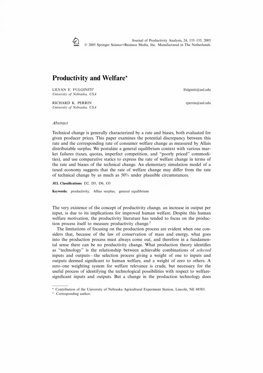
Figure 1. Welfare effects of technological change with no price distortions.

productivity growth has occurred if the cost of production of a given output hasdeclined or if profits increase for given prices.3

This literature has focused on scalar measures of the rate of change that charac-terize such changes as the one from PPF0 to PPF′ in Figure 1. In this figure thelower panel shows the numeraire good y0 on the vertical axis, the other good y


on the horizontal axis, an initial technology and initial welfare level representedby PPF0 and u0, and a subsequent technology and welfare level represented byPPF′ and u′. In the upper panel the MRS curves (Hicksian demand schedules) areslopes of the respective indifference curves in the lower panel, and the MRT curves(supply schedules) are slopes of the production possibility curves. The initial equi-librium at point A in the lower panel corresponds to point a in the upper panel. Ingeneral, no unique scalar value measures “the” increase in productivity, so a num-ber of such scalar measures have been proposed.4 The commonly-used measure ofthe rate of technical change which we adopt here is that of Samuelson, Dixit andNorman, Woodland, Diewert and Morrison, and others. It is the relative change inmaximum variable profits for a given set of prices and resources, which we defineand use as have Diewert and Morrison and Diewert and Nakamura.

To derive algebraic measures of this concept of technical change, we begin withthe aggregate profit function. Given a vector of fixed resources, z, the productionsector of the economy chooses net output vector (y0,y) in its feasible productionset, (y0,y, z) ∈ T , so as to maximize profits given the vector of producer prices(1,p). It is assumed that the production set T is non-empty, closed and convex.In perfect competition, the aggregate restricted profit function represents the solu-tion to the following problem

�(1,p, z, τ )≡Maxy0y [y0 +py|(y0,y, z, τ )∈T ], (1)

where τ is a technology index, y0 is a numeraire commodity with a price of unity,y and p are vectors of non-numeraire netputs and their respective prices, z is avector of fixed resources and the optimal choice of y satisfies5

y =�p(1,p, z, τ )≡∇p�(1,p, z, τ ). (2)

Technical change6 (TC) evaluated at initial equilibrium prices p0 is7

T echnicalChange0(TC0)≡�(1,p0, z, τ ′)−�(1,p0, z, τ 0). (3)

In the two-good economy illustrated in Figure 1, TC0 corresponds to (y07 − y03)

in the lower panel and to the area cafg in the upper panel.8 This is Hicks’ Pro-ducers’ Equivalent Variation, reflecting the change in producer surplus as a resultof a technical change that shifted the economy from an initial equilibrium, eval-uating this change at initial equilibrium prices. This definition and its graphicalillustration provide an obvious parallel with the definition of Hicksian variationsmost commonly used to measure consumer surplus changes. The rate of technicalchange (δ) that is used in this paper is the derivative equivalent of this definition,as a fraction of initial profit, or δ = (d�/dτ)/�.9

The nature of technological change can be characterized by bias as well as rate,as originally suggested by Hicks. Here we use the Binswanger definition (1974) ofnetput bias as the percentage change in the share of netput in profit due to thetechnological change under constant prices, βi = dlnki/dτ , where ki = piyi/�. Itis easily shown that share-weighted biases so defined must sum to zero, and that


they may also be expressed as βi = ∇2pi,τ�/yi − δ, that is, the difference between

the rate of change of netput yi and the rate of change in profit. Thus the techno-logical change can be characterized by the rate δ plus a vector of n× 1 biases β

defined as

Bias of Technological Change ≡ β ≡ dlnk

dτ= y−1∇2

pτ�− ıδ, (4)

where y indicates a matrix with vector y displayed on the diagonal, and ı is a n×1unit vector.

With unbiased technological change under constant prices, every netput changesat the rate of technological change δ, and thus there are no changes in shares. Thisis equivalent to a homothetic shift in the technology set, which in Figure 1 corre-sponds to a radial expansion of the PPF , rather than the expansion shown, whichis biased in favor of output y and therefore biased against output y0.

For notational simplicity we henceforth suppress the vector z, with the under-standing that �(1,p, τ ) continues to represent the returns to fixed resources.

2. Partial Equilibrium Measures of Welfare Change

One of the earliest concepts for measuring welfare change is the notion of con-sumer surplus due to Dupuit and Marshall. Their approach defined surplus in thecontext of supply and demand curves in a market for the commodity subject totaxation.10 The Griliches (1957) study of the impact of hybrid corn technologywas one of the first to use this approach to empirically measure welfare effectsof an innovation. The welfare measure he used was the change in social surplus(consumer and producer surplus) in the market for corn. Many partial equilibriumstudies that followed Griliches’ examined the distribution of welfare benefits due toprocess or product innovations. Most of these studies used the Marshallian surplusnotion to evaluate the welfare impact of a research-induced supply shift. It is nowwidely accepted that Marshallian consumer surplus is deficient as a welfare mea-sure.

A more acceptable welfare measure is Hicks’ Equivalent Variation (EV). Thismeasure of the welfare effect of a change from state A to state B is the minimumamount of money that if given to consumers in state A, would permit the con-sumer to achieve the utility level of state B.11 This concept is easily represented interms of expenditure functions. If the choice (y0,y) of a representative consumer isobtained from minimizing expenditures necessary to attain a particular utility levelu given prices (1,p), then the following expenditure function represents the solu-tion to that minimization problem:

E(1, p, u)≡Miny0,y [y0 +py|u(y0,y)≥u], (5)

where y0 is the numeraire commodity with price set to unity and the optimalchoice y satisfies12

y =Ep(1,p,u)≡∇p E(1,p,u). (6)


If the technological change moved the economy from an initial equilibrium(1,p0,u0) to (1,p′,u′), then EV is defined as13

Equivalent Variation(EV)≡E(1,p0,u′)−E(1,p0,u0). (7)

In Figure 1, EV corresponds to y06 −y03 which is equal to the area caebg in theupper panel.

3. General Equilibrium Welfare-Theoretic Measure of Productivity

The partial equilibrium measures of the benefits of innovations presented in ear-lier sections are conceptually inadequate because they do not address the gainsor losses imposed on the remainder of the economy when reallocations are madeto particular consumers or in the markets for particular commodities. Also, whenthere are market failures, a production oriented measure such as TC differs from aconsumption oriented measure such as EV. To resolve these discrepancies the con-ceptual framework must be based on some type of general equilibrium analysisthat allows for price endogeneity and for departures from Pareto optimality.

The approach we propose to measuring welfare effects of an innovation has itsroots in the work of Pareto, with more recent contributions by Allais (1973, 1977)and Debreu (1931), whose work Diewert (1981) refers to as “quantity-oriented”(measuring welfare change in units of goods.) We consider this approach consistentwith the spirit of general equilibrium, where prices are not fixed but endogenous.While most of the work using these concepts, mainly by Diewert (1981, 1983), hasfocused on taxation as the cause of welfare change, we expand it to consider thewelfare gain emanating from a profit increasing innovation.

Allais defines his measure of the welfare effect of a distortion, the distributablesurplus or Allais surplus (AS), as the maximum amount of a particular good thatcould be extracted from the distorted economy and discarded, without making anyhousehold worse off than in the distorted state, while maintaining the economy inequilibrium. For a given state of the economy, such a surplus is an intuitive mea-sure of the welfare loss inherent in that state relative to a Pareto optimal alloca-tion. The Allais approach here involves comparison of an initial, pre-innovationequilibrium with a hypothetical post-innovation reference equilibrium in which allhouseholds are at the same utility level as at the initial equilibrium, but some phys-ical good has been extracted. The reference equilibrium is hypothetical in that theanalysis does not presuppose that such a reallocation would actually occur, eventhough an omniscient government might affect such a reallocation and redistrib-ute the distributable surplus in some way that is irrelevant to the measure itself.Debreu’s “coefficient of resource utilization” is based on this concept, but his dis-posable surplus is measured in terms of the basket of resources rather than anyparticular good. In the two-goods case of Figure 1, bottom panel, the Allais mea-sure in terms of numeraire surplus appears as the maximum vertical line betweenPPF′ and u0.


Consider now a general equilibrium for a closed economy in which a represen-tative consumer expenditure function and an aggregate profit function possess theusual characteristics and can be represented by

E(1,p,u)≡Miny0,y [y0 +py|u(y0,y)≥u] and

�(1,p, τ )≡Maxy0,y [y0 +py|(y0,y, z, τ )∈T ],(8)

where: y0 is netput quantity of the numeraire good, y is an n×1 vector of netputquantities of other goods, p is an n×1 vector of prices for y, z is an n×1 vectorof fixed resources, suppressed hereafter, u is the consumer’s utility function, τ is anindex of technological change, T is the feasible technology set.

The general equilibrium conditions for this closed, competitive economy requirethat consumer expenditures must equal consumer income and that commoditymarkets must clear. These general equilibrium conditions may be represented bythe following equations:

E(1.p,u)=�(1,p, τ ), (9a)

∇pE =∇p� (9b)

Subscripts represent partial derivatives, both the producer and consumer price ofthe numeraire good must equal one, and there are n relative prices and the utilitylevel u to be determined by these n+1 equations.

First we wish to consider a “once and for all” exogenous shock to this systemin the form of a technological change from τ 0to τ ′ in a perfectly competitive econ-omy, as is illustrated for the two-good case without distortions in Figure 1. Laterwe will extend the analysis to incorporate departures from Pareto optimality. Ourmeasure of the welfare effect of this shock to the system is the Allais distributablesurplus (AS) defined as the maximum amount of numeraire commodity that couldbe extracted from the economy with the new technology while keeping consumersat the original utility level and the economy in equilibrium, or

AS=�(1,p, τ ′)−E(1,p,u0) such that∇pE(1,p,u0)=∇p�(1,p, τ ′), (10)

where expenditures and profits are measured in numeraire units (good y0), and thesupply-demand conditions are for all goods but the numeraire.14 Note that pricesare determined endogenously rather than being fixed at the pre- or post-innova-tion level.15 A casual comparison with Technical Change in equation (3) and EVin equation (7) reveals the difference between a pure production measure, a pureconsumption measure, and this general equilibrium measure.

In the two good case of Figure 1, bottom panel, the Allais measure AS appearsas the maximum vertical line between PPF′ and u0, where the slopes of the twocurves are equal, or y04 −y01. In the top panel this measure is equal to the area ofthe triangle chg.16 The reference point C, or (yr , yr

0), is a combination of goods onthe frontier of the new technology that would provide exactly the level of welfareas the initial equilibrium.


To quantify the general equilibrium welfare effects of technological change wemodify the equilibrium conditions (9) to include the Allais surplus:

E(1,p,u)+AS =�(1,p, τ ), (11a)

∇pE =∇p�. (11b)

Note that (11) is an alternative way of writing the definition in (10).To solve for the Allais surplus created by a technological change dτ , we totally

differentiate the equations in (11) and set du=0, i.e., there is to be no change inthe utility level:

∇pEdp +dAS=∇p�dp +∇τ�dτ, (12a)

∇2ppEdp =∇2

pp�dp +∇τ�dτ. (12b)

Note that because ∇pE =∇p�,dp disappears from (12a), and we can solve (12b)for the price effect of technological change

dp = (∇2ppE −∇2

pp�)−1∇2pτ�dτ (13)

which can be expressed in terms of the rate, δ and biases β, of the technologicalchange and supply and demand elasticities as

dlnp

dτ= (H −�)−1(ıδ +β), (14)

where dlnp is a vector of logarithmic price changes, H is a matrix of compen-sated demand elasticities, � is a matrix of supply elasticities, and ı is a n×1 vectorof ones.17 Note also from equation (12a) that to a first degree, the Allais welfarechange is equal to the rate of technical change.

From equation (14) it is clear that there are two sufficient conditions for theAllais surplus extraction to have no induced price effects. The first condition is thatall non-numeraire commodity biases be identical and equal to the negative of rateof technical change (−δ=βi). This implies that the bias of technical change for thenumeraire commodity is β0 = (1/k0 −1)δ. The second condition is that all prices beexogenous i.e., when the diagonal elements of the matrices � or H approach infin-ity.

Using a Taylor expansion of AS(1,p′, τ ′) from (10) about the equilibrium point(1,p0, τ 0), we obtain a second-order approximation of the AS associated with aonce and for all technological change:18

AS≈ (∇p�−∇pE)dp +∇τ�dτ

+12(dpTdτT)

[∇2ppE −∇2

pp� ∇2pτ�

∇2pτ� ∇2

pp�

](dp

dτ

)

=∇τ�dτ +dpT∇2pτ�dτ + 1

2dpT(∇2

pp�−∇2ppE)dp + 1

2dpT(∇2

ττ�)dp

=∇τ�dτ − 12∇2

pτ�(∇2pp�−∇2

ppE)−1∇2pτ�dτ, (15)


where subscripts indicate differentiation and ∇2ττ�=0. Given that the second term

of the last line of equation (15) is positive, then to a second degree approxima-tion,the measure of welfare change is at most as big as the measure of technicalchange. Dividing AS by initial expenditures E0 =E(1,p0,u0), allows us to expressAS as a fraction of initial expenditures, and (15) in terms of shares and elasticities:19

d

dτ

ASE0

≈ δ + (ıδ +β)sdlnp + (ıδ +β)Ts(� −H )dlnp

≈ δ − 12(ıδ +β)Ts(� −H )−1(ıδ +β), (16)

where s is an n×1 vector of expenditure shares, s is a diagonal matrix, and in thelast expression in (16) we have substituted the price change from equation (14).

Equation (16) is a primary analytical result of this paper, an explicit solution ofthe consumers’ potential welfare gains20 from technical change in a perfectly com-petitive economy with no market failures, as a function of the rate and bias char-acteristics of that technical change. It establishes that to the extent that there areinduced price effects, the rate of technical change δ will most likely overestimatethe welfare impact of an innovation.

4. Welfare-Theoretic Measure of Productivity Under Market Failure

We now return to the issue of the potential mistakes incurred in productivity mea-surement when market prices do not reflect the subjective valuation of consumers,due to market failure.21 As we mentioned before, the practice of focusing on pro-duction effects rather than consumption effects introduces two potential sources oferror in the evaluation of the economic impact of technical change. These are theuse of the producers’ evaluations rather than the consumers’ evaluations of theseimpacts, and the omission of induced price effects due to technical change. It isclear from the last section that omission of induced price effects is a cause of erroreven in perfect markets when a general equilibrium welfare measure, like AS/E, isused. We now show how this measure differs from the rate of technical change inthe presence of departures from Pareto optimality due to (a) ad valorem taxes andsubsidies; (b) production quotas and rationing; (c) imperfect competition in thefinal commodity market; (d) imperfect competition in the intermediate commod-ity market; and (e) “poorly priced” commodities.22 In doing so we will establishthe conditions under which there is no discrepancy between the rate of technicalchange, δ, and AS/E in the presence of market failure. We will show that this isso only in very unusual circumstances.

4.1. Ad Valorem Taxes and Subsidies

We modify the general equilibrium conditions in equation (9) to describe a gen-eral equilibrium in the presence of ad valorem taxes (ρ > 0) or subsidies (ρ < 0),


so that prices that consumers pay, p, are no longer equal to prices that producersreceive, w:

E(l,p,u)+AS=�(l,w, τ )+ρw∇w� (17a)

∇pE =∇w� (17b)

p = (I + ρ)w, (17c)

where: ρ is a vector of wedges between consumer and producer prices, ρ indicatesa matrix with vector ρ on the diagonal, and w indicates a matrix with vector w

on the diagonal.We examine the comparative statics of this 1 + 2n equation equilibrium system

by taking log-differentials of the equations in (17), as we did in deriving equa-tions (15) and (16), noting that (17c) implies (dlnp = dlnw). We solve this sys-tem for the induced price change which in this case is the same as equations(14) and (15). Using a Taylor expansion of AS(1,p′,w′, τ ′) about the equilibriumpoint (1,p0,w0, τ 0), we obtain a second-order approximation of the AS associ-ated with technological change in the presence of price distortions. We ignore thirdand higher-over derivatives of expenditure and profit functions, effectively assum-ing them to be zero. This means we are dealing with linear demand and supplyresponses in the vicinity of the initial equilibrium.23 Expressed in terms of sharesand elasticities, AS as a fraction of initial expenditures is

d

dτ

ASE0

≈ δ(

1− 11+ρk

ρk�(� −H)−1ι)

− 11+ρk

ρkH(� −H)−1β

− 12+2ρk

(ιδ +β)T[k − (� −H)−1TρkH ](� −H)−1(ιδ +β), (18)

where k is an n × 1 vector of profit shares. Compared to equation (16) we notethat policy distortions cause a first order departure of the rate of welfare from therate of technical change, while induced price changes remain to contribute slightly-altered second order departures. It is clear that the rate of technical change δ dif-fers from the welfare measure AS/E due to first order policy distortions (ρ �= 0)

and second order induced price changes. We will pursue the analysis of this casein more detail below.

4.2. Quotas and Rationing

We modify equation (9) to describe a general equilibrium in the presence of pro-duction quotas or rationing. In this case the netput vector y is composed of twosub-vectors, an n× 1 vector of unconstrained netputs, y1, and an m× 1 vector ofnetputs with quantity determined by quotas or rationing, y2, i.e., y = (y1, y2). Con-sequently the price vector, p for consumer prices and w for producer prices, willalso be partitioned. In addition to the sub-vector of prices for the unconstrainedcommodities, p1 for both producers and consumers, we include virtual prices forconstrained commodities. Producers′ virtual price sub-vector w consists of those


prices that would induce production of the quota quantities y2, so that prices rele-vant to producers are (p1,w). Similarly, consumers′ virtual price vector v consistsof those prices that induce consumers to demand exactly the ration y2, and pricesrelevant to consumers are (p1, v). The quota-constrained general equilibrium con-ditions can be now expressed as

E(1, p1, v, u)+AS=�(1, p1,w, τ)+ (v −w)y2 (19a)

∇p1E =∇p1� (19b)

∇vE =y2 (19c)

∇w�=y2. (19d)

This system has 1 + n + 2m equations. We solve it for the corresponding pricechanges which look similar to those in equation (14)

dlnp

dτ= (H − �)−1(iδ + β) (20)

but with the elements redefined as follows:

H =H1p H1v 0

H2p H2v 00 0 0

, � =

�1p 0 �1w

0 0 0�2p 0 �2w

, i = [

im 0 in]T

,

β = [ β1 0 β2 ]T, p = [ p v w ]. (21)

where subscripts 1 and 2 refer to unconstrained and constrained commoditiesrespectively, �1p and �2p are price elasticities of supply of y1 and y2 with respectto market and virtual price vectors, respectively, and similarly for H1p and H2p.The second order Taylor approximation of the AS/E associated with technologicalchange in the presence of rationing and quotas can be derived as before, yielding

dASdτ E0

≈ (s1i)δ + s1β1 − s1�1w�2w−1(inδ +β2)

−12(iδ + β)Ts(� − H )−1(iδ + β), (22)

where s1 is the vector of shares of y1 in consumer expenditures, k1 the vectorof shares in producer profits. Equation (22) shows that in the presence of quo-tas or rationing, the welfare effect AS/E is less than the rate of technical changeδ because of inflexibility with respect to the quota good (the vector s2 is missingfrom the first three terms), as well as because of second order price effects (qua-dratic term.) Note that the first three terms are scaled down in proportion to thecombined shares of the unconstrained commodities.

4.3. Imperfect Competition in the Market for Final Commodities

There have been a few studies24 that modify the calculation of the rate of tech-nical change to account for the presence of markups characteristic of imperfect


competition, whereas most commonly, productivity studies assume perfectly com-petitive markets. Innovations are generally protected by Intellectual PropertyRights (IPRs) which confer monopoly rights to the innovator so it is logical toallow for them in evaluating welfare benefits of innovations.

Here we modify equation (9) to account for a lack of competitive price condi-tions in the final product market. The output vector is composed of an n×1 sub-vector y1 of commodities exchanged in non-competitive markets at price p1 andan m×1 sub-vector y2 of commodities exchanged in competitive markets at pricep2 with a markup of ρ2 over marginal cost v. This equilibrium is represented bya system of general equilibrium equations similar to equation (9)25

E(1, p, u)+AS=�(1,w, τ)+ρw∇w� (23a)

∇pE =∇w� (23b)

p = (I + ρ)w, (23c)

where: ρ = (0, ρ2), where ρ2 is an m× l vector of markups between consumer pricesand producer marginal costs, ρ indicates a matrix with vector ρ on the diagonal,w indicates a matrix with vector w on the diagonal, p= (p1,p2), and w= (p1,v).

Under the non-competitive structure assumed here, we see that the welfareimpact of an innovation in a monopolistic market has exactly the same struc-ture and solutions as for the case of a tax equal to the markup. Here, monop-oly rents are returned to consumers as owners of the monopolies, whereas earlier,tax returns were returned to consumers for expenditure through their governmentagent. This means that as we learned before, the rate of technical change will dif-fer from the welfare impact of an innovation depending on the size of the markupsand an induced price effect. The size of the markup could be arbitrary, but might

also be determined as the set of multi-market Lerner mark-ups, i.e., ρi =∥∥∥∥− hi

22ι

1+hi22ι

∥∥∥∥where hi

22 is the ith row of the inverse matrix of Hicksian demand elasticities forthe non-competitive goods y2.

4.4. Imperfect Competition in the Market for Intermediate Commodities

We treat this case separately given the prevalence of innovations in intermedi-ate (or input) markets that are protected by IPR’s, conferring monopoly rights tothe innovator. In the literature, the estimation of productivity is most commonlydone in the market for final commodities assuming optimal conditions in the restof the economy. When monopolistic behavior is present in the intermediate mar-ket, the measurement of welfare from the innovation will be affected. Proceed-ing to measure technical change in the final market will miss this effect and willgive a misleading estimate of the impact of the innovation. To adapt the pres-ent line of analysis to consider this case, we partition the goods vector into finaland intermediate goods. Final goods yf are exchanged in perfectly competitivemarkets at prices pf , with production technology represented by �f (pf ,pi, τ ).


Intermediate goods yi are exchanged at mark-up prices pi and produced with tech-nology represented by �i(pf , v, τ ), where v represents marginal cost of producingyi . In other words, v is the virtual price that would have induced production yi =∇v�

i(pf , v, τ ) under perfectly competitive conditions. The mark-up in this marketis pi = (I + ρ)v, which again might be determined according to the multi-commod-ity Lerner mark-up described previously, though that is not required in the pres-ent analysis. Total intermediate market profits thus equals �i(pf , v, τ ) + vT ρyi .

Extending the equilibrium in (9) to represent this situation, we have

E(1, pf , u)+AS=�f (1, pf ,pi, τ )+�i(1, pf , v, τ )+ρv∇v�i (24a)

∇pf E =∇pf �f +∇pf �i (24b)

0=∇pi �f +∇v�

i (24c)

pi = (I + ρv), (24d)

where: ρ = (pi −v) is a vector of intermediate goods markups, ρ indicates a matrixwith vector ρ on the diagonal, v indicates a matrix with vector v on the diagonal.

Once again we can describe the Allais price change associated with technicalchange in a format similar to equation (14), specifically,

dlnp

dτ= (H −�)−1(ιδ +β), (25)

where now

p = (pf,pi),

H =[

H 00 0

], � =Kf �f +Ki�i, Kf =

[kf 00 I

], Ki =

[ki 00 I

],

δ =kf iδf +kiiδi, and β =Kf βf +Kiβi .

Both the rate and bias of overall technical change are weighted averages of theirsub-sector counterparts. The second order approximation of AS as a fraction ofinitial expenditures can then be expressed for the case of monopoly power in inter-mediate goods as

1E0

dASdτ

≈ δ + iT sξ(I + ξ)−1[I −�i(� −H)−1](δ +β)

−12(δ +β)T(� −H)−1Ts[� +Ki�iξ ](� −H)−1(δ +β), (26)

where ξ ≡[

0 00 ρ

].

Here we see that the first-order welfare effect consists of a share-weighted aver-age of the rates of technical change in the two sectors plus a market power effectdue to distortion in the intermediate goods market. While one might expect themarket power component to be negative, this is not necessarily the case in this sit-uation where market power exists both before and after the innovation occurs.


4.5. Poorly-priced Goods

The final case of market imperfection we consider includes a vector of goods, y2,such as environmental goods (or bads) for which consumers do not choose thelevel y2, but receive the benefit or disutility gratis, whereas producers choose thequantities supplied by equating marginal cost with some exogenous reservationprice not paid in money, w (that could be zero). This general equilibrium can berepresented using restricted expenditure and profit functions as

E(1, p1, y2, u)+AS=�(1, p1, y2, τ ) (27a)

∇p1E =∇p1� (27b)

w =∇y2� (27c)

The total differentials of the second two equations determine the adjustmentsin price p1 and quantity y2, rather than just an adjustment in prices as in theother general equilibria previously considered. We represent these variables as q =(p1,y2)

T , and the change in equilibrium values is

dlnq

dτ=−(� − H)−1(ιδ +β),

where:

H ≡[

H1p1H1v

0 0

],

≡[

I −�1w�−12w

0 −�−122

],

where subscripts represent matrix partitions and v =∇y2E, (the consumers′ virtualprice.) The second-order approximation of the Allais welfare impact of the techni-cal change is in this case

1E0

dASdτ

≈ δ − (sTy σ12σ

−122 ι)δ + [Sy − (Sv −Sw)(� − H)−1]β

−12(ιδ +β)TT(� − H)−1T [Sw� + SvH−2SwH ]

×(� − H)−1(ιδ +β). (28)

where

sy ≡y1p1/E0, Sy ≡ (sy,0), Sv ≡ (sy, y2v/E0), Sw ≡ (sw, y2w/E0), v ≡Ey2 .

The notation in this case becomes more elaborate due to the asymmetry in pro-ducer and consumer responses with respect to the poorly-priced good, but the gen-eral structure of results for the case of technical change with poorly-priced goodsis similar to other cases examined. The second term adjusts welfare gains down-ward to account for the assumption in this model that producers do not receive


compensation for the poorly-priced good. The third term is a bias adjustment sim-ilar to those of previous cases. The algebraic structure of the quadratic term canbe seen to be an augmented version of the previous cases, and though it is toocomplicated for qualitative analysis, it is amenable to numerical calculation.

5. An Illustration: Ad-valorem Taxes and Subsidies

The discrepancy at issue in this paper is that between the rate of technical changeand the Allais welfare measure of the impact of that technical change. We now usethe above results for the tax/subsidy case, equation (18), to evaluate the plausiblesize of this discrepancy. It is useful to express (18) in terms of the induced pricechanges, as

d

dτ

ASE

= δ + 11+ρk

ρkβ + 11+ρk

[ρk� + (ιδ +β)T(I + ρ)k]dlnp

+12

11+ρk

dlnpT[(I − ρ) k(� −H)+ ρk�]dlnp. (18a)

The discrepancy between the welfare effect and the rate of technical change con-sists of the last three terms of (18a). It is evident that these terms do not go tozero if only the distortions go to zero or only the induced price changes go to zero.Either distortions or price effects are sufficient to cause a discrepancy.

The special case of (18a) for an undistorted economy, i.e. ρ =0, is

ASE

= δ − 12(ιδ +β)T (� −H)−1T k(ιδ +β) (18b)

which gives us back equation (16). Note that as long as the price effects remain,i. e., dlnp �=0, there will be a discrepancy between the rate of technical change δ,and AS/E. In general, in an undistorted economy, AS/E ≤ δ due to the inducedprice effect of that change captured by the second term in equation (18b), whichis always negative. We also see here that in this case the effects of biases on AS/Eare of a second order magnitude (through dlnp) and will be small.

Another. special case of (18a) of interest is that of no induced price effects, i.e.dlnp =0 but with policy interventions remaining, i.e. ρ �=0:

ASE

= δ + 11+ρk

ρkβ. (18c)

This is consistent with the widely used small open economy models with all pricesexogenous because all commodities are tradables. From the second term in (18c),we observe that the rates of welfare change and technical change are not equal forthis open economy due to distortions. Furthermore, if the only distortion is a taxlevied on a commodity toward which the technical change is biased, the tax itselfmay cause the welfare effect to be greater than the rate of technical change, orAS/E >δ.


Table 1. Allais welfare as a fraction of δ, the rate of technical change.a

Price Wedge in Market A (ρA)

Bias toward A (βA) −1 −0.5 −0.1 0 0.1 0.5 1

−0.5 1.52 1.17 0.94 0.89 0.84 0.65 0.45−0.1 1.24 1.10 1.01 0.99 0.97 0.90 0.83

0 1.16 1.06 1.00 0.99 0.97 0.93 0.870.1 1.06 1.01 0.98 0.97 0.96 0.93 0.900.5 0.62 0.70 0.74 0.75 0.76 0.79 0.82

aThree-output economy, numeraire, A and B, with producer shares 0.6, 0.2 and 0.2, respectively, anda technical change of rate 0.1. Supply elasticity matrix is a diagonal of 1’s, demand elasticity matrix adiagonal of −0.5’s. No distortion in market B, and no technical change bias for market B.

It is evident from (18a) that the rate of technical change, δ, will equal the Allaisrate of welfare gain under two circumstances. First, if the economy is not distorted(ρ =0) and if all prices are exogenous (dlnp = 0).26 Second, if a fortuitous combi-nation of parameter values eliminates all but the first term on the right hand sideof equations (18a), leaving only δ. This conclusion demonstrates algebraically thatthe rate of technical change will be an unbiased measure of the welfare effect oftechnological change only under very unrealistic situations.27

Analytical generalizations about when AS/E is smaller than or bigger than δ arenot tractable in the case of multiple commodities, even though we have noted someregularities about this relationship in the previous section. One regularity is thatfor an undistorted economy, equation (18b), AS/E is at most equal to δ. Here, thediscrepancy between AS/E and δ results from the fact that δ is by definition a fixedpriced measure while AS/E accounts for endogenous price changes. The result in(18b) comes as no surprise as it is clear from the index number literature that fixedweight productivity and welfare indexes depart from changing weights indexes ofthe Tornqvist-Theil type.

It is therefore of interest to use simulation to explore the potential discrepancybetween δ and AS/E. We simulate an economy with three goods, A, B, and thenumeraire, with the numeraire accounting for 60% of consumer expenditures andA and B accounting for 20 percent each.28 We will examine various levels of dis-tortions in the market for A, and various biases toward that commodity.

The results in Table 1 provide a sense of the potential discrepancy between thewelfare impact of technical change, and the rate of technical change. Here we havesimulated the results of a technical change of rate δ = 0.10 and technical changebiases toward commodity A (first column) ranging from −0.5 to +0.5. Note thatβA =0 implies no bias for any commodity. The columns of Table 1 indicate differ-ent levels of intervention in market A, from a 100% subsidy to a 100% tax of thatcommodity. The market for commodity B is not distorted and technical change isneutral for this commodity.

At the center of the table we see that with no distortions and no bias thesecond-order induced price effect of equation (18b) reduces the welfare effect by


only 1% from the rate of technical change. This numerically confirms the analyti-cal result for an undistorted economy in which we expect AS≤ δ. We can see fur-ther that in extreme cases, the welfare effect may be as much as 52% larger thanthe rate of technical change (upper left corner) to as much as 55% smaller thanthat rate (upper right corner.) These two extreme cases occur when commodity A

receives a 100% subsidy or a 100% tax (ρA =1 implies that demand price is 100%greater than supply price), when technology is biased against commodity A.

In general, we see from this table that welfare measures of technical changeexceed the rate of technical change when that technical change is biased againsta commodity that is subsidized. The worst welfare impacts, relative to the rate oftechnical change, occur when the bias and tax for a commodity have the oppositesign, i.e., when technology is biased against a taxed commodity or toward a sub-sidized commodity. An example of the latter might be agriculture, which is subsi-dized in most industrial countries, and toward which technical change is probablybiased. A 10% subsidy and 0.1 bias would reduce welfare gains below the rate oftechnical change by only 2%, whereas a 10% subsidy combined with a 0.5 bias, (arightward agricultural supply shift of 10% due to ρA plus 50% due to βA) wouldreduce the welfare benefit of technical change by 26%, relative to the rate of tech-nical change of 10%.

While the simulation results demonstrate that the rate of technical change couldbe a very poor measure of the welfare benefits from technical change, they alsosuggest that the discrepancy may be only on the order of 5% or less with smallprice wedges and biases of −0.1 to +0.1.

The pattern of results in Table 1 proved to be robust to critical parameterchanges. Additional simulations were performed with different supply elasticities,demand elasticities, and shares for commodities A, B, and the numeraire. In gen-eral, the patterns found in the base simulation of Table 1 survive these parameterchanges for commodities A and B. We found that as the demand elasticities for Aand B decrease and the share of A increases, AS/E is more sensitive to biases andto policy interventions.

6. Conclusions

This paper introduces a general equilibrium measure of welfare gains from techni-cal change, a version of the Allais distributable surplus, and argues for its superior-ity over the traditionally used rate of technical change. This superiority is derivedfrom the ability of the Allais measure to capture consumers’ as well as produc-ers’ subjective evaluations and to incorporate “market failures.” We use a generalequilibrium model to derive and express the Allais rate of welfare gain in terms ofthe rate and biases of the technical change. The algebraic structure of the solutionprovides a simple method of computing the price and welfare effects of technicalchange in general equilibrium.

The main analytical conclusion derived from the analysis is that the rate of tech-nological change, as usually measured from the production perspective, will hardly


ever be an unbiased measure of the welfare benefits of technical change. The dis-crepancy arises because technical change may induce price changes, in which casethe rate will likely overestimate the welfare benefits, or because of market failurespresent in the economy.

The analysis is clearly and concisely presented for five different types of “marketfailures”; (a) ad valorem taxes and subsidies, (b) quotas and rationing, (c) imper-fect competition in the final goods market, (d) imperfect competition in the inter-mediate goods market, and (e) poorly-priced commodities. In each of these caseswe set up the general equilibrium equations, derive algebraic representations, andshow how to correct for the discrepancy between the rate of technical change andits welfare impact. The welfare measure is summarized in a single comparativestatics equation for each case, which for the first time defines the Allais welfare-theoretic measure of the effects of technical change, and expresses it in terms oftraditional producer measures, namely the rate of technical change δ and its vec-tor of biases, β.

We illustrate this measure for a simulated three-commodity economy with pol-icy distortions, where we find that the discrepancy between the rate of technicalchange and the rate of welfare change may be as much as 50% under plausibleconditions.

Acknowledgment

We wish to thank an anonymous reviewer for the depth and quality of the reviewthat was offered.

Notes

1. Productivity change and technical change are used as synonymous throughout this paper.2. Since the work of Tinbergen (1942), Solow (1957) and Jorgenson and Griliches (1967) it has

become traditional to measure productivity growth as the residual output growth not accountedfor by the growth of inputs. This procedure, generally known as the measurement of the “Solowresidual,” is based on the use of a standard neoclassical production function and the assumptionsof perfect competition and constant returns to scale. It involves breaking down the growth rate ofaggregate output produced into contributions from the growth of inputs and the growth of tech-nology. Work prior to Solow’s is summarized in Griliches (1994).

3. A summary of contributions in this area can be found in Morrison Paul (1999). In particular, Sam-uelson, Dixit and Norman, Woodland, Diewert, Diewert and Morrison, and Kohli have used arestricted profit function to investigate technical change.

4. See Morrison Paul (1999) for alternative measures used in primal and dual space.5. Moreover, the profit function �(1,p,z, τ ) is linearly homogeneous and convex in (1, p).

If �(1, p, z, τ ) is twice continuously differentiable in p then these properties imply that∇2

pp�(1, p, z, τ ) is a positive semi-definite matrix such that pT ∇2pp�p +2∇2

p0�p +∇200�=0.

6. In general, technical change can be represented as a difference in levels or as a ratio of levels. If thetechnological change moved the economy from an initial equilibrium (1,p0, z, τ 0) to (1,p′, z, τ ′)then the amount of technical change can be expressed in levels as a change in producer surplus


evaluated at initial or ex-post prices:

Technical Change0(TC0)≡�(1,p0, z, τ ′)−�(1,p0, z, τ 0),

Technical Change ′(TC′)≡�(1,p′, z, τ ′)−�(1,p′, z, τ 0). (E1)

In terms of Figure 1, TC0, evaluated at initial prices, is equivalent to (y07 −y03 ), or area gcaf (TC′is equal to area gcdb). We note that Hicks did refer to (E1) as producers’ Equivalent and Compen-sating Variations. The relationship between producers’ surplus and index number theory has beennoticed for some time (Diewert, 1980), and leads to the corresponding technical change indexes:

QT C0 ≡�(1,p0, z, τ ′)/�(1,p0, z, τ 0),

QT C′ ≡�(1,p′, z, τ ′)/�(1,p′, z, τ 0). (E2)

7. The Tornqvist-Theil index captures technical change as

Rate of Factor Productivity Change (RFPC)≡ 12(k◦ +k′)dlny, (E3)

where k0 is a vector of initial netput shares in profit ki =piyi/�,k′ is a vector of subsequent net-put shares, and dlny is the vector of changes in the logarithms of y. In the two-good case illus-trated in Figure 1, RFPC (in levels) corresponds to area gcab, between TC0 and TC′. Diewert(1976) has previously confirmed that the rate of technical change measured by the Tornqvist-Theilindex is bounded by those implied by TC0 and TC′. Also, he shows that this index provides anapproximation to productivity change that is exact for certain production functions, exposing thelink between index measurement and econometric estimation.

8. The measure of technical change (3), TC0, implies a move from A to F (at constant prices p0),or (y07 − y03) on the vertical axis of the lower panel. The move from A to F can be decomposedinto a move from A to C plus a move from C to F . Using Allais concepts, equilibriums A and C

are isohedoneous while C and F are on the same output isoquant. If one draws a budget line ofslope p0 through hypothetical equilibrium C and labels the intercept with the vertical axis y08 (notshown in the graph) then for this two-goods economy:

TC0 = (y07 −y08)+ (y08 −y03)= (y07 −y03) or

TC0 =�(1, p0, τ ′)−�(1, p0, τ 0)=�(1, p0, τ ′)−E(1, p0, u0)= [�(1, p0, τ ′)−p0yr ]+ [p0yr −E(1, p0, u0)]= [�(1, p0, τ ′)−�(1, p1, τ ′)]+[E(1, ph, u0)−E(1, p0, u0)]−yr (ph −pl)

=∫ p0

pl∇p�(1, p0, τ ′)dp +

∫ ph

p0∇pE(1, p0, u0)dp −yr (ph −pl)

making the connection between the lower panel and the upper panel of Figure 1 obvious.9. There have been a number of studies that modify this definition of the rate of technical change to

include adjustments for characteristics of the production structure typically ignored in productivitygrowth computations, but that affect the valuation of inputs and outputs. These include situationswhere there are discrepancies between market prices and marginal productivities. The adjustmentsare based on finding producers’ shadow values for all inputs and outputs to substitute for mar-ket prices in profits (or costs). Distortions considered have been those from imperfect competition(see for example the studies in Cowing and Stevenson, 1981, and more recently Basu and Fernald2001), from underutilization of capacity (see Berndt and Fuss, 1986, and other papers in that spe-cial issue of the Journal of Econometrics), from economies of scale (Ohta 1975), from pollutionabatement regulations (Denison 1979; Norsworthy, et al., 1979; Crandall 1981; Christiansen andHaveman, 1981; Pittman, 1983; Fare, et al., 1989; Conrad and Morrison, 1989), or from the exis-tence of a common-property renewable resource (Capalbo, 1986). These producer-oriented studiesfocus on measuring technical change as a shift in the technology set.

10. The study of welfare losses, changes in surplus, deadweight loss “triangles”, or waste due to ineffi-cient systems of taxation, or excess burden as it is referred to in the public finance literature, has along history in economics and continues as an active area of research. The existing literature is too


voluminous for us to summarize here but excellent surveys are found in Curry et al. (1971), Allais(1973, 1977), Auerbach (1985), Slesnick (1998), and Hines (1999).

11. Hicks’ compensating variation, CV, is the maximum amount of money that could be taken away atstate B and still permit the consumer to achieve the utility level of state A. In Figure 1, CV corre-sponds to y05-y02in the lower panel and to area cdbg in the upper panel.

12. Moreover, the expenditure function E(1,p, u) is linearly homogeneous and concave in (1,p). IfE(1,p, u) is twice continuously differentiable in p then these properties imply that ∇2

pp E(l,p, u)

is a negative semi-definite matrix such that pT ∇2ppEp+2∇2

p0 Ep+∇200E. Since we assume that the

expenditure function is increasing in utility, we may normalize this function such that at the initialequilibrium, ∂E(1,p, u)/∂u=1.

13. CV is defined as

Compensating Variation (CV)≡E(1,p′, u′)−E(1,p′, u0). (E4)

In Figure 1, CV corresponds to the distance y05 − y02 and area cdbg. The overlap between theHicksian variations and index number theory has been noticed since the beginning (Hicks, 1942)The Variations evaluate the change in utility as a monetary measure of a difference in utility whilethe Konus’ (1939) quantity index, due to Allen (1949) as a reviewer to this paper noted, representsit as a ratio

Q0k(p

0, u′, u0)≡E(1,p0, u′)/E(1,p0, u0), (E5)

Q′k(p

′, u′, u0)≡E(1,p′, u′)/E(1,p′, u0).

These can be estimated using econometric methods but proponents of this method have typicallyfollowed a different empirical strategy. The index number approach avoids functional form assump-tions on preferences but has more stringent data requirements (see Diewert, 1990a). It evaluatesrelative levels of welfare using Samuelson’s (1948) principle of revealed preferences. In general,using either Hicksian variations or index numbers it is possible to create interval estimates of thechange in welfare in either differences or ratio form. Diewert’s (1992) exact and superlative welfarechange indicators are averages of EV and CV which are exact for certain second order approxima-tions to the expenditure function.

14. For the numeraire

AS =∇p0 �(1,p, τ ′)−∇p0 E(1,p, u0). (E6)

15. An alternative measure using the ex-post utility level is defined as

AS′ =�(1,p, τ 0)−E(1,p, u′);∇pE(1,p, u′)=∇p�(1,p, τ 0), (E7)

and for the numeraire

AS′ =∇p0 �(1,p, τ 0)+∇p0 E(1,p, u′)

In the special case of homothetic preferences and unbiased technical change (radial expansion ofboth, PFF and indifference curve) AS and AS’ converge because there is no income effect.

16. The area equivalent to AS′ is triangle lkb. In the case of no income effect, AS and AS′ are mea-sured by the single triangle that results when the two triangles mentioned above merge due to theabsence of a shift in the MRS.

17. The corresponding changes in equilibrium quantifies of goods demanded and supplied aredlnydτ

= [�(H −�)−1 + I ](ιδ +β), (E8)

where I is the identity matrix and the other terms have been defined in the text.18. This is the second order Taylor approximation:

AS≡π(1,p, τ ′)−E(1,p, u0)

≈π(1,p0, τ 0)−E(1,p0, u0)+∇pπ0p dlnp+∇τ π0dτ −∇pEp dlnp

+ 12

dlnpT [p∇2ppπ0p] dlnp− 1

2dlnpT [pT ∇2

ppEp]dlnp+dlnpT [p∇2pτ π

0]dτ (E9)


In the text the first two terms are not included given that they sum to zero. We note also that aswe are considering a once and for all technical change, throughout the paper we assume ∇2

ττ π =0.19. By making the following substitutions:

∇τ �= δ�0,

∇2wτ �= y(ιδ +β),where y is a diagonal matrix of netputs�w,

∇2wwE = y�w−1,where � is the netput supply elasticity matrix,

∇2pp�= yHp−1,where H is the netput demand elasticity matrix, and

k = yw,a diagonal matrix of netput shares,

equation (15) may be expressed as (16).

20. From here on we will refer to potential welfare changes with the phrase “welfare changes.” A sim-ilar expression can be derived for the ex-post Allais measure, AS′, defined in footnote 13.

21. Parham et al. (2000) recognizes the need for a number of adjustments to economy wide total fac-tor productivity growth (with perfect competition and constant returns to scale) to obtain growthin real income, a crude welfare change indicator. These are: changes in the capital labor ratio, thegrowth of the population of working age, the growth in labor force participation, changes in termsof trade and changes in the unemployment rate. The factors we focus on are not included in thislist. Basu and Fernald (2002) also identify this divergence but their analysis is not based on micro-foundations, as noted by Morrison Paul (2001).

22. Many of these factors are mentioned in Diewert (1983, 2001). Diewert (1983) uses an Allais wel-fare measure to capture waste in the production sector of the economy due to “imperfections.”Diewert’s paper does not include technical change.

23. Consequently the hypotenuses of the welfare triangles are straight lines rather than curves. The sec-ond order Taylor expansion is

AS∼=∇τ �+ρw∇2wτ �+ [ρw∇2

ww�+∇2τw�(I + ρ)]w′

+ 12w′T [∇2

ww�+2ρ∇2ww�− (I + ρ)∇2

ppE(I + ρ)]w′

=∇τ �+ρw[I+∇2ww�(∇2

ppE(I + ρ)−∇2ww�)−1]∇wτ �

+ 12∇2

τp�{(I + ρ)+ (∇2ppE(I + ρ)

−∇2ww�)−1T ρ∇2

ww�}(∇2ppE(I + ρ)−∇2

ww�)−1∇2pτ �. (E10)

To obtain equation (18), in addition to the substitutions in endnote (19) we add:

�0/E0 =1/(1+kρ) allowing us to express (18) also as

AS/E0 = δ +ρk[I +�(H−�)−1](ιδ +β)+ 12(ιδ +β)T [(I + ρ)k

+(H−�)−1Tkρ�](H−�)−1(ιδ +β). (E11)

24. Cowings and Stevenson (1981), Hall (1990), Hulten (2000), Basu and Fernald (2001).25. The first equation can be equivalently written

a. E(1,p, u)+AS =�(1,w, τ)+ (p −w)∇w�.

26. As stated before there will be no price effect when technological change biases for all commoditiesexcept the numeraire are equal to the negative of the rate of technical change (−δ = βi ), or whenall prices are exogenous, i.e. when the diagonal elements of the matrices � or H approach infinity.

27. It is interesting to contrast this conclusion with the one obtained when EV is used to measure thewelfare gains from technological change. EV/E = δ when preferences are homothetic and techni-cal change is unbiased, regardless of policy distortions, and EV/E =AS/E only when there are noprice effects (Perrin and Fulginiti, 2001).

28. Demand elasticities for the numeraire, A, and B were set at −0.17,−0.5 and −0.5, while supplyelasticities were set at 0.67, 1.0 and 1.0.


References

Auerbach, A. J. (1985). “The Theory of Excess Burden and Optimal Taxation” In M. Feldstein, (ed),Handbook of Public Economics, Vol. l, New York and Oxford: North-Holland, pp. 61–127.

Allais, M. (1973).“La Theorie Generale des Surplus et l’Apport Fondamental de Vilfredo Pareto,” Revued’Economic Politique 6, 1044–1097.

Allais, M. (1977). “Theories of General Equilibrium and Maximum Efficiency,” In G. Schwodiauer,(ed.), Equilibrium and Disequilibrium Theory. Hingham, MA: D. Reidel.

Allen, R. D. G. (1949). “The Economic Theory of Index Numbers,” Economica, NS 16, 197–203.Basu, S. and J. Fernald. (2001). “Why is Productivity Procyclical? Why Do We Care?” In C. R. Hulten,

E. R. Dean and M. J. Harper (eds.), New Developments in Productivity Analysis, Studies in Incomeand Wealth, Vol. 63, NBER, Chicago: University of Chicago Press.

Basu, S. and J. Fernald. (2002). “Aggregate Productivity and Aggregate Technology,” European Eco-nomic Review 46, 963–991.

Berndt, E. R. and M. Fuss. (1986). “Productivity Measurement Using Capital Asset Valuation to Adjustfor Variations in Utilization.” Journal of Econometrics 33, 7–30.

Binswanger, H. (1974). “The Measurement of Technical Change Biases with Many Factors of Produc-tion.” American Economic Review 64, 964–976.

Capalbo, S. (1986). “Temporary Equilibrium Production Models For a Common-Property Renewable-Resource Sector.” Journal of Econometrics 33, 263–284.

Christiansen, G. and R. Haveman. (1981). “The Contribution of Environmental Regulations to theSlowdown in Productivity Growth.” Journal of Environmental Economics and Management, 381–390.

Conrad, K. and C. Morrison. (1989). “The Impact of Pollution Abatement Investment on ProductivityChange: An Empirical Comparison of the U.S., Germany, and Canada.” Southern Economic Journal55, 684–698.

Cowing, T. G. and R. E. Stevenson. (1981). Productivity Measurement in Regulated Industries. NewYork: Academic Press.

Crandall, R. W. (1981). “Pollution Controls and Productivity Growth in Basic Industries.” In T. G.Cowing and R. E. Stevenson, (eds.), Productivity Measurement in Regulated Industries. New York:Academic Press.

Curry, J. M., J. A. Murphy and A. Schmitz. (1971). “The Concept of Economic Surplus and its Use inEconomic Analysis”. Economic Jl, 81, 741–799.

Debreu, G. (1951). “The Coefficient of Resource Utilization.” Econometrica 19, 273–292.Denison, E. (1979). Accounting for Slower Economic Growth: The United States in the 1970s. Washing-

ton, D.C.: The Brookings Institation.Diewert, W. E. (1976). “Exact and Superlative Index Numbers”, Journal of Econometrics 4, 115–145.Diewert, W. E. (1980). “Capital and the Theory of Productivity Measurement.” American Economic

Review 70(2), 260–267.Diewert, W. E. (1981). “The Measurement of Deadweight Loss Revisited.” Econometrica 49, 1225–1244.Diewert, W. E. (1983) “The Measurement of Waste Within the Production Sector of an Open Econ-

omy.” Scandinavian Journal of Economics 85, 159–179.Diewert, W. E. (1990). “The Theory of the Cost-of-Living Index and the Measurement of Welfare

Change”. In W. E. Diewert, (ed.), Price Level Measurement. Amsterdam: North Holland.Diewert, W. E. (1992a). “Exact and Superlative Welfare Change Indicators.” Eonomic Inquiry 30, 565–

582.Diewert, W. E. (1992b). “Fisher Ideal Output, Input, and Productivity Indexes Revisited” Journal of

Productivity Analysis 3, 211–248.Diewert, W. E. (2001). “Which (Old) Ideas On Productivity Measurement are Ready to Use?" In C. R.

Hulten, E. R. Dean and M. J. Harper (eds.), New Developments in Productivity Analysis. Studies inIncome and Wealth, Vol. 63, NBER. Chicago: University of Chicago Press.

Diewert, W. E. and C. J. Morrison. (1986). “Adjusted Output and Productivity Indexes for Changes inthe Terms of Trade.” Economic Journal 96, 659–679.


Diewert, W. E. and A. O. Nakamura. (2003). “Index Number Concepts, Measures and Decompositionof Productivity Growth.” Journal of Productivity Analysis 19, 127–159.

Dixit, A. and V. Norman. (1979). Theory of International Trade. Cambridge: Cambridge UniversityPress.

Fare, R., S. Grosskopf, C. A. K. Lovell and C. Pasurka. (1989). “Multilateral Productivity Compari-sons When Some Outputs are Undesirable: A Nonparometric Approach.” The Review of Economicsand Statistics 71, 90–98.

Griliches, Z. (1957) “Hybrid Corn: An Exploration in the Economics of Technological Change.” Eco-nometrica 25, 501–523.

Griliches, Z. (1994). “The Discovery of the Residual: A Historical Note”. Journal of Economy. Literature34, 1324–1330.

Hall, R. E., (1990). “Invariance Properties of Solow’s Productivity Residual.” In Peter Diamond (ed.),Growth, Productivity, Employment. Cambridge: MIT Press.

Hicks, J. R. (1942). “Consumers’ Surplus and Index Numbers.” Review of Economic Studies 9, 126–137.Hicks, J. R., (1945–1946). “The Generalized Theory of Consumer’s Surplus.” Review of Economic Stud-

ies 13, 68–74.Hines, J. R (1999). “Three Sides or Harberger Triangles.” Journal of Economic Perspectives 13(2), 167–

188.Hulten, Charles R. (2000). “Total Factor Productivity: A Short Biography.” NBER Working Paper

7471, Cambridge, MA, January 2000.Jorgenson, D. and Z. Griliches (1967). The Explanation of Productivity Change”, Rev. Econ. Stud. 34,

249–283.Kohli, U. (1991). Technology, Duality, and Foreign Trade: The GNP Function Approach to Modeling

Imports and Exports. London: Harvester Wheatsheaf.Konus, A. A. (1939). “The Problem of the True Index of the Cost-of-Living.” Econometrica 7, 10–29.Morrison Paul, C. (1999). Cost Structure and the Measurement of Economic Performance. MA: Kluwer.Morrison Paul, C. (2001). Comment on “Why is Productivity Procyclical? Why Do We Care?” In C. R.

Hulten, E. R. Dean and M. J. Harper (eds.), New Developments in Productivity Analysis, Studies inIncome and Wealth, Vol. 63, NBER. Chicago: University of Chicago Press.

Norsworthy, J., M. Harper and K. Kunze. (1979). “The Slowdown in Productivity Growth: Analysis ofSome Contributing Factors.” Brookings Papers in Economic Activity 2, 387–421.

Ohta, M. (1975). “A Note on the Duality Between Production and Cost Functions: Rate of Returns toScale and Rate of Technical Progress” Economic Studies Quarterly 25, 63–65.

Parham, D., P. Barnes, P. Roberts and S. Kennett. (2000). Distribution of the Economic Gainsof the 1990s. Productivity Commission Staff Research Paper, Canberra: AusInfo. Website:http://www.pc.gov.au/research/stafres/doteg/doteg.pdf

Pittman, R. W. (1983). “Multilateral Productivity Comparisons with Undesirable Output.” The Eco-nomic Journal 93, 883–891.

Perrin, R. and L. Fulginiti (2001). “Technological Change and Welfare in an Open Economy with Dis-tortions” American Journal of Agricultural Economics 83, 455–464.

Samuelson, P., (1948). Foundations of Economic Analysis. Cambridge: Harvard. U. Press.Slesnick, D. T. (1998). “Empirical Approaches to the Measurerment of Welfare.” Journal of Economic

Literature 36, 2108–2165.Solow, R. M. (1957). “Technical Change and the Aggregate Production Function.” Review of Economics

and Statistics 39, 321–320.Tinbergen, J. (1942). “Zur Theoie der Langfirstigen Wirtschaftsentwicklung.” Weltwirts. Archiv. 1, 511–

549, Amseterdam, North Holland, 1942; reprinted in English translation in Jan Tinbergen: SelectedPapers, North Holland, 1959.

Woodland, A. D. (1982). International Trade and Resource Allocation. Amsterdam: North-Holland.

productivity and welfare

Documents