Banco de México

Documentos de Investigación

Banco de México

Working Papers

N° 2019-14

Productivi ty, Markups, and Trade: Evidence fromMexican Manufacturing Industr ies

September 2019

La serie de Documentos de Investigación del Banco de México divulga resultados preliminares detrabajos de investigación económica realizados en el Banco de México con la finalidad de propiciar elintercambio y debate de ideas. El contenido de los Documentos de Investigación, así como lasconclusiones que de ellos se derivan, son responsabilidad exclusiva de los autores y no reflejannecesariamente las del Banco de México.

The Working Papers series of Banco de México disseminates preliminary results of economicresearch conducted at Banco de México in order to promote the exchange and debate of ideas. Theviews and conclusions presented in the Working Papers are exclusively the responsibility of the authorsand do not necessarily reflect those of Banco de México.

Danie la PuggioniBanco de México

Documento de Investigación2019-14

Working Paper2019-14

Product ivi ty , Markups, and Trade: Evidence from Mexican Manufactur ing Industr ies*

Danie la Puggion i †

Banco de México

Abstract: This paper applies a structural framework to estimate production function coefficients, obtain firm-level markup estimates, and evaluate the impact of the trade liberalization that took place in Mexico in the period 1984-1990 on the profitability of the firms operating in the domestic market and exporters. Quantitatively, the results show no evidence of substantial productivity growth, but some evidence of trade discipline on the price-cost margins. A markup premium is however identified for intensive exporters. Qualitatively, these results suggest that the effectiveness of trade policies crucially depends on adequately implementing complementary reforms aimed at improving the competitiveness and the efficiency in the allocation of resources in the internal market.Keywords: Production function estimation; Productivity; Markups; Trade liberalization; Mexican manufacturing industries.JEL Classification: D22, D24, F14, L11, L60.

Resumen: En este documento, se aplica un marco estructural para estimar los coeficientes de la función de producción, se obtienen estimaciones de márgenes precio-costo (markups) a nivel empresa y se evalúa el impacto de la liberalización comercial que ocurrió en México en el periodo 1984-1990 sobre la rentabilidad de las empresas que operan en el mercado nacional y la de los exportadores. Cuantitativamente, los resultados no muestran evidencia de un crecimiento sustancial de la productividad, pero sí cierta evidencia de la presencia de disciplina comercial en los márgenes de rentabilidad. Sin embargo, se observa una prima sobre los markups para los exportadores intensivos. Cualitativamente, estos resultados sugieren que la efectividad de las políticas comerciales depende fundamentalmente de la implementación adecuada de reformas complementarias que mejoren la competencia y la eficiencia en la asignación de los recursos en el mercado interno.Palabras Clave: Estimación de la función de producción; Productividad; Markups; Liberalización comercial, Industrias manufactureras mexicanas.

*I would like to thank James Tybout for providing me with the data and precious suggestions for this project. Ialso thank Bee-Yan Roberts and Paul Grieco for thoughtful remarks. A special thanks goes to Spiro Stefanou forhis support and to Fabiano Schivardi for his guidance. Furthermore, I am particularly grateful to Stefano Usai andEmanuela Marrocu for encouragement and valuable comments, and to Alexandros Fakos for helpful discussionsand very useful computational tips. † Dirección General de Investigación Económica, Banco de México. Email: dpuggionih@banxico.org.mx.

1 Introduction

To evaluate the effects of any policy or answer economic relevant questions it is of primaryimportance to accurately quantify the variables and the parameters that may be involvedwith the policy or the questions. Since production functions are a fundamental componentof all economics, oftentimes it is hard to even formulate a question appropriately withoutconsidering production functions and embedding them in the framework. This is becausemuch of economic theory provides testable implications that are directly related to technologyand optimizing behavior. Production functions relate productive inputs to outputs and appliedeconomists started to worry since the early 1940s about the issues confronting their estimationbecause of the potential correlation between optimal input choices and unobserved firm-specific determinants of production. The rationale behind this concern is intuitive. Firmsthat experience higher productivity shocks are likely to respond increasing their input usage,therefore classical estimation methods as, for example, ordinary least squares (OLS) will yieldbiased coefficient estimates and biased estimates of productivity. Consequently, any furtheranalysis or evaluation based on those biased estimates will be necessarily unreliable.

In the literature many alternatives to OLS have been proposed, from relatively simple in-strumental variables and fixed effects solutions to more complex and sophisticated techniqueslike dynamic panel data estimators and structural empirical models.1 This study relates tothis more recent structural estimation strand of the literature by relying on the original insightof Olley and Pakes (1996) and attempting to correctly estimate production function param-eters and productivity using an observable proxy, either investment or intermediate inputs,to control for the correlation between input levels and the unobserved productivity shock.The essential assumption for successfully applying this methodology is that productivity andinvestment (or intermediate inputs) are linked through a unique monotonic relation so thatobserved investment (or intermediate inputs) choices contain valuable information about theproductivity shock and can be used to consistently estimate production function coefficients.I take this empirical framework to a rich panel dataset including information on productionand trade characteristics for over 2,000Mexican manufacturing firms between 1984 and 1990.

With the unbiased production function estimates in hand, I further derive firm-level price-

1For a successful application of duality and instrumental variables in the context of production functionestimation see the contribution byNerlove (1963). For examples of fixed effects in production function estimationsee Hoch (1955), Hoch (1962), or Mundlak (1961). For dynamic panel data techniques see Chamberlain (1982)and, more recently, Blundell and Bond (2000). For structural empirical model of production function estimationsee the pioneering contribution of Olley and Pakes (1996) and the successive extensions by Levinsohn and Petrin(2003) and Ackerberg, Cavez, and Frazer (2015) with exogenous productivity and Doraszelski and Jaumandreu(2013) with endogenous productivity.

1

cost margins relying on a structural approach in which markups are given by the wedgebetween the cost share of factors of production and their revenue share. This approach hasthe advantage of being very general and flexible as it does not impose any strong restrictionson the underlying production function and it does not require to specify how firms compete inthe market. I then compare these plant-level markup estimates with industry-level markupsobtained through a simpler dual approach in order to verify the extent to which using micro-level information and directly controlling for unobserved firm-level productivity is importantin correctly evaluating market power. In this dimension, my contribution connects to theliterature on estimating markups using production data that dates back to R. Hall, Blanchard,and Hubbard (1986) and to the renewed debate regarding whether very disaggregated data(i.e. at the firm level) are necessary to obtain more accurate estimates of market power.2

During the period covered in the data the Mexican economy tried to find its way outof a deep recession undergoing major structural reforms such as reduction in governmentexpenditure, privatization of state-owned companies, elimination of subsidies, deregulationof financial markets, liberalization of foreign investment, and a dramatic re-orientation of tradepolicy. The trade policy reformswere perhaps themost striking leadingMexico to become oneof themost open economy in theworld in less than a decade. Therefore, theMexican economicenvironment in those years is particularly suitable to analyze the effects of trade exposure onthe Mexican manufacturing firms. More specifically, in order to investigate whether theoutward looking trade reforms lowered the profitability of the domestic firms by boostingcompetition, I test the relation between markups and measures of import liberalization in aregression framework. In addition, I combine the markups and the productivity estimatesto verify the prediction of several recent international trade models that exporters are moreproductive and thus able to charge higher markups.3

Quantitatively, the main findings of my contribution can be summarized as follows. First,controlling for unobserved productivity with the investment proxy corrects for the simultaneitybias in the production function parameter estimates. Second, the markups estimated at thefirm level are more reasonable and significantly higher than the ones estimated at the industrylevel, demonstrating that exploiting micro-level data and taking into account differences in

2See De Loecker and Warzynski (2012) for how to estimate markups with firm-level production data. Forinsights on the extent to which the level of (dis)aggregation in the data impacts and potentially biases theestimation of markups see R. Hall (2018) as well as De Loecker and Eeckhout (2017) and De Loecker andEeckhout (2018).

3Bernard, Eaton, Jensen, and Kortum (2003) and Melitz and Ottaviano (2008) are examples of models wherehigher levels of productivity explain the ability of certain firms to both become exporters and charge highermarkups.

2

productivity is important to assess the extent of market power. Third, there is no evidence thatproductivity grew substantially during the period of trade liberalization analyzed even thoughthere is a lot of heterogeneity and reshuffling across firms. There is however evidence thatallocative efficiency had a perverse effect in many industries with productive resources beingreallocated toward less productive firms. Fourth, the industry-level analysis on the impactof trade liberalization on the profitability of the Mexican manufacturing industries providessome evidence of import discipline, but this result is not confirmed at the plant level. Lastly,the markup premium for exporters —the additional percentage markup granted to firms thatexport— is significant only for intensive exporters, i.e. firms exporting a high percentage oftheir output. Qualitatively, all these results point to a crucial lesson for the Mexican economythat is particularly insightful in times of great economic uncertainty. The effectiveness of tradepolicies crucially depends on the ability of implementing complementary reforms aimed at theinternal market that promote competition, eliminate distortions in the allocation of resources,and stimulate investments in innovation and growth. These policy implications connect mystudy to a wave of recent papers that focus on productivity in developing countries and findthat the low productivity that too often afflicts the developing world can be attributed to lackof competition (Bloom and Van Reenen (2007) and Bloom and Van Reenen (2010)) or thepresence of policy distortions that result in a misallocation of resources across firms (Hsiehand Klenow (2009)).

The reminder of the paper is organized as follows. Section 2 provides an overview of themain issues regarding production function estimation and illustrates in detail the empiricalmethodology used to estimate the production function parameters as well as the markups.Section 3 briefly characterizes the main features of the Mexican trade liberalization andillustrates some simple models suitable to relate markups and trade exposure. The data andthe sample selection criteria are described in Section 4. Sections 5 and 6 present the resultsof the production function estimation and price-cost margins analysis, respectively. Section 7offers some concluding remarks.

2 Empirical Methodology

2.1 Issues with Correctly Estimating Production Function Parameters

Production functions are an essential component in both theoretical and empirical economicmodels and their estimation has a long history in applied economics, starting in 1800. How-ever, researchers are actually interested in estimating production functions because, in most

3

cases, it is a tool for answering other questions, only partially related to the production functionitself. Oftentimes it is hard to even formulate a question appropriately without consideringproduction functions and embedding them in the framework. For example, a researcher maybe interested in the presence of economies of scale in production, in whether productivitydifferences depend upon differences in the quality of labor or differences in R&D, in whetherthe marginal product of factors are equal to factor prices, in what the market structure is indifferent industries and how this is related to the profitability of the firms. All these questionsrequire reliable estimates of cost or production functions and are so important and interestingin economics that it is worth trying to answer them, even though the estimation frameworkused for these purposes may be quite problematic.4

Econometric production functions, as we know them today, essentially relate productiveinputs (e.g. capital and labor) to outputs and have their roots in the work of Cobb andDouglas (1928) who proposed production function estimation as a tool for testing hypotheseson marginal productivity and competitiveness in labor markets. Criticism to their approachcame soonwithMarschak andAndrews (1944) being the first to explicitly identify simultaneityas one of the main reasons why production function estimation is problematic noting that, infact, the production function is only one part of a system of functional relationships known tothe firm but mostly unknown or unobserved by the econometrician. 5

The earliest responses to the concerns about the necessity of considering the endogeneityissues in production function estimation came through the increasing availability of paneldata and developed, traditionally, along two main directions: fixed effects and instrumentalvariables. The problem with these two alternative approaches is that they are not a compre-hensive solution to the problem at hand. When including fixed effects, one needs to be willingto assume that the firm-specific unobservable factors that are driving firm’s choices are fixedover time. Productivity would be a perfect example of such a factor, yet the implausibility ofconsidering it as fixed over time demonstrates how restrictive this assumption is. Regardinginstrumental variables, the problem is that proper and valid instruments are very hard to comeby. Input prices would be an obvious instrumental choice, but they are usually not reported byfirms at the required level of detail and, even when they are, they do not reflect only exogenous

4For a detailed and comprehensive review of production function estimation issues and techniques seeAckerberg, Benkard, Berry, and Pakes (2007).

5In Marschak and Andrews (1944)’s words: “Can the economist measure the effect of changing amounts oflabor and capital on the firm’s output —the ’production function’— in the same way in which the agriculturalresearch worker measures the effect of changing amounts of fertilizers on the plot’s yield? He cannot becausethe manpower and capital used by each firm is determined by the firm, not by the economist. This determinationis expressed by a system of functional relationships; the production function, in which the economist happens tobe interested, is but one of them."

4

differences in input market conditions as they often capture some component of unmeasuredinput quality as well. In addition, the task of selecting valid price instruments is extremelychallenging because individual input choices do not depend solely on the price of one inputbut most likely depend on the prices of all inputs of production. Furthermore, fixed effects andinstrumental variables do not control for another crucial endogeneity issue, i.e. the fact thatboth input choices and exit decisions are endogenous and depend on factors that are knownto the firm but unobservable to the econometrician.

In recent years, the increasing availability of firm-level data opened the door to morestructural approaches for identifying production function coefficients controlling for simul-taneity and selection problems. The key contribution of these approaches is to recognize thatfirms base their optimal production decisions on an unobservable factor, productivity, that isheterogeneous across firms, is likely to vary but be correlated over time, determines inputchoices, and affects the decision of exiting the market. Therefore, productivity, or a proxy forit, needs to be explicitly taken into account in the production function estimation.

2.2 A Structural Framework to Estimate Production Function Coeffi-cients

2.2.1 The Empirical Model

To address the simultaneity problem, I rely on the insight of Olley and Pakes (1996), whopropose to include directly in the production function estimation a proxy for productivity. Thisproxy is derived from a structural dynamic model of firm behavior that allows for firm-specificproductivity differences, characterized by idiosyncratic changes over time, and specifies theinformation available to the firm when input decisions are made. Specifically, consider afirm j in industry i at time t (to simplify notation the industry subscript is omitted for now)producing output Q jt according to the production function technology

Q jt = F(X jt,K jt, β) exp(ω jt) (2.1)

where X jt is a set of variable inputs, K jt is capital stock, and β is a common set of technologyparameters that governs the transformation of inputs to units of output in industry i. ω jt is afirm-specific, Hicks-neutral productivity shock. Define value added as Yjt = Q jt − Mjt , withMjt being intermediate inputs such as material and energy. Allowing for measurement errorand for unanticipated shocks to production, the observed value added is given by Yjtη jt and

5

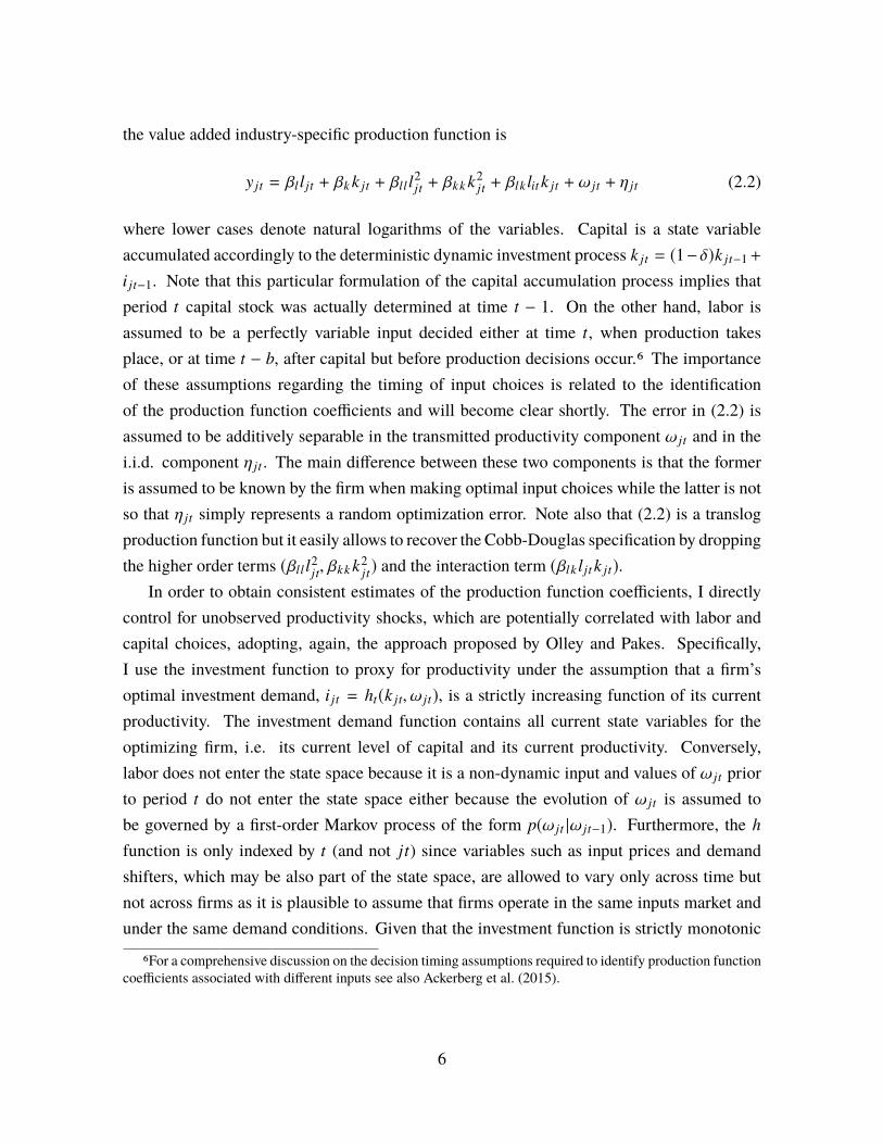
the value added industry-specific production function is

y jt = βl l jt + βk k jt + βll l2jt + βkk k2

jt + βlk lit k jt + ω jt + η jt (2.2)

where lower cases denote natural logarithms of the variables. Capital is a state variableaccumulated accordingly to the deterministic dynamic investment process k jt = (1−δ)k jt−1+

i jt−1. Note that this particular formulation of the capital accumulation process implies thatperiod t capital stock was actually determined at time t − 1. On the other hand, labor isassumed to be a perfectly variable input decided either at time t, when production takesplace, or at time t − b, after capital but before production decisions occur.6 The importanceof these assumptions regarding the timing of input choices is related to the identificationof the production function coefficients and will become clear shortly. The error in (2.2) isassumed to be additively separable in the transmitted productivity component ω jt and in thei.i.d. component η jt . The main difference between these two components is that the formeris assumed to be known by the firm when making optimal input choices while the latter is notso that η jt simply represents a random optimization error. Note also that (2.2) is a translogproduction function but it easily allows to recover the Cobb-Douglas specification by droppingthe higher order terms (βll l2

jt, βkk k2jt) and the interaction term (βlk l jt k jt).

In order to obtain consistent estimates of the production function coefficients, I directlycontrol for unobserved productivity shocks, which are potentially correlated with labor andcapital choices, adopting, again, the approach proposed by Olley and Pakes. Specifically,I use the investment function to proxy for productivity under the assumption that a firm’soptimal investment demand, i jt = ht(k jt, ω jt), is a strictly increasing function of its currentproductivity. The investment demand function contains all current state variables for theoptimizing firm, i.e. its current level of capital and its current productivity. Conversely,labor does not enter the state space because it is a non-dynamic input and values of ω jt priorto period t do not enter the state space either because the evolution of ω jt is assumed tobe governed by a first-order Markov process of the form p(ω jt |ω jt−1). Furthermore, the h

function is only indexed by t (and not jt) since variables such as input prices and demandshifters, which may be also part of the state space, are allowed to vary only across time butnot across firms as it is plausible to assume that firms operate in the same inputs market andunder the same demand conditions. Given that the investment function is strictly monotonic

6For a comprehensive discussion on the decision timing assumptions required to identify production functioncoefficients associated with different inputs see also Ackerberg et al. (2015).

6

in ω jt , it can be inverted to obtain

ω jt = h−1t (k jt, i jt) (2.3)

Following the same reasoning and maintaining the same assumptions on the evolution ofthe productivity process and the static/dynamic nature of the inputs, I also use the approachsuggested by Levinsohn and Petrin (2003). They observe that investment levels are, inmany cases, zero or very lumpy and propose to control for unobserved productivity using theintermediate input demand function as a proxy, instead. In this case, if the optimal expenditurelevel in intermediates, m jt = ft(k jt, ω jt), is assumed to be a strictly increasing function of thecurrent productivity, it can be inverted to generate

ω jt = f −1t (k jt,m jt) (2.4)

2.2.2 Estimation Procedure

Equations (2.3) and (2.4) show that investment or, alternatively, intermediate input demandcan be substituted into the production function as a proxy for the unobserved productivityterm ω jt , so that the estimating equation in (2.2) becomes

y jt = βl l jt + βk k jt + βll l2jt + βkk k2

jt + βlk l jt k jt + h−1t (k jt, i jt) + η jt (2.5)

or

y jt = βl l jt + βk k jt + βll l2jt + βkk k2

jt + βlk l jt k jt + f −1t (k jt,m jt) + η jt (2.6)

The estimation of (2.5) or (2.6) consists of two stages. The first stage serves the purposeof obtaining an estimate of the expected value added φ jt and an estimate of η jt alternativelyrunning the following regressions:

y jt = φt(l jt, k jt, i jt) + η jt (2.7)

or

y jt = φt(l jt, k jt,m jt) + η jt (2.8)

where in (2.7) φ jt = φt(l jt, k jt, i jt) = βl l jt + βk k jt + βll l2jt + βkk k2

jt + βlk l jt k jt + h−1t (k jt, i jt),

while in (2.8) φ jt = φt(l jt, k jt,m jt) = βl l jt + βk k jt + βll l2jt + βkk k2

jt + βlk l jt k jt + f −1t (k jt,m jt).

7

In addition, the functions h−1t in (2.5) and f −1

t in (2.6), are given by:

h−1t (k jt, i jt) = βk k jt + βii jt + βkk k2

jt + βiii2jt + βki k jti jt (2.9)

and

f −1t (k jt,m jt) = βk k jt + βmm jt + βkk k2

jt + βmmm2jt + βkmk jtm jt (2.10)

Note that, due to the specification of (2.9) and (2.10), in the first stage the coefficientsassociated with capital and capital squared in (2.5) and (2.6), respectively, are not identified.These coefficients will be identified only in the second stage of the estimation using anappropriate set of moment conditions. Moreover, under the Cobb-Douglas specification withthe investment demand or the intermediate inputs demand, i.e.

y jt = βl l jt + βk k jt + h−1t (k jt, i jt) + η jt (2.11)

or

y jt = βl l jt + βk k jt + f −1t (k jt,m jt) + η jt (2.12)

the coefficient associated with labor, βl , can be identified and estimated in the first stage aswell.

In the second stage, the (remaining) production function coefficients can be obtainedrelying on the Markov process assumption and the law of motion for productivity. Morespecifically, I model the productivity process non parametrically as a third degree polynomialof lagged productivity in the following way:

ω jt = γ0 + γ1ω jt−1 + γ2ω2jt−1 + γ3ω

3jt−1 + ξ jt (2.13)

Using the estimated φ jt from the first stage, the value of productivity for any given vector ofβ, where β = (βl, βk, βll, βkk, βlk), can be computed as:

ω jt(β) = φ jt − βl l jt − βk k jt − βll l2jt − βkk k2

jt − βlk l jt k jt (2.14)

By regressingω jt(β) on its lagω jt−1(β), it is possible to recover the innovation in productivitygiven by ξ jt(β). Specifically, denote βZ jt = βl l jt + βk k jt + βll l2

jt + βkk k2jt + βlk l jt k jt , then the

productivity process in (2.14) can simply be rewritten as ω jt(β) = φ jt − βZ jt and the term ξ jt

8

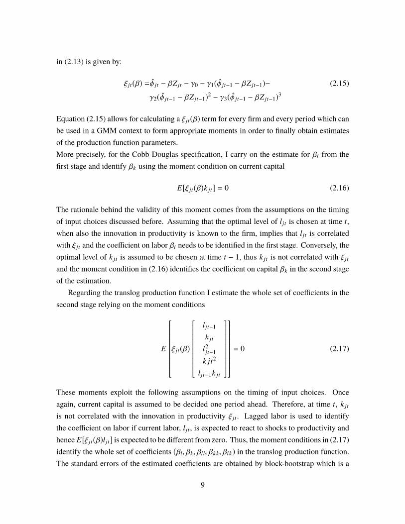
in (2.13) is given by:

ξ jt(β) =φ jt − βZ jt − γ0 − γ1(φ jt−1 − βZ jt−1)− (2.15)

γ2(φ jt−1 − βZ jt−1)2 − γ3(φ jt−1 − βZ jt−1)

3

Equation (2.15) allows for calculating a ξ jt(β) term for every firm and every period which canbe used in a GMM context to form appropriate moments in order to finally obtain estimatesof the production function parameters.More precisely, for the Cobb-Douglas specification, I carry on the estimate for βl from thefirst stage and identify βk using the moment condition on current capital

E[ξ jt(β)k jt] = 0 (2.16)

The rationale behind the validity of this moment comes from the assumptions on the timingof input choices discussed before. Assuming that the optimal level of l jt is chosen at time t,when also the innovation in productivity is known to the firm, implies that l jt is correlatedwith ξ jt and the coefficient on labor βl needs to be identified in the first stage. Conversely, theoptimal level of k jt is assumed to be chosen at time t − 1, thus k jt is not correlated with ξ jt

and the moment condition in (2.16) identifies the coefficient on capital βk in the second stageof the estimation.

Regarding the translog production function I estimate the whole set of coefficients in thesecond stage relying on the moment conditions

E

ξ jt(β)

l jt−1

k jt

l2jt−1

k jt2

l jt−1k jt

= 0 (2.17)

These moments exploit the following assumptions on the timing of input choices. Onceagain, current capital is assumed to be decided one period ahead. Therefore, at time t, k jt

is not correlated with the innovation in productivity ξ jt . Lagged labor is used to identifythe coefficient on labor if current labor, l jt , is expected to react to shocks to productivity andhence E[ξ jt(β)l jt] is expected to be different from zero. Thus, the moment conditions in (2.17)identify the whole set of coefficients (βl, βk, βll, βkk, βlk) in the translog production function.The standard errors of the estimated coefficients are obtained by block-bootstrap which is a

9

special bootstrap technique designed to maintain the structure of the panel.7 Specifically, Ibootstrap along the firm dimension, i.e. I randomly sample with replacement a number offirms equal to the number of firms present in each industry 400 times.

Two remarks regarding the estimation procedure are needed. First, I do not explicitlymodel entry and exit. This is because the panel I use is essentially closed given that, when afirm exited the sample, it was replaced by a similar firm and this new firm was assigned thesame identifier as the exiting one. Consequently, it is not possible to keep track of entry andexit patterns and focus on selection issues. However, as Griliches and Mairesse (1995) andLevinsohn and Petrin (2003) note, the selection correction seems tomake little difference oncethe simultaneity correction is in place. Second, I observe revenue instead of physical output,hence I actually estimate ’revenue’ production function parameters deflating the sales with anindustry-wide price index. This is an imperfect solution since, if the unobserved firm-specificoutput price index substantially differs from the industry price index, I am actually introducinga price error. Furthermore, if input decisions are correlated with the price error, the estimatedcoefficients of the production function may be biased downward because, as mentioned in theoriginal contribution by Klette and Griliches (1996), more inputs will lead to higher outputand decrease prices, ceteris paribus. Nonetheless, this imperfect solution appears to be thebest possible solution, given the limitations in the available data

2.3 A Structural Approach to Derive Firm-level Markups

My second empirical goal is to derive markup estimates at the firm-level. To achieve thisgoal I follow the approach proposed by De Loecker and Warzynski (2012), which has theadvantage of not depending on the availability of very detailed data. The data requirements,indeed, are limited to total expenditure on variable inputs (labor and materials), capital,investment and output at the firm-level. This approach is fairly direct from an economictheory perspective, since it relies on standard optimal input demand conditions that can beobtained from standard cost minimization. Moreover, it is straightforward to implementempirically, since the estimation is simply based on the insight that the cost share of factorsof production are not equal to their output revenue share when markets are not perfectlycompetitive, so that the estimated markups can be interpreted as a measure of market power.Finally, this approach is flexible as it can be applied to a wide range of production functionsand it is able to correct the markup bias by directly controlling for the firm-specific unobservedproductivity.

7For more details about the block-bootstrap technique see Horowitz (2001).

10

To derive an expression for markups consider, once again, a firm j in industry i at timet (the industry subscript is again omitted for simplicity) producing output Q jt using variableinputs (X1

jt, . . . , XVjt), which may include labor, materials, and energy, and capital K jt as

factors of production, and with productivity level ω jt . This firm aims to minimize its cost ofproduction by solving the problem

minXjt,Kjt

V∑v=1

PXv

jt Xvjt + r jtK jt (2.18)

s.t. Q jt = Q jt(X1jt, . . . , XV

jt,K jt, ω jt)

where PXv

jt denotes the price of any variable input and r jt denotes the price of capital. Thetechnology constraint takes a very general form and the only restriction imposed on Q jt(·) isthat it is continuous and twice differentiable with respect to its arguments. The Lagrangianassociated with the minimization problem in (2.18) is given by:

L(X jt,K jt, λ jt) =

V∑v=1

PXv

jt Xvjt + r jtK jt + λ jt(Q jt −Q jt(·)) (2.19)

with the first order condition with respect to each variable input being

∂L

∂Xvjt= PXv

jt − λ jt∂Q jt(·)

∂Xvjt= 0 (2.20)

where λ jt is the marginal cost of production.8Rearranging terms, multiplying both sides of (2.20) by X jt/Q jt , and dividing by λ jt yields

∂Q jt(·)

∂Xvjt

Xvjt

Q jt=

1λ jt

PXv

jt Xvjt

Q jt(2.21)

(2.21) simply states that cost minimization requires the optimal input demand being satisfied

when a firm equalizes the output elasticity of input Xvjt to

1λjt

PXv

jt Xvjt

Q jt.9

8The Lagrange multiplier λjt , in this context, measures the marginal cost of production since ∂L∂Q j t

= λjt .Formally, λjt represents the shadow value of the constraint, i.e. the increase in cost generated by a marginalexpansion in output.

9Note that, 1λ j t

PXv

jt Xvj t

Q j tis not input Xv

jt ’s cost share because, in general, λjtQ jt is not equal to the total costof production. Only in the special case of constant marginal cost, given the interpretation of the Lagrangemultiplier, (2.21) implies that, at the optimum, a firm equalizes the output elasticity of any variable input to its

11

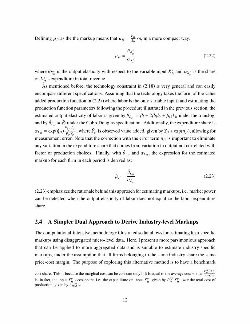
Defining µ jt as the the markup means that µ jt =Pjt

λjtor, in a more compact way,

µ jt =θXv

jt

αXvjt

(2.22)

where θXvjtis the output elasticity with respect to the variable input Xv

jt and αXvjtis the share

of Xvjt’s expenditure in total revenue.As mentioned before, the technology constraint in (2.18) is very general and can easily

encompass different specifications. Assuming that the technology takes the form of the valueadded production function in (2.2) (where labor is the only variable input) and estimating theproduction function parameters following the procedure illustrated in the previous section, theestimated output elasticity of labor is given by θLjt = βl + 2βll lit + βlk kit under the translog,and by θLjt = βl under the Cobb-Douglas specification. Additionally, the expenditure share is

αLjt = exp(η jt)PLjt

Ljt

PjtYjt, where Yjt is observed value added, given by Yjt + exp(η jt), allowing for

measurement error. Note that the correction with the error term η jt is important to eliminateany variation in the expenditure share that comes from variation in output not correlated withfactor of production choices. Finally, with θLjt and αLjt , the expression for the estimatedmarkup for each firm in each period is derived as:

µ jt =θLjt

αLjt

(2.23)

(2.23) emphasizes the rationale behind this approach for estimatingmarkups, i.e. market powercan be detected when the output elasticity of labor does not equalize the labor expenditureshare.

2.4 A Simpler Dual Approach to Derive Industry-level Markups

The computational-intensive methodology illustrated so far allows for estimating firm-specificmarkups using disaggregated micro-level data. Here, I present a more parsimonious approachthat can be applied to more aggregated data and is suitable to estimate industry-specificmarkups, under the assumption that all firms belonging to the same industry share the sameprice-cost margin. The purpose of exploring this alternative method is to have a benchmark

cost share. This is because the marginal cost can be constant only if it is equal to the average cost so thatPXv

jt Xvj t

λ j tQ j t

is, in fact, the input Xvjt ’s cost share, i.e. the expenditure on input Xv

jt , given by PXv

jt Xvjt , over the total cost of

production, given by λjtQ jt .

12

for comparison between a simpler and less demanding (in terms of data requirements andcomputational burden) approach and a more structural and onerous one.

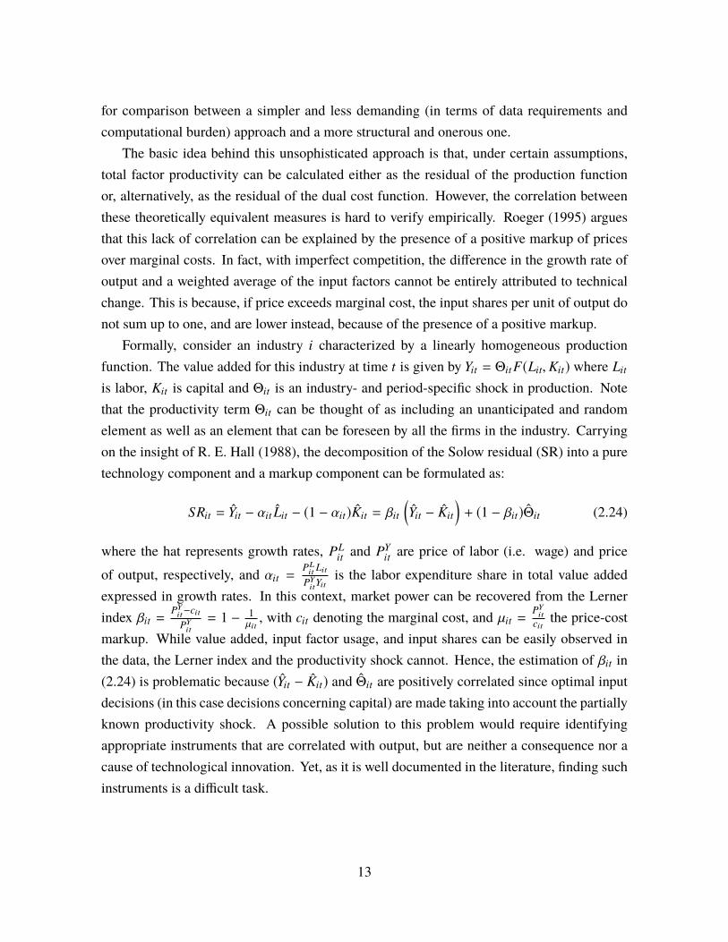
The basic idea behind this unsophisticated approach is that, under certain assumptions,total factor productivity can be calculated either as the residual of the production functionor, alternatively, as the residual of the dual cost function. However, the correlation betweenthese theoretically equivalent measures is hard to verify empirically. Roeger (1995) arguesthat this lack of correlation can be explained by the presence of a positive markup of pricesover marginal costs. In fact, with imperfect competition, the difference in the growth rate ofoutput and a weighted average of the input factors cannot be entirely attributed to technicalchange. This is because, if price exceeds marginal cost, the input shares per unit of output donot sum up to one, and are lower instead, because of the presence of a positive markup.

Formally, consider an industry i characterized by a linearly homogeneous productionfunction. The value added for this industry at time t is given by Yit = Θit F(Lit,Kit) where Lit

is labor, Kit is capital and Θit is an industry- and period-specific shock in production. Notethat the productivity term Θit can be thought of as including an unanticipated and randomelement as well as an element that can be foreseen by all the firms in the industry. Carryingon the insight of R. E. Hall (1988), the decomposition of the Solow residual (SR) into a puretechnology component and a markup component can be formulated as:

SRit = Yit − αit Lit − (1 − αit)Kit = βit

(Yit − Kit

)+ (1 − βit)Θit (2.24)

where the hat represents growth rates, PLit and PY

it are price of labor (i.e. wage) and priceof output, respectively, and αit =

PLit Lit

PYitYit

is the labor expenditure share in total value addedexpressed in growth rates. In this context, market power can be recovered from the Lernerindex βit =

PYit−citPYit

= 1 − 1µit, with cit denoting the marginal cost, and µit =

PYit

citthe price-cost

markup. While value added, input factor usage, and input shares can be easily observed inthe data, the Lerner index and the productivity shock cannot. Hence, the estimation of βit in(2.24) is problematic because (Yit − Kit) and Θit are positively correlated since optimal inputdecisions (in this case decisions concerning capital) are made taking into account the partiallyknown productivity shock. A possible solution to this problem would require identifyingappropriate instruments that are correlated with output, but are neither a consequence nor acause of technological innovation. Yet, as it is well documented in the literature, finding suchinstruments is a difficult task.

13

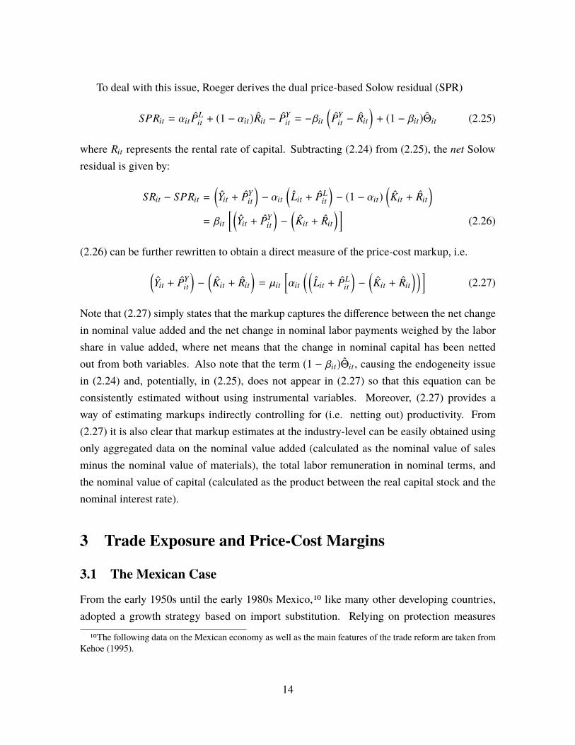
To deal with this issue, Roeger derives the dual price-based Solow residual (SPR)

SPRit = αit PLit + (1 − αit)Rit − PY

it = −βit

(PY

it − Rit

)+ (1 − βit)Θit (2.25)

where Rit represents the rental rate of capital. Subtracting (2.24) from (2.25), the net Solowresidual is given by:

SRit − SPRit =(Yit + PY

it

)− αit

(Lit + PL

it

)− (1 − αit)

(Kit + Rit

)= βit

[(Yit + PY

it

)−

(Kit + Rit

)](2.26)

(2.26) can be further rewritten to obtain a direct measure of the price-cost markup, i.e.(Yit + PY

it

)−

(Kit + Rit

)= µit

[αit

((Lit + PL

it

)−

(Kit + Rit

))](2.27)

Note that (2.27) simply states that the markup captures the difference between the net changein nominal value added and the net change in nominal labor payments weighed by the laborshare in value added, where net means that the change in nominal capital has been nettedout from both variables. Also note that the term (1 − βit)Θit , causing the endogeneity issuein (2.24) and, potentially, in (2.25), does not appear in (2.27) so that this equation can beconsistently estimated without using instrumental variables. Moreover, (2.27) provides away of estimating markups indirectly controlling for (i.e. netting out) productivity. From(2.27) it is also clear that markup estimates at the industry-level can be easily obtained usingonly aggregated data on the nominal value added (calculated as the nominal value of salesminus the nominal value of materials), the total labor remuneration in nominal terms, andthe nominal value of capital (calculated as the product between the real capital stock and thenominal interest rate).

3 Trade Exposure and Price-Cost Margins

3.1 The Mexican Case

From the early 1950s until the early 1980s Mexico,10 like many other developing countries,adopted a growth strategy based on import substitution. Relying on protection measures

10The following data on the Mexican economy as well as the main features of the trade reform are taken fromKehoe (1995).

14

against world competition and on government intervention in the domestic economy, thisstrategy encouraged investment in industry, suppressed agricultural prices and expandedgovernment enterprises. Between 1960 and 1981 Mexico experienced an average increase ofreal GDP of 7 percent per year - even accounting for the high rate of population growth overthe that period, this translated into an average increase of GDP per capita of 4 percent peryear. During the 1970-1982 period, however, the import substitution policy began to be lesseffective as policies of deficit spending and monetary expansion financed by public sectorborrowing from international banks were implemented. As a result, Mexico experiencedrising inflation which, together with a fixed nominal exchange rate, led to substantial realexchange rate appreciation and growing current account deficit. Despite the substantialeconomic imbalances, the Mexican economy continued to expand on an average growth rateof real GDP of 6.2 percent over 1970-1982.

In 1982 the import substitution policy, and the Mexican economy with it, fell apart.Faced with a massive public debt owned by foreign banks, sharply rising international interestrates, and falling oil prices due to the worldwide recession, Mexico could not meet its debtobligations. The peso collapsed, the government nationalized banks and implemented strictexchange rate controls and the economy entered a deep recession. In late 1982, under newlyelected President Miguel de la Madrid Hurtado, Mexico embarked on its first steps on the longroad to recovery. During the 1983-85 period, with the financial support of the InternationalMonetary Fund, the new administration implemented a series of policies designed to cut thepublic sector deficit and turn the large trade deficit into a surplus. These policies includedreduction in government expenditures, increases in taxes and in the prices of public services,elimination of many subsidies and closure of some public enterprises, enforcement of licenserequirements for all imports, and the abolition of the exchange rate controls. Although thisprogram was successful in creating a trade surplus and in partially lowering inflation, it wasnot enough to prevent another crisis. In late 1985 fiscal discipline began towaver, IMF fundingended, an earthquake in Mexico City caused disruption and imposed significant costs, and theoil prices started on a steep decline that continued until 1987.

The 1985-87 period was characterized by falling output and accelerating inflation. Itwas during this period, however, that Mexico began some of the policy reforms that werecrucial in bringing deficit and inflation rate to acceptable levels and restoring economicprosperity during the 1987-93 period. Major initiatives included privatization of state-ownedcompanies, deregulation of financial markets, liberalization of foreign investment, and adramatic re-orientation of trade policy.

The trade policy reforms were perhaps the most striking. In 1985 the process of apertura,

15

openness to foreign trade and investment, began and between 1982 and 1994 Mexico wentfrom being a relatively closed economy, even for developing countries’ standards, to beingone of the most open in the world. In 1982 tariffs were as high as 100 percent and there wassubstantial dispersion in tariff rates. Licenses were required for importing any good and, asa general rule, foreigners were restricted to no more than 49 percent ownership of Mexicanenterprises. In 1982 import licenses, not tariffs, wereMexico’s most significant trade barriers.Starting in late 1983 quantitative restrictions were replaced with tariffs. The portion of tariffitems subject to license requirements fell from 100 percent in 1983 to 65 percent in 1984and reached 10 percent in 1985. By 1992 it was just 2 percent. Even so, the portion ofthe value of imports subject to license requirements fell more slowly: from 100 percent in1983 to 83 percent in 1984, to 35 percent in 1985, to 11 percent in 1992. As import licenseswere replaced by tariffs as the major tool of trade policy, average tariffs initially rose andthen fell. The average tariff went from 23.2 percent in 1983 to 25.4 percent in 1985, to 13.1in 1992. The trade-weighed average tariff went from 8.0 percent in 1983 to 13.3 percentin 1985, to 11.1 percent in 1992. Equally effective with the change in average tariff rateswas the simplification of the tariff schedule. These measures were major steps in makingthe Mexican trade policy less protective and more transparent. They were accompanied bya number of other supporting policies: in 1986 Mexico acceded the GATT, adopting theHarmonized Commodity Description and Coding System, the Foreign Trade Law and theGATT Anti-Dumping Code. In short, in about five years Mexico dramatically liberalized itstrade regime. The liberalization process was almost complete by the end of 1987, althoughthe impact on the flow of imports was softened by real devaluations. The reforms helped topromote exports. In terms of both import penetration and export rates, the manufacturingsector became substantially open as a consequence.

3.2 Relating Markups and Measures of Trade Liberalization

Prior to the liberalization that begun in 1983, trade accounted for a small share of manufactur-ing production in most Mexican industries. Both the ratio of imports over domestic consump-tion and the ratio of exports over domestic production were below 10 percent. Nonetheless, asa consequence of the rapid and dramatic process of foreign trade and investment liberalization,in merely a decade Mexico became one of the most open economies in the world. In order toinvestigate whether this outward-looking reform generated import discipline —a decreasedin profitability, measured through markups, due to the removal of trade protections— I relyon two simple models that allow for quantifying the impact of trade liberalization on the

16

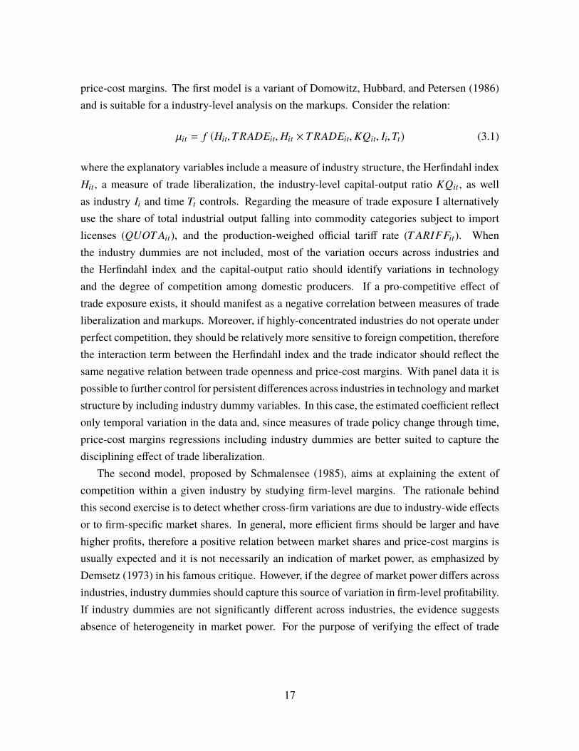
price-cost margins. The first model is a variant of Domowitz, Hubbard, and Petersen (1986)and is suitable for a industry-level analysis on the markups. Consider the relation:

µit = f (Hit,T RADEit,Hit × T RADEit,KQit, Ii,Tt) (3.1)

where the explanatory variables include a measure of industry structure, the Herfindahl indexHit , a measure of trade liberalization, the industry-level capital-output ratio KQit , as wellas industry Ii and time Tt controls. Regarding the measure of trade exposure I alternativelyuse the share of total industrial output falling into commodity categories subject to importlicenses (QUOT Ait), and the production-weighed official tariff rate (T ARIFFit). Whenthe industry dummies are not included, most of the variation occurs across industries andthe Herfindahl index and the capital-output ratio should identify variations in technologyand the degree of competition among domestic producers. If a pro-competitive effect oftrade exposure exists, it should manifest as a negative correlation between measures of tradeliberalization and markups. Moreover, if highly-concentrated industries do not operate underperfect competition, they should be relatively more sensitive to foreign competition, thereforethe interaction term between the Herfindahl index and the trade indicator should reflect thesame negative relation between trade openness and price-cost margins. With panel data it ispossible to further control for persistent differences across industries in technology andmarketstructure by including industry dummy variables. In this case, the estimated coefficient reflectonly temporal variation in the data and, since measures of trade policy change through time,price-cost margins regressions including industry dummies are better suited to capture thedisciplining effect of trade liberalization.

The second model, proposed by Schmalensee (1985), aims at explaining the extent ofcompetition within a given industry by studying firm-level margins. The rationale behindthis second exercise is to detect whether cross-firm variations are due to industry-wide effectsor to firm-specific market shares. In general, more efficient firms should be larger and havehigher profits, therefore a positive relation between market shares and price-cost margins isusually expected and it is not necessarily an indication of market power, as emphasized byDemsetz (1973) in his famous critique. However, if the degree of market power differs acrossindustries, industry dummies should capture this source of variation in firm-level profitability.If industry dummies are not significantly different across industries, the evidence suggestsabsence of heterogeneity in market power. For the purpose of verifying the effect of trade

17

liberalization on profitability at the firm level consider the following specification:

µ jit = f(Sjit, S2

jit,T RADEit, Sjit × T RADEit,KQ jit,KQ2jit, Ii,Tt

)(3.2)

where the price-cost margin µ jit of firm j in industry i in year t depends on its share of outputin total domestic manufacturing production, Sjit and S2

jit , on the capital-output ratio KQ jit ,on an industry-specific measure of trade exposure, T RADEit , as well as industry and yeardummy variables.

3.3 Relating Markups and Export Status

The two previous models relate markups with trade exposure using trade indicators thatmainly capture the extent of import liberalization. In fact, both the quota coverage and theaverage tariff rate measure protective restrictions on imports. A number of recent modelsof international trade, however, emphasize the implications of trade openness, productivityand profitability for exporters. More specifically, these models generate the result that moreproductive firms are more profitable because they can charge higher markups. The higherprofitability allows these firms to pay an export entry cost and become exporters, thus exportershave usually higher markups. In the literature two main reasons for this positive relationbetween markups and firm’s export status have been identified. Bernard et al. (2003), as wellas Melitz and Ottaviano (2008) attribute the source of the markup premium for exportersto differences in productivity. Both contributions essentially predict that exporters willcharge higher markups because they are more productive than their domestic rivals and thisproductivity wedge allows them to be more profitable and more competitive.11 On the otherhand, Kugler and Verhoogen (2011) and Hallak and Sivadasan (2013) explore the role ofquality differences between exporters and non exporters assuming that, if exporters produce

11It is important to note that not all the recent models of international trade imply that exporters, whoare assumed to be more productive than non-exporters, are more profitable because they are able to chargehigher markups. For example, with an isoelastic demand system, like the CES demand system in Melitz(2003), exporters are more productive and more profitable but do not charge higher markups. Their additionalprofitability comes from the fact that higher levels of productivity allow them to have lower marginal costs sothat the point where the marginal revenue equalizes the marginal cost is further down the demand schedulegranting them more sales. Conversely, exporters are able to charge higher markups in Melitz and Ottaviano(2008)’s model because the demand system is linear with horizontal product differentiation and markups areendogenous and depend on the size of a market and the extent of its integration through trade. In Bernardet al. (2003)’s model imperfect competition is the mechanism leading to variable markups. Specifically, withBertrand competition producers who are more efficient tend to have a greater cost advantage over their closestcompetitors, set higher markups and appear more productive. More efficient producers are more likely to beatrivals in foreign markets and this is the reason why exporters tend to be more productive than non-exporters.

18

higher quality goods while using higher quality inputs, they can charge higher markups, allother things equal.

Given that with the structural approach I can estimate firm-level markups, I can easilyrelate a firm’s markup to its export status in a regression framework as follows:

ln(µ jt) = ψ0 + ψ1E jt + z jtρ + ε jt (3.3)

where µ jt is the markup for firm j at time t and E jt is a dummy variable that takes the valueof one when firm j is an exporter. Thus, the coefficient associated with this dummy, ψ1,measures the percentage markup premium for exporters. In addition, z jt is a set of variablesincluding capital and labor use that control for differences in size and factor intensity, as wellas year- and industry-specific dummy variables that control for aggregate trends in markups.The vector ρ collects the coefficients associated with the whole set of controls. After obtainingan estimate for ψ1, it is possible to recover the level markup difference, denoted as µE , bycalculating the percentage difference with respect to the constant term ψ0, which captures themarkup average for domestic firms. Specifically, µE = ψ1 exp(ψ0). A positive and significantµE would imply that there is in fact a markup premium for exporters with respect to domesticproducers.

4 Data

My entire analysis is conducted using plant-level panel data collected through Mexico’sAnnual Industrial Survey by the Mexican statistical agency INEGI. These data were madeavailable by Mexico’s Secretariat of Commerce and Industrial Development (SECOFI), (nowSecretariat of Economy) and includes a sample of activeMexicanmanufacturing plants duringthe period 1984-1990.12

For a typical industry, the sample is representative of about 80 percent of the total output inthat industry therefore, even if the smallest plants were excluded, the sample can be consideredfairly representative. Note that, because of the way the data are reported, it is not possible to

12Note that the analysis has been conducted for the period 1984-1990 and cannot be extended in an immediateand straightforward way to more recent years for the following reasons. First, accessing more recent productiondata would now require being granted access to the Laboratorio de Microdatos at INEGI. Second, the productionand trade data used in this paper were specifically matched to obtain measures of trade liberalization at the firmlevel based on the import/export composition of each firm. This level of accuracy and precision in the matchingis not easily replicable given that disaggregated production and trade data are currently housed in different places(INEGI and Banco de México, respectively) and cannot be merged for confidentiality reasons.

19

identify which plants belong to the same firm. Therefore, even if there are certainly multi-plant firms in the sample, I formally treat a plant as a firm and do not try to capture theextent to which multi-plant firms may have a different strategic production behavior due totheir multi-plant nature. For this reason the words firm and plant are used interchangeably,as it is not possible to make a meaningful distinction between these concepts in my data.Furthermore, as mentioned before, when a firm exited the sample, it was replaced with a firmwith similar production characteristics and the new firm was assigned the same identifier asthe exiting one. Thus, the panel can be considered essentially closed as it is not possible tokeep track of entry and exit patterns. The panel is however unbalanced since a (marginally)decreasing number of firms is included in the sample over the years.

For each plant in each year it is possible to observe data on value of production, revenue,input expenditure, labor remunerations, value of fixed capital, investment, inventories, andinput costs. Each plant can be traced and uniquely identified over time using a combination ofindustry (RAMA), class (CLASE) and plant (FOLIO) identity codes. The dataset also containsprice indices at the industry level for output and intermediate inputs, as well as sector-widedeflators for machinery and equipment, buildings and land. Moreover, the dataset containsdetailed information about imports, exports, and commercial policy features like coverage ofimport license and tariff rates at the industry level. This information is particularly useful todescribe the Mexican trade liberalization process and to verify its effects on the price-costmargins.

4.1 DataPreparation: RelevantVariables andSample SelectionCriteria

The original sample consisted of 22,526 observations on 3,218 plants during the period 1984-1990. All the variables used in the analysis are reported in table 1, the monetary variableswere converted to millions of 1980 Mexican pesos using specific deflators.

In addition, I use some of the original variables present in the dataset to construct newvariables useful for the analysis. These variables, their description and the calculation detailsare reported in table 2. First, the expenditure in intermediates was calculated without takinginto account inventories. This choice was dictated by the fact that in 1985 the variablescharacterizing inventories presented many missing observations thus, following one of thesample selection criteria (described in detail below) of withdrawing incomplete series, toconsider inventories would have caused the elimination of half of the plants from the analysis.Second, total capital stock for each plant was calculated as the sum of replacement costof capital and the capitalized value of the rents with a 10 percent discount rate. Third,

20

the variables involved in the calculation of the value added and the value added itself werecorrected in order to account for the measurement error in the intermediate inputs expenditurefor the maquiladoras.13 Specifically, the value added was corrected adding the income fromsubcontracting and subtracting the cost of subcontractors. The gross value of output, whichsuffers from the same bias, was corrected under the assumption that the ratio between valueadded and output and between primary materials and total inputs are constant through timeand among plants running the following regression:14 CORGVO = GVO + b( INSE RM AQ

PM −GAST M AQU

PM ). The value of the b15 parameter used in the correction was estimated at a two-digit national accounts classification level (RAMA) using only the plants that did not conductmaquila activities. Finally, the corrected value of expenditure in intermediates was simplycalculated by subtracting the corrected value added from the corrected value of gross output.

Around 20 percent of the original observations were eliminated discarding those that forat least one year had negative, zero, and missing values of the following variables: totalemployment, total hours worked, capital stock, gross value of output, corrected gross value ofoutput, value added, corrected value added, intermediates, corrected intermediates, and laborremunerations. This process resulted in the elimination of 4,234 observations. Among theremaining 18,292 observations, additional 4,924 observations were eliminated dropping theincomplete series. That is, all the observations pertaining to plants that were discarded for atleast one year because of one or more of the above reasons were completely eliminated fromthe sample in order to include only plants for which complete information for all the yearswas available. The final sample used in the analysis contained 13,368 observations on 2,088plants. Moreover, in order to carry on the structural production function estimation usingthe investment as a proxy for productivity, 2,092 observations were further dropped in orderto create the investment series. Finally, two sectors, Tobacco and Nonferrous metals, weredropped because the extremely low number of plants left after the sample selection was notadequate to perform a meaningful empirical analysis in those two industries.

13Themaquiladora is a firm-concept very common inMexico. Maquiladoras are manufacturing firms that areallowed to import materials and equipment on a duty-free and tariff-free basis for assembling or manufacturingand then either sell the assembled or manufactured products to the domestic firm which commissioned themaquila service or re-export the products outside the Mexican border. Themaquiladoras generate measurementerror because the Mexican accounting system attributes to the firm that order the subcontracting service theexpenditure in intermediates actually used by the subcontractor.

14See table 2 for a detailed description of the variables involved in this regression.15The average value of b is 1.47 with standard deviation 0.12.

21

4.2 Sample Characteristics

Table 3 reports in detail the industrial classification codes aggregated into each sector, theaverage number of plants in each sector, as well as some other characteristics that describethe relative importance of each sector in the total manufacturing output and the openness totrade. As shown in table 3 there is substantial heterogeneity in all these characteristics amongthe Mexican manufacturing industries considered in the analysis.

Table 4 summarizes the data by presenting the number of plants and various indicatorsof plant size pooling all the manufacturing plants during the period 1985-1990. Exceptfor 1986, average plant growth is positive whether measured by gross output, value added,or total employment and it is particularly high in the last 2 years included in the sample.Average capital stock per plant decreases from 1985 to 1986, probably as a consequence ofthe physical destruction caused by the earthquake of 1985 and the low level of net investmentduring the recession of 1986. Its upward trend after 1987 is consistent with the recovery ofthe economy and the exit from the sample of small firms, which occurs mainly in 1989-1990.Capital productivity is characterized by ups and downs during the entire period and this mayreflect underutilization of capacity and delays in replacing old equipment. Finally, investmentfollows also a very irregular pattern with sharp drops in 1986 and 1988 which are also likelypicking up the adverse effects of the earthquake and the recession. Additional variables thatare used in the regression models and further help to characterize the Mexican manufacturingenvironment are reported in table 6.

4.3 Trade Statistics

The trade data on imports and exports, used to calculate the statistics at the industry levelreported in the last three columns of table 3, came from the Commodity Trade databaseof the United Nations Statistical Office, which provides information at the four-digit levelISIC classification and categorizes products by end of use. These data were merged withthe Mexico’s Annual Industrial Survey, which, on the other hand, categorizes products byproduction technology, trying to achieve a reasonable match relying on detailed product codesavailable in the industrial survey. Also, since the trade data are reported in US dollars, theywere first converted into 1980US dollars and then intoMexican pesos using the 1980 exchangerate in order to render the figures comparable removing the exchange rate fluctuations.

In addition, the data on commercial policies were provided by the SECOFI and werealready harmonized with the classification scheme of the industrial census. These data,

22

summarized by industry and time sub-periods in table 5, clearly demonstrate that most of thechanges in commercial policy took place between 1985 and 1988.

5 Production Function Estimation Results

In this section I exploit the structural framework described in section 2.2 to estimate pro-duction function parameters controlling for endogenous productivity for eighteen Mexicanmanufacturing sectors. I estimate several models under different production technology spec-ifications (Cobb-Douglas and translog) with both the Olley and Pakes and Levinson andPetrin approaches. The estimation results suggest that the Cobb-Douglas specification withthe investment function used as a proxy for productivity (Olley and Pakes method) is themost adequate to fit the data, therefore I provide all the main results on production functionparameters and productivity adopting this specification. At the end of the section I report andcomment on robustness check results obtained with alternative models.

5.1 Production Function Parameters

I begin by presenting the production function estimates for the whole sample comparing thestructural estimation results with the ones obtained using more standard OLS and fixed effectsestimation techniques. I then test whether there is statistically significant evidence that theproduction function coefficients change during the period considered.

5.1.1 Comparing Different Estimators

The last two columns of table 7 report the results obtained estimating a Cobb-Douglas pro-duction function using the investment as a proxy for productivity (Olley and Pakes approach).Specifically, in the first stage equation (2.11) is estimated with OLS. The results of the firststage estimation, i.e. φ jt and η jt , are carried through the second stage where the residual ξ jt

of the productivity process from equation (2.13) is again obtained by OLS. Finally, equation(2.15) is estimated by GMM exploiting the moment condition on capital in (2.16). Note that,since the coefficient on labor βl is identified and estimated in the first stage, I rely on onemoment condition to identify the only remaining parameter, βk , in the second stage. Thus,the system is just identified and the identity matrix is the optimal weighting matrix used inthe GMM objective function.In almost all sectors, with the exception of Food (1) and Glass (11), the coefficient associated

23

with labor is significant and ranges from 0.15 in Chemicals (9) to 0.96 in Leather and Footwear(6). The coefficient on capital, on the other hand, is significant for only twelve out of eighteensectors and ranges from 0.36 in Plastic and Rubber (10) to 0.74 in Nonelectrical machinery(17). As expected, there are significant differences in the production function parameters,thus in technology, across sectors. In particular, some sectors like Clothing and Apparel (5),and Plastic and Rubber (10) are more labor intensive, while other sectors like Pulp and Paper(8), Chemicals (9), and Transportation equipment (19) are more capital intensive.

The comparison between the results from the structural estimations and those obtainedwitha simple OLS regression yields a well established empirical evidence. First, the coefficients onlabor and capital are highly statistically significant across all sectors. Second, focusing only onthe coefficients that are significant in the structural estimation, the OLS coefficient on labor isalways larger while the coefficient on capital is always smaller than its structural counterpart.This pattern is well documented in the literature and is determined by the correlation structurebetween the transmitted productivity shock and the production inputs. More precisely, thevariable input labor is supposed to be positively correlated with the unobserved productivity,thus the OLS coefficient on labor is likely to be biased upward. On the other hand, if currentcapital is not correlated with the current productivity shock, as it is decided one period ahead,or if capital is much less correlated with productivity than labor, the OLS estimate on capitalis likely to be biased downward.

Finally, looking at the estimates obtained using plant-level fixed effects (third and fourthcolumn of table 7), it is clear that, at least for labor, this approach partially mitigates the biasdiscussed above, i.e. the fixed effect coefficient on labor is always significant and smaller thanthe OLS one. However, the estimation of the capital parameter under fixed effects appearsmore problematic with some insignificant values and an unclear pattern with respect to themagnitude of the coefficient, which is higher than its OLS counterpart in some cases butsmaller in some other cases. Nonetheless, the fixed effects estimates still remain higher forlabor and lower for capital than those obtained with the structural approach. This is becausethe former is just an indirect way of controlling for unobserved productivity, whereas the latterfully and explicitly accounts for transitory productivity shocks.

With Cobb-Douglas technology, the production function coefficients represent the elas-ticity of output with respect to the inputs and their sum can be interpreted as returns to scale.Table 8 reports the estimated returns to scale, i.e. βl + βk . With OLS in most of the industriesthe sum of the two coefficients is very close to one but the constant returns to scale hypothesisis statistically verified only for half of the industries. The within estimator (plant-level fixedeffects) delivers returns to scale that are in general below one and overall lower than in the

24

OLS case. However, for fourteen industries constant returns to scale are statistically verified.Finally, the returns to scale estimated with the structural procedure are mostly in betweenthe OLS and FE results and, again, in thirteen out of eighteen industries the constant returnsto scale hypothesis cannot be rejected. Since the structural approach, and to some extentalso the FE, should deliver more credible estimates as they control (directly or indirectly) forproductivity shocks, the empirical evidence seems to support the presence of constant returnsto scale in the majority of the Mexican manufacturing industries.

5.1.2 Testing for a Structural Change in the Production Function Parameters

In order to verify whether the trade liberalization process generated factor reallocation phe-nomena across the Mexican manufacturing industries by modifying the factor intensity, Ire-estimate the structural model dividing the sample into two sub-periods, the first from 1985to 1987 and the second from 1988 to 1990. This choice is dictated by the fact that in thefirst three years (1985-1987) the most dramatic reforms took place, while the last three years(1988-1990) can be mainly considered a consolidation period. In order to carry out the test Imodify (2.11) and (2.13) in the following way:

y jt =βl l jt + βl Dt l jt + βk k jt + βk Dt k jt + βk k jt +˜βk Dt k jt + βii jt + βiDti jt

+ βkk k2jt + βkk Dt k2

jt + βiii2jt + βiiDti2

jt + βki k jti jt + βkiDt k jti jt + η jt (5.1)

ω jt =γ0 + γ0Dt + γ1ω jt−1 + γ2ω2jt−1 + γ3ω

3jt−1 + ξ jt (5.2)

where Dt is a dummy variable taking the value of one from 1988 on and zero otherwise. Notethat in (5.2) only the constant, i.e. the average productivity, is allowed to change between thetwo sub-periods. The intuition behind (5.1) is simply that there is evidence of a structuralchange in the production function parameters if βl and βk are significantly different from zero.

Table 9 shows that, reasonably, in almost all the cases the estimated coefficients for thetwo sub-periods can be considered as an upper and lower bound for the coefficients estimatedusing the whole sample (reported in the last two columns of table 7). However, the firsttwo columns of table 9 demonstrate that, especially for the capital coefficient, the divisionof the sample compromises the significance of the estimates. Moreover, regarding capital,the coefficient associated with the dummy variable is never significant meaning that thereis no evidence that the capital parameter changed in the second part of the sample. As forlabor, a significant structural change occurs after 1987 for just five industries: Beverages (2),Textiles (4), Chemicals (9), Plastic and Rubber (10), and Nonmetal minerals (13), with the

25

labor coefficient always increasing in the second sub-period. Nonetheless, since only in theChemicals industry the capital coefficient is significant in the first sub-period and does notchange between the two sub-periods, I conclude that, overall, the factor intensity remainedfairly constant during the trade liberalization process for the majority of the industries withthe exception of the Chemicals sector which became more labor-intensive. The coefficientassociated with the dummy variable in (5.2), not reported here, is insignificant in everyindustry suggesting that the average productivity did not change from the first sub-period tothe second.

5.2 Productivity Analysis

The structural framework illustrated in section 2.2 is suitable for obtaining a characterizationof the technology in each industry through the production function coefficients, as wellas an estimate of the productivity process for each firm in each year. Specifically, witha Cobb-Douglas technology, the productivity process can be recovered, after estimatingβl and βk , as ω jt = φ jt − βl l jt − βk k jt . Furthermore, recall that the first-order Markovproductivity process is modeled as a third degree polynomial of lagged productivity of theform: ω jt = γ0 + γ1ω jt−1 + γ2ω

2jt−1 + γ3ω

3jt−1 + ξ jt .

The empirical evidence suggests that, since for almost all the industries the γ0, γ2, andγ3 coefficients are statistically insignificant, the productivity process can be actually ap-proximated by the AR(1) process ω jt = γ1ω jt−1 + ξ jt . Therefore, the current productivitydepends only linearly on the value of the previous productivity. Moreover, the γ1 coefficientis estimated to be always below one (except for the Cement industry (12)) meaning that theproductivity process is stationary. Figure 1 depicts the productivity process for four industrieschosen for illustrative purposes.

For two of these four industries, figure 2 shows the smoothed plots for capital and in-vestment. Specifically, in each panel the vertical axis measures the estimated productivityshock, while the horizontal axis running left measures investment levels and the horizontalaxis running right measures capital usage. The structural estimation procedure is based on acrucial monotonicity assumption regarding productivity and investment, i.e. the investmentlevel should increase in productivity, conditioning on any observed levels of capital usage.As demonstrated in figure 2 this monotonicity condition appears to hold.

The ability of obtaining a direct estimate of the productivity process allows for analyzingthe growth in productivity for each firm from one year to the next. In fact, knowing ω jt , thegrowth in productivity can be easily calculated as ∆ω jt = ω jt − ω jt−1. Table 10 displays

26

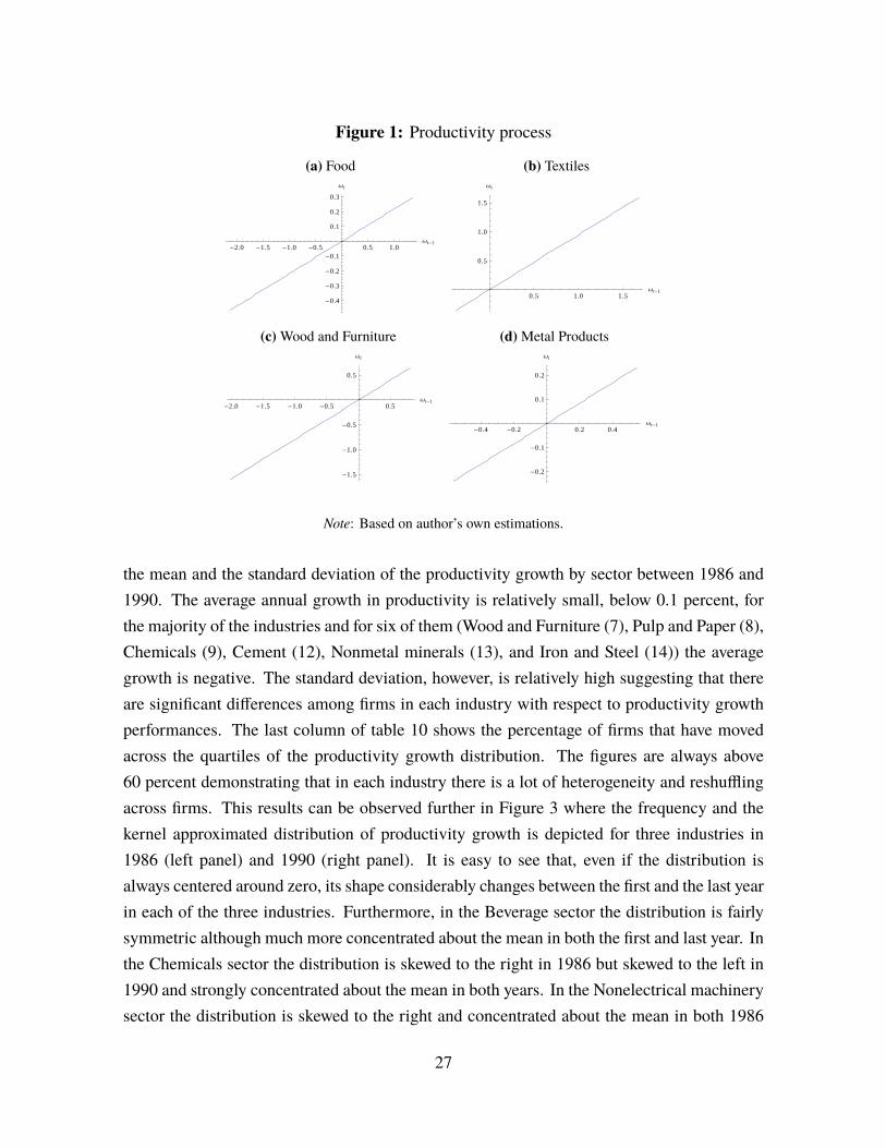
Figure 1: Productivity process

(a) Food

-2.0 -1.5 -1.0 -0.5 0.5 1.0

Ωt-1

-0.4

-0.3

-0.2

-0.1

0.1

0.2

0.3

Ωt

(b) Textiles

0.5 1.0 1.5

Ωt-1

0.5

1.0

1.5

Ωt

(c)Wood and Furniture

-2.0 -1.5 -1.0 -0.5 0.5

Ωt-1

-1.5

-1.0

-0.5

0.5

Ωt

(d) Metal Products

-0.4 -0.2 0.2 0.4

Ωt-1

-0.2

-0.1

0.1

0.2

Ωt

Note: Based on author’s own estimations.

the mean and the standard deviation of the productivity growth by sector between 1986 and1990. The average annual growth in productivity is relatively small, below 0.1 percent, forthe majority of the industries and for six of them (Wood and Furniture (7), Pulp and Paper (8),Chemicals (9), Cement (12), Nonmetal minerals (13), and Iron and Steel (14)) the averagegrowth is negative. The standard deviation, however, is relatively high suggesting that thereare significant differences among firms in each industry with respect to productivity growthperformances. The last column of table 10 shows the percentage of firms that have movedacross the quartiles of the productivity growth distribution. The figures are always above60 percent demonstrating that in each industry there is a lot of heterogeneity and reshufflingacross firms. This results can be observed further in Figure 3 where the frequency and thekernel approximated distribution of productivity growth is depicted for three industries in1986 (left panel) and 1990 (right panel). It is easy to see that, even if the distribution isalways centered around zero, its shape considerably changes between the first and the last yearin each of the three industries. Furthermore, in the Beverage sector the distribution is fairlysymmetric although much more concentrated about the mean in both the first and last year. Inthe Chemicals sector the distribution is skewed to the right in 1986 but skewed to the left in1990 and strongly concentrated about the mean in both years. In the Nonelectrical machinerysector the distribution is skewed to the right and concentrated about the mean in both 1986

27

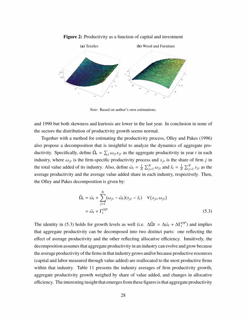
Figure 2: Productivity as a function of capital and investment

(a) Textiles

-5

0

i-4

-2

0

2

k

0.0

0.5

Ω

(b) Wood and Furniture

-8

-6

-4

-2

0

i

-4

-2

0

2

k

-2

-1

0

Ω

Note: Based on author’s own estimations.

and 1990 but both skewness and kurtosis are lower in the last year. In conclusion in none ofthe sectors the distribution of productivity growth seems normal.

Together with a method for estimating the productivity process, Olley and Pakes (1996)also propose a decomposition that is insightful to analyze the dynamics of aggregate pro-ductivity. Specifically, define Ωt =

∑j ω jt s jt as the aggregate productivity in year t in each

industry, where ω jt is the firm-specific productivity process and s jt is the share of firm j inthe total value added of its industry. Also, define ωt =

1N

∑Nj=1 ω jt and st =

1N

∑Nj=1 s jt as the

average productivity and the average value added share in each industry, respectively. Then,the Olley and Pakes decomposition is given by:

Ωt = ωt +

N∑j=1(ω jt − ωt)(s jt − st) ∀s jt, ω jt

= ωt + ΓOPt (5.3)

The identity in (5.3) holds for growth levels as well (i.e. ∆Ωt = ∆ωt + ∆ΓOPt ) and implies

that aggregate productivity can be decomposed into two distinct parts: one reflecting theeffect of average productivity and the other reflecting allocative efficiency. Intuitively, thedecomposition assumes that aggregate productivity in an industry can evolve and growbecausethe average productivity of the firms in that industry grows and/or because productive resources(capital and labor measured through value added) are reallocated to the most productive firmswithin that industry. Table 11 presents the industry averages of firm productivity growth,aggregate productivity growth weighed by share of value added, and changes in allocativeefficiency. The interesting insight that emerges from these figures is that aggregate productivity

28

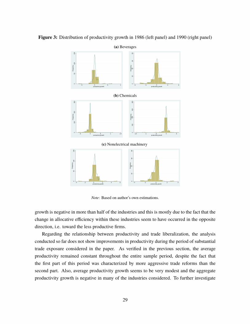
Figure 3: Distribution of productivity growth in 1986 (left panel) and 1990 (right panel)

(a) Beverages

050

100

150

Fre

quen

cy

-.5 0 .5 1productivity growth

020

4060

80F

requ

ency

-.4 -.2 0 .2 .4productivity growth

(b) Chemicals

010

020

030

0F

requ

ency

-.5 0 .5 1 1.5productivity growth

010

020

030

040

0F

requ

ency

-1.5 -1 -.5 0 .5productivity growth

(c) Nonelectrical machinery

050

100

150

Fre

quen

cy

-.4 -.2 0 .2 .4 .6productivity growth

020

4060

80F

requ

ency

-.4 -.2 0 .2 .4productivity growth

Note: Based on author’s own estimations.

growth is negative in more than half of the industries and this is mostly due to the fact that thechange in allocative efficiency within these industries seem to have occurred in the oppositedirection, i.e. toward the less productive firms.

Regarding the relationship between productivity and trade liberalization, the analysisconducted so far does not show improvements in productivity during the period of substantialtrade exposure considered in the paper. As verified in the previous section, the averageproductivity remained constant throughout the entire sample period, despite the fact thatthe first part of this period was characterized by more aggressive trade reforms than thesecond part. Also, average productivity growth seems to be very modest and the aggregateproductivity growth is negative in many of the industries considered. To further investigate

29

the relationship between trade openness and productivity gains,16 I calculate the Spearmanrank correlation coefficients between measures of productivity growth and measure of tradeliberalization displayed in table 12.17 Several patterns are worth noting. First, focusingon aggregate productivity growth is more appropriate than focusing on average productivitygrowth because aggregate productivity is a more insightful measure as it takes into accountthe share of each firm in the total value added of its industry. Second, changes in tradeopenness are negatively correlated with changes in aggregate productivity and allocativeefficiency, implying that an increase in trade openness (which corresponds to a decrease inquotas and tariffs) is associated with increases in both aggregate productivity and allocativeefficiency. This result seems to suggest that trade liberalization had a positive effect onthe productivity of the Mexican manufacturing firms. However, as the correlations betweenchanges in productivity and trade measures is significant but very small and the productivityanalysis conducted so far provided limited evidence of productivity gains, the positive effectis indeed quite modest.

5.3 Robustness Checks with Alternative Models

In this section I compare the production function coefficient estimates obtained applying thestructural approach to alternative models. In particular, I estimate the following additionalspecifications:

i. Value added with translog technology using the investment as a proxy for productivity(Olley and Pakes method) and estimating all the production function coefficients in thesecond stage relying on the moment conditions in (2.17).

ii. Value added with Cobb-Douglas technology using the demand for intermediate inputsas a proxy for productivity (Levinson and Petrin method), estimating the coefficient onlabor in the first stage and the coefficient on capital in the second stage relying on themoment condition in (2.16).

iii. Value added with translog technology including intermediate inputs in the produc-tion function (Levinson and Petrin method) and estimating all the production functioncoefficients in the second stage relying on the moment conditions in (2.17).

16See also Krishna and Mitra (1998) and Pavcnik (2002) for empirical contributions studying the effects oftrade liberalization on firm productivity in other developing countries.

17A similar table is presented in Tybout and Westbrook (1995) who use the same Mexican data utilized in thispaper to study changes in efficiency induced by the trade liberalization reform.

30

iv. Gross output with Cobb-Douglas technology including intermediate inputs in the pro-duction function (Levinson and Petrin method) and relying on the moment conditions oflagged labor, lagged intermediate inputs, and current capital to identify the coefficientsassociated with labor, intermediate inputs, and capital, respectively, in the second stage.

The results for the specifications ii. and iv. are omitted here because the estimation ofthese models was particularly problematic. The solving algorithm could not find a solutionsatisfying the optimization criteria and the resulting production function parameters were inmany cases zero, which implies that, since I imposed the restriction for the βs to be nonnega-tive, this constraint was often binding. The results for specifications i. and iii. are presented intables 13, 14, and 15, respectively. In particular, I estimate specification iii. twice, using theentire sample first and then using a subsample excluding the maquiladoras. This is becausethe Mexican accounting system includes in the books of the firm that orders a subcontractingservice the value of expenditure in intermediate inputs used by the subcontractor, generatinga measurement error problem with the intermediate inputs.

The results in tables 13, 14, and 15 demonstrate that, even if the translog specificationallows for amore flexible way ofmodeling technology, the overall significance of the estimatesis much lower because the higher order and interaction terms potentially generate collinearityissues. Moreover, the interpretation of the coefficients and returns to scale is complicatedwith translog production functions because the sign and the magnitudes of the coefficients donot have a straightforward meaning as they capture more elaborated and complex interactionsbetween inputs. The lack of significance is exacerbated when the intermediate inputs demandis used as a proxy for productivity, as confirmed by the results reported in tables 14 and 15. Thecause of this problem is likely to be themeasurement error in intermediate inputs, originated bythe peculiar way of recording expenditure in intermediates for themaquiladoras,18 which doesnot appear to be resolved even when these firms are excluded. In fact, a crucial requirementfor the Levinson and Petrin method to be successfully applied is the absence of measurementerror in intermediate inputs expenditure.

6 Price-Cost Margins Results

In this section I present the results on the industry-levelmarkups estimatedwith the simple dualapproach outlined in Section 2.4. I then compare these with the plant-level markups derived

18Theway of recording expenditure in intermediates for themaquiladoras affects both the production accountsof the maquiladoras and the firms that subcontract the maquila services.

31

by plugging into equation (2.23) the production function parameters previously obtainedwithin the structural framework. Finally, with the results of the markup estimations in hand,I investigate the relation between price-cost margins and trade openness.

6.1 Industry-level Markups

Table 16 reports the mean, median, and standard deviation of the year- and industry-specificmarkups recovered by estimating (2.27) by OLS. Note that with this procedure it is onlypossible to estimate one markup for each industry in each year, therefore the variation isalong the cross-sectional (industry) dimension. The average markup ranges between 0.24for Chemicals (9) and 2.69 for Cement (12) and in almost all the industries the mean andthe median are different, with the mean being usually higher than the median, implyingthat the distribution of the markups is not symmetric. Moreover, the standard deviation ishigh indicating that in every industry the markups vary consistently across years. In manyindustries the magnitude of the markups is quite unreasonable (significantly lower than one)and the significance of the estimates is fairly poor. Overall this simple estimation proceduredelivers very imprecise and unreliable results and it does not appear to be a valid alternativeto the structural approach.

6.2 Plant-level Markups

Table 17 summarizes the plant-level markups recovered combining the output elasticity withrespect to labor βl , obtained estimating (2.11), i.e. a Cobb-Douglas production functionwith the investment as a proxy for productivity, and data on labor expenditure and valueadded as described in (2.23). For sixteen out of eighteen industries the average markup issignificantly different than zero and above or very close to one. Once again the mean is higherthan the median implying that the markups distribution is positively skewed in almost all theindustries. This result is confirmed in figure 4 where the distribution of the markups for somerepresentative industries is plotted. The same figure shows also that the distribution of themarkups is asymmetric, as expected. This is because markups are supposed to be bigger thanor equal to one as they represent the ratio between price and marginal cost, therefore theirdistribution should be truncated around one. The standard deviation is very high indicating asubstantial variation in markups across firms in each manufacturing sector.

The comparison between the results in table 16 and those in table 17 clearly highlights thatthe plant-level markups obtained with the structural approach are usually higher than the ones

32

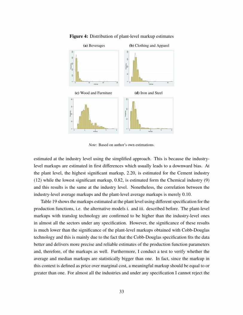
Figure 4: Distribution of plant-level markup estimates

(a) Beverages

010

020

030

040

050

0F

requ

ency

0 10 20 30markup

(b) Clothing and Apparel

050

100

150

200

Fre

quen

cy

0 5 10markup

(c) Wood and Furniture

020

4060

80F

requ

ency

0 1 2 3 4markup

(d) Iron and Steel

050

100

150

Fre

quen

cy

0 2 4 6 8markup

Note: Based on author’s own estimations.

estimated at the industry level using the simplified approach. This is because the industry-level markups are estimated in first differences which usually leads to a downward bias. Atthe plant level, the highest significant markup, 2.20, is estimated for the Cement industry(12) while the lowest significant markup, 0.82, is estimated form the Chemical industry (9)and this results is the same at the industry level. Nonetheless, the correlation between theindustry-level average markups and the plant-level average markups is merely 0.10.

Table 19 shows the markups estimated at the plant level using different specification for theproduction functions, i.e. the alternative models i. and iii. described before. The plant-levelmarkups with translog technology are confirmed to be higher than the industry-level onesin almost all the sectors under any specification. However, the significance of these resultsis much lower than the significance of the plant-level markups obtained with Cobb-Douglastechnology and this is mainly due to the fact that the Cobb-Douglas specification fits the databetter and delivers more precise and reliable estimates of the production function parametersand, therefore, of the markups as well. Furthermore, I conduct a test to verify whether theaverage and median markups are statistically bigger than one. In fact, since the markup inthis context is defined as price over marginal cost, a meaningful markup should be equal to orgreater than one. For almost all the industries and under any specification I cannot reject the

33

null hypothesis that the markups are statistically bigger than one at a 5 percent significancelevel. This result, though, needs to be considered cautiously because the confidence intervalsobtained by block-bootstrap used for inference are not very tight.

In conclusion, the striking differences between the industry-level and plant-level markupestimates, as summarized in table 18, highlight the following important point. Relaxing theconstant markup assumption across firms and allowing for time varying and heterogeneousproductivity shocks leads to more precise and substantially higher markups.

6.3 Markups, Trade Liberalization, and Export Status

In this section I study in detail the linkages between markups and trade. First, I rely on themodels described in section 3.2 to analyze the impact of trade liberalization on the price-costmargins at the industry and plant level. Then, I focus on characterizing the relation betweenmarkups and export status. Moreover, since the structural framework allows for estimatingboth markups and productivity at the plant level, I further explore the role of productivity inthe profitability of the Mexican manufacturing plants.

6.3.1 Industry-Level Analysis

To perform the industry-level analysis I use the results of the markups estimation presentedin section 6.1 obtained with the simple dual approach and the results obtained with thestructural approach estimating a Cobb-Douglas technology and using investment as a proxyfor productivity. In fact, only these two sets of results are directly comparable since one of therequirements to estimate (2.27) is for the production function to be linearly homogeneous andthe test on the returns to scale of the Cobb-Douglas production function in (2.11) confirmedthat there is statistically significant evidence of constant returns to scale in most of theindustries. Recall that the markups obtained with the simple dual approach are directlyestimated at the industry-level. On the other hand, the price-cost margins obtained with thestructural approach are estimated at the plant level, thus, in this part of the analysis, I collapsethese results to the annual average markup in each industry. The other explanatory variablesincluded in (3.1), i.e. Herfindahl index, capital-output ratio and measures of trade exposure,are constructed by aggregating and averaging across individual firms in each sector in eachyear. Models 1 and 2, which include industry-specific dummy variables, should explainthe temporal variation within each industry while models 3 and 4, with only year dummyvariables, are supposed to capture the variation between sectors. Note also that the measuresof trade exposure reflect the extent of trade liberalization, i.e. a decrease in the quota coverage

34

or in the tariff rate implies an increase in trade openness and foreign competition. Therefore,a positive coefficient associated with these trade indicators describes a negative effect of thetrade reforms on the markups and is expected in the presence of import discipline. Theregression results are reported separately for each type of trade liberalization instrument intables 20-23.

Tables 20 and 21 report the regression results obtained estimating (3.1) by OLS andusing the industry-level markups recovered with the simple dual approach as a dependentvariable. It is easy to see that, using either the quota coverage or the average tariff rateas trade indicators, very few coefficients in these regressions are significant and this resultis exacerbated in models 3 and 4 which include only year dummy variables. The lack ofsignificance is further confirmed by the adjusted R2 which is quite low, although all themodels are globally significant as verified by the F-statistic.

In both cases, with quota and tariff, one of the few significant coefficients is the oneassociated with the capital-output ratio in models 1 and 2. The sign of this coefficient isunexpectedly negative. However, since only the temporal variation is picked up in the modelwith industry dummy variables, this result may be reflecting underutilization of installedcapacity during the recession, which was prevalent for most of the sample period. As forthe measures of trade exposure, the coefficient associated with the tariff rate (table 21, model3) is positive and highly significant indicating that the markups tend to be lower the morethe openness to trade is. The coefficient on the interaction term between the trade indicatorand the capital-output ratio in model 2 is also consistently significant with both quota andtariff. Its positive sign is again evidence of trade discipline and suggests that industrieswith a higher capital-output ratio are more likely to experience a reduction in margins as aconsequence of trade liberalization. Nonetheless, because of the overall very low explanatorypower, the regression results reported in tables 20 and 21 cannot be viewed as strong evidenceof an impact of trade on the markups. In addition, these results confirm that the simple dualapproach used to obtain the markups at the industry level is inadequate since the markupestimates are imprecise, and in many cases insignificant, and this compromises any furtheranalysis conducted with those estimates.

I now turn to the regressions reported in tables 22 and 23 whose results are also obtainedestimating (3.1) by OLS with the annual average markup in each sector, recovered from thestructural plant-level estimation, as dependent variable. First, note that in these regressionsthe level of significance is substantially higher, especially when the industry dummy variablesare included (models 1 and 2). Thus, even if aggregated at the industry level, the markupscoming from the structural estimation appear to perform much better. However, a substantial

35

part of the explanatory power comes from industry effects as demonstrated by the R2 whichgreatly increases from models 3 and 4 to models 1 and 2. This outcome possibly reflectssector-specific industrial characteristics, policies, entry barriers or technological differencesthat are not captured by the other explanatory variables considered. The year effects arealways negative, with both quota and tariff, in model 1 and 2 and are also negative in models 3and 4 for the majority of the years considered. This result may capture the fact that during theperiod of analysis the Mexican economy faced difficult challenges that negatively impactedfirm profitability. The industry dummy variables, when included, are significant in manyindustries and their sign are consistent across all the specifications.

When quota is used as a trade indicator, the coefficient on the capital-output ratio has theexpected positive sign in everymodel and inmodel 3 and 4 it is also highly significant, implyingthat industries with a higher capital share of output have higher price-cost margins. On theother hand, when tariff is used as a measure of trade exposure, this coefficient is still positiveand significant when industry dummies are left out, but turns negative, although insignificant,when industry effects are controlled for. The coefficient associated with the Herfindahl index,when significant (model 3 with both quota and tariff) is positive confirming a higher rate ofprofitability in more concentrated industries. The coefficients on quota coverage and tariffrate are both positive and significant in model 3 indicating that price-cost margins decrease astrade protections are removed. In model 1, however, the same coefficients are not significant,suggesting that differences in the level of protection across sectors seem to be more relevantthan variation over time. Adding interaction terms reveals a more complex picture. The netimpact of quota coverage and tariff rate as well as their interaction with the Herfindahl indexand the capital-output ratio are not significant in explaining the temporal variation (model 2),but the interaction between quota and Herfindahl index (table 22, model 4) and the interactionbetween tariff and capital-output ratio (table 23, model 4) are significant. Specifically, theinteraction term for quota coverage and Herfindahl index is positive and significant implyingthat the profitability of the most concentrated industries is likely to decrease when trade isliberalized. Conversely, the interaction term for tariff rate and capital-output ratio in negativeand highly significant suggesting that the trade reforms have a negative impact on the marginsof the industry with the lowest capacity.

In summary, the industry-level analysis provides some evidence of import discipline,i.e. lower protection generated lower profitability in the Mexican manufacturing industries.This pattern is clearly established across sectors but not as clearly over time. Moreover, theimportance of using reliable estimates (in this case markups) to correctly evaluate economicpolicies is emphasized by the much better performance of the markups estimated within the

36

structural framework with respect to the ones estimated relying on the simpler dual approach.

6.3.2 Plant-Level Analysis

To examine the intra-sectoral variation in price-cost margins I estimate (3.2) by OLS usingthe plant-level markups as the dependent variable. Recall that these markups were recoveredfrom the structural estimation of my preferred specification, i.e. Cobb-Douglas technologywith investment as a proxy for productivity. The explanatory variables are also calculatedat the plant level with the exception of the trade indicators, quota coverage in model 1 andaverage tariff rate in model 2, which are only available at the industry level. The regressionresults are reported in table 24.

First note that the plant-level models are globally significant as indicated by the F-statistic,but explain only a small fraction of the plant-level variation in price-cost margins as confirmedby the relatively low value of the adjusted R2 (approximately 0.13). This is nonetheless acommon outcome of regressions performed on large micro-level dataset as the one used here.The year dummy variables are always negative but insignificant while the industry dummyvariables are significant in many cases with both positive and negative signs.

The coefficient associated with market share is positive and highly significant suggestingthat a rise in its market share increases the price-cost margin of a plant but at a decreasingrate, since the coefficient on the squared share is negative and significant, conversely. Thecoefficient on capital-output ratio is positive and highly significant in both models implyingthat, as expected, an increase in capacity has a positive effect on the profitability of a plant,however this effect becomes marginal when the capacity is large, as demonstrated by thevery small magnitude of the coefficient on the squared capital-output ratio. As for the tradeindicators, the coefficients on quota coverage and tariff rate are both insignificant, implyingthat there is no evidence that the trade reforms affected the price-cost margins of the Mexicanmanufacturing plants.19

I also estimate the same regressions with the plant-level markups obtained under differentspecifications, i.e. translog technology with both investment and intermediate inputs demandas proxies for productivity, as dependent variable. The results, not reported here, are in linewith those presented in table 24. However, the overall significance of the models is lower,presumably because, as already mentioned, the translog production function specificationdelivers imprecise and noisy markup estimates.

19A similar result is found in Grether (1996).

37

6.3.3 Markups for Exporters

To characterize the relation between markups and export status I first estimate (3.3) by OLSusing the logarithms of the plant-level markups estimated using my preferred specification,i.e. Cobb-Douglas technology with investment as a proxy for productivity, as the dependentvariable. The explanatory variables are capital and labor use, a full interaction of year andindustry dummy variables, and, of course, a dummy variable indicating export status. Afterobtaining an estimate for the coefficient associated with the exporter dummy ψ1, and theconstant term ψ0, I perform a test on the significance of the nonlinear combination of theparametersψ1+exp(ψ0)which captures the level markup difference for exporters. Finally, I re-estimate (3.3) adding the estimated productivity ω jt in order to directly control for differencesin productivity and verify whether there is still evidence of a markup premium for exporter.Specifically, the second regression is given by: ln(µ jt) = ψ0 + ψ1E jt + ψ2ω jt + z jtρ + ε jt .

In both cases, with and without the additional productivity control, I obtain that the thelevel markup difference µE = ψ1 + exp(ψ0) is positive, 0.019 not controlling for productivityand 0.016 controlling for productivity, respectively, but insignificant. However, since thenumber of exporting firms in the Mexican manufacturing industries is not very high in theyears considered and, most importantly, the extent of exporting is quite limited for the majorityof the exporters, I try to verify whether the markup premium exists for intensive exporters, i.e.firms that export a high percentage of the value of their output. To do so I calculate for eachexporter the ratio of exports value over output value and substitute the export dummy in (3.3)with another dummy, EHjt , that indicates export intensity. Specifically, EHjt is equal to one iffirm j is in the 75th or above percentile of the export-output ratio distribution, i.e. if firm j isan intensive exporter. Table 25 shows the results obtained estimating the modified version of(3.3) by OLS with the export intensity dummy, not controlling (model 1) and controlling forproductivity (model 2).

First, the coefficient associated with the export intensity dummy variable is always positiveand significant, with and without including productivity in the regression, suggesting thatexporting has a positive impact on price-cost margins. Also, the coefficient associatedwith productivity in model 2 is positive and highly significant, meaning that productivitycontributes to firms’ profitability. In addition, the level markup difference for intensiveexporters µEH is positive and significant in bothmodels. More precisely, I obtain a significantlyestimated µEH of 0.0588 inmodel 1 which implies that intensive exporters have a level markuppremium of approximately 6 percent. In model 2 the estimated µEH is significant and equalto 0.0539, meaning that, even controlling for productivity, the intensive exporter have a

38

level markup premium of approximately 5.4 percent. Note that controlling for productivityin this context means to control for differences in marginal costs, if ψ2 (the coefficient onproductivity) picks up cost heterogeneity fully, so that the coefficient on the intensive exporterdummy picks up the variation in average prices between intensive exporter and the other firms(low exporters and non exporters). However, because the productivity used in this regressionwas estimated as the residual of a value added production function, it may not contain onlydifferences in costs but also unobserved quality differences in both inputs and output, as wellas others market power effects. Nonetheless, it is important to emphasize that an intensiveexporter effect is still present, even once differences in productivity are accounted for. Thisresult is therefore consistent with the recent international trade literature predicting a positiverelation between markups and exports status, especially in the case of intensive exporters.

6.3.4 Reconciling Industry- and Plant-level Evidence

As already mentioned, the exercise performed in this paper demonstrates the importanceof relying on accurate and precise estimates when evaluating the effects of a policy. Forthis reason, the results reported in tables 20 and 21 are not to be trusted because they arebased on implausible and insignificant markup estimates. However, even considering onlyfirm-specific markups, the analysis conducted at the plant level delivers different resultsthan the analysis at the industry level. How can this evidence be reconciled to understandand assess the effectiveness of trade liberalization in reducing market power in the Mexicanmanufacturing industries? Specifically, what can rationalize the fact that trade liberalizationdid not significantly reduce price-cost margins at the plant level but seems to have affectedthem at the industry level? Moreover, why are intensive exporters different?

Possible answers to these questions lie in the selection mechanism characterized in recenttrade models.20 The key insight of these models is that, if trade exposure does not change thebehavior of the single firm, but simply the selection of the firms that are able to stay in themarket, a direct effect of trade liberalization at the firm level would not be observed, but itcould be observed at the industry level because of changes in the intra-industry composition.In this case, the lack of trade discipline evidence at the plant level is consistent with theidea that Mexican firms were not prompted to charge lower markups as a consequenceof trade liberalization. Nonetheless, if the substantial decrease in protection from foreigncompetition generated intra-industry selection among firms forcing those that were charginghigher markups to exit, and possibly be substituted by lower-profitability firms, the effect of

20See Melitz (2003).

39

trade liberalization would manifest in lower industry-level markups. In addition, the selectionprocess works through the productivity channel inducing the most productive firms to becomeexporters, which, as discussed before, are able to enjoy a markup premium. Since exporters,and especially intensive exporters, represent a very small fraction of the total firms consideredin the analysis, it is reasonable to observe that their higher-profitability status is relevantand significant, yet not enough to offset the overall effect determined by the intra-industryselection of low-profitability firms.

7 Conclusions

In this contribution I focus on the importance of correctly estimating production functionparameters and price-cost margins in order to assess differences in technology, productivity,and market power among eighteen Mexican manufacturing firms and evaluate the impact oftrade liberalizing policies on their profitability.

I estimate production function parameters relying on a structural framework that correctsfor the simultaneity bias using investment or intermediate inputs as a proxy for unobservedproductivity. My results confirm thewell establish empirical evidence that production functioncoefficients obtained with OLS are biased and support the argument that controlling for firm-specific productivity shocks corrects this bias. In fact, compared to OLS, the structuralestimation delivers a much lower labor parameter and a higher capital parameter. I also findevidence of constant returns to scale in the majority of the industries analyzed.

The second step in my empirical investigation consists of using the production functionestimates to recover firm-level markups adopting a structural approach in which markups arederived from cost minimization first order conditions and can be interpreted as the wedgebetween the cost share of production factors and their revenue share. I test the validity of thisapproach by comparing the firm-level markup estimates with industry-level markups obtainedthrough a less sophisticated dual estimation approach. The price cost-margins estimated atthe plant level are more reasonable in terms of magnitude and significantly higher thantheir industry-level counterparts. This result demonstrates that explicitly taking into accountdifferences in productivity is crucial in assessing the extent of market power.

Finally, I exploit the fact that the sample spans over a period of dramatic reforms in theMexican economy to quantify the impact of trade exposure on the markups. I conduct anindustry-level as well as a plant-level analysis relating price-cost margins and measures ofimport liberalization. The industry-level evidence seems to support the hypothesis of import

40

discipline, i.e. the removal of trade protections negatively affected the profitability of domesticfirms, but this evidence is not confirmed in the plant-level analysis. In addition, I test theprediction that larger firms are likely to be more productive, thus can charge higher markupsand afford to pay a sunk cost to become exporters. In the case of Mexican exporters I find astatistically significant markup premium only for intensive exporters, i.e. firms that export ahigh percentage of their output, and for these firms the premium persists even after netting outthe effect of productivity. This evidence is consistent with recent international trade modelspredicting that trade exposure does not necessarily change the behavior of the single firmbut induces a selection of firms modifying the intra-industry composition. Productivity iscertainly an important channel through which the selection mechanism works allowing themost productive firms to become exporters and to be, on average, more profitable.

Since the trade liberalization of the late 1980s analyzed in this paper, Mexico has becomeeven more open and integrated in production value chains by joining the North AmericanFree Trade Agreement (NAFTA) in 1994. NAFTA created one of the world’s largest freetrade zones and was supposed to lay the foundations for strong economic growth and risingprosperity for its members. While the period after the enactment of NAFTA, and beforeChina’s admission to the World Trade Organization, was associated with an above-averageGDP growth in Mexico, it is difficult to determine the extent to which this was the result offirms becoming more productive. The exposure to trade should have boosted competitionand created greater incentives for innovation and productivity improvements, yet the evidenceof such improvements is limited. In addition, in more recent years, Mexico’s exportingperformance has been impressively strong, especially to the United States, but the overalleconomy has experienced a rather sluggish GDP growth. All these considerations suggestthat the effectiveness of trade policies crucially depends on the ability of implementingcomplementary reforms aimed at the internal market that promote competition, eliminatedistortions in the allocation of resources, and stimulate investments in innovation and growth.Especially in times of great uncertainty, such as the current ones regarding the future ofNAFTA, focusing on building a solid, competitive, and productive domestic economy is ofparamount importance for Mexico’s prosperity.

41

References

Ackerberg, D., Benkard, C. L., Berry, S., & Pakes, A. (2007). Econometric tools for analyzingmarket outcomes. In Handbook of econometrics (Vol. 6, pp. 4171–4276). Elsevier.

Ackerberg, D., Cavez, K., & Frazer, G. (2015). Identification properties of recent productionfunction estimators. Econometrica, 83(6), 2411–2451.

Bernard, A. B., Eaton, J., Jensen, J. B., & Kortum, S. (2003). Plants and productivity ininternational trade. The American Economic Review, 93(4), 1268–1290.

Bloom, N., & Van Reenen, J. (2007). Measuring and explaining management practices acrossfirms and countries. The Quarterly Journal of Economics, 122(4), 1351–1408.

Bloom, N., & Van Reenen, J. (2010). Why do management practices differ across firms andcountries? Journal of Economic Perspectives, 24(1), 203–24.

Blundell, R., & Bond, S. (2000). Gmm estimation with persistent panel data: an applicationto production functions. Econometric Reviews, 19(3), 321–340.

Chamberlain, G. (1982). Multivariate regression models for panel data. Journal of Econo-metrics, 18(1), 5–46.

Cobb, C. W., & Douglas, P. H. (1928). A theory of production. The American EconomicReview, 18(1), 139–165.

De Loecker, J., & Eeckhout, J. (2017). The rise of market power and the macroeconomicimplications. National Bureau of Economic Research Working Paper No. 23687.

De Loecker, J., & Eeckhout, J. (2018). Some thoughts on the debate about (aggregate) markupmeasurement. UPF-GSE Barcelona, mimeo.

De Loecker, J., & Warzynski, F. (2012). Markups and firm-level export status. The AmericanEconomic Review, 102(6), 2437–2471.

Demsetz, H. (1973). Industry structure, market rivalry, and public policy. The Journal ofLaw and Economics, 16(1), 1–9.

Domowitz, I., Hubbard, R. G., & Petersen, B. C. (1986). Business cycles and the relationshipbetween concentration and price-cost margins. The RAND Journal of Economics, 1–17.

Doraszelski, U., & Jaumandreu, J. (2013). R&d and productivity: Estimating endogenousproductivity. Review of Economic Studies, 80(4), 1338–1383.

Grether, J.-M. (1996). Mexico, 1985-90: Trade liberalization, market structure, and man-ufacturing performance. In M. Roberts & J. Tybout (Eds.), Industrial evolution indeveloping countries (pp. 260–283). Oxford University Press.

Griliches, Z., & Mairesse, J. (1995). Production functions: the search for identification.National Bureau of Economic Research Working Paper No. 5067.

42

Hall, R. (2018). Using empirical marginal cost to measure market power in the US economy.National Bureau of Economic Research Working Paper No. 25251.

Hall, R., Blanchard, O., & Hubbard, G. (1986). Market structure and macroeconomicfluctuations. Brookings Papers on Economic Activity, 1986(2), 285–338.

Hall, R. E. (1988). The relation between price and marginal cost in US industry. Journal ofPolitical Economy, 96(5), 921–947.

Hallak, J. C., & Sivadasan, J. (2013). Product and process productivity: Implications forquality choice and conditional exporter premia. Journal of International Economics,91(1), 53–67.

Hoch, I. (1955). Estimation of production function parameters and testing for efficiency.Econometrica, 23(3), 325–26.

Hoch, I. (1962). Estimation of production function parameters combining time-series andcross-section data. Econometrica: Journal of the Econometric Society, 34–53.

Horowitz, J. L. (2001). The bootstrap. InHandbook of econometrics (Vol. 5, pp. 3159–3228).Elsevier.

Hsieh, C.-T., & Klenow, P. J. (2009). Misallocation and manufacturing TFP in China andIndia. The Quarterly Journal of Economics, 124(4), 1403–1448.

Kehoe, T. J. (1995). A review of Mexico’s trade policy from 1982 to 1994. World Economy,18, 135–135.

Klette, T. J., & Griliches, Z. (1996). The inconsistency of common scale estimators whenoutput prices are unobserved and endogenous. Journal of Applied Econometrics, 343–361.

Krishna, P., & Mitra, D. (1998). Trade liberalization, market discipline and productivitygrowth: new evidence from India. Journal of Development Economics, 56(2), 447–462.

Kugler, M., & Verhoogen, E. (2011). Prices, plant size, and product quality. The Review ofEconomic Studies, 79(1), 307–339.

Levinsohn, J., & Petrin, A. (2003). Estimating production functions using inputs to controlfor unobservables. The Review of Economic Studies, 70(2), 317–341.

Marschak, J., & Andrews, W. H. (1944). Random simultaneous equations and the theory ofproduction. Econometrica, 12(3/4), 143–205.

Melitz, M. J. (2003). The impact of trade on intra-industry reallocations and aggregateindustry productivity. Econometrica, 71(6), 1695–1725.

Melitz, M. J., & Ottaviano, G. I. (2008). Market size, trade, and productivity. The Review ofEconomic Studies, 75(1), 295–316.

43

Mundlak, Y. (1961). Empirical production function free of management bias. Journal ofFarm Economics, 43(1), 44–56.

Nerlove,M. (1963). Returns to scale in electricity supply. In C. F. Christ (Ed.),Measurement ineconomics. Studies in mathematical economics and econometrics in memory of YehudaGrunfeld (Vol. 197). Stanford University Press.

Olley, G. S., & Pakes, A. (1996). The dynamics of productivity in the telecommunicationsequipment. Econometrica, 64(6), 1263–1297.

Pavcnik, N. (2002). Trade liberalization, exit, and productivity improvements: Evidence fromChilean plants. The Review of Economic Studies, 69(1), 245–276.

Roeger, W. (1995). Can imperfect competition explain the difference between primal and dualproductivity measures? estimates for US manufacturing. Journal of Political Economy,103(2), 316–330.

Schmalensee, R. (1985). Do markets differ much? The American Economic Review, 75(3),341–351.

Tybout, J. R.,&Westbrook,M.D. (1995). Trade liberalization and the dimensions of efficiencychange inMexicanmanufacturing industries. Journal of International Economics, 39(1-2), 53–78.

44

Table 1: Variables from the original dataset used in the analysis

Variable DescriptionLabor forceTOTREMUN1 total labor remunerationsTOHHOM1 total hours workedTOPEOC total employment

Inputs costsTOTMASUM5 total material costGTRENALQ1 rent and leasing costsVAENELCN6 value of electricity consumedGASTMAQU1 cost of subcontractors

Value of outputVALPROEL2 value of output

RevenueINSERMAQ1 income from subcontracting

Fixed capitalV684 machinery and equipment valued at replacement costV924 machinery and equipment produced for own useV693 construction and installation valued at replacement costV933 construction and install assets produced for own useV701 land valued at replacement costV717 transportation equipment valued at replacement costV947 transportation equipment assets produced for own useV721 other assets valued at replacement costV954 other asset produced for own use

Trade indicatorsTAI630 average tariff on input (June 30)TAI1230 average tariff on input (Dec. 30)TAQ630 average tariff on output (June 30)TAQ1230 average tariff on output (Dec. 30)LCI630 license coverage on input (June 30)LCI1230 license coverage on input (Dec. 30)LCQ630 license coverage on output (June 30)LCQ1230 license coverage on output (Dec. 30)

Price indices1PM wholesale price index2PPP producer price index3PKE construction price index4PK machinery price index5PMP1 raw materials price index6PEMP electricity price index7PKT transportation price index

Note: Based on variable codes from INEGI’s Annual Industrial Survey provided by the former Mex-ican Secretariat of Commerce and Industrial Development.

45

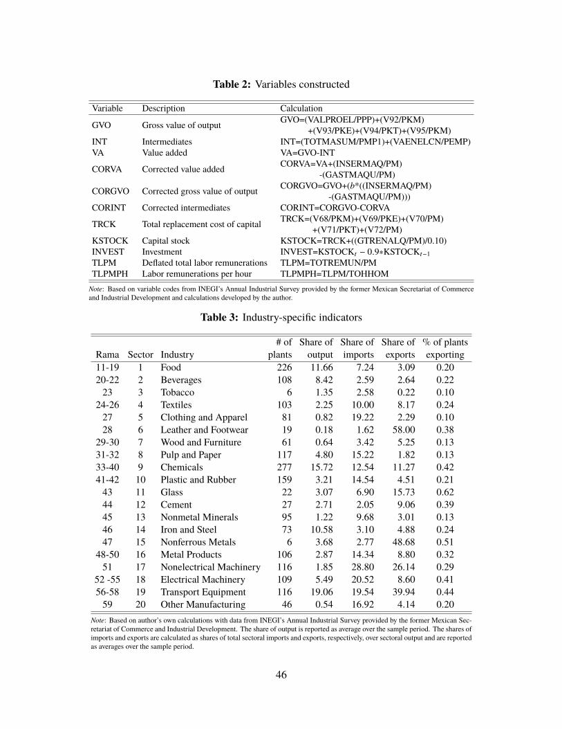
Table 2: Variables constructed

Variable Description Calculation

GVO Gross value of output GVO=(VALPROEL/PPP)+(V92/PKM)+(V93/PKE)+(V94/PKT)+(V95/PKM)

INT Intermediates INT=(TOTMASUM/PMP1)+(VAENELCN/PEMP)VA Value added VA=GVO-INT

CORVA Corrected value added CORVA=VA+(INSERMAQ/PM)-(GASTMAQU/PM)

CORGVO Corrected gross value of output CORGVO=GVO+(b*((INSERMAQ/PM)-(GASTMAQU/PM)))

CORINT Corrected intermediates CORINT=CORGVO-CORVA

TRCK Total replacement cost of capital TRCK=(V68/PKM)+(V69/PKE)+(V70/PM)+(V71/PKT)+(V72/PM)

KSTOCK Capital stock KSTOCK=TRCK+((GTRENALQ/PM)/0.10)INVEST Investment INVEST=KSTOCKt − 0.9∗KSTOCKt−1TLPM Deflated total labor remunerations TLPM=TOTREMUN/PMTLPMPH Labor remunerations per hour TLPMPH=TLPM/TOHHOMNote: Based on variable codes from INEGI’s Annual Industrial Survey provided by the former Mexican Secretariat of Commerceand Industrial Development and calculations developed by the author.

Table 3: Industry-specific indicators

# of Share of Share of Share of % of plantsRama Sector Industry plants output imports exports exporting11-19 1 Food 226 11.66 7.24 3.09 0.2020-22 2 Beverages 108 8.42 2.59 2.64 0.2223 3 Tobacco 6 1.35 2.58 0.22 0.10

24-26 4 Textiles 103 2.25 10.00 8.17 0.2427 5 Clothing and Apparel 81 0.82 19.22 2.29 0.1028 6 Leather and Footwear 19 0.18 1.62 58.00 0.38

29-30 7 Wood and Furniture 61 0.64 3.42 5.25 0.1331-32 8 Pulp and Paper 117 4.80 15.22 1.82 0.1333-40 9 Chemicals 277 15.72 12.54 11.27 0.4241-42 10 Plastic and Rubber 159 3.21 14.54 4.51 0.2143 11 Glass 22 3.07 6.90 15.73 0.6244 12 Cement 27 2.71 2.05 9.06 0.3945 13 Nonmetal Minerals 95 1.22 9.68 3.01 0.1346 14 Iron and Steel 73 10.58 3.10 4.88 0.2447 15 Nonferrous Metals 6 3.68 2.77 48.68 0.51

48-50 16 Metal Products 106 2.87 14.34 8.80 0.3251 17 Nonelectrical Machinery 116 1.85 28.80 26.14 0.29

52 -55 18 Electrical Machinery 109 5.49 20.52 8.60 0.4156-58 19 Transport Equipment 116 19.06 19.54 39.94 0.4459 20 Other Manufacturing 46 0.54 16.92 4.14 0.20

Note: Based on author’s own calculations with data from INEGI’s Annual Industrial Survey provided by the former Mexican Sec-retariat of Commerce and Industrial Development. The share of output is reported as average over the sample period. The shares ofimports and exports are calculated as shares of total sectoral imports and exports, respectively, over sectoral output and are reportedas averages over the sample period.

46

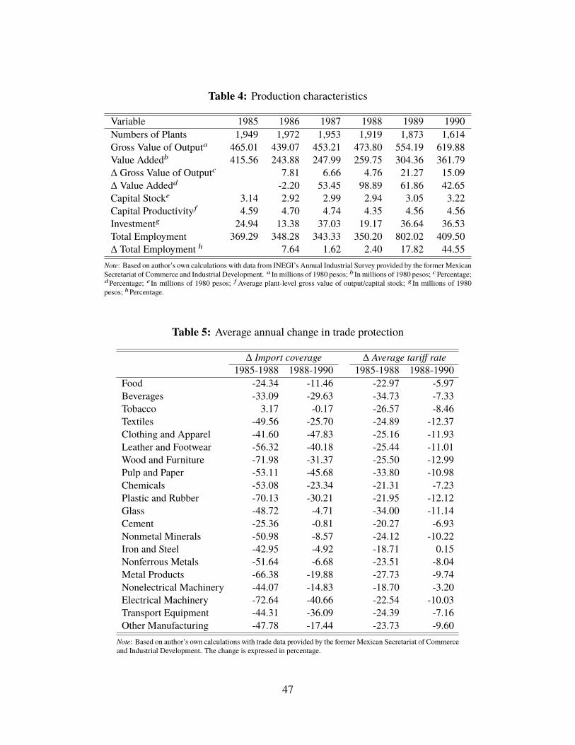
Table 4: Production characteristics

Variable 1985 1986 1987 1988 1989 1990Numbers of Plants 1,949 1,972 1,953 1,919 1,873 1,614Gross Value of Outputa 465.01 439.07 453.21 473.80 554.19 619.88Value Addedb 415.56 243.88 247.99 259.75 304.36 361.79∆ Gross Value of Outputc 7.81 6.66 4.76 21.27 15.09∆ Value Addedd -2.20 53.45 98.89 61.86 42.65Capital Stocke 3.14 2.92 2.99 2.94 3.05 3.22Capital Productivity f 4.59 4.70 4.74 4.35 4.56 4.56Investmentg 24.94 13.38 37.03 19.17 36.64 36.53Total Employment 369.29 348.28 343.33 350.20 802.02 409.50∆ Total Employment h 7.64 1.62 2.40 17.82 44.55

Note: Based on author’s own calculations with data from INEGI’s Annual Industrial Survey provided by the former MexicanSecretariat of Commerce and Industrial Development. a In millions of 1980 pesos; b In millions of 1980 pesos; cPercentage;dPercentage; e In millions of 1980 pesos; f Average plant-level gross value of output/capital stock; g In millions of 1980pesos; hPercentage.

Table 5: Average annual change in trade protection

∆ Import coverage ∆ Average tariff rate1985-1988 1988-1990 1985-1988 1988-1990

Food -24.34 -11.46 -22.97 -5.97Beverages -33.09 -29.63 -34.73 -7.33Tobacco 3.17 -0.17 -26.57 -8.46Textiles -49.56 -25.70 -24.89 -12.37Clothing and Apparel -41.60 -47.83 -25.16 -11.93Leather and Footwear -56.32 -40.18 -25.44 -11.01Wood and Furniture -71.98 -31.37 -25.50 -12.99Pulp and Paper -53.11 -45.68 -33.80 -10.98Chemicals -53.08 -23.34 -21.31 -7.23Plastic and Rubber -70.13 -30.21 -21.95 -12.12Glass -48.72 -4.71 -34.00 -11.14Cement -25.36 -0.81 -20.27 -6.93Nonmetal Minerals -50.98 -8.57 -24.12 -10.22Iron and Steel -42.95 -4.92 -18.71 0.15Nonferrous Metals -51.64 -6.68 -23.51 -8.04Metal Products -66.38 -19.88 -27.73 -9.74Nonelectrical Machinery -44.07 -14.83 -18.70 -3.20Electrical Machinery -72.64 -40.66 -22.54 -10.03Transport Equipment -44.31 -36.09 -24.39 -7.16Other Manufacturing -47.78 -17.44 -23.73 -9.60

Note: Based on author’s own calculations with trade data provided by the former Mexican Secretariat of Commerceand Industrial Development. The change is expressed in percentage.

47

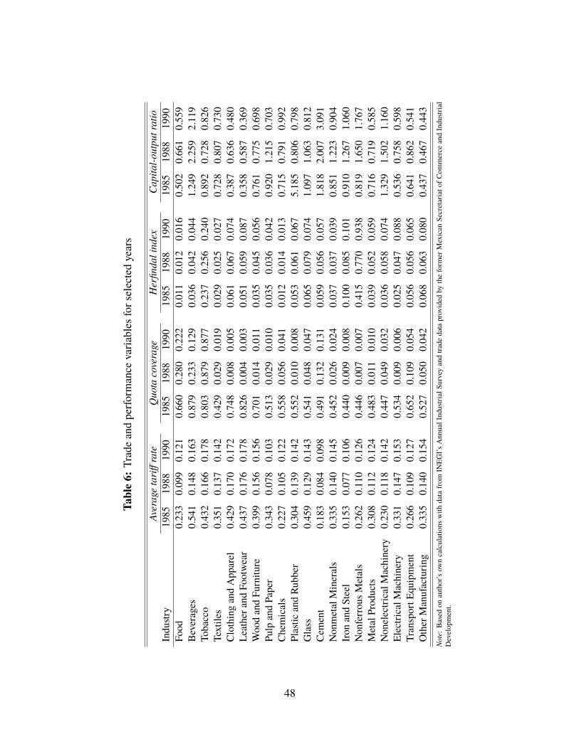
Table6:

Tradeandperfo

rmance

varia

bles

forselectedyears

Averagetariffrate

Quota

coverage

Herfin

dalind

exCap

ital-o

utpu

tratio

Indu

stry

1985

1988

1990

1985

1988

1990

1985

1988

1990

1985

1988

1990

Food

0.23

30.09

90.12

10.66

00.28

00.22

20.01

10.01

20.01

60.50

20.66

10.55

9Beverages

0.54

10.14

80.16

30.87

90.23

30.12

90.03

60.04

20.04

41.24

92.25

92.11

9To

bacco

0.43

20.16

60.17

80.80

30.87

90.87

70.23

70.25

60.24

00.89

20.72

80.82

6Textile

s0.35

10.13

70.14

20.42

90.02

90.01

90.02

90.02

50.02

70.72

80.80

70.73

0ClothingandApp

arel

0.42

90.17

00.17

20.74

80.00

80.00

50.06

10.06

70.07

40.38

70.63

60.48

0Le

athera

ndFo

otwear

0.43

70.17

60.17

80.82

60.00

40.00

30.05

10.05

90.08

70.35

80.58

70.36

9Woo

dandFu

rnitu

re0.39

90.15

60.15

60.70

10.01

40.01

10.03

50.04

50.05

60.76

10.77

50.69

8Pu

lpandPaper

0.34

30.07

80.10

30.51

30.02

90.01

00.03

50.03

60.04

20.92

01.21

50.70

3Chemicals

0.22

70.10

50.12

20.55

80.05

60.04

10.01

20.01

40.01

30.71

50.79

10.99

2Plastic

andRu

bber

0.30

40.13

90.14

20.55

20.01

00.00

80.05

30.06

10.06

75.18

50.80

60.79

8Glass

0.45

90.12

90.14

30.54

10.04

80.04

70.06

50.07

90.07

41.09

71.06

30.81

2Cem

ent

0.18

30.08

40.09

80.49

10.13

20.13

10.05

90.05

60.05

71.81

82.00

73.09

1Non

metalMinerals

0.33

50.14

00.14

50.45

20.02

60.02

40.03

70.03

70.03

90.85

11.22

30.90

4Iron

andSteel

0.15

30.07

70.10

60.44

00.00

90.00

80.10

00.08

50.10

10.91

01.26

71.06

0Non

ferrou

sMetals

0.26

20.11

00.12

60.44

60.00

70.00

70.41

50.77

00.93

80.81

91.65

01.76

7MetalProd

ucts

0.30

80.11

20.12

40.48

30.01

10.01

00.03

90.05

20.05

90.71

60.71

90.58

5Non

electricalM

achinery

0.23

00.11

80.14

20.44

70.04

90.03

20.03

60.05

80.07

41.32

91.50

21.16

0ElectricalM

achinery

0.33

10.14

70.15

30.53

40.00

90.00

60.02

50.04

70.08

80.53

60.75

80.59

8TransportE

quipment

0.26

60.10

90.12

70.65

20.10

90.05

40.05

60.05

60.06

50.64

10.86

20.54

1Other

Manufacturin

g0.33

50.14

00.15

40.52

70.05

00.04

20.06

80.06

30.08

00.43

70.46

70.44

3No

te:Based

onauthor’sow

ncalculations

with

datafrom

INEG

I’sAnn

ualInd

ustrialSu

rvey

andtra

dedataprovided

bytheform

erMexican

Secretariato

fCom

merce

andIndu

strial

Develop

ment.

48

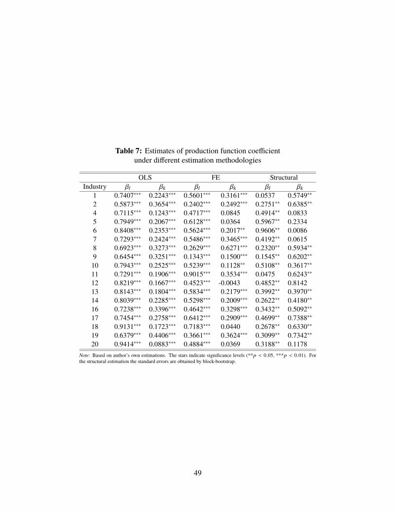
Table 7: Estimates of production function coefficientunder different estimation methodologies

OLS FE StructuralIndustry βl βk βl βk βl βk

1 0.7407∗∗∗ 0.2243∗∗∗ 0.5601∗∗∗ 0.3161∗∗∗ 0.0537 0.5749∗∗2 0.5873∗∗∗ 0.3654∗∗∗ 0.2402∗∗∗ 0.2492∗∗∗ 0.2751∗∗ 0.6385∗∗4 0.7115∗∗∗ 0.1243∗∗∗ 0.4717∗∗∗ 0.0845 0.4914∗∗ 0.08335 0.7949∗∗∗ 0.2067∗∗∗ 0.6128∗∗∗ 0.0364 0.5967∗∗ 0.23346 0.8408∗∗∗ 0.2353∗∗∗ 0.5624∗∗∗ 0.2017∗∗ 0.9606∗∗ 0.00867 0.7293∗∗∗ 0.2424∗∗∗ 0.5486∗∗∗ 0.3465∗∗∗ 0.4192∗∗ 0.06158 0.6923∗∗∗ 0.3273∗∗∗ 0.2629∗∗∗ 0.6271∗∗∗ 0.2320∗∗ 0.5934∗∗9 0.6454∗∗∗ 0.3251∗∗∗ 0.1343∗∗∗ 0.1500∗∗∗ 0.1545∗∗ 0.6202∗∗10 0.7943∗∗∗ 0.2525∗∗∗ 0.5239∗∗∗ 0.1128∗∗ 0.5108∗∗ 0.3617∗∗11 0.7291∗∗∗ 0.1906∗∗∗ 0.9015∗∗∗ 0.3534∗∗∗ 0.0475 0.6243∗∗12 0.8219∗∗∗ 0.1667∗∗∗ 0.4523∗∗∗ -0.0043 0.4852∗∗ 0.814213 0.8143∗∗∗ 0.1804∗∗∗ 0.5834∗∗∗ 0.2179∗∗∗ 0.3992∗∗ 0.3970∗∗14 0.8039∗∗∗ 0.2285∗∗∗ 0.5298∗∗∗ 0.2009∗∗∗ 0.2622∗∗ 0.4180∗∗16 0.7238∗∗∗ 0.3396∗∗∗ 0.4642∗∗∗ 0.3298∗∗∗ 0.3432∗∗ 0.5092∗∗17 0.7454∗∗∗ 0.2758∗∗∗ 0.6412∗∗∗ 0.2909∗∗∗ 0.4699∗∗ 0.7388∗∗18 0.9131∗∗∗ 0.1723∗∗∗ 0.7183∗∗∗ 0.0440 0.2678∗∗ 0.6330∗∗19 0.6379∗∗∗ 0.4406∗∗∗ 0.3661∗∗∗ 0.3624∗∗∗ 0.3099∗∗ 0.7342∗∗20 0.9414∗∗∗ 0.0883∗∗∗ 0.4884∗∗∗ 0.0369 0.3188∗∗ 0.1178

Note: Based on author’s own estimations. The stars indicate significance levels (**p < 0.05, ***p < 0.01). Forthe structural estimation the standard errors are obtained by block-bootstrap.

49

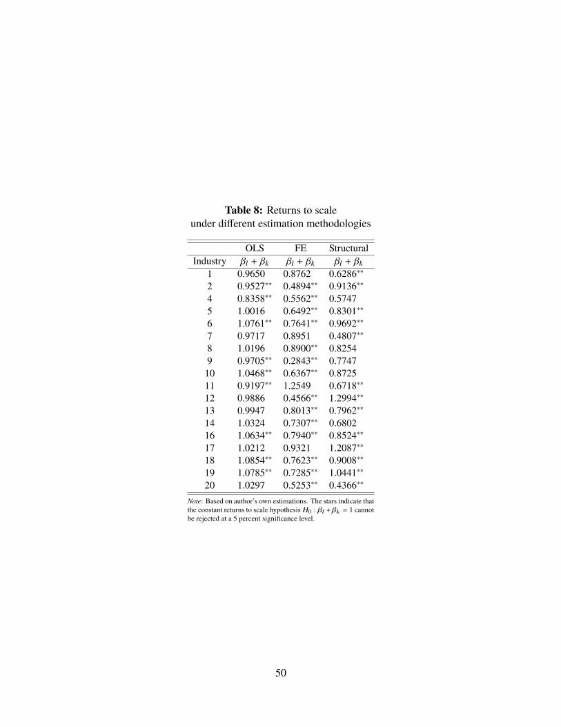
Table 8: Returns to scaleunder different estimation methodologies

OLS FE StructuralIndustry βl + βk βl + βk βl + βk

1 0.9650 0.8762 0.6286∗∗2 0.9527∗∗ 0.4894∗∗ 0.9136∗∗4 0.8358∗∗ 0.5562∗∗ 0.57475 1.0016 0.6492∗∗ 0.8301∗∗6 1.0761∗∗ 0.7641∗∗ 0.9692∗∗7 0.9717 0.8951 0.4807∗∗8 1.0196 0.8900∗∗ 0.82549 0.9705∗∗ 0.2843∗∗ 0.774710 1.0468∗∗ 0.6367∗∗ 0.872511 0.9197∗∗ 1.2549 0.6718∗∗12 0.9886 0.4566∗∗ 1.2994∗∗13 0.9947 0.8013∗∗ 0.7962∗∗14 1.0324 0.7307∗∗ 0.680216 1.0634∗∗ 0.7940∗∗ 0.8524∗∗17 1.0212 0.9321 1.2087∗∗18 1.0854∗∗ 0.7623∗∗ 0.9008∗∗19 1.0785∗∗ 0.7285∗∗ 1.0441∗∗20 1.0297 0.5253∗∗ 0.4366∗∗

Note: Based on author’s own estimations. The stars indicate thatthe constant returns to scale hypothesis H0 : βl +βk = 1 cannotbe rejected at a 5 percent significance level.

50

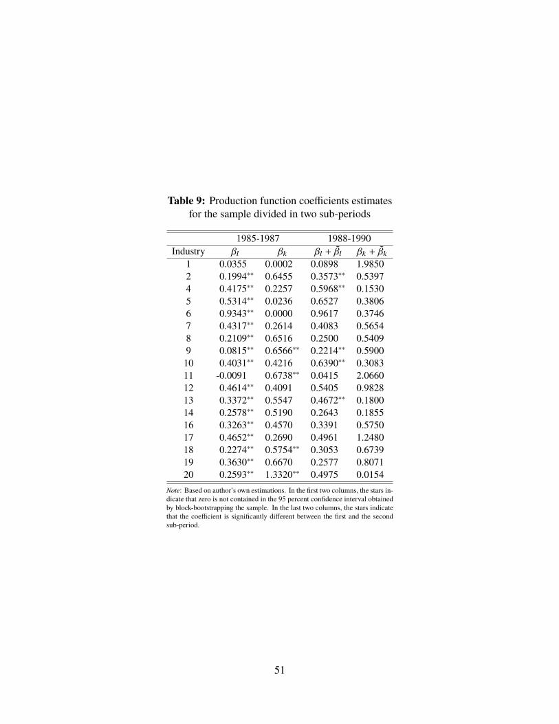
Table 9: Production function coefficients estimatesfor the sample divided in two sub-periods

1985-1987 1988-1990Industry βl βk βl + βl βk + βk

1 0.0355 0.0002 0.0898 1.98502 0.1994∗∗ 0.6455 0.3573∗∗ 0.53974 0.4175∗∗ 0.2257 0.5968∗∗ 0.15305 0.5314∗∗ 0.0236 0.6527 0.38066 0.9343∗∗ 0.0000 0.9617 0.37467 0.4317∗∗ 0.2614 0.4083 0.56548 0.2109∗∗ 0.6516 0.2500 0.54099 0.0815∗∗ 0.6566∗∗ 0.2214∗∗ 0.590010 0.4031∗∗ 0.4216 0.6390∗∗ 0.308311 -0.0091 0.6738∗∗ 0.0415 2.066012 0.4614∗∗ 0.4091 0.5405 0.982813 0.3372∗∗ 0.5547 0.4672∗∗ 0.180014 0.2578∗∗ 0.5190 0.2643 0.185516 0.3263∗∗ 0.4570 0.3391 0.575017 0.4652∗∗ 0.2690 0.4961 1.248018 0.2274∗∗ 0.5754∗∗ 0.3053 0.673919 0.3630∗∗ 0.6670 0.2577 0.807120 0.2593∗∗ 1.3320∗∗ 0.4975 0.0154

Note: Based on author’s own estimations. In the first two columns, the stars in-dicate that zero is not contained in the 95 percent confidence interval obtainedby block-bootstrapping the sample. In the last two columns, the stars indicatethat the coefficient is significantly different between the first and the secondsub-period.

51

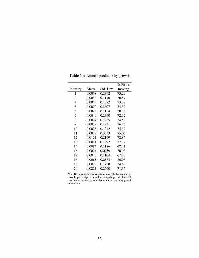
Table 10: Annual productivity growth

% FirmsIndustry Mean Std. Dev. moving

1 0.0078 0.2392 73.292 0.0048 0.1110 78.574 0.0005 0.1082 73.785 0.0022 0.2607 74.506 0.0042 0.1154 70.757 -0.0049 0.2390 72.128 -0.0027 0.1285 74.569 -0.0039 0.1231 76.4610 0.0006 0.1212 75.4911 0.0079 0.3033 85.0612 -0.0121 0.2199 78.8513 -0.0001 0.1292 77.1714 -0.0084 0.1186 67.4116 0.0004 0.0959 70.9317 0.0045 0.1164 67.2018 0.0065 0.2574 80.9819 0.0002 0.1728 74.8920 0.0221 0.2660 71.35

Note: Based on author’s own estimations. The last column re-ports the percentage of firms that during the period 1986-1990have moved across the quartiles of the productivity growthdistribution.

52

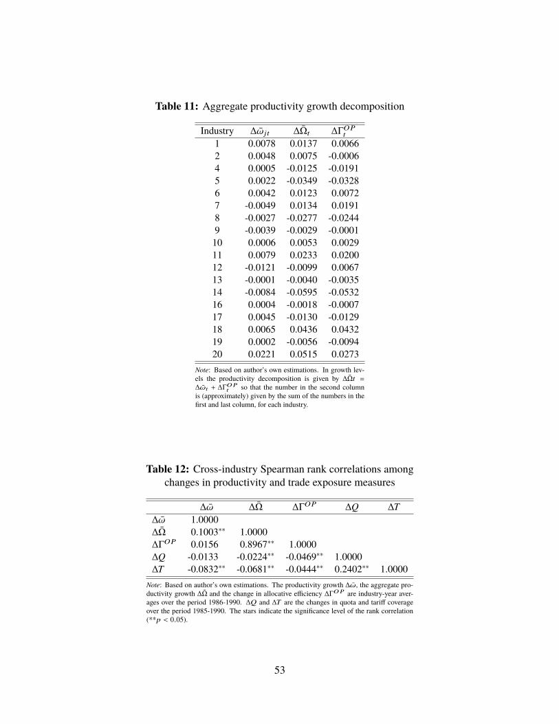
Table 11: Aggregate productivity growth decomposition

Industry ∆ωjt ∆Ωt ∆ΓOPt

1 0.0078 0.0137 0.00662 0.0048 0.0075 -0.00064 0.0005 -0.0125 -0.01915 0.0022 -0.0349 -0.03286 0.0042 0.0123 0.00727 -0.0049 0.0134 0.01918 -0.0027 -0.0277 -0.02449 -0.0039 -0.0029 -0.000110 0.0006 0.0053 0.002911 0.0079 0.0233 0.020012 -0.0121 -0.0099 0.006713 -0.0001 -0.0040 -0.003514 -0.0084 -0.0595 -0.053216 0.0004 -0.0018 -0.000717 0.0045 -0.0130 -0.012918 0.0065 0.0436 0.043219 0.0002 -0.0056 -0.009420 0.0221 0.0515 0.0273

Note: Based on author’s own estimations. In growth lev-els the productivity decomposition is given by ∆Ωt =∆ωt + ∆Γ

OPt so that the number in the second column

is (approximately) given by the sum of the numbers in thefirst and last column, for each industry.

Table 12: Cross-industry Spearman rank correlations amongchanges in productivity and trade exposure measures

∆ω ∆Ω ∆ΓOP ∆Q ∆T∆ω 1.0000∆Ω 0.1003∗∗ 1.0000∆ΓOP 0.0156 0.8967∗∗ 1.0000∆Q -0.0133 -0.0224∗∗ -0.0469∗∗ 1.0000∆T -0.0832∗∗ -0.0681∗∗ -0.0444∗∗ 0.2402∗∗ 1.0000

Note: Based on author’s own estimations. The productivity growth ∆ω, the aggregate pro-ductivity growth ∆Ω and the change in allocative efficiency ∆ΓOP are industry-year aver-ages over the period 1986-1990. ∆Q and ∆T are the changes in quota and tariff coverageover the period 1985-1990. The stars indicate the significance level of the rank correlation(**p < 0.05).

53

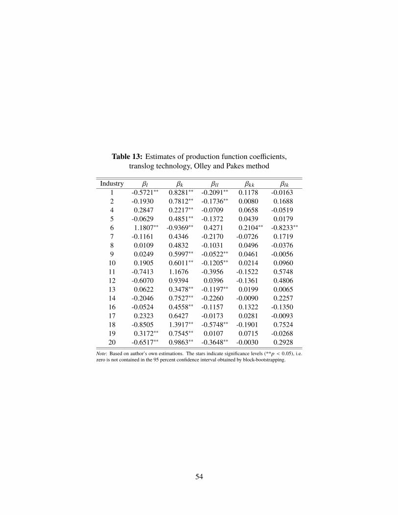
Table 13: Estimates of production function coefficients,translog technology, Olley and Pakes method

Industry βl βk βll βkk βlk1 -0.5721∗∗ 0.8281∗∗ -0.2091∗∗ 0.1178 -0.01632 -0.1930 0.7812∗∗ -0.1736∗∗ 0.0080 0.16884 0.2847 0.2217∗∗ -0.0709 0.0658 -0.05195 -0.0629 0.4851∗∗ -0.1372 0.0439 0.01796 1.1807∗∗ -0.9369∗∗ 0.4271 0.2104∗∗ -0.8233∗∗7 -0.1161 0.4346 -0.2170 -0.0726 0.17198 0.0109 0.4832 -0.1031 0.0496 -0.03769 0.0249 0.5997∗∗ -0.0522∗∗ 0.0461 -0.005610 0.1905 0.6011∗∗ -0.1205∗∗ 0.0214 0.096011 -0.7413 1.1676 -0.3956 -0.1522 0.574812 -0.6070 0.9394 0.0396 -0.1361 0.480613 0.0622 0.3478∗∗ -0.1197∗∗ 0.0199 0.006514 -0.2046 0.7527∗∗ -0.2260 -0.0090 0.225716 -0.0524 0.4558∗∗ -0.1157 0.1322 -0.135017 0.2323 0.6427 -0.0173 0.0281 -0.009318 -0.8505 1.3917∗∗ -0.5748∗∗ -0.1901 0.752419 0.3172∗∗ 0.7545∗∗ 0.0107 0.0715 -0.026820 -0.6517∗∗ 0.9863∗∗ -0.3648∗∗ -0.0030 0.2928

Note: Based on author’s own estimations. The stars indicate significance levels (**p < 0.05), i.e.zero is not contained in the 95 percent confidence interval obtained by block-bootstrapping.

54

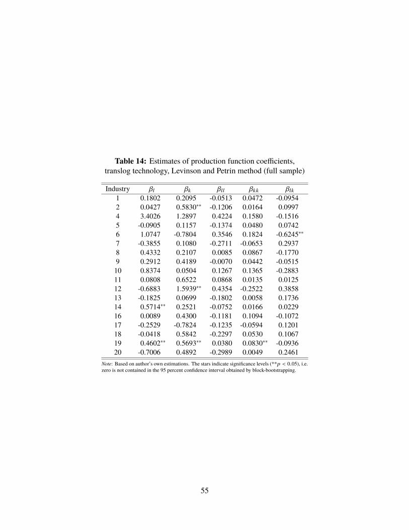
Table 14: Estimates of production function coefficients,translog technology, Levinson and Petrin method (full sample)

Industry βl βk βll βkk βlk1 0.1802 0.2095 -0.0513 0.0472 -0.09542 0.0427 0.5830∗∗ -0.1206 0.0164 0.09974 3.4026 1.2897 0.4224 0.1580 -0.15165 -0.0905 0.1157 -0.1374 0.0480 0.07426 1.0747 -0.7804 0.3546 0.1824 -0.6245∗∗7 -0.3855 0.1080 -0.2711 -0.0653 0.29378 0.4332 0.2107 0.0085 0.0867 -0.17709 0.2912 0.4189 -0.0070 0.0442 -0.051510 0.8374 0.0504 0.1267 0.1365 -0.288311 0.0808 0.6522 0.0868 0.0135 0.012512 -0.6883 1.5939∗∗ 0.4354 -0.2522 0.385813 -0.1825 0.0699 -0.1802 0.0058 0.173614 0.5714∗∗ 0.2521 -0.0752 0.0166 0.022916 0.0089 0.4300 -0.1181 0.1094 -0.107217 -0.2529 -0.7824 -0.1235 -0.0594 0.120118 -0.0418 0.5842 -0.2297 0.0530 0.106719 0.4602∗∗ 0.5693∗∗ 0.0380 0.0830∗∗ -0.093620 -0.7006 0.4892 -0.2989 0.0049 0.2461

Note: Based on author’s own estimations. The stars indicate significance levels (**p < 0.05), i.e.zero is not contained in the 95 percent confidence interval obtained by block-bootstrapping.

55

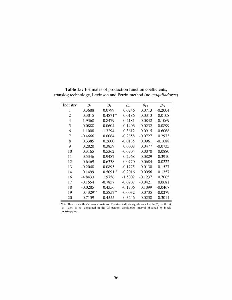
Table 15: Estimates of production function coefficients,translog technology, Levinson and Petrin method (no maquiladoras)

Industry βl βk βll βkk βlk1 0.3688 0.0799 0.0246 0.0713 -0.20042 0.3015 0.4871∗∗ 0.0186 0.0313 -0.01084 1.9368 0.8479 0.2181 0.0842 -0.10695 -0.0888 0.0604 -0.1406 0.0232 0.08996 1.1008 -1.3294 0.3612 0.0915 -0.60687 -0.4666 0.0064 -0.2858 -0.0727 0.29738 0.3385 0.2600 -0.0135 0.0961 -0.16889 0.2820 0.3859 0.0008 0.0477 -0.073510 0.3165 0.5362 -0.0904 0.0070 0.088011 -0.5346 0.9487 -0.2968 -0.0829 0.391012 0.6469 0.6338 0.0770 -0.0684 0.022213 -0.2048 0.0895 -0.1775 0.0130 0.152714 0.1499 0.5091∗∗ -0.2016 0.0056 0.135716 -4.8433 1.9756 -1.5002 -0.1237 0.706517 -0.1554 -0.7857 -0.0907 -0.0421 0.068118 -0.0285 0.4356 -0.1706 0.1099 -0.046719 0.4329∗∗ 0.5857∗∗ -0.0032 0.0735 -0.027920 -0.7159 0.4555 -0.3246 -0.0238 0.3011

Note: Based on author’s own estimations. The stars indicate significance levels (**p < 0.05),i.e. zero is not contained in the 95 percent confidence interval obtained by block-bootstrapping.

56

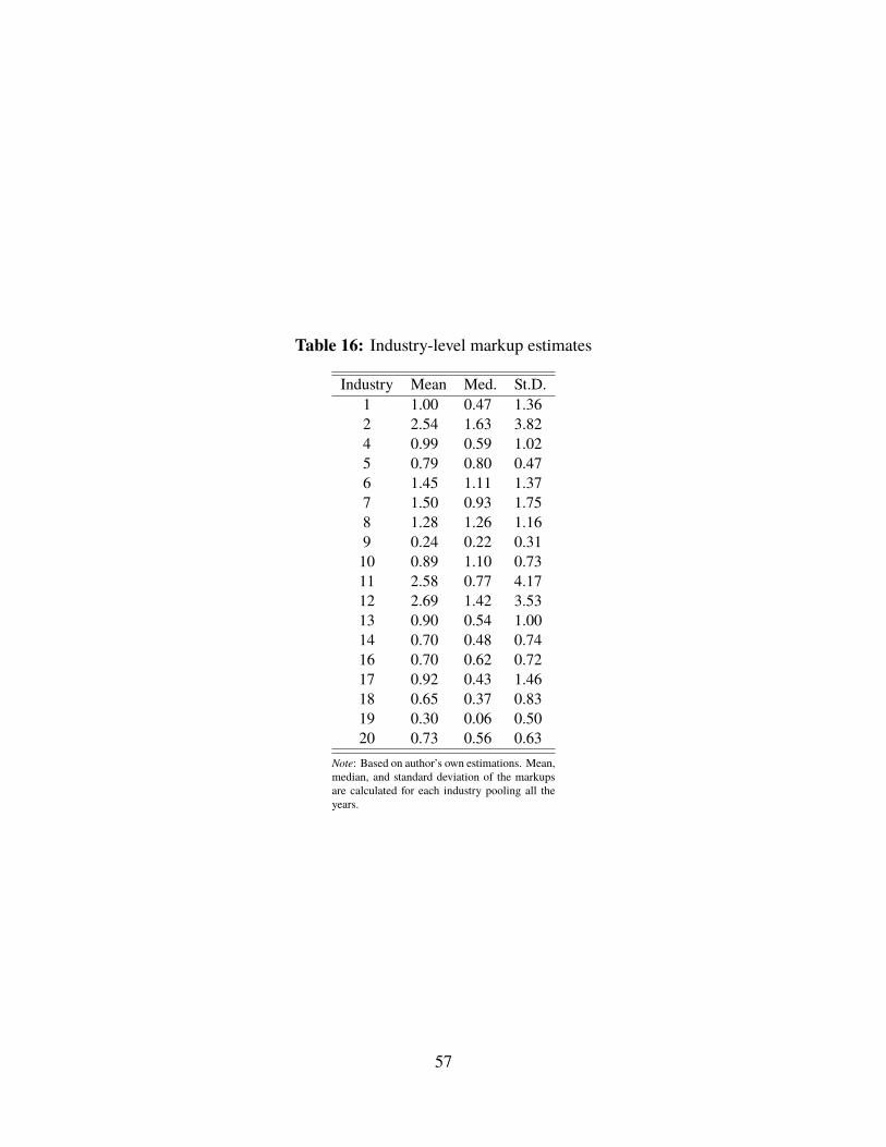
Table 16: Industry-level markup estimates

Industry Mean Med. St.D.1 1.00 0.47 1.362 2.54 1.63 3.824 0.99 0.59 1.025 0.79 0.80 0.476 1.45 1.11 1.377 1.50 0.93 1.758 1.28 1.26 1.169 0.24 0.22 0.3110 0.89 1.10 0.7311 2.58 0.77 4.1712 2.69 1.42 3.5313 0.90 0.54 1.0014 0.70 0.48 0.7416 0.70 0.62 0.7217 0.92 0.43 1.4618 0.65 0.37 0.8319 0.30 0.06 0.5020 0.73 0.56 0.63

Note: Based on author’s own estimations. Mean,median, and standard deviation of the markupsare calculated for each industry pooling all theyears.

57

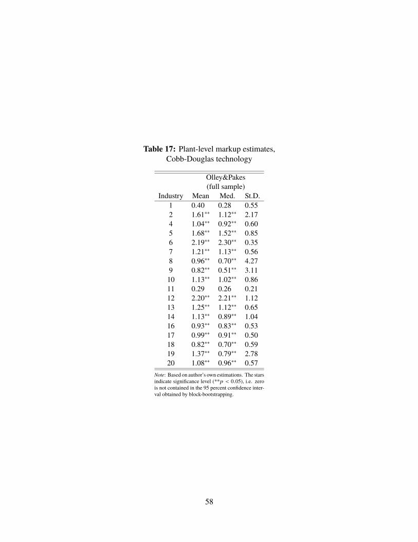
Table 17: Plant-level markup estimates,Cobb-Douglas technology

Olley&Pakes(full sample)

Industry Mean Med. St.D.1 0.40 0.28 0.552 1.61∗∗ 1.12∗∗ 2.174 1.04∗∗ 0.92∗∗ 0.605 1.68∗∗ 1.52∗∗ 0.856 2.19∗∗ 2.30∗∗ 0.357 1.21∗∗ 1.13∗∗ 0.568 0.96∗∗ 0.70∗∗ 4.279 0.82∗∗ 0.51∗∗ 3.1110 1.13∗∗ 1.02∗∗ 0.8611 0.29 0.26 0.2112 2.20∗∗ 2.21∗∗ 1.1213 1.25∗∗ 1.12∗∗ 0.6514 1.13∗∗ 0.89∗∗ 1.0416 0.93∗∗ 0.83∗∗ 0.5317 0.99∗∗ 0.91∗∗ 0.5018 0.82∗∗ 0.70∗∗ 0.5919 1.37∗∗ 0.79∗∗ 2.7820 1.08∗∗ 0.96∗∗ 0.57

Note: Based on author’s own estimations. The starsindicate significance level (**p < 0.05), i.e. zerois not contained in the 95 percent confidence inter-val obtained by block-bootstrapping.

58

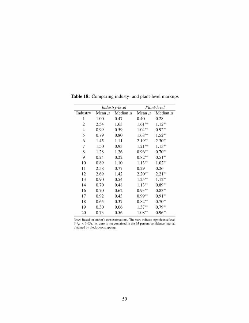
Table 18: Comparing industy- and plant-level markups

Industry-level Plant-levelIndustry Mean µ Median µ Mean µ Median µ

1 1.00 0.47 0.40 0.282 2.54 1.63 1.61∗∗ 1.12∗∗4 0.99 0.59 1.04∗∗ 0.92∗∗5 0.79 0.80 1.68∗∗ 1.52∗∗6 1.45 1.11 2.19∗∗ 2.30∗∗7 1.50 0.93 1.21∗∗ 1.13∗∗8 1.28 1.26 0.96∗∗ 0.70∗∗9 0.24 0.22 0.82∗∗ 0.51∗∗10 0.89 1.10 1.13∗∗ 1.02∗∗11 2.58 0.77 0.29 0.2612 2.69 1.42 2.20∗∗ 2.21∗∗13 0.90 0.54 1.25∗∗ 1.12∗∗14 0.70 0.48 1.13∗∗ 0.89∗∗16 0.70 0.62 0.93∗∗ 0.83∗∗17 0.92 0.43 0.99∗∗ 0.91∗∗18 0.65 0.37 0.82∗∗ 0.70∗∗19 0.30 0.06 1.37∗∗ 0.79∗∗20 0.73 0.56 1.08∗∗ 0.96∗∗

Note: Based on author’s own estimations. The stars indicate significance level(**p < 0.05), i.e. zero is not contained in the 95 percent confidence intervalobtained by block-bootstrapping.

59

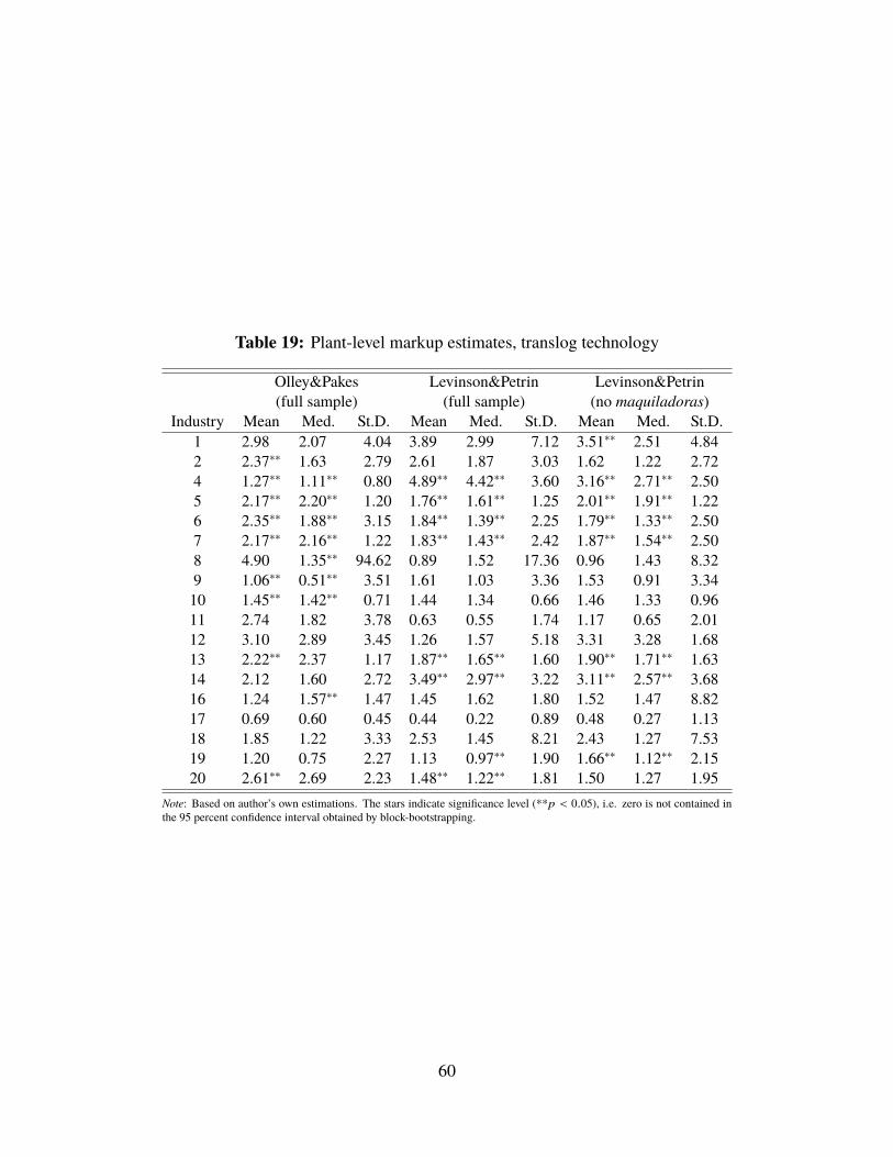
Table 19: Plant-level markup estimates, translog technology

Olley&Pakes Levinson&Petrin Levinson&Petrin(full sample) (full sample) (no maquiladoras)

Industry Mean Med. St.D. Mean Med. St.D. Mean Med. St.D.1 2.98 2.07 4.04 3.89 2.99 7.12 3.51∗∗ 2.51 4.842 2.37∗∗ 1.63 2.79 2.61 1.87 3.03 1.62 1.22 2.724 1.27∗∗ 1.11∗∗ 0.80 4.89∗∗ 4.42∗∗ 3.60 3.16∗∗ 2.71∗∗ 2.505 2.17∗∗ 2.20∗∗ 1.20 1.76∗∗ 1.61∗∗ 1.25 2.01∗∗ 1.91∗∗ 1.226 2.35∗∗ 1.88∗∗ 3.15 1.84∗∗ 1.39∗∗ 2.25 1.79∗∗ 1.33∗∗ 2.507 2.17∗∗ 2.16∗∗ 1.22 1.83∗∗ 1.43∗∗ 2.42 1.87∗∗ 1.54∗∗ 2.508 4.90 1.35∗∗ 94.62 0.89 1.52 17.36 0.96 1.43 8.329 1.06∗∗ 0.51∗∗ 3.51 1.61 1.03 3.36 1.53 0.91 3.3410 1.45∗∗ 1.42∗∗ 0.71 1.44 1.34 0.66 1.46 1.33 0.9611 2.74 1.82 3.78 0.63 0.55 1.74 1.17 0.65 2.0112 3.10 2.89 3.45 1.26 1.57 5.18 3.31 3.28 1.6813 2.22∗∗ 2.37 1.17 1.87∗∗ 1.65∗∗ 1.60 1.90∗∗ 1.71∗∗ 1.6314 2.12 1.60 2.72 3.49∗∗ 2.97∗∗ 3.22 3.11∗∗ 2.57∗∗ 3.6816 1.24 1.57∗∗ 1.47 1.45 1.62 1.80 1.52 1.47 8.8217 0.69 0.60 0.45 0.44 0.22 0.89 0.48 0.27 1.1318 1.85 1.22 3.33 2.53 1.45 8.21 2.43 1.27 7.5319 1.20 0.75 2.27 1.13 0.97∗∗ 1.90 1.66∗∗ 1.12∗∗ 2.1520 2.61∗∗ 2.69 2.23 1.48∗∗ 1.22∗∗ 1.81 1.50 1.27 1.95

Note: Based on author’s own estimations. The stars indicate significance level (**p < 0.05), i.e. zero is not contained inthe 95 percent confidence interval obtained by block-bootstrapping.

60

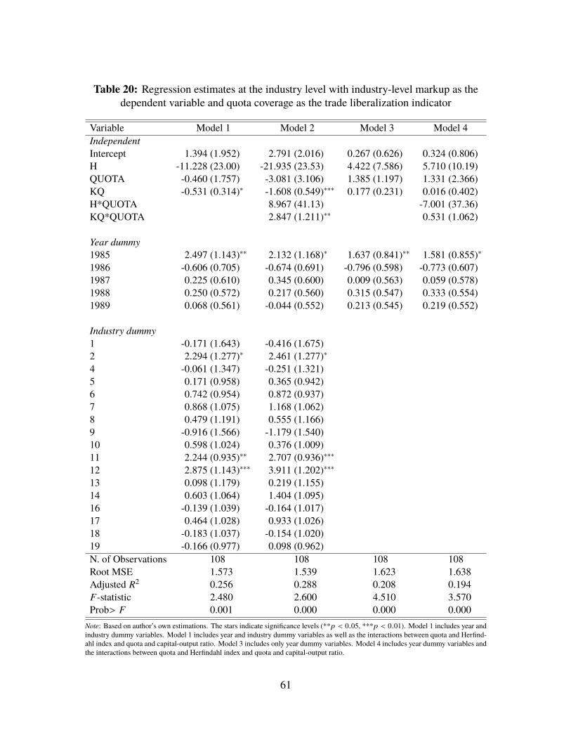
Table 20: Regression estimates at the industry level with industry-level markup as thedependent variable and quota coverage as the trade liberalization indicator

Variable Model 1 Model 2 Model 3 Model 4IndependentIntercept 1.394 (1.952) 2.791 (2.016) 0.267 (0.626) 0.324 (0.806)H -11.228 (23.00) -21.935 (23.53) 4.422 (7.586) 5.710 (10.19)QUOTA -0.460 (1.757) -3.081 (3.106) 1.385 (1.197) 1.331 (2.366)KQ -0.531 (0.314)∗ -1.608 (0.549)∗∗∗ 0.177 (0.231) 0.016 (0.402)H*QUOTA 8.967 (41.13) -7.001 (37.36)KQ*QUOTA 2.847 (1.211)∗∗ 0.531 (1.062)

Year dummy1985 2.497 (1.143)∗∗ 2.132 (1.168)∗ 1.637 (0.841)∗∗ 1.581 (0.855)∗1986 -0.606 (0.705) -0.674 (0.691) -0.796 (0.598) -0.773 (0.607)1987 0.225 (0.610) 0.345 (0.600) 0.009 (0.563) 0.059 (0.578)1988 0.250 (0.572) 0.217 (0.560) 0.315 (0.547) 0.333 (0.554)1989 0.068 (0.561) -0.044 (0.552) 0.213 (0.545) 0.219 (0.552)

Industry dummy1 -0.171 (1.643) -0.416 (1.675)2 2.294 (1.277)∗ 2.461 (1.277)∗4 -0.061 (1.347) -0.251 (1.321)5 0.171 (0.958) 0.365 (0.942)6 0.742 (0.954) 0.872 (0.937)7 0.868 (1.075) 1.168 (1.062)8 0.479 (1.191) 0.555 (1.166)9 -0.916 (1.566) -1.179 (1.540)10 0.598 (1.024) 0.376 (1.009)11 2.244 (0.935)∗∗ 2.707 (0.936)∗∗∗12 2.875 (1.143)∗∗∗ 3.911 (1.202)∗∗∗13 0.098 (1.179) 0.219 (1.155)14 0.603 (1.064) 1.404 (1.095)16 -0.139 (1.039) -0.164 (1.017)17 0.464 (1.028) 0.933 (1.026)18 -0.183 (1.037) -0.154 (1.020)19 -0.166 (0.977) 0.098 (0.962)N. of Observations 108 108 108 108Root MSE 1.573 1.539 1.623 1.638Adjusted R2 0.256 0.288 0.208 0.194F-statistic 2.480 2.600 4.510 3.570Prob> F 0.001 0.000 0.000 0.000

Note: Based on author’s own estimations. The stars indicate significance levels (**p < 0.05, ***p < 0.01). Model 1 includes year andindustry dummy variables. Model 1 includes year and industry dummy variables as well as the interactions between quota and Herfind-ahl index and quota and capital-output ratio. Model 3 includes only year dummy variables. Model 4 includes year dummy variables andthe interactions between quota and Herfindahl index and quota and capital-output ratio.

61

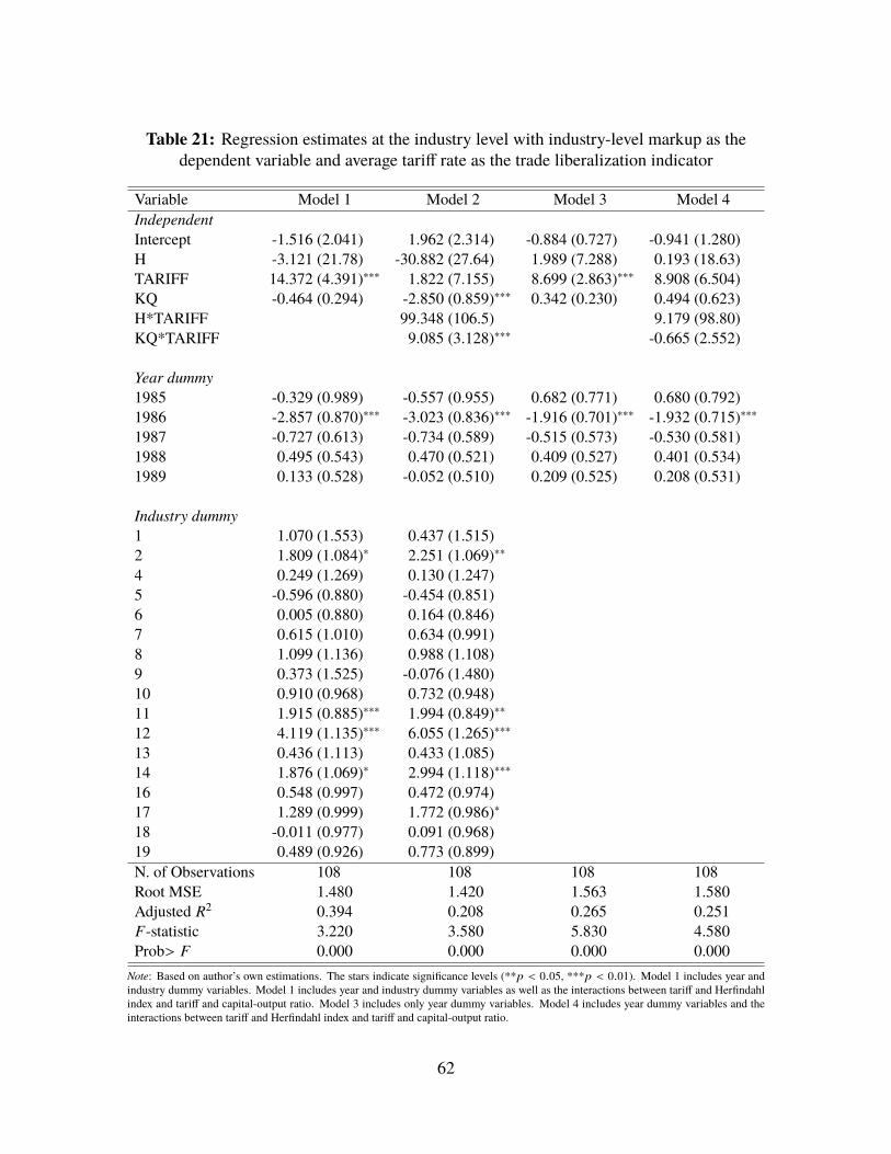
Table 21: Regression estimates at the industry level with industry-level markup as thedependent variable and average tariff rate as the trade liberalization indicator

Variable Model 1 Model 2 Model 3 Model 4IndependentIntercept -1.516 (2.041) 1.962 (2.314) -0.884 (0.727) -0.941 (1.280)H -3.121 (21.78) -30.882 (27.64) 1.989 (7.288) 0.193 (18.63)TARIFF 14.372 (4.391)∗∗∗ 1.822 (7.155) 8.699 (2.863)∗∗∗ 8.908 (6.504)KQ -0.464 (0.294) -2.850 (0.859)∗∗∗ 0.342 (0.230) 0.494 (0.623)H*TARIFF 99.348 (106.5) 9.179 (98.80)KQ*TARIFF 9.085 (3.128)∗∗∗ -0.665 (2.552)

Year dummy1985 -0.329 (0.989) -0.557 (0.955) 0.682 (0.771) 0.680 (0.792)1986 -2.857 (0.870)∗∗∗ -3.023 (0.836)∗∗∗ -1.916 (0.701)∗∗∗ -1.932 (0.715)∗∗∗1987 -0.727 (0.613) -0.734 (0.589) -0.515 (0.573) -0.530 (0.581)1988 0.495 (0.543) 0.470 (0.521) 0.409 (0.527) 0.401 (0.534)1989 0.133 (0.528) -0.052 (0.510) 0.209 (0.525) 0.208 (0.531)

Industry dummy1 1.070 (1.553) 0.437 (1.515)2 1.809 (1.084)∗ 2.251 (1.069)∗∗4 0.249 (1.269) 0.130 (1.247)5 -0.596 (0.880) -0.454 (0.851)6 0.005 (0.880) 0.164 (0.846)7 0.615 (1.010) 0.634 (0.991)8 1.099 (1.136) 0.988 (1.108)9 0.373 (1.525) -0.076 (1.480)10 0.910 (0.968) 0.732 (0.948)11 1.915 (0.885)∗∗∗ 1.994 (0.849)∗∗12 4.119 (1.135)∗∗∗ 6.055 (1.265)∗∗∗13 0.436 (1.113) 0.433 (1.085)14 1.876 (1.069)∗ 2.994 (1.118)∗∗∗16 0.548 (0.997) 0.472 (0.974)17 1.289 (0.999) 1.772 (0.986)∗18 -0.011 (0.977) 0.091 (0.968)19 0.489 (0.926) 0.773 (0.899)N. of Observations 108 108 108 108Root MSE 1.480 1.420 1.563 1.580Adjusted R2 0.394 0.208 0.265 0.251F-statistic 3.220 3.580 5.830 4.580Prob> F 0.000 0.000 0.000 0.000

Note: Based on author’s own estimations. The stars indicate significance levels (**p < 0.05, ***p < 0.01). Model 1 includes year andindustry dummy variables. Model 1 includes year and industry dummy variables as well as the interactions between tariff and Herfindahlindex and tariff and capital-output ratio. Model 3 includes only year dummy variables. Model 4 includes year dummy variables and theinteractions between tariff and Herfindahl index and tariff and capital-output ratio.

62

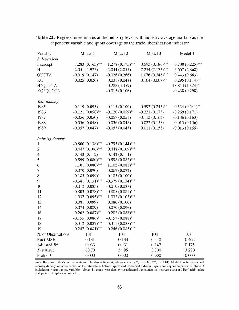
Table 22: Regression estimates at the industry level with industry-average markup as thedependent variable and quota coverage as the trade liberalization indicator

Variable Model 1 Model 2 Model 3 Model 4IndependentIntercept 1.283 (0.163)∗∗∗ 1.278 (0.175)∗∗∗ 0.593 (0.180)∗∗∗ 0.700 (0.225)∗∗∗H -2.051 (1.923) -2.044 (2.055) 7.254 (2.173)∗∗∗ 3.667 (2.868)QUOTA -0.019 (0.147) -0.026 (0.266) 1.076 (0.346)∗∗∗ 0.443 (0.663)KQ 0.025 (0.026) 0.031 (0.048) 0.164 (0.067)∗∗ 0.295 (0.114)∗∗H*QUOTA 0.288 (3.459) 18.843 (10.24)∗KQ*QUOTA -0.015 (0.106) -0.438 (0.298)

Year dummy1985 -0.119 (0.095) -0.115 (0.100) -0.593 (0.243)∗∗ -0.534 (0.241)∗∗1986 -0.121 (0.058)∗∗ -0.120 (0.059)∗∗ -0.231 (0.173) -0.269 (0.171)1987 -0.056 (0.050) -0.057 (0.051) -0.113 (0.163) -0.186 (0.163)1988 -0.036 (0.048) -0.036 (0.048) 0.022 (0.158) -0.013 (0.156)1989 -0.057 (0.047) -0.057 (0.047) 0.011 (0.158) -0.013 (0.155)

Industry dummy1 -0.800 (0.138)∗∗∗ -0.795 (0.144)∗∗∗2 0.447 (0.106)∗∗∗ 0.448 (0.109)∗∗∗4 -0.143 (0.112) -0.142 (0.114)5 0.599 (0.080)∗∗∗ 0.598 (0.082)∗∗∗6 1.101 (0.080)∗∗∗ 1.102 (0.081)∗∗∗7 0.070 (0.090) 0.069 (0.092)8 -0.183 (0.099)∗ -0.183 (0.100)∗9 -0.381 (0.131)∗∗∗ -0.379 (0.134)∗∗∗10 -0.012 (0.085) -0.010 (0.087)11 -0.803 (0.078)∗∗∗ -0.805 (0.081)∗∗∗12 1.037 (0.095)∗∗∗ 1.032 (0.103)∗∗∗13 0.081 (0.099) 0.080 (0.100)14 0.074 (0.089) 0.070 (0.096)16 -0.202 (0.087)∗∗ -0.202 (0.088)∗∗∗17 -0.155 (0.086)∗ -0.157 (0.088)∗18 -0.312 (0.087)∗∗∗ -0.311 (0.088)∗∗∗19 0.247 (0.081)∗∗∗ 0.246 (0.083)∗∗∗N. of Observations 108 108 108 108Root MSE 0.131 0.133 0.470 0.462Adjusted R2 0.933 0.931 0.147 0.175F-statistic 60.70 54.85 3.300 3.280Prob> F 0.000 0.000 0.000 0.000

Note: Based on author’s own estimations. The stars indicate significance levels (**p < 0.05, ***p < 0.01). Model 1 includes year andindustry dummy variables as well as the interactions between quota and Herfindahl index and quota and capital-output ratio. Model 3includes only year dummy variables. Model 4 includes year dummy variables and the interactions between quota and Herfindahl indexand quota and capital-output ratio.

63

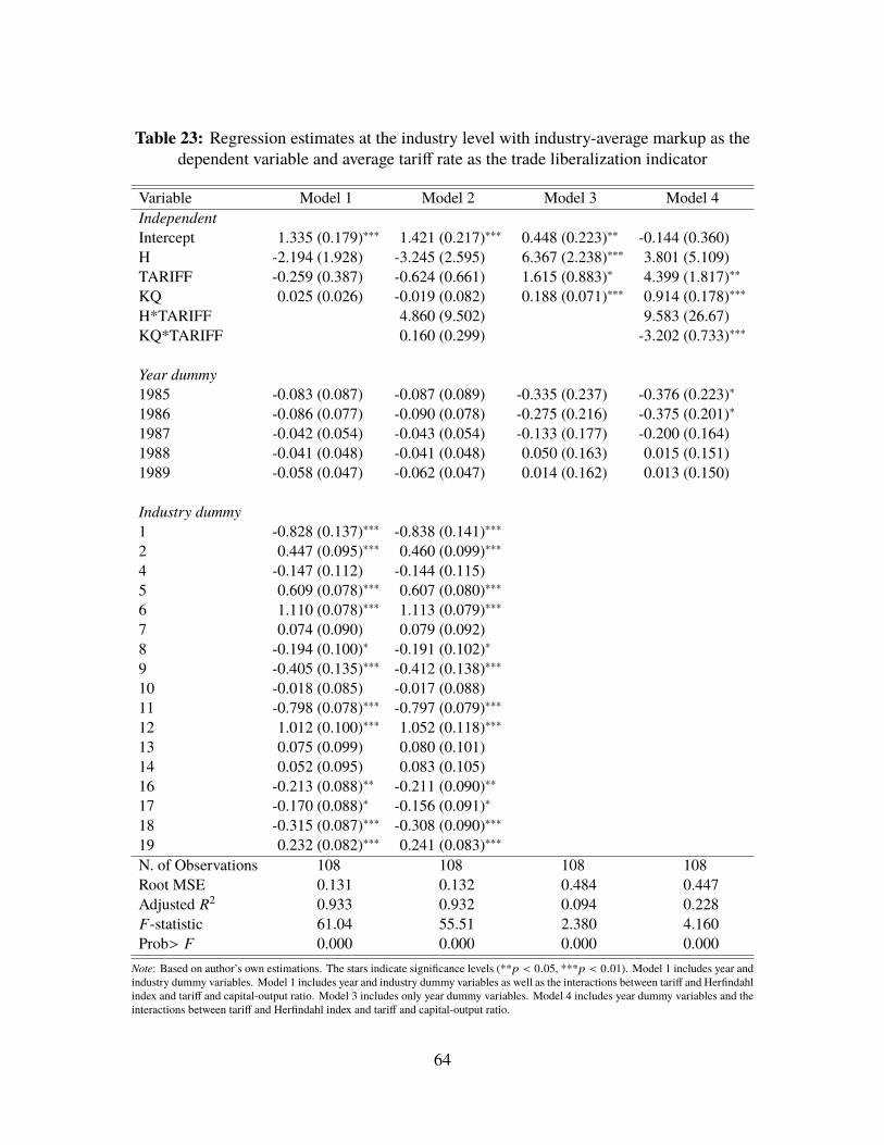
Table 23: Regression estimates at the industry level with industry-average markup as thedependent variable and average tariff rate as the trade liberalization indicator

Variable Model 1 Model 2 Model 3 Model 4IndependentIntercept 1.335 (0.179)∗∗∗ 1.421 (0.217)∗∗∗ 0.448 (0.223)∗∗ -0.144 (0.360)H -2.194 (1.928) -3.245 (2.595) 6.367 (2.238)∗∗∗ 3.801 (5.109)TARIFF -0.259 (0.387) -0.624 (0.661) 1.615 (0.883)∗ 4.399 (1.817)∗∗KQ 0.025 (0.026) -0.019 (0.082) 0.188 (0.071)∗∗∗ 0.914 (0.178)∗∗∗H*TARIFF 4.860 (9.502) 9.583 (26.67)KQ*TARIFF 0.160 (0.299) -3.202 (0.733)∗∗∗

Year dummy1985 -0.083 (0.087) -0.087 (0.089) -0.335 (0.237) -0.376 (0.223)∗1986 -0.086 (0.077) -0.090 (0.078) -0.275 (0.216) -0.375 (0.201)∗1987 -0.042 (0.054) -0.043 (0.054) -0.133 (0.177) -0.200 (0.164)1988 -0.041 (0.048) -0.041 (0.048) 0.050 (0.163) 0.015 (0.151)1989 -0.058 (0.047) -0.062 (0.047) 0.014 (0.162) 0.013 (0.150)

Industry dummy1 -0.828 (0.137)∗∗∗ -0.838 (0.141)∗∗∗2 0.447 (0.095)∗∗∗ 0.460 (0.099)∗∗∗4 -0.147 (0.112) -0.144 (0.115)5 0.609 (0.078)∗∗∗ 0.607 (0.080)∗∗∗6 1.110 (0.078)∗∗∗ 1.113 (0.079)∗∗∗7 0.074 (0.090) 0.079 (0.092)8 -0.194 (0.100)∗ -0.191 (0.102)∗9 -0.405 (0.135)∗∗∗ -0.412 (0.138)∗∗∗10 -0.018 (0.085) -0.017 (0.088)11 -0.798 (0.078)∗∗∗ -0.797 (0.079)∗∗∗12 1.012 (0.100)∗∗∗ 1.052 (0.118)∗∗∗13 0.075 (0.099) 0.080 (0.101)14 0.052 (0.095) 0.083 (0.105)16 -0.213 (0.088)∗∗ -0.211 (0.090)∗∗17 -0.170 (0.088)∗ -0.156 (0.091)∗18 -0.315 (0.087)∗∗∗ -0.308 (0.090)∗∗∗19 0.232 (0.082)∗∗∗ 0.241 (0.083)∗∗∗N. of Observations 108 108 108 108Root MSE 0.131 0.132 0.484 0.447Adjusted R2 0.933 0.932 0.094 0.228F-statistic 61.04 55.51 2.380 4.160Prob> F 0.000 0.000 0.000 0.000

Note: Based on author’s own estimations. The stars indicate significance levels (**p < 0.05, ***p < 0.01). Model 1 includes year andindustry dummy variables. Model 1 includes year and industry dummy variables as well as the interactions between tariff and Herfindahlindex and tariff and capital-output ratio. Model 3 includes only year dummy variables. Model 4 includes year dummy variables and theinteractions between tariff and Herfindahl index and tariff and capital-output ratio.

64

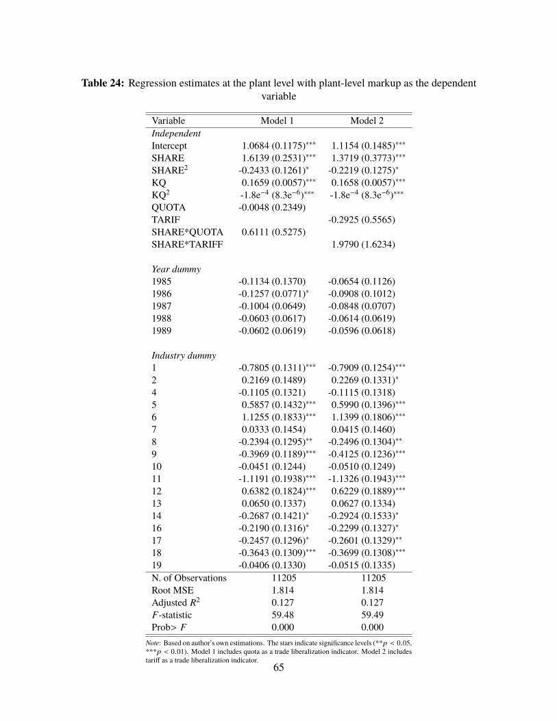
Table 24: Regression estimates at the plant level with plant-level markup as the dependentvariable

Variable Model 1 Model 2IndependentIntercept 1.0684 (0.1175)∗∗∗ 1.1154 (0.1485)∗∗∗SHARE 1.6139 (0.2531)∗∗∗ 1.3719 (0.3773)∗∗∗SHARE2 -0.2433 (0.1261)∗ -0.2219 (0.1275)∗KQ 0.1659 (0.0057)∗∗∗ 0.1658 (0.0057)∗∗∗KQ2 -1.8e−4 (8.3e−6)∗∗∗ -1.8e−4 (8.3e−6)∗∗∗QUOTA -0.0048 (0.2349)TARIF -0.2925 (0.5565)SHARE*QUOTA 0.6111 (0.5275)SHARE*TARIFF 1.9790 (1.6234)

Year dummy1985 -0.1134 (0.1370) -0.0654 (0.1126)1986 -0.1257 (0.0771)∗ -0.0908 (0.1012)1987 -0.1004 (0.0649) -0.0848 (0.0707)1988 -0.0603 (0.0617) -0.0614 (0.0619)1989 -0.0602 (0.0619) -0.0596 (0.0618)

Industry dummy1 -0.7805 (0.1311)∗∗∗ -0.7909 (0.1254)∗∗∗2 0.2169 (0.1489) 0.2269 (0.1331)∗4 -0.1105 (0.1321) -0.1115 (0.1318)5 0.5857 (0.1432)∗∗∗ 0.5990 (0.1396)∗∗∗6 1.1255 (0.1833)∗∗∗ 1.1399 (0.1806)∗∗∗7 0.0333 (0.1454) 0.0415 (0.1460)8 -0.2394 (0.1295)∗∗ -0.2496 (0.1304)∗∗9 -0.3969 (0.1189)∗∗∗ -0.4125 (0.1236)∗∗∗10 -0.0451 (0.1244) -0.0510 (0.1249)11 -1.1191 (0.1938)∗∗∗ -1.1326 (0.1943)∗∗∗12 0.6382 (0.1824)∗∗∗ 0.6229 (0.1889)∗∗∗13 0.0650 (0.1337) 0.0627 (0.1334)14 -0.2687 (0.1421)∗ -0.2924 (0.1533)∗16 -0.2190 (0.1316)∗ -0.2299 (0.1327)∗17 -0.2457 (0.1296)∗ -0.2601 (0.1329)∗∗18 -0.3643 (0.1309)∗∗∗ -0.3699 (0.1308)∗∗∗19 -0.0406 (0.1330) -0.0515 (0.1335)N. of Observations 11205 11205Root MSE 1.814 1.814Adjusted R2 0.127 0.127F-statistic 59.48 59.49Prob> F 0.000 0.000

Note: Based on author’s own estimations. The stars indicate significance levels (**p < 0.05,***p < 0.01). Model 1 includes quota as a trade liberalization indicator. Model 2 includestariff as a trade liberalization indicator.

65

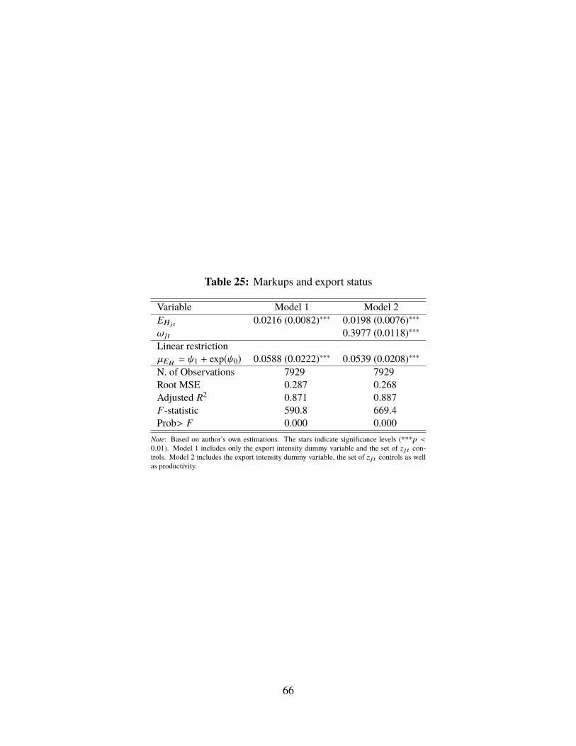
Table 25: Markups and export status

Variable Model 1 Model 2EHj t 0.0216 (0.0082)∗∗∗ 0.0198 (0.0076)∗∗∗ωjt 0.3977 (0.0118)∗∗∗Linear restrictionµEH = ψ1 + exp(ψ0) 0.0588 (0.0222)∗∗∗ 0.0539 (0.0208)∗∗∗N. of Observations 7929 7929Root MSE 0.287 0.268Adjusted R2 0.871 0.887F-statistic 590.8 669.4Prob> F 0.000 0.000

Note: Based on author’s own estimations. The stars indicate significance levels (***p <0.01). Model 1 includes only the export intensity dummy variable and the set of z j t con-trols. Model 2 includes the export intensity dummy variable, the set of z j t controls as wellas productivity.

66