planned lead times in multistage systems

Decision Sciences Volume 29 Number I Winter 1998 Printed in the U.S.A.

Planned Lead Times in Multistage Systems Ram P. Mohan Adapta Solutions, Inc., 22 Saw Mill River Road, Hawthorne, NY 10532, email: ram-mohan @adaptasolutions.com

Larry P. Ritzman Operations and Strategic Management, Boston College, Chestnut Hill, MA 021 67, email: ritzman @ bc.edu

ABSTRACT This study investigates the impact of planned lead times on performance in multistage manufacturing where material requirements planning is used in a make-to-stock environment. We simulate a variety of different operating environments and find: (1) planned lead times are important to customer service levels under all operating environments examined, but have a smaller impact on inventory investment; (2) tight due dates introduced by short planned lead times hurt customer service without saving much inventory; (3) small increases to tight planned lead times improve customer service substantially with small inventory increases; (4) co-component inventories change with planned lead times, and disparity between such inventories is a sign of poor timing coordination; (5) the fixed order quantity rule performs better than the periodic order quantity rule; and (6) tall product structure and large lot sizes require particular attention to planned lead times. The findings also extend the current understanding of planned lead times by including uncertainties such as forecast error, yield loss, and equipment reliability. The study concludes with a way to diagnose and improve poorly set planned lead times.

Subject Areas: Inventory Management, Material Requirements Planning, Pro- duction and Inventory Control Systems, and Simulation.

INTRODUCTION Multistage production is a fact of life for most manufacturers. Regardless of the production and inventory control system, the objective is to provide good customer service with low inventory levels. Control systems achieve this objective through a coordinated component production that supplies the right quantity at the right time. This research uses material requirements planning (MRP) as the control system in a make-to-stock environment. MRP is used because surveys by Anderson, Schroeder, Tupy, and White (1982), LaForge and Sturr (1986), and Sharma (1987) showed that the MRP system is still the workhorse in U.S. manufacturing organi- zations. Further, it was shown in Krajewski, King, Ritzman, and Wong (1987) that

163

164 Planned Lead Times in Multistage Systems

MRP performs much like a kanban system in manufacturing environments for which JIT is intended.

There are two procedures in MRP that help in coordinating component production. First, using a parent’s order schedule in deriving gross requirements of all its components helps in coordinating co-component demand. These gross requirements are used in determining production order quantities. Second, these production orders are offset by component lead time estimates called planned lead times (PLTs). When PLTs are larger than actual lead times, inventories increase because components are produced before they are needed; smaller PLTs cause component nonavailability and delay in assembling parents. Therefore, PLTs should be set properly to facilitate coordinated production timing.

Though there has been considerable lot-sizing research on multistage production systems, there has been much less attention given to the timing issue. MRP pioneers offer different views on PLT importance and desired values. Orlicky (1975) stated that the disparity between planned and actual lead times is “of no concern” (p. 83), and “the old concept of an accurate planned lead time must be discarded” (p. 261). Plossl and Welch (1979) emphasized that PLTs must be as small as possible. On the other hand, there are also advantages and disadvantages to large PLTs. Large PLTs help in increased component availability, parent’s timely production, and improved customer service. Large PLTs increase inventory and require a longer planning horizon, introducing a greater degree of uncertainty. Higher uncertainty can affect inventory levels and customer service, and nullify the benefits of a parent’s timely production.

Planned lead times are enigmatic in that there are arguments supporting every possible view: PLTs do not significantly affect manufacturing performance, they should be large, or they should be as small as possible. Even among the few studies on PLTs, there are contradictions indicating a need for better understanding. Efforts such as analyzing and simplifying the production process to minimize the manufacturing lead time, as done in time-based competition, can be critical to an organization’s success. Whether or not such efforts are undertaken, companies still must decide on appropriate PLTs. This study focuses on whether PLTs should be small or large relative to manufacturing lead time.

Literature Review Whybark and William (1976), while comparing the buffering alternatives of safety stock and safety lead time, concluded that safety stock better copes with quantity uncertainty, while safety lead time better copes with timing uncertainty. Grasso and Taylor (1984) studied the impact of supply-timing uncertainties on manufacturing performance, but they found that safety stock copes better with supply- timing uncertainty than does safety lead time.

Melnyk and Piper (1985) examined the impact of lot-sizing rules on “lead- time errors” (the difference between an item’s PLT and its average manufacturing lead time) and the impact of PLT magnitude on manufacturing performance. They found that larger PLTs improve on-time end item deliveries, and that dynamic lot- sizing rules are better than static lot-sizing rules with smaller lead-time errors, lower inventory levels, and higher on-time end item deliveries.

Mohan and Ritzman 165

St. John (1985) found that larger PLTs increase cost and supports the view that PLTs must be as small as possible. In particular, the carrying cost-applied to raw materials, work in process, and finished goods inventory-contributes most to this cost increase. In contrast, Marlin ( 1986) suggested that inventory levels increase with the lead-time error magnitude rather than with the PLT magnitude. As PLTs are increased, the inventory levels first decrease (when PLTs are less than the average manufacturing lead time), and then increase after reaching a minimum level. Marlin stated that the decrease-increase in inventory “contradicts the finding of St. John, in which inventory (storeroom plus WIP) was found to increase over all values of lead time slack’ (p. 191). Marlin explained that this contradiction is due to shortcomings in the simulator used in St. John’s study. Kanet (1986) also provided an explanation supporting Marlin’s decrease-increase inventory behavior. Penlesky, Berry, and Wemmerlov (1989), while focusing on open order due date adjustments, concluded that customer service improves with larger PLTs, but inventory behaves in a mixed manner.

In addition to these empirical investigations on PLTs, Weeks (1978), Kanet (1986), Yano (1987a, 1987b, 1987c) and Hoyt (1978) have investigated ways to prescribe PLTs. Weeks proposed a one-period inventory model to set the optimal PLT and suggested that the PLT is a function of the cost of lateness, earliness, due date length, and the manufacturing lead-time distribution. Kanet recommended PLTs in which allowances are set proportional to total work content. Yano suggested a nonlinear optimizing model, assuming that the lead-time distribution of all items in a bill of material (BOM) is known. Hoyt suggested the QUOAT method, based on simple queuing models, for setting PLTs.

Issues and Objectives in This Study There are at least four issues that remain to be addressed. First, the impact of PLTs on inventory seems inconclusive and contradictory. The “decrease-increase” pattern suggested by Kanet (1986) and Marlin (1986) directs future research towards determining the PLT that minimizes inventories. PLTs smaller than such inventory minimizing PLTs are a lose-lose situation: higher cost and poorer customer service. The “continually increasing inventory” pattern suggested by St. John ( 1985) implies that gaining in one dimension means losing in another dimension.

Second, some past research, such as in Melnyk and Piper (1983, was conducted before the impact of small and large lot sizes was well documented. Con- sequently, lot-size magnitude and lot-sizing rule factors are inadvertently confounded in the experimental design. For example, using lot-for-lot and fixed order quantity rules (with average lot size greater than one period’s average demand) confounds the two factors. The choice between static and dynamic lot- sizing rules needs to be revisited when the two factors are carefully controlled.

Third, none of the above-mentioned research uses product structure as an experimental factor. Do product structures with more components per item, or those with more manufacturing stages, require a greater degree of coordinated component production‘? Finally, all the previous research included only demand uncertainty but excluded yield loss uncertainty and equipment reliability. Do the results in past research extend when these additional uncertainties are included?


This study addresses these four issues. Lot-size magnitude is carefully controlled, product structures are a separate experimental factor, and a full range of uncertainties is included. A fundamental objective is to determine whether PLTs are an important factor requiring careful managerial consideration, or whether the disparity between planned and actual lead times is “of no concern.” A corollary to this objective is whether this importance is contingent on factors such as the type of product structure. Finally, this study proposes a new diagnostic measure that identifies poorly set PLTs and provides guidelines to improve these settings.

In investigating these four issues, our approach is to make the environmental settings as realistic as possible. The advantage to this is that our results may be more easily applied to environments for which they are intended, rather than developing solutions to simple situations that do not exist in practice. Ritzman and King (1993), Malhotra and Ritzman (1990), and Krajewski et al. (1987) set prece- dents to this kind of research approach, and they addressed a wide range of issues in production and inventory control. To achieve realism, we were guided by two sources. First, Krajewski et al. was selected because their settings were guided by a panel of managers from a variety of manufacturing plants across the United States. These managers believed that the high and low settings bracketed the range of reasonable possibilities across a wide variety of factors. We selected the mid- point between the low and high settings for many of the shop and product factors so as to have representative values for them. Second, we used the data from Sharma’s (1987) empirical study to guide us in setting factors such as average yield, and mean time between failures. We also explored both low and high settings for a few factors, ones that we believed could be critical to choosing the best strategy for planned lead times. These factors, along with the planned lead times themselves, are identified as experimental factors in the research methodology section.

Performance Measures We monitor two manufacturing performance measures. The first is the total average inventory investment, expressed in days of supply. This measure is the average time-integrated dollar value of inventory divided by the average dollar demand per day of end items. Inventory includes stockroom and work-in-process inventories of all produced items. The second measure is customer service, expressed in days of past due. This measure is the average time-integrated dollar value of back- orders, divided by the average dollar demand per day of end items. The days of past due measure quantifies the delay in satisfying customer orders and does not have a limited range of values unlike fill-rate percentages. A wide range of factor levels can result in fill rates clustering around 0 and loo%, and such clustering reduces the ability to distinguish between differences in actual performances.

The next section describes the experimental factors, fixed factors, simulation model, and data gathering included in this study. The third section presents the research hypotheses formally, and the fourth and fifth sections discuss the results. The final section concludes with a summary of findings and suggestions for future research.

Mohan and Ritunan 167

RESEARCH METHODOLOGY This study includes six experimental factors summarized in Table 1 and more fully described below.

Planned Lead Times An item’s manufacturing lead time has three constituents: order processing time that includes setup time and processing time for all units in the order, queuing time resulting from limited capacity, and component delay resulting from component unavailability. The complex relationship between a parent’s component delay and its component PLT, queuing time variability, and order processing time variability due to lot size variability make PLT setting a complex decision. Finally, equating an item’s PLT to its average manufacturing lead time may not be the best alternative because such PLTs ignore the impact of lead-time variability.

Given our focus on planned lead times, this factor has four levels: low, medium-low, medium-high, and high. All four levels set the PLTs equal to the average order processing time plus a multiplier times the sum of the average queue time and component delay. This multiplier varies from 0.25 through 1 .OO, in incre- ments of 0.25. These factor settings avoid PLTs less than the average order processing time, as such PLTs are undesirable (Ragatz, 1989). Multipliers beyond 1.00 such as 1.25, tested on a few experimental cells, did not provide any additional managerially significant insights. Such large PLTs provided zero days of past due customer service and very high inventory levels.

Product Structure The product structure, which specifies parent-component relationships, can be characterized by the number of items, the number of levels, the average number of components per parent, and the average number of parents per component. Researchers such as Blackbum and Millen (1982), Bott and Ritzman (1983), Ritzman and Krajewski (1983), Benton and Srivastava (1985), and Fry, Oliff, Minor, and Leong (1989), considered the number of levels as a key product structure charac- teristic. This factor, however, has not been included in previous PLT research. Including product structure as an experimental factor helps identify which product structure requires a more careful timing coordination: more levels or more components per parent.

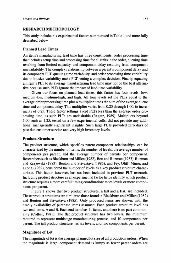
Figure 1 shows that two product structures, a tall and a flat, are included. These product structures are similar to those found in Blackburn and Millen (1982) and Benton and Srivastava (1985). Only produced items are shown, with the timely availability of purchase items assumed. Each product structure level has two end items, A and B. Each end item has 11 items, and there is no part commonality (Collier, 1981). The flat product structure has two levels, the minimum required to represent multistage manufacturing process, and 10 components per parent. The tall product structure has six levels, and two components per parent.

Magnitude of Lot The magnitude of lot is the average planned lot size of all production orders. When the magnitude is large, component demand is lumpy as fewer parent orders are

I68 Plmned Lead Times in Multistage Systems

Table 1: Summary of experimental factors.

Experimental Factors Factor Level Description 1. Planned Lead Time

Low Medium-low Medium-high High

2. Product Structure Low High

3. Magnitude of Lot Low High

4. Lot-Sizing Rules Low High

5. Shop Capacity Utilization Low High

6. Degree of Dominance Low

High

Order run time + 0.25 (queue time + component delay) Order run time t 0.50 (queue time + component delay) Order run time + 0.75 (queue time + component delay) Order run time + 1 .OO (queue time + component delay)

Flat, with two levels in the BOM Tall. with six levels in the BOM

5 days of supply 20 days of supply

Fixed order quantity (FOQ) Periodic order quantity (POQ)

80% 90%

Equal average order run times for items processed in a department. Unequal average order processing times for items processed in a department.

released. Such lumpy demand creates workload surges and increases queuing time variability. Krajewski et al. (1987) and Penlesky et al. (1989) found that this factor is an important determinant of manufacturing performance. Further, Karmarkar (1 987) suggested that average queuing time and magnitude of lot have a nonlinear relationship in a capacitated environment. Thus, magnitude of lot can have a direct impact on manufacturing performance, and an indirect effect through its impact on manufacturing lead time. Japanese manufacturing companies’ superior performance is often attributed to small lot sizes. As with product structure, this factor is not included in previous PLT studies.

In this study, five days of supply represents a small magnitude and 20 days of supply a large magnitude. The lot size is held at the same level for both end and intermediate items. These selections are similar to the selections in Krajewski et al. (1987) and Penlesky et al. (1989). Further, Sharma’s (1987) study reported that the magnitude of lot was no more than five days of supply in 36% of the companies surveyed, while 46% of the companies had no less than 20 days of supply.

Mohan and Ritunun 169

Figure 1: Flat and tall product structures.

a. Tall Product Structure

b. Flat Product Structure

Note: All usage quantities are one, and purchased items are not shown.

Lot-Sizing Rules Lot-sizing rules have received considerable attention in past research as suggested by the surveys of Bahl, Ritzman, and Gupta (1987), and by statistics in Amoako- Gyampah and Meredith (1989). This factor is included because lot-sizing rules have been shown to be a significant factor affecting PLT decision (Melnyk 8z Piper, 1985).

The lot-sizing rule factor in this study has two contrasting levels: fixed order quantity (FOQ), representing the static lot-sizing rules, and periodic order quantity (POQ), representing the dynamic lot-sizing rules. The FOQ rule specifies order quantities that are insensitive to the demand characteristics and do not vary from order to order. As requirements change, the time between orders change. The POQ rule alters order quantities to fit the demand pattern.


Shop Capacity Utilization Production is achieved through operators working on machines. Each operator is assigned to a department and is trained to work on all machines in the department. Operators are the limiting resource because there are more machines than operators in each department. The shop capacity utilization is the mean of the average department utilizations. A department’s utilization equals the average of all operator utilizations in the department. An operator’s utilization, expressed in percentage, equals utilized time divided by available time. An operator’s utilized time includes setting up machines, processing individual units in orders, and repairing machines when they fail. PLT studies indicate that capacity utilization is an important factor significantly affecting manufacturing performance (Marlin 1986; Penlesky et al., 1989).

Two factor levels are included: an 80% and a 90% average utilization. These levels are identical to those in Marlin (1986). Further, Sharma’s (1987) survey reported an expected average equipment utilization of 85%, but the survey also reports that labor productivity is a more important management priority than equipment utilization. In this study, the two levels are based on operator utilization and are equidistant from the 85% average.

Degree of Dominance The degree of dominance reflects processing dissimilarities in the manufacturing system. For example, end item A may require a much larger processing time than end item B. Mohan and Ritzman’s (1989) simulation study showed that degree of dominance affects queuing time; including this factor helps determine whether factors affecting queuing time can affect manufacturing performance.

There are two levels in this factor: low and high degree of dominance. When the degree of dominance is low, the average order processing time of all items processed in a department are equal. At the high degree of dominance, the average order processing times of all items belonging to product A is four times the average order processing time belonging to product B. These settings are similar to Marlin’s (1986) equal and unequal processing times.

The Simulation Model Fixed factors, while not the primary focus of this study, provide a realistic and unbiased environment and should be consistent across all experiments. In this study, settings for fixed factors reflect primarily those found in Krajewski et al. (1987) and any empirical data available from Sharma’s (1987) survey. These details are provided next. The data for evaluating performance are obtained through a computer simulation program written in SIMSCRIPT 11.5. The program listing and details such as flow chart, steps taken in testing, and validating the program are available in Rammohan (1991).

The limited number of end items and the continuous demand for the products confine this simulation to a make-to-stock environment. The average demand, which is also the forecast for each end item, is 20 units per day. The actual demand is sampled from a uniform distribution with a 20 unit per day demand, varying between 10 and 30 units, and a 0.29 coefficient of variation. The difference


between actual demand and the 20-unit per day forecast is the forecast error. The actual daily demand comes from customer orders: there is an equal chance of receiving either one or two customer orders for each end item. When one customer order is received for an end item, the customer order quantity equals the actual demand for that day. When two customer orders are received, each customer order quantity is one-half of the actual daily demand; if the daily demand is an odd number, one customer order quantity is one unit higher than the other customer order quantity. Customer orders are shipped, for the entire quantity in the order of their amval; unsatisfied demands are backordered. These settings are similar to those in Krajewski et al. (1987).

The operating environment has supply uncertainties from yield losses. The probability of a production order containing defective units is 40%. If an order has defectives, then the number of defective units varies uniformly from 0 to 25% of the order quantity. Defective units are scrapped and not reworked. At this setting, the average yield loss is 5%. The probability distribution is similar to Krajewski et al. (1987) and the average yield loss is from Sharma (1987).

The simulation clock for the shop is event based. The inventory and production levels for all items are controlled by a regenerative MRP system with daily explosions. In each explosion, planned order quantities are determined using net requirements and the implemented lot-sizing rule. Planned order quantities are inflated to account for average yield loss. An item’s planned order in the current period, called a “mature order,” is assigned a due date equaling the current period plus the item’s PLT. Mature orders are released to the shop if sufficient components are available; otherwise, they are filed in a pending order file. This file is arranged in the ascending order of due dates. The timing and the quantity of planned orders, other than mature orders, can change during subsequent MRP explosions.

A released order, called an open order, amves at the department where the first operation is to be performed. If operators are busy, the order joins the department’s queue. The earliest due date rule is used to prioritize orders in the queue as in Krajewski et al. (1987), with ties broken by the shortest processing time rule. Sequencing rules such as first-come first-served and shortest processing time are not included as an experimental factor because an earlier study (Bott & Ritzman, 1983) did not find this factor to make a major impact on manufacturing performance. Operators can process only one order at a time. After all units in the order are processed, they are sent to the next operation; if all operations are completed, the pending order file is checked to find whether any parent orders are waiting for this component. Parent orders, if found, are released to the shop; otherwise, component order is added to stockroom inventory.

Machines are not always reliable. Machines fail with a mean time between failures of 480 hours, and a mean time to repair of 14 hours. Meantime between failures excludes idle time, and the setting is similar to that in Krajewski et al. (1987); mean time to repair is based on the average time operators spent on maintenance as found in Sharma (1987). Time between failures and time to repair are exponentially distributed. Machine failures occur only during an order’s processing; the order’s processing is interrupted, the machine repaired, and the order resumed even if another order with a higher priority arrives during the repair time.

172 Planned h a d Times in Multistuge Systems

The presence of forecast errors and supply uncertainties suggest using some type of buffering mechanism for the end items and components, such as safety stock (McCleland & Wagner, 1988). In this study, we experiment with different levels of planned lead times, with no provision for safety stock. Several approaches of providing safety stock were considered before selecting the zero safety stock alternative. For example, a fixed quantity of safety stock for all experimental settings as in St. John (1985) may favor a few experimental settings and hurt other settings. That is, choosing the right fixed amount of safety stock for the wide range of experiments included in this study is difficult. In any case, the conclusions would then depend on the level of the fixed quantity. Other approaches include finding the best levels for each experimental setting through trial and error, and providing safety stock proportional to demand during lead time as in Krajewski et al. (1987). In these approaches, performance differences can be attributed to both PLT and safety stock differences-confounding the safety stock factor with the factor that is the main focus of this study. Besides, Krajewski et al. did not examine lead times as an experimental factor. Marlin (1986) and Penlesky et al. (1989), who examined lead times as an experimental factor, do not provide safety stock.

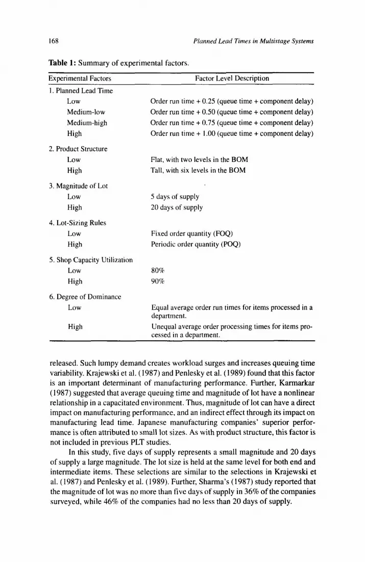
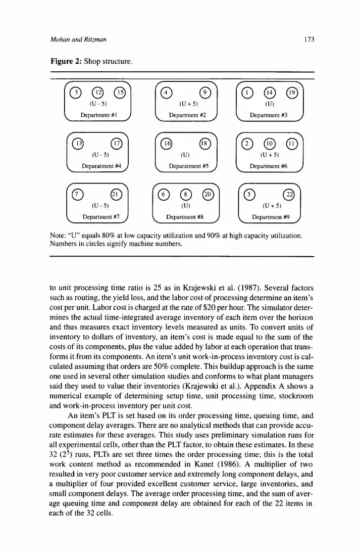
Implementation Issues The manufacturing facility, working in one eight-hour shift each day, has 22 machines organized into nine departments. Five of these departments have two machines each, and the remaining four departments have three machines each. One operator is assigned to each department, and operators are not transferable between departments. Although the shop’s average capacity utilization is set at either 80 or 9096, there are systematic capacity imbalances. Three departments have 5% less than the average capacity utilization, another three departments equal to the average capacity utilization, and the remaining departments 5% more than the average capacity utilization. These capacity imbalances are similar to those in Krajewski et al. (1987) and make the environmental settings more realistic. The utilization setting for the most highly constrained resources was 95%, a level used in several past studies. Figure 2 shows the shop structure with the systematic imbalances that are simulated.

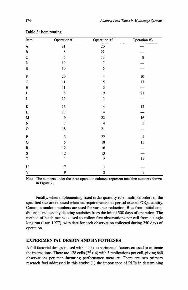
Eleven out of 22 items are routed through two machines, and the remaining items are routed through three machines. An item’s routing length and route are randomly preassigned but remain fixed across the 128 experimental cells. Table 2 shows these individual item routings. No alternative routings are permitted. An item’s routing length is limited to three operations due to computing limitations. That is, a higher number of operations results in larger PLTs and a longer planning horizon especially for the tall product structure. These long planning horizons combined with daily regenerative MRP explosions significantly increase computing requirements.

The setup times and unit processing time at each operation of an item are calculated based on the department utilization, the degree of dominance, the average lot size, and the number of items processed in the department. An item’s setup and unit processing times are deterministic within an experimental cell. The setup time


Figure 2: Shop structure

\

(U + 5 )

Department #1 Department #2

Deparatment #4 Deparatment #5

(“ Department #3 @I Department #6

Department #7 Department #8 Department #9

Note: “U” equals 80% at low capacity utilization and 90% at high capacity utilization. Numbers in circles signify machine numbers.

to unit processing time ratio is 25 as in Krajewski et al. (1987). Several factors such as routing, the yield loss, and the labor cost of processing determine an item’s cost per unit. Labor cost is charged at the rate of $20 per hour. The simulator deter- mines the actual time-integrated average inventory of each item over the horizon and thus measures exact inventory levels measured as units. To convert units of inventory to dollars of inventory, an item’s cost is made equal to the sum of the costs of its components, plus the value added by labor at each operation that trans- forms it from its components. An item’s unit work-in-process inventory cost is calculated assuming that orders are 50% complete. This buildup approach is the same one used in several other simulation studies and conforms to what plant managers said they used to value their inventories (Krajewski et al.). Appendix A shows a numerical example of determining setup time, unit processing time, stockroom and work-in-process inventory per unit cost.

An item’s PLT is set based on its order processing time, queuing time, and component delay averages. There are no analytical methods that can provide accurate estimates for these averages. This study uses preliminary simulation runs for all experimental cells, other than the PLT factor, to obtain these estimates. In these 32 (2s) runs, PLTs are set three times the order processing time; this is the total work content method as recommended in Kanet (1986). A multiplier of two resulted in very poor customer service and extremely long component delays, and a multiplier of four provided excellent customer service, large inventories, and small component delays. The average order processing time, and the sum of average queuing time and component delay are obtained for each of the 22 items in each of the 32 cells.


Table 2: Item routing.

Item Operation #1 Operation #2 Operation #3

A B C D E

F G H I J

K L M N 0

P Q R S T

U v

21 6 6

19 10

20 11 11 8

15

13 17 9 7

18

20 22 13 7 5

4 10 15 17

19 21

- 3

- 1

14 14 22 4

21

12 -

16 5 -

3 22 4 5 18 15

- 12 16 12 13 -

1 2 14

17 9

1 2 7

Note: The numbers under the three operation columns represent machine numbers shown in Figure 2.

Finally, when implementing fixed order quantity rule, multiple orders of the specified size are released when net requirements in a period exceed FOQ quantity. Common random numbers are used for variance reduction. Bias from initial conditions is reduced by deleting statistics from the initial 500 days of operation. The method of batch means is used to collect five observations per cell from a single long run (Law, 1977), with data for each observation collected during 250 days of operation.

EXPERIMENTAL DESIGN AND HYPOTHESES A full factorial design is used with all six experimental factors crossed to estimate the interactions. There are 128 cells (25 x 4) with 5 replications per cell, giving 640 observations per manufacturing performance measure. There are two primary research foci addressed in this study: (1) the importance of PLTs in determining


manufacturing performance, and (2) the effect of operating conditions, represented by the remaining factors, on the relative impact of different PLT levels.

Hypotheses We expect that larger planned lead times would improve customer service because they act as a buffer. At the same time, such larger PLTs may also allow components to remain in the stockroom for a longer period, thereby increasing the inventory level. We expect the cost-benefit relationship to be nonlinear, reflecting diminishing returns to customer service as PLTs are increased more and more. We also expect the impact of PLTs to depend on the operating environment. That is, manufacturing environment with large magnitude of lot, tall product structure, high capacity utilization, and degree of dominance may require a more careful setting of PLTs. Finally, we expect that the two lot-sizing rules will provide a contrast: the POQ rule reducing inventory because of its greater sensitivity to demand, and the FOQ rule will provide a better customer service due to remnants substituting for buffer.

Preliminary Statistical Tests In this study, we use ANOVA to test the statistical hypotheses. Tests for the normal- ity, homogeneity of variance, and independence assumptions of ANOVA are conducted using the SAS software. While all the assumptions are tenable, tests for the error term’s normal distribution parameters suggested that although the mean is zero, the variance increased with the model values. To compensate, the performance measures were transformed using the square root function (Kirk, 1982), and the tests for the assumptions were repeated for the transformed variable. The con- stant variance hypothesis is not rejected with the transformed variable at 5% significance level.

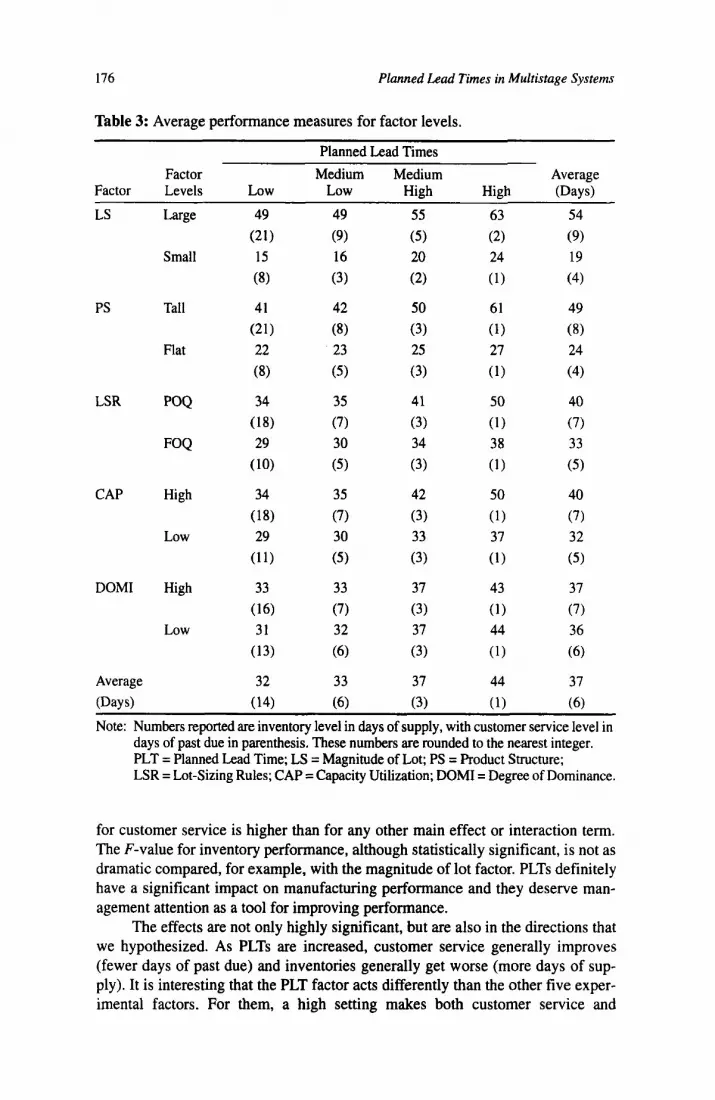
RESULTS FOR PLTs Here we discuss the findings on how planned lead-time changes affect manufacturing performance. ANOVA results for the customer service and inventory measures are provided in Appendix B. Each interaction effect is ranked by its cor- responding level of significance, breaking ties by F-values. Only effects with a probability (P) value not exceeding .01 are reported. The model R2 is .896 when customer service is the dependent variable, and .994 when inventory is the dependent variable. Both ANOVA models are significant at the 1% level. The sum of squares and the mean squares suggest customer service is primarily determined by PLT and magnitude of lot, while inventories depend on the magnitude of lot and product structure. Table 3 shows the direction of the main effects, and interactions between PLTs and the other experimental factors. The means of the performance measures for each factor level are shown in the last row and last column.

Basic Relationships The ANOVA tables in Appendix B show that the main effects of planned lead times on manufacturing performance are highly significant. The F-value of PLTs


Table 3: Average performance measures for factor levels.

Planned Lead Times Factor Medium Medium Average

Factor Levels Low Low High High (Days) LS

PS

LSR

CAP

DOMI

Average

Large

Small

Tall

Flat

POQ

FOQ

High

Low

High

Low

(Days) (14) (6) (3) (1) (6) Note: Numbers reported are inventory level in days of supply, with customer service level in

days of past due in parenthesis. These numbers are rounded to the nearest integer. PLT = Planned Lead Time; LS = Magnitude of Lot; PS = Product Structure; LSR = Lot-Sizing Rules; CAP =Capacity Utilization; DOMI = Degree of Dominance.

for customer service is higher than for any other main effect or interaction term. The F-value for inventory performance, although statistically significant, is not as dramatic compared, for example, with the magnitude of lot factor. PLTs definitely have a significant impact on manufacturing performance and they deserve management attention as a tool for improving performance.

The effects are not only highly significant, but are also in the directions that we hypothesized. As PLTs are increased, customer service generally improves (fewer days of past due) and inventories generally get worse (more days of supply). It is interesting that the PLT factor acts differently than the other five experimental factors. For them, a high setting makes both customer service and

Mohan and Ritzmun 177

inventory worse. Large lot sizes, more stages of manufacture, higher capacity utilization, more order processing time disparities, and POQ (rather than FOQ) all result in worse performance on both dimensions. The PLT factor, on the other hand, represents a managerial trade-off between inventory carrying cost and customer service. To gain more on one dimension, something is given up on the other dimension.

Nonlinearity Further insight comes from Table 3, which shows that customer service improves by 57% (from 14 days of past due to 6 days), 79%, and 92% for the medium-low, medium-high, and high PLT levels, respectively, compared to low PLT levels. The inventory increases that accompany these PLT increases are only 3% (from 32 to 33 days of supply), 1896, and 38%. The reward from the initial PLT increases is an eight days of past due decrease, with the penalty being only a small inventory increase of one day’s supply. As PLTs are increased to the medium-high and high levels, customer service improvements diminish, while inventory increases become more prominent. This nonlinear trade-off relationship has important managerial significance. Decreasing PLTs to reduce inventory is not justified when customer service is poor. Reducing lot sizes and number of levels in product structures are better levers to inventory reduction than small PLTs (see Table 3). However, large PLTs are a poor choice because the benefits of improved customer service may not be justifiable with high inventory levels. That is, when PLTs are increased from medium-low to medium-high levels, customer service improves by three days (from six down to three) but inventories increase by four days of supply. This combination represents a marginal productivity of 0.75 for one day’s inventory (3/4). The next level of PLT increase has a smaller marginal productivity of 0.286 (2/7)-two days improvement in customer service for seven days of inventory. Managers should explore whether safety stock can be more productive than PLTs in improving customer service, especially for PLT ranges beyond medium- high levels.

Co-Component Inventory Disparity The customer service improvements with larger PLTs come from at least two sources. The first source is the end item’s more timely availability. The end item’s larger PLT absorbs more of its manufacturing lead-time variability, just as safety stock absorbs demand quantity variability and increases the probability of the end item’s timely availability.

A second source of customer service improvement is less obvious. Increases in PLTs can help balance inventory placement within the product structure. We illustrate this balancing phenomenon with the tall product structure in Figure 1, in which end item A has items C (component) and D (subassembly) as its two imme- diate co-components. Note that item C’s production does not depend on the availability of other produced items-just one or more purchased items (not shown) that we assume to be available as needed. Item D’s production, by way of contrast, depends on the carefully coordinated production of items E through L. This coordination is not well achieved when PLTs are too short; there is an unintended surplus


in C’s inventory and unintended deficit in item D’s inventory. That is, a small PLT creates an inventory disparity between co-components C and D.

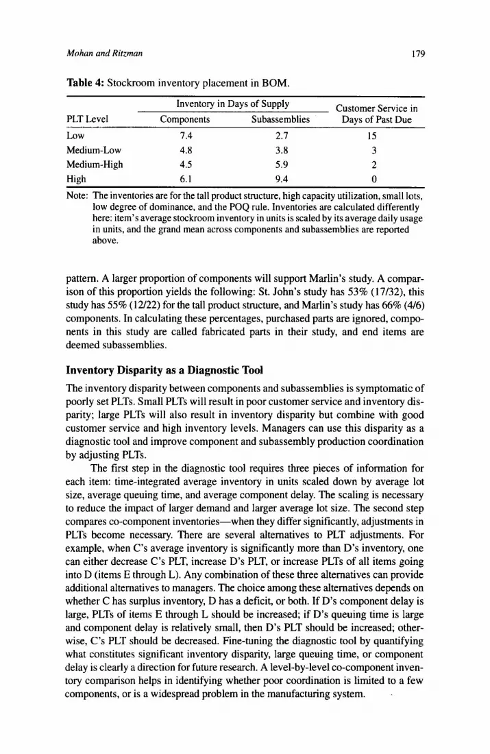
Table 4 documents this inventory disparity between components and subassemblies for the four representative cells that have a tall product structure, high capacity utilization, small lots, low degree of dominance, and the POQ rule. These inventories, also in days of supply, are obtained by dividing the average inventory in units by average demand per day in units. This inventory measure ignores the cost element. At the low PLT level, average inventory is 7.4 days of supply per component, and 2.7 days of supply per subassembly. Excess component inventories, 4.7 days of supply (7.4 - 2.7), do not improve customer service due to insuf- ficient subassembly inventories. This excess component inventory is caused by components being produced (pushed) even when sufficient quantities of subassemblies are unavailable. When subassemblies are eventually produced, it has already delayed its parent’s assembly. The delay in starting the parent’s assembly will eventually hurt customer service. This inventory disparity occurs for all pairs of co-components with C’s inventory more than D’s inventory, F’s inventory more than E’s, G’s inventory more than H’s, and so forth. It also occurs for the components going into end item B. The net result is higher inventory than necessary and poor customer service (1 5 days of past due).

Table 4 shows that increasing PLTs to the medium-low setting reduces the inventory disparity between co-components. Note that components’ inventory decreased even though their PLTs have been increased. The disparity would be smaller if only subassembly PLTs are increased and component PLTs remained at the low level. A subassembly’s more timely availability enables the consumption and reduction of its co-component inventory. For example, D’s more timely availability is due to two factors. First, D’s component delay decreases because all items from E through L that go into D have bigger PLTs and better availability. At the same time, D’s PLT is also increased. The combined effect of a smaller manufacturing lead time and a larger PLT is a significant increase in D’s timely availability and inventory. This timely availability improves A’s production and increases C’s consumption. A‘s higher inventory improves customer service (down to three days of past due demand). The medium-high and high PLT settings con- tinue to increase the subassembly inventory and improve customer service. Com- ponent inventory follows a decrease-increase pattern; at large PLTs, both component and subassembly inventories are large and unproductive.

The improvements in customer service with higher PLTs are consistent with the prior literature (Marlin, 1986; Melnyk & Piper, 1985; Penlesky et al., 1989). The increase in inventory with higher PLTs confirms the findings of St. John (1985), but seems to contradict Kanet (1986) and Marlin. We offer two explanations. First, the types of inventory measure used in these studies are different. Marlin and Kanet measured inventory in number of units and number of hours, not recognizing as we do that subassembly inventory is more costly. Table 5 compares the two types of inventory measure for the representative cells used earlier: Cost-based measure follows St. John’s increasing pattern, and the unit-based measure follows the decrease- increase pattern. Second, the proportion of items that are components in a bill of material affects inventory behavior with PLT increase. Component inventory follows a decrease-increase pattern, but subassembly inventory follows an increasing


Table 4: Stockroom inventory placement in BOM.

Inventory in Days of Supply Customer Service in PLT Level Components Subassemblies Days of Past Due Low 7.4 2.7 15 Medium-Low 4.8 3.8 3 Medium-High 4.5 5.9 2 High 6.1 9.4 0 Note: The inventories are for the tall product structure, high capacity utilization, small lots,

low degree of dominance, and the POQ rule. Inventories are calculated differently here: item’s average stockroom inventory in units is scaled by its average daily usage in units, and the grand mean across components and subassemblies are reported above.

pattern. A larger proportion of components will support Marlin’s study. A comparison of this proportion yields the following: St. John’s study has 53% (17/32), this study has 55% (12/22) for the tall product structure, and Marlin’s study has 66% (4/6) components. In calculating these percentages, purchased parts are ignored, components in this study are called fabricated parts in their study, and end items are deemed subassemblies.

Inventory Disparity as a Diagnostic Tool The inventory disparity between components and subassemblies is symptomatic of poorly set PLTs. Small PLTs will result in poor customer service and inventory disparity; large PLTs will also result in inventory disparity but combine with good customer service and high inventory levels. Managers can use this disparity as a diagnostic tool and improve component and subassembly production coordination by adjusting PLTs.

The first step in the diagnostic tool requires three pieces of information for each item: time-integrated average inventory in units scaled down by average lot size, average queuing time, and average component delay. The scaling is necessary to reduce the impact of larger demand and larger average lot size. The second step compares co-component inventories-when they differ significantly, adjustments in PLTs become necessary. There are several alternatives to PLT adjustments. For example, when C’s average inventory is significantly more than D’s inventory, one can either decrease C’s PLT, increase D’s PLT, or increase PLTs of all items going into D (items E through L). Any combination of these three alternatives can provide additional alternatives to managers. The choice among these alternatives depends on whether C has surplus inventory, D has a deficit, or both. If D’s component delay is large, PLTs of items E through L should be increased; if D’s queuing time is large and component delay is relatively small, then D’s PLT should be increased; otherwise, C’s PLT should be decreased. Fine-tuning the diagnostic tool by quantifying what constitutes significant inventory disparity, large queuing time, or component delay is clearly a direction for future research. A level-by-level co-component inventory comparison helps in identifying whether poor coordination is limited to a few components, or is a widespread problem in the manufacturing system.

180 Planned h a d Times in Multistage Systems

Table 5: Comparison of the two inventory measures.

PLT Level in Days of Supply in Units Cost-Based Measure Unit-Based Measure

Low 22 5947 Medium-Low 26 496 I Medium-High 37 5610 High 53 6535

Note: The inventories are for the tall product structure, high capacity utilization, small lots, low degree of dominance, and the POQ rule.

Kanet (1986) also suggested a diagnostic tool that assumes all stockroom inventories can be classified as either early inventory that is completed early and is waiting for the parent’s assembly date, or delayed inventory that is waiting because other co-components are unavailable. A second assumption is that tardy orders do not wait in the stockroom. Kanet measured inventory in such aggregate terms as hours of output. When early inventory in the system exceeds delayed inventory, PLTs of all items are decreased; when delayed inventory exceeds early inventory, PLTs of all items are increased.

Kanet’s (1986) method poses difficulties in implementation and makes cru- cial assumptions: first, many tardy orders wait in the stockroom; only the last item to arrive that is tardy does not wait in the stockroom. The assumption that tardy orders do not wait in the stockroom become critical when a parent requires several components. In those cases, many co-components may be tardy, but only one of them will avoid the stockroom. Second, delayed and early inventories are not mutually exclusive. For example, when C’s orders are completed early, they wait in the stockroom until the parent’s assembly date and are classified as early inventory. if D is not available by that date, C’s inventory becomes delayed inventory. Third, with part commonality, some units in an order may be delayed inventory and the remaining units may be early inventory because orders can satisfy more than one period’s net requirement. Fourth, aggregate inventory measures such as hours of inventory are useful in identifying overall problems in a PLT setting, but are not effective in identifying localized problems. Kanet’s suggestion to change PLTs for all items may be an ineffective strategy when the problem is limited to a few items.

Interactions The probability values in Appendix B show that interactions between PLT and the remaining five factors are statistically significant. In terms of customer service, the direction of the interactions follow a similar pattern. These five interactions for inventory measure also follow a similar pattern.

Tight PLTs are particularly detrimental when the other factors are likely to cause customer service problems. In other words, relatively larger PLTs are recommended when lot sizes are large, the product structure is tall, the POQ rule is used, and to a lesser extent, the degree of dominance is high. The interactions with product structure and magnitude of lot are particularly strong. Increases in inventories


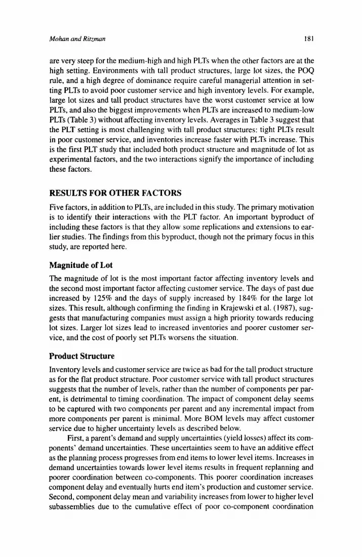
are very steep for the medium-high and high PLTs when the other factors are at the high setting. Environments with tall product structures, large lot sizes, the POQ rule, and a high degree of dominance require careful managerial attention in setting PLTs to avoid poor customer service and high inventory levels. For example, large lot sizes and tall product structures have the worst customer service at low PLTs, and also the biggest improvements when PLTs are increased to medium-low PLTs (Table 3) without affecting inventory levels. Averages in Table 3 suggest that the PLT setting is most challenging with tall product structures: tight PLTs result in poor customer service, and inventories increase faster with PLTs increase. This is the first PLT study that included both product structure and magnitude of lot as experimental factors, and the two interactions signify the importance of including these factors.

RESULTS FOR OTHER FACTORS Five factors, in addition to PLTs, are included in this study. The primary motivation is to identify their interactions with the PLT factor. An important byproduct of including these factors is that they allow some replications and extensions to earlier studies. The findings from this byproduct, though not the primary focus in this study, are reported here.

Magnitude of Lot The magnitude of lot is the most important factor affecting inventory levels and the second most important factor affecting customer service. The days of past due increased by 125% and the days of supply increased by 184% for the large lot sizes. This result, although confirming the finding in Krajewski et al. (1987), suggests that manufacturing companies must assign a high priority towards reducing lot sizes. Larger lot sizes lead to increased inventories and poorer customer service, and the cost of poorly set PLTs worsens the situation.

Product Structure Inventory levels and customer service are twice as bad for the tall product structure as for the flat product structure. Poor customer service with tall product structures suggests that the number of levels, rather than the number of components per parent, is detrimental to timing coordination. The impact of component delay seems to be captured with two components per parent and any incremental impact from more components per parent is minimal. More BOM levels may affect customer service due to higher uncertainty levels as described below.

First, a parent’s demand and supply uncertainties (yield losses) affect its components’ demand uncertainties. These uncertainties seem to have an additive effect as the planning process progresses from end items to lower level items. Increases in demand uncertainties towards lower level items results in frequent replanning and poorer coordination between co-components. This poorer coordination increases component delay and eventually hurts end item’s production and customer service. Second, component delay mean and variability increases from lower to higher level subassemblies due to the cumulative effect of poor co-component coordination

182 Plumed Lead Times in Multistage Systems

from low-level through higher level items. A subassembly’s higher component delay variability increases in coordinating co-component production. An increasing demand uncertainty from high- to low-level items, and increasing timing uncertainty from low- to high-level items make tall product structures inherently more difficult to plan. Finally, the planning horizon for tall product structure is longer than that for flat product structure even if individual items have identical PLTs in the two product structures. Longer planning horizons commit productive resources much before they are required, and such early commitment is detrimental especially when demand, supply, and manufacturing lead-time variabilities are higher.

The poorer customer service for the tall product structures agrees with the conclusions in Fry et al. (1989) and Ritzman and Krajewski (1983), but disagrees with those in Bott and Ritzman (1983). The contradiction may be explained by how product structure changes are introduced in the experiment. Here the manufacturing requirements of each item, A through V in Figure 1, are retained for both tall and flat product structures in all experimental cells. For example, item D is always routed to the same departments and in the same sequence. Only processing and setup times are changed so that other factors such as magnitude of lot do not distort the desired capacity utilization levels. Such close control over item identity is not done in Bott and Ritzman.

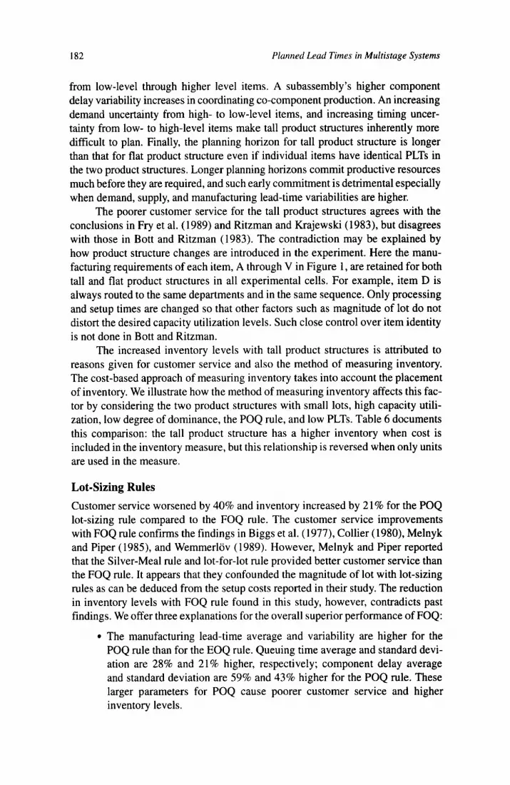
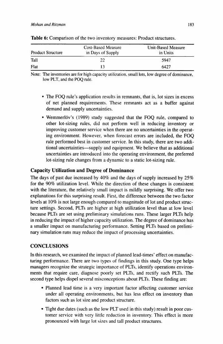
The increased inventory levels with tall product structures is attributed to reasons given for customer service and also the method of measuring inventory. The cost-based approach of measuring inventory takes into account the placement of inventory. We illustrate how the method of measuring inventory affects this factor by considering the two product structures with small lots, high capacity utilization, low degree of dominance, the POQ rule, and low PLTs. Table 6 documents this comparison: the tall product structure has a higher inventory when cost is included in the inventory measure, but this relationship is reversed when only units are used in the measure.

Lot-Sizing Rules Customer service worsened by 40% and inventory increased by 21% for the POQ lot-sizing rule compared to the FOQ rule. The customer service improvements with FOQ rule confirms the findings in Biggs et al. (1977), Collier (1980), Melnyk and Piper (1985), and Wemmerlov (1 989). However, Melnyk and Piper reported that the Silver-Meal rule and lot-for-lot rule provided better customer service than the FOQ rule. It appears that they confounded the magnitude of lot with lot-sizing rules as can be deduced from the setup costs reported in their study. The reduction in inventory levels with FOQ rule found in this study, however, contradicts past findings. We offer three explanations for the overall superior performance of FOQ:

The manufacturing lead-time average and variability are higher for the POQ rule than for the EOQ rule. Queuing time average and standard deviation are 28% and 21% higher, respectively; component delay average and standard deviation are 59% and 43% higher for the POQ rule. These larger parameters for POQ cause poorer customer service and higher inventory levels.


Table 6: Comparison of the two inventory measures: Product structures.

Cost-Based Measure Unit-Based Measure Product Structure in Days of Supply in Units Tall Flat

22 13

5947 6427

~~~~~

Note: The inventories are for high capacity utilization, small lots, low degree of dominance, low PLT, and the POQ rule.

The FOQ rule’s application results in remnants, that is, lot sizes in excess of net planned requirements. These remnants act as a buffer against demand and supply uncertainties.

Wemmerlov’s (1989) study suggested that the FOQ rule, compared to other lot-sizing rules, did not perform well in reducing inventory or improving customer service when there are no uncertainties in the operating environment. However, when forecast errors are included, the FOQ rule performed best in customer service. In this study, there are two additional uncertainties-supply and equipment. We believe that as additional uncertainties are introduced into the operating environment, the preferred lot-sizing rule changes from a dynamic to a static lot-sizing rule.

Capacity Utilization and Degree of Dominance The days of past due increased by 40% and the days of supply increased by 25% for the 90% utilization level. While the direction of these changes is consistent with the literature, the relatively small impact is mildly surprising. We offer two explanations for this surprising result. First, the difference between the two factor levels at 10% is not large enough compared to magnitude of lot and product structure settings. Second, PLTs are higher at high utilization level than at low level because PLTs are set using preliminary simulations runs. These larger PLTs help in reducing the impact of higher capacity utilization. The degree of dominance has a smaller impact on manufacturing performance. Setting PLTs based on preliminary simulation runs may reduce the impact of processing uncertainties.

CONCLUSIONS In this research, we examined the impact of planned lead-times’ effect on manufacturing performance. There are two types of findings in this study. One type helps managers recognize the strategic importance of PLTs, identify operations environments that require care, diagnose poorly set PLTs, and rectify such PLTs. The second type helps dispel several misconceptions about PLTs. These finding are:

Planned lead time is a very important factor affecting customer service under all operating environments, but has less effect on inventory than factors such as lot size and product structure.

Tight due dates (such as the low PLT used in this study) result in poor customer service with very little reduction in inventory. This effect is more pronounced with large lot sizes and tall product structures.

I84 Planned Lead Times in Multistage Systems

Small amounts of PLT increases improve customer service substantially. This improvement is achieved with small inventory increases. Further PLT increases result in diminishing customer service improvements, but the inventory levels grow faster.

PLT changes affect co-component inventories in a product structure. A high inventory disparity with poor customer service is indicative of tight PLTs and with excellent customer service, and high inventory levels may indicate large PLTs. Managers can use inventory disparities as a diagnostic tool to detect problems in PLTs.

PLT setting in tall product structures requires careful consideration, because tight due dates hurt customer service severely and loose due dates increase inventories substantially. That is, timing coordination through a proper PLT setting must carefully consider the parent-component relationship similar to quantity coordination achieved through deriving component gross requirements from parent order schedules.

This study was useful in dispelling several misconceptions about PLTs: (1) PLTs are an important strategic decision that need further investigation and do not justify the lack of past efforts. (2) PLTs should not be as small as possible. PLTs may be set based on manufacturing lead time, but they are not synonymous. Man- agers must distinguish this difference between PLTs and manufacturing lead time. Efforts to reduce manufacturing lead times, as done in time-based competition, are laudatory, but should not be confused with keeping PLTs small. (3) The disparity between planned and actual lead times is important. Tight PLTs provide poor customer service but not the advantages of lower inventory, and large PLTs may provide excellent customer service but at high inventory levels. The nonlinear relationship between the two manufacturing performance measures suggest that setting PLTs should reflect the objectives and the competitive priorities of the organization, and should avoid extreme PLTs. (4) Differences between cost-based and unit-based inventory measures can lead to contradicting conclusions about the behavior of inventory as PLTs are increased.

We suggest that a balanced inventory placement in the BOM is a key to improved customer service. The superior performance of the FOQ rule, especially in terms of inventory, is a surprising result. The notion that static lot-sizing rules are preferable to the dynamic lot-sizing rules when several uncertainties are present needs further investigation. The remaining conclusions, such as the impact of large lot sizes and high capacity utilization, confirm earlier findings.

In reaching these conclusions, we opted for a research approach that makes the environmental settings as realistic as possible. Another approach is to tighten the focus of the study and simplify the assumptions made. For example, there can be a downside to our research approach. Introducing fixed factors such as forecast errors, equipment failures, and imperfect quality eliminates many useful method- ologies and makes a methodology such as simulation more complex. These noise factors can increase the error term in analysis of variance, and important effects caused by the experimental factors may not be found to be statistically significant. Thus, both research styles are needed and add value. [Received: August 24, 1994. Accepted: January 14, 1997.1


REFERENCES Amoako-Gyampah, K., & Meredith, J. R. (1989). The operations management

research agenda: An update. Journal of Operations Management, 8(3), 250- 262.

Anderson, J. C., Schroeder, R. G., Tupy, S. E., & White, E. M. (1982). Material requirements planning systems: The state of the art. Production andlnventory Management, 23(4), 5 1-66.

Bahl, H. C., Ritzman, L. P., & Gupta, J. N. D. (1987). Determining lot sizes and resource requirements: A review. Operations Research, 35(3), 329-345,

Benton, W. C., & Srivastava, R. (1985). Product structure complexity and multi- level lot sizing using alternative costing policies. Decision Sciences, 16(4),

Blackburn, J. D., & Millen, R. A. (1982). Improved heuristics for multi-stage requirements planning systems. Management Science, 28( l ) , 44-56.

Bott, K. N., & Ritzman, L. P. (1983). Irregular workloads with MRP systems: Some causes and consequences. Journal of Operations Management, 3(4),

Collier, D. A. (1980). A comparison of MRP lot sizing methods considering capacity change costs. Journal of Operations Management, I I ( l ) , 23-29.

Collier, D. A. (198 1). The measurement and operational benefits of component part commonality. Decision Sciences, 12( 1 ), 85-96.

Fry, T. D., Oliff, M. D., Minor, E. D., & Leong, G. K. (1989). The effects of product structure and sequencing rule on assembly shop performance. International Journal of Production Research, 27(4), 67 1-686.

Grasso, E. T., & Taylor, B. W., 111. (1984). A simulation-based experimental investigation of supplyhiming uncertainty. International Journal of Production Research, 22(3), 485-497.

Hoyt, J. (1978). Dynamic lead times that fit today’s dynamic planning (Q.U.O.A.T. lead time). Production and Inventory Management, I9( l ) , 63-70.

Kanet, J. J . (1986). Toward a better understanding of lead times in MRP systems. Journal of Operations Management, 6(3), 305-3 15.

Karmarkar, U. S. (1987). Lot sizes, lead times and in-process inventories. Management Science, 33(3), 409-4 18.

Kirk, R. E. (1982). Experimental design: Prucedures for the behavioral sciences. Reading, CA: Brooks/Cole Publishing Company.

Krajewski, L. J., King, B. E., Ritzman, L. P., & Wong, D. S. (1987). Kanban, MRP, and shaping the manufacturing environment. Management Science, 33( 1),

LaForge, R. L., & Sturr, V. L. (1986). MRP practices in a random sample of manufacturing firms. Production and Inventory Management, 27(3), 129- 137.

357-369.

169- 182.

29-57.


Law, A. M. (1977). Confidence intervals in discrete event simulation: A comparison of replication and batch means. Naval Research Logistics Quarterly, 24, 667-678.

Malhotra, M. K., & Ritzman, L. P. (1990). Resource flexibility issues in multistage manufacturing. Decision Sciences, 21,673-690.

Marlin, P. G. (1986). Manufacturing lead time accuracy. Journal of Operations Management, 6(2), 179-202.

McCleland, M. K., & Wagner, H. M. (1988). Location of inventories in an MRP environment. Decision Sciences, 19(3), 535-553.

Melnyk, S. A., & Piper, C. J. (1985). Lead time errors in MRP: The lot-sizing effect. International Journal of Production Research, 23(2), 253-264.

Mohan, R. P., & Ritzman, L. P. (1989). Towards understanding lead times: Four key factors. Proceedings of the Decision Sciences Institute Annual Meeting,

Orlicky, J. ( 1975). Material requirements planning. Reading, NY McGraw Hill Book Company.

Penlesky, R. J., Berry, W. L., & Wemmerlov, U. (1989). Open order due date maintenance in MRP systems. Management Science, 35(5), 57 1-584.

Plossl, G. W., & Welch, W. E. (1979). The role of top management in the control of inventory. Reading, VA: Reston Publishing Company, Inc.

Ragatz, G. L. (1989). A note on workload-dependent due date assignment rules. Journal of Operations Management, 8(4), 377-384.

Rammohan, P. (1991). Planned lead times for material requirements planning systems. Unpublished doctoral dissertation, The Ohio State University.

Ritzman, L. P., & King, B. E (1993). The relative significance of forecast errors in multistage manufacturing. Journal of Operations Management, I I , 5 1-65.

Ritzman, L. P., & Krajewski, L. J. (1983). Comparison of material requirements planning and reorder point systems. In H. Bekroglu (Ed.), Simulation and inventory control. The Ohio State University, Society for Computer Simulation.

Sharma, D. (1987). Manufacturing strategy: An empirical analysis. Unpublished doctoral dissertation, The Ohio State University.

St. John, R. (1985). The cost of inflated planned leadtimes in MRP systems. Journal of Operations Management, 5(2), 11 9- 128.

Weeks, J. K. (1978). Optimizing planned lead times and delivery date. Proceedings of the 21st American Production and Inventory Control Society Annual Meeting, 177-188.

Wemmerlov, U. (1989). The behavior of lot-sizing procedures in the presence of forecast errors. Journal of Operations Management, 8( 1 ), 37-54.

Whybark, D. C., & William, J. G. (1976). Material requirements planning under uncertainty. Decision Sciences, 17(4), 595-606.

Yano, C. A. (1987a). Planned leadtimes for serial production system. IIE Transactions, 19(3), 300-307.

948-950.


Yano, C. A. (1987b). Stochastic leadtimes in two-level assembly systems. ZZE

Yano, C. A. (1987~). Setting planned leadtimes in serial production systems with Transactions, 19(4), 37 1-378.

tardiness costs. Management Science, 33( l), 95-106.

APPENDIX A

Example Calculation for Unit Processing Time, Setup Time, and Unit Costs Example calculations for item A, with tall product structure, low average shop capacity utilization, and low magnitude of lot.

a. Unit processing and setup time for low degree of dominance.

Item A is processed first at Machine #21 (Table 2), which is in Department #7 (Fig- ure 2). This department’s capacity utilization is 75%, which translates to 6 hours availability per day for order processing and machine repairing based on an 8-hour shift. Machine repairs require, on the average, 14 hours for every 480 hours of order processing. That is, the time available for processing items is 5.8300 hours (480 x 6/494).

Department #7 has Machines #7 and #21. These two machines process items D, N, and V in Machine #7, and items A, I, and 0 in #21. The following symbols are used:

OPi

Si

Ui Lsi

= Item i’s average order processing time in Department #7.

= Item i’s setup time in Department #7.

= Item i’s unit processing time in Department #7.

= Item i’s average lot size.

Since, setup-to-unit processing time ratio is 25, Si = 25Ui. At low magnitude of lot, lot sizes cover 5 days of demand. For end item A, the lot size is 100 good units (20 x 5). At 5 % average yield loss, the order size when released is 105 units, that is, loo/( 1 - 0.95).

OPA = SA i- LSA X UA

= 25uA LsA x r /A

= 130U~.

That is, Department #7 must “process” an average 130 units over 5 days, or 26 units each day. When degree of dominance is low, order processing times for all the six items are equal.

OPA = OPD = oP1= OPN = OPO = OPV.

That is, item A uses one-sixth of the productive time each day. So, 26 units require 0.9717 hours (5.8300/6), and each unit requires 135 seconds (0.9717 x 3600/26). The setup time is 3,364 seconds (0.97 17 x 3600 x 25/26).


A similar calculation for A's second operation will result in a unit processing time of 144 seconds, and 3,588 seconds of setup time.

b. Stockroom and work-in-process unit costs The following symbols are used:

Ci = Item i's stockroom per unit cost.

WZPi = Item i's work-in-process per unit cost.

Value added, at the rate of $20 per hour, to the 105 units of item A equals value added at the first operation plus value added at the second operation and equals:

{ (3364 + 105 x 133) + (3588 + 105 x 144)) x 20 3600

$200.21.

The total cost for the 105 units of item A equals 105 units each of components C and D, and the value added at the two operations: 105(Cc + CD) + $200.21. Among these 105 units, only 100 good units will be available on average. The cost of one unit of end item A is:

105(C, + C,) + 200.21 100

CA =

Work in process is assumed to be 50% complete, and the cost per unit is based on 105 units because goods are rejected after the final operation:

105(C, + C,) + 0.50 x 200.21 105

WIP, =

c. Unit processing and setup time for high degree of dominance When degree of dominance is high, order processing times are unequal. That is,

OPA = OPD = OP1= 4 0 P ~ = 4oPo = 40Pv.

So, 26 units require 1.5547 hours (4 x 5.8300/15), or unit processing time is 215 seconds, and setup time is 5,382 seconds.


APPENDIX B

Analyses of Variance

a. Customer Service Performance Measure (Days of Past Due) ~

Source Degrees of Freedom Sum of Squares Mean Square

Model 127 979.77 7.71 Error 512 113.30 0.22 Corrected Total 639 1093.07 F-Value = 34.86 R2 = 396 P > F = .oooO

Degrees of ANOVA Mean Source Freedom ss Square F-Value P > F T M P L C D T*P M*P T*M M*D T*L T*C M*L L*D P*C

3 1

1 1 1 1 3 1

3 1 3 3 1

1

1

500.77 158.06 24.23 13.27 9.59 4.46

70.5 1 22.99 36.11 11.55 24.19 22.62 4.27 2.7 1

2.29

166.92 158.06 24.23 13.27 9.59 4.46

23.50 22.90 12.04 11.55 8.06 7.54 4.27 2.7 1

2.29

754.34 714.28 109.51 59.97 43.34 20.13

106.52 103.89 54.40 52.18 36.44 34.07 19.30 12.26 10.33

.moo

.moo

.0001

.ooo1

.000 1

.ooo 1

.ooo 1

.ooo 1

.0001

.ooo 1

.0001

.o001

.ooo I

.0005

.oo14

Notes: Only main effects and first-order interactions significant at a level greater than 0.01 are included. P = Product Structure; M = Magnitude of Lot; L = Lot-Sizing Rules; T = Planned Lead Time; C = Capacity Utilization; D = Degree of Dominance; * = Interaction. The complete ANOVA results are available upon request.


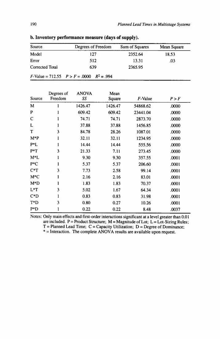
b. Inventory performance measure (days of supply).

Source Degrees of Freedom Sum of Squares Mean Square

Model Error Corrected Total

127 512 639

F-Value = 712.55 P > F = .oooO R2 = .994

2352.64 18.53 13.31 .03

2365.95

Degrees of ANOVA Mean Source Freedom ss Sauare F-Value P > F M P C L T M*P P*L P*T M*L P*C C*T M*C M*D L*T C*D T*D

1 1 1 1 3 1 1 3 1 1 3 1 1 3 1 3

1426.47 609.42 74.71 37.88 84.78 32.11 14.44 21.33 9.30 5.37 7.73 2.16 1.83 5.02 0.83 0.80

1426.47 609.42 74.7 1 37.88 28.26 32.11 14.44 7.11 9.30 5.37 2.58 2.16 1.83 1.67 0.83 0.27

54868.62 23441.04

2873.70 1456.85 1087.01 1234.95 555.56 273.45 357.55 206.60 99.14 83.01 70.37 64.34 31.98 10.26

.moo

.OoOo

.moo

.moo

.moo

.moo

.OoOo

.OoOo

.mo1

.om1

.ooo 1

.ooo 1

.ooo 1

.ooo1

.ooOl

.ooo1 P*D 1 0.22 0.22 8.48 .oo37

Notes: Only main effects and first-order interactions significant at a level greater than 0.01 are included. P = Product Structure; M = Magnitude of Lot; L = Lot-Sizing Rules; T = Planned Lead Time; C = Capacity Utilization; D = Degree of Dominance; * = Interaction. The complete ANOVA results are available upon request.

Mohan and R i t m n 191

Ram P. Mohan is a senior manufacturing consultant at Adapta Solutions, Inc., Hawthorne, New York. He was previously an assistant professor at Baruch College, CUNY. He earned his Ph.D. in operations management from The Ohio State University. He has an MBA and a BS in mechanical engineering. Dr. Mohan is a member of the Decision Sciences Institute. His research interests include production planning and control, and manufacturing lead time.

Larry P. Ritzman is the Thomas J. Galligan, Jr., Professor of Operations and Strategic Management at Boston College. He received his doctorate from Michigan State University. Dr. Ritzman’s research and teaching interests are in production and inventory systems, operations strategy, layout, and forecasting. He has published in a number of journals, including Decision Sciences, Journal of Operations Management, Management Science, Operations Research, Harvard Business Review, Integaces, and International Journal of Production Research. He is a past president of the Decision Sciences Institute and is also a member of INFORMS and POMS.

planned lead times in multistage systems

Documents