energies

Article

Numerical Investigation on Bubble Distribution ofa Multistage Centrifugal Pump Based on a PopulationBalance Model

Sina Yan, Shuaihui Sun *, Xingqi Luo *, Senlin Chen, Chenhao Li and Jianjun Feng

State Key Laboratory of Eco-hydraulics in Northwest Arid Region, Xi’an University of Technology, Xi’an 710048,China; 18702970872@163.com (S.Y.); chensl@xaut.edu.cn (S.C.); drleech_xaut@126.com (C.L.);18802936315@163.com (J.F.)* Correspondence: shs@xaut.edu.cn (S.S); luoxq@xaut.edu.cn (X.L.)

Received: 17 January 2020; Accepted: 10 February 2020; Published: 18 February 2020�����������������

Abstract: This work aimed to study the bubble distribution in a multiphase pump. A Euler-Eulerinhomogeneous two-phase flow model coupled with a discrete particle population balance model(PBM) was used to simulate the whole flow channel of a three-stage gas-liquid two-phase centrifugalpump. Comparison of the computational fluid dynamic (CFD) simulation results with experimentaldata shows that the model can accurately predict the performance of the pump under variousoperating conditions. In addition, the liquid phase velocity distribution, gas-phase distribution,and pressure distribution of the second stage impeller at a 0.5 span of blade height under threetypical working conditions were compared. Results show that the region with high local gas volumefraction (LGVF) mainly appears on the suction surface (SS) of the blade. With the increase in inlet gasvolume fraction (IGVF), vortices and low velocity recirculation regions are generated at the impelleroutlet and SS of the blade, the area with high LGVF increases, and gas–liquid separation occurs atthe SS of the blade. The liquid phase flows out of the impeller at high velocity along the pressuresurface of the blade, and the limited pressurization of fluid mainly happens at the impeller outlet.The average bubble size at the impeller outlet is the smallest while that at the impeller inlet is thelargest. Under low IGVF conditions, bubbles tend to break into smaller ones, and the broken bubblesmainly concentrate at the blade pressure surface (PS) and the impeller outlet. Bubbles tend to coalesceinto larger ones under high IGVF conditions. With the increase in IGVF, the bubble aggregation zonediffuses from the blade SS to the PS.

Keywords: centrifugal pump; bubble distribution; numerical simulation; population balance model

1. Introduction

Multistage centrifugal pumps have been widely used in the field of oil gas mixed transportationdue to their advantages of high head, high efficiency, and simple structure [1,2]. The multi-stagecentrifugal pump needs to operate under different inlet gas volume fraction (IGVF) conditions, asthe volume fraction of oil and gas always changes during crude oil production and transportation.At low IGVF conditions, the pump has a higher head and efficiency, but under high IGVF conditions,its pressurization capacity drops sharply or it even stops working, which seriously endangers thecontinuity and safety of industrial production [3]. Therefore, it is of great significance to carry outan investigation on gas–liquid two-phase flow in a multistage centrifugal pump and improve itsperformance at IGVF conditions.

Many scholars have studied the flow characteristics in gas-liquid two-phase flow pumps.Caridad [4] pointed out that the accumulation of gas-phase on the blade surface caused the performance

Energies 2020, 13, 908; doi:10.3390/en13040908 www.mdpi.com/journal/energies

Energies 2020, 13, 908 2 of 15

of the centrifugal pump to decrease, and the air pocket increases with the increase of the IGVF whenthe flow rate is identical. Poullikkas [5] studied the effect of a gas–liquid two-phase flow on theperformance of a centrifugal nuclear main pump. The author pointed out that the accumulationof gas-phase in the impeller flow channel changes the liquid flow direction, narrows the effectiveflow area, and causes the pump performance to decrease. Verde [6] divided the flow patterns ofthe centrifugal pump impellers into bubbly flow, agglomerated bubble flow, gas pocket flow, andsegregated flow according to the morphology of the gas-liquid two-phase medium distribution. It waspointed out that the change of flow pattern of the impeller caused the pump performance to decline,especially the gas pocket in the impeller, which caused unstable pump operation. Si [7] pointed outthat the accumulation of bubbles in the impeller of the centrifugal pump affects the energy exchangeand transfer in the impeller, and the vortices in the impeller also intensify the accumulation of bubbles.Results showed that bubbles first gather on the suction surface of the blade, and the accumulationarea diffuses to the entire impeller flow channel as the IGVF increases. Zhang [8] investigated thebubble size distribution in a three-stage helico-axial flow pump under different IGVFs. Results showedthat the larger IGVF, the larger the average diameter and the peak diameter of the bubble in the flowfield. It can be seen that the bubble accumulation causes flow pattern changes and performancedegradation in the pump, and bubble coalescence and break up are closely related to the IGVF andthe size of bubbles. However, the relationship between bubble diameter and bubble coalescence, aswell as bubbles broken in multi-stage centrifugal pumps, is still unclear, which hinders the pump’sperformance improvement under high IGVF conditions.

Two methods are commonly used for studying the internal flow of a gas–liquid two-phase flowpump: experimental [9–11] and numerical simulation methods [12]. The second method has beenwidely used because of its low cost, high reliability, and more intuitive reflection of the internal flowfield. Many scholars [13,14] obtained computational fluid dynamic (CFD) simulation results thatagreed well with the experimental data under IGVF conditions on gas–liquid two-phase flow pumps.However, the forces of gas-liquid two-phase flow pumps in rotating machines are very complexunder high gas volume fraction conditions, such as centrifugal force, shear force, drag force, andbuoyancy, which cause gas–liquid separation and hinder the accurate prediction of pump performanceby numerical simulation. Caridad [15] conducted a numerical simulation of a centrifugal pump basedon a 3D two-phase flow model coupled with a single bubble size model. Their simulations agreedwith the experimental data under low IGVF conditions, and the numerical simulation results werelarger than the experimental values under high IGVF conditions. Zhu [16] performed numericalcalculations using the bubble size model of Barrios [17] and Gamboa [18]. Results showed that theerror of numerical simulation results using the bubble size model was larger than the experimentalvalue. Therefore, the semi-empirical formula of the bubble size model has its limitations. Frank [19]and Lilunnahar [20] et al. investigated the gas-phase distribution, liquid flow velocity, and bubblesize distribution in different sections of a vertical pipe by using a population balance model (PBM)model that considers bubble forces, bubble coalescence, and bubble break up. The results showed thatthis model is suitable for the numerical simulation of a gas-liquid two-phase flow under any IGVFoperating conditions. Multiple groups of bubble sizes are set in the PBM model, which considers thebreakup and coalescence of bubbles. This model can more closely reflect the distribution of bubble sizegroups in the two-phase flow field. Therefore, the results obtained by using this model to simulate thegas–liquid two-phase flow field are more accurate. There are few cases [21] in which the PBM modelis applied to a gas-liquid two-phase numerical simulation of rotating machinery, and the predictionaccuracy for the gas-liquid two-phase rotating machinery performance is not clear.

In the present work, the population balance model was applied to a gas-liquid two-phase flowthree-stage centrifugal pump with rotating components by using ANSYS CFX 18.0. The numericalsimulation results were compared with the experimental results to verify the accuracy of the numericalsimulation. The pressure increase characteristics and internal flow field characteristics of the pumpunder different IGVFs were analyzed, and the gas-liquid two-phase distribution area, bubble coalescence

Energies 2020, 13, 908 3 of 15

area, and break up area were obtained. This research provides an idea for more accurately predictingthe performance of gas–liquid two-phase flow pumps, and a reference for design and optimization ofgas-liquid two-phase flow centrifugal pumps.

2. Experimental Test Rig and Pump Model

2.1. Experimental Test Rig

The gas–liquid two-phase experimental system of a three-stage centrifugal pump is shown inFigure 1. It is a branch system of a large-scale deep-sea gathering and transmission experimentalsystem of State Key Laboratory of Multiphase Flow in Power Engineering, Xi’an Jiaotong University.

Energies 2020, 13, x FOR PEER REVIEW 3 of 15

2. Experimental Test Rig and Pump Model

2.1. Experimental Test Rig

The gas–liquid two-phase experimental system of a three-stage centrifugal pump is shown in Figure 1. It is a branch system of a large-scale deep-sea gathering and transmission experimental system of State Key Laboratory of Multiphase Flow in Power Engineering, Xi’an Jiaotong University.

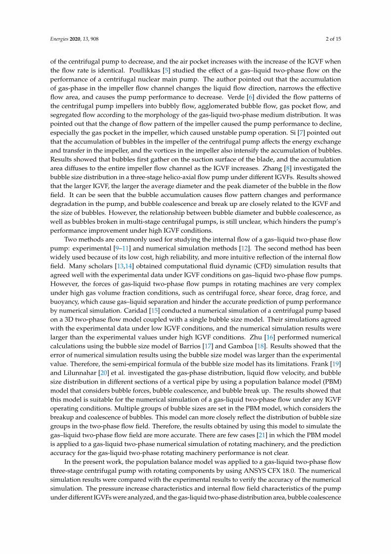
Figure 1. Experimental flow loop of a gas-liquid two-phase three-stage pump: ① air compressor, ② gas buffer tank, ③ gas mass flowmeter, ④ plunger pump, ⑤ liquid mass flowmeter, ⑥ gas-liquid mixing section, ⑦ gas–liquid mixer, ⑧ experimental pump, ⑨ torque tachometer, ⑩ electric motor, ⑪ pneumatic control valve, ⑫ gas-liquid separator, ⑬ micropore muffler, ⑭ water tank, ⑮ backflow valve.

This system is composed of a gas-phase line, a liquid-phase line, and a gas-liquid mixture line. In the gas-phase line, air passes through the compressor and enters the gas buffer tank to stabilize the pressure. After passing through the gas mass flowmeter, it finally enters the gas–liquid mixing section. In the liquid-phase line, the water from the water tank is pressurized by the plunger pump, passes through the liquid mass flowmeter, and finally enters the gas-liquid mixing section to mix with the air. In the gas–liquid mixture line, the gas-liquid phase mixed by the mixer enters the experimental pump and finally returns to the gas-liquid separator. The test rig of the experimental section is shown in Figure 2. The RHM30 and RHM06 high-precision mass flow meters were used to measure the flow rate of air and water. The gas and liquid phase measurement accuracy is 0.5% and 0.15%, respectively. The inlet pressure, outlet pressure, and pressure differentials between pump inlet and outlet of the experimental pump were measured by Rosemount 3051 series pressure and differential pressure sensors with a measurement accuracy of 0.075%. The HY-5005 torque tachometer was used to measure the torque and rotational speed of the pump, and its accuracy is 0.1%. The experimental test maintains the pump rotational speed, inlet pressure, and liquid phase mass flow rate under different IGVFs at an identical value to investigate the effect on the pump performance by adjusting the air volume fraction λg at the pump inlet. The experimental parameters are as follows: pump rotational speed is 3500 rpm, high pressure inlet, water mass flow rate is 7.2 kg/s, and the IGVF λg of the pump ranges from 0% to 25.7%. The expression of the IGVF λg is shown in Equation (1).

1gg

g ll

QQ Q

λ λ= = −+

(1)

where, Qg and Ql represent the gas and liquid volume flow rate, respectively, in m3/h. λl represents the liquid volume fraction, in %.

Figure 1. Experimental flow loop of a gas-liquid two-phase three-stage pump: 1O air compressor, 2O gasbuffer tank, 3O gas mass flowmeter, 4O plunger pump, 5O liquid mass flowmeter, 6O gas-liquid mixingsection, 7O gas–liquid mixer, 8O experimental pump, 9O torque tachometer, 10O electric motor, 11O pneumaticcontrol valve, 12O gas-liquid separator, 13Omicropore muffler, 14Owater tank, 15O backflow valve.

This system is composed of a gas-phase line, a liquid-phase line, and a gas-liquid mixture line.In the gas-phase line, air passes through the compressor and enters the gas buffer tank to stabilize thepressure. After passing through the gas mass flowmeter, it finally enters the gas–liquid mixing section.In the liquid-phase line, the water from the water tank is pressurized by the plunger pump, passesthrough the liquid mass flowmeter, and finally enters the gas-liquid mixing section to mix with the air.In the gas–liquid mixture line, the gas-liquid phase mixed by the mixer enters the experimental pumpand finally returns to the gas-liquid separator. The test rig of the experimental section is shown inFigure 2. The RHM30 and RHM06 high-precision mass flow meters were used to measure the flowrate of air and water. The gas and liquid phase measurement accuracy is 0.5% and 0.15%, respectively.The inlet pressure, outlet pressure, and pressure differentials between pump inlet and outlet of theexperimental pump were measured by Rosemount 3051 series pressure and differential pressuresensors with a measurement accuracy of 0.075%. The HY-5005 torque tachometer was used to measurethe torque and rotational speed of the pump, and its accuracy is 0.1%. The experimental test maintainsthe pump rotational speed, inlet pressure, and liquid phase mass flow rate under different IGVFs at anidentical value to investigate the effect on the pump performance by adjusting the air volume fractionλg at the pump inlet. The experimental parameters are as follows: pump rotational speed is 3500 rpm,high pressure inlet, water mass flow rate is 7.2 kg/s, and the IGVF λg of the pump ranges from 0% to25.7%. The expression of the IGVF λg is shown in Equation (1).

λg =Qg

Qg + Ql= 1− λl (1)

where, Qg and Ql represent the gas and liquid volume flow rate, respectively, in m3/h. λl representsthe liquid volume fraction, in %.

Energies 2020, 13, 908 4 of 15Energies 2020, 13, x FOR PEER REVIEW 4 of 15

Figure 2. Test rig of the experimental setup.

2.2. Computing Domain and Mesh Generation

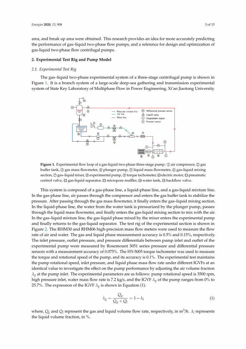
The gas–liquid two-phase flow pump used in the experiment is a three-stage centrifugal pump with a specific speed of 26.6. The pump design volume flow rate Qd is equal to 26 m3/h, design head Hd is equal to 25 m, and design rotational speed nd is equal to 3500 r/min. The number of impeller blades is 7, and the impeller outlet diameter is 127 mm. Figure 3 shows the computational domain of the pump model, including the inlet pipe, the first-stage pump, the second-stage pump, the final-stage pump, and the outlet pipe. Each stage of the pump has the same structure and is composed of an impeller, a cavity, and a diffuser.

Figure 3. Computational domain of the pump model.

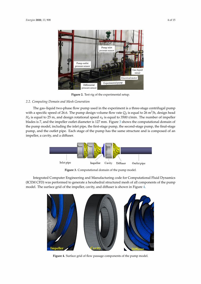
Integrated Computer Engineering and Manufacturing code for Computational Fluid Dynamics (ICEM CFD) was performed to generate a hexahedral structured mesh of all components of the pump model. The surface grid of the impeller, cavity, and diffuser is shown in Figure 4.

Figure 4. Surface grid of flow passage components of the pump model.

Figure 2. Test rig of the experimental setup.

2.2. Computing Domain and Mesh Generation

The gas–liquid two-phase flow pump used in the experiment is a three-stage centrifugal pumpwith a specific speed of 26.6. The pump design volume flow rate Qd is equal to 26 m3/h, design headHd is equal to 25 m, and design rotational speed nd is equal to 3500 r/min. The number of impellerblades is 7, and the impeller outlet diameter is 127 mm. Figure 3 shows the computational domain ofthe pump model, including the inlet pipe, the first-stage pump, the second-stage pump, the final-stagepump, and the outlet pipe. Each stage of the pump has the same structure and is composed of animpeller, a cavity, and a diffuser.

Energies 2020, 13, x FOR PEER REVIEW 4 of 15

Figure 2. Test rig of the experimental setup.

2.2. Computing Domain and Mesh Generation

The gas–liquid two-phase flow pump used in the experiment is a three-stage centrifugal pump with a specific speed of 26.6. The pump design volume flow rate Qd is equal to 26 m3/h, design head Hd is equal to 25 m, and design rotational speed nd is equal to 3500 r/min. The number of impeller blades is 7, and the impeller outlet diameter is 127 mm. Figure 3 shows the computational domain of the pump model, including the inlet pipe, the first-stage pump, the second-stage pump, the final-stage pump, and the outlet pipe. Each stage of the pump has the same structure and is composed of an impeller, a cavity, and a diffuser.

Figure 3. Computational domain of the pump model.

Integrated Computer Engineering and Manufacturing code for Computational Fluid Dynamics (ICEM CFD) was performed to generate a hexahedral structured mesh of all components of the pump model. The surface grid of the impeller, cavity, and diffuser is shown in Figure 4.

Figure 4. Surface grid of flow passage components of the pump model.

Figure 3. Computational domain of the pump model.

Integrated Computer Engineering and Manufacturing code for Computational Fluid Dynamics(ICEM CFD) was performed to generate a hexahedral structured mesh of all components of the pumpmodel. The surface grid of the impeller, cavity, and diffuser is shown in Figure 4.

Energies 2020, 13, x FOR PEER REVIEW 4 of 15

Figure 2. Test rig of the experimental setup.

2.2. Computing Domain and Mesh Generation

The gas–liquid two-phase flow pump used in the experiment is a three-stage centrifugal pump with a specific speed of 26.6. The pump design volume flow rate Qd is equal to 26 m3/h, design head Hd is equal to 25 m, and design rotational speed nd is equal to 3500 r/min. The number of impeller blades is 7, and the impeller outlet diameter is 127 mm. Figure 3 shows the computational domain of the pump model, including the inlet pipe, the first-stage pump, the second-stage pump, the final-stage pump, and the outlet pipe. Each stage of the pump has the same structure and is composed of an impeller, a cavity, and a diffuser.

Figure 3. Computational domain of the pump model.

Integrated Computer Engineering and Manufacturing code for Computational Fluid Dynamics (ICEM CFD) was performed to generate a hexahedral structured mesh of all components of the pump model. The surface grid of the impeller, cavity, and diffuser is shown in Figure 4.

Figure 4. Surface grid of flow passage components of the pump model. Figure 4. Surface grid of flow passage components of the pump model.

Energies 2020, 13, 908 5 of 15

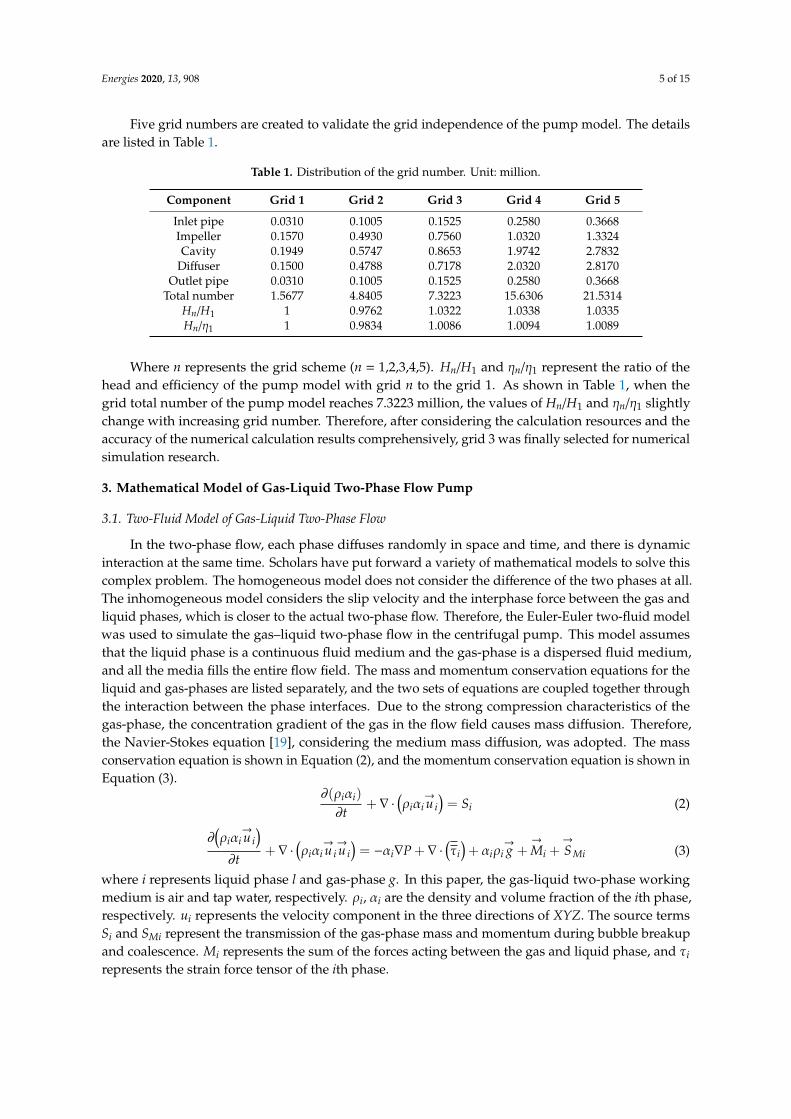
Five grid numbers are created to validate the grid independence of the pump model. The detailsare listed in Table 1.

Table 1. Distribution of the grid number. Unit: million.

Component Grid 1 Grid 2 Grid 3 Grid 4 Grid 5

Inlet pipe 0.0310 0.1005 0.1525 0.2580 0.3668Impeller 0.1570 0.4930 0.7560 1.0320 1.3324Cavity 0.1949 0.5747 0.8653 1.9742 2.7832

Diffuser 0.1500 0.4788 0.7178 2.0320 2.8170Outlet pipe 0.0310 0.1005 0.1525 0.2580 0.3668

Total number 1.5677 4.8405 7.3223 15.6306 21.5314Hn/H1 1 0.9762 1.0322 1.0338 1.0335Hn/η1 1 0.9834 1.0086 1.0094 1.0089

Where n represents the grid scheme (n = 1,2,3,4,5). Hn/H1 and ηn/η1 represent the ratio of thehead and efficiency of the pump model with grid n to the grid 1. As shown in Table 1, when thegrid total number of the pump model reaches 7.3223 million, the values of Hn/H1 and ηn/η1 slightlychange with increasing grid number. Therefore, after considering the calculation resources and theaccuracy of the numerical calculation results comprehensively, grid 3 was finally selected for numericalsimulation research.

3. Mathematical Model of Gas-Liquid Two-Phase Flow Pump

3.1. Two-Fluid Model of Gas-Liquid Two-Phase Flow

In the two-phase flow, each phase diffuses randomly in space and time, and there is dynamicinteraction at the same time. Scholars have put forward a variety of mathematical models to solve thiscomplex problem. The homogeneous model does not consider the difference of the two phases at all.The inhomogeneous model considers the slip velocity and the interphase force between the gas andliquid phases, which is closer to the actual two-phase flow. Therefore, the Euler-Euler two-fluid modelwas used to simulate the gas–liquid two-phase flow in the centrifugal pump. This model assumesthat the liquid phase is a continuous fluid medium and the gas-phase is a dispersed fluid medium,and all the media fills the entire flow field. The mass and momentum conservation equations for theliquid and gas-phases are listed separately, and the two sets of equations are coupled together throughthe interaction between the phase interfaces. Due to the strong compression characteristics of thegas-phase, the concentration gradient of the gas in the flow field causes mass diffusion. Therefore,the Navier-Stokes equation [19], considering the medium mass diffusion, was adopted. The massconservation equation is shown in Equation (2), and the momentum conservation equation is shown inEquation (3).

∂(ρiαi)

∂t+∇ ·

(ρiαi

→u i

)= Si (2)

∂(ρiαi

→u i

)∂t

+∇ ·(ρiαi

→u i→u i

)= −αi∇P +∇ ·

(τi)+ αiρi

→g +

→

Mi +→

SMi (3)

where i represents liquid phase l and gas-phase g. In this paper, the gas-liquid two-phase workingmedium is air and tap water, respectively. ρi, αi are the density and volume fraction of the ith phase,respectively. ui represents the velocity component in the three directions of XYZ. The source termsSi and SMi represent the transmission of the gas-phase mass and momentum during bubble breakupand coalescence. Mi represents the sum of the forces acting between the gas and liquid phase, and τirepresents the strain force tensor of the ith phase.

Energies 2020, 13, 908 6 of 15

3.2. Discrete Particle Population Balance Model (PBM)

Discrete PBM was used to simulate the distribution of the number and size of bubbles in the flowfield. This model considers the breakup and aggregation of bubbles due to the forces between thegas and liquid phases. The bubble breakup model used was the Luo and Svendsen model [22], andthe bubble coalescence model used was the Prince and Blanch model [23]. The mass transfer Si of thegas-phase can be obtained from Equation (4):

Sg = BB −DB + BC −DC (4)

where BB, DB, BC, and DC, respectively, represent the bubble birth rates due to the breakup of largerparticles, the bubble death rate due to the breakup of larger particles, the bubble birth rate due tocoalescence of smaller particles, and the bubble death rate due to the coalescence of smaller particles.

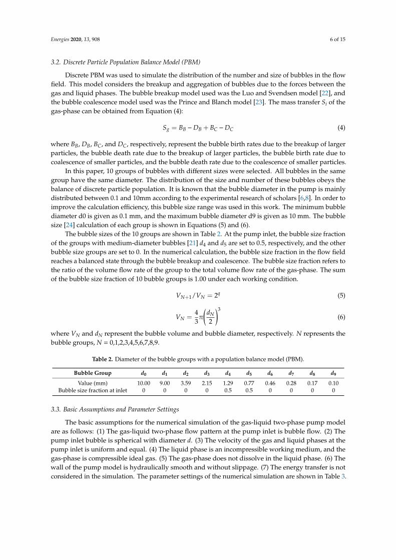
In this paper, 10 groups of bubbles with different sizes were selected. All bubbles in the samegroup have the same diameter. The distribution of the size and number of these bubbles obeys thebalance of discrete particle population. It is known that the bubble diameter in the pump is mainlydistributed between 0.1 and 10mm according to the experimental research of scholars [6,8]. In order toimprove the calculation efficiency, this bubble size range was used in this work. The minimum bubblediameter d0 is given as 0.1 mm, and the maximum bubble diameter d9 is given as 10 mm. The bubblesize [24] calculation of each group is shown in Equations (5) and (6).

The bubble sizes of the 10 groups are shown in Table 2. At the pump inlet, the bubble size fractionof the groups with medium-diameter bubbles [21] d4 and d5 are set to 0.5, respectively, and the otherbubble size groups are set to 0. In the numerical calculation, the bubble size fraction in the flow fieldreaches a balanced state through the bubble breakup and coalescence. The bubble size fraction refers tothe ratio of the volume flow rate of the group to the total volume flow rate of the gas-phase. The sumof the bubble size fraction of 10 bubble groups is 1.00 under each working condition.

VN+1/VN = 2q (5)

VN =43π

(dN

2

)3

(6)

where VN and dN represent the bubble volume and bubble diameter, respectively. N represents thebubble groups, N = 0,1,2,3,4,5,6,7,8,9.

Table 2. Diameter of the bubble groups with a population balance model (PBM).

Bubble Group d0 d1 d2 d3 d4 d5 d6 d7 d8 d9

Value (mm) 10.00 9.00 3.59 2.15 1.29 0.77 0.46 0.28 0.17 0.10Bubble size fraction at inlet 0 0 0 0 0.5 0.5 0 0 0 0

3.3. Basic Assumptions and Parameter Settings

The basic assumptions for the numerical simulation of the gas-liquid two-phase pump modelare as follows: (1) The gas-liquid two-phase flow pattern at the pump inlet is bubble flow. (2) Thepump inlet bubble is spherical with diameter d. (3) The velocity of the gas and liquid phases at thepump inlet is uniform and equal. (4) The liquid phase is an incompressible working medium, and thegas-phase is compressible ideal gas. (5) The gas-phase does not dissolve in the liquid phase. (6) Thewall of the pump model is hydraulically smooth and without slippage. (7) The energy transfer is notconsidered in the simulation. The parameter settings of the numerical simulation are shown in Table 3.

Energies 2020, 13, 908 7 of 15

Table 3. Parameter setting for numerical simulation.

Setting Item Two-Phase Flow Parameters

Working medium Liquid-phase: water, ρ = 997 kg/m3

Gas-phase: air ideal gas

Inlet Boundary conditions Given high-pressure inletGiven inlet gas volume fraction (IGVF), λg

Outlet Boundary conditions Water mass flow rate: 7.2 kg/s

Rotational speed 3500 r/min

Turbulence model Liquid-phase: SST k-ω turbulence modelGas-phase: zero equation model

Gas–liquid two-phase

Homogeneous coupled with particle model, d = 0.1 mmInhomogeneous coupled with particle model, d = 0.1 mm

and 0.2 mm, respectivelyInhomogeneous model coupled with PBM

4. Results and Analysis

4.1. Experimental Validation

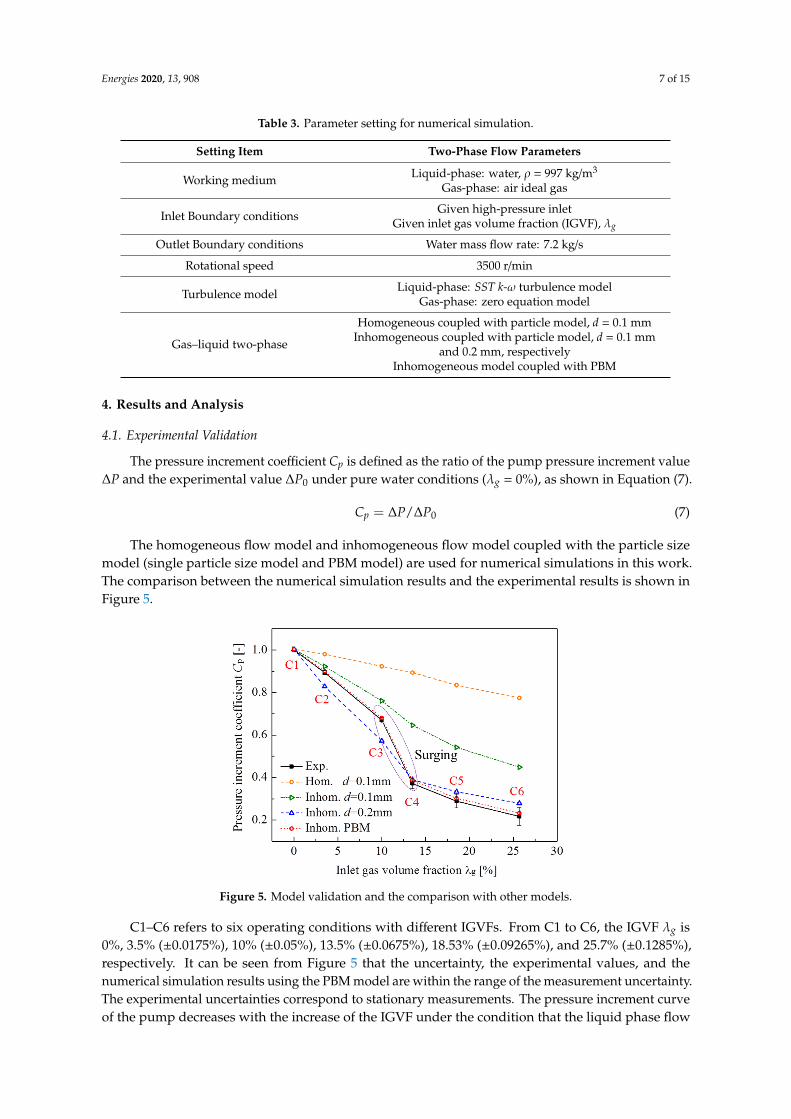
The pressure increment coefficient Cp is defined as the ratio of the pump pressure increment value∆P and the experimental value ∆P0 under pure water conditions (λg = 0%), as shown in Equation (7).

Cp = ∆P/∆P0 (7)

The homogeneous flow model and inhomogeneous flow model coupled with the particle sizemodel (single particle size model and PBM model) are used for numerical simulations in this work.The comparison between the numerical simulation results and the experimental results is shown inFigure 5.Energies 2020, 13, x FOR PEER REVIEW 8 of 15

Figure 5. Model validation and the comparison with other models.

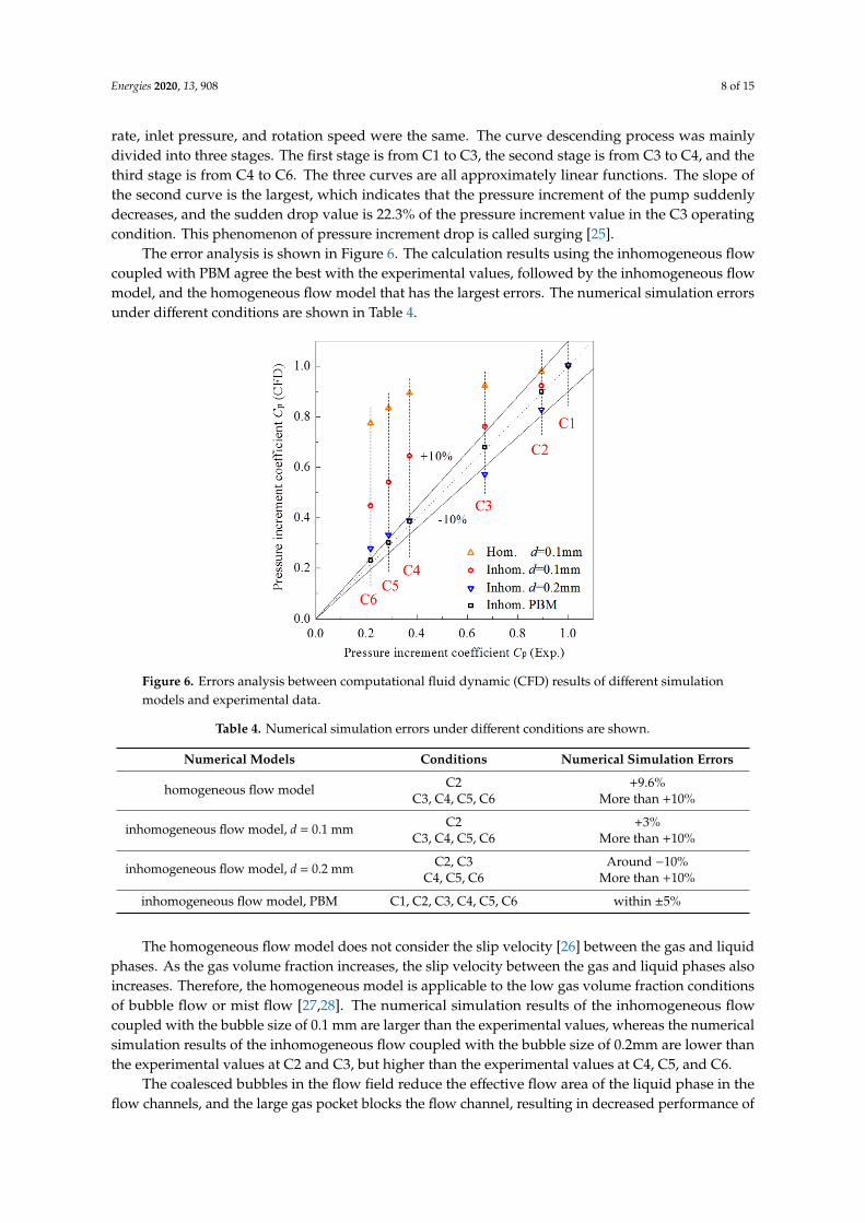
The error analysis is shown in Figure 6. The calculation results using the inhomogeneous flow coupled with PBM agree the best with the experimental values, followed by the inhomogeneous flow model, and the homogeneous flow model that has the largest errors. The numerical simulation errors under different conditions are shown in Table 4.

The homogeneous flow model does not consider the slip velocity [26] between the gas and liquid phases. As the gas volume fraction increases, the slip velocity between the gas and liquid phases also increases. Therefore, the homogeneous model is applicable to the low gas volume fraction conditions of bubble flow or mist flow [27,28]. The numerical simulation results of the inhomogeneous flow coupled with the bubble size of 0.1 mm are larger than the experimental values, whereas the numerical simulation results of the inhomogeneous flow coupled with the bubble size of 0.2mm are lower than the experimental values at C2 and C3, but higher than the experimental values at C4, C5, and C6.

Figure 6. Errors analysis between computational fluid dynamic (CFD) results of different simulation models and experimental data.

Figure 5. Model validation and the comparison with other models.

C1–C6 refers to six operating conditions with different IGVFs. From C1 to C6, the IGVF λg is0%, 3.5% (±0.0175%), 10% (±0.05%), 13.5% (±0.0675%), 18.53% (±0.09265%), and 25.7% (±0.1285%),respectively. It can be seen from Figure 5 that the uncertainty, the experimental values, and thenumerical simulation results using the PBM model are within the range of the measurement uncertainty.The experimental uncertainties correspond to stationary measurements. The pressure increment curveof the pump decreases with the increase of the IGVF under the condition that the liquid phase flow

Energies 2020, 13, 908 8 of 15

rate, inlet pressure, and rotation speed were the same. The curve descending process was mainlydivided into three stages. The first stage is from C1 to C3, the second stage is from C3 to C4, and thethird stage is from C4 to C6. The three curves are all approximately linear functions. The slope ofthe second curve is the largest, which indicates that the pressure increment of the pump suddenlydecreases, and the sudden drop value is 22.3% of the pressure increment value in the C3 operatingcondition. This phenomenon of pressure increment drop is called surging [25].

The error analysis is shown in Figure 6. The calculation results using the inhomogeneous flowcoupled with PBM agree the best with the experimental values, followed by the inhomogeneous flowmodel, and the homogeneous flow model that has the largest errors. The numerical simulation errorsunder different conditions are shown in Table 4.

Energies 2020, 13, x FOR PEER REVIEW 8 of 15

Figure 5. Model validation and the comparison with other models.

The error analysis is shown in Figure 6. The calculation results using the inhomogeneous flow coupled with PBM agree the best with the experimental values, followed by the inhomogeneous flow model, and the homogeneous flow model that has the largest errors. The numerical simulation errors under different conditions are shown in Table 4.

The homogeneous flow model does not consider the slip velocity [26] between the gas and liquid phases. As the gas volume fraction increases, the slip velocity between the gas and liquid phases also increases. Therefore, the homogeneous model is applicable to the low gas volume fraction conditions of bubble flow or mist flow [27,28]. The numerical simulation results of the inhomogeneous flow coupled with the bubble size of 0.1 mm are larger than the experimental values, whereas the numerical simulation results of the inhomogeneous flow coupled with the bubble size of 0.2mm are lower than the experimental values at C2 and C3, but higher than the experimental values at C4, C5, and C6.

Figure 6. Errors analysis between computational fluid dynamic (CFD) results of different simulation models and experimental data.

Figure 6. Errors analysis between computational fluid dynamic (CFD) results of different simulationmodels and experimental data.

Table 4. Numerical simulation errors under different conditions are shown.

Numerical Models Conditions Numerical Simulation Errors

homogeneous flow model C2 +9.6%C3, C4, C5, C6 More than +10%

inhomogeneous flow model, d = 0.1 mm C2 +3%C3, C4, C5, C6 More than +10%

inhomogeneous flow model, d = 0.2 mm C2, C3 Around −10%C4, C5, C6 More than +10%

inhomogeneous flow model, PBM C1, C2, C3, C4, C5, C6 within ±5%

The homogeneous flow model does not consider the slip velocity [26] between the gas and liquidphases. As the gas volume fraction increases, the slip velocity between the gas and liquid phases alsoincreases. Therefore, the homogeneous model is applicable to the low gas volume fraction conditionsof bubble flow or mist flow [27,28]. The numerical simulation results of the inhomogeneous flowcoupled with the bubble size of 0.1 mm are larger than the experimental values, whereas the numericalsimulation results of the inhomogeneous flow coupled with the bubble size of 0.2mm are lower thanthe experimental values at C2 and C3, but higher than the experimental values at C4, C5, and C6.

The coalesced bubbles in the flow field reduce the effective flow area of the liquid phase in theflow channels, and the large gas pocket blocks the flow channel, resulting in decreased performance of

Energies 2020, 13, 908 9 of 15

the pump. The probability of bubble coalescence into large bubbles increases with increasing bubblediameter and gas volume fraction. Therefore, when using a single-bubble size model, the initial bubblesize d needs to be reset as the operating conditions change [29–31].

In the gas-liquid two-phase flow field, the bubble size distribution in the gas–liquid two-phaseflow changes with the occurrence of multiphase system reactions and transfer phenomena, and thecoalescence and fragmentation between the bubbles cause the particle size to change. The PBM canmake up for the shortcomings of the single-bubble size model well. There are three main characteristicsof the PBM: (1) Multiple groups of bubble diameters are set, as shown in Table 2, and the mass transfer,break up, and coalescence between bubbles are considered. (2) Various bubble sizes coexist and thenumbers are balanced with each other. (3) Under small gas volume fraction conditions, large bubblesare broken into small ones, which then coalesce into large particles under large gas volume fractionconditions until the particle group reaches a balanced state.

4.2. Internal Flow Field Analysis

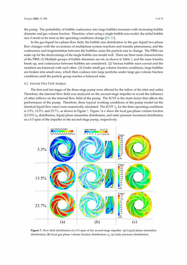
The first and last stages of the three-stage pump were affected by the inflow of the inlet and outlet.Therefore, the internal flow field was analyzed on the second-stage impeller to avoid the influenceof other inflows on the internal flow field of the pump. The IGVF is the main factor that affects theperformance of the pump. Therefore, three typical working conditions of the pump model (at theidentical liquid flow rates) were numerically simulated. The IGVF λg for the three operating conditionsis 3.5%, 13.5%, and 25.7%, as shown in Figure 7. Figure 7a–c show the local gas-phase volume fraction(LGVF) αg distribution, liquid phase streamline distribution, and static pressure increment distributionat a 0.5 span of the impeller in the second-stage pump, respectively.Energies 2020, 13, x FOR PEER REVIEW 10 of 15

Figure 7. Flow field distribution at a 0.5 span of the second-stage impeller. (a) Liquid phase streamline distribution; (b) local gas-phase volume fraction distribution αg; (c) static pressure distribution.

As shown in Figure 7a, the gas-phase in the impeller flow channel is mainly distributed near the suction surface (SS) of the blade leading edge under low IGVF conditions, and it diffuses to the PS of the blade and downstream of the flow channel as the IGVF increases. There are three main reasons for the gas-phase separation and why it is stuck near the SS of the impeller blade: (1) The gas and liquid exhibit flow velocity separation at the blade inlet, as shown in Figure 7b. The flow direction of the liquid phase at the inlet of the blade is mainly from the SS to the PS of the blade. Due to the low density of gas-phase, it obtains less energy from the impeller blades, resulting in its velocity being lower than that of the liquid phase, which causes the gas-phase to stay at the leading edge of the blade SS. (2) The high-pressure and high velocity fluid near the outlet of the blade PS flows towards the SS of the same blade generating a jet region and a vortex region in an anticlockwise direction. The jet flows towards the outlet of the impeller while taking away the bubbles near the outlet of the impeller. This vortex is located inside of the jet region, as shown by the black arrow line in Figure 7b. The vortex region blocks the fluid near the suction surface, forms a backflow and vortex, and prevents the bubbles from flowing out of the impeller. (3) Comparing Figure 7a and 7b, it can be seen that under the condition of high IGVF, the region with high LGVF near the suction surface corresponds to the liquid vortex and low velocity recirculation zone, as shown by the red arrow line in Figure 7b. In this region, the relative velocity direction of the liquid phase is directed from the impeller outlet to the inlet, and the drag force of the bubble is directed to the impeller inlet along the liquid streamline. Therefore, it is difficult for the bubbles to be carried away from the impeller channel by the liquid, causing the gas to aggregate at the liquid phase vortex and gas–liquid separation.

As shown in Figure 7c, the pressure increment value of static pressure increases uniformly in the radial direction from the impeller inlet to the impeller outlet under low IGVF conditions. Under high IGVF conditions, a reverse pressure gradient zone is generated near the blade PS of the downstream impeller flow channel. The pressure increment value is almost unchanged within 0.7 times the relative radius of the impeller and the value increases slightly near the outlet of the impeller.

Figure 7. Flow field distribution at a 0.5 span of the second-stage impeller. (a) Liquid phase streamlinedistribution; (b) local gas-phase volume fraction distribution αg; (c) static pressure distribution.

Energies 2020, 13, 908 10 of 15

It shows that with the increase of IGVF, the flow field distribution in the impeller changesdrastically, especially from the IGVF of 3.5% to 13.5%. The flow loss is the largest at this stage, and theexternal characteristics of the pump drop suddenly (as shown in Figure 5).

At high IGVF conditions, the area with high LGVF near the suction surface also increases,indicating that the gas-phase has accumulated and stuck on the suction surface. At the same time,it can be seen that the accumulation of gas-phase makes the liquid flow space be severely squeezed,which causes the relative velocity of the liquid phase near the pressure surface (PS) of the blade toincrease significantly, and leading to large flow losses in the pump.

As shown in Figure 7a, the gas-phase in the impeller flow channel is mainly distributed near thesuction surface (SS) of the blade leading edge under low IGVF conditions, and it diffuses to the PS ofthe blade and downstream of the flow channel as the IGVF increases. There are three main reasons forthe gas-phase separation and why it is stuck near the SS of the impeller blade: (1) The gas and liquidexhibit flow velocity separation at the blade inlet, as shown in Figure 7b. The flow direction of theliquid phase at the inlet of the blade is mainly from the SS to the PS of the blade. Due to the low densityof gas-phase, it obtains less energy from the impeller blades, resulting in its velocity being lower thanthat of the liquid phase, which causes the gas-phase to stay at the leading edge of the blade SS. (2) Thehigh-pressure and high velocity fluid near the outlet of the blade PS flows towards the SS of the sameblade generating a jet region and a vortex region in an anticlockwise direction. The jet flows towardsthe outlet of the impeller while taking away the bubbles near the outlet of the impeller. This vortex islocated inside of the jet region, as shown by the black arrow line in Figure 7b. The vortex region blocksthe fluid near the suction surface, forms a backflow and vortex, and prevents the bubbles from flowingout of the impeller. (3) Comparing Figure 7a and 7b, it can be seen that under the condition of highIGVF, the region with high LGVF near the suction surface corresponds to the liquid vortex and lowvelocity recirculation zone, as shown by the red arrow line in Figure 7b. In this region, the relativevelocity direction of the liquid phase is directed from the impeller outlet to the inlet, and the drag forceof the bubble is directed to the impeller inlet along the liquid streamline. Therefore, it is difficult forthe bubbles to be carried away from the impeller channel by the liquid, causing the gas to aggregate atthe liquid phase vortex and gas–liquid separation.

As shown in Figure 7c, the pressure increment value of static pressure increases uniformly in theradial direction from the impeller inlet to the impeller outlet under low IGVF conditions. Under highIGVF conditions, a reverse pressure gradient zone is generated near the blade PS of the downstreamimpeller flow channel. The pressure increment value is almost unchanged within 0.7 times the relativeradius of the impeller and the value increases slightly near the outlet of the impeller. The main reasonfor the uneven pressure distribution is that there is a large amount of gas accumulation in the flowchannel under high IGVF conditions, and the energy applied by the impeller to the fluid is dissipatedby the backflow. Therefore, the pressurized area is mainly concentrated downstream of the impellerflow channel, and the value of pressure increment decreases rapidly with the increase of the IGVF.

4.3. Distribution of Bubbles with Different Particle Sizes in the Pump

The numerical simulation results of the discrete particle population balance model were analyzedto understand the distribution of bubbles with different particle sizes in the pump under differentoperating conditions. The bubble size fraction of 10 bubble groups (Table 2) at a 0.5 span of the pumpimpeller and guide vane is shown in Figure 8.

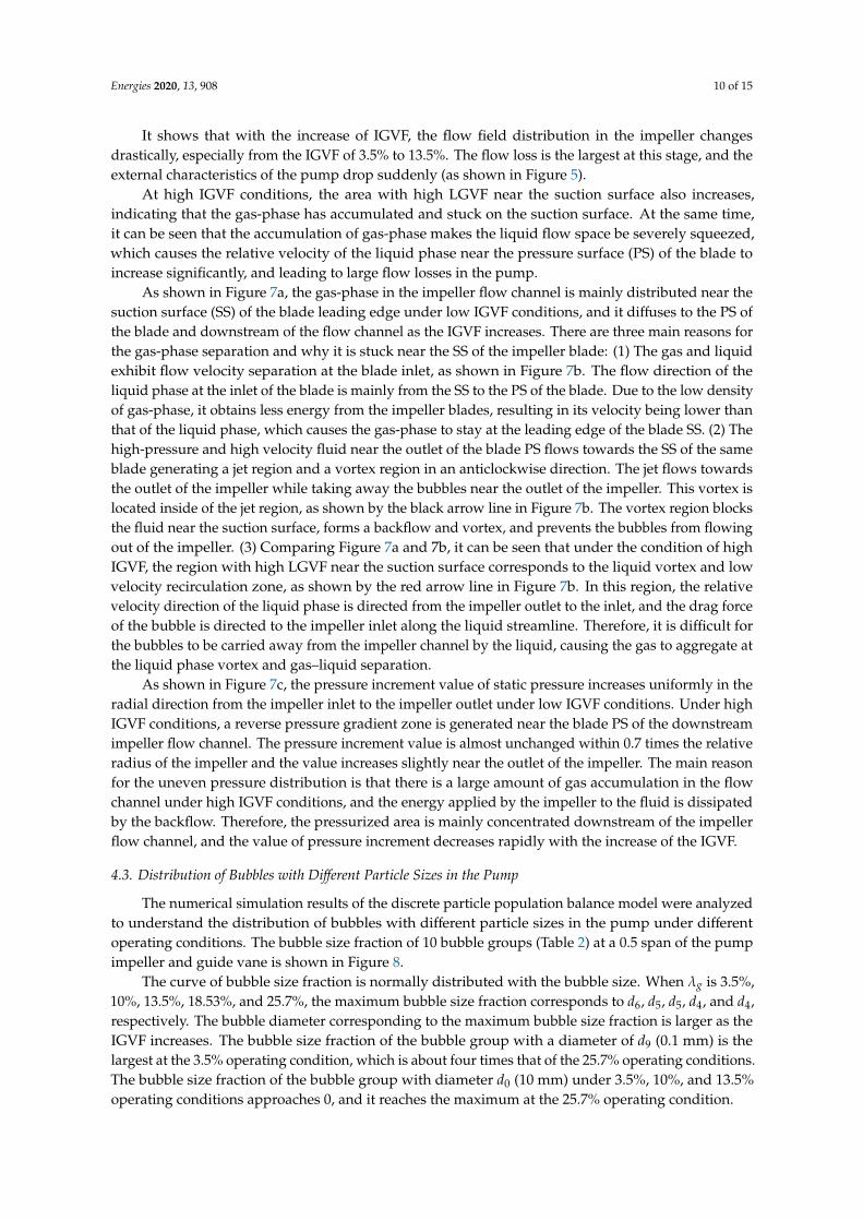
The curve of bubble size fraction is normally distributed with the bubble size. When λg is 3.5%,10%, 13.5%, 18.53%, and 25.7%, the maximum bubble size fraction corresponds to d6, d5, d5, d4, and d4,respectively. The bubble diameter corresponding to the maximum bubble size fraction is larger as theIGVF increases. The bubble size fraction of the bubble group with a diameter of d9 (0.1 mm) is thelargest at the 3.5% operating condition, which is about four times that of the 25.7% operating conditions.The bubble size fraction of the bubble group with diameter d0 (10 mm) under 3.5%, 10%, and 13.5%operating conditions approaches 0, and it reaches the maximum at the 25.7% operating condition.

Energies 2020, 13, 908 11 of 15

Considering that the bubble size fraction of both the d4 and d5 bubble groups at the pump inletis 0.5, the bubbles with the size of d4 and d5 in the flow field are assumed to be neither broken norcoalesced. The bubble size fraction with neither broken nor coalesced bubbles is shown by the curvebetween the two black dotted lines in Figure 8. The curve on the left side of the black dotted lineindicates the bubble size fraction of broken bubbles with diameters smaller than d5, and the curve onthe right side of the black dashed line represents the bubble size fraction of the coalesced bubbles withdiameters larger than d4. Under different IGVF conditions, the value of bubble size fraction at theareas of broken bubbles and coalescence bubbles is shown in Table 5. It shows that the bubbles tend tobreak from large to small bubbles under small IGVFs while coalesce from small to large bubbles underlarge IGVFs.

Energies 2020, 13, x FOR PEER REVIEW 11 of 15

The main reason for the uneven pressure distribution is that there is a large amount of gas accumulation in the flow channel under high IGVF conditions, and the energy applied by the impeller to the fluid is dissipated by the backflow. Therefore, the pressurized area is mainly concentrated downstream of the impeller flow channel, and the value of pressure increment decreases rapidly with the increase of the IGVF.

4.3. Distribution of Bubbles with Different Particle Sizes in the Pump

The numerical simulation results of the discrete particle population balance model were analyzed to understand the distribution of bubbles with different particle sizes in the pump under different operating conditions. The bubble size fraction of 10 bubble groups (Table 2) at a 0.5 span of the pump impeller and guide vane is shown in Figure 8.

The curve of bubble size fraction is normally distributed with the bubble size. When λg is 3.5%, 10%, 13.5%, 18.53%, and 25.7%, the maximum bubble size fraction corresponds to d6, d5, d5, d4, and d4, respectively. The bubble diameter corresponding to the maximum bubble size fraction is larger as the IGVF increases. The bubble size fraction of the bubble group with a diameter of d9 (0.1 mm) is the largest at the 3.5% operating condition, which is about four times that of the 25.7% operating conditions. The bubble size fraction of the bubble group with diameter d0 (10 mm) under 3.5%, 10%, and 13.5% operating conditions approaches 0, and it reaches the maximum at the 25.7% operating condition.

Considering that the bubble size fraction of both the d4 and d5 bubble groups at the pump inlet is 0.5, the bubbles with the size of d4 and d5 in the flow field are assumed to be neither broken nor coalesced. The bubble size fraction with neither broken nor coalesced bubbles is shown by the curve between the two black dotted lines in Figure 8. The curve on the left side of the black dotted line indicates the bubble size fraction of broken bubbles with diameters smaller than d5, and the curve on the right side of the black dashed line represents the bubble size fraction of the coalesced bubbles with diameters larger than d4. Under different IGVF conditions, the value of bubble size fraction at the areas of broken bubbles and coalescence bubbles is shown in Table 5. It shows that the bubbles tend to break from large to small bubbles under small IGVFs while coalesce from small to large bubbles under large IGVFs.

Figure 8. Bubble size fraction at a 0.5 span of the pump impeller and guide vane at different IGVF operating conditions.

Table 5. The value of bubble size fraction at different conditions.

Areas IGVF = 3.5% IGVF = 10% IGVF = 25.7% The area of broken bubbles the highest the middle the lowest

The area of bubble coalescences the lowest the middle the highest

Figure 8. Bubble size fraction at a 0.5 span of the pump impeller and guide vane at different IGVFoperating conditions.

Table 5. The value of bubble size fraction at different conditions.

Areas IGVF = 3.5% IGVF = 10% IGVF = 25.7%

The area of broken bubbles the highest the middle the lowestThe area of bubble coalescences the lowest the middle the highest

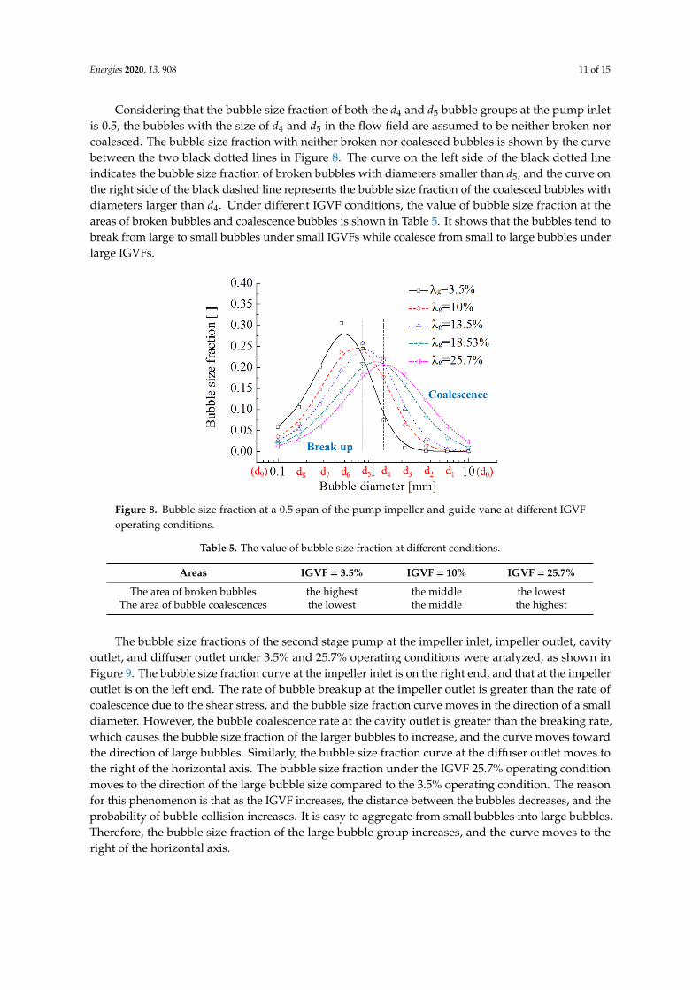
The bubble size fractions of the second stage pump at the impeller inlet, impeller outlet, cavityoutlet, and diffuser outlet under 3.5% and 25.7% operating conditions were analyzed, as shown inFigure 9. The bubble size fraction curve at the impeller inlet is on the right end, and that at the impelleroutlet is on the left end. The rate of bubble breakup at the impeller outlet is greater than the rate ofcoalescence due to the shear stress, and the bubble size fraction curve moves in the direction of a smalldiameter. However, the bubble coalescence rate at the cavity outlet is greater than the breaking rate,which causes the bubble size fraction of the larger bubbles to increase, and the curve moves towardthe direction of large bubbles. Similarly, the bubble size fraction curve at the diffuser outlet moves tothe right of the horizontal axis. The bubble size fraction under the IGVF 25.7% operating conditionmoves to the direction of the large bubble size compared to the 3.5% operating condition. The reasonfor this phenomenon is that as the IGVF increases, the distance between the bubbles decreases, and theprobability of bubble collision increases. It is easy to aggregate from small bubbles into large bubbles.Therefore, the bubble size fraction of the large bubble group increases, and the curve moves to theright of the horizontal axis.

Energies 2020, 13, 908 12 of 15

Energies 2020, 13, x FOR PEER REVIEW 12 of 15

The bubble size fractions of the second stage pump at the impeller inlet, impeller outlet, cavity outlet, and diffuser outlet under 3.5% and 25.7% operating conditions were analyzed, as shown in Figure 9. The bubble size fraction curve at the impeller inlet is on the right end, and that at the impeller outlet is on the left end. The rate of bubble breakup at the impeller outlet is greater than the rate of coalescence due to the shear stress, and the bubble size fraction curve moves in the direction of a small diameter. However, the bubble coalescence rate at the cavity outlet is greater than the breaking rate, which causes the bubble size fraction of the larger bubbles to increase, and the curve moves toward the direction of large bubbles. Similarly, the bubble size fraction curve at the diffuser outlet moves to the right of the horizontal axis. The bubble size fraction under the IGVF 25.7% operating condition moves to the direction of the large bubble size compared to the 3.5% operating condition. The reason for this phenomenon is that as the IGVF increases, the distance between the bubbles decreases, and the probability of bubble collision increases. It is easy to aggregate from small bubbles into large bubbles. Therefore, the bubble size fraction of the large bubble group increases, and the curve moves to the right of the horizontal axis.

(a) (b)

Figure 9. Bubble size distribution at the inlet and outlet of the 2nd-stage pump components. (a) λg = 3.5%; (b) λg = 25.7%.

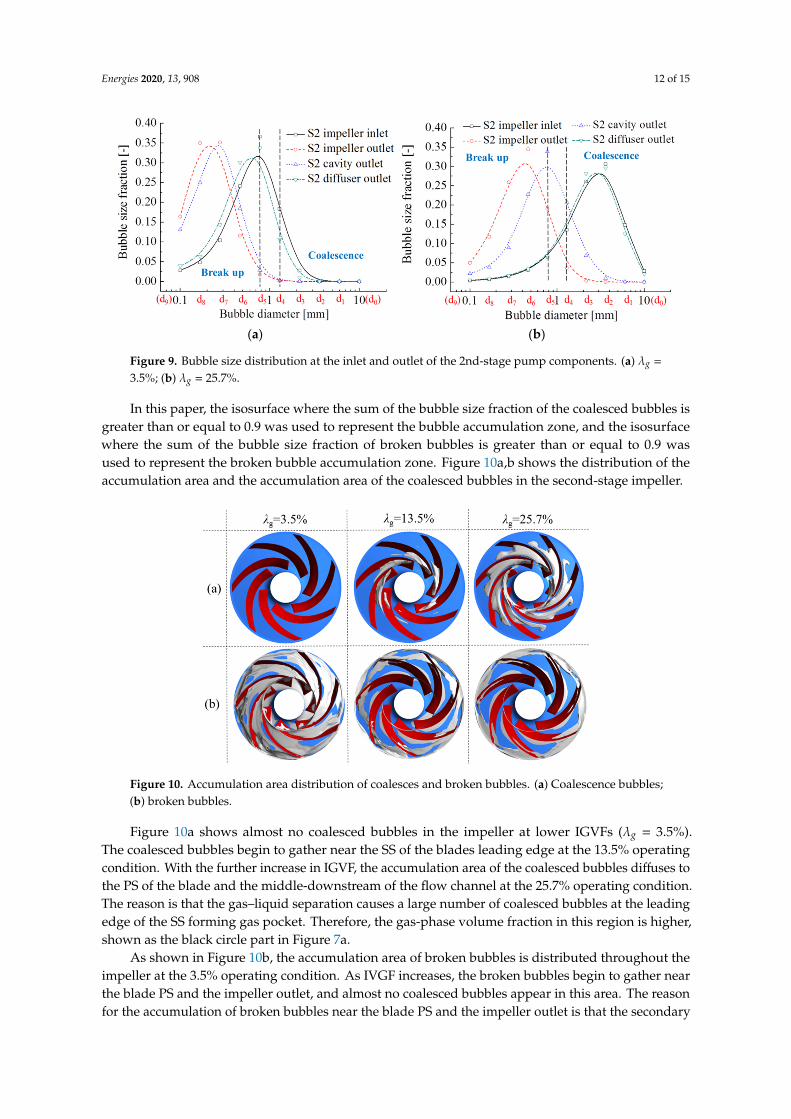
In this paper, the isosurface where the sum of the bubble size fraction of the coalesced bubbles is greater than or equal to 0.9 was used to represent the bubble accumulation zone, and the isosurface where the sum of the bubble size fraction of broken bubbles is greater than or equal to 0.9 was used to represent the broken bubble accumulation zone. Figure 10a,b shows the distribution of the accumulation area and the accumulation area of the coalesced bubbles in the second-stage impeller.

Figure 9. Bubble size distribution at the inlet and outlet of the 2nd-stage pump components. (a) λg =

3.5%; (b) λg = 25.7%.

In this paper, the isosurface where the sum of the bubble size fraction of the coalesced bubbles isgreater than or equal to 0.9 was used to represent the bubble accumulation zone, and the isosurfacewhere the sum of the bubble size fraction of broken bubbles is greater than or equal to 0.9 wasused to represent the broken bubble accumulation zone. Figure 10a,b shows the distribution of theaccumulation area and the accumulation area of the coalesced bubbles in the second-stage impeller.

Energies 2020, 13, x FOR PEER REVIEW 12 of 15

The bubble size fractions of the second stage pump at the impeller inlet, impeller outlet, cavity outlet, and diffuser outlet under 3.5% and 25.7% operating conditions were analyzed, as shown in Figure 9. The bubble size fraction curve at the impeller inlet is on the right end, and that at the impeller outlet is on the left end. The rate of bubble breakup at the impeller outlet is greater than the rate of coalescence due to the shear stress, and the bubble size fraction curve moves in the direction of a small diameter. However, the bubble coalescence rate at the cavity outlet is greater than the breaking rate, which causes the bubble size fraction of the larger bubbles to increase, and the curve moves toward the direction of large bubbles. Similarly, the bubble size fraction curve at the diffuser outlet moves to the right of the horizontal axis. The bubble size fraction under the IGVF 25.7% operating condition moves to the direction of the large bubble size compared to the 3.5% operating condition. The reason for this phenomenon is that as the IGVF increases, the distance between the bubbles decreases, and the probability of bubble collision increases. It is easy to aggregate from small bubbles into large bubbles. Therefore, the bubble size fraction of the large bubble group increases, and the curve moves to the right of the horizontal axis.

(a) (b)

Figure 9. Bubble size distribution at the inlet and outlet of the 2nd-stage pump components. (a) λg = 3.5%; (b) λg = 25.7%.

In this paper, the isosurface where the sum of the bubble size fraction of the coalesced bubbles is greater than or equal to 0.9 was used to represent the bubble accumulation zone, and the isosurface where the sum of the bubble size fraction of broken bubbles is greater than or equal to 0.9 was used to represent the broken bubble accumulation zone. Figure 10a,b shows the distribution of the accumulation area and the accumulation area of the coalesced bubbles in the second-stage impeller.

Figure 10. Accumulation area distribution of coalesces and broken bubbles. (a) Coalescence bubbles;(b) broken bubbles.

Figure 10a shows almost no coalesced bubbles in the impeller at lower IGVFs (λg = 3.5%).The coalesced bubbles begin to gather near the SS of the blades leading edge at the 13.5% operatingcondition. With the further increase in IGVF, the accumulation area of the coalesced bubbles diffuses tothe PS of the blade and the middle-downstream of the flow channel at the 25.7% operating condition.The reason is that the gas–liquid separation causes a large number of coalesced bubbles at the leadingedge of the SS forming gas pocket. Therefore, the gas-phase volume fraction in this region is higher,shown as the black circle part in Figure 7a.

As shown in Figure 10b, the accumulation area of broken bubbles is distributed throughout theimpeller at the 3.5% operating condition. As IVGF increases, the broken bubbles begin to gather nearthe blade PS and the impeller outlet, and almost no coalesced bubbles appear in this area. The reasonfor the accumulation of broken bubbles near the blade PS and the impeller outlet is that the secondary

Energies 2020, 13, 908 13 of 15

flow and jet phenomenon cause the turbulence intensity of the flow field to increase, and the shearstress on the bubble increases. As a result, the bubbles easily break into small bubbles and do noteasily coalesce into larger ones. The location of the broken bubble distribution area corresponds to thesecondary flow and jet area. The small bubbles tend to flow out of the impeller due to the drag force ofwater, and the volume fraction of the gas-phase in this area is lower, shown as the red circle part inFigure 7a.

5. Conclusions

Experiments and numerical simulations of a gas-liquid two-phase three-stage centrifugal pumpwere conducted. The following conclusions were obtained:

(1) The Euler-Euler inhomogeneous flow coupled discrete particle population balance model wasapplied to a gas-liquid two-phase three-stage centrifugal pump. The maximal discrepancy between thenumerical simulation results and the experimental values is 5%, which verified the numerical model.

(2) The area with high LGVF diffuses from the suction of the blade leading edge toward the bladePS and downstream of the flow channel as the IGVF increases. The jet flow at the impeller outlet causesa liquid-phase vortex rotating counterclockwise. This vortex blocks the fluid on the suction surface,which results in the local vortices and backflow. The liquid phase vortex rotating clockwise and thebackflow near the SS trap the gas in the flow channel. Under high IGVF conditions, the pressurizedarea is mainly located at the downstream region of the impeller, and the pressurized value is very small.

(3) The average bubble size at the impeller outlet is the smallest, followed by the cavity outlet andthen the diffuser outlet, and the average bubble size at the impeller inlet is the largest.

(4) Bubbles tend to break into smaller bubbles under small IGVF conditions, while bubbles tend toaggregate into larger bubbles under large IGVF conditions. The lower the IGVF, the higher the bubblesize fraction of the broken bubbles, which mainly accumulate near the blade pressure surface and theimpeller outlet. And the higher the IGVF, the higher the bubble size fraction of the coalesced bubbles,which mainly accumulate near the SS of the blade leading edge and diffuse toward the blade PS andthe middle-downstream of the flow channel with the increase in IGVF.

This study provides a reference for the numerical simulation of gas-liquid two-phase flow inrotating machinery, and it helps for the design and optimization of gas-liquid two-phase flow centrifugalpumps through the research of bubble distribution.

Author Contributions: Numerical analysis and design of experiments were conducted by S.Y., S.S., X.L., S.C., C.L.and J.F. Analysis of the results of numerical simulation was conducted by S.Y. and S.S. S.Y. wrote the manuscriptwith revision by S.S. and X.L. All authors have read and agreed to the published version of the manuscript.

Funding: This research was supported by the National Natural Science Foundation of China (Grants Nos:51527808, 51839010, 51909212) and The Key Research and Development Program of Shaanxi Province in China(Grant Number: 2017ZDXM-GY-081).

Conflicts of Interest: The authors declare no conflict of interest.

Nomenclature

PBM Population balance modelλg Inlet gas volume fractionλl Inlet liquid volume fractionαg Local gas volume fractionQg gas volume flow rateQl liquid volume flow rateQd Pump design volume flow rateHd Pump design headnd Pump design rotational speedBB Bubble birth rates due to breakupDB Bubble death rate due to breakupBC Bubble birth rate due to coalescence

Energies 2020, 13, 908 14 of 15

DC Bubble death rate due to coalescenceVN Bubble volumedN Bubble diameter

References

1. Bagci, A.S.; Kece, M.; Nava, J. Challenges of using Electrical Submersible Pump (ESP) in high free gasapplications. In Proceedings of the CPS/SPE International Oil & Gas conference and Exhibition, Beijing,China, 8–10 June 2010; pp. 1–13.

2. Gupta, S.; Saputelli, L.; Corporation, F.; Nikolaou, M. Applying big data analytics to detect, diagnose, andprevent impending failures in Electric Submersible Pumps. In Proceedings of the SPE Annual TechnicalConference and Exhibition, Dubai, UAE, 26–28 September 2016; pp. 1–15.

3. Patil, A.; Gudigopuram, S.; Ayyildiz, B.; Delgado, A.; Morrison, G. Performance evaluation and dimensionalanalysis of multistage helicoaxial pump for two-phase flow. Int. J. Turbomach. Propuls. Power. 2019, 4, 22.[CrossRef]

4. Cardad, J.; Kenyery, F. CFD analysis of electric submersible pumps (ESP) handling two-phase mixtures.J. Energy Resour. Technol. 2004, 126, 99–104. [CrossRef]

5. Poullikkas, A. Effects of two-phase liquid-gas flow on the performance of nuclear reactor cooling pumps.Prog. Nucl. Energy. 2003, 42, 3–10. [CrossRef]

6. Verde, W.M.; Biazussi, J.L.; Sassim, N.A.; Bannwart, A.C. Experimental study of gas-liquid two-phase flowpatterns within centrifugal pumps impellers. Exp. Therm. Fluid Sci. 2017, 85, 37–51. [CrossRef]

7. Si, Q.R.; Bois, G.; Liao, M.Q.; Zhang, H.Y.; Cui, Q.L.; Yuan, S.Q. A comparative study on centrifugal pumpdesigns and two-phase flow characteristic under inlet gas entrainment conditions. Energies 2019, 13, 65.[CrossRef]

8. Zhang, J.Y.; Cai, S.J.; Li, Y.J.; Zhu, H.W.; Zhang, Y.X. Visualization study of gas-liquid two-phase flow patternsinside a three-stage rotodynamic multiphase pump. Exp. Therm. Fluid Sci. 2016, 70, 125–138. [CrossRef]

9. Paternost, G.M.; Bannwart, A.C.; Estevam, V. Experimental study of a centrifugal pump handling viscousfluid and two-phase flow. In Proceedings of the SPE Artificial Lift Conference, Cartagena, Colombia, 21–22May 2015; pp. 146–155.

10. Neumann, M.; Schafer, T.; Bieberle, A. An experimental study on the gas entrainment in horizontally andvertically installed centrifugal pumps. J. Fluids Eng. 2016, 9, 138. [CrossRef]

11. Xu, Y.; Cao, S.L.; Sano, T.; Wakai, T.; Reclari, M. Experimental investigation on transient pressure characteristicsin a helico-axial multiphase pump. Energies 2019, 12, 461. [CrossRef]

12. Pineda, H.; Biazussi, J.; López, F.; Oliveira, B.; Carvalho, R.D.M.; Bannwart, A.C.; Ratkovich, N. Phasedistribution analysis in an Electrical Submersible Pump (ESP) inlet handling water–air two-phase flow usingComputational Fluid Dynamics (CFD). J. Pet. Sci. Eng. 2016, 139, 49–61. [CrossRef]

13. Minemura, K.; Uchiyama, T. Three-dimensional calculation of air-water two-phase flow in centrifugal pumpimpeller based on a bubbly flow model. J. Fluids Eng. 1993, 115, 766–771. [CrossRef]

14. Si, Q.R.; Bois, G.; Jiang, Q.F.; He, W.T.; Ali, A. Yuan, S.Q. Investigation on the handling ability of centrifugalpumps under air–water two-phase inflow: model and experimental validation. Energies 2018, 11, 3048.[CrossRef]

15. Cardad, J.; Miguel, A.; Kenyery, F.; Tremante, A.; Aguillón, O. Characterization of a centrifugal pumpimpeller under two-phase flow conditions. J. Pet. Sci. Eng. 2008, 63, 18–22. [CrossRef]

16. Zhu, J.J.; Zhang, H.Q. Numerical study on electrical submersible pump two phase performance and bubblesize modeling. SPE Prod. Oper. 2017, 3, 32. [CrossRef]

17. Barrios, L. Visualization and Modeling of Multiphase Performance inside an Electrical Submersible Pump.Ph.D. Thesis, The University of Tulsa, Tulsa, OK, USA, 2007.

18. Gamboa, J. Prediction of the Transition in Two-Phase Performance of an Electrical Submersible Pump.Ph.D. Thesis, The University of Tulsa, Tulsa, OK, USA, 2008.

19. Frank, T.; Zwart, P.J.; Shi, J.; Krepper, E.; Lucas, D.; Rohde, U. Inhomogeneous MUSIG model-a populationbalance approach for polydispersed bubbly flows. In Proceedings of the International Conference NuclearEnergy for New Europe, Bled, Slovenia, 5–8 September 2005; pp. 1–14.

Energies 2020, 13, 908 15 of 15

20. Lilunnahar, D. Population Balance Modeling of Gas-Liquid Bubbly Flow: Capturing Colescence and BreakupProcesses. Ph.D. Thesis, RMIT University, Melbourne, Australia, 2014.

21. Chen, Y.M.; Patil, A.; Chen, Y.; Bai, C.R.; Wang, Y.T.; Morrison, G. Numerical study on the first stage headdegradation in an electrical submersible pump with population balance model. J. Energy Resour. Technol.2019, 141, 1–12. [CrossRef]

22. Luo, H.; Svendsen, H.F. Theoretical model for drop and bubble break-up in turbulent dispersion. AIChE J.1996, 42, 1225–1233. [CrossRef]

23. Prince, M.J.; Blanch, H.W. Bubble coalescence and break-up in air-sparged bubble columns. AIChE J. 1990,36, 1485–1499. [CrossRef]

24. Litster, J.D.; Smit, D.J.; Hounslow, M.J. Adjustable discretized population balance for growth and aggregation.AIChE J. 1995, 41, 591–603. [CrossRef]

25. Gamboa, J.; Prado, M. Review of electrical submersible pump surging correlation and models. SPE Prod.Oper. 2011, 26, 314–324. [CrossRef]

26. Caridad, J.; Kenyery, F. Slip factor for centrifugal impellers under single and two-phase flow conditions.J. Fluids Eng. 2005, 127, 317–321. [CrossRef]

27. Yu, Z.Y.; Zhu, B.S.; Cao, S.L.; Wang, G.Y. Application of two-fluid model in the unsteady flow simulation fora multiphase rotodynamic pump. In Proceedings of the 6th International Conference on Pumps and Fanswith Compressors and Wind Turbines, Beijing, China, 19–22 September 2013; Volume 52, pp. 1–8.

28. Zhu, J.J. Experiments, CFD Simulation and Modeling of ESP Performance under Gassy Conditions.Ph.D. Thesis, The University of Tulsa, Tulsa, OK, USA, 2017.

29. Zhu, J.J.; Zhang, H.Q. CFD Simulation of ESP Performance and Bubble Size Estimation under GassyConditions. In Proceedings of the SPE Annual Technical Conference and Exhibition, Amsterdam,The Netherlands, 27–29 October 2014; pp. 1–15.

30. Zhu, J.J.; Zhu, H.W.; Zhang, J.C.; Zhang, H.Q. A numerical study on flow patterns inside an electricalsubmersible pump (ESP) and comparison with visualization experiments. J. Pet. Sci. Eng. 2019, 173, 339–350.[CrossRef]

31. Izturiz, D.L. D_Lopez Effect of Bubble Size on an ESP Performance Handling Two-Phase Flow Conditions.Master’s Thesis, The Simon Bolivar University, Caracas, Venezuela, 2007.

© 2020 by the authors. Licensee MDPI, Basel, Switzerland. This article is an open accessarticle distributed under the terms and conditions of the Creative Commons Attribution(CC BY) license (http://creativecommons.org/licenses/by/4.0/).