explicit strong stability preserving multistage two-derivative
TRANSCRIPT
Explicit Strong Stability Preserving Multistage Two-DerivativeTime-Stepping Schemes
Andrew J. Christlieb1, Sigal Gottlieb2, Zachary Grant2∗, David C. Seal31Department of Computational Mathematics Science and Engineering, Department of Electrical Engineering,
and Department of Mathematics, Michigan State University2Department of Mathematics, University of Massachusetts, Dartmouth
3Department of Mathematics, U.S. Naval Academy.
Abstract
High order strong stability preserving (SSP) time discretizations are advantageous for use with spatial dis-cretizations with nonlinear stability properties for the solution of hyperbolic PDEs. The search for high orderstrong stability time-stepping methods with large allowable strong stability time-step has been an active area ofresearch over the last two decades. Recently, multiderivative time-stepping methods have been implemented withhyperbolic PDEs. In this work we describe sufficient conditions for a two-derivative multistage method to be SSP,and find some optimal SSP multistage two-derivative methods. While explicit SSP Runge–Kutta methods existonly up to fourth order, we show that this order barrier is broken for explicit multi-stage two-derivative methodsby designing a three stage fifth order SSP method. These methods are tested on simple scalar PDEs to verify theorder of convergence, and demonstrate the need for the SSP condition and the sharpness of the SSP time-step inmany cases.
1 Introduction1.1 SSP methodsWhen numerically approximating the solution to a hyperbolic conservation law of the form
Ut + f(U)x = 0, (1)
difficulties arise when the exact solution develops sharp gradients or discontinuities. Significant effort has beenexpended on developing spatial discretizations that can handle discontinuities [7], especially for high-order methods.These discretizations have special nonlinear non-inner-product stability properties, such as total variation stabilityor positivity, which ensure that when the semi-discretized equation
ut = F (u), (2)
(where u is a vector of approximations to U) is evolved using a forward Euler method, the numerical solutionsatisfies the desired strong stability property,
‖un + ∆tF (un)‖ ≤ ‖un‖, 0 ≤ ∆t ≤ ∆tFE , (3)
where ‖ · ‖ is any desired norm, semi-norm, or convex functional.In place of the first order time discretization (3), we typically require a higher-order time integrator, but we still
wish to ensure that the strong stability property ‖un+1‖ ≤ ‖un‖ is satisfied, perhaps under a modified time-steprestriction, where un is a discrete approximation to U at time tn. In [32] it was observed that some Runge–Kutta methods can be decomposed into convex combinations of forward Euler steps, so that any convex functional
∗Corresponding author: [email protected]
1
arX
iv:1
504.
0759
9v3
[m
ath.
NA
] 2
3 M
ar 2
016
property satisfied by (3) will be preserved by these higher-order time discretizations. For example, the s-stageexplicit Runge–Kutta method [33],
y(0) = un,
y(i) =
i−1∑j=0
(αi,jy
(j) + ∆tβi,jF (y(j))), i = 1, ..., s (4)
un+1 = y(s)
can be rewritten as convex combination of forward Euler steps of the form (3). If all the coefficients αi,j and βi,jare non-negative, and provided αi,j is zero only if its corresponding βi,j is zero, then each stage is bounded by
‖y(i)‖ =
∥∥∥∥∥i−1∑j=0
(αi,jy
(j) + ∆tβi,jF (y(j)))∥∥∥∥∥ ≤
i−1∑j=0
αi,j
∥∥∥∥y(j) + ∆tβi,jαi,j
F (y(j)
∥∥∥∥ .Noting that each ‖y(j) + ∆t
βi,jαi,j
F (y(j))‖ ≤ ‖y(j)‖ for βi,jαi,j
∆t ≤ ∆tFE, and by consistency∑i−1j=0 αi,j = 1, we have
‖un+1‖ ≤ ‖un‖ as long as
∆t ≤ C∆tFE ∀i, j, (5)
where C = minαi,j
βi,j. (We employ the convention that if any of the β’s are equal to zero, the corresponding ratios
are considered infinite.) The resulting time-step restriction is a combination of two distinct factors: (1) the term∆tFE that depends on the spatial discretization, and (2) the SSP coefficient C that depends only on the time-discretization. Any method that admits such a decomposition with C > 0 is called a strong stability preserving(SSP) method.
This convex combination decomposition was used in the development of second and third order explicit Runge–Kutta methods [33] and later of fourth order methods [34, 16] that guarantee the strong stability properties ofany spatial discretization, provided only that these properties are satisfied when using the forward Euler (firstderivative) condition in (3). Additionally, the convex combination approach also guarantees that the intermediatestages in a Runge–Kutta method satisfy the strong stability property as well.
The convex combination approach clearly provides a sufficient condition for preservation of strong stability.Moreover, it has also be shown that this condition is necessary [4, 5, 11, 12]. Much research on SSP methodsfocuses on finding high-order time discretizations with the largest allowable time-step ∆t ≤ C∆tFE by maximizingthe SSP coefficient C of the method. It has been shown that explicit Runge–Kutta methods with positive SSPcoefficient cannot be more than fourth-order accurate [20, 28]; this led to the study of other classes of explicit SSPmethods, such as methods with multiple steps. Explicit multistep SSP methods of order p > 4 do exist, but haveseverely restricted time-step requirements [7]. Explicit multistep multistage methods that are SSP and have orderp > 4 have been developed as well [17, 2].
Recently, multi-stage multiderivative methods have been proposed for use with hyperbolic PDEs [29, 37].The question then arises as to whether these methods can be strong stability preserving as well. Nguyen-Baand colleagues studied the SSP properties of the Hermite-Birkoff-Taylor methods with a set of simplified baseconditions in [23]. In this work we consider multistage two-derivative methods and develop sufficient conditionsfor strong stability preservation for these methods, and we show that explicit SSP methods within this class canbreak this well-known order barrier for explicit Runge–Kutta methods. Numerical results demonstrate that theSSP condition is useful in preserving the nonlinear stability properties of the underlying spatial discretization andthat the allowable time-step predicted by the SSP theory we developed is sharp in many cases.
1.2 Multistage multiderivative methodsTo increase the possible order of any method, we can use more steps (e.g. linear multistep methods), more stages(e.g. Runge–Kutta methods), or more derivatives (Taylor series methods). It is also possible to combine these
2
approaches to obtain methods with multiple steps, stages, and derivatives. Multistage multiderivative integrationmethods were first considered in [24, 38, 35], and multiderivative time integrators for ordinary differential equationshave been developed in [30, 31, 14, 15, 22, 25, 3], but only recently have these methods been explored for use withpartial differential equations (PDEs) [29, 37]. In this work, we consider explicit multistage two-derivative timeintegrators as applied to the numerical solution of hyperbolic conservation laws.
We consider the system of ODEs (2) resulting from the spatial discretization of a hyperbolic PDE of the form(1). We define the one-stage, two-derivative building block method un+1 = un + α∆tF (un) + β∆t2F (un) whereα ≥ 0 and β ≥ 0 are coefficients chosen to ensure the desired order. This method can be at most second order,with coefficients α = 1 and β = 1
2. This is the second-order Taylor series method. To obtain higher order explicit
methods, we can add more stages:
y(i) = un + ∆t
i−1∑j=1
(aijF (y(j)) + ∆taijF (y(j))
), i = 1, ..., s (6)
un+1 = un + ∆t
s∑j=1
(bjF (y(j)) + ∆tbjF (y(j))
).
We can write the coefficients in matrix vector form, where
A =
0 0
... 0
a21 0... 0
......
......
as1 as2... 0
, A =
0 0
... 0
a21 0... 0
......
......
as1 as2... 0
, b =
b1
b2
...bs
, b =
b1
b2
...bs
.
We let c = Ae and c = Ae, where e is a vector of ones. These coefficients are then selected to attain the desiredorder, based on the order conditions written in Table 1 as described in [3, 6].
Remark 1. In this work, we focus on multistage two-derivative methods as time integrators for use with hyperbolicPDEs. In this setting, the operator F is obtained by a spatial discretization of the term Ut = −f(U)x to obtain thesystem ut = F (u). This is the typical method-of-lines approach, and SSP methods were introduced in the contextof this approach. The computation of the second derivative term F should follow directly from the definition of F ,where we compute F = F (u)t = Fuut = FuF . In practice, the calculation of Fu may be computationally prohibitive,as for example in the popular WENO method where F has a highly nonlinear dependence on u.
Instead, we adopt a Lax-Wendroff type approach, where we use the fact that the system of ODEs arises fromthe PDE (1) to replace the time derivatives by the spatial derivatives, and discretize these in space. This approachbegins with the observation that F (u) = ut = Ut + O(∆xm) (for some integer m). The term F (u) is typicallycomputed using a conservative spatial discretization Dx applied to the flux:
F (u) = Dx(−f(u)).
Next we approximate
F (u)t = utt ≈ Utt = −f(U)xt = (−f(U)t)x =(−f ′(U)Ut
)x≈ Dx
(−f ′(u)ut
),
where a (potentially different) spatial approximation Dx is used. This means that
F (u)t = utt = Utt +O(∆xn) = F +O(∆xr)
(for some integers n and r).
3
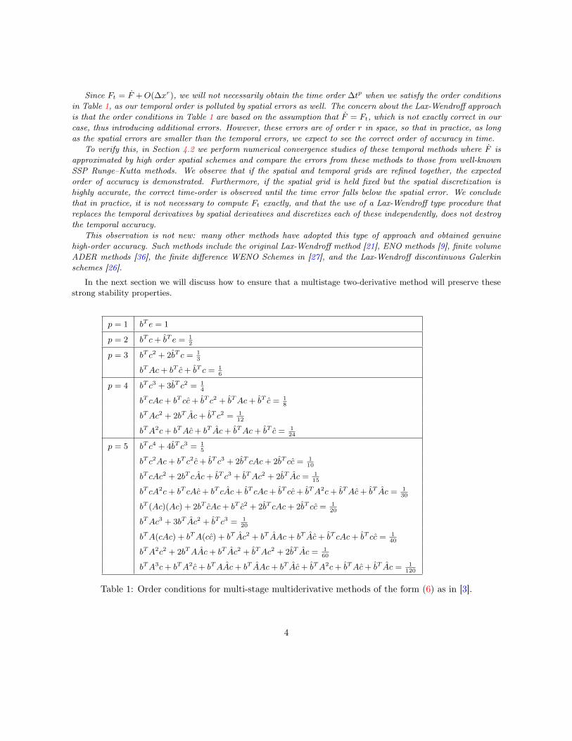
Since Ft = F +O(∆xr), we will not necessarily obtain the time order ∆tp when we satisfy the order conditionsin Table 1, as our temporal order is polluted by spatial errors as well. The concern about the Lax-Wendroff approachis that the order conditions in Table 1 are based on the assumption that F = Ft, which is not exactly correct in ourcase, thus introducing additional errors. However, these errors are of order r in space, so that in practice, as longas the spatial errors are smaller than the temporal errors, we expect to see the correct order of accuracy in time.
To verify this, in Section 4.2 we perform numerical convergence studies of these temporal methods where F isapproximated by high order spatial schemes and compare the errors from these methods to those from well-knownSSP Runge–Kutta methods. We observe that if the spatial and temporal grids are refined together, the expectedorder of accuracy is demonstrated. Furthermore, if the spatial grid is held fixed but the spatial discretization ishighly accurate, the correct time-order is observed until the time error falls below the spatial error. We concludethat in practice, it is not necessary to compute Ft exactly, and that the use of a Lax-Wendroff type procedure thatreplaces the temporal derivatives by spatial derivatives and discretizes each of these independently, does not destroythe temporal accuracy.
This observation is not new: many other methods have adopted this type of approach and obtained genuinehigh-order accuracy. Such methods include the original Lax-Wendroff method [21], ENO methods [9], finite volumeADER methods [36], the finite difference WENO Schemes in [27], and the Lax-Wendroff discontinuous Galerkinschemes [26].
In the next section we will discuss how to ensure that a multistage two-derivative method will preserve thesestrong stability properties.
p = 1 bT e = 1
p = 2 bT c+ bT e = 12
p = 3 bT c2 + 2bT c = 13
bTAc+ bT c+ bT c = 16
p = 4 bT c3 + 3bT c2 = 14
bT cAc+ bT cc+ bT c2 + bTAc+ bT c = 18
bTAc2 + 2bT Ac+ bT c2 = 112
bTA2c+ bTAc+ bT Ac+ bTAc+ bT c = 124
p = 5 bT c4 + 4bT c3 = 15
bT c2Ac+ bT c2c+ bT c3 + 2bT cAc+ 2bT cc = 110
bT cAc2 + 2bT cAc+ bT c3 + bTAc2 + 2bT Ac = 115
bT cA2c+ bT cAc+ bT cAc+ bT cAc+ bT cc+ bTA2c+ bTAc+ bT Ac = 130
bT (Ac)(Ac) + 2bT cAc+ bT c2 + 2bT cAc+ 2bT cc = 120
bTAc3 + 3bT Ac2 + bT c3 = 120
bTA(cAc) + bTA(cc) + bT Ac2 + bT AAc+ bT Ac+ bT cAc+ bT cc = 140
bTA2c2 + 2bTAAc+ bT Ac2 + bTAc2 + 2bT Ac = 160
bTA3c+ bTA2c+ bTAAc+ bT AAc+ bT Ac+ bTA2c+ bTAc+ bT Ac = 1120
Table 1: Order conditions for multi-stage multiderivative methods of the form (6) as in [3].
4
2 The SSP condition for multiderivative methods
2.1 Motivating ExamplesTo understand the strong stability condition for multiderivative methods, we consider the strong stability propertiesof a multiderivative building block of the form
un+1 = un + α∆tF (un) + β∆t2F (un),
and begin with the simple linear one-way wave equation Ut = Ux. This equation has the property that its secondderivative in time is, with the assumption of sufficient smoothness, also the second derivative in space:
Utt = (Ux)t = (Ut)x = Uxx.
We will use this convenient fact in a Lax-Wendroff type approach to define F (un) by a spatial discretization ofUxx.
For this problem, we define F by the original first-order upwind method
F (un)j :=1
∆x
(unj+1 − unj
)≈ Ux(xj), (7a)
and F by the second order centered discretization to Uxx:
F (un)j :=1
∆x2
(unj+1 − 2unj + unj−1
)≈ Uxx(xj). (7b)
These spatial discretizations are total variation diminishing (TVD) in the following sense:
un+1 = un + ∆tF (un) is TVD for ∆t ≤ ∆x, (8a)
un+1 = un + ∆t2F (un) is TVD for ∆t ≤√
2
2∆x. (8b)
Remark 2. Note that we chose a second derivative F in space that is not an exact derivative Ft(un) of F (un) inthe method-of-lines formulation. However, as noted in Remark 1 and will be shown in the convergence studies, if thespatial and temporal grids are co-refined, this provides a sufficiently accurate approximation to F (un). The exactderivative can be obtained by applying the upwind differentiation operator to the solution twice, which produces
Ft :=1
∆x2
(unj+2 − 2unj+1 + unj
).
However, computing F = Ft using this formulation does not satisfy the condition (8b) for any value of ∆t.
To establish the TVD properties of the multiderivative building block we decompose it:
un+1 = un + α∆tF (un) + β∆t2F (un) = aun + α∆tF (un) + (1− a)un + β∆t2F (un)
= a(un +
α
a∆tF (un)
)+ (1− a)
(un +
β
1− a∆t2F (un)
).
It follows that for any 0 ≤ a ≤ 1 this is a convex combination of terms of the form (8a) and (8b), and so
‖un+1‖TV ≤ a∥∥∥(un +
α
a∆tF (un)
)∥∥∥TV
+ (1− a)
∥∥∥∥(un +β
1− a∆t2F (un)
)∥∥∥∥TV
≤ a ‖un‖TV + (1− a) ‖un‖TV ≤ ‖un‖TV
5
for time-steps satisfying ∆t ≤ aα
∆x and ∆t2 ≤ 1−a2β
∆x2. The first restriction relaxes as a increases while the secondbecomes tighter as a increases, so that the value of a that maximizes these conditions occurs when these are equal.This is given by
a2 +α2
2βa− α2
2β= 0, =⇒ a =
α√α2 + 8β − α2
4β.
Using this SSP analysis, we conclude that∥∥∥un + α∆tF (un) + β∆t2F (un)∥∥∥TV≤ ‖un‖TV for ∆t ≤
√α2 + 8β − α
4β∆x. (9)
Of course, for this simple example we can directly compute the value of ∆t for which the multiderivative buildingblock is TVD. That is, with λ := ∆t
∆x≥ 0, we observe that
‖un+1‖TV =∥∥((1− αλ− 2βλ2)unj + (αλ+ βλ2)unj+1 + βλ2unj−1
)∥∥TV≤ ‖un‖TV ,
provided that
1− αλ− 2βλ2 ≥ 0 ⇐⇒ λ ≤√α2 + 8β − α
4β.
We see that for this case, the SSP bound is sharp: the convex combination approach provides us exactly the samebound as directly computing the requirements for total variation.
We wish to generalize this for cases in which the second derivative condition (8b) holds for ∆t ≤ K∆tFE whereK can take on any positive value, not just
√2
2. For the two-derivative building block method this can be done
quite easily:
Theorem 1. Given F and F such that
‖un + ∆tF (un)‖ ≤ ‖un‖ for ∆t ≤ ∆tFE,
and‖un + ∆t2F (un)‖ ≤ ‖un‖ for ∆t ≤ K∆tFE,
the two-derivative building blockun+1 = un + α∆tF (un) + β∆t2F (un)
satisfies the monotonicity condition ‖un+1‖ ≤ ‖un‖ under the time-step restriction
∆t ≤ K
2β
(√α2K2 + 4β − αK
)∆tFE.
Proof. As above, we rewrite
un+1 = a(un +
α
a∆tF (un)
)+ (1− a)
(un +
β
1− a∆t2F (un)
),
which is a convex combination provided that 0 ≤ a ≤ 1. The time-step restriction that follows from this convexcombination must satisfy α
a∆t ≤ ∆tFE and β
1−a∆t2 ≤ K2∆t2FE. The first condition becomes ∆t ≤ aα
∆tFE while
the second is ∆t ≤√
1−aβK∆tFE. We observe that on 0 ≤ a ≤ 1 the first term encourages a larger a while the
second term is less restrictive with a smaller a. The two conditions are balanced, and thus the allowable time-stepis maximized, when we equate the right hand sides:
a
α=
√1− aβ
K → a =αK
2β
(√α2K2 + 4β − αK
).
Now using the first condition, ∆t ≤ aα
∆tFE we obtain our result.
6
A more realistic motivating example is the unique two-stage fourth order method
u∗ = un +∆t
2F (un) +
∆t2
8F (un),
un+1 = un + ∆tF (un) +∆t2
6(F (un) + 2F (u∗)). (10)
The first stage of the method is a Taylor series method with ∆t2, while the second stage can be written
un+1 = un + ∆tF (un) +∆t2
6(F (un) + 2F (u∗))
= a
(u∗ − ∆t
2F (un)− ∆t2
8F (un)
)+ (1− a)un + ∆tF (un) +
∆t2
6(F (un) + 2F (u∗))
= (1− a)
(un +
1− a2
1− a∆tF (un) +16− a
8
1− a ∆t2F (un)
)+ a
(u∗ +
∆t2
3aF (u∗)
).
For 0 ≤ a ≤ 1 this is a convex combination of two terms. The first term is of the form (9), which gives the time-steprestriction
∆t ≤ 6
4− 3a
(√(5
4a2 − 10
3a+
7
3
)− 1 +
a
2
)∆tFE.
The second is of the form (8b), so we have ∆t ≤√
3a2
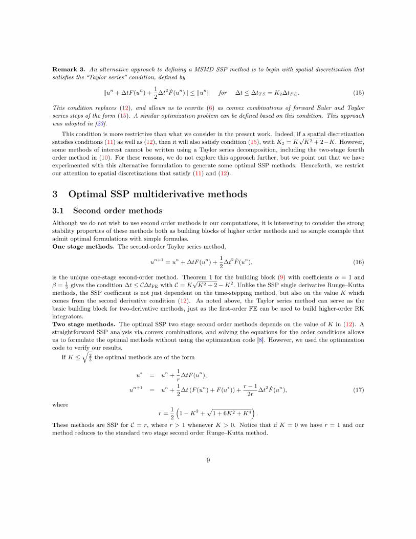
∆tFE. We plot these two in Figure 1, and we observe that thefirst term is decreasing in a (blue line) while the second term is increasing in a (red line). As a result, we obtain theoptimal allowable time-step by setting these two equal, which yields a ≈ 0.3072182638002141 and the correspondingSSP coefficient, C ≈ 0.6788426884782078. A direct computation of the TVD time-step for this case, which takesadvantage of the linearity of the problem and the spatial discretization, gives the bound ∆t ≤ (
√3− 1) > 0.6788.
This shows that, as we expect, the SSP condition is not always sharp.The convex combination approach becomes more complicated when dealing with multi-stage methods. It is the
most appropriate approach for developing an understanding of the strong stability property of a given method.However, it is not computationally efficient for finding optimal SSP methods. In the following section, we showhow to generalize the convex combination decomposition approach and we use this generalization to formulate anSSP optimization problem along the lines of [16, 19].
2.2 Formulating the SSP optimization problemAs above, we begin with the hyperbolic conservation law (1) and adopt a spatial discretization so that we have thesystem of ODEs (2). The spatial discretization F is specially designed so that it satisfies the forward Euler (firstderivative) condition
Forward Euler condition ‖un + ∆tF (un)‖ ≤ ‖un‖ for ∆t ≤ ∆tFE , (11)
for the desired stability property indicated by the convex functional ‖ · ‖. For multiderivative methods, in additionto the first derivative, we need to appropriately approximate the second derivative in time utt, to which we representthe discretization as F . It is not immediately obvious what should be the form of a condition that would accountfor the effect of the ∆t2F term. Motivated by the examples in the previous sections, we choose the
Second derivative condition ‖un + ∆t2F (un)‖ ≤ ‖un‖ for ∆t ≤ K∆tFE , (12)
whereK is a scaling factor that compares the stability condition of the second derivative term to that of the forwardEuler term. Given conditions (11) and (12), we wish to formulate sufficient conditions so that the multiderivative
7
method (6) satisfies the desired monotonicity condition under a given time-step. First, we write the method (6) inan equivalent matrix-vector form
y = eun + ∆tSF (y) + ∆t2SF (y), (13)
where
S =
[A 0bT 0
]and S =
[A 0bT 0
]and e is a vector of ones. We are now ready to state our result:
Theorem 2. Given spatial discretizations F and F that satisfy (11) and (12), a two-derivative multistage methodof the form (13) preserves the strong stability property ‖un+1‖ ≤ ‖un‖ under the time-step restriction ∆t ≤ r∆tFE
if satisfies the conditions (I + rS +
r2
K2S
)−1
e ≥ 0 (14a)
r
(I + rS +
r2
K2S
)−1
S ≥ 0 (14b)
r2
K2
(I + rS +
r2
K2S
)−1
S ≥ 0 (14c)
for some r > 0. In the above conditions, the inequalities are understood component-wise.
Proof. We begin with the method (13), and add the terms rSy and rSy to both sides to obtain(I + rS + rS
)y = une + rS
(y +
∆t
rF (y)
)+ rS
(y +
∆t2
rF (y)
),
y = R(eun) + P
(y +
∆t
rF (y)
)+Q
(y +
∆t2
rF (y)
),
whereR =
(I + rS + rS
)−1
, P = rRS, Q = rRS.
If the elements of P , Q, and Re are all non-negative, and if R + P + Q = I, then these three terms describe aconvex combination of terms which are SSP, and the resulting value is SSP as well
‖y‖ ≤ R‖eun‖+ P‖y +∆t
rF (y)‖+Q‖y +
∆t2
rF (y)‖,
under the time-step restrictions ∆t ≤ r∆tFE and ∆t ≤ K√r∆tFE. As we observed above, the optimal time-step
is given when these two are set equal, so we require r = K√r. Conditions (14a)–(14c) now ensure that P ≥ 0,
Q ≥ 0, and Re ≥ 0 component-wise for r = r2
K2 , and our method (13) preserves the strong stability condition‖un+1‖ ≤ ‖un‖ under the time-step restriction ∆t ≤ r∆tFE .
This theorem gives us the conditions for the method (13) to be SSP for any the time-step ∆t ≤ r∆tFE. Thisallows us to formulate the search for optimal SSP two-derivative methods as an optimization problem, similarto [16, 18, 7], where the aim is to find C = max r such that the relevant order conditions (from Section 1.2)and SSP conditions (14a)-(14b) are all satisfied. Based on this, we wrote a Matlab optimization code for findingoptimal two-derivative multistage methods [8], formulated along the lines of David Ketcheson’s code [19] for findingoptimal SSP multistage multistep methods in [17, 2]. We used this to find optimal SSP multistage two-derivativemethods of order up to p = 5. However, we also used our observations on the resulting methods to formulate closedform representations of the optimal SSP multistage two-derivative methods. We present both the numerical andclosed-form optimal methods in the following section.
8
Remark 3. An alternative approach to defining a MSMD SSP method is to begin with spatial discretization thatsatisfies the “Taylor series” condition, defined by
‖un + ∆tF (un) +1
2∆t2F (un)‖ ≤ ‖un‖ for ∆t ≤ ∆tTS = K2∆tFE . (15)
This condition replaces (12), and allows us to rewrite (6) as convex combinations of forward Euler and Taylorseries steps of the form (15). A similar optimization problem can be defined based on this condition. This approachwas adopted in [23].
This condition is more restrictive than what we consider in the present work. Indeed, if a spatial discretizationsatisfies conditions (11) as well as (12), then it will also satisfy condition (15), with K2 = K
√K2 + 2−K. However,
some methods of interest cannot be written using a Taylor series decomposition, including the two-stage fourthorder method in (10). For these reasons, we do not explore this approach further, but we point out that we haveexperimented with this alternative formulation to generate some optimal SSP methods. Henceforth, we restrictour attention to spatial discretizations that satisfy (11) and (12).
3 Optimal SSP multiderivative methods
3.1 Second order methodsAlthough we do not wish to use second order methods in our computations, it is interesting to consider the strongstability properties of these methods both as building blocks of higher order methods and as simple example thatadmit optimal formulations with simple formulas.One stage methods. The second-order Taylor series method,
un+1 = un + ∆tF (un) +1
2∆t2F (un), (16)
is the unique one-stage second-order method. Theorem 1 for the building block (9) with coefficients α = 1 andβ = 1
2gives the condition ∆t ≤ C∆tFE with C = K
√K2 + 2−K2. Unlike the SSP single derivative Runge–Kutta
methods, the SSP coefficient is not just dependent on the time-stepping method, but also on the value K whichcomes from the second derivative condition (12). As noted above, the Taylor series method can serve as thebasic building block for two-derivative methods, just as the first-order FE can be used to build higher-order RKintegrators.Two stage methods. The optimal SSP two stage second order methods depends on the value of K in (12). Astraightforward SSP analysis via convex combinations, and solving the equations for the order conditions allowsus to formulate the optimal methods without using the optimization code [8]. However, we used the optimizationcode to verify our results.
If K ≤√
23the optimal methods are of the form
u∗ = un +1
r∆tF (un),
un+1 = un +1
2∆t (F (un) + F (u∗)) +
r − 1
2r∆t2F (un), (17)
wherer =
1
2
(1−K2 +
√1 + 6K2 +K4
).
These methods are SSP for C = r, where r > 1 whenever K > 0. Notice that if K = 0 we have r = 1 and ourmethod reduces to the standard two stage second order Runge–Kutta method.
9
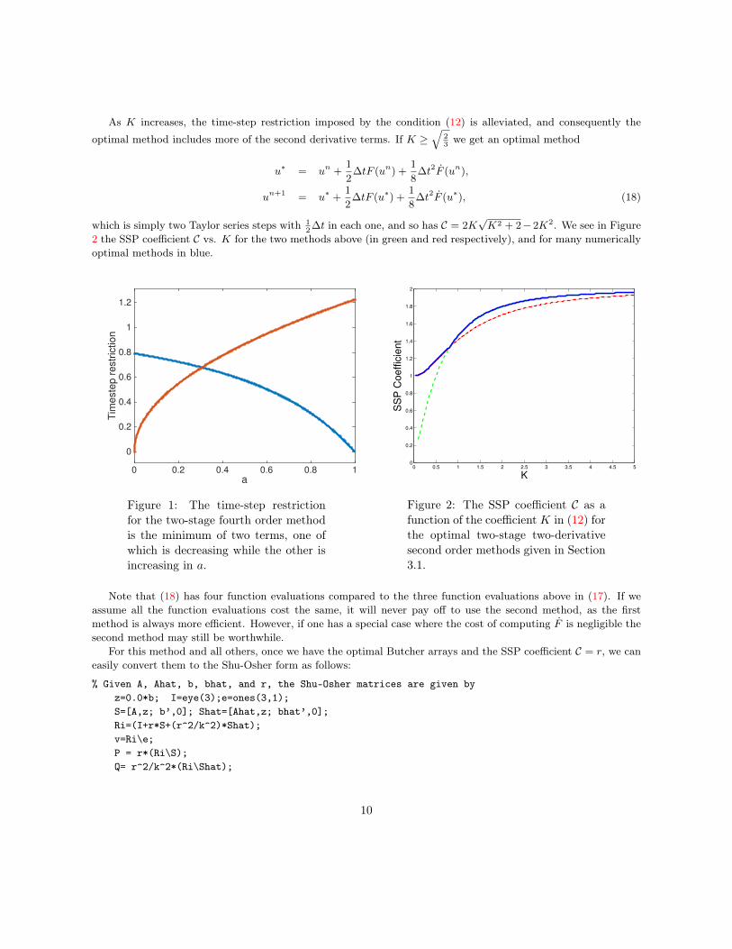
As K increases, the time-step restriction imposed by the condition (12) is alleviated, and consequently the
optimal method includes more of the second derivative terms. If K ≥√
23we get an optimal method
u∗ = un +1
2∆tF (un) +
1
8∆t2F (un),
un+1 = u∗ +1
2∆tF (u∗) +
1
8∆t2F (u∗), (18)
which is simply two Taylor series steps with 12∆t in each one, and so has C = 2K
√K2 + 2−2K2. We see in Figure
2 the SSP coefficient C vs. K for the two methods above (in green and red respectively), and for many numericallyoptimal methods in blue.
a0 0.2 0.4 0.6 0.8 1
Tim
este
p r
estr
iction
0
0.2
0.4
0.6
0.8
1
1.2
Figure 1: The time-step restrictionfor the two-stage fourth order methodis the minimum of two terms, one ofwhich is decreasing while the other isincreasing in a.
0 0.5 1 1.5 2 2.5 3 3.5 4 4.5 50
0.2
0.4
0.6
0.8
1
1.2
1.4
1.6
1.8
2
K
SS
P C
oeffic
ient
Figure 2: The SSP coefficient C as afunction of the coefficient K in (12) forthe optimal two-stage two-derivativesecond order methods given in Section3.1.
Note that (18) has four function evaluations compared to the three function evaluations above in (17). If weassume all the function evaluations cost the same, it will never pay off to use the second method, as the firstmethod is always more efficient. However, if one has a special case where the cost of computing F is negligible thesecond method may still be worthwhile.
For this method and all others, once we have the optimal Butcher arrays and the SSP coefficient C = r, we caneasily convert them to the Shu-Osher form as follows:
% Given A, Ahat, b, bhat, and r, the Shu-Osher matrices are given byz=0.0*b; I=eye(3);e=ones(3,1);S=[A,z; b’,0]; Shat=[Ahat,z; bhat’,0];Ri=(I+r*S+(r^2/k^2)*Shat);v=Ri\e;P = r*(Ri\S);Q= r^2/k^2*(Ri\Shat);
10
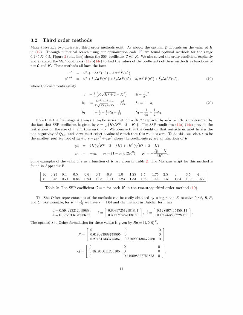
3.2 Third order methodsMany two-stage two-derivative third order methods exist. As above, the optimal C depends on the value of Kin (12). Through numerical search using our optimization code [8], we found optimal methods for the range0.1 ≤ K ≤ 5. Figure 3 (blue line) shows the SSP coefficient C vs. K. We also solved the order conditions explicitlyand analyzed the SSP conditions (14a)-(14c) to find the values of the coefficients of these methods as functions ofr = C and K. These methods all have the form
u∗ = un + a∆tF (un) + a∆t2F (un),
un+1 = un + b1∆tF (un) + b2∆tF (u∗) + b1∆t2F (un) + b2∆t2F (u∗), (19)
where the coefficients satisfy
a = 1r
(K√K2 + 2−K2
)a =
1
2a2
b2 =2K2(1− 1
r)+r
K√K2+2+K2
− r2
3K2 b1 = 1− b2 (20)
b1 = 12− 1
2ab2 − 1
6ab2 =
1
6a− 1
2ab2
Note that the first stage is always a Taylor series method with ∆t replaced by a∆t, which is underscored bythe fact that SSP coefficient is given by r = 1
a
(K√K2 + 2−K2
). The SSP conditions (14a)-(14c) provide the
restrictions on the size of r, and thus on C = r. We observe that the condition that restricts us most here is thenon-negativity of Q3,1, and so we must select a value of r such that this value is zero. To do this, we select r to bethe smallest positive root of p0 + p1r + p2r
2 + p3r3 where the coefficients pi are all functions of K
p0 = 2K(√K2 + 2− 3K) + 4K3(
√K2 + 2−K)
p1 = −a0, p2 = (1− a0)/(2K2), p3 = −a02K
+K
6K3.
Some examples of the value of r as a function of K are given in Table 2. The Matlab script for this method isfound in Appendix B.
K 0.25 0.4 0.5 0.6 0.7 0.8 1.0 1.25 1.5 1.75 2.5 3 3.5 4r 0.48 0.71 0.84 0.94 1.03 1.11 1.23 1.33 1.39 1.44 1.51 1.54 1.55 1.56
Table 2: The SSP coefficient C = r for each K in the two-stage third order method (19).
The Shu-Osher representations of the methods can be easily obtained by using r and K to solve for r, R,P ,and Q. For example, for K = 1√
2we have r = 1.04 and the method in Butcher form has
a = 0.594223212099088,
a = 0.176550612898679,b =
[0.693972512991841
0.306027487008159
], b =
[0.128597465450411
0.189553898228989
].
The optimal Shu Osher formulation for these values is given by Re = (1, 0, 0)T ,
P =
0 0 0
0.618033988749895 0 0
0.271611333775367 0.318290138472780 0
Q =
0 0 0
0.381966011250105 0 0
0 0.410098527751853 0
.
11
0 1 2 3 4 50
0.2
0.4
0.6
0.8
1
1.2
1.4
1.6
K
SS
P C
oeffic
ient
Figure 3: The SSP coefficient vs. K fortwo stage methods. Third order methodsare in blue, the fourth order methods arered.
0 0.5 1 1.5 2 2.50
0.5
1
1.5
2
K
SS
P C
oeffic
ient
Figure 4: The SSP coefficient vs. K forthree stage methods. Fourth order meth-ods are in blue (top line), the fifth ordermethods in red (bottom line).
3.3 Fourth order methods3.3.1 Fourth order methods: The two-stage fourth-order method
The two-stage two-derivative fourth order method (10) is unique; there is only one set of coefficients that satisfythe fourth order conditions for this number of stages and derivatives. The method is
u∗ = un +∆t
2F (un) +
∆t2
8F (un)
un+1 = un + ∆tF (un) +∆t2
6(F (un) + 2F (u∗)).
The first stage of the method is a Taylor series method with ∆t2, while the second stage can be written as a linear
combination of a forward Euler and a second-derivative term (but not a Taylor series term). The SSP coefficientof this method is larger as K increases, as can be seen in Figure 3.
To ensure that the SSP conditions (14a)-(14c) are satisfied, we need to select the largest r so that all the termsare non-negative. We observed from numerical optimization that in the case of the two-stage fourth order methodthe term (Re)3 gives the most restrictive condition: if we choose r to ensure that this term is non-negative, all theother conditions are satisfied. Satisfying this condition, the SSP coefficient C = r is given by the smallest positiveroot of the polynomial:
(Re)3 = r4 + 4K2r3 − 12K2r2 − 24K4r + 24K4.
The Shu-Osher decomposition for the optimal method corresponding to this value of K is
u∗ =
(1− 4rK2 + r2
8K2
)un +
r
2
(un +
∆t
rF (un)
)+
r2
8K2
(un +
K2
r2∆t2F (un)
)(21)
un+1 = r
(1− r2
6K2
)(un +
∆t
rF (un)
)+r2(4K2 − r2)
24K4
(un +
K2
r2∆t2F (un)
)+
r2
3K2
(u∗ +
K2
r2∆t2F (u∗)
).
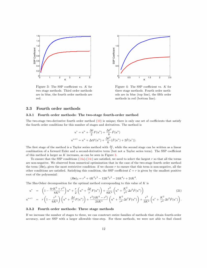
3.3.2 Fourth order methods: Three stage methods
If we increase the number of stages to three, we can construct entire families of methods that obtain fourth-orderaccuracy, and are SSP with a larger allowable time-step. For these methods, we were not able to find closed
12
form solutions, but our optimization code [8] produced methods for various values of K. The SSP coefficient asa function of K for these methods is given in Figure 3, and we give the coefficients for selected methods in bothButcher array and Shu-Osher form in Appendix A.
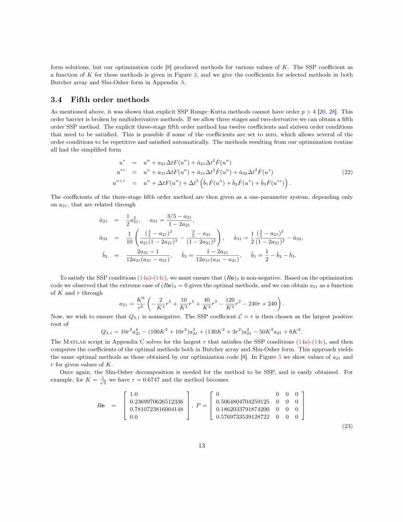
3.4 Fifth order methodsAs mentioned above, it was shown that explicit SSP Runge–Kutta methods cannot have order p > 4 [20, 28]. Thisorder barrier is broken by multiderivative methods. If we allow three stages and two-derivative we can obtain a fifthorder SSP method. The explicit three-stage fifth order method has twelve coefficients and sixteen order conditionsthat need to be satisfied. This is possible if some of the coefficients are set to zero, which allows several of theorder conditions to be repetitive and satisfied automatically. The methods resulting from our optimization routineall had the simplified form
u∗ = un + a21∆tF (un) + a21∆t2F (un)
u∗∗ = un + a31∆tF (un) + a31∆t2F (un) + a32∆t2F (u∗) (22)
un+1 = un + ∆tF (un) + ∆t2(b1F (un) + b2F (u∗) + b3F (u∗∗)
).
The coefficients of the three-stage fifth order method are then given as a one-parameter system, depending onlyon a21, that are related through
a21 =1
2a2
21, a31 =3/5− a21
1− 2a21,
a32 =1
10
(( 3
5− a21)2
a21(1− 2a21)3−
35− a21
(1− 2a21)2
), a31 =
1
2
( 35− a21)2
(1− 2a21)2− a32,
b2 =2a31 − 1
12a21(a31 − a21), b3 =
1− 2a21
12a31(a31 − a21), b1 =
1
2− b2 − b3.
To satisfy the SSP conditions (14a)-(14c), we must ensure that (Re)3 is non-negative. Based on the optimizationcode we observed that the extreme case of (Re)3 = 0 gives the optimal methods, and we can obtain a21 as a functionof K and r through
a21 =K6
r6
(− 2
K4r5 +
10
K4r4 +
40
K2r3 − 120
K2r2 − 240r + 240
).
Now, we wish to ensure that Q3,1 is nonnegative. The SSP coefficient C = r is then chosen as the largest positiveroot of
Q3,1 = 10r2a421 − (100K2 + 10r2)a3
21 + (130K2 + 3r2)a221 − 50K2a21 + 6K2.
The Matlab script in Appendix C solves for the largest r that satisfies the SSP conditions (14a)-(14c), and thencomputes the coefficients of the optimal methods both in Butcher array and Shu-Osher form. This approach yieldsthe same optimal methods as those obtained by our optimization code [8]. In Figure 5 we show values of a21 andr for given values of K.
Once again, the Shu-Osher decomposition is needed for the method to be SSP, and is easily obtained. Forexample, for K = 1√
2we have r = 0.6747 and the method becomes
Re =
1.0
0.2369970626512336
0.7810723816004148
0.0
, P =
0 0 0 0
0.5064804704259125 0 0 0
0.1862033791874200 0 0 0
0.5769733539128722 0 0 0
(23)
13
0 0.5 1 1.5 2 2.50
0.2
0.4
0.6
0.8
1
K
SS
P C
oe
ffic
ien
t
K a21 C K a21 C0.1 0.7947 0.1452 1.1 0.7393 0.81140.2 0.7842 0.2722 1.2 0.7374 0.83350.3 0.7751 0.3814 1.3 0.7359 0.85230.4 0.7674 0.4741 1.4 0.7346 0.86830.5 0.7609 0.5520 1.5 0.7334 0.88190.6 0.7555 0.6171 1.6 0.7324 0.89370.7 0.7510 0.6712 1.7 0.7316 0.90390.8 0.7472 0.7162 1.8 0.7309 0.91270.9 0.7441 0.7537 1.9 0.7302 0.92051.0 0.7415 0.7851 2.0 0.7296 0.9273
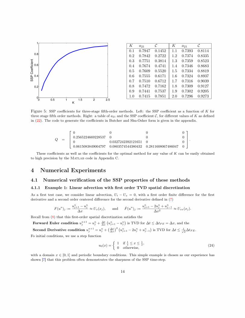
Figure 5: SSP coefficients for three-stage fifth-order methods. Left: the SSP coefficient as a function of K forthree stage fifth order methods. Right: a table of a21 and the SSP coefficient C, for different values of K as definedin (22). The code to generate the coefficients in Butcher and Shu-Osher form is given in the appendix.
Q =
0 0 0 0
0.2565224669228537 0 0 0
0 0.0327242392121651 0 0
0.0615083849004797 0.0803574544380432 0.2811608067486047 0
.These coefficients as well as the coefficients for the optimal method for any value of K can be easily obtained
to high precision by the Matlab code in Appendix C.
4 Numerical Experiments
4.1 Numerical verification of the SSP properties of these methods4.1.1 Example 1: Linear advection with first order TVD spatial discretization
As a first test case, we consider linear advection, Ut − Ux = 0, with a first order finite difference for the firstderivative and a second order centered difference for the second derivative defined in (7)
F (un)j :=unj+1 − unj
∆x≈ Ux(xj), and F (un)j :=
unj+1 − 2unj + unj−1
∆x2≈ Uxx(xj).
Recall from (8) that this first-order spatial discretization satisfies the
Forward Euler condition un+1j = unj + ∆t
∆x
(unj+1 − unj
)is TVD for ∆t ≤ ∆tFE = ∆x, and the
Second Derivative condition un+1j = unj +
(∆t∆x
)2 (unj+1 − 2unj + unj−1
)is TVD for ∆t ≤ 1√
2∆tFE .
Fo initial conditions, we use a step function
u0(x) =
{1 if 1
4≤ x ≤ 1
2,
0 otherwise,(24)
with a domain x ∈ [0, 1] and periodic boundary conditions. This simple example is chosen as our experience hasshown [7] that this problem often demonstrates the sharpness of the SSP time-step.
14
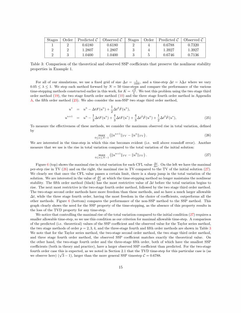
Stages Order Predicted C Observed C Stages Order Predicted C Observed C1 2 0.6180 0.6180 2 4 0.6788 0.73202 2 1.2807 1.2807 3 4 1.3927 1.39272 3 1.0400 1.0400 3 5 0.6746 0.7136
Table 3: Comparison of the theoretical and observed SSP coefficients that preserve the nonlinear stabilityproperties in Example 1.
For all of our simulations, we use a fixed grid of size ∆x = 11600
, and a time-step ∆t = λ∆x where we vary0.05 ≤ λ ≤ 1. We step each method forward by N = 50 time-steps and compare the performance of the varioustime-stepping methods constructed earlier in this work, for K =
√2
2. We test this problem using the two stage third
order method (19), the two stage fourth order method (10) and the three stage fourth order method in AppendixA, the fifth order method (23). We also consider the non-SSP two stage third order method,
u∗ = un −∆tF (un) +1
2∆t2F (un),
un+1 = un − 1
3∆tF (un) +
4
3∆tF (u∗) +
4
3∆t2F (un) +
1
2∆t2F (u∗), (25)
To measure the effectiveness of these methods, we consider the maximum observed rise in total variation, definedby
max0≤n≤N−1
(‖un+1‖TV − ‖un‖TV
). (26)
We are interested in the time-step in which this rise becomes evident (i.e. well above roundoff error). Anothermeasure that we use is the rise in total variation compared to the total variation of the initial solution:
max0≤n≤N−1
(‖un+1‖TV − ‖u0‖TV
). (27)
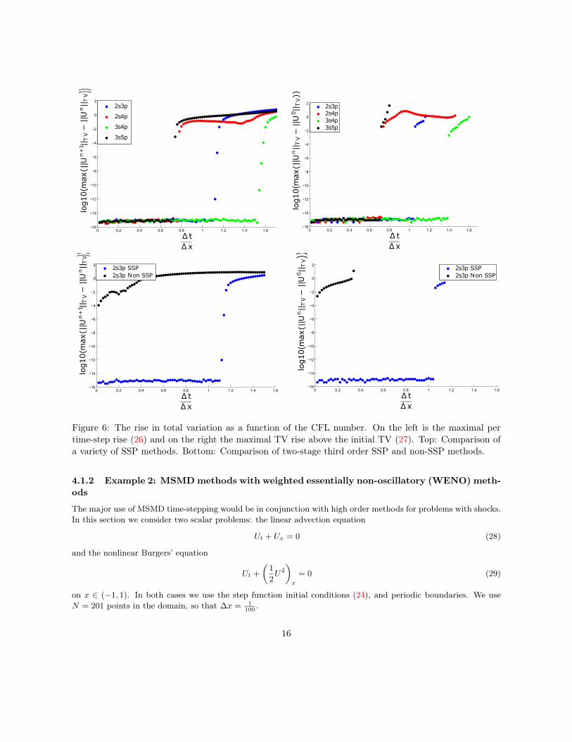
Figure 6 (top) shows the maximal rise in total variation for each CFL value ∆t∆x
. On the left we have the maximalper-step rise in TV (26) and on the right, the maximal rise in TV compared to the TV of the initial solution (27).We clearly see that once the CFL value passes a certain limit, there is a sharp jump in the total variation of thesolution. We are interested in the value of ∆t
∆xat which the time-stepping method no longer maintains the nonlinear
stability. The fifth order method (black) has the most restrictive value of ∆t before the total variation begins torise. The next most restrictive is the two-stage fourth order method, followed by the two stage third order method.The two-stage second order methods have more freedom than these methods, and so have a much larger allowable∆t, while the three stage fourth order, having the most freedom in the choice of coefficients, outperforms all theother methods. Figure 6 (bottom) compares the performance of the non-SSP method to the SSP method. Thisgraph clearly shows the need for the SSP property of the time-stepping, as the absence of this property results inthe loss of the TVD property for any time-step.
We notice that controlling the maximal rise of the total variation compared to the initial condition (27) requires asmaller allowable time-step, so we use this condition as our criterion for maximal allowable time-step. A comparisonof the predicted (i.e. theoretical) values of the SSP coefficient and the observed value for the Taylor series method,the two stage methods of order p = 2, 3, 4, and the three-stage fourth and fifth order methods are shown in Table 3We note that for the Taylor series method, the two-stage second order method, the two stage third order method,and three stage fourth order method, the observed SSP coefficient matches exactly the theoretical value. Onthe other hand, the two-stage fourth order and the three-stage fifth order, both of which have the smallest SSPcoefficients (both in theory and practice), have a larger observed SSP coefficient than predicted. For the two-stagefourth order case this is expected, as we noted in Section 2.1 that the TVD time-step for this particular case is (aswe observe here) (
√3− 1), larger than the more general SSP timestep C = 0.6788.
15
� ��� ��� ��� ��� � ��� ��� ������
���
���
���
��
��
��
��
�
�
���������������� �� �� ������ ������
� �
�
����
����
����
����
0 0.2 0.4 0.6 0.8 1 1.2 1.4 1.6−16
−14
−12
−10
−8
−6
−4
−2
0
2
log10(m
ax(|
|Un||
TV
−||U
0||
TV))
∆ t
∆x
2s3p
2s4p
3s4p
3s5p
0 0.2 0.4 0.6 0.8 1 1.2 1.4 1.6−16
−14
−12
−10
−8
−6
−4
−2
0
2
log10(m
ax(|
|Un
+1 || T
V−
||U
n||
TV ))
∆ t
∆x
2s3p SSP
2s3p Non SSP
0 0.2 0.4 0.6 0.8 1 1.2 1.4 1.6−16
−14
−12
−10
−8
−6
−4
−2
0
2
log10(m
ax(|
|Un||
TV
−||U
0||
TV))
∆ t
∆x
2s3p SSP
2s3p Non SSP
Figure 6: The rise in total variation as a function of the CFL number. On the left is the maximal pertime-step rise (26) and on the right the maximal TV rise above the initial TV (27). Top: Comparison ofa variety of SSP methods. Bottom: Comparison of two-stage third order SSP and non-SSP methods.
4.1.2 Example 2: MSMDmethods with weighted essentially non-oscillatory (WENO) meth-ods
The major use of MSMD time-stepping would be in conjunction with high order methods for problems with shocks.In this section we consider two scalar problems: the linear advection equation
Ut + Ux = 0 (28)
and the nonlinear Burgers’ equation
Ut +
(1
2U2
)x
= 0 (29)
on x ∈ (−1, 1). In both cases we use the step function initial conditions (24), and periodic boundaries. We useN = 201 points in the domain, so that ∆x = 1
100.
16
0 0.2 0.4 0.6 0.8 1 1.2 1.4 1.6−12
−10
−8
−6
−4
−2
0
lo
g10(
ma
x (|
|Un||
TV
−||U
0||
TV
))
∆ t
∆x
2s3p
2s4p
3s4p
3s5p
0 0.2 0.4 0.6 0.8 1 1.2 1.4 1.6−16
−14
−12
−10
−8
−6
−4
−2
0
2
log10(m
ax(|
|Un||
TV
−||U
0||
TV))
∆ t
∆x
2s3p
2s4p
3s4p
3s5p
0 0.2 0.4 0.6 0.8 1 1.2−14
−12
−10
−8
−6
−4
−2
0
2
log10(m
ax(|
|Un||
TV
−||U
0||
TV))
∆ t
∆x
2s3p SSP
2s3p Non SSP
0 0.2 0.4 0.6 0.8 1 1.2 1.4 1.6−16
−14
−12
−10
−8
−6
−4
−2
0
2
log10(m
ax(|
|Un||
TV
−||U
0||
TV))
∆ t
∆x
2s3p SSP
2s3p Non SSP
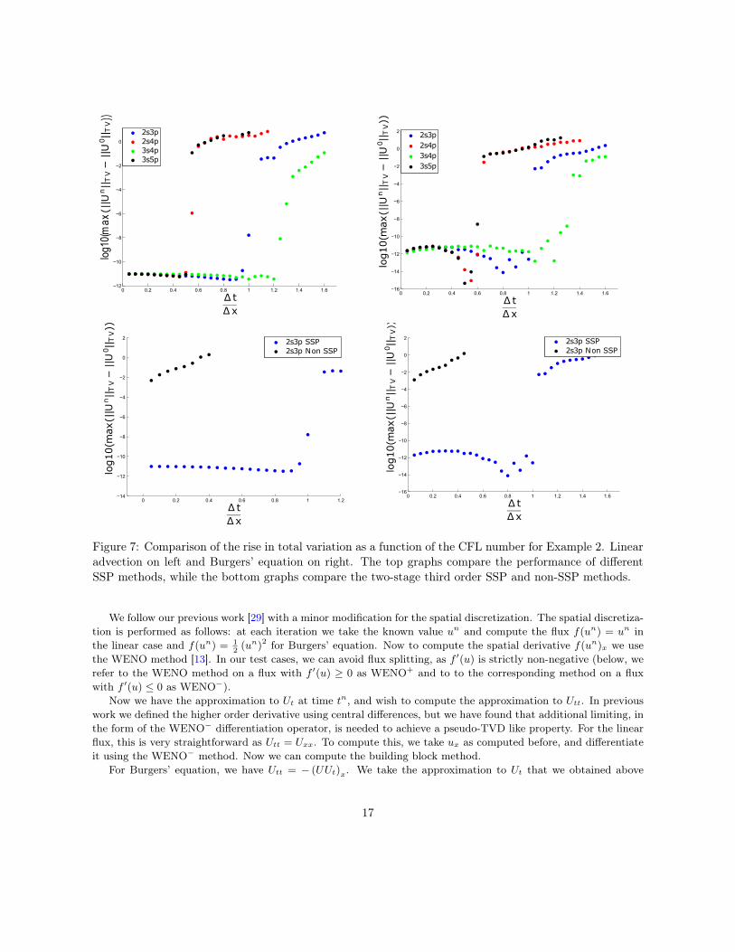
Figure 7: Comparison of the rise in total variation as a function of the CFL number for Example 2. Linearadvection on left and Burgers’ equation on right. The top graphs compare the performance of differentSSP methods, while the bottom graphs compare the two-stage third order SSP and non-SSP methods.
We follow our previous work [29] with a minor modification for the spatial discretization. The spatial discretiza-tion is performed as follows: at each iteration we take the known value un and compute the flux f(un) = un inthe linear case and f(un) = 1
2(un)2 for Burgers’ equation. Now to compute the spatial derivative f(un)x we use
the WENO method [13]. In our test cases, we can avoid flux splitting, as f ′(u) is strictly non-negative (below, werefer to the WENO method on a flux with f ′(u) ≥ 0 as WENO+ and to to the corresponding method on a fluxwith f ′(u) ≤ 0 as WENO−).
Now we have the approximation to Ut at time tn, and wish to compute the approximation to Utt. In previouswork we defined the higher order derivative using central differences, but we have found that additional limiting, inthe form of the WENO− differentiation operator, is needed to achieve a pseudo-TVD like property. For the linearflux, this is very straightforward as Utt = Uxx. To compute this, we take ux as computed before, and differentiateit using the WENO− method. Now we can compute the building block method.
For Burgers’ equation, we have Utt = − (UUt)x. We take the approximation to Ut that we obtained above
17
using WENO+, we multiply it by un and differentiate in space using WENO−. The choice of WENO+ followedby WENO− is made by analogy to the first order finite difference for the linear advection case, where we use adifferentiation operator D+ followed by the downwind differentiation operator D− to produce a centered differencefor the second derivative. The second derivative condition (12) was satisfied by this approach. Now we computethe building block method with the approximations to Ut and Utt. In pseudocode, the building block calculationtakes the form:
f(un) =1
2(un)2; unt = WENO+(f(un));
f ′(un) = un; f(un)t = f ′(un)unt untt = WENO−(f(un)t)
un+1 = un + α∆tunt + β∆t2untt.
We use the two stage third order SSP method (19), and the non-SSP method (25) the two stage fourth order method(10) and the three stage fourth order method in Appendix A, the fifth order method (23). In these simulations,we use ∆t = λ∆x where 0.05 ≤ λ ≤ 1.6, and step up to Tfinal = 1.0. At each time-step we compute (27), themaximal rise in total variation compared to the total variation of the initial solution. In Figure 7 we observe similarbehavior to those of the linear advection with first order time-stepping, and once again see that the SSP methodis needed to preserve the nonlinear stability of WENO as well.
4.2 Convergence studiesAs a final test case, we investigate the accuracy of the proposed schemes in conjunction with various high orderspatial discretization operators. We perform several tests that demonstrate that these methods converge with thecorrect order for linear and nonlinear problems. In the first study (Example 3), we refine the grid only in time, andshow that if the spatial discretization is sufficiently accurate the multi-derivative methods exhibit the design-orderof convergence. We also compare the performance of the third order multi-derivative method to the three stagethird order explicit SSP Runge–Kutta method (SSPRK3,3) [32] and show that the convergence properties are thesame, indicating that the additional error in approximating Ft does not affect the accuracy of the method. In thesecond study (Example 4) we co-refine the spatial and temporal grid by setting ∆t = λ∆x for a fixed λ, and shrink∆x. We observed that since the order of the spatial method is higher than the order of the temporal discretization,the time-stepping method achieves the design-order of accuracy both for linear and nonlinear problems.Example 3a: temporal grid refinement with pseudospectral approximation of the spatial derivative.We begin with a linear advection problem Ut + Ux = 0 with periodic boundary conditions and initial conditionsu0(x) = 0.5 + 0.5 sin(x) on the spatial domain x ∈ [0, 2π]. We discretize the spatial grid with N = 41 equidistantpoints and use the Fourier pseudospectral differentiation matrix D [10] to compute F ≈ −Ux ≈ −Du. We usea Lax-Wendroff approach to approximate Ft ≈ Uxx ≈ D2u. In this case, the solution is a sine wave, so thatthe pseudospectral method is exact. For this reason, the spatial discretization of F is exact and contributes noerrors, and the second derivative Ft is also exact Ft = utt = −Dut = −DF = D2u = F . We use a range of timesteps, ∆t = λ∆x where we pick λ = 0.8, 0.7, 0.6, 0.5, 0.4, 0.3, 0.2, 0.1, and 0.05 to compute the solution to final timeTf = 2.0.
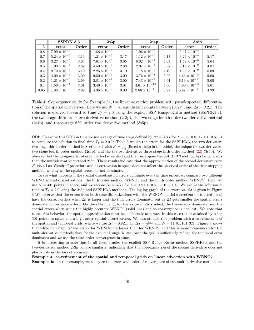
In Table 4 we list the errors for the SSPRK3,3, the two derivative two stage third order method in Section 3.2with K = 1√
2(listed as 2s3p in the table), the unique the two derivative two stage fourth order method (2s4p),
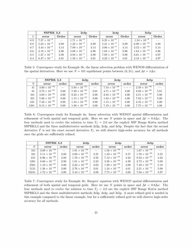
and the the two derivative three stage fifth order method (22) (3s5p). We observe that the design-order of eachmethod is verified. It is interesting to note that the SSPRK3,3 method has larger errors than the multiderivativemethod 2s3p, demonstrating that the additional computation of F does improve the quality of the solution.Example 3b: temporal grid refinement with WENO approximations of the spatial derivative. Usingthe same problem as above we discretize the spatial grid with N = 101 equidistant points and use the ninth orderweighted essentially non-oscillatory method (WENO9) [1] to differentiate the spatial derivatives. It is interestingto note that although the PDE we solve is linear, the use of the nonlinear method WENO9 results in a non-linear
18
SSPRK 3,3 2s3p 2s4p 3s5pλ error Order error Order error Order error Order
0.8 7.99× 10⁻⁵ — 1.86× 10⁻⁵ — 1.96× 10⁻⁶ — 6.47× 10⁻⁸ —0.7 5.24× 10⁻⁵ 3.16 1.21× 10⁻⁵ 3.17 1.12× 10⁻⁶ 4.17 3.24× 10⁻⁸ 5.17
0.6 3.27× 10⁻⁵ 3.04 7.61× 10⁻⁶ 3.05 6.02× 10⁻⁷ 4.04 1.49× 10⁻⁸ 5.04
0.5 1.93× 10⁻⁵ 2.87 4.50× 10⁻⁶ 2.88 2.97× 10⁻⁷ 3.87 6.12× 10⁻⁹ 4.87
0.4 9.70× 10⁻⁶ 3.10 2.25× 10⁻⁶ 3.10 1.18× 10⁻⁷ 4.10 1.96× 10⁻⁹ 5.09
0.3 4.09× 10⁻⁶ 3.00 9.50× 10⁻⁷ 3.00 3.76× 10⁻⁸ 3.99 4.66× 10⁻¹⁰ 5.00
0.2 1.21× 10⁻⁶ 2.99 2.81× 10⁻⁷ 3.00 7.43× 10⁻⁹ 4.01 6.13× 10⁻¹¹ 5.00
0.1 1.50× 10⁻⁷ 3.01 3.49× 10⁻⁸ 3.01 4.61× 10⁻¹⁰ 4.00 1.90× 10⁻¹² 5.01
0.05 1.88× 10⁻⁸ 2.99 4.36× 10⁻⁹ 3.00 2.88× 10⁻¹¹ 3.97 5.97× 10⁻¹⁴ 4.99
Table 4: Convergence study for Example 3a, the linear advection problem with pseudospectral differentia-tion of the spatial derivatives. Here we use N = 41 equidistant points between (0, 2π), and ∆t = λ∆x. Thesolution is evolved forward to time Tf = 2.0 using the explicit SSP Runge–Kutta method (SSPRK3,3),the two-stage third order two derivative method (2s3p), the two-stage fourth order two derivative method(2s4p), and three-stage fifth order two derivative method (3s5p).
ODE. To evolve this ODE in time we use a range of time steps defined by ∆t = λ∆x for λ = 0.9, 0.8, 0.7, 0.6, 0.5, 0.4
to compute the solution to final time Tf = 2.0 In Table 5 we list the errors for the SSPRK3,3, the two derivativetwo stage third order method in Section 3.2 with K = 1√
2(listed as 2s3p in the table), the unique the two derivative
two stage fourth order method (2s4p), and the the two derivative three stage fifth order method (22) (3s5p). Weobserve that the design-order of each method is verified and that once again the SSPRK3,3 method has larger errorsthan the multiderivative method 2s3p. These results indicate that the approximation of the second derivative termFt via a Lax-Wendroff procedure and discretization in space does not affect the observed order of the time-steppingmethod, as long as the spatial errors do not dominate.
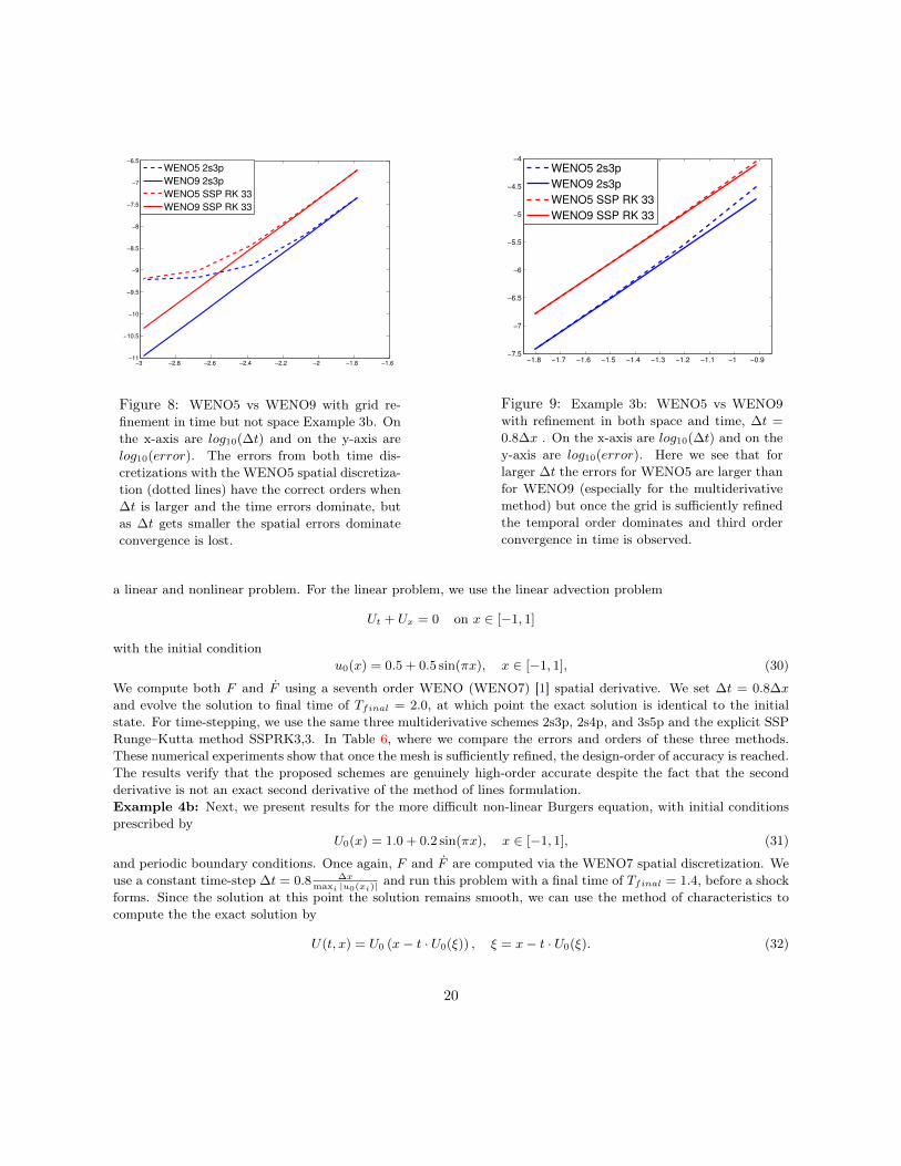
To see what happens if the spatial discretization errors dominate over the time errors, we compare two differentWENO spatial discretizations: the fifth order method WENO5 and the ninth order method WENO9. Here, weuse N = 301 points in space, and we choose ∆t = λ∆x for λ = 0.8, 0.6, 0.4, 0.2, 0.1, 0.05. We evolve the solution intime to Tf = 2.0 using the 2s3p and SSPRK3,3 methods. The log-log graph of the errors vs. ∆t is given in Figure8 We observe that the errors from both time discretizations with the WENO5 spatial discretization (dotted lines)have the correct orders when ∆t is larger and the time errors dominate, but as ∆t gets smaller the spatial errorsdominate convergence is lost. On the other hand, for the range of ∆t studied, the time-errors dominate over thespatial errors when using the highly accurate WENO9 (solid line) and so convergence is not lost. We note thatto see this behavior, the spatial approximation must be sufficiently accurate. In this case this is attained by using301 points in space and a high order spatial discretization. We also studied this problem with a co-refinement ofthe spatial and temporal grids, where we use ∆t = 0.8∆x for ∆x = 2π
N−1and N = 41, 81, 161, 321. Figure 9 shows
that while for larger ∆t the errors for WENO5 are larger than for WENO9, and this is more pronounced for themulti-derivative methods than for the explicit Runge–Kutta, once the grid is sufficiently refined the temporal errordominates and we see the third order convergence in time.
It is interesting to note that in all these studies the explicit SSP Runge–Kutta method SSPRK3,3 and thetwo-derivative method 2s3p behave similarly, indicating that the approximation of the second derivative does notplay a role in the loss of accuracy.Example 4: co-refinement of the spatial and temporal grids on linear advection with WENO7Example 4a: In this example, we compare the errors and order of convergence of the multiderivative methods on
19
−3 −2.8 −2.6 −2.4 −2.2 −2 −1.8 −1.6−11
−10.5
−10
−9.5
−9
−8.5
−8
−7.5
−7
−6.5
WENO5 2s3p
WENO9 2s3p
WENO5 SSP RK 33
WENO9 SSP RK 33
Figure 8: WENO5 vs WENO9 with grid re-finement in time but not space Example 3b. Onthe x-axis are log10(∆t) and on the y-axis arelog10(error). The errors from both time dis-cretizations with the WENO5 spatial discretiza-tion (dotted lines) have the correct orders when∆t is larger and the time errors dominate, butas ∆t gets smaller the spatial errors dominateconvergence is lost.
−1.8 −1.7 −1.6 −1.5 −1.4 −1.3 −1.2 −1.1 −1 −0.9−7.5
−7
−6.5
−6
−5.5
−5
−4.5
−4
WENO5 2s3p
WENO9 2s3p
WENO5 SSP RK 33
WENO9 SSP RK 33
Figure 9: Example 3b: WENO5 vs WENO9with refinement in both space and time, ∆t =
0.8∆x . On the x-axis are log10(∆t) and on they-axis are log10(error). Here we see that forlarger ∆t the errors for WENO5 are larger thanfor WENO9 (especially for the multiderivativemethod) but once the grid is sufficiently refinedthe temporal order dominates and third orderconvergence in time is observed.
a linear and nonlinear problem. For the linear problem, we use the linear advection problem
Ut + Ux = 0 on x ∈ [−1, 1]
with the initial conditionu0(x) = 0.5 + 0.5 sin(πx), x ∈ [−1, 1], (30)
We compute both F and F using a seventh order WENO (WENO7) [1] spatial derivative. We set ∆t = 0.8∆x
and evolve the solution to final time of Tfinal = 2.0, at which point the exact solution is identical to the initialstate. For time-stepping, we use the same three multiderivative schemes 2s3p, 2s4p, and 3s5p and the explicit SSPRunge–Kutta method SSPRK3,3. In Table 6, where we compare the errors and orders of these three methods.These numerical experiments show that once the mesh is sufficiently refined, the design-order of accuracy is reached.The results verify that the proposed schemes are genuinely high-order accurate despite the fact that the secondderivative is not an exact second derivative of the method of lines formulation.Example 4b: Next, we present results for the more difficult non-linear Burgers equation, with initial conditionsprescribed by
U0(x) = 1.0 + 0.2 sin(πx), x ∈ [−1, 1], (31)
and periodic boundary conditions. Once again, F and F are computed via the WENO7 spatial discretization. Weuse a constant time-step ∆t = 0.8 ∆x
maxi |u0(xi)|and run this problem with a final time of Tfinal = 1.4, before a shock
forms. Since the solution at this point the solution remains smooth, we can use the method of characteristics tocompute the the exact solution by
U(t, x) = U0 (x− t · U0(ξ)) , ξ = x− t · U0(ξ). (32)
20
SSPRK 3,3 2s3p 2s4p 3s5pλ error Order error Order error Order error Order
0.9 7.37× 10⁻⁶ — 1.71× 10⁻⁶ — 8.25× 10⁻⁸ — 1.24× 10⁻⁹ —0.8 5.24× 10⁻⁶ 2.89 1.22× 10⁻⁶ 2.89 5.21× 10⁻⁸ 3.89 6.99× 10⁻¹⁰ 4.89
0.7 3.44× 10⁻⁶ 3.14 7.99× 10⁻⁷ 3.14 3.00× 10⁻⁸ 4.14 3.52× 10⁻¹⁰ 5.14
0.6 2.18× 10⁻⁶ 2.96 5.08× 10⁻⁷ 2.96 1.63× 10⁻⁸ 3.96 1.64× 10⁻¹⁰ 4.96
0.5 1.27× 10⁻⁶ 2.98 2.94× 10⁻⁷ 2.98 7.89× 10⁻⁹ 3.98 6.61× 10⁻¹¹ 4.97
0.4 6.47× 10⁻⁷ 3.01 1.50× 10⁻⁷ 3.01 3.22× 10⁻⁹ 4.01 2.18× 10⁻¹¹ 4.97
Table 5: Convergence study for Example 3b, the linear advection problem with WENO9 differentiation ofthe spatial derivatives. Here we use N = 101 equidistant points between (0, 2π), and ∆t = λ∆x.
SSPRK 3,3 2s3p 2s4p 3s5pN error order error order error order error order41 3.00× 10−04 — 5.94× 10−05 — 7.54× 10−06 −−− 2.59× 10−06 —81 3.75× 10−05 3.00 7.39× 10−06 3.01 4.71× 10−07 4.00 8.03× 10−08 5.01
161 4.69× 10−06 3.00 9.23× 10−07 3.00 2.94× 10−08 4.00 2.51× 10−09 5.00
321 5.86× 10−07 3.00 1.15× 10−07 3.00 1.84× 10−09 4.00 7.82× 10⁻¹¹ 5.00
641 7.32× 10−08 3.00 1.44× 10−08 3.00 1.15× 10⁻¹⁰ 4.00 2.45× 10⁻¹² 5.00
1281 9.15× 10−09 3.00 1.80× 10−09 3.00 7.19× 10⁻¹² 4.00 7.75× 10⁻¹⁴ 4.98
Table 6: Convergence study for Example 4a: linear advection with WENO7 spatial differentiation andrefinement of both spatial and temporal grids. Here we use N points in space and ∆t = 0.8∆x. Thefour methods used to evolve the solution to time Tf = 2.0 are the explicit SSP Runge–Kutta methodSSPRK3,3 and the three multiderivative methods 2s3p, 2s4p, and 3s5p. Despite the fact that the secondderivative F is not the exact second derivative Ft, we still observe high-order accuracy for all methodsonce the grids are sufficiently refined.
SSPRK 3,3 2s3p 2s4p 3s5pN error order error order error order error order
161 3.09× 10−04 — 1.91× 10−04 — 1.58× 10−04 — 1.67× 10−04 —321 5.11× 10−05 2.60 2.00× 10−05 3.25 1.33× 10−05 3.57 1.76× 10−05 3.25
641 6.96× 10−06 2.88 1.70× 10−06 3.56 7.12× 10−07 4.22 9.34× 10−07 4.23
1281 8.80× 10−07 2.98 1.81× 10−07 3.23 3.38× 10−08 4.39 2.73× 10−08 5.09
2561 1.10× 10−07 3.00 2.22× 10−08 3.03 1.99× 10−09 4.09 7.49× 10⁻¹⁰ 5.19
5121 1.38× 10−08 3.00 2.76× 10−09 3.01 1.24× 10⁻¹⁰ 4.01 2.21× 10⁻¹¹ 5.08
10241 1.72× 10−09 3.00 3.44× 10⁻¹⁰ 3.00 7.75× 10⁻¹² 4.00 7.04× 10⁻¹³ 4.97
Table 7: Convergence study for Example 4b: Burgers’ equation with WENO7 spatial differentiation andrefinement of both spatial and temporal grids. Here we use N points in space and ∆t = 0.8∆x. Thefour methods used to evolve the solution to time Tf = 2.0 are the explicit SSP Runge–Kutta methodSSPRK3,3 and the three multiderivative methods 2s3p, 2s4p, and 3s5p. A more refined grid is needed inthis example compared to the linear example, but for a sufficiently refined grid we still observe high-orderaccuracy for all methods.
21
We solve for the implicit variable ξ using Netwon iteration with a tolerance of 10−14. The errors and order arepresented in Table 7. We see that it takes an even smaller mesh size than the linear problem before the errorsreach the asymptotic regime, but that once this happens we achieve the expected order. Again, these numericalexperiments further validate the fact that if the spatial error is not allowed to dominate, the high-order design-accuracy of the time discretization attained despite the fact that we do not directly differentiate the method oflines formulation to define the second derivative.
5 ConclusionsWith the increasing popularity of multi-stage multiderivative methods for use as time-stepping methods for hyper-bolic problems, the question of their strong stability properties needs to be addressed. In this work we presentedan SSP formulation for multistage two-derivative methods. We assumed that, in addition to the forward Eulercondition, the spatial discretization of interest satisfies a second derivative condition of the form (12). With theseassumptions in mind, we formulated an optimization problem which enabled us to find optimal explicit SSP multi-stage two-derivative methods of up to order five, thus breaking the SSP order barrier for explicit SSP Runge–Kuttamethods. Numerical test cases verify the convergence of these methods at the design-order, show that sharpnessof the SSP condition in many cases, and demonstrate the need for SSP time-stepping methods in simulationswhere the spatial discretization is specially designed to satisfy certain nonlinear stability properties. Future workwill involve building SSP multiderivative methods while assuming different base conditions (as in Remark 1) andwith higher derivatives. Additional work will involve developing new spatial discretizations suited for use withSSP multiderivative time stepping methods. These methods will be based on WENO or discontinuous Galerkinmethods and will satisfy pseudo-TVD and similar properties for systems of equations.
Acknowledgements This work was supported by: AFOSR grants FA9550-12-1-0224, FA9550-12-1-0343,FA9550-12-1-0455, FA9550-15-1-0282, and FA9550-15-1-0235; NSF grant DMS-1418804; New Mexico Consortiumgrant NMC0155-01; and NASA grant NMX15AP39G.
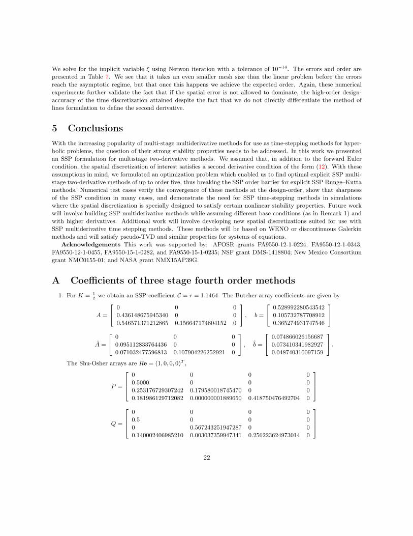
A Coefficients of three stage fourth order methods1. For K = 1
2we obtain an SSP coefficient C = r = 1.1464. The Butcher array coefficients are given by
A =
0 0 0
0.436148675945340 0 0
0.546571371212865 0.156647174804152 0
, b =
0.528992280543542
0.105732787708912
0.365274931747546
A =
0 0 0
0.095112833764436 0 0
0.071032477596813 0.107904226252921 0
, b =
0.074866026156687
0.073410341982927
0.048740310097159
.The Shu-Osher arrays are Re = (1, 0, 0, 0)T ,
P =
0 0 0 0
0.5000 0 0 0
0.253176729307242 0.179580018745470 0 0
0.181986129712082 0.000000001889650 0.418750476492704 0
Q =
0 0 0 0
0.5 0 0 0
0 0.567243251947287 0 0
0.140002406985210 0.003037359947341 0.256223624973014 0
22
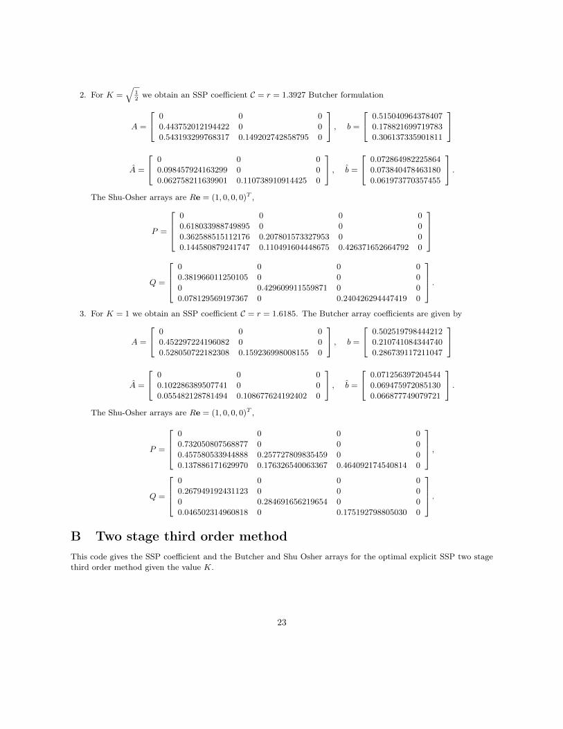
2. For K =√
12we obtain an SSP coefficient C = r = 1.3927 Butcher formulation
A =
0 0 0
0.443752012194422 0 0
0.543193299768317 0.149202742858795 0
, b =
0.515040964378407
0.178821699719783
0.306137335901811
A =
0 0 0
0.098457924163299 0 0
0.062758211639901 0.110738910914425 0
, b =
0.072864982225864
0.073840478463180
0.061973770357455
.The Shu-Osher arrays are Re = (1, 0, 0, 0)T ,
P =
0 0 0 0
0.618033988749895 0 0 0
0.362588515112176 0.207801573327953 0 0
0.144580879241747 0.110491604448675 0.426371652664792 0
Q =
0 0 0 0
0.381966011250105 0 0 0
0 0.429609911559871 0 0
0.078129569197367 0 0.240426294447419 0
.3. For K = 1 we obtain an SSP coefficient C = r = 1.6185. The Butcher array coefficients are given by
A =
0 0 0
0.452297224196082 0 0
0.528050722182308 0.159236998008155 0
, b =
0.502519798444212
0.210741084344740
0.286739117211047
A =
0 0 0
0.102286389507741 0 0
0.055482128781494 0.108677624192402 0
, b =
0.071256397204544
0.069475972085130
0.066877749079721
.The Shu-Osher arrays are Re = (1, 0, 0, 0)T ,
P =
0 0 0 0
0.732050807568877 0 0 0
0.457580533944888 0.257727809835459 0 0
0.137886171629970 0.176326540063367 0.464092174540814 0
,
Q =
0 0 0 0
0.267949192431123 0 0 0
0 0.284691656219654 0 0
0.046502314960818 0 0.175192798805030 0
.
B Two stage third order methodThis code gives the SSP coefficient and the Butcher and Shu Osher arrays for the optimal explicit SSP two stagethird order method given the value K.
23
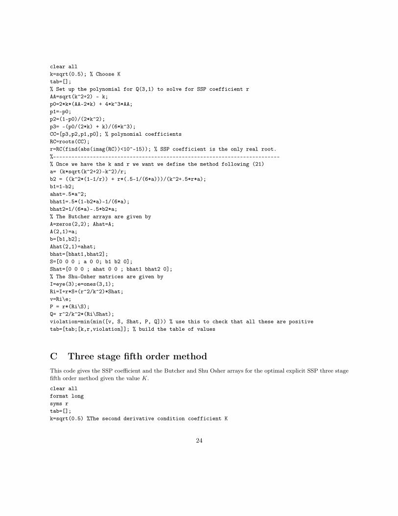
clear allk=sqrt(0.5); % Choose Ktab=[];% Set up the polynomial for Q(3,1) to solve for SSP coefficient rAA=sqrt(k^2+2) - k;p0=2*k*(AA-2*k) + 4*k^3*AA;p1=-p0;p2=(1-p0)/(2*k^2);p3= -(p0/(2*k) + k)/(6*k^3);CC=[p3,p2,p1,p0]; % polynomial coefficientsRC=roots(CC);r=RC(find(abs(imag(RC))<10^-15)); % SSP coefficient is the only real root.%--------------------------------------------------------------------------% Once we have the k and r we want we define the method following (21)a= (k*sqrt(k^2+2)-k^2)/r;b2 = ((k^2*(1-1/r)) + r*(.5-1/(6*a)))/(k^2+.5*r*a);b1=1-b2;ahat=.5*a^2;bhat1=.5*(1-b2*a)-1/(6*a);bhat2=1/(6*a)-.5*b2*a;% The Butcher arrays are given byA=zeros(2,2); Ahat=A;A(2,1)=a;b=[b1,b2];Ahat(2,1)=ahat;bhat=[bhat1,bhat2];S=[0 0 0 ; a 0 0; b1 b2 0];Shat=[0 0 0 ; ahat 0 0 ; bhat1 bhat2 0];% The Shu-Osher matrices are given byI=eye(3);e=ones(3,1);Ri=I+r*S+(r^2/k^2)*Shat;v=Ri\e;P = r*(Ri\S);Q= r^2/k^2*(Ri\Shat);violation=min(min([v, S, Shat, P, Q])) % use this to check that all these are positivetab=[tab;[k,r,violation]]; % build the table of values
C Three stage fifth order methodThis code gives the SSP coefficient and the Butcher and Shu Osher arrays for the optimal explicit SSP three stagefifth order method given the value K.
clear allformat longsyms rtab=[];k=sqrt(0.5) %The second derivative condition coefficient K
24
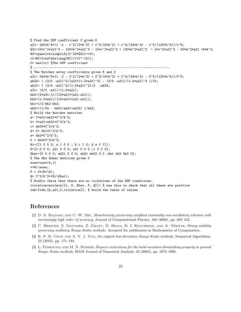
% Find the SSP coefficient C given Ka21= 240*k^6*(1 -r - r^2/(2*k^2) + r^3/(6*k^2) + r^4/(24*k^4) - r^5/(120*k^4))/r^6;Q31=10*r^2*a21^4 - 100*k^2*a21^3 - 10*r^2*a21^3 + 130*k^2*a21^2 + 3*r^2*a21^2 - 50*k^2*a21 +6*k^2;RC=vpasolve(simplify(r^22*Q31)==0);rr=RC(find(abs(imag(RC))<10^-15));C= max(rr) %The SSP coefficient% -------------------------------------------------------------------------% The Butcher array coefficients given K and Ca21= 240*k^6*(1 -C - C^2/(2*k^2) + C^3/(6*k^2) + C^4/(24*k^4) - C^5/(120*k^4))/C^6;ah32= ( (3/5 -a21)^2/(a21*(1-2*a21)^3) - (3/5 -a21)/(1-2*a21)^2 )/10;ah31= ( (3/5 -a21)^2/(1-2*a21)^2)/2 -ah32;a31= (3/5 -a21)/(1-2*a21);bh2=(2*a31-1)/(12*a21*(a31-a21));bh3=(1-2*a21)/(12*a31*(a31-a21));bh1=1/2-bh2-bh3;ah21=(1/24 - bh3*(ah31+ah32) )/bh2;% Build the Butcher matricesa= C*a21+ah21*C^2/k^2;b= C*a31+ah31*C^2/k^2;c= ah32*C^2/k^2;d= C+ bh1*C^2/k^2;e= bh2*C^2/k^2;f = bh3*C^2/k^2;Ri=([1 0 0 0; a 1 0 0 ; b c 1 0; d e f 1]);S=[0 0 0 0; a21 0 0 0; a31 0 0 0 ;1 0 0 0];Shat=[0 0 0 0; ah21 0 0 0; ah31 ah32 0 0 ;bh1 bh2 bh3 0];% The Shu Osher matrices given Ceone=ones(4,1)v=Ri\eone;P = C*(Ri\S);Q= C^2/k^2*(Ri\Shat);% Double check that there are no violations of the SSP conditions:violation=min(min([v, S, Shat, P, Q])) % use this to check that all these are positivetab=[tab;[k,a21,C,violation]]; % build the table of values
References[1] D. S. Balsara and C.-W. Shu, Monotonicity preserving weighted essentially non-oscillatory schemes with
increasingly high order of accuracy, Journal of Computational Physics, 160 (2000), pp. 405–452.
[2] C. Bresten, S. Gottlieb, Z. Grant, D. Higgs, D. I. Ketcheson, and A. Németh, Strong stabilitypreserving multistep Runge-Kutta methods. Accepted for publication in Mathematics of Computation.
[3] R. P. K. Chan and A. Y. J. Tsai, On explicit two-derivative Runge-Kutta methods, Numerical Algorithms,53 (2010), pp. 171–194.
[4] L. Ferracina and M. N. Spijker, Stepsize restrictions for the total-variation-diminishing property in generalRunge–Kutta methods, SIAM Journal of Numerical Analysis, 42 (2004), pp. 1073–1093.
25
[5] , An extension and analysis of the Shu–Osher representation of Runge–Kutta methods, Mathematics ofComputation, 249 (2005), pp. 201–219.
[6] E. Gekeler and R. Widmann, On the order conditions of Runge-Kutta methods with higher derivatives,Numer. Math., 50 (1986), pp. 183–203.
[7] S. Gottlieb, D. I. Ketcheson, and C.-W. Shu, Strong Stability Preserving Runge–Kutta and MultistepTime Discretizations, World Scientific Press, 2011.
[8] Z. J. Grant, Explicit SSP multistage two-derivative SSP optimization code. https://github.com/SSPmethods/SSPMultiStageTwoDerivativeMethods, February 2015.
[9] A. Harten, B. Engquist, S. Osher, and S. R. Chakravarthy, Uniformly high-order accurate essentiallynonoscillatory schemes. III, J. Comput. Phys., 71 (1987), pp. 231–303.
[10] J. Hesthaven, S. Gottlieb, and D. Gottlieb, Spectral methods for time dependent problems, CambridgeMonographs of Applied and Computational Mathematics, Cambridge University Press, 2007.
[11] I. Higueras, On strong stability preserving time discretization methods, Journal of Scientific Computing, 21(2004), pp. 193–223.
[12] , Representations of Runge–Kutta methods and strong stability preserving methods, SIAM Journal OnNumerical Analysis, 43 (2005), pp. 924–948.
[13] G.-S. Jiang and C.-W. Shu, Efficient implementation of weighted ENO schemes, J. Comput. Phys., 126(1996), pp. 202–228.
[14] K. Kastlunger and G. Wanner, On Turan type implicit Runge-Kutta methods, Computing (Arch. Elek-tron. Rechnen), 9 (1972), pp. 317–325. 10.1007/BF02241605.
[15] K. H. Kastlunger and G. Wanner, Runge Kutta processes with multiple nodes, Computing (Arch. Elek-tron. Rechnen), 9 (1972), pp. 9–24.
[16] D. I. Ketcheson, Highly efficient strong stability preserving Runge–Kutta methods with low-storage imple-mentations, SIAM Journal on Scientific Computing, 30 (2008), pp. 2113–2136.
[17] D. I. Ketcheson, S. Gottlieb, and C. B. Macdonald, Strong stability preserving two-step Runge-Kuttamethods, SIAM Journal on Numerical Analysis, (2012), pp. 2618–2639.
[18] D. I. Ketcheson, C. B. Macdonald, and S. Gottlieb, Optimal implicit strong stability preservingRunge–Kutta methods, Applied Numerical Mathematics, 52 (2009), p. 373.
[19] D. I. Ketcheson, M. Parsani, and A. J. Ahmadia, Rk-opt: Software for the design of Runge–Kuttameththods, version 0.2. https://github.com/ketch/RK-opt.
[20] J. F. B. M. Kraaijevanger, Contractivity of Runge–Kutta methods, BIT, 31 (1991), pp. 482–528.
[21] P. Lax and B. Wendroff, Systems of conservation laws, Communications in Pure and Applied Mathemat-ics, 13 (1960), pp. 217–237.
[22] T. Mitsui, Runge-Kutta type integration formulas including the evaluation of the second derivative. i., Publ.Res. Inst. Math. Sci., 18 (1982), pp. 325–364.
[23] T. Nguyen-Ba, H. Nguyen-Thu, T. Giordano, and R. Vaillancourt, One-step strong-stability-preserving Hermite-Birkhoff-Taylor methods, Scientific Journal of Riga Technical University, 45 (2010), pp. 95–104.
[24] N. Obreschkoff, Neue Quadraturformeln, Abh. Preuss. Akad. Wiss. Math.-Nat. Kl., 4 (1940).
[25] H. Ono and T. Yoshida, Two-stage explicit Runge-Kutta type methods using derivatives., Japan J. Indust.Appl. Math., 21 (2004), pp. 361–374.
26
[26] J. Qiu, M. Dumbser, and C.-W. Shu, The discontinuous Galerkin method with Lax–Wendroff type timediscretizations, Computer Methods in Applied Mechanics and Engineering, 194 (2005), pp. 4528–4543.
[27] J. Qiu and C.-W. Shu, Finite Difference WENO schemes with Lax–Wendroff-type time discretizations,SIAM Journal on Scientific Computing, 24 (2003), pp. 2185–2198.
[28] S. J. Ruuth and R. J. Spiteri, Two barriers on strong-stability-preserving time discretization methods,Journal of Scientific Computation, 17 (2002), pp. 211–220.
[29] D. C. Seal, Y. Guclu, and A. J. Christlieb, High-order multiderivative time integrators for hyperbolicconservation laws, Journal of Scientific Computing, 60 (2014), pp. 101–140.
[30] H. Shintani, On one-step methods utilizing the second derivative, Hiroshima Mathematical Journal, 1 (1971),pp. 349–372.
[31] , On explicit one-step methods utilizing the second derivative, Hiroshima Mathematical Journali, 2 (1972),pp. 353–368.
[32] C.-W. Shu, Total-variation diminishing time discretizations, SIAM J. Sci. Stat. Comp., 9 (1988), pp. 1073–1084.
[33] C.-W. Shu and S. Osher, Efficient implementation of essentially non-oscillatory shock-capturing schemes,Journal of Computational Physics, 77 (1988), pp. 439–471.
[34] R. J. Spiteri and S. J. Ruuth, A new class of optimal high-order strong-stability-preserving time discretiza-tion methods, SIAM J. Numer. Anal., 40 (2002), pp. 469–491.
[35] D. D. Stancu and A. H. Stroud, Quadrature formulas with simple Gaussian nodes and multiple fixednodes, Math. Comp., 17 (1963), pp. 384–394.
[36] E. Toro and V. Titarev, Solution of the generalized Riemann problem for advection–reaction equations,Proceedings of the Royal Society of London A: Mathematical, Physical and Engineering Sciences, 458 (2002),pp. 271–281.
[37] A. Y. J. Tsai, R. P. K. Chan, and S. Wang, Two-derivative Runge–Kutta methods for PDEs using anovel discretization approach, Numerical Algorithms, 65 (2014), pp. 687–703.
[38] P. Turán, On the theory of the mechanical quadrature, Acta Sci. Math. Szeged, 12 (1950), pp. 30–37.
27