arX

iv:0

811.

2053

v1 [

astr

o-ph

] 13

Nov

200

8

©November 13, 2008

Physi al properties of galaxies and their evolutionin the VIMOS VLT Deep Survey⋆I. The evolution of the mass-metalli ity relation up to z∼ 0.9

F. Lamareille1,3, J. Brinchmann19, T. Contini1, C.J. Walcher7, S. Charlot10,8, E. Pérez-Montero1, G. Zamorani3, L.Pozzetti3, M. Bolzonella3, B. Garilli2, S. Paltani15,16, A. Bongiorno22, O. Le Fèvre7, D. Bottini2, V. Le Brun7, D.

Maccagni2, R. Scaramella4,13, M. Scodeggio2, L. Tresse7, G. Vettolani4, A. Zanichelli4, C. Adami, S. Arnouts23,7, S.Bardelli3, A. Cappi3, P. Ciliegi3, S. Foucaud21, P. Franzetti2, I. Gavignaud12, L. Guzzo9, O. Ilbert20, A. Iovino9, H.J.McCracken10,11, B. Marano6, C. Marinoni18, A. Mazure7, B. Meneux22,24, R. Merighi3, R. Pellò1, A. Pollo7,17, M.

Radovich5, D. Vergani2, E. Zucca3, A. Romano5, A. Grado5, and L. Limatola5

(Affiliations can be found after the references)

Preprint online version: November 13, 2008Abstra tAims. We want to derive the mass-metallicity relation of star-forming galaxies up toz∼ 0.9, using data from the VIMOS VLT Deep Survey. Themass-metallicity relation is commonly understood as the relation between the stellar mass and the gas-phase oxygen abundance.Methods. Automatic measurement of emission-line fluxes and equivalent widths have been performed on the full spectroscopic sampleof the VIMOS VLT Deep Survey. This sample is divided into two sub-samples depending on the apparent magnitude selection:wide (IAB < 22.5)and deep (IAB < 24). These two samples span two different ranges of stellar masses. Emission-line galaxies have been separated into star-forming galaxies and active galactic nuclei using emissionline ratios. For the star-forming galaxies the emission line ratios have also beenused to estimate gas-phase oxygen abundance, using empirical calibrations renormalized in order to give consistent results at low and highredshifts. The stellar masses have been estimated by fittingthe whole spectral energy distributions with a set of stellar population synthesis models.Results. We assume at first order that the shape of the mass-metallicity relation remains constant with redshift. Then we find a strongermetallicity evolution in the wide sample as compared to the deep sample. We thus conclude that the mass-metallicity relation is flatter at higherredshift. At z∼ 0.77, galaxies at 109.4 solar masses have−0.18 dex lower metallicities than galaxies of similar masses in the local universe,while galaxies at 1010.2 solar masses have−0.28 dex lower metallicities. By comparing the mass-metallicity and luminosity-metallicity relations,we also find an evolution in mass-to-light ratios: galaxies at higher redshifts being more active. The observed flattening of the mass-metallicityrelation at high redshift is analyzed as an evidence in favorof the open-closed model.Key words. galaxies: evolution – galaxies: fundamental parameters – galaxies: abundances – galaxies: starburst1. Introdu tionThe stellar mass and the gas-phase metallicity of a galaxy aretwo of the main parameters involved in the study of galaxy for-mation and evolution. As cosmological time progresses, theorypredicts that both the mean metallicity and stellar mass of galax-ies increase with age as galaxies undergo chemical enrichmentand grow through merging processes. At any given epoch, theaccumulated history of star formation, gas inflows and outflows,affects a galaxy mass and its metallicity. Hence one expectsthe-ses quantities to show some correlation and this will provide cru-cial information about the physical processes that govern galaxyformation.

First discovered for irregular galaxies (Lequeux et al.1979), the mass-metallicity relation has been intensivelystudied (Skillman et al. 1989; Brodie & Huchra 1991;

⋆ based on data obtained with the European Southern ObservatoryVery Large Telescope, Paranal, Chile, program 070.A-9007(A), and ondata obtained at the Canada-France-Hawaii Telescope, operated by theCNRS in France, CNRC in Canada and the University of Hawaii.

Zaritsky et al. 1994; Richer & McCall 1995; Garnett et al.1997; Pilyugin & Ferrini 2000, among others) and is now wellestablished in the local universe by the work of Tremonti et al.(2004) with SDSS data and Lamareille et al. (2004) with 2dF-GRS data, the latter done on the luminosity-metallicity relationwhich is easier to derive when small number of photometricbands are available. These two studies have shown in twodifferent ways that the mass-metallicity relation is mainly drivenby the decrease of metal loss when stellar mass increases.Tremonti et al. (2004) have indeed observed an increase ofthe effective yield with stellar mass, while Lamareille et al.(2004) have shown the increase of the slope of the luminosity-metallicity relation. This last trend has also been observeddown to much lower galaxy masses by Lee et al. (2006). Wenevertheless note that they also observe a large scatter in theeffective yield, which they find difficult to analyse in the contextof more efficient mass loss among low mass galaxies.

Hierarchical galaxy formation models, that take into accountthe chemical evolution and feedback processes, are able to repro-duce the observed mass-metallicity relation in the local universe

∼

(e.g. De Lucia et al. 2004; de Rossi et al. 2007; Finlator & Davé2008). However these models rely on free parameters, such asfeedback efficiency, which are not yet well constrained by ob-servations. Alternative scenarios have been proposed to explainthe mass-metallicity relation including low star formation ef-ficiency in low-mass galaxies caused by supernova feedback(Brooks et al. 2007) and a variable stellar initial mass func-tion being more top-heavy in galaxies with higher star forma-tion rates, thereby producing higher metal yields (Köppen et al.2007).

The evolution of the mass-metallicity relation on cosmo-logical timescales is now predicted by semi-analytic models ofgalaxy formation, that include chemical hydrodynamic simula-tions within the standardΛ-CDM framework (De Lucia et al.2004; Davé & Oppenheimer 2007). Reliable observational es-timates of the mass-metallicity relation of galaxies at differentepochs (and hence different redshifts) may thus provide impor-tant constraints on galaxy evolution scenarios. Estimatesof themass-metallicity - or luminosity-metallicity - relation of galax-ies up toz∼ 1 are limited so far to small samples (Hammer et al.2005; Liang et al. 2004; Maier et al. 2004; Kobulnicky et al.2003; Maier et al. 2005, among others). Recent studies havebeen performed on larger samples (> 100 galaxies) but withcontradictory results. Savaglio et al. (2005) concluded with asteeper slope in the distant universe, interpreting these resultsin the framework of the closed-box model. On the contrary,Lamareille et al. (2006a) did not find any significant evolutionof the slope of the luminosity-metallicity relation, whilethe av-erage metallicity atz≈ 0.9 is lowered by 0.55 dex at a givenluminosity, and by 0.28 dex after correction for luminosityevolution. Shapley et al. (2005) and Liu et al. (2008) have alsofound 0.2− 0.3 dex lower metallicities atz = 1in the DEEP2sample. At higher redshifts Erb et al. (2006) derived a mass-metallicity relation atz∼ 2 lowered by 0.3 dex in metallicitycompared with the local estimate, a trend which could extendup toz∼ 3.3 (Maiolino et al. 2007). Please note that the abovenumbers are given after the metallicities have been renormal-ized to the same reference calibration in order to be comparable(Kewley & Ellison 2008).

In this work, we present the first attempt to derive the mass-metallicity relation at different epochs up toz∼ 1 using a unique,large (almost 20 000 galaxies) and homogeneous sample ofgalaxies selected in the VIMOS VLT Deep Survey (VVDS). Thepaper is organized as follows: the sample selection is describedin Sect. 2, the estimation of stellar masses and magnitudes fromSED fitting are described in Sect. 3, the estimation of metal-licities from line ratios is described in Sec. 4, and we finallystudy the luminosity-metallicity (Sect. 5), and mass-metallicity(Sect. 6) relations. Throughout this paper we normalize thede-rived stellar masses, and absolute magnitudes, with the stan-dardΛ-CDM cosmology, i.e.h = 0.7, Ωm = 0.3 andΩΛ = 0.7(Spergel et al. 2003).2. Des ription of the sampleThe VIMOS VLT Deep Survey (VVDS, Le Fèvre et al. 2003b)is one of the widest and deepest spectrophotometric surveysof distant galaxies with a mean redshift ofz ≈ 0.7. Theoptical spectroscopic data, obtained with the VIsible Multi-Object Sectrograph (VIMOS, Le Fèvre et al. 2003a) installedatESO/VLT (UT3), offers a great opportunity to study the evo-lution of the mass-metallicity relation on a statisticallysignif-icant sample up toz≈ 0.9. This limitation is imposed, in thecurrent study, by the bluest emission lines needed to compute a

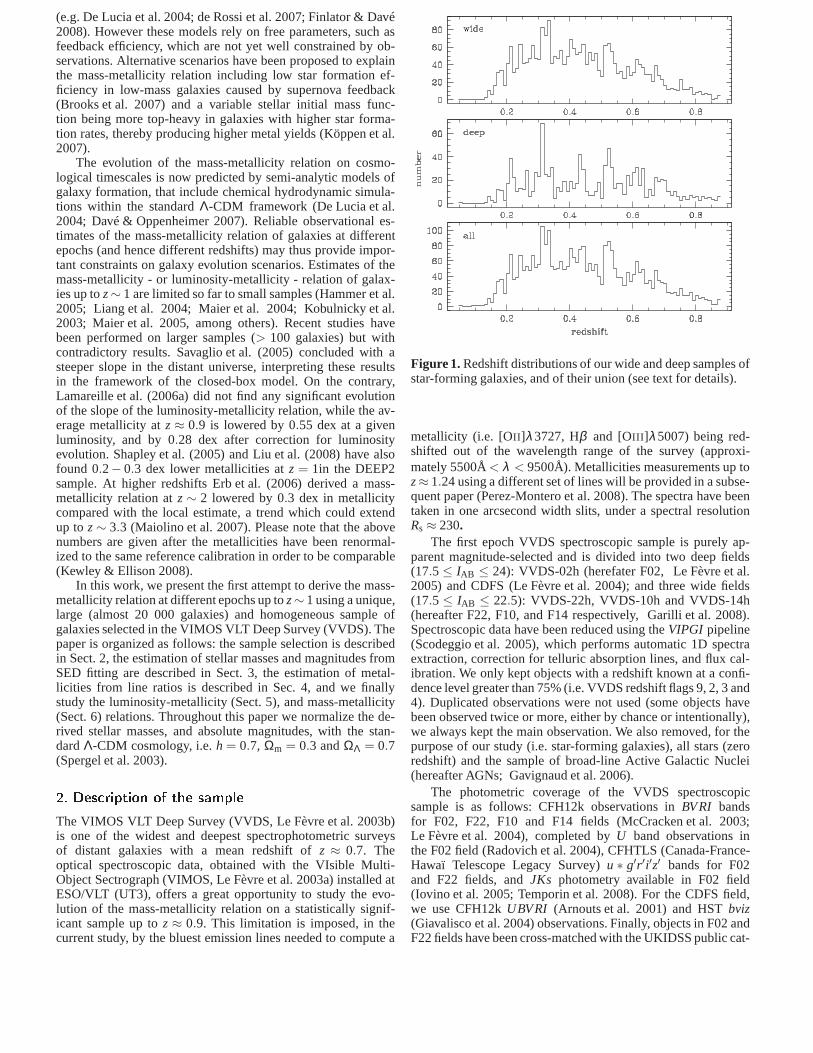
Figure 1.Redshift distributions of our wide and deep samples ofstar-forming galaxies, and of their union (see text for details).

metallicity (i.e. [OII ]λ3727, Hβ and [OIII ]λ5007) being red-shifted out of the wavelength range of the survey (approxi-mately 5500Å< λ < 9500Å). Metallicities measurements up toz≈ 1.24 using a different set of lines will be provided in a subse-quent paper (Perez-Montero et al. 2008). The spectra have beentaken in one arcsecond width slits, under a spectral resolutionRs ≈ 230.

The first epoch VVDS spectroscopic sample is purely ap-parent magnitude-selected and is divided into two deep fields(17.5 ≤ IAB ≤ 24): VVDS-02h (herefater F02, Le Fèvre et al.2005) and CDFS (Le Fèvre et al. 2004); and three wide fields(17.5 ≤ IAB ≤ 22.5): VVDS-22h, VVDS-10h and VVDS-14h(hereafter F22, F10, and F14 respectively, Garilli et al. 2008).Spectroscopic data have been reduced using theVIPGI pipeline(Scodeggio et al. 2005), which performs automatic 1D spectraextraction, correction for telluric absorption lines, andflux cal-ibration. We only kept objects with a redshift known at a confi-dence level greater than 75% (i.e. VVDS redshift flags 9, 2, 3 and4). Duplicated observations were not used (some objects havebeen observed twice or more, either by chance or intentionally),we always kept the main observation. We also removed, for thepurpose of our study (i.e. star-forming galaxies), all stars (zeroredshift) and the sample of broad-line Active Galactic Nuclei(hereafter AGNs; Gavignaud et al. 2006).

The photometric coverage of the VVDS spectroscopicsample is as follows: CFH12k observations inBVRI bandsfor F02, F22, F10 and F14 fields (McCracken et al. 2003;Le Fèvre et al. 2004), completed byU band observations inthe F02 field (Radovich et al. 2004), CFHTLS (Canada-France-Hawaï Telescope Legacy Survey)u ∗ g′r ′i′z′ bands for F02and F22 fields, andJKs photometry available in F02 field(Iovino et al. 2005; Temporin et al. 2008). For the CDFS field,we use CFH12kUBVRI (Arnouts et al. 2001) and HSTbviz(Giavalisco et al. 2004) observations. Finally, objects inF02 andF22 fields have been cross-matched with the UKIDSS public cat-

∼

alog (Warren et al. 2007), providing additional observations inJK bands.

Throughout this paper, we will use adeepand awidesam-ples. The deep sample is made of F02 and CDFS fields. Upto z < 1.4 (the limit for the [OII ]λ3727 emission line to be inthe observed wavelength range), the deep sample contains 7404galaxies (non-broad-line AGN) with a redshift measured at aconfidence level greater than 75%. The wide sample is madeof F22, F10, F14, F02 and CDFS fields (the last two being lim-ited out toIAB ≤ 22.5). Up toz< 1.4 the wide sample contains13978 galaxies (non-broad-line AGN) with a redshift measuredat a confidence level greater than 75%. We draw the reader’sattention on the fact that the two samples overlap for galaxiesobserved in F02 or CDFS fields atIAB ≤ 22.5, giving a totalnumber of 18648 galaxies. Fig. 1 shows the redshift distributionof the star-forming galaxies (see Sect. 2.2) in the wide and deepsamples and in their union.2.1. Automati spe tral measurementsThe emission lines fluxes and equivalent widths, in all VVDSgalaxy (non-broad-line AGN) spectra, have been measuredwith the platefit_vimospipeline. Originally developed for thehigh spectral resolution SDSS spectra (Tremonti et al. 2004;Brinchmann et al. 2004), theplatefit software has first beenadapted to fit accurately all emission lines after removing thestellar continuum and absorption lines from lower resolution andlower signal-to-noise spectra (Lamareille et al. 2006b). Finally,other improvements have been made to the newplatefit_vimospipeline thanks to tests performed on the VVDS and zCOSMOS(Lilly et al. 2006) spectroscopic samples. A full discussion ofplatefit_vimospipeline will be presented in Lamareille et al. (inpreparation) but, for the benefit of the reader, we outline some ofthe main features in this section.

The stellar component of the spectra is fitted as a non-negative linear combination of 30 single stellar population tem-plates with different ages (0.005, 0.025, 0.10, 0.29, 0.64, 0.90,1.4, 2.5, 5 and 11Gyr) and metallicities (0.2, 1 and 2.5 Z⊙).These templates have been derived using the Bruzual & Charlot(2003) library and resampled to the velocity dispersion of VVDSspectra. The dust attenuation in the stellar population model isleft as a free parameter. Foreground dust attenuation from theMilky Way has been corrected using Schlegel et al. (1998) maps.

After removal of the stellar component, the emission linesare fitted together as a singlenebular spectrummade of a sumof gaussians at specified wavelengths. All emission lines aretied to have the same width, with exception of the [OII ]λ3727line which is actually a doublet of two lines at 3726 and3729 Å and appear broadened compared to the other singlelines. The spectral resolution is also too low to clearly separate[N II ]λ6584 and Hα emission lines. It has been shown howeverby Lamareille et al. (2006b) that the [NII ]λ6584/Hα emission-line ratio, which is used as a metallicity calibrator, can bereli-ably measured above a sufficient signal-to-noise ratio evenat theresolution of VVDS.

Note that because of the limited observed wavelength cover-age of the spectra, we do not observe all well-known optical linesat all redshifts. Thanks to the stellar-part subtraction, no correc-tion for underlying absorption has to be applied to the Balmeremission lines.

The error spectrum which is needed for both fits of the stellaror nebular components is calculated as follows: a first guessisobtained from photons statistics and sky subtraction and iscalcu-

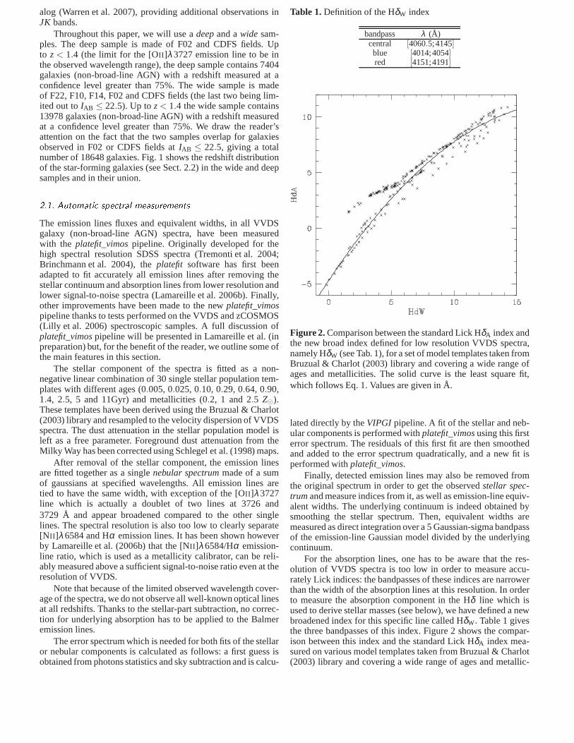
Table 1.Definition of the HδW index

bandpass λ (Å)central [4060.5;4145]blue [4014;4054]red [4151;4191]

Figure 2.Comparison between the standard Lick HδA index andthe new broad index defined for low resolution VVDS spectra,namely HδW (see Tab. 1), for a set of model templates taken fromBruzual & Charlot (2003) library and covering a wide range ofages and metallicities. The solid curve is the least square fit,which follows Eq. 1. Values are given in Å.

lated directly by theVIPGI pipeline. A fit of the stellar and neb-ular components is performed withplatefit_vimosusing this firsterror spectrum. The residuals of this first fit are then smoothedand added to the error spectrum quadratically, and a new fit isperformed withplatefit_vimos.

Finally, detected emission lines may also be removed fromthe original spectrum in order to get the observedstellar spec-trumand measure indices from it, as well as emission-line equiv-alent widths. The underlying continuum is indeed obtained bysmoothing the stellar spectrum. Then, equivalent widths aremeasured as direct integration over a 5 Gaussian-sigma bandpassof the emission-line Gaussian model divided by the underlyingcontinuum.

For the absorption lines, one has to be aware that the res-olution of VVDS spectra is too low in order to measure accu-rately Lick indices: the bandpasses of these indices are narrowerthan the width of the absorption lines at this resolution. Inorderto measure the absorption component in the Hδ line which isused to derive stellar masses (see below), we have defined a newbroadened index for this specific line called HδW. Table 1 givesthe three bandpasses of this index. Figure 2 shows the compar-ison between this index and the standard Lick HδA index mea-sured on various model templates taken from Bruzual & Charlot(2003) library and covering a wide range of ages and metallic-

∼

Table 2.Sets of emission lines which are required to haveS/N >4 in various redshift ranges associated to the various diagnosticsused in this study.

Redshift [OII ] Hβ [OIII ] Hα [N II ] [SII ]0.0 < z< 0.2 X X X

0.2 < z< 0.4 X X X X⋆

X⋆

0.4 < z< 0.5 X X

0.5 < z< 0.9 X X X

⋆ For the red diagnostic the [NII ]λ6584 and [SII ]λλ6717+6731 emis-sion lines may not be used at the same time.

Figure 4. Blue spectral classification of 1060 narrow emission-line galaxies in the redshift bin 0.5 < z< 0.9. The emission-lineratios – i.e. [OIII ]λ5007/Hβ and [OII ]λ3727/Hβ – are calcu-lated using equivalent widths. The red solid curve is the empir-ical separation defined by Lamareille et al. (2004). The dashedcurves delimits the error domain where both star-forming andAGNs galaxies show similar blue line ratios. The star-forminggalaxies are plotted as blue triangles, the Seyfert 2 galaxies asgreen solid squares, the candidate star-forming galaxies as redsolid pentagons, and the candidate AGNs as orange open pen-tagons. The error bars are shown in grey.

ities. For future comparison purpose between VVDS measure-ments and other studies, we derive the following relation:

HδA = −4.69+1.691×HδW−0.044711×Hδ 2W (1)

Note that the majority of points lying outside the fitted re-lation in Fig. 2 (for HδW < 5Å) are models with a very youngstellar population (< 10 Myr), hence this relation is only validfor stellar populations older than 10 Myr.2.2. Sele tion of star-forming galaxies2.2.1. Des ription of the various diagnosti sTo ensure accurate abundance determinations, we restrict ourattention to galaxies with emission lines detected atS/N > 4,where the set of lines considered for this S/N cut varies with

redshift. Table 2 provides a summary of the emission lines re-quired to haveS/N > 4 in the various redshift ranges associatedto the various diagnostics defined below.

Our work intends to understand the star-formation process ingalaxies. Thus we have to remove from the sample of emission-line galaxies those for which the source of ionized gas, respon-sible for these lines, is not hot young stars. Emission-linegalax-ies can be classified in various spectral types, which dependonthe nature of their nebular spectrum. The two main categoriesare the star-forming and AGN galaxies. Their source of ionizingphotons are respectively hot young stars, or the accretion diskaround a massive black-hole. As stated before, broad-line AGNs(also called Seyfert 1 galaxies) are already taken out of oursam-ple. The narrow-line AGNs are divided in two sub-categories:Seyfert 2 galaxies , and LINERs .

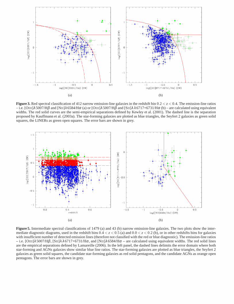
Both Seyfert 2 galaxies and LINERs can be distinguishedfrom star-forming galaxies using standard diagnostic diagrams(Baldwin et al. 1981; Veilleux & Osterbrock 1987), which arebased on emission-line ratios. The most commonly used classi-fication is provided by the [OIII ]λ5007/Hβ vs. [NII ]λ6584/Hαdiagram (Fig. 3a), for which a semi-empirical limit betweenstar-forming, Seyfert 2 galaxies, and LINERs has been de-rived by Kewley et al. (2001) from photo-ionization models.Due to our low spectral resolution, the [NII ]λ6584 line is notalways detected and its detection is less reliable than otherlines, because of possible deblending problems with the brightHα line. Consequently, most of the galaxies in the same red-shift range are actually classified with the [OIII ]λ5007/Hβ vs.[SII ]λ λ6717+6731/Hα diagram (see Fig. 3b).

The two diagrams shown in Fig. 3, which we also refer toas the red diagnostics, can only be used with our data in the0.2< z< 0.4 redshift range, as the desired emission lines are notvisible outside this domain. At higher redshifts, one can use thealternative blue diagnostic which was empirically calibrated byLamareille et al. (2004) from 2dFGRS data, in order to give sim-ilar results as the red diagnostics. The blue diagnostic is basedon the [OIII ]λ5007/Hβ vs. [OII ]λ3727/Hβ diagram (line ratioscalculated on rest-frame equivalent widths), and may be appliedin the 0.5 < z< 0.9 redshift range (see Fig. 4).

For the other redshift ranges, where neither the red nor theblue diagnostic applies, we use a minimal classification based onHα, [NII ]λ6584 and [SII ]λ λ6717+6731 for 0.0 < z< 0.2, andon Hβ and [OIII ]λ5007 for 0.4 < z< 0.5. We propose the fol-lowing selection (called Hβ diagnostic) for star-forming galax-ies in the 0.4 < z< 0.5 redshift range: log([Oiii]λ5007/Hβ ) <0.6 (rest-frame equivalent widths, see Fig. 5a). We note that realstar-forming galaxies which are lost with the Hβ diagnostic aremainly low metallicity ones. In any case a quick check on SDSSdata has told us that no more than 40% of star-forming galax-ies with 12+ log(O/H) < 8.1 actually fall in the AGN regionof the Hβ diagnostic, this proportion being negligible at highermetallicities.

Figure 5b shows the minimum classification for the 0.0 <z< 0.2 redshift range (called Hα diagnostic). The proposed sep-aration has been derived based on the 2dFGRS data (Lamareille2006) and follows the equation (rest-frame equivalent widths):

log([Nii]λ6584/Hα) =

−0.4 if log([Sii]λ λ6717+6731/Hα)≥−0.3−0.7−1.05log([Sii]λ λ6717+6731/Hα) otw.

(2)

This equation have been derived to efficiently reduce boththe contamination by real AGNs in the star-forming galaxiesre-gion (< 1%), and the fraction of real star-forming galaxies whichare lost (< 4%).

∼

(a) (b)

Figure 3. Red spectral classification of 412 narrow emission-line galaxies in the redshift bin 0.2< z< 0.4. The emission-line ratios– i.e. [OIII ]λ5007/Hβ and [NII ]λ6584/Hα (a) or [OIII ]λ5007/Hβ and [SII ]λ λ6717+6731/Hα (b) – are calculated using equivalentwidths. The red solid curves are the semi-empirical separations defined by Kewley et al. (2001). The dashed line is the separationproposed by Kauffmann et al. (2003a). The star-forming galaxies are plotted as blue triangles, the Seyfert 2 galaxies asgreen solidsquares, the LINERs as green open squares. The error bars areshown in grey.

(a) (b)

Figure 5. Intermediate spectral classifications of 1479 (a) and 43 (b)narrow emission-line galaxies. The two plots show the inter-mediate diagnostic diagrams, used in the redshift bins 0.4 < z< 0.5 (a) and 0.0 < z< 0.2 (b), or in other redshifts bins for galaxieswith insufficient number of detected emission lines (therefore not classified with the red or blue diagnostic). The emission-line ratios– i.e. [OIII ]λ5007/Hβ , [SII ]λ λ6717+6731/Hα, and [NII ]λ6584/Hα – are calculated using equivalent widths. The red solid linesare the empirical separations defined by Lamareille (2006).In the left panel, the dashed lines delimits the error domainwhere bothstar-forming and AGNs galaxies show similar blue line ratios. The star-forming galaxies are plotted as blue triangles,the Seyfert 2galaxies as green solid squares, the candidate star-forming galaxies as red solid pentagons, and the candidate AGNs as orange openpentagons. The error bars are shown in grey.

∼

Table 3.Statistics of star-forming galaxies and narrow-line AGNs among emission-line galaxies for various diagnostics dependingon which emission lines are observed (see text for details).The results are presented for the two wide and deep samples used inthis paper, and for their union (some objects are in common).We also mention for each sample the total number of objects whichincludes emission-line, faint and early-type galaxies.

Sample/Diagnostic red % blue % Hα % Hβ % all %wide (13978)emission-line (total) 455 100 924 100 47 100 1402 100 2828 100star-forming 415 91 768 83 30 64 978 70 2191 77candidate s.-f. 0 0 103 11 0 0 306 22 409 14candidate AGN 0 0 35 4 0 0 74 5 109 4Seyfert 2 18 4 18 2 17 36 44 3 97 3LINER 22 5 0 0 0 0 0 0 22 1

deep(7404)emission-line (total) 151 100 568 100 11 100 574 100 1304 100star-forming 136 90 412 73 10 91 312 54 870 67candidate s.-f. 0 0 92 16 0 0 166 29 258 20candidate AGN 0 0 47 8 0 0 47 8 94 7Seyfert 2 5 3 17 3 1 9 49 9 72 6LINER 10 7 0 0 0 0 0 0 10 1

union of wide and deep(18648)emission-line (total) 469 100 1213 100 47 100 1671 100 3400 100star-forming 427 91 945 78 30 64 1074 64 2476 73candidate s.-f. 0 0 166 14 0 0 404 24 570 17candidate AGN 0 0 70 6 0 0 111 7 181 5Seyfert 2 20 4 32 3 17 36 82 5 151 4LINER 22 5 0 0 0 0 0 0 22 1

The results of all diagnostics, in the wide, deep, and globalsamples, are shown in Table. 3.2.2.2. Dis ussion of possible biasesIt is very important to evaluate the possible sources of biases,which may affect the spectral classification, coming from theuse of various diagnostics at different redshift ranges.

As the [OII ]λ3727/Hβ line ratio is less accurate than[N II ]λ6584/Hα, or [SII ]λ λ6717+6731/Hα, to distinguish be-tween star-forming and Seyfert 2 galaxies, the blue diagnostic isdefined with an error domain (see the dashed curves in Fig. 4),inside which individual galaxies cannot be safely classified. Wethus introduce two new categories of galaxies: candidate star-forming galaxies and candidate AGNs, which fall respectivelyin the lower-half or the upper-half part of the error domain.

We know however that AGNs are in minority in the universe.Thus we emphasize thati) still no reliable classification can beperformed for any individual galaxy falling inside the error do-main of the blue diagnostic,ii) the search for AGNs is highlycontaminated in the candidate AGN region,but iii) any studyinvolving statistically significant samples of star-forming galax-ies should not be biased when candidate star-forming galaxiesand candidate AGNs are included. As it will be shown in Sect. 5and 6, this ends up to a negligible bias on the derived metallici-ties.

As for the blue diagnostic, we have defined an error do-main for the Hβ diagnostic in the following range: 0.4 <log([Oiii]λ5007/Hβ ) < 0.6. Star-forming galaxies or AGNsfalling inside this domain are classified as candidates.

One can see in Table. 3 that the red diagnostic is the only oneable to find LINERs. Indeed, LINERs fall in the star-forminggalaxies region with the blue or Hβ diagnostic, while they fall inthe Seyfert 2 region with the Hα diagnostic. We know however

that the contamination of star-forming galaxies by LINERs,inthe blue or Hβ diagnostic, is less than 1%.

Another bias could come from the population of compositesgalaxies, i.e. for which the ionized gas is produced by both anAGN and some star-forming regions. When looking for AGNsin the SDSS data, Kauffmann et al. (2003a) have defined a new,less restrictive, empirical separation between star-forming galax-ies and AGNs (see the dashed curve in Fig. 3). They have thenclassified as composites all galaxies between this new limitandthe old one by Kewley et al. (2001). This result is confirmedby theoretical modeling: Stasinska et al. (2006) have found thatcomposite galaxies are indeed falling in the region betweenthe curves of Kauffmann et al. (2003a) and Kewley et al. (2001)in the [OIII ]λ5007/Hβ vs. [NII ]λ6584/Hα diagram. Moreover,they have found that composite galaxies fall in the star-forming galaxy region in the other diagrams ([OIII ]λ5007/Hβvs. [SII ]λ λ6717+6731/Hα or [OII ]λ3727/Hβ ).

It is difficult to evaluate the actual bias due to contamina-tion by composite galaxies, in the red or blue diagnostics thatwe use in this study. This difficulty comes mainly from the factthat, if composite galaxies actually fall in the composite regionas defined by Kauffmann et al. (2003a), not all galaxies insidethis region are necessarily composites. A large majority ofthemmight be normal star-forming galaxies. One way to evaluate thecontamination by composite galaxies is to look for star-forminggalaxies with an X-ray detection. Such work has been performedwith zCOSMOS data with similar selection criteria than the widesample: Bongiorno et al. (in preparation) have found that thecontamination of star-forming galaxies by composites is approx-imately 10%.

∼3. Estimation of the stellar masses and absolutemagnitudes3.1. The Bayesian approa hThe stellar masses are estimated by comparing the observedSpectral Energy Distribution (hereafter SED), and two spectralfeatures (HδW absorption line andDn(4000) break), to a libraryof stellar population models. The use of two spectral featuresreduces the well-known age-dust-metallicity degeneracy in de-termining the mass-to-light ratio of a galaxy. Compared to purephotometry, Balmer absorption lines are indeed less sensitive todust, while theDn(4000) break is less sensitive to metallicity,both being sensitive to the age.

One observation is defined by a setFi of observed fluxes inall photometric bands, a setσFi of associated errors, a setIi′of observed indices, and a setσ Ii′of associated errors. Theχ2

of each model, described by a setF0i of theoretical photometric

points, and a setI0i′ of theoretical indices, is calculated as:

χ2 = ∑i

(

Fi −A ·F0i

)2

σF2i

+∑i′

(

Ii′ − I0i′)

σ I2i′

(3)

whereA is the normalization constant that minimizes theχ2.Note that the normalization constant has not to be applied tothespectral indices as they are already absolute.

Still for one observation, the set ofχ2j calculated on all mod-

els are summarized in a PDF (Probability Distribution Function)which gives the probability of each stellar mass, given the under-lying library of models (the prior). Each stellar massM⋆ is as-signed a probability described by the following normalizedsum:

P(M⋆|Fi) =∑ j δ (M⋆ −A ·M j

⋆) ·exp(

−χ2j /2

)

∑ j exp(

−χ2j /2

) (4)

whereM j⋆ is the stellar mass of the model associated toχ2

j . Inpractice, the PDF is discretized into bins of stellar masses. Ourstellar mass estimate is given by the median of the PDF .

This method, based on the Bayesian approach, has been in-troduced by the SDSS collaboration (Kauffmann et al. 2003b;Tremonti et al. 2004; Brinchmann et al. 2004) in order to carrySED fitting estimates of the physical properties of galaxies, andstarts now to be widely used on this subject. Its main advantageis that it allows us, for each parameter, to get a reliable estimate,independentlyfor each parameter, which takes all possible solu-tions into account, not only the best-fit. Thus, this method takesinto account degeneracies between observed properties in aself-consistent way. It also provides an error estimate of the derivedparameter from the half-width of the PDF .3.2. Des ription of the modelsWe use a library of theoretical spectra based on(Bruzual & Charlot 2003, hereafter BC03) stellar popula-tion synthesis models, calculated for various star formationhistories. Unless many other studies which only use a standarddeclining exponential star formation history, we have usedan improved grid including also secondary bursts (stochasticlibrary, Salim et al. 2005; Gallazzi et al. 2005). The resultofthe secondary bursts, compared to previous methods, is mainlyto get higher masses as we are now able to better reproducethe colors of galaxies containing both old and recent stellarpopulations. When one uses a prior with a smooth star formation

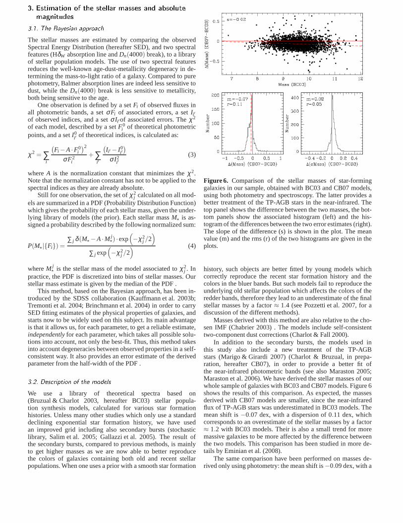
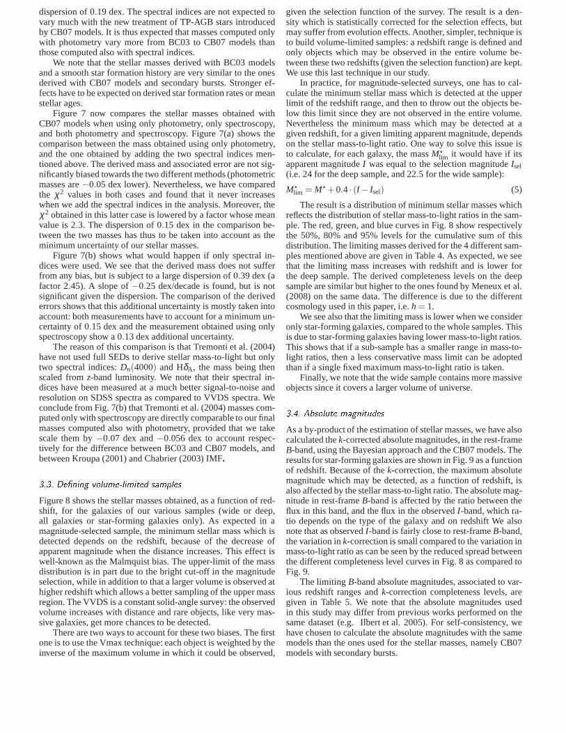
Figure 6. Comparison of the stellar masses of star-forminggalaxies in our sample, obtained with BC03 and CB07 models,using both photometry and spectroscopy. The latter provides abetter treatment of the TP-AGB stars in the near-infrared. Thetop panel shows the difference between the two masses, the bot-tom panels show the associated histogram (left) and the his-togram of the differences between the two error estimates (right).The slope of the difference (s) is shown in the plot. The meanvalue (m) and the rms (r) of the two histograms are given in theplots.

history, such objects are better fitted by young models whichcorrectly reproduce the recent star formation history and thecolors in the bluer bands. But such models fail to reproduce theunderlying old stellar population which affects the colorsof theredder bands, therefore they lead to an underestimate of thefinalstellar masses by a factor≈ 1.4 (see Pozzetti et al. 2007, for adiscussion of the different methods).

Masses derived with this method are also relative to the cho-sen IMF (Chabrier 2003) . The models include self-consistenttwo-component dust corrections (Charlot & Fall 2000).

In addition to the secondary bursts, the models used inthis study also include a new treatment of the TP-AGBstars (Marigo & Girardi 2007) (Charlot & Bruzual, in prepa-ration, hereafter CB07), in order to provide a better fit ofthe near-infrared photometric bands (see also Maraston 2005;Maraston et al. 2006). We have derived the stellar masses of ourwhole sample of galaxies with BC03 and CB07 models. Figure 6shows the results of this comparison. As expected, the massesderived with CB07 models are smaller, since the near-infraredflux of TP-AGB stars was underestimated in BC03 models. Themean shift is−0.07 dex, with a dispersion of 0.11 dex, whichcorresponds to an overestimate of the stellar masses by a factor≈ 1.2 with BC03 models. Their is also a small trend for moremassive galaxies to be more affected by the difference betweenthe two models. This comparison has been studied in more de-tails by Eminian et al. (2008).

The same comparison have been performed on masses de-rived only using photometry: the mean shift is−0.09 dex, with a

∼

dispersion of 0.19 dex. The spectral indices are not expected tovary much with the new treatment of TP-AGB stars introducedby CB07 models. It is thus expected that masses computed onlywith photometry vary more from BC03 to CB07 models thanthose computed also with spectral indices.

We note that the stellar masses derived with BC03 modelsand a smooth star formation history are very similar to the onesderived with CB07 models and secondary bursts. Stronger ef-fects have to be expected on derived star formation rates or meanstellar ages.

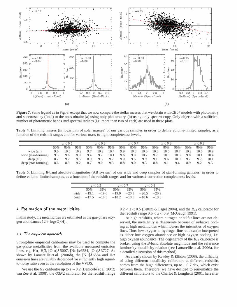
Figure 7 now compares the stellar masses obtained withCB07 models when using only photometry, only spectroscopy,and both photometry and spectroscopy. Figure 7(a) shows thecomparison between the mass obtained using only photometry,and the one obtained by adding the two spectral indices men-tioned above. The derived mass and associated error are not sig-nificantly biased towards the two different methods (photometricmasses are−0.05 dex lower). Nevertheless, we have comparedthe χ2 values in both cases and found that it never increaseswhen we add the spectral indices in the analysis. Moreover, theχ2 obtained in this latter case is lowered by a factor whose meanvalue is 2.3. The dispersion of 0.15 dex in the comparison be-tween the two masses has thus to be taken into account as theminimum uncertainty of our stellar masses.

Figure 7(b) shows what would happen if only spectral in-dices were used. We see that the derived mass does not sufferfrom any bias, but is subject to a large dispersion of 0.39 dex (afactor 2.45). A slope of−0.25 dex/decade is found, but is notsignificant given the dispersion. The comparison of the derivederrors shows that this additional uncertainty is mostly taken intoaccount: both measurements have to account for a minimum un-certainty of 0.15 dex and the measurement obtained using onlyspectroscopy show a 0.13 dex additional uncertainty.

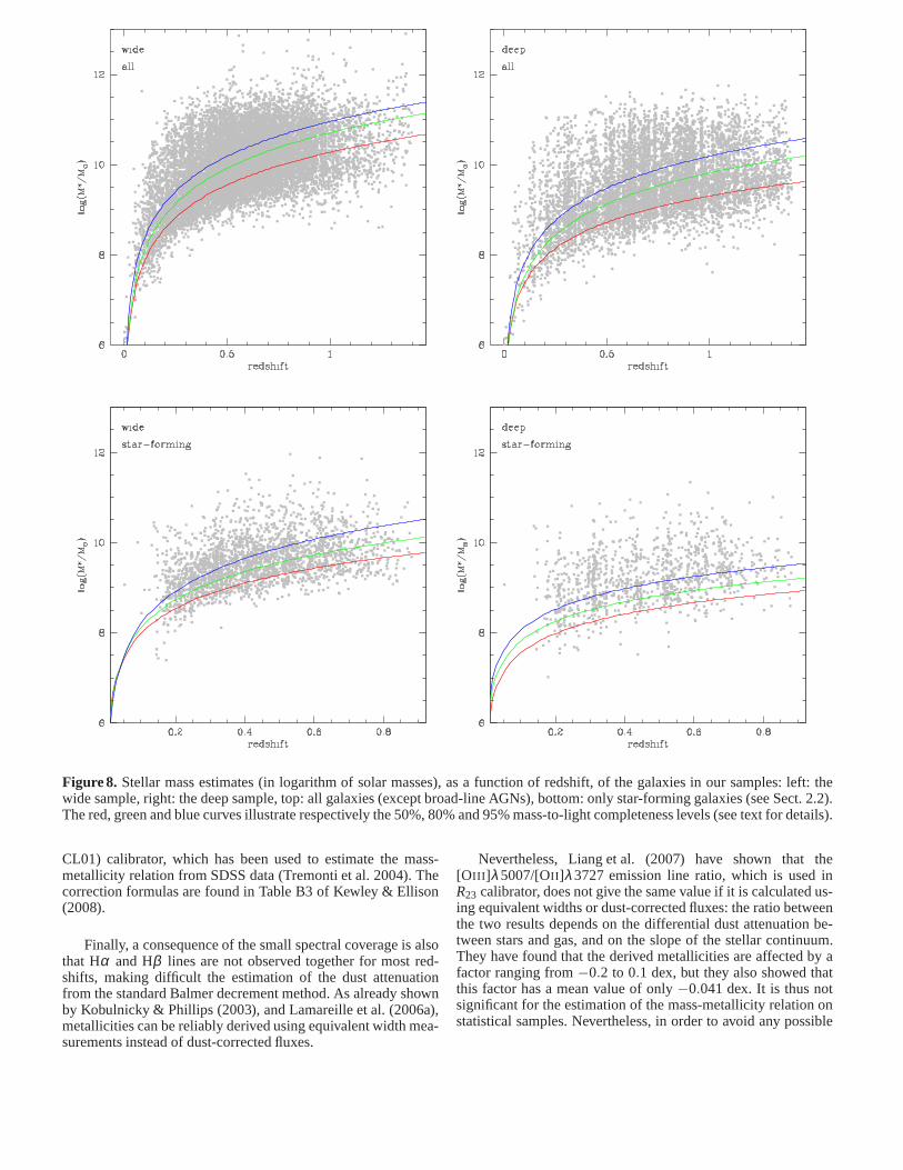
The reason of this comparison is that Tremonti et al. (2004)have not used full SEDs to derive stellar mass-to-light but onlytwo spectral indices:Dn(4000) and HδA , the mass being thenscaled fromz-band luminosity. We note that their spectral in-dices have been measured at a much better signal-to-noise andresolution on SDSS spectra as compared to VVDS spectra. Weconclude from Fig. 7(b) that Tremonti et al. (2004) masses com-puted only with spectroscopy are directly comparable to ourfinalmasses computed also with photometry, provided that we takescale them by−0.07 dex and−0.056 dex to account respec-tively for the difference between BC03 and CB07 models, andbetween Kroupa (2001) and Chabrier (2003) IMF.3.3. Dening volume-limited samplesFigure 8 shows the stellar masses obtained, as a function of red-shift, for the galaxies of our various samples (wide or deep,all galaxies or star-forming galaxies only). As expected inamagnitude-selected sample, the minimum stellar mass whichisdetected depends on the redshift, because of the decrease ofapparent magnitude when the distance increases. This effect iswell-known as the Malmquist bias. The upper-limit of the massdistribution is in part due to the bright cut-off in the magnitudeselection, while in addition to that a larger volume is observed athigher redshift which allows a better sampling of the upper massregion. The VVDS is a constant solid-angle survey: the observedvolume increases with distance and rare objects, like very mas-sive galaxies, get more chances to be detected.

There are two ways to account for these two biases. The firstone is to use the Vmax technique: each object is weighted by theinverse of the maximum volume in which it could be observed,

given the selection function of the survey. The result is a den-sity which is statistically corrected for the selection effects, butmay suffer from evolution effects. Another, simpler, technique isto build volume-limited samples: a redshift range is definedandonly objects which may be observed in the entire volume be-tween these two redshifts (given the selection function) are kept.We use this last technique in our study.

In practice, for magnitude-selected surveys, one has to cal-culate the minimum stellar mass which is detected at the upperlimit of the redshift range, and then to throw out the objectsbe-low this limit since they are not observed in the entire volume.Nevertheless the minimum mass which may be detected at agiven redshift, for a given limiting apparent magnitude, dependson the stellar mass-to-light ratio. One way to solve this issue isto calculate, for each galaxy, the massM⋆

lim it would have if itsapparent magnitudeI was equal to the selection magnitudeIsel(i.e. 24 for the deep sample, and 22.5 for the wide sample):

M⋆lim = M⋆ +0.4 · (I − Isel) (5)

The result is a distribution of minimum stellar masses whichreflects the distribution of stellar mass-to-light ratios in the sam-ple. The red, green, and blue curves in Fig. 8 show respectivelythe 50%, 80% and 95% levels for the cumulative sum of thisdistribution. The limiting masses derived for the 4 different sam-ples mentioned above are given in Table 4. As expected, we seethat the limiting mass increases with redshift and is lower forthe deep sample. The derived completeness levels on the deepsample are similar but higher to the ones found by Meneux et al.(2008) on the same data. The difference is due to the differentcosmology used in this paper, i.e.h = 1.

We see also that the limiting mass is lower when we consideronly star-forming galaxies, compared to the whole samples.Thisis due to star-forming galaxies having lower mass-to-lightratios.This shows that if a sub-sample has a smaller range in mass-to-light ratios, then a less conservative mass limit can be adoptedthan if a single fixed maximum mass-to-light ratio is taken.

Finally, we note that the wide sample contains more massiveobjects since it covers a larger volume of universe.3.4. Absolute magnitudesAs a by-product of the estimation of stellar masses, we have alsocalculated thek-corrected absolute magnitudes, in the rest-frameB-band, using the Bayesian approach and the CB07 models. Theresults for star-forming galaxies are shown in Fig. 9 as a functionof redshift. Because of thek-correction, the maximum absolutemagnitude which may be detected, as a function of redshift, isalso affected by the stellar mass-to-light ratio. The absolute mag-nitude in rest-frameB-band is affected by the ratio between theflux in this band, and the flux in the observedI -band, which ra-tio depends on the type of the galaxy and on redshift We alsonote that as observedI -band is fairly close to rest-frameB-band,the variation ink-correction is small compared to the variation inmass-to-light ratio as can be seen by the reduced spread betweenthe different completeness level curves in Fig. 8 as compared toFig. 9.

The limiting B-band absolute magnitudes, associated to var-ious redshift ranges andk-correction completeness levels, aregiven in Table 5. We note that the absolute magnitudes usedin this study may differ from previous works performed on thesame dataset (e.g. Ilbert et al. 2005). For self-consistency, wehave chosen to calculate the absolute magnitudes with the samemodels than the ones used for the stellar masses, namely CB07models with secondary bursts.

∼

(a) (b)

Figure 7.Same legend as in Fig. 6, except that we now compare the stellar masses that we obtain with CB07 models with photometryand spectroscopy (final) to the ones obtain: (a) using only photometry, (b) using only spectroscopy. Only objects with a sufficientnumber of photometric bandsandspectral indices (i.e. more than two of each) are used in these plots.

Table 4. Limiting masses (in logarithm of solar masses) of our various samples in order to define volume-limited samples, as afunction of the redshift ranges and for various mass-to-light completeness levels.

z< 0.5 z< 0.6 z< 0.7 z< 0.8 z< 0.950% 80% 95% 50% 80% 95% 50% 80% 95% 50% 80% 95% 50% 80% 95%

wide (all) 9.6 10.0 10.2 9.7 10.2 10.4 9.9 10.3 10.6 10.0 10.5 10.7 10.2 10.6 10.9wide (star-forming) 9.3 9.6 9.9 9.4 9.7 10.1 9.6 9.9 10.2 9.7 10.0 10.3 9.8 10.1 10.4

deep (all) 8.7 9.2 9.5 8.9 9.3 9.7 9.0 9.5 9.9 9.1 9.6 10.0 9.2 9.7 10.1deep (star-forming) 8.6 8.9 9.2 8.7 9.0 9.3 8.8 9.0 9.3 8.8 9.1 9.4 8.9 9.2 9.5

Table 5. Limiting B-band absolute magnitudes (AB system) of our wide and deep samples of star-forming galaxies, in order todefine volume-limited samples, as a function of the redshiftranges and for variousk-correction completeness levels.

z< 0.5 z< 0.7 z< 0.950% 95% 50% 95% 50% 95%

wide −19.1 −19.6 −19.9 −20.3 −20.5 −20.9deep −17.5 −18.3 −18.2 −18.9 −18.6 −19.34. Estimation of the metalli ities

In this study, the metallicities are estimated as the gas-phase oxy-gen abundances 12+ log(O/H).4.1. The empiri al approa hStrong-line empirical calibrators may be used to compute thegas-phase metallicities from the available measured emissionlines, e.g. Hα, Hβ , [OIII ]λ5007, [NII ]λ6584, [OII ]λ3727. Asshown by Lamareille et al. (2006b), the [NII ]λ6584 and Hαemission lines are reliably deblended for sufficiently highsignal-to-noise ratio even at the resolution of the VVDS.

We use theN2 calibrator up toz∼ 0.2 (Denicoló et al. 2002;van Zee et al. 1998), theO3N2 calibrator for the redshift range

0.2 < z< 0.5 (Pettini & Pagel 2004), and theR23 calibrator forthe redshift range 0.5 < z< 0.9 (McGaugh 1991).

At high redshifts, where nitrogen or sulfur lines are not ob-served, the metallicity is degenerate because of radiativecool-ing at high metallicities which lowers the intensities of oxygenlines. Thus, low oxygen-to-hydrogen line ratio can be interpretedas either low oxygen abundance or high oxygen cooling, i.e.high oxygen abundance. The degeneracy of theR23 calibrator isbroken using theB-band absolute magnitude and the referenceluminosity-metallicity relation (see Lamareille et al. 2006a, fora detailed discussion of this method).

As clearly shown by Kewley & Ellison (2008), the difficultyof using different metallicity calibrators at different redshiftscomes from the huge differences, up to±0.7 dex, which existbetween them. Therefore, we have decided to renormalize thedifferent calibrators to the Charlot & Longhetti (2001, hereafter

∼

Figure 8. Stellar mass estimates (in logarithm of solar masses), as a function of redshift, of the galaxies in our samples: left: thewide sample, right: the deep sample, top: all galaxies (except broad-line AGNs), bottom: only star-forming galaxies (see Sect. 2.2).The red, green and blue curves illustrate respectively the 50%, 80% and 95% mass-to-light completeness levels (see textfor details).

CL01) calibrator, which has been used to estimate the mass-metallicity relation from SDSS data (Tremonti et al. 2004).Thecorrection formulas are found in Table B3 of Kewley & Ellison(2008).

Finally, a consequence of the small spectral coverage is alsothat Hα and Hβ lines are not observed together for most red-shifts, making difficult the estimation of the dust attenuationfrom the standard Balmer decrement method. As already shownby Kobulnicky & Phillips (2003), and Lamareille et al. (2006a),metallicities can be reliably derived using equivalent width mea-surements instead of dust-corrected fluxes.

Nevertheless, Liang et al. (2007) have shown that the[OIII ]λ5007/[OII ]λ3727 emission line ratio, which is used inR23 calibrator, does not give the same value if it is calculated us-ing equivalent widths or dust-corrected fluxes: the ratio betweenthe two results depends on the differential dust attenuation be-tween stars and gas, and on the slope of the stellar continuum.They have found that the derived metallicities are affectedby afactor ranging from−0.2 to 0.1 dex, but they also showed thatthis factor has a mean value of only−0.041 dex. It is thus notsignificant for the estimation of the mass-metallicity relation onstatistical samples. Nevertheless, in order to avoid any possible

∼

Figure 9.Absolute magnitudes estimates in the rest-frameB-band (AB system), as a function of redshift, of the star-forming galaxiesof the wide (left) and deep (right) samples. The red, green and blue lines illustrate respectively the 50%, 80% and 95%k-correctioncompleteness levels (see text for details).

bias on a different sample, we decided to use their correctiveformula based on theDn(4000) index.4.2. The Bayesian approa hThe metallicities may also be estimated using again the Bayesianapproach. The relative fluxes of all measured emission linesare compared to a set of photoionization models, which pre-dicts the theoretical flux ratios given four parameters: thegas-phase metallicity, the ionization level, the dust-to-metal ra-tio and the reddening (Charlot & Longhetti 2001). The CL01models are based on population synthesis for the ionizingflux (Bruzual & Charlot 2003), emission line modeling (Cloudy,Ferland 2001) and a two-component dust attenuation law(Charlot & Fall 2000).

We calculate theχ2 of each model and summarize them inthe PDF of the metallicity using a similar method than describedabove in Eq. 3 and 4, but now applied to emission-line fluxes in-stead of photometric points. Only the emission lines with enoughsignal-to-noise (S/N>4) are used in the fit. This method is ap-plied directly on observed line fluxes: the correction for dust at-tenuation is included self-consistently in the models.

The O/H degeneracy at high redshift ends up with double-peaked PDFs: one peak for the low metallicity solution and an-other one at high metallicity. However, other information suchas dust extinction, ionization level, or star formation rate helpaffecting to the two peaks two different probabilities. Thus, wesolve the degeneracy by fitting two peaks in the PDFs, and bykeeping the one with the highest probability. As already dis-cussed in Lamareille et al. (2006a), this method cannot be usedto chose the metallicity of one single galaxy, but it can be usedstatistically to derive a mean metallicity, e.g. as a function ofmass.

In this study, given the relatively low spectral resolutionandspectral coverage of our spectra, we use the CL01 method only

as a check of the quality of empirically-calibrated metallicities.The three main advantages of checking our results with the CL01method are:(i) the use of one unique calibrator for all redshiftranges;(ii) the different method to deal with dust extinction,i.e. the self-consistent correction instead of the use of equivalentwidths; (iii) the different method to break the O/H degeneracy,i.e. the fit of the double-peaked PDF instead of the use of theluminosity.

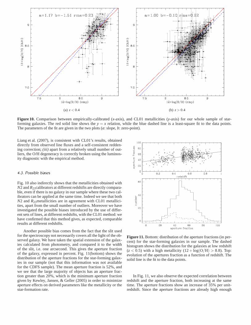
Fig. 10 shows the comparison between the empirically-calibrated and the CL01 metallicities. Apart from a small num-ber of outliers (7%), the two results are in good agreement withina dispersion of approximately 0.22 dex. This dispersion can becompared with the intrinsic dispersion of the mass-metallicityrelation, which is also of∼ 0.22 dex. We have also calculatedthe mean of the error bars for the two methods: 0.06 dex for theempirical method, and 0.18 dex for the CL01 method.

Let us summarize all the contributions to the global dis-persion.(i) The empirically-calibrated errors have been esti-mated from basic propagation of the line measurement errors.We know from tests performed on duplicated observations thatplatefit_vimoserrors are not underestimated. They reflect thenegligible contribution of noise to the global dispersion.(ii)Conversely, the CL01 errors have been estimated from the widthof the PDF. They also reflect the additional dispersion due tothedegeneracies in the models, which are taken into account thanksto the Bayesian approach.(iii) Finally the difference betweenthe mean CL01 error and the global dispersion reflects real vari-ations in the physical parameters of galaxies, which are nottakeninto account in both models.

The comparison between the two methods have shownthat: (i) the various empirical calibrators used at different red-shift ranges give consistent results with the CL01 metallicities,thanks to the correction formulas provided by Kewley & Ellison(2008); (ii) the empirical correction for dust attenuation us-ing equivalent widths, and the correction formula providedby

∼

(a) z< 0.4 (b) z> 0.4

Figure 10. Comparison between empirically-calibrated (x-axis), and CL01 metallicities (y-axis) for our whole sample of star-forming galaxies. The red solid line shows they = x relation, while the blue dashed line is a least-square fit to the data points.The parameters of the fit are given in the two plots (a: slope,b: zero-point).

Liang et al. (2007), is consistent with CL01’s results, obtaineddirectly from observed line fluxes and a self-consistent redden-ing correction;(iii) apart from a relatively small number of out-liers, the O/H degeneracy is correctly broken using the luminos-ity diagnostic with the empirical method.4.3. Possible biasesFig. 10 also indirectly shows that the metallicities obtained withN2 andR23calibrators at different redshifts are directly compara-ble, even if there is no galaxy in our sample where these two cal-ibrators can be applied at the same time. Indeed we see that bothN2 andR23metallicities are in agreement with CL01 metallici-ties, apart from the small number of outliers. Moreover we haveinvestigated the possible biases introduced by the use of differ-ent sets of lines, at different redshifts, with the CL01 method: wehave confirmed that this method gives, as expected, comparableresults at different redshifts.

Another possible bias comes from the fact that the slit usedfor the spectroscopy not necessarily covers all the light ofthe ob-served galaxy. We have taken the spatial extension of the galax-ies calculated from photometry, and compared it to the widthof the slit, i.e. one arcsecond. This gives the aperture fractionof the galaxy, expressed in percent. Fig. 11(bottom) shows thedistribution of the aperture fractions for the star-forming galax-ies in our sample (not that this information was not availablefor the CDFS sample). The mean aperture fraction is 52%, andwe see that the large majority of objects has an aperture frac-tion greater than 20%, which is the minimum aperture fractiongiven by Kewley, Jansen, & Geller (2005) in order to minimizeaperture effects on derived parameters like the metallicity or thestar-formation rate.

Figure 11.Bottom: distribution of the aperture fractions (in per-cent) for the star-forming galaxies in our sample. The dashedhistogram shows the distribution for the galaxies at low redshift(z < 0.5) with a high metallicity (12+ log(O/H) > 8.8). Top:evolution of the apertures fraction as a function of redshift. Thesolid line is the fit to the data points.

In Fig. 11, we also observe the expected correlation betweenredshift and the aperture fraction, both increasing at the sametime. The aperture fractions show an increase of 35% per unit-redshift. Since the aperture fractions are already high enough

∼

at low redshift not to affect the derived metallicities, andsincethey increase with redshift, this slope is likely to have a marginaleffect on the derived evolution of metallicity as a functionofredshift.5. The luminosity-metalli ity relation5.1. Study of the derived tsWe study in this section the relation between the rest-frameB-band luminosity and gas-phase metallicity, for the star-forminggalaxies of our wide and deep samples. Here we use the metal-licities estimated with the empirical approach, and renormal-ized to the CL01 method (see Sect. 4.1). Figure 12 shows theluminosity-metallicity relation of the wide and deep samples inthree redshift ranges: 0.0 < z< 0.5, 0.5< z< 0.7 and 0.7< z<0.9. The results are compared to the luminosity-metallicity rela-tion in the local universe derived by Lamareille et al. (2004) with2dFGRS data, and renormalized to the CL01 method. In order todo this comparison, we have done a linear fit to the data points.

As already shown before, the luminosity-metallicity relationis characterized by an non-negligible dispersion of the order of≈ 0.25 dex (higher than the one of the mass-metallicity relation).Therefore, the method used to perform the fit has a huge impacton the results, and it is mandatory to use the same method beforedoing comparisons between two studies. Thus, we have used thesame method than Lamareille et al. (2004), i.e. the ols bisectorfit (Isobe et al. 1990), starting from the 50%k-correction com-pleteness level (see Sect. 3.4). The results are shown in Fig. 12and in Table 6.

The slope is by∼ 2σ steeper than the one of the reference re-lation in the local universe, this slope being similar in allredshiftranges (≈ −0.75), except 0.5 < z< 0.7 in the deep sample. Asalready shown by Lamareille et al. (2004) who have comparedthe slopes of the luminosity-metallicity relation for low and highmetallicity objects, this slope is steeper for high metallicity ob-jects. This effect has been confirmed by Lee et al. (2006) whohave extended the mass-metallicity relation of Tremonti etal.(2004) to lower masses and metallicities and found a flatterslope. We emphasize that we are not discussing here the sat-uration at 12+ log(O/H) ≈ 9.2 as observed by Tremonti et al.(2004), and which might be confused with a flatter slope at veryhigh metallicity.

Thus, given that we expect a steeper slope at high metallicity,we analyze our results as a lack of data points in the low metal-licity region: the wide sample does not go deep enough to detectlow-metallicity and low-luminosity objects above the complete-ness limit. Moreover, in the 0.0< z< 0.5 redshift range of wideand deep samples, the S/N>4 cut on emission lines introducesa bias towards high metallicity objects: the faint and blended[N II ]λ6584 line, used to compute metallicities in this redshiftrange, becomes rapidly undetectable at low metallicities.

The apparently high number of galaxies with low redshift,low luminosity and high metallicity seen in Fig. 12(left) maybe explained by two effects. First, as said in previous paragraph,the [NII ]λ6584 line is more likely to be observed for high metal-licity objects. There is consequently a lack of objects withlowluminosity and low metallicity which makes the distribution ap-parently wrong (as compared to previous studies). Second, theseobjects at low redshift may have lower aperture fractions, whichmay introduce a bias towards higher metallicities given that wepreferentially observe their central part. Indeed, we haveplotthe distribution of the aperture fractions for objects witha low

redshift and a high metallicity in Fig. 11(bottom, dashed his-togram): they are clearly lower, with a mean of 40%.

We recognize that the results obtained by doing a direct lin-ear fit to data points suffer from a drawback: the correlationsbetween metallicity and luminosity shown in Fig. 12 are weak.This weakness is characterized by the non-negligible errorbarsfor the slopes and the zero-points of the relations providedinTable 6, and also by low Spearman correlation rank coefficients:of the order of−0.3 for the bottom-center panel, and−0.1 forthe other panels.5.2. Global metalli ity evolutionDespite the weakness of the correlations found in our data, weknow from previous studies that the luminosity-metallicity ex-ists. Thus we can use the existence of this relation as an assump-tion and find new results.

In order to quantify the evolution of the luminosity-relation,we can also derive the mean evolution of metallicity. This isdonewith the additional assumption that the slope of the luminosity-relation remains constant slope at zero-order. The resultsareshown in Fig. 12 and in Table 6. As expected, the evolutionis barely significant in the 0.0 < z < 0.5 redshift range. In the0.5 < z< 0.7 and 0.7 < z< 0.9 redshift ranges, the evolution isstronger. It is similar in the wide sample to what has been foundby Lamareille et al. (2006a). In the 0.5 < z< 0.7 redshift rangeof the deep sample, the results are similar with both methods,which confirms the hypothesis that a steeper slope is found onlywhen low-metallicity points are not included in the fit.

Finally, the comparison of the wide and deep samples showa stronger evolution of the metallicity with redshift in thewidesample. This result tells us that the slopedoes not actuallyremain constant, and that the evolution of the metallicity isstronger in more luminous objects. Atz∼ 0.76, galaxies with anabsoluteB-band magnitude of∼ −20.1 have−0.32 dex lowermetallicities than galaxies of similar luminosities in thelocaluniverse, while galaxies with an absoluteB-band magnitude of∼−21.2 have−0.65 dex lower metallicities.

We have checked that the results are stable when break-ing the O/H degeneracy at high redshift with a different refer-ence relation (e.g. lowered in metallicity). As stated before byLamareille et al. (2006a), the use of a lower reference relation tobreak the degeneracy only changes the metallicities of the galax-ies in the intermediate region (12+ log(O/H) ≈ 8.3), thus non-significantly changing the whole luminosity-metallicity relation.

We have also checked the effect of not including the candi-date star-forming galaxies in the fit. As stated in Sect. 2.2,thecontamination of candidate star-forming galaxies by AGNs isless than 1%, and is thus not expected to affect significantlytheluminosity-metallicity relation. Therefore, the resultsof not in-cluding the candidate star-forming galaxies are only givenas in-formation in Table 6. We have also checked the effect of includ-ing candidate AGNs. In both cases, the effect on the luminosity-metallicity relation is very small.

We need to disentangle between the two effects which makethese objects more luminous, i.e. a higher mass or a lower mass-to-light ratio, which one is responsible of the stronger evolutionof the metallicity. Thus, we now study the mass-metallicityrela-tion in the next section.

∼

Figure 12.Rest-frameB-band luminosity-metallicity relation for the wide (top) and deep (bottom) samples, for three redshift ranges:from left to right 0.0< z< 0.5, 0.5< z< 0.7 and 0.7< z< 0.9. The metallicities have been estimated using the empirical approach(see Sect. 4.1). The solid line shows the luminosity-metallicity relation at low redshift derived by Lamareille et al. (2004), andrenormalized to the CL01 method. The short-dashed line shows the fit to the data points using the ols bisector method (see text).The long-dashed lines shows the fit to the data points assuming a constant slope.

Table 6.Evolution of the luminosity-metallicity relation for the wide and deep samples. The reference relation is the one obtainedby Lamareille et al. (2004) with 2dFGRS data and renormalized to the CL01 method. In each redshift ranges, we give the results ofthe ols bisector fit (slope and zero-point) and of the constant-slope fit (mean shift, see Fig. 12), together with the mean redshift andmagnitude, and the dispersion of the relation. The metallicity shift is given in three cases:a) using only star-forming galaxies,b)adding candidate star-forming galaxies, andc) adding also candidate AGNs.

sample slope zero-point z MAB(B) ∆ log(O/H)L rmsa b c

reference −0.31 2.83wide0.0 < z< 0.5 −0.67±0.17 −4.60±3.4 0.31 −19.99 −0.08 −0.10 −0.10 0.230.5 < z< 0.7 −0.75±0.08 −6.67±1.6 0.59 −20.53 −0.39 −0.44 −0.45 0.230.7 < z< 0.9 −0.64±0.21 −5.01±4.4 0.77 −21.22 −0.58 −0.65 −0.70 0.24deep0.0 < z< 0.5 −0.90±0.45 −8.28±8.61 0.30 −18.99 0.17 0.15 0.15 0.280.5 < z< 0.7 −0.41±0.06 0.50±1.29 0.59 −19.67 −0.20 −0.24 −0.25 0.270.7 < z< 0.9 −0.87±0.41 −8.89±8.20 0.76 −20.05 −0.24 −0.32 −0.39 0.296. The mass-metalli ity relation6.1. Global metalli ity evolution

We now derive the mass-metallicity relation for the star-forminggalaxies of the wide and deep samples, using the empirical ap-proach for computing the metallicities, and in three redshiftranges: 0.0 < z< 0.5, 0.5 < z< 0.7 and 0.7 < z< 0.9. The re-sults are shown in Fig. 13 and Table 7, and are compared to thereference mass-metallicity relation in the local universe, derivedby Tremonti et al. (2004) with SDSS data. The reference relation

has been shifted in mass, in order to take into account the effectof using different models (see Sect. 3.2).

As in Fig. 12, the data points shown in Fig. 13 do not showstrong Spearman rank correlation coefficients. We thus skipthestep of doing a fit to these data points. We directly probe theglobal evolution in metallicity of star-forming galaxies com-pared to the reference relation, doing the likely assumption thatthe mass-metallicity relation exists also at high redshift. To doso, we calculate the mean shift in metallicity by fitting to thedata points the same curve than Eq. 3 of Tremonti et al. (2004),allowing only a different zero-point. The zero-order assumptionis indeed that the shape of the mass-metallicity relation does

∼

Figure 13. The mass-metallicity relation of star-forming galaxies for the wide (top) and deep (bottom) samples, for three redshiftranges: from left to right 0.0 < z< 0.5, 0.5 < z< 0.7 and 0.7 < z< 0.9. The metallicities have been estimated using the empiricalapproach (see Sect. 4.1). The solid curve shows the mass-metallicity relation at low redshift derived by Tremonti et al.(2004). Thelong-dashed curves shows the fit to the data points assuming that the SDSS curve is only shifted down in metallicity.

Table 7. Evolution of the mass-metallicity relation for the wideand deep samples. The reference relation is the one obtainedbyTremonti et al. (2004) with SDSS data and the CL01 method,renormalized in mass. In each redshift ranges, we give the meanredshift, stellar mass, and metallicity shift (assuming that theshape of the relation remains constant, see Fig. 13), and thedis-persion of the relation. The metallicity shift is given in threecases:a) using only star-forming galaxies,b) adding candidatestar-forming galaxies, andc) adding also candidate AGNs.

sample z lg(M⋆) ∆ log(O/H)M rmsa b c

wide0.0 < z< 0.5 0.30 9.87 −0.08 −0.08 −0.09 0.170.5 < z< 0.7 0.59 9.97 −0.22 −0.25 −0.26 0.200.7 < z< 0.9 0.78 10.19 −0.23 −0.28 −0.36 0.19deep0.0 < z< 0.5 0.29 9.45 −0.04 −0.05 −0.05 0.200.5 < z< 0.7 0.59 9.45 −0.17 −0.21 −0.23 0.190.7 < z< 0.9 0.76 9.40 −0.12 −0.18 −0.23 0.20

not vary with redshift. The results are shown in Fig. 13 and inTable 7. The fit is performed above the 50% mass-to-light com-pleteness level.

There are some caveats in the interpretation of the massand metallicity evolution of the deep sample, because of selec-tion and statistical effects. The mean observed stellar seams todecrease with redshift, which is in contradiction of what onewould expect from the Malmquist bias. First, we find higherstellar masses than expected in the lowest redshift bin. Thesam-

ple is actually not complete down to the limiting mass: lowermass galaxies would have lower metallicities, and low metallic-ities are indeed difficult to measure because of the blendingof[N II ]λ6584 and Hα lines. Conversely, the highest redshift binhas a lower mean mass than expected, which is more probablydue to a statistical effect because of the small solid angle of thedeep sample. This later effect also explains why the metallicityevolution seems smaller in the highest redshift bin.

As observed on the luminosity-metallicity relation in previ-ous section, we clearly see a stronger metallicity evolution inthe wide sample than in the deep sample. The wide and deepsamples span interestingly different ranges in masses, butareotherwise identical. This effect thus shows that the most mas-sive galaxies have experienced the most significant evolutionin metallicity. At z∼ 0.77, galaxies at 109.4 solar masses have−0.18 dex lower metallicities than galaxies of similar massesin the local universe, while galaxies at 1010.2 solar masses have−0.28 dex lower metallicities. We therefore conclude that theshape of the mass-metallicity relation varies with redshift, so thatit was flatter in an earlier universe.

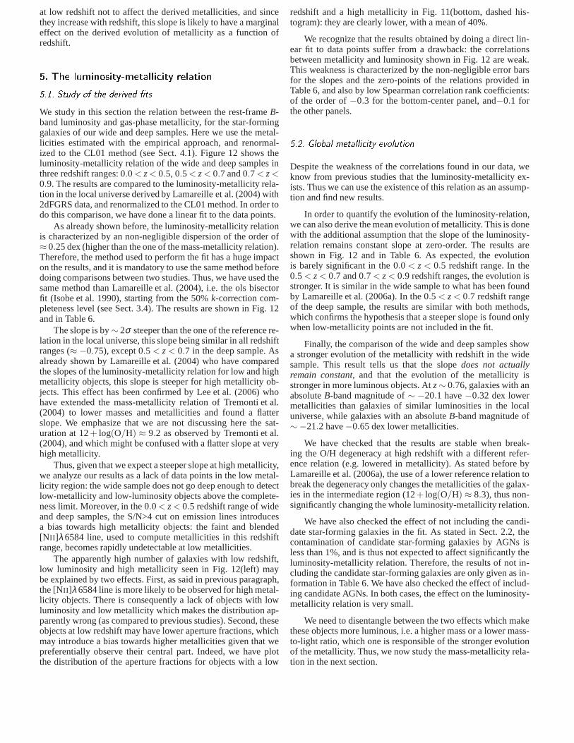
We also remark that like for the luminosity-metallicity re-lation, the potential influence of candidate AGNs or candidatestar-forming galaxies is negligible (see Table 7).6.2. Evolution of the shape of the mass-metalli ity relationWe now evaluate the evolution of the shape of the mass-metallicity relation as a function of redshift, by co-adding a num-ber of data points together in bins of mass, thus increasing thesignal-to-noise ratio. Figure 14 shows the results in threered-

∼

Figure 14. The mass-metallicity relation of star-forming galaxies for three redshift ranges: from left to right 0.2 < z< 0.5, 0.5 <z< 0.6 and 0.6< z< 0.8. The metallicities have been estimated using the empirical approach (see Sect. 4.1). The solid curve showsthe mass-metallicity relation at low redshift derived by Tremonti et al. (2004). We show the mean metallicities by bins of stellarmasses. The blue error bars represent the uncertainty on themean, while the green error bars represent the dispersion ofthe datapoints. The 50% mass-to-light completeness levels for the deep and wide samples (see Table 4) are shown as vertical dotted lines.

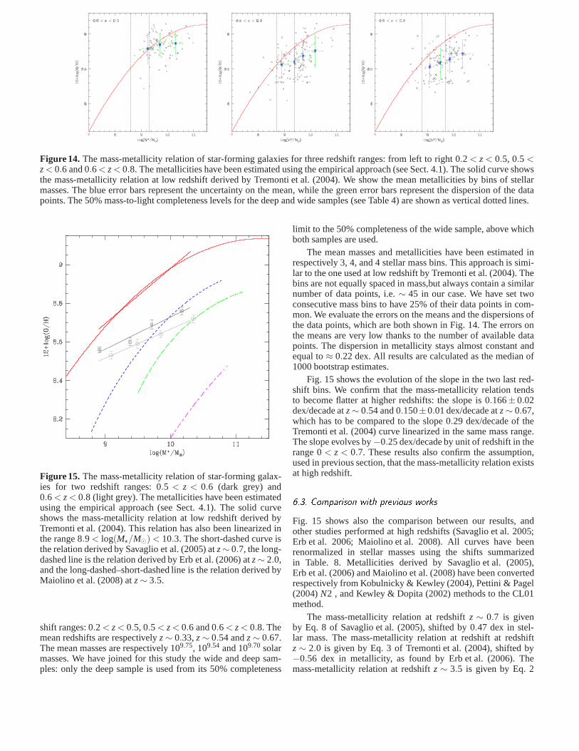
Figure 15. The mass-metallicity relation of star-forming galax-ies for two redshift ranges: 0.5 < z < 0.6 (dark grey) and0.6 < z< 0.8 (light grey). The metallicities have been estimatedusing the empirical approach (see Sect. 4.1). The solid curveshows the mass-metallicity relation at low redshift derived byTremonti et al. (2004). This relation has also been linearized inthe range 8.9 < log(M⋆/M⊙) < 10.3. The short-dashed curve isthe relation derived by Savaglio et al. (2005) atz∼ 0.7, the long-dashed line is the relation derived by Erb et al. (2006) atz∼ 2.0,and the long-dashed–short-dashed line is the relation derived byMaiolino et al. (2008) atz∼ 3.5.

shift ranges: 0.2 < z< 0.5, 0.5 < z< 0.6 and 0.6 < z< 0.8. Themean redshifts are respectivelyz∼ 0.33,z∼ 0.54 andz∼ 0.67.The mean masses are respectively 109.75, 109.54 and 109.70 solarmasses. We have joined for this study the wide and deep sam-ples: only the deep sample is used from its 50% completeness

limit to the 50% completeness of the wide sample, above whichboth samples are used.

The mean masses and metallicities have been estimated inrespectively 3, 4, and 4 stellar mass bins. This approach is simi-lar to the one used at low redshift by Tremonti et al. (2004). Thebins are not equally spaced in mass,but always contain a similarnumber of data points, i.e.∼ 45 in our case. We have set twoconsecutive mass bins to have 25% of their data points in com-mon. We evaluate the errors on the means and the dispersions ofthe data points, which are both shown in Fig. 14. The errors onthe means are very low thanks to the number of available datapoints. The dispersion in metallicity stays almost constant andequal to≈ 0.22 dex. All results are calculated as the median of1000 bootstrap estimates.

Fig. 15 shows the evolution of the slope in the two last red-shift bins. We confirm that the mass-metallicity relation tendsto become flatter at higher redshifts: the slope is 0.166± 0.02dex/decade atz∼ 0.54 and 0.150±0.01 dex/decade atz∼ 0.67,which has to be compared to the slope 0.29 dex/decade of theTremonti et al. (2004) curve linearized in the same mass range.The slope evolves by−0.25 dex/decade by unit of redshift in therange 0< z < 0.7. These results also confirm the assumption,used in previous section, that the mass-metallicity relation existsat high redshift.6.3. Comparison with previous worksFig. 15 shows also the comparison between our results, andother studies performed at high redshifts (Savaglio et al. 2005;Erb et al. 2006; Maiolino et al. 2008). All curves have beenrenormalized in stellar masses using the shifts summarizedin Table. 8. Metallicities derived by Savaglio et al. (2005),Erb et al. (2006) and Maiolino et al. (2008) have been convertedrespectively from Kobulnicky & Kewley (2004), Pettini & Pagel(2004)N2 , and Kewley & Dopita (2002) methods to the CL01method.

The mass-metallicity relation at redshiftz ∼ 0.7 is givenby Eq. 8 of Savaglio et al. (2005), shifted by 0.47 dex in stel-lar mass. The mass-metallicity relation at redshift at redshiftz∼ 2.0 is given by Eq. 3 of Tremonti et al. (2004), shifted by−0.56 dex in metallicity, as found by Erb et al. (2006). Themass-metallicity relation at redshiftz∼ 3.5 is given by Eq. 2

∼

Table 8. Different setups for different mass-metallicity relations found in the literature, and associated shifts to be applied to theirstellar masses in order for them to be comparable with our results. This table shows the type of data, the models, the presence or notof secondary bursts, and the IMF used to compute the stellar masses. The last column gives the global shift that has to be applied tothe logarithm of the stellar mass.

References† data⋆ model bursts IMF† sumour study P+S CB07 yes C03T04 S BC03 yes K01

+0.00 −0.07 - −0.056 −0.126S05 P Pégase yes BG03

+0.05 −0.09 - +0.024 −0.016E06 P BC03 no C03

+0.05 −0.09 +0.14 - +0.1M08 P BC03 no S55

+0.05 −0.09 +0.14 −0.232 −0.132

⋆S stands for spectroscopy, P stands for photometry.†T04: Tremonti et al. (2004); S05: Savaglio et al. (2005); E06: Erb et al. (2006); M08: Maiolino et al. (2008); C03: Chabrier (2003); K01: Kroupa(2001); BG03: Baldry & Glazebrook (2003); S55: Salpeter (1955).

of Maiolino et al. (2008), with the parameters given in theirTable 5.

Contrary to Savaglio et al. (2005), we find a flatter slope ofthe mass-metallicity relation atz∼ 1. Nevertheless, the compar-ison of data points shows that their results and ours are in goodagreement for the highest mass bins. The larger difference comesfrom the lowest mass bins, in which they are probably not com-plete. We know indeed that lower mass-to-light ratio galaxies arepreferentially observed in the lowest incomplete mass bins, andthat such galaxies show smaller mean metallicities (Ellison et al.2008).

The comparison with the data of Erb et al. (2006), whichare taken atz∼ 2, is less straightforward: there is a fairly goodagreement in metallicity with our high-mass end data, but actu-ally at a rather different redshift. This could mean that there havebeen very little metallicity evolution fromz∼ 2 to z∼ 1, butthis would be hard to understand when looking also at the otherresults. The metallicity evolves indeed strongly fromz ∼ 3.5(Maiolino et al. 2008), and betweenz∼ 1 and the local universe(our data and Savaglio et al. 2005). Nevertheless we note thatthis later discrepancy with Erb et al. (2006) results may be un-derstood: according to the downsizing scenario, the evolution ofthe most massive galaxies plotted here should be actually smallerbetweenz= 2 andz= 1 than betweenz= 1 andz= 0. Amongothers, Pérez-González et al. (2008) have quantified that galax-ies below log(M⋆/M⊙) = 11.5 have formed half of their stars atz< 1. The main reason of a possible overestimate of Erb et al.(2006) metallicities is probably statistical variation effects. Theyhave indeed based their results on stacked spectra of very fewgalaxies. The effect of the selection function is thereforediffi-cult to analyze.

The type of galaxies observed by Erb et al. (2006) atz∼ 2,which are active galaxies, may also have later evolved to “redand dead” passive galaxies, and got higher metallicities thanthe ones actually observed by us or by Tremonti et al. (2004)at lower redshifts. Such dead galaxies would unfortunatelynotsatisfy any more the selection function of any work based onemission-line measurements, and would not be observed.6.4. Evolution of the mass-to-light ratioThe metallicity evolution on the wide sample is very similarto what has been found by Lamareille et al. (2006a) on theluminosity-metallicity relation, after having applied a correction

Z Z

M

M

M(B)

M(B)

Figure 16. This plot shows, for galaxies with similar stellarmasses, their evolution when redshift increases: for metallicityin the mass-metallicity plane (top-left), for metallicityin theluminosity-metallicity plane (top-right), and for luminosity inthe mass-luminosity plane (bottom-right).

Table 9. Evolution of the mass-to-light ratio for the wide anddeep samples. This evolution is computed as an absolute rest-frameB-band magnitude evolution at constant stellar mass, fromthe comparison of the luminosity-metallicity (see Fig. 12 andTable 6) and mass-metallicity (see Fig. 13 and Table 7) relations.

∆MAB(B)redshift range wide deep0.0 < z< 0.5 −0.06 0.650.5 < z< 0.7 −0.61 −0.100.7 < z< 0.9 −1.19 −0.45

for luminosity evolution (Ilbert et al. 2005). This tells usthat thestronger evolution of the luminosity-metallicity relation, com-pared to the mass-metallicity relation, is effectively dueto anadditional luminosity evolution. This luminosity evolution hasto be understood for galaxies with similar masses, which means

∼

we can measure the evolution of the mass-to-light ratio in galax-ies using metallicity as a pivot.

Fig. 16 shows schematically the global evolution of metal-licity in the luminosity-metallicity plane (top-right). When thereis both an evolution of the metallicity in the mass-metallicityplane (top-left), and an evolution of the luminosity in the mass-luminosity plane (bottom-right), galaxies being more luminousat a given mass, the result is a stronger evolution of the metallic-ity in the luminosity-metallicity plane.

The luminosity evolution at constant mass of our galaxiescan be calculated using the following formula:

∆MAB(B) = a−1×(

∆ log(O/H)M −∆ log(O/H)L) (6)

wherea is the slope of the luminosity-metallicity relation, i.e.−0.31 dex/mag. The results are given in Table 9. The positiveevolution for the lowest redshift bin in the deep sample is dueto the incompleteness of theN2 calibration: at a given metallic-ity, our sample is biased towards higher luminosity. In the otherredshift ranges and the whole wide sample, we see that galax-ies at higher redshifts have lower mass-to-light ratios than today,and that this evolution is more significant for massive galaxies(i.e. the wide sample compared to the deep). These two resultsare in good agreement with the general scenario of downsizing(Cowie et al. 1996) for the evolution of the star formation rates ingalaxies. Less massive galaxies show a smaller evolution intheirstar formation rate atz< 1 since they are still actively formingstars.

It will be further analyzed in a subsequent paper of this se-ries.6.5. Derived star formation ratesWe now discuss the evolution of metallicity at constant stellarmass, in terms of star formation rates.

Assuming constant star formation rates (SFR) and theclosed-box model, one can calculate a stellar mass evolution andrelates it to a metallicity evolution using the following equations:

M⋆(t) = M⋆(0)+SFR× t (7)

M⋆(t)+Mg(t) = Mtot (8)

Z(t) = y× ln

(

1+M⋆(t)Mg(t)

)

(9)

whereM⋆, Mg andMtot are respectively the stellar mass, the gasmass, and the total baryonic mass of the galaxy (which remainconstant in the closed-box model); and whereZ andy are respec-tively the metallicity and the true yield (which depends only onthe stellar initial mass function).

We know the mass-metallicity relation at redshiftz = 0(Tremonti et al. 2004), and the Table 7 gives the metallicityevo-lution for various stellar masses and redshifts. Thus, we can re-vert Eq. 7, 8 and 9 to derive the star formation rate which ex-plains the observed values. The results are quoted in Table 10(casea). They are calculated for a given cosmology, and for atrue yieldy = 0.0104 (Tremonti et al. 2004).

A better modeling can be performed by taking into accountthe time evolution of the star formation rates in galaxies. Wemay for example assume an exponentially decreasing star for-mation rate, i.e.SFR(t) = SFR(0)×exp(−t/τ), whereτ givesthe characteristice-folding time of the galaxy. The exponentiallydecreasing law is a good choice when analyzing a population of

galaxies, with respect to the global cosmic evolution of star for-mation rate. Eq. 7 is then replaced by the following formula:

M⋆(t) = M⋆(0)+SFR(0)× τ ×(

1−e−t/τ)

(10)

Table 10 (caseb) gives the results obtained when assumingthe relation given by Eq. 12 of Savaglio et al. (2005) betweenthe e-folding time and the total baryonic mass of the galaxy.Comparing casesa and b, we see that the results are not dra-matically affected by the assumption of a decreasing SFR. Thestar formations activities in caseb are systematically higher thanin casea, which is expected as with a decreasing SFR a higherinitial value is needed to explain the same metallicity evolution,as compared to a constant SFR.

We note also that the derived star formation activities in thewide and deep samples are very close, despite their differentranges in stellar masses. In casea, star formation activities inthe deep sample are nevertheless higher than in the wide sam-ple, which is expected as the wide sample spans higher stellarmasses. Conversely, in caseb, we find higher star formationactivities for more massive objects. This comes from the as-sumption, made by Savaglio et al. (2005) and used in our equa-tions, that less massive galaxies have a longere-folding times.Consequently the less massive galaxies of the deep sample,which are assigned longe-folding times ans thus can be approx-imated as constant SFR, do not vary much from casea to casebwhile the more massive galaxies of the wide sample, which areassigned shorte-folding times, are more affected by the decreas-ing SFR hypothesis.

Preliminary results on the evolution of star formation activi-ties of VVDS galaxies, which will be presented in a subsequentpaper(see also Walcher et al. 2008), give at redshiftz≈ 0.6(our best sampled redshift bin) the following numbers:≈ 10−9.8

yr−1 for galaxies at≈ 109.5 solar masses (mean mass of the deepsample), and≈ 10−10.3 yr−1 for galaxies at≈ 1010 solar masses(mean mass the wide sample).

Assuming the closed-box hypothesis, our results in the widesample are in fairly good agreement with the observed star for-mation activities at similar masses, this agreement being betterin caseb. But in the deep sample, the inferred star formation ac-tivities which explain our observed metallicity evolutionseemsignificantly underestimated by a factor≈ 5. Although the vary-ing e-folding times hypothesis is in agreement with the slowerevolution of the mass-to-light ratio found in the deep sample inprevious section, it fails in providing a good agreement betweenour inferred star formation activities in the deep sample and ob-served values at similar masses. Moreover this hypothesis makemore massive galaxies forming stars more actively, which isincontradiction with observations.

We therefore conclude that the closed-box hypothesis is notvalid to explain our observed metallicity evolutions (assumingthat the preliminary results mentioned above are confirmed).7. Con lusionWe have calculated rest-frame luminosities, stellar massesand gas-phase oxygen abundances of a statistically significantsample of star-forming galaxies, selected from the VIMOSVLT Deep Survey. This has allowed us to derive luminosity-metallicity and mass-metallicity relations in various redshiftranges up toz∼ 0.9. These relations have also been derived intwo sub-samples: the deep sample which extends to lower ob-served luminosities thanks to a deeper magnitude selection, andthe wide sample which extends to higher luminosities thanksto

∼

Table 10. Derived star formation activities needed to explain the observed values quoted in Table 7, assuming the closed-boxmodel, andh = 0.7, Ωm = 0.3 andΩΛ = 0.7 cosmology. The values are given in the wide and deep samples, and for two differentassumptions:a) constant star formation rate,b) exponentially declining star formation rate (see text). Incaseb, each value is theinstantaneous star formation rate at the specified redshift(see Eq. 10).

mean redshift log(SFR/M⋆)wide deep

a b a b0.3 −11.06±0.7 −10.93±0.7 −11.05±0.9 −10.99±0.90.6 −10.64±0.5 −10.36±0.5 −10.51±0.4 −10.40±0.50.77 −10.73±0.4 −10.27±0.5 −10.65±0.5 −10.53±0.5

a larger solid angle. The selection function have been takenintoaccount in order to define volume- and mass-limited samples.

For both the wide and the deep samples, we have studiedas a function of redshift: the evolution in metallicity at constantluminosity, the evolution in metallicity at constant stellar mass,the associated evolution in luminosity at constant stellarmass,and the evolution of the slope of the mass-metallicity relation.

Additionally, we have also:

– Measured the fraction of star-forming galaxies and AGNs asa function of redshift.

– Calculated the difference in terms of stellar masses betweenthe old BC03 and new CB07 stellar population models.

– Studied the effect on the computation of stellar mass of theuse of spectral indices rather than only photometric points.

– Checked that gas-phase oxygen abundance measurements inlow and high redshift ranges are comparable even if calcu-lated with different methods.

– Studied the marginal effect of candidate star-forminggalaxies and candidate AGNs on the derived luminosity-metallicity or mass-metallicity relations.

In the wide sample, the mean evolution of metallicity at con-stant luminosity, and of luminosity at constant stellar mass, arein good agreement with previous studies by e.g. Lamareille et al.(2006a); Ilbert et al. (2005); Hammer et al. (2005) among oth-ers.

By doing the assumption that the slope of the luminosity-metallicity relation, or the shape of the mass-metallicityrela-tion, remain constant with redshift, we finally found differentmetallicity evolutions for the wide and deep samples. The wideand deep samples span different ranges in masses, which showsthat the assumption is wrong and that this slope or shape actu-ally evolves with redshift. We have found that the most massivegalaxies show the strongest metallicity evolution. Atz∼ 0.77,galaxies at 109.4 solar masses have−0.18 dex lower metallici-ties than galaxies of similar masses in the local universe, whilegalaxies at 1010.2 solar masses have−0.28 dex lower metallici-ties.

We have then studied the mass-metallicity relation on co-added data points by bins of stellar masses. The inferred slopesshow an evolution to a flatter mass-metallicity relation atz∼ 1 ascompared to the local universe, which confirms that higher massgalaxies show a stronger metallicity evolution during thisperiod.The slope evolves by−0.25 dex/decade by unit of redshift in therange 0< z< 0.7.

Moreover, we have inferred from our observations the starformation activities which explain this evolution in metallicity.To do so, we have assumed the closed-box hypothesis. We havefound that the observed metallicity evolution would be explainedby similar star formation activities at any mass, which is incon-tradiction with the well-known correlation between stellar mass

and star formation activity. Assuming preliminary observationsof the star formation activities in VVDS galaxies, we concludethat our results are underestimated by a factor≈ 5 in the deepsample, while their are in fair agreement in the wide sample.

These results make a strong evidence against the closed-box model. Indeed, we know from previous studies that the starformation activity of galaxies decreases while stellar mass in-creases. The only way to explain the smaller metallicity evolu-tion of the less massive galaxies is thus to replace in Eq. 9 thetrue yield by a smaller effective yield. Assuming a smaller effec-tive yield allows galaxies to show smaller metallicity evolution,even with a stronger star formation activity.

The smaller effective yield of less massive galaxies can beunderstood in the “open-closed” model. In this model, galax-ies with small stellar masses evolve like open-boxes: most ofthe metals produced during star formation are ejected in thein-tergalactic medium by stellar winds and supernovae feedback,the effective yield is thus very small. Conversely, galaxies withhigh stellar masses evolve in the open-closed model like closed-boxes: the metals are retained in the galaxy thanks to a highgravitational potential, the effective yield is thus closeto the trueyield.

The dependence of the effective yield with the gravitationalpotential of the galaxies, itself related to their total baryonicmass, has been already shown by Tremonti et al. (2004). It is nat-urally explained in the hierarchical galaxy formation scenario: incontrary to the closed-box model, the total baryonic mass doesnot remain constant and increases with time, together with thestellar mass, thanks to galaxy merging and accretion. This rela-tion between the stellar mass and the total baryonic mass is at theorigin of the mass-metallicity relation in the open-closedmodel,and is clearly supported by our data.

In the open-closed model, the smaller metallicity evolutionof less massive is naturally explained despite their stronger starformation activities.

We emphasize that Eq. 7, 8 and 10 are not valid any morein the open-closed model. It is not enough to replace, in Eq. 9,the true yield by the effective yield in order to infer the rightstar formation rates which explain the observed metallicity evo-lution. These equations must be modified to take also the dif-ference between the true and the effective yield into account.The way to modify these equations depends on the model usedto explain smaller effective yields (e.g. gas loss). Replacementequations can be found in other studies (e.g. Erb et al. 2006;Erb2008; Dalcanton 2007; Finlator & Davé 2008). We also refer thereader to subsequent papers of this series, for a more detaileddiscussion of the relation between the present results and theevolution of the star formation rates of galaxies, and for compar-isons with simulations (e.g. De Lucia et al. 2004).

Acknowledgements.We thank C. Tremonti for having made the originalplatefitcode available to the VVDS collaboration. F. Lamareille thanks the Osservatorio

∼

di Bologna for the receipt of a post-doctoral fellowship.This work has been partially supported by the CNRS-INSU and itsProgramme Nationaux de Galaxies et de Cosmologie (France),and byItalian Ministry (MIUR) grants COFIN2000 (MM02037133) andCOFIN2003(num.2003020150) and by INAF grants (PRIN-INAF 2005).The VLT-VIMOS observations have been carried out on guaranteed time (GTO)allocated by the European Southern Observatory (ESO) to theVIRMOS con-sortium, under a contractual agreement between the Centre National de laRecherche Scientifique of France, heading a consortium of French and Italianinstitutes, and ESO, to design, manufacture and test the VIMOS instrument.This work is based in part on data products produced at TERAPIX andthe Canadian Astronomy Data Centre as part of the Canada-France-HawaiiTelescope Legacy Survey, a collaborative project of NRC andCNRS.Referen esArnouts, S., Vandame, B., Benoist, C., et al. 2001, A&A, 379,740Baldry, I. K. & Glazebrook, K. 2003, ApJ, 593, 258Baldwin, J. A., Phillips, M. M., & Terlevich, R. 1981, PASP, 93, 5Brinchmann, J., Charlot, S., White, S. D. M., et al. 2004, MNRAS, 351, 1151Brodie, J. P. & Huchra, J. P. 1991, ApJ, 379, 157Brooks, A. M., Governato, F., Booth, C. M., et al. 2007, ApJ, 655, L17Bruzual, G. & Charlot, S. 2003, MNRAS, 344, 1000Chabrier, G. 2003, PASP, 115, 763Charlot, S. & Fall, S. M. 2000, ApJ, 539, 718Charlot, S. & Longhetti, M. 2001, MNRAS, 323, 887Cowie, L. L., Songaila, A., Hu, E. M., & Cohen, J. G. 1996, AJ, 112, 839Dalcanton, J. J. 2007, ApJ, 658, 941Davé, R. & Oppenheimer, B. D. 2007, MNRAS, 374, 427De Lucia, G., Kauffmann, G., & White, S. D. M. 2004, MNRAS, 349, 1101de Rossi, M. E., Tissera, P. B., & Scannapieco, C. 2007, MNRAS, 374, 323Denicoló, G., Terlevich, R., & Terlevich, E. 2002, MNRAS, 330, 69Ellison, S. L., Patton, D. R., Simard, L., & McConnachie, A. W. 2008, ApJ, 672,

L107Eminian, C., Kauffmann, G., Charlot, S., et al. 2008, MNRAS,384, 930Erb, D. K. 2008, ApJ, 674, 151Erb, D. K., Shapley, A. E., Pettini, M., et al. 2006, ApJ, 644,813Ferland, G. J. 2001, PASP, 113, 41Finlator, K. & Davé, R. 2008, MNRAS, 385, 2181Gallazzi, A., Charlot, S., Brinchmann, J., White, S. D. M., &Tremonti, C. A.

2005, MNRAS, 362, 41Garilli, B., Le Fèvre, O., Guzzo, L., et al. 2008, A&A, 804, accepted (astro-

ph/08044568)Garnett, D. R., Shields, G. A., Skillman, E. D., Sagan, S. P.,& Dufour, R. J.

1997, ApJ, 489, 63Gavignaud, I., Bongiorno, A., Paltani, S., et al. 2006, A&A,457, 79Giavalisco, M., Ferguson, H. C., Koekemoer, A. M., et al. 2004, ApJ, 600, L93Hammer, F., Flores, H., Elbaz, D., et al. 2005, A&A, 430, 115Ilbert, O., Tresse, L., Zucca, E., et al. 2005, A&A, 439, 863Iovino, A., McCracken, H. J., Garilli, B., et al. 2005, A&A, 442, 423Isobe, T., Feigelson, E. D., Akritas, M. G., & Babu, G. J. 1990, ApJ, 364, 104Kauffmann, G., Heckman, T. M., Tremonti, C., et al. 2003a, MNRAS, 346, 1055Kauffmann, G., Heckman, T. M., White, S. D. M., et al. 2003b, MNRAS, 341,

33Kewley, L. J. & Dopita, M. A. 2002, ApJS, 142, 35Kewley, L. J. & Ellison, S. L. 2008, AJ, 801, accepted (astro-ph/08011849)Kewley, L. J., Heisler, C. A., Dopita, M. A., & Lumsden, S. 2001, ApJS, 132,

37Kewley, L. J., Jansen, R. A., & Geller, M. J. 2005, PASP, 117, 227Kobulnicky, H. A. & Kewley, L. J. 2004, ApJ, 617, 240Kobulnicky, H. A. & Phillips, A. C. 2003, ApJ, 599, 1031Kobulnicky, H. A., Willmer, C. N. A., Phillips, A. C., et al. 2003, ApJ, 599, 1006Köppen, J., Weidner, C., & Kroupa, P. 2007, MNRAS, 375, 673Kroupa, P. 2001, MNRAS, 322, 231Lamareille, F. 2006, Ph.D. Thesis, http://tel.archives-ouvertes.fr/tel-

00090655/fr/Lamareille, F., Contini, T., Brinchmann, J., et al. 2006a, A&A, 448, 907Lamareille, F., Contini, T., Le Borgne, J.-F., et al. 2006b,A&A, 448, 893Lamareille, F., Mouhcine, M., Contini, T., Lewis, I., & Maddox, S. 2004,

MNRAS, 350, 396Le Fèvre, O., Mellier, Y., McCracken, H. J., et al. 2004, A&A,417, 839Le Fèvre, O., Saisse, M., Mancini, D., et al. 2003a, in Presented at the

Society of Photo-Optical Instrumentation Engineers (SPIE) Conference, Vol.4841, Instrument Design and Performance for Optical/Infrared Ground-basedTelescopes. Edited by Iye, Masanori; Moorwood, Alan F. M. Proceedingsof the SPIE, Volume 4841, pp. 1670-1681 (2003)., ed. M. Iye & A. F. M.Moorwood, 1670–1681

Le Fèvre, O., Vettolani, G., Garilli, B., et al. 2005, A&A, 439, 845Le Fèvre, O., Vettolani, G., Maccagni, D., et al. 2003b, in Discoveries and

Research Prospects from 6- to 10-Meter-Class Telescopes II. Edited byGuhathakurta, Puragra. Proceedings of the SPIE, Volume 4834, pp. 173-182(2003)., 173–182

Le Fèvre, O., Vettolani, G., Paltani, S., et al. 2004, A&A, 428, 1043Lee, H., Skillman, E. D., Cannon, J. M., et al. 2006, ApJ, 647,970Lequeux, J., Peimbert, M., Rayo, J. F., Serrano, A., & Torres-Peimbert, S. 1979,

A&A, 80, 155Liang, Y. C., Hammer, F., Flores, H., et al. 2004, A&A, 423, 867Liang, Y. C., Hammer, F., & Yin, S. Y. 2007, A&A, 474, 807Lilly, S. J., Le Fevre, O., Renzini, A., et al. 2006, ArXiv Astrophysics e-printsLiu, X., Shapley, A. E., Coil, A. L., Brinchmann, J., & Ma, C.-P. 2008, ApJ, 678,

758Maier, C., Lilly, S. J., Carollo, M., Stockton, A., & Brodwin, M. 2005, ApJ, in

press (astro-ph/0508239)Maier, C., Meisenheimer, K., & Hippelein, H. 2004, A&A, 418,475Maiolino, R., Nagao, T., Grazian, A., et al. 2008, A&A, 488, 463Maiolino, R., Nagao, T., Grazian, A., et al. 2007, ArXiv e-prints, 712Maraston, C. 2005, MNRAS, 362, 799Maraston, C., Daddi, E., Renzini, A., et al. 2006, ApJ, 652, 85Marigo, P. & Girardi, L. 2007, A&A, 469, 239McCracken, H. J., Radovich, M., Bertin, E., et al. 2003, A&A,410, 17McGaugh, S. S. 1991, ApJ, 380, 140Meneux, B., Guzzo, L., Garilli, B., et al. 2008, A&A, 478, 299Pérez-González, P. G., Trujillo, I., Barro, G., et al. 2008,ApJ, 687, 50Pettini, M. & Pagel, B. E. J. 2004, MNRAS, 348, L59Pilyugin, L. S. & Ferrini, F. 2000, A&A, 358, 72Pozzetti, L., Bolzonella, M., Lamareille, F., et al. 2007, A&A, 474, 443Radovich, M., Arnaboldi, M., Ripepi, V., et al. 2004, A&A, 417, 51Richer, M. G. & McCall, M. L. 1995, ApJ, 445, 642Salim, S., Charlot, S., Rich, R. M., et al. 2005, ApJ, 619, L39Salpeter, E. E. 1955, ApJ, 121, 161Savaglio, S., Glazebrook, K., Le Borgne, D., et al. 2005, ApJ, 635, 260Schlegel, D. J., Finkbeiner, D. P., & Davis, M. 1998, ApJ, 500, 525Scodeggio, M., Franzetti, P., Garilli, B., et al. 2005, PASP, 117, 1284Shapley, A. E., Coil, A. L., Ma, C.-P., & Bundy, K. 2005, ApJ, 635, 1006Skillman, E. D., Kennicutt, R. C., & Hodge, P. W. 1989, ApJ, 347, 875Spergel, D. N., Verde, L., Peiris, H. V., et al. 2003, ApJS, 148, 175Stasinska, G., Cid Fernandes, R., Mateus, A., Sodré, L., & Asari, N. V. 2006,

MNRAS, 371, 972Temporin, S., Iovino, A., Bolzonella, M., et al. 2008, A&A, 482, 81Tremonti, C. A., Heckman, T. M., Kauffmann, G., et al. 2004, ApJ, 613, 898van Zee, L., Salzer, J. J., Haynes, M. P., O’Donoghue, A. A., &Balonek, T. J.

1998, AJ, 116, 2805Veilleux, S. & Osterbrock, D. E. 1987, ApJS, 63, 295Walcher, C. J., Lamareille, F., Vergani, D., et al. 2008, A&A, accepted (astro-

ph/08074636)Warren, S. J., Cross, N. J. G., Dye, S., et al. 2007, ArXiv Astrophysics e-printsZaritsky, D., Kennicutt, R. C., & Huchra, J. P. 1994, ApJ, 420, 87

1 Laboratoire d’Astrophysique de Toulouse-Tarbes, Université deToulouse, CNRS, 14 av. E. Belin, F-31400 France2 IASF-INAF, Via Bassini 15, I-20133, Milano, Italy3 INAF-Osservatorio Astronomico di Bologna, Via Ranzani 1, I-40127, Bologna, Italy4 IRA-INAF, Via Gobetti 101, I-40129, Bologna, Italy5 INAF-Osservatorio Astronomico di Capodimonte, Via Moiariello16, I-80131, Napoli, Italy6 Università di Bologna, Dipartimento di Astronomia, Via Ranzani1, I-40127, Bologna, Italy7 Laboratoire d’Astrophysique de Marseille, UMR 6110 CNRS-Université de Provence, BP8, F-13376 Marseille Cedex 12, France8 Max Planck Institut für Astrophysik, D-85741, Garching,Germany9 INAF-Osservatorio Astronomico di Brera, Via Brera 28, I-20021,Milan, Italy10 Institut d’Astrophysique de Paris, UMR 7095, 98 bis Bvd Arago,F-75014, Paris, France11 Observatoire de Paris, LERMA, 61 Avenue de l’Observatoire,F-75014, Paris, France12 Astrophysical Institute Potsdam, An der Sternwarte 16, D-14482,Potsdam, Germany13 INAF-Osservatorio Astronomico di Roma, Via di Frascati 33,I-00040, Monte Porzio Catone, Italy

∼

14 Universitá di Milano-Bicocca, Dipartimento di Fisica, Piazzadelle Scienze 3, I-20126, Milano, Italy15 Integral Science Data Centre, ch. d’Écogia 16, CH-1290, Versoix,Switzerland16 Geneva Observatory, ch. des Maillettes 51, CH-1290, Sauverny,Switzerland17 Astronomical Observatory of the Jagiellonian University,ul Orla171, PL-30-244, Kraków, Poland18 Centre de Physique Théorique, UMR 6207 CNRS-Université deProvence, F-13288, Marseille, France19 Centro de Astrofísica da Universidade do Porto, Rua das Estrelas,P-4150-762, Porto, Portugal20 Institute for Astronomy, 2680 Woodlawn Dr., University ofHawaii, Honolulu, Hawaii, 96822, USA21 School of Physics & Astronomy, University of Nottingham,University Park, Nottingham, NG72RD, UK22 Max Planck Institut für Extraterrestrische Physik (MPE),Giessenbachstrasse 1, D-85748 Garching bei München,Germany23 Canada France Hawaii Telescope corporation, Mamalahoa Hwy,Kamuela, HI-96743, USA24 Universitätssternwarte München, Scheinerstrasse 1, D-81679München, Germany