arX

iv:a

stro

-ph/

0509

454v

1 1

5 Se

p 20

05

The VIMOS Integral Field Unit: data reduction methods and

quality assessment

A. Zanichelli1, B. Garilli2, M. Scodeggio2, P. Franzetti2, D. Rizzo3, D. Maccagni2, R.

Merighi4, J. P. Picat3, O. Le Fevre5, S. Foucaud2, D. Bottini2, V. Le Brun5, R.

Scaramella1, L. Tresse5, G. Vettolani1, C. Adami5, M. Arnaboldi6, S. Arnouts5, S.

Bardelli4, M. Bolzonella7, A. Cappi4, S. Charlot8,9, P. Ciliegi4, T. Contini3, I.

Gavignaud3,10, L. Guzzo11, O. Ilbert5, A. Iovino11, H. J. McCracken9,12, B. Marano7, C.

Marinoni5, G. Mathez3, A. Mazure5, B. Meneux5, S. Paltani5, R. Pello3, A. Pollo11, L.

Pozzetti4, M. Radovich6, G. Zamorani4, E. Zucca4

ABSTRACT

With new generation spectrographs integral field spectroscopy is becoming a widely usedobservational technique. The Integral Field Unit (IFU) of the VIsible Multi–Object Spectrograph(VIMOS) on the ESO–VLT allows to sample a field as large as 54′′ × 54′′ covered by 6400 fiberscoupled with micro-lenses. We are presenting here the methods of the data processing softwaredeveloped to extract the astrophysical signal of faint sources from the VIMOS IFU observations.We focus on the treatment of the fiber-to-fiber relative transmission and the sky subtraction,and the dedicated tasks we have built to address the peculiarities and unprecedented complexityof the dataset. We review the automated process we have developed under the VIPGI dataorganization and reduction environment (Scodeggio et al. 2005), along with the quality controlperformed to validate the process. The VIPGI-IFU data processing environment is available tothe scientific community to process VIMOS-IFU data since November 2003.

Subject headings: Instrumentation: spectrographs – Methods: data analysis – Techniques: spectroscopic

1IRA-INAF - via Gobetti, 101, I-40129 Bologna, Italy;a.zanichelli@ira.cnr.it

2IASF-INAF - via Bassini, 15, I-20133 Milano, Italy3Laboratoire d’Astrophysique de l’Observatoire Midi-

Pyrenees (UMR 5572) - 14, avenue E. Belin, F31400Toulouse, France

4INAF-Osservatorio Astronomico di Bologna - via Ran-zani, 1, I-40127 Bologna, Italy

5Laboratoire d’Astropysique de Marseille, UMR 6110CNRS-Universite de Provence, BP8, 13376 Marseille Cedex12, France

6INAF-Osservatorio Astronomico di Capodimonte - viaMoiariello, 16, I-80131 Napoli, Italy

7Universita di Bologna, Dipartimento di Astronomia -via Ranzani, 1, I-40127 Bologna, Italy

8Max Planck Institut fur Astrophysik, 85741, Garching,Germany

9Institut d’Astrophysique de Paris, UMR 7095, 98 bisBvd Arago, 75014 Paris, France

10European Southern Observatory, Karl-Schwarzschild-

1. Introduction

Integral field spectroscopy (IFS) is one of thenew frontiers of modern spectroscopy. Large,contiguous sky areas are observed to produce asmany spectra as there are spatial resolution ele-ments sampling the field of view. Integral fieldunits (IFU) use micro-lenses, eventually coupledto fibers, or all reflective image slicers (Contentet al. 2000; Prieto et al. 2000) to transform the2D field of view at the telescope focal plane intoa long slit, or a set of long slits, at the entranceof the spectrograph. After the dispersing element,

Strasse 2, D-85748 Garching bei Munchen, Germany11INAF-Osservatorio Astronomico di Brera - via Brera,

28, Milano, Italy12Observatoire de Paris, LERMA, 61 Avenue de

l’Observatoire, 75014 Paris, France

1

the contiguous spatial sampling and spectra pro-duce a 3D cube containing (α, δ), and λ informa-tion (see e.g. Bacon et al. 1995; Allington-Smith &Content 1998; Bacon et al. 2001; Allington-Smithet al. 2002).

The application of integral field spectroscopy toastrophysical studies may overcome many of thelimitations posed by classical long slit or multi-slitspectroscopy. It is particularly powerful to studyobjects with a complex 2D distribution of the spec-tral quantity to be measured. It can give a clearadvantage over classical long slit or multi-slit spec-troscopy because in one single observation it sam-ples the object to be studied, whatever its complexshape, and because it collects all the emitted light(no slit losses). For instance, measuring the red-shifts of galaxies in the core of distant clusters ofgalaxies is much more efficient with the IFS tech-nique than with multi-slit spectrographs becauseof the closely packed geometry of the core galax-ies. IFS techniques are also a very powerful toolin the study of the internal dynamical structure ofgalaxies. Large-scale kinematical studies of galax-ies have been strongly limited by the insufficientspatial sampling of long slit spectroscopy, until thefirst studies with integral field spectrographs likeTIGER (Bacon et al. 1995) appeared, followed bylarge samples of galaxies observed with SAURON(Bacon et al. 2001; Emsellem et al. 2004). IFUsare well suited also for observations of low sur-face brightness galaxies: the slit loss problem facedby conventional spectrographs does not exist withIFUs, and such faint, extended objects are less dif-ficult to detect.

The role of IFS is widely recognized today asa key technology to help solve some of the mostfundamental questions of astrophysics, but dealingwith the data obtained with integral field spectro-graphs is still a challenging task. On one side,the reduction of data taken with fiber-based in-tegral field spectrographs presents some peculiaraspects with respect to classical slit spectroscopy:for instance, variations in fiber relative transmis-sion must be properly treated and sky subtractionis a crucial step for many of these spectrographs.On the other side, the huge amount of data ob-tained with even one night of observations withthe new-generation integral field spectrographs,like the VIMOS Integral Field Unit (Bonneville etal. 2003), makes it impossible to process them by

hand. A new approach is required, based on theimplementation of dedicated reduction techniquesinside an almost completely automated pipelinefor data processing.

The Integral Field Unit of VIMOS is the largestIFS ever built on an 8m class telescope. The highspectra multiplexing of VIMOS required the de-velopment of VIPGI, a semi–automatic, interac-tive pipeline for data reduction (Scodeggio et al.2005). The core reduction programs that consti-tute the main data processing engine for the reduc-tion of VIMOS data have been developed as partof the contract between the European SouthernObservatory and the VIMOS Consortium. Suchdata reduction software is now part of the on-line automatic pipeline for VIMOS data at ESO.With VIPGI we have kept the capability of thesecore reduction programs for a fast reduction pro-cess, but we have also added interactive tools thatmake it a careful and complete science reductionpipeline. VIPGI capabilities include dedicatedplotting tools to check the quality and accuracy ofthe critical steps of data reduction, a user–friendlygraphical interface and an efficient data organizer.The VIPGI interactive pipeline has been offeredto the scientific community since November 2003by the VIRMOS Consortium, to support observersthrough the data reduction process.

In this paper we describe the peculiar aspects,the principles of operations and the performancesof the VIMOS IFU data reduction pipeline imple-mented within VIPGI. In Sect. 2 we describe theVIMOS IFU and in Sect.3 we give the motivationsleading to the development of a new, dedicatedpipeline for VIMOS IFU data while describing thegeneral concepts of data analysis. Some aspectsspecific of the VIMOS IFU data processing andanalysis are discussed in more detail in Sects. 4through 8.2, together with examples of the resultsobtained.

2. The VIMOS Integral Field Unit

VIMOS (VIsible Multi Object Spectrograph) isa high multiplexing spectrograph with imaging ca-pabilities installed on the third unit of the VeryLarge Telescope and designed specifically to carryout survey work (Le Fevre et al. 2002).

A detailed description of the VIMOS opticallayout and of the MOS observing mode in par-

2

ticular can be found in Scodeggio et al. (2005).VIMOS main features are the capability of simul-taneously obtaining up to 800 spectra in multi-slitmode and the availability of a microlens-fiber unitdesigned to perform integral field spectroscopy. Toachieve the largest sky coverage the VIMOS in-strument has been split into four identical opti-cal channels/quadrants, each acting as a classicalfocal reducer. When in MOS mode, each chan-nel samples ≈ 7 × 8 arcmin on the sky, with apixel scale of 0.205 arcsec/pixel. The MOS andIntegral Field Unit modes share entirely the fourVIMOS optical channels. However, the VIMOSoptical path in IFU mode differs from the MOSone in three elements: the so-called IFU head, thefiber bundle and the IFU masks.

The IFU head is placed on one side of the VI-MOS focal plane (see Fig. 1 in Scodeggio et al.2005) and consists of 6400 microlenses organizedin an 80 × 80 array. Each microlens is coupledwith an optical fiber. Spatial sampling is continu-ous, with the dead space between fibers below 10%of the fiber-to-fiber distance. The fiber bundle,which provides the optical link between the mi-crolenses array of the IFU head and the VIMOS fo-cal plane, is first split into 4 parts, each feeding onechannel, and then distributed over “pseudo-slits”carved and properly spaced into 4 masks. Outputmicrolenses on the pseudo-slits restore the f/15 fo-cal ratio needed as input to the spectrograph. TheIFU masks are movable devices, when the IFU ob-serving mode is selected they are inserted in thefocal plane replacing the MOS masks.

The optical configuration of the IFU guaranteesthat field losses do not exceed 5%

In Fig. 1 a schematic view of the IFU geo-metrical configuration is given. The microlens ar-ray of the IFU head with superimposed the di-vision of the fiber bundle into the four VIMOSquadrants/IFU masks is described in Fig. 1 (a).Fibers going to different pseudo-slits belonging tothe same IFU mask are grouped in sub-bundles,indicated with A, B, C, and D. Each sub-bundlecomprises five independent modules of 20×4 fibers:these are the “fundamental units” of the IFU bun-dle and are marked with different gray levels. The20×4 fibers in a module are re-arranged to form alinear array of 80 fibers on a pseudo-slit (see Fig.1 (b) for an example). Each pseudo-slit holds fivefiber modules. Fig. 1 (c) shows how the modules

are organized over the pseudo-slits in the case ofthe IFU mask corresponding to quadrant no. 3.

Contrary to what happens for MOS observa-tions, the pseudo-slit positions on the IFU masksare fixed. This produces a fixed geometry of thespectra on the four VIMOS CCDs (see Fig. 2 foran example). The information on the correspon-dence between the position of a fiber in the IFUhead and the position of its spectrum on the de-tector is one of the fundamental ingredients of thedata reduction process and, together with otherfiber characteristics, it is stored in the so-called“IFU table” (Sect. 3).

IFU observations can be done with any of theavailable VIMOS grisms (see Table 1 in Scodeggioet al. 2005). At low spectral resolution (R ∼ 200),4 pseudo-slits per quadrant provide 4 × 400 hori-zontally stacked spectra on each of the four VI-MOS CCDs. In the left panel of Fig. 2 theimage of quadrant/CCD no. 3 in an IFU expo-sure taken with the Low Resolution Red grism isshown, the four pseudo-slits holding 400 spectraeach are clearly visible. One of the fiber modulesbelonging to pseudo-slit A is indicated, and a zoomon its 80 spectra can be seen in the right panel. Athigh resolution (R ≈ 2500) spectra span a muchlarger number of pixels in the wavelength directionover the CCDs and only the central pseudo-slit oneach mask can be used. The complex rearrange-ment of fiber modules from the IFU head to themasks is such that the four central pseudo-slits(marked as “B” in Fig. 1) map exactly the centralpart of the field-of-view. This makes it possibleto perform high spectral resolution observationswhile keeping the advantage of a contiguous field.A dedicated shutter is used to select only the cen-tral region of the IFU field-of-view.

Two different spatial resolutions, 0.67′′/fiberand 0.33′′/fiber, are possible thanks to a remov-able focal elongator that can be placed in frontof the IFU head. The higher spatial resolutiontranslates in a smaller field-of-view. The sky areaaccessible to an IFU observation is thus functionof the chosen spectral and spatial samplings. Ta-ble 1 summarizes the values for the IFU field sizeas a function of the allowed spectral and spatialsamplings.

3

3. The IFU Data Reduction

The IFU data reduction is part of the VI-MOS Interactive Pipeline and Graphical Interface(VIPGI). For a detailed description of the VIPGIfunctionality as well as the handling and organi-zation of VLT-VIMOS data we refer to Scodeggioet al. (2005).

The realization of a dedicated pipeline for theVIMOS IFU is mainly motivated by two consid-erations: 1) the need to be independent from al-ready existing software environments, like IRAFor IDL ones, which was (at that time) a generalESO requirement for VLT instrument data reduc-tion pipelines; and 2) some peculiarities of the in-strument which required the development of newspecific processing tools. As an example, the con-tinuous coverage of the field-of-view does not guar-antee to have dedicated fibers for pure-sky obser-vations during each exposure. A new tool for skysubtraction (Sect. 6) has been developed, whichdoes not require special observing techniques, likethe “chopping” one, and thus does not impact onthe observing overheads.

As for MOS, the starting point for the reduc-tion of IFU data is the knowledge of an instrumentmodel (see Sect. 4 in Scodeggio et al. (2005) fordetails), i.e. an optical distortion model, a cur-vature model and a wavelength dispersion solu-tion. These models are periodically derived bythe ESO VIMOS instrument scientists using cal-ibration plan observations, and are stored in theimage FITS headers as “first guess” polynomialcoefficients. First guess parameters are used as astarting point to refine the instrument model onscientific data. With such an approach, the bestpossible calibration is obtained for each individualVIMOS exposure. The refinement of first guessmodels is a fundamental step in IFU data reduc-tion, since the instrumental mechanical flexuresare often a critical factor, see Sect. 4.1.

From the hardware point of view, each VI-MOS quadrant is indeed a completely independentspectrograph, characterized by its own instrumentmodel. For this reason IFU data processing is per-formed on single frames, i.e. images from eachquadrant are reduced separately, up to the cre-ation of a set of fully calibrated, 1D reduced spec-tra. The final steps of data reduction, like thecreation of a 2D reconstructed image or the com-

bination of exposures in a jitter sequence (Sect.8.2), are on the contrary performed only once allimages from all the quadrants have been reduced.

A high degree of automation is achieved bymeans of auxiliary tables needed by the data re-duction procedures. In the case of VIMOS IFU,fundamental information is listed in the IFU Ta-ble. Starting from the instrument layout, this ta-ble gives the one to one correspondence betweenfiber position on the IFU head and spectra on theCCD, as well as other fiber parameters like the rel-ative transmission and the coefficients describingthe fiber spatial profile (see discussion in Sect. 6).

The first steps of IFU data reduction are: trac-ing of spectra on the CCD, cosmic ray cleaningand wavelength calibration – operations that leadto the extraction of 2D spectra. Wavelength cali-bration is performed as in the MOS case, with anaccuracy of the computed dispersion solution com-parable to what obtained for MOS spectra (seeScodeggio et al. 2005, for details). Extraction of1D spectra is generally done with the usual Horne(1986) extraction method, by means of spatial pro-files determined for each fiber from the data them-selves. 1D extracted spectra may be calibratedto correct for differences in fiber transmission andproperly combined to determine and subtract thesky spectrum. Flux calibration may be applied asa final step. If observations have been carried outusing the shift-and-stare technique, 1D reducedsingle spectra belonging to the same sequence maybe corrected for fringing and properly combinedin a data cube. Finally, a 2D reconstructed imageis built. A block diagram of the operations per-formed by the VIMOS IFU data reduction pipelineis shown in Fig. 3. In grey are marked thosesteps that have been left as an option. For in-stance, removal of cosmic ray hits as well as rel-ative transmission correction and sky subtractionare not strictly needed in the reduction of shortexposures of spectrophotometric standard stars.Moreover, sky subtraction may not satisfactorilywork in the case of very crowded fields (see Sect.6) and can be skipped. Fringing correction is notnecessary when the VIMOS blue grism is used,because its wavelength range is free from such aneffect.

Key steps in the processing of VIMOS IFUdata are the spectra location on the CCDs, cosmicray cleaning, cross-talk contamination and relative

4

transmission corrections, and sky subtraction. Inthe following Sections we will focus our attentionon these steps to clarify their impact on the datareduction and to motivate the need of dedicatedreduction procedures, as well as to describe theadopted methods and to show the obtained qual-ity.

4. Extraction of VIMOS IFU spectra

The extraction procedure consists in tracingspectra on the CCDs, applying wavelength cali-bration and extracting 2D and then 1D spectra.The most critical aspects of spectra extractionare the accurate location of spectra positions onthe detectors and the cosmic ray cleaning; thecrosstalk effect is discussed in Sect. 4.3.

4.1. Locating spectra

When dealing with VIMOS IFU data, spec-tra location is a much more critical step than inmulti-slit mode. This is a consequence of two in-strumental characteristics of the VIMOS spectro-graph: mechanical flexures and spectra distribu-tion on the detectors.

As already discussed in Section 2 of Scodeggioet al. (2005), the overall instrumental flexures in-duce image motion of the order of ∼ ±2 pixels.In IFU mode, additional and predominant sourcesof mechanical instability are the deployable IFUmasks, and flexures are larger than in MOS mode.Shifts of the order of ±5 pixels in the spectra po-sitions between exposures taken at different rota-tion angles are typical, but values as large as 11pixels have been observed. Such values are com-parable or larger than the spatial extent of a fiberspectrum on the VIMOS detectors (about 5 pix-els) and are strongly dependent on the instrumentrotator angle during the observations.

If shifts are comparable to the spatial size of aspectrum, it may become impossible to correctlydetermine the correspondence between a fiber onan IFU mask and its spectrum on the detector.As can be seen in Fig. 2, the ∼ 10 signal free pix-els between modules are easily identifiable regions,and a simple user interface allows to set their(rough) position. Once an inter-module positionis known, it is used as starting point from which,moving leftwards and rightwards, to measure thepositions of the 80 spectra belonging to adjacent

modules. The spectra positions are traced with atypical uncertainty of 0.5 pixels. For each spec-trum, a second degree polynomium is fit to thesepositions and its coefficients are stored in the so-called extraction table, to be used for 2D extrac-tion. With respect to the instrument model co-efficients, the extraction table gives a much moreaccurate description of the spectra location sinceit is “tuned” on the data themselves.

The spectra location method for VIMOS IFUdata has been extensively tested on data takenwith the different grisms and proved to be ex-tremely robust in correctly identifying fibers andtracing spectra, irrespective of the amount of shiftsinduced by flexures and/or distortions.

4.2. Cosmic Ray Cleaning

Once spectra have been traced and before the2D spectra are extracted, cleaning from cosmicray hits is performed. This reduction step is ofgreat importance to get a good relative transmis-sion calibration and sky spectrum determination,since the results of these tasks can be seriously af-fected by the presence of uncleaned cosmic raysaltering spectral intensities.

In principle, the best way to remove cosmic rayhits would be to compare different exposures ofthe same field. However, two reasons forced us todevelop an alternative method: first, in the caseof VIMOS IFU image displacements due to me-chanical flexures prevent the direct comparison ofpixel intensities to remove cosmic ray hits. Sec-ondly, we were interested in having a method gen-eral enough to be applicable also in the case ofsingle exposures of bright objects. Taking intoaccount these considerations we developed an al-gorithm which works on single frames and whoseprinciples of operations are applicable also to datataken with spectrographs other than VIMOS.

Compared to other existing tools for single-frame cosmic ray removal (e.g. the cosmicrays

routine in IRAF), the method implemented in theVIMOS IFU pipeline is different because it re-lies on the hypothesis that - along the wavelengthdirection - spectra show a smooth behaviour intheir intensities. In presence of emission lines orsky lines their intensity gradients will be smoothenough to be distinguishable, when compared withthe abrupt changes generated by cosmic rays. This

5

is shown in Fig. 4, where the profile of a sky lineas obtained with the Low Resolution Blue grism issuperimposed to the profile of a cosmic ray. Bothprofiles are cut along the wavelength direction.

Each IFU spectrum is traced along the CCDcolumn by column and the intensity gradient ar-ray is computed and analyzed to search for sharpdiscontinuities. Intensity gradient arrays are in-spected by sliding along them with a small ”win-dow” (of the order of 20 pixels in length) insidewhich the local mean and rms values are com-puted and used to discard discrepant gradient val-ues, likely to be due to the presence of a cosmicray. The median and rms are re-computed on theclipped gradient window data and used to buildthe actual upper and lower thresholds for cosmicray detection in the gradient window. Windowsize and number of sigmas to compute thresholdsare user selected parameters.

Multiple pixel hits are hard to distinguish fromtrue emission lines. In the attempt to clean asmany cosmic rays as possible, without alteringemission line shapes, before replacing the “sus-pect pixel value” we perform a further check. Themean intensity in the local window is comparedwith the single pixel intensities of the correspond-ing columns of the adjacent fibers. Because ofthe window dimensions (typically 20 pixels) overwhich the mean intensity is computed, such valuesshould not be significantly different, except whenan emission line is present. When a significant dif-ference is found, this is interpreted as presence ofan emission line, and an average of the intensitiesin the two comparison spectra is used as replace-ment value. On the contrary, if there is no dif-ference, the intensity of pixels identified as cosmicrays is replaced with the local mean value.

Tests on spectra taken with the different VI-MOS grisms showed that among all the pixels clas-sified as cosmic ray hits on the first pass, onlyabout 0.3% actually belong to spectral lines. Inall these cases, the comparison with neighbour-ing spectra has NOT confirmed the “cosmic rayhypothesis”, and data have not been incorrectlyreplaced.

It could be argued that emission lines frompointlike sources, occupying one fiber only, wouldbe deleted by this method. In reality, given themedian seeing in Paranal (0.8 ′′) and the fiber di-mension on sky (0.67 ′′), such an eventuality is

extremely rare.

The cosmic ray hits removal method imple-mented in the VIMOS IFU pipeline has been ex-tensively tested and proved to be very efficientin cleaning both high and low spectral resolutiondata. On average, ∼ 90% of the cosmic rays are re-moved: for cosmic ray hits spanning 1-2 pixels, theremoval success rate is 99%, while more complex,extended hits are cleaned with a lower efficiency.

4.3. Crosstalk

In building the VIMOS IFU, the main driverswere the size of the field of view and a high skysampling. This resulted in a large number of spec-tra (400) lying along the 2048 CCD pixels. In thissituation, where each fiber projects on five pixelson the CCD, neighbouring spectra can contami-nate each other, a phenomenon called “crosstalk”

The crosstalk correction must be based on the“a priori” knowledge of the fiber spatial profiles,i.e. the fiber analytic profile and its relevant pa-rameters must be known from calibration mea-surements done in the laboratory on the fiber mod-ules. For the VIMOS IFU, the fiber profiles arebest described by the combination of three gaus-sian functions, the first one modeling the core ofthe fiber and the other two, symmetrical with re-spect to the central one, modeling the wings. Thepositions and widths of the gaussians can then bederived for each fiber by fitting the fiber profile onthe data themselves, to get the best representa-tion of the actual shapes and properly correct forcrosstalk.

However, when applying a correction to data,it is unavoidable to introduce an error. For thecorrection to be effective, this error must be no-ticeably smaller than the effect going to be cor-rected. In the case of crosstalk this can only beachieved by having very good fits of the fiber pro-files in the cross–dispersion direction, and we notethat we have to fit a 3 parameter function on a 5pixels profile.

To test what is the maximum discrepancy be-tween true and measured values of the shape pa-rameters which still allows for a good correctionof crosstalk, simulations have been performed. Ithas been found that fiber position uncertaintiesof about 0.5 pixels still guarantee that about 3/4of the fibers have an error in measured flux less

6

than 5%, while the most critical parameter is theprofile width, that must be known with notice-ably higher accuracy. The quality of crosstalk cor-rection starts to worsen quickly when the maxi-mum error on width measurement becomes of theorder of 0.2 pixels: in such a case, the numberof fibers with an accuracy in crosstalk correctionworse than 5% rapidly becomes greater than 50%(see Fig. 5). Thus, at least for what concerns theprofile width, these limiting uncertainties on thevalues of the profile parameters are of the sameorder of the accuracy we can achieve in measuringthese parameters from real data.

We then estimated what is the level of crosstalkpresent in the real data. It turned out that on av-erage ∼ 5% of the flux of a fiber “contaminates”each neighbouring fiber, i.e. by applying the cor-rection procedure the uncertainties we would in-troduce in IFU data would be of the same order ofmagnitude as the effect to be corrected. For thisreason the crosstalk correction procedure is notcurrently implemented in the IFU data reduction.

5. Relative Transmission Correction

Once 1D spectra are traced and extracted froman IFU image, the next critical step is the correc-tion for fiber relative transmission. Different fibershave different transmission efficiencies and this ef-fect alters the intensity of spectra. This is entirelylike the effect introduced by the pixel to pixel sen-sitivity variations in direct imaging observations,that require flatfielding of the data.

The relative transmission calibration imple-mented in the VIMOS IFU pipeline consists oftwo steps, both executable at user’s choice. Firststep is the correction using “standard” relativetransmission coefficients that are provided by ESOas part of the instrument model calibrations andare usually determined from flat-field calibrationframes. Such a standard correction cannot ac-count for variations in relative transmission thatmay be due for instance to the fact that trans-mission degrades in time, or to variations in in-strument position (e.g. rotator angle). For thisreason a second step calibration is performed: a“fine” relative transmission correction is executedon the scientific data themselves, based on the skyline flux determination described below. The twosteps can be executed in sequence, the second one

becoming a refinement of relative transmission onthe data themselves, or just one of them can beapplied to the data. This choice guarantees tohave the higher degree of flexibility in the datareduction procedure, thus allowing the reducer tofind the best solution for the data under consider-ation.

The correction for fiber relative transmission isderived by imposing that the flux of sky lines mustbe constant in ALL fibers within one observation,and that there are no spatial variations inside theIFU field of view. The flux of a user-selected skyline is computed for each 1D spectrum, a “rela-tive transmission” normalization factor is deter-mined with respect to a reference fiber and it is fi-nally applied to the 1D spectra. Sky line flux maybe determined by subtracting from the line inten-sity the contribution of the continuum: regionson both sides of the sky line are selected and asecond-order polynomial fit is done to obtain thebest approximation of the continuum underlyingthe sky line. As will be noted in Sect. 6, the cali-bration of the fiber relative transmissions with thehighest accuracy is of fundamental importance inorder to obtain a good sky subtraction.

To minimize correction uncertainties, the skyline chosen for calibrating fine relative transmis-sion coefficients should be characterized by a fairlystable flux and be far from the fringing affected re-gions. In the red domain, the 5892 A sky line isusually a good choice, see Fig. 6 for an exam-ple. For data taken with the Low Resolution Bluegrism, the 5577 A sky line is a very good option.

The presence of uncleaned cosmic rays alteringsky line intensities would lead to an overestimateof the fiber relative transmission, preventing fromobtaining a correct calibration. The occurrence ofa cosmic ray hit on a given sky line is howeverextremely rare: for observations 45 minutes long,we statistically foresee that only ∼ 6 spectra outof 1600 could be affected by this problem. Even iffor none of them the cosmic ray removal algorithmcleaned the hits on sky lines, it would still be anegligible fraction of spectra.

An interactive plotting task may be used to ver-ify the results of relative transmission calibrationby looking for residual trends in the data at a user-selected wavelength range in the spectra. An ex-ample of the use of this task is shown in Fig. 6,where the results of applying the relative trans-

7

mission calibration on an IFU exposure using the5892 A sky line are shown. In the top panel theintensity variations of the 5892 A line in all the1600 spectra of the image are plotted, while thebottom graph shows the intensity of the contin-uum at ∼ 6000 A. Fibers 400 to 480 in Fig. 6belong to a module characterized by a very lowtransmission efficiency, due to a non-optimal as-sembly of the optical components. The low signalfrom these fibers translates in a noisier determi-nation of their relative transmission coefficients,and thus in the scatter visible in their correctedintensities.

The relative transmission calibration proce-dure currently implemented in the VIPGI pipelineguarantees excellent results, with differences in thecorrected intensities within 5 − 7% over all mod-ules.

6. Sky Subtraction

Due to its design, the VIMOS IFU does nothave “sky dedicated” fibers, that is fibers that area priori known to fall on the sky. Moreover, oncethe light enters an optical fiber the informationon its spatial distribution is lost: individual fiberspectra on the CCD do not show regions with puresky emission and regions with object signal, as ithappens in slit spectroscopy. Therefore the de-termination of the sky spectrum to be subtractedfrom the data, which is an optional operation, can-not be done in the same way as for classical spec-troscopic data reduction.

IFU spectra can be either the superposition ofsky background and astronomical object contribu-tion, or pure sky background. In those cases wherethe field of view is relatively empty, i.e. when atleast half of the fibers do not fall on an object,sky spectrum determination can be achieved byproperly selecting and combining spectra whichare likely to contain pure sky signal. These spec-tra can be selected using the histogram of the totalintensities: each spectrum is integrated along thewavelength direction, and the total flux distribu-tion is built. In a “mostly empty field” such distri-bution will show a peak due to pure sky spectra,plus a tail at higher intensities where object+skyspectra show up. Spectra whose integrated inten-sity is inside a user selected range around the peakwill be pure sky spectra. A median combination of

them will ensure that any residual contaminationby faint objects is washed out.

The sky subtraction method implemented inthe VIPGI pipeline for IFU data gives good re-sults on deep survey observations of fields devoidof extended objects, but of course is less optimalfor observations of large galaxies covering the en-tire field of view.

Physical characteristics of the IFU fibers/lensletssystem together with the resampling executed on2D spectra for wavelength calibration cause thefact that different fiber spectra are described bydifferent profile shape parameters, like FWHMand skewness. Along the wavelength direction thisreflects in different shapes of the spectral lines.Such effect, if not properly taken into account,affects the quality of sky subtraction: combiningspectra with different line profiles would lead toan “average” sky spectrum whose lines profiles donot match with any of the original spectra, andsubtracting this sky spectrum from the data wouldresult in the presence of strong s-shape residuals.

We performed many tests on real data to de-termine which are the relevant profile parameters:grouping spectra according to the line FWHMvalue does not seem to have any influence on thegoodness of sky subtraction (i.e. on the strengthof the s-shape residuals). In Fig. 7 the skewnessof the 5892 A sky line is plotted as a function ofthe line width for ∼ 1600 spectra. It can be seenfrom Fig. 7 that the distribution of line widths ispretty normal, and its relatively small dispersionmakes it a “unimportant” parameter in the lineprofile description. Nevertheless, Fig. 7 shows in-stead a very clear bimodality in the distributionof line skewness. Such bimodality is surely an ar-tifact deriving from the undersampling of the lineprofile: with a typical FWHM of ∼ 3 − 4 pix-els, we can only see whether skewness is positiveor negative. Anyway, our tests have shown thatgrouping fibers according to the sign of their skew-ness does indeed influence the strength of residu-als. A further classification according to other lineshape parameters would lead to too many fibergroups, each with too few spectra to allow for arobust sky determination. Last, but not least, lineshape changes across the focal plane, due to thedependence of the instrument focus and opticalaberrations on the distance from the instrument(in the VIMOS case, quadrant) optical axis. For

8

this reason, we analyze separately spectra belong-ing to different pseudo-slits. Thus sky subtrac-tion consists in: grouping spectra according to theskewness of a user-selected skyline; for spectra be-longing to each skewness group the distribution oftotal intensities is built; finally an “average” skyspectrum is computed and subtracted from all thespectra belonging to that group.

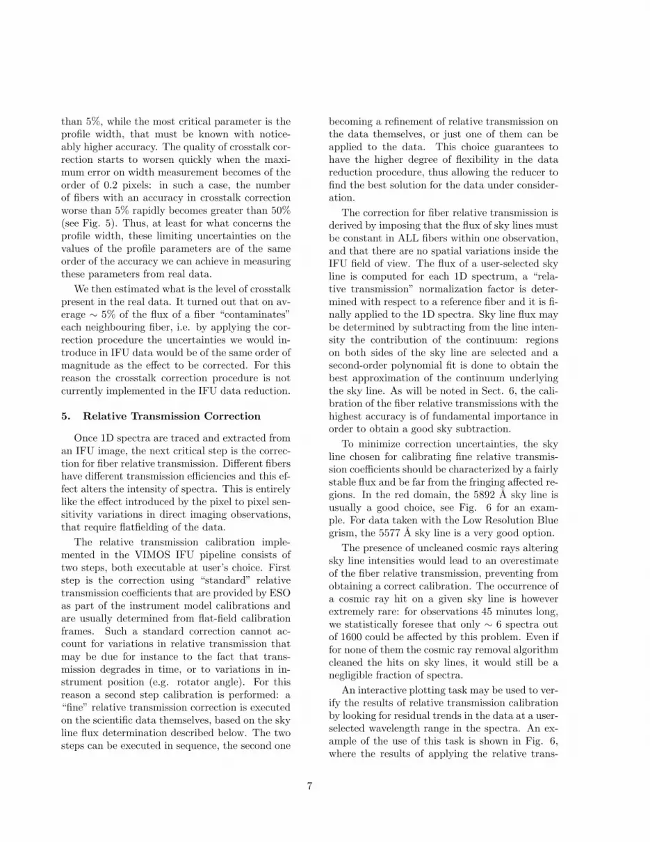
Given the adopted method for sky subtraction,an overall good relative transmission calibration isessential to get a correct intensity distribution andthus a proper selection of pure sky spectra. Onthe other hand, due to the median combination,if just some spectrum has not been perfectly cor-rected for fiber relative transmission, it will not af-fect the sky subtraction step. This sky subtractionprocedure guarantees good results, with the meanlevel over the continuum well centered around 0 inspectra where no object signal is present, and anrms of the order of a few percent. An example ofsky subtracted spectra can be seen in Fig. 8.

7. Flux calibration

The last step of data reduction on single obser-vations is flux calibration, done in a standard wayby multiplying 1D spectra by the sensitivity func-tion derived from standard star observations. Allthe spectra containing flux from the standard starare summed together, and the instrument sensi-tivity function computed by comparison with thereal standard star spectrum from the literature.

On the basis of a few objects with known mag-nitudes that have been observed with the VIMOSIFU, we have estimated that the overall absoluteflux accuracy that can be reached with a goodquality spectro-photometric calibration is of theorder of 15%, given the unavoidable sources of un-certainty, such as cross talk contribution (of theorder of 5%), relative transmission correction (be-tween 5% and 10%) and sky subtraction (few per-cents).

8. Final steps: jitter sequences data re-

duction

The final result of the single frame reductionprocedure is a FITS image, containing intermedi-ate products of the reduction (e.g. spectra notcorrected for fiber transmission, or not sky sub-tracted) under the form of image extensions, plus

some tables used and/or created during the exe-cution of the different tasks.

In many cases, observations had been carriedout using a jittering technique (the telescope isslightly offsetted from one exposure to the next).In these cases, the spectra from the single expo-sures must be stacked together according to theiroffsets, and in this process also correction for fring-ing can be applied.

8.1. Correcting for fringing

Due to the characteristics of the VIMOS CCDs,when observing in the red wavelength domain, onehas to deal with the fringing phenomenon, whoseeffects show up at wavelengths larger than ∼ 8200A in VIMOS spectra.

The decision to carry out the fringing correc-tion at the stacking of the single exposures stageis dictated by the consideration that during a typi-cal jitter sequence (a few hours exposure time) thefringing pattern remains relatively constant. Onthe contrary, the overall background intensity andthe relative strength of the individual sky emis-sion lines can vary significantly over the same timescales. Likewise, the physical location of the spec-tra on the CCD changes because of flexures (seeSect. 4.1 for an evaluation of flexures-induced im-age motions). Our approach has been to correctfirst for the most rapidly changing effects (firstspectra location, secondly sky background) andonly in the end to try to correct for fringing, whichis then computed and applied on 1D extractedspectra that have already been corrected for cos-mic ray hits, for relative fiber transmission, etc.

The fringing correction can only be applied onjittered observations and is performed separatelyfor the sets of images coming from different quad-rants.

First, all the spectra obtained in the jitter se-quence for a given fiber are combined without tak-ing into account telescope offsets: any object sig-nal is thus averaged out in the combination andwhat remains is a good representation of the fring-ing pattern, which is then subtracted from eachsingle spectrum.

The quality of fringing correction is very good:Fig. 9 shows the result of the reduction of a se-quence of 9 jittered exposures on the ChandraDeep Field South. Observations have been done

9

using the Low Resolution Red grism (wavelengthrange 5500−9500 A, dispersion 7.14 A/pixel), withsingle frame exposure times of 26 minutes. In Fig.9, top, the exposures have been combined withoutapplying any correction for fringing, while the bot-tom frame shows the result after having correctedfor fringing as explained above. It can be seen thatfringing correction is efficient in removing almostcompletely the residuals in the λ > 8200 A regionof the spectra.

8.2. Stacking jittered sequences of expo-

sures

Stacking is done using all the available imagesfrom all the VIMOS quadrants at a time. In fact,due to the contiguous field of view of the VIMOSIFU and given how fibers are rearranged on thefour VIMOS quadrants, an object spectrum can“move” from one quadrant to the other going fromone jittered exposure to the next.

Image stacking makes use of datacubes, i.e.3D images where the (x,y) axes sample the spa-tial coordinates and the z axis samples the wave-length. One datacube is created starting from thefour images of each IFU exposure. Jitter offsetsare computed by using the header information ontelescope pointing coordinates or by means of auser-given offset list, and are used to build a final3D image starting from single datacubes. Varia-tions of the relative transmission from quadrantto quadrant, and inside the same quadrant fromone exposure to the next one in the sequence, aretaken into account by properly rescaling image in-tensities.

The output of the reduction procedure is aFITS image containing all the stacked 1D spectrain the final datacube: each spectrum is writtenin a row of the output image (see Fig. 9), and acorrespondence table between the position of thespectrum in the final 3D cube appended to it.

Finally, a 2D reconstructed image can be builtfor scientific analysis. In Fig. 10 we show an exam-ple of 2D reconstructed image from VIMOS IFUobservations of the candidate cluster MRC1022-299 associated with a high redshift radiogalaxy(McCarthy et al. 1996; Chapman et al. 2000).A sequence of 5 jittered exposures of 26 minuteseach taken with the Low Resolution Red grism hasbeen combined and integrated over the wavelength

range 5800−8000 A (left) and over a narrow band100 A wide centered at 7100 A (right), where anemission line identified with OII is observed in theradiogalaxy spectrum. The radiogalaxy, invisiblein the broad-band image, shows up at the center ofthe field in the narrow-band image. From the OIIline we got a redshift of 0.9085 for the radiogalaxy,consistent with the value quoted by McCarthy etal. (1996).

2D reconstructed images can be built from anykind of 1D extracted spectra, e.g. transmissioncorrected or sky subtracted ones, by using the sky-to-CCD fiber correspondence given in the stan-dard IFU table or, in the case of a jitter sequencereduction, in the associated correspondence table.These images are particularly useful when deal-ing with crowded fields data, when the automaticsky subtraction recipe cannot guarantee good re-sults. In such cases the reduction to 1D spectracan be done without sky subtraction. A prelimi-nary 2D image can be reconstructed and used tointeractively identify fibers/spectra in object-freeregions, to be later combined to obtain an accurateestimate of the sky background signal.

9. Summary

The VIMOS Integral Field Spectrograph has re-quired a new approach to process the large amountof data produced by 6400 micro-lenses and fibers.

The instrumental IFU setup and the packingof spectra on the 4 VIMOS detectors has moti-vated the development of dedicated recipes, withthe possibility to carefully check the quality of re-sults by means of interactive tasks.

With the large amount of spectra acquired bythe VIMOS IFU, it has been mandatory to imple-ment the IFU data processing in a pipeline schemeas much automated as possible. The VIMOS IFUdata processing is implemented under the VIPGIenvironment (Scodeggio et al. 2005) and is avail-able to the scientific community to process VIMOSIFU data since November 2003.

We have estimated that the overall abso-lute flux accuracy that can be reached with ourpipeline is of the order of 15%, the main sourcesof uncertainty being the cross talk contribution(significant, of the order of 5%), the relative trans-mission correction (between 5% and 10%) and skysubtraction (few percents).

10

This research has been developed within theframework of the VVDS consortium.This work has been partially supported by theCNRS-INSU and its Programme National deCosmologie (France), and by Italian Ministry(MIUR) grants COFIN2000 (MM02037133) andCOFIN2003 (num.2003020150).This work has been partly supported by theEuro3D Research Training Network.The VLT-VIMOS observations have been carriedout on guaranteed time (GTO) allocated by theEuropean Southern Observatory (ESO) to theVIRMOS consortium, under a contractual agree-ment between the Centre National de la RechercheScientifique of France, heading a consortium ofFrench and Italian institutes, and ESO, to design,manufacture and test the VIMOS instrument.

REFERENCES

Allington-Smith, J. & Content, R. 1998, PASP,110, 1216

Allington-Smith, J. et al. 2002, Experimental As-tronomy, 13, 1

Bacon, R. et al. 1995, A&AS, 113, 347

Bacon, R. et al. 2001, MNRAS, 326, 23

Bonneville, C. et al. 2003, Proc. SPIE, 4841, 1771

Chapman, S. C., McCarthy, P. J., Persson, S. E.2000, AJ, 120, 1612

Content, R. M. et al. 2000, Proc.SPIE, 4013, 851

Emsellem, E. et al. 2004, MNRAS, 352, 721

Horne, K. 1986, PASP, 98, 609

Le Fevre, O. et al. 2002, The Messenger, 109, 21

McCarthy, P. J., Kapahi, V. K., van Breugel, W.Persson, S. E., Athreya, R., Subrahmanya, C.R. 1996, ApJS, 107, 19

Prieto, E., Le Fevre, O., Saisse, M., Voet, C., Bon-neville, C., 2000, Proc, SPIE, 4008, 510

Scodeggio, M. et al. 2005, PASP, submitted

Walsh, J. R. & Roth, M. M. 2002, The Messenger,109, 54

This 2-column preprint was prepared with the AAS LATEXmacros v5.2.

11

Table 1: Characteristics of the VIMOS Integral Field Unit.

Spectral resolution Field of View Spatial resolution Spatial elements Spectral elements(arcsec/fiber) (pixel)

Low (R ∼ 200) 54′′ × 54′′ 0.67 6400 60027′′ × 27′′ 0.33

High (R ∼ 2500) 27′′ × 27′′ 0.67 1600 409613′′ × 13′′ 0.33

12

2021 40

416061 80

1

1 2 53 4

1 2 53 4

1 2 53 4

1 2 53 4

1 80

A

B

C

D

Mask 3(a)

Quadrant 4 (to Mask 4)

Quadrant 1 (to Mask 1)

(c)

(b)

Quadrant 2 (to Mask 2)

Quadrant 3 (to Mask 3)

A

DB

2

1

3

4

5

1

3

2

4

5

C

5

4

3

2

1

5

4

3

2

1

D

C

B

A

Fig. 1.— Geometrical layout of the VIMOS Integral Field Unit. (a) The 80×80 microlenses array that formthe IFU head. Each quadrant is associated with a 1600 fibers bundle which conveys the collected light intoone of the four VIMOS channels. For clarity, only details for quadrants 1 and 3 are shown. Sub-bundlesgroup fibers associated with contiguous microlenses on each quadrant (the regions marked A, B, C, and D)and feed the four pseudo-slits on the special IFU masks put in the VIMOS focal plane. A fiber sub-bundleis in turn divided into 5 modules of 80 fibers each. The fibers in each module are aligned onto the pseudo-slits according to a complex pattern, as can be seen in (b). Panel (c) illustrates how the fiber modules areorganized over the pseudo-slits in the case of the IFU Mask no. 3.

13

sky lines

module

module

A

B

C

D

λ

Fig. 2.— Left: example of an IFU exposure, only one of four quadrants is shown, the four pseudo-slitswith 400 spectra each are visible. Each spectrum spans 5 pixels in the spatial direction. One fiber modulebelonging to pseudo-slit A is indicated in the left panel; a zoom on the 80 spectra coming from this moduleis shown in the right panel.

14

ScienceFrames

LampFrame

Instrument Model

InstrumentResponseDetermination

Instrument Calibrations

Observations

LocationSpectra

WavelengthCalibration

Spectra 1D Extraction

Spectra 2D Extraction

3D Data Cube

2D Image

Sequence Combination

Fringing Correction

Relative Transmission Calibration Sky Subtraction

Flux Calibration

Cosmic Ray Cleaning

Fig. 3.— Block diagram showing the various stepsof the reduction of VIMOS IFU data. Optionalsteps are marked in grey.

Fig. 4.— Sky line profile along the dispersion di-rection (continuum line), superimposed to the pro-file of a cosmic ray (dot-dashed line).

Fig. 5.— Performance of the crosstalk correctionas a function of the accuracy in the measure of thefiber profile width. Solid line: number of fiberswith error on the recovered flux less than 5%.Dashed line: error between 5% and 10%. Dottedline: error between 10% and 20%. Dot-dashed:error greater than 20%.

15

Fig. 6.— Graphical task for the analysis of the performance of relative transmission calibration for IFU data.The top panel shows the intensity of the 1600 spectra at the wavelength of the skyline that has been usedfor the calibration (in this example the 5892 A line, spectra taken with Low Resolution Red grism). Thebottom panel shows again the spectral intensity, this time computed in a user–selected continuum region at∼ 6000 A. The rms of the intensities is also shown for each panel.

16

Fig. 7.— Distribution of the 5892 A sky lineskewness as a function of sky line width, measuredfor ∼ 1600 1D spectra.

17

N. o

f sp

ectr

a

Wavelength (A)5500 6000 7000 8000 9000

N. o

f sp

ectr

a

Fig. 8.— Example of the results obtained by the sky subtraction procedure. Top: 1D relative transmissioncorrected spectra in an exposure taken with the Low Resolution Red grism. Bottom: same spectra after skysubtraction. The 5892 A sky line has been used to group spectra before “average” sky spectrum computation.In the ∼ 8500 A region the zero order due to a nearby pseudo-slit has been clipped, originating a “flat”intensity distribution.

18

5500 6000 7000 8000 9000

N. o

f sp

ectr

aN

. of

spec

tra

Wavelength (A)

Fig. 9.— Efficiency of fringing correction: example of jitter–combined fully reduced sequence of 9 exposures,26 minutes each, taken with the Low Resolution Red grism (wavelength range 5500−9500 A) on the ChandraDeep Field South. Each row is a different spectrum. Upper and lower panels are respectively without andwith fringing correction applied to the data. As it can be seen in the lower panel, at wavelengths larger than∼ 8200 A very low fringing residuals are left after correction.

19

Fig. 10.— 2D reconstructed image of the cluster MRC1022-299 obtained by integrating over the 5800÷8000A wavelength range (left) and over 100 A centered on the radiogalaxy [OII]3727 emission line (right) red-shifted at ≃ 7100 A (redshift z=0.9085). The radiogalaxy OII emission is clearly extended and asymmetric,and a velocity field can be retrieved from the 3D cube. On these images East is up and North is right. About3% of the pixels correspond to black/dead fiber spectra and have been cleaned with the IRAF task fixpix.

20