Seediscussions,stats,andauthorprofilesforthispublicationat:https://www.researchgate.net/publication/41712188

VLT-UVESanalysisof5giantsin47Tucanae

ARTICLEinASTRONOMYANDASTROPHYSICS·MAY2005

ImpactFactor:4.38·DOI:10.1051/0004-6361:20041634

CITATIONS

40

READS

32

11AUTHORS,INCLUDING:

S.Ortolani

UniversityofPadova

246PUBLICATIONS2,608CITATIONS

SEEPROFILE

YazanMomany

EuropeanSouthernObservatory

170PUBLICATIONS3,418CITATIONS

SEEPROFILE

ManuelaZoccali

PontificalCatholicUniversityofChile

237PUBLICATIONS4,244CITATIONS

SEEPROFILE

DanteMinniti

PontificalCatholicUniversityofChile

659PUBLICATIONS9,580CITATIONS

SEEPROFILE

Availablefrom:ManuelaZoccali

Retrievedon:03February2016

A&A 435, 657–667 (2005)DOI: 10.1051/0004-6361:20041634c© ESO 2005

Astronomy&

Astrophysics

VLT-UVES analysis of 5 giants in 47 Tucanae�,��

A. Alves-Brito1, B. Barbuy1, S. Ortolani2, Y. Momany2, V. Hill3, M. Zoccali4,5, A. Renzini6,D. Minniti4, L. Pasquini6, E. Bica7, and R. M. Rich8

1 Universidade de São Paulo, IAG, Rua do Matão 1226, Cidade Universitária, São Paulo 05508-900, Brazile-mail: [abrito;barbuy]@astro.iag.usp.br

2 Università di Padova, Dipartimento di Astronomia, Vicolo dell’Osservatorio 2, 35122 Padova, Italye-mail: ortolani@pd.astro.it

3 Observatoire de Paris-Meudon, 92195 Meudon Cedex, Francee-mail: Vanessa.Hill@obspm.fr

4 Universidad Catolica de Chile, Department of Astronomy & Astrophysics, Casilla 306, Santiago 22, Chilee-mail: [dante;mzoccali]@astro.puc.cl

5 Princeton University Observatory, Peyton Hall, Princeton, NJ 08544, USA6 European Southern Observatory, Karl Schwarzschild Strasse 2, 85748 Garching bei München, Germany

e-mail: [arenzini;lpasquin]@eso.org7 Universidade Federal do Rio Grande do Sul, Departamento de Astronomia, CP 15051, Porto Alegre 91501-970, Brazil

e-mail: bica@if.ufrgs.br8 UCLA, Department of Physics & Astronomy, 8979 Math-Sciences Building, Los Angeles, CA 90095-1562, USA

e-mail: rmr@astro.ucla.edu

Received 10 July 2004 / Accepted 10 January 2005

Abstract. High resolution spectra of 5 giants, including a horizontal branch star, of the metal-rich globular cluster 47 Tucanaewere obtained with the UVES spectrograph at the 8 m VLT UT2-Kueyen telescope. The atmospheric parameters (Teff , log g,[Fe/H], vt) were derived from VIJK photometry and spectroscopic data based on Fe I and Fe II lines. Fe I and Fe II iron abun-dances and respective total errors [Fe I/H]= –0.66 ± 0.12 and [Fe II/H]= –0.69 ± 0.24 are found. Abundances of α (O, Mg, Ca,Si, Ti), odd-Z (Na, Al), s- (Ba, La, Zr), and r-process (Eu) elements were determined by means of spectrum synthesis. The mainresults are [O/Fe] = +0.35 ± 0.11, [Mg/Fe]≈ [Si/Fe]≈ [Ti/Fe]=+0.23 ± 0.17, [Ca/Fe] = 0.0 ± 0.15, [Ba/Fe] = +0.31 ± 0.22and [Eu/Fe] = +0.33 ± 0.10. Overabundances of the α-elements O, Mg, Si and Ti, and of Eu are similar to those seen in halometal-poor stars, whereas a solar Ca-to-Fe ratio resembles the values found in bulge stars. An overall metallicity Z = 0.006 or[M/H]= –0.45 is thus obtained, as is a mean heliocentric radial velocity vhel

r = −22.43 ± 1.99 km s−1.

Key words. globular clusters: individual: 47 Tucanae – globular clusters: general – stars: abundances

1. Introduction

47 Tucanae is the second brightest globular cluster of ourGalaxy. Its distance is 4.5 kpc (Harris 1996, as updated athttp://physun.physics.mcmaster.ca/Globular.html).It is located at a high Galactic latitude J2000α = 00h24m05.19s, δ = −72o04′49.9′′ (l = 305.90◦,b = −44.89◦), and has a low reddening of E(B − V) = 0.04(Harris 1996). As a template metal-rich halo cluster, it is oftenconsidered as the prototype of a metal-rich globular cluster.Its metallicity of [Fe/H] = −0.7 (Harris 1996) is lower than

� Observations collected both at the European SouthernObservatory, Paranal and La Silla, Chile (ESO programmes65.L-0340, 65.L-0371, 67.D-0489 and 69.D-0582).�� Table A.1 is only available in electronic form at the CDS viaanonymous ftp to cdsarc.u-strasbg.fr (130.79.128.5) or viahttp://cdsweb.u-strasbg.fr/cgi-bin/qcat?J/A+A/435/657

more metal-rich bulge clusters such as NGC 6528, NGC 6553,NGC 6440, Terzan 5 and Liller 1, which show metallicitiesclose to the solar value (e.g. Barbuy et al. 1998, 1999a; Cohenet al. 1999; Carretta et al. 2001; Origlia et al. 2002; Meléndezet al. 2003; Zoccali et al. 2004). These more metal-rich clustersare templates for studies of elliptical galaxies (Bica 1988),whereas 47 Tuc is representative of the metal-rich componentof the bimodal metallicity distribution of globular clusters inexternal galaxies (see Geisler et al. 2002). Despite these inter-esting characteristics, there are not enough detailed analysesbased on high resolution and high S/N CCD spectroscopy ofindividual member stars available in the literature. The mainaim of this work is to derive precise abundances for giants of47 Tuc, as a reference for other work on metal-rich clusters. Tothis end, a detailed abundance analysis of five stars in 47 Tucusing high resolution échelle spectra obtained with UVES atthe ESO VLT-UT2 Kueyen telescope is presented.

Article published by EDP Sciences and available at http://www.edpsciences.org/aa or http://dx.doi.org/10.1051/0004-6361:20041634

658 A. Alves-Brito et al.: Analysis of 5 giants in 47 Tucanae

Brown & Wallerstein (1990, 1992) have used CCD highresolution échelle spectra to analyse 4 stars, two of them lo-cated on the Red Giant Branch (RGB) and the other two onthe Asymptotic Giant Branch (AGB). After finding a spreadin abundances, these authors discuss the possibility of primor-dial abundance variations. Norris & Da Costa (1995, hereafterNC95) analysed one cool giant based on high resolution spectra(R ∼ 38 000), as a comparison object in a study of ω Centaurigiants. Carretta et al. (2004, hereafter C04) used UVES@VLTto derive abundances of turn-off stars, with 3 dwarfs and 9 sub-giants; a metallicity [Fe/H] = −0.67, together with an over-abundance of α-elements of +0.3 dex were obtained, and nosignificant differences were found between the pattern shownby giants and their less evolved stars. James et al. (2004, here-after J04) derived the heavy element abundances using thesame spectra studied by C04.

The observations are described in Sect. 2, while the stellarparameters and abundances are derived in Sect. 3. Abundanceratios are discussed in Sect. 4, and conclusions drawn in Sect. 5.

2. The data

2.1. Imaging

B, V and I images of 47 Tuc were obtained in June 2002 withthe Wide-Field Imager (WFI) at the 2.2 m ESO-MPI telescope(La Silla, Chile). The data were obtained using our programdedicated to surveying the Galactic globular clusters with theWFI. The WFI camera consists of eight 2048 × 4096 EEV-CCDs with a total field of view of 34 × 33 arcmin2. The ex-posure times were divided into deep and shallow in order tosample both bright red giants and the faint main sequence. Allscientific images were dithered in such a way as to cover thegaps separating the eight 2048 × 4096 CCDs. The seeing con-ditions were generally good throughout the run. Basic reduc-tions of the CCD mosaic (de-biassing and flat-fielding) wereperformed using the IRAF package MSCRED (Valdes 1998).

Stellar photometry was performed using the DAOPHOTand ALLFRAME programs (Stetson 1994). Further details aregiven in Momany et al. (2002). The instrumental PSF magni-tudes were normalized to 1 s. exposure and zero airmass. Thesewere then converted into aperture magnitudes assuming thatmap = mPSF − const., where the constant is the aperture correc-tion.

The photometric calibrations were defined using standardUBVI stars from Landolt (1992). Secondary standard starsfrom Stetson (http://cadcwww.hia.nrc.ca/standards/)provided a larger number of standards. In a few cases thesebelonged to the same globular clusters that were to becalibrated. Calibration uncertainties in the BVI filters areestimated as 0.03, 0.03 and 0.04, respectively. In deriving thecalibration equations we assumed the following extinctioncoefficients for La Silla: KB = 0.23, KV = 0.16 and KI = 0.07(http://www.ls.eso.org/lasilla/atm_ext/). J, H andKS colours are from the 2MASS Atlas (Skrutskie et al. 1997),http://ipac.caltech.edu/2mass/releases/allsky/.Five individual stars were selected from our sample forspectroscopic observations. The location of target stars on the

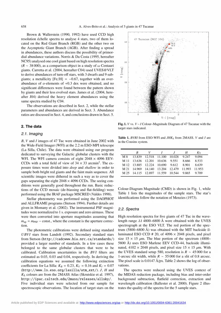
Fig. 1. V vs. V − I Colour–Magnitude Diagram of 47 Tucanae with thetarget stars indicated.

Table 1. BVRI from ESO-WFI and JHKS from 2MASS. V and I arein the Cousins system.

B V I J H KsM 8 13.839 12.518 11.100 10.028 9.247 9.094M 11 13.636 12.201 10.636 9.551 8.666 8.533M 12 13.885 12.224 10.690 9.612 8.901 8.639M 21 14.969 14.140 13.204 12.479 11.993 11.953M 25 14.115 12.897 11.559 10.544 9.865 9.709

Colour-Diagram Magnitude (CMD) is shown in Fig. 1, whileTable 1 lists the magnitudes of the sample stars. The star’sidentifications follow the notation of Menzies (1973).

2.2. Spectra

High resolution spectra for five giants of 47 Tuc in the wave-length range λλ 4800–6800 Å were obtained with the UVESspectrograph at the ESO VLT. The red portion of the spec-trum (5800–6800 Å) was obtained with the MIT backside il-luminated ESO CCD # 20, of 4096 × 2048 pixels, and pixelsize 15 × 15 µm. The blue portion of the spectrum (4800–5800 Å) uses ESO Marlene EEV CCD-44, backside illumi-nated, 4102 × 2048 pixels, and pixel size 15 × 15 µm. Withthe UVES standard setup 580, resolution is R ∼ 45 000 for a1-arcsec slit width, while R ∼ 55 000 for a slit of 0.8 arcsec.The pixel scale is 0.0147 Å/px. Table 2 shows the log of obser-vations.

The spectra were reduced using the UVES context ofthe MIDAS reduction package, including bias and inter-orderbackground subtraction, flatfield correction, extraction andwavelength calibration (Ballester et al. 2000). Figure 2 illus-trates the quality of the spectra for the 5 sample stars.

Article published by EDP Sciences and available at http://www.edpsciences.org/aa or http://dx.doi.org/10.1051/0004-6361:20041634

A. Alves-Brito et al.: Analysis of 5 giants in 47 Tucanae 659

Table 2. Log of the spectroscopic observations carried out in 24–26 June 2000 and 6 July 2001. The quoted seeing are mean values along theexposures. For star M21 the S/N was obtained based on a spectrum smoothed with a gaussian of σ = 3 pixels.

star α2000 δ2000 date/ UT exp Seeing Airmass (S/N)/px Slit vobsr vhel.

r

Julian Day (min) (′′) width km s−1 km s−1

M 8 00:26:28.8 –71:50:12 24.06.00 09:31 45 1.2 1.5 280@6218Å 0.8 –34.67 –28.16245171904.07.01 09:24 30 0.8 “ 245@6461Å 0.8 –34.67 –28.162452094

M 11 00:26:57.7 –71:49:10 04.07.01 09:43 25 0.8 “ 241@6329Å 0.8 –25.89 –19.292452094

M 12 00:26:27.1 –71:47:40 04.07.01 09:04 15 0.8 “ 247@6329Å 0.8 –29.34 –22.802452094

M 21 00:25:57.2 –71:49:28 05.07.01 09:22 35 1.5 “ 213@6460Å 0.8 –23.28 –16.972452095

M 25 00:24:47.2 –71:47:44 25.06.00 09:46 30 1.5 “ 258@6401Å 1.0 –33.19 –24.962451720

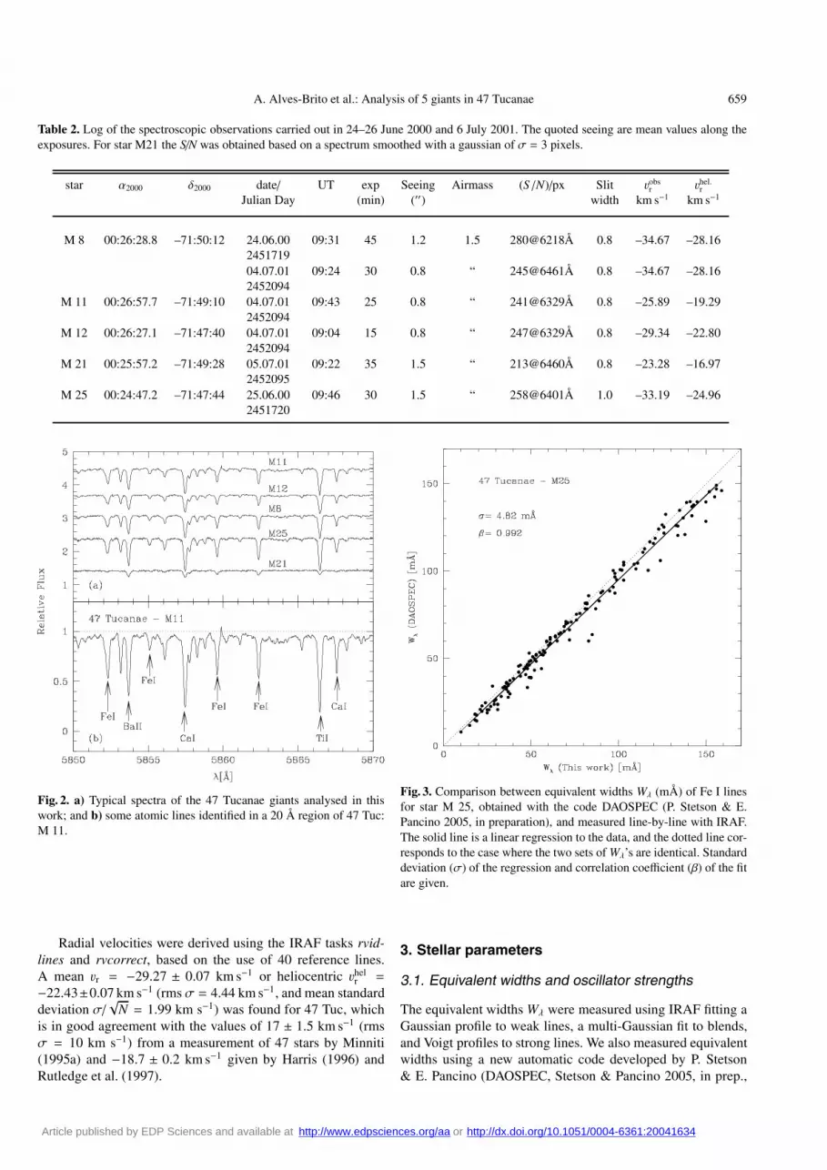
Fig. 2. a) Typical spectra of the 47 Tucanae giants analysed in thiswork; and b) some atomic lines identified in a 20 Å region of 47 Tuc:M 11.

Radial velocities were derived using the IRAF tasks rvid-lines and rvcorrect, based on the use of 40 reference lines.A mean vr = −29.27 ± 0.07 km s−1 or heliocentric vhel

r =

−22.43±0.07 km s−1 (rms σ = 4.44 km s−1, and mean standarddeviation σ/

√N = 1.99 km s−1) was found for 47 Tuc, which

is in good agreement with the values of 17 ± 1.5 km s−1 (rmsσ = 10 km s−1) from a measurement of 47 stars by Minniti(1995a) and −18.7 ± 0.2 km s−1 given by Harris (1996) andRutledge et al. (1997).

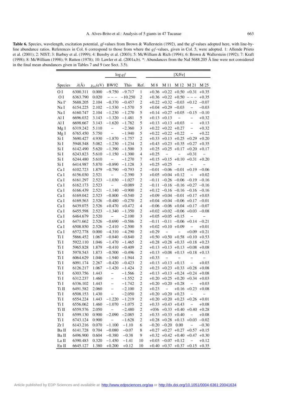
Fig. 3. Comparison between equivalent widths Wλ (mÅ) of Fe I linesfor star M 25, obtained with the code DAOSPEC (P. Stetson & E.Pancino 2005, in preparation), and measured line-by-line with IRAF.The solid line is a linear regression to the data, and the dotted line cor-responds to the case where the two sets of Wλ’s are identical. Standarddeviation (σ) of the regression and correlation coefficient (β) of the fitare given.

3. Stellar parameters

3.1. Equivalent widths and oscillator strengths

The equivalent widths Wλ were measured using IRAF fitting aGaussian profile to weak lines, a multi-Gaussian fit to blends,and Voigt profiles to strong lines. We also measured equivalentwidths using a new automatic code developed by P. Stetson& E. Pancino (DAOSPEC, Stetson & Pancino 2005, in prep.,

Article published by EDP Sciences and available at http://www.edpsciences.org/aa or http://dx.doi.org/10.1051/0004-6361:20041634

660 A. Alves-Brito et al.: Analysis of 5 giants in 47 Tucanae

Table 3. Dereddened colours. J: Johnson, TCS: Telescope CarlosSanches, C: Cousins, CIT: California Institute Technology.

Star (V − I)0 (V − K)0 (J − K)0 (V − I)0 (V − K)0 (J − K)0

(J) (TCS) (TCS) (C) (CIT) (CIT)

M 8 1.754 3.306 0.873 1.365 3.290 0.875M 11 1.943 3.550 0.954 1.512 3.534 0.955M 12 1.903 3.467 0.911 1.481 3.451 0.912M 21 1.134 2.072 0.481 0.883 2.053 0.489M 25 1.654 3.071 0.778 1.284 3.054 0.782

http://cadcwww.hia.nrc.ca/stetson/daospec/), asshown in Fig. 3 for 10 < Wλ < 160 mÅ.

The Fe line list and respective oscillator strengths from theNational Institute of Standards & Technology (NIST) library(Martin et al. 2002) were adopted, along with Fe II oscillatorstrengths renormalized by Meléndez & Barbuy (2005). The listof Fe I and Fe II lines is given in Table A.1.

Damping constants for neutral lines were computed usingthe collisional broadening theory of Barklem et al. (1998,2000, and references therein), as described in Zoccali et al.(2004) and Coelho et al. (2005). The oscillator strengths forelements other than Fe were obtained by fitting the solarspectrum observed with the same VLT-UVES instrumentation(www.eso.org/observing/dfo/quality/UVES/pipeline/solar_spectrum.html) and the Arcturus spectrum (Hinkleet al. 2000) for different literature gf-values, as described inZoccali et al. (2004). The adopted gf-values were selected bychoosing the best fit to the solar and Arcturus spectra and areindicated in Table 6. In order to illustrate the reliability of theatomic constants, in Fig. 7 we show the CaI 6455.5 Å linefor the solar, Arcturus, and 47 Tuc: M 12 spectra. Table 6also reports gf-values used by Brown & Wallerstein (1992),in order to assess possible abundance discrepancies resultingfrom differences in gf-values. For the oxygen forbidden line[OI] 6300.311 Å we adopt the oscillator strength derived byAllende Prieto et al. (2001) of log g f = −9.716. The NiI linethat blends the [OI] line is included in the line list, but its effectis negligible in K giants.

For lines of the heavy elements BaII, LaII, and EuII, a hy-perfine structure was taken into account, based on the hyper-fine constants by Lawler et al. (2001a) for EuII, Lawler et al.(2001b) for LaII, and Biehl (1976) for BaII, where a solar iso-topic mix is adopted, and a code described and made availableby McWilliam (1998) is employed.

Solar abundances were adopted from Grevesse & Sauval(1998), except that of oxygen, where the value ε(O) = 8.77of Allende Prieto et al. (2001), suitable for the use of 1-Dmodel atmospheres was used. For europium, the updated valueis ε(Eu)= 0.54.

3.2. Temperatures

A reddening E(B − V) = 0.04 for 47 Tuc (Harris 1996) andreddening laws E(V − I)/E(B − V)= 1.33 (Dean et al. 1978),E(V − K)/E(B − V)= 2.744, and E(J − K)/E(B − V)= 0.52

(Rieke & Lebofsky 1985) were all adopted, and the dereddenedcolours are given in Table 3.

Photometric temperatures were derived from V, I, J,K mag-nitudes, adopting the colour-temperature calibrations of Alonsoet al. (1999, 2001 hereafter AAM99) and Houdashelt et al.(2000, hereafter HBS00). Table 4 gives the effective temper-atures derived from V − I, V − K, and J − K colours usingthe two calibrations. The photometric Teff values given by theV − K colour using the AAM99 calibration were adopted, asrepresentative of the photometric indicators. The effective tem-peratures were then checked by imposing excitation equilib-rium for Fe I and Fe II lines of different excitation potential, asillustrated in Fig. 4 and given in Table 5. Spectroscopic tem-peratures are about 50 K hotter than photometric ones. For thehotter Horizontal Branch (HB) star M 21, we were able to de-rive the temperature from the Hα profile T (Hα) (Fig. 5).

3.3. Gravities

The classical relation log g∗ = 4.44+4 log(T∗/T�)+0.4(Mbol−4.75) + log(M∗/M�) was used, adopting T� = 5780 K, M∗ =0.80 M� and Mbol� = 4.75 (Cram 1999). A distance modu-lus of (m − M)V = 13.27 (Zoccali et al. 2001), a reddening ofE(B − V) = 0.04 and AV = 0.124, together with bolometriccorrection BCV values from AAM99 were used to derive pho-tometric gravities, from the classical formula above, which aregiven in Tables 4 and 5. We also derived log g from 12.5 Gyrisochrones of Z = 0.0054, Y = 0.24, [Fe/H] = −0.76, and[α/Fe]=+0.3 by Kim et al. (2002). These gravity values, re-ported in Table 4, are higher than the photometric ones derivedby using the classical relation, by ∆ log g = 0.11. Finally, wederived log g from ionization equilibrium of Fe I and Fe II lines(Table 4). In the following, the spectroscopic effective temper-atures and gravities are assumed.

3.4. Iron abundance

The set of equivalent widths measured with IRAF were usedin the following, and Fe I and Fe II lines with 10 < Wλ <160 mÅ were selected. Photospheric 1D models for the samplegiants were extracted from the NMARCS grid (Plez et al. 1992)originally developed by Bell et al. (1976) and Gustafsson et al.(1975). The LTE abundance analysis and spectrum synthesiscalculations were performed with the codes by Spite (1967, andsubsequent improvements in the last thirty years), described inCayrel et al. (1991) and Barbuy et al. (2003).

Stellar parameters were derived by initially adopting thephotometric effective temperature and gravity, and then furtherconstraining both the temperature by imposing excitation equi-librium for Fe lines and the gravity by imposing ionizationequilibrium for Fe and Fe . Microturbulence velocity vt wasdetermined by canceling the trend of Fe I abundance vs. equiv-alent width. Figures 6a,b show the derived Fe abundances as afunction of reduced equivalent width for stars M 8 and M 11.

The final values used in the analysis are the spectroscopicparameters Teff, log g, vt, [Fe /H] and [Fe /H] values reportedin Table 5, with the exception of Teff = T (Hα) adopted for

Article published by EDP Sciences and available at http://www.edpsciences.org/aa or http://dx.doi.org/10.1051/0004-6361:20041634

A. Alves-Brito et al.: Analysis of 5 giants in 47 Tucanae 661

Table 4. Photometric effective temperatures Teff derived using V − I, V − K and J − K based on relations by AAM99 and HSB00, absolutemagnitudes MV , bolometric corrections BCV , bolometric magnitudes Mbol and gravity values derived.

AAM99 HBS00 AAM99

Star TV−I TV−K TJ−K 〈T 〉 TV−I TV−K TJ−K 〈T 〉 MV CB(V) Mbol log gphoto log gKim log gion

M 8 4106 4036 3970 4037 ± 39 4150 4082 3956 4063 ± 57 −0.700 −0.869 −1.569 1.19 1.29 1.48M11 3933 3920 3813 3888 ± 38 4003 3972 3767 3914 ± 74 −1.017 −1.025 −2.042 0.95 1.03 1.20M12 3966 3957 3895 3939 ± 22 4028 4006 3866 3966 ± 51 −0.994 −0.971 −1.965 1.00 1.02 1.45M21 5000 5017 5099 5038 ± 30 5080 5091 5163 5111 ± 26 +0.922 −0.263 +0.659 2.46 – 2.46M25 4217 4166 4181 4188 ± 15 4259 4216 4201 4225 ± 17 −0.321 −0.734 −1.055 1.45 1.57 1.65

Fig. 4. Excitation equilibrium temperature derived by imposing aconstant abundance of Fe I as a function of the excitation potentialχex(eV), for stars M 8 and M 11.

M21. The mean iron abundances derived are [Fe I/H]= –0.66and [Fe II/H]= –0.69, with the latter value adopted in the fol-lowing Sections.

3.5. Abundance ratios

Elemental abundances were obtained through line-by-linespectrum synthesis calculations for the line list given in Table 6.The calculations of synthetic spectra were carried out usingthe code described in Barbuy et al. (2003), where constantsfor atomic lines are outlined in Sect. 3.1 and molecular linesof CN A2Π–X2Σ, C2 Swan A3Π–X3Π, TiO A3Φ–X3∆ γ andB3Π–X3∆ γ’ systems are taken into account.

Table 7 gives the final mean results for each star andthe mean for the 5 stars, whereas Table 8 reports the er-rors (Sect. 3.6). The results given in Table 7 indicate thatthe α-elements Mg, Si, and Ti are enhanced by [Mg, Si,Ti/Fe]≈+0.25, whereas [O/Fe]=+0.35, and [Ca/Fe]≈ 0.0.Figure 8b illustrates the fit of synthetic spectra to the observedone, whereas Fig. 8a shows the location of telluric lines,

indicating that the [OI]6300 Å line is free of blending withthem. The r-process element Europium is overabundant, with[Eu/Fe]= 0.33, compatible with the high α-element enhance-ments.

The abundance of Na derived from the NaI 5688.205 Åline is not considered in the final mean abundance, given thatit is clearly subject to non-LTE effects (Gratton et al. 1999),whereas such effects are negligible on the NaI 6154/6161 dou-blet (Takeda et al. 2003). The Ba abundance for M21 was notconsidered in the final mean for the cluster of [Ba/Fe]= 0.31,since it appears anomalous. [La, Zr/Fe]≈ 0.0, as expected fors-elements in old populations.

Table 9 compares the present results and those of BW92,NC95, C04 and J04. There is good agreement with C04, as wellas with J04 for Ba and Eu, particularly Ba. Note that the resultsby J04 were reported separately for subgiants and turn-off stars,and we adopted a mean of their results. The differences seenwith BW92 appear to be due mostly to their lower iron abun-dance, but also to differences in adopted gf-values (see Table 6).NC95 indicated enhancements of α-elements, in rather goodagreement with the present results. However their Eu abun-dance clearly disagrees with BW92, J04, and our results. NC95also find very low [Eu/Fe] values for their ω Cen giants; there-fore, there is probably a mistaken oscillator strength used intheir calculations.

3.6. Errors

3.6.1. Equivalent widths

Figure 3 shows the dispersionσ = 4.82 mÅ between the sets ofequivalent widths measured with DAOSPEC and IRAF. Aftercomparing the set of equivalent widths for two sample starswith similar atmospheric parameters (Teff:log g:[Fe/H]), M 8(4086:1.48:–0.62) and M 12 (4047:1.45:-0.63), σ = 4.55 mÅis obtained. Supposing that the two sets of measurements aresusceptible to the same error sources, a typical uncertainty inthe equivalent widths of σ = 3.22 mÅ is deduced, which canbe taken as a realistic estimation of uncertainty for all stars inthe sample.

Using the Cayrel (1988) equation, σWλ =1.5S/N

√ωδx,

(where σWλ is the uncertainty for Wλ, S/N [pix−1] the signal-to-noise ratio, ω [Å] the FWHM, and δx the pixel size), fortypical values of this work, we estimate an uncertainty ofσWλ = 0.3 mÅ. This represents an uncertainty smaller than 3%

Article published by EDP Sciences and available at http://www.edpsciences.org/aa or http://dx.doi.org/10.1051/0004-6361:20041634

662 A. Alves-Brito et al.: Analysis of 5 giants in 47 Tucanae

Table 5. Final atmospheric parameters.

Photometric Spectroscopic

Star T log g [Fe/H] [Fe/H] vt Texc THα log g [Fe/H] [Fe/H]

(K) (cm s−2) (I) (II) (km s−1) (K) (K) (cm s−2) (I) (II)

M 8 4036 1.19 –0.67 –0.75 1.42 4086 – 1.48 –0.62 –0.65

M 11 3920 0.95 –0.67 –0.72 1.49 3945 – 1.20 –0.62 –0.62

M 12 3957 1.00 –0.71 –0.79 1.45 4047 – 1.45 –0.63 –0.68

M 21 5017 2.46 –0.79 –0.81 1.42 5032 5100 2.46 –0.77 –0.82

M 25 4166 1.45 –0.67 –0.73 1.37 4200 – 1.65 –0.64 –0.67

Fig. 5. Hα profile for the star M 21 showing the wings for Teff = 5000,5100 (best fit), and 5200 K.

for the weaker lines (Wλ = 10 mÅ) and smaller than 1% for thestronger lines (Wλ = 160 mÅ). Note, however, that the equa-tion above does not consider uncertainties regarding the preciselocation of continuum, such that the value of σWλ is underesti-mated.

3.6.2. Atmospheric parameters

(i) Teff : the differences in effective temperatures derived fromthe different indicators (Tables 4 and 5) show errors within±100 K. (ii) log g: the surface gravity log g(Teff, M∗, Mbol) isaffected by errors on Teff (σTeff = 100 K), M∗ (σM∗ = 0.1 M�),and Mbol (σMbol = 0.07 mag), giving ±0.10 dex. By consider-ing the mean differences between the photometric and spectro-scopic gravities (Table 4), the uncertainty on log g is ±0.2 dex.(iii) vt: the rms of the data points of excitation equilibrium(Fig. 6) shows an uncertainty of the order of 0.2 km s−1 on themicroturbulence velocity. (iv) [Fe/H]: Table 8 reports theuncertainties on the derivation of abundances, obtained by

Fig. 6. [Fe I/H] vs. reduced equivalent width for stars M 8 and M 11.The dotted line corresponds to mean abundance obtained.

computing the results for ∆Teff = 100 K, ∆ log g = 0.2 and∆vt = 0.2 km s−1. The total error is given in the last column.

4. Discussion

Zinn (1985) proposed subdividing the globular cluster systeminto two subsystems: (i) the halo clusters, more metal-poor than[Fe/H]< –0.8, with a spherical distribution and a small rota-tional velocity, and (ii) the disk clusters containing those of[Fe/H]> –0.8 with a highly flattened distribution. In his study,47 Tuc is classified as a disk cluster. Armandroff (1989) ar-gued that the metal-rich clusters are associated with the thickdisk. More recently, Minniti (1995b) and Côté (1999) arguedthat based on their dynamics the metal-rich clusters in the in-ner spheroid are associated with the galactic bulge rather thanwith the disk, as already proposed earlier by Frenk & White(1982). Barbuy et al. (1999b) discussed the properties of clus-ters within 4 kpc of the Galactic bulge. In the bulge and halosubdivision, 47 Tuc would rather belong to the halo system. Itis located far from the bulge at RGC = 7.4 kpc and is high in

Article published by EDP Sciences and available at http://www.edpsciences.org/aa or http://dx.doi.org/10.1051/0004-6361:20041634

A. Alves-Brito et al.: Analysis of 5 giants in 47 Tucanae 663

Table 6. Species, wavelength, excitation potential, gf-values from Brown & Wallerstein (1992), and the gf-values adopted here, with line-by-line abundance ratios. References in Col. 6 correspond to those from where the g f -values, given in Col. 5, were adopted. 1: Allende Prietoet al. (2001); 2: NIST; 3: Barbuy et al. (1999); 4: Bensby et al. (2003); 5: McWilliam & Rich (1994); 6: Brown & Wallerstein (1992); 7: Kraft(1998); 8: McWilliam (1998); 9: Rutten (1978); 10: Lawler et al. (2001a,b). *: Abundances from the NaI 5688.205 Å line were not consideredin the final mean abundances given in Tables 7 and 9 (see Sect. 3.5).

log g f [X/Fe]

Species λ(Å) χex(eV) BW92 This Ref. M 8 M 11 M 12 M 21 M 25

O I 6300.311 0.000 −9.750 −9.717 1 +0.36 +0.22 +0.50 +0.31 +0.35O I 6363.790 0.020 − − − −10.250 2 +0.36 +0.22 +0.50 − − − +0.35

Na I∗ 5688.205 2.104 −0.370 −0.457 2 +0.22 +0.32 −0.03 +0.12 −0.07Na I 6154.225 2.102 −1.530 −1.570 5 +0.04 +0.29 −0.03 − −0.03Na I 6160.747 2.104 −1.230 −1.270 5 +0.14 +0.27 +0.05 −0.15 −0.10Al I 6696.032 3.143 −1.320 −1.481 5 +0.13 +0.13 − − +0.32Al I 6698.667 3.143 −1.620 −1.782 5 +0.13 +0.13 +0.03 − +0.13Mg I 6319.242 5.110 − −2.360 3 +0.22 +0.22 +0.27 − +0.32Mg I 6765.450 5.750 − −1.940 5 +0.22 +0.22 +0.22 − +0.22Si I 5690.427 4.930 −1.870 −1.757 2 +0.33 +0.13 +0.25 +0.29 +0.20Si I 5948.548 5.082 −1.230 −1.234 2 +0.43 +0.23 +0.35 +0.27 +0.35Si I 6142.490 5.620 −1.390 −1.500 3 +0.25 +0.25 +0.17 +0.20 +0.17Si I 6243.823 5.610 −1.150 −1.300 4 +0.25 − − +0.31 −Si I 6244.480 5.610 − −1.270 7 +0.15 +0.15 +0.10 +0.31 +0.20Si I 6414.987 5.870 −0.890 −1.128 3 +0.25 +0.25 − − −Ca I 6102.723 1.879 −0.790 −0.793 2 −0.01 −0.06 −0.01 +0.19 −0.06Ca I 6156.030 2.521 − −2.390 3 +0.05 +0.04 +0.12 − +0.02Ca I 6161.297 2.523 −1.030 −1.027 2 −0.11 −0.26 −0.06 −0.19 −0.16Ca I 6162.173 2.523 − −0.089 2 −0.11 −0.16 −0.16 +0.27 −0.16Ca I 6166.439 2.521 −1.140 −0.900 2 +0.12 −0.16 −0.16 −0.16 −0.16Ca I 6169.042 2.523 −0.800 −0.540 2 +0.09 +0.04 −0.01 +0.17 +0.03Ca I 6169.563 2.526 −0.480 −0.270 2 +0.04 +0.04 −0.06 +0.17 −0.01Ca I 6439.075 2.526 +0.470 +0.472 4 −0.06 −0.06 +0.04 +0.17 −0.07Ca I 6455.598 2.523 −1.340 −1.350 2 +0.02 +0.02 −0.06 +0.03 −0.08Ca I 6464.679 2.520 − −2.100 3 +0.05 +0.05 +0.15 − −Ca I 6471.662 2.526 −0.690 −0.586 2 −0.11 −0.11 −0.06 +0.14 −0.21Ca I 6508.850 2.526 −2.410 −2.500 5 +0.02 +0.10 +0.09 − +0.01Ca I 6572.778 0.000 −4.310 −4.290 2 +0.29 − − +0.09 +0.21Ti I 5866.452 1.067 −0.840 −0.840 2 +0.50 +0.50 +0.58 +0.10 +0.53Ti I 5922.110 1.046 −1.470 −1.465 2 +0.28 +0.28 +0.33 +0.18 +0.23Ti I 5965.828 1.879 −0.410 −0.409 2 +0.13 +0.13 +0.13 +0.08 +0.08Ti I 5978.543 1.873 −0.500 −0.496 2 +0.13 +0.08 +0.13 +0.18 +0.13Ti I 6064.629 1.046 −1.940 −1.944 2 +0.33 − − − −Ti I 6091.174 2.267 −0.420 −0.423 2 +0.13 +0.13 +0.13 − +0.03Ti I 6126.217 1.067 −1.420 −1.424 2 +0.23 +0.23 +0.33 +0.28 +0.08Ti I 6303.756 1.443 − −1.566 2 +0.13 +0.13 +0.24 +0.24 +0.08Ti I 6312.237 1.460 − −1.552 2 +0.20 +0.25 +0.20 +0.34 +0.03Ti I 6336.102 1.443 − −1.742 2 +0.20 +0.20 +0.28 − +0.03Ti II 6491.582 2.060 − −2.100 2 +0.23 − +0.16 +0.23 +0.08Ti I 6508.153 1.430 − −2.050 2 +0.20 +0.20 +0.23 − −Ti I 6554.224 1.443 −1.220 −1.219 2 +0.20 +0.20 +0.23 +0.26 +0.01Ti I 6556.062 1.460 −1.070 −1.075 2 +0.33 +0.43 +0.43 − +0.08Ti II 6559.576 2.050 − −2.480 2 +036 +0.33 +0.40 +0.40 +0.28Ti I 6599.130 0.900 −2.090 −2.085 2 +0.33 +0.33 +0.40 − +0.08Ti I 6743.124 0.900 − −1.628 2 +0.28 +0.28 +0.13 +0.03 −0.02Zr I 6143.216 0.070 −1.100 −1.10 6 −0.20 −0.20 0.00 − −0.30Ba II 6141.728 0.704 −0.080 −0.07 8 +0.27 +0.27 +0.27 +0.57 +0.15Ba II 6496.900 0.604 −0.380 −0.38 9 +0.32 +0.42 +0.40 +0.47 +0.30La II 6390.483 0.320 −1.450 −1.41 10 +0.03 −0.07 +0.12 − +0.12Eu II 6645.127 1.380 +0.200 +0.12 10 +0.40 +0.37 +0.37 +0.15 +0.35

Article published by EDP Sciences and available at http://www.edpsciences.org/aa or http://dx.doi.org/10.1051/0004-6361:20041634

664 A. Alves-Brito et al.: Analysis of 5 giants in 47 Tucanae

Table 7. Mean abundance values and internal error σ for the 5 sample stars of 47 Tucanae.

M 8 M 11 M 12 M 21 M 25

Species log ε�(X) N [X/Fe] N [X/Fe] N [X/Fe] N [X/Fe] N [X/Fe]

O I 8.77 2 +0.36 2 +0.22 2 +0.50 1 +0.31 2 +0.35Na I 6.33 2 +0.09 ± 0.05 2 +0.28 ± 0.01 2 0.01 ± 0.04 1 –0.15 2 –0.07 ± 0.03Al I 6.47 2 +0.13 2 +0.13 1 +0.03 * – 2 +0.22 ± 0.04Mg I 7.58 2 +0.22 2 +0.22 2 +0.24 ± 0.02 * – 2 +0.27 ± 0.05Si I 7.55 6 +0.28 ± 0.10 5 +0.20 ± 0.04 5 +0.22 ± 0.11 5 +0.27 ± 0.04 4 +0.23 ± 0.08Ca I 6.36 13 +0.02 ± 0.11 12 –0.04 ± 0.10 12 –0.01 ± 0.10 10 +0.09 ± 0.16 12 –0.05 ± 0.10Ti I 5.02 15 +0.24 ± 0.12 14 +0.24 ± 0.11 14 +0.27 ± 0.11 9 +0.19 ± 0.09 13 +0.10 ± 0.14Ti II 5.02 2 +0.29 ± 0.08 1 +0.33 2 +0.28 ± 0.17 2 +0.31 ± 0.11 2 +0.18 ± 0.14Zr I 2.60 1 –0.20 1 –0.20 1 +0.00 – – 1 –0.30Ba II 2.13 2 + 0.30 ± 0.03 2 + 0.35 ± 0.10 2 + 0.34 ± 0.08 2 + 0.52 ± 0.07 2 + 0.23 ± 0.11La II 1.22 1 +0.03 1 -0.07 1 +0.12 – – 1 +0.12Eu II 0.54 1 +0.40 1 + 0.37 1 +0.37 1 +0.15 1 +0.35

[Fe/H]

Fe I 7.51 122 −0.62 ± 0.11 113 −0.62 ± 0.11 119 −0.63 ± 0.11 124 −0.77 ± 0.11 130 −0.64 ± 0.11Fe II 7.51 13 −0.65 ± 0.11 14 −0.62 ± 0.15 14 −0.68 ± 0.11 12 −0.82 ± 0.10 15 −0.67 ± 0.15

Fig. 7. Computed CaI 6455.5 Å line for the solar, Arcturus and 47 Tuc:M 12 spectra, illustrating the reliability of the atomic constants.

the plane at Z ∼ 3 kpc, it belongs to neither the disk nor thebulge; on the other hand, it has a low eccentricity orbit and ro-tates around the Galaxy at 161 km s−1 to 191 km s−1 (Dinescuet al. 1999; Dauphole et al. 1996).

In the following we try to use the abundance ratios de-rived in this work as indicators of stellar population sig-natures. A low [Ca/Fe]= 0.0 is compatible with the low[Ca/Fe]≈+0.14 found in bulge field stars by MR94 and with[Ca/Fe]≈ –0.4 in stars of the bulge cluster NGC 6528 (Zoccaliet al. 2004). A high [Ba/Fe]=+0.31 is compatible with highvalues of [Ba/Fe]=+0.34 and +0.60 found for M 71 by

Table 8. Abundance uncertainties for a∆Teff = 100 K,∆ log g = +0.2,∆vt = 0.2 km s−1 and corresponding total error.

Abundance ∆T ∆log g ∆vt (∑

x2)1/2

( 100 K) (+ 0.2 dex) (+ 0.2 km s−1)(1) (2) (3) (4) (5)

M11

[Fe/H](I) −0.02 +0.04 −0.09 0.10[Fe/H](II) −0.19 +0.13 −0.05 0.23[O/Fe] +0.01 +0.05 −0.01 0.05[Na/Fe] +0.06 +0.11 −0.07 0.14[Al/Fe] +0.07 0.00 −0.03 0.08[Mg/Fe] +0.10 +0.14 −0.03 0.17[Si/Fe] −0.09 +0.06 −0.01 0.11[Ca/Fe] +0.10 +0.01 −0.10 0.14[Ti/Fe] +0.13 +0.04 −0.08 0.16[Zr/Fe] +0.19 +0.05 −0.08 0.21[Ba/Fe] +0.01 +0.07 −0.20 0.21[La/Fe] +0.01 +0.06 −0.03 0.07[Eu/Fe] −0.01 +0.08 −0.01 0.08

M21

[Fe/H](I) +0.09 −0.01 −0.06 0.11[Fe/H](II) −0.13 +0.09 −0.06 0.17

Ramírez & Cohen (2002), and for M 4 by Ivans et al. (1999),clusters that have comparably high metallicities of [Fe/H]=−0.71 and –1.18, respectively. Figure 9 shows the abun-dance pattern of 47 Tuc compared to those of M 71 and M 4.Therefore, in terms of [Ba/Fe], 47 Tuc behaves like other

Article published by EDP Sciences and available at http://www.edpsciences.org/aa or http://dx.doi.org/10.1051/0004-6361:20041634

A. Alves-Brito et al.: Analysis of 5 giants in 47 Tucanae 665

Fig. 8. a) Spectra of the reference B star HR 7316 (solid line), wherethe telluric lines are identified (⊕), and 47 Tuc:M12 (dotted line) show-ing that the [OI] line is free of blends with telluric ones. b) Observedspectrum compared to synthetic spectrum: [O/Fe]= 0.4 (dashed line),0.5 (solid line) and 0.6 (dotted line).

Table 9. Mean abundances obtained compared with results by Brown& Wallerstein (1992), Norris & Da Costa (1995), Carretta et al. (2004)and James et al. (2004).

[X/Fe] This work BW92 NC95 C04/J04

[Fe/H](I) −0.66 ± 0.07 −0.80 −0.72 −0.67[Fe/H](II) −0.69 ± 0.07 − −0.51 −[O/Fe] +0.35 ± 0.10 +0.43 +0.17 +0.23[Na/Fe] +0.03 ± 0.11 +0.11 +0.21 +0.23[Al/Fe] +0.13 ± 0.08 +0.67 +0.38 +0.23[Mg/Fe] +0.24 ± 0.04 +0.49 +0.29 +0.40[Si/Fe] +0.24 ± 0.02 +0.39 +0.34 +0.30[Ca/Fe] 0.00 ± 0.04 +0.06 +0.16 +0.20[TiI/Fe] +0.21 ± 0.07 +0.16 +0.27 +0.26[TiII/Fe] +0.28 ± 0.04 +0.16 +0.56 +0.38[Zr/Fe] −0.17 ± 0.12 −0.22 − −[Ba/Fe] +0.31 ± 0.07 −0.22 −0.04 +0.29[La/Fe] +0.05 ± 0.10 +0.24 −0.38 −[Eu/Fe] +0.33 ± 0.04 +0.36 −0.39 +0.14

metal-rich “halo” clusters, whereas in terms of [Ca/Fe], it be-haves like bulge stars.

Despite the lack of abundances for stars with−0.9 < [Fe/H]< –0.65, we present a tentative comparisonof samples of field stars at a metallicity of [Fe/H]≈ –0.7, inparticular those of Pompéia et al. (2003) for bulgelike starswith high velocities and eccentric orbits, and the disk samplesof Chen et al. (2000), Koch & Edvardsson (2002), Reddy et al.(2003), and Bensby et al. (2004). Figure 9 shows that [O/Fe] =+0.35 is compatible with the thick disk values given by Bensbyet al. (2004), and with the bulgelike stars, although the

Fig. 9. a) [O/Fe] vs. [Fe/H], b) [Mg/Fe] vs. [Fe/H], c) [Ca/Fe] vs.[Fe/H], d) [Eu/Fe] vs. [Fe/H]: open star: mean value of 47 Tuc (presentwork); filled squares: bulgelike stars by Pompéia et al. (2003); opentriangles: thick disk stars by Bensby et al. (2004); open circles: diskstars by Reddy et al. (2003); open squares: disk stars by Chen et al.(2000) or Koch & Edvardsson (2002) in the case of Eu.

O

Na

Mg

Al

Si

Ca

Ti

Zr

Ba

La

Eu

This work

M71 Ramirez & Cohen 2002

M4 Ivans et al 1999

Fig. 10. Upper panel: abundance pattern of 47 Tuc compared to thoseof M 71 and M 4; lower panel: abundance pattern with its associatederror bars. The error bars quoted correspond to the quadrature of theuncertainties reported in Tables 8 and 9.

latter shows a spread of values from [O/Fe]=+0.1 to +0.5for metallicities around [Fe/H]= –0.6 to –0.7 (Fig. 9a).[Mg/Fe] = +0.24 is compatible with both disk values in Chenet al. (2000) and Reddy et al. (2003) and with bulgelikesamples (Fig. 9b). [Ti/Fe]=+0.25 is more compatible with the

Article published by EDP Sciences and available at http://www.edpsciences.org/aa or http://dx.doi.org/10.1051/0004-6361:20041634

666 A. Alves-Brito et al.: Analysis of 5 giants in 47 Tucanae

bulgelike stars, than the trend of behaviour given by Chen et al.(2000), and Reddy et al. (2003). [Ca/Fe]= 0.0 is also morecompatible with bulgelike stars than the higher values around[Ca/Fe]≈ 0.15 by Chen et al. (2000) and Reddy et al. (2003)(Fig. 9c). [Eu/Fe]=+0.33 is in good agreement with both thedisk stars by Koch & Edvardsson (2002) and the bulgelikestars (Fig. 9d).

Further comparison of our values with those of Reddy et al.(2003) for the thin and thick disk (their Table 11) shows that47 Tuc is compatible with thick disk values, except for Ba,since those authors found [Ba/Fe]= 0.02 and –0.10 for thin andthick disks, respectively.

A comparison with the halo can be done by taking themean values given in Cayrel et al. (2004). Their “plateau-like”values can be assumed as representative of the halo, sincethey are constant for a wide range of metallicities, except forthe very low metallicities around [Fe/H]< –3.5. The halo val-ues are [O/Fe]≈+0.5, [Mg/Fe]≈+0.3, [Ca/Fe]≈+0.35, and[Ti/Fe]≈+0.25, indicating that 47 Tuc also has abundancestypical of halo stars, except for its low Ca-to-Fe.

Comparisons with disk, thick disk, bulgelike samples,bulge, and halo abundances do not indicate a clear preferentialmembership of 47 Tuc to any of these populations. It is morecompatible with the halo values, but Ca is low; Ca is low inthe bulge, but there Ba is also low, unlike 47 Tuc. Another pos-sibility is that 47 Tuc has been formed in a dwarf galaxy thatmerged with the Galaxy in its early phases, scenario proposede.g. by Burstein et al. (2004).

5. Conclusions

We addressed the issue of abundance ratios in 47 Tucanae, us-ing high resolution and high signal-to-noise spectra obtainedwith the UVES spectrograph at the Kueyen VLT-UT2 tele-scope. We find [O/Fe]=+0.35, [Ca/Fe]= 0.0, a mean value of[Mg, Si, Ti/Fe]=+0.23 and [Na, Al/Fe]=+0.1, [La/Fe]= 0.05,[Zr/Fe]= –0.17, [Ba/Fe]=+0.31 and [Eu/Fe]= 0.33. An over-all metallicity [M/H]= –0.45 and Z = 0.006 is obtained, with Zthe parameter needed for comparison with isochrones, wherewe assumed all α-elements (including the non-observed onesS, Ar, Ne) to be enhanced by 0.3 dex.

Most abundance characteristics resemble those of othermetal-rich halo clusters, in particular M 4 and M 71, two well-studied globular clusters with similar metallicities, except forthe low Ca-to-Fe in 47 Tuc. The α elements (including thelow Ca) and Eu are compatible with bulge globulars, fieldbulgelike and thick disk stars, except for the high Ba-to-Fe.Therefore, from abundance ratios, as well as from kinemati-cal indicators, 47 Tuc does not appear to be either a typicaldisk or a bulge or even a halo cluster. From the O-to-Fe ratio itcould be a thick disk member, but very few other abundancesare available to offer reliable thick disk samples. Clearly, fur-ther investigations are needed in two directions: abundances (i)in field stars with –0.9< [Fe/H]< –0.65, and particularly thosewith the kinematics of thick disk, and (ii) in globular clusterswith derivation of a full range of elements.

Acknowledgements. A.A. acknowledges a Fapesp fellowshipNo. 2002/02668-4. B.B. acknowledges grants from CNPq and

Fapesp. DM acknowledges grants from FONDAP Center forAstrophysics 15010003. This publication makes use of data productsfrom the Two Micron All Sky Survey, which is a joint project of theUniversity of Massachusetts and the Infrared Processing and AnalysisCenter/California Institute of Technology, funded by the NationalAeronautics and Space Administration and the National ScienceFoundation.

Appendix A: Iron line list

The Fe I and Fe II lines employed for the analysis are givenin Table A.1, available only in electronic form at the CDS viaanonymous ftp 130.79.128.5.

References

Allende Prieto, C., Lambert, D. L., & Asplund, M. 2001, ApJ, 556,L63

Alonso, A., Arribas, S., & Martínez-Roger, C. 1999, A&AS, 140, 261(AAM99)

Alonso, A., Arribas, S., & Martínez-Roger, C. 2001, A&A, 376, 1039Armandroff, T. E. 1989, AJ, 97, 375Ballester, P., Modigliani, A., Boitquin, O., et al. 2000, in The

Messenger, 101, 31Barbuy, B., Bica, E., & Ortolani, S. 1998, A&A, 333, 117Barbuy, B., Renzini, A., Ortolani, S., Bica, E., & Guarnieri, M. D.

1999a, A&A, 341, 539Barbuy, B., Ortolani, S., Bica, E., & Desidera, S. 1999b, A&A, 348,

783Barbuy, B., Perrin, M.-N., Katz, D., et al. 2003, A&A, 404, 661Barklem, P. S., Anstee, S. D., & O’Mara, B. J. 1998, PASA, 15, 336Barklem, P. S., Piskunov, N. E., & O’Mara, B. J. 2000, A&AS, 142,

467Bell, R.A., Eriksson, K., Gustafsson, B., & Nordlund, Å. 1976,

A&AS, 23, 37Bensby, T., Feltzing, S., & Lundström, I. 2003, A&A, 410, 527Bensby, T., Feltzing, S., & Lundström, I. 2004, A&A, 415, 155Biehl, D. 1976, Ph.D. Thesis, University of KielBrown, J. A., Wallerstein, G., & Oke, J. B. 1990, AJ, 100, 1561Brown, J. A., & Wallerstein, G. 1992, AJ, 104, 1818 (BW92)Burstein, D., Li, Y., Freeman, K., et al. 2004, ApJ, 614, 158Carretta, E., Cohen, J. G., Gratton, R. G., & Behr, B. B. 2001, AJ, 122,

1469Carretta, E., Gratton, R.G., Bragaglia, A., Bonifacio, P., & Pasquini,

L. 2004, A&A, 416, 925 (C04)Cayrel, R. 1988, in The Impact of Very High S/N Spectroscopy on

Stellar Physics, G. Cayrel de Strobel, & M. Spite (Dordrecht:Kluwer), IAU Symp., 132, 345

Cayrel, R., Perrin, M.-N., Barbuy, B., & Buser, R. 1991, A&A, 247,108

Cayrel, R., Depagne, E., Spite, M., et al. 2004, A&A, 516, 1117Chen, Y. Q., Nissen, P. E., Zhao, G., Zhang, H. W., & Benoni, T. 2000,

A&AS, 141, 491Coelho, P., Barbuy, B., Schiavon, R. P., Meléndez, J., & Castilho, B.

V. 2005, A&A, in preparationCohen, J. G., Gratton, R. G., Behr, B., & Carretta, E. 1999, ApJ, 523,

739Côté, P. 1999, AJ, 118, 406Cram, L. 1999, Trans. IAU XXIIIB, ed. J. Andersen, p. 141Davies, R. L., Sadler, E. M., & Peletier, R. F. 1993, MNRAS, 262, 650Dean, J. F., Warpen, P. R., & Cousins, A. J. 1978, MNRAS, 183, 569Dauphole, B., Geffert, M., Colin, J., et al. 1996, A&A, 313, 119

Article published by EDP Sciences and available at http://www.edpsciences.org/aa or http://dx.doi.org/10.1051/0004-6361:20041634

A. Alves-Brito et al.: Analysis of 5 giants in 47 Tucanae 667

Dinescu, D. T., Girard, T. M., & van Altena, W. F. 1999, AJ, 117, 1792Edvardsson, B., Andersen, J., Gustafsson, B., et al. 1993, A&A, 102,

603Frenk, C. S., & White, S. D. M. 1982, MNRAS, 198, 173Geisler, D., Grebel, E. K., & Minniti, D. 2002, IAU Symp., 207,

Extragalactic Star Clusters, ASP, USAGratton, R. G., Carretta, E., Eriksson, K., & Gustafsson, B. 1999,

A&A, 350, 955Grevesse, N.,& Sauval, J. 1998, SSRev, 35, 161Gustafsson, B., Bell, R. A., Eriksson, K., & Nordlund, Å. 1975, A&A,

42, 407Harris, W. E. 1996, AJ, 112, 1487Hinkle, K., Wallace, L., Valenti, J., & Harmer, D. 2000, Visible

and Near Infrared Atlas of te Arcturus spectrum 3727–9300 Å(San Francisco: ASP)

Houdashelt, M. L., Bell, R. A., & Sweigart, A. V. 2000, AJ, 119, 1448Ivans, I., Sneden, C., Kraft, R. P., et al. 1999, AJ, 118, 1273James, G., François, P., Bonifacio, P., et al. 2004, A&A, 427, 825Kim, Y., Demarque, P., Yi, S. K., & Alexander, D. R. 2002, ApJS, 143,

499Koch, A., & Edvardsson, B. 2002, A&A, 381, 500Kraft, R. P. 1998, Highlights Astron., 11, 53Landolt, A. U. 1992, AJ, 104, 372Lawler J. E., Bonvallet G., & Sneden, C. 2001a, ApJ, 556, 452.Lawler J. E., Wickliffe M.E., Hartog A.D. 2001b, ApJ, 563, 1075Martin, W. C., Fuhr, J. R., Kelleher, D. E., et al. 2002, NIST Atomic

Database (version 2.0), http://physics.nist.gov/asdNational Institute of Standards and Technology, Gaithersburg,MD

McWilliam, A. 1998, AJ, 115, 1640McWilliam, A., & Rich, R. M. 1994, ApJS, 91, 749 (MR94)

Meléndez, J., Barbuy, B., Bica, E., et al. 2003, A&A, 411, 417Meléndez, J., & Barbuy, B. 2005, A&A, in preparationMenzies, J. 1973, MNRAS, 163, 323Minniti, D. 1995a, A&AS, 113, 299Minniti, D. 1995b, AJ, 109, 1663Momany, Y., Piotto, G., Recio-Blanco, A., et al. 2002, ApJ, 576, L65Norris, J. E., & Da Costa, G. S. 1995, ApJ, 447, 680Origlia, L., Rich, R. M., & Castro, S. 2002, AJ, 123, 1559Plez, B., Brett, J. M., & Nordlund, Å. 1992, A&A, 256, 551Pompéia, L., Barbuy, B., & Grenon, M. 2003, ApJ, 592, 1173Ramírez, S. V., & Cohen, J. G. 2002, AJ, 123, 3277Reddy, B. E., Tomkin, J., Lambert, D. L., & Allende Prieto, C. 2003,

MNRAS, 340, 304Rieke, G. H., & Lebofsky, M. J. 1985, ApJ, 288, 618Rutledge, G. A., Hesser, J. E., Stetson, P. B., et al. 1997, PASP, 109,

883Rutten, R. J. 1978, SoPh, 56, 237Skrutskie, M., Schneider, S.E., Stiening, R., et al. 1997, in The

Impact of Large Scale Near-IR Sky Surveys, ed. Garzon et al.(Netherlands: Kluwer), 210, 187

Spite, M. 1967, Ann. Astroph., 30, 211Stetson, P. B. 1994, PASP, 106, 250Stetson, P. B., & Pancino, E. 2005, in preparationTakeda, Y., Zhao, G., Takada-Hidai, M., et al. 2003, Chin. J. Astron.

Astroph., 3, 316Valdes, F. G. 1998, ASP Conf. Ser. 145: Astronomical Data Analysis

Software and Systems VII, 7, 53Zinn, R. 1985, ApJ, 293, 424Zoccali, M., Renzini, A., Ortolani, S., et al. 2001, ApJ, 553, 733Zoccali, M., Barbuy, B., Hill, V., et al. 2004, A&A, 423, 507

Article published by EDP Sciences and available at http://www.edpsciences.org/aa or http://dx.doi.org/10.1051/0004-6361:20041634