Future Generation Computer Systems 27 (2011) 233–244

Contents lists available at ScienceDirect

Future Generation Computer Systems

journal homepage: www.elsevier.com/locate/fgcs

PHFS: A dynamic replication method, to decrease access latency in the multi-tierdata gridLeyli Mohammad Khanli a,∗, Ayaz Isazadeh a, Tahmuras N. Shishavan b

a Cs Department, University of Tabriz, Tabriz, Iranb University of Tabriz, Tabriz, Iran

a r t i c l e i n f o

Article history:Received 16 September 2009Received in revised form21 August 2010Accepted 25 August 2010Available online 1 September 2010

Keywords:Data GridDynamic replicationCFSPHFS

a b s t r a c t

Data replication is a method to improve the performance of data access in distributed systems. Dynamicreplication is a kind of replication that adapts replication configurationwith the change of users’ behaviorduring the time to ensure the benefits of replication. In this paper, we propose a new dynamic replicationmethod in a multi-tier data grid called predictive hierarchical fast spread (PHFS) which is an extendedversion of fast spread (a dynamic replication method in the data grid). Considering spatial locality, PHFStries to predict future needs and pre-replicates them in hierarchal manner to increase locality in accessesand consequently improves performance. In this paper, we compare PHFS and CFS (common fast spread)with an example from the perspective of access latency. The results show that PHFS causes lower latencyand better performance in comparison with CFS.

© 2010 Elsevier B.V. All rights reserved.

1. Introduction

Nowadays a huge amount of data are produced in many fieldslike scientific experiments and engineering applications. For thesake of data sharing and collaboration, these generated data shouldbe distributed inwide area networks. Hence, efficientmanagementof these tremendous distributed and shared data sources becomesan important topic for scientific researches and commercial ap-plications. The data grid is a solution for this problem [1,2]. Themain idea of the grid is to connect resources from different loca-tions, organizations andmultiple heterogeneous platforms to con-struct a scalable and distributed system which enables users tohave transparent access to resources [3]. Grids can be classifiedinto computational grids and data grids [3]. Computational gridsare developed for managing and dealing with computational in-tensive tasks, and data grids are developed for data sharing and col-laboration [4], which ‘‘involves the complete dynamic life cycle ofservice deployment, provisioning, management and decommis-sioning’’ [5]. The Biomedical Informatics Research Network(BIRN) [6], the Large Hadron Collider (LHC) [7], the InternationalVirtual Observatory Alliance (IVOA) Grid Community ResearchGroup [8], EU Data Grid [9]—which is switched to enabling gridsfor E-SciencE project (EGEE) [10]—are some examples of existingdata grids [11].

∗ Corresponding author. Tel.: +98 411 3304122; fax: +98 411 3347480.E-mail addresses: l-khanli@tabrizu.ac.ir (L.M. Khanli), Isazadeh@tabrizu.ac.ir

(A. Isazadeh), tahmurass@gmail.com (T.N. Shishavan).

0167-739X/$ – see front matter© 2010 Elsevier B.V. All rights reserved.doi:10.1016/j.future.2010.08.013

The multi-tier is a tree-like structure to construct data grids.Multi-tier architecture was first proposed byMONARC project [12]for modeling of LHC [7] distributed computing at CERN [13]. Inthis proposed hierarchical model, raw data which are generated inCERN are stored in Tier 0. These raw data are used and analyzedby several regional centers in Tier 1, national centers in Tier 2,many industrial centers in Tier 3 and at last by hundred or eventhousands of end users in Tier 4. This architecture provides anefficient and a cost-effective method for resource sharing betweenusers. The EU data grid project was one of the most important andinfluenced data grid projects which has done a lot of researches onreplica management in data grids, especially in the multi-tier datagrid [10].

Data sources are often distributed geographically and usuallyconnected with long latency network links. The geographical dis-tribution of data sources indicates that the data transmission is in-evitable. Data transmission especially a long and large one causestime latency, bandwidth consumption and consequently some de-creases in the performance. Considering data grids as amassive re-source of data objects, this problem becomes more serious. Datareplication is a solution for this problem [3,4,14–17]. The mainpoint of replication is to create multiple copies of files in differ-ent sites to increase their availability. Higher availability results tolower data transmission and better performance. The ideal condi-tion is to replicate all data objects in all sites to obtain the highestavailability. But because of storage constraints, this kind of replica-tion is not possible. Hence, different replication strategies are de-veloped to reach the optimized replication configuration accordingto the existing situation. These strategies do this optimization by

234 L.M. Khanli et al. / Future Generation Computer Systems 27 (2011) 233–244

determiningwhich files, where andwhen should be replicated. Be-sides increasing availability, replication causes reliability improve-ment, load balancing, and service qualification [18].

Replication methods can be classified into static and dy-namic [3]. Static approaches [3] determine the location of repli-cas during the design phase and these locations are unchangeable.On the other hand, dynamic replication [1,18,2,19,20,15,16,21–23]creates anddeletes replicas according to the change of users’ accesspatterns during the time. Thus, this kind of replication ensures thatthe benefits of replication will be continued even if users’ behav-iors are changed. As data grids are dynamic systems and the accesspattern of users is changeable during the time, dynamic replicationis more suitable for these systems [1,18,19,15,16].

In this paper, we propose a new dynamic replication methodin multi-tier data grid environment which is called predictivehierarchical fast spread (PHFS). PHFS is an improved version ofCFS (dynamic replication strategy in the data grid) with a specialattention to predictive methods and spatial locality which is notmuch considered in the previous work. PHFS not only replicatesdata objects hierarchically in different layers of the multi-tier datagrid for obtaining more localities in accesses but also optimizedthe usage of storage resources. PHFS is a method intended for readintensive data grids.

This paper is organized as follows: Section 2 is about relatedworks on dynamic replication in data grids and a survey of pre-dictive methods. In Section 3, PHFS is presented. Example and theresults are presented in Section 4, and Section 5 offers futureworksand concludes the paper.

2. Related works

Some recent studies have discussed the problem of dynamicreplication in data grids. Some of these works will be surveyed inthis section.

In [18] five distinct strategies are presented for the multi-tierdata grid. These strategies are compared from the perspective ofperformance by a simulator. These strategies are as follows.

• No replication: data are only stored in generated node and notreplicated in other nodes. This strategy is used as a base statefor comparison.

• Best client: each node records the requests for its files andchecks this record at regular intervals. If the number of re-quests for a file exceeds the threshold, the replication mech-anism replicates this file in a node which has the higher filerequests. This node is called the best client.

• Cascading: if the number of accesses for a file exceeds thethreshold, a replica is created at the next level on the path tothe best client. This process continues through lower levels un-til it reaches to the best client.

• Caching and cascading: in this strategy, caching and cascadingare combined. So the requested file is replicated in the clientnode (caching), and the popular files are determined by theserver and propagated down in hierarchy (cascading).

• Fast spread: in this strategy, the requested file is replicated inall nodes on the path from the source to the destination (clientnode).

Also in [18] three kinds of localities are introduced.

• Temporal (time) locality: recently accessed files are much possi-ble to be requested again soon.

• Geographical (client) locality: recently accessed files by a clientare likely to be requested by adjacent clients, too.

• Spatial (file) locality: related files to recently accessed file areprobable to be requested soon.

In the process of evaluating these strategies, three kinds of accesspatterns are considered. These access patterns are random accesspattern, temporal locality in access patterns and temporal andgeographical locality in access patterns. Since these strategies aredeveloped for read intensive multi-tier data grid with read onlydata objects, in none of the above strategies, the issue of replicaconsistency is not considered. Simulation results in [18] show thatfast spreadworks betterwith randomaccess pattern and cascadingresults in better performance with more locality in accesses. Fastspread also leads to large savings in bandwidth consumption incomparison with other methods.

Other two dynamic replication algorithms in the multi-tierdata grid are simple bottom up (SBU) and aggregate bottom up(ABU) [1]. The basic idea of these algorithms is to create thereplicas as close as possible to the clients on the basis of theirpopularity. In these algorithms, the replication process has a downto up style. In other words, files start to be replicated from downlevels of hierarchy to up according to their popularity. Simulationresults in [1] show that ABU surpasses SBU and fast spread in theperformance metric of average response time. These methods alsoincrease the performance of fast spread, because they improvelocality in accesses by replicating the most accessed files in thenearest sites in a down to up manner. These methods also ignorespatial locality. In PHFS, we increase local accesses with specialattention to the spatial locality.

There is another serious problem in most of the existingmethods. If a file was accessed a lot of times in the past but thenumber of accesses is not as much as before (mean that it is notpopular any more), the file will still be created. This problem isconfronted because the number of accesses is considered as theonly criterion for replication. The problem is discussed in [24] andan algorithm called last access largest weight (LALW) is presentedas a solution. The main point of LALW is to give different weightsto records according to their ages. In fact LALW increases theimportance of newer records with giving higher weighs to them.This algorithmmakes time distance of accesses from current time,beside the access number, an important factor in determination offile popularity.

In [25] authors discussed that the weighted method cannot bea precise method in determination of popular files, because it doesnot consider the growth or the decay of the number of accesses.They also claimed that the growth or decay of accesses is a moreimportant factor than access numbers in determination of popularfiles. So they suggested a new method main purpose of which isto find the most popular files by using exponential grow/decayrate of access numbers. In PHFS, the priority mechanism is usedto identify the most popular files and the access numbers and therate of growth/decay of the access numbers is used to adjust thesepriorities.

Most of the recent works on data replication, for instancethe works mentioned above, have concentrated on temporal andgeographical locality and have not paid enough attention to spatiallocality and users’ previous accesses. In most dynamic replicationstrategies, replication is usually done after a request is arrived.Replication on request will cause a significant delay. In order toeliminate this delay, files must be replicated in advance beforethey are actually being requested. Apriority replication requirespredicting of future requests. The concept of predicting futurerequests is connected to spatial locality because it is mentionedbefore that the related files to the currently accessed file are thelikely future requests. It is also possible to infer the relationshipbetween files from the previous access pattern. In this way, therelated files to the current accessed file can be replicated inadvance, as the probable subsequent requests.

In [26] Kroeger and Long proposed a method called extendedpartitioned context modeling (EPCM) to predict file systems

L.M. Khanli et al. / Future Generation Computer Systems 27 (2011) 233–244 235

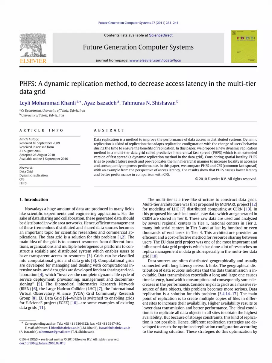
Fig. 1. A typical multi-tier data grid [29].

actions from the prior events. EPCM is originated from partitionedcontext modeling (PCM) and finite multi-order context (FMOC)modeling [27]. Grid access pattern modeling (GAPM) is proposedin [28] and has addressed the problem of data movement in thedata grid environment. This method extends the tier1 structureand PCM algorithm and uses them to predict future file needs inthe data grid and reduces job execution time by pre-fetching fileswhich are likely to be requested. PHFS like GAPM uses predictivemethod, but PHFS uses data mining techniques instead of the tierstructure and PCM algorithm to predict future needs. In PHFS, wecombine predictive method with the fast spread algorithm. Thismatter causes PHFS to become a suitable method in the multi-tierdata grid while GAPM is developed for a common data grid.

3. Predictive hierarchical fast spread

In this section, a new dynamic replication method in the multi-tier data grid called PHFSwill be presented. PHFS is an extension ofCFS. PHFS uses predictivemethods to predict future needs and pre-replicates them hierarchically in different nodes of different tiersin the multi-tier data grid on the path from the source node to theclient. As mentioned before, the multi-tier data grid is a tree-likestructure. Fig. 1 shows a typical multi-tier data grid [29].

In the multi-tier data grid, the nodes in upper layers have morestorage capacity and computational power than the lower levelnodes. Also, the bandwidth of the links between nodes in upperlevels is greater than the links in the lower level nodes. Therefore,the replication method in fast spread can replicate more items inupper level nodes and decrease the amount of replicated items onthe path to lower levels toward the client. The purpose of this kindof hierarchal replication is to optimize the utilization of resourcesfor replication and provide maximum locality with available re-sources.

In the first phase, PHFS collects the information of accesses fromall over the system and makes file access log files. Then, PHFSuses datamining techniques like association rules and clustering to

1 A tier is a data structure based on tree, but it is more efficient for storingpreviously seen access patterns and maintaining the count of each pattern.

mine the log files. This is done to discover useful knowledge such as(1) cluster of files that are accessed together with high probability,and (2) sequential access patterns that formmost frequently. It canbe said that these files have logical spatial locality. In other words,in the first phase, PHFS tries to find the relationship between filesfor future predictions.

We assume that we can find the relationship of all files by usingmining techniques on log files, without being concentrated on howit is done. The relationship between two files is shown by a numberin the 0–1 range, in which 1 implies that two files are completelyrelated, and 0 implies that they are not related at all. Having thesequantitative relations, themost related files to a specific file can beeasily determined. For this purpose, constant α (0 < α < 1) isconsidered as the criterion. Therefore, the files whose relationshipwith a specific file like A is greater than α are selected as the mostrelated files to A. Then, these files are arranged on the basis of thequantity of their relationship with A. This arrangement is called apredictive working set (PWS) for A. From spatial locality point ofview, the relation between files A and B indicates the probabilityof requesting file B after accessing A. Then, the members of PWS ofA are the most probable files that the requester of A may requestthem in the future.

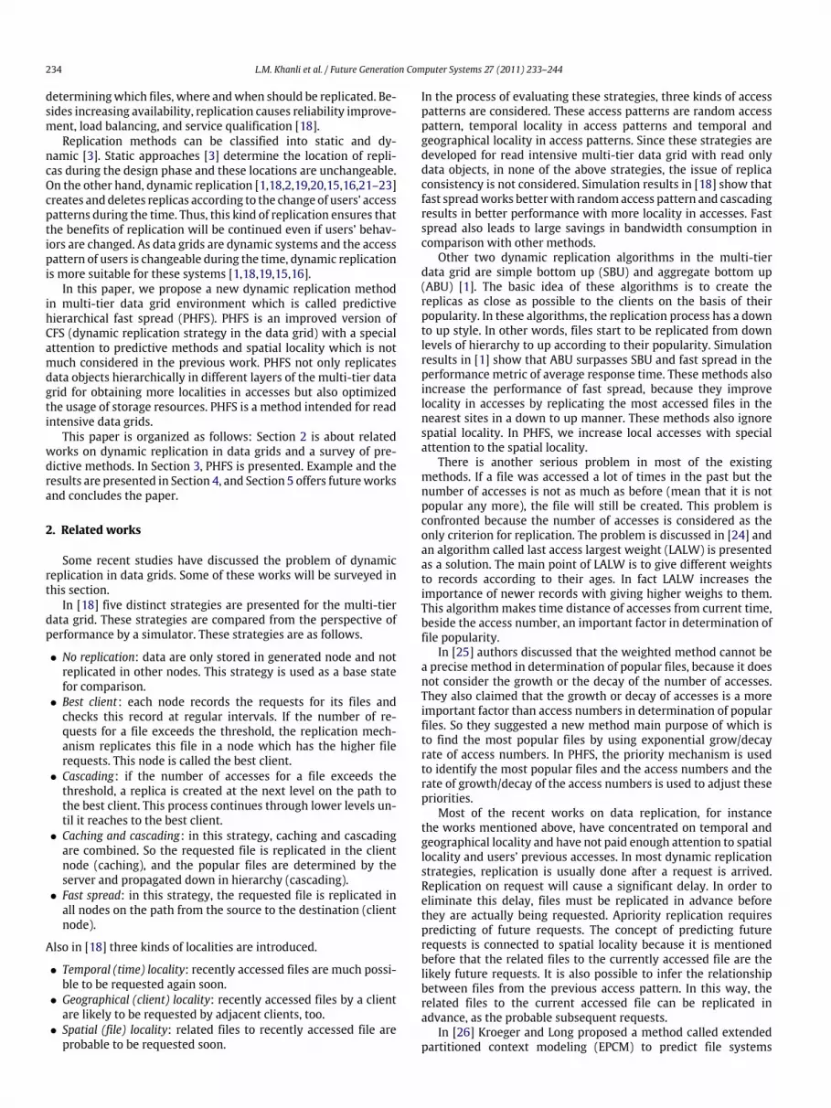
Despite the fact that the members of each PWS show spatiallocality, it is reasonable to suppose that each PWSwill exhibit someamount of geographical and temporal locality. In other words, it isexpected that the files in a PWS are accessed fromone region and inspecific period of time. Since the scientists tend to work in groupson projects, it can be assumed that some related files to the projectwill be requested by members from the region where the groupresides and during the project. Therefore when a client requests afile, PHFS finds the PWS of that file and replicates other elementsof PWS along with the requested file in a hierarchal manner fromthe root node to the client. Hierarchal manner means that PHFSreplicates all members of PWS in the first tier, and then replicate asubset of them which is related more than others to the requestedfile in second tier, and so on. For example suppose that B, C, D, E, F isthe PWS of A and client X requests file A. The way of replication byPHFS is illustrated in Fig. 2. As is shown in Fig. 2, in the second levelall members of PWS are replicatedwith A (in general the priority ofPWS and the available storage determine how many members ofeach PWS should be replicated, this issuewill be explained in detaillater) but in the third level only A, B, and C are replicated. Sincethe storage capacity of the third level is less than the second level,the number of replicated files should be reduced. According to theorder of members in PWS, it is expected that file B is requestedafter A with the highest probability, and file C is requested witha little lower probability than B and so on. Then in PHFS A, B,and C are replicated in the third level. And at the end, file A iscached in the client site. There is no constant rule to determinereplication configuration for all PWSs, because the state of eachPWS configuration depends on PWS priority. The priority of eachPWS originates from two parts. The first part is determined bythe system according to the priority of task (or user) which PWSbelongs to it. The second part comes from the number and the rateof accesses to PWS members during its existence in the system.High amount of access numbers and increasing access rate leads toan increase in the priority of a PWS or vice versa. By this definition,high priority means that the owner task of PWS is important orthe number of accesses to the members of PWS is high. The ideabehind this definition is that when the number of accesses to themembers of PWS is high or the rate of accesses is increasing, itis probable that PWS will be accessed more in the future. Dueto storage constraint in the nodes especially in lower levels, it isreasonable to replicate high priority PWSs more than low priorityones and also replicate most of their members in lower levels untilthey become closer to the client. Adjacency of the members of

236 L.M. Khanli et al. / Future Generation Computer Systems 27 (2011) 233–244

Fig. 2. An example of replication with PHFS. (1) Before replication. (2) Replication,after X request file A.

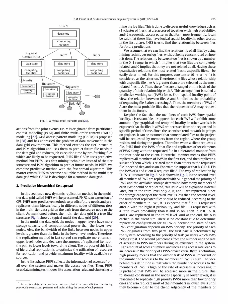
high priority PWS to the client causes more reduction in accesslatency and bandwidth consumption. Replication configuration ofdifferent PWS with different priorities is shown in Fig. 3. PWS1and PWS2 are two predictive working set with different priorities,and the priority of PWS1 is greater than PWS2. So the membersof PWS1 are replicated more than members of PWS2 and most ofthe members of PWS1 are replicated in the lower level. (PPWS1 >

PPWS2).

3.1. Architectural model of PHFS

As mentioned before, PHFS is a method that predicts subse-quent file requests on the basis of relationships between the files.It is also stated that the relationship between files can be inferredfrom the previous access patterns. Hence in PHFS, we need somemechanism for keeping previous accesses and analyzing them tofind the relationships. Therefore, PHFS has three phases: monitor-ing, analyzing, and replication.

• Monitoring: in the monitoring phase, a software agent in theroot node collects the file access information from all the clientsin the system and puts them in a log file.

• Analyzing: in the analyzing phase, the mining engine does datamining on log files and discovers useful information like therelationship between files.

• Replication: the replication phase is responsible for manage-ment of replicas and has the following two stages.◦ PWS construction stage: this stage of replication management

is activated when a file, which does not have any PWS in thesystem, is requested for the first time. In this situation repli-cation manager in the root node uses information providedby the mining engine and makes PWS for the requested file.Initial priority for constructed PWS is also assigned. This stageis only done in the root node. In fact this stage is the predic-tive stage of replication.

Fig. 3. Comparison of replication configuration of PWS with different priorities.

◦ Replica configuration adaptation stage: this stage is responsi-ble for adaption of replication configurationwith the existingsituation on the basis of the priority mechanism. This stage isdone with contribution of all replication managers which arepresent in all nodes.

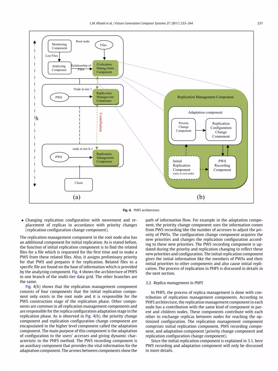
Monitoring and analyzing phase and also PWS construction stageof replication management are done centrally in the root node(the root can also use other nodes computational power in theanalyzing phase). This affair is shown in Fig. 4 (next page).

The second stage of replication management which is calledreplication configuration adaptation is done in a distributed waywith contribution of replica management components that existin all nodes except in the leaves (clients). The replication manage-ment component in each node has three main duties: (except inthe root node which has one additional function).

• Keeping the list of PWSs and their members in each node, andall other useful information (PWS recording component).

• Adjusting the priority of each PWS according to the accesshistory (priority change component).

L.M. Khanli et al. / Future Generation Computer Systems 27 (2011) 233–244 237

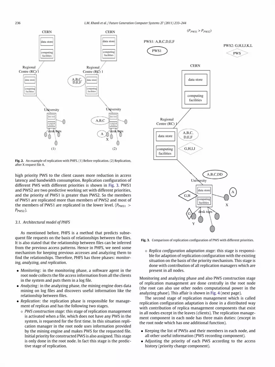
Fig. 4. PHFS architecture.

• Changing replication configuration with movement and re-placement of replicas in accordance with priority changes(replication configuration change component).

The replication management component in the root node also hasan additional component for initial replication. As is stated before,the function of initial replication component is to find the relatedfiles for a file which is requested for the first time and to make aPWS from these related files. Also, it assigns preliminary priorityfor that PWS and prepares it for replication. Related files to aspecific file are found on the base of information which is providedby the analyzing component. Fig. 4 shows the architecture of PHFSin one branch of the multi-tier data grid. The other branches arethe same.

Fig. 4(b) shows that the replication management componentconsists of four components that the initial replication compo-nent only exists in the root node and it is responsible for thePWS construction stage of the replication phase. Other compo-nents are common in all replicationmanagement components andare responsible for the replica configuration adaptation stage in thereplication phase. As is observed in Fig. 4(b), the priority changecomponent and replication configuration change component areencapsulated in the higher level component called the adaptationcomponent. Themain purpose of this component is the adaptationof configuration to the users’ accesses and giving dynamic char-acteristic to the PHFS method. The PWS recording component isan auxiliary component that provides the vital information for theadaptation component. The arrows between components show the

path of information flow. For example in the adaptation compo-nent, the priority change component uses the information comesfrom PWS recording like the number of accesses to adjust the pri-ority of PWSs. The configuration change component acquires thenew priorities and changes the replication configuration accord-ing to these new priorities. The PWS recording component is up-dated during the priority and replication changing to reflect thesenewpriorities and configuration. The initial replication componentgives the initial information like the members of PWSs and theirinitial priorities to other components and also cause initial repli-cation. The process of replication in PHFS is discussed in details inthe next section.

3.2. Replica management in PHFS

In PHFS, the process of replica management is done with con-tribution of replication management components. According toPHFS architecture, the replicationmanagement component in eachnode has a contribution with the same kind of component in par-ent and children nodes. These components contribute with eachother to exchange replicas between nodes for reaching the op-timized configuration. The replication management componentcomprises initial replication component, PWS recording compo-nent, and adaptation component (priority change component andreplication configuration change component).

Since the initial replication component is explained in 3.1, herePWS recording and adaptation component will only be discussedin more details.

238 L.M. Khanli et al. / Future Generation Computer Systems 27 (2011) 233–244

3.2.1. PWS recording componentThe function of the PWS recording component is to record the

useful information in each node. The information recorded in thePWS recording component is as follows:

• the lists of PWSs that exist on each node;• priorities of existed PWSs on each node;• members of existed PWS on that node;• also logs the accesses to each member of PWSs.

The above-mentioned information is used to change the priority ofPWSs in the priority change component and change the configura-tion of replication in the replication configuration component. Theinformation of PWS recording is updated when the priorities arechanged with priority change component and also when configu-ration of PWSs is changed with replication configuration changecomponent.

3.2.2. Adaptation componentIt consists of two components:

• priority change component and• replication configuration change component.

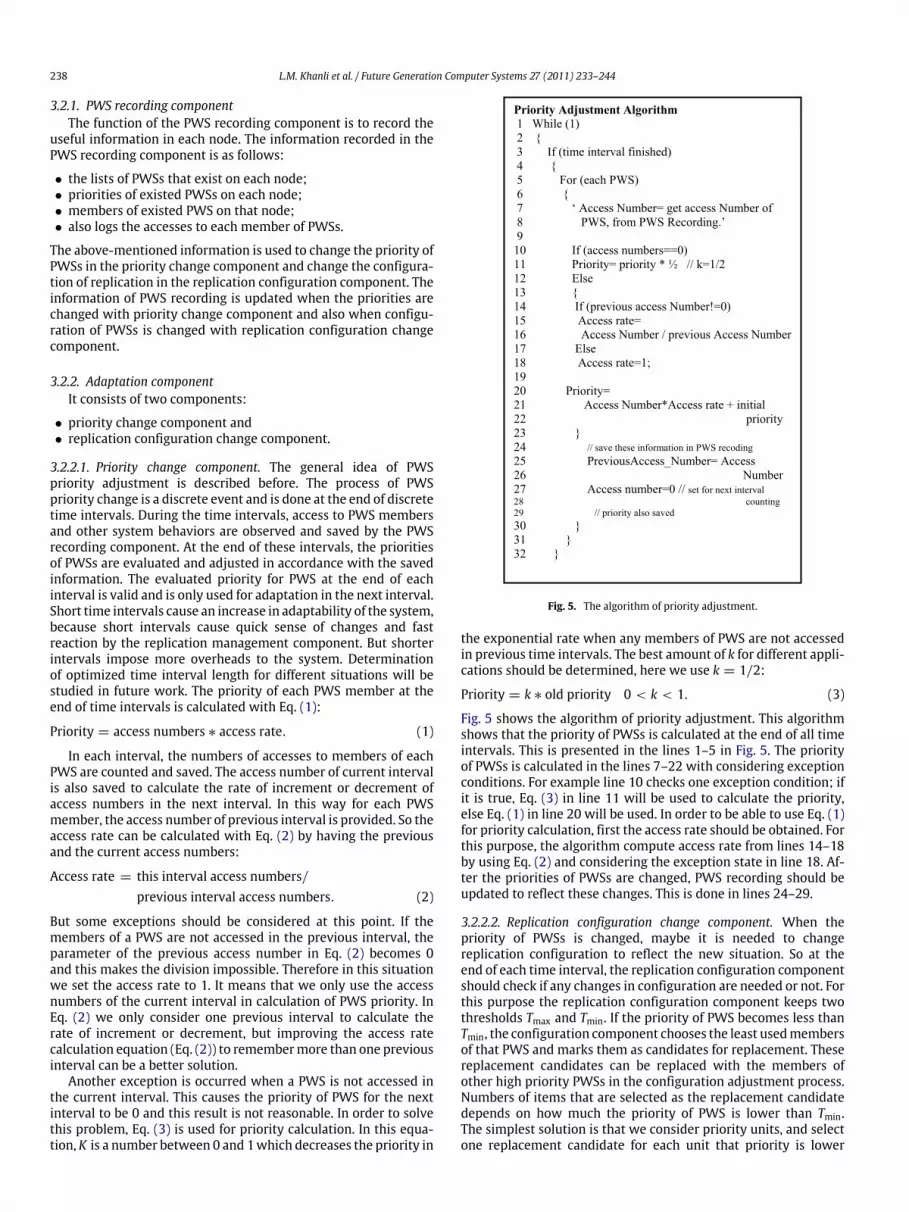
3.2.2.1. Priority change component. The general idea of PWSpriority adjustment is described before. The process of PWSpriority change is a discrete event and is done at the end of discretetime intervals. During the time intervals, access to PWS membersand other system behaviors are observed and saved by the PWSrecording component. At the end of these intervals, the prioritiesof PWSs are evaluated and adjusted in accordance with the savedinformation. The evaluated priority for PWS at the end of eachinterval is valid and is only used for adaptation in the next interval.Short time intervals cause an increase in adaptability of the system,because short intervals cause quick sense of changes and fastreaction by the replication management component. But shorterintervals impose more overheads to the system. Determinationof optimized time interval length for different situations will bestudied in future work. The priority of each PWS member at theend of time intervals is calculated with Eq. (1):

Priority = access numbers ∗ access rate. (1)

In each interval, the numbers of accesses to members of eachPWS are counted and saved. The access number of current intervalis also saved to calculate the rate of increment or decrement ofaccess numbers in the next interval. In this way for each PWSmember, the access number of previous interval is provided. So theaccess rate can be calculated with Eq. (2) by having the previousand the current access numbers:

Access rate = this interval access numbers/previous interval access numbers. (2)

But some exceptions should be considered at this point. If themembers of a PWS are not accessed in the previous interval, theparameter of the previous access number in Eq. (2) becomes 0and this makes the division impossible. Therefore in this situationwe set the access rate to 1. It means that we only use the accessnumbers of the current interval in calculation of PWS priority. InEq. (2) we only consider one previous interval to calculate therate of increment or decrement, but improving the access ratecalculation equation (Eq. (2)) to remembermore than one previousinterval can be a better solution.

Another exception is occurred when a PWS is not accessed inthe current interval. This causes the priority of PWS for the nextinterval to be 0 and this result is not reasonable. In order to solvethis problem, Eq. (3) is used for priority calculation. In this equa-tion, K is a number between 0 and 1which decreases the priority in

Fig. 5. The algorithm of priority adjustment.

the exponential rate when any members of PWS are not accessedin previous time intervals. The best amount of k for different appli-cations should be determined, here we use k = 1/2:

Priority = k ∗ old priority 0 < k < 1. (3)

Fig. 5 shows the algorithm of priority adjustment. This algorithmshows that the priority of PWSs is calculated at the end of all timeintervals. This is presented in the lines 1–5 in Fig. 5. The priorityof PWSs is calculated in the lines 7–22 with considering exceptionconditions. For example line 10 checks one exception condition; ifit is true, Eq. (3) in line 11 will be used to calculate the priority,else Eq. (1) in line 20 will be used. In order to be able to use Eq. (1)for priority calculation, first the access rate should be obtained. Forthis purpose, the algorithm compute access rate from lines 14–18by using Eq. (2) and considering the exception state in line 18. Af-ter the priorities of PWSs are changed, PWS recording should beupdated to reflect these changes. This is done in lines 24–29.

3.2.2.2. Replication configuration change component. When thepriority of PWSs is changed, maybe it is needed to changereplication configuration to reflect the new situation. So at theend of each time interval, the replication configuration componentshould check if any changes in configuration are needed or not. Forthis purpose the replication configuration component keeps twothresholds Tmax and Tmin. If the priority of PWS becomes less thanTmin, the configuration component chooses the least usedmembersof that PWS and marks them as candidates for replacement. Thesereplacement candidates can be replaced with the members ofother high priority PWSs in the configuration adjustment process.Numbers of items that are selected as the replacement candidatedepends on how much the priority of PWS is lower than Tmin.The simplest solution is that we consider priority units, and selectone replacement candidate for each unit that priority is lower

L.M. Khanli et al. / Future Generation Computer Systems 27 (2011) 233–244 239

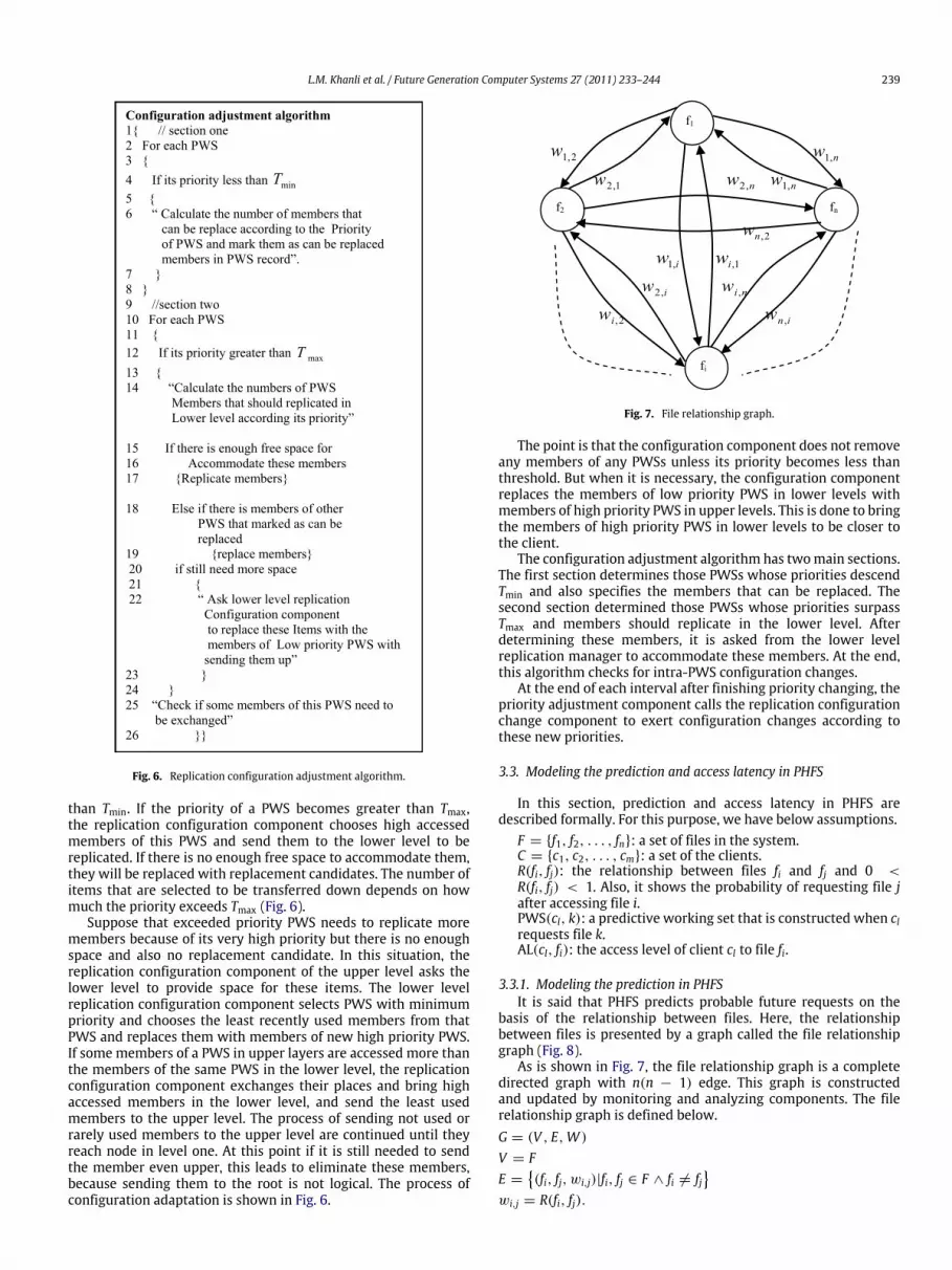
Fig. 6. Replication configuration adjustment algorithm.

than Tmin. If the priority of a PWS becomes greater than Tmax,the replication configuration component chooses high accessedmembers of this PWS and send them to the lower level to bereplicated. If there is no enough free space to accommodate them,they will be replaced with replacement candidates. The number ofitems that are selected to be transferred down depends on howmuch the priority exceeds Tmax (Fig. 6).

Suppose that exceeded priority PWS needs to replicate moremembers because of its very high priority but there is no enoughspace and also no replacement candidate. In this situation, thereplication configuration component of the upper level asks thelower level to provide space for these items. The lower levelreplication configuration component selects PWS with minimumpriority and chooses the least recently used members from thatPWS and replaces them with members of new high priority PWS.If some members of a PWS in upper layers are accessed more thanthe members of the same PWS in the lower level, the replicationconfiguration component exchanges their places and bring highaccessed members in the lower level, and send the least usedmembers to the upper level. The process of sending not used orrarely used members to the upper level are continued until theyreach node in level one. At this point if it is still needed to sendthe member even upper, this leads to eliminate these members,because sending them to the root is not logical. The process ofconfiguration adaptation is shown in Fig. 6.

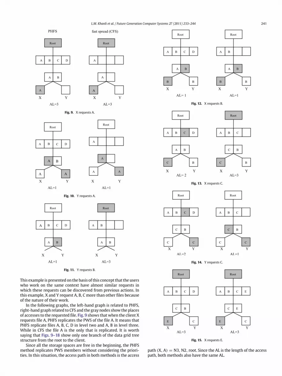
Fig. 7. File relationship graph.

The point is that the configuration component does not removeany members of any PWSs unless its priority becomes less thanthreshold. But when it is necessary, the configuration componentreplaces the members of low priority PWS in lower levels withmembers of high priority PWS in upper levels. This is done to bringthe members of high priority PWS in lower levels to be closer tothe client.

The configuration adjustment algorithm has twomain sections.The first section determines those PWSs whose priorities descendTmin and also specifies the members that can be replaced. Thesecond section determined those PWSs whose priorities surpassTmax and members should replicate in the lower level. Afterdetermining these members, it is asked from the lower levelreplication manager to accommodate these members. At the end,this algorithm checks for intra-PWS configuration changes.

At the end of each interval after finishing priority changing, thepriority adjustment component calls the replication configurationchange component to exert configuration changes according tothese new priorities.

3.3. Modeling the prediction and access latency in PHFS

In this section, prediction and access latency in PHFS aredescribed formally. For this purpose, we have below assumptions.

F = {f1, f2, . . . , fn}: a set of files in the system.C = {c1, c2, . . . , cm}: a set of the clients.R(fi, fj): the relationship between files fi and fj and 0 <R(fi, fj) < 1. Also, it shows the probability of requesting file jafter accessing file i.PWS(cl, k): a predictive working set that is constructed when clrequests file k.AL(cl, fi): the access level of client cl to file fi.

3.3.1. Modeling the prediction in PHFSIt is said that PHFS predicts probable future requests on the

basis of the relationship between files. Here, the relationshipbetween files is presented by a graph called the file relationshipgraph (Fig. 8).

As is shown in Fig. 7, the file relationship graph is a completedirected graph with n(n − 1) edge. This graph is constructedand updated by monitoring and analyzing components. The filerelationship graph is defined below.G = (V , E,W )

V = FE =

(fi, fj, wi,j)|fi, fj ∈ F ∧ fi = fj

wi,j = R(fi, fj).

240 L.M. Khanli et al. / Future Generation Computer Systems 27 (2011) 233–244

Fig. 8. Requested files with X and Y and the order of their requests.

On the basis of graph G, Rk(α) is defined as a set of files whoserelationship with file k is greater than α. The relationship of filesis presented with weights in relationship graph and α is theminimum amount of relationship that files should have until theyare considered as the most related files. α is a constant parameterthat is set before the running of the system. From spatial localitypoint of view, the weights (relationship between files) show theprobability of files being requested after each other. Hence, Rk(α)is a set of files where probability of being requested after file k isgreater than α. For example, if we set α = 0.5, Rk(α) is set of fileswhere probability of being requested after file k is greater than 0.5.

Then,

Rk(α) =fi|fi ∈ F ∧ (fk, fi, wk,i) ∈ E ∧ wk,i ≥ α

.

Rk(α) is constructed, when the client cl requests the file k from theroot node.

PWS(cl, k) as the PWS of the client cl for requesting the file k isa descended sort of Rk(α)

PWS(cl, k) = descended sort (Rk(α)).

Rk(α) is sorted because PHFS want to replicate the most relatedfiles to the file k in the lowest possible levels. Therefore, PHFSneeds to know which files are related to the file k more than theothers and which files are the most probable coming requests.Descended sorting of Rk(α) leads to sort the files according to theirrelationship with the file k and also according to the probability ofbeing requested after the file k. Thus, it can be deduced that theplaces of elements in PWS(cl, k) are important. In fact, PWS(cl, k)is a string of files. Here, [ ] are used to show strings. Then, we have

PWS(cl, k) = [k][fqi |fqi ∈ Rk(α) ∧ fqi ≥ fqi+1 ].

The index of q shows the position of fq in string. At the end, the filek is added to the beginning of the sorted files.

PWSs are only constructed in the root node. If a request for afile is not met in the middle nodes and reaches to the root node,the initial replication component makes a PWS for that requestand assigns a preliminary priority. Then, the files in PWS arereplicated along with the requested file as much as possible on itspath to the client who requests the file. While in the CFS method,just the requested file is replicated. In the process of replicatingPWS members, PHFS also tries to replicate the most related files(first members of PWS) in the lower nodes, because the mostrelated files are the most probable ones to be requested soon.Another important issue is the problem of prediction quality. Asis mentioned before, prediction is done on the basis of knowledgethat is achieved from log files. Therefore, because of poor log filesat the early stages of system’s operation, we should not expect ahigh-quality prediction.

3.3.2. Modeling the access latency in PHFSEach node in the system is identified by a unique ID and repre-

sented as a set of ordered pairs. The first component of each pairis a file which is placed on that node, and the second componenthas some information about the file. The information which can besaved for a file is the related PWS of the file, the numbers of ac-cesses in the current interval, the numbers of accesses in the pre-vious interval, and so on. All these metadata are considered as the

second component of the ordered pairs. This information is up-dated by the PWS recording component

NID = {(fi,metadata)|fi is in NIDnode}.

Since the multi-tier data grid is a tree-like structure, each clienthas only one path to the root and it is the path of its parents. Thismeans that the client can only ask his request from these parentsup to the root node. This request path of the client is defined as thepath of its parent:

request path(cl) = NID1,NID2, . . . , rootNIDs+1is the parent of NIDs

and NID1is the parent of client cl.

The request of the client goes through the request path until it ismet by one parent. Then, the access path of a client for a specificfile can be defined as a sub-path of the request path that requestgoes through to be met:

access path (cl, fi) = NID1,NID2, . . . ,NIDd

access path (cl, fi) ⊆ request path (cl)and fi is found in NIDd.

Therefore, when the file fi is accessed by the client cl, the accesslatency can be defined as follows:

AL(cl, fi) = | access path (cl, fi)| .

Themain aim of PHFS is to decrease the average AL of each individ-ual client. PHFS does this by predicting future demands and adap-tation mechanisms.

4. Comparison of fast spread and PHFS

In this section, PHFS and CFS are compared from access latencyperspective through an example. The assumptions for this exampleare as follows.

• The multi-tier data grid has four tiers like Fig. 1.• The node in level 2 has a storage space for four files and in level 3

has storage for two files. The client node can only accommodateone file.

• All files have the same size.• Latency for file transferring from one level to a lower level is

one unit of time.• Mining engine has discovered that A, B, C, D and E, F, G, H,

I are two sets of files that are accessed together with a highprobability.

• Tmax a threshold, for moving one item to a lower level, isconsidered two times.

• X and Y are two clients that work on a common project in onelab in the same region.

• Requested files with X and Y and their orders at a specific timeinterval is shown in Fig. 8.

• A comparison criterion is access latency (AL) in which loweraccess latency is the best condition. Since one unit of time isconsidered for latency between the layers, AL shows the leveldistance in access.

• Replacement strategy in both PHFS and CFS is the least recentlyused file.

• We do not consider any time delay for priority adjustment andconfiguration change. Priority adjustment and configurationchange happen immediately after any change in accesses.

• In this example, the ID of node in level 2 is N2 and the ID of nodein level 3 is N3.

L.M. Khanli et al. / Future Generation Computer Systems 27 (2011) 233–244 241

Fig. 9. X requests A.

Fig. 10. Y requests A.

Fig. 11. Y requests B.

This example is presented on the basis of this concept that the userswho work on the same context have almost similar requests inwhich these requests can be discovered from previous actions. Inthis example, X and Y request A, B, C more than other files becauseof the nature of their work.

In the following graphs, the left-hand graph is related to PHFS,right-hand graph related to CFS and the gray nodes show the placesof accesses to the requested file. Fig. 9 shows thatwhen the client Xrequests file A, PHFS replicates the PWS of the file A. It means thatPHFS replicate files A, B, C, D in level two and A, B in level three.While in CFS the file A is the only that is replicated. It is worthsaying that Figs. 9–18 show only one branch of the data grid treestructure from the root to the client.

Since all the storage spaces are free in the beginning, the PHFSmethod replicates PWS members without considering the priori-ties. In this situation, the access path in both methods is the access

Fig. 12. X requests B.

Fig. 13. X requests C.

Fig. 14. Y requests C.

Fig. 15. X requests E.

path (X,A) = N3,N2, root. Since the AL is the length of the accesspath, both methods also have the same AL.

242 L.M. Khanli et al. / Future Generation Computer Systems 27 (2011) 233–244

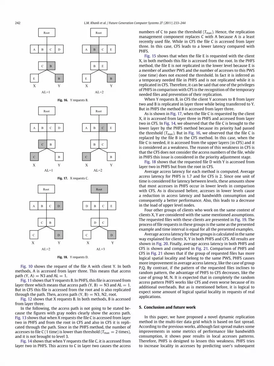
Fig. 16. Y requests B.

Fig. 17. X requests C.

Fig. 18. Y requests D.

Fig. 10 shows the request of the file A with client Y. In bothmethods, A is accessed from layer three. This means that accesspath (Y,A) = N3 and AL = 1.

Fig. 11 shows that Y requests B. In PHFS, this file is accessed fromlayer three which means that access path (Y, B) = N3 and AL = 1.But in CFS this file is accessed from the root and is also replicatedthrough the path. Then, access path (Y, B) = N3,N2, root.

Fig. 12 shows that X requests B. In both methods, B is accessedfrom layer three.

In the following, the access path is not going to be stated be-cause the figures with gray nodes clearly show the access path.Fig. 13 shows that when X requests the file C is accessed from layertwo in PHFS and from the root in CFS and also in CFS it is repli-cated through the path. Since in the PHFS method, the number ofaccesses to file C (1 time) is lower than threshold (Tmax = 2 times),and it is not brought to level 3.

Fig. 14 shows that when Y requests the file C, it is accessed fromlayer two in PHFS. This access to C in layer two causes the access

numbers of C to pass the threshold (Tmax). Hence, the replicationmanagement component replaces C with A because A is a leastrecently used file. While in CFS the file C is accessed from layerthree. In this case, CFS leads to a lower latency compared withPHFS.

Fig. 15 shows that when the file E is requested with the clientX, in both methods this file is accessed from the root. In the PHFSmethod, the file E is not replicated in the lower level because E isa member of another PWS and the number of accesses to this PWS(one time) does not exceed the threshold. In fact it is inferred asa temporary needed file in PHFS and is not replicated while it isreplicated in CFS. Therefore, it can be said that one of the privilegesof PHFS in comparisonwith CFS is the recognition of the temporaryneeded files and prevention of their replication.

When Y requests B, in CFS the client Y accesses to B from layertwo and B is replicated in layer three while being transferred to Y.But in PHFS the method B is accessed from layer three.

As is shown in Fig. 17, when the file C is requested by the clientX, it is accessed from layer three in PHFS and accessed from layertwo in CFS. In Fig. 14, we observed that the file C is brought to thelower layer by the PHFS method because its priority had passedthe threshold (Tmax). But in Fig. 16, we observed that the file C isreplaced by the file B in the CFS method. In this case, when thefile C is needed, it is accessed from the upper layers (in CFS) and itis considered as a weakness. The reason of this weakness in CFS isthat the CFS does not consider the access numbers of the file, whilein PHFS this issue is considered in the priority adjustment stage.

Fig. 18 shows that the requested file D with Y is accessed fromlayer two in PHFS but from the root in CFS.

Average access latency for each method is computed. Averageaccess latency for PHFS is 1.7 and for CFS is 2. Since one unit oftime is considered for latency between levels, these amounts showthat most accesses in PHFS occur in lower levels in comparisonwith CFS. As is discussed before, accesses in lower levels causea reduction in access latency and bandwidth consumption andconsequently a better performance. Also, this leads to a decreasein the load of upper level nodes.

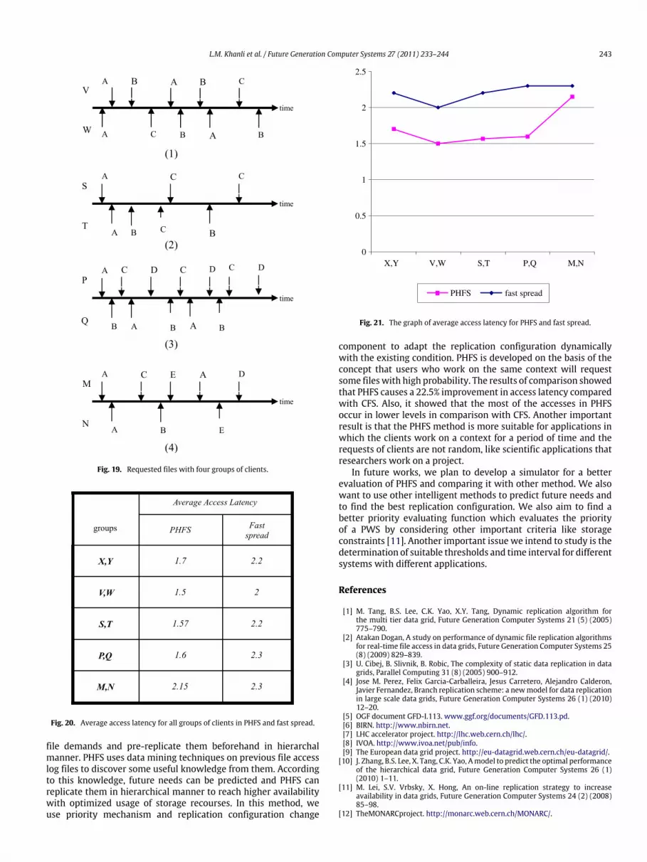
Four other groups of clients who work on the same context ofclients X, Y are considered with the samementioned assumptions.The requested files with these clients are presented in Fig. 19. Theprocess of file requests in these groups is the same as the presentedexample and time interval is equal for all the presented examples.

Average access latency for these groups is calculated in the sameway explained for clients X, Y in both PHFS and CFS. All results areshown in Fig. 20. Finally, average access latency in both PHFS andCFS is shown and compared in Fig. 21. Comparison of PHFS andCFS in Fig. 21 shows that if the group of requested files has morelogical spatial locality and belong to the same PWS, PHFS causesmore improvement in average access latency, like the case of groupP,Q. By contrast, if the pattern of the requested files inclines torandom pattern, the advantage of PHFS to CFS decreases, like thecase of group M, N. It is expected that in completely the randomaccess pattern PHFS works like CFS and even worse because of itsadditional overheads. But as is mentioned before, it is logical toexpect some amount of logical spatial locality in requests of realapplications.

5. Conclusion and future work

In this paper, we have proposed a novel dynamic replicationmethod in the multi-tier data grid which is based on fast spread.According to the previousworks, although fast spreadmakes someimprovements in some metrics of performance like bandwidthconsumption, it shows poor results in local accesses patterns.Therefore, PHFS is designed to lessen this weakness. PHFS triesto increase locality in accesses by predicting user’s subsequent

L.M. Khanli et al. / Future Generation Computer Systems 27 (2011) 233–244 243

Fig. 19. Requested files with four groups of clients.

Fig. 20. Average access latency for all groups of clients in PHFS and fast spread.

file demands and pre-replicate them beforehand in hierarchalmanner. PHFS uses data mining techniques on previous file accesslog files to discover some useful knowledge from them. Accordingto this knowledge, future needs can be predicted and PHFS canreplicate them in hierarchical manner to reach higher availabilitywith optimized usage of storage recourses. In this method, weuse priority mechanism and replication configuration change

Fig. 21. The graph of average access latency for PHFS and fast spread.

component to adapt the replication configuration dynamicallywith the existing condition. PHFS is developed on the basis of theconcept that users who work on the same context will requestsome fileswith high probability. The results of comparison showedthat PHFS causes a 22.5% improvement in access latency comparedwith CFS. Also, it showed that the most of the accesses in PHFSoccur in lower levels in comparison with CFS. Another importantresult is that the PHFS method is more suitable for applications inwhich the clients work on a context for a period of time and therequests of clients are not random, like scientific applications thatresearchers work on a project.

In future works, we plan to develop a simulator for a betterevaluation of PHFS and comparing it with other method. We alsowant to use other intelligent methods to predict future needs andto find the best replication configuration. We also aim to find abetter priority evaluating function which evaluates the priorityof a PWS by considering other important criteria like storageconstraints [11]. Another important issue we intend to study is thedetermination of suitable thresholds and time interval for differentsystems with different applications.

References

[1] M. Tang, B.S. Lee, C.K. Yao, X.Y. Tang, Dynamic replication algorithm forthe multi tier data grid, Future Generation Computer Systems 21 (5) (2005)775–790.

[2] Atakan Dogan, A study on performance of dynamic file replication algorithmsfor real-time file access in data grids, Future Generation Computer Systems 25(8) (2009) 829–839.

[3] U. Cibej, B. Slivnik, B. Robic, The complexity of static data replication in datagrids, Parallel Computing 31 (8) (2005) 900–912.

[4] Jose M. Perez, Felix Garcia-Carballeira, Jesus Carretero, Alejandro Calderon,Javier Fernandez, Branch replication scheme: a newmodel for data replicationin large scale data grids, Future Generation Computer Systems 26 (1) (2010)12–20.

[5] OGF document GFD-I.113. www.ggf.org/documents/GFD.113.pd.[6] BIRN. http://www.nbirn.net.[7] LHC accelerator project. http://lhc.web.cern.ch/lhc/.[8] IVOA. http://www.ivoa.net/pub/info.[9] The European data grid project. http://eu-datagrid.web.cern.ch/eu-datagrid/.

[10] J. Zhang, B.S. Lee, X. Tang, C.K. Yao, Amodel to predict the optimal performanceof the hierarchical data grid, Future Generation Computer Systems 26 (1)(2010) 1–11.

[11] M. Lei, S.V. Vrbsky, X. Hong, An on-line replication strategy to increaseavailability in data grids, Future Generation Computer Systems 24 (2) (2008)85–98.

[12] TheMONARCproject. http://monarc.web.cern.ch/MONARC/.

244 L.M. Khanli et al. / Future Generation Computer Systems 27 (2011) 233–244

[13] CERN. http://public.web.cern.ch/Public/Content/Chapters/AboutCERN/AboutCERN-en.html.

[14] M.M. Deris, J.H. Abawajy, A. Mamat, An efficient replicated data accessapproach for large-scale distributed systems, Future Generation ComputerSystems 24 (1) (2008) 1–9.

[15] K. Ranganathan, I. Foster, Simulation studies of computation and datascheduling algorithms for data grids, Journal of Grid Computing 1 (1) (2003)63–74.

[16] M. Tang, B.S. Lee, X. Tang, C.K. Yeo, The impact of data replication on jobscheduling performance in thedata grid, FutureGenerationComputer Systems22 (3) (2006) 254–268.

[17] P. Kunszt, E. Laure, H. Stockinger, K. Stockinger, File-based replica manage-ment, Future Generation Computer Systems 22 (1) (2005) 115–123.

[18] K. Ranganathan, I. Foster, Identifying dynamic replication strategies for highperformance data grids, in: Proceedings of the Second InternationalWorkshopon Grid Computing, Denver, CO, November 2001, pp. 75–86.

[19] D.G. Camaron, A.P. Millar, C. Nicholson, R.C. Schiaffino, F. Zini, K. Stockinger,Analysis of scheduling and replica optimisation strategies for data grids usingoptorsim, Journal of Grid Computing 2 (1) (2004) 57–69.

[20] H. Lamehamedi, Z. Shentu, B. Szymanski, E. Deelman, Simulation of dynamicdata replication strategies in data grids, in: Proceeding of 12th HeterogeneousComputing Workshop, Nice, France, April 2003.

[21] H. Lamehamedi, B.K. Szymanski, Decentralized data management frameworkfor data grids, Future Generation Computer Systems 23 (1) (2007) 109–115.

[22] X. Dong, J. Li, Z. Wu, D. Zhang, J. Xu, On dynamic replication strategies in dataservice grids, in: Proceeding of 11th IEEE Symposium on Object Oriented Real-Time Distributed Computing, ISORC, 2008.

[23] S.M. Park, J.H. Kim, Y.B. Ko, W.S. Yoon, Dynamic data grid replication strategybased on internet hierarchy, in: Proceeding of Second InternationalWorkshopon Grid and Cooperative Computing, GCC’2003.

[24] R.S. Chang, H.P. Chang, A dynamic data replication strategy using access-weights in data grids, The Journal of Supercomputing 45 (3) (2008) 277–295.

[25] M.K. Madi, S. Hassan, Dynamic replication algorithm in data grid: survey, in:Proceeding of International Conference on Network Applications, Protocolsand Services, 22 November 2008.

[26] T.M. Kroeger, D.D.E. Long, Design and implementation of a predictive fileprefetching algorithm, in: Proceedings of the 2001 USENIX Annual TechnicalConference, Boston, Massachusetts, USA, June 25–30.

[27] T.M. Kroeger, D.D.E. Long, Predicting file system actions from prior events,in: Proceedings of the 1996 Annual Conference on USENIX Annual TechnicalConference, San Diego, CA, 1996.

[28] R.Shiung Chang, Ning Yuan Huang, Jih Sheng Chang, A predictive algorithmfor replication optimization in data grid, in: Proceeding of ICS 2006, Taiyuan,Taiwan, 2006, pp. 199–204.

[29] W. Hoschek, J.J. Martinez, A. Samar, H. Stockinger, K. Stockinger, Datamanagement in an international data grid project, in: Proceeding of the IEEE,ACM InternationalWorkshop on Grid Computing, Grid’2000, Bangalore, India,17–20 December 2000.

Leyli Mohammad Khanli received her B.S. (1995) fromShahid Beheshti University Tehran, Iran, M.S. (2000)from IUST (Iran University of Science and Technology)University and a Ph.D. degree (2007) from IUST (IranUniversity of Science and Technology)University. All are incomputer engineering. She is currently assistant professorin the Department of Computer Science at University ofTabriz. Her research interests include grid computing andQuality of Service management.

Ayaz Isazadeh is an associate professor in the Departmentof Computer Science at University of Tabriz. He receiveda B.Sc. degree in Mathematics from University of Tabrizin 1971, an M.S.Eng. degree in Electrical Engineering andComputer Science from Princeton University in 1978, anda Ph.D. degree in Computing and Information Science fromQueen’s University. The areas of his Research and TeachingInterests include, Automata Theory and Formal Languages,Software Engineering, Management Information Systems(MIS), Information and Communication Technology (ICT),Data Structures and Algorithms.

Tahmures N. Shishevan Since 2008, he is aMSA candidatein the Department of Computer science at University ofTabriz. His research interests include grid computing.